Entitled to Work:

Urban Property Rights and Labor Supply in Peru

Erica Field†

Harvard University

This version: July 2003

Abstract: Over the past decade, the Peruvian government issued property titles to over 1.2 million urban households, the largest government titling program targeted to urban squatters in the developing world. This paper examines the labor market effects of increases in tenure security resulting from the program. In particular, I study the direct impact of securing a property title on hours of work, location of entrepreneurial activity and child labor force participation. To isolate the causal role of ownership security I make use of differences across regions induced by the timing of the program and differences across target populations in the level of pre-program tenure security. My estimates suggest that titling results in a substantial increase in labor hours, a shift in labor supply away from work at home to work in the outside market and substitution of adult for child labor. For the average squatter family, granting of a property title is associated with a 17% increase in total household work hours, a 47% decrease in the probability of working inside the home, and a 28% reduction in the probability of child labor. Keywords: Property rights, land titling, development policy, urban economics, time allocation and labor supply, employment determination and creation JEL Categories: P14, Q15, J0, J22, R0, O18, O54

†ACKNOWLEDGEMENTS: I am indebted to Hank Farber and Anne Case for generous support throughout this project and to Daniel Andaluz in the COFOPRI office for providing the survey data. I also thank Attila Ambrus, David Autor, Melissa Clark, Javier Escobal, Eszter Hargittai, Chang-Tai Hsieh, Jeff Kling, Lewis Kornhauser, David Linsenmeier, Kristin Mammem, Alex Mas, Ted Miguel, Ceci Rouse, Máximo Torero, Diane Whitmore, IRS labor lunch, RPDS workshop, GRADE seminar and NYU colloquium participants for numerous useful comments.

1

1 Introduction

Strengthening economic institutions is widely argued to foster investment in physical and

human capital, bolster growth performance, reduce macroeconomic volatility and encourage an

equitable and efficient distribution of economic opportunity (Acemoglu et al., 2002; North,

1981). As one of the basic roles of institutions and fundamental to all economic transactions,

codifying and protecting property rights is seen in many academic discussions as requisite for

economic development and poverty reduction. 1 Among policy-makers as well, property titling is

increasingly considered one of the most effective forms of government intervention for targeting

the poor and encouraging economic growth (Baharoglu, 2002; Binswanger et al, 1995). Despite

the consensus on the importance of institutional factors for economic performance, there is a

shortage of reliable estimates of the influence of property reforms on a range of market

outcomes. This paper studies the impact of property rights on labor markets in developing

countries by analyzing household labor supply responses to exogenous changes in formal

ownership status. In particular, I assess the value to a squatter household of increases in tenure

security associated with obtaining a property title in terms of hours of labor supply gained and

improved efficiency of labor allocation between home and market work and between child and

adult labor.

An obstacle to measuring the influence of tenure security is the potential endogeneity of

ownership rights.2 I circumvent the problem by using data from a dramatic natural experiment in

Peru, in which a nationwide program issued formal property titles over a five-year period to

more than 1.2 million urban households. This approach in large measure breaks the link between

1 See, generally, Demsetz (1967), Alchian and Demsetz (1973) and Shleifer et al. (2001). 2 Direct evidence of this is provided by Miceli et al. (2001), who analyze the extent of endogeneity of formal agricultural property rights in Kenya.

2

tenure security and income and helps isolate the causal effect of property titling on market

outcomes. Although no panel data are available on program participants, extensive cross-

sectional data were collected on past and future title recipients mid-way through the program,

generating a natural set of comparison groups composed of treated and yet-to-be-treated

households. The Peruvian titling program constitutes the first large-scale urban property rights

reform that has occurred in the developing world, and its impact has implications for many

developing countries in which urban squatting is a widespread phenomenon.

An important contribution of this paper is the specific focus on non-agricultural

households and the value to urban residents of increased ownership security. In developing

countries, large proportions of urban and rural residents alike lack tenure security. Yet,

presumably because of historic interests in agricultural investment and related politics of land

reform, the majority of both academic and policy attention to property rights reform has centered

on rural households’ tenure insecurity. Nevertheless, in most of the developing world, the

population – and particularly the impoverished population – is increasingly urban. 3 Though

advocates of urban property reform cite many of the same benefits to land titling for non-

agricultural as for farm households, the relationship between tenure security and economic

efficiency is likely to be distinct in the urban setting. In particular, as will be addressed in this

paper, there is cause to believe that urban employment levels are particularly sensitive to the

degree of residential formalization.

In this manner, the paper also contributes to the literature by examining a unique aspect

of the welfare gains to property titling: the effect of improvements in tenure security on labor

supply and labor allocation decisions within the household. The fundamental consequence of

3 In Latin America and the Caribbean, for instance, the population shifted between 1950 and 2000 from 41% to 75% urban (United Nations, World Urbanization Prospects: The 1999 Revision, 2000).

3

successful residential formalization is a reduction in the household’s likelihood of forced

eviction by the government or expropriation by other residents. As long as untitled households

expend their own human resources in an effort to solidify informal claims to land, the acquisition

of a property title has direct value in terms of freeing up hours of work previously devoted to

maintaining tenure security through informal means and securing formal rights. As the following

quote illustrates, there is ample anecdotal evidence that urban squatters are commonly

constrained by the need to keep a family member at or close to home to protect against

residential property invasion:

“‘I go to work, and my mother looks after the house,’ says Alejandrina Matos Franco, who sells cassettes on the street in Lima and who worries that people could seize her house when she is away.” (Conger, 1999) In addition, the legal process of acquiring formal property titles traditionally involved

substantial monetary and time costs.4 Both factors clearly raise untitled households’ labor needs

for production of home security and in turn the opportunity cost of employment outside the

home. As a result, untitled households make constrained decisions in allocations of leisure, home

production, and the amount of child relative to adult labor.

To study these relationships, I implement a quasi-experimental empirical strategy using

cross-section micro-data from a survey of past and future beneficiaries of the Peruvian titling

program. Two sources of variation in program influence are used to isolate the effect of titling:

neighborhood program timing and program impact based on prior household ownership status. In

particular, staggered regional program timing enables a comparison of households in

neighborhoods already reached by the program with households in neighborhoods not yet

reached. Meanwhile, variation in pre-program tenure security allows residents not subject to

4 According to one report, “In Peru, the process of getting a deed from the bureaucracy involved 207 steps divided among 48 government offices, took an average of 48 months to complete, and was too expensive for small property owners.” (Economist, 1995)

4

changes in security to serve as a quasi-control group for residents who experience relatively large

changes as a result of the program.

The fact that the program targeted nearly all untitled households regardless of household

demand for formal property rights also enables a broader exploration of heterogeneity in

response to the program. Heterogeneity in the demand for property titles has been shown to

depend heavily on factors which contribute to the cost of maintaining informal rights.5 For this

purpose, both residential tenure – a proxy for informal tenure security – and household size are

used as indicators of the relative value of a property title for a given household. Given that

overall “de facto” property rights are observed to increase with residential tenure, the value of a

property title and therefore the program impact should be lower for households with longer

residential tenure (De Soto, 1986). Likewise, since (for a given property size) households with

more adults have greater capacity to provide home security, the tenure security value of a formal

title should be lower for larger families.

Several interesting findings emerge. My estimates of early program impact suggest that

households with no legal claim to property spend an average of 16.2 hours per week maintaining

informal tenure security, reflecting a 17% reduction in total household work hours for the

average squatter family. Also, households are 47% more likely to work inside of their home.

Thus, the net effect of property titling is a combination of an increase in total labor force hours

and a reallocation of work hours from inside the home to the outside labor market. My estimates

further support the predictions that informal property rights and household size influence the

home security demands facing an untitled household. For all labor supply measures, the effect of

obtaining a property title is decreasing in residential tenure and in the number of working-age

household members. Finally, for households with children, urban land titling is associated with a 5 In fact, heterogeneity in the demand for property titles is modeled explicitly in Miceli et al. (2001).

5

28% lower probability of child labor force participation. The results are particularly convincing

in light of a number of possible downward biases.

The next section of the paper reviews the theoretical and empirical literature on land

rights in developing countries. The third section describes the titling program in greater detail.

The fourth section presents a model of household labor supply in which, under very general

conditions, total labor supplied to the outside market unambiguously rises with an increase in

formal property rights, and both labor hours in home production and child labor unambiguously

fall. The fifth section describes the empirical model and discusses the identification strategy for

program effect. The sixth section presents results and robustness checks. The seventh section

discusses long-run predictions and the eighth section concludes.

2 Related Literature

There exists a wide body of literature demonstrating the positive influence of property

institutions on market outcomes. Several macroeconomic analyses have shown a relationship

between economic development and cross-country variation in institutional strength, which

encompasses property institutions (Knack et al., 1995; Mauro,1995; Hall et al.,1999;

Rodrik,1999). In the microeconomic literature, the link between property rights and welfare

enhancement has generally been confined to three channels established in a seminal paper by

Besley (1995) that explores the benefits of ownership rights for agricultural households. These

are: increased tenure security and greater investment incentives, lower transactions costs and

gains from trade in land, and greater collateral value of land and improved credit access. The

relationship between land rights and labor markets has been mentioned only in the context of

6

residential mobility and labor market adjustment, a corollary implication of higher transaction

costs in real estate (Yao, 1996; World Development Report, 2000; Moene, 1992).

Empirical estimates of the value of property titles in agricultural settings corroborate

these predictions. Studies such as Alston et al. (1996), Lopez (1997) and Carter and Olinto

(1997) link land titles with improved credit access, while many authors including Feder (1998),

Besley (1995), Banerjee et al. (2002) and Alston et al. (1996) provide evidence that lack of

property title indeed affects agricultural investment demand.6 In urban settings, the value of

property titles has been measured far less often and empirical work has focused primarily on real

estate prices. A major contribution is a paper by Jimenez (1984), involving an equilibrium model

of urban squatting in which it is shown that the difference in unit housing prices between the

non-squatting (formal) sector of a city and its squatting (informal) sector reflects the premium

associated with tenure security. The accompanying empirical analysis of real estate markets in

the Philippines finds equilibrium price differentials between formal and informal sector unit

dwelling prices in the range of 58%, and greater for lower income groups and larger households.

Consistent with the agricultural investment literature, Hoy and Jimenez (1996) find that land

titles are also associated with greater local public goods provision in squatter communities in

Indonesia.

A separate line of research on property institutions relates to the role of informal or “de

facto” property rights. A number of authors such as Carter (1994, 1996) and Galal and Razzaz

(2001) note that, in many settings, informal institutions arise to compensate for the absence of

formal property protection. Thus, legal enforcement constraints are binding only insofar as they

correspond to real tenure insecurity. Lanjouw and Levy (2002) find that levels of informal 6 Other work, such as Migot-Adholla et al. (1998) and Kimuyu (1994) detect little impact of land titling on investment. The mixed results are commonly attributed to the difficulty of addressing the endogeneity of title status.

7

property rights vary greatly in urban communities in Ecuador, and de facto tenure security varies

systematically with observable household characteristics such as sex of household head and

length of residence. In addition, their paper demonstrates that the value of a formal title can be

overestimated by real estate price differentials when non-transferable informal rights are ignored.

In my paper, the concept of informal rights is further extended to comprise not only exogenous

household characteristics, but also home security investment choices.

3 Project Background

This paper examines the effects of the Peruvian government’s recent series of legal,

administrative and regulatory reforms aimed at promoting a formal property market in urban

squatter settlements. Peru's informal urban settlements grew out of the massive urban-rural

migration that occurred over the last half-century as a result of the collapse of the rural economy

(due in part to a failed land reform program) and the growth of terrorism. The existence of

extensive barren land owned by the state on the perimeters of major cities along with an implicit

housing policy during the 1980s that allowed squatter settlements on unused government lands

led to an extended era of urban migration, often in the form of organized invasions by squatters

from the same area of emigration (Olórtegui, 2001).7 It is estimated that in 1997, a quarter of

Peru’s urban population lived in marginal squatter settlements in peri-urban areas and many

more untitled residents occupied inner-city neighborhoods (World Bank, 1997b).8

Prior to the reforms, obtaining a property title for a Peruvian household was nearly

impossible due to heavy bureaucratic procedures and prohibitive fees. As described in the initial

7 Invasion of privately-owned property was allowed by law if the land had been unused for a period of four years. The law has since changed (in 1990) so that invasions of private property are not allowed under any circumstances. 8 See Appendix A for a country map of the untitled population and properties targeted for formalization.

8

project report: “Peru’s traditional system of titling and registration is complex, inefficient,

expensive – prohibitively so for poor people – and prone to rent-seeking. Fourteen different

agencies are involved in the generation of each title, the courts have rarely been able to validate

these titles as the law requires…” (World Bank, 1998a).9 Due to acute housing shortages and

lack of legal transparency, tenants struggled not only with the government but also among

themselves to secure residential properties. The common failure of the government to defend or

even recognize informal tenure rights in individual disputes gave rise to rent-seeking behavior in

the form of invasions of untitled land (Olórtegui, 2001).

In 1991, a Peruvian non-governmental organization embarked on an innovative property

titling project in the capital city of Lima whose goal was “the rapid conversion of informal

property into securely delineated land holdings by the issuing and registering of property titles”

(World Bank, 1998b). Between 1992 and 1995, roughly 200,000 titles were issued at an

extremely low cost, convincing the government and a growing international audience of the

potential for efficiency gains from urban property formalization (World Bank, 1998a). In 1996,

under the auspices of the public agency COFOPRI (Committee for the Formalization of Private

Property) and Decree 424: Law for the Formalization of Informal Properties, the Peruvian

government established a national property registry based on the early model to formalize the

remaining properties in Lima and extend the program to seven other cities.10

Just as in the pilot project, implementation of the national program involved area-wide

titling by neighborhood, which was “presumed to foster, through community participation and

9 In his groundbreaking study of the underground economy, economist Hernando de Soto documented the same phenomenon: “In ‘The Other Path’, de Soto and aids concluded that … to get title to a house in an informal settlement whose permanence the government had already acknowledged took 728 steps from one agency alone, and ten other agencies also required approval” (Rosenberg, 2000). 10 According to the World Bank Project Appraisal Document (1998), target cities were chosen according to a formula based on city size, density of informal settlements, and distance from commercial centers, measures indicating the likely ease and cost of formalization and the expected poverty impact.

9

education, a demand for formalization, reduce the unit cost of formalization, and rapidly generate

a minimum critical mass of beneficiaries” (World Bank, 1997c). While the old process of

acquiring a property title was prohibitively slow and expensive, the new process was free and

extremely rapid. Once a local property registration system was set up, local program officials

were trained, and the city’s target areas were properly identified and mapped, several project

teams simultaneously entered neighborhoods starting from different points in the city. 11 To be

eligible for program participation, title claimants were required to verify residency predating

1995, and had to live on eligible public properties.12 As a result of the reforms, by December

2001 nearly 1.2 million of the country’s previously unregistered residents became nationally

registered property owners, affecting approximately 6.3 million of the roughly 10 million

untitled residents living in the range from just above to below the poverty line.13

In the realm of literature on the economic benefits of tenure security, the Peruvian

experience provides a unique research opportunity for many reasons. Briefly, the national

formalization plan constitutes a one-of-a-kind natural experiment worldwide in terms of

providing nearly cost-free improvements in ownership security on such a large scale.

Furthermore, unlike many large-scale government programs, the titling efforts took place at an 11 In campaigns of two months each, project teams entered 50 to 70 neighborhoods encompassing roughly 30,000 to 35,000 plots. Within a neighborhood, teams spent five to seven weeks establishing residential claims and delineating properties before conferring state-registered property titles onto all eligible residents. The registration process for these titles took an additional period of one to six months. 12 Ineligible properties included archeological sites and flood planes, among other exceptions – see page 22 for a description. In the COFOPRI data, 9.42% of sampled households are ineligible according to reported length of residence, and an additional 10% remain untitled after several years of program operation. 13 Though the grant period is not yet over until December 2002, thus far, 1.64 million lots have already been formalized and 1.21 million titles granted, the vast majority of which took place between 1998 and 2000. While no residents who previously possessed registered municipal titles are included in this figure, it is uncertain what fraction of this number had locally registered sales documents before the national reforms as these households were included in the government’s definition of “untitled”, though in reality the program simply transferred such titles to the national registry. In my paper, the term squatter refers only to households with no sales or judicial titles prior to the reforms, which is estimated to be 37% of the target population.

10

extremely rapid pace, which facilitates program evaluation by eliminating much of the need to

consider time trends that could obscure the independent effects of program participation. At the

same time, in the absence of panel data on participating households, the fact that program timing

was staggered proves to be an asset for evaluation purposes. A survey of 2750 urban households

was conducted in March 2000 midway through program implementation. Because the sample

was drawn from the universe of all target populations for eventual program intervention, the data

contain a number of households in neighborhoods in which the program has not yet entered.

4 Conceptual Framework

4.1 Total Household Labor Supply

This section presents a household production model that formalizes the intuition that, in a

setting of incomplete property rights, the standard labor-leisure choice will be influenced by

household demand for security of property. There are three principal mechanisms by which it is

assumed that tenure insecurity removes individuals from the labor force. First, individuals in

untitled households are constrained by the need to provide informal policing, both to deter

prospective invaders from targeting individual properties and to participate in community

enforcement efforts to protect the neighborhood boundaries.14 If prospective squatters seek out

abandoned land, signaling that the property is occupied may deter conflicts over land or property

boundaries. Second, reducing the probability of government eviction at the community level may

require a critical mass of individuals squatting on neighborhood land, particularly in early stages

of community formation. As a result, social norms may evolve at the community level such that 14 In a related sense, it is reasonable to assume that untitled households feel a greater threat of robbery given that it is more costly for them to rely on local law enforcement in addition to the fact that households that do not have legal rights to a residence may have less legal claim to property inside the home.

11

households that do not spend time squatting on neighborhood land, which is good for the entire

neighborhood, are punished by other community members. Finally, households may attempt to

increase tenure security through formal channels by going through administrative steps to

acquire land rights.

In addition, greater tenure security may encourage household members to work on

account of an increase in the value of consumption of immobile assets such as housing

infrastructure. As discussed at the end of the section, the entire set of predictions from the

following theoretical model allows me to test empirically whether the labor supply response to

improvements in tenure security is driven in part by a change in the security value of leisure.

I capture the influence of these incentives on labor supply in a simple variation of the

basic agricultural household model The main innovation is the incorporation of a tenure security

function, )(⋅s , into the utility function, such that both leisure and home production enter

household utility through two separate channels: through their respective consumption and

production values and through their effect on home security. 15 Furthermore, the security value of

time at home is sensibly modeled as a household public good, such that individual utility

depends on the leisure and home production hours of all other members via )(⋅s . In this

framework, utility, given a set of household characteristics ψ and resource endowment E, is an

increasing function of per capita leisure, consumption, and home security, and home security is

determined by the following three parameters: total hours of household time at home (time spent

by family members “protecting” property), an exogenous parameter, θ , which reflects the

15 As opposed to models of joint production in the vein of Gronau (1977), I assume incomplete substitution between market goods and home security due to the absence of an outside market for home security protection.

12

household’s level of formal property rights, and a summary measure, τ , which reflects the

degree of informal or “de facto” rights the household has acquired.

For tractability, I make the following set of assumptions. First, the household is assumed

to maximize per capita leisure and not the leisure of individual members. Given that this model

is concerned with the effect of θ on total household labor, ignoring the second stage of the

household decision problem in which leisure is allocated across individual members is

inconsequential to the central results. Second, there is no outside labor market for the provision

of home security. Assuming a missing labor market for property protection is easily justified by

an incomplete contracts argument (there is risk involved in employing non-members to guard

property), although a more complicated model would have this market depend on θ .16

Furthermore, while the model does not explicitly include hired security, there is room to

incorporate the existence of a black market for property protection into τ . Fourth, as opposed to

models of joint production such as Graham and Green (1984), in this model leisure and home

production hours are assumed to be perfect substitutes for the hours an individual spends on

property protection. 17 Finally, this is a unitary household model, and it is assumed that all

household members face a common wage, w.

Let N be the number of household members, and li be leisure, xi consumption, hfi labor

hours in home production, and hoi outside labor hours of household member i, and

∑=

=N

iilL

1

, ∑=

=N

ifif hH

1

, ∑=

=N

ioio hH

1

, ∑=

=N

iixX

1

, NX

x = , NL

l = , LHZ f += .

16 Additionally, extension of this model to a more complicated setting in which there is an imperfect (as opposed to nonexistent) market for the provision of home security is inconsequential under the uniform wage assumption. 17 While this assumption might seem unreasonable in light of the fact that leisure time which contributes to home security is constrained relative to leisure which can be spent inside or outside of the home, incorporating a jointness function which measures the psychic value of home relative to market production does not change the comparative statics of the model.

13

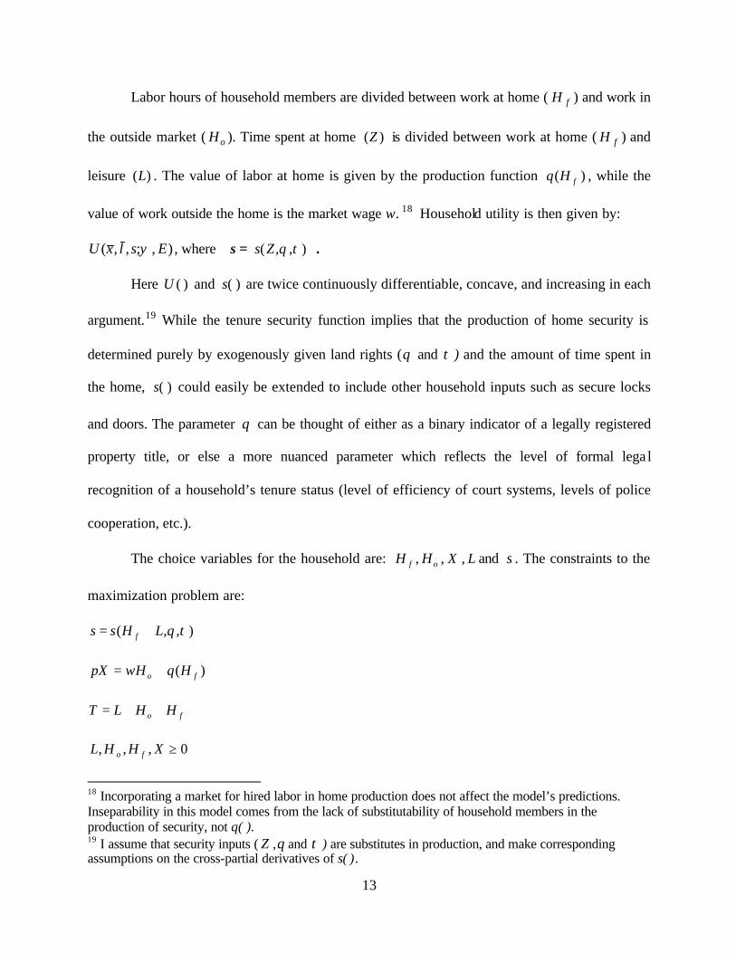
Labor hours of household members are divided between work at home ( fH ) and work in

the outside market ( oH ). Time spent at home )(Z is divided between work at home ( fH ) and

leisure )(L . The value of labor at home is given by the production function )( fHq , while the

value of work outside the home is the market wage w. 18 Household utility is then given by:

),;,,( EslxU ψ , where s = ),,( τθZs .

Here )(⋅U and )(⋅s are twice continuously differentiable, concave, and increasing in each

argument.19 While the tenure security function implies that the production of home security is

determined purely by exogenously given land rights (θ and τ ) and the amount of time spent in

the home, )(⋅s could easily be extended to include other household inputs such as secure locks

and doors. The parameter θ can be thought of either as a binary indicator of a legally registered

property title, or else a more nuanced parameter which reflects the level of formal lega l

recognition of a household’s tenure status (level of efficiency of court systems, levels of police

cooperation, etc.).

The choice variables for the household are: fH , oH , X , L and s . The constraints to the

maximization problem are:

),,( τθLHss f +=

)( fo HqwHpX +=

fo HHLT ++=

0,,, ≥XHHL fo

18 Incorporating a market for hired labor in home production does not affect the model’s predictions. Inseparability in this model comes from the lack of substitutability of household members in the production of security, not q( ). 19 I assume that security inputs ( Z ,θ and τ ) are substitutes in production, and make corresponding assumptions on the cross-partial derivatives of s( ).

14

where )(⋅q satisfies decreasing marginal productivity ( 0>′q , 0<′′q ). Then, normalizing

prices to one, the household’s optimization problem can be written: 20

)),,(),(1

)),(*(1

(max,

τθofofoHHHTsHHT

NHqHw

NU

fo

−−−+

This yields the following necessary first-order conditions for an interior solution

( );0;0 THHHH fofo <+>> :21

oHSlx sUUN

UNw

**1

* += (4.1.1)

lxH UUqf

=* (4.1.2)

Equation 4.1.1 establishes that, at the optimum, households equate the marginal value of

an additional hour of outside labor with the marginal utility of leisure. Equation 4.1.2 states that

they also equate the marginal utility of leisure with the marginal value of an additional hour of

work at home. For each household involved in both home and market work, the solution to this

set of equations implicitly defines demand functions for labor hours in the outside market and in

home production which depend on θ , w, and τ :

),,(** τθwHH ff =→ , ),,(** τθwHH oo =

Assume that 0,0,0 ≤≥≥ sllxsx UUU .22 Then total differentiation yields the following

inequalities for values of w , θ , and τ corresponding to inner optima:

0<∂

∂

θfH

and 0>∂∂

θoH

.

20 For the remainder of the analysis, household characteristics and resource endowment are assumed to be fixed and omitted from the arguments of the utility function. 21 The boundary conditions ∞→

→0llU and ∞→→0xxU guarantee that (Hf + Ho)<T and that at least

one of Hf and Ho is strictly positive. It is shown on the following page that the corner solutions Hf =0 and Ho=0 do not affect the aggregate predictions of the model. 22 Note that this includes the additively separable case, as well as the case in which the value of consumption is rising in tenure security.

15

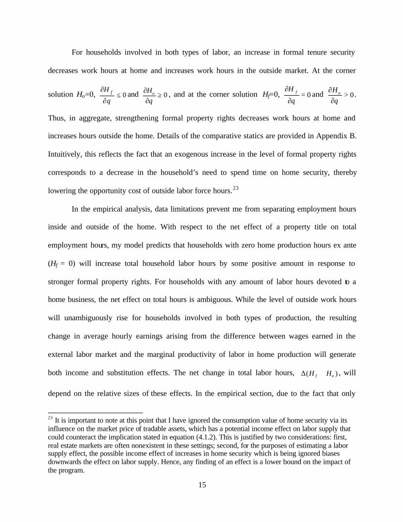
For households involved in both types of labor, an increase in formal tenure security

decreases work hours at home and increases work hours in the outside market. At the corner

solution Ho=0, 0≤∂

∂

θfH

and 0≥∂

∂θ

oH , and at the corner solution Hf=0, 0=∂

∂

θfH

and 0>∂

∂θ

oH .

Thus, in aggregate, strengthening formal property rights decreases work hours at home and

increases hours outside the home. Details of the comparative statics are provided in Appendix B.

Intuitively, this reflects the fact that an exogenous increase in the level of formal property rights

corresponds to a decrease in the household’s need to spend time on home security, thereby

lowering the opportunity cost of outside labor force hours.23

In the empirical analysis, data limitations prevent me from separating employment hours

inside and outside of the home. With respect to the net effect of a property title on total

employment hours, my model predicts that households with zero home production hours ex ante

(Hf = 0) will increase total household labor hours by some positive amount in response to

stronger formal property rights. For households with any amount of labor hours devoted to a

home business, the net effect on total hours is ambiguous. While the level of outside work hours

will unambiguously rise for households involved in both types of production, the resulting

change in average hourly earnings arising from the difference between wages earned in the

external labor market and the marginal productivity of labor in home production will generate

both income and substitution effects. The net change in total labor hours, )( of HH +∆ , will

depend on the relative sizes of these effects. In the empirical section, due to the fact that only

23 It is important to note at this point that I have ignored the consumption value of home security via its influence on the market price of tradable assets, which has a potential income effect on labor supply that could counteract the implication stated in equation (4.1.2). This is justified by two considerations: first, real estate markets are often nonexistent in these settings; second, for the purposes of estimating a labor supply effect, the possible income effect of increases in home security which is being ignored biases downwards the effect on labor supply. Hence, any finding of an effect is a lower bound on the impact of the program.

16

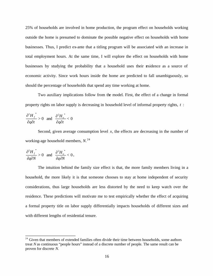
25% of households are involved in home production, the program effect on households working

outside the home is presumed to dominate the possible negative effect on households with home

businesses. Thus, I predict ex-ante that a titling program will be associated with an increase in

total employment hours. At the same time, I will explore the effect on households with home

businesses by studying the probability that a household uses their residence as a source of

economic activity. Since work hours inside the home are predicted to fall unambiguously, so

should the percentage of households that spend any time working at home.

Two auxiliary implications follow from the model. First, the effect of a change in formal

property rights on labor supply is decreasing in household level of informal property rights, τ :

0*2

>∂∂

∂

τθfH

and 0*2

<∂∂

∂τθoH

Second, given average consumption level x, the effects are decreasing in the number of

working-age household members, N.24

0*2

>∂∂

∂

N

H f

θ and 0

*2

<∂∂

∂N

H o

θ.

The intuition behind the family size effect is that, the more family members living in a

household, the more likely it is that someone chooses to stay at home independent of security

considerations, thus large households are less distorted by the need to keep watch over the

residence. These predictions will motivate me to test empirically whether the effect of acquiring

a formal property title on labor supply differentially impacts households of different sizes and

with different lengths of residential tenure.

24 Given that members of extended families often divide their time between households, some authors treat N as continuous “people hours” instead of a discrete number of people. The same result can be proven for discrete N.

17

In addition, testing the entire set of predictions generated by this model allows me to rule

out the possibility that the relationship between tenure security and the utility of consumption is

responsible for the entire effect of property rights on labor supply. As mentioned earlier, greater

tenure security may encourage household members to work on account of an increase in the

value of consumption of immobile assets. While this scenario has similar implications for total

household labor supply, the second-order implication of the model with respect to household size

applies only to the case in which household members’ time at home contributes to home security.

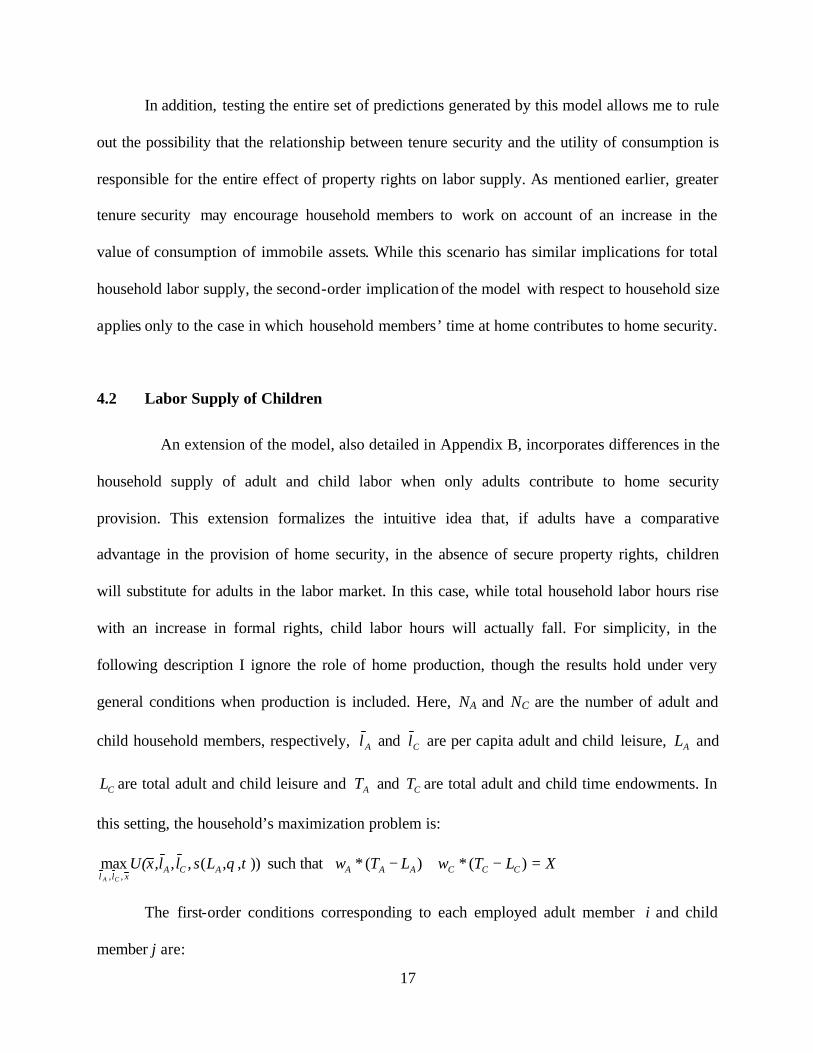
4.2 Labor Supply of Children

An extension of the model, also detailed in Appendix B, incorporates differences in the

household supply of adult and child labor when only adults contribute to home security

provision. This extension formalizes the intuitive idea that, if adults have a comparative

advantage in the provision of home security, in the absence of secure property rights, children

will substitute for adults in the labor market. In this case, while total household labor hours rise

with an increase in formal rights, child labor hours will actually fall. For simplicity, in the

following description I ignore the role of home production, though the results hold under very

general conditions when production is included. Here, NA and NC are the number of adult and

child household members, respectively, Al and Cl are per capita adult and child leisure, AL and

CL are total adult and child leisure and AT and CT are total adult and child time endowments. In

this setting, the household’s maximization problem is:

)),,(,,max,,

τθACAxll

Lsll,xU(CA

such that XLTwLTw CCCAAA =−∗+−∗ )()(

The first-order conditions corresponding to each employed adult member i and child

member j are:

18

0*1

=∗++∗−=AAiA Lsl

Ax

Al sUU

NU

Nw

U (4.2.1)

0*1

=+∗−=CCj l

Cx

Cl U

NU

Nw

U (4.2.2)

From these conditions it can be shown that, for all interior optima, 0>∂∂

θCl and 0<

∂∂

θAl

.

In households in which children are labor force participants, child labor hours will fall and adult

labor hours will rise with an increase in tenure security. For all other households, adult labor

hours will also rise and child labor hours will remain at zero. Thus, given a positive amount of

ex-ante child labor, the aggregate number of child labor hours will unambiguously fall, while the

number of adult labor hours rises with an increase in formal property rights.25

While the theoretical model deals with changes in labor supply at a fixed wage rate, the

empirical model will capture changes in actual employment levels, which are functions of both

supply and demand. Given the size of the program, it is reasonable to anticipate general

equilibrium effects on the wage rate. However, because increased labor supply will decrease the

market wage, as long as leisure is a normal good such effects would only bias downward the

estimated program effect. Thus, the actual labor supply response to titling is presumably higher

than what can be measured with changes in working hours.

25 Although this model focuses on optimal labor allocation, the income effects that follow from relaxing the household’s time constraint provide a plausible alternative explanation for a decrease in child labor with an increase in formal rights, and one that has been proposed by other authors. In particular, a decrease in child labor would follow from the luxury and substitution axioms of the Basu and Van (1998) model of child labor supply, in which children can substitute for adults in the labor market and a family will send children to the labor market only if the family’s income from non-child labor sources falls below some threshold amount.

19

5 Data and Estimation Methods

5.1 Data Set

My empirical analysis of household labor supply responses to changes in formal property

rights relies on the COFOPRI baseline survey data. The sample universe for the survey was all

residences in non- incorporated urban and peri-urban settlements identified in the 1993 census of

the eight cities targeted by the titling program. The data consist of 2750 households distributed

across all eight program cities. The survey was stratified on city, with cluster units of ten

households randomly sampled at the neighborhood level within cities. The number of clusters

drawn from each city was based on the city’s share of eligible residents. The survey instrument

closely mirrors the World Bank Living Standards Measurement Survey (LSMS) in content, and

therefore contains a wide variety of information on household and individual characteristics. In

addition, there are five modules designed to provide information on the range of economic and

social benefits associated with property formalization.

5.2 Identification Strategy

To study the impact of receiving a property title on household labor supply, I exploit

variation in the year in which the COFOPRI program entered a neighborhood to compare

households in program neighborhoods that have already been reached by the survey date to

households in late program neighborhoods. The first step in classifying program timing was to

identify whether or not a neighborhood had been reached by the time of the survey. The survey

data do not directly identify program neighborhoods, nor can this variable currently be

constructed by matching geographic identifiers to COFOPRI office data. Instead, all

observations within a survey cluster are assigned a “program entry” value of one if more than

20

one household in the cluster reports owning a COFOPRI title.26 Clusters in which no household

or only one household have a COFOPRI title are assumed to be those in which the program has

not entered, although it is generally impossible to separate the neighborhoods in which the

program will never enter from those which will be treated eventually. Nonetheless, such

neighborhoods share the key feature of no expected program effect.27 A breakdown of program

and non-program neighborhoods by region is provided in Appendix C.

Not every squatter household that the program reaches is granted a COFOPRI title by the

time of the survey. Reasons that households may be excluded include: the household cannot

prove residence prior to 1995; the household belongs to a cooperative association; the residence

lies on an archeological site, flood plane, mining site or private property; and ambiguous or

disputed ownership claims. Unfortunately, none of the above information is collected in the

survey. 28 Since the households in the treated neighborhoods may or may not actually have

received a government title, this is an intent-to-treat (ITT) analysis.

The second step in classifying variation in program timing was to identify the year in

which the program entered. The effect of the program is presumed to increase over time in a

fashion analogous to a “dose response” measure from the experimental design literature for three

reasons: First, titling an entire neighborhood can be a lengthy procedure, such that the percentage 26 There is clearly some measurement error in this method of identifying treated neighborhoods. In particular, it is possible that nearly all residences in the cluster were not given titles although the program did in fact enter the neighborhood. To address this, I also estimate the model excluding seven clusters in which all sampled households had registered municipal property titles prior to the program, making it impossible to observe whether or not the program entered. In none of my analysis does excluding these 69 households affect the estimate of program effect. 27 Including cluster units with only one reported COFOPRI recipient as non-program neighborhoods does not affect the results. Since it is extremely unlikely that only one household is titled in a program neighborhood several months into the program, such neighborhoods are likely to reflect either misreported title data or recent program entry. If only one household has actually received treatment, effectively the neighborhood is at this stage untreated and neighborhood effects should not be observed. 28 According to anecdotal evidence from program administrators, disputed claims within families or between neighbors are the most common reason that title distribution is delayed for an untitled household in a treated neighborhood (Carlos Gandolfo, personal interview, Lima, August 9, 2000).

21

of titled households within a treated neighborhood increases (at a decreasing rate) over time.

Secondly, household labor supply takes time to adjust. Finally, it is plausible that confidence in

the value of a COFOPRI title is increasing over time. For purposes of exploring the program

effect over time, year of program entry was defined as the earliest reported COFOPRI title year

within the cluster.29 Dynamic response was restricted to be linear in four time periods: January

1999–June 2000, January 1997–December 1998, January 1995 – December 1996, and January

1992-December 1994. This division corresponds to three major waves of program expansion:

From 1992 to 1995, 200,000 titles were granted by the Institute of Liberty and Democracy as

part of a pilot project prior to COFOPRI; the first wave of COFOPRI titles was initiated in 1995

in Lima and Arequipa; and beginning in 1997 the program expanded into six other cities.30

Furthermore, these intervals were consistent with the observed relationship between subjective

statements on tenure security and years since program entry, as is reported for squatters in the

city of Lima in Appendix D. 31

Although target areas for wide scale economic development programs are never

randomly selected, these data have the advantage that all sample members live in areas that will

eventually be targeted for program intervention, increasing confidence in the comparability of

treated and untreated households. Furthermore, the universal nature of the treatment and the

participation rules of the program generally rule out concern over individual selection bias that

29 Due to the fact that not all households were given property titles right away and because of measurement error in title year reporting, households in the same cluster who had received a COFOPRI title did not necessarily report the same title year. When the minimum reported title year fell below the first regional title year according to program data, the second lowest title year was assigned to the cluster. 30 This region-specific pattern of intervention makes it important to include city dummies in regression estimates of program effect. 31 The table in Appendix D reveals a total change in average reported tenure security for residents of Lima of roughly 0.6 points on a four-point scale. The table also illustrates that, while newer households have consistently lower perceived tenure security than more established families, the change in perceived tenure security follows the same approximate trajectory over time since titling program for both groups.

22

could arise even if program placement were random. Nonetheless, there is still potential for

program timing bias, in which areas selected for early program participation are different from

the rest. If program timing is not randomly assigned to neighborhoods conditional on

observables, a comparison of pre- and post-program neighborhoods will produce a biased

estimate of program effect.

The influence of non-random city timing is easily resolved by including city fixed effects

in the regression estimates.32 A more complicated source of program timing bias concerns the

order in which project teams entered neighborhoods within cities. Empirical evidence that this is

not a relevant complication is provided from a comparison of early and late neighborhood

characteristics prior to the program. Table 1 reports district level poverty indicators from the

Peruvian Ministry of Economics and Finance based on 1993 census data. The last row reports the

general poverty indicator constructed from a weighted mean of eight district- level measures,

reported in the rows above: rates of chronic malnutrition, illiteracy, fraction of school-aged

children not in school, residential crowding, adequacy of roofing, and the proportion of the

population without access to water, sewerage, and electricity. 33 Not only is the general poverty

index similar across program and non-program neighborhoods in 1993, but the differences in all

eight base indicators reported in the rows above are small and insignificant, and vary in sign

across indicators. The observed similarity between program and non-program neighborhoods in a

32 The only information on the ordering of cities comes from a vague statement in the World Bank Project Report (#18359), which specifies that the order was designated in advance according to “ease of entry.” As far as neighborhood program timing, there appears to have been no specific algorithm in the program guidelines. The COFOPRI office claim only that order was subject to “geographical situation, feasibility to become regularized, dwellers’ requests, existing legal and technical documents, and linkages with other institutions involved in the existing obstacles” (Yi Yang, 1999). 33 Higher values of the index reflect higher poverty. For a detailed description of how the FONCODES indicator was constructed, see Schady (2002).

23

range of poverty measures is strong evidence against all obvious sources of endogenous

neighborhood program timing within cities.

Further evidence that program timing was independent of neighborhood economic

development comes from a visual inspection of the entry patterns of the titling program in Lima,

the only program city in which all four waves of program expansion are represented. Figure 1

plots the basic progression of land titling through districts in Lima as reported in my sample. In

general, program activity begins in the city center (during the ILD period), then moves to the

perimeter of the city and gradually spreads back into the city center. The spatial pattern of

poverty in Lima according to 1993 poverty indicators appears entirely unrelated to program

timing patterns. According to the corresponding poverty map in Figure 1, Wave 3 (1997-1998)

and Wave 4 (1999+) program activity takes place in districts that span the entire range of poverty

levels (1-4). Wave 1 (1992-1994) activity, which took place in the center of the city, covers

districts spanning poverty levels 2-4, while Wave 2 (1995-1996) takes place in districts ranging

in poverty level from 1-3. Worth noting is the fact that when the government took over the titling

program during Wave 2, program activity in Lima was initiated simultaneously for political

reasons in each of the three regions of peri-urban settlements, shown by the white squares on the

map. Thus, in waves 2 and 3, program activity is spread across districts from the Southern,

Northern, and Eastern Cones of Lima.

While the available information on program timing suggests that is was largely

exogenous to the economic environment of neighborhoods, without precise knowledge of the

formula for neighborhood timing I cannot safely assume random assignment to treatment nor

accurately specify a selection on observables model. Hence, cautious quasi-experimental analysis

calls for an estimation strategy that is robust to potential selection on unobservables.

24

To reduce the role of endogenous program timing, my identification strategy makes use

of a comparison group of non-beneficiary households. In a framework analogous to difference-

in-difference (DID) estimation, I compare the difference in labor supply of potential program

beneficiary and non-beneficiary households in neighborhoods that the program has reached to

the difference in neighborhoods that have not been reached. The simple idea underlying this

distinction is that the tenure security effect of titling disproportionately (or solely) benefits

households with weak ex ante property claims, for whom the demand for tenure security is

high.34 To capture this, I make use of detailed survey data on past and present property titles to

construct a binary indicator of whether or not a household had a title at the start of the titling

program. Those who do not are labeled “squatters,” while the term “non-squatter” refers to

households with pre-program titles. 35

While the labor supply of squatters may systematically differ from that of non-squatters

due to any number of unobservable factors, identification of program effect will be robust as

long as this behavior is constant across program and non-program regions. To address the

possibility that it is not, I take two additional steps. First, I control for a large set of observable

household and neighborhood characteristics in an effort to capture exogenous differences in

household types between program versus non-program areas. Nonetheless, the conditional

independence assumption will still be violated if there exist patterns across program and non-

program neighborhoods in a relevant unobserved characteristic that affects the economic

34 There were several ways a household might have obtained a property title in the era before the recent titling effort. First, there was always the lengthy and costly option of following the official bureaucratic process for obtaining and registering a municipal property title. Second, there were a handful of past isolated attempts at property reform in which interim titling agencies were set up by munic ipal governments in an effort to incorporate some proportion of informal residents (De Soto, 1986). Finally, on a number of occasions, mayoral and presidential candidates were known to distribute property titles in an effort to win voter support prior to an election (Yi Yang, 1999). 35 Throughout this paper, “squatter” will refer to households lacking property titles prior to the program.

25

environment of squatters differently than non-squatters. As a further step, I exploit two sources

of predicted variation in the impact of the treatment on different households types. As implied by

the model of Section 4.1, I expect the impact of receiving a title to be decreasing in both the

number of working age members and the level of informal property rights. This allows me to

additionally estimate models that test for predicted heterogeneity in response to the program

according to household size and residential tenure.. Residential tenure is used as a summary

measure of a household’s level of informal property rights. This stems from the assumption that

households with longer community membership can rely more heavily on community

enforcement, documented in studies on informal property protection such as Lanjouw and Levy

(2002) and De Soto (1986). Furthermore, aside from reflecting community ties, length of

residence could enter positively into home security by lowering the household’s uncertainty

about eviction likelihood.

Because both household size and residential tenure are highly correlated with poverty but

in opposite directions, the dual restriction that program effect be increasing in household size and

decreasing in residential tenure heavily reduces concerns over program timing bias by

eliminating the possible confounding role of any unobservable trends that are correlated with

household poverty. 36 In order for a regional trend in some unobservable determinant of labor

supply to be mistakenly attributed to the program, its influence would have to be decreasing in

both residential tenure and household size, and hence no such factor could be correlated with

poverty in either direction.

Table 2 provides descriptive statistics on the sample population, allowing an informal

check for random assignment of program timing. As the means in the table indicate, there is

36 Correlations between a 3-level poverty index and household size and length of residence verify these patterns in the COFOPRI baseline survey data.

26

variation in some demographic characteristics across program and non-program regions.

Namely, sample households in program areas on average have smaller dwellings (fewer rooms),

are more likely to have electricity, and have higher nativity rates (percentage of members born in

province). However, while statistically significant differences exist across program and non-

program areas, no statistically significant differences in differences are observed between

squatters and non-squatters in program and non-program areas (column 3). This finding supports

the use of non-squatters as a comparison group.

5.3 Regression Model

The basic estimate of program effect is obtained from the following OLS regression:

Li = ß0 + ß1(N) + ß2(N)2 + ß3(squatter) + ß4(program) + ß5(program*squatter) + a´Xi+ei, (5.3.1)

where Li refers to some measure of household labor supply; N is number of household

members; squatter refers to a household with no pre-program property title; program indicates

whether the household lives in a neighborhood that has been reached by the program; and Xi is a

vector of demographic controls. The coefficient on the interaction between program and

squatter, ß5, is the estimated program effect, which provides a measure of the conditional (on Xi)

average difference in time worked by ex-squatters in program areas versus non-program areas.

The inclusion of controls for squatter and program fixed effects corresponds to a standard DID

empirical specification.

The second estimate incorporates a gradient of the program effect over time.

27

Li = … + ß6(program periods) + ß7(program periods*squatter) (5.3.2)

Here, the variables of interest are the interactions between the dummy variables for

squatter household and program entry, ß5, and between the squatter dummy and the number of

periods since the titling program entered, ß7. Together, these pick up any differential patterns in

labor supply of squatters relative to non-squatters that are consistent with the neighborhood’s

years of program experience. The combination of these interactions, ß5 + ß7(mean # program

periods), is the estimated average program effect. This can be interpreted as the marginal change

in the amount of labor supplied by the average squatter household in a program neighborhood for

each additional period with a property title.37 Additional variation in program response by

residential tenure and household size is captured by the following models:

Li = … + ß8(tenure) + ß9(tenure*squatter) + ß 10(tenure*program) + (5.3.3) ß11(tenure*program*squatter)

Li = … + ß12(N*squatter)+ß13(N*program) + ß14(N*squatter)2 + ß15(N*program)2 + (5.3.4) ß16(N*program*squatter) + ß17(N*program*squatter)2

The variable “tenure” in equations 5.3.3 and 5.3.4 refers to the number of years a

household has lived in a residence, which is used as a summary measure of household informal

rights and corresponds to τ in the theoretical model. In (5.3.3), the average program effect is

37 The validity of the linear constraint on the program effect across periods of program entry is tested by running unconstrained versions of the regressions for all outcome measures, presented in Appendix E. In these models, instead of the interaction term squatter*(program period), four dummy variables are included corresponding to each period of program entry such that the slope of the program effect is not constrained to be linear over time. The coefficient estimates reveal a strikingly consistent trend of increasing program effect over number of periods since the titling program began, supporting the use of a linear restriction. For all outcomes, adjusted Wald tests fail to reject the hypothesis that the differences between program periods are equal (and therefore that the slope of the program effect is linear). Furthermore, the estimates in Appendix E reveal the necessity of allowing for a level effect of the program that is larger than the period-to-period program effect for all outcomes except in-home work.

28

captured by [ß5 + ß7(mean # program periods) + ß11(mean residential tenure)], while in (5.3.4)

the estimated average program effect is [ß5 + ß7(mean # program periods) + ß11(mean

residential tenure) + ß16(mean household size) + ß17(mean HH size)2]. The quadratic term in

(5.3.4) captures the idea that leisure hours are likely to be correlated across household members,

such that the likelihood that any household member is at home in a given moment is increasing

with family size at a decreasing rate. All estimates are adjusted to account for the sample clusters

and strata, the standard errors derived from the Huber-White robust estimator for the variance-

covariance matrix. 38

The set of regressors contained in Xi is common to all regressions in the empirical

section, and includes controls for the number of working-aged household members, city fixed

effects, lot size and residential tenure, as well as a constant. In addition, Xi includes the following

demographic controls: sex, age, education and degree level of household head; number of

household members, number of school-age children, number of babies (ages 2—4), fraction of

adults that are male, fraction of adults that are immigrants (born outside of province), and

number of members age 70 and older; size of property, household residential tenure, whether

indoor plumbing, whether the property was acquired by invasion, and whether the property was

inherited; whether dwelling lies within walking distance of nearest primary school, secondary

school, bus stop, public phone, and public market, and this indicator interacted with walking time

to each locale; and whether neighborhood has local bus stop/market/public phone/primary and

secondary school currently and whether each of these existed two years ago, and whether

neighborhood has government school, child, food or general social assistance program.

All regressions also include a set of dummy interactions between cities and program

entry, and between cities and pre-program title status. The inclusion of these interactions absorbs 38 For a description of the technique used to estimate standard errors, see Chapter 2.2 of Deaton (1998).

29

potential regional variation in program implementation and regional differences in informal

property institutions that could be driving relative differences in program impact between titled

and untitled residents. It is arguable that the inclusion of such a wide set of demographic controls

amounts to over-controlling. However, as detailed in Appendix F, all of the proceeding results

are robust to the exclusion and inclusion of a wide variety of right-hand-side variables. For all

outcomes in Section 5, coefficient estimates from regressions with no demographic controls are

presented alongside the saturated models.

5.4 Endogeneity Concerns

With respect to the choice of right-hand-side variables, while an effort was made to

include principally time- invariant household characteristics, there remain many sources of

potential endogeneity in the set of regressors. Most notably, endogenous migration of household

members, fertility and housing investment are all behaviors arguably correlated with tenure

security. The robustness of regression estimates to a wide range of specifications provides

general evidence against the role of endogeneity bias (see Appendix D). With respect to

investment, increased credit opportunities among post-program squatters should only bias

downward the estimated program effect, given that greater ability to smooth income has the

potential to lower the marginal utility of wage income, thereby reducing the opportunity cost of

leisure. Furthermore, credit has the potential to increase educational investment, an additional

pull factor reducing employment hours in post-program areas. Nonetheless, in order to minimize

endogeneity concerns, only lot size and underground residential infrastructure are included

30

among the characteristics of the residence, both of which are reasonably believed to be relatively

time- invariant.39

The potential endogeneity of credit access generates one notable complication in

interpreting the home business outcome only. Namely, it is possible that the untitled are

sufficiently credit constrained to be unable to cover the fixed cost of moving a business from

inside to outside the home (this would apply to non-self-employed as well if labor force

participation involved a high enough fixed cost of participation). However, this is inconsistent

with corresponding sample data on business loans, as well as evidence from four separate studies

of credit effects of COFOPRI, in which property titles were found to have no significant effect

on residents’ access to business credit (Field and Torero, 2002; Cockburn, 2000; Kagawa, 2001;

Torero, 2000).

Individual sample selection arising from household migration is unlikely to be a relevant

complication in this analysis due to the fact that is was widely known that new residents were

ineligible for a property title. Migration of individual household members, however, could

complicate the analysis if non-random migration rates differentially altered family composition

of treatment and control groups. The principal evidence that this is not the case comes from

direct comparisons of treatment and control group data on residency of household members,

recent migration of past members, number of working-age members, and age and sex of

household head, none of which reveal significant differences in family composition. As fertility

is potentially influenced by changes in tenure security, children under age two are excluded from

right-hand-side measures of family size.

39 A 2000 study of a sample of COFOPRI participants by Kagawa revealed that residential levels of sub- terra infrastructure, and in particular the public water connection system, does not systematically vary with neighborhood regularization (Kagawa, 2000).

31

A final source of potential endogeneity bias arises in all experimental and quasi-

experimental settings in which participants are aware of treatment. In particular, program timing

would not identify the treatment effect of obtaining a title if the control group adjusted their

behavior in anticipation of treatment. Anecdotal evidence from COFOPRI office personnel

suggests that there was much uncertainty as to the timing and choice of program locations,

making it is unlikely that households would feel confident in advance that the program would

eventually enter their vicinity.40 More importantly, this behavior would only bias downward the

estimated program effect in my model. The only possibility for upward biases is an “Ashenfelter

dip” response of future program participants, in which squatters spend disproportionate time

safeguarding property when the program is about to enter. While possible, there is no intuitive

nor anecdotal reason to expect demand for invasions to rise in anticipation of the program.

6 Empirical Results

6.1 Program Effect on Tenure Security

The theory of Section 4 posits that obtaining a property title affects household labor

supply by increasing tenure security. Naturally, if becoming a titled property owner does not

change households’ perceived probability of eviction, there will be no expected program effect.

Survey data on household perceptions of eviction likelihood are therefore informative for

verifying the presumed relationship between title acquisition and tenure security before

continuing with the analysis. The following indicators are explored: whether the household

reported experiencing a change in tenure security with the acquisition of a property title, whether

eviction is considered “very likely” and whether eviction is considered “very unlikely.” Indeed,

40 Interview with Carlos Gandolfo, COFOPRI Office, Lima, Peru, August 2000.

32

according to the simple DID estimates in Tables 3a–3c, the data provide evidence of a basic

program effect that is consistent with the variations in program entry and groups of beneficiaries

described above. Squatters in program neighborhoods report significantly higher current levels of

home security (3a, 3b) and changes in tenure security associated with property titles (3c). Thus, it

is reasonable to conclude that the program indeed led to significant increases in tenure security.

6.2 Reduced-form Estimates of Effect on Labor Supply

Strong evidence of a corresponding program effect on household labor supply comes

from a visual comparison of pre-program squatter and pre-program titled households in program

and non-program neighborhoods. Figure 2 plots the distribution of annual labor force days per

household worker by these four sub-samples.41 The density marked by squares, which

corresponds to squatters in neighborhoods not yet reached by the program, is visibly distinct

from the densities corresponding to the two groups of residents in program areas and also from

that of the titled residents in non-program areas. Two important patterns are worth noting: First,

among non-squatters, the employment hours distribution of residents across program regions is

very similar, whereas among squatters the distributions depend heavily on whether or not the

program has entered.42 Second, not only are the work patterns of the comparison group relatively

constant across program and non-program areas, but they are also similar to the work patterns of

pre-program squatters after the program has entered. These regularities lend confidence to the

use of non-squatters as a comparison group. The program effect interpretation of such a picture is

that the titling program leads squatter households to shift outward their distribution of work

41 While my empirical estimates will focus on weekly and not annual hours worked, the patterns reflected in Figure 2 is useful in providing the clearest illustration of my identification strategy. 42 In fact, the hours distribution of squatters in program areas stochastically dominates that of squatters in non-program areas.

33

hours to reach that of title-holders, as would occur if lack of tenure security were responsible for

the employment hours differential.

To further explore this pattern, a linear regression framework is needed to control for

household, neighborhood and regional determinants of labor supply which, if unbalanced, could

confound measures of program impact. Tables 4—6 present the coefficient estimates of interest

from models (5.3.1)—(5.3.4) of Section 5.3. Column 1 reports results from the sparsest

regression, which constrains the program effect to be constant across household type and time

since titling, while columns 2, 3 and 4 allow the program effect to vary by time since program

entry, length of residence and family size, cumulatively. The outcomes of interest are total

household weekly hours of work, total household annual months of work, and fraction of

household members in the labor force.43 Weekly hours of work refer to last week’s employment,

and is constructed from survey questions on the number of days and mean hours per day worked

last week asked of all household members who report having worked during the past week.

Working-age members who are not in the labor force and those who are in the labor force but

report not having worked last week are assigned employment hours values of zero. Annual

months of work is constructed from survey questions on the number of months worked of the last

twelve, asked of all household members who report having worked during the past year (which 43 In total, 99 households are dropped from the analysis due to missing labor supply information (a household is considered to have missing weekly hours data if it has one or more members who both report having worked last week and have positive reported values of either hours worked per day or days worked per week and missing values of the other variable), 31 households have missing data on property size and/or local elementary school facilities, 20 households are excluded in two clusters in which program entry does not match institutional data on regional program timing, and 8 households are excluded because all members are reported as over the age of 80, leaving a total of 2592 households. Due to the survey design, information on daily and hourly work time was incomplete (but not missing) for 69 individuals who reported not working in the last week but working over the last twelve months. For such individuals, only the number of months out of the year worked was asked, and not days a week or hours a day worked. For the weekly hours variable, these individuals are assigned values of zero for days worked last week and hours worked last week. For the annual hours estimates in Figure 2, predicted values of hours and days a week were assigned to these observations based on a vector of household and individuals characteristics. No predicted values, however, were used in the regression or probit estimates.

34

includes all those who worked last week).44 Labor force participation is measured as the fraction

of working-age household members who report either having worked, had a temporary absence

from the labor force or searched for a job during the past week.

In column 1 of Table 4 the marginal effect implied by the estimated coefficient on the

interaction term between squatter and program is roughly 13.4 hours per week. In column 2,

which allows the program effect to increase with time since the program began, the marginal

effect implied by the estimated coefficient on the interaction term between squatter and program

periods is roughly 14.5 hours per week, while the fixed effect is -12.7 hours but insignificant.

This implies a total program effect of roughly 16.2 hours per week for the median squatter

household with two periods of property rights. For the average househo ld without a property

title, this implies a 17% increase in total household labor supply per week – or around two days

of full- time work. The long-run or “steady state” effect of the program reflected in the estimated

effect on households with the maximum number of program periods, is an average increase of 45

hours of employment per week across the entire target population of squatters – roughly the

same as one full-time worker being added to the labor force.

For “new” households and households with few working-age members, the program

effect is even larger. The estimates in column 3, in which the program effect is allowed to vary

by residential tenure, provide evidence that newer residents increase labor hours more in

response to an increase in tenure security. In the regressions that account for differences

according to household years of residence, the estimated program effect rises to 22.6 hours per

week for the average squatter family with 15 years of residential tenure – a 23% increase in

household labor supply. Furthermore, allowing the program effect to vary by residential tenure 44 Unfortunately it is impossible to combine months and hours responses to create a summary measure of annual labor supply without using predicted values of weekly hours for people who worked last year but not last week.

35

accounts for the negative coefficient on the main effect of the program in column 2. When the

program effect is allowed to vary by family size, we observe even stronger evidence that the

impact of the titling program on labor supply is concentrated among households with few

potential workers. In column 4, when both sources of variation in treatment response are taken

into account, both the level effect and the “dose” effect of the program become significant.

Although the estimated effect on the average squatter household falls to 12.3 hours and becomes

insignificant, the estimates indicate that the size of response depends heavily on household type.

Thus, small families and families with few years of residence account for the majority of the

program effect captured in columns 1–3.

As mentioned in Section 4, the column 4 patterns of heterogeneity in program response

according to residential tenure and family size provide additional evidence that unobservable

factors are not biasing the results. While poverty and program effect should decrease with

residential tenure, poverty and program effect move in opposite directions with respect to

household size. Thus, any unobserved heterogeneity between early and late program

neighborhoods that is correlated with poverty level could not be responsible for both patterns of

variation in program influence.

To explore in more detail how the program response varies by households size and

residential tenure, Table 4a presents the estimated program effect for a range of household types.

At least two things are worth noting from this chart. First of all, the program effect does not

appear to “kick in” until more than a year after the first title is distributed. This could be driven

by the fact that titling within a neighborhood takes an estimated eight months to complete, such

that a disproportionate number of households in the most recent program regions are still untitled

36

by the time of the survey.45 Alternatively, this could reflect an adjustment lag necessary for

households to either re-optimize labor supply or to ascertain the increase in tenure security

associated with their newly acquired land title.

Secondly, the program effect falls with family size only for households with less than

five workers. As shown above, the quadratic function estimating the program effect according to

family size reaches a minimum at five working-age members, at which point the estimated

program effect remains well above zero. This is inconsistent with the model of Section 4, in

which, as long as it is significant, the program effect falls with household size, in which case the

minimum of the quadratic function should not be bounded away from zero additional hours.

Instead, the results above suggest a model in which either desired leisure time per capita falls

(equivalently, desired consumption per capita increases) with household size, or else the demand

for tenure security increases with household size (as opposed to the model’s assumption that

security demands are independent of number of members, controlling for lot size, residential

tenure, and formal rights). Most likely, the second association is responsible on account of

unobserved heterogeneity in household type correlated with household size.

As reported in Table 5, the effect of the titling program on total household months of

work tells a similar story to the estimates on weekly hours. The measured program effect on

household annual employment months is approximately 2.9 months, slightly less than the month

effect implied by the weekly hours estimates. Differences between the sizes of the program

effects reported in Table 4 and Table 5 largely reflect the extent to which reductions in labor

supply driven by tenure insecurity are due to shorter average work weeks versus extended

45 Time estimate reported in a mimeo on the program procedure distributed by the COFOPRI office in Lima.

37

periods of unemployment or non-participation. Thus, the combined estimates suggest at least

some increase in the number of labor force participants.

Indeed, Table 6 reveals that added workers account for a significant portion of the change

in family labor supply resulting from the titling program. When the same regressions are run on

household labor force participation rates, we observe an implied 6–7 percentage point increase in

the number of working-age household members who are employed or searching for work

(columns 1 and 2). With an average 49% labor force participation rate among squatter

households with four working-age members, an effect of this size would be accomplished if one

in every four households that obtains a property title adds a worker to the labor force (25%/4 =

6.25%). Even if every such added worker worked full time (48 hours per week), additional labor

force participants could not account for the entire implied program effect on hours. This suggests

that average hours of the employed are also higher among program participants. As evidenced in

Figure 2, a rough comparison of average hours per worker reveals a difference in the average

number of employment hours of workers in program areas and non-program areas of around 5

hours per week. In the average two-worker (four-member) family, this accounts for

approximately two-thirds of the program increase in hours.

Table 7 decomposes by gender the program effect on hours to study separately the impact

of titling on work hours of adult men and women. The regressions in columns 1 and 4 of Table 7

are identical to the column 1 and 4 regressions in Table 4 except that further controls for family

composition are included (number of adult men, adult women, boys and girls aged 12–16, and

children aged 5–11). Furthermore, to reduce the dimensionality of the program effect for

analytical purposes, in all Table 7 regressions the program effect is constrained to be constant

38

over time.46 The estimates reported in columns 1–3 indicate that changes in male employment

account for the majority of the program effect on hours. In column 2, we see that higher male

hours account for 10.3 out of the implied total program effect of 12.9 hours. Meanwhile, the

difference in female hours (column 3) is small and insignificant. However, not surprisingly,

female hours are much more elastic than male hours. Although the mean effect of acquiring a

property title on hours worked by women is close to zero and insignificant for the average

family, when the program effect is allowed to vary with family size and residential tenure, we

observe that the effect on female hours depends heavily on household type. For instance, in

families with only two working-age members and ten years of residence, the implied program

effect on female labor is 18.2 additional hours per week and statistically significant. This is

equivalent to one in three women joining the labor force full time. In contrast, as observed in

column 5, the average program effect on male hours does not depend on either family size or

length of residence.

6.3 Effect on Child Labor Force Participation

As motivated by the model of in Section 4, an increase in formal property rights is

predicted to generate a decrease in the amount of child employment if children have a

comparative advantage in market work relative to home security. The next set of estimates looks

for an effect of property titling on child labor force participation. In the sample, only 8.2% of all

households report regular labor force participation (excluding unpaid domestic work) by children

46 When working hours of men and women are regressed separately on the level effect and the does response, (program periods)*squatter, it appears that female hours change initially but do not rise over time, while male hours change less initially but gradually increase with additional years post-program. The discrete change in female hours suggests that female workers are likely to be new labor force entrants, whereas men are more likely to be old labor force participants increasing hours of work over time.

39

between the ages of five and 16. This fraction could easily underreport the actual level of work

hours by children, as households might be reluctant to admit to children working or not consider

irregular employment of children when answering survey questions. Yet, while this number is

low, it is not clearly underreported. According to International Labor Office estimates, 4.1% of

all Peruvian children aged 6—14 were economically active in 1993. Though the rate should be

higher for the relatively poor households in my study, it is also true that urban households have

lower rates of child labor than do rural households in Peru (Ray, 2000).

To study the effect of urban property titling on child labor, I estimate a probit model

where the dependent variable is a dummy indicator of whether or not any household members

under age 16 are reported as working more than five hours per week. I estimate a binary model

rather than modeling the marginal effect on child labor hours due to the fact that the majority of

families report no child labor hours, necessitating a limited dependent variable model with more

stringent functional form assumptions. Table 8 reports the coefficients and marginal effects from

the probit estimates with a full set of controls.47 Column 1 estimates the program fixed effect on

child labor, where the coefficient on the interaction term is analogous to the DID strategy in a

linear framework. Columns 2 and 3 decompose the program effect across households of different

sizes, first allowing the program effect to change linearly with household size, then by measuring

the program effect on only the smallest 85% of households.

While the first column shows no average program effect on the probability of children

working, when the effect is allowed to vary by family size, we observe a significant effect of

property titling on households with fewer than four working-age members. As reported in

column 2, for households with three working-age members, the implied marginal effect of 47 In an effort to avoid mistaking young domestic workers for children, I exclude single male -headed households. Including these households lowers the point estimate of program effect slightly but the estimate remains significant.

40

property titling is large (2.4 percentage points, where the mean is 7.8%) and significant. For

larger families, the effect is close to zero and insignificant. This is consistent with the theoretical

predictions and with the estimates of Table 4: if families with more than four working-age

members are unconstrained by the need to keep family members at home, neither should they

have incentive to send children to work in place of adults.

To estimate the average program effect on constrained households and also test for

potential non- linearities in the family size effect, I also run the same model excluding the largest

13% of households in the sample, those with more than six working-age members. Coefficients

from this model are presented in column 3. When families with many potential workers are

excluded, we observe that obtaining a property title reduces the average likelihood of children

entering the labor market by 2.2 percentage points. According to this estimate, the implied

program effect on child labor force participation among families with 1–6 working-age members

amounts to a reduced likelihood of roughly 28%.

While the estimated impact of property titling on the probability of children working is

compelling, the mechanism by which property rights reduce child labor is ambiguous. If child

leisure is a normal good, the prediction would also follow from the income effect of an increase

in adult wage earnings due to added work hours. Both explanations are consistent with past

research on the determinants of child labor force participation in Peru, in which it was found that

child employment levels are responsive to changes in the adult male wage (Ray, 2000). While

property titling does not necessarily generate an increase in the adult wage, an analogous result

should arise from a change in the opportunity cost of adult leisure, which in this model is the

wage minus the security value of leisure.48

48 I observe no significant effect of titling on the probability of child schooling. This is consistent with evidence from past studies on child schooling and employment in Peru, which found schooling levels to

41

6.4 Effect on Rate of In-home Work

The final question addressed in this paper is whether or not members of a household

participate in market work at home. In the sample, 24.3% of households report running a

business from home.49 While a general class of models of household production treat labor

supply decisions as separable from production decisions, in my model, in-home work has the

additional feature of increasing tenure security and thereby reducing the household demand for

leisure. Thus, in the absence of a property title, the model implies that the decision to run a

business from home is determined jointly with decisions about the total number of hours worked

by household members. According to the predictions of Section 4, the marginal value of in-home

work falls when formal property rights are secured and there is no longer a security incentive to

stay at home. As a result, newly unconstrained decision-makers will have incentive to more

efficiently allocate resources by moving production outside of the home or finding work with an

outside employer. The nature of this relationship between business investment and land titling is

a surprising departure from the rural context, in which land titles are hypothesized to promote

investment in home production (Besley, 1995). Given the amount of attent ion paid to increasing

credit access via land titling programs, it is interesting to note that investment demand in the

urban case may actually fall with increases in tenure security if increased worker mobility causes

the rate of self-employment to fall.

The probit estimates presented in Table 9 support the theoretical prediction. In column 1,

the marginal effect implied by the coefficient on the interaction term between squatter and

be unresponsive to child labor due to the country’s high percentage of working children who are also enrolled in school (Ray, 1999). 49 The exact survey question is: “Do you participate in some economic activity within your home or use part of your property as a source of economic activity?”

42

program periods is a 7.6 percentage point reduction in the likelihood of owning a home business

for the average squatter household, though the estimate is not significant. However, when the

program effect is allowed to increase over time, the implied program effect rises and becomes

significant. In column 2, the implied margina l change in the likelihood of working inside the

home falls by 11.6 percentage points for the average squatter family with two program periods –

implying a reduction in the rate of home business activity of approximately 47%. Interestingly,

as shown by the coefficient estimates in column 3, the program effect on in-home work does not

appear to depend heavily on family size or residential tenure, a possible indication of omitted

variables bias or other specification error.

As an additional test of variation in program response in which the covariates are not

assumed to be constant across household types, I run the probit estimate separately for

households living on properties acquired by invasion of first resident (32% of sample) versus

non- invaded properties (purchased, inherited, or acquired by some other transfer).50 Households

on invaded properties generally suffer from acute tenure insecurity, and are therefore presumed

to have higher demand for a property title. Coefficients from this estimate are reported in the last

column of Table 9. As expected, the effect of obtaining a property title on the decision to operate

a home business is much more severe for the sample of invaded properties and insignificant for

all other residents. In fact, the estimated coefficient for relatively insecure households is more

than six times the size of the coefficient for all other residents. The sub-sample of invaded

residences also exhibits the familiar pattern of program response by residential tenure and

household size. In contrast to the differential effects on in-home work, the program effect on

50 The expected trends were also observed in comparisons between other sub samples, including male versus female household heads and households with and without children.

43

labor hours does not differ substantially according to whether the household was acquired by

invasion. 51

This combination of labor supply and business location responses suggests a more

complicated model of household labor supply and tenure security. The differential impact of the

home business result for families on invaded properties is consistent with a story in which very

insecure households whose security needs require a larger amount of time spent at home and/or

very poor households with little disposable income feel particularly constrained by the amount of

foregone earnings home security provision entails. Given the alternative to work inside the

home, such families choose to reduce total work hours only up to a point after which it is more

beneficial for household members to shift production inside the home rather than substitute

leisure for outside work hours. This would explain why the home business effect is only

observed among very insecure households, whereas the labor hours effect is universal. 52

6.5 Robustness Checks

To lend support to the previous set of estimates, I use propensity score matching based on

the probability of residing in a program neighborhood to construct a comparison group of

untitled residents of non-program areas. Propensity score matching reduces bias created when

51 Nonetheless, the total program effect on invaded households is substantially larger than it is for non-invaded households, since this population experiences both an increase in hours as well as a shift from production inside the home to production outside of the home. 52 Further evidence of the home business effect is provided by a comparison of the average ages of home businesses before and after the titling program. If the implications of Table 10 on in-home work fit the proposed model, not only should the frequency of home businesses be lower but also the average age of home businesses should be higher among squatters after the titling program. Given that households on invaded properties appear to account for the vast majority of the estimated program effect on rates of in-home work, the estimates are run separately on the sub samples of invaded and non-invaded households. Indeed, we observe that home businesses located on invaded properties are an average of 6.3 years older in program regions than in non-program regions. For home businesses located on non-invaded properties, the age difference is small, positive and insignificant.

44

the linear model underlying regression adjustment is incorrect. For comparability with the OLS

estimates, the same covariates are used to derive the predicted probability of a neighborhood

being reached by the program in a probit estimate. As reported in Table 10, average treatment

effects based on kernel matching on the predicted z-score replicate the pattern of program effects

found in the OLS estimates in both magnitude and pattern of program impact according to

household size.53 The estimated labor supply response to obtaining a property title is 12.3

additional hours of work, a 5.1 percentage point increase in the fraction of working-age

household members in the labor force, and a 9.1 percentage point decrease in the likelihood of

running a business from home. When the labor hours result is broken down by household size,

the estimated average effect of a property title is 14.2 weekly hours among household with less

than four members, 7.2 hours among households with 4—5 members, and insignificant among

households with more than five potential workers.

As an additional robustness check, I run identical estimates on the sub sample of

households that are ineligible for receiving a title on account of having moved into their current

residence post-1995. Clearly, if property titles are responsible for the observed change in labor

supply, we should observe no program effect among ineligible residents.54 Indeed, there is no

measurable program effect on ineligible households (in fact, the estimated program effect is

negative, though insignificant), which is particularly compelling given that newer households

tend to have very low tenure security. Finally, the previous results are robust to several

alternative definitions of “squatter.” For instance, altering the definition of squatter to include

households with unregistered municipal titles actually increases slightly the predicted effect. In

addition, excluding Lima from the analysis produces the same pattern of coefficients, but with

53 Nearest neighbor and stratified matching produce a similar pattern of outcomes. 54 While ineligible residents could serve as a control group, too few (9.4%) are identifiable in the data.

45

much larger standard errors. The mean ITT effect is smaller, which is accounted for by the lower

rate of titling in newer program areas.

7 Long-Run Predictions

Given the size of short-run effects of the COFOPRI program, it is interesting to consider

the scope of impact of the nationwide titling effort. Based on the previous estimates, what is the

change in labor supply that a program neighborhood would experience once all eligible squatters

have been titled and the total increase in perceived tenure security and adjustment lags have

occurred? Two challenges arise in predicting the average treatment effect on titled households

after several periods with a title from the current set of estimates. In particular, the results

presented in Tables 4–6 underestimate the long-term impact on labor supply because both the

rate of titling and the impact of titling within a program neighborhood presumably increase over

time. The first complication arises from the ITT nature of the identification strategy, which is

analogous to non-compliance in experimental data. The fact that it is impossible to observe in

pre-program neighborhoods whom among the eligible would promptly receive a title upon

program entry makes it necessary to include all eligible recipients in an ITT analysis. A

disadvantage of this strategy is that it fails to isolate the program effect on the households that

actually received a title through the government program and therefore underestimates the long-

term impact of residential formalization. While 74.2% of squatters in titled neighborhoods did in

fact receive a registered government property title by the time of the survey, the inclusion of the

remaining 25.8% of untitled program participants biases downward the estimate of program

effect. The second complication is that the previous results average the short-term effect on

newly titled households with the long-term effect on households titled many years ago. If the

46

security gains from receiving a title increase after a title is granted, the program effect will also

increase in the long-run among the 74.2% who are already titled. To generate long-run

predictions, it is necessary to isolate the treatment effect on the treated and to isolate long-term

from short-term gains.

One method of isolating the average treatment effect on the treated is to assume that the

program influence is concentrated exclusively among title recipients. This amounts to using the

program as an instrument for whether or not the household acquires a title. Because IV attributes

the measured ITT effect to only those who actually received treatment, it is equivalent to scaling

the ITT estimates of program effect by the rate of titling that occurs through the program, a

standard method of obtaining a correction factor for non-compliance in experimental data.55

These estimates are presented in columns 1 and 2 of Table 11. Whereas the ITT program effect

associated an increase of 13.4 hours per week with program intervention, rescaling by the

number of titled implies an average treatment effect of 17.8 employment hours per week and an

8.4 point increase in the fraction of labor force participants among households that are actually

granted a title. 56

However, only if the benefits of titling are realized immediately will these numbers

accurately approximate the long-range impact of neighborhood titling among the remaining

eligible households. This estimate will still be biased downwards if the influence of receiving a

title does not kick in immediately and therefore some title recipients are not affected by the

55 For consistency with the previous estimates, IV is applied within the difference-in-difference framework, such that receiving a title is instrumented with the interaction term between squatter and program neighborhood and the rate of titling among non-squatter households is controlled for by including a fixed effect for squatter households among the right-hand side variables. See Newhouse and McClellan (1997) for a detailed description of IV in the context of difference-in-difference analyses. 56 Extrapolating these gains to future title recipients also requires that eligible untitled households are similar in type to the titled (permitting ignorable non-compliance). Unfortunately, the compliers and non-compliers are likely to be inherently different with respect to labor supply outcome, inducing non-ignorable non-compliance, making IV best interpreted as average treatment effects on compliers.

47

program by the time of the survey. For this reason, an arguable improvement over assuming the

program effect is concentrated among titled households is to assume the program effect is

concentrated only among those titled households that also report experiencing a change in tenure

security. The model in Section 4 assumes that property titles encourage people to work by

increasing perceived tenure security and thereby decreasing the marginal security value of

leisure. If this is truly a necessary condition for the titling program to affect labor supply, then a

more plausible exclusion restriction is that the program only operates through changes in security

among titled households.57 In support of this assumption, the data provide direct evidence of a

strong first stage: tables 3a—3c demonstrate large concomitant increases in perceived tenure

security. Among the 74% of eligible squatters that were titled, 81% report a change in tenure

security associated with the program title (that is, 81% more than the program/non-program

difference reported among non-squatters). As a result, the IV estimates in columns 3 and 4

predict that titling efforts that are successful in making people feel more secure will lead to an

average labor supply gain of 24 weekly hours per household and 11.2 point increase in the

fraction of household labor force participants. Assuming that all title recipients eventually feel

more secure, this provides an estimate of the long-run effect on eligible households.

However, this calculation probably still underestimates long-term gains since it assumes

that the program effect is limited to a one-time improvement in tenure security (although it does

not necessarily happen right away). In fact, there is reason to believe that perceptions of tenure

security increase gradually over time since title is granted. In other words, the group of title

57 Clearly , there are other potential explanations for the observed positive correlation between property titles and labor supply. For instance, the relative value of leisure versus employment could be higher for untitled households due to fewer work opportunities or more incentive to participate in community organizations. In fact, data collected on community organization participation reveals that household days spent participating in community organizations increases with the acquisition of a title, further evidence that household members were ex-ante constrained to stay inside the home. With respect to employment opportunities, there is no anecdotal evidence that home ownership directly affects employment offers.

48

recipients who report having already experienced a change in tenure security are likely to be a

mix of households that have experienced small improvements in a short time with households

that have experienced large improvements over many years. One straight- forward method of

isolating the long-term program effect is to limit the sample to households in early program

areas. In columns 5 and 6, the same IV estimates are run excluding the subpopulation of recent

program neighborhoods, or those in which the program entered within the last 16 months.58

Consistent with the notion of a lagged impact of titling, these estimates are considerably larger –

rising from 24 to 38 hours per week, while labor force participation rises to 12 percentage

points.59

Here, the same exclusion restriction applies as in columns 3 and 4 – the program only

influences titled households that report changes in tenure security associated with the title. The

benefit of the estimates in columns 5 and 6 is that it is more plausible that after at least 16

months with a title, households have had sufficient time to become convinced of its security

value and to adjust their behavior. Excluding the newest program areas generates a more

convincing estimate of the average treatment effect on compliers also because there is likely to

be an anticipatory positive effect of the program on those who are waiting in line for a title in

new program areas, whereas the households which have still not received a title in late

neighborhoods can be assumed to be ineligible for a title due to unobservable factors. If the

program has some degree of positive impact on non-titled squatter households in program

neighborhoods, the scaled ITT estimate will be biased downwards and underestimate the effect

58 Sample size restrictions prevent me from isolating only very early program neighborhoods. For instance, all pre-1996 neighborhoods are concentrated in Lima, reducing the external validity of corresponding predictions. 59 Coincidentally, the OLS estimates excluding late treatment neighborhoods are identical to the IV estimate of the average treatment effect on all titled households, or 23.8 hours.

49

of titling.60 If all non-titled households were ineligible, this would not be an issue, however, as

evidenced by the growing rate of titling in program neighborhoods over time, this is not the case.

In fact, in a survey question in which untitled households were asked whether or not they

expected to receive a title, half of squatters in program neighborhoods said that they expected a

title in the next twelve months. Finally, using the early neighborhoods to predict long-run

responses reduces the potential role of non- ignorable non-compliance. While households late to

receive a title may have systematically different labor supply responses than those titled early,

under the restriction that early program neighborhoods have had time to reach all of the eligible,

the early program estimates incorporate this potential heterogeneity into the estimated average

treatment effect on compliers.

For these reasons, the early neighborhood program response of columns 5 and 6 arguably

constitutes a reasonable lower-bound estimate of the long-term impact of titling efforts on future

neighborhoods. The estimates predict that, once all eligible squatter households have been titled

for at least 16 months, the average increase in labor supply attributable to the program will be in

the order of 38 hours per week. This is consistent with a scenario in which untitled households

commonly keep one working-age member at home full- time to protect property. This estimate is

also in the same range as the predictions of the ITT effect on Period 1 households: According to

column 2 of Table 4, neighborhoods treated in the first program wave experience an increase of

around 45 hours per week as a result of the program, or approximately 40% more work hours per

household.

60 Alternatively, if the program had a negative labor supply effect on non-treated households in treatment neighborhoods, the IV estimate would overestimate average treatment effects on compliers. There is, however, no reason to believe that untitled households in treatment neighborhoods feel less secure as a result of the program.

50

8 Cost-Benefit Analysis

In my sample, 37% of eligible government title recipients in non-program areas are

“squatters” by the strict definition used in my paper. By the end of the program 1.2 million titles

were granted by the COFOPRI program, suggesting that the above long-run predictions apply to

approximately 447,000 households in Peruvian cities, or around ten percent of the country’s

population. This is equivalent to relaxing the time constraint tenure insecurity placed on nearly

half a million workers. In contrast, the cost to the government of nation-wide titling amounts to

an estimated $66 per title, around 20% of which is recovered from user fees and property taxes.61

The additional cost to the government of maintaining a national property registry in terms of

labor hours is marginal – employment figures from public registry offices have actually fallen

since the consolidation of the local registries – so it is reasonable to assume that the majority of

the program cost comes from the initial mapping and titling process.62 Thus, it is safe to say that

the long-term benefit flows per household in wages far exceed the net cost of government titling

per household, which is roughly half the monthly minimum wage.63

From a social accounting perspective, the difference in labor hours expended by

households relative to governments to solidify property claims amounts to societal dead weight

loss, and attests to the efficiency of public institutions in providing tenure security services. In a

complete cost-benefit analysis, this welfare gain should be considered in addition to capital gains

resulting from the change in the value of property, the only benefit flow typically considered in

61 Project costs reported in the cost-benefit analysis section of the Project Appraisal Document (World Bank, 1998). 62 There is no indication that enforcement costs have risen, as evidenced by the number of court cases and police expenditures. 63 Given the possibility of general equilibrium effects on the wage, a lower bound estimate of the long term wage gains per household will equal the minimum wage multiplied by the additional time spent protecting property in the absence of a title discounted over time by the time it takes to increase de facto rights (which is well over a month)

51

project value assessments. This is reassuring from the perspective of project appraisal given that

capital gains projections based on real estate price differentials will overstate increases in

household welfare in the presence of non-transferable de facto tenure rights (Lanjouw and Levy,

2001). Furthermore, the welfare enhancements from capital gains will not be realized by the

household until the residence is sold or mortgaged. My estimates, on the other hand, demonstrate

that the benefit flow to squatter households from a nation-wide titling program in terms of the

value of hours gained alone well surpasses the costs to the government of project implementation

almost immediately.

9 Conclusions

This paper has presented new evidence on the value of formal property rights in urban

squatter communities in developing countries. By studying the relationship between the

exogenous acquisition of a property title and household labor supply, I have provided empirical

support for the anecdotal evidence that untitled squatters commonly attain informal rights by

taking time off work to participate in such activities as guarding their property, participating in

community groups and filing administrative claims for formalization. My results indicate that the

cost of maintaining informal rights via removal from the labor force and distortions in optimal

household labor supply decisions is substantial. There are three major findings. First, unlike

employment responses to most welfare programs, which tend to involve an income effect that

potentially removes people from the labor force, government property titling programs appear to

have the opposite impact on employment levels. Second, urban property titling is associated with

a significant decline in the fraction of households that use their residence as a source of

economic activity. This finding, which links property rights to lower rates of business

52

investment, also departs from the property rights literature in other settings. Furthermore,

property titles appear to reduce the household demand for child labor in the majority of

households by almost one-third.

While early program effects are noteworthy, the long-run implications of the titling

program are particularly striking. In the survey data, many of the treated households are still

awaiting legal documents. The ITT estimates of program impact on households titled very early

on suggest that over time, as all households are actually reached by the titling program and

receive legal ownership rights, newly titled households will increase weekly labor force hours by

an average of 45 hours per week – or an increase in average weekly household hours equivalent

to one full-time worker. This prediction is supported by IV estimates of the effect of the program

on those households who have actually been titled for at least 16 months, which predict a 40%

gain in labor force hours

Addressing this gap in the literature is important at this juncture for several reasons. In

recent years, a handful of policy initiatives have arisen to address tenure insecurity among

untitled urban residents of developing countries.64 While cost-benefit analyses universally

suggest that governments are more efficient suppliers of property rights, these claims tend to

ignore actual quantifications of the immediate cost to households of individual property

protection, which appears to be substantial (Barber, 1970; World Bank, 1998). As the results of

this study indicate, accurately measuring the return to property formalization requires adequate

attention to the cost of informality. In addition, understanding employment responses to property

formalization may be critical to understanding and anticipating other market responses to area-

wide titling programs. For instance, higher employment could be an important channel for 64 In particular, the World Bank has sponsored a number of projects aimed at promoting formal property institutions in urban slums worldwide. For an overview, see “Land, Security, Property Rights and the Urban Poor: Twenty Five Years of World Bank Experience.” World Bank Briefing Note 8, 2001.

53

increasing access to credit, while the income effect of increases in earnings could simultaneously

lower demand for credit. Similarly, greater labor mobility from increased tenure security could

encourage the development of real estate markets (as opposed to the other way around). Finally,

given the evidence on the role of institutional causes underlying bad macroeconomic

performance, these results have potential implications for general understanding of labor market

frictions in developing countries. In particular, in settings characterized by a large amount of

residential informality, distortions resulting from informal urban property protection may

constitute an important obstacle to labor market adjustment and economic growth.

54

10 References

[1] Acemoglu, Daron, Simon Johnson and James Robinson (2001). Colonial Origins of

Comparative Development: An Empirical Investigation. American Economic Review 91: 1369-1401.

[2] Acemoglu, Daron, Simon Johnson and James Robinson (2002). Reversal of Fortune: Geography and Institutions in the Making of the Modern World Income Distribution. Forthcoming, Quarterly Journal of Economics.

[3] “A Matter of Title”, Economist, December 9, 1995: 13-15. [4] Alchian, A.A. and H. Demsetz (1973). The Property Rights Paradigm. Journal of Economic

History 33: 16-27. [5] Alston, Lee J., G.D. Libecap and B. Mueller (1999). Titles and Land Use: The Development

of Property Rights on the Brazilian Amazon. University of Michigan Press, 1999. [6] Angrist, J.D., G.W. Imbens, and D.B. Rubin (1996). Identification of Causal Effects Using

Instrumental Variables. Journal of the American Statistical Association 91: 434-471. [7] Baharoglu, Deniz (2002). World Bank Experience in Land Management and the Debate on

tenure Security. World Bank Housing Research Background – Land Management Paper, July 2002.

[8] Banerjee, Abhijit, Paul Gertler and Maitresh Ghatak (2002). Empowerment and Efficiency: Tenancy Reform in West Bengal. Journal of Political Economy 110(2): 239-280.

[9] Basu, Kaushik, and P. H. Van (1998). The Economics of Child Labor. American Economic Review 88(3): 412–27.

[10] Besley, Tim (1995). Property Rights and Investment Incentives: Theory and Evidence from Ghana. Journal of Political Economy 103(5): 903-937.

[11] Binswanger, Hans and Klaus Deninger (1999). The Evolution of the World Bank’s Land Policy: Principles, Experience, and Future Challenges. World Bank Research Observer 14(2): 247-76.

[12] Binswanger, Hans, Klaus Deninger, and Gershon Feder (1995). “Power, Distortions, Revolt, and Reform in Agricultural Land Relations,” Handbook of Development Economics, Volume IIIB, Amsterdam: Elsevier.

[13] Byamugisha, Frank (2000). The Effects of Land Registration on Financial Development and Economic Growth: A Theoretical and Conceptual Framework. World Bank Working Paper.

[14] Calderon Cockburn, J. (1998). Regularisation of Urban Land in Peru. Land Lines, May 1998, Lincoln Institute of Land Policy, Cambridge, Massachusetts, U.S.A.

[15] Carter, Michael and Keith Wiebe (1994). “Tenure Security for Whom? An Econometric Analysis of the Differential Impact of Land Titling Programs in Kenya.” In S. Migot-Adholla and J. Bruce (eds.) Land Tenure Reform in Sub-Saharan Africa, Kendall/Hunt Press.

[16] Carter, Michael and Pedro Olinto (1996). Getting Institutions Right for Whom? The Wealth Differentiated Impact of Property Rights Reform on Investment and Income in Rural Paraguay. Working Paper.

[17] Carter, Michael and Eduardo Zegarra (2000). “Land Markets and the Persistence of Rural Poverty in Latin America: Conceptual Issues, Evidence and Policies in the Post-Liberalization Era.” Chapter 8 in A. Valdes and R. Lopez (eds.) Rural Poverty in Latin America, MacMillan Press.

[18] COFOPRI Office, mimeo, June 2000.

55

[19] Cole, William E. (1996).“Labor Migration and Urban Employment in Developing Countries: The Impact of Population Growth and Property Institutions.” In John Adams and Anthony Scaperlanda, eds. The institutional economics of the international economy. Boston; Dordrecht and London: Kluwer Academic:161-78.

[20] Conger, Lucy (1999). “Entitled to Prosperity”, Urban Age Magazine, The World Bank Group, Fall 1999 Issue.

[21] Deaton, Angus (1998). “The Econometrics of Clustered Samples.” Chapter 2.2 of The Analysis of Household Surveys: A Microeconomic Approach to Development Policy. Johns Hopkins University Press.

[22] Demsetz, H. (1967). Toward a Theory of Property Rights. American Economic Review 57: 347-59.

[23] De Soto, Hernando (1990). The Other Path. Harper and Row Publishers, Inc., New York, New York.

[24] Duflo, Esther (1999). Schooling and Labor Market Consequences of School Construction in Indonesia: Evidence from an Unusual Policy Experiment. American Economics Review 91(4): 795-813.

[25] Easterly, William (2001). The Lost Decades: The Developing Countries Stagnation in Spite of Policy Reform. Journal of Economic Growth 9: 135-157.

[26] Ellickson, Robert C. (1991). Order Without Law: How Neighbors Settle Disputes, Cambridge: Harvard University Press.

[27] Feder, Gershon, Tongroj Onchan, Yongyuth Chalamwong and Chira Hongladarom. (1988). Land Policies and Farm Productivity in Thailand, Baltimore: Johns Hopkins University Press, for the World Bank.

[28] Field, Erica and Maximo Torero (2002). Do Property Titles Increase Credit Access among the Urban Poor? Evidence from Peru. Research Program in Development Studies Working Paper #223, Princeton University.

[29] Galal, A. and O. Razzaz (2001). Reforming Land Markets. Policy Research Working Paper 2616, World Bank.

[30] Graham, J. and C. Green (1984). Estimating Parameters of a Household Production Function with Joint Production. The Review of Economics and Statistics 66(2): 277-82.

[31] Gronau, Rubin (1977). Leisure, Home Production, and Work–The Theory of Allocation of Time Revisited. Journal of Political Economy 85: 1099-1123.

[32] Gruber, Jonathan and Brigitte Madrian (1997). Employment Separation and Health Insurance Coverage. Journal of Public Economics 66(3): 349-382

[33] Jacoby, H. (1993). Shadow Prices and Peasant Family Labor Supply: An Econometric Application to the Peruvian Sierra. Review of Economic Studies 60(4): 903-21.

[34] Johnson, Simon, John McMillan, and Christopher Woodruff. (2002). Property Rights and Finance. American Economic Review, forthcoming.

[35] Jones, Eric L. (1981) The European Miracle: Environments, Economies and Geopolitics in the History of Europe and Asia, Cambridge University Press, Cambridge UK.

[36] Hoy, M. and E. Jimenez (1991). Squatters' Rights and Urban Development: An Economic Perspective. Economica 58: 79-92.

[37] Jalan, Jyotsna and Martin Ravallion (1998). Are The re Dynamic Gains from a Poor-Area Development Program? Journal of Public Economics 67(1): 65-86.

[38] Jimenez, E. (1984). Tenure security and urban squatting. Review of Economics and Statistics 66: 556-67.

56

[39] Jimenez, E. (1985). Urban squatting and community organization in developing countries.

Journal of Public Economics 27: 69-92. [40] Kagawa, Ayako (2000). Policy Effects and Tenure Security Perceptions of Peruvian Urban

Land Tenure Regularisation Policy in the 1990s. Workshop Paper, ESF/N-AERUS International Workshop, Leuven and Brussels, Belgium, 23-26 May 2001.

[41] Knack, Stephen and Philip Keefer (1995). Institutions and Economic Performance: Cross-Country Tests using alternative measures. Economics and Politics 7: 207-227.

[42] Lanjouw, J. O. and Philip Levy (2002). Untitled: A Study of Formal and Informal Property Rights in Urban Ecuador. The Economic Journal 112(482): 986-1019.

[43] Lopez, R. and C. Romano (1997). Rural poverty in Honduras: Asset Distribution and Liquidity Constraints. Working Paper.

[44] McClellan, Mark and Joseph P. Newhouse (1997). The Marginal Cost-effectiveness of Medical Technology: A Panel Instrumental Variables Approach. Journal of Econometrics 77: 39-64.

[45] Miceli, Thomas J., C.F. Sirmans, and Joseph Kieyah (2001). The Demand for Land Title Registration: Theory with Evidence from Kenya. American Law and Economics Review 3(2): 275-287.

[46] Moene, Karl (1992). Poverty and Landownership. American Economic Review 82(1): 52-64. [47] North, Douglas C. (1981). Structure and Change in Economic History, W.W. Norton & Co.,

New York. [48] North, Douglas C. and Richard P. Thomas (1973). The Rise of the Western World: A New

Economic History, Cambridge University Press, Cambridge UK. [49] Olórtegui, Ingrid G. “Informal Settlers in Lima”, ESF/N-AERUS International Workshop,

Leuven and Brussels, Belgium, 23-26 May 2001 [50] Ray, Ranjan (2000a). Analysis of Child labor in Peru and Pakistan. Journal of Population

Economics 13: 3-19. [51] __________ (2000b). Child Labor, Child Schooling and their Interaction with Adult Labor.

The World Bank Economic Review 14(2): 347-367. [52] Rosenberg, Tina. “Looking at Poverty, Seeing Untapped Riches”, Editorial Observer, The

New York Times, October 21, 2000. [53] Rosenbaum, Robert, and Donald Rubin (1983). The Central Role of the Propensity Score in

Observational Studies for Causal Effects. Biometrika 70(1): 41–55. [54] Schady, Norbert (2002). Picking the Poor: Indicators for Geographic Targeting in Peru.

World Bank Working Paper, Number 2477. [55] Singh I., L. Squire and J. Strauss (1986). Agricultural Household Models: Extensions,

Applications and Policy, World Bank, Washington, D.C. [56] Torrero, Maximo (1999). “Estudio de la Oferta,, Demanda y Fuentes de Credito Informal”,

Documento Suplementario del Estudio: Perfil de la Demanda y Oferta del Credito Formal y Informal, paper prepared for the COFOPRI office, Grupo de Analisis para el Desarollo, November 1999.

[57] U.S Department of Labor (1998). “By the Sweat and Toil of Children: Volume V: Efforts to Eliminate Child Labor” Bureau of International Labor Affairs, Washington DC, 1998. Available online at: http://www.dol.gov/ ilab/media/reports/iclp/sweat5/

[58] Wasmer, E. and Y. Zenou (1999). Does Space Determine Search Frictions? A Theory of Urban Unemployment, CEPR Discussion Paper 2157.

57

[59] Wasmer, E. and Y. Zenou (2002). Does City Structure Affect Job Search and Welfare?

Forthcoming, Journal of Urban Economics. [60] World Bank Development New Archives, “Peru’s Urban Poor Gain Access to Property

Markets,” February 2, 2000. [61] World Bank (1997a). The Legal and Institutional Framework, ANNEX A1, Urban Property

Rights Project, World Bank Internal Paper, Washington D.C. [62] __________ (1997b). Social Context, ANNEX A1, Urban Property Rights Project, World

Bank Internal Paper, Washington D.C., U.S.A. [63] __________ (1997c). Socio-Economic Assessment, ANNEX A3, Urban Property Rights

Project, World Bank Internal Paper, Washington D.C. [64] __________ (1997d). Implementation of the National Formalization Plan, ANNEX A5,

Urban Property Rights Project, World Bank Internal Paper, Washington D.C. [65] __________ (1998a). Project Appraisal Document, Report No.18245PE, Peru - Urban

Property Rights Project, Washington D.C. [66] __________ (1998b). Project Information Document, No. PID6523. Peru - Urban Property

Rights Project, Washington D.C. [67] Yao, Yang (1996). “Three Essays on the Implications of Imperfect Markets in Rural China,”

Ph.D. dissertation, University of Wisconsin. [68] Yi Yang, Zoila Z. (1999) “COFOPRI, an Experience of Land Tenure Regularization in

Informal Settlements in Perú: Regularisation process case study at the Saul Cantoral Settlement.” Paper prepared for the Advanced International Training Programme, Housing and Development, Lund Institute of Technology School of Architecture.

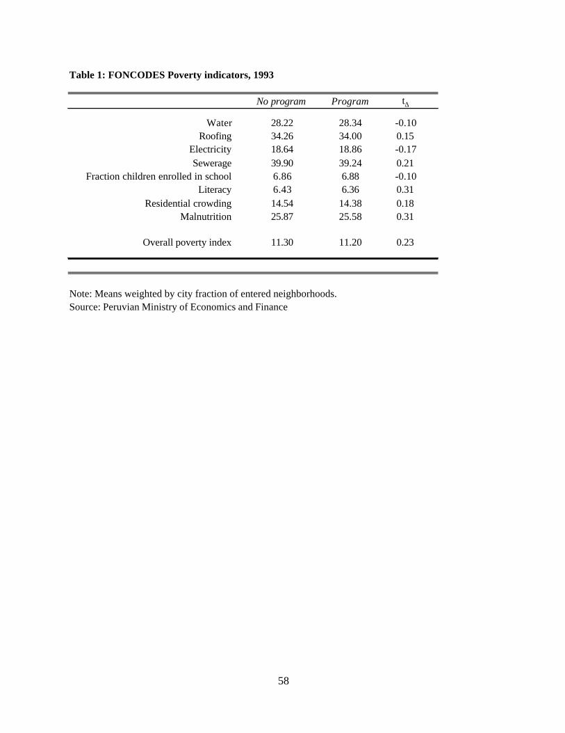
58

No program Program t∆

Water 28.22 28.34 -0.10Roofing 34.26 34.00 0.15

Electricity 18.64 18.86 -0.17Sewerage 39.90 39.24 0.21

Fraction children enrolled in school 6.86 6.88 -0.10Literacy 6.43 6.36 0.31

Residential crowding 14.54 14.38 0.18Malnutrition 25.87 25.58 0.31

Overall poverty index 11.30 11.20 0.23

Source: Peruvian Ministry of Economics and FinanceNote: Means weighted by city fraction of entered neighborhoods.

Table 1: FONCODES Poverty indicators, 1993

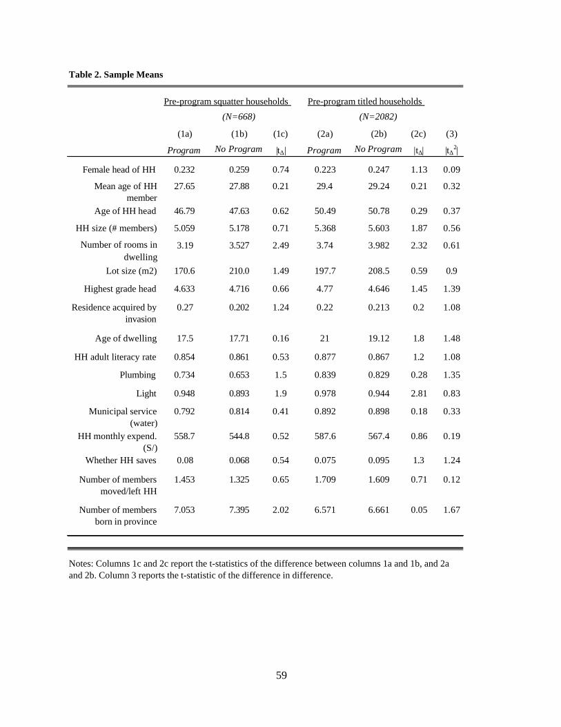
59

Table 2. Sample Means

(N=668) (N=2082)

(1a) (1b) (1c) (2a) (2b) (2c) (3)

Program No Program |t∆| Program No Program |t∆| |t∆2|

Female head of HH 0.232 0.259 0.74 0.223 0.247 1.13 0.09

27.65 27.88 0.21 29.4 29.24 0.21 0.32

Age of HH head 46.79 47.63 0.62 50.49 50.78 0.29 0.37

HH size (# members) 5.059 5.178 0.71 5.368 5.603 1.87 0.56

3.19 3.527 2.49 3.74 3.982 2.32 0.61

Lot size (m2) 170.6 210.0 1.49 197.7 208.5 0.59 0.9

Highest grade head 4.633 4.716 0.66 4.77 4.646 1.45 1.39

0.27 0.202 1.24 0.22 0.213 0.2 1.08

Age of dwelling 17.5 17.71 0.16 21 19.12 1.8 1.48

HH adult literacy rate 0.854 0.861 0.53 0.877 0.867 1.2 1.08

Plumbing 0.734 0.653 1.5 0.839 0.829 0.28 1.35

Light 0.948 0.893 1.9 0.978 0.944 2.81 0.83

0.792 0.814 0.41 0.892 0.898 0.18 0.33

558.7 544.8 0.52 587.6 567.4 0.86 0.19

Whether HH saves 0.08 0.068 0.54 0.075 0.095 1.3 1.24

1.453 1.325 0.65 1.709 1.609 0.71 0.12

7.053 7.395 2.02 6.571 6.661 0.05 1.67

Pre-program squatter households Pre-program titled households

Mean age of HH member

Number of rooms in dwelling

Number of members born in province

Notes: Columns 1c and 2c report the t-statistics of the difference between columns 1a and 1b, and 2a and 2b. Column 3 reports the t-statistic of the difference in difference.

Residence acquired by invasion

Municipal service (water)

HH monthly expend. (S/)

Number of members moved/left HH

60

No Program Program Difference

(not yet entered) (entered)

Not squatter 0.586 0.657 0.071(N=1921) (0.012) (0.019) (0.023)

Squatter 0.000 0.674 0.674 0.603**(N=559) (0.000) (0.029) (0.037) (0.045)

No Program Program Difference(not yet entered) (entered)

Not squatter 0.181 0.093 -0.088(N=1921) (0.011) (0.013) (0.017)

Squatter 0.433 0.157 -0.276 -0.188**(N=559) (0.023) (0.019) (0.030) (0.035)

Table 3c: Do you consider dwelling currently very secure from eviction/invasion?

No Program Program Difference

(not yet entered) (entered)

Not squatter 0.333 0.377 0.044(N=1921) (0.012) (0.020) (0.024)

Squatter 0.148 0.379 0.232 0.188**(N=559) (0.026) (0.030) (0.040) (0.046)

* Significant at the 0.05% level. ** Significant at the 0.01% level.Notes: Standard errors in parentheses. Only eligible HHs (according to residential tenure) included. Change in tenure security in Table 3a comes from survey question: "Did the last property document you obtained affect the security of your residence?" asked only of households with property documents. Data in Table 3b and 3c based on responses to survey question, "How secure do you consider your property?" Respondents could report: (1) Very secure, I do not believe that it will be taken; (2) Secure; (3) Not so secure, I believe that in any moment it could be taken; (4) Not at all secure, I believe that it is very probable that at some moment it will be taken. Table 3b classifies households as "at risk" if they answer (3) or (4).

Difference-in-difference

Difference-in-difference

Tables 3a-3c: Evidence of Program Effect on Perceived Tenure Security

Table 3a: Large change in tenure security with last title

Table 3b: Do you consider dwelling currently at risk of eviction/invasion?

Difference-in-difference

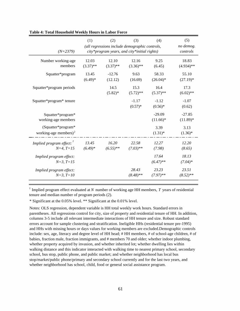
61

Table 4: Total Household Weekly Hours in Labor Force

(5)

(N=2379)no demog. controls

12.03 12.10 12.16 9.25 18.83(3.37)** (3.37)** (3.36)** (6.45) (4.934)**

13.45 -12.76 9.63 58.33 55.10(6.49)* (12.12) (16.69) (26.04)* (27.19)*

14.5 15.3 16.4 17.3(5.82)* (5.72)** (5.37)** (6.02)**

-1.17 -1.12 -1.07(0.57)* (0.56)* (0.62)

-29.09 -27.85(11.66)* (11.89)*

3.39 3.13(1.31)* (1.36)*

13.45 16.20 22.58 12.27 12.20(6.49)* (6.55)** (7.03)** (7.98) (8.65)

17.64 18.13(6.47)** (7.04)*

28.43 23.23 23.51(8.48)** (7.97)** (8.52)**

Implied program effect: †

N=4, T=15

Implied program effect: N=3, T=15

Implied program effect: N=3, T=10

Notes: OLS regression, dependent variable is HH total weekly work hours. Standard errors in parentheses. All regressions control for city, size of property and residential tenure of HH. In addition, columns 3-5 include all relevant intermediate interactions of HH tenure and size. Robust standard errors account for sample clustering and stratification. Ineligible HHs (residential tenure pre-1995) and HHs with missing hours or days values for working members are excluded.Demographic controls include: sex, age, literacy and degree level of HH head; # HH members, # of school-age children, # of babies, fraction male, fraction immigrants, and # members 70 and older; whether indoor plumbing, whether property acquired by invasion, and whether inherited lot; whether dwelling lies within walking distance and this indicator interacted with walking time to nearest primary school, secondary school, bus stop, public phone, and public market; and whether neighborhood has local bus stop/market/public phone/primary and secondary school currently and for the last two years, and whether neighborhood has school, child, food or general social assistance program.

* Significant at the 0.05% level. ** Significant at the 0.01% level.

(1) (2) (3) (4)(all regressions include demographic controls,

city*program years, and city*initial rights)

Number working-age members

Squatter*program

† Implied program effect evaluated at N number of working age HH members, T years of residential tenure and median number of program periods (2).

Squatter*program periods

Squatter*program* tenure

Squatter*program* working-age members

(Squatter*program* working-age members)2

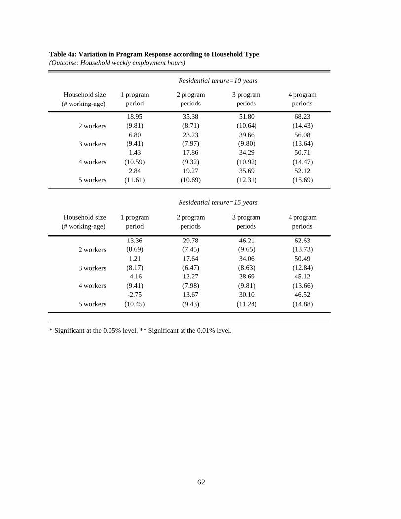
62

Household size (# working-age)

18.95 35.38 51.80 68.23 (9.81) (8.71) (10.64) (14.43)6.80 23.23 39.66 56.08

(9.41) (7.97) (9.80) (13.64)1.43 17.86 34.29 50.71

(10.59) (9.32) (10.92) (14.47)2.84 19.27 35.69 52.12

(11.61) (10.69) (12.31) (15.69)

Household size (# working-age)

1 program period

2 program periods

3 program periods

4 program periods

13.36 29.78 46.21 62.63 (8.69) (7.45) (9.65) (13.73)1.21 17.64 34.06 50.49

(8.17) (6.47) (8.63) (12.84)-4.16 12.27 28.69 45.12 (9.41) (7.98) (9.81) (13.66)-2.75 13.67 30.10 46.52

(10.45) (9.43) (11.24) (14.88)

* Significant at the 0.05% level. ** Significant at the 0.01% level.

Table 4a: Variation in Program Response according to Household Type (Outcome: Household weekly employment hours)

Residential tenure=10 years

1 program period

2 program periods

3 program periods

4 program periods

2 workers

3 workers

4 workers

5 workers

4 workers

5 workers

Residential tenure=15 years

2 workers

3 workers

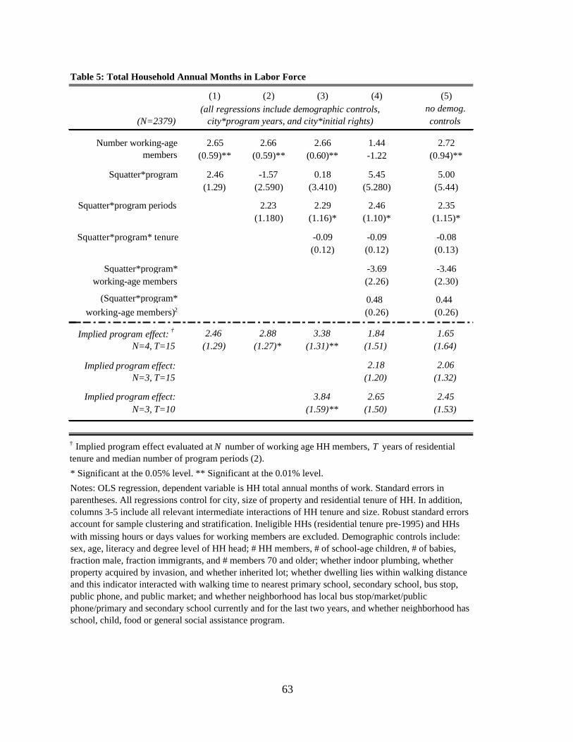
63

Table 5: Total Household Annual Months in Labor Force

(5)

(N=2379)no demog. controls

2.65 2.66 2.66 1.44 2.72(0.59)** (0.59)** (0.60)** -1.22 (0.94)**

2.46 -1.57 0.18 5.45 5.00(1.29) (2.590) (3.410) (5.280) (5.44)

2.23 2.29 2.46 2.35(1.180) (1.16)* (1.10)* (1.15)*

-0.09 -0.09 -0.08(0.12) (0.12) (0.13)

-3.69 -3.46(2.26) (2.30)

0.48 0.44(0.26) (0.26)

2.46 2.88 3.38 1.84 1.65(1.29) (1.27)* (1.31)** (1.51) (1.64)

2.18 2.06(1.20) (1.32)

3.84 2.65 2.45(1.59)** (1.50) (1.53)

(1) (2) (3) (4)(all regressions include demographic controls,

city*program years, and city*initial rights)

Number working-age members

Squatter*program

Squatter*program periods

Squatter*program* tenure

Squatter*program* working-age members

(Squatter*program* working-age members)2

Implied program effect: †

N=4, T=15

Implied program effect: N=3, T=15

Implied program effect: N=3, T=10

Notes: OLS regression, dependent variable is HH total annual months of work. Standard errors in parentheses. All regressions control for city, size of property and residential tenure of HH. In addition, columns 3-5 include all relevant intermediate interactions of HH tenure and size. Robust standard errors account for sample clustering and stratification. Ineligible HHs (residential tenure pre-1995) and HHs with missing hours or days values for working members are excluded. Demographic controls include: sex, age, literacy and degree level of HH head; # HH members, # of school-age children, # of babies, fraction male, fraction immigrants, and # members 70 and older; whether indoor plumbing, whether property acquired by invasion, and whether inherited lot; whether dwelling lies within walking distance and this indicator interacted with walking time to nearest primary school, secondary school, bus stop, public phone, and public market; and whether neighborhood has local bus stop/market/public phone/primary and secondary school currently and for the last two years, and whether neighborhood has school, child, food or general social assistance program.

† Implied program effect evaluated at N number of working age HH members, T years of residential tenure and median number of program periods (2).

* Significant at the 0.05% level. ** Significant at the 0.01% level.

64

Table 6: Fraction of Household Members in Labor Force

(5)

(N=2379)no demog. controls

-0.042 -0.042 -0.042 -0.095 -0.08(0.011)** (0.011)** (0.011)** (0.018)** (0.017)*

0.063 -0.033 -0.019 0.207 0.198(0.028)* (0.050) (0.065) (0.156) (0.173)

0.053 0.056 0.058 0.058(0.021)* (0.021)** (0.020)** (0.022)**

-0.001 -0.000 -0.000(0.003) (0.003) (0.003)

-0.112 -0.107(0.060) (0.065)

0.011 0.010(0.005)* (0.006)

0.063 0.073 0.080 0.046 0.045(0.028)* (0.027)* (0.027)** (0.029) (0.031)

0.081 0.082(0.034)* (0.038)*

0.080 0.083 0.082(0.035)** (0.038)* (0.041)*

Implied program effect: N=3, T=15

Implied program effect: N=3, T=10

Notes: OLS regression, dependent variable is percentage of working-age HH members who are either employed or searching for a job. Standard errors in parentheses. All regressions control for city, size of property and residential tenure of HH. In addition, columns 3-5 include all relevant intermediate interactions of HH tenure and size. Robust standard errors account for sample clustering and stratification. Ineligible HHs (residential tenure pre-1995) and HHs with missing hours or days values for working members are excluded. Demographic controls include: sex, age, literacy and degree level of HH head; # HH members, # of school-age children, # of babies, fraction male, fraction immigrants, and # members 70 and older; whether indoor plumbing, whether property acquired by invasion, and whether inherited lot; whether dwelling lies within walking distance and this indicator interacted with walking time to nearest primary school, secondary school, bus stop, public phone, and public market; and whether neighborhood has local bus stop/market/public phone/primary and secondary school currently and for last two years, and whether neighborhood has school, child, food or social assistance program.

† Implied program effect evaluated at N number of working age HH members, T years of residential tenure and median number of program periods (2).* Significant at the 0.05% level. ** Significant at the 0.01% level.

Squatter*program* tenure

Squatter*program* working-age members

(Squatter*program* working-age members)2

Implied program effect: †

N=4, T=15

(all regressions include demographic controls, city*program years, and city*initial rights)

Number working-age members

Squatter*program

Squatter*program periods

(1) (2) (3) (4)

65

Table 7: Gender Distribution of Household Weekly Hours

(1) (2) (3) (4) (5) (6)

(N=2379)Total Hours Men Women

Total Hours Men Women

6.10 0.53 2.76 6.40 0.78 3.68(3.44) (2.20) (1.93) (6.13) (4.01) (3.03)

17.78 26.64 16.45 26.59(5.79)** (4.01)** (5.78)** (4.05)**

12.69 21.25 11.12 19.86(4.74)** (2.74)** (4.69)* (2.69)**

12.92 10.35 2.69 80.93 10.02 66.39(6.17)* (4.26)* (4.12) (24.74)** (17.51) (15.41)**

-0.98 0.07 -0.93(0.54) (0.38) (0.35)**

-27.53 -0.91 -25.44(11.50)* (8.46) (7.31)**

3.24 0.16 2.96(1.27)* (0.96) (0.80)**

Mean Program Effect 12.92 10.35 2.69 8.06 9.98 -1.95SE (6.17)* (4.26)** (4.12) (7.88) (5.38) (5.35)

* Significant at the 0.05% level. ** Significant at the 0.01% level.

Squatter*program* tenure

Squatter*program* working-age members

(Squatter*program* working-age members)2

Number working-age members

Number adult men

Number adult women

Squatter*program

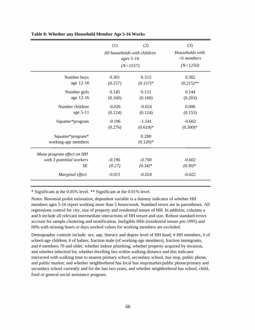
66

Table 8: Whether any Household Member Age 5-16 Works

Households with <6 members

(N=1250)

0.301 0.315 0.582(0.157) (0.157)* (0.215)**

0.145 0.151 0.144(0.160) (0.160) (0.203)

-0.026 -0.024 0.006(0.124) (0.124) (0.155)

Squatter*program -0.196 -1.541 -0.602(0.276) (0.619)* (0.300)*

0.280(0.120)*

-0.196 -0.700 -0.602SE (0.27) (0.34)* (0.30)*

Marginal effect -0.015 -0.024 -0.022

* Significant at the 0.05% level. ** Significant at the 0.01% level.

(1) (2) (3)

All households with children ages 5-16

(N=1557)

Number boys age 12-16

Number girls age 12-16

Demographic controls include: sex, age, literacy and degree level of HH head; # HH members, # of school-age children, # of babies, fraction male (of working-age members), fraction immigrants, and # members 70 and older; whether indoor plumbing, whether property acquired by invasion, and whether inherited lot; whether dwelling lies within walking distance and this indicator interacted with walking time to nearest primary school, secondary school, bus stop, public phone, and public market; and whether neighborhood has local bus stop/market/public phone/primary and secondary school currently and for the last two years, and whether neighborhood has school, child, food or general social assistance program.

Number children age 5-11

Squatter*program* working-age members

Mean program effect on HH with 3 potential workers

Notes: Binomial probit estimation, dependent variable is a dummy indicator of whether HH members ages 5-16 report working more than 5 hours/week. Standard errors are in parentheses. All regressions control for city, size of property and residential tenure of HH. In addition, columns a and b include all relevant intermediate interactions of HH tenure and size. Robust standard errors account for sample clustering and stratification. Ineligible HHs (residential tenure pre-1995) and HHs with missing hours or days worked values for working members are excluded.

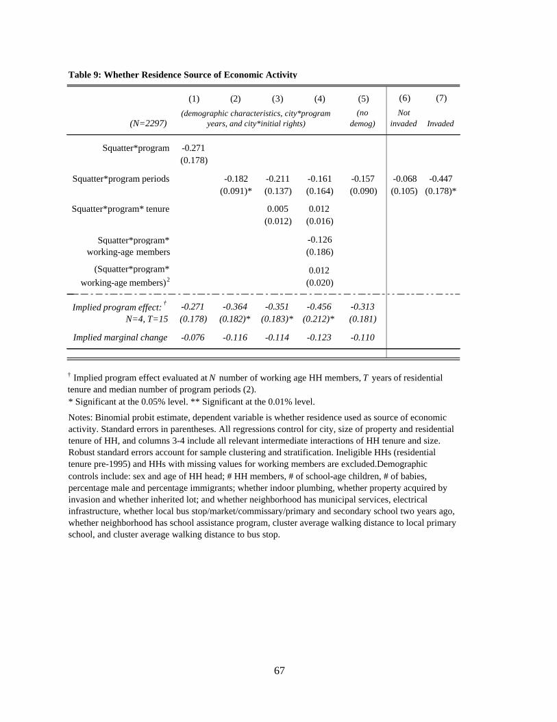
67

Table 9: Whether Residence Source of Economic Activity

(6) (7)

(N=2297)(no

demog)Not

invaded Invaded

-0.271(0.178)

-0.182 -0.211 -0.161 -0.157 -0.068 -0.447(0.091)* (0.137) (0.164) (0.090) (0.105) (0.178)*

0.005 0.012(0.012) (0.016)

-0.126(0.186)

0.012(0.020)

-0.271 -0.364 -0.351 -0.456 -0.313(0.178) (0.182)* (0.183)* (0.212)* (0.181)

Implied marginal change -0.076 -0.116 -0.114 -0.123 -0.110

(4)

* Significant at the 0.05% level. ** Significant at the 0.01% level.

Squatter*program periods

(1) (2) (3)

† Implied program effect evaluated at N number of working age HH members, T years of residential tenure and median number of program periods (2).

Notes: Binomial probit estimate, dependent variable is whether residence used as source of economic activity. Standard errors in parentheses. All regressions control for city, size of property and residential tenure of HH, and columns 3-4 include all relevant intermediate interactions of HH tenure and size. Robust standard errors account for sample clustering and stratification. Ineligible HHs (residential tenure pre-1995) and HHs with missing values for working members are excluded.Demographic controls include: sex and age of HH head; # HH members, # of school-age children, # of babies, percentage male and percentage immigrants; whether indoor plumbing, whether property acquired by invasion and whether inherited lot; and whether neighborhood has municipal services, electrical infrastructure, whether local bus stop/market/commissary/primary and secondary school two years ago, whether neighborhood has school assistance program, cluster average walking distance to local primary school, and cluster average walking distance to bus stop.

(5)

Squatter*program* tenure

Squatter*program* working-age members

(Squatter*program* working-age members)2

Implied program effect: †

N=4, T=15

(demographic characteristics, city*program years, and city*initial rights)

Squatter*program

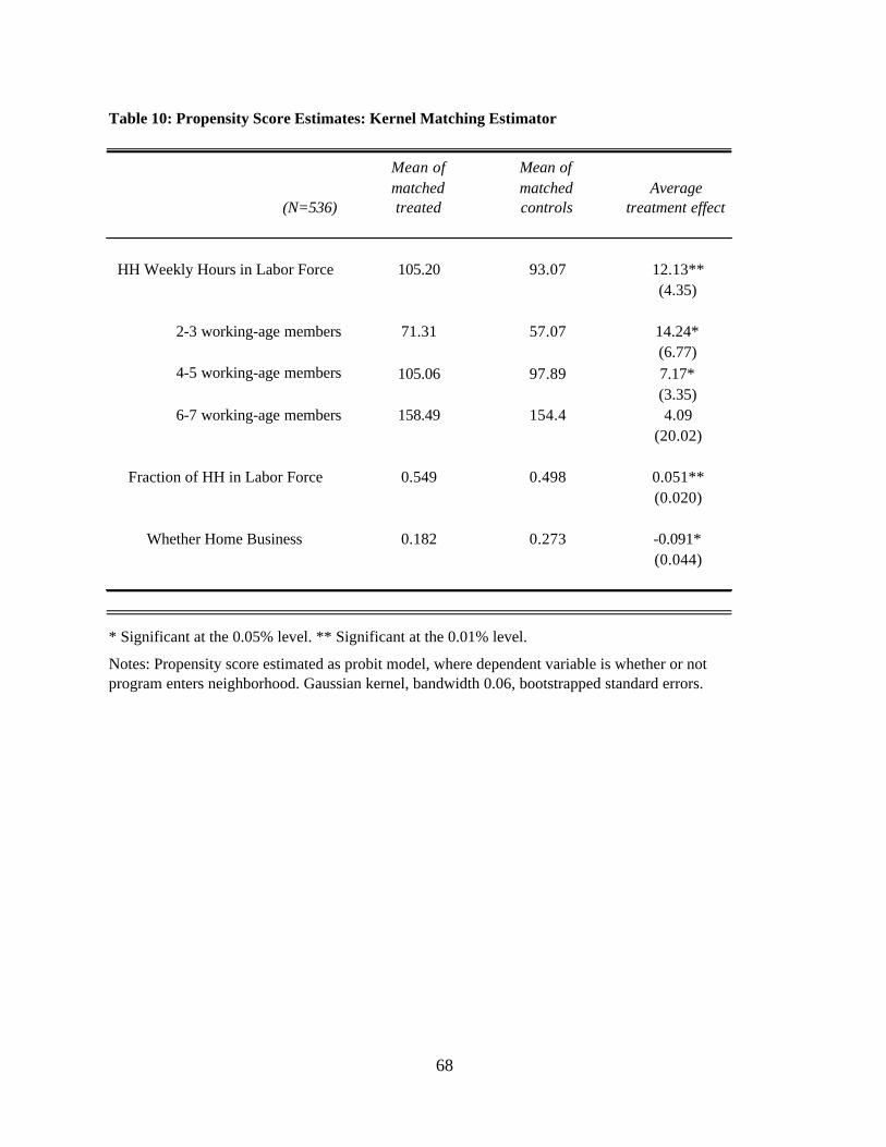
68

Table 10: Propensity Score Estimates: Kernel Matching Estimator

(N=536)

105.20 93.07 12.13**(4.35)

2-3 working-age members 71.31 57.07 14.24*(6.77)

4-5 working-age members 105.06 97.89 7.17*(3.35)

6-7 working-age members 158.49 154.4 4.09(20.02)

0.549 0.498 0.051**(0.020)

0.182 0.273 -0.091*(0.044)

* Significant at the 0.05% level. ** Significant at the 0.01% level.

Fraction of HH in Labor Force

Whether Home Business

Notes: Propensity score estimated as probit model, where dependent variable is whether or not program enters neighborhood. Gaussian kernel, bandwidth 0.06, bootstrapped standard errors.

Mean of matched treated

Mean of matched controls

Average treatment effect

HH Weekly Hours in Labor Force

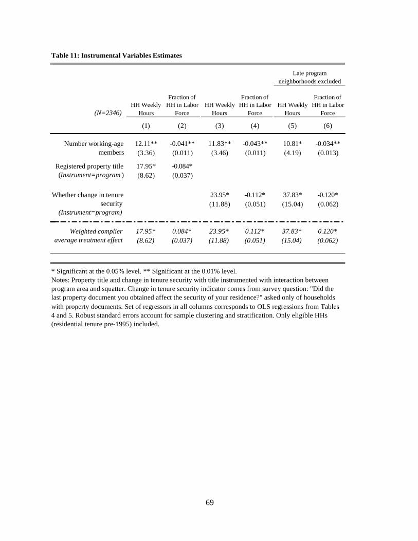
69

Table 11: Instrumental Variables Estimates

(N=2346)

(1) (2) (3) (4) (5) (6)

12.11** -0.041** 11.83** -0.043** 10.81* -0.034**(3.36) (0.011) (3.46) (0.011) (4.19) (0.013)

17.95* -0.084*(8.62) (0.037)

23.95* -0.112* 37.83* -0.120*(11.88) (0.051) (15.04) (0.062)

17.95* 0.084* 23.95* 0.112* 37.83* 0.120*(8.62) (0.037) (11.88) (0.051) (15.04) (0.062)

* Significant at the 0.05% level. ** Significant at the 0.01% level.

Weighted complier average treatment effect

Notes: Property title and change in tenure security with title instrumented with interaction between program area and squatter. Change in tenure security indicator comes from survey question: "Did the last property document you obtained affect the security of your residence?" asked only of households with property documents. Set of regressors in all columns corresponds to OLS regressions from Tables 4 and 5. Robust standard errors account for sample clustering and stratification. Only eligible HHs (residential tenure pre-1995) included.

Number working-age members

Registered property title (Instrument=program )

Whether change in tenure security

(Instrument=program)

Late program neighborhoods excluded

HH Weekly Hours

Fraction of HH in Labor

ForceHH Weekly

Hours

Fraction of HH in Labor

ForceHH Weekly

Hours

Fraction of HH in Labor

Force

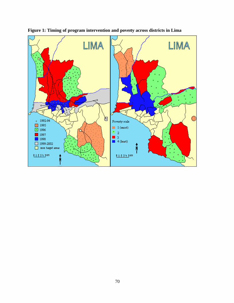
70

Figure 1: Timing of program intervention and poverty across districts in Lima

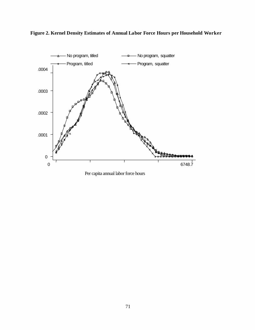
71

Figure 2. Kernel Density Estimates of Annual Labor Force Hours per Household Worker

Per capita annual labor force hours

No program, titled No program, squatter

Program, titled Program, squatter

0 6748.7

0

.0001

.0002

.0003

.0004

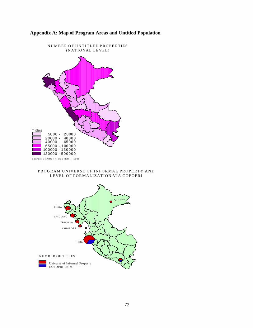
72

Appendix A: Map of Program Areas and Untitled Population

S o u r c e : E N A H O T R I M E S T E R I I , 1 9 9 8

T i t le s 5 0 0 0 - 2 0 0 0 0 2 0 0 0 0 - 4 0 0 0 0 4 0 0 0 0 - 6 5 0 0 0 6 5 0 0 0 - 1 0 0 0 0 0 1 0 0 0 0 0 - 1 3 0 0 0 0 1 3 0 0 0 0 - 5 0 0 0 0 0

N U M B E R O F U N T I T L E D P R O P E R T I E S ( N A T I O N A L L E V E L )

NUMBER OF TITLES Universe of Informal Property COFOPRI Titles

#

#

#

#

#

# #

# L I M A

P I U R A

H U A R A Z

I Q U I T O S

C H I C L A Y O

T R U J I L L O

C H I M B O T E

A R E Q U I P A

PROGRAM UNIVERSE OF INFORMAL PROPERTY AND

LEVEL OF FORMALIZATION VIA COFOPRI

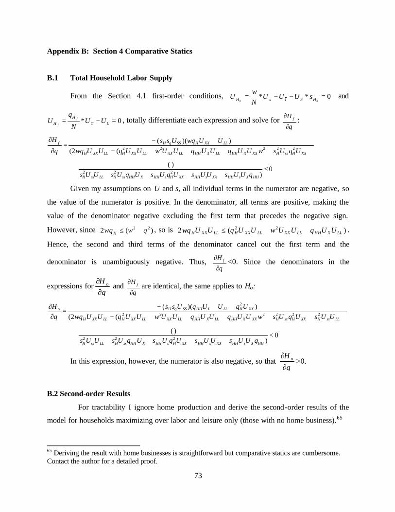
73

Appendix B: Section 4 Comparative Statics

B.1 Total Household Labor Supply

From the Section 4.1 first-order conditions, 0** =−−=oo HSlxH sUUU

Nw

U and

0* =−= LCH

H UUN

qU f

f, totally differentiate each expression and solve for

θ∂

∂ fH :

+++++−+−

=∂

∂

XXHssHXXXHHLLXHHLLXXLLXXHLLXXH

LLXXHSSHf

UqUswUUqUUqUUwUUqUUwqUUwqUssH

22222(2())(( θ

θ

0)

)(222 <

++++⋅

HHXsHHXXsHHXXHsHHXHHssHLLssH qUUsUUsUqUsUqUsUUs

Given my assumptions on U and s, all individual terms in the numerator are negative, so

the value of the numerator is positive. In the denominator, all terms are positive, making the

value of the denominator negative excluding the first term that precedes the negative sign.

However, since )(2 22 qwwqH +≤ , so is )(2 22LLXHHLLXXLLXXHLLXXH UUqUUwUUqUUwq ++≤ .

Hence, the second and third terms of the denominator cancel out the first term and the

denominator is unambiguously negative. Thus, θ∂

∂ fH <0. Since the denominators in the

expressions forθ∂

∂ oH and

θ∂

∂ fH are identical, the same applies to Ho:

++++++−++−

=∂

∂

LLssHXXHssHXXXHHLLXHHLLXXLLXXHLLXXH

XXHLLLHHSSHo

UUsUqUswUUqUUqUUwUUqUUwqUqUUqUssH

222222

2

(2())(( θ

θ

0)

)(222 <

++++⋅

HHXsHHXXsHHXXHsHHXHHssHLLssH qUUsUUsUqUsUqUsUUs

In this expression, however, the numerator is also negative, so that θ∂

∂ oH>0.

B.2 Second-order Results

For tractability I ignore home production and derive the second-order results of the

model for households maximizing over labor and leisure only (those with no home business).65

65 Deriving the result with home businesses is straightforward but comparative statics are cumbersome. Contact the author for a detailed proof.

74

The household’s optimization problem is written as:

)),,(,max,

τθLsl,xU(lx

s.t. XLHw =−∗ )(

)),,(,),(max,

τθLsNL

LHNw

U(lx

−⇒

Because of the assumptions ∞==0| XXU and ∞==0|LLU , the optimal solution will be

interior. The first-order condition for an interior optimum is:

01 =∗++∗−=

∂∂

sLlx UsUN

UNw

LU

Taking the total derivative I obtain the following expression for θ∂

∂L:

]1

)(2

22)[(

1

22

22

LLsLLLssLLsLXsXLXX

LsLssLsXs

sUUN

sUsUN

sUNw

UNw

UNw

sUssUsUN

sUNw

L

∗+∗+∗+∗∗+∗∗∗−∗∗−∗

∗−∗∗−∗∗−∗∗=

∂∂ θθθθ

θ

Because of the assumptions on ,, XLXs UU and LsU , the numerator is positive and the

denominator is negative. Therefore 0<∂∂θL

.

Continuing with the assumption of additive separability, the second-order results of the

model are derived by taking the second derivatives with respect to the implicit functions.

Consider the case of τ . The expression for τθ∂∂

∂ L2

is found by applying the chain rule to the above

expressions for θ∂

∂L and τ∂

∂L :

2

2

2

222

2

)(

)()(

Lf

ffLL

fLffL

Lf

L

∂∂

∂∂

∂∂∂

+∂∂

∂∂

+∂∂

∂∂∂

+∂∂

∂∂∂

−=

∂∂∂ θτθττθτθ

τθ

Assuming that all third derivatives of U and s are weakly positive (as in the case of

CARA or CRRA or quadratic utility functions), the numerator of the above expression is positive

and the denominator is negative, so that τθ∂∂

∂ L2

<0. An analogous proof follows for N.

75

B.3 Labor Supply of Children

Here I expand the model to incorporate differences in the household supply of adult and

child labor, and show that under the simplifying assumption that only adult leisure contributes to

home security, in households in which children are labor force participants, child labor hours will

fall with an increase in tenure security while adult labor hours rise. To see this, consider a

household with one child and one adult, where lA and lC are adult and child leisure, respectively,

and hA and hC are adult and child time endowments. As before, household utility is a function of

individuals’ leisure, per capita consumption, and home security. The same functional form

assumptions as before apply to s(.) and U(.). The only difference here is that only adult leisure

enters the security function, and 0=CAllU . The household’s maximization problem is then:

)),,(,max,,

τθACAxll

ls,l,lxU(CA

s.t. Xlhwlhw CCCAAA =−∗+−∗ )()(

The first order conditions for a utility maximum are:

02

=∗++∗−=∂∂

sLlxA

A

UsUUw

lU

A

02

=+∗−=∂∂

ClxC

C

UUw

lU

If U is additively separable in its arguments, by taking the total derivatives of the first

order conditions, we can obtain the following expressions for θ∂

∂ Cl and θ∂

∂ Al:

0][

)(2222222 >

+++++−+−

=∂∂

LLsllLssllllllXXALLsXXCLssXXCllXXC

XXCALSSSLC

sUUsUUUUUwsUUwsUUwUUwUwwsUUssl

CCCCAACCAA

θθ

θ

0][

))((2222222

2

<+++++−

++=

∂∂

LLsllLssllllllXXALLsXXCLssXXCllXXC

llXXCLSSSLA

sUUsUUUUUwsUUwsUUwUUw

UUwsUUssl

CCCCAACCAA

CCθθ

θ

Child leisure will rise with an increase in formal property rights, and adult leisure will fall.

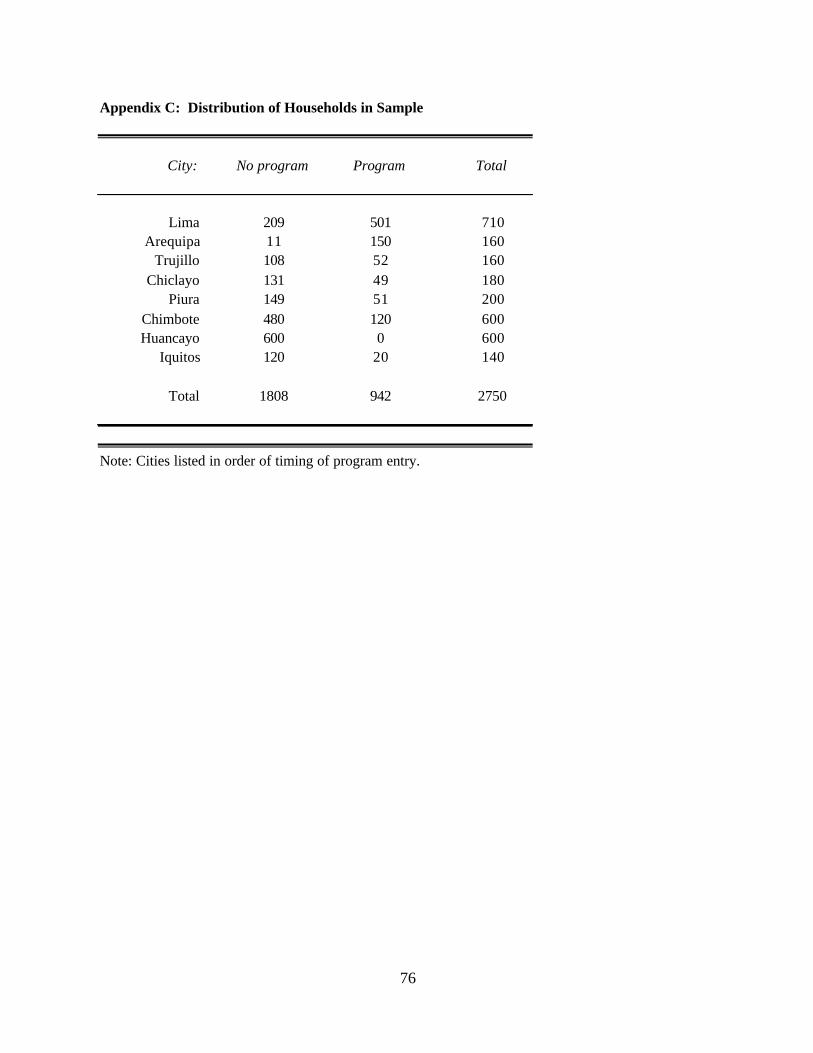
76

City: No program Program Total

Lima 209 501 710Arequipa 11 150 160

Trujillo 108 52 160Chiclayo 131 49 180

Piura 149 51 200Chimbote 480 120 600Huancayo 600 0 600

Iquitos 120 20 140

Total 1808 942 2750

Note: Cities listed in order of timing of program entry.

Appendix C: Distribution of Households in Sample

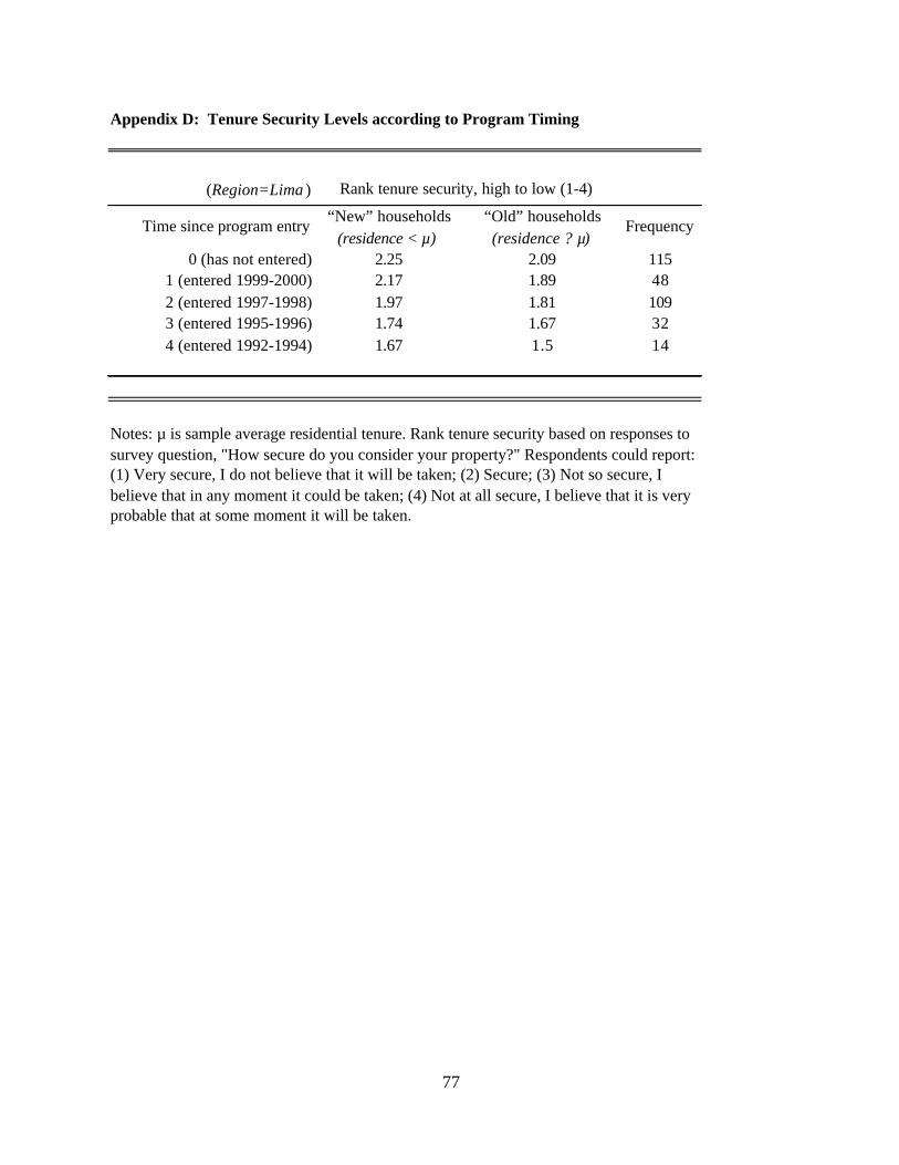
77

Appendix D: Tenure Security Levels according to Program Timing

(Region=Lima )

“New” households “Old” households(residence < µ) (residence ? µ)

0 (has not entered) 2.25 2.09 1151 (entered 1999-2000) 2.17 1.89 482 (entered 1997-1998) 1.97 1.81 1093 (entered 1995-1996) 1.74 1.67 324 (entered 1992-1994) 1.67 1.5 14

Rank tenure security, high to low (1-4)

Time since program entry Frequency

Notes: µ is sample average residential tenure. Rank tenure security based on responses to survey question, "How secure do you consider your property?" Respondents could report: (1) Very secure, I do not believe that it will be taken; (2) Secure; (3) Not so secure, I believe that in any moment it could be taken; (4) Not at all secure, I believe that it is very probable that at some moment it will be taken.

78

Appendix E: Test of Linearity in Program Periods

(1) (2) (3)

(N=2394) Weekly hours LFP Home Business

74.63 0.267 -0.022(25.49)** (0.153) (0.061)

92.45 0.335 -0.059(25.78)** (0.161)* (0.063)

107.26 0.371 -0.099(27.02)** (0.157)* (0.108)

123.55 0.452 -0.318(30.40)** (0.160)** (0.075)**

-1.12 -0.001(0.55)* (0.003)

-29.18 -0.113(11.72)* (0.061)

3.4 0.011(1.31)* (0.005)*

F(2, 258) = 0.12 0.13 1.15Prob > F = 0.888 0.883 0.319

* Significant at the 0.05% level. ** Significant at the 0.01% level.

Notes: Sets of regressors correspond to Tables 4, 5 and 9. Robust standard errors account for sample clustering and stratification. Only eligible HHs (residential tenure pre-1995) included.

Squatter*program* tenure

Squatter*program* working-age members

(Squatter*program* working-age members)2

Adjusted Wald Test: (PP4-PP3)=(PP3-PP2)=(PP2-PP1)

Squatter*program period 1

Squatter*program period 2

Squatter*program period 3

Squatter*program period 4

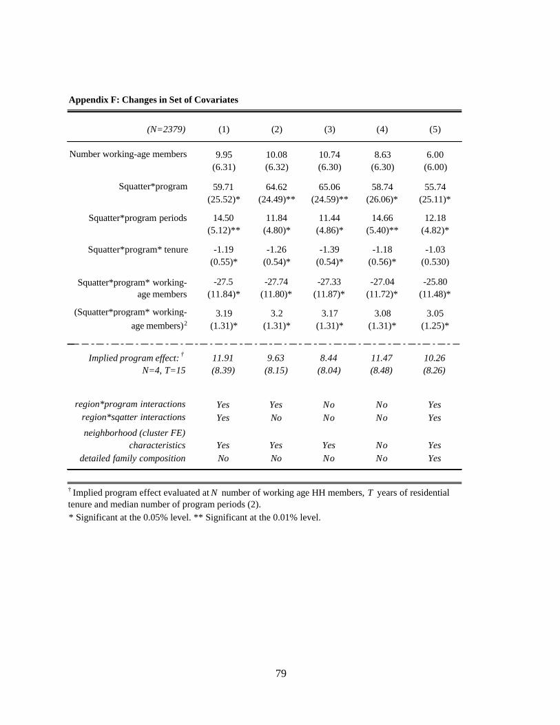
79

Appendix F: Changes in Set of Covariates

(N=2379)

9.95 10.08 10.74 8.63 6.00(6.31) (6.32) (6.30) (6.30) (6.00)

59.71 64.62 65.06 58.74 55.74(25.52)* (24.49)** (24.59)** (26.06)* (25.11)*

14.50 11.84 11.44 14.66 12.18(5.12)** (4.80)* (4.86)* (5.40)** (4.82)*

-1.19 -1.26 -1.39 -1.18 -1.03(0.55)* (0.54)* (0.54)* (0.56)* (0.530)

-27.5 -27.74 -27.33 -27.04 -25.80(11.84)* (11.80)* (11.87)* (11.72)* (11.48)*

3.19 3.2 3.17 3.08 3.05(1.31)* (1.31)* (1.31)* (1.31)* (1.25)*

11.91 9.63 8.44 11.47 10.26(8.39) (8.15) (8.04) (8.48) (8.26)

region*program interactions Yes Yes No No Yesregion*sqatter interactions Yes No No No Yes

neighborhood (cluster FE) characteristics Yes Yes Yes No Yes

detailed family composition No No No No Yes

* Significant at the 0.05% level. ** Significant at the 0.01% level.

† Implied program effect evaluated at N number of working age HH members, T years of residential tenure and median number of program periods (2).

Squatter*program* tenure

Squatter*program* working-age members

(Squatter*program* working-age members)2

Implied program effect: †

N=4, T=15

(5)

Number working-age members

Squatter*program

Squatter*program periods

(1) (2) (3) (4)