environment performance_index2008.pdf
TRANSCRIPT

1
2008 ENVIRONMENTAL PERFORMANCE INDEX Yale Center for Environmental Law & Policy Yale University Center for International Earth Science Information Network (CIESIN) Columbia University In collaboration with
World Economic Forum Geneva, Switzerland Joint Research Centre of the European Commission Ispra, Italy

2
ACKNOWLEDGEMENTS AUTHORS Yale Center for Environmental Law & Policy, Yale University http://www.yale.edu/envirocenter Daniel C. Esty Christine Kim Tanja Srebotnjak Director Program Director Statistician
Center for International Earth Science Information Network, Columbia University http://ciesin.columbia.edu Marc A. Levy Alex de Sherbinin Valentina Mara Deputy Director Senior Research Associate Research Associate COLLABORATORS World Economic Forum http://www.weforum.org Fiona Paua Senior Director, Head of Strategic Insight Teams Joint Research Centre (JRC), European Commission http://www.jrc.ec.europa.eu/
Andrea Saltelli Unit Head Michaela Saisana Researcher DESIGN AND DATA VISUALIZATION Tamara Maletic http://linkedbyair.net Linked By Air Dan Michelson Linked By Air The full report and data can be found online at:
http://epi.yale.edu © Yale Center for Environmental Law & Policy

3
LEAD SCIENTIFIC EXPERTS Geneviève Carr UNEP GEMS/Water Programme
Aaron Cohen Health Effects Institute
Jay Emerson Yale University
Peter Gleick Pacific Institute
Lloyd Irland Yale University
Kewin Kamelarczyk Food and Agriculture Organization
Jonathan Pershing World Resources Institute
Carmen Revenga The Nature Conservancy
Sara J. Scherr Eco-Agriculture Partners
Jackie Alder University of British Columbia
OTHER EXPERT CONTRIBUTORS John Aardenne Joint Research Centre, EC Kym Anderson University of Adelaide Michelle Bell Yale University
Tim Boucher The Nature Conservancy Amy Cassara World Resource Institutes Tom Damassa World Resources Institute Charlotte de Fraiture International Water Management Institute Kailash Govil Food and Agriculture Organization Brian Hill Pesticide Action Network Peter Holmgren Forestry and Agricultural Organization Jon Hoekstra The Nature Conservancy Malanding Jaiteh CIESIN
Michael Jennings The Nature Conservancy Carrie Rickwood UNEP GEMS/Water Ariela Summit Eco-Agriculture Partners Kirk Smith University of California, Berkeley Charles Vorosmarty University of New Hampshire Aaron Best Ecologic Crystal Davis World Resources Institute Andres Gomez Columbia University Tobias Hahn Yale University Claes Johansson United Nations Development Programme Hoseok Kim Korea Environment Institute Hak-Kyun Maeng Ministry of Environment of Korea
Denise Mauzerall Princeton University Sascha Müller-Kraenner The Nature Conservancy John O’Connor OconEco Kiran Pandey Global Environment Facility Tom Parris iSciences Papa Seck United Nations Development Programme Erik Thomsen DSS Lab YuLing Yang Taiwan Environmental Protection Agency Ruth Wilkie Erica Zell Battell Institute

2008 Environmental Performance Index
28-Jan-2008 4
RESEARCH STAFF – Yale Center for Environmental Law & PolicyMelissa Goodall Associate Director Jen Ace Research Assistant Sara Bushey Research Assistant Adrian Deveny Research Assistant Eva Gladek Research Assistant Allison Guy Research Assistant
Emily Hallet Research Assistant Lauren Hallett Research Assistant Yanjing Huang Research Assistant Brian Irving Research Assistant Claire Jahns Research Assistant Meng Ji Research Assitant
Namrata Kala Research Assistant Scott Laeser Research Assistant John Chung-En Liu Research Assistant Matthew Oden Research Assistant
Version 1.1 Suggested Citation Esty, Daniel C., M.A. Levy, C.H. Kim, A. de Sherbinin, T. Srebotnjak, and V. Mara. 2008. 2008 Environmental Performance Index. New Haven: Yale Center for Environmental Law and Policy. Disclaimers This 2008 Environmental Performance Index (EPI) tracks national environmental results on a quantitative basis, measuring proximity to an established set of policy targets using the best data available. Data constraints and limitations in methodology make this a work in progress. Further refinements will be undertaken over the next few years. Comments, suggestions, feedback, and referrals to better data sources are welcome at: http://epi.yale.edu or [email protected]. The word “country” is used loosely in this report to refer both to countries and other administrative or economic entities. Similarly the maps presented are for illustrative purposes and do not imply any political preference in cases where territory is under dispute. Acknowledgements The 2008 Environmental Performance Index (EPI) represents the result of extensive consultations with subject-area specialists, statisticians, and policymakers around the world. Since any attempt to measure environmental performance requires both an in-depth knowledge of each dimension as well as the relationships between dimensions and the application of sophisticated statistical techniques to each, we have drawn on the expertise of a network of individuals, including: Jackie Alder, Michelle Bell, Aaron Best, Tim Boucher, Geneviève Carr, Amy Cassara, Aaron Cohen, Tom Damassa, Crystal Davis, Ellen Douglas, Darlene Dube, Jay Emerson, Majid Ezzati, Charlotte de Fraiture, Stanley Jay Glidden, Andres Gomez, Tobias Hahn, Peter Holmgren, Jon Hoekstra, Peter Gleick, Kailash Govil, Lloyd Irland, Michael Jennings, Claes Johansson, Kewin Kamelarczyk, Daniel Kammen, Hoseok Kim, R. Andreas Kraemer, Hak-Kyun Maeng, Tamara Maletic, Vali Mara, Denise Mauzerall, Dan Michelson, Sascha Müller-Kraenner,

2008 Environmental Performance Index
28-Jan-2008 5
John O’Connor, Kiran Pandey, Tom Parris, Fiona Paua, Jonathan Pershing, Carmen Revenga, Carrie Rickwood, Kim Samuel-Johnson Sara J. Scherr, Papa Seck, Ariela Summit, Kirk Smith, Erik Thomsen, Charles Vorosmarty, Ruth Wilkie, YuLing Yang, and Erica Zell. We are particularly indebted to the staff and research assistants at the Yale Center for Environmental Law and Policy: Jen Ace, Sara Bushey, Adrian Deveny, Ysella Edyvean, Eva Gladek, Kaitlin Gregg, Allison Guy, Emily Hallet, Lauren Hallett, Yanjing Huang, Brian Irving, Claire Jahns, Meng Ji, Namrata Kala, Scott Laeser, and Matthew Oden. The 2008 EPI is built upon the work of a range of data providers, including our own prior data development work for the Pilot 2006 EPI and the 2005 Environmental Sustainability Index. The data are drawn primarily from international, academic, and research institutions with subject-area expertise, success in delivering operational data, and the capacity to produce policy-relevant interdisciplinary information tools. We are indebted to the data collection agencies listed in the Methodology Section, for providing the high-quality information necessary to move environmental decisionmaking toward more rigorous, quantitative foundations. We wish to acknowledge with gratitude the financial support of The Samuel Family Foundation, The Coca Cola Foundation, and the Betsy and Jesse Fink Foundation.
2008 Environmental Performance Index
28-Jan-2008 6
TABLE OF CONTENTS
ACKNOWLEDGEMENTS ....................................................................................2
TABLE OF CONTENTS .......................................................................................6
EXECUTIVE SUMMARY ......................................................................................8 Policy Conclusions ................................................................................................................... 8
1. THE NEED FOR ENVIRONMENTAL PERFORMANCE INDICATORS......11
2. THE EPI FRAMEWORK..............................................................................15 2.1. Indicator Selection and Targets................................................................................ 16 2.2. Data Gaps and Country Data Coverage................................................................... 17 2.3. Targets ........................................................................................................................ 21 2.4. Calculating the EPI..................................................................................................... 21 2.5. Data Aggregation and Weighting ............................................................................. 21
3: RESULTS AND ANALYSIS ........................................................................23 3.1. EPI Results by peer group ........................................................................................ 24
5. SENSITIVITY ANALYSIS............................................................................26 Summary.................................................................................................................................. 26
APPENDIX D: THE 2008 EPI, PILOT 2006 EPI, AND ENVIRONMENTAL SUSTAINABILITY INDEX ..................................................................................30
D.1. Comparison of the Pilot 2006 Environmental Performance Index and the 2008 Environmental Performance Index........................................................................................ 30 D.2. Comparison of the Environmental Sustainability Index and the Environmental Performance Index.................................................................................................................. 32
APPENDIX E: METHODOLOGY & MEASUREMENT CHALLENGES.........36 E.1. Country Selection Criteria......................................................................................... 36 E. 2. Target Selection ......................................................................................................... 37 E.3. Missing Data ............................................................................................................... 38 E. 4. Calculation of the EPI and Policy Category Sub-Indices....................................... 39 E.5. Cluster Analysis ......................................................................................................... 41
APPENDIX F: UNCERTAINTY AND SENSITIVITY ANALYSIS OF THE 2008 EPI ......................................................................................................................43
by Michaela Saisana and Andrea Saltelli.............................................................................. 43 F.1. How is the EPI associated to its subcomponents and policy categories?................ 43 Robustness of the EPI results to the methodological assumptions ................................. 46 Our approach........................................................................................................................... 47
APPENDIX E: INDICATOR METADATA ...........................................................61

2008 Environmental Performance Index
28-Jan-2008 7
FFOORRTTHHCCOOMMIINNGG MMAARRCCHH 22000088
• EXPANDED CHAPTER 3: RESULTS & ANALYSIS
• CHAPTER 4: POLICY CATEGORY DISCUSSION
• CHAPTER 6: CONCLUSIONS
• APPENDIX A: PDF OF POLICY CATEGORY TABLES
• APPENDIX B: PDF OF INDICATOR TABLES
• APPENDIX C: PDF OF COUNTRY PROFILES
• APPENDIX D: THE 2008 EPI, PILOT 2006 EPI, AND ENVIRONMENTAL SUSTAINABILITY INDEX

2008 Environmental Performance Index
28-Jan-2008 8
EXECUTIVE SUMMARY Fueled by advances in information technology, data-driven decisionmaking has transformed every corner of society, from business to biology. In the policy domain, quantitative performance metrics have reshaped decisionmaking processes in many arenas, including economics, health care, and education. The 2008 Environmental Performance Index (EPI) brings a similar data-driven, fact-based empirical approach to environmental protection and global sustainability. Policymakers in the environmental field have also begun to recognize the importance of incorporating analytically rigorous foundations into their decisionmaking. However, while policymakers are calling for increased intellectual rigor in environmental planning, large data gaps and a lack of time-series data still hamper efforts to track many environmental issues, spot emerging problems, assess policy options, and gauge effectiveness. The EPI seeks to being to fill these gaps and, more broadly, to draw attention to the value of accurate data and sound analysis as the basis for environmental policymaking. The EPI focuses on two overarching environmental objectives:
• reducing environmental stresses to human health; • promoting ecosystem vitality and sound natural resource management;.
These broad goals also reflect the policy priorities of environmental authorities around the world and the international community’s intent in adopting Goal 7 of the Millennium Development Goals (MDGs), to “ensure environmental sustainability.” The two overarching objectives are gauged using 25 performance indicators tracked in six well-established policy categories, which are then combined to create a final score. The 2008 EPI deploys a proximity-to-target methodology, which quantitatively tracks national performance on a core set of environmental policy goals for which every government can be – and should be – held accountable. By identifying specific targets and measuring the distance between the target and current national achievement, the EPI provides both an empirical foundation for policy analysis and a context for evaluating performance. Issue-by-issue and aggregate rankings facilitate cross-country comparisons both globally and within relevant peer groups such as geography or economy. It must be emphasized that the EPI’s real value lies not in the numerical rankings, but rather in careful analysis of the underlying data and performance metrics. The results are displayed in numerous ways: by issue, policy category, peer group, and country. This format facilitates identification of leaders and laggards, highlights best policy practices for each issue, and identifies priorities for action for each country. More generally, the EPI provides a powerful tool for steering environmental investments, refining policy choices, optimizing the impact of limited financial resources, and understanding the determinants of policy results. Policy Conclusions

2008 Environmental Performance Index
28-Jan-2008 9
• Environmental decisionmaking can and should be made more data-driven and rigorous. A more fact-based and empirical approach to policymaking promises systematically better results.
• Notwithstanding data gaps and methodological limitations, the EPI demonstrates that environmental results can be tracked quantitatively, facilitating more refined policy analysis.
• To address these gaps, policymakers should invest in collecting additional data and tracking a core set of indicators over time. They must also set clear policy targets and incorporate indicators and reporting into policy formation, and shift toward more analytically rigorous environmental protection efforts at the global, regional, national, state/provincial, local, and corporate scales.
• Environmental challenges come in several forms which vary with wealth and development. Some issues arise as a function of economic activity and its resource and pollution impacts, such that developed and industrializing countries face the most severe harms. Other threats derive from poverty or a lack of basic environmental amenities, such as access to safe drinking water and basic sanitation. The issues affect primarily developing nations.
• Wealth correlates highly with EPI scores and particularly with environmental
health results. But at every level of development, some countries achieve results that exceed their income-group peers. Statistical analysis suggests that in many cases good governance contributes to better environmental outcomes.
• The EPI uses the best available global datasets on environmental performance, but
the overall data quality and availability is alarmingly poor. The absence of broadly-collected and methodologically-consistent indicators for even basic concerns such as water quality – and the complete lack of time-series data for most countries – hampers efforts to shift pollution control and natural resource management onto more empirical foundations.
The 2008 EPI represents a “work in progress” intended not only to inform, but also to stimulate debate on defining the appropriate metrics and methodologies for evaluating environmental performance. As existing conceptual, methodological, and data challenges are overcome, better metrics will emerge – and a more refined EPI will be possible.

2008 Environmental Performance Index
28-Jan-2008 10
Table 1: EPI Scores (by rank) Rank Country EPI Rank Country EPI Rank Country EPI
1 Switzerland 95.5 51 South Korea 79.4 101 Laos 66.3 2 Sweden 93.1 52 Cyprus 79.2 102 Indonesia 66.2 3 Norway 93.1 53 Thailand 79.2 103 Côte d'Ivoire 65.2 4 Finland 91.4 54 Jamaica 79.1 104 Myanmar 65.1 5 Costa Rica 90.5 55 Netherlands 78.7 105 China 65.1 6 Austria 89.4 56 Bulgaria 78.5 106 Uzbekistan 65.0 7 New Zealand 88.9 57 Belgium 78.4 107 Kazakhstan 65.0 8 Latvia 88.8 58 Mauritius 78.1 108 Guyana 64.8 9 Colombia 88.3 59 Tunisia 78.1 109 Papua New Guinea 64.8 10 France 87.8 60 Peru 78.1 110 Bolivia 64.7 11 Iceland 87.6 61 Philippines 77.9 111 Kuwait 64.5 12 Canada 86.6 62 Armenia 77.8 112 United Arab Emirates 64.0 13 Germany 86.3 63 Paraguay 77.7 113 Tanzania 63.9 14 United Kingdom 86.3 64 Gabon 77.3 114 Cameroon 63.8 15 Slovenia 86.3 65 El Salvador 77.2 115 Senegal 62.8 16 Lithuania 86.2 66 Algeria 77.0 116 Togo 62.3 17 Slovakia 86.0 67 Iran 76.9 117 Uganda 61.6 18 Portugal 85.8 68 Czech Rep. 76.8 118 Swaziland 61.3 19 Estonia 85.2 69 Guatemala 76.7 119 Haiti 60.7 20 Croatia 84.6 70 Jordan 76.5 120 India 60.3 21 Japan 84.5 71 Egypt 76.3 121 Malawi 59.9 22 Ecuador 84.4 72 Turkey 75.9 122 Eritrea 59.4 23 Hungary 84.2 73 Honduras 75.4 123 Ethiopia 58.8 24 Italy 84.2 74 Macedonia 75.1 124 Pakistan 58.7 25 Denmark 84.0 75 Ukraine 74.1 125 Bangladesh 58.0 26 Malaysia 84.0 76 Viet Nam 73.9 126 Nigeria 56.2 27 Albania 84.0 77 Nicaragua 73.4 127 Benin 56.1 28 Russia 83.9 78 Saudi Arabia 72.8 128 Central African Rep. 56.0 29 Chile 83.4 79 Tajikistan 72.3 129 Sudan 55.5 30 Spain 83.1 80 Azerbaijan 72.2 130 Zambia 55.1 31 Luxembourg 83.1 81 Nepal 72.1 131 Rwanda 54.9 32 Panama 83.1 82 Morocco 72.1 132 Burundi 54.7 33 Dominican Rep. 83.0 83 Romania 71.9 133 Madagascar 54.6 34 Ireland 82.7 84 Belize 71.7 134 Mozambique 53.9 35 Brazil 82.7 85 Turkmenistan 71.3 135 Iraq 53.9 36 Uruguay 82.3 86 Ghana 70.8 136 Cambodia 53.8 37 Georgia 82.2 87 Moldova 70.7 137 Solomon Islands 52.3 38 Argentina 81.8 88 Namibia 70.6 138 Guinea 51.3 39 United States 81.0 89 Trinidad & Tobago 70.4 139 Djibouti 50.5 40 Taiwan 80.8 90 Lebanon 70.3 140 Guinea-Bissau 49.7 41 Cuba 80.7 91 Oman 70.3 141 Yemen 49.7 42 Poland 80.5 92 Fiji 69.7 142 Dem. Rep. Congo 47.3 43 Belarus 80.5 93 Congo 69.7 143 Chad 45.9 44 Greece 80.2 94 Kyrgyzstan 69.6 144 Burkina Faso 44.3 45 Venezuela 80.0 95 Zimbabwe 69.3 145 Mali 44.3 46 Australia 79.8 96 Kenya 69.0 146 Mauritania 44.2 47 Mexico 79.8 97 South Africa 69.0 147 Sierra Leone 40.0 48 Bosnia and
H i79.7 98 Botswana 68.7 148 Angola 39.5
49 Israel 79.6 99 Syria 68.2 149 Niger 39.1

2008 Environmental Performance Index
28-Jan-2008 11
1. THE NEED FOR ENVIRONMENTAL PERFORMANCE INDICATORS Environmental policymaking is difficult to do under the best of circumstances. Decisionmakers must address a wide range of pollution control and natural resource management challenges in the face of incomplete or conflicting data, causal complexity, divergent values and preferences, and myriad uncertainties. Without sufficient facts and careful analysis, each step of the process becomes more difficult—problems are harder to see, trends may not be understood, policy goals become more difficult to set, regulatory efforts may be misdirected, investments in environmental protection may be wasted, and optimum environmental performance will not be achieved. Shifting environmental policymaking onto firmer analytic foundations, based on carefully constructed data and indicators, therefore emerges as a matter of considerable urgency. The commitment to empirical data is just a first step. Identifying an appropriate set of metrics is equally important. Some past performance measurement initiatives have been too broad to be of great value.1 In covering sustainable development or sustainability in a “triple bottom line” fashion that combined environmental, social, and economic factors, as well as underlying endowments, accumulated harms, current policy efforts, and the prospect for changing future trajectories, these efforts lost coherence and therefore their policy relevance. Other efforts have been too narrow to cover the full spectrum of environmental challenges. In addressing only a subset of issues that policymakers and members of the scientific community identify as fundamental to meeting society’s environmental challenges.2 These indices have limited value. Our focus is on environmental sustainability and the current policy performance of individual nations. We have collected data on a broad-gauge list of core pollution and natural resource management challenges as identified by policy and scientific experts. While there is no “correct” answer to the proper scope of an environmental index, we believe our set of 25 indicators offers a comprehensive yet focused perspective on society’s environmental challenges. The EPI builds on a set of environmental indicators that can be addressed by current policymakers around the globe. Thus, building on the methodology established in the Pilot 2006 Environmental Performance Index (EPI), in addition to feedback from government and policy experts around the world, and the advice of dozens of scientific experts, the 2008 EPI centers on current national environmental performance. It tracks actual results (almost exclusively output measures) related to a core set of environmental issues that governments around the world have
1;See, for example, Esty, D.C., M. Levy, T. Srebotnjak and A. de Sherbinin. 2005. The 2005 Environmental Sustainability Index: Benchmarking National Environmental Stewardship. New Haven: Yale Center for Environmental Law and Policy.; Prescott-Allen, R. 2001. The Wellbeing of Nations. A Country-by-Country Index of Quality of Life and the Environment. Island Press. Available at: www.iucn.org 2 See, for example, South Pacific Applied Geoscience Commission (SOPAC) and United Nations Environment Programme. Environmental Vulnerability Index. Suva, Fiji: SOPAC. Available at: http://www.vulnerabilityindex.net/EVI_2005.htm

2008 Environmental Performance Index
28-Jan-2008 12
prioritized. In addition to providing policymakers with decisionmaking guidance, the EPI advances environmental protection by providing a way to gauge the seriousness of environmental threats, the direction of pollution and natural resource trends on the national, regional and international level, as well as the efficacy of current policy choices. Metrics and solid analytic underpinnings are critical not only for good environmental policymaking but also for sustainable development. Driven in part by the 2000 Millennium Declaration and the Millennium Development Goals (MDGs), major global efforts are underway in the areas of education, health, and poverty reduction. While environmental sustainability was recognized in MDG Goal 7, environmental programs have not kept pace with the other goals. As a result, promising areas of connection between the environment and other policy areas are going unrealized. This difficulty in moving forward with environmental improvements has been traced, in part, to an inability to identify the most pressing environmental problems, quantify the burdens imposed, measure policy progress, and assure funders in both the private and public sectors of the worth of their investments. These limitations mean that pollution control and natural resource management issues have been systematically under-funded and lag behind other global challenges. By choosing a proximity-to-target approach, the EPI seeks to meet the needs of governments to track on-the-ground environmental results. It offers a way to assess the effectiveness of environmental policies against relevant performance goals. It is specifically designed to help policymakers:
• spot current problems and identify priority environmental issues; • track pollution control and natural resource management trends; • highlight where current policies are producing good results; • reveal where ineffective efforts can be halted and funding redeployed; • provide a baseline for cross-country and cross-sectoral performance comparisons; • facilitate benchmarking and help to identify leaders and laggards on an issue-by-
issue basis; and • spotlight best practices and successful policy models.
The EPI provides a path toward a world in which environmental targets are set explicitly, progress toward these goals is measured quantitatively, and policy evaluation is undertaken rigorously. As better data become available, particularly time-series data, future versions of the EPI will be able to track not only proximity to policy targets but also provide a “rate of progress” guide. Moreover, as the underlying datasets include additional nations, the future, “universal” EPI will permit global-scale data aggregations that will allow planetary-scale conclusions to be drawn about the world community’s trajectory towards environmental sustainability. More broadly, the EPI team hopes to inspire rigorous and transparent data collection across the world, facilitating movement toward a more empirical mode of environmental protection grounded on solid facts and careful analysis. With the billions of dollars now being spent by governments, corporations, and foundations on pollution and natural
2008 Environmental Performance Index
28-Jan-2008 13
resource issues, it is alarming that there is no globally complete and methodologically consistent set of environmental performance indicators. By being forthright about the limitations of both this Environmental Performance Index and the data that underpins it, the Yale Center for Environmental Law and Policy and the Center for International Earth Science Information Network hope to spur action in this regard.

2008 Environmental Performance Index
28-Jan-2008 14
Table 1: EPI Scores (alphabetical) Rank Country EPI Rank Country EPI Rank Country EPI
27 Albania 84.0 13 Germany 86.3 3 Norway 93.1 66 Algeria 77.0 86 Ghana 70.8 91 Oman 70.3
148 Angola 39.5 44 Greece 80.2 124 Pakistan 58.7 38 Argentina 81.8 69 Guatemala 76.7 32 Panama 83.1 62 Armenia 77.8 138 Guinea 51.3 109 Papua New 64.8 46 Australia 79.8 140 Guinea- 49.7 63 Paraguay 77.7 6 Austria 89.4 108 Guyana 64.8 60 Peru 78.1 80 Azerbaijan 72.2 119 Haiti 60.7 61 Philippines 77.9
125 Bangladesh 58.0 73 Honduras 75.4 42 Poland 80.5 43 Belarus 80.5 23 Hungary 84.2 18 Portugal 85.8 57 Belgium 78.4 11 Iceland 87.6 83 Romania 71.9 84 Belize 71.7 120 India 60.3 28 Russia 83.9
127 Benin 56.1 102 Indonesia 66.2 131 Rwanda 54.9 110 Bolivia 64.7 67 Iran 76.9 78 Saudi Arabia 72.8 48 Bosnia and 79.7 135 Iraq 53.9 115 Senegal 62.8 98 Botswana 68.7 34 Ireland 82.7 147 Sierra Leone 40.0 35 Brazil 82.7 49 Israel 79.6 17 Slovakia 86.0 56 Bulgaria 78.5 24 Italy 84.2 15 Slovenia 86.3
144 Burkina Faso 44.3 54 Jamaica 79.1 137 Solomon Islands 52.3 132 Burundi 54.7 21 Japan 84.5 97 South Africa 69.0 136 Cambodia 53.8 70 Jordan 76.5 51 South Korea 79.4 114 Cameroon 63.8 107 Kazakhstan 65.0 30 Spain 83.1 12 Canada 86.6 96 Kenya 69.0 50 Sri Lanka 79.5
128 Central African 56.0 111 Kuwait 64.5 129 Sudan 55.5 143 Chad 45.9 94 Kyrgyzstan 69.6 118 Swaziland 61.3 29 Chile 83.4 101 Laos 66.3 2 Sweden 93.1
105 China 65.1 8 Latvia 88.8 1 Switzerland 95.5 9 Colombia 88.3 90 Lebanon 70.3 99 Syria 68.2 93 Congo 69.7 16 Lithuania 86.2 40 Taiwan 80.8 5 Costa Rica 90.5 31 Luxembourg 83.1 79 Tajikistan 72.3
103 Côte d'Ivoire 65.2 74 Macedonia 75.1 113 Tanzania 63.9 20 Croatia 84.6 133 Madagascar 54.6 53 Thailand 79.2 41 Cuba 80.7 121 Malawi 59.9 116 Togo 62.3 52 Cyprus 79.2 26 Malaysia 84.0 89 Trinidad & 70.4 68 Czech Rep. 76.8 145 Mali 44.3 59 Tunisia 78.1
142 Dem. Rep. Congo 47.3 146 Mauritania 44.2 72 Turkey 75.9 25 Denmark 84.0 58 Mauritius 78.1 85 Turkmenistan 71.3
139 Djibouti 50.5 47 Mexico 79.8 117 Uganda 61.6 33 Dominican Rep. 83.0 87 Moldova 70.7 75 Ukraine 74.1 22 Ecuador 84.4 100 Mongolia 68.1 112 United Arab 64.0 71 Egypt 76.3 82 Morocco 72.1 14 United Kingdom 86.3 65 El Salvador 77.2 134 Mozambique 53.9 39 United States 81.0
122 Eritrea 59.4 104 Myanmar 65.1 36 Uruguay 82.3 19 Estonia 85.2 88 Namibia 70.6 106 Uzbekistan 65.0
123 Ethiopia 58.8 81 Nepal 72.1 45 Venezuela 80.0 92 Fiji 69.7 55 Netherlands 78.7 76 Viet Nam 73.9 4 Finland 91.4 7 New Zealand 88.9 141 Yemen 49.7 10 France 87.8 77 Nicaragua 73.4 130 Zambia 55.1 64 Gabon 77.3 149 Niger 39.1 95 Zimbabwe 69.3 37 Georgia 82.2 126 Nigeria 56.2
2008 Environmental Performance Index
28-Jan-2008 15
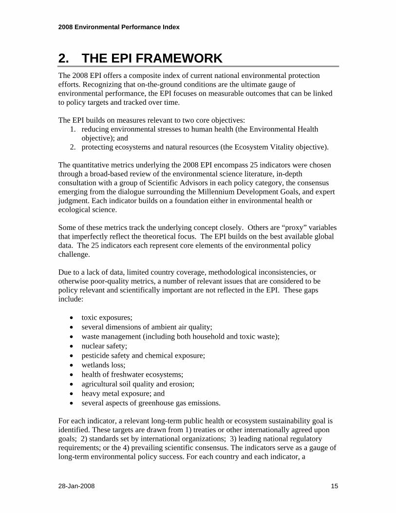
2. THE EPI FRAMEWORK The 2008 EPI offers a composite index of current national environmental protection efforts. Recognizing that on-the-ground conditions are the ultimate gauge of environmental performance, the EPI focuses on measurable outcomes that can be linked to policy targets and tracked over time. The EPI builds on measures relevant to two core objectives:
1. reducing environmental stresses to human health (the Environmental Health objective); and
2. protecting ecosystems and natural resources (the Ecosystem Vitality objective). The quantitative metrics underlying the 2008 EPI encompass 25 indicators were chosen through a broad-based review of the environmental science literature, in-depth consultation with a group of Scientific Advisors in each policy category, the consensus emerging from the dialogue surrounding the Millennium Development Goals, and expert judgment. Each indicator builds on a foundation either in environmental health or ecological science. Some of these metrics track the underlying concept closely. Others are “proxy” variables that imperfectly reflect the theoretical focus. The EPI builds on the best available global data. The 25 indicators each represent core elements of the environmental policy challenge. Due to a lack of data, limited country coverage, methodological inconsistencies, or otherwise poor-quality metrics, a number of relevant issues that are considered to be policy relevant and scientifically important are not reflected in the EPI. These gaps include:
• toxic exposures; • several dimensions of ambient air quality; • waste management (including both household and toxic waste); • nuclear safety; • pesticide safety and chemical exposure; • wetlands loss; • health of freshwater ecosystems; • agricultural soil quality and erosion; • heavy metal exposure; and • several aspects of greenhouse gas emissions.
For each indicator, a relevant long-term public health or ecosystem sustainability goal is identified. These targets are drawn from 1) treaties or other internationally agreed upon goals; 2) standards set by international organizations; 3) leading national regulatory requirements; or the 4) prevailing scientific consensus. The indicators serve as a gauge of long-term environmental policy success. For each country and each indicator, a

2008 Environmental Performance Index
28-Jan-2008 16
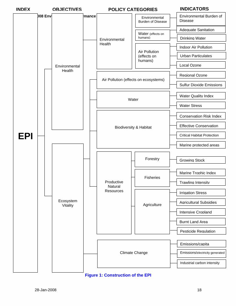
proximity-to-target value is calculated based on the distance from a country’s current results to the policy target. In calculating EPI scores, we average around isolated data gaps. But countries with more than a few missing data values (preventing any of our category scores from being calculated) are dropped from the Index. Our data matrix covers 149 countries for which an EPI can be calculated across the 25 indicators. Data gaps mean that another 90 or so countries that cannot be ranked in the 2008 EPI. Using the 25 indicators, scores are calculated at three levels of aggregation. See Figure 1. First, building on two to four underlying indicators (each representing a data set), we calculate scores for each of the six core policy categories – Environmental Health, Air Quality, Water Resources, Biodiversity and Habitat, Productive Natural Resources, and Climate Change. In some cases, subcategories are also tracked. The weight given to each indicator varies as shown in Table 1. This level of aggregation permits countries to track their relative performance within these well-established policy areas – or at the disaggregated indicator level. Second, the Environmental Health subcategories and the Ecosystem Vitality categories are aggregated with weights allocated as shown in Figure 1. Finally, the overall Environmental Performance Index is calculated, based on the arithmetic mean of the two broad objective scores. The logic for the weightings each subcategories and indicators is discussed below. 2.1. Indicator Selection and Targets Indicators were sought to cover the full spectrum of issues underlying each of the major policy categories identified. To ensure the use of the best suited metrics, the following indicator selection criteria were applied: Relevance: The indicator clearly tracks the environmental issue of concern in a way that
is relevant to countries under a wide range of circumstances. Performance orientation: The indicator tracks ambient conditions or on-the-ground
results (or is a “best available data” proxy for such outcome measures). Transparency: The indicator provides a clear baseline measurement, has the ability to
track changes over time, and is transparent with regard to data sources and methods. Data quality: The data used by the indicator should meet basic quality requirements and
represent the best measure available.

2008 Environmental Performance Index
28-Jan-2008 17
2.2. Data Gaps and Country Data Coverage The 2008 EPI builds on the best environmental data available, but remains seriously constrained by a lack of both quality and quantity in data sources. About 90 countries cannot be included in the EPI because data are not available in one of the six policy categories. Many critical issues also lack reliable measures. The 2008 EPI covers 149 of a possible 238 countries. Due to a lack of data, limited country coverage, methodological inconsistencies, or otherwise poor-quality metrics, a number of relevant issues that are considered to be policy relevant and scientifically important are not reflected in the EPI. These gaps include:
• toxic exposures; • several dimensions of ambient air quality; • waste management (including both household and toxic waste); • nuclear safety; • pesticide safety and chemical exposure; • wetlands loss; • health of freshwater ecosystems; • agricultural soil quality and erosion; • heavy metal exposure; and • several aspects of greenhouse gas emissions.
2008 Environmental Performance Index
28-Jan-2008 18
Figure 1: Construction of the EPI
INDICATORS
Urban Particulates
EPI
Environmental
Health
INDEX
Air Pollution (effects on ecosystems)
Productive Natural
Resources
Biodiversity & Habitat
Climate Change
Water
OBJECTIVES POLICY CATEGORIES
Indoor Air Pollution
Adequate Sanitation
Drinking Water
Environmental Burden of Disease
Local Ozone
Regional Ozone
Environmental Health
Sulfur Dioxide Emissions
Emissions/capita
Emissions/electricity generated
Industrial carbon intensity
Water Quality Index
Water Stress
Conservation Risk Index
Effective Conservation
Critical Habitat Protection
Marine protected areas
Growing Stock
Marine Trophic Index
Trawling Intensity
Irrigation Stress
Agricultural Subsidies
Intensive Cropland
Burnt Land Area
Forestry
Fisheries
Agriculture
Ecosystem Vitality
Environmental Burden of Disease
Water (effects on humans)
Air Pollution (effects on humans)
Pesticide Regulation

2008 Environmental Performance Index
28-Jan-2008 19
Table 1: Weights, Sources, and Targets of EPI Objectives, Categories, Subcategories, and Indicators
Index Objectives Policy Categories Subcategories Indicators Data Source Target
Environmental burden of disease (DALYs) 25% WHO 0 DALYs
Adequate sanitation 6.25%
WHO-UNICEF Joint Monitoring Program 100% Water (effects
on humans) 12.5% Drinking water 6.25% WHO-UNICEF Joint Monitoring
Program 100%
Urban particulates 5% World Bank, WHO 20 ug/m3 Indoor air pollution 5% WHO 0%
Environmental Health 50%
Air Pollution (effects on humans) 12.5%
Health ozone 2.5% MOZART II model 0 exceedance above 85 pbb
Ecosystem ozone 1.25% MOZART II model
0 exceedance above 3000 AOT40. AOT40 is cumulative exceedance above 40 ppb during daylight summer hours
Air Pollution (effects on ecosystems) 2.5%
Sulfur dioxide emissions 1.25% EDGAR/Netherlands 0 tons SO2 / populated
land
Water quality 1.25% UNEP GEMS/Water 100 score Water (effects on ecosystems) 7.5%
Water stress 1.25% UNH Water Systems Analysis 0% territory under water stress
Conservation risk index [7.5 / (2+AZE weight + MPAEEZ weight)]%
The Nature Conservancy 0.5 ratio
Effective conservation [7.5 / (2+AZE weight + MPAEEZ weight)]%
The Nature Conservancy 10%
Critical habitat protection* [if no AZE sites: 0; if AZE sites: 7.5 / (2+AZE weight + MPAEEZ weight)]%
Alliance for Zero Extinction, TNC 100%
Biodiversity & Habitat 7.5%
Marine Protected Areas* [minimum of 7.5*EEZ area / land area and 7.5, divided by (2+AZE weight + MPAEEZ weight)]%
Sea Around Us Project, Fisheries Centre, UBC 10%
EPI
Ecosystem Vitality 50%
Productive Natural Forestry* 2.5% Growing stock change FAO ratio of at least 1

2008 Environmental Performance Index
28-Jan-2008 20
Marine Trophic Index UBC, Sea Around Us Project no decline Fisheries* 2.5%
Trawling intensity UBC, Sea Around Us Project 0%
Irrigation Stress*
CIESIN calculation based on global irrigation map by Johann Wolfgang Goethe University and Food and Agriculture Organization of the UN, and water stressed area map by University of New Hampshire Water Systems Analysis Group
0%
Agricultural Subsidies World Bank, World Development Report 0
Intensive cropland CIESIN calculation based on global cropland grid from Ramankutty et al. (forthcoming)
0%
Burned Land Area
Joint Research Centre’s Global Burnt Areas 2000-2007 (L3JRC)CIESIN Global Rural-Urban Mapping Project (GRUMP) land area and country grids.
0%
Resources 7.5%
Agriculture* 2.5%
Pesticide Regulation UNEP-Chemicals
9 banned POP chemicals and full participation in Rotterdam and Stockholm Conventions
Emissions per capita IEA, CDIAC, Houghton
2.24 Mt CO2 eq. (Estimated value associated with 50% reduction in global GHG emissions by 2050, against 1990 levels)
Emissions per electricity generation IEA 0 g CO2 per kWh
Ecosystem Vitality 50%
Climate Change 25%
Industrial carbon intensity IEA, WDI
.85 tons of CO2 per $1000 (USD, 2005, PPP) of industrial GDP (Estimated value associated with 50% reduction in global GHG emissions by 2050, against 1990 levels)
*Averaged around if missing data or not applicable to country
2008 Environmental Performance Index
28-Jan-2008 21
2.3. Targets The EPI builds on a set of carefully chosen policy targets. Measuring success against these targets provides useful information about country-specific conditions and policy results, as well as areas in need of increased attention and resources. A proximity-to-target measure helps to clarify comparative rankings, demonstrate which countries are leading or lagging in each area, and whether (as a global aggregate) the world is on a sustainable trajectory. Whenever possible our targets are based on international treaties and agreements. For issues with no international agreements, we looked next to environmental and public health standards developed by international organizations and national governments, the scientific literature, and finally, expert opinion from around the world. Only a few of the indicators have explicit consensus targets established at a global scale. This suggests that there is also a need for the international and national policy communities to be clearer about the long-term goals of environmental policies set at all levels. International agreements are often based on compromises, however, and targets derived from them do not necessarily reflect environmental performance required for full sustainability. 2.4. Calculating the EPI To make the 25 indicators comparable, each metric was converted to a proximity-to-target-measure with a range of 0 to 100.
Initially, we examined the distribution of each indicator to identify whether extreme values skew the aggregations of some indicators. Our analysis concluded that the extreme values are more indicative of being “outliers”( values numerically much larger or smaller than the rest of the distribution) than of being the realizations of a skewed distribution. Accordingly we adjusted outliers using a recognized statistical technique called winsorization. In a small number of cases even this level of winsorization left significant outliers, and in such cases we winsorized at a greater level based on a comparison of the two alternative values (see Appendix E for Methodology details).
A second decision concerned the treatment of countries that exceeded the long-term performance or sustainability target. To avoid rewarding “over-performance,” no indicator values above the long-term target were used. In the few cases where a country did better than the target, the value was reset so that it was equal to the target. Once those two adjustments were made, a simple arithmetic transformation was undertaken: the observed values were placed onto a zero to 100 scale where 100 corresponds to the target and zero to the worst observed value. 2.5. Data Aggregation and Weighting Aggregation is an area of inescapable methodological controversy. While the field of composite index construction has become a well-recognized subset of statistical analysis,

2008 Environmental Performance Index
28-Jan-2008 22
there is no clear consensus on how best to construct composite indices. Various aggregation methods exist, and the choice of an appropriate method depends on the purpose of the composite indicator as well as the nature of the subject being measured. To help identify appropriate groupings and weights for each indicator, we carried out a principal component analysis (PCA). Most categories did not have clear referents in the PCA results. Absent a PCA-derived basis for weighting the indicators, equal weights were used with some refinements determined by the EPI team with expert guidance. The Environmental Health and Ecosystem Vitality subcategories each represent 50% of the total EPI score. This equal division of the EPI into issues related to (1) humans and (2) nature is not a matter of science but rather policy judgment. But this even weighting of the two overarching objectives of environmental policy reflects a broad-based institution – and this choice (used in the 2006 Pilot EPI) has not been generally criticized. Indeed, for every “deep ecologist” who favors more weight being placed on Ecosystem Vitality, there is a “humans first” environmental policymaker who prefers that the tilt go the other way. Within the Environmental Health subcategory, the Environmental Burden of Disease (DALY) indicator is weighted 50% and accordingly contributes 25% of the overall EPI score, because it is widely regarded to be the most comprehensive and carefully-defined available measure of environmental health burdens. The effects of Water and Air Pollution on human health comprise the remainder of the Environmental Health subcategory and are each allocated a quarter of the total score for Environmental Health, reflecting a widespread policy consensus. The two water-related indicators (Adequate Sanitation and Drinking Water) are equally weighted. Urban Particulates and Indoor Air Pollution receive equal weights, and double the weight given to the effects of ground-level Ozone on human health. Urban Particulates and Indoor Air are widely acknowledged by the United Nations Environment Programme (UNEP), World Health Organization (WHO), and United Nations Children’s Fund (UNICEF) as excellent indicators of the burden of air pollution on human health. There is, however, a growing literature that suggests a link between ozone exposure and human health. Our human-exposure-related ozone metric builds on ozone exposure modeled by Denise Mauzerall and her colleagues on the global chemical transport Model of Ozone and Related Tracers, version 2 (MOZART-2). Because this indicator is experimental, we give it half the weight of those with known reliability. Within the Ecosystem Vitality subcategory, the Climate Change indicator carries 50% of the subcategory’s weight (i.e., 25% within the total EPI). The Air Pollution indicator is weighted to 2.5% of the subcategory total, due to the statistical variance of the datasets and the understanding that policymakers find water issues more fundamental than air pollution to ecosystem vitality. The remaining indicators: Water, Biodiversity, and Productive Natural Resources, are each evenly weighted to cover the remaining 22.5% of the subcategory.
2008 Environmental Performance Index
28-Jan-2008 23
3: RESULTS AND ANALYSIS The 2008 EPI provides policymakers and environmental experts an empirically grounded basis for comparing the environmental performance of nearly 150 countries worldwide. While general trends exist, such as a correlation between wealth and strong environmental health performance, some countries perform beyond income-based expectations. The results highlight policy leaders and laggards. They also provide a basis for identifying environmental “best practices.” The top five ranked countries in the 2008 EPI, in order of best performance, are Switzerland, Sweden, Norway, Finland, and Costa Rica. As expected, developed countries with significant financial resources for environmental management make up a large portion of top performers. But Costa Rica, a middle-income country, outperforms many developed countries as well as its neighbors. The bottom five countries in the 2008 EPI in order of performance are Niger, Angola, Sierra Leone, Mauritania, and Mali, are all located in Sub-Saharan Africa and lack resources for even basic environmental investments. Overall there were many more high performing countries in the Environmental Health arena than in Ecosystem Vitality. Sixty-six countries had scores of 90 or above in Environmental Health, whereas only 2 scored above 90 in Ecosystem Vitality. The number of high performers in Environmental Health reflects government attention to basic human needs, such as drinking water and sanitation. Unlike Ecosystem Vitality, Environmental Health is highly correlated with wealth, indicating that many of the low-performing countries have not made the requisite investment in baseline environmental amenities. Because so many countries had high Environmental Health scores, especially among the top countries, a low performance in Ecosystem Vitality had the ability to reduce a country’s rank substantially. Countries such as Australia, Belgium, and the United States, which have Environmental Health scores at above 98, perform well below many members of their peer groups in the EPI because of their substantially lower Ecosystem Vitality scores. Performance in Ecosystem Vitality is more normally distributed than the performance in Environmental Health. In part, this reflects the fact that Ecosystem Vitality is a composite of many different indicators, which tends to spread those scores. Countries that scored well in ecosystem vitality often did so for very different reasons. Of the two countries with scores above 90, Switzerland’s performance can be primarily attributed to good environmental management whereas Laos’s high score arises from a lack of development and limited stress on the land, air, and water. Countries falling in the middle of the rankings vary considerably. Some low-ranked countries, such as Kuwait, at 111th position, have an Environmental Health scores above 90. This result suggests they have on-going struggles with one or more of the ecosystem

2008 Environmental Performance Index
28-Jan-2008 24
vitality policy categories. Likewise, Laos, despite its top ecosystem vitality score, ranks at 101 in the EPI because of a very low environmental health score. The United States, though very high in the Environmental Health score, ranked at 107th in the Ecosystem Vitality category, below countries like Sudan and Myanmar, which have significant non-environmental challenges and limited resources for environmental protection. Poor performance in the areas of air emissions and climate change reduced the United States’ score significantly. China and India, containing about one third of the world’s population, received similar low Ecosystem Vitality scores. Both countries were ranked in the bottom third of the index. However China scored higher in the overall EPI because of its improved Environmental Health score. 3.1. EPI Results by peer group The overall EPI results offer a useful snapshot of environmental performance. But breaking down the results into peer groups offers an even more valuable perspective because it allows for comparisons between countries. The peer group analysis gives policymakers a way to understand the context of their policy choices and guidance on what is possible in the way of policy results given their circumstances. The policies and programs of the peer group leaders present an important guide to best practices and the most efficient approaches to improving environmental health and ecosystem vitality with similar challenges and opportunities. OECD countries occupy four of the top five ranks in the 2008 EPI. Most of the OECD countries are in the top quarter of the Index, and all are in the top half. These relatively wealthy countries all have quite good Environmental Health results. But their scores on the various metrics of Ecosystem Vitality vary widely. Some of these nations, notably the Scandinavians, have distinct geographic advantages, including large land areas and low population densities. But their success is also a function of concerted policy effort and deep commitment to environmental values across their public and business communities. None of the Least Developed Countries (LDC) were in the top half of the EPI, and the bottom 14 countries in the EPI are found in this group. With little access to financial resources for immediate needs like nutrition and disease, many of these countries are struggling to make even baseline efforts on environmental health. Their lack of development translates into limited pollution stress and thus contributes to relatively strong scores on air emissions, climate change, and biodiversity. High population density countries are spread throughout the EPI. Germany, for example, sits in the 13th position while Burundi ranks 132nd. High populations density generates special challenges, but the high-ranked performers in this category demonstrate that population density is not an insurmountable barrier to good environmental quality. Many of the lower ranked countries in this grouping face challenges, but can look to their higher ranking peers for guidance on how to develop in an environmentally sustainable manner. Other peer groups, like the African Union, the Alliance of Small Island States, the Desert Countries, and the Newly Independent States contain are spread across the EPI. Each of these peer groups is largely populated by developing countries that struggle with a wide

2008 Environmental Performance Index
28-Jan-2008 25
variety of challenges, including a lack of natural resources like water and arable land, as well as the burden of poverty. Overall, these peer groups show much more diversity than do groupings like the OECD and the LDCs. This result implies that countries in the midst of economic transitions vary widely in how well they fold environmental protection into their development strategies.

2008 Environmental Performance Index
28-Jan-2008 26
5. SENSITIVITY ANALYSIS
Michaela Saisana and Andrea Saltelli, Econometrics and Applied Statistics Group, Institute for the Protection and Security of the Citizen, Joint Research Centre of the European Commission Summary An assessment of the robustness of the 2008EPI results requires the evaluation of uncertainties underlying the index and the sensitivity of the country scores and rankings to the methodological choices made during the development of the Index. To test this robustness, the EPI team has continued its partnership with the Joint Research Centre (JRC) of the European Commission in Ispra, Italy. A summary of the JRC sensitivity analysis follows. The more detailed version is included in the Appendix.
Any composite indicator, such as the EPI, involves subjective judgments such as the selection of indicators, the data treatment, choice of aggregation method, and the weights applied to the indicators. Because the quality of an index depends on the soundness of its assumptions, good practice requires evaluating confidence in the index and assessing the uncertainties associated with its development process. To ensure the validity of the policy conclusions extracted from the EPI, it is important that the sensitivity of the index to alternative methodological assumptions be adequately studied. Sensitivity analysis permits the examination of the framework of a composite index by looking at the relationship between information flowing in and out of it (Saltelli et al. 2008). Using sensitivity analysis, we can study how variations in EPI scores and ranks derive from different sources of variation in the assumptions. Sensitivity analysis also demonstrates how each indicator depends upon the information that composes it. It is thus closely related to uncertainty analysis, which aims to quantify the overall uncertainty in a country’s score (or rank) as a result of the cumulative effect of uncertainties in the index construction. A combination of uncertainty and sensitivity analyses can help to gauge the robustness of the EPI results, to increase the EPI’s transparency, to identify the countries that improve or decline under certain assumptions, and to help frame the debate around the use of the index.
The validity of the EPI scoring and respective ranking is assessed by evaluating how sensitive it is to the assumptions that have been made about its structure and the aggregation of the 25 underlying indicators. The sensitivity analysis carried out for EPI is mainly related to:
1. the measurement error of the raw data, 2. the choice of capping at selected targets for the 25 indicators, 3. the choice to correct for skewed distributions in the indicators values, 4. the weights assigned to the indicators and/or to the subcomponents of the index,
and finally 5. the aggregation function at the policy level.
The main conclusions are summarized below.

2008 Environmental Performance Index
28-Jan-2008 27
How do the EPI ranks compare to the ranks under alternative methodological approaches? The frequency table of a country’s rank summarizes the position a country can take anywhere in the 149-rank ladder (grouped in blocks of ten) when accounting for different combinations of the five types of uncertainty mentioned previously. A total of 40,000 simulations were run in order to cover the space of uncertainties present in the 2008 EPI. We discuss ranks and not scores because non-parametric statistics are more appropriate in our case given the non-normal character of the data and the scores. In the relevant literature, the median rank is proposed as a summary measure of a rank distribution. The median rank of all combinations of assumptions indicates that for 1 out of 2 countries in the EPI, the difference between the EPI rank and the most likely (median) rank is less than 15 positions (recall that we have a total of 149 studied countries). Thus, for half of the countries studied, the modest sensitivity of the EPI ranking to the five assumptions (eventual measurement error in the raw data, the correction of skewed data distribution, the use of target values, the weighting of the indicators, and finally the aggregation function at the policy level) implies a reasonably high degree of robustness of the index for those countries. For the remaining half of the countries, the EPI performance is highly sensitive to the methodological choices in the index, and should thus be considered as merely indicative. A discussion on the top performing countries is in place. The top ten performing countries in the EPI include Switzerland, Sweden, Norway, Finland, Costa Rica, Austria, New Zealand, Latria, Colombia and France. However, the simulations indicate that most of those countries should be positioned much lower. Switzerland, for example has a probability of only 31% to be ranked in the top ten countries, whilst even lower is the probability for Austria, Latvia and France. In our simulations, New Zealand scores 98% of the times in the top ten, followed by Finland, Costa Rica and Colombia. Panama, whose EPI rank is 32, should actually be considered as a top ten performing country, given that its score is among the top ten in 73% of the simulations.
Which are the most volatile countries and why? There are several countries with a relatively high difference between their best and worst rank. A very high volatility of more than 80 positions is found for Hungary (rank: 23), Denmark (25), Albania (27), Ireland (34), Uruguay (36), Bosnia & Herzegovina (48), Belgium (57), El Salvador (65), Laos (101) and Tanzania (113). The volatility of those countries is due to the combined effect of all five assumptions, although the most influential input factors are the (1) use of a geometric versus a arithmetic average aggregation function at the policy level and (2) the use of equal weighting or Factor Analysis weighting at the indicators level.
What if measurement error is incorporated? A normally distributed random error term was added to the raw data with a mean zero and a standard deviation equal to the observed standard deviation for each indicator. Among the countries that are most affected by this assumption is Luxembourg (rank: 31), whose rank would drop by 53 positions. On the other extreme, the Philippines (rank: 61) would improve its rank and be placed in the 10th position. Overall, the introduction of measurement error in the raw data has a median impact of 9 ranks and a 90th percentile

2008 Environmental Performance Index
28-Jan-2008 28
impact of 29 ranks. In other words, this assumptions leaves 1 out of 2 countries almost unaffected (less than 9 rank change), but 1 out of 10 countries would shift more than 29 ranks.
What if skewed distributions are not winsorized? Winsorization was not found to have a significant impact on the EPI ranking. Most notably, Luxembourg (rank: 31) would deteriorate its rank by 53 positions. On the other extreme, the Philippines (rank: 61) would improve its rank and be placed in the 10th position. Overall, the introduction of measurement error in the raw data has a median impact of 9 ranks and a 90th percentile impact of 29 ranks. In other words, this assumptions leaves 1 out of 2 countries almost unaffected (less than 9 ranks change), but 1 out of 10 countries would shift more than 29 positions.
What if capping at target values for the indicators is not undertaken? Luxembourg (rank: 31) and Laos (rank: 101) would see the greatest shift in their ranks (a decline of 12 and 15 positions respectively). In the best case, El Salvador (rank: 65) will improve by 9 positions. Overall, for 1 out of 2 countries, the impact of this assumption is only 3 positions, while 1 out of 10 countries shift by more than 7 positions, but not more than 15. Thus, the impact of capping at the indicators’ performance targets exerts only a small impact on the EPI ranking.
What is the impact of alternative weighting schemes? Four alterative weighting schemes, all with their implications and advantages, are deemed as the most representative in the literature of composite indicators and worth being tested in our current analysis. • current weighting vs. FA-derived weights at the indicator level; • current weighting vs. equal weighting at the indicator level; • current weighting vs. equal weighting at the subcategory level; • current weighting vs. equal weighting at the policy level; The simulation study showed that all of these scenarios have significant influence on the EPI ranking (see Appendix on Sensitivity Analysis for full detail). The scenarios with the biggest effect being equal weighting at the policy level, equal weighting at the indicator level, and Factor Analysis derived weights at the indicator level. In any of these three cases, 1 out of 2 countries shifts less than 15 positions with respect to the original EPI ranking, whilst 1 out of 10 countries shifts more than 50 positions.
What if the aggregation function is geometric instead of arithmetic? When a non-compensatory aggregation is performed at the policy level using the geometric mean function instead of the arithmetic mean, the effect on the EPI rankings is moderate. Sri Lanka, Peru and Egypt improve their ranks by 18 positions or more, whilst the greatest decline is observed for Uruguay (down more than 51 positions). Overall, for 1 out of 2 countries, the impact of this assumption is merely 5 positions, while 1 out of 10 countries shift by more than 18 positions (up to 51 positions).

2008 Environmental Performance Index
28-Jan-2008 29
All things considered, the 2008 EPI has an architecture that highlights the complexity of translating environmental stewardship into straightforward, clear-cut policy recipes. The trade-offs within the index dimensions are a reminder of the danger of compensability between dimensions while identifying the areas where more work is needed to achieve a coherent framework in particular in terms of the relative importance of the indicators that compose the EPI framework.

2008 Environmental Performance Index
28-Jan-2008 30
APPENDIX D: THE 2008 EPI, PILOT 2006 EPI, AND ENVIRONMENTAL SUSTAINABILITY INDEX D.1. Comparison of the Pilot 2006 Environmental Performance Index and the 2008 Environmental Performance Index Both the Pilot 2006 EPI and the 2008 EPI are outcome-oriented performance indices. Like the 2006 Pilot EPI, the 2008 EPI is an attempt to assess current environmental conditions to provide policymakers with information they can use now in forming and assessing policy responses to environmental challenges. Both indices use a proximity-to-target approach to assess countries’ performance on accepted targets for environmental sustainability where governments can have an immediate effect on efforts to improve environmental conditions. While following the same general principles of construction and interpretation, i.e., a multi-tier aggregation of proximity-to-target indicators, the 2008 EPI differs from the pilot index in several structural and substantive areas. Structurally, the 2008 EPI’s Environmental Health and Productive Natural Resources categories are further broken down into sub-categories to reflect the thematic similarities between the underlying indicators and allow for a more appropriate weighting scheme. Overall, the number of indicators has increased to 25 compared to 16 in Pilot 2006 EPI. The 2008 EPI now presents a more thorough inclusion of data that provide information on a wider variety of environmental indicators. Furthermore, the 2008 EPI does not use the hybrid weighting of the Pilot 2006 EPI, which combines statistically derived weights from Principal Component Analysis with weights reflecting the combined judgment of experts and policymakers. The reasons for this methodological change do not mean we are abandoning the application of rigorous statistical principles in the index’s design but the need for a nuanced and balanced compromise between what the data are telling us on the one hand and what is sensible from a policy perspective on the other3. A third methodological change compared to the Pilot 2006 EPI is the very limited and controlled use of missing data imputation to fill data gaps. Since one of our guiding principles is to offer a globally relevant and applicable performance assessment tool, data coverage is of paramount importance. Unfortunately, the inclusion of more advanced indicators in the 2008 EPI often comes at the expense of geographical coverage. For this reason, we have used a suite of imputation methods, including regression and correlation analysis, to increase country coverage in these indicators: Adequate Sanitation, Drinking 3 Although PCA weights reflect the importance, expressed as fractions of variation in the data that can be explained, of an indicator relative to others with respect to the principal component(s), these weights are not always representative of the policy attention given to an environmental issue. In addition, since the PCA weights depend on the data, their reliability depends on the quality of the data and, furthermore, subsequent releases of the index would with high likelihood result in different weights, which does not generally coincide with changes in policy attention.

2008 Environmental Performance Index
28-Jan-2008 31
Water, Indoor Air Pollution, Water Quality Index, GHG Emissions Per Capita, CO2 Emissions per Electricity Generated, and Industrial Carbon Intensity. Since these imputed values may reflect the true but unknown values to varying degrees of accuracy, we have clearly marked them in the data tables. Substantively, the 2008 EPI demonstrates our commitment to identifying the best available and developing the best possible environmental performance indicators that are currently available at the global level. We believe that the new 2008 EPI is a continued improvement and makes a significant contribution to environmental performance assessment. Specifically, the 2008 EPI has improved upon the 2006 EPI in the environmental health area through the use of Disability Adjusted Life Years (DALY’s), which more fully capture the effect of environmental conditions on human health and productivity than the child mortality indicator in the Pilot EPI. This year’s EPI also more fully captures the effects of air pollution on both human health and the environment, adding indicators for sulfur dioxide pollution and separating the health and ecological effects of ground-level ozone according to scientific evidence and large-scale tempo-spatial modeling results. We have further strengthened the water indicators, primarily by advancing the measurement of water quality with information on pH, dissolved oxygen, conductivity, and total phosphorus in addition to the 2006 EPI’s inclusion of data on nitrogen. Perhaps one of the biggest changes in the 2008 EPI is the weight placed on the new Climate Change category, which absorbs the 2006 EPI’s Sustainable Energy category, and the additional data included in its calculation: GHG Emissions Per Capita, CO2 Emissions Per Electricity generated, and Industrial Carbon Intensity. Because of the greater recognition of climate change as one of the most pressing environmental challenges, the 2008 EPI weights climate change much more heavily in the ecosystem vitality objective. As a result, countries with otherwise advanced environmental regulatory and enforcement systems such as the United States and Australia, dropped in this year’s EPI in part because of this expanded category. Biodiversity, Agriculture, and Fisheries were all improved with new and more sophisticated indicators in this year’s EPI. The Agriculture category includes measures assessing intensive cropland coverage, pesticide regulations, irrigation stress, and burned land area in addition to the agricultural subsidy data included in the 2006 EPI. The subsidies data have also been improved in their consistency and extent by tapping into an expanded data source. The Fisheries category assesses Trawling intensity and the Marine Trophic Index compared to the overfishing indicator used in the 2006 Pilot EPI. Finally, the Biodiversity and Habitat category offers a completely new suite of advanced conservation and threat measures including the Conservation Risk Index and assessments of the Effectiveness of Conservation Efforts, Critical Habitat Protection, and – importantly – Marine Protected Areas. Despite the progress made in indicator development and data availability, the 2008 EPI continues to highlight the glaring gaps in global environmental data. Several important environmental concerns such as population exposure to pollutants and toxins, trans-national outsourcing and spill-over effects of ‘dirty’ industries, and the effects of

2008 Environmental Performance Index
28-Jan-2008 32
widespread human activities on locally sensitive conditions (e.g., critical loads of sulfur dioxide deposition) still cannot be measured adequately at the global level because of lack of data, targets, and/or scientific certainty. Although the 2008 EPI contains 149 countries, many countries are not included because of the lack of information about key indicators, despite our efforts to produce meaningful imputations. This makes tracking and monitoring of environmental progress and success of policy and management efforts difficult, and although the 2008 EPI improves upon the 2006 EPI, much work remains to be done in establishing consistent data collection and monitoring of environmental metrics. D.2. Comparison of the Environmental Sustainability Index and the Environmental Performance Index Between 1999 and 2005 the Yale and Columbia team published four Environmental Sustainability Index reports aimed at gauging countries’ overall progress towards ‘environmental sustainability’. Since then our focus has shifted to environmental performance, measuring the ability of countries to actively manage and protect their environmental systems and shield their citizens from harmful environmental pollution. Why this shift in our work? While sustainability research continues at a fast pace across the world, a commonly accepted and measurable definition of environmental sustainability remains elusive. Distinct approaches have emerged and consolidated within different disciplines, and cross-disciplinary exchange has promoted new advances, but the challenges are still formidable. In addition, the immediate value to policymakers was limited by the complexity of the problem, scientific uncertainties about cause-effect relationships, and the intricate and competing linkages between policy actions and the social, economic, and environmental aspects of sustainable development. In contrast, environmental performance offers a more relevant and easily measured approach to reducing our societal environmental impacts. The possibility of selecting outcome-oriented indicators for which policy drivers can be identified and quantified is an appealing scenario for policymakers, environmental scientists and advocates, and the public alike. This method promotes action, accountability, and broad participation. The EPI’s proximity-to-target approach in particular highlights a country’s shortcomings and strengths compared to its peers in a transparent and easily visualized manner. These signals can be acted on through policy processes more quickly, more effectively, and with broader consensus than most sustainability metrics. In some cases, the EPI targets can already be viewed as sustainability targets, while other indicators represent the most widely accepted or most stringent agreed-upon policy goals. Aside from these main conceptual and structural differences, how exactly do the EPI and ESI differ from each other? A summary of the differences is shown in Table A for the 2005 ESI, 2006 Pilot EPI, and 2008 EPI. In contrast to the relative measurements of the ESI, the EPI is a benchmark index. The sustainability thresholds of many environmental and socio-economic aspects are extremely difficult to determine and, given the dynamics of human and ecological change,

2008 Environmental Performance Index
28-Jan-2008 33
might not exist in an absolute sense. The ESI evaluates environmental sustainability relative to the paths of other countries. The EPI, on the other hand, uses the distance to performance targets as the main criteria, acknowledging that these targets represent imperfect goalposts and can depend on local circumstances. Although both the EPI and ESI are multi-tier, average-based indices, they significantly differ in the categories of which they are composed. In line with sustainability research, the ESI considers not only environmental systems but also adapts the Pressure-State-Response framework to reflect institutional, social, and economic conditions. The EPI, in contrast, considers only ecological and human health outcomes regardless of the auxiliary factors influencing them. The basic premise of the EPI is therefore normative. Each country is held to the same basic conditions necessary to protect human and environmental health now and in the future. The benchmarks for these conditions are enshrined in the 25 indicator targets. As a result of the EPI’s narrowed scope, the categories and indicators tracked are both different and smaller in number. Data quality and coverage play important roles in both the EPI and ESI. We believe that the value of a sustainability and performance index is diminished if only a handful of countries can be included and compared. Yet, while the ESI makes relatively extensive use of imputation techniques to fill data gaps, the availability of actual ‘real’ data was given much higher weight in the EPI to reflect the relevance of observed data in the policy process (2008 EPI does impute missing values in selected variables to maintain country coverage). As our knowledge of cause-effect relationships and statistical methods for data imputation continues to increase, however, it is likely that model-based imputations will gain more credibility in the future and in some cases even outperform real observations in accuracy. Table A: Comparison of ESI and EPI objectives and design Category 2005 ESI 2006 EPI 2008 EPI Objective Gauges the long term
environmental trajectory of countries by focusing on “environmental sustainability”
Assesses current environmental conditions
Assesses current environmental conditions
Design Provides a relative measure of past, current, and likely future environmental, socio-economic, and institutional conditions relevant to environmental sustainability
Provides an absolute measure of performance by assessing countries on a proximity-to-target basis
Provides an absolute measure of performance by assessing countries on a proximity-to-target basis
Design and theoretical framework
Tracks a broad range of factors that affect sustainability using an adaptation of Pressure-State-Response framework
Focuses narrowly on areas within governmental control using a framework of absolute, fixed targets
Focuses narrowly on areas within governmental control using a framework of absolute, fixed targets

2008 Environmental Performance Index
28-Jan-2008 34
Structure Multi-tier consisting of 5 components: Environmental systems, Reducing environmental stresses, Reducing human vulnerability, Social and institutional capacity, Global stewardship undergirded by 21 indicators and 76 variables (Note: the variables in the ESI can be compared with indicators in the EPI and indicators in the ESI are more reflective of the categories in the EPI)
Multi-tier consisting of 2 objectives: Environmental health and Ecosystem vitality, 6 categories: environmental health, air quality, water resources, biodiversity and habitat, productive natural resources, and sustainable energy, and 16 indicators
Multi-tier consisting of 2 objectives: Environmental health and Ecosystem vitality, 6 categories: environmental health, air quality, water resources, biodiversity and habitat, productive natural resources, and climate change, and 25 indicators
Data quality and coverage
Stringent grading system; flexible data requirements allow for missing data to be imputed
Stringent data quality requirements, no imputation of missing data
Stringent data quality requirements; imputation of missing data in selected indicators
Environmental Health (EPI objective, ESI indicator)
Indicators compare mortality rates of environmentally related diseases using proxy indicators: child mortality, child death from respiratory diseases, and intestinal infectious diseases
Estimates environmentally-related impacts on health through child mortality, indoor air pollution, urban particulates concentration, access to drinking water, and adequate sanitation
Estimates environmental burden of disease directly using WHO-developed disability adjusted life year (DALYs), local ground-level ozone and urban particulate concentrations, indoor air pollution, access to drinking water, adequate sanitation
Air pollution Measures effects of air pollution as well as levels of air pollution: Coal consumption per capita, anthropogenic NO2, SO2, and VOC emissions per populated land area, and vehicles in use per populated land area
Measures air quality: Percent of households using solid fuels, urban particulates and regional ground-level ozone concentration
Measures atmospheric conditions pertaining to both human and ecological health: Health – Indoor air pollution, urban particulates, local ozone Ecosystems – Regional ozone, sulfur dioxide emissions (as proxy for its ecosystem impacts when deposited)
Water Resources and stress
Measures both water resources and stress: Quantity - Freshwater per capita and internal groundwater per capita Reducing stress – BOD emissions per freshwater, fertilizer and pesticides consumption per hectare arable land, percentage of country under water stress
Measures both water resources and stress: water consumption and nitrogen loading
Measures water stress through water stress index

2008 Environmental Performance Index
28-Jan-2008 35
Water Quality Key water quality indicators: dissolved oxygen, electrical conductivity, phosphorus concentration, suspended solids
Proxy for water quality: nitrogen loading.
Assesses water quality through composite Water Quality Index, which incorporates dissolved oxygen, pH, electrical conductivity, total nitrogen and total phosphorous concentrations
Climate Change / Energy
Tracks emissions per capita and per GDP Eco-efficiency indicator includes a measure of energy efficiency and renewable energy
Links energy to climate change via CO2 emissions per GDP, percent of renewable energy and energy efficiency
Explicitly assesses contributions to climate change through Emissions per capita, emissions per electricity generated, and industrial carbon intensity
Biodiversity & Habitat
Focuses on species protection: Percentage of threatened birds, mammals, and amphibians in a country, the National Biodiversity Index (measures species richness and abundance), and threatened ecoregions
Focuses on biome and resource protection: Wilderness protection, ecoregion protection, timber harvest rate, and water consumption
Focuses on biome protection, including marine areas, and species conservation through Effective conservation, Conservation Risk Index, and critical habitat protection, indicators
Forests Proxies for sustainable forest management: Annual change in forest cover and Percentage of total forest area that is certified for sustainable management
Proxy for sustainable forest management: Timber harvest rate
Proxy for sustainable forest management: Change in growing stock
Agriculture Proxy for sustainable agriculture: Agricultural subsidies
Proxy for sustainable agriculture: Agricultural subsidies
Proxies for sustainable agriculture: Agricultural subsidies, Intensive cropland usage, Pesticide regulations, and Burned land area
Fisheries Proxy for sustainable fisheries management: Overfishing
Proxy for sustainable fisheries management: Overfishing
Proxy for sustainable fisheries management: Trawling intensity, Marine Trophic Index

2008 Environmental Performance Index
28-Jan-2008 36
APPENDIX E: METHODOLOGY & MEASUREMENT CHALLENGES We believe that transparency is essential for good analysis, and aids concrete policy targets. This appendix provides a detailed description of the steps included in calculating the 2008 EPI and the statistical techniques used. The issues addressed in the following sections mirror those commonly encountered in the computation of composite indices: indicator and country selection, missing data treatment, standardization, aggregation and weighting methodologies, as well as performance testing (OECD, 2003).
E.1. Country Selection Criteria Ideally, the EPI should include all of the world’s countries and territories. However, persistent data gaps require that we balance geographical coverage against the validity and accuracy of available data. Wherever possible, and in line with our goal of providing a reliable and accurate picture of environmental performance of every country in the set, the 2008 EPI contains only countries with complete data coverage across all indicators and policy categories, with the following exceptions:
• Inclusion in the Fisheries indicator requires that countries have at least one of the two constituent indicators (Trawling Intensity and Marine Trophic Index).
• Inclusion in the Productive Natural Resource policy category requires countries to have at least two of the three constituent indicators (Forestry, Fishery, Agriculture). First, for some indicators – such as those in the Productive Natural Resources category, data availability depends in part on a country’s geographical location. Countries with no forests, no active fishing fleets and industries and no land used in agriculture may be missing some indicators associated with those activities but should be, and are, still included in the EPI.
• We imputed values for some countries for three indicators in the Environmental Health policy category: Drinking Water, Adequate Sanitation and Environmental Burden of Disease; Water Quality in the Water category; Agriculture Subsidies in the Productive Natural Resources category; as well as the indicators in the Climate Change category. In the case of the Drinking Water and Adequate Sanitation data there is a very high correlation between the indicator data and a rich body of literature and practitioners’ knowledge on the relationships between these measures and development. This knowledge base permits us to use available data to impute any missing values. The table below includes the complete list of indicators for which date were either averaged or imputed:

2008 Environmental Performance Index
28-Jan-2008 37
Indicator Name Indicator Code Missing Data Method Environmental Burden of Disease
DALY Imputation based on income per capita T
Adequate Sanitation ACSAT Imputation based on income per capita (log) and WATSUPa
Drinking Water WATSUP Imputation based on income per capita (log)
Water Quality WATQI Imputation based on regional average and non-reporting penalties
Critical Habitat Protection
AZE averaged around for countries with no AZE sites
Growing Stock Change FORGRO Imputation based on percentage change in forest cover 2000-2005.
Marine Protected Areas MPAEEZ averaged around for countries with no EEZ
Irrigation Stress IRRSTR averaged around for countries with no agricultural land
Intensive Cropland AGINT averaged around for countries with no agricultural land
Greenhouse Gas Emissions Per Capita
GHGCAP GHG emission imputation based on CO2 (CDIAC); Land emission imputation based on regional average of emissions per square kilometer
Agricultural Subsidies AGSUB Imputations based on 2006 EPI’s AGSUB proximity-to-target score. Missing 2008 AGSUB values were given scores that correspond to equivalent proximity-to-target scores
Emissions per Kilowatt Hour of Energy Produced
CO2KWH Imputations based on renewable energy as a percentage of all energy production.
Industrial Carbon Intensity
CO2IND Imputations CO2 emissions per GDP
E. 2. Target Selection
An additional challenge arises from the difficulty of determining clear performance targets for some of the indicators. For instance, in Europe, sulfur dioxide emission targets are based on sophisticated monitoring and modeling exercises that permit detailed, differentiated targets that take into account differences in emission trajectories, deposition sensitivities, and mitigation costs. There is no corresponding information base for assigning differential targets on a global basis, nor has there been any similar negotiating process to lend such targets legitimacy and authority. Therefore, our global target on sulfur dioxide (reduction to zero) is cruder than we would expect a fully mature global sulfur dioxide policy regime to adopt. Nonetheless, we consider such crude targets useful for the purpose of broad comparison among countries, both within single issues and collectively across multiple issues.

2008 Environmental Performance Index
28-Jan-2008 38
E.3. Missing Data
Despite improvements, data gaps remain a very serious obstacle to a more refined EPI and to data-driven policymaking more generally, Many countries, particularly in the developing world, lack data on a number of critical indicators. More generally, persistent data gaps, lack of time series data, or incomparability of data across countries means that several important policy challenges cannot be addressed adequately at present. For instance, air quality indicators based on ground-monitoring are unavailable for many developing countries and are further limited by weak data comparability even in developed countries, which combined with the dependency of conditions on local environmental and/or socio-economic characteristics severely reduces possibilities to impute data from one location to another.
Missing data is a major source of uncertainty in index construction. Although increasingly sophisticated statistical methods exist for imputing missing data, they entail assumptions regarding the causes for the missing values. In addition, application of these methods requires knowledge and careful consideration of the strengths and weaknesses of various techniques in light of the available data. To continue the air pollution example, such data are highly dependent on spatial and temporal conditions, which complicate the development of imputation models that are applicable to different regions and countries. In addition, the essence of the EPI—as a gauge of actual environmental results—requires particular confidence that any numbers imputed reflect ground-level circumstances and outcomes. We have used well-recognized imputation models to impute missing data for a number of indicators, as noted above.
Still, the lack of data leads limits the comprehensiveness of the EPI. In the air pollution context, pollutants such as lead, ultra-fine particulate matter (PM2.5), and volatile organic compounds (VOCs) do not have sufficient ground observations available and are not updated on a sufficiently frequent basis to permit robust performance metrics. Although satellite-based observation of air pollutants is advancing rapidly and provides more reliable estimates to fill in the gaps, availability and use of these technologies is still constrained. The result of these data gaps and inconsistencies is that only measures of regional ozone and sulfur dioxide emissions are included in the 2008 EPI to represent the ecological dimension of air pollution. The lack of adequate data indicates the need for increased national and international efforts to improve the same, specifically regarding better air quality measures.
More work remains to be done to both address the lack of available information on environmental policy issues and reduce serious shortcomings in the quality, geographical coverage, or timeliness of the available data. Since the publication of the Pilot 2006 EPI, we have been able to compile data for the crucial issues of biodiversity and conservation measures, fisheries data, and climate challenge. On the other hand, we are still calling on organizations and governmental bodies involved in environmental monitoring and data collection to invest in initiatives to assemble measures for many fields and issues including:
• Concentrations of additional criteria air pollutants • Exposure to toxic chemicals

2008 Environmental Performance Index
28-Jan-2008 39
• Blood lead levels • Soil degradation • Sector-specific greenhouse gas emissions • Pesticide application • Effectiveness of protected area management • Deposition of sulfur dioxide compare to critical loads
We hope that increased initiative will make it possible to fill these data gaps in the future.
E. 4. Calculation of the EPI and Policy Category Sub-Indices
Indicator Transformation for Cross-Country Comparisons
Environmental data are measured on various scales and require standardization to permit cross-country comparisons. Standardization also ensures that no indicator dominates the aggregated EPI and policy indices, and conveys information about a country’s environmental performance in an easy-to-understand yet meaningful way using a scale that quickly reveals a country’s position vis-à-vis other countries as well as with respect to desirable performance outcomes. For these reasons, the 2008 EPI– as in the Pilot 2006 EPI – uses a proximity-to-target approach that evaluates how close a country is to a desirable performance target for each of the 25 indicators.
Initially, we examined the distribution of each indicator to identify whether extreme values skew the aggregations of some indicators. Our analysis concluded that the extreme values are more indicative of being “outliers”( values numerically much larger or smaller than the rest of the distribution) than of being the realizations of a skewed distribution. Accordingly we adjusted outliers using a recognized statistical technique called winsorization. Winsorization essentially involves setting values falling below the 2.5th percentile to the 2.5 percentile value, and values above the 97.5th percentile equal to the 97.5th percentile. In a small number of cases even this level of winsorization left significant outliers, and in such cases we winsorized at the 5.0 or 95.0 percentile. Our decision rule for moving to this greater level of winsorization was based on a comparison of the two alternative values. If the ratio of the 97.5 percentile value to the 95 percentile value (or the 5.0 percentile value to the 2.5 percentile value) was greater than 5, indicating a large spread between them, we winsorized at the 5.0 or 95.0 level.
Following the adjustment of outliers and extremely skewed indicators, the proximity to target values are calculated as follows:
[100 – (target value – winsorized value)] x 100 / (100 – minimum winsorized value)
This calculation is based on how far each country is from attaining the target score for each indicator and ensures comparability across the 25 indicators. In addition to its simplicity, this transformation also allows the interpretation of a country’s performance as the shortfall from achieving the target expressed in percent. For instance, a country’s score of 80 for the Drinking Water indicator means that it is 20% short of meeting the

2008 Environmental Performance Index
28-Jan-2008 40
target; in this case 20% of the population does not have access to drinking water. It should be noted, however, that the standardization technique described here does not eliminate differential spreads in the data among the indicators, i.e., the variance of each indicator is not standardized and thus indicators still contribute somewhat differently to the aggregated policy and EPI scores.
For the majority of indicators, the choice of these targets is based on generally accepted sustainability criteria, international treaties, scientific and expert judgments, but in some cases, such as sulfur dioxide emissions, no such targets are available due to lack of international agreement and/or the significant influence of local ecological and other conditions. In such instances, the specification of a performance target had to be based on pragmatic realities rather than ideal goals.
We decided not to give countries exceeding specified targets additional “performance credits”, rather we have set their score to the target. This form of “target winsorization” is done to reduce the ability of countries to use above-target performance in one area to make up for poor performance on other indicators. Since the majority of indicator targets also reflect sustainability criteria, it could even be argued that overachievement is an inefficient deployment of a country’s resources. In some cases, moreover, above-target results may be a function of data anomalies or reporting errors.
Data Quality and Coverage
Despite the continued problem of data gaps and problems in the comparability, spatial, and temporal coverage of relevant environmental data, the 2008 EPI is an important step forward in our ability to measure country-level, policy-driven progress toward identified environmental goals.
More work remains to be done to both address the lack of available information on environmental policy issues and reduce serious shortcomings in the quality, geographical coverage, or timeliness of the available data. Since the publication of the Pilot 2006 EPI, we have been able to compile data for these important issues: biodiversity and conservation measures, fisheries data, and climate challenge. On the other hand, we are still calling on organizations and governmental bodies involved in environmental monitoring and data collection to invest in initiatives to assemble needed metrics and data.
Hopefully, continued efforts will make it possible to fill these data gaps in the future.
Of further relevance in the context of data coverage is consideration of how environmental pollution and resource use affect countries at different stages of economic development. The cluster analysis and presentation of EPI results for various “country peer groups” highlights that different EPI indicators are of high importance to various country groupings. While this is an important issue for weighting the indicators, it also demonstrates that indicator selection for a global index is a difficult task. While our search for additional and better data is ongoing, this EPI contains 25 indicators for 149 countries, which we believe reflect the most important and best available measures to track and assess environmental performance. Aside from policy relevance, only datasets with sufficient coverage, data “freshness”, and methodological consistency were chosen.

2008 Environmental Performance Index
28-Jan-2008 41
E.5. Cluster Analysis
Cluster analysis refers to a rich suite of statistical classification methods used to determine similarities (or dissimilarities) of objects in large datasets. We use this technique to identify groupings of relevant peer countries. Within each peer group, countries have a better basis for benchmarking their environmental performance because the group members are similar with respect to the data used to classify them, so the technique provides a good starting point in the search for best practices.
Cluster Analysis Techniques
There is no best method for conducting cluster analysis and the results of such analyses are subject to interpretation. We applied two different algorithms to explore the data structure using a non-parametric, distance-based agglomerative clustering algorithm known as Ward’s method.
Agglomerative clustering begins with as many individual clusters as there are data points (in this case, countries). It then successively combines countries that are most similar to each other with respect to a quantitative similarity measure until all countries are joined in a single cluster.
The similarity measure decreases during this process, while the within-cluster dissimilarity increases as more and more countries are added. The tradeoff lies therefore in choosing a similarity measure, or “pruning value”, that yields both a relatively small number of clusters and a high level of similarity. We determined that seven clusters yield a reasonable division between the countries.
After determining the number of country clusters, we use the k means clustering method developed by Hartigan and Wong (Hartigan and Wong 1979) to determine cluster membership. K means is a non-hierarchical method that requires that the number of clusters, k, be specified up-front (hence the preliminary use of Ward’s method) and then iteratively finds the disjoint partition of the objects into k homogenous groups such that the sum of squares within the clusters is minimized. As long as the data are not skewed, then each variable receives an equal weight in the cluster. (What if the data are skewed?) The algorithm converges in fewer than 10 iterations for the 16 proximity-to-target indicators.
Specific Observations
Several interesting patterns became apparent during the cluster analysis process. Firstly, there is a strong association between a country’s EPI score and its Ecoystem Vitality score, and the former cannot be lower than the latter. The same rule does not hold true with the EPI and Environmental Health scores, where an association exists, but top performers show a tail.
It also became apparent that there are some trends in the data at the indicator level. Six countries received scores that are far lower than the median for Fisheries, while there are
2008 Environmental Performance Index
28-Jan-2008 42
many countries which receive the top score for Forestry. This pattern naturally lends itself towards two clusters: those countries at the top, and those who are not. Almost all countries score very well on the Air Quality (relating to Environmental Health) indicator, but a country’s score for biodiversity shows very low correlation with it’s score on any other indicator.

2008 Environmental Performance Index
28-Jan-2008 43
APPENDIX F: UNCERTAINTY AND SENSITIVITY ANALYSIS OF THE 2008 EPI by Michaela Saisana and Andrea Saltelli Econometrics and Applied Statistics Unit, Joint Research Centre of the European Commission, Ispra, Italy
The analysis presented in this Appendix aims at validating and critically assessing the methodological approach undertaken by the EPI team at Yale and Columbia University. Although this analysis was undertaken in the past versions of the Index, the new data and framework used necessitates such type of analysis, so as to ensure that the methodology remains appropriate. At the same time, it aims at identifying those EPI countries with and without very robust ranks. For the first group, policy signals derived from the EPI can be taken with the confidence that changes in the EPI methodology would have a negligible effect on the country’s measured performance, while for the latter a more cautious approach is advised vis-à-vis translating the EPI rank into policy actions.
A clear understanding of the EPI methodology is crucial to the success of the robustness assessment of the index. In a first step, we thus considered if it is possible to reproduce the EPI results given the data and information provided to the public? The answer is “Yes”. The EPI website provides enough information to the public, with some statistical knowledge, in order to replicate the entire EPI methodology and results.
Indisputably, the construction of the EPI demands a sensitive balance between simplifying an environmental system and still providing sufficient detail to detect characteristic differences (Diener and Suh, 1997). This leaves scientists and policymakers with a complex and synthetic measure that is almost impossible to verify against true conditions, particularly since environmental performance cannot be measured directly (Eyles and Furgal, 2002; von Schirnding 2002). It is therefore taken for granted that the EPI can not be verified. Yet, in order to enable informed policymaking and be useful as a policy and analytical assessment tool, the EPI needs to be assessed in regard to its validity and potential biases. The first question to be answered is:
F.1. How is the EPI associated to its subcomponents and policy categories?
Following the replication process, correlation analysis is performed to examine the relationship between the EPI scores and the indicator scores, the policy scores and finally the objectives scores. Correlation analysis is a basic but widely used tool for “confirming” the mathematical design of indices. Booysen (2002) recommends that a weak correlation between an underlying indicator and an index should result in the exclusion of the respective indicator from the process. A major drawback of correlation analysis though is the fact that a strong correlation does not necessarily imply a strong influence or representation of the indicator in the overall index. In other words, any random variable could potentially show strong correlation with the index without actually
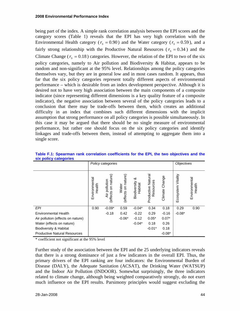
2008 Environmental Performance Index
28-Jan-2008 44
being part of the index. A simple rank correlation analysis between the EPI scores and the category scores (Table 1) reveals that the EPI has very high correlation with the Environmental Health category ( 90.0=Sr ) and the Water category ( 59.0=Sr ), and a fairly strong relationship with the Productive Natural Resources ( 34.0=Sr ) and the Climate Change ( 18.0=Sr ) categories. However, the relation of the EPI to two of the six policy categories, namely to Air pollution and Biodiversity & Habitat, appears to be random and non-significant at the 95% level. Relationships among the policy categories themselves vary, but they are in general low and in most cases random. It appears, thus far that the six policy categories represent totally different aspects of environmental performance – which is desirable from an index development perspective. Although it is desired not to have very high association between the main components of a composite indicator (since representing different dimensions is a key quality feature of a composite indicator), the negative association between several of the policy categories leads to a conclusion that there may be trade-offs between them, which creates an additional difficulty in an index that combines such different dimensions with the implicit assumption that strong performance on all policy categories is possible simultaneously. In this case it may be argued that there should be no single measure of environmental performance, but rather one should focus on the six policy categories and identify linkages and trade-offs between them, instead of attempting to aggregate them into a single score.
Table F.1: Spearman rank correlation coefficients for the EPI, the two objectives and the six policy categories Policy categories Objectives
Env
ironm
enta
l H
ealth
Air
pollu
tion
(effe
cts
on n
atur
e)
Wat
er
(effe
cts
on n
atur
e)
Bio
dive
rsity
&
Hab
itat
Pro
duct
ive
Nat
ural
R
esou
rces
Clim
ate
Cha
nge
Eco
syst
em V
italit
y
Env
ironm
enta
l H
ealth
EPI 0.90 -0.09* 0.59 -0.04* 0.34 0.18 0.29 0.90 Environmental Health -0.18 0.42 -0.22 0.29 -0.16 -0.08* Air pollution (effects on nature) -0.06* -0.12 0.05* 0.07* Water (effects on nature) -0.04* 0.18 0.26 Biodiversity & Habitat -0.01* 0.18 Productive Natural Resources -0.08*
* coefficient not significant at the 95% level Further study of the association between the EPI and the 25 underlying indicators reveals that there is a strong dominance of just a few indicators in the overall EPI. Thus, the primary drivers of the EPI ranking are four indicators: the Environmental Burden of Disease (DALY), the Adequate Sanitation (ACSAT), the Drinking Water (WATSUP) and the Indoor Air Pollution (INDOOR). Somewhat surprisingly, the three indicators related to climate change, although being weighted comparatively strongly, do not exert much influence on the EPI results. Parsimony principles would suggest excluding the

2008 Environmental Performance Index
28-Jan-2008 45
non-influential indicators from the EPI framework (Gall, 2007). This, however, may not be advisable from a policy perspective, unless excluding certain indicators is supported by expert opinion on the relevance of the indicators to the issue. An eventual revision of the EPI framework may be undertaken in terms of the weighting issue.
The scatter plot between the two main Objectives of the EPI, Environmental Health and Ecosystem Vitality, in Figure 1 points to an understandable - though problematic – trade-off between these two objectives. Countries may end up choosing one or the other path in pursuing environmental performance in a somewhat mutually exclusive pattern, perhaps descriptive of different scales and time horizons. This graph, therefore, points to a major problem in translating sustainability-oriented performance into practice. At the same time, the high association between the EPI scores and the Environmental Health scores, and the random association between the EPI scores and the Ecosystem Vitality scores leads to an Ecosystem’s performance behaving as a noise term superimposed to Environmental Health.
Figure 1. Scatterplot of the Environmental Health versus the Ecosystem Vitality scores
0
10
20
30
40
50
60
70
80
90
100
30 40 50 60 70 80 90 100
Ecosystem score
Envi
ronm
enta
l Hea
lth s
core
EPI rank 1-50EPI rank 51-100EPI rank 101-149
NorwaySweden Switzerland
Costa Rica
Sri Lanka
TajikistanNepal
Congo
Laos
Dem. Rep. Congo
Niger
Sierra Leone
Mavritania
Yemen
Djibouti
Solomon Islands
Iraq
United Arab Em.
KazakhstanKuwait
LebanonUkraine
Belgium USA Italy
India
The conclusions from this preliminary analysis already point to the conclusion that the 2008 EPI has an architecture that highlights the complexity of translating environmental stewardship into straightforward, clear-cut policy recipes. The trade-offs within the index dimensions are a reminder of the danger of compensability among the dimensions while identifying the areas where more work is needed to achieve a coherent framework in particular in terms of the relative importance of the indicators that compose the framework.

2008 Environmental Performance Index
28-Jan-2008 46
Robustness of the EPI results to the methodological assumptions There is ample evidence of the creativity in the community of composite indicators developers, which not only comes as a response to the demands of the user/stakeholder community, but it also reflects the disagreements within the research community on which indicators influence a particular phenomenon and on their relative importance (Cutter et al., 2003). When building an index to capture environmental performance, it is therefore necessary to take stock of existing methodologies to avoid skewing the assessment and decision-making.
By acknowledging a variety of methodological assumptions in the development of an index that are intrinsic to policy research, one can determine whether the main results change substantially when the assumptions are varied over a reasonable range of possibilities (Saisana et al., 2005; Saisana and Tarantola, 2002; Saltelli et al., 2000). The advantages offered by considering different scenarios to build the EPI could be: to gauge the robustness of the EPI results, to increase its transparency, to identify the countries whose performance improves or deteriorates under certain assumptions, and to help frame the debate around the use of the EPI for policy- making. The alternative scenarios to build the EPI should, however, bear certain quality features:
1. No strong dominance of a few indicators at the expense of others in the index. 2. No deliberate bias of the index results against a few countries. 3. Simplicity and easy reproduction of the index.
In the case of the 2008 EPI, the assumptions that needed to be tested, are: (1) the measurement error of the raw data, (2) the choice of capping the 25 indicators at the selected targets, (3) the choice to correct for skewed distributions in the indicator values, (4) the weights assigned to the indicators and/or to the subcomponents of the index, and finally (5) the aggregation function at the policy level. The analysis that we have undertaken maps the effects of these uncertainties and assumptions on the EPI country rankings. We also seek to use uncertainty and sensitivity analyses to assess whether useful conclusions can be drawn from the index given the construction methodology selected. Sensitivity analysis is the study of how output variation in models such as the EPI can be apportioned, qualitatively or quantitatively, to different sources of variation in the assumptions. In addition, it measures the extent to which the composite index depends upon the information that composes it. Sensitivity analysis is closely related to uncertainty analysis, which aims to quantify the overall variation in the ranking resulting from uncertainties in the model input. All of the five assumptions discussed above can heavily influence the output—and reliability—of the EPI. Using uncertainty and sensitivity analysis, we systematically evaluated the impact that the methodological and conceptual choices highlighted above have on the robustness of the EPI scoring and ranking. Our study aimed to answer four main questions.

2008 Environmental Performance Index
28-Jan-2008 47
1. What associations are there between the EPI and its indicators and/or subcomponents?
2. How do the EPI ranks compare to the ranks under combinations of alternative scenarios derived from the 5 assumptions?
3. Which countries have the most volatile ranks and why? 4. What are the major sources of variability in the EPI rankings?
The first question has already been discussed previously. Next, we will focus on the remaining three questions which call for a combined application of uncertainty and sensitivity analysis.
Our approach We focus on testing the five central methodological issues, which are translated into 40,000 simulations of different combinations of them. To be more specific, the measurement error is introduced by adding to each value in the dataset a random error with a mean equal to zero and standard deviation equal to the observed standard deviation of the corresponding indicator. Some thousands of alternative datasets that include error in some of the data values are generated. The two triggers on capping at target values and correcting for skewed data distributions are binary (yes/no). Regarding the weights to be attached to the indicators and/or the subcomponents, we have identified four alternatives to the current one: Factor analysis-derived weights at the indicator level; equal weighting at the indicator level; equal weighting at the subcategory level (and relative weights within each subcategory as in the EPI); equal weighting at the policy level (and relative weights within each policy category and subcategory as in the EPI). Finally, a binary trigger determines the aggregation function (at the policy level) to be an arithmetic or a geometric average. In the latter case, the use of a geometric aggregation would penalize countries that compensate very low performance in some policy categories with very high performance in other policy categories. Given that environmental excellence is understood to mean strong performance on the different EPI categories simultaneously, compensation at the policy level should be penalized. We undertook a saturated sampling of the space of input factors. The combinations of the input factors are translated into a set of N=40,000 simulations in a Monte Carlo framework. The composite index is then evaluated N times, and the EPI scores and ranks obtained are associated with the corresponding draws of input factors to appraise their influence. When several layers of uncertainty are simultaneously activated, composite indicators turn out to be non-linear, possibly non-additive models, due to interactions between the input factors (Saisana et al. 2005). As a result, all EPI scores and ranks are non-linear functions of the input factors and the purpose of the uncertainty analysis is the estimation of their probability distribution functions. As argued by practitioners (Saltelli et al., 2000b; EPA, 2004), robust, “model-free” techniques for sensitivity analysis should be used for non-linear models. Variance-based

2008 Environmental Performance Index
28-Jan-2008 48
techniques have been shown to yield useful results for sensitivity analysis. For more information the reader is referred elsewhere (e.g., Saltelli et al. 2008). 1. How do the EPI ranks compare to the ranks under all scenarios? The uncertainty analysis results from the Monte Carlo simulations for the 149 countries are given in detail in Table 2. They reveal whether any deliberate bias against some countries is introduced by making certain methodological choices in building the EPI and respond to arguments made by Andrews et al. (2004: 1323) that many indices “rarely have adequate scientific foundations to support precise rankings: […] typical practice is to acknowledge uncertainty in the text of the report and then to present a table with unambiguous rankings”. The countries shown in Table 2 are ordered by their original EPI score. The numbers in Table 2 represent the probability of a country being among the top 10, top 10-20, and so on. Just to give an example, New Zealand has a 98% probability to be among the top 10 performing countries. Costa Rica and Finland follow, with a probability of 81% to be ranked among the top 10. Interestingly, Switzerland, which scores top in the original EPI, is almost as likely to be among the top 10, top10-20 or top 20-30 countries. These probabilities indicate the uncertainty about the countries scores in the EPI. In fact, approximately half of the countries in the EPI are placed correctly in the environmental performance ladder, whilst the other half of the countries can fluctuate significantly between various positions, and any conclusion on the performance of these countries should be drawn with great caution. The results presented in Table 2 depend on the theoretical framework and the indicators, but are independent of the methodology (methodology-free results), given that they represent a whole set of alternative scenarios. The dominant source for the observed deviations arises from the choice of the weights and its combined effect with the choice of the aggregation function at the policy level. As Table 2 demonstrates, countries with high or low performance in the EPI do not have wide variations in their ranks under alternative scenarios. The exceptions to this rule are Austria, Canada, and Iceland. In our simulations Austria ranked between the top 10 to the top 40-50. Another interesting example is Iceland (rank: 11) whose score can be anywhere within the top10-20 to top 80-90. Canada, on the other hand (rank: 12) has a 58% probability to be ranked in the top10 and 33% to be ranked among the top10-20. This result suggests that in fact Canada outperforms Iceland on the environmental issues measured in the EPI given the current framework.

2008 Environmental Performance Index
28-Jan-2008 49
Which countries have the most volatile ranks and why?
Ran
k 1-
10
Ran
k 11
-20
Ran
k 21
-30
Ran
k 31
-40
Ran
k 41
-50
Ran
k 51
-60
Ran
k 61
-70
Ran
k 71
-80
Ran
k 81
-90
Ran
k 91
-100
Ran
k 10
1-11
0
Ran
k 11
1-12
0
Ran
k 12
1-13
0
Ran
k 13
1-14
0
Ran
k 14
1-14
9
Viet Nam 0 1 1 5 10 18 29 20 8 4 4 1 0 0 0Nicaragua 1 1 8 21 28 14 10 14 4 0 0 0 0 0 0S audi Arabia 0 1 1 1 1 11 13 23 16 10 11 4 4 4 0Tajikis tan 0 0 0 0 3 3 9 6 14 19 18 19 11 0 0Azerbaijan 0 0 0 0 0 1 0 3 10 23 9 24 26 5 0Nepal 0 0 1 1 5 9 8 15 28 14 13 6 1 0 0Morocco 0 0 0 0 1 0 1 14 20 15 13 15 16 3 3R omania 0 0 3 3 1 14 10 33 16 11 3 5 3 0 0Belize 0 4 9 29 16 13 4 14 6 3 0 4 0 0 0Turkmenis tan 0 0 0 1 5 6 14 8 19 25 11 9 3 0 0Ghana 4 11 14 16 10 10 13 9 8 5 1 0 0 0 0Moldova 0 0 0 0 0 0 0 1 4 8 4 10 13 30 31Namibia 0 0 0 1 4 1 16 16 25 18 16 3 0 0 0T rinidad & To 0 1 4 6 20 11 23 8 13 8 3 5 0 0 0Lebanon 0 0 0 0 0 5 15 13 13 5 5 6 20 8 11Oman 0 0 0 1 1 10 25 18 24 5 10 4 1 1 0F iji 0 0 0 0 0 1 4 4 6 15 13 19 14 20 5C ongo 0 0 3 9 1 23 18 13 13 13 9 1 0 0 0K yrgyzs tan 0 0 0 1 1 5 6 15 13 30 15 9 4 1 0Z imbabwe 0 0 4 4 21 11 15 10 15 13 6 0 1 0 0Kenya 1 18 15 11 11 11 11 6 8 6 1 0 0 0 0S outh Africa 0 1 4 3 14 16 20 11 16 11 1 3 0 0 0Botswana 0 0 0 0 0 5 1 3 13 18 18 19 16 6 3S yria 0 0 0 0 0 0 0 0 3 16 11 21 13 30 6Mongolia 0 0 3 5 0 13 9 25 18 15 10 4 0 0 0L aos 1 3 3 10 8 9 10 6 10 9 19 11 3 0 0Indones ia 0 0 3 9 10 11 23 19 14 5 6 0 1 0 0C ôte d'Ivoire 1 4 10 13 15 20 8 11 3 9 6 0 1 0 0Myanmar 0 0 0 0 0 3 6 5 16 24 26 15 5 0 0C hina 0 0 0 1 3 3 9 13 9 25 19 13 5 1 1Uzbekis tan 0 0 0 0 0 0 0 0 0 1 14 16 29 29 11K azakhstan 0 0 0 0 0 0 0 0 1 5 15 16 36 24 3Guyana 0 0 0 0 3 6 10 19 15 20 20 5 3 0 0P apua New G 0 0 0 0 1 6 10 14 9 11 20 20 8 0 1Bolivia 0 0 0 0 4 4 8 10 23 13 20 11 4 4 1Kuwait 0 0 0 0 0 0 0 1 0 1 9 5 15 28 41United Arab E 0 0 0 0 0 0 0 0 4 10 9 36 19 11 11Tanzania 1 3 4 11 13 16 9 11 11 8 6 6 1 0 0C ameroon 0 0 3 0 1 6 10 6 13 23 23 15 1 0 0S enegal 0 0 0 0 3 5 6 9 16 30 24 6 1 0 0Togo 0 0 0 1 0 3 8 6 18 18 18 18 10 3 0Uganda 0 0 0 0 3 8 5 5 6 11 20 21 11 10 0S waziland 0 0 0 0 0 0 0 1 6 4 16 31 24 15 3Haiti 0 0 0 0 0 0 1 1 1 3 10 21 23 30 10India 0 0 0 0 0 0 0 3 0 11 15 31 25 13 3Malawi 0 1 0 0 9 13 13 14 3 11 15 9 6 8 0E ritrea 0 0 0 0 1 1 1 6 13 16 16 25 18 3 0E thiopia 0 0 0 0 1 1 3 6 8 9 8 9 25 26 5P akis tan 0 0 0 0 0 3 0 3 23 9 26 18 18 1 1Bangladesh 0 0 0 0 0 0 0 0 0 1 1 9 18 24 48Nigeria 0 0 0 1 1 0 1 6 5 13 15 24 23 6 5Benin 0 0 0 1 4 10 11 10 14 13 9 11 13 3 3C entral Afr. R 0 0 0 0 0 0 0 1 4 3 13 14 16 38 13S udan 0 0 0 0 0 0 0 1 0 1 1 10 34 46 6Z ambia 0 0 0 0 0 1 0 3 10 10 14 9 21 21 11Rwanda 0 0 1 0 6 3 11 18 11 18 5 13 6 9 0Burundi 0 0 0 0 0 0 3 9 8 15 9 18 29 11 0Madagascar 0 0 0 0 0 1 3 3 8 13 16 20 21 15 1Mozambique 0 0 0 0 1 1 6 6 9 11 14 18 21 9 4Iraq 0 0 0 0 0 0 0 0 0 0 0 3 11 26 60C ambodia 0 0 0 0 0 0 0 0 4 8 15 11 31 28 4S olomon Is lan 0 0 0 0 0 0 0 0 0 0 0 0 3 16 81Guinea 0 0 0 0 0 0 0 3 3 4 13 14 23 36 6Djibouti 0 0 0 0 0 0 0 0 0 0 1 8 18 35 39Guinea‐B issa 0 0 0 0 0 0 1 0 4 15 14 28 19 15 5Y emen 0 0 0 0 0 0 0 0 0 0 0 3 6 29 63Dem. R ep. C o 0 0 0 0 0 1 0 1 3 4 1 13 29 26 23C had 0 0 0 0 0 0 0 0 0 0 4 8 16 33 40Burkina F aso 0 0 0 0 0 0 0 0 0 0 9 6 18 43 25Mali 0 0 0 0 0 0 0 0 0 0 0 5 18 36 41Mauritania 0 0 0 0 0 0 0 0 0 3 0 9 25 40 24S ierra Leone 0 0 0 0 0 0 0 0 0 0 0 1 11 18 70Angola 0 0 0 0 0 0 0 0 0 0 0 0 3 19 79Niger 0 0 0 0 0 0 0 0 0 0 0 3 6 19 73
Ran
k 1-
10
Ran
k 11
-20
Ran
k 21
-30
Ran
k 31
-40
Ran
k 41
-50
Ran
k 51
-60
Ran
k 61
-70
Ran
k 71
-80
Ran
k 81
-90
Ran
k 91
-100
Ran
k 10
1-11
0
Ran
k 11
1-12
0
Ran
k 12
1-13
0
Ran
k 13
1-14
0
Ran
k 14
1-14
9
S witzerland 31 30 20 11 6 1 0 0 0 0 0 0 0 0 0S weden 63 25 10 1 1 0 0 0 0 0 0 0 0 0 0Norway 55 31 6 3 3 3 0 0 0 0 0 0 0 0 0F inland 81 16 0 0 3 0 0 0 0 0 0 0 0 0 0C osta R ica 81 16 0 1 0 1 0 0 0 0 0 0 0 0 0Austria 15 19 16 21 18 4 4 1 0 3 0 0 0 0 0New Z ealand 98 1 0 1 0 0 0 0 0 0 0 0 0 0 0Latvia 25 39 26 6 4 0 0 0 0 0 0 0 0 0 0C olombia 74 18 5 1 3 0 0 0 0 0 0 0 0 0 0F rance 15 26 30 14 13 1 0 0 0 0 0 1 0 0 0Iceland 3 11 15 5 14 15 9 10 13 3 4 0 0 0 0C anada 58 33 9 1 0 0 0 0 0 0 0 0 0 0 0Germany 1 14 40 21 20 4 0 0 0 0 0 0 0 0 0United K ingdo 11 44 29 11 4 1 0 0 0 0 0 0 0 0 0S lovenia 1 9 18 25 23 8 10 1 4 1 1 0 0 0 0L ithuania 3 16 20 14 9 8 9 6 9 3 1 0 3 1 0S lovakia 0 15 21 4 14 25 5 6 8 1 1 0 0 0 0Portugal 20 46 16 11 5 1 0 0 0 0 0 0 0 0 0E s tonia 56 34 4 3 0 1 3 0 0 0 0 0 0 0 0C roatia 3 16 19 23 10 6 9 5 5 5 0 0 0 0 0J apan 6 38 35 14 5 1 1 0 0 0 0 0 0 0 0E cuador 63 26 3 5 4 0 0 0 0 0 0 0 0 0 0Hungary 0 4 1 6 1 6 13 16 20 4 6 10 9 4 0Italy 1 6 28 24 16 13 5 4 4 0 0 0 0 0 0Denmark 1 1 8 3 9 6 15 13 14 8 6 11 0 4 3Malays ia 31 48 15 5 1 0 0 0 0 0 0 0 0 0 0Albania 0 3 9 11 6 13 10 16 3 5 6 4 9 5 1R uss ia 9 33 43 9 4 3 1 0 0 0 0 0 0 0 0C hile 16 46 25 8 1 1 3 0 0 0 0 0 0 0 0S pain 0 5 30 18 19 14 11 3 0 0 1 0 0 0 0Luxembourg 0 9 3 15 16 20 26 5 5 1 0 0 0 0 0P anama 73 20 4 3 0 1 0 0 0 0 0 0 0 0 0Dominican R e 18 54 21 6 0 0 1 0 0 0 0 0 0 0 0Ireland 1 4 5 16 13 15 13 13 4 1 9 5 3 0 0Brazil 5 20 29 24 11 4 3 4 0 0 0 1 0 0 0Uruguay 0 3 3 11 15 9 8 9 10 3 9 4 4 14 1Georgia 0 1 1 8 8 19 15 16 10 13 5 1 1 1 1Argentina 0 1 10 23 28 24 11 1 3 0 0 0 0 0 0United S tates 5 23 19 24 13 8 4 3 3 0 1 0 0 0 0Taiwan 0 1 3 20 13 19 16 10 13 4 1 1 0 0 0C uba 3 5 24 29 19 13 5 4 0 0 0 0 0 0 0Poland 4 5 11 20 35 15 3 3 3 1 0 0 1 0 0Belarus 0 0 0 1 11 10 10 18 16 16 13 3 0 1 1Greece 1 0 4 8 18 14 19 15 0 5 10 6 0 1 0Venezuela 5 11 36 25 18 5 0 0 0 0 0 0 0 0 0Australia 30 30 14 10 9 3 3 1 1 0 0 0 0 0 0Mexico 1 11 15 34 28 3 6 1 1 0 0 0 0 0 0Bosnia & Herz 0 0 1 0 5 4 10 11 24 9 6 8 3 14 6Is rael 0 0 1 5 31 19 19 13 5 6 1 0 0 0 0S ri Lanka 19 36 16 16 10 3 0 0 0 0 0 0 0 0 0S outh Korea 0 1 1 3 6 3 14 14 19 9 8 13 8 1 3C yprus 0 1 0 10 9 25 14 28 6 4 1 3 0 0 0Thailand 0 8 30 35 11 11 1 1 3 0 0 0 0 0 0J amaica 0 0 4 8 15 24 11 11 9 10 5 1 3 0 0Netherlands 0 0 3 3 0 9 11 14 10 21 9 11 9 0 1Bulgaria 0 1 3 5 19 25 15 8 10 6 4 4 1 0 0Belgium 0 0 3 3 1 13 6 11 6 6 16 10 13 9 4Mauritius 0 0 1 4 6 9 19 18 8 16 15 3 3 0 0Tunis ia 0 0 0 0 1 5 10 10 10 14 19 18 9 4 1P eru 0 3 15 30 18 30 4 0 0 1 0 0 0 0 0Philippines 1 6 13 26 21 16 9 3 5 0 0 0 0 0 0Armenia 0 0 1 0 3 3 6 13 19 8 16 18 8 6 1P araguay 0 0 0 4 11 18 20 18 9 8 5 6 3 0 0Gabon 0 6 35 28 16 5 6 3 1 0 0 0 0 0 0E l S alvador 0 0 5 6 4 13 16 9 10 9 8 9 8 5 0Algeria 0 0 5 5 15 26 24 11 6 5 3 0 0 0 0Iran 1 3 11 23 26 18 16 1 1 0 0 0 0 0 0C zech R ep. 0 0 0 0 0 9 8 15 11 13 19 15 10 0 1Guatemala 0 10 16 23 26 14 8 3 1 0 0 0 0 0 0J ordan 0 0 1 3 0 8 14 24 20 6 14 8 1 1 1E gypt 0 3 19 21 24 13 10 6 3 0 3 0 0 0 0Turkey 0 0 0 1 3 4 18 15 18 16 9 6 6 4 1Honduras 4 9 28 20 15 13 8 5 0 0 0 0 0 0 0Macedonia 0 0 0 1 1 5 5 15 10 18 21 13 6 5 0Ukraine 0 0 0 0 0 4 8 15 6 23 11 10 13 10 1
Table 2. Probabilities of country ranks in the Environmental Performance Index under all tested combinations of input factors (probabilities less than 5% are not shown)

2008 Environmental Performance Index
28-Jan-2008 50
We use the term “volatility” as a measure of the difference between a country’s best and worst rank, calculated from the 5th and the 95th percentiles of the rank distribution simulations. For Finland, Costa Rica, New Zealand, Colombia and Panama, we can reasonably state that they have a top 10 performance (probability greater than 70%) and very low volatility in their scores. Interestingly, Panama is ranked 32nd in the EPI – a rank that occurs less than 5% of the times in our simulations. Table 3 presents the 20 countries that are affected most strongly by the methodological choices made during the construction of the EPI. These countries, with a difference in their best and worst rank (5th and 95th percentiles) of at least 80 positions, are ranked between 11th (Iceland) and 131st (Rwanda). A number of those countries such as Lithuania, Hungary, Denmark, Albania, Ireland, Uruguay, and Bosnia & Herzegovina are ranked among the top 50 in the EPI. The volatility of those countries’ ranks can be attributed mainly to the choice of the weighting combined with the aggregation scheme at the policy level. Table 3. Most volatile countries in the EPI Country
EPI Rank
Range of Simulation Ranks
Country EPI Rank
Range of Simulation Ranks
Iceland 11 [14,95] El Salvador 65 [31,129] Lithuania 16 [16,98] Ghana 86 [12,93] Hungary 23 [33,129] Lebanon 89 [62,143] Denmark 25 [25,131] Kenya 96 [13,98] Albania 27 [25,132] Laos 101 [29,116] Ireland 34 [24,114] Côte d'Ivoire 103 [21,103] Uruguay 36 [31,139] Tanzania 113 [23,113] Bosnia & Herzegovina
48 [48,141] Uganda 117 [55,134]
South Korea 51 [42,125] Malawi 121 [48,132] Belgium 57 [42,137] Benin 127 [51,130] Rwanda 131 [45,131]
3. What are the sources of major impact on the variability of the EPI ranking? We now focus on assessing the impact of each of the five assumptions individually, which amounts to a total of eight different scenarios. We undertake the following comparisons:
Measurement error • current case without measurement error in the data vs. measurement error in the data;
Winsorisation • current winsorisation approach vs. no winorisation;
Target values • current target values v. no target values;
Weighting • current weighting vs. FA-derived weights at the indicator level;

2008 Environmental Performance Index
28-Jan-2008 51
• current weighting vs. equal weighting at the indicator level; • current weighting vs. equal weighting at the subcategory level; • current weighting vs. equal weighting at the policy level;
Aggregation • current arithmetic aggregation vs. geometric aggregation at the policy level.
Measurement error It is reasonable to assume that the raw data are not flawless and that despite efforts to guarantee the most reliable sources for them, errors may still be present. To account for this, we have added a normally distributed random error term to the raw data with a mean zero and a standard deviation equal to the observed one for each indicator. Table 4 presents the countries that are mostly affected by this assumption. Most notably, Luxembourg (rank: 31) would deteriorate its rank by 53 positions. On the other extreme, the Philippines (rank: 61) would improve its rank and be placed in the 10th position. Overall, the introduction of measurement error in the raw data has a median impact of 9 ranks and a 90th percentile impact of 29 positions. In other words, this assumptions leaves 1 out of 2 countries almost unaffected (less than 9 positions change), but 1 out of 10 countries would shift more than 29 positions. Table 4: Countries most affected by measurement error compared to the original EPI. EPI rank Rank Difference Top five countries Colombia 9 42 -33 Costa Rica Iceland 11 47 -36 Dominican Rep. Estonia 19 60 -41 Norway Luxembourg 31 84 -53 Finland Dominican Rep. 33 2 31 Canada Cuba 41 74 -33 Poland 42 83 -41 Bottom five countries South Korea 51 18 33 Cambodia Peru 60 27 33 Mauritania Philippines 61 10 51 Angola Iran 67 32 35 Burkina Faso Honduras 73 38 35 Sierra Leone Nepal 81 115 -34 Fiji 94 54 40 Median change: 9 ranks South Africa 97 57 40 90th percentile change: 29 ranks
Winsorization Winsorization is also expected to have an impact on the rankings, particularly for those countries that present a few extreme values. Table 5 presents the countries that are mostly affected by the choice of not winsorizing, as opposed to the current one. In the best case,

2008 Environmental Performance Index
28-Jan-2008 52
South Africa (rank: 97) improves its position by 16, whilst in the worst case, Botswana (rank: 98) declines by 21 ranks. For 1 out of 2 countries, the impact of this assumption is only 5 positions, while 1 out of 10 countries shift by more than 11 positions, but not more than 21. Table 5: Countries most affected by not winsorizing skewed distributions compared to the original EPI. EPI rank Rank Difference Top five countries Hungary 23 39 -16 Sweden Luxembourg 31 48 -17 Norway Georgia 37 50 -13 Switzerland Belarus 43 56 -13 New Zealand Bosnia & Herzegovina 48 61 -13 Costa Rica Tajikistan 79 95 -16 Azerbaijan 80 96 -16 Bottom five countries Lebanon 89 75 14 Mali Fiji 94 107 -13 Chad South Africa 97 81 16 Sierra Leone Botswana 98 119 -21 Niger Indonesia 102 87 15 Angola Côte d'Ivoire 103 91 12 Uzbekistan 106 125 -19 Median change: 5 ranks Tanzania 113 99 14 90th percentile change: 11
ranks
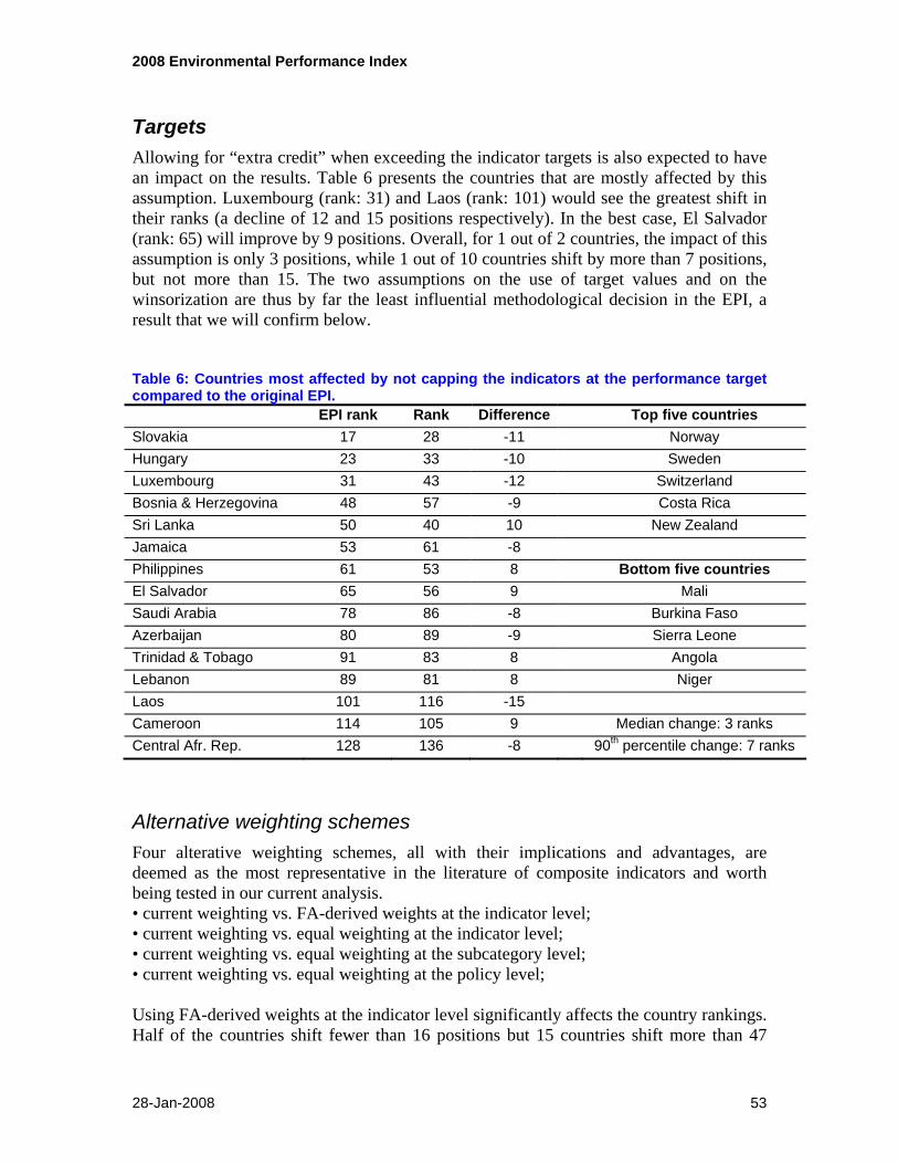
2008 Environmental Performance Index
28-Jan-2008 53
Targets Allowing for “extra credit” when exceeding the indicator targets is also expected to have an impact on the results. Table 6 presents the countries that are mostly affected by this assumption. Luxembourg (rank: 31) and Laos (rank: 101) would see the greatest shift in their ranks (a decline of 12 and 15 positions respectively). In the best case, El Salvador (rank: 65) will improve by 9 positions. Overall, for 1 out of 2 countries, the impact of this assumption is only 3 positions, while 1 out of 10 countries shift by more than 7 positions, but not more than 15. The two assumptions on the use of target values and on the winsorization are thus by far the least influential methodological decision in the EPI, a result that we will confirm below. Table 6: Countries most affected by not capping the indicators at the performance target compared to the original EPI. EPI rank Rank Difference Top five countries Slovakia 17 28 -11 Norway Hungary 23 33 -10 Sweden Luxembourg 31 43 -12 Switzerland Bosnia & Herzegovina 48 57 -9 Costa Rica Sri Lanka 50 40 10 New Zealand Jamaica 53 61 -8 Philippines 61 53 8 Bottom five countries El Salvador 65 56 9 Mali Saudi Arabia 78 86 -8 Burkina Faso Azerbaijan 80 89 -9 Sierra Leone Trinidad & Tobago 91 83 8 Angola Lebanon 89 81 8 Niger Laos 101 116 -15 Cameroon 114 105 9 Median change: 3 ranks Central Afr. Rep. 128 136 -8 90th percentile change: 7 ranks
Alternative weighting schemes Four alterative weighting schemes, all with their implications and advantages, are deemed as the most representative in the literature of composite indicators and worth being tested in our current analysis. • current weighting vs. FA-derived weights at the indicator level; • current weighting vs. equal weighting at the indicator level; • current weighting vs. equal weighting at the subcategory level; • current weighting vs. equal weighting at the policy level; Using FA-derived weights at the indicator level significantly affects the country rankings. Half of the countries shift fewer than 16 positions but 15 countries shift more than 47

2008 Environmental Performance Index
28-Jan-2008 54
positions. Table 7 shows the countries that experience the biggest shift in their rank due to this assumption. Table 7: Countries most affected by the FA weights compared to the original EPI. EPI rank Rank Difference Top five countries Lithuania 16 63 -47 Switzerland Hungary 23 75 -52 Finland Denmark 25 79 -54 New Zealand Albania 27 93 -66 Estonia Georgia 37 87 -50 Austria Bosnia & Herzegovina 48 99 -51 South Korea 51 105 -54 Bottom five countries Egypt 71 23 48 Angola Saudi Arabia 78 17 61 Yemen Belize 84 21 63 Bangladesh Moldova 87 134 -47 Solomon Islands Trinidad & Tobago 91 40 51 Sierra Leone Zimbabwe 95 48 47 Kenya 96 45 51 Median change: 16 ranks Mongolia 100 33 67 90th percentile change: 47 ranks
Equal weighting at the indicator level would increase the weight of the indicators in the Air Pollution (effects on nature) subcategory, the Water (effects on nature), the Biodiversity and Habitat category, and the Productive Natural Resources category. A total of seventeen indicators will increase their weight, as opposed to the current weighting scheme. The remaining eight indicators will reduce their weight, in particular, the DALY indicator and the three indicators related to Climate Change. The countries whose EPI ranks are most affected by this change are shown in Table 8. The countries that improve their ranks the most are Laos, Kenya, Mongolia and Malawi (by more than 60 positions upwards). On the other hand, Denmark and South Korea decline more than 70 positions. Overall, for 1 out of 2 countries, the impact of this assumption is 15 positions, while 1 out of 10 countries shift by more than 48 positions (up to 72 positions). Table 8: Countries most affected by using equal weights at the indicator level compared to the original EPI. EPI rank Rank Difference Top five countries Hungary 23 80 -57 Switzerland Denmark 25 97 -72 Finland South Korea 51 122 -71 New Zealand Belgium 57 115 -58 Estonia Tunisia 59 117 -58 Colombia Ukraine 75 124 -49 Belize 84 35 49 Bottom five countries Moldova 87 139 -52 Yemen

2008 Environmental Performance Index
28-Jan-2008 55
Congo 92 39 53 Angola Kenya 96 29 67 Iraq Mongolia 100 33 67 Bangladesh Laos 101 17 84 Solomon Islands Côte d'Ivoire 103 49 54 Malawi 121 55 66 Median change: 15 ranks Rwanda 131 77 54 90th percentile change: 48 ranks
We next tested the impact of an equal weighting at the subcategory level, whilst the relative weights for the indicators within each subcategory remain as in the EPI. This is expected to have a less pronounced impact on the EPI ranks because this assumption assigns greater weight to the six of the ten subcategories and reduces the weight of the other four and in particular the weight of the climate change and of the environmental burden of disease (DALY). As a consequence, the countries whose EPI ranks are most affected by this change are given in Table 9. The countries that improve their ranks the most are Trinidad & Tobago and Laos (improvement of more than 38 positions). On the other hand, Denmark and Taiwan decline more than 50 positions. Overall, for 1 out of 2 countries, the impact of this assumption is 9 positions, while 1 out of 10 countries shift by more than 26 positions (up to 51 positions). Table 9: Countries most affected by equal weighting at the subcategory level compared to the original EPI. EPI rank Rank Difference Top five countries Denmark 25 76 -51 Switzerland Argentina 38 65 -27 Finland Taiwan 40 90 -50 New Zealand Australia 46 18 28 Sweden South Korea 51 100 -49 Colombia Netherlands 54 86 -32 Belgium 57 101 -44 Bottom five countries Mauritius 58 29 29 Dem. Rep. Congo Tunisia 59 92 -33 Niger Gabon 64 37 27 Bangladesh Belize 84 49 35 Angola Trinidad & Tobago 91 50 41 Mauritania Fiji 94 66 28 Mongolia 100 72 28 Median change: 9 ranks Laos 101 63 38 90th percentile change: 26
ranks We conclude the assessment of the impact of different weighting methods by evaluating the impact of equal weighting at the policy level. The relative weights within the policy categories and within the subcategories remain the same as in the EPI. A weight of 1/6 is

2008 Environmental Performance Index
28-Jan-2008 56
thus assigned to each policy category, thus reducing significantly the previously assigned weight of .50 to the environmental health and the weight of 0.25 assigned original to climate change. All policy categories now have a weight of 1/6 = .167. The countries whose EPI ranks are most affected by this change are given in Table 10. The countries with the most notable improvement in their ranks are Laos and Kenya (improvement of more than 78 positions). On the other hand, Belgium and South Korea decline more than 75 positions. Overall, for 1 out of 2 countries, the impact of this assumption is 18 positions, while 1 out of 10 countries shift by more than 486 positions (up to 91 positions). Table 10: Countries most affected by equal weighting at the policy category level compared to the original EPI. EPI rank Rank Difference Top five countries Denmark 25 77 -52 Switzerland United States 39 87 -48 Finland Taiwan 40 101 -61 Sweden South Korea 51 126 -75 Norway Netherlands 54 122 -68 New Zealand Belgium 57 138 -81 Tunisia 59 111 -52 Bottom five countries Armenia 62 110 -48 Solomon Islands Ukraine 75 123 -48 Djibouti Belize 84 30 54 Yemen Lebanon 89 137 -48 Iraq Congo 92 23 69 Kuwait Kenya 96 18 78 Mongolia 100 35 65 Median change: 18 ranks Laos 101 10 91 90th percentile change: 48
ranks
Aggregation scheme at the policy level We assume that compensability is allowed among the indicators within each policy category but not desirable across the policy categories, consistently with the current theories that environmental aspects should be non compensatory. Table 11 presents those countries for which the most notable shift in the country rank occurs when a non-compensatory aggregation is performed at the policy level, i.e., a geometric mean function instead of an arithmetic mean function. Sri Lanka, Peru and Egypt improve their ranks by 18 positions or more, whilst the most decline is observed for Uruguay (down more than 51 positions). Overall, for 1 out of 2 countries, the impact of this assumption is merely 5 positions, while 1 out of 10 countries shift by more than 18 positions (up to 51 positions).

2008 Environmental Performance Index
28-Jan-2008 57
Table 11: Countries most affected by geometric aggregation at the policy level compared to the original EPI. EPI rank Rank Difference Top five countries Hungary 23 45 -22 Switzerland Albania 27 62 -35 Norway Ireland 34 58 -24 Sweden Uruguay 36 87 -51 Finland Greece 44 66 -22 Costa Rica Bosnia & Herzegovina 48 94 -46 Sri Lanka 50 31 19 Bottom five countries Peru 60 42 18 Dem. Rep. Congo El Salvador 65 83 -18 Mali Egypt 71 51 20 Sierra Leone Turkey 72 91 -19 Angola Ukraine 75 96 -21 Niger Moldova 87 113 -26 Lebanon 89 119 -30 Median change: 5 ranks Kazakhstan 107 126 -19 90th percentile change: 18 ranks
As expected and confirmed in all cases discussed above, middle-of-the-road performers display higher variability than the top and bottom countries. Summing up, when only one input factor is changed at a time, the most significant impact to the EPI ranking is attributable to the weighting method, in particular when choosing equal weights at the policy level (and original weights within each policy) compared to the original EPI, equally weighting all indicators, or using factor analysis derived weights at the indicators level. In any of these three cases, 1 out of 2 countries shifts less than 15 positions with respect to the original EPI ranking, whilst 1 out of 10 countries shifts more than 50 positions. The addition of measurement error and the impact of an equal weighting at the subcategories also have significant impact on the EPI ranking (1 out of 2 countries shifts less than 9 positions, but 1 out of 10 countries shift close to 30 positions or more). The least influential input factor is the decision on whether to cap performance at the indicator targets and winsorisation. In fact, 1 out of 2 countries shift less than five positions in the overall ranking and 1 out of 10 countries shift more than 10 positions, but not more than 21 positions.

2008 Environmental Performance Index
28-Jan-2008 58
Figure 2. Sensitivity analysis: impact of one-at-a-time changes in the five tested assumptions on the EPI ranking.
Note: median versus 90th percentile of the absolute differences in the rank score between a given scenario and the EPI. EW stands for equal weighting. When all sources of uncertainty are allowed to vary simultaneously their combined effect becomes even more important. The use of geometric aggregation combined with equal weighting at the policy level, with/without targets, without winsorization, and without measurement error affects half of the countries by more than 39 positions, of which 1 out of 10 is affected by a median shift of 69 positions. The main graph which we propose as representative of the environmental performance of the countries world-wide, given the current framework, but free of methodological choices (since these choices have already been summarized by the different scenarios) shows the probabilities that a country is ranked in the 1-10 position, or 11-20, etc. (Table 2).
EPI and Variability Countries that are situated in the top or mid-way in the EPI ranking tend to score uniformly high on the various indicators. In other words, these countries display a relatively low variability, which equals the coefficient of variation across the 25 indicators values for a given country. Figure 3 shows that the variability increases further down the EPI ranking. This scissors pattern is evident, and pronounced. The correlation coefficient between the EPI and the coefficient of variation series is equal to 78.0−=r , indicating a fairly high degree of reverse association between the EPI scores and the variability in the underlying indicators. For comparison purposes, in the case of the Trade and Development Index (UNCTAD, 2005) that is based on eleven components and
0
10
20
30
40
50
60
0 2 4 6 8 10 12 14 16 18 20
median
90th
per
cent
ile
EW subcategories
EW all indicators EW policies
FA all indicators
Geometric aggregation at the policy level
Without winsorisation
Without targets
With measurement error

2008 Environmental Performance Index
28-Jan-2008 59
developed for 110 countries, the correlation coefficient between the index scores and the coefficients of variation series was much higher and equal to 93.0−=r .
Figure 3. The scissor diagram of EPI and variability
0
20
40
60
80
100
120
2008
EPI
Sco
re
0.0
0.1
0.2
0.3
0.4
0.5
0.6
0.7
0.8
0.9
1.0
Coe
ffici
ent o
f var
iatio
n
EPI Variability
An implication of this finding is that while changes in the EPI scores over time could be regarded as a quantitative indication of trends in environmental performance, those with respect to the variability of the ranks could be seen as qualitative changes. Reducing even further the variability in the indicators should be among the objectives of environmental policies and strategies. To be successful, a country must put simultaneously invest in multiple goals within a coherent environmental performance strategy, while emphasizing reduction of the existing gaps in areas where performance is lagging. By demonstrating significant inter-country differences in the values of the coefficient of variation, the scissors diagram (Figure 3) points to the importance of country-specific approaches to environmental strategies. At the same time, though, it is unlikely that these variations will be reduced without coherent environmental policies and decision-making.
Concluding remarks The methodological approach used to construct the 2008 EPI was studied in this section. The “statistical” filters of index quality show that, although the theoretical framework and the indicators were carefully chosen by experts, the issue of weighting is crucial to obtain a robust performance index. The current weighting scheme results in an EPI that is dominated by very few indicators while having an almost random association with several other underlying indicators. With respect to the five input factors tested in the
2008 Environmental Performance Index
28-Jan-2008 60
sensitivity and uncertainty analysis, the country rankings are relatively reliable for approximately half of the countries, while any conclusion on the ranking for the other half of the countries should be made with great caution. An equal weighting approach at the indicator level, or at the policy level, as opposed to the current weighting scheme greatly influences the ranks. Thus, the choice of the weights must be evaluated according to its analytical rationale, policy relevance, and implied value judgments. The real value of the EPI lies not in the overall ranking of the countries, but rather in the solid framework and construction of the indicators. It is from this perspective that further revision of the index should be considered if the goal is to arrive at a single number that provides meaningful input to policy-making.
2008 Environmental Performance Index
28-Jan-2008 61
APPENDIX E: INDICATOR METADATA

2008 Environmental Performance Index
28-Jan-2008 62

EPI2008 Variables Metadata
Indicator 1: Environmental Burden of Disease
Indicator 2: Adequate Sanitation
Indicator 3: Drinking Water
Indicator 4: Urban Particulates
Indicator 5: Indoor Air Pollution
Indicator 6: Local Ozone
Indicator 7: Regional Ozone
Indicator 8: Sulfur Dioxide (SO2) emissions
Indicator 9: Water Quality Index
Indicator 10: Water Stress
Indicator 11: Conservation Risk Index
Indicator 12: Effective Conservation
Indicator 13: Critical Habitat Protection
Indicator 14: Marine Protected Areas
Indicator 15: Change in Growing Stock
Indicator 16: Marine Trophic Index
Indicator 17: Trawling Intensity
Indicator 18: Irrigation Stress
Indicator 19: Agricultural Subsidies
Indicator 20: Intensive Cropland
Indicator 21: Pesticide Regulation
Indicator 22: Burned Area
Indicator 23: Emissions Per Capita
Indicator 24: CO2 from Electricity Production
Indicator 25: Industrial Carbon Intensity

Indicator Code: DALY Objective: Environmental Health Policy Category: Environmental Health Subcategory: Environmental Burden of Disease Indicator Short Name: Environmental Burden of Disease Indicator Full Name: Disability Adjusted Life Years (DALY) Due to the Environmental Burden of Disease Indicator Description: The Disability Adjusted Life Year or DALY is a health gap measure that extends the concept of potential years of life lost due to premature death (PYLL) to include equivalent years of ‘healthy’ life lost by virtue of being in states of poor health or disability (Murray et al. 2002). The DALY combines in one measure the time lived with disability and the time lost due to premature mortality. One DALY can be thought of as one lost year of ‘healthy’ life and the burden of disease as a measurement of the gap between current health status and an ideal situation where everyone lives into old age free of disease and disability (WHO 2007). The WHO also captures environmental impact on human health through the DALY. These DALYs adjust the nominal deaths due to given, environmentally related diseases to take into account the years of life lost due to premature mortality and the loss in quality of life due to disability (morbidity). They are the sum of the number of life years lost due to premature mortality on account of an environmentally influenced disease and the years of life due to disability caused by that disease. Units: Years of life lost per 1,000 population Country Coverage: 192 Reference Year: 2002 Target: 0 Target Source: Expert judgment Short Source: WHO 2007 Source: WHO (World Health Organization). 2007, Country Profiles of Environmental Burden of Disease, Available online at http://www.who.int/quantifying_ehimpacts/countryprofiles/en/index.html. This report draws on WHO/UNICEF (2006). Taiwan: Department of Environmental Monitoring and Information Management, EPA. Source URL: http://www.who.int/quantifying_ehimpacts/countryprofiles/en/index.html
Methodology: The complete methodology for calculating DALYs is described in the source publication. The DALY indicator used by the 2008 EPI is an aggregate of DALY data that has been collected by the WHO. In order to represent Environmental Health across a broad spectrum of risks, the 2008 EPI does not limit its inquiry to one source of risk. Instead, the DALY indicator is an un‐weighted aggregate sum of DALY data from three sources of environmental health risk: diarrhea (due to inadequate sanitation and unclean drinking water), indoor air (combustion of solid fuels for household use), and outdoor air (concentration of particulate matter in urban areas). Twenty three countries had missing diarrhea data; these were mostly wealthy countries for which it made sense to assume relatively low levels of diarrhea. We analyzed the relationship between per‐capita income and diarrhea, and imputed missing values according to the following table: Per‐capita income* Imputed Diarrhea DALY > $20,0000. 0.1 $10,000‐$20,000 0.5 $5,000‐$10,000 1.0 $1,900‐$5,000 4.0 We did not impute for countries with per‐capita income less than $1900. The imputed values reflect the average observed values within the income range, although for the $5,000‐10,000 group we excluded Equatorial Guinea when computing the average because it was anomalously high. * US Dollars, 2000 USD, PPP
Additional Citations: Murray CJL, Salomon JA, Mathers CD, Lopez AD (eds.) (2002). Summary measures of

population health: concepts, ethics, measurement and applications. WHO, Geneva. Available at http://www.who.int/pub/smph/en/index.html Murray CJL, Lopez AD (1996). The Global Burden of Disease. Cambridge: Harvard University Press. WHO/UNICEF. 2006. Meeting the MDG Drinking Water and Sanitation. The Urban and Rural Challenge of the Decade. Geneva: World Health Organization and United Nations Children’s Fund.

Indicator Code: ACSAT Objective: Environmental Health Policy Category: Environmental Health Subcategory: Water (Effects on Humans) Indicator Short Name: Adequate Sanitation Indicator Full Name: Percentage of Population with Access to Improved Sanitation
Indicator Description: Adequate Sanitation measures the percentage of a country’s population that has access to an improved source of sanitation.
Units: Percentage Country Coverage: 214 Reference Year: 2004 or MRYA Target: 100% coverage Target Source: MDG 7, Target 10, Indicator 31 Short Source: WHO/UNICEF Joint Monitoring Program for Water Supply and Sanitation, 2006 SourceWorld Development indicators, http://devdata.worldbank.org/dataonline/old‐default.htm;
World Health Organization and United Nations Children's Fund. Water Supply and Sanitation Collaborative Council. Global Water Supply and Sanitation Assessment, 2000 Report, Geneva and New York. Last updated data in November 2006, available at http://www.childinfo.org/areas/sanitation/countrydata.php Other sources: Millennium Development Goals Indicators, http://millenniumindicators.un.org/unsd/mdg/Handlers/ExportHandler.ashx?Type=Excel&Series=667; Taiwan: Department of Environmental Monitoring and Information Management, EPA. Source URL: http://devdata.worldbank.org/dataonline/old‐default.htm; http://www.childinfo.org/areas/sanitation/countrydata.php
Methodology: Improved sanitation technologies are: connection to a public sewer, connection to septic system, pour‐flush latrine, simple pit latrine, ventilated improved pit latrine. The excreta disposal system is considered adequate if it is private or shared (but not public) and if hygienically separates human excreta from human contact. "Not improved" are: service or bucket latrines (where excreta are manually removed), public latrines, latrines with an open pit. The total population of a country may comprise either all usual residents of the country (de jure population) or all persons present in the country (de facto population) at the time of the census. For purposes of international comparisons, the de facto definition is recommended. (Source: United Nations. Multilingual Demographic Dictionary, English Section. Department of Economic and Social Affairs, Population Studies, No. 29, United Nations publication, Sales No. E.58.XIII.4). Values for Iran and Oman are 2000 values. Belgium, Denmark, France, Greece, Ireland, Italy, Luxembourg, New Zealand, Portugal, Korea, Great Britain, Aruba, Bahrain, Bermuda, Brunei Darussalam, Cayman Islands, Falkland Islands, Faeroe Islands, Gibraltar, Greenland, Hong Kong Special Administrative Region of China, Israel, Kuwait, Liechtenstein, Macao Special Administrative Region of China, Malta, Puerto Rico, San Marino, Slovenia and Holy See were also set to 100 on the basis that their per capita incomes exceeded US$15,971, which is the empirical threshold beyond which all countries have 100% coverage. Lithuania, Macedonia and Poland were imputed based on the regression model predicting ACSAT using log of per‐capita income, and Saudi Arabia were imputed using a model that included WATSUP and log per capita income. Additional Citation: not available

Indicator Code: WATSUP Objective: Environmental Health Policy Category: Environmental Health Subcategory: Water (Effects on Humans) Indicator Short Name: Drinking Water Indicator Full Name: Percentage of Population with Access to Improved Drinking Water Source
Indicator Description: The WHO defines an improved drinking water source as piped water into dwelling, plot or yard; public tap/standpipe; tubewell/borehole; protected dug well; protected spring; and rainwater collection.
Units: Percentage Country Coverage: 204 Reference Year: 2004 Target: 100% Target Source: MDG 7, Target 10, Indicator 31 Short Source: WDI and MDG, 2007 Source: World Development indicators, http://devdata.worldbank.org/dataonline/old‐default.htm; World Health Organization and United Nations Children's Fund. Water Supply and Sanitation Collaborative Council. Global Water Supply and Sanitation Assessment, 2000 Report, Geneva and New York. Last updated data in November 2006, available at http://www.childinfo.org/areas/water/countrydata.php Other sources: Millennium Development Goals Indicators, http://millenniumindicators.un.org/unsd/mdg/Handlers/ExportHandler.ashx?Type=Excel&Series=667. Taiwan: Department of Environmental Monitoring and Information Management, EPA. Source URL: http://devdata.worldbank.org/dataonline/old‐default.htm
Methodology: The WHO defines an improved drinking water source as piped water into dwelling, plot or yard; public tap/standpipe; tubewell/borehole; protected dug well; protected spring; and rainwater collection (WHO 2007). Values for Lybia, Oman and Saudi Arabia are 2000 values, and for New Zeeland are 1995 values. Belgium, Greece, Ireland, Italy, Portugal, Bahrain, Bermuda, Cayman Islands, Falkland Islands, Faeroe Islands, Hong Kong Special Administrative Region of China, Kuwait, Liechtenstein, Macao Special Administrative Region of China, San Marino and Holy See were also set to 100 on the basis that their per capita incomes exceeded US$15,971, which is the empirical threshold beyond which all countries have 100% coverage. Lithuania, Macedonia and Poland were imputed based on the regression model predicting ACSAT using log of per‐capita income.
Additional Citations: WHO (World Health Organization). 2007, Country Profiles of Environmental Burden of Disease, Available online at http://www.who.int/quantifying_ehimpacts/countryprofiles/en/index.html.
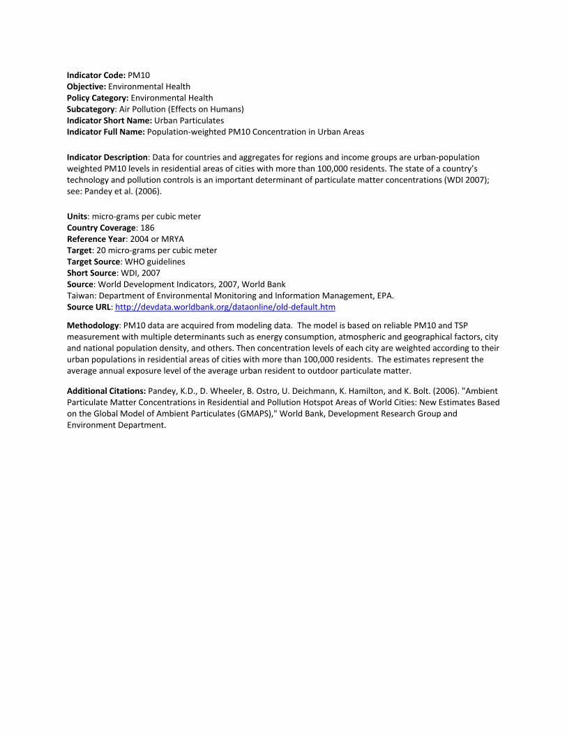
Indicator Code: PM10 Objective: Environmental Health Policy Category: Environmental Health Subcategory: Air Pollution (Effects on Humans) Indicator Short Name: Urban Particulates Indicator Full Name: Population‐weighted PM10 Concentration in Urban Areas
Indicator Description: Data for countries and aggregates for regions and income groups are urban‐population weighted PM10 levels in residential areas of cities with more than 100,000 residents. The state of a country’s technology and pollution controls is an important determinant of particulate matter concentrations (WDI 2007); see: Pandey et al. (2006).
Units: micro‐grams per cubic meter Country Coverage: 186 Reference Year: 2004 or MRYA Target: 20 micro‐grams per cubic meter Target Source: WHO guidelines Short Source: WDI, 2007 Source: World Development Indicators, 2007, World Bank Taiwan: Department of Environmental Monitoring and Information Management, EPA. Source URL: http://devdata.worldbank.org/dataonline/old‐default.htm
Methodology: PM10 data are acquired from modeling data. The model is based on reliable PM10 and TSP measurement with multiple determinants such as energy consumption, atmospheric and geographical factors, city and national population density, and others. Then concentration levels of each city are weighted according to their urban populations in residential areas of cities with more than 100,000 residents. The estimates represent the average annual exposure level of the average urban resident to outdoor particulate matter.
Additional Citations: Pandey, K.D., D. Wheeler, B. Ostro, U. Deichmann, K. Hamilton, and K. Bolt. (2006). "Ambient Particulate Matter Concentrations in Residential and Pollution Hotspot Areas of World Cities: New Estimates Based on the Global Model of Ambient Particulates (GMAPS)," World Bank, Development Research Group and Environment Department.

Indicator Code: INDOOR Objective: Environmental Health Policy CategoryEnvironmental Health SubcategoryAir Pollution (Effects on Humans) Indicator Short Name: Indoor Air Pollution Indicator Full Name: Percentage of Population Using Solid Fuels
Indicator Description: Solid fuels include biomass fuels, such as wood, charcoal, crops or other agricultural waste, dung, shrubs and straw, and coal. The use of solid fuels in households is associated with increased mortality from pneumonia and other acute lower respiratory diseases among children as well as increased mortality from chronic obstructive pulmonary disease and lung cancer (where coal is used) among adults (WHO, 2007).
Units: Percentage of population using solid fuels Country Coverage: 175 Reference Year: 2003 Target: 0 percent Target Source: Expert judgment Short Source: Smith et al., 2004 Source: Smith KR, Mehta S, Maeusezahl‐Feuz M. 2004. Indoor air pollution from household use of solid fuels. In: Comparative Quantification of Health Risks: Global and Regional Burden of Disease Attributable to Selected Major Risk Factors (Ezzati M, Lopez AD, Rodgers A, Murray CJL, eds). Geneva: World Health Organization, 1435‐1493 Taiwan: Department of Environmental Monitoring and Information Management, EPA. Source URL: http://www.who.int/quantifying_ehimpacts/national/countryprofile/mapiap/en/index.html
Methodology: These data were collected from national wide household surveys. The survey data of percentage of solid fuel use population cover 52 countries. The rest of the data are generated from models predicting solid fuel use. The model used SFU values from the household fuel use database, and assumed that as countries develop economically, people gradually shift up an energy ladder from solid fuels to cleaner fuels. The final exposed population is calculated as: Household equivalent solid fuel exposed population = population using solid fuel × ventilation factor.
Additional Citations: Desai, M.A., S. Mehta, K.R. Smith. (2004) Indoor smoke from solid fuels: Assessing the environmental burden of disease. Environmental burden of disease series No. 4. Geneva, World Health Organization. Mehta S, et al. Modeling household solid fuel use towards reporting of the Millennium Development Goal indicator. In press. Energy for Sustainable Development, June 2006. WHO (World Health Organization). 2007, Country Profiles of Environmental Burden of Disease, Available online at http://www.who.int/quantifying_ehimpacts/countryprofiles/en/index.html.

Indicator Code:OZONE_H Objective: Environmental Health Policy Category: Environmental Health Subcategory: Air Pollution (Effects on Humans) Indicator Short Name: Local Ozone Indicator Full Name: Local Ozone with Effects on Human Health
Indicator Description: Population‐weighted accumulated hourly concentrations of high level ozone with a threshold of 85ppb
Units: Exceedance person ppb per capita Country Coverage: 223 Reference Year: 2000 Target: 0 exceedance above 85 pbb Target Source: Expert Judgment Short Source: MOZART‐2 Global Chemical Tracer Model, 2000 Source: Ozone concentrations data: MOZART‐2 Global Chemical Tracer Model, The National Center for Atmospheric Research (NCAR), http://gctm.acd.ucar.edu/mozart/models/m2/index.shtml Source URL: http://gctm.acd.ucar.edu/mozart/models/m2/index.shtml
Methodology: Ozone has an impact on human health and has been associated in epidemiological studies with premature mortality. The health ozone measure was calculated using MOZART‐2 data using the following method: 1) For each grid cell, for each hour in the year, the exceedance (if any) above 85 ppb was calculated. 2) The exceedance value was resampled to 30 arc seconds and overlaid with the GRUMP population data. Exceedance valus were multiplied by population total for each 30‐arc‐second grid cell. 3) Using zonal statistics the excedance‐person‐hous were summed by country. 4)The summed exceedance‐person‐hours were divided by total county population.
Additional Citations Horowitz, L., et al., A global simulation of tropospheric ozone and related tracers: Description and evaluation of MOZART, version 2, J. Geophys. Res., 108(D24), 4784, doi:10.1029/2002JD002853, 24 December 2003.

Indicator Code: OZONE_E Objective: Ecosystem Vitality Policy Category: Ecosystem Impacts of Atmospheric Subcategory: Air Pollution (Effects on Environment) Indicator Short Name: Regional Ozone Indicator Full Name: Regional Ozone with Effects on Ecosystem
Indicator Description: An accumulated exposure concentration over a threshold of 40ppb in daylight time of growing season
Units: Exceedance square‐kilometer‐hours per square kilometer Country Coverage: 223 Reference Year: 2000 Target: 0 exceedance above 3000 ppb.h Target Source: Expert Judgment Short SourceMOZART‐2 Global Chemical Tracer Model, 2000 SourceOzone concentrations data: MOZART‐2 Global Chemical Tracer Model, The National Center for Atmospheric Research (NCAR), http://gctm.acd.ucar.edu/mozart/models/m2/index.shtml Source URL: http://gctm.acd.ucar.edu/mozart/models/m2/index.shtml
Methodology: The ecological ozone measure was calculated using MOZART‐2 data using the following method: 1) We assigned latitudes>0 to the northern hemisphere and latitudes<=0 to the southern. 2) We assigned daylight hours to each band of latitude using information on sunrise and sunset times at: http://aa.usno.navy.mil/data/docs/RS_OneYear.php. 3) We subset the database to include only summer daylight hours (June‐August in the north and December‐February in the south). 4) We summed exceedances above 40 ppb. 5) We multiplied exceedance sums by land area, for each grid cell. 6) Using zonal statistics, we summed these exceedance‐square kilometer products by country. 7) We divided these sums by total country area.
Additional Citations: Horowitz, L., et al., A global simulation of tropospheric ozone and related tracers: Description and evaluation of MOZART, version 2, J. Geophys. Res., 108(D24), 4784, doi:10.1029/2002JD002853, 24 December 2003. International Cooperative Programme on Effects of Air Pollution on Natural Vegetation and Crops. 2007. AOT40 – The Parameter Used to Represent the Accumulated Dose of Ozone. Available at:http://icpvegetation.ceh.ac.uk/8AOT40.htm

Indicator Code: SO2 Objective: Ecosystem Vitality Policy Category: Ecosystem Impacts of Atmospheric Subcategory: Air Pollution (Effects on Environment) Indicator Short Name: Sulfur Dioxide (SO2) emissions Indicator Full Name: Sulfur Dioxide (SO2) emissions per populated land area
Indicator Description: Data used in EDGAR are taken from the best possible international information sources; however it is stressed that the uncertainties in the resulting datasets may be substantial at the country level, especially for methane and nitrous oxide. These uncertainties are due to the limited accuracy of international activity data and, in particular, the emission factors utilized in calculating emissions at the national level. Data presented, however, do provide a reliable dataset for comparability since EDGAR employs methods that are comparable to IPCC methodologies and has global totals that agree with budgets used in other atmospheric studies. In addition to the data reliability issues described above, please see the "Uncertainties" and "Disclaimer" sections of the EDGAR website for more information regarding the various nuances of this dataset. The EDGAR 3.2 database provides global annual emissions per country and on a 1x1 degree grid for 1990 and 1995 for direct greenhouse gases CO2, CH4, N2O and HFCs, PFCs and SF6 and the precursor gases CO, Nox, NMVOC and SO2.” Units: Metric Tons Country Coverage: 215 Reference Year: 2000 Target: 0 Metric Tons Target Source: Expert Judgment Short Source: EDGAR V2.0 by Netherlands National Institute for Public Health and the Environment (RIVM) and the Netherlands Organization for Applied Scientific Research (TNO). Source: EDGAR V2.0 by Netherlands National Institute for Public Health and the Environment (RIVM) and the Netherlands Organization for Applied Scientific Research (TNO). The Netherlands National Institute for Public Health and the Environment/The Netherlands Environmental Assessment Agency (RIVM/MNP) and the Netherlands Organization for Applied Scientific Research (TNO). (2005). The Emission Database for Global Atmospheric Research (EDGAR) 3.2 Fast Track 2000 and 3.2. Acidifying gases: SO2 (Sulfur Dioxide): Extended Emissions 2000 and Aggregated Emissions 1990/1995. The Netherlands, MNP. Source URL: http://www.mnp.nl/edgar/
Methodology: The sulfur dioxide emissions were divided by the land area populated at more than five persons per square kilometer. Total land area was not used in order not to favor countries with very large land areas.
Additional Citations: Olivier, J.G.J., Bouwman, A.F., Berdowski, J.J.M., Veldt, C., Bloos, J.P.J., Visschedijk, A.J.H., Van der Maas, C.W.M. and P.Y.J. Zandveld. (1999). Sectoral emission inventories of greenhouse gases for 1990 on a per country basis as well as on 1o x 1o. Environmental Science & Policy, 2, 241‐264.

Indicator Code: WATQI Objective: Ecosystem Vitality Policy Category: Water SubcategoryWater (Effects on Environment) Indicator Short NameWater Quality Index Indicator Full NameWater Quality Index
Indicator Description: The water quality parameters chosen to be included in the EPI were selected for two reasons. Firstly, they are good indicators of specific issues relevant on a global basis (eutrophication, nutrient pollution, acidification, salinization). Secondly, the parameters were chosen because they are the most consistently reported; that is, we have the most data for these parameters compared to other relevant parameters that were not included. Because water quality is a function of a number of different physical and chemical parameters measured during routine water quality monitoring, as outlined above, a global index of the general status of water quality, ranked on a country by country basis, is best developed as a composite index of several key parameters.
UnitsProximity‐to‐Target Country Coverage: 232: 94 countries with water Reference Year: 2003 (average year for all stations and parameters) Target: proximity‐to‐target score of 100 (based on monitoring station parameter scores) Target Source: Expert judgment and national Short Source: GEMS, 2008 Source: United Nations Environment Program GEMS/Water Programme 2008, online database available at: http://www.gemstat.org European Environment Agency Waterbase Rivers & Lakes data sets, v7 (2007), available at: http://www.eea.europa.eu/themes/water/datasets Taiwan Environmental Protection Administration Executive Yuan, R.O.C. 2005. River and lake water quality data available at: http://edb.epa.gov.tw/eng/Index_water.htm National contacts: Niger: Mr. Ilia Bounari, Hydrochimie à la Division de la Qualité et Pollution des Eaux, Niger Algeria : Mr. Mohamed Ramdane, Agence Nationale des Ressources Hydrauliques, ALGERIE Israel: Dr. Ami Nishri, Kinneret Limnological Laboratory, Israel Oceanographic & Limnological Research Source URL: http://www.gemswater.org/
Methodology: WATQI is a proximity‐to‐target composite indicator with station density adjustment that was calculated as follows. Raw data for five parameters ‐‐ Dissolved Oxygen (DO), Electrical Conductivity (EC), pH, Total Phosphorus (P) (or Ortho Phosphorus), Total Nitrogen (N) (or Dissolved inorganic Nitrogen, Nitrate+Nitrite, or Ammonia) ‐‐ were obtained from UNEP/GEMS Water and European Environmental Agency (EEA) Waterbase, and national sources listed in the source field. The raw data for all parameters except pH and DO were winsorized (trimmed) at the extreme 95th percentile. Then proximity‐to‐target (PTT) values were calculated using the targets specified by UNEP/GEMS water such that 100 corresponds to meeting the target (or falling into the target range in the case of pH) and values between 0 and less than 100 indicate an increasing distance from the target (or target range in the case of pH).
The individual targets used were as follows: DO of 6 mg/L for "warm waters" (>20C) and 9.5 mg/L for "cold waters" (<20C); pH of 6.5‐9.0; EC of 500 micro‐Siemens/cm; P of 0.05 mg/L (or 0.025 for orthohosophate); N of 1 mg/L (or 0.5 for dissolved inorganic N or nitrate+nitrite and 0.05 for ammonia). Total N and Total P are the preferred indicators of nutrient pollution; thus, maximum possible scores for countries that reported other forms of nutrients were adjusted such that the best possible PTT scores for Ortho P and Dissolved inorganic N were set to 80, and for Nitrate+Nitrite and Ammonia were set to 60. Station‐level PTT values were summed and divided by 5 to generate a station‐level WQI that ranged from 0 to 100. Station‐level WQI's were averaged to country WATQI's using only those stations that report the maximum number of parameters within the country.

Country WATQIs were adjusted for density of monitoring stations based on national water quality monitoring data collated by UNEP/GEMS Water. Country WATQI scores were adjusted using the following multipliers based on the density of the monitoring station network per populated land area (land area populated at >5 persons per sq. km, as calculated by CIESIN, 2007). Countries received full credit (using a multiplier of 1) if they have a station density greater than or equal to 1 per 1,000 sq. km; PTT scores were multiplied times 0.95 if they had a station density of 0.1‐0.99 per 1,000 sq. km; PTT scores were multiplied times 0.9 if they had a station density of 0.01‐0.099 per 1,000 sq. km; PTT scores were multiplied times 0.85 if they had a station density of 0.001‐0.0099 per 1,000 sq. km; and PTT scores were multiplied times 0.8 if they had a station density of <0.001 per 1,000 sq. km. We were able to use the above methodology to complete data for 94 countries. For countries with no WATQI from UNEP/GEMS or the EEA, a regional imputed value was used according to this rule: For UNEP‐GEO sub regions with UNEP/GEMS WATQI available for at least half of the countries in that region, the 0.33 percentile WATQI was used; for UNEP‐GEO sub regions with UNEP/GEMS WQI available for less than half of the countries in that region but more than 3 WQIs, the average minus a 10 point penalty was used. For remaining regions, we applied the following method: for Meso‐America the average of available WQI's for Meso and North America minus a 10pt penalty was used; for Eastern Africa, we took the average for Kenya and Uganda and applied a 10 point penalty; for Southern Africa we took the average for South Africa and Tanzania and applied a 10 point penalty; for Central Africa we took the score for the Democratic Republic of Congo and applied a 10 point penalty; for Centeral Asia we took the average of the 33rd percentile score for South Asia and the score for Russia with a 10 point penalty; for the Caribbean we took the score for Cuba with 10 point penalty; for the South Pacific we took the average scores for Fiji and Papua New Guinea and applied a 10 point penalty; for the Arabian Peninsula & Mashriq, we took the average scores for Iraq and Jordan and applied a 10 point penalty. Additional Citations: Center for International Earth Science Information Network (CIESIN), Columbia University, (2007). National Aggregates of Geospatial Data: Population, Landscape and Climate Estimates, v. 2 (PLACE II), Palisades, NY: CIESIN, Columbia University. Available at: http://sedac.ciesin.columbia.edu/place/.

Indicator Code: WATSTR Objective: Ecosystem Vitality Policy Category: Water Subcategory: Water (Effects on Environment) Indicator Short Name: Water Stress Indicator Full Name: Percentage of National Territory Experiencing Water Stress (withdrawals exceed 40% of available supply)
Indicator Description: The EPI water stress indicator is the percentage of a country’s territory affected by oversubscription of water resources. A high degree of oversubscription is indicated when the water use is more than 40% of available supply (WMO, 1997). Countries can to some extent accommodate oversubscription in one region with inter‐basin transfers, water re‐use and desalination but some of these engender significant environmental impacts of their own. Thus, the ultimate target for each country is to have no area of their territory affected by oversubscription.
Units: Percentage of national territory with water withdrawals exceeds 40% of available supply Country Coverage: 171 Reference Year: Contemporary (mean annual 1950‐1995) Target: 0 percent Target Source: Expert Judgment Short Source: University of New Hampshire, Water Systems Analysis Group. Source: University of New Hampshire, Water Systems Analysis Group. Source URL: http://www.watsys.sr.unh.edu
Methodology: Human water demand was computed using the following data sources: population per grid cell; per capita country or sub national level domestic water demand; per capita country or sub national level industrial water demand; irrigated land extent per grid cell according to Döll et al. (2000); and country or sub national level agricultural water demand (irrigation). Global discharge fields were computed by blending mean annual discharge observations (where available) with a climatology (1950‐1995) of discharge output from the Water Balance Model based on Vörösmarty et al. (1998). An indicator of relative water demand (RWD) for each 1/4 degree grid cell was computed by dividing total human water demand (domestic + industrial + agricultural water or DIA) by renewable water supply (Q). RWD = 0.4 was established as the threshold for water stressed conditions. The percentage of territory in which water resources are oversubscribed was computed by summing the area of grid cells in each country where RWD >= 0.4. Details on the computation and use of RWD (alternatively known as the Relative Water Stress Index or RWSI) can be found in Vörösmarty et al. (2000) and Vörösmarty et al. (2005). Additional Citations Döll, P., Siebert, S. 2000. A digital global map of irrigated areas. ICID Journal, 49(2), 55‐66. Vörösmarty, C. J., C. A. Federer and A. L. Schloss. (1998). Evaporation functions compared on US watershed: Possible implications for global‐scale water balance and terrestrial ecosystem modeling, Journal of Hydrology, 207 (3‐4): 147‐169. WMO (World Meteorological Organization).et al. (1997). Comprehensive Assessment of the Freshwater Resources of the World. Geneva, Switzerland. Vörösmarty, C. J., P. Green, J. Salisbury and R. B. Lammers. (2000). Global water resources: vulnerability from climate change and population growth, Science, 289:284‐288. Vörösmarty, C. J., E. M. Douglas, P. Green and C. Revenga. (2005). Geospatial Indicators of Emerging Water Stress: An Application to Africa, Ambio, 34 (3): 230‐236.

Indicator Code: CRI Objective: Ecosystem Vitality Policy Category: Biodiversity and Habitat SubcategoryBiodiversity and Habitat Indicator Short NameConservation Risk Index Indicator Full Name: Ratio of Protected to Converted Lands Indicator Description: The Conservation Risk Index measures the ratio of protected to converted lands and is calculated by WWF biome within each country. It compares the area of each biome in the country that is under protection to the area of each biome that has been converted to other land uses (e.g., from forests to cropland). This indicator is a more comprehensive measure of whether countries are protecting their natural environment on the same spatial scale as habitats are being converted.
Units: Ratio Country Coverage: 205 Reference Year: 2006 for protected areas, 2000 for land cover Target: 0.5 Target Source: Expert Judgment Short Source: The Conservation Strategies Division of The Nature Conservancy calculated this indicator based on third party source data. Source: Calculations by Timothy Boucher of the Conservation Strategies Division, The Nature Conservancy, based on these data sets: UNEP‐WCMC (United Nations Environment Programme‐World Conservation Monitoring Center). (2007). Global Protected Areas Data Set extracted from the World Database on Protected Areas (WDPA) in August 2007 by UNEP World Conservation Monitoring Centre (WDPA custodian) (www.unep‐wcmc.org), Cambridge, UK. Joint Research Centre. Global Land Cover 2000. Available at http://www‐gvm.jrc.it/glc2000/. (Note: the USA, Central America and Australia portions of the GLC200 were updated by TNC using more recent and finer resolution data. The sources include the National Land‐cover Dataset of the U.S. (Vogelmann 2001), regional datasets for Mesoamerica (Mas et al., 2002; World Bank 2001), National Vegetation Information System (NVIS) Australasia, 2000.) World Wildlife Fund. (2001). Terrestrial Ecoregions of the World. Available from http://www.worldwildlife.org/science/ecoregions.cfm Source URL: www.unep‐wcmc.org; http://www.worldwildlife.org/science/ecoregions.cfm
Methodology: The CRI value per country‐biome is based on two 1 km global spatial datasets: the World Database on Protected Areas (2007), which reports the location and distribution of protected areas, and an updated version of the Global Land Cover 2000 data set, which provides the areas of natural habitat converted to human uses versus those not converted to human uses. The target for the Conservation risk index is the global average ratio of 1:2 (protected lands : converted lands). A ratio of protected to converted of less than 0.5 reflects poor performance in protecting a particular terrestrial biome. A score above 0.5 reflects a better than average performance in protecting a given biome. For example, the CRI for the Namibian Tropical Grasslands is 1.4 (i.e. 9.3% Protected and 6.6% Converted), which is a good performance rating. The method for calculating CRI (Hoekstra et al. 2005) was implemented as the ratio between the percent of protected area per country‐biome and the percent of converted land per country‐biome. Data were generated at a 1 km level of resolution and percent values derived at the country‐biome unit of analysis. The World Database on Protected Areas (2007), which gives us the protected vs. non‐protected areas was processed as follows: (1) only National PAs were used (no international PAs); (2) PAs were removed that had the following Status: "proposed", "voluntary" or "recommended"; (3) only PA points that did not have polygons and did not have a status according
to #2 were buffered according to their defined area (using a Mollweide Projection); (4) the buffered points and polygons datasets were merged for the final WDPA dataset; and (5) an Arcinfo GRID with a 1km resolution was created from the final protected areas mask, with a value of 0 for unprotected and 1 for protected. For the reclassified and updated GLC2000, an Arcinfo GRID was created with a value of 0 for unconverted lands, and a value of 1 for converted lands. The zonal mean was calculated for each GRID for the WWF‐biome‐country dataset (the union of the country dataset and the WWF biome dataset). Calculating the zonal mean of each GRID by country‐biome (pixel value 0 or 1) results in a value that can be used a percentage. Note: For the country‐biome units that were smaller than what can be reasonable calculated from the 1 km spatial data, areas were counted as ‘no data’. Given their size the resulting indicator should not be impacted. Additional Citations: Hoekstra et al. 2005 National Vegetation Information System (NVIS) ‐ Australasia, 2000. http://www.deh.gov.au/erin/nvis/index.html Vogelmann, J.E., S.M. Howard, L. Yang, C.R. Larson, B.K. Wylie, N. Van Driel. (2001). Completion of the 1990s National Land Cover Data Set for the Conterminous United States from Landsat Thematic Mapper Data and Ancillary Data Sources, Photogrammetric Engineering and Remote Sensing, 67, pp. 650‐652. Mas, J.‐M., Velazquez, A., Palacio‐Prieto, J.L., Bocco, G., Peralta, A., and Prado, J. (2002). Assessing forest resources in Mexico: wall‐to‐wall land use/cover mapping. Photogrammetric Engineering & Remote Sensing, Vol. 68, No. 10, pp. 966‐1000.

Indicator Code: EFFCON Objective: Ecosystem Vitality Policy Category: Biodiversity and Habitat Subcategory: Biodiversity and Habitat Indicator Short Name: Effective Conservation Indicator Full Name: Effective Conservation by Biome
Indicator Description: This indicator measures the percentage habitat by biome that has been effectively conserved within each biome by country. The effective conservation index gives a protected area value for each terrestrial biome within a country by spatially overlaying three 1 km global spatial datasets, the World Database on Protected Areas (2007), the Wildlife Conservation Society/CESIN Human Footprint (2007), and biomes from the WWF Ecoregions of the World dataset (Olson et al., 2001). By combining these measures the index provides a measure of how much habitat within protected areas is actually intact or relatively intact (i.e., has a low human footprint). The World Database on Protected Areas (2007) is a dataset on the location and distribution of protected areas. The CIESIN/Wildlife Conservation Society Human Footprint is a dataset on human impacts on land, measured by transportation networks (roads, railroads and rivers), population densities, and urban areas. The Human footprint is used here to classify locations that are either under high or low threat/use by humans. Areas within a designated protected area that have a high human footprint(one which is incompatible with biodiversity) are deducted from the protected area, with the effect of lowering the area of specific biomes identified as protected within that country. This is a better measure of the amount of land under protection because it accounts for areas that are not fully protected because of land conversion, roads, and populated places that might exist within a protected area. All three datasets are widely accepted and used, even though as all other global databases they do have limitations relative to the resolution of the data and problems with protected area delineations. The effective conservation target is 10% of each terrestrial biome within a country. In order to ensure that above target performance for one biome does not mask below target performance for another, performance is capped at 10% for each biome. This target is based upon the internationally agreed upon target set by the Convention on Biological Diversity. Units: Percentage Territory Country Coverage: 233 Reference Year: 2007 Target: 10 percent Target Source: Convention on Biological Short Source: The Conservation Strategies Division of The Nature Conservancy calculated this indicator based on third party source data. Source: Calculations by Timothy Boucher of the Conservation Strategies Division, The Nature Conservancy, based on three data sets: UNEP‐WCMC (United Nations Environment Programme‐World Conservation Monitoring Center). (2007). Global Protected Areas Data Set extracted from the World Database on Protected Areas (WDPA) in August 2007 by UNEP World Conservation Monitoring Centre (WDPA custodian) (www.unep‐wcmc.org), Cambridge, UK. CIESIN and Wildlife Conservation Society. (2007). Human Footprint v.2 (beta). Available from http://sedac.ciesin.columbia.edu/wild_areas/. World Wildlife Fund. (2001). Terrestrial Ecoregions of the World. Avaialble from http://www.worldwildlife.org/science/ecoregions.cfm Source URL: www.unep‐wcmc.org; http://sedac.ciesin.columbia.edu/wild_areas/.; http://www.worldwildlife.org/science/ecoregions.cfm

Methodology: The Effective Conservation value per country‐biome is based on three 1 km global spatial datasets: World Database on Protected Areas (2007), which gives us the protected vs. non‐protected areas; (b) the CIESIN and Wildlife Conservation Society Human Footprint (2007) which, by using statistic natural breaks and calibrated with known areas, was reclassified into high or low threat/use by humans; and (c) biomes from the WWF Ecoregions of the World dataset (Olson et al., 2001). The following specific steps were taken. The World Database on Protected Areas (2007) was processed as follows: (1) only National PAs were used (no international PAs); (2) PAs were removed that had the following Status: "proposed", "voluntary" or "recommended"; (3) only PA points that did not have polygons and did not have a status according to #2 were buffered according to their defined area (using a Mollweide Projection); (4) the buffered points and polygons datasets were merged for the final WDPA dataset; and (5) an Arcinfo GRID with a 1km resolution was created from the final protected areas mask, with a value of 0 for unprotected and 1 for protected. By using statistic natural breaks and calibrated with known areas, the CIESIN and Wildlife Conservation Society Human Footprint(2007) was reclassified into high or low threat/use by humans. TNC classified the continuous index data of the Human Influence Index according to frequency distribution and variance using Jenk’s Natural Breaks. The 0‐24 range of values was identified as a surrogate for the least threatened and human‐impacted areas. This class not only encompasses the "Last of the Wild" (Sanderson et al. 2002) areas, but also includes areas with low levels of human population that are distant from human access points, such as roads. Index values equal or above the 25 mark were identified as moderately to heavily impacted. This class includes all human‐disturbed areas ‐ those within and nearby roads, populated places, and agriculture. The reclassified HII was reclassified using the following values: a 1 for low and a 0 for high. Multiplying the two datasets (using the Spatial Analysis Tool in Arcinfo) produced a final GRID with areas that are (a) protected and have a low threat/use have a value of 1, and (b) other areas (those with high threat/use or unprotected) resulted in a value of 0. The zonal mean was calculated using the final GRID for the Country‐Biome dataset. Calculating the Zonal Mean of the GRID by Country‐Biome (pixel value 0 or 1) results in a value that can be used a percentage. The effective conservation target is 10% of land by biome conserved within a country. Protection by biome is capped at 10% so that countries cannot offset less than 10% protection of any given biome with greater than 10% protection in another. Caveats: All three datasets are widely accepted and used, even though as with all other global databases they do have limitations relative to the resolution of the data and problems with protected area delineations. Further spatial errors can arise in the overlay process, especially for the smallest island nations. Additional Citations Olson, D.M., E. Dinerstein, E.D. Wikramanayake, et al. (2001). Terrestrial Ecoregions of the World: A New Map of Life on Earth, Bioscience 51(11), pp. 933‐938. Sanderson, E.W., M. Jaiteh, M.A. Levy, K.H. Redford, A.V. Wannebo, and G. Wolmer. (2002). "The Human Footprint and the Last of the Wild," BioScience, Vol. 52, No. 10, pp. 891‐904.

Indicator Code: AZE Objective: Ecosystem Vitality Policy Category: Biodiversity and Habitat Subcategory: Biodiversity and Habitat Indicator Short Name: Critical Habitat Protection Indicator Full Name: Percent of Alliance for Zero Extinction Sites Protected
Indicator Description: Percent of Alliance for Zero Extinction (AZE) Sites Protected is designed to give more rigorous insight into the protection of highly endangered species. It catalogs whether countries provide protection for sites designated by the Alliance for Zero Extinction (AZE). Indices that look at species conservation by country can be difficult to develop, as the percentage of endangered species within a country is tied to the natural endowment of the country. Moreover, species are assessed as threatened on the basis of their global conservation status. This means that even if a country takes extensive measures to protect that species in its own territory, they might still rank poorly on an index that looks at the percentage of endangered species at the global level. The Alliance for Zero Extinction is a joint initiative of 52 biodiversity conservation organizations, which aims to prevent extinctions by identifying and safeguarding key sites, each one of which is the last remaining refuge of one or more Endangered or Critically Endangered species. They follow the IUCN Red List criteria for Endangered or Critically Endangered species; therefore it uses a consistent and standardized approach and criteria across the world. To date, AZE has identified 595 sites that each represents the last refuge of one or more of the world’s most highly threatened species.
An AZE site must meet all three of the following criteria:
a) Endangerment. An AZE site must contain at least one Endangered (EN) or Critically Endangered (CR) species, as listed by IUCN ‐ World Conservation Union.
b) Irreplaceability. An AZE site should only be designated if it is the sole area where an EN or CR species occurs, or contains the overwhelmingly significant known resident population of the EN or CR species, or contains the overwhelmingly significant known population for one life history segment (e.g., breeding or wintering) of the EN or CR species.
c) Discreteness. The area must have a definable boundary within which the character of habitats, biological communities, and/or management issues have more in common with each other than they do with those in adjacent areas. Units: Percentage Country Coverage: 86 Reference Year: 2004 Target: 100% Target Source: Expert Judgment Short Source: Conservation Strategies Division, The Nature Conservancy. Source: Results based on Ricketts et al., 2005. Source URL: not available
Methodology: We calculated the percent of AZE sites within each country that are within a protected area, based on the published paper by Ricketts et al. (2005).
Additional Citations: Ricketts, T.H., et al. (2005). Pinpointing and preventing imminent extinctions. Proceedings of the National Academy of Sciences, 51, pp. 18497‐18501.
Indicator Code: MPAEEZ Objective: Ecosystem Vitality Policy Category: Biodiversity and Habitat Subcategory: Biodiversity and Habitat Indicator Short Name: Marine Protected Areas Indicator Full Name: Percentage of Exclusive Economic Zone (EEZ) Area that is Protected
Indicator Description: Home to mangroves, sea grasses, coral reefs, and other critical habitats, coastal areas are vital to marine biodiversity. There is growing recognition of the need to protect coastal and marine resources from over‐fishing and other activities the damage habitat. This indicator represents a simple assessment of the percent area in each country's exclusive economic zone that is protected. The target is set to 10%, the same as for terrestrial protected areas.
Units: Percentage area Country Coverage: 132 Reference Year: 2006 Target: 10% Target Source: Convention on Biological Short Source: Suzanne Mondoux and Louisa Wood, Fisheries Centre, University of British Columbia Source: Data compiled by Suzanne Mondoux and Louisa Wood, Fisheries Centre, University of British Columbia. Original data developed in a collaboration between the Sea Around Us Project, World Wildlife Fund (WWF), United Nations Environment Programme ‐ World Conservation Monitoring Centre (UNEP‐WCMC) and the World Conservation Union ‐ World Commission on Protected Areas (IUCN‐WCPA). Source URL: http://www.mpaglobal.org/
Methodology: Protected areas were coded as marine if they principally cover the marine portion of the coastal zone. The area of marine protected areas was tallied and divided by the total area in a country's exclusive economic zone (EEZ). For countries with more than one EEZ, the MPA area and EEZ areas were summed, and then the total area protected was divided by the combined total EEZ area for the country.
Additional Citations Wood, L. J. (2007). MPA Global: A database of the world's marine protected areas. Sea Around Us Project, UNEP‐WCMC & WWF. Available at http://www.mpaglobal.org

Indicator Code: FORGRO Objective: Ecosystem Vitality Policy Category: Productive Natural Resources Subcategory: Forestry Indicator Short Name: Change in Growing Stock Indicator Full Name: Change in the Volume of Growing Stock
Indicator Description: Growing stock is defined as the standing tree volume of the forest resources. An increase in growing stock usually means higher quality forests, whereas a decrease in growing stock generally indicates degrading forest conditions. For simplicity in measurement and explanation of the forest resources condition, growing stock is a good choice. Caveats: Although growing stock is important, standing tree volume alone is not sufficient for a detailed analysis. For example, future wood supply is highly dependent on the age class distribution, or the stand structures and the management system applied. Further, biodiversity requires diversity, e.g., in tree species and succession stages. Carbon storage is highly dependent on soil carbon, which may not be directly correlated to tree volume. Finally, converting primary forests to forest plantations may increase the tree volume but it generally degrades the condition (related to biodiversity and ecosystems) of the natural habitat. Units: cubic meters/hectare Country Coverage: 127 (deforestation data were used to increase country coverage to 230) Reference Year: 2005:2000 Target: No Decline Target Source: Expert Judgment Short Source: Forestry Department, Food and Agricultural Organization of the United Nations Source: Food and Agricultural Organization of the United Nations. (2005). Global Forests Resources Assessment 2005. Rome, FAO. Source URL: http://www.fao.org/forestry/site
Methodology: Growing stock is a volumetric measure that measures the cubic meters of wood over bark of all living trees more than X cm in diameter at breast height. It includes the stem from ground level or stump height up to a top diameter of Y cm, and may also include branches to a minimum diameter of W cm. Countries indicate the three thresholds (X, Y, W in cm) and the parts of the tree that are not included in the volume. Countries must also indicate whether the reported figures refer to volume above ground or above stump. The diameter is measured at 30 cm above the end of the buttresses if these are higher than 1 meter. Growing stock includes windfallen living trees but excludes smaller branches, twigs, foliage, flowers, seeds, and roots. The ratio of growing stock in cubic meters was taken for 2005 and 2000. Ratios greater than 1 indicate that the growing stock increased over the time period, and ratios less than 1 indicate that it decreased. Countries with a growing stock of 1 or greater were taken to be "at target". Countries with declining growing stock were considered to be below target. For Germany, the ratio of 2000 to 1990 data was used instead. For countries without growing stock data, data on percent change in forest area were used. The correlation between growing stock and deforestation data is very high (excluding three outliers, Comoros, Indonesia, and Micronesia, the R2 = 0.81, p<.001, ), so this was determined to be a robust way to impute the value fo change in growing stock. Additional Citations: not available

Indicator Code: MTI Objective: Ecosystem Vitality Policy Category: Productive Natural Resources Subcategory: Fisheries Indicator Short NameMarine Trophic Index Indicator Full Name: Slope of Marine Trophic Index from 1950‐2004 Indicator Description: The marine trophic level ranges from 1 in plants to 4 or 5 in larger predators. It expresses the relative position of fish and other animals in the hierarchical food chain that nourish them. They provide food for small fish which, have a trophic level of about 3,and the small fish are eaten by slightly larger fish that have a trophic level of 4, which, in turn, are what large predators such as sharks and marine mammal and humans typically eat (Pauly and MacLean 2003). If the average level at which a country’s fisheries is catching fish declines over time, it means that the overall the trophic structure of the marine ecosystem is becoming depleted of larger fish higher up the food chain, and is resorting to smaller fish. This indicator measures the slope of the trend line in the Marine Trophic Index (MTI) from 1950‐2004. If the slope is 0 or is positive, the fishery is either stable or improving. If the slope is negative (below 0), it means the fishery is declining, and that smaller and smaller fish are being caught. Units: Slope of Trend Line Country Coverage: 134 Reference Year: 1950‐2004 Target: No Decline Target Source: Expert Judgment Short Source: Sea Around Us Project and the Convention on Biological Diversity Source: Sea Around Us Project and the Convention on Biological Diversity Source URL: http://www.seaaroundus.org/
Methodology: Using the Sea Around Us website, data were gathered on the slope of the trend line in the Marine Trophic Index (MTI) from 1950to 2004 for a country's exclusive economic zones (EEZs). For countries with more than one EEZ, a weighted average slope was calculated on the basis of the relative size of the EEZs. Data for Albania were only available through 1970 and data for Eritrea were only available through 1978.
Additional Citations Pauly, D., and J.L. MacLean. (2003). In a Perfect Ocean: The State of Fisheries and Ecosystems in the North. Washington, DC, Island Press. Pauly, D. and Watson, R. (2005). Background and interpretation of the 'Marine Trophic Index' as a measure of biodiversity. Philosophical Transactions of The Royal Society: Biological Sciences 360: 415‐423.

Indicator Code: EEZTD Objective: Ecosystem Vitality Policy Category: Productive Natural Resources Subcategory: Fisheries Indicator Short Name: Trawling Intensity Indicator Full Name: Percentage of Exclusive Economic Zone Area Trawled
Indicator Description: Benthic trawling is a fishing method that targets fish and invertebrates that inhabit ocean floor (or benthic) ecosystems. These include cod, scallops, shrimp, and flounder. Such trawling comes at a heavy environmental cost. Bottom trawling and dredging equipment has been described as the most destructive fishing gear in use today (Watson, 2004 and 2006). Benthic trawls are boats equipped with large heavy nets that are dragged across the living seafloor. The nets are held open at the front by a metal beam or by large "doors", which can weigh several tons, and which are designed to scour the bottom as the trawl is dragged along, forcing the fish and invertebrates up into the net. This process exerts a heavy toll on the natural habitats of the sea floor, breaking off brittle bottom flora and fauna such as sponges and corals. Marine species such as turtles that try to escape the gear suffer stress, injury, and quite frequently, death (FAO, 2005). The damage can last many years and continuous trawling and dredging does not allow the time needed for habitat recovery. Deep‐sea coral communities can be wiped out by a single trawl sweep and repeated trawling can change the species composition of the ecosystem toward small opportunistic species, such as sea stars and small short‐lived clams, and diminishes the abundance of commercially valuable species. In addition to disrupting the living seafloor, trawling kills a large number of animals as "by catch," the accidental harvest of untargeted species, such as other fish and invertebrate species, marine mammals, seabirds, and turtles. Some of this by catch is retained for sale, but a portion of it is returned to the sea, usually dead or dying. These animals returned to sea are known as discards. Bottom trawled fisheries have the highest discard rates of all fisheries. By catch is a contributor to the depletion of fish stocks, and can have a significant impact on endangered species of fish, mammals, turtles and seabirds. The habitat destruction caused by trawling and dredging directly affects the human communities that depend on marine resources for food and income. Key nursery habitats such as seagrass are essential for sustaining a range of commercially important species. When these nursery habitats are destroyed, the entire local environment is impacted and the productivity of local fisheries, including those employing sustainable fishing methods, decreases. The 2008 EPI uses a simple calculation of the percentage of the shelf area in each country’s EEZ that is fished by trawlers. There are no direct data available for the area trawled on a country‐by‐country basis. However, there are good data available describing fish landings and the gear used to catch these fish, and acceptable data on the composition of each country’s fishing fleet. Units: Percentage Area Country Coverage: 175 Reference Year: 2004 Target: 0% Target Source: Expert Judgment Short Source: Watson et al. 2004; 2006 Source: Watson, R., Hoshino, E., Beblow, J., Revenga, C., Kura, Y., & Kitchingman, A. (2004). Fishing gear associated with global marine catches. Fisheries Centre Research Reports 12(6), 32p. Watson, R., Revenga, C., & Kura, Y. (2006). Fishing gear associated with global marine catches: II Trends in trawling and dredging. Fisheries Research 79, 103‐111. Source URL: http://www.seaaroundus.org/

Methodology: This indicator is calculated based on the amount of catch that is trawled per one‐half degree (30 arc‐minute) grid cells. This results in a metric of the area (sq km) associated with combined bottom trawl or dredge catch (supergears 8 or 9) rates >0.05 tonnes/sq km/year within declared EEZ areas. The marine area of the cells are added up to find the total area trawled and then divided by total EEZ. Cells that have a minimal catch are not included in the analysis.
Additional Citations: FAO. (2005). Mortality of fish escaping trawl gears (No. 478). Rome:Food and Agriculture Organization of the United Nations.
Indicator Code: IRRSTR Objective: Ecosystem Vitality Policy Category: Productive Natural Resources Subcategory Agriculture Indicator Short Name: Irrigation Stress Indicator Full NamePercentage of Irrigated Area that is in Water Stressed Areas
Indicator Description: Agriculture is by far the largest user of "blue water" (freshwater in streams, lakes, from groundwater aquifers, etc) globally, with irrigation accounting for 70% of freshwater extraction globally and as much as 80‐90% in some developing countries. When water is abstracted for irrigation in water stressed areas (catchments in which consumption exceeds 40% of available water supplies) , it can contribute to seasonal low‐flows, and to excessive concentration of agrochemicals from agricultural runoff. This indicator simply measures the percentage of irrigated agriculture that falls in areas of water stress within a country. Units: Percentage Area Country Coverage: 159 Reference Year: circa 2000 Target: 0% Target Source: Expert Judgment Short Source: CIESIN calculation based on global irrigation map by Johann Wolfgang Goethe University and Food and Agriculture Organization of the UN, and water stressed area map by University of New Hampshire Water Systems Analysis Group. Source: CIESIN calculation based on three data sets: Johann Wolfgang Goethe University and Food and Agriculture Organization of the UN, Global Map of Irrigation Areas version 4.0.1, available at: http://www.fao.org/nr/water/aquastat/irrigationmap/index10.stm University of New Hampshire Water Systems Analysis Group, Mean annual relative water stress index (unitless ratio per grid cell),available at http://wwdrii.sr.unh.edu/ Country Grid (CIESIN 2006): Country grid with cell size of 0.083333. Grid values are UNSD codes
Source URL: http://www.fao.org/nr/water/aquastat/irrigationmap/index10.stm; http://wwdrii.sr.unh.edu/
Methodology: The Global Map of Irrigation Areas version 4.0.1, with a spatial resolution of 5 arc‐minutes, was overlaid on the global map of mean annual relative water stress index, with a spatial resolution of 30 arc‐minutes. The irrigated area that fell in water stressed grid cells was summed and divided by the total irrigated area for the country in order to calculate the percentage of irrigated area that is in water stressed areas. The specific processing steps were as follows: 1. Resampled the UNH Relative Water Stress data at 0.083333 grid cell size to match that of the Global Map of Irrigated Areas 2. Reclassify the Relative Water Stress data into the following classes a. 1: grid value < 40% b. 2:grid value >= 40% 3. Calculate Irrigation area within each class 4.Summary area irrigated in each country using Zonal Statistics
Additional Citations: Siebert, S., P. Döll, S. Feick, J. Hoogeveen and K. Frenken. (2007). Global Map of Irrigation Areas version 4.0.1. Johann Wolfgang Goethe University, Frankfurt am Main, Germany / Food and Agriculture Organization of the United Nations, Rome, Italy.

Indicator Code: AGSUB Objective: Ecosystem Vitality Policy Category: Productive Natural Resources Subcategory: Agriculture Indicator Short Name: Agricultural Subsidies Indicator Full Name: Agricultural Subsidies represented by Nominal Rates of Assistance(NRA) by country
Indicator Description: According to a report by the OECD (2004), agricultural subsidies exacerbate environmental pressures through the intensification of chemical use and the expansion of land into sensitive areas. This indicator seeks to assess the magnitude of subsidies in order to assess the degree of environmental pressure they exert. The NRA is defined as the price of their product in the domestic market (plus any direct output subsidy) less its price at the border, expressed as a percentage of the border price (adjusting for transport costs and quality differences).
Units: Proximity‐to‐Target, with 100 being the target, and 0 being the worst performer Country Coverage: 238 Reference Year: 2005 Target: 100 Target Source: Expert Judgment Short Source: YCELP calculation based on OECD Producer Support Estimates Data, WDR 2008 and the Pilot 2006 EPI Source: World Development Report Selected Indicators 2008, OECD Producer Support Estimates database 2007, Pilot 2006 EPI Source URL: http://siteresources.worldbank.
Methodology: Where available, we used data on the Nominal Rate of Assistance (NRA) from the World Development Report 2008. NRA is defined as the price of a product in the domestic market, less its price at a country’s border, expressed as a percentage of the border price, and adjusted for transport costs and quality differences (WDR 2008). These were converted to the standard EPI proximity‐to‐target indicator. NRA data were unavailable for a number of countries for which we had data when we compiled the Pilot 2006 EPI (Costa Rica, Israel, Jordan, Peru, Tunisia, Uruguay, and Venezuela). For these , the indicator was computed by subtracting greenbox subsidies from total agricultural subsidies, which was then divided by the total value of agriculture. Low and middle‐income countries without agricultural subsidies data were imputed a proximtity to target score of 0 on the basis that most non‐OECD countries do not subsidize their agricultural sector. Caveats: Combining the 2008 EPI data with the AGSUB indicator data from the 2006 EPI represented a less than perfect solution, yet we were uncomfortable assigning a score of 100 to countries that subsidize their agriculture, and unwilling to estimate subsidy levels for countries that are engaged in agriculture of dubious environmental sustainability. This methodology makes use of the best data available, and we hope to include a more accurate measure in future editions of the EPI, as improved data sources arise. Additional Citations Agriculture’s "multifunctionality" and the WTO; Kym Anderson; The Australian Journal of Agricultural and Resource Economics, 44:3, pp 475‐494
Indicator Code: AGINT Objective: Ecosystem Vitality Policy Category:Productive Natural Resources Subcategory: Agriculture Indicator Short Name: Intensive Cropland Indicator Full Name: Percentage of Cropland Area that is in Agriculture‐dominated Landscapes
Indicator Description: As a rough rule of thumb, ecologists agree that if more than 30% of the area of a given landscape is under intensive use for agricultural production, then major ecosystem functions will likely be compromised, and if this level reaches 60%, then special attention is needed to conserve ecosystem functions (Wood et al., 2000). The 2008 EPI sets a target of 40% uncultivated land in areas of crop production, although this figure includes grazing land and settlements, so is quite conservative. The indicator considers whether each 10km x 10km grid cell where cropping occurs has at least 40% land uncultivated, thereby "making space" for other ecosystem functions. If agriculture makes up more than 60% of the grid cell, the agricultural land in that grid cell is considered to be intensive. The indicator seeks to address the problem of over‐clearing, excessive "in‐filling" of agricultural landscapes. Units: Percentage Area Country Coverage: 158 Reference Year: 2000 Target: 0% Target Source: Expert Judgment Short Source: CIESIN calculation based on global cropland grid by Ramankutty et al. (forthcoming). Source: CIESIN calculation based on global cropland grid from Ramankutty et al. (forthcoming). Source URL: not available
Methodology: Global cropland grids by Ramankutty et al. (forthcoming) representing the proportion of land that is in cropland per 5 arc‐minute grid cell were processed to calculate two figures, the total cropland area per country, and the total cropland area per country in grid cells in which cropland represents more than 60% of land use types in that grid cell. The latter was divided by the former and multiplied by 100 to calculate the percentage of cropland area that is in agriculture dominated landscapes. Countries with less than 3,000 sq. km of cropland were considered not to have sufficient cropland for this indicator, and were considered therefore to have no data. Additional Citations Ramankutty, N., A.T. Evan, C. Monfreda, J.A. Foley. (forthcoming). Farming the Planet. Part 1: The Geographical Distribution of Global Agricultural Lands in the Year 2000. Global Biogeochemical Cycles, in press. Wood, S., K. Sebastian, and S. Scherr. 2000. Pilot Analysis of Global Ecosystems: Agroecosystems. IFPRI and WRI, Washington, DC.
Indicator Code: PEST Objective: Ecosystem Vitality Policy Category: Productive Natural Resources Subcategory: Agriculture Indicator Short Name: Pesticide Regulation Indicator Full Name: Degree of Regulation of Toxic Pesticides
Indicator Description: Pesticides are a significant source of pollution in the environment, affecting both human and ecosystem health. Pesticides damage ecosystem health by killing beneficial insects, pollinators, and fauna they support. Human exposure to pesticides has been linked to increases in headaches, fatigue, insomnia, dizziness, hand tremors, and other neurological symptoms. Furthermore, many of the pesticides included in this index are persistent organic pollutants (POPs), endocrine disruptors, or carcinogens. Our indicator of pesticide use examines the legislative status of countries on two landmark agreements on pesticide usage, the Rotterdam and Stockholm conventions, and also rates the degree to which these countries have followed through on the objectives of the conventions by limiting or outlawing the use of certain toxic chemicals. While the Rotterdam convention focuses on trade restrictions and proper labeling of toxic substances, the Stockholm convention seeks to limit or ban the use of the 12 most toxic persistent organic pollutants which bio accumulate and move long distances in the environment. While ideally, we would use an output measure rather than a legislative measure for this indicator, we concluded after extensive research that the robust data on pesticide usage ‐ especially for banned pesticides for which official data may be scant ‐ were simply not available. While legislative controls do not always match the situation on the ground, this indictor sends a clear message to countries that setting standards for pesticides use is an essential first step in controlling the degree to which toxics are used at a national scale. Units: 22 Point Scale, with 0 representing the lowest score, and 22 the highest Country Coverage: 238 Reference Year: 2003 Target: 22 points Target Source: Expert Judgment Short Source: YCELP calculation based on data from the Rotterdam Convention and the Stockholm Convention. Source: YCELP calculation based on data from the Rotterdam Convention and the Stockholm Convention. Source URL: Rotterdam Convention. Available at http://www.pic.int/home.php?type=t&id=5&sid=16. Stockholm Convention on Persistent Organic Pollutants (POPs). Available at http://www.pops.int/.
Methodology: The indicator encompasses 11 criteria, each of which have a maximum of two possible points. The first two criteria measure whether, and to what degree countries have participated in the conventions. Under the Rotterdam Convention, countries receive 2 points if they are a party and have designated a national authority for its implementation, 1 point if they are a party but have no national authority, and 0 points if they are not a party. Under the Stockholm Convention on Persistent Organic Pollutants, countries receive 2 points if they are a party and have created a national implementation plan (NIP), 1 point if they are a party but have no NIP, and 0 points if they are not a party. These data are available via the respective convention secretariats. The next nine criteria indicate whether countries have banned (for a score of 2), restricted (for a score of 1), or taken no action (for a score of 0) on regulating the nine of the "dirty dozen" persistent organic pollutants. These include aldrin, chlordane, DDT, dieldrin, endrin, heptachlor, hexachlorobenzene, mirex, and toxaphene. Data for these criteria were collected from the United Nations Environment Programme Chemicals. Country performance is a simple sum of the scores across the 11 criteria for a maximum possible score of 22. Additional Citations United Nations Enviroment Programme, Chemicals. Master List of Actions on the Reduction and/or Releases of Persistent Organic Pollutants. June 2003

Indicator Code: BURNED Objective: Ecosystem Vitality Policy Category:Productive Natural Resources Subcategory: Agriculture Indicator Short Name: Burned Area Indicator Full Name: Percentage of Country Area Burned
Indicator Description: Biomass burning has long been recognized as a significant source of carbon emissions that contribute to climate change, and as an important source of airborne particulates, especially in developing countries. Thus, from atmospheric perspective, it is unambiguously negative. From a land management perspective, however, the role of biomass burning in soil fertility management and ecosystem processes is more difficult to assess. For example, controlled biomass burning in the agricultural sector, on a limited scale, can have positive functions as a means of clearing and rotating individual plots for crop production, and in some ecosystems, as a healthy means of weed control and soil fertility improvement. In a number of natural ecosystems, such as savannah and scrub forests, wild fires can help maintain biotic functions. However, in tropical forest ecosystems, fires are mostly human induced and environmentally harmful, killing wildlife, reducing habitat, and setting the stage for more fires by reducing moisture content and increasing combustible materials. Even where fire can be beneficial from an agricultural perspective, fires can inadvertently spread to natural ecosystems, setting the stage for further agricultural colonization. Hence, we have chosen to asess fires as, on balance, a negative phenomenon from an agricultural natural resource management perspective.
Units: Percentage Country Coverage: 160 Reference Year: 2005‐2006 Target: 0 Target Source: Expert Judgment Short Source: L3JRC 2000‐2007, CIESIN, 2007 Source: Joint Research Centre’s Global Burnt Areas 2000‐2007 (L3JRC) CIESIN Global Rural‐Urban Mapping Project (GRUMP) land area and country grids. Source URL: not available
Methodology: The EPI team assessed the extent of burn scars by downloading and processing data for 2000 (representing April 2000‐March 2001) and 2005 (representing April 2005‐March 2006) from the Joint Research Centre’s Global Burnt Areas 2000‐2007 (L3JRC)product, which identifies burnt areas using the SPOT VEGETATION sensor at 1km resolution. These data were simplified to a boolean surface of burnt (1) and non‐burnt (0) areas and subsampled from 0.009 degree resolution to 0.008 degrees to match the Global Rural‐Urban Mapping Project (GRUMP) land area and country grids. The total burnt area was calculated by multiplying the boolean burnt area grid by the GRUMP land area grid (land area in ha) and summing the results. The country totals were generated by calculating the unique combination of countries (from GRUMP) and burnt areas, then summing the land area grid for the country‐burnt area zones. We calculated total land area burnt for the 12 months from April 2000‐March 2001 and April 2005‐May 2006 in order to assess land burning during two years under different climate regimes: for the winter of 2000‐01 there was a strong La Niña signal in the Pacific Ocean, and for the winter of 2005‐06 neither El Niño or La Niña played a role in global climate patterns. We calculated the land area burned as a percentage of total land area in both years, then averaged the percentages. Additional Citations Tansey, K., Grégoire, J.M.C., Defourny, P., Leigh, R., Pekel, van Bogaert, E., Bartholomé, E., Bontemps, S. 2008. A new, global,multi‐annual (2000‐2007) burned area product at 1 km resolution and daily intervals. Geophysical Research Letters, Vol. 35, L01401, doi:10.1029/2007GL031567

Indicator Code: GHGCAP Objective: Ecosystem Vitality Policy Category: Climate Change Subcategory: Climate Change Indicator Short Name: Emissions Per Capita Indicator Full Name Greenhouse Gas Emissions Per Capita Indicator Description: Sum of emissions of six greenhouse gases, in CO2 equivalents, and emissions attributable to land use, divided by total population. Units: Metric Tons C02 Equivalent Per Person Country Coverage: 169 Reference Year: 2005:2000 Target: 2.24 Metric Tons C02 Equivalent Target Source: Calculated by calculating 50% Short Source: IAE, 2007, Houghton 2003, IMF 2005 Source: International Energy Agency. CO2 Emissions from Fuel Combustion (2004 edition). International Monetary Fund, World Economic Outlook Database, October 2007 Population year 2005 Houghton, R.A. 2003. Revised estimates of the annual net flux of carbon to the atmosphere from changes in land use and land management 1850‐2000. Tellus 55B:378‐ 390. Source URL: http://wds.iea.org/WDS/TableViewer/dimView.aspx?ReportId=949
Methodology: For countries missing GHG emission data, values were imputed using a regression model predicting GHG emissions fom CDIAC CO2 emissions. For countries missing land‐use emissions, values were imputed based on the regional average of land‐use emissions were square kilometer. GHG emissions and land‐use emissions were summed and divided by 2005 population.
Additional Citations: not available
Indicator Code: CO2KWH Objective: Ecosystem Vitality Policy Category: Climate Change Subcategory: Climate Change Indicator Short Name: CO2 from Electricity Production Indicator Full Name: Emissions per Kilowatt Hour of Energy Produced
Indicator DescriptionSum of emissions from combustion of all fossil fuel types used for public electricity generation, public combined heat and power generation, and public heat plants.
Units: g CO2 per kWh Country Coverage: 213 Reference Year: 2005 Target: 0 Target Source: Expert Judgment Short Source: IAE, 2007 Source: International Energy Agency. CO2 Emissions from Fuel Combustion (2004 edition). Source URL: http://wds.iea.org/WDS/TableViewer/dimView.aspx?ReportId=949
Methodology: This data includes emissions from public elec. and heat producers. Carbon dioxide emissions from public electricity and heat production include the sum of emissions from combustion of all fossil fuel types used for public electricity generation, public combined heat and power generation, and public heat plants. Public utilities are defined as those undertakings whose primary activity is to supply the public. Emissions from electricity and heat production for use by the producer (autoproduction) are not included in this variable, as those emissions are attributed to industry, transport or "other" sectors. CO2 from public electricity and heat production corresponds to International Panel on Climate Change (IPCC) Source/Sink Category 1 A 1 a
Additional Citations: not available

Indicator Code: CO2IND Objective: Ecosystem Vitality Policy Category: Climate Change Subcategory: Climate Change Indicator Short Name: Industrial Carbon Intensity Indicator Full Name: Carbon Emissions from Industry per Industrial GDP
Indicator Description: Total emissions from industry sector, divided by industrial GDP.
Units: CO2 per $1000, USD 1995 PPP Country Coverage: 170 Reference Year: 2005 Target: .85 Target Source: 27% of current, reduction that Short Source: IAE, WDI, 2007 Source: International Energy Agency. CO2 Emissions from Fuel Combustion (2004 edition). World Development Indicators, Percentage of GDP from Industry, 2005
Source URL: http://wds.iea.org/WDS/Report
Methodology: For countries with missing data, values were imputed based on regression model predicting CO2IND using CO2_GDP (CO2 emissions per GDP). Industrial GDP were calculated based on the percentage of GDP from industry, and total GDP. IAE industrial CO2 emissions were divided by industrial GDP to create the indicator.
Additional Citations: not available