environmental conscious highway design for vertical crest curves _al... · 2011-11-21 · 28...
TRANSCRIPT

Environmental Conscious Highway Design for Vertical Crest Curves
by
Mr. Myunghoon Ko* Zachry Department of Civil Engineering
Texas A&M University, TAMU 3136 College Station, TX 77843-3136
Phone: (979) 845-9882 E-mail: [email protected]
Dr. Dominique Lord Zachry Department of Civil Engineering
Texas A&M University, TAMU 3136 College Station, TX 77843-3136
Phone: (979) 458-3949 Fax: (979) 845-6481
E-mail: [email protected]
Dr. Josias Zietsman Environment and Air Quality Division
Texas Transportation Institute The Texas A&M University System
3135 TAMU College Station, TX 77843-3135
Phone: (979) 458-3476 Fax: (979) 845-7548
E-mail: [email protected]
November 7, 2011
Word Count: 5,499 + 4 Tables + 4 Figures = 7,499
*Corresponding author
ABSTRACT 1 2
The primary objective of this paper was to provide guidelines and tools for quantifying the 3 environmental impacts, by means of fuel consumption and emissions, of various highway 4 geometric design conditions related to vertical crest curves. Second-by-second speed profiles 5 were generated with the speed prediction and polynomial models, and fuel consumption and 6 emissions rates based on vehicle-specific power and speeds were extracted using the recently 7 developed motor vehicle emission simulator (MOVES). The generated speed profiles were 8 matched with the extracted rates and aggregated during a trip on the curves. A benefit-cost 9 analysis was also carried out using existing data from the State of Washington. The results 10 demonstrated that the design vehicle respectively consumed and produced 10 percent less fuel 11 and carbon dioxide on the vertical crest curve designed with 1.5 times greater than the minimum 12 rate of vertical curvature value documented in the Green Book; for other emissions – carbon 13 monoxide, oxides of nitrogen, hydrocarbons, and particulate matter of 2.5 microns or less – there 14 were also reductions by up to 31 percent on the curve. The results also showed that the 15 environmental economic benefits from flattening the curve design exceeded addition 16 construction costs for a 30-year design period. In conclusion, vertical curve design providing a 17 flatten curvature can be environmentally and economically beneficial throughout the life of the 18 highway. Finally, this paper shows the efficacy of environmentally-friendly design for 19 sustainable transportation. 20
Ko, Lord, & Zietsman 1
INTRODUCTION 1 Surface transportation is a major contributor to energy consumption and air pollution and 2 accounts for about one-third of greenhouse gas (GHG) emissions emitted in the U.S., according 3 to the U.S. House of Representatives Committee on Science and Technology (1). Multiple 4 strategies (e.g., public transportation, smart growth, alternative transportation mode, high-5 occupancy toll (HOT)/high-occupancy vehicle (HOV) lanes) should be considered to address 6 these challenges. Increasing capacity by constructing new highways, widening existing 7 highways, or improving highway design features are also key strategies. Considering the 8 significant impact, environmentally sustainable highways will be a main objective in developing 9 new highways or improving existing ones. 10
During the highway design process, the reference most often used by designers and 11 engineers for design features and criteria is the Green Book, also known as A Policy on 12 Geometric Design of Highways and Streets, published by the American Association of State 13 Highway and Transportation Officials (2). It is a series of guidelines on geometric design, 14 providing a range or a minimum for desirable design standards (3). When the applied design 15 criteria do not meet the standards, a design exception is usually required. The range or minimum 16 guidelines and design exception provide designers and engineers with flexibility regarding 17 geometric situations in the highway design process. For instance, the Texas Department of 18 Transportation (TxDOT) Roadway Design Manual (4) recommends that use of higher rather than 19 the minimum design standards results in a safer environment, better compensating for drivers’ 20 errors. 21
In addition to providing a recommended range or minimum values for critical dimensions, 22 if design guidebooks/manuals were to provide any quantitative analysis of each design 23 criteria/features on safety, it could reduce the uncertainty associated with making engineering 24 judgment for given design criteria/features. For example, some guidebooks/manuals (e.g., 25 Highway Safety Manual (5)) have recently provided quantitative analysis between design criteria 26 and specific features, such as safety. The TxDOT Roadway Design Manual (4) specified a 27 vertical alignment design in which the length of the ascending grade should consider a heavy 28 truck operation without an undesirable speed reduction, typically 15 km/h, below the average 29 running speed of traffic. This manual does not provide any quantitative information on the 30 impacts of roadway grades on safety. However, Bonneson et al. (6) intended to provide 31 quantitative safety design guidelines and evaluation tools to be used by designers and engineers. 32 They reported that 16 percent more crashes occurred on an eight-percent grade relative to a flat 33 or leveled section of freeway. If a vertical alignment design has a flatter grade than the allowable 34 maximum standard, it could significantly increase the construction costs, but at the same time, it 35 will reduce the crash risk and societal costs throughout the life of the highway. There is a similar 36 issue in the environmental analysis. As long as highway design manuals/guidebooks do not 37 provide any information regarding the quantitative environmental impacts of highway geometric 38 design features on fuel consumption and emissions, the matter of environmental issues related to 39 the selected design features is completely dependent upon engineering judgment. 40
The objectives of this study were to: 1) analyze the impacts of vertical crest curve design 41 features on fuel consumption and emissions using the recently developed vehicle emissions 42 model and speed profiles generated by the speed prediction and polynomial models; 2) show that 43 the degree of fuel consumption and emissions could be changed by varying specific highway 44 geometric design values with the conceptual evaluation tool such as modification factors; 3) 45 propose practical methods and processes of speed profiles and emissions rates for 46
Ko, Lord, & Zietsman 2
designers/engineers to apply for other geometric design conditions/features; and 4) evaluate the 1 environmental impacts of actual vertical curve data using the proposed methods and processes. 2
This paper focuses only on the quantitatively environmental analyses on vertical crest 3 curves under the selected design and traffic conditions; the environmental evaluation of other 4 conditions (e.g., various truck proportions), other features (e.g., horizontal curves), and the 5 detailed procedures for quantifying environmental impacts as part of the highway design process 6 can be found in the original dissertation (7). The results provided in this study are beneficial for 7 highway designers and engineers by providing the guidelines and evaluation tools on the 8 environmental impacts related to the selection of highway geometric design conditions/features; 9 therefore, it can reduce the uncertainty in engineering judgment for environmentally-conscious 10 highway design. Second, this study shows the importance of the environmental effect of highway 11 design, and supports the statement that environmentally-friendly highway design can be one 12 strategy for sustainable transportation. The next section describes the background on the factors 13 affecting fuel consumption and emissions. 14 15 BACKGROUND 16 The U.S. Environmental Protection Agency’s motor vehicle emissions simulator (MOVES) 17 model is based on vehicle-specific power (VSP), because VSP quantifies vehicle emissions and 18 fuel consumption related to various vehicle characteristics and operating conditions (8, 9). VSP 19 (kW/ton) is defined as the instantaneous power per unit mass of vehicle as shown in Eq. (1). 20
21
(1) 22
23 where, 24
V = vehicle speed (m/s); 25 a = vehicle acceleration (m/s2); 26 Ar = rolling resistance coefficient (kW/m/s); 27 B = speed correction to rolling resistance coefficient (kW/(m/s)2); 28 C = air drag resistance coefficient (kW/(m/s)3); 29 M = vehicle mass (ton); 30 g = gravitational constant (9.81 m/s2); and, 31 Θ = roadway grade (degree). 32
33 Vehicle speed was a key variable in measuring a vehicle’s operating conditions and 34
predicting fuel consumption and emissions (10). Barth and Boriboonsomsin (10) concluded that 35 carbon dioxide (CO2) emission rates were highly dependent on speed; traveling at a steady-state 36 speed (around 72-to-80 km/h) resulted in lower emissions and fuel consumption compared with 37 speeds exceeding 105 km/h or below 72 km/h. Vehicle speed was expressed as a second-by-38 second variable, because average speed was not adequate for evaluation of the impacts of 39 highway geometric design and traffic-signal control on emissions and fuel consumption. This 40 was due to the lack of accounting for vehicle driving dynamics, such as acceleration or 41 deceleration (8, 11, and 12). Servin et al. (11) analyzed how much fuel consumption and 42 emissions could be reduced by intelligent speed adaptation (ISA) that regulates speed variation 43 in driving, and found that the ISA significantly saved fuel and reduced CO2 by approximately 37 44 percent and 35 percent, respectively. Strategies regulating vehicle speeds, such as the ISA, were 45 closely linked with acceleration because regulating speed variation could be achieved by 46
Ko, Lord, & Zietsman 3
reducing the frequencies of acceleration. Ahn et al. (13) and Qi et al. (12) developed the 1 microscopic emissions models that predict vehicle fuel consumption and emissions using 2 instantaneous speed and acceleration/deceleration as explanatory variables. These models more 3 accurately predicted fuel consumption and emissions as compared to the measured data. 4
Several studies concluded that roadway grade was one of the key variables affecting fuel 5 consumption and emissions, as were vehicle speed and acceleration. Boriboonsomsin and Barth 6 (14) and Park and Rakha (15) analyzed the impacts of roadway grades on fuel consumption and 7 emissions. According to Boriboonsomsin and Barth (14), a vehicle consumed 15-to-20 percent 8 more fuel on an uphill route at a six-percent grade followed by downhill route at a six-percent 9 grade than on flat route. The larger amount of fuel consumed going uphill was not fully 10 compensated for by the smaller amount of fuel consumption going downhill. They concluded 11 that speed and acceleration had a large impact on vehicle fuel consumption and tailpipe 12 emissions, and found that roadway grade was one of the primary variables that determine the 13 power requirements necessary for specific driving maneuvers. 14 15 METHODOLOGY 16 This section describes the speed prediction and polynomial models used to collect second-by-17 second speed profiles along vertical crest curves. Emissions rates from MOVES are then 18 matched with the generated speed profiles and calculated emissions per second are aggregated 19 along traveled distance and time. 20 21 Speed Prediction Model 22 Fitzpatrick et al. (16) provided a speed prediction model (Eq. (2)) for predicting operating speeds 23 of passenger vehicles at the middle of vertical crest curves on two-lane rural highways, in which 24 the predicted operating speed was dependent on the rate of vertical curvature (K). 25
26
105.08 . (K ≤ 39) (2) 27
28 For trucks, they did not provide a model because of the limited amount of measured data. 29
According to the Green Book (2), the truck operation of the larger and heavier units than 30 passenger vehicles needed longer braking distances; however, higher height of truck driver’s eye 31 allowed seeing farther beyond vertical sight obstructions. The longer braking distance and higher 32 height in truck operations balanced with the shorter braking distance and lower height in 33 passenger vehicles. In addition, the Green Book did not provide separate design criteria for truck 34 and passenger vehicles on vertical curves. Thus, the authors of this paper assumed that trucks 35 had same speed profiles as passenger vehicles for the benefit-cost analysis. 36
The predicted operating speeds based on the model were classified as spot speeds at the 37 middle of vertical crest curves. However, vehicles did not move at constant speeds on vertical 38 curves. To consider speed variation on the curves, this study expressed vehicle speed as a 39 second-by-second variable along a traveled distance/time, and the instantaneous speeds were 40 calculated from acceleration/deceleration rates based on the polynomial model. 41
42 Polynomial Model 43 In real-life driving, the curve representing the relationship between acceleration and time 44 typically had a bell-shape and S shape for speed and time curve (17, 18); these curve shapes 45 described that acceleration rates were zero at the start and end of acceleration and supported the 46
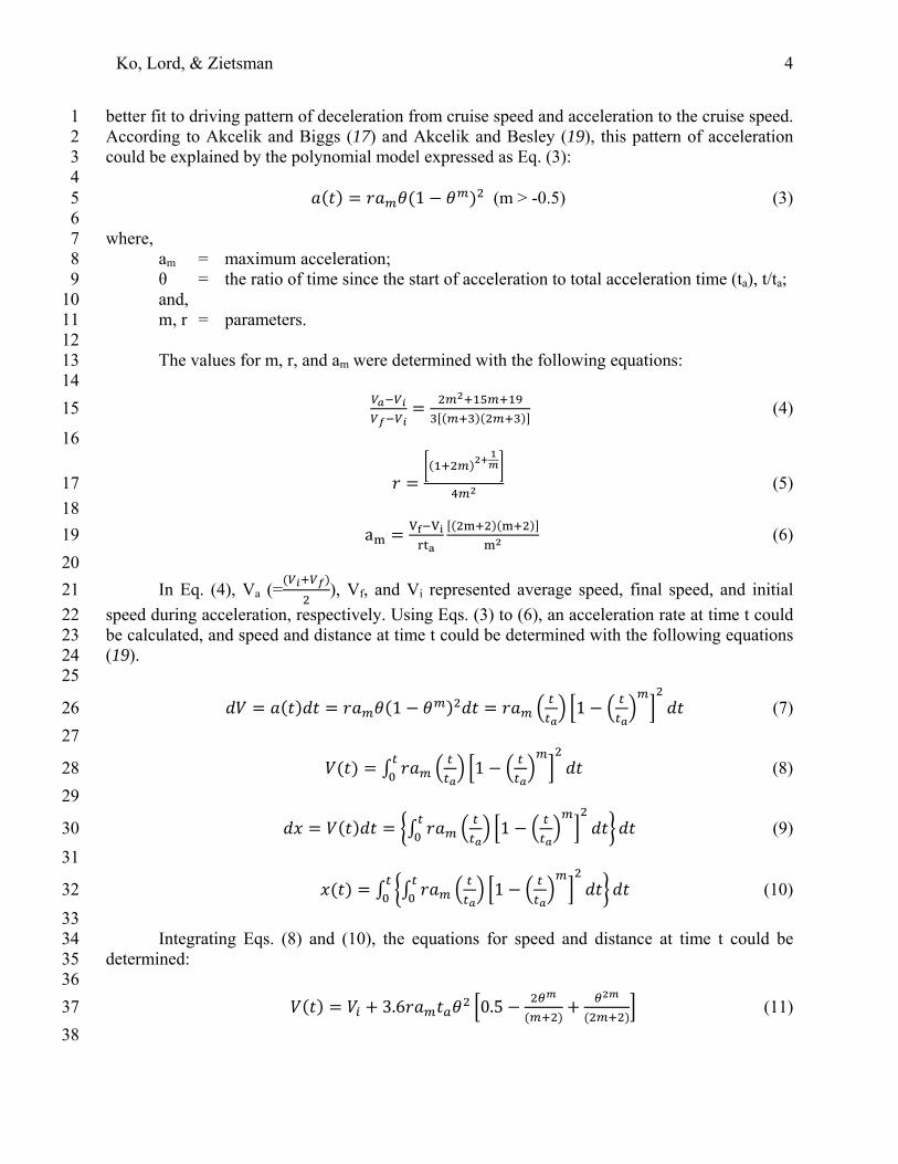
Ko, Lord, & Zietsman 4
better fit to driving pattern of deceleration from cruise speed and acceleration to the cruise speed. 1 According to Akcelik and Biggs (17) and Akcelik and Besley (19), this pattern of acceleration 2 could be explained by the polynomial model expressed as Eq. (3): 3 4
1 (m > -0.5) (3) 5 6 where, 7
am = maximum acceleration; 8 θ = the ratio of time since the start of acceleration to total acceleration time (ta), t/ta; 9 and, 10 m, r = parameters. 11
12 The values for m, r, and am were determined with the following equations: 13
14
(4) 15
16
(5) 17
18
a (6) 19
20
In Eq. (4), Va (= ), Vf, and Vi represented average speed, final speed, and initial 21
speed during acceleration, respectively. Using Eqs. (3) to (6), an acceleration rate at time t could 22 be calculated, and speed and distance at time t could be determined with the following equations 23 (19). 24 25
1 1 (7) 26
27
1 (8) 28
29
1 (9) 30
31
1 (10) 32
33 Integrating Eqs. (8) and (10), the equations for speed and distance at time t could be 34
determined: 35 36
3.6 0.5 (11) 37
38

Ko, Lord, & Zietsman 5
. (12) 1
2 These equations were based on the known acceleration time (ta). When the acceleration 3
time and distance were unknown, the regression equation (Eq. (13)), provided by Akcelik and 4 Biggs (17), for acceleration time could be used. 5 6
. . / . (13) 7
8 9 Motor Vehicle Emission Simulator (MOVES) 10 Based on instantaneous vehicle speeds and VSPs, MOVES categorized operating modes for 11 predicting running exhaust emissions into 23 bins. Since MOVES did not directly report the 12 emissions rates for each bin, this study used a project-level analysis, a single model year, and a 13 single operating mode distribution (i.e., one for the target bin and zero for the remainder). The 14 repetitive processing by changing the target bin generated the fuel consumption and emissions 15 rates for each of the 23 operating mode bins. The extracted fuel consumption and emissions rates 16 were based on two types of vehicles, a passenger car and heavy-duty diesel truck, in Jefferson 17 County, Washington (Table 1). 18
Fuel consumption and emissions were aggregated during travel times based on the 19 second-by-second operating mode bins from the speed profiles and the rates for each operating 20 mode bin. This process could be expressed as following: 21
22 ∑ , (14) 23
24 where, 25
Etype = total emission for each of CO2, oxides of nitrogen (NOx), carbon monoxide 26 (CO), hydrocarbons (HC), particulate matter of 2.5 microns or less (PM2.5), or total fuel 27 consumption; and, 28 etype, bin = fuel consumption or emission rate for operating bin at time t. 29

Ko, Lord, & Zietsman 6
TABLE 1 Basic Condition for MOVES Processing 1 Variable Specification
Input
Vehicle
Type A Single Passenger Car
A Single Heavy Duty Truck
Mass (ton)Passenger Car 1.478 Heavy-Duty
Truck 31.404
Model Year
Passenger Car 4 yrs old Heavy-Duty
Truck 4 yrs old
Fuel Passenger Car
Conventional Gasoline (Market share: 28 percent)
Gasohol (E10) (Market share: 72 percent)
Heavy-Duty Truck
Conventional Diesel Fuel
Roadway Type Rural Unrestricted Access Grade Level
Area Jefferson County, WA Year 2010
month May Temperature (°F) 60.8 Relative Humidity
(percent) 63.9
Output Fuel Consumption
Rate (gal/s) on each operating mode by each vehicle type
Emissions Rates (g/s) of CO2, NOx, HC, CO, and PM2.5 on each operating mode by each vehicle type
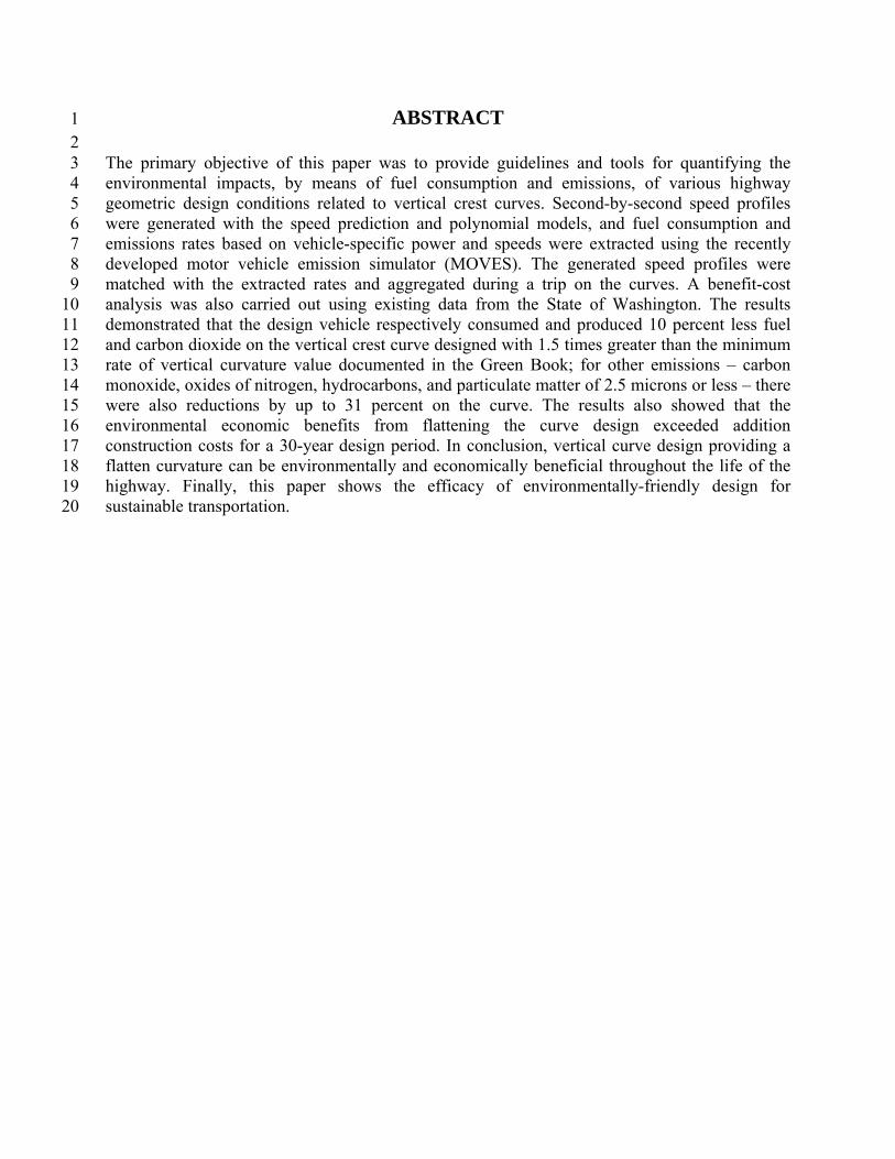
2 DATA SIMULATION 3 The second-by-second speed profiles with various Ks were based on the trip by a passenger car 4 that is the design vehicle on the vertical curve design. The Green Book recommended the 5 minimum K of 39 m/percent for the design speed of 90 km/h (2). Although the vertical crest 6 curve should be designed with a greater K-value than the minimum standard documented in the 7 Green Book, a highway section might be designed with values lower than the minimum 8 standards. Additional explanations on this issue would be presented with actual highway 9 geometric data in the later section. The authors considered the cases of the below- and above-10 design using a K-value lower and greater than the minimum standards in the Green Book (2), 11 respectively. Figure 1 illustrates the base conditions and assumptions for the speed profiles on 12 vertical crest curve in a two-lane highway. 13
Ko, Lord, & Zietsman 7
1
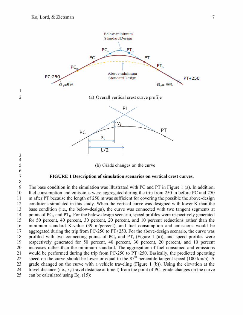
(a) Overall vertical crest curve profile 2
3 4
(b) Grade changes on the curve 5 6
FIGURE 1 Description of simulation scenarios on vertical crest curves. 7 8 The base condition in the simulation was illustrated with PC and PT in Figure 1 (a). In addition, 9 fuel consumption and emissions were aggregated during the trip from 250 m before PC and 250 10 m after PT because the length of 250 m was sufficient for covering the possible the above-design 11 conditions simulated in this study. When the vertical curve was designed with lower K than the 12 base condition (i.e., the below-design), the curve was connected with two tangent segments at 13 points of PCu and PTu. For the below-design scenario, speed profiles were respectively generated 14 for 50 percent, 40 percent, 30 percent, 20 percent, and 10 percent reductions rather than the 15 minimum standard K-value (39 m/percent), and fuel consumption and emissions would be 16 aggregated during the trip from PC-250 to PT+250. For the above-design scenario, the curve was 17 profiled with two connecting points of PCo and PTo (Figure 1 (a)), and speed profiles were 18 respectively generated for 50 percent, 40 percent, 30 percent, 20 percent, and 10 percent 19 increases rather than the minimum standard. The aggregation of fuel consumed and emissions 20 would be performed during the trip from PC-250 to PT+250. Basically, the predicted operating 21 speed on the curve should be lower or equal to the 85th percentile tangent speed (100 km/h). A 22 grade changed on the curve with a vehicle traveling (Figure 1 (b)). Using the elevation at the 23 travel distance (i.e., xt: travel distance at time t) from the point of PC, grade changes on the curve 24 can be calculated using Eq. (15): 25

Ko, Lord, & Zietsman 8
100.
(15) 1
2 where G0 was 9 percent and A was the algebraic difference of the approach and departure 3
tangent grades (G2- G1). Additionally, Et was the elevation at the distance of xt from the point of 4 PC. 5
6 Procedures for Second-by-Second Speed Profiles 7 The speed profiles related with various K-values were developed with the following procedure. 8 9
1. Predict the operating speed at vertical crest curve and calculate the length of vertical 10 curvature (L = KA=K|G2-G1|). For example: 11 12
105.08149.6920
≅ 97 /
13 20 ∗ | 9 9| 351
14
2. Determine the deceleration time (Eq. (13)) with the predicted operating speed (Vf) at 15 the middle of curve and approaching tangent speed (Vi). 16 17
. . / .≅ 6 seconds 18
19 Based on the calculations above, the vehicle would decelerate from 100 km/h (Vi) to 20 97 km/h (Vf) in six seconds. 21
3. Calculate the speeds and travel distance every second using the following equations. 22 For example, acceleration rate, speed, and distance at three second after beginning a 23 deceleration on the curve: 24
25 3 1 0.2185 /
26
3 3.6 0.5 =98.7 km/h 27
28
3.
=81.8 m 29
30
where m = 3.2122, am = -0.2203, and r = 2.4929 would be calculated from Eqs. (4) to 31 (6). 32
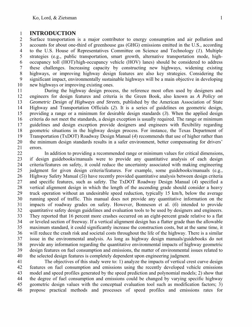
4. Grade per second would be calculated using Eq. (15). Figure 2 (a) describes the 33 changes of grades on the curves. 34
35
36
Ko, Lord, & Zietsman 9
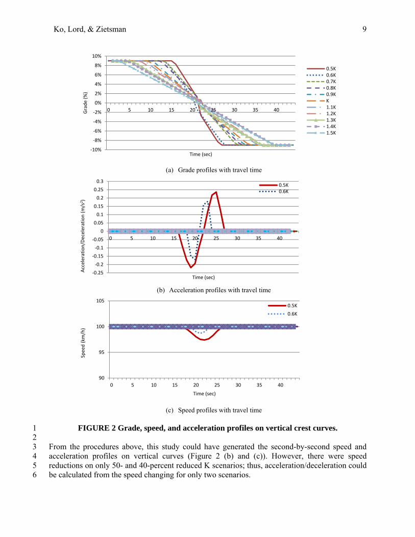
(a) Grade profiles with travel time
(b) Acceleration profiles with travel time
(c) Speed profiles with travel time
FIGURE 2 Grade, speed, and acceleration profiles on vertical crest curves. 1 2 From the procedures above, this study could have generated the second-by-second speed and 3 acceleration profiles on vertical curves (Figure 2 (b) and (c)). However, there were speed 4 reductions on only 50- and 40-percent reduced K scenarios; thus, acceleration/deceleration could 5 be calculated from the speed changing for only two scenarios. 6
‐10%
‐8%
‐6%
‐4%
‐2%
0%
2%
4%
6%
8%
10%
0 5 10 15 20 25 30 35 40Grade (%
)
Time (sec)
0.5K0.6K0.7K0.8K0.9KK1.1K1.2K1.3K1.4K1.5K
‐0.25
‐0.2
‐0.15
‐0.1
‐0.05
0
0.05
0.1
0.15
0.2
0.25
0.3
0 5 10 15 20 25 30 35 40
Acceleration/Deceleration (m/s
2)
Time (sec)
0.5K0.6K
90
95
100
105
0 5 10 15 20 25 30 35 40
Speed (km
/h)
Time (sec)
0.5K
0.6K

Ko, Lord, & Zietsman 10
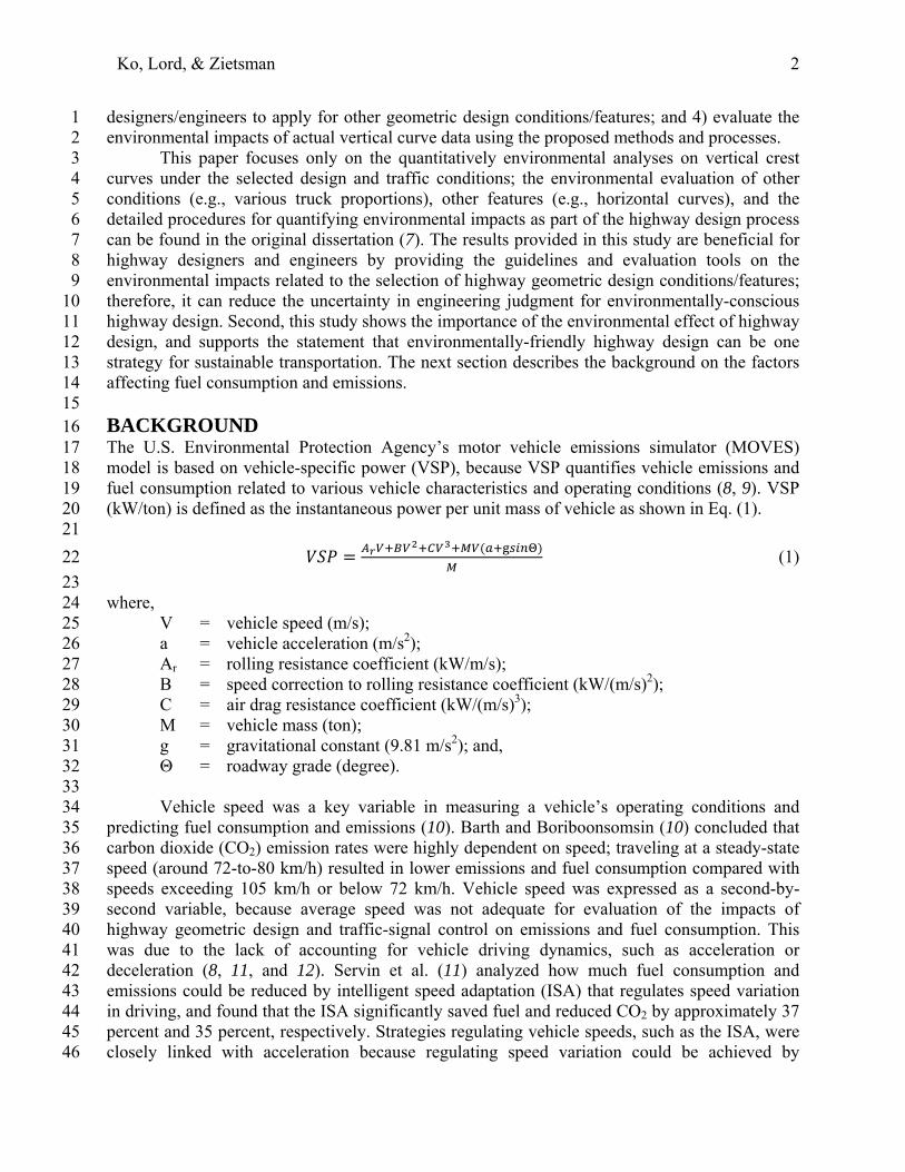
Fuel Consumption and Emissions Rates from MOVES 1 This section provides the rates of fuel consumption and emissions on the 23 operating mode bins 2 from the MOVES processing. Figure 3 shows the fuel consumption and emissions rates for each 3 of the 23 operating mode bins from the passenger car (Car) and heavy-duty diesel truck (HDDT). 4 The fuel consumption and emissions rates increased linearly or exponentially with their VSPs 5 within certain range. Higher engine load that can be represented by higher VSP directly resulted 6 in the higher rates through the combustion process. 7 8
(a) Fuel Consumption (Car) (b) Fuel Consumption (HDDT)
(c) CO2 (Car) (d) CO2 (HDDT)
(e) NOx (Car) (f) NOx (HDDT)
FIGURE 3 Fuel consumption and emissions rates for each operating mode bin.
0
0.0002
0.0004
0.0006
0.0008
0.001
0.0012
0.0014
0.0016
0 111
12
13
14
15
16
21
22
23
24
25
27
28
29
30
33
35
37
38
39
40
Fuel Consumption (gal/s)
VSP Bin
0
0.002
0.004
0.006
0.008
0.01
0.012
0 1 11
12
13
14
15
16
21
22
23
24
25
27
28
29
30
33
35
37
38
39
40
Fuel Consumption (gal/s)
VSP Bin
0
2
4
6
8
10
12
14
16
0 111
12
13
14
15
16
21
22
23
24
25
27
28
29
30
33
35
37
38
39
40
CO2 (g/s)
VSP Bin
0
20
40
60
80
100
120
0 111
12
13
14
15
16
21
22
23
24
25
27
28
29
30
33
35
37
38
39
40
CO2 (g/s)
VSP Bin
0
0.001
0.002
0.003
0.004
0.005
0.006
0.007
0.008
0.009
0.01
0 1 11
12
13
14
15
16
21
22
23
24
25
27
28
29
30
33
35
37
38
39
40
NOx (g/s)
VSP Bin
0
0.05
0.1
0.15
0.2
0.25
0.3
0.35
0.4
0.45
0 1
11
12
13
14
15
16
21
22
23
24
25
27
28
29
30
33
35
37
38
39
40
NOx (g/s)
VSP Bin

Ko, Lord, & Zietsman 11
(g) CO (Car) (h) CO (HDDT)
(i) HC (Car) (j) HC (HDDT)
(k) PM2.5 (Car) (l) PM2.5 (HDDT)
FIGURE 3 Continued. 1 SIMULATION RESULTS 2 This section documents the results on the aggregated fuel consumption and emissions from the 3 combination of the rates (gal/s and g/s) with the second-by-second speed profiles and shows the 4 comparison analysis between the aggregated results by environmental modification factors 5 (EMFs). These EMFs represent the ratio between the changed geometric design conditions and 6 the base conditions. For example, an EMF equal to 1.0 means that there is no impact on the 7 design change on fuel consumption or emissions. EMFs less than 1.0 indicate that the design 8 change would consume less fuel or produce lower emissions relative to the base design condition, 9 while EMFs greater than 1.0 would show more fuel consumption or emissions production. 10 11
0
0.05
0.1
0.15
0.2
0.25
0.3
0.35
0.4
0.45
0.5
0 1 11
12
13
14
15
16
21
22
23
24
25
27
28
29
30
33
35
37
38
39
40
CO (g/s)
VSP Bin
0
0.01
0.02
0.03
0.04
0.05
0.06
0.07
0 1
11
12
13
14
15
16
21
22
23
24
25
27
28
29
30
33
35
37
38
39
40
CO (g/s)
VSP Bin
0
0.0005
0.001
0.0015
0.002
0.0025
0.003
0.0035
0 1
11
12
13
14
15
16
21
22
23
24
25
27
28
29
30
33
35
37
38
39
40
HC (g/s)
VSP Bin
0
0.002
0.004
0.006
0.008
0.01
0.012
0.014
0 1
11
12
13
14
15
16
21
22
23
24
25
27
28
29
30
33
35
37
38
39
40
HC (g/s)
VSP Bin
0
0.0001
0.0002
0.0003
0.0004
0.0005
0.0006
0.0007
0.0008
0 1 11
12
13
14
15
16
21
22
23
24
25
27
28
29
30
33
35
37
38
39
40
PM2.5 (g/s)
VSP Bin
0
0.01
0.02
0.03
0.04
0.05
0.06
0 1
11
12
13
14
15
16
21
22
23
24
25
27
28
29
30
33
35
37
38
39
40
PM2.5 (g/s)
VSP Bin

Ko, Lord, & Zietsman 12
Application of MOVES for Vertical Curve Design 1 In the design of vertical crest curves, there was one key variable affecting the analysis; K 2 affected not only operating speeds on the curves, but also the grades linked to the curve. The 3 amount of grade change per second depended on K; as K increased, there were more gradual 4 flattening changes between two tangent grades (Figure 2(a)). In fact, the impact levels of 5 acceleration/deceleration and operating speeds related to the change of the K-values on fuel 6 consumption and emissions was not stronger than the degree of the impact due to grade changes. 7
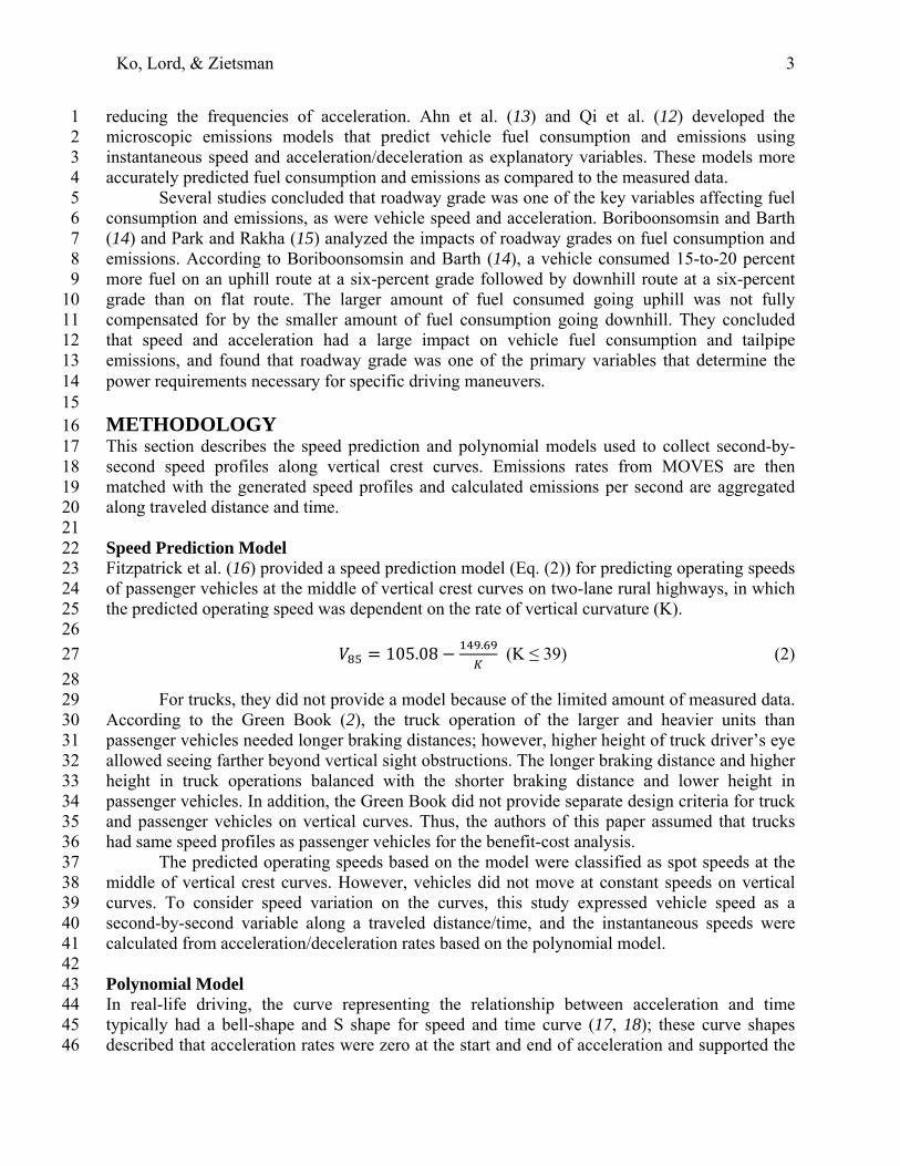
Figure 4 presents the amount of fuel consumption and emissions related to various K-8 values on the curves during a trip by the single-design vehicle. The comparisons were made 9 between increased/decreased K-values and the minimum standard as the base condition. 10 11
(a) Fuel Consumption (b) CO2
(c) NOx (d) CO
(e) HC (f) PM2.5
FIGURE 4 Fuel consumption and emissions by rate of vertical curvature.
0
0.2
0.4
0.6
0.8
1
1.2
0
0.005
0.01
0.015
0.02
0.025
0.03
0.035
0.04
0.5K 0.6K 0.7K 0.8K 0.9K K 1.1K 1.2K 1.3K 1.4K 1.5K
EMF
Fuel Consumption (gal/trip)
Rate of Vertical Curvature (m/%)
Fuel Consumption EMF
0
0.2
0.4
0.6
0.8
1
1.2
0
50
100
150
200
250
300
350
0.5K 0.6K 0.7K 0.8K 0.9K K 1.1K 1.2K 1.3K 1.4K 1.5K
EMF
CO2 (g/trip)
Rate of Vertical Curvature (m/%)
CO2 EMF
0
0.2
0.4
0.6
0.8
1
1.2
0
0.02
0.04
0.06
0.08
0.1
0.12
0.14
0.16
0.5K 0.6K 0.7K 0.8K 0.9K K 1.1K 1.2K 1.3K 1.4K 1.5K
EMF
NOx (g/trip)
Rate of Vertical Curvature (m/%)
NOxEMF
0
0.2
0.4
0.6
0.8
1
1.2
1.4
0
0.5
1
1.5
2
2.5
3
3.5
0.5K 0.6K 0.7K 0.8K 0.9K K 1.1K 1.2K 1.3K 1.4K 1.5K
EMF
CO (g/trip)
Rate of Vertical Curvature (m/%)
CO
EMF
0
0.2
0.4
0.6
0.8
1
1.2
0
0.005
0.01
0.015
0.02
0.025
0.03
0.5K 0.6K 0.7K 0.8K 0.9K K 1.1K 1.2K 1.3K 1.4K 1.5K
EMF
HC (g/trip)
Rate of Vertical Curvature (m/%)
HCEMF
0
0.2
0.4
0.6
0.8
1
1.2
0
0.001
0.002
0.003
0.004
0.005
0.006
0.5K 0.6K 0.7K 0.8K 0.9K K 1.1K 1.2K 1.3K 1.4K 1.5K
EMF
PM2.5 (g/trip)
Rate of Vertical Curvature (m/%)
PM2.5 EMF

Ko, Lord, & Zietsman 13
1 As K increased, the fuel consumption decreased while traveling on the curves. The design 2 vehicle respectively consumed and produced about 10 percent less fuel and CO2 on the curve 3 designed with a 50-percent increased K (i.e., 59 m/percent) than the minimum standard (i.e., 39 4 m/percent). However, 10 percent more fuel and CO2 were consumed and produced on a 50-5 percent reduced K (i.e., 20 m/percent). Additionally, the vehicle produced 12 percent more NOx 6 and PM2.5 on the curve of a 50-percent reduced K, and 15 percent less NOx and PM2.5 on a 50-7 percent increased K. Especially, for CO and HC emissions, the impacts of the K changes were 8 greater than on other emissions. The vehicle produced CO and HC by 25 percent and 14 percent 9 more for a 50-percent reduced K and 31 percent and 20 percent less for a 50-percent increased K, 10 respectively. 11 12 APPLICATION ON HIGHWAY GEOMETRIC FIELD DATA 13 The previous section quantified the changes in fuel consumption and emissions related to various 14 highway geometric design conditions on the vertical crest curves. To reflect actual design 15 conditions, this section presents an evaluation of fuel consumption and emissions using highway 16 geometric field data collected. In addition, this section provides environmental outputs between 17 actual design conditions and alternatives in terms of benefits and costs, which could be 18 incorporated into the design process. 19 20 Highway Geometric Field Data 21 This study selected actual geometric data on U.S. Route 101 (US 101) in Jefferson County, 22 Washington. Most segments of US101 were defined as a two-lane rural principal arterial. The 23 available geometric data were retrieved from the Washington Department of Transportation 24 websites (WSDOT) and the Highway Safety Information System. 25
Among 970 vertical crest curves identified on US 101, about 15 percent (i.e., 143 curves) 26 were built with less than half of the minimum standard K-values in the Green Book (2). In 27 addition, 502 vertical crest curves, accounting for about 52 percent of total curves, were built 28 with greater than 1.5 times the minimum standards. To apply an environmental evaluation on 29 vertical crest curves, this study identified eight curves with the following features: 30 31
greater than 1.5 times of the minimum standard K-value; 32 greater than 48 km/h design speed; 33 greater or equal to 152 m length of vertical curve (L); and 34 greater than 10 percent of algebraic difference of approach and departure tangent 35
grades (G2- G1). 36 37
Table 2 shows the characteristics of selected curves. 38

Ko, Lord, & Zietsman 14
TABLE 2 Characteristics of Analyzed Vertical Crest Curves on US 101 1
Case Design Speed (km/h)
G1 (%)
G2 (%)
Actual Minimum Design Category L
(m) K
(m/%)L
(m) K
(m/%) 1 64 6.49 -6.60 366 28 176 13 Above-design 2 48 6.50 -6.50 152 12 75 6 Above-design 3 56 5.00 -5.01 169 17 88 9 Above-design 4 64 5.47 -6.04 305 27 154 13 Above-design 5 64 5.00 -5.60 305 29 142 13 Above-design 6 48 5.90 -6.57 152 12 72 6 Above-design 7 64 6.50 -6.51 366 28 174 13 Above-design 8 56 5.00 -6.00 213 20 97 9 Above-design
NOTE: G1= approach tangent grade; G2=departure tangent grade. 2 3
Based on Table 2, the speed profiles were generated for both the actual geometric 4 conditions (i.e., the above-minimum standards) and alternative design conditions with the 5 minimum standards in the Green Book (2). Those speed profiles, in turn, were matched with the 6 fuel consumption and emissions rates in terms of the 23 operating mode bins. Table 3 provides 7 the EMFs comparing the actual conditions with the alternative conditions. In general, the ratios 8 were less than one, meaning that the above-designed curves saved fuel to be consumed and 9 reduced emissions produced (as expected). About four-to-10 percent of fuel consumption and up 10 to 16 percent of emissions were reduced in the selected actual vertical curves, relative to the 11 curves that were designed with the minimum standard K-values. 12
13 TABLE 3 EMFs of Fuel Consumption and Emissions for Selected Vertical Curves 14
Case Fuel
Consumption CO2 NOx CO HC PM2.5
1 0.93 0.93 0.90 0.92 0.92 0.93 2 0.95 0.95 0.92 0.94 0.94 0.97 3 0.93 0.93 0.91 0.93 0.93 0.94 4 0.95 0.95 0.93 0.95 0.95 0.95 5 0.90 0.88 0.88 0.84 0.87 0.87 6 0.96 0.96 0.96 0.96 0.96 0.96 7 0.93 0.93 0.90 0.92 0.92 0.93 8 0.94 0.94 0.91 0.93 0.94 0.97
15 The primary reason for fuel savings and emissions reductions for the above-designed 16
curves could be explained by the length of vertical curve. Higher K-values created longer length 17 of the vertical curves and provided more gradual flattening changes on the curvature. This 18 gradual flattening, in turn, could reduce vehicle engine loads on the curves. The reduced demand 19 on the engine power led to less fuel usage and less pollution. 20 21
Ko, Lord, & Zietsman 15
Benefit-Cost Analysis 1 For the vertical curves used in the previous section, the authors conducted a benefit-cost analysis 2 between the curves designed with the actual K-values and the minimum standards. For reference, 3 the environmental evaluation process, same as the passenger car, was applied for the trucks, and 4 both vehicles did not have speed reduction on the curves with greater than or equal to the 5 minimum standard K-values. When a vertical curve was designed with the above minimum 6 standards, it caused additional earthwork because of the flattening curvature design. The 7 earthwork volumes were determined using the average area method under the assumptions that 8 the width of a two-lane highway was nine meter and the cut side slopes were 2:1. Additional 9 construction costs for the earthwork were estimated with the amount of volumes and unit price 10 (i.e., one cubic meter earthwork equals $9.4 (20)). 11
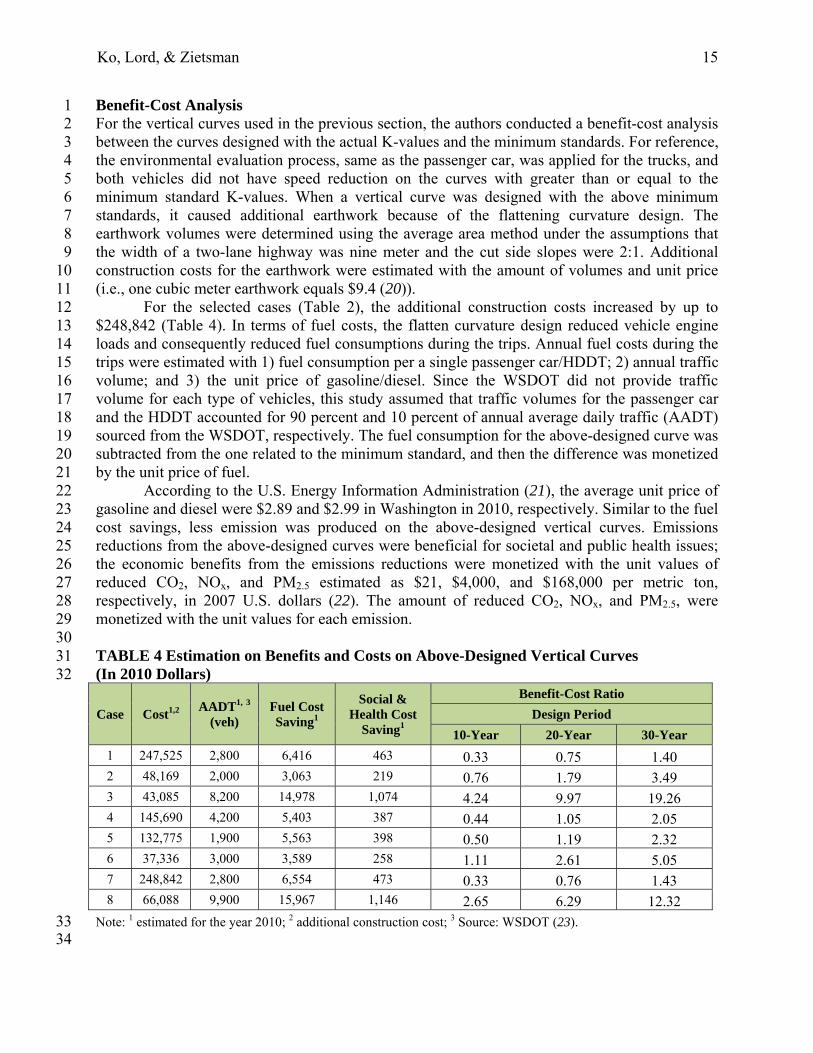
For the selected cases (Table 2), the additional construction costs increased by up to 12 $248,842 (Table 4). In terms of fuel costs, the flatten curvature design reduced vehicle engine 13 loads and consequently reduced fuel consumptions during the trips. Annual fuel costs during the 14 trips were estimated with 1) fuel consumption per a single passenger car/HDDT; 2) annual traffic 15 volume; and 3) the unit price of gasoline/diesel. Since the WSDOT did not provide traffic 16 volume for each type of vehicles, this study assumed that traffic volumes for the passenger car 17 and the HDDT accounted for 90 percent and 10 percent of annual average daily traffic (AADT) 18 sourced from the WSDOT, respectively. The fuel consumption for the above-designed curve was 19 subtracted from the one related to the minimum standard, and then the difference was monetized 20 by the unit price of fuel. 21
According to the U.S. Energy Information Administration (21), the average unit price of 22 gasoline and diesel were $2.89 and $2.99 in Washington in 2010, respectively. Similar to the fuel 23 cost savings, less emission was produced on the above-designed vertical curves. Emissions 24 reductions from the above-designed curves were beneficial for societal and public health issues; 25 the economic benefits from the emissions reductions were monetized with the unit values of 26 reduced CO2, NOx, and PM2.5 estimated as $21, $4,000, and $168,000 per metric ton, 27 respectively, in 2007 U.S. dollars (22). The amount of reduced CO2, NOx, and PM2.5, were 28 monetized with the unit values for each emission. 29 30 TABLE 4 Estimation on Benefits and Costs on Above-Designed Vertical Curves 31 (In 2010 Dollars) 32
Case Cost1,2 AADT1, 3
(veh) Fuel Cost Saving1
Social & Health Cost
Saving1
Benefit-Cost Ratio
Design Period
10-Year 20-Year 30-Year
1 247,525 2,800 6,416 463 0.33 0.75 1.40
2 48,169 2,000 3,063 219 0.76 1.79 3.49
3 43,085 8,200 14,978 1,074 4.24 9.97 19.26
4 145,690 4,200 5,403 387 0.44 1.05 2.05
5 132,775 1,900 5,563 398 0.50 1.19 2.32
6 37,336 3,000 3,589 258 1.11 2.61 5.05
7 248,842 2,800 6,554 473 0.33 0.76 1.43
8 66,088 9,900 15,967 1,146 2.65 6.29 12.32
Note: 1 estimated for the year 2010; 2 additional construction cost; 3 Source: WSDOT (23). 33 34

Ko, Lord, & Zietsman 16
Finally, Table 4 shows the reduced costs (i.e., benefits) from the fuel consumption and 1 societal and health categories and the increased construction costs. Additionally, the expected 2 benefits and costs during 10-year, 20-year, and 30-year design periods were adjusted to 2010 3 dollars with a three-percent discount rate for the social and health costs and a seven-percent 4 discount rate for the fuel costs (24). In Case 3, the benefits due to the flattening curve design 5 exceeded the cost for a 10-year design period; the benefits were greater than four times of the 6 cost. Furthermore, about 19 times more benefits relative to the cost were expected for a 30-year 7 design period. In 30 years after a highway construction or improvement project, benefits were 8 greater than the costs for all cases. 9 10 DISCUSSION AND CONCLUSIONS 11 There were two key factors that affected fuel consumption and emissions during the trips on 12 vertical crest curves – speed and grade variation resulting from the rate of vertical curvature. 13 According to the speed prediction model, the operating speed in the middle of the vertical crest 14 curve was reduced by the K-value. However, this research did not find an important reduction in 15 speed in the middle of the curve under the scenarios evaluated. Less than 3 km/h speed reduction 16 was found on the curves designed with only the 50-percent and 40-percent reduced K-values. 17 Alternately, deceleration and acceleration did not have a great impact on environmental analyses 18 because there was little difference between approaching tangent speeds and operating speeds on 19 the curves. Rather than the K-value influencing the speed reduction, the grade adjustment by the 20 K-value actually affected environmental analyses. 21
Greater K values allowed for longer vertical curvature length, and the longer length 22 allowed for gradual flattening grade changing (Figure 2 (a)). As a result, the design vehicle 23 respectively consumed and produced 10 percent less fuel and CO2. For other emissions analyzed, 24 there were also reductions by up to 31 percent. Lower grade changes resulted in reduced fuel 25 consumption and emissions production from the trip on the vertical crest curve. In addition, from 26 the application of environmental analysis on the selected actual vertical curves, this study 27 showed that the actual vertical curve designed with greater K-values (the above-design) reduced 28 fuel consumption and emissions by up to 16 percent, and the monetized benefits exceeded the 29 additional construction costs for a 30-year design period for all selected cases. Although this 30 paper did not provide the results with various truck proportions, the benefits increased with 31 higher truck proportions (7). 32
In conclusion, a vertical curve should be designed so that the rate of vertical curvature is 33 greater than or at least equal to the minimum standards in design handbooks. A design allowing 34 the curve to be flatter reduces vehicle engine loads and results in less fuel consumption and 35 lower emissions production on the curve. 36
From the quantified results of fuel consumption and emissions related to various 37 conditions on the vertical crest curves, this paper provides the guidelines and tools to quantify 38 environmental impacts that highway designers and engineers can use as part of the highway 39 design process; an application on other geometric components will be covered elsewhere. For the 40 vertical curve design, the guidelines and tools proposed in this paper can reduce the uncertainty 41 associated with the engineering judgment for environmentally-friendly highway design. Finally, 42 this paper shows that adverse environmental impacts from vehicle movements on the curve can 43 be controlled and reduced throughout environmentally conscious highway design. 44
However, the results provided in this paper are dependent on the assumptions on the 45 design vehicle characteristics, fuel type, weather condition, and/or truck proportion of total 46
Ko, Lord, & Zietsman 17
traffic volume. The results should not be taken at face-value and should not be used for decision-1 making purposes. In addition, additional fuel consumption and emissions due to the construction 2 for the flattening curvatures were not considered in the benefit-cost analysis. As future research, 3 a systematic tool predicting fuel consumption and emissions merely by inputting selected design 4 conditions into the system will be beneficial; highway designers and engineers can predict the 5 environmental impact based on the selected design conditions and compare that impact with 6 other design conditions without any complex calculation and repetitive processing used in this 7 study. 8 9 REFERENCES 10 1. U.S. House of Representatives Committee on Science and Technology, 2008. Sustainable, 11
Energy Efficient Transportation Infrastructure. Science and Technology, Washington, D.C. 12 www.democrats.science.house.gov/Media/File/Commdocs/hearings/2008/Tech/24june/Heari13 ng _Charter.pdf, accessed August 11, 2010. 14
15 2. AASHTO. Green Book - A Policy on Geometric Design of Highways and Streets (5th 16
Edition). American Association of State and Highway Transportation Officials, Washington, 17 D.C., 2004. 18
19 3. FHWA. Key Highway Geometric Design Features. Federal Highway Administration, 20
Washington, D.C. www.fhwa.dot.gov/ design/t504028.cfm, accessed November 2010. 21 22 4. TxDOT. Roadway Design Manual. Texas Department of Transportation, Austin, Texas, 23
2010. 24 25 5. AASHTO. Highway Safety Manual. American Association of State and Highway 26
Transportation Officials, Washington, D.C., 2011. 27 28 6. Bonneson, J., K. Zimmerman, and K. Fitzpatrick. Interim Roadway Safety Design Workbook. 29
Publication FHWA/TX-06/0-4703-P4. Texas Transportation Institute, The Texas A&M 30 University System, College Station, Texas, 2006. 31 32
7. Ko, M. Incorporating Vehicle Emission Models into the Highway Design Process. Ph.D. 33 Dissertation, Zachry Department of Civil Engineering, Texas A&M University, College 34 Station, Texas, 2011. 35
36 8. Song, G., and L. Yu. "Estimation of Fuel Efficiency of Road Traffic by Characterization of 37
Vehicle-Specific Power and Speed Based on Floating Car Data." In Transportation Research 38 Record: Journal of the Transportation Research Board, No. 2139, Transportation Research 39 Board of the National Academies, Washington, D. C., 2009, pp. 11-20. 40
41 9. Zhai, H., H. C. Frey, and N. M. Rouphail. "A Vehicle Specific Power Approach to Speed- 42
and Facility-Specific Emissions Estimates for Diesel Transit Buses." Environmental Science 43 & Technology, Vol. 42, No. 21, 2008, pp. 7985-7991. 44
45

Ko, Lord, & Zietsman 18
10. Barth, M., and K. Boriboonsomsin. "Real-World Carbon Dioxide Impacts of Traffic 1 Congestion." In Transportation Research Record: Journal of the Transportation Research 2 Board, No. 2058, Transportation Research Board of the National Academies, Washington, D. 3 C., 2008, pp. 163-171. 4
5 11. Servin, O., K. Boriboonsomsin, and M. Barth. "An Energy and Emission Impact Evaluation 6
of Intelligent Speed Adaptation." The IEEE ITSC, 2006. 7 8 12. Qi, Y. G., H. H. Teng, and L. Yu. "Microscale Emission Models Incorporating Acceleration 9
and Deceleration." Journal of Transportation Engineering, Vol. 130, No. 3, 2004, pp. 348-10 359. 11
12 13. Ahn, K., H. Rakha, A. Trani, and M. Van Aerde. "Estimating Vehicle Fuel Consumption and 13
Emissions Based on Instantaneous Speed and Acceleration Levels." Journal of 14 Transportation Engineering, Vol. 128, No. 2, 2002, pp. 182-190. 15
16 14. Boriboonsomsin, K., and M. Barth. "Impacts of Road Grade on Fuel Consumption and 17
Carbon Dioxide Emissions Evidenced by Use of Advanced Navigation Systems." In 18 Transportation Research Record: Journal of the Transportation Research Board, No. 2139, 19 Transportation Research Board of the National Academies, Washington, D. C., 2009, pp. 21-20 30. 21
22 15. Park, S., and H. Rakha. "Energy and Environmental Impacts of Roadway Grades." In 23
Transportation Research Record: Journal of the Transportation Research Board, No. 1987, 24 Transportation Research Board of the National Academies, Washington, D. C., 2006, pp. 25 148-160. 26
27 16. Fitzpatrick, K., and J. M. Collins. "Speed-Profile Model for Two-Lane Rural Highways." In 28
Transportation Research Record: Journal of the Transportation Research Board, No. 1737, 29 Transportation Research Board of the National Academies, Washington, D. C., 2000, pp. 42-30 49. 31
32 17. Akcelik, R., and D. C. Biggs. "Acceleration Profile Models for Vehicles in Road Traffic." 33
Transportation Science, Vol. 21, No. 1, 1987, pp. 36-54. 34 35
18. Wang, J., K. K. Dixon, H. Li, and J. Ogle. "Normal Deceleration Behavior of Passenger 36 Vehicles at Stop Sign-Controlled Intersections Evaluated with In-Vehicle Global Positioning 37 System Data." In Transportation Research Record: Journal of the Transportation Research 38 Board, No. 1937, Transportation Research Board of the National Academies, Washington, D. 39 C., 2005, pp. 120-127. 40
41 19. Akcelik, R., and M. Besley. "Acceleration and Deceleration Models." 23rd Conference of 42
Australian Institute of Transportation Research, Monash University, Melbourne, Australia, 43 2001. 44 45
Ko, Lord, & Zietsman 19
20. Washington Department of Transportation, 2011a. WSDOT Construction Cost Trend. 1 www.wsdot.wa.gov/biz/construction/constructioncosts.cfm, accessed June 20, 2011. 2 3
21. U.S. Energy Information Administration, 2011. Average Fuel Price of Washington in 2010, 4 Washington, D. C. www.eia.gov/dnav/pet/pet_pri_gnd_dcus_nus_a.htm, accessed June 20, 5 2011. 6 7
22. Burris, M. Seattle/LWC Urban Partnership Agreement National Evaluation: Cost Benefit 8 Analysis Test Plan. Texas Transportation Institute, The Texas A&M University System, 9 College Station, Texas, 2011. 10
11 23. Washington Department of Transportation, 2011b. 2010 Annual Traffic Report. 12
www.wsdot.wa.gov/mapsdata/travel/pdf/Annual_Traffic_Report_2010.pdf, accessed June 15, 13 2011. 14 15
24. NHTSA. Final Regulatory Impact Analysis: Corporate Average Fuel Economy for MY 2011 16 Passenger Cars and Light Trucks. Office of Regulatory, Analysis and Evaluation, National 17 Highway Transportation Safety Administration, March 2009. 18