Function-Space Based Solution Scheme for the Size-Modified Poisson-BoltzmannEquation in Full-Potential DFT

Stefan Ringe, Harald Oberhofer,∗ Christoph Hille, and Karsten ReuterChair for Theoretical Chemistry and Catalysis Research Center,

Technische Universitat Munchen, Lichtenbergstr. 4, D-85747 Garching, Germany

Sebastian MateraFachbereich f. Mathematik u. Informatik, Freie Universitat Berlin,

Otto-von-Simson-Str. 19, D-14195 Berlin, Germany(Dated: September 29, 2018)

The size-modified Poisson-Boltzmann (MPB) equation is an efficient implicit solvation modelwhich also captures electrolytic solvent effects. It combines an account of the dielectric solventresponse with a mean-field description of solvated finite-sized ions. We present a general solu-tion scheme for the MPB equation based on a fast function-space oriented Newton method and aGreen’s function preconditioned iterative linear solver. In contrast to popular multi-grid solvers thisapproach allows to fully exploit specialized integration grids and optimized integration schemes.We describe a corresponding numerically efficient implementation for the full-potential density-functional theory (DFT) code FHI-aims. We show that together with an additional Stern layercorrection the DFT+MPB approach can describe the mean activity coefficient of a KCl aqueoussolution over a wide range of concentrations. The high sensitivity of the calculated activity coeffi-cient on the employed ionic parameters thereby suggests to use extensively tabulated experimentalactivity coefficients of salt solutions for a systematic parametrization protocol.

I. INTRODUCTION

In the atomic-scale modelling of (electro-)chemical re-actions on surfaces, clusters or molecules it becomesincreasingly apparent that solvent effects can have aqualitative influence on predicted reaction pathways andrates.[1, 2] This poses a problem especially in first-principles electronic structure approaches where the largenumber of solvent molecules necessary to accurately rep-resent bulk solvent properties render explicit solvationcomputationally impractical. This situation is further ag-gravated when considering non-negligible salt concentra-tions in the solvent. These are known to dramatically in-fluence the electrochemistry,[3, 4] but demand even largersimulation boxes for realistic ionic strengths and correctthermodynamic sampling.

An approximate way to overcome this hurdle is to for-mally integrate out solvent degrees of freedom in orderto treat the solvent outside of a so-called solvation cavityon the level of a dielectric continuum. While there aremany possible choices of such mean-field, implicit solva-tion models[5], regarding the description of ionic effectsPoisson-Boltzmann (PB) theory[6–9] has been remark-ably successful[4, 10–12] and represents a wide-spreadstandard. PB theory also treats the solvated ions onthe level of a mean-field potential.[13] In its original for-mulation it thereby considers only the electrostatic in-teractions between point-like ions in a dielectric mediumto arrive at analytic expressions of appealing simplicity.At this level, PB theory has found application in many

∗ harald.oberhofer@tum.de

fields of molecular modelling, ranging from colloid science[14, 15] and polyelectrolytes[16] over surface science, elec-trochemistry and electrokinetics[4, 17] to the simulationof biological systems[18–20].

Over the years there have been a number of approachesto improve upon the obvious shortcomings of such plainPB theory. These shortcomings comprise e.g. the neglectof short-range steric repulsions between finite-sized ions,the general neglect of ionic correlations and fluctuationsbeyond the mean-field level and the neglect of disper-sive contributions to the interactions. Corresponding at-tempts to improve on these aspects include liquid statetheory approaches[21–25], field theory expansions[26, 27],ion correlation corrections[28, 29], improvements on thedescription of solvent molecules[23, 30, 31] and finite-sizecorrection for the ions[13, 32–39] among a wide varietyof other computational simulation approaches[40–42]. Inthis work we focus on one of the most famous of suchadaptations of PB theory, the size-modified PB (MPB)approach.[13, 32, 35] While maintaining the mathemat-ical and conceptual simplicity of the original PB formu-lation, MPB corrects specifically for finite ion sizes. Forthis, MPB theory makes use of a local excess free en-ergy functional of the ion density[43], which is based ona lattice gas model and corrects for steric ion-ion and ion-solvent repulsions via a blocking of lattice sites.[13] MPBhas proven to yield particularly good results for equally-sized ions and counter-ions with low charges, and is underactive development to this day.[33, 36, 38, 39, 44]

We here present a new methodological approach tosolving the MPB equation (MPBE) that is generalenough to be applied to any kind of system. While inprinciple not tied to any particular electronic structuremethod, we focus on the coupling to density-functional

arX

iv:1

606.

0902

1v1

[co

nd-m

at.m

trl-

sci]

29

Jun

2016

2

theory (DFT). Such a coupling to DFT has recentlybeen achieved for several other implicit solvation mod-els. [5, 45–49] Yet, previous attempts at specificallycoupling DFT and MPB theory either relied on moreapproximate variants of the theory[50, 51] or were lim-ited to specific solvation cavity geometries, such as pla-nar surfaces[52, 53]. More general schemes for arbitrarycavity shapes[54–56] or approaches that can for instanceexploit irregular integration grids are much less commonand subject of current research. Precisely such irregu-lar integration grids are essential, though, in resolvingCoulomb singularities and orbital cusps in all-electronfull-potential formulations of DFT using localized basissets. Our new method is thus specifically geared towardssolving the MPBE in such circumstances by formulat-ing a Newton scheme in function space. Utilizing theproperties of Green’s functions (and multipole expan-sions) for the iterative solution of the linear subproblemsthen yields a self-consistent solvation free energy for arbi-trary cavity shapes. Our approach furthermore includesa model for the well-known Stern layer which separatesthe diffusing ions from the solvation cavity by introduc-ing non-mean-field ion-solute interactions.

This paper is organized as follows: After briefly intro-ducing to MPB theory and deriving a Stern layer cor-rected version of the MPBE, we illustrate the efficientimplementation specifically for the numeric-atomic or-bital (NAO) based DFT framework FHI-aims [57, 58].The fast convergence and high accuracy of the electro-static potential, ion densities and solvation free energiesin electrolyte solutions are then demonstrated for a rangeof neutral, organic molecules taken from the test set in-troduced by Shivakumar et al.[59]. In order to highlightthe capabilities of our methodology we finally evaluatethe concentration-dependent salt activity coefficient ofKCl aqueous solutions and illustrate that the sensitivityof this quantity on the MPB ion parameters offers a novelroute to systematically determine these parameters fromtabulated activity coefficients.

II. THEORY

A. Poisson-Boltzmann Theory

For the sake of self-containment and a consistent no-tation we first provide a brief outline of PB and MPBtheory. In deriving the MPBE and the associated free en-ergy functional we closely followed the work of Borukhovet al.[13] and Tresset[39]. Considered is the purely elec-trostatic interaction of a z : z continuum electrolyte witha solute, which could e.g. be one or more molecules, acluster or a solid surface. The z : z electrolyte of bulk di-electric permittivity εs,bulk hereby contains cations andanions of equal opposite charge, z = z+ = −z−, and

equal bulk ion concentrations, cs,bulk = cs,bulk+ = cs,bulk

− .The total charge distribution of the solute derives from

electronic and nuclear contributions

nsol(r) = nel(r)−∑at

Zatδ(r −Rat)︸ ︷︷ ︸nnuc

, (1)

where the sum ranges over all nuclear centers “at” ofcharge Zat and located at positions Rat. Throughoutthis work we will use atomic units and the typical signconvention known from DFT, so electronic charge densi-ties have a positive sign. This charge distribution givesrise to an electric field E, which causes a displacementfield D in the surrounding dielectric medium. In isotropicmedia this field can be approximated as

D(r) = ε(r)E(r) , (2)

where ε(r) is the position-resolved, static dielectric re-sponse function of the medium[45], i.e. a generaliza-tion of the macroscopic concept of dielectric permittivity,which for instance is 1 in vacuum and ≈ 80 (78.36 in thiswork) in bulk water. In this formulation, all non-localityin the solvent response is neglected, which is valid forsmall enough electric fields causing only a slight varia-tion of the displacement fields.[60]

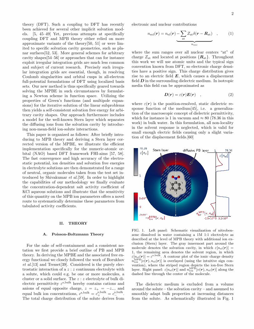
FIG. 1. Left panel: Schematic visualization of nitroben-zene dissolved in water containing a 1M 1:1 electrolyte asdescribed at the level of MPB theory with additional ion ex-clusion (Stern) layer. The gray innermost part around themolecule denotes the solvation cavity, in which ε[nel(r)] =1, the remaining area denotes the solvent region, in whichε[nel(r)] = εs,bulk. A contour plot of the ionic charge densitynMPBion [v(r), nel(r)] is overlayed (using the intuitive sign con-

vention), where the striped region depicts the ion-free Sternlayer. Right panel: ε[nel(r)] and nMPB

ion [v(r), nel(r)] along thedashed line through the center of the molecule.

The dielectric medium is excluded from a volumearound the solute – the solvation cavity – and assumed tosmoothly adapt bulk properties at increasing distancesfrom the solute. As schematically illustrated in Fig. 1

3

this therefore implies ε(r) = 1 within the cavity andε(r) = εs,bulk far away. For the transition in between wespecifically use a parametrization in terms of the electrondensity nel, as it is the finite electron density tails leakingoutside of the cavity that govern the near-solute dielectricproperties in this local formulation. As a monotonousfunction of the electron density, which in turn implic-itly depends on the electrostatic potential v(r), ε(r) thencouples D(r) non-linearly to E(r) at any point in space.The connection between the displacement field and thecharge distribution of the solute is given by the Poissonequation

−∇D(r) = ∇· [ε[nel(r)]∇v(r)] = −4πnsol(r) . (3)

In PB theory the hitherto unaccounted salt ions are intro-duced by simply adding a continuous ionic charge densitynPB

ion(r) to the source term of this Poisson equation. Thisleads to the Poisson-Boltzmann equation

∇ · [ε[nel(r)]∇v(r)] = −4πnsol(r)− 4πnPBion(r) , (4)

with

nPBion(r) = z

[cs+(r)− cs−(r)

], (5)

where cs+(r) and cs−(r) are the spatially-dependent con-centrations of the dissolved cations and anions, respec-tively.

As these ions are mobile and also subject to Coulombinteractions, their distributions depend generally on theoverall electrostatic potential. In a mean-field picture,this dependence would be rigorously captured by thepotential of mean force that would appropriately aver-age over the ionic fluctuations.[12, 60, 61] In PB the-ory this dependence is instead approximately accountedfor through the mean-field electrostatic potential, i.e.cs+(r) = cs+[v(r)], cs−(r) = cs−[v(r)] and correspondingly

also nPBion(r) = nPB

ion[v(r)]. Expressions for these depen-dencies are then e.g. derived from statistical models pa-rameterizing partition functions and minimizing the re-sulting free energy expressions with respect to the elec-trostatic potential (see below).[13]

B. Size-Modified Poisson-Boltzmann theory including Stern-layer correction

The various existing flavors of PB theory differ mainlyin the form considered for the ionic concentrationscs±[v(r)] and their dependence on v(r).[62] In the originalformulation arising from Gouy-Chapman[6, 8] or Debye-Huckel theory[9] point-like and Boltzmann distributedions were assumed. One severe disadvantage of this ap-proach, as pointed out by a number of authors[13, 62]and proven by experiments[63, 64], is the disregard ofthe finite ion sizes which leads even for small ions to anoverestimation of the ionic charge accumulation close tothe solute and therefore to overall erroneous ionic effects,

especially for charged solutes creating high electrostaticpotentials |v(r)| at the cavity surface.

MPB theory, as e.g. derived by Borukhov et al. [13],aims to correct for this by giving the ions an explicit size.Its construction is based on a lattice gas model where sol-vent molecules and ions compete for empty lattice sitesof a cell size a, where each lattice site can only be oc-cupied by one particle at a time. From the partitionfunction of this model system one derives a correction tothe free energy functional due to the entropy of the elec-trolytic system, which depends strongly on the size of thelattice cells and the temperature. Minimizing this func-tional with respect to the electrostatic potential yieldsa modified ionic charge density nMPB

ion (r). Including anadditional Stern-layer correction (vide infra) this densityreads

nionMPB[v(r), nel(r)] = −2zcs,bulkαion[nel(r)]

· sinh(zβv(r))

1− φ0 + φ0αion[nel(r)]cosh (zβv(r)). (6)

Here β = 1/kBT is the inverse temperature, wherekB is the Boltzmann constant, T the temperature, andφ0 = 2a3cs,bulk denotes the volume fraction of lattice cellsoccupied by ions. As also illustrated by the example inFig. 1 and in contrast to standard PB theory (which isrecovered for a = 0), this ion distribution function nowremains bounded even in the limit of very large local elec-trostatic potentials |v(r)|. This comes at the expense ofan additional parameter a that needs to be determinedin the application to real systems, cf. Section V B.

Equation (6) additionally contains a so-called ion ex-clusion function αion(r) = αion[nel(r)] which is notpresent in the original MPB formulation of Borukhovet al. [13]. This function corrects for the shortcomingthat in the original MPB theory ions can in principlestill approach the solute atoms as close as half of thelattice cell length a, and could therefore even lie deepwithin the electron distribution nel(r) of the solute. Inreality, however, the diffusive ion layer lies outside thesolvation cavity and is separated from this by an ex-clusion zone, often called the Stern layer [65]. In thislayer, solvent molecules are oriented around the chargeand sometimes (in the case of overall charged solutes)also ions are directly adsorbed. Yet, most importantly,no diffusive ion distribution exists. The origin of thislayer is partly attributed to ion-charge distribution non-mean-field interactions, as e.g. dispersion or short-rangerepulsion interactions[66], which are not included in theoriginal MPB formulation. In explicitly correcting forthis Stern layer, we thereby follow a reasoning analogousto Jinnouchi et al.[54], who included a short-range ion-solute repulsion operator in the Hamiltonian which Daboet al.[67] expressed as an ion exclusion function. We notethat this stands in contrast to other authors like Otaniet al.[53] who claim the original MPBE to be sufficientto treat size effects or Bostrom et al., who apply an addi-tional repulsion/dispersion operator but use the standardPBE instead of the MPBE[66].

4

For a maximum of generality our implementation al-lows the use of finite-sized ions, while still retaining theeffective correction for the Stern layer (cf. also Harris etal.[68]). The resulting ion exclusion function αion[nel(r)]then restricts the region of finite entropy of the electrolyteto the diffusive part of the system, where both solventmolecules and ions compete for lattice sites. We pointout that similar treatments exist in literature, but are of-ten based on sharp step functions.[52] In contrast and asfurther discussed in Section II E, our exclusion function isset to αion = 0 close to the solute and αion = 1 far away,but with a smoothly modeled transition in between. Sim-ilar to our dielectric model, we choose a parameterizationof αion[nel(r)] in terms of the electron density in orderto capture the repulsion from the solute charge reachingbeyond the cavity.

Regardless of the actual treatment of the ions, bothPBE and MPBE are non-linear partial differential equa-tions. As such, their structure precludes an analytic so-lution for all but the simplest solutes, while at the sametime making them difficult to solve numerically.[69] How-ever, for weak solute potentials – e.g. for neutral solutes– the equations can often be linearized to obtain the fa-mous linearized PBE (LPBE) known mainly from Debye-Huckel theory[9]. For our case of the MPBE, the lin-earized ionic charge density in eq. (5) is given by

nLPBion [v(r), nel(r)] = − 1

4πκ2[nel(r)]v(r) , (7)

which correspondingly leads to a LPBE that is linear inv

L0v(r) =

(∇ · [ε[nel(r)]∇]− κ2[nel(r)]

)v(r)

= −4πnsol(r) . (8)

Here,

κ2[nel(r)] =αion[nel(r)]

1 + φ0(αion[nel(r)]− 1)εs,bulkκ2 , (9)

with the Debye-Huckel parameter

κ =

√8πcs,bulkz2β

εs,bulk. (10)

Equations of the LPBE type are indeed much more con-venient to solve, but due to the limitations on the magni-tude of the electrostatic potential, such as e.g. |v(r)| 25 mV for monovalent ions at room temperature[9, 32,70], not universally applicable. Nevertheless, in Sec-tion III below we will demonstrate how the solution ofLPB type of equations can be used as a stepping stoneto solving the fully non-linear MPBE.

C. Free Energy Functional

Next to the solvent’s influence on the electronic struc-ture of the solute, the main observable of interest in an

implicit solvation scheme is the solvation (or electrolyza-tion) free energy ∆Gsol. It is defined as

∆Gsol = Ω(εs,bulk, cs,bulk, nsol(r))

− Ω(εs,bulk = 1, cs,bulk = 0, nsol(r))

− Ω(εs,bulk, cs,bulk, nsol(r) = 0) , (11)

where Ω(εs,bulk, cs,bulk, nsol(r)) is the free en-

ergy of the solute embedded into a solvent con-nected to reservoir of solvent molecules and ions,Ω(ε

s,bulk = 1, cs,bulk = 0, nsol(r)) the free energy of thesolute in vacuum, and Ω(ε

s,bulk, cs,bulk, nsol(r) = 0) thefree energy of the pure electrolyte. Another similar corequantity is the ion effect on the solvation free energy,defined as

∆∆Gion = ∆Gsol(cs,bulk)−∆Gsol(c

s,bulk = 0) . (12)

In MPB theory the required free energy expres-sions are obtained by minimizing a phenomenolog-ically or field-theoretically derived grand potentialΩmfε,αion

[v(r), cs+(r), cs−(r)] with respect to the potentialand ion distributions.[13] Since this only accounts for themean-field electrostatic interactions within the solventand between solute and solvent, additional terms needto be considered in an extended free energy functionalwhen aiming to use MPB theory in combination with afirst-principles electronic structure approach like DFT.Specifically we therefore consider the following free en-ergy functional and from now on drop all r-dependenciesin the equations for improved legibility

Ωε,αion [v, nel, cs+, c

s−] = T S[nel] + Exc[nel]

+ Ωmfε [v, nel, c

s+, c

s−] + Ωmf

αion[nel, c

s+, c

s−]︸ ︷︷ ︸

Ωmfε,αion

[v,nel,cs+,cs−]

+ Ωnon−mf [nel] . (13)

Here, T S[nel] and Exc[nel] are the usual kinetic energyand exchange-correlation (xc) energy functionals of DFTaccounting for corresponding contributions from the so-lute electrons, respectively. No separate Hartree en-ergy functional is considered. Instead, the mean-fieldelectronic interactions within the solute are appropri-ately included in Ωmf

ε [v, nel, cs+, c

s−] which thus accounts

for all corresponding interactions in solute, electrolyteand between solute and electrolyte. The Stern layercorrection gives rise to an additional mean-field termΩmfαion

[nel, cs+, c

s−] (see below) which we treat jointly with

the regular MPB term as Ωmfε,αion

[v, nel, cs+, c

s−]. Finally,

there are also non-mean-field, non-electrostatic interac-tions between solute and solvent Ωnon−mf [nel].[47, 48]While in principle far from trivial, Andreussi et al. haveshown that solvation free energy contributions arisingfrom Ωnon−mf [nel] can to a good degree of accuracy bemodeled as a linear function of volume and surface of

5

the cavity formed around the solute.[48] As further de-scribed in Section II E below, both can be written as inte-grals over the solute charge density, which is why we con-sider here only a dependence on nel for this term. Whileeq. (13) thus contains a number of interactions beyondregular MPB theory, we stress that further interactionscould still be included. This concerns notably an accountfor the entropies of the solute electrons and nuclei at fi-nite temperatures, or entropic terms arising from the ki-netic energies of solvent molecules and ions [39]. For thetargeted free energy differences (∆Gsol, ∆∆Gion) theseterms are not expected to contribute significantly, whichis why they are neglected here in accordance with mostimplicit solvation methods.[45, 47, 48]

The resulting extended free energy functionalΩε,αion

[v, nel, cs+, c

s−] depends on the electron density,

the electrostatic potential and the ion distributions, andneeds to be minimized with respect to all of them toyield the required free energy expression. The mini-mization with respect to the ion distributions concernsonly the Ωmf

ε,αion[v, nel, c

s+, c

s−]-term and can be done

separately. To describe the energy shift due to theadditional Stern layer ion-solute interaction we relatethe ion exclusion function αion to a repulsion potentialvia αion[nel] = exp(−βvrep) and then obtain a freeenergy functional contribution analogous to the work ofJinnouchi and co-workers[54, 71]. While the physics isthus the same, our motivation to use an exclusion func-tion instead of directly imposing a repulsion potential isthereby mainly based on numerical efficiency arguments.The resulting expression then reads

Ωmfαion

[nel, cs+, c

s−] =

∫dr(cs+ + cs−)vrep

= − 1

β

∫dr(cs+ + cs−) ln(αion[nel]) . (14)

Minimizing Ωmfε,αion

= Ωmfε +Ωmf

αionwith respect to the cs±’s

yields a closed expression for the equilibrium distributionof ions around the solute corresponding to eq. (6), cf.supplementary information (SI). Inserting this into thefunctional leads to

Ωmfε,αion

[v, nel]

=

∫dr

−ε[nel]

8π|∇v|2 + nsolv

− 1

βa3ln

(1 +

φ0

1− φ0αion[nel] cosh(βzv)

),

(15)

with a full derivation provided in the SI.

D. Modified Kohn-Sham equations and minimumfree energy expression

Using eq. (15) the extended free energy functionalΩε,αion

of eq. (13) remains a functional of the electron

density and the electrostatic potential. Minimizationwith respect to the latter yields the MPBE of eqs. (4)and (6). Minimization with respect to the former will– in full analogy to standard Kohn-Sham DFT [72] –lead to modified Kohn-Sham equations that additionallyaccount for the solvent and ion effects on the solute elec-tronic structure. Both MPBE and modified Kohn-Shamequations then have to be solved self-consistently to ob-tain the ground-state electron density, the electrostaticpotential and subsequently the ground-state free energy.

In order to fulfill the orthonormality constraint of thesingle-electron Kohn-Sham states minimization with re-spect to the electron density proceeds in practice via theLagrangian

L[v, nel] = Ωε,αion[v, nel]

+

N∑l=1

N∑k=1

λlk

[∫drψ∗l ψk − δlk

], (16)

with the Lagrange multipliers λlk, and N being the to-tal number of single-particle Kohn-Sham states ψl. Thestationary state of this Lagrange functional with respectto all ψl yields the electronic ground state. If L con-tained only the regular DFT energy functional, this mini-mization would yield the standard Kohn-Sham equations.Due to the additional solvation terms coming from Ωmf

ε,αion

and Ωnon−mf in Ωε,αion[v, nel] additional terms will arise

in these equations. In the following we will thereby con-centrate on the terms arising from Ωmf

ε,αion. The effect

of Ωnon−mf will instead only be treated as a non-self-consistent post-correction of the free energy. The re-sults of Section V A suggest this to imply only a neg-ligible error, while simultaneously allowing to avoid thedemanding computation of second derivatives of the freeenergy functional and avoiding numerical instabilities asobserved by several authors[73].

With this simplification and as derived in the SI theonly additional term to the single-particle Kohn-Sham

Hamiltonian hKS arising from the electron density de-pendence of the dielectric function and the ion exclusionfunction is

δvKS,MPBε,αion

= − 1

8π

∂ε[nel]

∂nel|∇v|2

− φ0

βa3

∂αion[nel]

∂nel

cosh(βzv)

1− φ0 + φ0αion[nel] cosh(βzv).

(17)

Self-consistent solution of the thus modified Kohn-Shamequations together with the MPBE yields the ground-state electron density nel,, the ground-state electrostaticand xc potential v and vxc

, respectively, the ground-state single-particle eigenvalues εl, and the ground-stateeigenstate occupation numbers fl,. Using this the freeenergy is finally obtained as (cf. supplementary informa-tion)

6

Ω(εs,bulk, cs,bulk, nsol,) =

Nstates∑l=1

fl,εl, −∫

drnel,vxc + Exc[nel,]−

1

2

∫drnel,v +

1

2

∫drnnucv

−∫

drnel,δvKS,MPBε,αion

+

∫dr

−1

2nMPB

ion [v, nel,]v −1

βa3ln

(1 +

φ0

1− φ0αion[nel,] cosh(βzv)

)+ Ωnon−mf [nel,] , (18)

with Nstates being the number of possibly degeneratedsingle-particle Kohn-Sham states ψl. The first linecontains the regular energy contributions known fromDFT, including the exchange-correlation energy Exc, thenuclear-nuclear repulsion energy and double countingcorrection. The latter two are thereby represented bythe last two terms by adding and substracting the in-teraction of the electrons with the external potential toincrease the stability of the energy expression.[57] Thesecond line contains the additional solvation term arisingwithin the Kohn-Sham framework, the third and fourthlines are the free energy contributions from the MPBgrand potential Ωmf

ε,αionand the last line the non-mean-

field contribution Ωnon−mf that we here only treat as apost-correction. The regular DFT contribution is therebyalready written in a way that allows straightforward inte-gration into a full-potential DFT code like FHI-aims[57].

E. Cavity definition and non-mean-fieldcontributions

For its application, the derived MPB solvation modelrequires functional forms for the dielectric and ion ex-clusion functions, ε[nel] and αion[nel], respectively. Thetransition of both functions from the bulk solution valueto the value inside the solute defines the solvation cavity:ε[nel] for the solvent and αion[nel] the additional Sternlayer for the ions. In principle, the corresponding transi-tion of both physical counterparts, the spatially resolvedpermittivity and the ion exclusion function, respectively,are highly solute and solvent dependent. The choice ofsmooth switching functions depending solely on the so-lute electron density has nevertheless generally shownsatisfactory transferability in the prediction of solvationfree energies.[45, 47, 48] For the present first proof-of-concept of our solvation model we therefore simply em-ploy a functional form developed originally by Andreussiet al..[48] Adaptation of this functional form in the im-plementation in FHI-aims is trivial and future work willconcentrate on a systematic evaluation and parametriza-tion of this form in dedicated applications.

The functional form employed for the dielectric func-

tion is a smoothed step function of the form[48]

εnmin,nmax [nel] =

1 nel > nmax,

et(ln(nel)) nmin < nel < nmax ,

εs,bulk nel < nmin

(19)with

t (ln(nel)) =ln(εs,bulk)

2π

[2π

ln(nmax)− ln(nel)

ln(nmax)− ln(nmin)

− sin

(2π

ln(nmax)− ln(nel)

ln(nmax)− ln(nmin)

)]. (20)

This function goes to one for large nel close to the nucleiand switches smoothly to εs,bulk for low nel far away. Thetransition region – i.e. its position and width with respectto the electron density – is controlled by the two param-eters nmin and nmax. The main benefit of this particularfunctional form is that its gradients are exactly zero out-side of the transition region, and also ∇ ln(ε[nel]) thatappears in our developed solution scheme for the MPBE(cf. eqs. (35) and (37) below) is a smooth function.[48]This increases the numerical stability and the conver-gence with respect to the multipole expansion performedin a NAO-based DFT code like FHI-aims (vide infra).

For simplicity the same functional form is also chosenfor the ion exclusion function

αion,nαmin,nαmax

[nel]

=

0 nel > nαmax

1εs,bulk−1

(et(ln(nel)) − 1) nαmin < nel < nαmax .

1 nel < nαmin

(21)

This function depends on separate boundary density pa-rameters, nαmin/max, since the ion exclusion does not a

priori have to show the same density dependence as thepermittivity[68]. Physically, the two transitions shouldbe related though, which is why we define these bound-ary density parameters through a shift dαion

and a scalingparameter ξαion with respect to the parameters of the di-electric transition

nαmin/max

= exp

(amin/max ± (amax − amin)

1− ξαion

2

)(22)

7

with

amin/max

= ln(nmin/max) + (ln(nmin)− ln(nmax)) dαion. (23)

dαion > 0 then corresponds to the inclusion of a Sternlayer or non-diffusive region around the solvation cavityand a lowering (raise) of ξαion to a sharpening (smoothen-ing) of the Stern layer transition.

Finally, the choice of the electron density used inthe definition of both transition functions deserves fur-ther mention. In principle, the evaluation could eitherbe based on the true electron density nel in each self-consistent field (SCF) step of the DFT solver, or it couldbe based on a rigid electron density obtained by meresuperposition of free atom densities. In contrast to otherauthors [52] we hitherto found only a negligible impact ofa fully self-consistent cavity on the SCF convergence aslong as the cavity lies within reasonable distances to thecharge distribution, cf. Fig. 3 below. All calculations inthis work are correspondingly performed using the self-consistent density, through which we are able to modelthe mutual influence of the dielectric function and theelectron density.

The solvation cavity defined through the transitionfunctions also governs the non-mean-field part of the freeenergy functional Ωnon−mf [nel,]. In the differences ofeq. (11) defining ∆Gsol, this non-mean-field part givesrise to a free energy contribution due to the exclusion ofsolvent molecules from the cavity and non-bonded short-range, as well as dispersion interactions

∆Gnon−mfsol = ∆Gcav + ∆Grep + ∆Gdis , (24)

respectively. In this work we employ the effectiveparametrization for these terms suggested by Andreussiet al.[48], which provide these terms as mere functions ofthe “quantum surface” S and the “quantum volume” Vof the solvation cavity

∆Gnon−mfsol = (α+ γ)S + βV , (25)

with γ the surface tension of the solvent. α and β con-stitute additional free parameters of the model. V and Sare hereby defined as

V =

∫drϑ[nel] (26)

and

S =

∫dr

(ϑ

[nel −

∆

2

]− ϑ

[nel +

∆

2

])× |∇nel|

∆

, (27)

with the switching function ϑ defined in terms of thechosen dielectric function

ϑ [nel] =εs,bulk − ε[nel]

εs,bulk − 1. (28)

The finite difference in eq. (27) is numerically evaluatedthrough a finite difference parameter ∆. In the presentwork this parameter is set to a low value of 10−8, withnegligible effect of variations around this value on thereported solvation free energies.

The free parameters (α+γ), β, nmin, nmax determin-ing the solvation cavity and the non-mean-field free en-ergy contribution of solvent-solute interactions were op-timized by Andreussi et al. to give good agreement ofsolvation energies of a large test set of neutral moleculeswith experimental values.[48] In this work their parame-ter values will be used without further optimization, cf.Section V A below. In addition to these parameters ourMPB + Stern layer solvation model contains the ion-specific set of parameters a, dαion

, ξαion. In total the

model depends thus on seven parameters. Defering asystematic optimization of the entire parameter set toa forthcoming publication, we highlight in Section V Bhow the various ion-specific parameters affect the calcu-lated activity coefficient of KCl aqueous solutions. Thisin turn also shows that these parameters may be derivedby fitting to tabulated salt activity coefficients.

III. FUNCTION-SPACE BASED MPBSOLUTION SCHEME

In the following we develop a function-space based so-lution scheme of the MPBE, eqs. (4) and (6), that isadapted to the specificities of a full-potential DFT codelike FHI-aims[57]. FHI-aims expands the Kohn-Shamwavefunctions in highly efficient atom-centered NAO ba-

sis functions of the form ϕat,i(r) =uat,i(rat)

ratYlm(Ωat),

where rat = |r−Rat| and Ωat = (θat, φat) denote the dis-tance and the angular coordinates of point r with respectto the atom “at”, respectively. Ylm(Ωat) are the sphericalharmonics and uat,i(rat) are numerically tabulated andfully flexible radial functions. The resulting real-spaceintegrations are performed on logarithmically-spaced ra-dial grids in order to optimally resolve the Coulomb sin-gularity and orbital cusps close to the atom centers. Thisirregular grid severely hampers solving the MPBE us-ing common multi-grid finite difference or finite elementschemes as used by many PB-DFT schemes[52, 54] due tothe high costs of interpolation onto regular meshes. Butalso the present singularities and cusps in an all-electrontreatment can contribute to higher computational costof the common methods. Regular meshes will requirevery small step sizes and a corresponding large numberof nodes, in order to resolve the regions close to the nu-clei. Unstructures meshes instead will require an a priorigrid generation step, which, for large problems, can eas-ily become the bottleneck. This is further complicated asthe ion exclusion function and the dielectric function varyrapidly close to cavity’s boundary, which itself changesduring the SCF-cycle. In contrast, our function-spacebased solution scheme using multipole representations isspecifically designed for the mentioned radial integration

8

grids. We thereby automatically resolve the rapid vari-ation close to the nuclei and also avoid the interpola-tion between two very different grids. Furthermore, wecan exploit the efficient machinery for operating on mul-tipole representations built-in into FHI-aims. Analyti-cal gradients of the free energy functional with respectto the nuclear coordinates, while not within the scopeof this study, can in principle be expressed in terms ofderivatives of the atom-centered basis functions and themultipole moments of the electrostatic potential.

Referring to the detailed account provided in ref. [57]FHI-aims achieves an efficient solution of the plain Pois-son equation through a regularization of the electro-static potential v by subtraction of a superposition offree-atom electrostatic potentials vfree

at derived from non-spinpolarized spherical free-atom electron densities nfree

el,at

δv = v −∑at

vfreeat = v − vfree . (29)

Both vfreeat and nfree

el,at, as well as nfreeel =

∑at n

freeel,at are

accurately known as cubic spline functions on the denselogarithmic grids. The remaining difference potential δvis both smooth and free of singularities. It is thus conve-niently expanded in multi-center multipole moments[57]

δv =∑at

lmax∑l=0

l∑m=−l

δvat,lm(rat)Ylm(Ωat) , (30)

where lmax is the maximum angular momentum of thetruncated multipole expansion. δvat,lm denote the atom-centered multipole components of the difference poten-tial, that are suitably localized on the integration gridaround atom “at” through a partitioned integration for-malism involving partition functions pat.[57] In generalall numeric integrations in the FHI-aims package are per-formed via such a partitioning. The Poisson equation isfinally solved in this representation by exploiting the an-alytic Laplace expansion of the unscreened Green’s func-tion G0(|r−r′|) = 1

4π|r−r′| in terms of spherical harmon-

ics.

A. Newton solver for the MPBE

The formulation of partial differential equations(PDEs) like the MPBE in a function-space oriented so-lution approach is nowadays quite common.[74] This ismainly due to the availability of highly efficient solutionschemes, like Newton methods, offering fast quadraticalconvergence.[75] In our implementation we employ such aNewton solver, albeit not based on commonly used finiteelement methods[74], but rather using a multipole basisexpansion which lets us exploit the highly parallel andefficient machinery of FHI-aims without the overhead formesh generation or uniform grids and any additional in-terpolation steps.

As a first step we thus reformulate the MPBE, eqs. (4)and (6), as a functional root-finding problem with respectto v

F [v] = ∇ · [ε∇v] + 4π(nsol + nMPBion [v]) = 0 . (31)

Here and in the remainder of this section we therebydrop the explicit nel-dependence of ε[nel] and αion[nel] inthe equations for clarity, recognizing that for the MPBEsolver only the v-dependence matters. Regularizing v asin eq. (29) the root with respect to the difference poten-tial δv can then be obtained through an iterative Newtonmethod

F ′[vn](δvn+1 − δvn) = −F [vn] , (32)

where F ′ is the Frechet derivative of F , the existence ofwhich is proven in the SI. Inserting F and F ′ yields aLPB-type equation, i.e. a linear PDE in the updateddifference potential δvn+1 (for the derivation see the SI)(

∇ · [ε∇]− h2[vn]

)δvn+1 = −4πεq[vn] (33)

with

h2[vn] = αionαionφ0 − (φ0 − 1) cosh(βzvn)

(1− φ0 + φ0αion cosh(βzvn))2εs,bulkκ2

(34)and a modified source term

−4πεq[vn] = −4π(nel + nMPB

ion [vn]− εnfree)

− ε(∇ ln(ε)) · (∇vfree)− h2[vn]δvn . (35)

Straightforward solution of this LPB-type equation canbe achieved by rewriting it in form of a screened Poissonequation (SPE)(

∆− κ2

)δvn+1 = −4πq[vn] + L1[vn]δvn+1 (36)

with the response operator

L1[vn] = −(∇ ln(ε)) · ∇ −(κ2 − h2[vn]

ε

). (37)

The equations 33 or 36 could in principle be discretizedusing one of the standard techniques, such as finite dif-ferences or finite elements. The resulting linear algebraicsystem needs then to be solved numerically, usually em-ploying an iterative solver. A common prerequisite is asuitable preconditioner for the linear system, which willreduce the number of iteration steps. Here, we insteadfollow a different strategy and perform the precondition-ing directly on the function space level.

In principle, a preconditioner can be regarded as anapproximation to the inverse of the operator definingour linear problem. In eq. (36) the latter is simply

(∆−κ2− L1[vn]), and for (∆−κ2) we know the inverse,

9

which is simply determined by the screened Green’s func-tion G(|r − r′|) = 1

4π|r−r′|e−κ|r−r′|. Using the Green’s

function for preconditioning, we multiply eq. (36) withG(|r − r′|) and integrate over space to arrive at

δvn+1(r) = −∫

dr′G(|r − r′|)(−4πq[vn(r′)]

+ L1[vn(r′)]δvn+1(r′)

), (38)

with surface terms vanishing due to the boundary con-ditions applied on the potential (v → 0 for |r| → ∞).

For the special case L1[vn] = 0 a single evaluation ofthe right hand side of eq. (38) would yield δvn+1 forthe next Newton step from the given vn of the currentNewton step. The integration is performed by expand-ing δvn+1 in multi-center multipoles as further describedin the next subsection. Newton steps are then repeateduntil convergence in δv is reached. In contrast, in the gen-eral case L1[vn] 6= 0, the right hand side of eq. (38) alsodepends on δvn+1, requiring this equation to be solvedself-consistently. For that purpose we perform iterativeintegrations applying our developed multipole expansionrelaxation method (MERM). In this method we apply asimple linear mixing scheme with a mixing parameter ηto the source term −4πq[vn] + L1[vn]δvn+1. Thereby, ateach Newton step we iteratively solve eq. (38) for fixed

q[vn] and L1[vn] until δvn+1 is converged. This con-verged δvn+1 is subsequently used to update q[vn+1] and

L1[vn+1] for the next Newton step defining a new SPEto be solved by the relaxation method. As in the specialcase, Newton steps are then repeated until convergenceof δv is reached.

The multi-center multipole expansion for the integra-tions in eq. (38) is not a prerequisite, but other ap-proaches can also be employed, in particular any solverfor SPEs with fixed right hand sides. Which solver to usecan be decided depending on the available infrastructureof the DFT code at hand. Also the iterative linear solvercould be replaced by more sophisticated schemes suchas Conjugate Gradient[55]. However, we find that theabove approach converges sufficiently fast in all our testsand we do not expect, that the extra amount of CPUload per iteration of higher-level methods will pay off (cf.Section IV B).

As a side note, Andreussi et al. developed a similariterative scheme to solve the Poisson equation for a sol-vent without ions, eq. (3), by their self-consistent contin-uum solvation (SCCS) scheme[48]. When used with fastFourier transforms to solve the SPE instead of multipoleexpansions, our approach formally reduces to the SCCSmethod for ion-free solvents with cs,bulk = 0. In our ab-stract setting, the SCCS can thereby be considered asmaking use of the Poisson equation using the unscreenedG0 as preconditioner instead of the SPE and the screenedG. We find the latter favored when solving the PBE orMPBE, as the SPE then describes exactly the bulk limitfor |r| → ∞, i.e. nMPB

ion → − 14π ε

s,bulkκ2v. This has a ben-

eficial effect on the numerics of the relaxation method aswill be addressed in detail in the following section.

B. Solving the screened Poisson equation viamultipole expansion

The main numerical effort of the derived MPB Newtonsolver lies in solving the SPE by numerical integration ofthe right hand side of eq. (36) via eq. (38). The de-veloped Newton-MERM scheme is generally applicableand computationally efficient approaches to this integra-tion task will depend on the particular code environmentinto which the scheme is incorporated. A basic solverfor SPEs is in fact often already present in diverse DFTcodes[57, 76, 77] in the form of Kerker preconditioners[78]for the electron density. In case of the Kerker pre-conditioner utilized by the NAO-based DFT code FHI-aims[57], the screened Green’s function is first expandedaround the atom centers in terms of spherical harmon-ics similar to the Laplace expansion of the unscreenedGreen’s function [57, 79]

G(|r − r′|) =8κ

4π

∑at,lm

Ylm(Ωat)Y∗lm(Ω′at)

×

kl(κrat)il(κr

′at) for r′at < rat

kl(κr′at)il(κrat) for rat < r′at

, (39)

where il and kl are the modified spherical Bessel andHankel functions, respectively. Inserting this into eq. (38)yields a multi-center multipole expansion of δvn+1 anal-ogous to eq. (30)

δvn+1 =∑at

lmax∑l=0

l∑m=−l

δvat,lm,n+1(rat)Ylm(Ωat) , (40)

with the corresponding multipole moments δvat,lm,n+1

given by radial integrals

δvat,lm,n+1(rat) =

− 8κ

4π

[−4πkl(κrat)

rat∫0

dr′at

il(κr

′at)qat,lm(r′at)

+ kl(κrat)

rat∫0

dr′at

il(κr

′at)L1δvn+1

at,lm

(r′at)

− 4πil(κrat)

∞∫rat

dr′at

kl(κr

′at)qat,lm(r′at)

+ il(κrat)

∞∫rat

dr′at

kl(κr

′at)L1δvn+1

at,lm

(r′at)

],

(41)

where qat,lm andL1δvn+1

at,lm

are the SPE source

term multipole moments obtained by angular integration

10

over the source term itself

−4πqat,lm(rat)

= −4π

∫rat

d2Ωat

pat(r)q[vn]Ylm(Ωat)

(42)

andL1δvn+1

at,lm

(rat)

=

∫rat

d2Ωat

pat(r)

(L1[vn]δvn+1(r)

)Ylm(Ωat)

.

(43)

Numerical evaluation of the radial integral of eq. (41)can then efficiently exploit the internal FHI-aims integra-tion grids. Specifically, we employ a multistep Adams-Moulton integrator[80] and perform an additional inter-polation to an extra-fine logarithmic grid with increasinggrid shell density close to the nuclei. This allows to op-timally resolve the strong variations of δv in the vicinityof the nuclei, but involves only a numerically undemand-ing 1D cubic spline interpolation that is not performancecritical compared to the summation of the multipole mo-ments.

In FHI-aims, the extent of the radial basis functions islimited by an atom-specific confinement potential vcut,at

in order to increase the computational efficiency espe-cially for larger structures.[57] vcut,at smoothly pushesthe atomic components of the charge densities nfree

el,at(rat)to zero between the radii ronset,at and rcut,at, confiningthem spatially to rat < rcut,at. Due to this and the mul-tiplication with the atom-centered partition function pat

in eq. (42), many contributions to the multipole momentsqat,lm(rat) arising from electron density dependencies inq[vn] are also automatically confined. Confined-sourcemultipole moments are beneficial for computational scal-ing with system size and speed.[57] In our approachwe therefore also aim to spatially confine all parts of

qat,lm(rat) andL1δvn+1

at,lm

(rat) arising from other

terms in eqs. (35) and (37). For instance, by choosinga dielectric function of the form of eq. (19) that has azero gradient outside the transition region many terms

in qat,lm(rat) andL1δvn+1

at,lm

(rat) associated with

∇ε terms in eqs. (35) and (37) vanish already after thedielectric transition region, which is usually much closerto the nuclei than ronset,at. The remaining terms coming

from the functions κ2 − h2[vn]ε and

nMPBion [vn]ε yield mul-

tipole moments which become negligibly small alreadybefore ronset,at for all test cases we looked at, but thisdetailed convergence with cutoff radius must, of course,be checked for every individual problem, cf. Section IV B.

The fast decay of the function κ2 − h2[vn]ε is thereby also

the main reason why we recast the Newton method intoa SPE instead of a Poisson equation as e.g. done by An-dreussi et al.[48]. Using a Poisson equation as resolvent

would instead give rise to a term h2[vn]ε in L1[vn]. This

term would take a constant value of κ2 in the bulk sol-

vent, leading to overall unconfinedL1δvn+1

at,lm

(rat)

multipole moments. A similar argumentation motivatedus not to regularize v with the vacuum potential (cf. eq.(29)) as obtained from a solvent-free calculation in FHI-aims as this also leads to unconfined source multipolemoments.

Due to the spatially-confined multipole moments

qat,lm(rat) andL1δvn+1

at,lm

(rat), the explicit radial

integration in eq. (41) is in principle bounded by the cut-off radius. For grid points rat < rcut,at, this means thatthe integration of the third and fourth term in eq. (41)only needs to be carried out up to rcut,at. At grid pointsrat > rcut,at in the far field, the numerical gain is evenmore pronounced. For such points eq. (41) reduces to

δvffat,lm,n+1(rat) =

− 8κ

4π

[−4πkl(κrat)

rcutat∫0

dr′atil(κr′at)qat,lm(r′at)

+ kl(κrat)

rcutat∫0

dr′atil(κr′at)(L1δvn+1

)at,lm

(r′at)

].

(44)

To evaluate δvffat,lm,n+1, we thus need no additional inte-

gration steps in the Adams-Moulton integrator, since theradial integral is independent of rat and therefore fixedfor all rat > rcut,at. Apart from the obvious numericalgain compared to having to run the Adams-Moulton inte-grator over a much larger number of grid points, this alsoimplies that the solution of the SPE and therefore alsoof the MPBE is free of finite integration errors or surfaceintegral terms, since due to the spatially-confined inte-grand all integrations are formally carried out over thewhole space.

Next to these optimized integration routines, the com-putational efficiency of the iterative multipole-expansionscheme can additionally be improved by exploiting thequick decay of high-l multipole moments in the far field.Similar to the regular multipole-based solution of thePoisson equation [57], significant speed-ups and a greatlyimproved scaling of the MPBE solver can in particularbe obtained for large systems by accordingly restrictingthe actual calculation to low-l multipole moments in thefar field. Our implementation of the iterative solver fur-thermore evaluates the angular and radial integrals as-sociated with q[vn] only once at the beginning of eachNewton step. At each iterative step in the MERM thenonly integrals associated to L1[vn]δvn+1 have to be car-

ried out. Due to the spatial confinement of L1[vn]δvn+1

this update is, however, not necessary on the whole in-tegration grid, but instead only on the points whereL1[vn]δvn+1 6= 0. A full update of δvn+1 according toeq. (40) on the entire integration grid is correspondingly

11

only done after the last iterative MERM step. While gen-erally increasing the computational efficiency, this updatestrategy is particularly effective for solvent calculationswithout ions. In this case δvn+1 has to be updated dur-ing the MERM only on the integration grid points of thedielectric transition region and the majority of the inte-gration points close to the nuclei are only considered inthe final update.

C. Solution scheme for the LPBE

The developed multipole-expansion based relaxationmethod (MERM) is generally suited to solve any LPBEs,since all can in principle be rewritten in form of a SPE. Itmay therefore also be applied to solve the actual LPBEgiven in eq. (8). Such a solution could not only be of in-terest for comparison with other PB codes, but also offersa faster alternative to the coupled Newton-MERM solu-tion of the MPBE for cases where the LPBE is a goodapproximation.

We provide the free energy formula for the LPBE casein the SI. The recasting of the LPBE of eq. (8) into aSPE of the form of eq. (36) is analogous to the proceduredescribed in Section III A and leads to a LPB modifiedsource term

−4πεqLPB = −4π(nel − εnfree

el

)− ε (∇ ln (ε)) ·

(∇vfree

)+ κ2vfree (45)

and LPB response operator

LLPB1 = − (∇ ln (ε)) · ∇+

(κ2

ε− κ2

). (46)

In terms of numerical accuracy, qLPB and LLPB1 are

thereby and in contrast to q[vn] and L1[vn] in the New-ton scheme, exactly zero beyond the cutoff radius as longas both ionic and dielectric transitions lie inside the con-finement region.

D. Multipole correction to the total energy

It is well known that the introduction of a multipolebasis for δv leads to a multipole error in the Hartreeenergy.[57] In FHI-aims δv is regularly obtained by solv-ing the Poisson equation using a multipole-expandedδnel = nel − nfree

el . Expressing the multipole error inδnel as δnres

el = δnel − δnmpel ,where δnmp

el is the multipole-expanded regularized electron density and the error in vas vres = v − vmp = δvres, with vmp = vfree+δvmp, whereδvmp is the multipole-expanded regularized electrostaticpotential, we can write the interaction energy between

electrons and electrostatic potential as

1

2

∫drnelv =

∫drnelv

mp

− 1

2

∫dr (nel − δnres

el ) vmp +

∫drδnres

el δvres . (47)

In FHI-aims, the first term is included in the sum overthe eigenvalues in eq. (18) and the second term added asa double counting correction. Neglecting the last term,quadratic convergence in δnres

el can be achieved, as can beseen by expressing δvres as an integral over G0(|r − r′|)and δnres

el .[81]This multipole error will also exist, when the multi-

pole expansion-based MPBE/LPBE solution scheme iscoupled to a DFT code like FHI-aims. The only differ-ence lies in the fact that we do not multipole expandthe electron density itself, but the SPE source term. Wetherefore define the multipole error in the SPE sourceterm, which for the case of the Newton solver is given by

−4πqres +L1δv

res

= −4πq + L1δv + 4πqmp −L1δv

mp

, (48)

where −4πqmp andL1δv

mp

are the multipole-

expanded SPE source functions. Replacing δnresel in

eq. (47) with the error in the SPE source term, this al-lows to write the interaction energy of electron densitywith electrostatic potential as

1

2

∫drnelv =

∫drnelv

mp

− 1

2

∫dr

(nel +

1

4π

(−4πqres +

L1δv

res))vmp

− 1

4π

∫dr(−4πqres +

L1δv

res)δvres . (49)

Expressing δvres in terms of an integral over G(|r − r′|)and −4πqres +

L1δv

res

, one can again confirm the

quadratic convergence of this expression, but this timein the SPE source term multipole error. As required,eq. (49) transfers into eq. (47) for the solvent-free casewith ε ≡ 1 and αMPB

ion ≡ 0 everywhere. Equations forthe implemented LPB solution scheme, cf. Section III C,can be derived analogously by replacing the SPE sourcefunctions accordingly.

IV. DFT + MPB SOLVER IN FHI-AIMS

A. Implementation details

We implemented the Newton-MERM MPB solver intothe full-potential DFT code FHI-aims.[57] Figure 2 illus-trates the basic workflow of this implementation. Theworkflow for the also implemented MERM-based LPBE

12

update

update and

solve SPE via MERM:

no

yesyes

no

modified KS-equation/SCF

solve KS-eq. via eigenvalue solver:

MPBE/Newton

converged? converged?

SPE/MERM

noyesconverged?

FIG. 2. Workflow of the Newton-MERM based MPB solver inside FHI-aims. At each electronic SCF step of FHI-aims theiterative Newton scheme to optimize δv is initiated. Each Newton step then involves the self-consistent solution of the SPE ofeq. (36) through the MERM.

solver is analogous and further described in the SI. FHI-aims solves the modified Kohn-Sham equations contain-ing the additional term δvKS,MPB

ε,αionof eq. (17) through a

SCF cycle. At each corresponding SCF step, i.e. for thethen given nel, the MPBE of eqs. (4) and (6) are solvedwith the Newton-MERM scheme. For this, the itera-tive Newton scheme to optimize δv is initiated, with eachNewton step involving the self-consistent solution of theSPE of eq. (36) through the MERM. Once the SCF cycleis converged, the resulting ground-state electron densityand electrostatic potential are used to evaluate the freeenergy of the solute Ω0 in the presence of solvent andions through eq. (18).

The SCF cycle is initialized with the superposition offree-atom electron densities nfree

el and the superpositionof free-atom potentials vfree. In principle, it could bebeneficial to start solving the MPBE only after a cer-tain number of SCF steps, i.e. avoid the additional costof solving the MPBE in the first SCF steps when theelectron density still changes largely. However, in prac-tice we obtained a faster SCF convergence in fewer stepswhen including the MPBE solver directly from the sec-ond SCF step onwards. To initiate the MPBE solver,ε[nel] and αion[nel] are first evaluated from the nel of thegiven SCF step. At the very first time the MPBE solveris executed,

δv is initialized with the solution of the correspondingLPBE, cf. Section III C, in the case of the MPBE scheme,whereas for LPB calculations, cf. Section III C, we sim-ply set δv = 0. At all later SCF steps, δv is initializedwith the self-consistent δv of the preceding SCF step.The initialized quantities are used to evaluate the SPEsource functions −4πq[vn] and L1[vn]δvn+1 (MPBE) or

−4πqLPB and LLPB1 δv (LPBE), and the resulting SPE

is solved via the MERM until self-consistency in δvn+1

(MPBE) or δv (LPBE) is reached. In case of the MPBEsolver, the updated δvn+1 is then used to update the SPE

source functions, n→ n+1, and restart the MERM untiloverall convergence of δv is reached. With this converged

δv, the Kohn-Sham Hamiltonian hKS is updated and theeigenvalue problem is solved in the next SCF step.

FHI-aims measures the numerical convergence of theelectron density by evaluating the integrated root meansquare change of nel from one SCF step to the next[57]

τSCF =

√∫dr

(δnel,new(r)− δnel,old(r))2

. (50)

In analogy, the convergence of the Newton method andthe MERM is measured through convergence criteriaτNewton and τMERM, respectively, which calculate the cor-responding change in the iteratively optimized potential

τNewton/MERM =

√∫dr

(δvnew(r)− δvold(r))2

.

(51)

B. Numerical convergence

We assess the numerical convergence of the imple-mented DFT-MPB scheme by calculating a test set of13 differently functionalized neutral, organic moleculesdissolved in water containing a 1M 1:1 electrolyte. Thisset constitutes a sub-set of the test set introduced byShivakumar et al.[59] and is described in detail in theSI (cf. Table S1). For all calculations we employ theparametrization of Andreussi et al. for the dielectricfunction (nmin and nmax) and for the non-mean-fieldsolvent-solute interaction part of the solvation energy∆Gnon−mf

sol ((α + γ) and β) as obtained by their bestfit to experimental solvation energies (“fitg03+β”), seebelow.[48] For the ion-specific MPBE parameters repre-sentative values a = 5 A, dαion

= 0.5, ξαion= 1 and

13

T = 300 K are used, cf. Section V B below. GGA-PBE[82] is used as DFT exchange-correlation functional.

5 10 15 20# SCF step

10−8

10−7

10−6

10−5

10−4

10−3

10−2

10−1

τ SC

F

ϵ [nel] ,αMPBion

[nel]

ϵnfree

el

,αMPB

ion

nfree

el

ϵs,bulk ≡ 1, cs,bulk ≡ 0

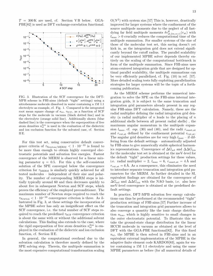
FIG. 3. Illustration of the SCF convergence for the DFT-MPB scheme in FHI-aims (default “tight” settings) using anitrobenzene molecule dissolved in water containing a 1M 1:1electrolyte as example, cf. Fig. 1. Compared is the integratedroot mean square change of nel, τSCF, as a function of SCFsteps for the molecule in vacuum (black dotted line) and inthe electrolyte (orange solid line). Additionally shown (bluedashed line) is the convergence when the superposition of freeatom densities nfree

el is used in the evaluation of the dielectricand ion exclusion function for the solvated case, cf. SectionII E.

For this test set, using conservative default conver-gence criteria of τNewton/MERM < 1 · 10−10 is found tobe more than enough to obtain highly converged elec-trostatic potentials and solvation free energies. Fastestconvergence of the MERM is observed for a linear mix-ing parameter η = 0.5. For this η the self-consistentsolution of the SPE converged below the convergencecriterion for τMERM is similarly quickly achieved for alltested molecules – independent of their size and polar-ity. The number of corresponding MERM steps is ini-tially typically around 60 and then decreases quickly toabout five in subsequent Newton and SCF steps, whichproves the efficiency of the employed preconditioner. Themaximum number of Newton steps required to reach theτNewton < 1 · 10−10 convergence criterion is three. As il-lustrated in Fig. 3, at these settings the incorporation ofthe MPBE solver has only an insignificant effect on theSCF convergence, i.e. the total number of SCF steps re-quired to reach the predefined τSCF convergence criterionis about the same with or without the additional solventcalculations. This finding also extends to the case, wherethe rigid superposition of free atom densities nfree

el is em-ployed in the evaluation of the dielectric and ion exclusionfunction, cf. Section II E.

In general, the computational overhead due to thesolvation calculation is therefore mostly defined by theSPE solving step. Therein, the multipole summation isthe most expensive computational transformation scaling

O(N2) with system size.[57] This is, however, drasticallyimproved for larger systems where the confinement of thesource multipole moments due to the neglect of all fast-dying far field multipole moments δvff

at,lm,n+1(rat) withlmax > 0 crucially reduces the computational time of themultipole summation. For smaller systems of the size ofthose of the molecular test set, this saving doesn’t yetkick in, as the integration grid does not extend signifi-cantly beyond the cutoff radius. The parallel scalabilityof our implemented MPBE solver depends thereby en-tirely on the scaling of the computational bottleneck inform of the multipole summation. Since FHI-aims usesatom-centered integration grids that are designed for op-timal parallel scalability, the multipole summations canbe very efficiently parallelized, cf. Fig. (10) in ref. [57].More detailed scaling tests fully exploiting parallelizationstrategies for larger systems will be the topic of a forth-coming publication.

As the MERM scheme performs the numerical inte-gration to solve the SPE on the FHI-aims internal inte-gration grids, it is subject to the same truncation andintegration grid parameters already present in any reg-ular FHI-aims DFT calculation. Namely, these are theradial multiplier defining the radial integration grid den-sity (a radial multiplier of n leads to the placing of nadditional shells between all present radial shells) , themaximum angular momentum in the multipole expan-sion lmax, cf. eqs. (30) and (40), and the radii ronset,at

and rcut,at defined by the confinement potential vcut,at.The angular grid densities are for very high lmax – if dif-fering from the default settings – automatically adjustedby FHI-aims to give numerically stable spherical harmon-ics representations. Convergence of ∆Gsol and ∆∆Gion

for the molecular test set is obtained at the meV-level forthe default “tight” production settings for these values,i.e. radial multiplier = 2, lmax = 6, ronset,at = 4 A and

rcut,at = 6 A. As a consequence, this eliminates the needto introduce separate truncation and integration grid pa-rameters for the MERM. As further detailed in the SI,equivalent findings are obtained for the convergence of∆Gsol and ∆∆Gion with the NAO basis, i.e. also heremeV-level convergence is obtained at the predefined de-fault settings.

In practice, DFT-MPB solvation free energy calcula-tions can thus be performed at the recommended “tight”production settings of FHI-aims.[57] Further increase ofthe truncation and integration grid parameters allows toalso converge a quantity like the ionic charge distribu-tion nion, which is highly sensitive to small changes inthe outer electrostatic potential. To illustrate this wetake the ground-state charge distribution for the linearHCCH molecule in vacuum as obtained at the level ofDFT with the GGA-PBE functional[82]. For this fixednel, the MPBE is then solved in FHI-aims and in anequivalent external implementation of the MPBE in theadaptive finite element code KARDOS[83], again for wa-ter containing a 1M 1:1 electrolyte and using the sameMPBE parameters as before (for all numerical details of

14

FIG. 4. Comparison of the ionic charge distribution nMPBion

as calculated for HCCH dissolved in water containing a 1M1:1 electrolyte (shown with intuitive sign convention), oncewith the adaptive finite-element code KARDOS (left half)and with the implementation in FHI-aims (right half). TheFHI-aims calculations were performed with the default nu-merical settings lmax = 6 (upper panel) and with a higheraccuracy of the multipole expansion lmax = 8 (lower panel).

the FEM calculations cf. supplementary information).Figure 4 compares the corresponding results for ioniccharge density nMPB

ion obtained by by both methods. Theleft panel shows the results from a highly accurate FEMbenchmark calculation, while the upper right panel showsthe results from FHI-aims calculation using lmax = 6 (de-fault “tight” settings) and the lower right panel usinglmax = 8. As can be seen, qualitative agreement of theion density is already achieved at FHI-aims productionsettings. The residual error in the electrostatic potentialwhich we showed to be negligably small on an energyscale (see above) is further reduced by increasing the or-der of the multipole expansion. Changing to a chargedmolecule, we even get excellent agreement for the dif-ference of ionic charge densities nMPB

ion − nLPBion which is

particularly challenging to resolve and a correspondingplot is shown in the supplementary information.

V. PERFORMANCE ANDPARAMETRIZATION

A. Solvation free energies of neutral molecules

Like any other implicit solvation method also MPBis an effective approach. Its capabilities and reliabil-ity therefore stand and fall with its parametrization.As stated before, our Stern-layer corrected MPB model

builds on a total of seven free parameters. These are,on one hand, the two parameters nmin, nmax definingthe solvation cavity and the two parameters (α+ γ), βgoverning the non-mean-field free energy contribution∆Gnon−mf

sol . On the other hand, there are the three ion-specific parameters a, dαion , ξαion describing the finiteion size and the Stern layer. The latter group of pa-rameters does obviously not enter for ion-free solvents.Aspiring a transferable parameter set that holds for awide range of systems and conditions, this suggests toseparately determine and optimize the prior non-ionicparameter group through solvation calculations for ion-free solvents.

This strategy has been pursued by Andreussi et al.for their SCCS scheme [48], to which our MPB +Stern correction scheme reduces formally for ion-free sol-vents. They optimized the four parameters by fittingto the experimental solvation free energies of the 240-molecule test set of Shivakumar et al.[59] to obtain the“fitg03+β” parameter set: nmin = 0.0001, nmax = 0.005,α + γ = 50 dyn/cm, β = −0.35 GPa. Similarly, they ar-rived at optimized parameter sets for charged solutes,i.e. the “fit cations” (nmin = 0.0002, nmax = 0.0035,α + γ = 5 dyn/cm, β = 0.125 GPa) and the “fit an-ions” (nmin = 0.0024, nmax = 0.0155, α + γ = 0, β =0.450 GPa) parameter sets. Figure 5 reproduces theirpublished solvation free energies ∆Gsol(c

s,bulk = 0) ob-tained with the “fitg03+β” set for the neutral moleculetest set and compares to the corresponding results ob-tained with our implementation and the same parameterset. Specifically we show the deviation with respect tothe experimental reference, and for maximum compara-bility we employ their reference geometries and the sameDFT GGA-PBE functional [82] also used by Andreussi etal.[48]. The agreement between both solvers is excellentwith a mean average error (MAE) of 9.3 meV over thetest set. A large part of this small difference is therebydue to the different basis sets employed in the two DFTcodes, which affect the position of the solvation cavity viathe density cutoffs. Using e.g. a Gaussian aug-cc-pVDZbasis in the FHI-aims implementation indeed reduces theMAE to an insignificant 6.5 meV (cf. supplementary in-formation). We emphasize that we validated that thisremaining deviation has nothing to do with the non-self-consistent evaluation of the ∆Gnon−mf

sol contribution inour implementation as compared to the self-consistentevaluation in the SCCS scheme. For the entire test set,this non-mean-field contributions have a negligible effecton the electron density, justifying the computationally ef-ficient treatment of this contribution as a post-correction.In contrast to other authors completely neglecting thiscontributions[73, 84], we expect our approach in generalto capture the majority of these effects by at the sametime avoiding numerical problems[73].

15

0 50 100

150

200

index

−4

−2

0

2

4

kcal

/mol

∆GSCCSsol − ∆Gexp

sol

∆Gaimssol − ∆Gexp

sol

−200

−100

0

100

200

meV

FIG. 5. Deviations of calculated room-temperature solvation free energies ∆Gsol(cs,bulk = 0) from experimental values for the

Shivakumar test set of 240 neutral molecules [59]. Compared are published results from the SCCS solver of Andreussi et al.[48] with our implementation in FHI-aims (“tight” settings), both using the optimized “fitg03+β” parameter set. The MAEof the present implementation with respect to experiment is 53 meV, the MAE with respect to the SCCS solver is 9.3 meV.

B. Activity coefficient of KCl aqueous solutions

The true potential of the MPB approach unfolds inthe application to electrolyte solutions, where it ac-counts for effects of a finite ion concentration on topof the pure dielectric response of the solvent. For this,three further ion-specific parameters need to be specified,a, dαion , ξαion. Of these three, a describes a finite ionsize within the original size-modified PB approach, whiledαion and ξαion describe the additional ion exclusion in theStern layer. All three will generally sensitively determinethe description of ionic effects [38, 68]. Notwithstanding,to date there is no general parametrization protocol thatwould provide these parameters for a wide range of sys-tems and conditions. Deferring a systematic explorationto a forthcoming publication, we note that activity coef-ficients of electrolyte solutions could represent an inter-esting route to this end. Such coefficients are obviouslya sensitive measure of ionic effects [85–88] and are tabu-lated for a wide range of electrolytes [89, 90]. Fitting tothis experimental reference data would then allow to de-termine the ion-specific MPB parameters, while it wouldsimultaneously provide a first assessment of how well theDFT+MPB+Stern layer approach is capable of treatingsituations with finite ion concentrations.

We illustrate this concept for KCl aqueous solutionsand concentrate on the experimentally well accessiblemean molar activity coefficient[91]

ln(γmean) =1

2

(ln(γ−) + ln(γ+)

), (52)

which averages over anionic and cationic contributions.The activity coefficients of anions, γ−, and cations, γ+,can thereby be expressed as

kBT ln(γ±(cs,bulk)) = µ±(cs,bulk)− µ±(cs,bulk = 0)

= ∆∆G±ion . (53)

Here, µ±(cs,bulk) and µ±(cs,bulk = 0) are the chemical po-tentials of cation/anion in an electrolyte of salt concen-tration cs,bulk and pure solvent, respectively. Since thesechemical potentials represent the free energy change ∂Ω

∂n±

of the electrolyte or pure solvent system induced byadding solute charge density nsol, respectively, the differ-ence of these chemical potentials is just the already intro-duced ion effect on the solvation free energies ∆∆G±ion.As a consequence, γmean for aqueous solutions containinga certain concentration of monovalent ions such as KClcan thus be obtained from two separate DFT-MPB cal-culations for an electrolyzed K+ and a Cl− ion, and therespective two ion-free solvent calculations performed bythe DFT-LPB solver.

Figure 6 shows corresponding results obtained by usinga parameter set of (α+γ), β, nmin, nmax which was op-timized for cationic and anionic solutes differing remark-ably from the neutral solute parameter set especially forcationic solutes.[92] At first, we only tested the option ofa finite ion size by choosing parameters a > 0 and weused a small value for the thickness of the Stern layer, byusing dion = 0.5. Shown is experimental reference data(where we used ms,bulk ≈ cs,bulk for aqueous solutions atroom temperature, where ms,bulk is the molality of thesolution) up to ion concentrations close to the limit ofsaturated solutions (ms,bulk = 4.803 mol/g)[90], as wellas the analytic Debye-Huckel limiting law

ln(γmean(cs,bulk)) = − βz2κ

2εs,bulk

= −1.166M−1/2√cs,bulk , (54)

which is obtained within LPB theory for the purely elec-trostatic interaction of a point-like charge embedded ina homogeneous dielectric medium with point-like ions of

concentration cs,bulk± . Quite clearly, the deviation of the

experimental data from the Debye-Huckel limit cannot beaccounted for solely on the basis of finite size ions. Only

16

0.5 1.0 1.5 2.0pcs,bulk

M1/2

−0.8

−0.7

−0.6

−0.5

−0.4

−0.3

−0.2

−0.1

0.0ln

(γm

ean )

Debye-Huckel limit

experiment

a = 0a = 2 A

a = 4 A

a = 6 A

FIG. 6. Mean molar activity coefficient γmean at room tem-perature as a function of the square root of the ionic bulk con-centration cs,bulk of a KCl aqueous solution. The solid blackline indicates the experimental curve[90], while the dashedblack straight line represents the limit of the Debye-Huckellimiting law. Compared are calculated activity coefficientsusing a range of a values to account for finite size ions. Otherparameters are: “tight” settings, (α + γ), β, nmin, nmaxfrom the “fit cations” and “fit anions” parameter sets [92],dαion = 0.5, ξαion = 1.0.

unphysically large values of a yield a significant deviationof the calculated activity coefficient away from the linearDebye-Huckel dependence, but do then not produce acurvature that matches the experimental data.

This highlights the necessity to consider an addi-tional Stern layer correction in the implicit solvation ap-proach. Figure 7 correspondingly explores the effect ofthe thereby introduced ionic parameters dαion

and ξαion,

which for the present KCl system are identical for theanionic and cationic case. For any significant Stern layerthickness dαion

> 0.5 we here find the results to be ratherinsensitive to the exact value of a, as had also been re-ported by Harris et al [68]. The results shown in Fig. 7are correspondingly obtained for a physically reasonablea = 2. The calculated activity coefficients vary sensi-tively with the chosen (dαion , ξαion)-pair, indicating that agood account of the experimental variation with ion con-centration can be achieved within this two-dimensionalparameter space. The light green curve in Fig. 7 demon-strates this for optimized parameter values dαion = 1.54and ξαion = 0.137 as resulting from a simple Nelder-Meadfit to the experimental reference data. For these parame-ter values the DFT-MPB + Stern layer approach achievesa decent description over a wide range of ionic concentra-tions, even without any further fine-tuning of the otherMPB parameters. For these optimized ionic parameters,the calculated ionic charge density profile nMPB

ion aroundthe central ion shows furthermore a good coincidence ofthe Stern layer onset with the location of the first sol-vation shell as derived from explicit solvation moleculardynamics simulations by Lenart et al. [86], cf. inset in

0.5 1.0 1.5 2.0−0.8

−0.7

−0.6

−0.5

−0.4

−0.3

−0.2

−0.1

0.0

ln(γ

mea

n )

Debye-Huckel limit

experiment

optimized

dαion = 1

dαion = 2

0.10.51.02.0

0.10.51.02.0

0.10.51.02.0

0.10.51.02.0

2.5 3.0 3.5 4.0 4.50.00.51.01.52.02.53.0

nMPBion

radius (A)

KCl

cs,bulk M1/2

gKCl

))

| |

FIG. 7. Same as Fig. 6, but this time exploring the effect ofdifferent choices of the ionic parameters dαion and ξαion de-scribing the Stern layer correction. The four upper red curvesexplore different ξαion values for dαion = 2, the lower bluecurves the same for dαion = 1. The middle light green curve isthe result of an optimum fit to the experimental data achievedfor dαion = 1.54 and ξαion = 0.137. The inset compares theabsolute value of the ionic charge density nMPB

ion obtained forthe latter parameter values with a typical radial distributionfunction gKCl obtained from explicit molecular dynamics forcefield simulations for this system.[86] Other parameters as inFig. 6 with a = 2 A.

Fig. 7. This provides some physical legitimation to theparameters and suggests that fitting to experimental ac-tivity coefficients provides indeed a reasonable route to asystematic parametrization protocol.

VI. SUMMARY AND CONCLUSIONS

We presented a new ansatz to solve the size-modifiedPoisson-Boltzmann equation for the implicit inclusion ofelectrolytic solvation effects into DFT calculations. Themethod differs from earlier MPBE solvers in that it em-ploys (screened) Green’s functions as preconditioner in afunction space setting. Thereby, it can exploit the rou-tines from the DFT code at hand and needs no special-ized grids for the solution of the MPBE. For the show-case implementation into the numeric-atomic orbital full-potential DFT code FHI-aims we demonstrated this bycombining the Newton solver with a multipole expansionrelaxation method that maximally exploits the atom-centered integration grids of this code. For selected testsystems excellent agreement with high-accuracy adap-tive finite element reference calculations was achieved forionic charge densities without the need to significantlyincrease the numerical truncation and integration gridparameters in FHI-aims. Notwithstanding, at presentthe implicit solvation calculations still impose a notice-able overhead for semi-local DFT calculations of mod-estly sized molecules, but for larger system sizes and/or

17

higher-rung functionals this relative cost is increasinglyreduced, also thanks to the efficient exploitation of theparallelized integration routines offered by FHI-aims.

For ion-free solvents the developed MPB model re-duces formally to the self-consistent continuum solvation(SCCS) scheme introduced by Andreussi et al.[48] Weachieve excellent agreement with this scheme for com-puted solvation free energies for the 240 neutral moleculetest set of Shivakumar et al.[59] Use of the optimizedSCCS parameter sets therefore allows to immediately em-ploy our scheme for transferable solvation calculations forion-free solvents. However, the true power of the MPBapproach unfolds, of course, in the application to elec-trolytes. We show that after the inclusion of a Sternlayer correction the MPB approach is capable of describ-ing the activity coefficient of KCl aqueous solutions over awide range of ionic concentrations. The sensitivity of thecalculated coefficient on the ion parameters employed inthe MPB calculation thereby suggests that fitting to ex-tensively tabulated experimental salt activity coefficientscould constitute a powerful and general parametrizationprotocol. We will explore this route in future work to gen-erate an ideally largely transferable parameter set thatenables MPB+Stern layer implicit solvation calculationsfor a wide range of elements and conditions.

VII. ACKNOWLEDGMENTS

The authors gratefully acknowledge support from theSolar Technologies Go Hybrid initiative of the State

of Bavaria and the German Science Foundation DFG(grant no. RE1509/21-1). S.M.’s research is carried outin the framework of Matheon supported by EinsteinFoundation Berlin. We further would like to thankDr. Oliviero Andreussi and Prof. Nicola Marzari forinsightful discussions and access to their solvation testset.

Supporting Information Available

Derivations of the free energy formulas and Kohn-Sham Hamiltonian correction terms both for the MPBEand the LPBE case are provided. In addition, a detaileddescription of the applied Newton method is appendedalong with extensive accuracy and convergence tests ofthe implemented method. This material is available freeof charge via the Internet at http://pubs.acs.org/.

This document is the unedited Authors version ofa Submitted Work that was subsequently accepted forpublication in the Journal of Chemical Theory andComputation, copyright c©American Chemical Societyafter peer review. To access the final edited andpublished work see http://pubs.acs.org/doi/abs/10.1021/acs.jctc.6b00435.

[1] Koper, M. T. M. Chem. Sci. 2013, 4, 2710–2723.[2] Li, Y.-F.; Liu, Z.-P.; Liu, L.; Gao, W. J. Am. Chem. Soc.

2010, 132, 13008–13015.[3] Israelachvili, J. N. Intermolecular and surface forces, 3rd

ed.; Academic press, 2011; pp 291–380.[4] Hunter, R. J. Foundations of Colloid Science; Oxford

University Press: Oxford, 2001; pp 304–402.[5] Tomasi, J.; Mennucci, B.; Cammi, R. Chem. Rev. 2005,

105, 2999–3093.[6] Gouy, G., J. de Physique 1910, 9, 457–468.[7] Gouy, G. Ann. Phys.(Paris) 1917, 7, 129–184.[8] Chapman, D. Philos. Mag. 1913, 25, 475–481.[9] Debye, P.; Huckel, E. Physikalische Zeitschrift 1923, 24,

305–325.[10] Chen, S. W. W.; Honig, B. J. Phys. Chem. B 1997, 101,

9113–9118.[11] Weetman, P.; Goldman, S.; Gray, C. G. J. Phys. Chem.

B 1997, 101, 6073–6078.[12] Fogolari, F.; Brigo, A.; Molinari, H. J. Mol. Recognit.

2002, 15, 377–392.[13] Borukhov, I.; Andelman, D.; Orland, H. Electrochim.

Acta 2000, 46, 221–229.[14] Verwey, E. J. W.; Overbeek, J. T. G. Theory of the Sta-

bility of Lyophobic Colloids; Elsevier: Amsterdam, 1948.[15] Alexander, S.; Chaikin, P. M.; Grant, P.; Morales, G. J.;

Pincus, P.; Hone, D. J. Chem. Phys. 1984, 80, 5776–5781.

[16] Barrat, J. L. and Joanny, J. F., Adv. Chem. Phys. 1996,94, 1–66.

[17] Lyklema, J. Fundamentals of Interface and Colloid Sci-ence,Volume II: Solid-Liquid Interfaces; Academic Press:San Diego, 1995; 3.2–4.11.

[18] Harries, D.; May, S.; Gelbart, W. M.; Ben-Shaul, A. Bio-phys. J. 1998, 75, 159–173.

[19] Borukhov, I.; Andelman, D.; Orland, H. Macromolecules1998, 31, 1665–1671.

[20] Andelman, D. In Structure and Dynamics of Membranes:From Cells to Vesicles; Lipowsky, R., Sackmann, E.,Eds.; Handbook of Biological Physics; North-Holland,1995; Vol. 1; Chapter 12, pp 603–642.

[21] Kjellander, R.; Marcelja, S. J. Chem. Phys. 1985, 82,2122–2135.

[22] Kjellander, R. J. Chem. Phys. 1988, 88, 7129–7137.[23] Blum, L.; Henderson, D. In Fundamentals of Inhomoge-

neous Fluids; Henderson, D., Ed.; Dekker: New York,1992; Chapter 6, pp 239–276.

[24] Levine, S.; Outhwaite, C. W.; Bhuiyan, L. B. J. Elec-troanal. Chem. 1981, 123, 105–119.

[25] Outhwaite, C. W.; Bhuiyan, L. B. J. Chem. Soc., FaradayTrans. II 1983, 79, 707–718.

18

[26] Netz, R. R.; Orland, H. Europhys. Lett. 1999, 45, 726–732.

[27] Netz, R. R.; Orland, H. Euro. Phys. J. E 2000, 1, 203–214.

[28] Lukatsky, D. B.; Safran, S. A. Phys. Rev. E 1999, 60,5848–5857.

[29] Stevens, M. J.; Robbins, M. O. Europhys. Lett. 1990, 12,81–86.

[30] Torrie, G. M.; Patey, G. N. Electrochim. Acta 1991, 36,1669–1675.

[31] Otto, F.; Patey, G. N. Phys. Rev. E 1999, 60, 4416–4422.[32] Borukhov, I.; Andelman, D.; Orland, H. Phys. Rev. Lett.

1997, 79, 435–438.[33] Boschitsch, A. H.; Danilov, P. V. J. Comput. Chem.

2012, 33, 1152–1164.[34] Chaudhry, J. H.; Bond, S. D.; Olson, L. N. J. Sci. Com-

put. 2011, 47, 347–364.[35] Kralj-Iglic, V.; Iglic, A. J. Phys. II 1996, 6, 477–491.[36] Zhou, S.; Wang, Z.; Li, B. Phys. Rev. E 2011, 84,

021901–1–021901–13.[37] Abrashkin, A.; Andelman, D.; Orland, H. Phys. Rev.

Lett. 2007, 99, 077801–1–077801–4.[38] Chu, V. B.; Bai, Y.; Lipfert, J.; Herschlag, D.; Do-

niach, S. Biophys. J. 2007, 93, 3202–3209.[39] Tresset, G. Phys. Rev. E 2008, 78, 061506–1–061506–9.[40] Guldbrand, L.; Jonsson, B.; Wennerstrom, H.; Linse, P.

J. Chem. Phys. 1984, 80, 2221–2228.[41] Kjellander, R.; Akesson, T.; Jonsson, B.; Marcelja, S. J.

Chem. Phys. 1992, 97, 1424–1431.[42] Greberg, H.; Kjellander, R.; Akesson, T. Mol. Phys.

1997, 92, 35–48.[43] Antypov, D.; Barbosa, M. C.; Holm, C. Phys. Rev. E

2005, 71, 061106–1–061106–10.[44] Li, B. Nonlinearity 2009, 22, 811–833.[45] Fattebert, J. L.; Gygi, F. J. Comput. Chem. 2002, 23,

662–666.[46] Fattebert, J. L.; Gygi, F. Int. J. Quant. Chem. 2003, 93,

139–147.[47] Scherlis, D. A.; Fattebert, J. L.; Gygi, F.; Cococ-

cioni, M.; Marzari, N. J. Chem. Phys. 2006, 124, 074103–1–074103–12.

[48] Andreussi, O.; Dabo, I.; Marzari, N. J. Chem. Phys.2012, 136, 064102–1–064102–20.

[49] Kelly, C. P.; Cramer, C. J.; Truhlar, D. G. J. Chem.Theory Comput. 2005, 1, 1133–1152.

[50] Letchworth-Weaver, K.; Arias, T. A. Phys. Rev. B 2012,86, 075140–1–075140–16.

[51] Tannor, D. J.; Marten, B.; Murphy, R.; Friesner, R. A.;Sitkoff, D.; Nicholls, A.; Ringnalda, M.; Goddard, W. A.;Honig, B. J. Am. Chem. Soc. 1994, 116, 11875–11882.

[52] Fang, Y.-H.; Wei, G.-F.; Liu, Z.-P. Cat. Today 2013,202, 98–104.

[53] Otani, M.; Sugino, O. Phys. Rev. B 2006, 73, 115407–1–115407–11.

[54] Jinnouchi, R.; Anderson, A. B. Phys. Rev. B 2008, 77,245417–1–245417–18.

[55] Fisicaro, G.; Genovese, L.; Andreussi, O.; Marzari, N.;Goedecker, S. J. Chem. Phys. 2016, 144, 014103–1–014103–12.

[56] Mathew, K.; Hennig, R. G. 2016, arXiv:1601.03346.arXiv.org ePrint archive. http://arxiv.org/abs/1601.03346 (accessed June 2, 2016).

[57] Blum, V.; Gehrke, R.; Hanke, F.; Havu, P.; Havu, V.;Ren, X.; Reuter, K.; Scheffler, M. Comp. Phys. Comm.

2009, 180, 2175–2196.[58] Ren, X.; Rinke, P.; Blum, V.; Wieferink, J.;

Tkatchenko, A.; Sanfilippo, A.; Reuter, K.; Scheffler, M.New J. Phys. 2012, 14, 053020–1–053020–55.

[59] Shivakumar, D.; Williams, J.; Wu, Y.; Damm, W.; Shel-ley, J.; Sherman, W. J. Chem. Theory Comput. 2010, 6,1509–1519.

[60] Bonthuis, D. J.; Netz, R. R. J. Phys. Chem. B 2013,117, 11397–11413.

[61] Attard, P. In Advances in Chemical Physics; Hender-son, D., Ed.; John Wiley & Sons, Inc.: Hoboken, 1996;pp 1–159.

[62] Grochowski, P.; Trylska, J. Biopolymers 2008, 89, 93–113.

[63] Cervera, J.; Ramirez, P.; Manzanares, J. A.; Mafe, S.Microfluid Nanofluid 2010, 9, 41–53.

[64] Kosmulski, M. Colloid Surface A 1995, 95, 81–100.[65] Stern, O. Z. Elektrochem. Angew. P. 1924, 30, 508–516,

Deutsche Bunsen Gesellschaft, June 1924, Gottingen,Germany.

[66] Bostrom, M.; Tavares, F. W.; Bratko, D.; Ninham, B. W.J. Phys. Chem. B 2005, 109, 24489–24494.

[67] Dabo, I.; Cances, E.; Li, Y. L.; Marzari, N. 2008,arXiv:0901.0096. arXiv.org ePrint archive. http://

arxiv.org/abs/0901.0096 (accessed June 2, 2016).[68] Harris, R. C.; Boschitsch, A. H.; Fenley, M. O. J. Chem.

Phys. 2014, 140, 075102–1–075102–9.[69] Holst, M.; Sajed, F. J. Comput. Chem. 1993, 14, 105–

113.[70] Kilic, M. S.; Bazant, M. Z.; Ajdari, A. Phys. Rev. B

2007, 75, 021502–1–021502–16.[71] Jinnouchi, R.; Kodama, K.; Hatanaka, T.; Morimoto, Y.

Phys. Chem. Chem. Phys. 2011, 13, 21070–21083.[72] Kohn, W.; Sham, L. J. Phys. Rev. 1965, 140, A1133–

A1138.[73] Steinmann, S. N.; Sautet, P. J. Phys. Chem. C 2016,

120, 5619–5623.[74] Holst, M. J.; Saied, F. J. Comput. Chem. 1995, 16, 337–

364.[75] Deuflhard, P. In Newton Methods for Nonlinear Prob-

lems; Bank, R., Graham, R., Stoer, J., Varga, R.,Yserentant, H., Eds.; Springer, 2004.

[76] Hasnip, P. J. and Probert, M. I. J., 2015,arXiv:1503.01420. arXiv.org ePrint archive. http://

arxiv.org/abs/1503.01420 (accessed June 2, 2016).[77] Shiihara, Y.; Kuwazuru, O.; Yoshikawa, N. Model. Simul.

Mater. Sc. 2008, 16, 035004–1–035004–11.[78] Kerker, G. P. Phys. Rev. B 1981, 23, 3082–3084.[79] Boschitsch, A. H.; Fenley, M. O.; Olson, W. K. J. Com-

put. Phys. 1999, 151, 212–241.[80] Abramowitz, M., Stegun, I. A., Eds. Handbook of math-

ematical functions; Dover Publications, Inc.: New York,1970; p 896.

[81] Dunlap, B. I.; Connolly, J. W. D.; Sabin, J. R. J. Chem.Phys. 1979, 71, 3396–3402.

[82] Perdew, J. P.; Burke, K.; Ernzerhof, M. Phys. Rev. Lett.1996, 77, 3865–3868.

[83] Lang, J. Adaptive multilevel solution of nonlinearparabolic PDE systems: theory, algorithm, and applica-tions; Springer Science & Business Media, 2013; Vol. 16.

[84] Lespes, N.; Filhol, J. S. B. J. Chem. Theory Comput.2015, 11, 3375–3382.

[85] Valisko, M.; Boda, D. J. Chem. Phys. 2014, 140, 234508–1–234508–12.

19

[86] Lenart, P. J.; Jusufi, A.; Panagiotopoulos, A. Z. J. Chem.Phys. 2007, 126, 044509–1–044509–7.

[87] Slavchov, R. I. J. Chem. Phys. 2014, 140, 164510–1–164510–12.

[88] Mester, Z.; Panagiotopoulos, A. Z. J. Chem. Phys. 2015,142, 044507–1–044507–10.

[89] Robinson, R. A.; Stokes, R. H. Electrolyte Solutions, 2nded.; Butterworths Publications Limited: New York, 1959;pp 476–509.

[90] Hamer, W. J.; Wu, Y. C. J. Phys. Chem. Ref. Data 1972,1, 1047–1099.

[91] Robinson, R. A.; Stokes, R. H. Electrolyte Solutions, 2nded.; Butterworths Publications Limited: New York, 1959;p 28.

[92] Dupont, C.; Andreussi, O.; Marzari, N. J. Chem. Phys.2013, 139, 214110–1–214110–8.