equilibrium lorenz curve a generalization …faculty.wcas.northwestern.edu/~kmatsu/equilibrium...
TRANSCRIPT

©Kiminori Matsuyama, Equilibrium Lorenz Curve, A Generalization
Page 1 of 43
Endogenous Ranking and Equilibrium Lorenz Curve Across (ex-ante) Identical Countries: A Generalization
By Kiminori Matsuyama Northwestern University
Prepared for
Joint Vienna Macro Seminar Institut für Höhere Studien
September 17, 2013
©Kiminori Matsuyama, Equilibrium Lorenz Curve, A Generalization
Page 2 of 43
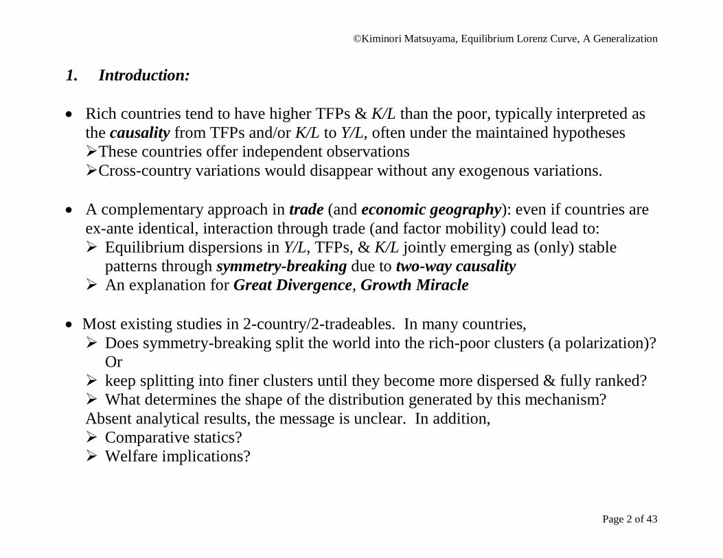
1. Introduction: Rich countries tend to have higher TFPs & K/L than the poor, typically interpreted as
the causality from TFPs and/or K/L to Y/L, often under the maintained hypotheses These countries offer independent observations Cross-country variations would disappear without any exogenous variations.
A complementary approach in trade (and economic geography): even if countries are
ex-ante identical, interaction through trade (and factor mobility) could lead to: Equilibrium dispersions in Y/L, TFPs, & K/L jointly emerging as (only) stable
patterns through symmetry-breaking due to two-way causality An explanation for Great Divergence, Growth Miracle
Most existing studies in 2-country/2-tradeables. In many countries, Does symmetry-breaking split the world into the rich-poor clusters (a polarization)?
Or keep splitting into finer clusters until they become more dispersed & fully ranked? What determines the shape of the distribution generated by this mechanism? Absent analytical results, the message is unclear. In addition, Comparative statics? Welfare implications?
©Kiminori Matsuyama, Equilibrium Lorenz Curve, A Generalization
Page 3 of 43
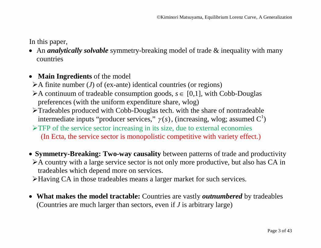
In this paper, An analytically solvable symmetry-breaking model of trade & inequality with many
countries Main Ingredients of the model A finite number (J) of (ex-ante) identical countries (or regions) A continuum of tradeable consumption goods, s [0,1], with Cobb-Douglas
preferences (with the uniform expenditure share, wlog) Tradeables produced with Cobb-Douglas tech. with the share of nontradeable
intermediate inputs “producer services,” )(s , (increasing, wlog; assumed C1) TFP of the service sector increasing in its size, due to external economies
(In Ecta, the service sector is monopolistic competitive with variety effect.) Symmetry-Breaking: Two-way causality between patterns of trade and productivity A country with a large service sector is not only more productive, but also has CA in
tradeables which depend more on services. Having CA in those tradeables means a larger market for such services.
What makes the model tractable: Countries are vastly outnumbered by tradeables
(Countries are much larger than sectors, even if J is arbitrary large)
©Kiminori Matsuyama, Equilibrium Lorenz Curve, A Generalization
Page 4 of 43
1
S3 S2 S1
0
S0 S4
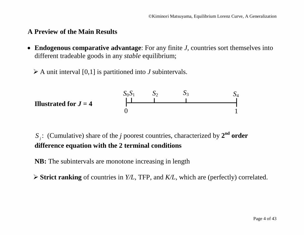
A Preview of the Main Results Endogenous comparative advantage: For any finite J, countries sort themselves into
different tradeable goods in any stable equilibrium; A unit interval [0,1] is partitioned into J subintervals.
Illustrated for J = 4
jS : (Cumulative) share of the j poorest countries, characterized by 2nd order difference equation with the 2 terminal conditions NB: The subintervals are monotone increasing in length
Strict ranking of countries in Y/L, TFP, and K/L, which are (perfectly) correlated.
©Kiminori Matsuyama, Equilibrium Lorenz Curve, A Generalization
Page 5 of 43
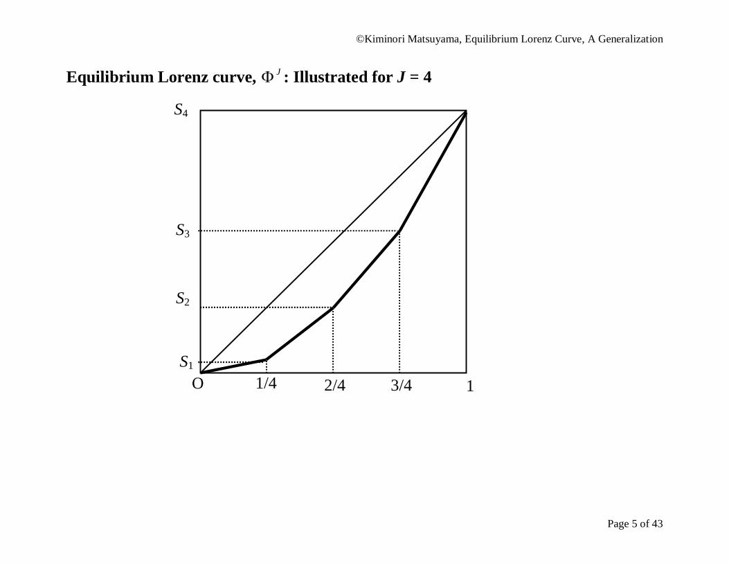
Equilibrium Lorenz curve, J : Illustrated for J = 4
2/4 O
S4
1 3/4 1/4
S3
S2
S1

©Kiminori Matsuyama, Equilibrium Lorenz Curve, A Generalization
Page 6 of 43
As J →∞, the limit Lorenz curve is given by the unique solution of the 2nd order
differential equation with the 2 terminal conditions. Furthermore, analytically solvable.
Shape of Lorenz Curve: conditions for Bimodal distribution (Polarization) Power-law distribution
Comparative Statics:
log-super(sub)modularity Lorenz-dominance Welfare effects of trade: We can also answer questions like; When is trade Pareto-improving? If not Pareto-improving, what fractions of countries would lose from trade?
©Kiminori Matsuyama, Equilibrium Lorenz Curve, A Generalization
Page 7 of 43
Organization of this presentation slides: 1. Introduction 2. Basic Model (Fixed Factor Supply; Without Nontradeable Consumption Goods) Single-country (Autarky) equilibrium (J = 1) Two-country equilibrium (J = 2), not in the paper Multi-country equilibrium (2 ≤ J < ∞) Limit case (J ∞) Polarization Power-law (truncated Pareto) examples Comparative Statics; Log-modularity and Lorenz-dominance
3. Welfare Effects of Trade Multi-country equilibrium (2 ≤ J < ∞) Limit case (J ∞)
4. Formal Stability Analysis, not in the paper 5. Nontradeable Consumption Goods; Effects of Globalization through Goods Trade Multi-country equilibrium (2 ≤ J < ∞) Limit case (J ∞)
6. Variable Factor Supply; Effects of Globalization through Factor Mobility or Skill-Biased Technological Change Multi-country equilibrium (2 ≤ J < ∞) Limit case (J ∞)
7. Concluding Remarks, not in the paper
©Kiminori Matsuyama, Equilibrium Lorenz Curve, A Generalization
Page 8 of 43
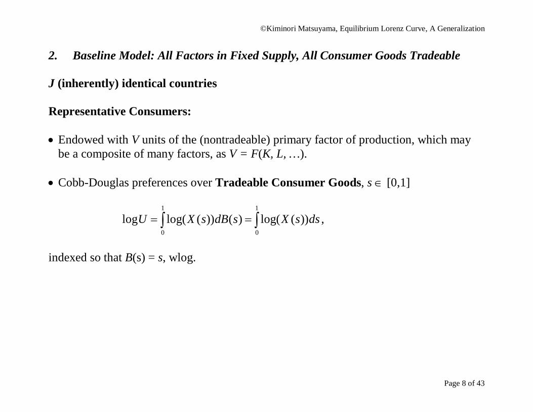
2. Baseline Model: All Factors in Fixed Supply, All Consumer Goods Tradeable J (inherently) identical countries Representative Consumers: Endowed with V units of the (nontradeable) primary factor of production, which may
be a composite of many factors, as V = F(K, L, …).
Cobb-Douglas preferences over Tradeable Consumer Goods, s [0,1]
1
0
1
0
))(log()())(log(log dssXsdBsXU ,
indexed so that B(s) = s, wlog.
©Kiminori Matsuyama, Equilibrium Lorenz Curve, A Generalization
Page 9 of 43
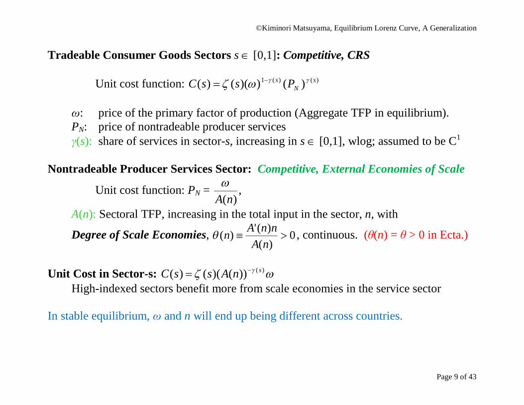
Tradeable Consumer Goods Sectors s [0,1]: Competitive, CRS Unit cost function: )()(1 )())(()( s
Ns PssC
ω: price of the primary factor of production (Aggregate TFP in equilibrium). PN: price of nontradeable producer services γ(s): share of services in sector-s, increasing in s [0,1], wlog; assumed to be C1
Nontradeable Producer Services Sector: Competitive, External Economies of Scale
Unit cost function: PN = )(nA
,
A(n): Sectoral TFP, increasing in the total input in the sector, n, with
Degree of Scale Economies, 0)()(')(
nAnnAn , continuous. (θ(n) = θ > 0 in Ecta.)
Unit Cost in Sector-s: )())()(()( snAssC
High-indexed sectors benefit more from scale economies in the service sector In stable equilibrium, ω and n will end up being different across countries.
©Kiminori Matsuyama, Equilibrium Lorenz Curve, A Generalization
Page 10 of 43
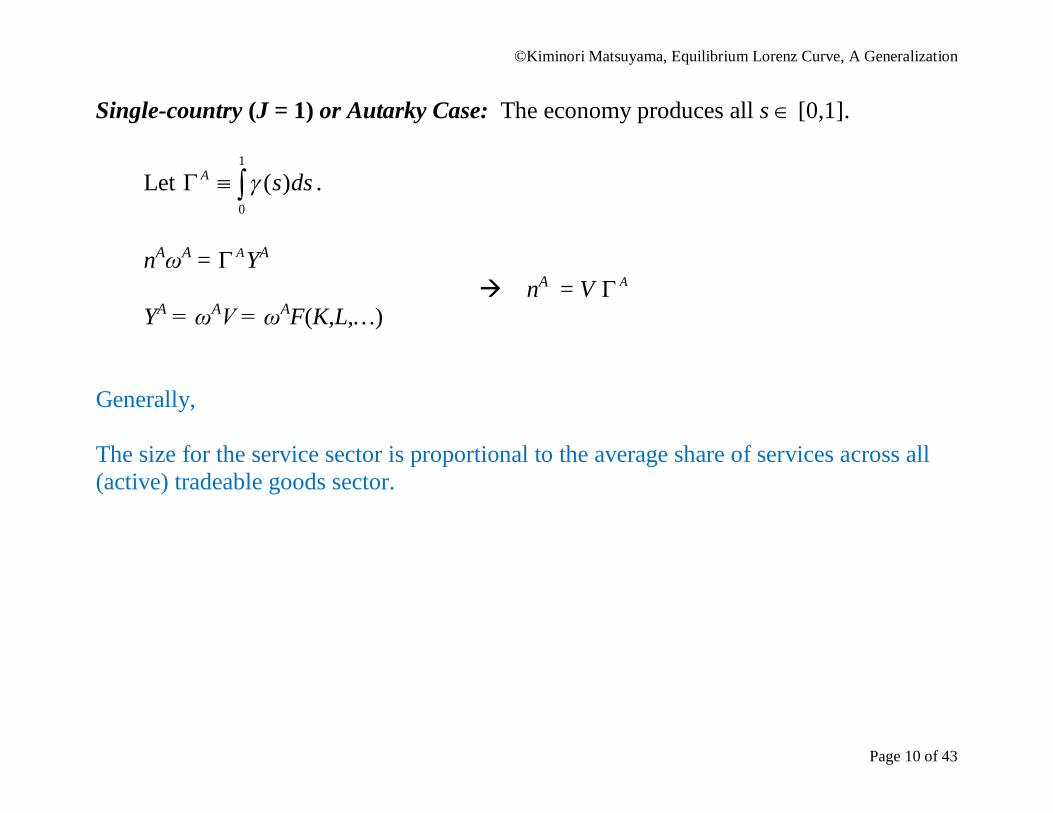
Single-country (J = 1) or Autarky Case: The economy produces all s [0,1].
Let 1
0
)( dssA .
nAωA = A YA
nA = V A YA = ωAV = ωAF(K,L,…)
Generally, The size for the service sector is proportional to the average share of services across all (active) tradeable goods sector.
©Kiminori Matsuyama, Equilibrium Lorenz Curve, A Generalization
Page 11 of 43
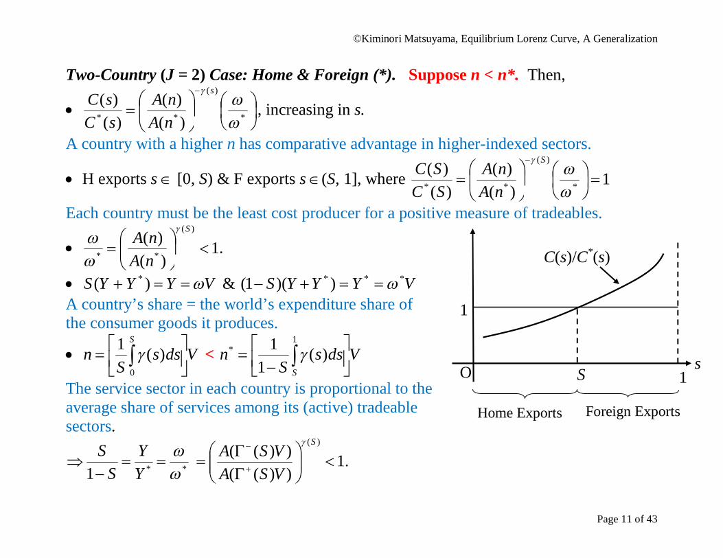
Two-Country (J = 2) Case: Home & Foreign (*). Suppose n < n*. Then,
*
)(
** )()(
)()(
s
nAnA
sCsC , increasing in s.
A country with a higher n has comparative advantage in higher-indexed sectors.
H exports s [0, S) & F exports s (S, 1], where 1)()(
)()(
*
)(
**
S
nAnA
SCSC
Each country must be the least cost producer for a positive measure of tradeables.
1)()(
)(
**
S
nAnA
.
VYYYS )( * & VYYYS *** ))(1( A country’s share = the world’s expenditure share of the consumer goods it produces.
VdssS
nS
0
)(1 < VdssS
nS
1
* )(1
1
The service sector in each country is proportional to the average share of services among its (active) tradeable sectors.
**1
YY
SS 1
))(())((
)(
S
VSAVSA
.
S s 1
Home Exports Foreign Exports
O
1
C(s)/C*(s)
©Kiminori Matsuyama, Equilibrium Lorenz Curve, A Generalization
Page 12 of 43
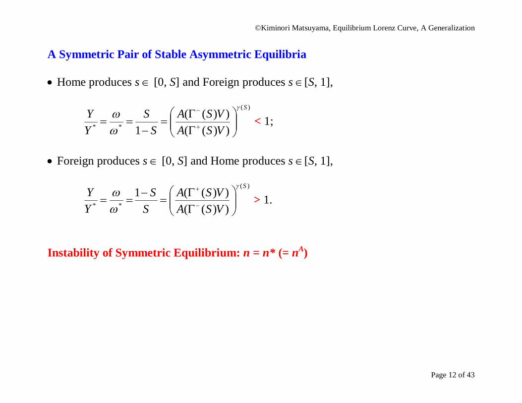
A Symmetric Pair of Stable Asymmetric Equilibria Home produces s [0, S] and Foreign produces s [S, 1],
)(
** ))(())((
1
S
VSAVSA
SS
YY
< 1;
Foreign produces s [0, S] and Home produces s [S, 1],
**
YY
)(
))(())((1
S
VSAVSA
SS
> 1.
Instability of Symmetric Equilibrium: n = n* (= nA)
©Kiminori Matsuyama, Equilibrium Lorenz Curve, A Generalization
Page 13 of 43
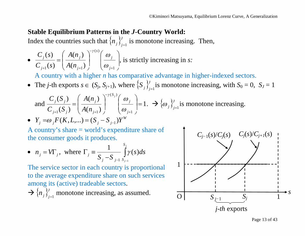
Stable Equilibrium Patterns in the J-Country World: Index the countries such that J
jjn1 is monotone increasing. Then,
1
)(
11 )()(
)()(
j
j
s
j
j
j
j
nAnA
sCsC
, is strictly increasing in s:
A country with a higher n has comparative advantage in higher-indexed sectors. The j-th exports s (Sj, Sj+1), where J
jjS1is monotone increasing, with S0 = 0, SJ = 1
and 1)(
)()(
)(
1
)(
11
j
j
S
j
j
jj
jjj
nAnA
SCSC
. J
jj 1 is monotone increasing.
Wjjjj YSSLKFY )(,...),( 1
A country’s share = world’s expenditure share of the consumer goods it produces.
jj Vn , where
j
j
S
Sjjj dss
SS1
)(1
1
The service sector in each country is proportional to the average expenditure share on such services among its (active) tradeable sectors. J
jjn1 monotone increasing, as assumed. S j−1
s
1
Cj−1(s)/Cj(s) Cj(s)/Cj+1(s)
Sj
j-th exports
1 O
©Kiminori Matsuyama, Equilibrium Lorenz Curve, A Generalization
Page 14 of 43
1
S3 S2 S1
0
S0 S4
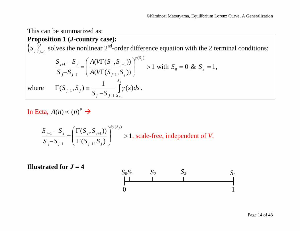
This can be summarized as: Proposition 1 (J-country case): J
jjS0 solves the nonlinear 2nd-order difference equation with the 2 terminal conditions:
1)),(()),((
)(
1
1
1
1
jS
jj
jj
jj
jj
SSVASSVA
SSSS
with 00 S & 1JS ,
where
j
j
S
Sjjjj dss
SSSS
1
)(1),(1
1 .
In Ecta, )()( nnA
1),()),(
)(
1
1
1
1
jS
jj
jj
jj
jj
SSSS
SSSS
, scale-free, independent of V.
Illustrated for J = 4
©Kiminori Matsuyama, Equilibrium Lorenz Curve, A Generalization
Page 15 of 43
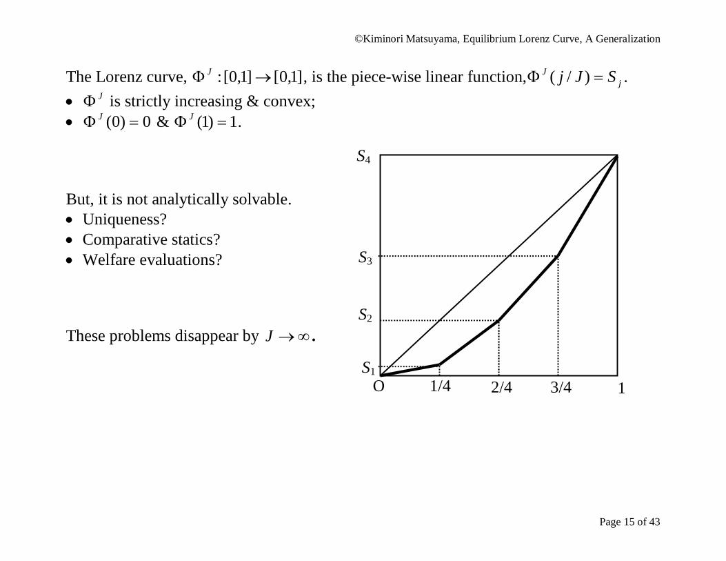
The Lorenz curve, ]1,0[]1,0[: J , is the piece-wise linear function, jJ SJj )/( .
J is strictly increasing & convex; 0)0( J & 1)1( J . But, it is not analytically solvable. Uniqueness? Comparative statics? Welfare evaluations? These problems disappear by J .
2/4 O
S4
1 3/4 1/4
S3
S2
S1
©Kiminori Matsuyama, Equilibrium Lorenz Curve, A Generalization
Page 16 of 43
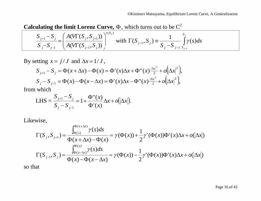
Calculating the limit Lorenz Curve, , which turns out to be C2
)(
1
1
1
1
)),(()),(( jS
jj
jj
jj
jj
SSVASSVA
SSSS
with
j
j
S
Sjjjj dss
SSSS
1
)(1),(1
1
By setting Jjx / and Jx /1 ,
221
2
)(")(')()( xoxxxxxxSS xjj
,
221
2
)(")(')()( xoxxxxxxSS xjj ,
from which
LHS = xoxxx
SSSS
jj
jj
)(')("1
1
1 .
Likewise,
)()('))(('21))((
)()(
)(),(
)(
)(1 xoxxxx
xxx
dssSS
xx
xjj
)()('))(('21))((
)()(
)(),(
)(
)(1 xoxxxx
xxx
dssSS
x
xxjj
so that
©Kiminori Matsuyama, Equilibrium Lorenz Curve, A Generalization
Page 17 of 43
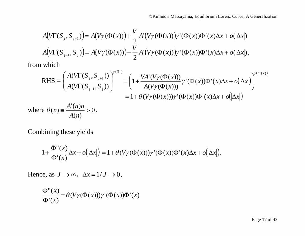
)()('))(('))(('2
))((),( 1 xoxxxxVAVxVASSVA jj
)()('))(('))(('2
))((),( 1 xoxxxxVAVxVASSVA jj ,
from which
RHS = )(
1
1
)),(()),(( jS
jj
jj
SSVASSVA
)(
)('))((')))((()))((('1
x
xoxxxxVAxVVA
xoxxxxV )('))((')))(((1
where 0)()(')(
nAnnAn .
Combining these yields
xoxxx
)(')("1 xoxxxxV )('))((')))(((1 .
Hence, as J , 0/1 Jx ,
)(')("
xx
)('))((')))((( xxxV
©Kiminori Matsuyama, Equilibrium Lorenz Curve, A Generalization
Page 18 of 43
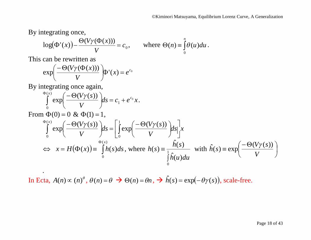
By integrating once,
)('log x 0)))((( c
VxV
, where
n
duun0
)()( .
This can be rewritten as 0)(')))(((exp cex
VxV
By integrating once again,
xecdsV
sV cx
01
)(
0
))((exp
.
From 0)0( & 1)1( ,
xdsV
sVdsV
sVx
1
0
)(
0
))((exp))((exp
)(
0
)()(x
dsshxHx , where
1
0)(ˆ)(ˆ)(duuh
shsh with
V
sVsh ))((exp)(ˆ
. In Ecta, )()( nnA , )(n nn )( , )(exp)(ˆ ssh , scale-free.
©Kiminori Matsuyama, Equilibrium Lorenz Curve, A Generalization
Page 19 of 43
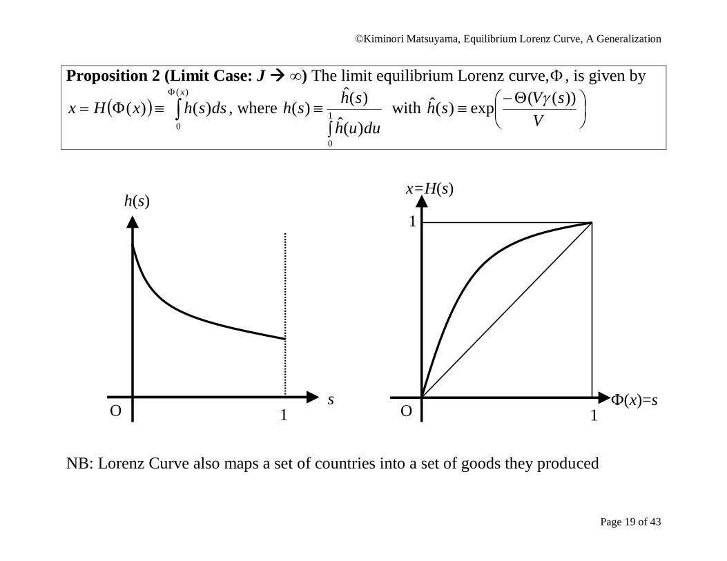
Proposition 2 (Limit Case: J ∞) The limit equilibrium Lorenz curve, , is given by
)(
0
)()(x
dsshxHx , where
1
0)(ˆ)(ˆ)(duuh
shsh with
V
sVsh ))((exp)(ˆ
NB: Lorenz Curve also maps a set of countries into a set of goods they produced
O 1
Ф(x)=s
1
x=H(s)
O 1
s
h(s)
©Kiminori Matsuyama, Equilibrium Lorenz Curve, A Generalization
Page 20 of 43
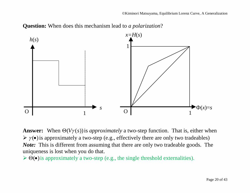
Question: When does this mechanism lead to a polarization? Answer: When ))(( sV is approximately a two-step function. That is, either when )( is approximately a two-step (e.g., effectively there are only two tradeables) Note: This is different from assuming that there are only two tradeable goods. The uniqueness is lost when you do that. )( is approximately a two-step (e.g., the single threshold externalities).
O 1
s
h(s)
O 1
Ф(x)=s
1
x=H(s)
©Kiminori Matsuyama, Equilibrium Lorenz Curve, A Generalization
Page 21 of 43
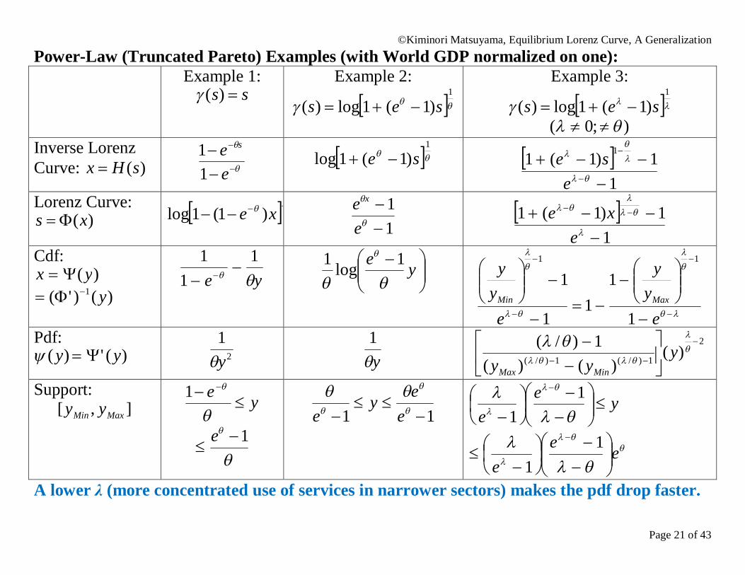
Power-Law (Truncated Pareto) Examples (with World GDP normalized on one): Example 1:
ss )( Example 2:
1
)1(1log)( ses
Example 3:
1
)1(1log)( ses );0(
Inverse Lorenz Curve: )(sHx
ee s
11
1
)1(1log se 1
1)1(1 1
ese
Lorenz Curve: )(xs )1(1log xe
11
ee x
1
1)1(1
exe
Cdf: )(yx
)()'( 1 y ye
11
1
ye
1log1
ey
y
ey
y
MaxMin
1
11
1
111
Pdf: )( y )(' y 2
1y
y1 2
1)/(1)/( )()()(
1)/(
yyy MinMax
Support: ],[ MaxMin yy ye
1
1
e
11
e
eye
yee
11
ee
e
11
A lower λ (more concentrated use of services in narrower sectors) makes the pdf drop faster.
©Kiminori Matsuyama, Equilibrium Lorenz Curve, A Generalization
Page 22 of 43
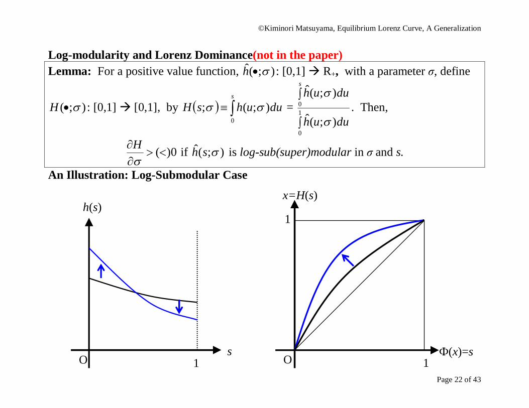
Log-modularity and Lorenz Dominance(not in the paper) Lemma: For a positive value function, );(ˆ h : [0,1] R+, with a parameter σ, define
);( H : [0,1] [0,1], by s
duuhsH0
);(; =
1
0
0
);(ˆ
);(ˆ
duuh
duuhs
. Then,
0)(H if );(ˆ sh is log-sub(super)modular in σ and s.
An Illustration: Log-Submodular Case
O 1
s
h(s)
O 1
Ф(x)=s
1
x=H(s)
©Kiminori Matsuyama, Equilibrium Lorenz Curve, A Generalization
Page 23 of 43
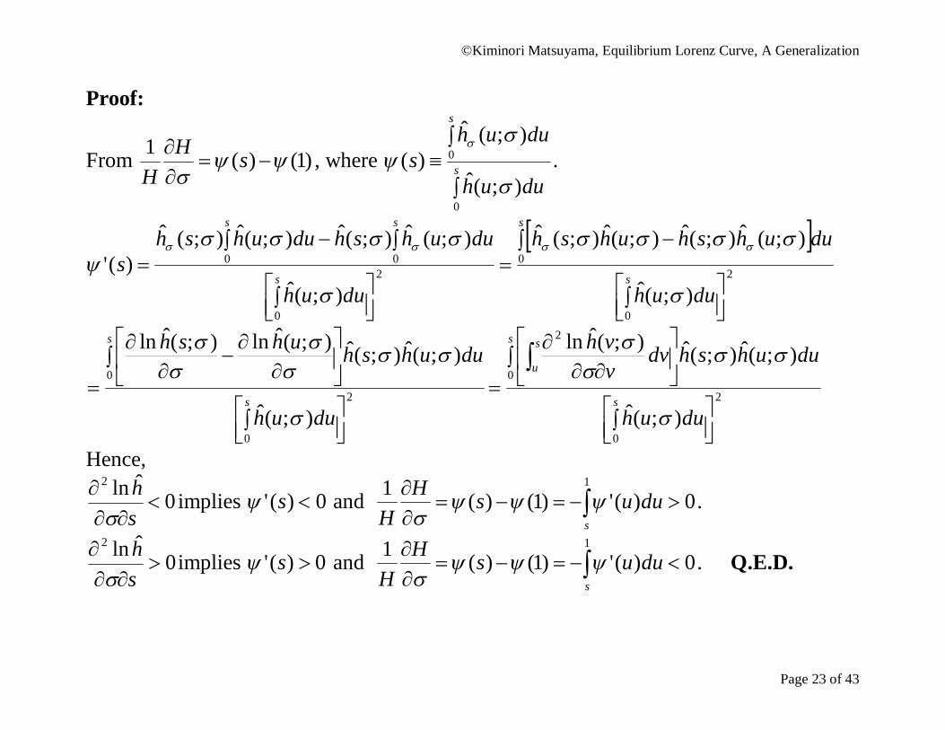
Proof:
From )1()(1
sH
H, where
s
s
duuh
duuhs
0
0
);(ˆ
);(ˆ)(
.
2
0
02
0
0 0
);(ˆ
);(ˆ);(ˆ);(ˆ);(ˆ
);(ˆ
);(ˆ);(ˆ);(ˆ);(ˆ)('
s
s
s
s s
duuh
duuhshuhsh
duuh
duuhshduuhshs
2
0
0
);(ˆ
);(ˆ);(ˆ);(ˆln);(ˆln
s
s
duuh
duuhshuhsh
2
0
0
2
);(ˆ
);(ˆ);(ˆ);(ˆln
s
s s
u
duuh
duuhshdvvvh
Hence,
0ˆln2
sh
implies 0)(' s and 0)(')1()(1 1
s
duusHH
.
0ˆln2
sh
implies 0)(' s and 0)(')1()(1 1
s
duusHH
. Q.E.D.
©Kiminori Matsuyama, Equilibrium Lorenz Curve, A Generalization
Page 24 of 43
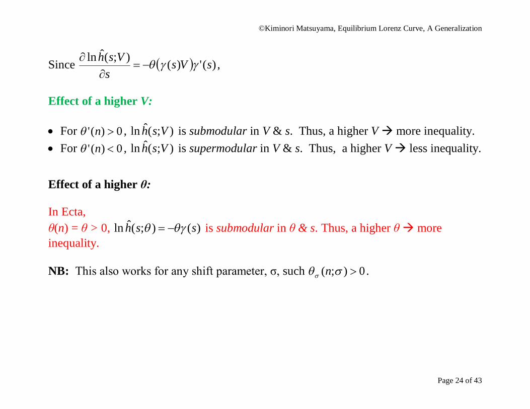
Since )(')();(ˆln sVss
Vsh
,
Effect of a higher V: For 0)(' n , );(ˆln Vsh is submodular in V & s. Thus, a higher V more inequality. For 0)(' n , );(ˆln Vsh is supermodular in V & s. Thus, a higher V less inequality.
Effect of a higher θ: In Ecta, θ(n) = θ > 0, )();(ˆln ssh is submodular in θ & s. Thus, a higher θ more inequality. NB: This also works for any shift parameter, σ, such 0);( n .
©Kiminori Matsuyama, Equilibrium Lorenz Curve, A Generalization
Page 25 of 43
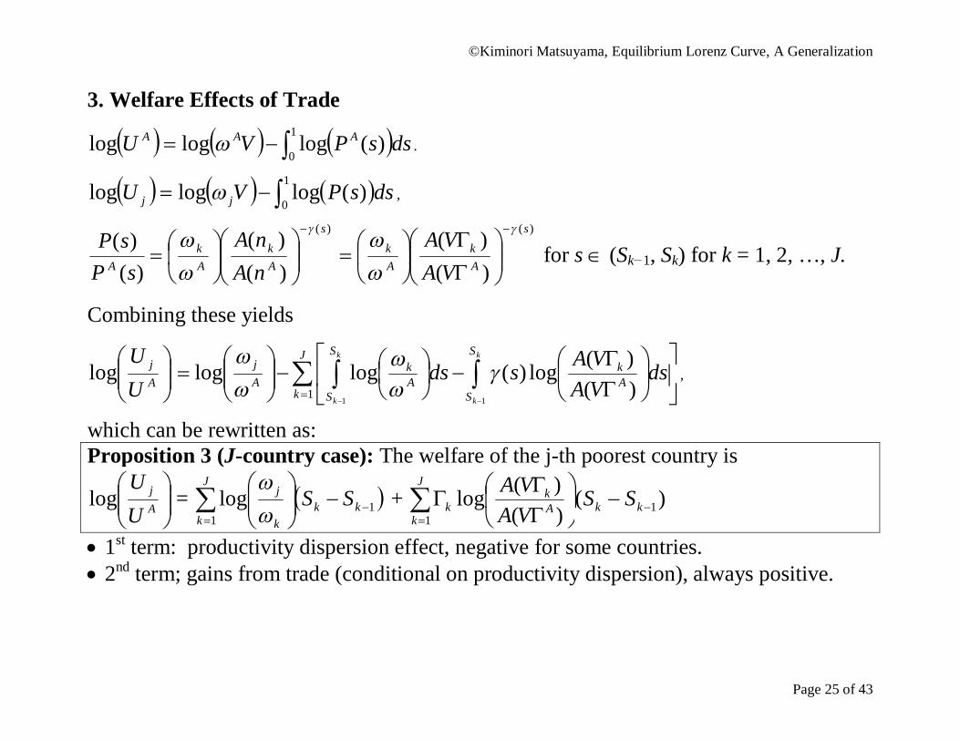
3. Welfare Effects of Trade
1
0)(logloglog dssPVU AAA .
1
0)(logloglog dssPVU jj ,
)()(
)()(
)()(
)()(
s
Ak
Ak
s
Ak
Ak
A VAVA
nAnA
sPsP
for s (Sk−1, Sk) for k = 1, 2, …, J.
Combining these yields
Aj
UU
log
J
k
S
SAk
S
SAk
Aj
k
k
k
k
dsVAVAsds
1 11)()(log)(loglog
,
which can be rewritten as: Proposition 3 (J-country case): The welfare of the j-th poorest country is
Aj
UU
log =
J
kkk
k
j SS1
1log
+
J
kkkA
kk SS
VAVA
11)(
)()(log
1st term: productivity dispersion effect, negative for some countries. 2nd term; gains from trade (conditional on productivity dispersion), always positive.
©Kiminori Matsuyama, Equilibrium Lorenz Curve, A Generalization
Page 26 of 43
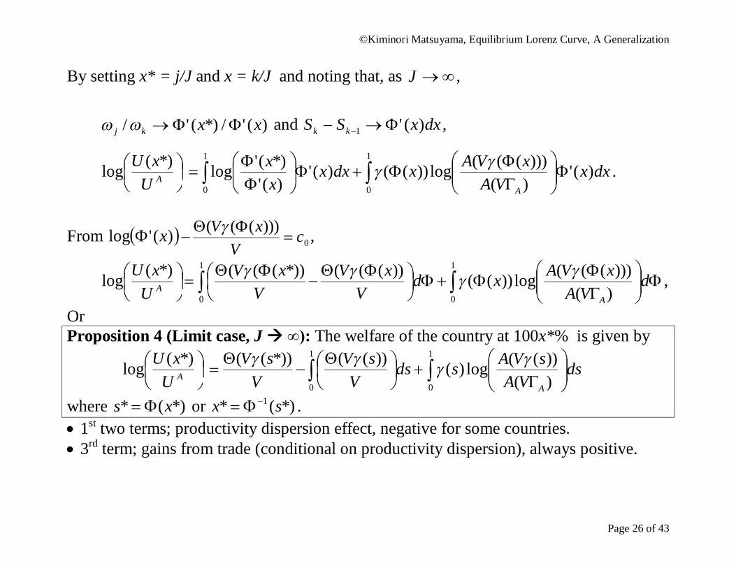
By setting x* = j/J and x = k/J and noting that, as J ,
)('/*)('/ xxkj and dxxSS kk )('1 ,
AUxU *)(log
1
0
1
0
)(')()))(((log))(()('
)('*)('log dxx
VAxVAxdxx
xx
A
.
From )('log x 0)))((( c
VxV
,
AUxU *)(log
1
0
))(((*))((( dV
xVV
xV
1
0 )()))(((log))(( d
VAxVAx
A
,
Or Proposition 4 (Limit case, J ∞): The welfare of the country at 100x*% is given by
AUxU *)(log
1
0
))((*))(( dsV
sVV
sV
1
0 )())((log)( ds
VAsVAsA
where *)(* xs or *)(* 1 sx . 1st two terms; productivity dispersion effect, negative for some countries. 3rd term; gains from trade (conditional on productivity dispersion), always positive.
©Kiminori Matsuyama, Equilibrium Lorenz Curve, A Generalization
Page 27 of 43
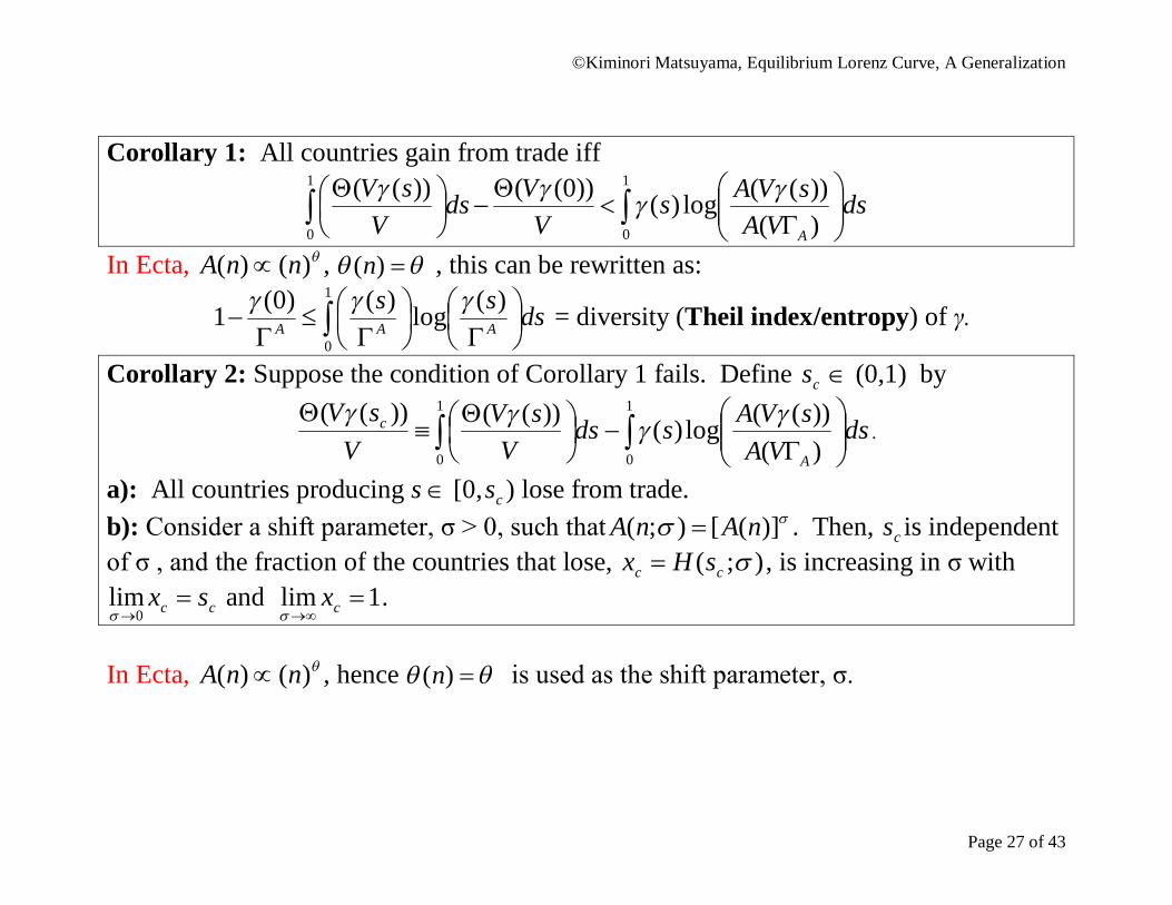
Corollary 1: All countries gain from trade iff
V
VdsV
sV ))0(())((1
0
1
0 )())((log)( ds
VAsVAsA
In Ecta, )()( nnA , )(n , this can be rewritten as:
1
0
)(log)()0(1 dsssAAA
= diversity (Theil index/entropy) of γ.
Corollary 2: Suppose the condition of Corollary 1 fails. Define cs (0,1) by
VsV c ))((
1
0
))(( dsV
sV
1
0 )())((log)( ds
VAsVAsA
.
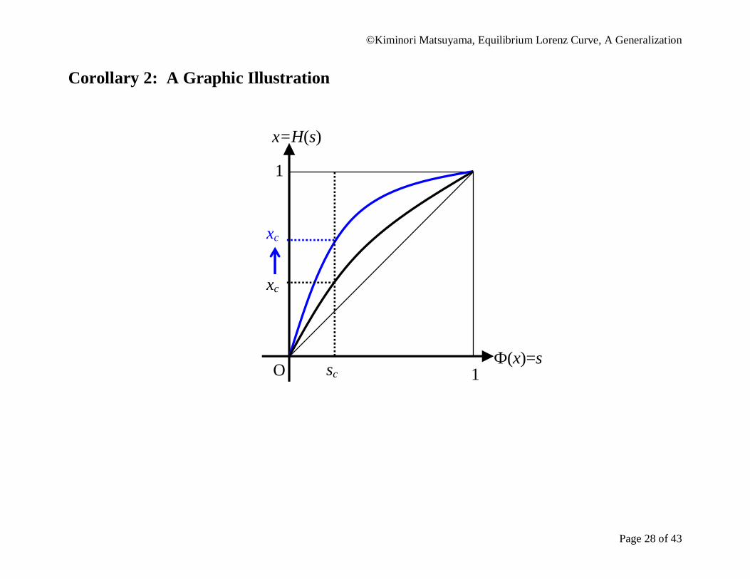
a): All countries producing s [0, cs ) lose from trade. b): Consider a shift parameter, σ > 0, such that )]([);( nAnA . Then, cs is independent of σ , and the fraction of the countries that lose, );( cc sHx , is increasing in σ with
cc sx 0
lim
and 1lim cx
.
In Ecta, )()( nnA , hence )(n is used as the shift parameter, σ.
©Kiminori Matsuyama, Equilibrium Lorenz Curve, A Generalization
Page 28 of 43
Corollary 2: A Graphic Illustration
sc O 1
Ф(x)=s
1
x=H(s)
xc
xc
©Kiminori Matsuyama, Equilibrium Lorenz Curve, A Generalization
Page 29 of 43
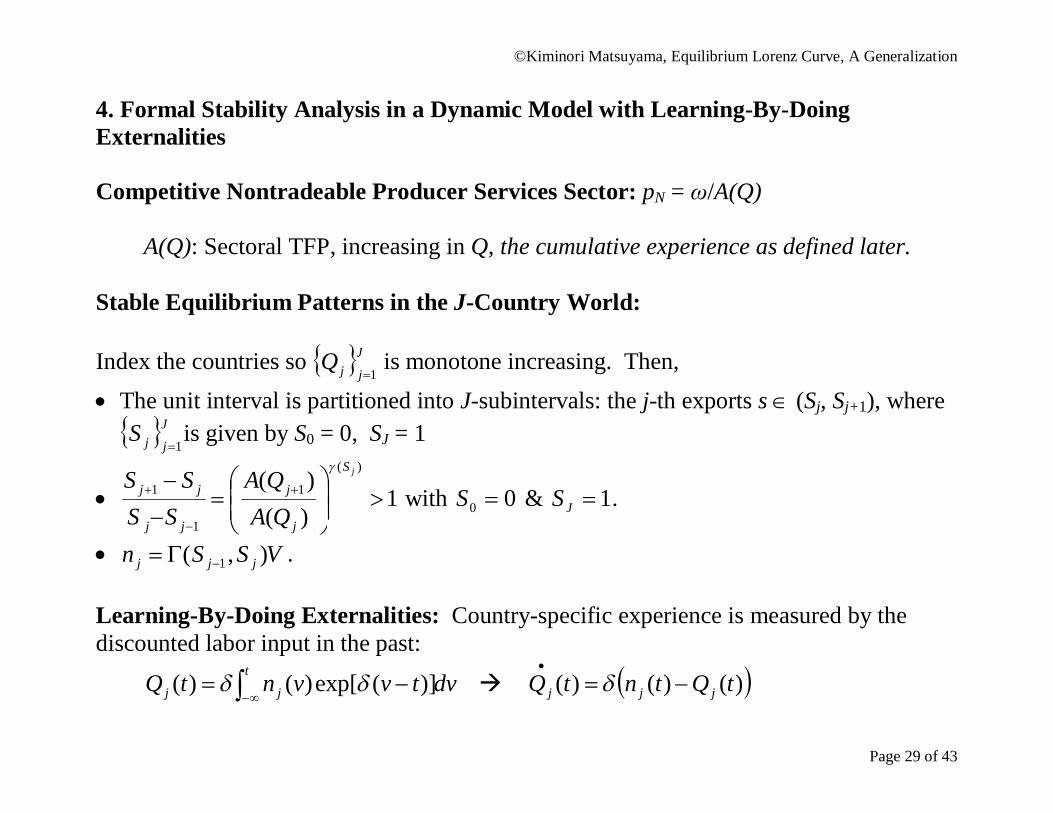
4. Formal Stability Analysis in a Dynamic Model with Learning-By-Doing Externalities Competitive Nontradeable Producer Services Sector: pN = ω/A(Q)
A(Q): Sectoral TFP, increasing in Q, the cumulative experience as defined later.
Stable Equilibrium Patterns in the J-Country World: Index the countries so J
jjQ1 is monotone increasing. Then,
The unit interval is partitioned into J-subintervals: the j-th exports s (Sj, Sj+1), where J
jjS1is given by S0 = 0, SJ = 1
1)()(
)(
1
1
1
jS
j
j
jj
jj
QAQA
SSSS
with 00 S & 1JS .
VSSn jjj ),( 1 . Learning-By-Doing Externalities: Country-specific experience is measured by the discounted labor input in the past:
dvtvvntQt
jj )](exp[)()( )()()( tQtntQ jjj
©Kiminori Matsuyama, Equilibrium Lorenz Curve, A Generalization
Page 30 of 43
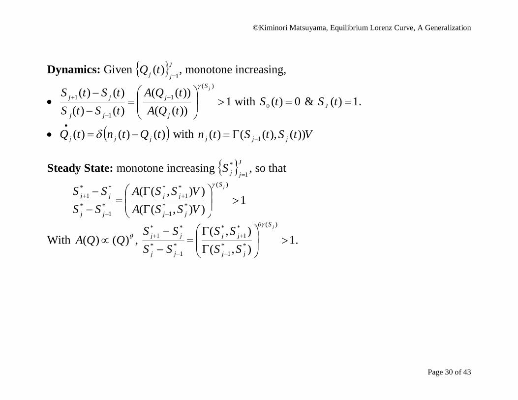
Dynamics: Given J
jj tQ1
)(
, monotone increasing,
1))(())((
)()()()(
)(
1
1
1
jS
j
j
jj
jj
tQAtQA
tStStStS
with 0)(0 tS & 1)( tS J .
)()()( tQtntQ jjj
with VtStStn jjj ))(),(()( 1 Steady State: monotone increasing J
jjS1
*
, so that
1)),(()),((
)(
**1
*1
*
*1
*
**1
jS
jj
jj
jj
jj
VSSAVSSA
SSSS
With )()( QQA , 1),(),(
)(
**1
*1
*
*1
*
**1
jS
jj
jj
jj
jj
SSSS
SSSS
.
©Kiminori Matsuyama, Equilibrium Lorenz Curve, A Generalization
Page 31 of 43
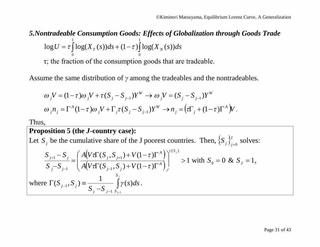
5.Nontradeable Consumption Goods: Effects of Globalization through Goods Trade
1
0
1
0
))(log()1())(log(log dssXdssXU NT
τ; the fraction of the consumption goods that are tradeable. Assume the same distribution of γ among the tradeables and the nontradeables.
W
jjjj YSSVV )()1( 1 W
jjj YSSV )( 1
W
jjjjA
jj YSSVn )()1( 1 Vn Ajj )1( .
Thus, Proposition 5 (the J-country case): Let jS be the cumulative share of the J poorest countries. Then, J
jjS0 solves:
1
)1(),()1(),(
)(
1
1
1
1
jS
Ajj
Ajj
jj
jj
VSSVAVSSVA
SSSS
with 00 S & 1JS ,
where
j
j
S
Sjjjj dss
SSSS
1
)(1),(1
1 .
©Kiminori Matsuyama, Equilibrium Lorenz Curve, A Generalization
Page 32 of 43
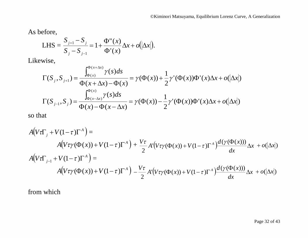
As before,
LHS = xoxxx
SSSS
jj
jj
)(')("1
1
1 .
Likewise,
)()('))(('21))((
)()(
)(),(
)(
)(1 xoxxxx
xxx
dssSS
xx
xjj
)()('))(('21))((
)()(
)(),(
)(
)(1 xoxxxx
xxx
dssSS
x
xxjj
so that A
j VVA )1( =
AVxVA )1())(( + xdx
xdVxVAV A
)))((()1())(('
2
)( xo
Aj VVA )1(1 =
AVxVA )1())(( xdx
xdVxVAV A
)))((()1())(('
2
)( xo
from which
©Kiminori Matsuyama, Equilibrium Lorenz Curve, A Generalization
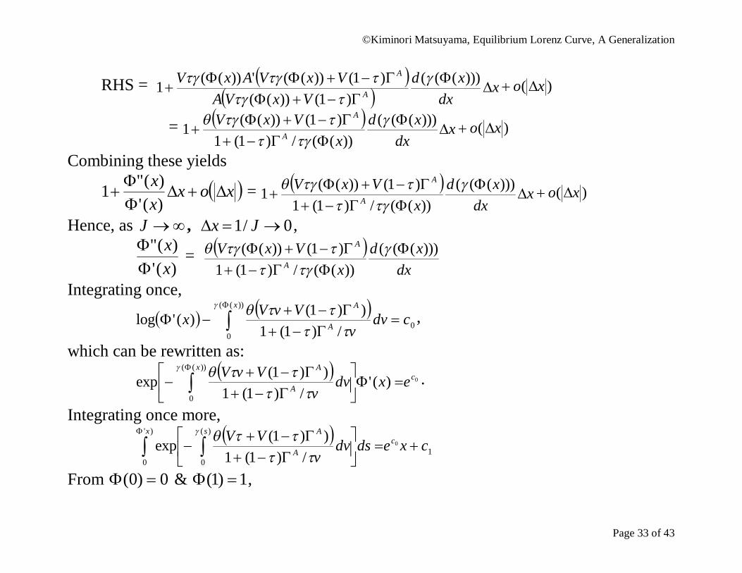
Page 33 of 43
RHS = x
dxxd
VxVAVxVAxV
A
A
)))(((
)1())(()1())(('))((1
)( xo
= xdx
xdx
VxVA
A
)))(((
))((/)1(1)1())((1
)( xo
Combining these yields
xoxxx
)(')("1 = x
dxxd
xVxV
A
A
)))(((
))((/)1(1)1())((1
)( xo
Hence, as J , 0/1 Jx ,
)(')("
xx
=
dxxd
xVxV
A
A )))((())((/)1(1
)1())((
Integrating once,
0
))((
0 /)1(1))1()('log cdv
vVvVx
x
A
A
,
which can be rewritten as:
0)('/)1(1
))1(exp))((
0
cx
A
A
exdvv
VvV
.
Integrating once more,
1
)'
0
)(
0
0
/)1(1))1(exp cxedsdv
vVV c
x s
A
A
From 0)0( & 1)1( ,
©Kiminori Matsuyama, Equilibrium Lorenz Curve, A Generalization
Page 34 of 43
xdsdvv
VvVdsdvv
VvV s
A
Ax s
A
A
1
0
)(
0
)'
0
)(
0 /)1(1))1(exp
/)1(1))1(exp
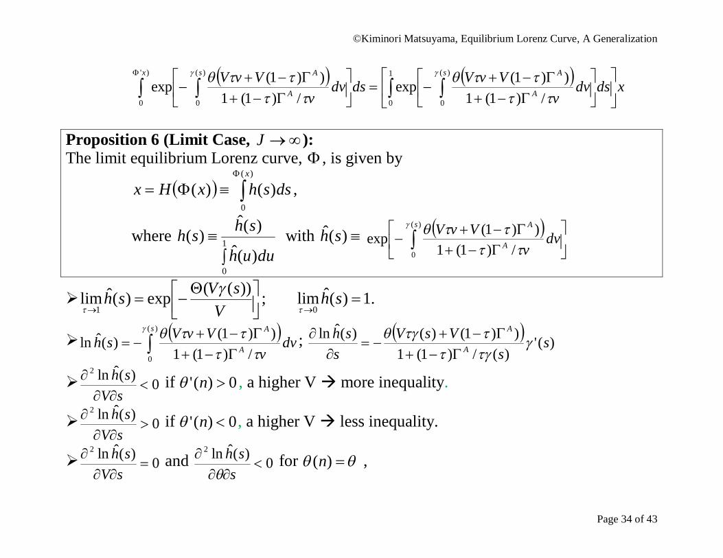
Proposition 6 (Limit Case, J ): The limit equilibrium Lorenz curve, , is given by
)(
0
)()(x
dsshxHx ,
where
1
0)(ˆ)(ˆ)(duuh
shsh with )(ˆ sh
)(
0 /)1(1))1(exp
s
A
A
dvv
VvV
VsVsh ))((exp)(ˆlim
1
; 1)(ˆlim0
sh
.
)(
0 /)1(1))1()(ˆln
s
A
A
dvv
VvVsh
; )('
)(/)1(1))1()()(ˆln s
sVsV
ssh
A
A
0)(ˆln2
sV
sh if 0)(' n , a higher V more inequality.
0)(ˆln2
sV
sh if 0)(' n , a higher V less inequality.
0)(ˆln2
sV
sh and 0)(ˆln2
s
sh
for )(n ,
©Kiminori Matsuyama, Equilibrium Lorenz Curve, A Generalization
Page 35 of 43
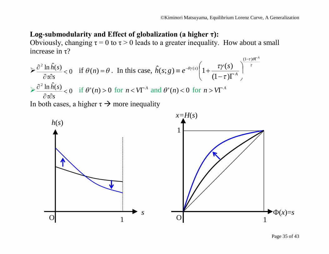
Log-submodularity and Effect of globalization (a higher τ): Obviously, changing τ = 0 to τ > 0 leads to a greater inequality. How about a small increase in τ?
0)(ˆln2
s
sh
if )(n . In this case,
A
As segsh
)1(
)(
)1()(1);(ˆ
0)(ˆln2
s
sh
if 0)(' n for AVn and 0)(' n for AVn
In both cases, a higher τ more inequality
O 1
s
h(s)
O 1
Ф(x)=s
1
x=H(s)
©Kiminori Matsuyama, Equilibrium Lorenz Curve, A Generalization
Page 36 of 43
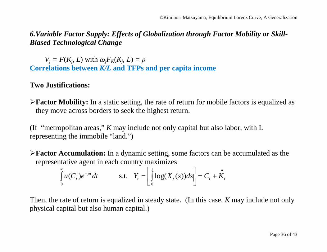
6.Variable Factor Supply: Effects of Globalization through Factor Mobility or Skill-Biased Technological Change
Vj = F(Kj, L) with ωjFK(Kj, L) = ρ Correlations between K/L and TFPs and per capita income Two Justifications: Factor Mobility: In a static setting, the rate of return for mobile factors is equalized as
they move across borders to seek the highest return. (If “metropolitan areas,” K may include not only capital but also labor, with L representing the immobile “land.”) Factor Accumulation: In a dynamic setting, some factors can be accumulated as the
representative agent in each country maximizes
0
)( dteCu tt
s.t.
tttt KCdssXY1
0
))(log(
Then, the rate of return is equalized in steady state. (In this case, K may include not only physical capital but also human capital.)
©Kiminori Matsuyama, Equilibrium Lorenz Curve, A Generalization
Page 37 of 43
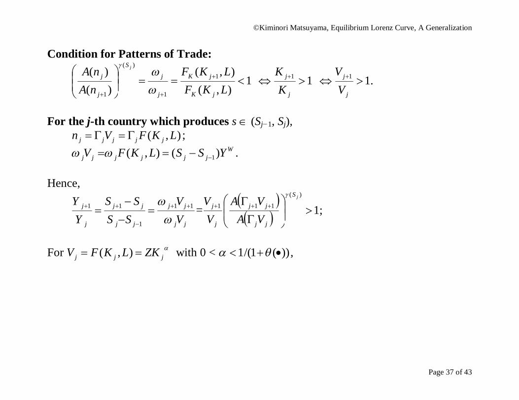
Condition for Patterns of Trade:
1),(),(
)()( 1
1
)(
1
LKFLKF
nAnA
jK
jK
j
j
S
j
jj
11
j
j
KK
11
j
j
VV
.
For the j-th country which produces s (Sj−1, Sj), ),( LKFVn jjjjj ;
Wjjjjjj YSSLKFV )(),( 1 .
Hence,
jj
jj
jj
jj
j
j
VV
SSSS
YY
11
1
11
=
1
)(
111
jS
jj
jj
j
j
VAVA
VV
;
For
jjj ZKLKFV ),( with 0 < ))(1/(1 ,
©Kiminori Matsuyama, Equilibrium Lorenz Curve, A Generalization
Page 38 of 43
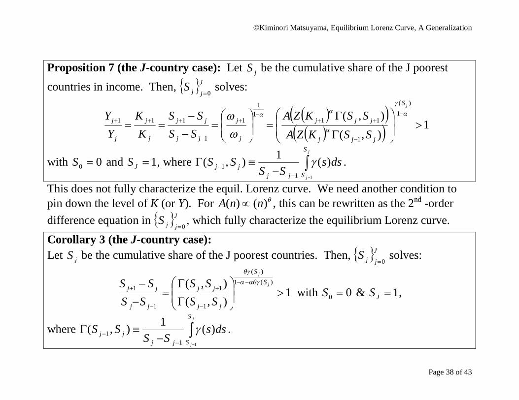
Proposition 7 (the J-country case): Let jS be the cumulative share of the J poorest countries in income. Then, J
jjS0 solves:
11
1
1
111
j
j
jj
jj
j
j
j
j
SSSS
KK
YY
1),(),( 1
)(
1
11
jS
jjj
jjj
SSKZASSKZA
with 00 S and 1JS , where
j
j
S
Sjjjj dss
SSSS
1
)(1),(1
1 .
This does not fully characterize the equil. Lorenz curve. We need another condition to pin down the level of K (or Y). For )()( nnA , this can be rewritten as the 2nd -order difference equation in J
jjS0, which fully characterize the equilibrium Lorenz curve.
Corollary 3 (the J-country case): Let jS be the cumulative share of the J poorest countries. Then, J
jjS0 solves:
1),(),( )(1
)(
1
1
1
1
j
j
SS
jj
jj
jj
jj
SSSS
SSSS
with 00 S & 1JS ,
where
j
j
S
Sjjjj dss
SSSS
1
)(1),(1
1 .
©Kiminori Matsuyama, Equilibrium Lorenz Curve, A Generalization
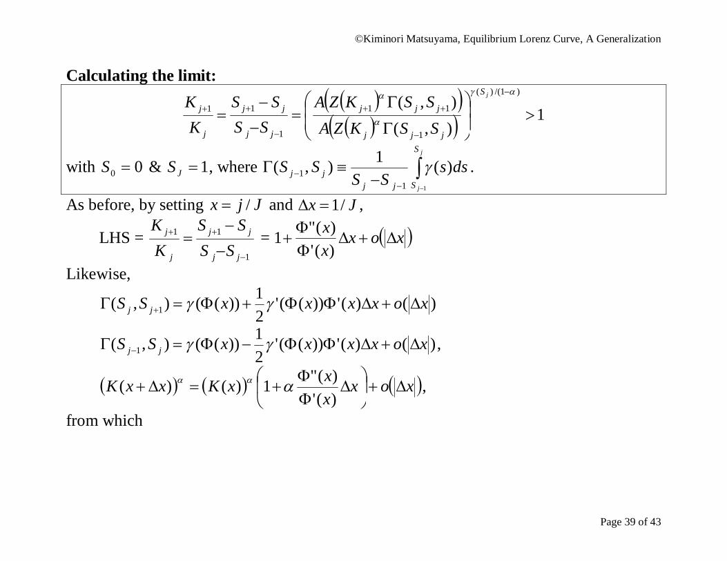
Page 39 of 43
Calculating the limit:
j
j
KK 1
1),(),(
)1/()(
1
11
1
1
jS
jjj
jjj
jj
jj
SSKZASSKZA
SSSS
with 00 S & 1JS , where
j
j
S
Sjjjj dss
SSSS
1
)(1),(1
1 .
As before, by setting Jjx / and Jx /1 ,
LHS = 1
11
jj
jj
j
j
SSSS
KK
= xoxxx
)(')("1
Likewise,
)()('))(('21))((),( 1 xoxxxxSS jj
)()('))(('21))((),( 1 xoxxxxSS jj ,
)()( xKxxK xoxxx
)(')("1 ,
from which
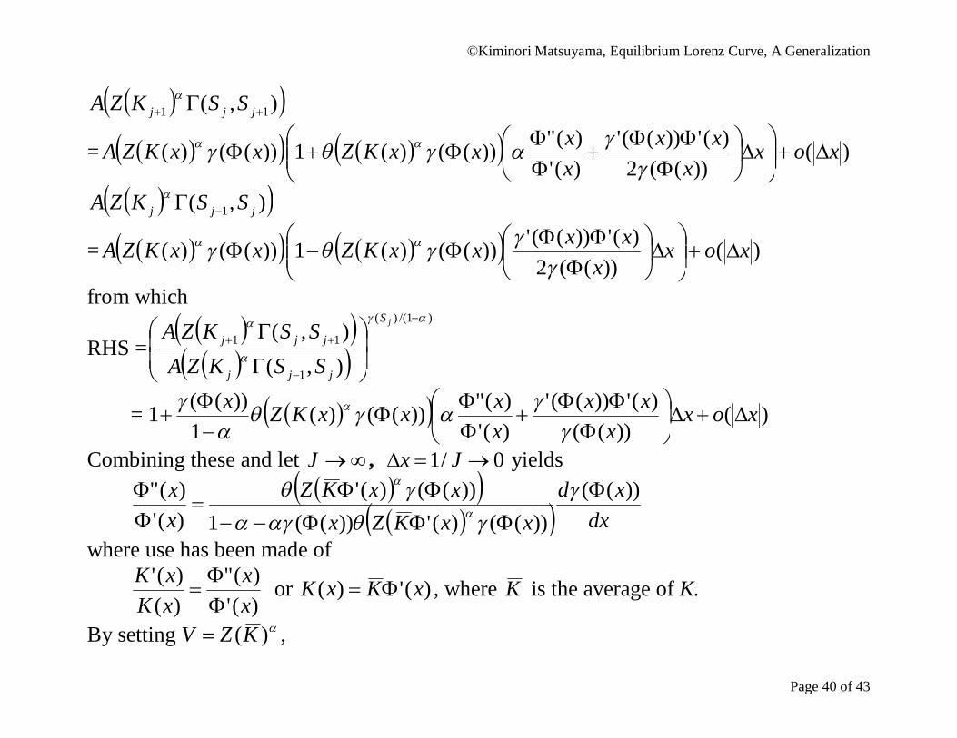
©Kiminori Matsuyama, Equilibrium Lorenz Curve, A Generalization
Page 40 of 43
),( 11 jjj SSKZA
= ))(()( xxKZA )())((2
)('))((')(')("))(()(1 xox
xxx
xxxxKZ
),( 1 jjj SSKZA
= ))(()( xxKZA )())((2
)('))(('))(()(1 xoxx
xxxxKZ
from which
RHS =
)1/()(
1
11
),(),(
jS
jjj
jjj
SSKZASSKZA
= )())((
)('))((')(')("))(()(
1))((1 xox
xxx
xxxxKZx
Combining these and let J , 0/1 Jx yields
dxxd
xxKZxxxKZ
xx ))((
))(()('))((1))(()('
)(')("
where use has been made of
)(')("
)()('
xx
xKxK
or )(')( xKxK , where K is the average of K.
By setting )(KZV ,
©Kiminori Matsuyama, Equilibrium Lorenz Curve, A Generalization
Page 41 of 43
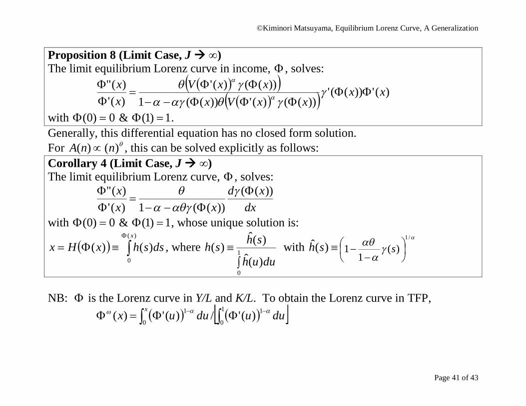
Proposition 8 (Limit Case, J ∞) The limit equilibrium Lorenz curve in income, , solves:
)('))(('
))(()('))((1))(()('
)(')(" xx
xxVxxxV
xx
with 0)0( & 1)1( . Generally, this differential equation has no closed form solution. For )()( nnA , this can be solved explicitly as follows: Corollary 4 (Limit Case, J ∞) The limit equilibrium Lorenz curve, , solves:
dxxd
xxx ))((
))((1)(')("
with 0)0( & 1)1( , whose unique solution is:
)(
0
)()(x
dsshxHx , where
1
0)(ˆ)(ˆ)(duuh
shsh with )(ˆ sh
/1
)(1
1
s
NB: is the Lorenz curve in Y/L and K/L. To obtain the Lorenz curve in TFP,
1
0
1
0
1 )('/)(')( duuduuxx
©Kiminori Matsuyama, Equilibrium Lorenz Curve, A Generalization
Page 42 of 43
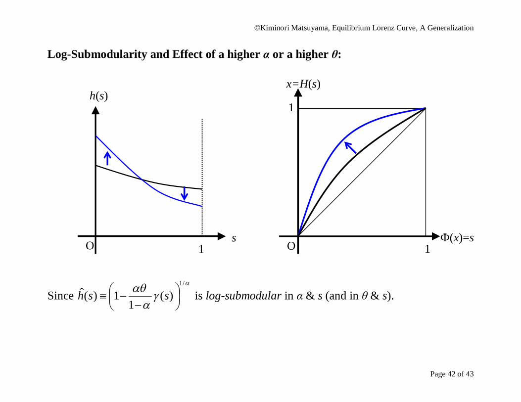
Log-Submodularity and Effect of a higher α or a higher θ:
Since
/1
)(1
1)(ˆ
ssh is log-submodular in α & s (and in θ & s).
O 1
s
h(s)
O 1
Ф(x)=s
1
x=H(s)
©Kiminori Matsuyama, Equilibrium Lorenz Curve, A Generalization
Page 43 of 43
7. Some Concluding Remarks: Symmetry-breaking in general Symmetry-breaking due to two-way causality; Even without ex-ante heterogeneity,
cross-country dispersion and correlations in per capita income, TFPs, and K/L ratios emerge as stable equilibrium patterns due to interaction through trade.
Some countries become richer (poorer) than others because they trade with poorer (richer) countries. They are not independent observations.
This type of analysis does not say that ex-ante heterogeneity is unimportant. Instead, it says that even small ex-ante heterogeneity could be magnified to create huge ex-post heterogeneity, a possible explanation of Great Divergence and Growth Miracle
This paper in particular This paper demonstrates that this type of analysis does not have to be intractable nor
lacking in prediction. Equilibrium distribution is unique, analytically solvable, varying with parameters in intuitive ways.
With a finite countries and a continuum of sectors, this model is more compatible with existing quantitative models of trade (Eaton-Kortum, Alvarez-Lucas, etc.)
A model with many countries can be more tractable than a model with a few countries.