equity market volatility and expected risk premium in this paper we reexamine the intertemporal...
TRANSCRIPT

Research Division Federal Reserve Bank of St. Louis Working Paper Series
Equity Market Volatility and Expected Risk Premium
Long Chen Hui Guo
and Lu Zhang
Working Paper 2006-007A http://research.stlouisfed.org/wp/2006/2006-007.pdf
January 2006
FEDERAL RESERVE BANK OF ST. LOUIS Research Division
P.O. Box 442 St. Louis, MO 63166
______________________________________________________________________________________
The views expressed are those of the individual authors and do not necessarily reflect official positions of the Federal Reserve Bank of St. Louis, the Federal Reserve System, or the Board of Governors.
Federal Reserve Bank of St. Louis Working Papers are preliminary materials circulated to stimulate discussion and critical comment. References in publications to Federal Reserve Bank of St. Louis Working Papers (other than an acknowledgment that the writer has had access to unpublished material) should be cleared with the author or authors.

Equity Market Volatility and Expected Risk Premium
Long Chena, Hui Guob, and Lu Zhangc
January 26, 2006
Abstract
This paper revisits the time-series relation between the conditional risk premium and variance of the equity market portfolio. The main innovation is that we construct a measure of the ex ante equity market risk premium using corporate bond yield spread data. This measure is forward-looking and does not rely critically on either realized equity returns or instrumental variables. We find strong support for a positive risk-return tradeoff, and this result is not sensitive to a number of robustness checks, including alternative proxies of the conditional stock variance and controls for hedging demands. JEL Classification: G12, E44 Key Words: Expected return, equity market volatility, systematic risk, yield spreads
a Department of Finance, The Eli Broad College of Business, Michigan State University, East Lansing, MI 48824, E-mail: [email protected]. b Research Division, The Federal Reserve Bank of St. Louis, P.O. Box 442, St. Louis, MO 63166-0442, E-mail: [email protected]. c William E. Simon Graduate School of Business Administration, University of Rochester, Rochester, NY 14627, E-mail: [email protected]. We thank Jason Higbee for excellent research assistant. The views expressed in this paper are those of the authors and do not necessarily reflect the official positions of the Federal Reserve Bank of St. Louis or the Federal Reserve System.

1
I. Introduction
Standard asset pricing theory, e.g., the capital asset pricing model (CAPM),
predicts that investors demand an ex ante risk premium for bearing the systematic risk
that they cannot diversify away. The market portfolio in the equity market is the most
diversified portfolio; as such, its conditional variance represents one of the most
commonly used measures of market systematic risk. A positive relation between the
expected return and variance of the market portfolio is intuitively appealing and Ghysels,
Santa-Clara, and Valkanov (2005) argue that it is the “first fundamental law of finance.”
The empirical evidence on this relation, however, has been mixed. Some authors,
including Pindyck (1984), French, Schwert, and Stambaugh (1987), and Ghysels, Santa-
Clara, and Valkanov (2005), find that, consistent with CAPM, the conditional excess
stock market return is positively related to the conditional stock market variance. Many
others, including Campbell (1987), Glosten, Jagannathan, and Runkle (1993), Whitelaw
(1994), Lettau and Ludvigson (2003), and Brandt and Kang (2004), document a
significantly negative risk-return tradeoff in the data.
One important reason for the conflicting results could be that the expected return
is unobservable. The early studies had to use either realized stock returns or instrumental
variables as proxies for it. Such practice, albeit usually out of necessity, has its
limitations. For example, as pointed out by Elton (1999), realized returns are a poor
measure of expected returns.1 Similarly, Campbell (1987), among others, finds that the
results are sensitive to the choice of instrumental variables.
1 While discussing the limitation of using realized returns as the proxy for expected returns, Elton (1999) makes the following statement in his American Finance Association presidential address:"[D]eveloping better measures of expected return and alternative ways of testing asset pricing theories that do not require using realized returns have a much higher payoff than any additional development of statistical tests that continue to rely on realized returns as a proxy for expected returns” (p. 1200).

2
In this paper we reexamine the intertemporal risk-return tradeoff by using a direct
measure of the expected return, as developed by Campello, Chen, and Zhang (2005, CCZ
hereafter). Such a measure makes use of the intuition that, because debt and equity are
financial claims written on the same corporation productions, they must share the same
systematic risk that affects firm fundamentals. The yield spread—the difference between
the corporate bond yield and the Treasury bond yield—incorporates both the fair
compensation for default risk and the ex ante risk premium. It is well known in the
default risk literature that the fair compensation for default risk is only a relatively small
portion of the yield spread (e.g., Jones, Mason, and Rosenfeld (1984) and Huang and
Huang (2003)). Therefore, even though the fair default risk compensation needs to be
estimated using past information, the yield spread adjusted by this estimate retains largely
the forward-looking property of the ex ante risk premium. CCZ provide an analytical
formula that links the ex ante equity risk premium to the yield spread after adjusting for
the estimated fair compensation for default risk and for the tax effects. We follow CCZ to
construct the ex ante equity risk premium. This risk premium not only is forward looking,
but also does not rely critically on the choice of instrumental variables.
We then turn to estimate the conditional volatility of the market portfolio.
Following Campbell (1987), French, Schwert, and Stambaugh (1987), and Whitelaw
(1994), we estimate conditional variance using the instrumental variables approach.2 In
particular, as in Merton (1980) and Andersen, Bollerslev, Diebold, and Labys (2003), we
construct monthly realized stock market variance (RV) using daily data and use lagged
RV as a proxy for the conditional variance. To be robust, we also use more elaborate
2 One important advantage of the instrumental variables approach is that, as argued by French, Schwert, and Stambaugh (1987), it is less vulnerable to model misspecification than full information maximum likelihood estimators such as the general autoregressive conditional heteroskedasticity (GARCH) model.
3
measures by projecting RV on its own lags and some financial variables, including the
options-implied S&P100 volatility; however, our main results are not sensitive to these
alternative measures of the conditional stock market variance.
We find strong support for a positive risk-return relation in the stock market using
the ex ante aggregate equity premium (EP). For example, the lagged realized stock
market variance is found to be positively and significantly related to EP. This relation
remains significantly positive even after we include the lagged EP in the regression to
correct for the autocorrelation in the dependent variable. Moreover, the realized stock
variance exhibits significant influence on EP in the formal Granger causality test.
EP is also significantly correlated with commonly used predictors of stock market
returns, including the dividend yield, the default premium, and the term premium (e.g.,
Fama and French (1989)), the stochastically detrended risk-free rate (e.g., Campbell, Lo,
and MacKinlay (1997)), and idiosyncratic stock volatility (e.g., Goyal and Santa-Clara
(2003)). However, realized stock market variance remains significantly positive after we
control for these variables.3 Importantly, except for idiosyncratic volatility, these
variables become insignificant after controlling for the lagged EP.4 These results suggest
that the stock market volatility is a significant determinant of the ex ante equity premium.
The result of a positive relation between the conditional stock market return and
variance is not sensitive to a number of additional robustness checks. We reach
3 Idiosyncratic volatility is closely correlated with stock market volatility. To control for the multicollinearity problem, we first regress idiosyncratic volatility on stock market volatility and then use the residuals in our analysis. 4 We find that idiosyncratic volatility is positively related to EP. There are two possible explanations. First, Goyal and Santa-Clara (2003), for example, argue that idiosyncratic volatility carries a positive risk premium because many investors hold poorly diversified portfolios. Second, this relation might also reflect the fact that idiosyncratic volatility is positively related to the default premium (e.g., Campbell and Taksler (2003)). Although we have controlled for this fact by subtracting the fair compensation for default risk (which could be idiosyncratic) from the default premium, to the extent that this adjustment is not complete, idiosyncratic volatility will have residual explanatory power.
4
qualitatively the same conclusions when (1) the conditional stock market variance is
estimated using different instrumental variables; (2) the ex ante equity premium is either
value- or equal-weighted; (3) the ex ante equity premium is constructed using different
datasets; and (4) we use either monthly or quarterly data.
Merton (1973) points out that, in addition to the stock market variance, a hedging
demand for time-varying investment opportunities is also an important determinant of the
expected stock market risk premium. Scruggs (1998) and Guo and Whitelaw (2005) show
the importance of controlling for the hedging demand in the investigation of the risk-
return tradeoff. Given that both studies find that the omission of the hedging demand
generates a downward bias in the estimate of the risk-return relation, controlling for it is
unlikely to affect our results in any qualitative manner. More important, as mentioned
above, the positive relation between the conditional stock market variance and the ex ante
equity premium remains significant after we control for commonly used predictors of
stock returns, which are potential proxies for investment opportunities.
Our approach is closely related to that of a concurrent paper by Pastor, Sinha, and
Swaminathan (2005), who use analyst forecast data to construct the ex ante equity
premium and uncover a positive risk-return relation in stock markets of G7 countries.
These two papers are in general complementary to each other. Our risk premium
measures have the unique characteristic that they are backed out from market-traded
financial securities. This difference might help explain why, unlike Pastor, Sinha, and
Swaminathan, our results are robust to the weighting schemes used in the construction of
the ex ante equity premium. Graham and Harvey (2005) also obtain direct measures of
the equity risk premium from surveying chief financial officers of U.S. corporations for a
relatively short sample period.

5
The remainder of the paper is organized as follows. Section I describes the
construction of the ex ante risk premium. Section II provides data summary. Section III
explores whether the ex ante risk premium predicts (realized) stock market returns.
Section IV constructs the conditional variance. Section V studies the relation between the
ex ante risk premium and the conditional variance and provides robustness checks.
Section VI concludes.
I. Constructing the Expected Equity Premium
A. Theoretical Motivation
CCZ show in their Proposition 1:
(1) , ,, ,
, ,
[( )( )]( ),i t i ti iS t t B t t
i t i t
S Br r r r
B S∂
− = −∂
where ,i
S tr is firm i’s expected equity return; ,i
B tr is its expected debt return; ,i tS and ,i tB
are the equity value and the bond value, respectively, at time t; and tr is the risk-free rate.
The equation says that the expected equity premium is a linear function of the expected
bond premium. The scaling coefficient is the instantaneous equity return divided by the
bond return. Intuitively, because equity and corporate bonds are contingent claims on the
same underlying production process, they must share the same systematic risk factor(s).
The scaling coefficient is needed to match the magnitude of the risk premiums.
CCZ further show that the expected bond premium is linked to the yield spread
through a second-order Taylor expansion:
(2) 2
, ,, , , ,
[ ] ( )1( )2
t i t i tiB t t i t t i t i t
E dY dYr r Y r H G
dt dt− = − − + ,
6
where ,i tY is the yield to maturity, ,i tH is the modified duration, and ,i tG is the convexity
of firm i’s bond at time t. Intuitively, if the yield is not expected to change, i.e., , 0i tdY = ,
then the expected bond premium must be equal to the yield spread, ,i t tY r− . In addition,
expected yield changes will lead to expected bond premium after scaling for the duration
and convexity coefficients.
CCZ consider two aspects of expected yield changes. First, the bond yield is
expected to largely increase if the firm defaults. Second, conditional on no default, the
yield is expected to change because the quality of a firm is mean-reverting.5 If we define
,i tdY + as the yield change conditional on no default and ,i tπ as the one-period default
probability, then equation (2) can be rewritten as:
(3) , , , ,( )iB t t i t t i t i tr r Y r EDL ERND− = − + + .
In equation (3), ,i tEDL is the expected default loss rate and is less than zero:
(4) , ,,, tititi LEDL π=
where tiL , is the default loss rate. Similarly, ,i tERND in equation (3) is the expected
return due to yield changes conditional on no default:
(5) 2, , , , , ,
1(1 ) [ ] ( ) /2i t i t i t t i t i t i tEDL H E dY G dY dtπ + +⎧ ⎫= − − +⎨ ⎬
⎩ ⎭;
and we will discuss its construction shortly. Finally, because corporate bonds are taxable
at the state level but Treasury bonds are not, part of the yield spread is the tax spread. Let
τ be the effective state and local tax rate, then
(6) , , , , ,( )iB t t i t t i t i t i tr r Y r EDL ERND ETC− = − + + − ,
5 The expected risk-free rate change is not considered because it should affect the corporate bond yield and the risk-free rate in a similar way.
7
where , , ,,
1[(1 ) ]ii t i t i t
i t
CETC EDLB dt
π τ= − + is the expected tax compensation and iC is
the coupon rate.6
To summarize, in order to obtain the expected bond premium we need to have
data on the yield spread, ,i t tY r− , the expected default loss, ,i tEDL , the expected
return due to yield change conditional no default, ,i tERND , and the expected tax
compensation, ,i tETC . In order to obtain the expected equity premium, we also need the
ratio of equity return to bond return, , ,
, ,
( ) /( )i t i t
i t i t
S BS B∂ ∂
.
As in CCZ, we construct equity risk premiums using the Lehman Brothers Fixed
Income Dataset, which contains bond-specific prices at a monthly frequency covering the
period 1973 to 1998. However, we focus on the period 1975 to 1998 because the bond
data is relatively thin in the early years. We first construct the firm-level expected equity
premium and then aggregate it to obtain the premium for the market portfolio through
value weighting. To be robust, we also use the Moody’s Baa corporate bond yield, which
covers a longer period (1927 to 2004) but lacks firm-specific information. We describe
below the construction of the equity premium using both data sources.
B. Equity Premium Using the Fixed Income Dataset
1. Yield Spreads, ,i t tY r−
We obtain firm-level corporate bond data from the Fixed Income Dataset, which
provides monthly information on corporate bonds, including price, yield, coupon,
6 The equation says that, conditional on no default, the taxable component is the whole tax yield; conditional on default, the investor will receive a tax break because ,i tEDL is less than zero.

8
maturity, modified duration, and convexity. The yield spread is the corporate bond yield
minus the Treasury bond yield with similar maturity, where the Treasury bond yields are
obtained from the Federal Reserve Board.
2. Expected Default Loss Rate, ,i tEDL
The expected default loss rate equals the default probability times the actual
default loss rate. Moody's publishes information on annual default rates sorted by bond
rating from 1970 to 2001, which we use to construct expected default probabilities. We
use the three-year moving average default probability from year t-2 to t as the one-year
expected default probability for year t.7 For the case of Baa and lower grade bonds, if the
expected default probability in a given year is zero, we replace it with the lowest positive
expected default probability in the sample for that rating. This ensures that even on
occasions of no actual default in three consecutive years, investors still anticipate positive
default probabilities. To construct the expected default loss rate, ,i tEDL , we still need
default loss rates. Following Elton et al. (2001), we use the recovery rate estimates
provided by Altman and Kishore (1998). Their recovery rates for bonds rated by S&P
are: 68.34% (for AAA bonds), 59.59% (AA), 60.63% (A), 49.42% (BBB), 39.05% (BB),
37.54% (B), and 38.02% (CCC).
3. Expected Return Due to Yield Changes Conditional on No-default, ,i tERND
7 The choice of a three-year window is based on the observation that there are many two-year but few three-year windows without default. While we want to keep the number of years in the window as small as possible, we also want to ensure that expected default probabilities are not literally zero. We have also conducted four other experiments in how to capture the time varying one-year expected default probabilities: (1) using the average one-year default probability from year t-3 to t; (2) using the actual default probability itself at year t; (3) using the average default probability from year t to t+2; and (4) using the average default probability from year t+1 to t+4. Results from these alternative windows (available from the authors) have no bearing on our main conclusions.

9
We need to calculate ,i tdY + , the yield change conditional on no-default. The
historical conditional default rate data, published by Moody's and S&P, suggest that,
conditional on no default, the default probability of a typical firm is mean-reverting,
which implies that the bond yield is also mean-reverting. For example, according to
Moody's and S&P, the one-year default rate for Caa rated bonds is 22.29%. If the bond
does not default, its second-year default rate declines to 19.28%. Therefore, if the Caa
bond does not default within one-year, its yield is expected to decrease because the
expected cash flow has improved. The impact of this expected yield change on bond
return is ,i tERND ; it should be taken away from the yield spread in order to obtain the
bond premium. See CCZ for more details of constructing ,i tERND .
4. Expected Tax Compensation, ,i tETC
To calculate the expected tax compensation, we follow Elton et al. (2001) and set
the effective (state and local) tax rate to be 4% for all bonds.
5. Expected Equity Premium
Finally, in order to link the bond risk premium to the equity risk premium, we
need to estimate the ratio of equity return to bond return, , ,
, ,
( ) /( )i t i t
i t i t
S BS B∂ ∂
. Merton's (1974)
model suggests that this ratio at the firm level is a function of the risk-free rate, firm-level
volatility, and the leverage ratio. We thus run a panel regression of this ratio on these
three variables. In addition, the theoretical rationale of using the ratio comes from the
intuition that both equity return and bond return are driven by the same firm value
changes, in which case the two returns must move in the same direction. Empirically, the
equity return and the bond return do not move in the same direction at times, which adds

10
noise to our estimation. To be consistent with the theoretical prior, we thus include only
the sample where the equity return and the bond return do not move in opposite
directions in the regression. Furthermore, to control for the firm-specific effect, for each
firm-month we include only one bond return, calculated as the weighted average bond
return of all bonds for that firm. With these qualifications, we find that
(7) ,
,
5.30 0.70* 10.12* 0.18*S tt
B t
rleverage volatility riskfree rate
rε= − + − + .
where tSr , is equity return without dividend, ,B tr is bond return without coupon, and tε
represents the residual. All coefficients are significant at the 1% level. Multiplying the
fitted ratio of equity return to bond return by the bond risk premium leads to the
estimated firm-specific equity premium.8 We then calculate the value-weighted expected
equity risk premium for the market portfolio.
C. Equity Premium Using the Aggregate Data
The advantage of calculating the market equity risk premium using bond-specific
information is that the construction starts from the firm level, much like how the realized
equity market risk premium is constructed. The monthly data, however, is restricted to
the sample period 1973 to 1998. We construct an alternative measure using the aggregate
Moody’s Baa corporate bond yield covering the 1920 to 2004 period. We again discuss in
turn how the equity premium is constructed by estimating the relevant components.
1. Yield Spreads, ,i t tY r−
8 We show later that the main results in this paper come from the bond risk premium, which is independent of how we estimate the ratio of equity return to bond return.

11
The Federal Reserve publishes the long-term aggregate Baa bond yield and
Treasury bond yield for the 1926 to 2004 period. The yield spread is thus calculated as
the yield difference between them. We assume that the average maturity of the Baa
bonds is 10 years. In addition, because most of the bonds that can be included in the
aggregate index are priced close to par, we assume that the average coupon rate is equal
to the Baa yield. With these assumptions we can then calculate the duration and
convexity.
2. Expected Default Loss Rate, ,i tEDL
Moody's annual default rates for investment grade bonds are available for the
1920 to 2004 period. We note that bonds with ratings higher than Baa almost never
default within one year. Therefore, the investment grade default rate must be highly
correlated with the Baa default rate, the major difference being that the former is
calculated by using all investment grade bonds as the base and the latter by using only
Baa bonds. To verify this conjecture, in Figure 1 we plot the scaled investment grade
default rate and the Baa default rate for the period 1970-2004, when both time series are
available. As can be seen, after we multiply the default rate for the investment grade
bonds by 2.17, the scaled default rate essentially matches the default rate for Baa rated
bonds. We thus will multiply the default rate for investment grade bonds by 2.17 for the
whole 1920 to 2004 period and regard this as the default rate for Baa rated bonds. We
adopt the same method as before to smooth the default rate time series. We again use the
loss rate estimate for Baa bonds provided by Altman and Kishore (1998). Multiplying the
default rate by the loss rate gives tEDL .
3. ,i tERND and ,i tETC

12
They are calculated using exactly the same method as in the first measure.
4. The Expected Equity Premium
We still need to estimate the ratio of equity return to bond return, , ,
, ,
( ) /( )i t i t
i t i t
S BS B∂ ∂
.
For the long time series, we do not have firm-level data of bond returns and firm
characteristics. Nevertheless, this ratio for an aggregate bond is likely to be driven by
some macroeconomic risk factors. In particular, we assume that the impact of firm-
specific characteristics (such as volatility and leverage ratio) at the aggregated level is
related only to macroeconomic conditions. Given that we are interested in the tradeoff
between expected return and systematic risk, this seems to be a reasonable assumption.
To implement the idea, we again resort to the Fixed Income Bond Dataset, where we
have Baa bond returns. In particular, we regress the ratio of equity return to bond return
for Baa bonds, using the same criteria as before, on a list of macroeconomic variables
(instead of firm characteristics). We obtain the following relation:
(8) S,t
B,t
t
r5.49 97.26* 4.93* 8.22*
r5.01* 0.07* 0.27* 2.64*G_IND+
Dividend Yield Market SMB
HML Riskfree Rate Cycle ε
= − + −
− − − +
.
where Market, SMB, and HML refer to the three Fama-French risk factors obtained from
Kenneth French; Cycle is a dummy that is equal to one if the month is in NBER-defined
recessions and zero otherwise; and G_IND is the growth rate of industrial production.
Most coefficients are significant in equation (8). While we ran the regression only over
the 1975 to 1998 period, we assume that the relation is stable for the 1926 to 2004 period.
That is, we calculate S,t
B,t
rr
as a function of the macro variables using the same coefficients

13
as in equation (8). Multiplying this ratio by the bond risk premium gives the equity
premium.
While the choice of macro variables in (9) is arbitrary, we find that S,t
B,t
rr
is
relatively flat across years. In fact, we show later that our main results are driven by the
bond risk premium, which is independent of the choice of the variables in equation (8).
II. Data Description
In the section, we briefly discuss the data used in our analysis. We focus mainly
on the expected equity premium constructed using firm-level bond data, which is
available over the 1975 to 1998 period. We obtain both monthly and daily realized excess
stock market return, RET, from Kenneth French’s website. As in Merton (1980), French,
Schwert, and Stambaugh (1987), and Andersen, Bollerslev, Diebold, Labys (2003), we
construct monthly realized variance, RV, using daily excess stock market returns:
(9) 2, , , 1
2
tD
t t d t d t dd
RV RET RET RET −=
= +∑
where ,t dRET is the excess stock market return in day d of month t.9
Early authors have found that some financial variables forecast excess stock
market returns. For example, Fama and French (1989) use the default premium, DEF, the
dividend yield, DY, and the term premium, TERM; Campbell, Lo, and MacKinlay (1997)
use the stochastically detrended risk-free rate, RREL; Goyal and Santa-Clara (2003) use
the equal-weighted idiosyncratic volatility (EWIV). Whitelaw (1994) also finds that
9 As in French, Schwert, and Stambaugh (1987), we correct for the autocorrelation in the daily stock market
return; however, we find essentially the same results without such an adjustment.

14
many of these variables forecast stock market volatility. In our analysis, DEF is the yield
spread between Baa- and Aaa-rated corporate bonds; DY is the dividend yield on S&P
500 index; TERM is the yield spread between 10-year Treasury bonds and 3-month
Treasury bills; RREL is the difference between the risk-free rate and its average in the
previous 12 months. We follow exactly Goyal and Santa-Clara in the construction of
EWIV; for comparison, we also construct the value-weighted idiosyncratic volatility,
VWIV. We also include the yield spread between the commercial paper and 3-month
Treasury bills, CP, which, as shown by Whitelaw (1994), is a strong predictor of stock
market volatility. Lastly, VIX is the end-of-month volatility implied from options written
on the S&P 100 index, which is obtained from the Chicago Board Options Exchange.
VIX is available over the period from January 1986 to March 1998; all the other variables
are available over the period from January 1975 to March 1998, during which we have
the data for the expected equity premium constructed from firm-level bond data.
Table 1 provides summary statistics of the expected aggregate equity premium,
EP, the realized aggregate equity premium, RET, and the other financial variables.10
Consistent with Elton (1999), the ex-ante and ex-post measures of excess stock market
returns have quite different time series properties. In particular, EP has a substantially
lower mean and standard deviation but substantially higher autocorrelation than RET.
This observation should not be too surprising. It is consistent with the fact that most
empirical measures that are perceived to be related to the cost of equity, such as the
dividend-price ratio and the earning-price ratio, are persistent with relatively small
volatility. In addition, it provides an intriguing explanation for the excess volatility
10 The October 1987 stock market crash has a confounding effect on realized stock market volatility, the value-weighted idiosyncratic volatility, and VIX. Following Campbell, Lettau, Malkiel, and Xu (2001) and Guo and Whitelaw (2005), among many others, we replace them with the second-largest observation. However, these adjustments do not change our results in any qualitative manner.

15
puzzle, as advanced by Campbell, Lo, and MacKinlay (1997). These authors develop a
present value model, which allows for the time-varying risk premium, and show that the
stock market return is equal to the expected return plus the changes in (1) expected cash
flows and (2) expected returns over infinite horizons. If the conditional stock market
return is persistent, as observed in this paper, a relatively small shock to it can lead to a
big change in expected future returns and thus a big change in the stock price. Therefore,
stock market prices could be volatile even though cash flows are relatively smooth, as
observed in the data (e.g., Shiller (1981)).11 The difference between EP and RET
highlights the importance of using measures of the expected equity premium in the
investigation of stock market risk-return relation. Also note that, although highly
autocorrelated, the null hypothesis that EP has a unit root is rejected at the conventional
significance level.
Interestingly, EP is positively correlated with RV, with a correlation coefficient of
20%. Similarly, it is also positively correlated with VIX, with a correlation coefficient of
29%. These results are consistent with a positive risk-return tradeoff, which we formally
investigate in Section V. Moreover, EP is also correlated with many other financial
variables, including RREL (-40%), DY (-37%), EWIV (57%), and VWIV (32%). To the
extent that these variables have been found to forecast stock market returns, their strong
correlations with EP provide support to the maintained assumption that EP is a good
measure of the conditional equity premium. Nevertheless, as shown below, we find a
positive risk-return relation even after we control for these variables.
11 Consistent with this interpretation, we find that correlation between changes in EP is negatively related to excess stock market returns. Also see Campbell and Cochrane (1999) and Guo (2004), among others, for rational equilibrium models in which the time-vary conditional equity premium is important to explain stock market variations.

16
Lastly, in Figure 2 we plot EP (thick line) along with RV (thin line) with shaded
areas indicating business recessions dated by the NBER. Consistent with many early
authors, we find that the conditional excess stock market return tends to move
countercyclically.
III. Forecasting One-Month-Ahead Excess Stock Market Returns
A natural question is whether EP provides information about future realized
excess stock market returns. Such a relation is not expected to be strong given the weak
link between expected return and realized return, as explained by Elton (1999).
Consistently with this prior, Table 1 shows that RET is far more volatile then EP. In
addition, the short time series will also add difficulty in identifying the relation.
With these considerations in mind, we report the OLS (ordinary least squared)
regression results of forecasting one-month-ahead excess stock market returns in Table 2.
We correct for heteroskedasticity and serial correlation using Newey-West standard
errors with four lags. As expected, EP is positively correlated with future excess stock
market returns but the relation is not statistically significant at the 10% level (row 1). In
comparison, three (RREL, VWIV, and CP) of the eight other financial variables have
significant predictive power at the 10% level. Interestingly, once we include both EP and
the financial variables in the regression, only RREL remains significant at the 10% level
but all other financial variables become statistically insignificant. The pattern is
consistent with the notion that some financial variables can predict future returns because
of their correlation with expected returns.
The ex ante equity premium is not directly observable and EP is likely to have
some measurement errors, which might introduce bias in the estimated standard error

17
(e.g., Pagan (1984)). One way to address this issue, as proposed by Pagan (1984), is to
use variables—those closely related to the expected equity premium but uncorrelated
with the measurement error—as instrument variables for EP. We use RREL, VWIV, and
CP as the instrument variables and report the estimation results in row 18. We find that,
after correcting for the measurement error, the relation between EP and future stock
market returns is statistically significant at the 5 percent level. This latter result provides
confidence that EP is a good measure of the ex ante equity premium.
IV. Estimating Conditional Variance
To investigate the conditional relation between the stock market risk and return,
we also need to estimate the conditional stock market variance. We first use lagged
realized stock market variance as a proxy for the conditional variance. One advantage of
this approach is that, as argued by Merton (1980) and Andersen, Bollerslev, Diebold,
Labys (2003), we can estimate realized variance precisely by using high-frequency data.
However, past volatility is not an efficient predictor because some financial
variables, e.g., the implied volatility, help forecast volatility at the business cycle
frequency (e.g., Christensen and Prabhala (1998) and Guo and Whitelaw (2005)). To
illustrate this point, we run the OLS regressions of forecasting one-month-ahead realized
stock variance using its own lags and financial variables, and report the results in Table 3.
The results in Table 3 are consistent with those documented by early authors.
First, the one-period lagged RV is highly significant, with the R-squared over 10% (row
1); the two-period lagged RV also provides some additional information (row 2). Second,
as in Whitelaw (1994) and Campbell, Lettau, Malkiel, and Xu (2001), among others, the
default premium, DEF (row 6), the yield spread between commercial paper and 3-month
18
Treasury bills, CP (row 10), and the value-weighted idiosyncratic volatility, VWIV (row
9), are significant even after controlling for two lags of the dependent variable.
We also report the results using volatility implied by option contracts written on
the S&P 100 index, VIX, which is available over the January 1986 to March 1998 period.
Consistent with Christensen and Prabhala (1998) and Guo and Whitelaw (2005), among
others, we find that VIX is a strong predictor of stock market variance, with the R-
squared of 28% (row 13). The R-squared improves only to 33% (Row 16) when we also
include two lags of the dependent variable and DEF, CP, and VWIV.
Based on these results, we also use three proxies for the conditional equity market
variance: It is a linear function of (1) its two own lags; (2) its two own lags and DEF,
VWIV; and CP, and (3) VIX. As we shall see, our conclusions are robust to these
specifications.
V. Estimating the Risk-Return Relation with the ex ante Equity Premium
A. One-Month Lagged Realized Variance
In Table 4 we report the OLS regression results of EP on one-period-lagged RV.
We find strong support for a positive risk-return tradeoff in the stock market. In
particular, RV is positive and statistically significant at the 5% level (row 1), with the R-
squared of over 4%. To control for autocorrelation, we also include the lagged dependent
variable in the regression and find essentially the same results (row 2). Therefore, an
increase in stock market volatility will lead to an increase in the ex ante equity premium.
Indeed, while not tabulated, we find that the change of EP and the change of RV are
significantly correlated at 24%. Note that, as mentioned in footnote 10, we adjust realized
variance downward for the 1987 crash. However, we find essentially the same result of a

19
significantly positive risk-return tradeoff using the raw data. For brevity, these results are
not reported here but are available on request.
The strong relation between the expected return and conditional volatility
provides a sharp contrast to Table 2 (row 2), where, consistent with many early authors,
we find an insignificant relation between lagged RV and the realized excess stock market
return. This is because, as argued by Elton (1999), realized returns are a poor measure of
expected returns. Shifting from realized returns to expected returns is thus crucial in
helping us identify properly a most fundamental risk-return tradeoff in finance.
To be robust, we include a number of financial variables in some regressions.
These variables could provide control for the errors when we construct the expected
returns. In addition, these variables, which have been found to forecast stock market
returns, might serve as a proxy for time-varying investment opportunities and thus help
us identify the risk-return relation more precisely (see, e.g., Scruggs (1998) and Guo and
Whitelaw (2005)).
As shown in Table 4, except for DEF and CP, financial variables do provide
additional information about the ex ante equity premium beyond RV. However, they do
not change our results in any qualitative manner in most cases. In particular, except for
EWIV and VWIV, these additional variables become statistically insignificant after
controlling for the lagged dependent variable; in contrast, RV always remains
significantly positive. However, RV loses its significance after we control for EWIV (row
11) and VWIV (row 13). One possible explanation is a multicollinearity problem: As
shown in Table 1, EWIV and VWIV are closely correlated with MV, with a correlation

20
coefficient of 0.57 and 0.32, respectively.12 To address this issue, we first run regressions
of EWIV and VWIV on RV and then use the residuals in our analysis. The results are
reported in rows 17 to 20. After correcting for multicollinearity, RV is again found to be
significantly positive.
The orthogonalized EWIV and VWIV are also positive and significant or
marginally significant (rows 17 to 20 in Table 4). There are at least three possible
explanations for this result. First, idiosyncratic volatility is positively priced (Goyal and
Santa-Clara (2003)). Second, Campbell and Taksler (2003) show that idiosyncratic
volatility explains the cross-section of corporate bond yield spreads. Although we have
adjusted the yield spread by the expected default loss (which can be idiosyncratic) when
we construct the bond risk premium, there could be some residual component related to
idiosyncratic volatility due to imperfect adjustment. Third, equity volatility is one of the
variables used when we convert the bond premium to equity premium (see equation (7)).
In this paper, we do not try to distinguish these alternative interpretations; rather, our
focus is on whether the risk-return relation remains after we control for idiosyncratic
volatility. In this regard, the positive risk-return relation appears to be robust.
B. Granger Causality test
Table 5 reports the results of the Granger causality test between EP and RV. We
choose the number of lags using the Schwarz Bayesian information criterion, which is
equal to two. We reject the null hypothesis that RV does not Granger-cause EP at the 1%
significance level; moreover, for the EP equation, the sum of coefficients on lagged RV is
positive, revealing an overall positive effect of stock market volatility on the expected 12 Campbell, Lettau, Malkiel, and Xu (2001) also report a close relation between stock market volatility and idiosyncratic volatility and both volatility measures have similar forecasting power for GDP growth.
21
equity premium. However, we cannot reject the null hypothesis that EP does not
Granger-cause RV at the conventional significance level. Of course, we cannot literally
interpret these results as indicating that stock market volatility drives returns because
both variables are endogenous; nevertheless, they reveal a positive risk-return tradeoff.
C. Alternative Specifications of Conditional Stock Market Variance
In this subsection, we investigate the risk-return relation using more elaborate
specifications for the conditional stock market variance. In particular, we assume that the
conditional variance is a linear function of some predetermined variables, 1tx − :
(10) 1 1
2 1 1
( )[ ( )]
t t t
t t t
RV c f xEP c c f x
εγ ξ
−
−
= + += + + +
,
where 1c , 2c , and γ are parameters to be estimated and tε and tξ are error terms. As
discussed in Section IV, we consider three specifications for conditional stock market
variance: It is a linear function of (1) two lags of realized variance; (2) two lags of
realized variance and DEF, CP, and VWIV; and (3) VIX. We estimate the equation
system (10) jointly using GMM. We use a constant and predictors of stock variance as
instrument variables for the variance equation and a constant and one-period-lagged
realized variance for the conditional return equation. Therefore, the equation system is
just-identified. We report the results in panels A1 through A3 of Table 6 and find that the
risk-return relation remains positive and significant at the 5% level.
As mentioned above, EP is highly autocorrelated; to be robust, we also control for
lagged EP in the conditional return equation:
(11) 1 1
2 1 1 1
( )[ ( )]
t t t
t t t t
RV c f xEP c c f x EP
εγ ρ ξ
−
− −
= + += + + + +
.

22
We report the GMM estimation results of equation (11) in panels B1 through B3 of Table
6. Again, γ is highly significant in panels B1 and B2 and is marginally significant in
panel C. We also find that ρ is positive and highly significant. These results indicate
that the conditional equity premium reacts to stock market volatility with a lag. One
possible explanation is that, as argued by Ghysels, Santa-Clara, and Valkanov (2005),
conditional stock market variance is a function of long distributed lags of past returns. In
this case, expected return reacts to monthly realized volatility only gradually and the
long-run effect of volatility on expected return is 1γρ−
, which is reported under column
“Long-Run γ ”. As shown in Table 6, the long-runγ is found to be positive and
significant or marginally significant.
D. Bond Risk Premium
When calculating the equity premium we multiply the bond risk premium by the
ratio of equity to bond returns, which must be estimated using a list of variables. Because
Campbell (1987) finds that the risk-return tradeoff depends on the choice of instrumental
variables, our procedure raises doubt on whether our results are also sensitive to the
included variables. As said earlier, we find that the estimated equity to bond return ratio
is relatively flat and thus is unlikely to be the main drive of the results.
To ensure robustness, we examine the relation between the bond risk premium
and realized stock market variance in Table 7. As is clear, this relation is very similar to
that reported in Table 4, where the relation between the equity risk premium and realized
stock market variance is examined. We also find similar results for the relation between
the bond premium and the more elaborate measures of conditional variance; for brevity,

23
they are not reported here but are available on request. Therefore, the main results in this
paper stem from the bond risk premium, which is constructed without relying on
instrumental variables.
E. Further Robustness Check
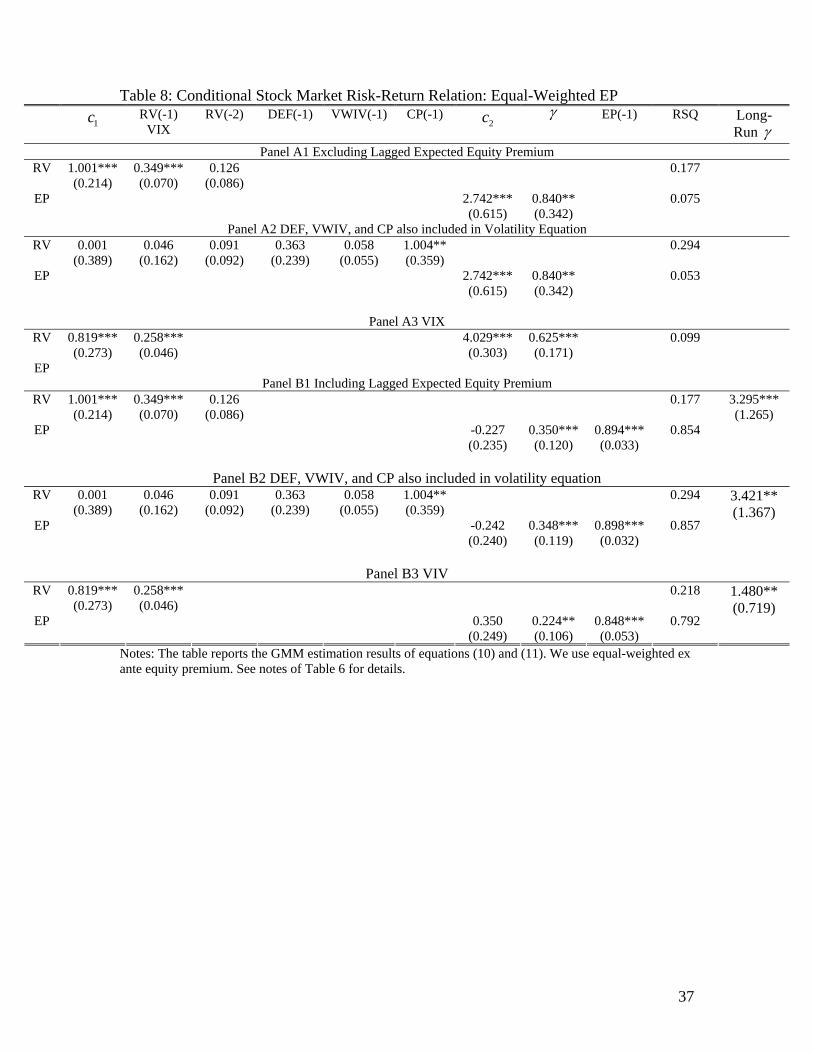
We also estimate equations (10) and (11) using equal-weighted EP and report the
results in Table 8. Again, for all specifications, γ , the coefficient of the risk-return
relation, is found to be positive and significant at the 5% level. The point estimates are
also similar to those reported in Table 6.
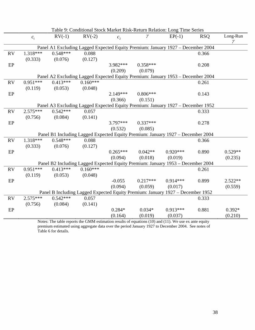
Thus far we have focused on the equity premium covering the 1975 to 1998
period. We focus more on the short time series because the equity premium is constructed
using firm-specific data. Here we finally examine the risk-return tradeoff using the long
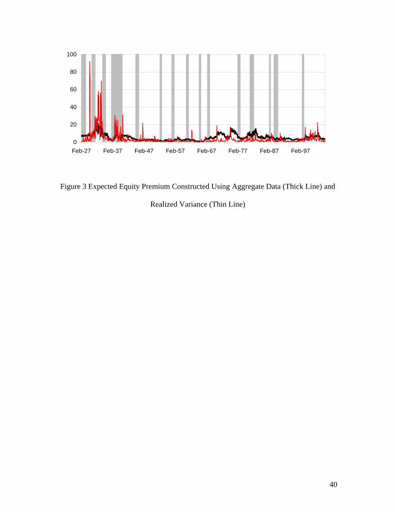
time series data covering the 1926 to 2004 period. As shown in Figure 3, the expected
return tends to increase during economic recessions.
We estimate equations (10) and (11) using the long time series data and report the
results in Table 9. To conserve space, we consider only the specification that the
conditional variance is a linear function of its two lags. Again, we find that γ is
significantly positive over the full sample (panels A1 and B1). To be robust, we also
consider two subsamples: January 1927 to December 1952 (panels A2 and B2) and
January 1953 to December 2004 (panels A3 and B3). The positive risk-return relation is
significant in both subsamples. We also examine the results using quarterly data and find
robust conclusions, to conserve space, they are not reported here but are available on
request.

24
VI. Conclusion
The intertemporal tradeoff between systematic equity market risk and expected
returns is one of the most important cornerstones in most asset pricing theories. The
empirical evidence, however, is rather mixed. In this paper, we argue that the conflicting
evidence stems from the fact that the expected equity market premium is not observable
and should be estimated. To illustrate this point, we investigate the risk-return relation in
the stock market using a measure of the ex ante expected stock market return. This
measure is forward-looking and does not rely critically on using realized equity returns or
instrumental variables. With such a measure, in contrast to many early authors, we find a
positive and significant risk-return tradeoff. Our results highlight the importance of using
the ex ante equity premium instead of the realized equity premium in asset pricing tests.
25
References:
Altman, E. I., and V. M. Kishore, 1998, Default and Returns of High Yield Bonds:
Analysis Through 1997, Unpublished Working Paper, New York University.
Andersen, T., T. Bollerslev, F. Diebold, and P. Labys, 2003, Modeling and Forecasting
Realized Volatility, Econometrica, 71, 579-625.
Brandt, M. and Q. Kang, 2004, On the Relationship Between the Conditional Mean and
Volatility of Stock Returns: A Latent VAR Approach, Journal of Financial Economics
72, 217-257.
Campbell, John, 1987, Stock Returns and the Term Structure, Journal of Financial
Economics, 18, 373-399.
Campbell, J. and J. Cochrane, 1999, By Force of Habit: a Consumption-Based
Explanation of Aggregate Stock Market Behavior, Journal of Political Economy, 107,
205-251.
Campbell, J., A. Lo, and C. MacKinlay, 1997, The Econometrics of Financial Markets,
Princeton University Press, Princeton, NJ.
Campbell, John, M. Lettau, B. Malkiel, and Y. Xu, 2001, Have Individual Stocks
Become More Volatile? An Empirical Exploration of Idiosyncratic Risk, Journal of
Finance, 56, 1-43.
Campbell, J. and G. Taksler, 2003, Equity Volatility and Corporate Bond Yield, Journal
of Finance, 58, pp. 2321-50.
Campbello, M., L. Chen, and L. Zhang, 2005, Expected Returns, Yield Spreads, and
Asset Pricing Tests, Unpublished Working Paper, Michigan State University.
Christensen, B., and N. Prabhala, 1998, The relation between implied and realized
volatility, Journal of Financial Economics, 50, 125-150.
26
Elton, E., 1999, Expected return, realized return, and asset pricing tests, Journal of
Finance, 54, 1199-1220.
Fama, E., and K. French, 1989, Business Conditions and Expected Returns on Stocks and
Bonds, Journal of Financial Economics, 25, 23-49.
French, K., G. Schwert, and R. Stambaugh, 1987, Expected stock returns and volatility,
Journal of Financial Economics, 19, 3-30.
Ghysels, E., P. Santa-Clara, and R. Valkanov, 2005, There is a risk-return tradeoff after
all, journal of Financial Economics, forthcoming.
Glosten, L., R. Jagannathan, and D. Runkle, 1993, On the relation between the expected
value and the variance of the nominal excess return on stocks, Journal of Finance, 48,
1779-1801.
Goyal, A. and P. Santa-Clara, 2003, Idiosyncratic Risk Matters!, Journal of Finance 58,
975-1007.
Graham, J. and C. Harvey, 2005, The Long-Run Equity Risk Premium, Unpublished
Working Paper, Duke University.
Guo, H., 2004, Limited Stock Market Participation and Asset Prices in a Dynamic
Economy, Journal of Financial and Quantitative Analysis, 39, 495-516.
Guo, H and R. Whitelaw, 2005, Uncovering the risk-return relation in the stock market,
Journal of Finance, forthcoming.
Huang, M. and J. Huang, 2003, How Much of the Corporate-Treasury Yield Spread is
due to Credit Risk?, Unpublished Working Paper, Stanford University.
Jones, P., S. Mason, and E. Rosenfeld, 1984, Contingent Claims Analysis of Corporate
Capital Structures: An Empirical Investigation, Journal of Finance, 39, 611-625.
27
Lettau, M. and S. Ludvigson, 2003, Measuring and Modeling Variation in the Risk-
Return Tradeoff, Unpublished Working Paper, Department of Economics, New York
University.
Merton, R., 1973, An Intertemporal Capital Asset Pricing Model, Econometrica, 41, 867-
887.
Merton, R., 1974, On the pricing of corporate debt: The risk structure of interest rates,
Journal of Finance, 29, 449-470.
Merton, R., 1980, On Estimating the Expected Return on the Market: An exploratory
Investigation, Journal of Financial Economics, 8, 323-361.
Pastor, L., M. Sinha, and B. Swaminathan, 2005, Estimating the intertemporal risk-return
tradeoff using the implied cost of capital, Unpublished Working Paper, University of
Chicago.
Pagan, A., 1984, Econometric Issue in the Analysis of Regressions with Generated
Regressors, International Economic Review, 25, 221-247.
Pindyck, R., 1984, Risk, inflation, and the stock market, American Economic Review,
74, 335-351.
Scruggs, J., 1998, Resolving the Puzzling Intertemporal Relation between the Market
Risk Premium and Conditional Market Variance: A Two-Factor Approach, Journal of
Finance, 53, 575-603.
Shiller, R., 1981, Do Stock Prices Move Too Much to be Justified by Subsequent
Changes in Dividends?, American Economic Review, 71, 421-436.
Whitelaw, R., 1994, Time variations and covariations in the expectation and volatility of
stock market returns, Journal of Finance, 49, 515-541.

28
Table 1: Summary Statistics
EP RET RV TERM RREL DEF DY EWIV VWIV CP VIX Panel A Univariate Statistics
Mean 3.84 10.21 1.97 1.81 -0.06 1.16 3.76 39.07 10.26 0.61 4.05 S.D. 2.07 51.81 1.73 1.30 1.38 0.8 1.10 16.71 3.76 0.38 3.06 AR(1) 0.93 0.04 0.32 0.94 0.82 0.97 0.99 0.71 0.53 0.81 0.79 ADF * *** *** *** ** *** *** *** ADF-T ** *** *** *** *** *** *** ***
Panel B Cross Correlation EP 1.00 RET 0.07 1.00 RV 0.20 -0.19 1.00 TERM 0.20 0.05 -0.10 1.00 RREL -0.40 -0.20 -0.11 -0.60 1.00 DEF 0.03 0.07 0.33 0.00 -0.30 1.00 DY -0.37 -0.07 0.20 -0.17 0.03 0.68 1.00 EWIV 0.57 0.01 0.27 0.23 -0.25 -0.22 -0.47 1.00 VWIV 0.32 -0.04 0.84 -0.07 -0.17 0.35 0.04 0.47 1.00 CP -0.06 -0.05 0.40 -0.05 0.04 0.32 0.36 -0.01 0.30 1.00 VIX 0.29 -0.34 0.76 -0.01 -0.13 0.35 0.14 0.28 0.65 0.55 1.00
Notes: EP is the value-weighted expected equity premium; RET is the realized equity premium; RV is the realized stock market variance; TERM is the term premium; RREL is the stochastically detrended risk-free rate; DEF is the default premium; DY is the dividend yield; EWIV is the equal-weighted idiosyncratic volatility; VWIV is the value-weighted idiosyncratic volatility; CP the yield spread between the commercial paper and 3-month Treasury bills; VIX is the end-of-month volatility implied from options written on S&P 100. VIX is available over the period January 1986 to March 1998; all the other variables are available over the period January 1975 to March 1998. ADF is the augmented Dick-Fuller unit root test with a constant and ADF-T is the augmented Dick-Fuller unit root test with a constant and a linear time trend. In the unit root tests, we choose the number of lags using the “general to specific” method recommended in Campbell and Perron (1991), with a maximum of six lags. ***, **, and * indicate that the null hypothesis of a unit root is rejected at the 1%, 5%, and 10% significance levels, respectively.
29
Table 2: Forecasting One-Month-Ahead Excess Stock Market Returns EP(-1) RV(-1) TERM(-1) RREL(-1) DEF(-1) DY(-1) EWIV(-1) VWIV(-1) CP(-1) RSQ
1 2.354 (1.477)
0.009
2 1.802 (1.802)
0.000
3 1.379 (2.315)
0.001
4 -5.677** (2.481)
0.023
5 2.547 (7.731)
0.001
6 -1.529 (3.062)
0.001
7 0.250 (0.179)
0.007
8 1.204* (0.705)
0.008
9 18.094* (10.768)
0.018
10 2.137* (1.492)
1.290 (1.845)
0.011
11 2.194 (1.509)
1.295 (2.285)
0.010
12 0.999 (1.652)
-5.101* (2.834)
0.025
13 2.314 (1.470)
5.026 (7.330)
0.011
14 2.769* (1.659)
2.110 (3.339)
0.011
15 1.777 (1.771)
0.126 (0.210)
0.010
16 1.844 (1.547)
0.883 (0.742)
0.013
17 2.516* (1.450)
14.885 (10.626)
0.021
18 6.187** (2.743)
0.009

30
Notes: This table reports the OLS regression results of forecasting one-month-ahead excess stock market returns. Newey-West standard errors estimated using four lags are reported in parentheses. ***, **, and * indicate significance at the 1%, 5% and 1% levels. EP is the value-weighted expected equity premium; RV is the realized stock market variance; TERM is the term premium; RREL is the stochastically detrended risk-free rate; DEF is the default premium; DY is the dividend yield; EWIV is the equal-weighted idiosyncratic volatility; VWIV is the value-weighted idiosyncratic volatility; CP the yield spread between the commercial paper and 3-month Treasury bills; VIX is the end-of-month volatility implied from options written on S&P 100. VIX is available over the period January 1986 to March 1998; all the other variables are available over the period January 1975 to March 1998. In row 18, we address the error-in-variable problem by using RREL, VWIV, and CP as instrumental variables for EP.

31
Table 3: Forecasting Realized Variance RV(-1) RV(-2) EP(-1) TERM(-1) RREL(-1) DEF(-1) DY(-1) EWIV(-1) VWIV(-1) CP(-1) VIX(-1) RSQ
1 0.322*** (0.086)
0.103
2 0.241*** (0.074)
0.249*** (0.067)
0.160
3 0.237*** (0.077)
0.246*** (0.064)
0.020 (0.039)
0.161
4 0.237*** (0.077)
0.247*** (0.069)
-0.057 (0.083)
0.162
5 0.236*** (0.077)
0.244*** (0.063)
-0.077 (0.070)
0.164
6 0.208** (0.086)
0.206*** (0.068)
0.527** (0.238)
0.178
7 0.230*** (0.080)
0.240*** (0.067)
0.111 (0.103)
0.165
8 0.251*** (0.074)
0.249*** (0.068)
-0.004 (0.005)
0.162
9 0.097 (0.126)
0.235*** (0.065)
0.083* (0.048)
0.169
10 0.161** (0.070)
0.185*** (0.067)
1.146*** (0.403)
0.210
11 -0.036 (0.128)
0.137** (0.070)
0.358* (0.210)
0.101** (0.049)
1.157*** (0.383)
0.233
12 0.219* (0.118)
0.318*** (0.073)
0.193
13 0.304*** (0.022)
0.280
14 -0.122 (0.171)
0.230*** (0.080)
1.114** (0.478)
0.157** (0.079)
0.806 (0.753)
0.235
15 -0.186** (0.086)
0.066 (0.087)
0.363*** (0.054)
0.300
16 -0.495*** (0.158)
-0.002 (0.080)
1.089** (0.498)
0.152** (0.071)
-0.164 (0.734)
0.385*** (0.073)
0.332
Notes: This table reports the OLS regression results of forecasting one-month-ahead realized stock market variance. Newey-West standard errors estimated using four lags are reported in parentheses. ***, **, and * indicate significance at the 1%, 5% and 1% levels. EP is the expected equity premium; RV is the realized stock market variance; TERM is the term premium; RREL is the stochastically detrended risk-free rate; DEF is the default premium; DY is the dividend yield; EWIV is the equal-weighted idiosyncratic volatility; VWIV is the value-weighted idiosyncratic volatility; CP the yield spread between the commercial paper and 3-month Treasury bills; VIX is the end-of-month volatility implied from options written on S&P 100. VIX is available over the period January 1986 to March 1998; all the other variables are available over the period January 1975 to March 1998.

32
Table 4: Expected Equity Premium and Lagged Realized Variance RV(-1) EP(-1) TERM(-1) RREL(-1) DEF(-1) DY(-1) EWIV(-1) VWIV(-1) CP(-1) RSQ
1 0.240** (0.095)
0.040
2 0.107*** (0.038)
0.921*** (0.031)
0.878
3 0.266*** (0.080)
0.348** (0.149)
0.088
4 0.109*** (0.039)
0.919*** (0.033)
0.017 (0.034)
0.878
5 0.191** (0.084)
-0.568*** (0.134)
0.183
6 0.108*** (0.038)
0.928*** (0.033)
0.023 (0.032)
0.878
7 0.254*** (0.096)
-0.157 (0.382)
0.042
8 0.117*** (0.042)
0.921*** (0.031)
-0.105 (0.097)
0.879
9 0.342*** (0.083)
-0.807*** (0.193)
0.216
10 0.118*** (0.040)
0.905*** (0.037)
-0.071 (0.046)
0.879
11 0.062 (0.077)
0.068*** (0.013)
0.324
12 0.086*** (0.026)
0.877*** (0.045)
0.011* (0.007)
0.883
13 -0.253 (0.163)
0.272*** (0.090)
0.114
14 0.032 (0.051)
0.911*** (0.030)
0.043** (0.020)
0.880
15 0.321*** (0.097)
-0.918 (0.526)
0.064
16 0.096** (0.039)
0.925*** (0.031)
0.124 (0.106)
0.879
17 0.240*** (0.074)
0.068*** (0.013)
0.324
18 0.115*** (0.032)
0.877*** (0.045)
0.011* (0.006)
0.883
19 0.240*** (0.089)
0.272*** (0.090)
0.114
20 0.110*** (0.038)
0.911*** (0.030)
0.043** (0.020)
0.880
33
Notes: This table reports the OLS estimation results of regressing the expected equity premium, EP, on lagged financial variables. Newey-West standard errors estimated using four lags are reported in parentheses. ***, **, and * indicate significance at the 1%, 5% and 1% levels. RV is the realized stock market variance; TERM is the term premium; RREL is the stochastically detrended risk-free rate; DEF is the default premium; DY is the dividend yield; EWIV is the equal-weighted idiosyncratic volatility; VWIV is the value-weighted idiosyncratic volatility; and CP the yield spread between the commercial paper and 3-month Treasury bills. To address the multicollinearity problem, in rows 15 through 18, we first regress EWIV or VWIV on RV and then use the residuals in the regression analysis.

34
Table 5: Granger Causality Tests EP(-1) EP(-2) RV(-1) RV(-2) RSQ GCT
1 EP 0.900*** (0.094)
0.030 (0.094)
0.123***(0.045)
-0.046 (0.037)
0.880
2 EP 0.917*** (0.096)
0.017 (0.093)
0.870 21.520***
3 RV -0.208** (0.083)
0.205** (0.086)
0.248***(0.073)
0.266***(0.068)
0.166
4 RV 0.241***(0.074)
0.248***(0.068)
0.158 2.607
Notes: We select lags using Schwarz Bayesian information criterion, with a maximum of six lags. White-corrected standard errors are reported in parentheses. ***, **, * denote significance at the 1%, 5%, and 10% levels, respectively. GCT is the Granger causality test statistic, which has a chi-squared distribution with two degrees of freedom.

35
Table 6: Conditional Stock Market Risk-Return Relation
1c RV(-1) VIX
RV(-2) DEF(-1) VWIV(-1) CP(-1) 2c γ EP(-1) RSQ Long-
Run γ Panel A1 Excluding Lagged Expected Equity Premium
RV 0.991*** (0.157)
0.241*** (0.074)
0.248*** (0.068)
0.158
EP 2.401*** (0.625)
0.732** (0.351)
0.051
Panel A2 DEF, VWIV, and CP also included in Volatility Equation RV -0.393
(0.372) -0.036 (0.128)
0.137* (0.071)
0.357* (0.211)
0.101** (0.049)
1.158*** (0.383)
0.231
EP 2.401*** (0.625)
0.732** (0.351)
0.021
Panel A3 VIX
RV 0.591*** (0.132)
0.304*** (0.022)
0.280
EP 3.898*** (0.345)
0.601*** (0.208)
0.086
Panel B1 Including Lagged Expected Equity Premium RV 0.991***
(0.157) 0.241*** (0.074)
0.248*** (0.068)
0.158
EP -0.328 (0.261)
0.341*** (0.128)
0.911*** (0.033)
0.869
3.826** (1.871)
Panel B2 DEF, VWIV, and CP also included in volatility equation
RV -0.393 (0.372)
-0.036 (0.128)
0.137* (0.071)
0.357* (0.211)
0.101** (0.049)
1.158*** (0.383)
0.231
EP -0.358 (0.269)
0.337*** (0.125)
0.921*** (0.032)
0.870
4.245* (2.315)
Panel B3 VIV
RV 0.591*** (0.132)
0.304*** (0.022)
0.280
EP 0.316 (0.286)
0.217* (0.111)
0.854*** (0.053)
0.783
1.484* (0.893)
Notes: The table reports the estimation results of equation system
(10) 1 1
2 1 1
( )[ ( )]
t t t
t t t
RV c f xEP c c f x
εγ ξ
−
−
= + += + + +
,
where 1c , 2c , and γ are parameters to be estimated, and tε and tξ are error terms. We consider three specifications for conditional stock market variance: It is a linear function of (1) two lags of realized variance; (2) two lags of realized variance and DEF, CP, and VWIV; and (3) VIX. We estimate the equation system (11) jointly using GMM. These results are reported in panels A1 through A3, respectively. In panel B, we also control for lagged EP in the conditional return equation:
(11) 1 1
2 1 1 1
( )[ ( )]
t t t
t t t t
RV c f xEP c c f x EP
εγ ρ ξ
−
− −
= + += + + + +
,
and report the GMM estimation results of equation (12) in panels B1 through B3. We use a constant and predictors of stock variance as instrument variables for the variance equation and a constant and one-period-lagged realized variance (and lagged EP in panel B) for the conditional return equation. Therefore,
the equation system is just identified. In panel B, the long-run γ is defined as 1γρ−
. ***, **, and *
denote significance at the 1%, 5%, and 10% levels.
36
Table 7: Expected Bond Premium and Lagged Realized Variance RV(-1) BP(-1) TERM(-1) RREL(-1) DEF(-1) DY(-1) EWIV(-1) VWIV(-1) CP(-1) RSQ
1 0.074*** (0.019)
0.075
2 0.024*** (0.006)
0.917*** (0.044)
0.884
3 0.076*** (0.019)
0.025 (0.032)
0.080
4 0.024*** (0.006)
0.919*** (0.045)
-0.005 (0.006)
0.884
5 0.064*** (0.017)
-0.118*** (0.026)
0.194
6 0.024*** (0.006)
0.924*** (0.049)
0.006 (0.008)
0.884
7 0.055*** (0.021)
0.207*** (0.077)
0.115
8 0.025*** (0.006)
0.921*** (0.047)
-0.014 (0.023)
0.884
9 0.082*** (0.020)
-0.062 (0.045)
0.096
10 0.025*** (0.006)
0.916*** (0.045)
-0.003 (0.007)
0.884
11 0.046** (0.018)
0.011** (0.004)
0.210
12 0.023*** (0.006)
0.907*** (0.404)
0.001 (0.001)
0.884
13 -0.013 (0.033)
0.048** (0.021)
0.120
14 0.015 (0.010)
0.912*** (0.043)
0.006 (0.004)
0.884
15 0.080*** (0.021)
-0.062 (0.112)
0.077
16 0.020*** (0.007)
0.921*** (0.044)
0.047** (0.024)
0.885
17 0.074*** (0.021)
0.011** (0.004)
0.210
18 0.025*** (0.006)
0.907*** (0.040)
0.001 (0.001)
0.884
19 0.074*** (0.018)
0.048** (0.021)
0.120
20 0.025*** (0.006)
0.912*** (0.043)
0.006 (0.004)
0.885
Notes: This table reports the OLS estimation results of regressing the expected bond premium, BP, on lagged financial variables. Newey-West standard errors estimated using four lags are reported in parentheses. ***, **, and * indicate significance at the 1%, 5% and 1% levels. RV is the realized stock market variance; TERM is the term premium; RREL is the stochastically detrended risk-free rate; DEF is the default premium; DY is the dividend yield; EWIV is the equal-weighted idiosyncratic volatility; VWIV is the value-weighted idiosyncratic volatility; and CP the yield spread between the commercial paper and 3-month Treasury bills.
37
Table 8: Conditional Stock Market Risk-Return Relation: Equal-Weighted EP
1c RV(-1) VIX
RV(-2) DEF(-1) VWIV(-1) CP(-1) 2c γ EP(-1) RSQ Long-
Run γ Panel A1 Excluding Lagged Expected Equity Premium
RV 1.001*** (0.214)
0.349*** (0.070)
0.126 (0.086)
0.177
EP 2.742*** (0.615)
0.840** (0.342)
0.075
Panel A2 DEF, VWIV, and CP also included in Volatility Equation RV 0.001
(0.389) 0.046
(0.162) 0.091
(0.092) 0.363
(0.239) 0.058
(0.055) 1.004** (0.359)
0.294
EP 2.742*** (0.615)
0.840** (0.342)
0.053
Panel A3 VIX
RV 0.819*** (0.273)
0.258*** (0.046)
4.029*** (0.303)
0.625*** (0.171)
0.099
EP
Panel B1 Including Lagged Expected Equity Premium RV 1.001***
(0.214) 0.349*** (0.070)
0.126 (0.086)
0.177
EP -0.227 (0.235)
0.350*** (0.120)
0.894*** (0.033)
0.854
3.295*** (1.265)
Panel B2 DEF, VWIV, and CP also included in volatility equation
RV 0.001 (0.389)
0.046 (0.162)
0.091 (0.092)
0.363 (0.239)
0.058 (0.055)
1.004** (0.359)
0.294
EP -0.242 (0.240)
0.348*** (0.119)
0.898*** (0.032)
0.857
3.421** (1.367)
Panel B3 VIV
RV 0.819*** (0.273)
0.258*** (0.046)
0.218
EP 0.350 (0.249)
0.224** (0.106)
0.848*** (0.053)
0.792
1.480** (0.719)
Notes: The table reports the GMM estimation results of equations (10) and (11). We use equal-weighted ex ante equity premium. See notes of Table 6 for details.
38
Table 9: Conditional Stock Market Risk-Return Relation: Long Time Series 1c RV(-1) RV(-2) 2c γ EP(-1) RSQ Long-Run
γ Panel A1 Excluding Lagged Expected Equity Premium: January 1927 – December 2004
RV 1.318*** (0.333)
0.548*** (0.076)
0.088 (0.127)
0.366
EP 3.982*** (0.209)
0.358*** (0.079)
0.208
Panel A2 Excluding Lagged Expected Equity Premium: January 1953 – December 2004 RV 0.951***
(0.119) 0.413*** (0.053)
0.160*** (0.048)
0.261
EP 2.149*** (0.366)
0.806*** (0.151)
0.143
Panel A3 Excluding Lagged Expected Equity Premium: January 1927 – December 1952 RV 2.575***
(0.756) 0.542*** (0.084)
0.057 (0.141)
0.333
EP 3.797*** (0.532)
0.337*** (0.085)
0.278
Panel B1 Including Lagged Expected Equity Premium: January 1927 – December 2004 RV 1.318***
(0.333) 0.548*** (0.076)
0.088 (0.127)
0.366
EP 0.265*** (0.094)
0.042** (0.018)
0.920*** (0.019)
0.890 0.529** (0.235)
Panel B2 Including Lagged Expected Equity Premium: January 1953 – December 2004 RV 0.951***
(0.119) 0.413*** (0.053)
0.160*** (0.048)
0.261
EP -0.055 (0.094)
0.217*** (0.059)
0.914*** (0.017)
0.899 2.522** (0.559)
Panel B Including Lagged Expected Equity Premium: January 1927 – December 1952 RV 2.575***
(0.756) 0.542*** (0.084)
0.057 (0.141)
0.333
EP 0.284* (0.164)
0.034* (0.019)
0.913*** (0.037)
0.881 0.392* (0.210)
Notes: The table reports the GMM estimation results of equations (10) and (11). We use ex ante equity premium estimated using aggregate data over the period January 1927 to December 2004. See notes of Table 6 for details.

39
0
0.5
1
1.5
2
1970 1975 1980 1985 1990 1995 2000
Figure 1 Annual Scaled Investment Grade (Solid Line) and Baa (Dashed Line) Default
Rates
0
4
8
12
Jan-
75
Jan-
77
Jan-
79
Jan-
81
Jan-
83
Jan-
85
Jan-
87
Jan-
89
Jan-
91
Jan-
93
Jan-
95
Jan-
97
Figure 2 Expected Equity Premium Constructed Using Firm-Level Data (Thick Line) and Realized Variance (Thin Line)
40
0
20
40
60
80
100
Feb-27 Feb-37 Feb-47 Feb-57 Feb-67 Feb-77 Feb-87 Feb-97
Figure 3 Expected Equity Premium Constructed Using Aggregate Data (Thick Line) and
Realized Variance (Thin Line)