IEF

EIEF Working Paper 23/10

December 2010

Commodity Money with Frequent Search

by

Ezra Oberfield

(Federal Reserve Bank of Chicago)

Nicholas Trachter

(EIEF)

EIE

F

WO

RK

ING

P

AP

ER

s

ER

IEs

E i n a u d i I n s t i t u t e f o r E c o n o m i c s a n d F i n a n c e

Commodity Money with Frequent Search∗

Ezra Oberfield

Federal Reserve Bank of Chicago

ezraoberfield@gmail.com

Nicholas Trachter

EIEF

nicholas.trachter@eief.it

November 16, 2010

Abstract

A prominent feature of the Kiyotaki and Wright (1989) model of commodity moneyis the multiplicity of dynamic equilibria. We show that the frequency of search isstrongly related to the extent of multiplicity. To isolate the role of frequency of searchin generating multiplicity, we (i) vary the frequency of search without changing thefrequency of finding a trading partner and (ii) focus on symmetric dynamic equilibria,a class for which we can sharply characterize several features of the set of equilibria.For any finite frequency of search this class retains much of the multiplicity. For eachfrequency we characterize the full set of equilibrium payoffs, strategies played, anddynamic paths of the state variables. Indexed by any of these features, the set ofequilibria converges uniformly to a unique equilibrium in the continuous search limit.We conclude that when search is frequent, the seemingly exotic dynamics are irrelevant.

KEYWORDS: Commodity Money, Search, Multiple Equilibria, Sunspots.

∗First version: March 2010. This paper previously circulated as “Period Length and the Set ofEquilibria with Commodity Money.” We thank Fernando Alvarez, Marco Bassetto, Jarda Borovicka,Jan Eeckhout, Lars Hansen, Ricardo Lagos, Stephen Morris, Robert Shimer, Andy Skrzypacz, NancyStokey, Aleh Tsyvinski, and Randall Wright for useful comments. We also benefited from commentsby seminar and conference participants at Einaudi Institute for Economics and Finance (EIEF),Federal Reserve Bank at Boston, Summer Workshop on Money, Banking, Payments, and Finance(2010), University of Chicago, Universidad Torcuato Di Tella (UTDT), and Vienna MacroeconomicsWorkshop 2010. The views expressed herein are those of the authors and not necessarily those ofthe Federal Reserve Bank of Chicago or the Federal Reserve System. All mistakes are our own.

1 Introduction

In their seminal contribution, Kiyotaki and Wright (1989) introduced a search the-

oretic model of commodity money in which goods can function as a medium of ex-

change, sparking a voluminous literature exploring the microfoundations of money.

Characterizing the set of dynamic equilibria is an essential part of many applica-

tions. These models feature a large multiplicity of dynamic equilibria that includes

cycles, sunspots, and other non-Markovian equilibria. While multiplicity is in some

sense a natural feature of monetary models, it can also make analyzing dynamics a

challenging task.

This paper demonstrates the tight connection between the extent of multiplicity

and the frequency of search. We adapt the model parameters so that one can vary

the frequency of search without altering other features of the economy such as the

frequency of actually meeting trading partners in a given unit of time. Agents search

each period, but are less likely to find a trading partner if the time period is short. By

varying the period length, we can study economies with different search frequencies.

We focus on the set of symmetric equilibria in an economy with symmetric param-

eters and initial conditions. Within this class of equilibria, the role of the frequency

of search is especially stark. With any strictly positive interval between search oppor-

tunities, the set of symmetric equilibria retains much of the multiplicity. In contrast,

in the limiting case in which agents search continuously there is a unique dynamic

equilibrium.

The fact that there are multiple equilibria with any strictly positive interval be-

tween search opportunities but a unique equilibrium with continuous search can give

the impression that there is a qualitative difference between the two. If the relevant

interval between search opportunities is indeed positive, one might think that a model

1

with continuous search may be ignoring potentially interesting and relevant dynam-

ics.1 We show that despite the qualitative difference, the unique equilibrium of the

continuous search limit is a good approximation to every equilibrium when search is

frequent.

We characterize the set of payoffs consistent with a symmetric equilibrium for all

points in the state space. The size of this set varies directly with the probability of

meeting a trading partner within a single period, decreasing monotonically as search

becomes more frequent. While we cannot characterize the strategies played within

any particular period, we show that the average strategy played within any interval

of time converges uniformly to the strategies of the continuous search limit. Lastly,

we show that the set of equilibrium paths of the economy converges uniformly to the

equilibrium path of the continuous search limit. These results imply that if search is

frequent, all dynamic equilibria are well approximated by the unique equilibrium of

the continuous search limit.

The connection between multiplicity and frequency of search is a subtle one. To get

at this relationship, we first describe the forces driving strategic decisions. Commodity

money arises because there is no double coincidence of wants. An individual may be

willing to trade for a commodity hoping to later meet a trading partner who desires

that commodity.

Individuals’ strategies of whether to accept commodity money are linked tem-

porally. If those who produce the good that agent j wants will not be accepting

commodity money (the good j produce) in the future, then there is a stronger in-

1Carlstrom and Fuerst (2001) write ”...as monetary theorists we must be careful in writing thebasics of our models... continuous-time analysis simply sweep this fundamental issue under therug... Since these indeterminacy issues arise for any discrete but arbitrarily small time period thisresolution of the timing is artificial.” Carlstrom and Fuerst (2001) were discussing how the timingassumptions of purchases requiring cash (whether real balances before or after purchases enter theutility function) affect determinacy with various interest rate rules. Fudenberg and Levine (2009)show games of imperfect monitoring are another context in which the distinction between discreteand continuous time is important.

2

centive for j to trade for commodity money (the good the others want) now. In this

sense, trading for commodity money in one period and others not accepting it in

future periods (and vice versa) are strategic complements. This provides the key to

understanding the source of multiplicity.

The strategic complementarity weakens as search becomes more frequent. When

search is infrequent, agents are more likely to trade within each period, so the strategy

played within a single period has more influence on payoffs in subsequent periods. As

a consequence, less frequent search corresponds to stronger complementarities, and

hence a larger set of equilibria.

Continuous search is special in that the complementarities disappear completely.

Stated differently, for there to be multiple equilibria there must be negative serial

correlation in trading strategies. Just as there cannot be negative serial correlation

in continuous time, there cannot be negative serial correlation when agents search

continuously.

Our contribution is threefold. First, we point to little understood features of

a model that has served as a blueprint for the extensive literature exploring the

microfoundations of money. Many recent models share properties with the Kiyotaki

and Wright (1989) model, and multiplicity comes from the same sources. While

multiplicity is an important feature of these models, we paint a more full picture of

the forces driving it. Second, for this class of models, we provide reassurance that

when agents have frequent opportunities to search, little is lost when writing the

model with agents searching continuously, as the dynamic equilibria of the discrete

versions are well approximated by the continuous search model. This is useful because

characterizing dynamics under continuous search can be considerably easier than

in the discrete counterparts, especially in applications such as the evolution of an

economy following the introduction of fiat money or changes in the quantity of money.

Third, we make a methodological contribution by providing an approach to studying

3

several features of the set of dynamic equilibria using easily accessible tools.

Our results are related to the findings of Abreu, Milgrom, and Pearce (1991), who

study a continuously repeated prisoner’s dilemma with imperfect monitoring. In that

model, lengthening the period over which actions are held fixed increases the possibil-

ities for cooperation, expanding the set of feasible equilibrium payoffs. Similarly, in a

model of commodity money with infrequent search, the fact that strategies are held

fixed for an entire period is a key feature that drives the large multiplicity of equilib-

ria. While the game studied by Abreu, Milgrom, and Pearce (1991) is purely a game

of coordination, the Kiyotaki and Wright (1989) model is an anonymous sequential

game (see Jovanovic and Rosenthal (1988)) in which strategic concerns play no role.

There are strategic complementarities that are inherently intertemporal, driven by

real changes in the distribution of holdings.

The relationship between period length and determinacy has also arisen in the real

business cycle literature. Several departures from the standard growth model lead

to indeterminacy (see Benhabib and Farmer (1999)). In some of these models, the

continuous time limit features a unique equilibrium. While superficially similar, these

and the Kiyotaki and Wright (1989) models have disparate sources of multiplicity,

and consequently the relationship between period length and multiplicity differ. In

versions of the RBC model with external effects that generate increasing returns, there

is typically a critical period length period length below which multiplicity disappears.2

Determinacy for a short enough time period (i.e., large enough discount factor) is

also a property of growth models that use an overlapping generations framework.3 In

contrast, in the Kiyotaki and Wright (1989) model, there is a continuum of dynamic

equilibria for any positive period length.

Section 2 lays out the economic environment while Section 3 describes symmetric

2See Hintermaier (2005).3See Boldrin and Montrucchio (1986).

4

equilibria. Section 4 gives examples of the many types of equilibria that can arise

and shows that these exist for any finite frequency of search. Section 5 contains our

main results: we characterize the set of perfect foresight equilibria and show how this

varies with the frequency of search. Section 6 extends these results to include sunspot

equilibria and we conclude in Section 7.

2 Model

There are three types of goods, labeled 1, 2, and 3, and a unit mass of infinitely lived

individuals that specialize in consumption and production. There are three types of

individuals, with equal proportions, indexed by the type of good they produce and

like to consume: an individual of type i derives utility only from consuming good

i, and produces only good i + 1 (mod 3). Goods are indivisible and storable, but

individuals can only store one good (and hence one type of good) at a time. Storage

is costless.4

Time is discrete with h being the length of time elapsed between periods. Each

period, individuals search for trading partners. Search is successful with probability

α(h).5 When an individual finds a potential trading partner, the two may exchange

goods. If a type i individual is able to acquire and consume good i, she derives

instantaneous utility u > 0. Immediately after consumption she produces a new unit

of good i+ 1.

When two individuals meet, it will never be the case that each desires the good

produced by the other. Even though there is never a double coincidence of wants, an

4Kiyotaki and Wright (1989) allow for storage costs to vary by good and by type. We willeventually specialize to a symmetric economic environment in which the storage cost is the same forall goods. In that environment the level of the storage cost is not relevant for any economic decisionsor outcomes, so we avoid the extra notation by setting the storage cost to 0.

5If α(h) ≈ α0h then the frequency of meeting a potential trading partner in a given unit of timeis roughly independent of h. We leave the functional form unspecified for greater generality.

5

individual may accept a good that she does not want to consume in order to exchange

it later for the good she desires. In this way, the intermediate good acts as a medium

of exchange.

Individuals discount future flows with the discount factor β(h) < 1. We assume

that β(h) is strictly decreasing and that limh↓0 β(h) = 1 (e.g. β(h) = e−rh). In

addition, we assume that α(h) is strictly increasing, and that limh↓0α(h)h

= α0 so that

the continuous time limit is well defined.

Let I = 1, 2, 3 be both the set of goods and the set of types, and T = nh∞n=0

denote the set of times when individuals can search.

2.1 Strategies and Equilibrium

A strategy for individual i is a function τ i : I2 → 0, 1, where τ i(j, k) = 1 if i

wants to trade good j for good k and τ i(j, k) = 0 otherwise. Following Kiyotaki and

Wright (1989) and Kehoe, Kiyotaki, and Wright (1993) we make the following two

assumptions. First we assume that τ i(j, k) = 1 if and only if τ i(k, j) = 0, so that if

an individual trades j for k she will not trade k for j. This ensures that an agent’s

preferences between the good they produce and commodity money are independent

of the good they are currently holding. Second, we assume that in a given period,

agents of the same type choose the same (potentially mixed) trading strategy. This

ensures that the agent’s willingness to exchange good j for k is independent of the

type, and holdings of the potential trading partner.6

Since u > 0, individuals will always want to trade for their desired good, so that

τ i(j, i) = 1 for all j. Given this, a strategy can be summarized by τ i(i + 1, i + 2),

6These assumptions are not without loss of generality. If the agents strictly prefer either the goodthey produce or commodity money, then these assumptions would in fact be equilibrium outcomes;when agents are indifferent, there is no reason for these assumptions to hold. One could easily relaxthe assumptions, but at the cost of more cumbersome notation. Since we will eventually focus onsymmetric equilibria, additional generality at this point adds nothing of substance to our analysis.

6

an agent’s willingness to trade the good she produces for commodity money. Let si

be the probability that type i wants to trade for commodity, i.e., plays the strategy

τ i(i+ 1, i+ 2) = 1.

There may be equilibria in which individuals coordinate their actions using the

realizations of a sunspot variable. Let xtt∈T be an exogenous sequence of random

variables that are independent across time and uniformly distributed in the [0, 1]

interval. Let sit be the strategy played by type i at time t. A history at the beginning

of the period at time t, denoted by zt, can be written as

zt =si0, ..., s

it−hi∈I ;x0, ..., xt

with zt ∈ Zt = [0, 1]3

th

+( th+1).

A strategy for an individual is a sequence of functions sit : Zt → [0, 1], giving the

trading strategy for each possible history.

Type i will never store good i; upon acquiring it, she immediately consumes it

and produces a new unit of good i + 1. Let pit : Zt−h → [0, 1] denote the fraction of

individuals of type i storing good i+1 at the beginning of the period at time t following

the history zt−h. The distribution of inventories at a point in time can be completely

summarized by the vector Pt (zt) ≡ pit (zt)i∈I . Given the trading strategies used at

time t, sit (zt)i∈I , we can derive an equation describing the evolution of inventories

from t to t+ h.

Following the accounting convention of Kiyotaki and Wright (1989), let V i,jt :

Zt → R denote the present discounted value for type i storing good j at the end of

the period at time t for a given history. Given i’s strategies, sitt∈T, the strategies

of others, siti∈I,t∈T, and an initial condition, P0, V i,jt is well defined.7 We can write

7As this is an anonymous sequential game, reputation and other strategic concerns play no role.

7

V i,jt (zt) as:

V i,jt

(zt)

= maxsit+nh

∞n=1

E

∞∑n=1

β(h)nuIut+nh

∣∣∣∣∣ zt

(1)

The expectation operator accounts for the uncertainty of meeting trading partners

and realizations of the sunspot variable xt, and Iut is an indicator of whether the

individual consumes her good at time t.

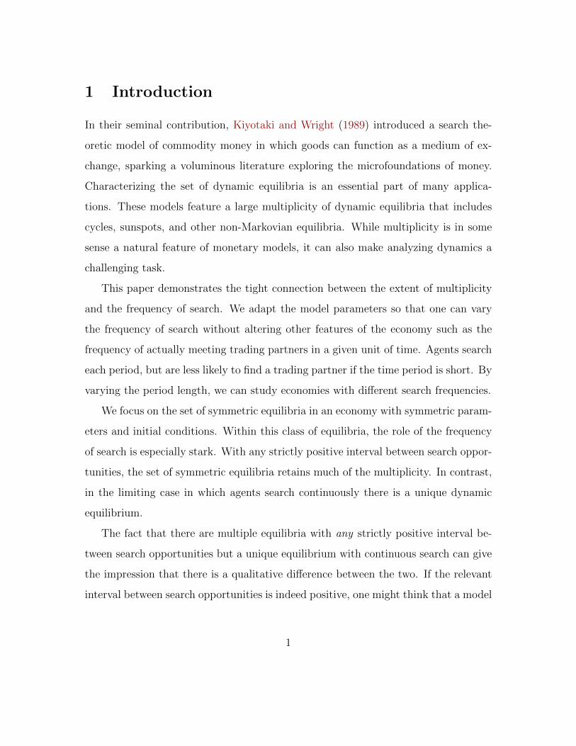
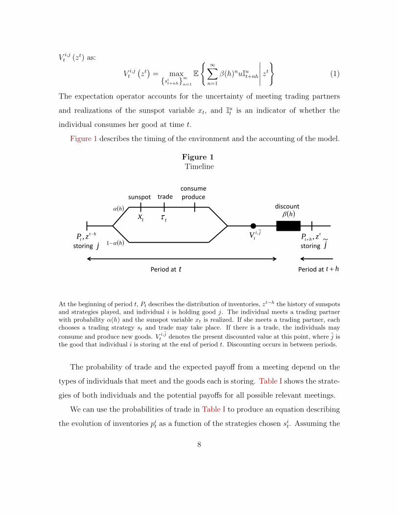
Figure 1 describes the timing of the environment and the accounting of the model.

Figure 1Timeline

consume

h h

tradeconsumeproduce

discountsunspot

x

htt zP ,

jji

tV~, t

ht zP ,j~

h1

t

storing storing

tx

j j

t

storing storing

Period at ht Period at

At the beginning of period t, Pt describes the distribution of inventories, zt−h the history of sunspotsand strategies played, and individual i is holding good j. The individual meets a trading partnerwith probability α(h) and the sunspot variable xt is realized. If she meets a trading partner, eachchooses a trading strategy st and trade may take place. If there is a trade, the individuals may

consume and produce new goods. V i,jt denotes the present discounted value at this point, where j isthe good that individual i is storing at the end of period t. Discounting occurs in between periods.

The probability of trade and the expected payoff from a meeting depend on the

types of individuals that meet and the goods each is storing. Table I shows the strate-

gies of both individuals and the potential payoffs for all possible relevant meetings.

We can use the probabilities of trade in Table I to produce an equation describing

the evolution of inventories pit as a function of the strategies chosen sit. Assuming the

8

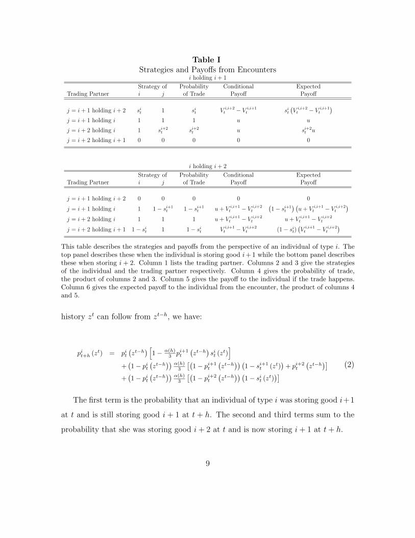
Table IStrategies and Payoffs from Encounters

i holding i+ 1

Strategy of Probability Conditional ExpectedTrading Partner i j of Trade Payoff Payoff

j = i+ 1 holding i+ 2 sit 1 sit V i,i+2t − V i,i+1

t sit(V i,i+2t − V i,i+1

t

)j = i+ 1 holding i 1 1 1 u u

j = i+ 2 holding i 1 si+2t si+2

t u si+2t u

j = i+ 2 holding i+ 1 0 0 0 0 0

i holding i+ 2

Strategy of Probability Conditional ExpectedTrading Partner i j of Trade Payoff Payoff

j = i+ 1 holding i+ 2 0 0 0 0 0

j = i+ 1 holding i 1 1− si+1t 1− si+1

t u+ V i,i+1t − V i,i+2

t

(1− si+1

t

) (u+ V i,i+1

t − V i,i+2t

)j = i+ 2 holding i 1 1 1 u+ V i,i+1

t − V i,i+2t u+ V i,i+1

t − V i,i+2t

j = i+ 2 holding i+ 1 1− sit 1 1− sit V i,i+1t − V i,i+2

t (1− sit)(V i,i+1t − V i,i+2

t

)This table describes the strategies and payoffs from the perspective of an individual of type i. Thetop panel describes these when the individual is storing good i+ 1 while the bottom panel describesthese when storing i + 2. Column 1 lists the trading partner. Columns 2 and 3 give the strategiesof the individual and the trading partner respectively. Column 4 gives the probability of trade,the product of columns 2 and 3. Column 5 gives the payoff to the individual if the trade happens.Column 6 gives the expected payoff to the individual from the encounter, the product of columns 4and 5.

history zt can follow from zt−h, we have:

pit+h (zt) = pit(zt−h

) [1− α(h)

3 pi+1t

(zt−h

)sit (zt)

]+(1− pit

(zt−h

)) α(h)3

[(1− pi+1

t

(zt−h

)) (1− si+1

t (zt))

+ pi+2t

(zt−h

)]+(1− pit

(zt−h

)) α(h)3

[(1− pi+2

t

(zt−h

)) (1− sit (zt)

)] (2)

The first term is the probability that an individual of type i was storing good i+1

at t and is still storing good i + 1 at t + h. The second and third terms sum to the

probability that she was storing good i+ 2 at t and is now storing i+ 1 at t+ h.

9

We can also rewrite the sequential problem in equation (1) with a recursive repre-

sentation. For an individual of type i, there are two relevant cases, one for each good

that would be stored. The value of storing good i+ 1 is,

V i,i+1t (zt) = β(h)EV i,i+1

t+h + α(h)3

[pi+1t+hs

it+h(V

i,i+2t+h − V

i,i+1t+h )

+(1− pi+1t+h)u+ pi+2

t+hsi+2t+hu]|zt

(3)

while the value of holding i+ 2 is

V i,i+2t

(zt)

= β(h)EV i,i+2t+h + α(h)

3

[(1− pi+1

t+h

) (1− si+1

t+h

) (u+ V i,i+1

t+h − V i,i+2t+h

)+pi+2

t+h

(u+ V i,i+1

t+h − V i,i+2t+h

)+(1− pi+2

t+h

) (1− sit+h

) (V i,i+1t+h − V i,i+2

t+h

)]|zt (4)

Here we suppressed the arguments of pit+h, sit+h, and V i,j

t+h, and the expectation is

taken only over realizations of the sunspot variable xt+h.

If holding good i + 1 is more valuable than holding i + 2, the strategy si = 0

is optimal (and si = 1 for the opposite case). If holding either good is equally

valuable then any strategy can be optimal. Define ∆it : Zt → R so that ∆i

t (zt) ≡

V i,i+1t (zt)− V i,i+2

t (zt). ∆i denotes the difference in value between storing i + 1 and

storing i + 2, or equivalently the gain from exchanging i + 2 for i + 1. An optimal

trading strategy sit therefore satisfies

sit(zt)∈

0 if ∆i

t (zt) > 0

[0,1] if ∆it (zt) = 0

1 if ∆it (zt) < 0

(5)

We now define an equilibrium.

Definition 1 For an initial condition, P0, an equilibrium is a sequence of inventories

10

pit, trading strategies sit, and value functions V i,i+1t , V i,i+2

t denoted by

pit, s

it, V

i,i+1t−h , V i,i+2

t−ht∈T,i∈I

such that (i) equations (2), (3), (4), and (5) are satisfied, and (ii) the transversality

conditions limt→∞ E−h[β(h)t/hV i,j

t

]= 0 holds for all i, j.

3 Symmetric Equilibria

We focus on symmetric equilibria in a symmetric environment: given a symmetric

initial condition P0 = p0, p0, p0, we study equilibria in which trading strategies

are symmetric (sit = st for all i) and as a consequence inventories remain symmetric

(pit = pt for all i). In this case, the evolution of inventories in equation (2) reduces to

pt+h (zt) = pt(zt−h

)− α(h)

3p2t

(zt−h

)st (zt)

+α(h)3

(1− pt

(zt−h

)) [2(1− pt

(zt−h

))(1− st (zt)) + pt

(zt−h

)] (6)

and the evolution of ∆t is

∆t

(zt)

= β(h)E

∆t+h + α(h)3u[st+h − pt+h]

−α(h)3

[pt+hst+h + 2(1− pt+h)(1− st+h) + pt+h]∆t+h

∣∣∣∣∣∣ zt (7)

The following lemma will assist in the characterization of equilibria. Of particular

use, we show that if ∆tt∈T corresponds to value functions that satisfy the sequence

problem, then it must have a uniform bound.

Lemma 1 Given an initial condition p0, a sequence pt, st,∆t−ht∈T represents a

symmetric equilibrium if and only if (i) equations (5), (6), and (7) are satisfied and,

(ii) there exists B > 0 such that for every t, Pr∣∣∆t−h

(zt−h

)∣∣ ≤ B

= 1.

11

Proof. See Appendix A.

Lemma 1 implies that we can look for equilibria in the space pt, st,∆t−ht∈T.

3.1 Symmetric Steady State Equilibrium

In this section we show existence and uniqueness of symmetric steady state equilibria.

Kehoe, Kiyotaki, and Wright (1993) shows that with asymmetric storage costs there

are a finite number of steady state equilibria. We show that with symmetric costs

there is a unique symmetric steady state.

In any steady state equilibriumpt(zt−h

), st (zt) ,∆t−h

(zt−h

)= pss, sss,∆ss

for all t ∈ T and zt ∈ Zt. In this case equation (7) can be rearranged to get

∆ss =u [sss − pss]

1−β(h)β(h)

[α(h)

3

]−1

+ pss + 2(1− pss)(1− sss) + pss

Since the denominator is positive, the value of ∆ss and hence the optimal trading

strategy sss depend on the sign of sss−pss. Consider first the possibility that ∆ss < 0:

this would imply sss = 1 and hence ∆ss ≥ 0, a contradiction. Consider next ∆ss > 0:

this would imply sss = 0 and hence ∆ss ≤ 0, also a contradiction. The only remaining

possibility is ∆ss = 0 which holds if and only if sss = pss which would be consistent

with the optimal choice of the trading strategy given in equation (5). Using the

evolution of inventories, equation (6), together with pt = st = pss for all t ∈ T

provides pss = sss = 23.

3.2 The Zero Equilibrium

We next consider a special dynamic equilibrium and label it the the Zero Equilibrium.

As we will show below, an equilibrium of this type will be the unique surviving equi-

librium as the interval between search opportunities, h, goes to zero. The strategies

12

of the Zero Equilibrium will also be helpful in characterizing the set of equilibria for

any fixed h.

For any h, there exists a unique equilibrium for which ∆t (zt) = 0 for all t, zt.

This equilibrium is Markovian, and the strategy played is always st = pt. This

condition implies that the probability of being able to obtain the desired good within

the period is independent of the good the agent is currently holding.8 It is easy to

see that equation (5) and equation (7) are both satisfied. For any initial condition p0,

one can find the sequence of inventories by iterating equation (6). Such a sequence

pt, st,∆t−ht∈T satisfies the conditions of Lemma 1 and is therefore an equilibrium.

We construct the Zero Equilibrium by finding a sequence of strategies and inven-

tories so that individuals are indifferent between accepting and rejecting commodity

money every period. When choosing a current strategy, individuals are concerned

with three quantities: the fraction of people holding the commodity money; the strate-

gies chosen by others; and the future relative value of holding commodity money. In

the Zero Equilibrium, the future relative value is zero by construction. If a larger

fraction of people are holding the good they produce (p ↑), trading for commodity

becomes more advantageous. If others are more willing to accept commodity money

(s ↑), there is less of a need to accept commodity money; others will accept the

produced good in exchange for the desired good. In the Zero Equilibrium these two

forces balance perfectly: when fewer people hold commodity money, more are willing

to accept it.

The same logic explains why there is a unique symmetric steady state, as this is

the Zero Equilibrium for a particular initial condition.

8If individual 1 is holding good 2 her probability of trading for good 1 with a type 2 is 1−p2 andwith type 3 is p3s3, so that the probability of trading for the desired good is 1 − p2 + p3s3. If theindividual 1 is holding good 3 her probability of trading for good 1 with a type 2 is (1− p2)(1− s2)and with type 3 is p3, so that the probability of trading for the desired good is (1− p2)(1− s2) + p3.In a symmetric equilibrium these values are equated when s = p.

13

4 Indeterminacy

In this section we provide examples of several types of equilibria. We show that

for a fixed frequency of search, there is a large multiplicity of dynamic equilibria.

Several examples are taken from Kehoe, Kiyotaki, and Wright (1993), who worked

with a model with asymmetric parameters and allow for asymmetric strategies. The

purpose of this section is to demonstrate that many of these types equilibria are still

present in an environment with symmetric parameters, even with the restriction of

symmetric strategies.

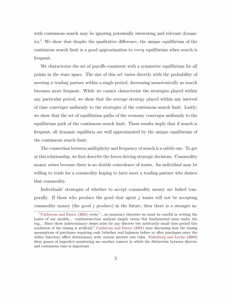
First we provide examples of deterministic equilibria that eventually converge to

the steady state. Figure 2 shows the evolution of the trading strategy s and inventories

p as a function of the elapsed time t for a particular equilibrium. The economy starts

with p0 = pss. We are interested in rationalizing an equilibrium with s0 > sss.

Since some traders will be acquiring commodity money, the fraction of individuals

holding their own produced good falls, ph < pss. From period h onward, the traders

play the strategies of the Zero Equilibrium. Each period, s and p move together,

balancing the incentives to accept and reject commodity money. At the end of the

initial period, these incentives are also balanced, regardless of the high value of the

initial trading strategy, s0.9 Therefore this is, indeed, an equilibrium. In fact, any s0

can be rationalized by playing sh = ph and then following the strategies of the Zero

Equilibrium.

This argument can be formalized and generalized. Notably, the argument is in-

dependent of the initial value of p0 and, given a particular p0, the initial strategy

chosen, s0. Given the initial condition p0, choose any s0. This gives ph. From ph

9It is true that both the trading strategy during the initial period and the lower fraction ofindividuals holding their own good in future periods make commodity money less useful during theinitial period. But the only implication of this is that coming into the initial period, traders wouldhave preferred to have been holding their own produced good, ∆−h > 0.

14

Figure 2Rationalizing Deterministic Equilibrium Paths

ssss sp

s

p sp

t0 h h2

An example of a deterministic equilibrium that converges to the steady state.

there exists strategies consistent with equilibrium such that ∆t = 0 for all t ∈ T

(the strategies of the Zero Equilibrium). Since ∆0 = 0 the choice of s0 is optimal, a

fact that is independent of the value of ∆−h. Because the choice of s0 was arbitrary,

each different s0 corresponds to a different dynamic equilibrium. There is therefore a

continuum of such deterministic dynamic equilibria.10

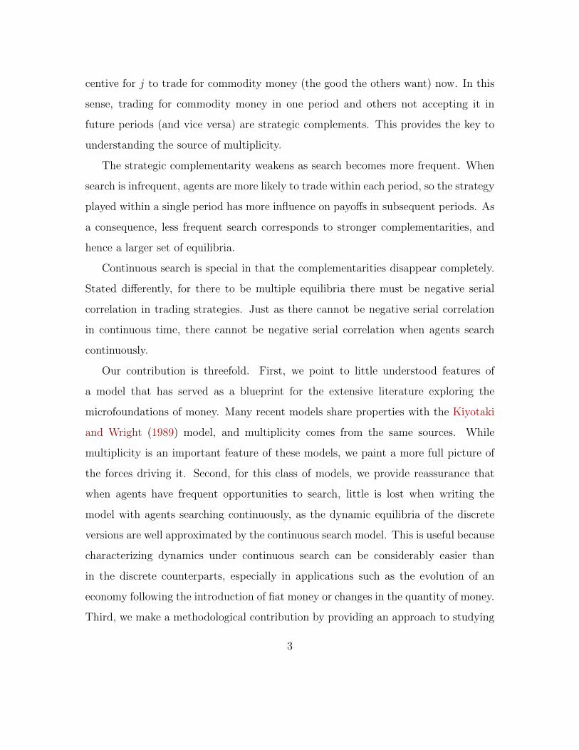
We can also construct cyclical equilibria. We provide an example for the following

parametrization: α(h) = 0.1, β(h) = 0.98, and u = 1. The economy cycles between

two triplespnh, snh,∆(n−1)h

. When n is odd the economy lies at 0.6737, 1, 0, and

lies at 0.6659, 0.3174,−0.0114 when n is even. In contrast to the Zero Equilib-

rium, cyclical equilibria are rationalized by the balance between current and future

incentives. In odd periods, more traders are willing to accept commodity money and

more are holding their own good. Both of these make it easy to get the desired good

using only the produced good, reducing the relative value of commodity money. In

10The idea for this type of equilibrium originates with a construction by Aiyagari and Wallace(1992) with fiat money.

15

even periods, it becomes harder to get the desired good using the produced good,

increasing the relative value of commodity money. These cycles persist as the period

length shrinks, a claim that we formalize in Appendix B.

Figure 3Example of a cyclical equilibrium

O

pO

E

The equilibrium is characterized by pt, st,∆t−h. In this case: E = 0.6659, 0.3174,−0.0114 andO = 0.6737, 1, 0. Parametrization: α(h) = 0.1, β(h) = 0.98 and u = 1.

Finally, we can also construct non-Markovian equilibria, combining the two previ-

ous examples. For the first 2N − 1 periods, individuals play the strategies associated

with the cyclical equilibrium described above. From period 2N on, all individuals

play the strategies associated with the Zero Equilibrium, so that ∆t = 0. In fact, we

can construct an equilibrium in which every odd period the realization of the sunspot

x(2n+1)h determines whether the individuals continue to play the cyclical strategies or

the economy reverts to the Zero Equilibrium.

5 Perfect Foresight Equilibria

In this section we discuss perfect foresight equilibria. While individuals still face

uncertainty in terms of meeting trading partners, pt, st and ∆t are no longer functions

of the sunspot variables xt and follow deterministic paths. We can therefore drop

16

the expectation operator in equation (7).

5.1 Continuous Search

The dynamics of the limiting model in which agents search continuously are simple

and easy to describe. There is a unique equilibrium, in which agents choose st = pt

for all t > 0.

For the continuous time model to be well defined, recall that we assume the

following limits exist: Let r = limh↓01h

(1

β(h)− 1)

be the instantaneous discount rate

and α0 = limh↓0α(h)h

be the instantaneous meeting rate.

As h → 0, we approach the continuous search limit. Using equation (6) and

equation (7) we can show that pt and ∆t exist and satisfy:

pt =α0

3

[−p2

t st + (1− pt) (2(1− pt)(1− st) + pt)]

(8)

and

r∆t = ∆t +α0

3u [st − pt]−

α0

3[ptst + 2(1− pt)(1− st) + pt] ∆t (9)

It is straightforward to show the only symmetric equilibrium is the Zero Equilib-

rium, i.e., ∆t = 0 for all t ≥ 0 and the optimal strategy must be st = pt. One can

extend the definition of symmetric equilibrium and Lemma 1 to the continuous case

and show that for any equilibrium, ∆tt≥0 must have a uniform bound. First, note

that ∆t > 0 implies ∆t > r∆t and similarly ∆t < 0 implies ∆t < r∆t. Together,

these imply that if there is a t at which ∆t 6= 0 then |∆| will grow exponentially and

without bound, violating Lemma 1. Lastly, observe that if ∆t = 0, it must be that

st = pt for almost every t. These dynamics are summarized by the phase diagram in

Figure 4.

Note also that the paths of pt and ∆t are continuous as the time derivatives of

17

these objects are uniformly bounded. This is an important difference between discrete

and continuous time as it restricts the acceptable strategies that are consistent with

equilibrium.

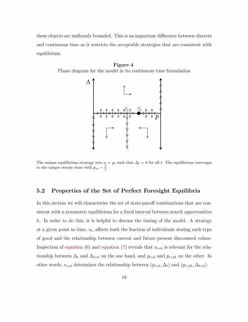
Figure 4Phase diagram for the model in its continuous time formulation

21

32

p2 3

The unique equilibrium strategy sets st = pt such that ∆t = 0 for all t. The equilibrium convergesto the unique steady state with pss = 2

3 .

5.2 Properties of the Set of Perfect Foresight Equilibria

In this section we will characterize the set of state-payoff combinations that are con-

sistent with a symmetric equilibrium for a fixed interval between search opportunities

h. In order to do this, it is helpful to discuss the timing of the model. A strategy

at a given point in time, st, affects both the fraction of individuals storing each type

of good and the relationship between current and future present discounted values.

Inspection of equation (6) and equation (7) reveals that st+h is relevant for the rela-

tionship between ∆t and ∆t+h on the one hand, and pt+h and pt+2h on the other. In

other words, st+h determines the relationship between (pt+h,∆t) and (pt+2h,∆t+h).

18

We now characterize the set of points that are consistent with a symmetric equi-

librium.

Proposition 1 Let pt, st,∆t−ht∈T be a sequence that satisfies equations (5), (6),

and (7). This an equilibrium for an economy with initial condition p0 if and only

if

∆t ∈[∆(pt+h),∆(pt+h)

]where ∆(p) ≡ −β(h)γ(h)p and ∆(p) ≡ β(h)γ(h)(1− p) with γ(h) ≡ α(h)

3u.

Proof. See Appendix E.

Figure 5Phase diagram for the model in its discrete time formulation for step size h

p

21

32

h

p2 3

p

Figure 5, a partial phase diagram for a given interval between search opportunities,

h, gives a graphical representation of the main ideas in the proof of Proposition 1.

Note that on the vertical axis we plot ∆β(h)

. This corresponds to the value at the

beginning of the next time period, so that both pt+h and ∆t

β(h)refer to values at the

beginning of period t+ h.

19

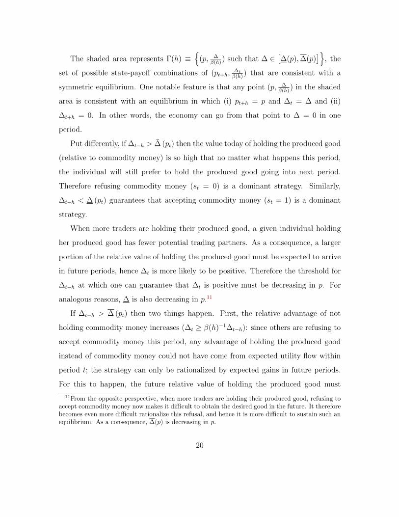
The shaded area represents Γ(h) ≡

(p, ∆β(h)

) such that ∆ ∈[∆(p),∆(p)

], the

set of possible state-payoff combinations of (pt+h,∆t

β(h)) that are consistent with a

symmetric equilibrium. One notable feature is that any point (p, ∆β(h)

) in the shaded

area is consistent with an equilibrium in which (i) pt+h = p and ∆t = ∆ and (ii)

∆t+h = 0. In other words, the economy can go from that point to ∆ = 0 in one

period.

Put differently, if ∆t−h > ∆ (pt) then the value today of holding the produced good

(relative to commodity money) is so high that no matter what happens this period,

the individual will still prefer to hold the produced good going into next period.

Therefore refusing commodity money (st = 0) is a dominant strategy. Similarly,

∆t−h < ∆ (pt) guarantees that accepting commodity money (st = 1) is a dominant

strategy.

When more traders are holding their produced good, a given individual holding

her produced good has fewer potential trading partners. As a consequence, a larger

portion of the relative value of holding the produced good must be expected to arrive

in future periods, hence ∆t is more likely to be positive. Therefore the threshold for

∆t−h at which one can guarantee that ∆t is positive must be decreasing in p. For

analogous reasons, ∆ is also decreasing in p.11

If ∆t−h > ∆ (pt) then two things happen. First, the relative advantage of not

holding commodity money increases (∆t ≥ β(h)−1∆t−h): since others are refusing to

accept commodity money this period, any advantage of holding the produced good

instead of commodity money could not have come from expected utility flow within

period t; the strategy can only be rationalized by expected gains in future periods.

For this to happen, the future relative value of holding the produced good must

11From the opposite perspective, when more traders are holding their produced good, refusing toaccept commodity money now makes it difficult to obtain the desired good in the future. It thereforebecomes even more difficult rationalize this refusal, and hence it is more difficult to sustain such anequilibrium. As a consequence, ∆(p) is decreasing in p.

20

increase by at least the discount rate. Second, the fraction of individuals holding

commodity money falls (pt+h > pt). This means that next period there will be

even fewer potential trading partners for those without commodity money, making

it even harder to get utility flows next period. As a consequence, we can guarantee

∆t > ∆ (pt+h).12 The same reasoning holds in each future period, so that ∆t grows

exponentially and eventually violates the uniform bound implied by Lemma 1. Such

a path is not consistent with equilibrium because this unboundedly large future value

never arrives.

When ∆t−h < ∆ (pt), the analysis is similar, with one slight complication. Here the

relative value of commodity money is so high that no matter what happens accepting

commodity money (st = 1) is the dominant strategy. By an identical argument one

can show that ∆t ≤ β(h)−1∆t−h: since others will be accepting commodity money, the

value of already having commodity money is low this period, and this must be made

up in future periods. The change in the fraction of people holding commodity money

is trickier. Among those holding commodity money, some will be able to trade their

commodity money for their desired good, so there is a natural force increasing the

fraction not holding commodity money (p). If every trader is accepting commodity

money, then the fraction holding their produced good would fall when p > 12

and rise

when p < 12. If p is falling, then by the same reasoning as above, we can guarantee

that ∆t < ∆ (pt+h). When p is rising, commodity money is more likely to deliver the

desired good next period, so one might think it is possible that even with the increased

relative value of commodity money (|∆t|) that the relative value the following period

(∆t+h) need not be negative. However we can show algebraically that the increase in

magnitude of ∆ is large enough to dominate the rise in p, and hence we can guarantee

12This can be seen graphically. If s = 0 is played, then the changes in ∆ and p are both positive,which means that the next point in the sequence is also above ∆(p) (this can be seen from the slopeof ∆(p)).

21

that ∆t < ∆ (pt+h) in this case as well. In either case, |∆t| grows exponentially

and eventually violates the uniform bound.

5.3 Frequency of Search and the Set of Perfect Foresight

Equilibria

The height of set of points consistent with symmetric equilibrium Γ(h) is given by

γ(h) = α(h)3u. As h decreases, the area of this set shrinks in proportion to α(h).

In the limit, α(h), and hence γ(h), approaches zero. In this case Figure 5 coincides

exactly with the phase diagram of the continuous search model depicted in Figure 4.

The only surviving equilibrium is the Zero Equilibrium.

The set of possible equilibrium payoffs is increasing with α(h) as individuals are

more likely to find a trading partner each period. This means that a larger fraction of

the payoff comes from expected utility from a single search, and less from future flows.

As a consequence the set of future payoffs consistent with an initial value of ∆t−h is

larger, and in particular it is less likely that the sign of ∆t, and hence the strategy

st, is pinned down. The set of points in the state-payoff space Γ(h) are precisely the

combinations for which the sign of ∆h is not pinned down.

We can also derive some properties of the sequence of inventories and trading

strategies that are consistent with equilibrium. We show that for any equilibrium,

the sequence of inventories is “close” to that of the Zero Equilibrium. More formally,

the set of sequences of inventories that are consistent with equilibrium converges

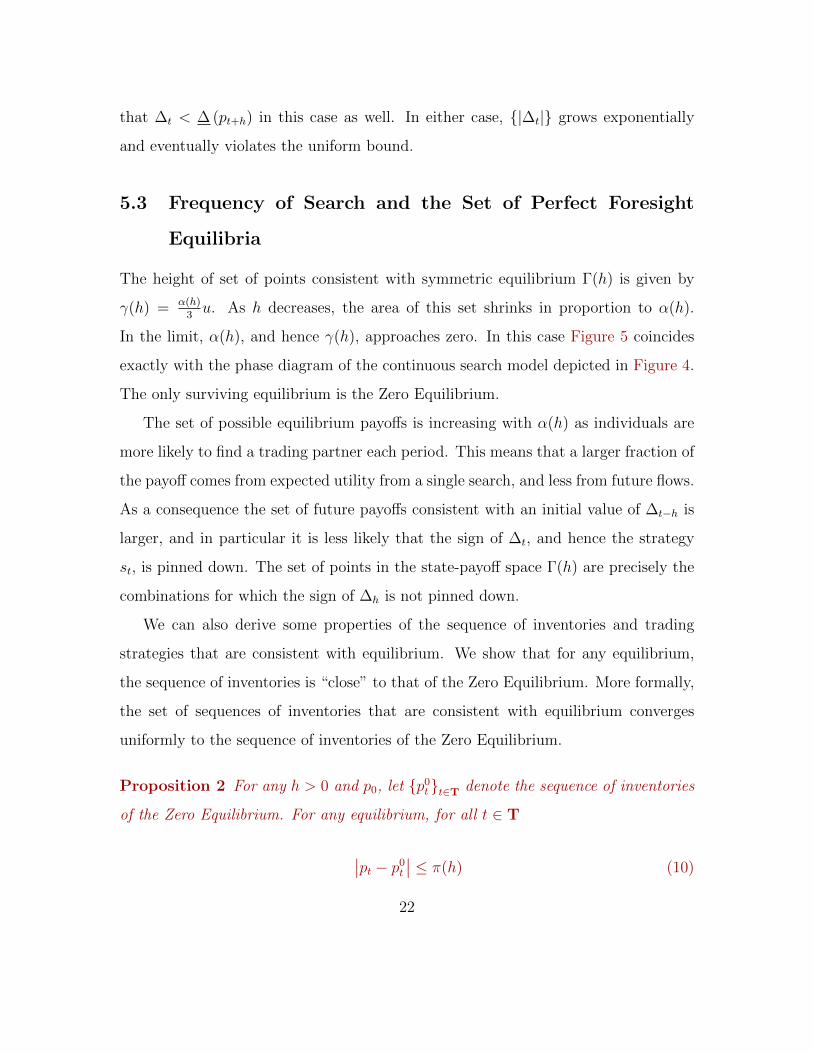
uniformly to the sequence of inventories of the Zero Equilibrium.

Proposition 2 For any h > 0 and p0, let p0tt∈T denote the sequence of inventories

of the Zero Equilibrium. For any equilibrium, for all t ∈ T

∣∣pt − p0t

∣∣ ≤ π(h) (10)

22

where limh→0 π(h) = 0.

Proof. See Appendix D.1.

This proposition follows from the fact that both ∆t and ∆t+Nh must be within

bounds that shrink as search becomes more frequent and h falls. Given ∆t, this puts

a restriction on the strategies that can be played between periods t and t + Nh. As

the bounds on ∆ shrink, the evolution of p implied by those strategies within those

N periods is increasingly constricted and converges to that of the Zero Equilibrium.

To get further insight into this restriction on strategies, we can also show that

the strategies played will also be ”close” to those of the Zero Equilibrium. The next

proposition shows that as search becomes more frequent, the local average of the

trading strategies converges to the strategies of the Zero Equilibrium.

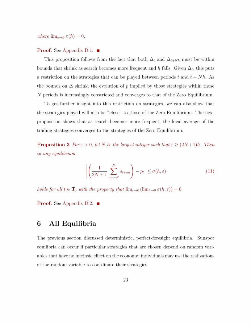
Proposition 3 For ε > 0, let N be the largest integer such that ε ≥ (2N+1)h. Then

in any equilibrium, ∣∣∣∣∣(

1

2N + 1

N∑n=−N

st+nh

)− pt

∣∣∣∣∣ ≤ σ(h, ε) (11)

holds for all t ∈ T, with the property that limε→0 (limh→0 σ(h, ε)) = 0

Proof. See Appendix D.2.

6 All Equilibria

The previous section discussed deterministic, perfect-foresight equilibria. Sunspot

equilibria can occur if particular strategies that are chosen depend on random vari-

ables that have no intrinsic effect on the economy; individuals may use the realizations

of the random variable to coordinate their strategies.

23

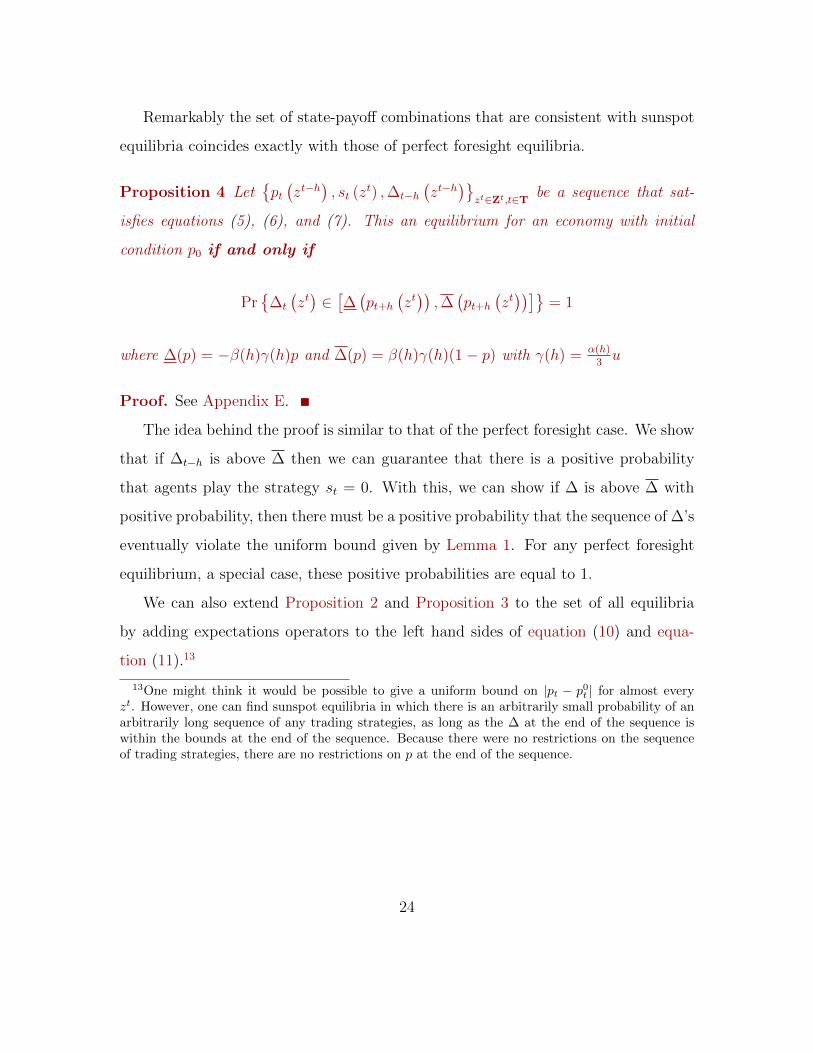
Remarkably the set of state-payoff combinations that are consistent with sunspot

equilibria coincides exactly with those of perfect foresight equilibria.

Proposition 4 Letpt(zt−h

), st (zt) ,∆t−h

(zt−h

)zt∈Zt,t∈T be a sequence that sat-

isfies equations (5), (6), and (7). This an equilibrium for an economy with initial

condition p0 if and only if

Pr

∆t

(zt)∈[∆(pt+h

(zt)),∆(pt+h

(zt))]

= 1

where ∆(p) = −β(h)γ(h)p and ∆(p) = β(h)γ(h)(1− p) with γ(h) = α(h)3u

Proof. See Appendix E.

The idea behind the proof is similar to that of the perfect foresight case. We show

that if ∆t−h is above ∆ then we can guarantee that there is a positive probability

that agents play the strategy st = 0. With this, we can show if ∆ is above ∆ with

positive probability, then there must be a positive probability that the sequence of ∆’s

eventually violate the uniform bound given by Lemma 1. For any perfect foresight

equilibrium, a special case, these positive probabilities are equal to 1.

We can also extend Proposition 2 and Proposition 3 to the set of all equilibria

by adding expectations operators to the left hand sides of equation (10) and equa-

tion (11).13

13One might think it would be possible to give a uniform bound on |pt − p0t | for almost everyzt. However, one can find sunspot equilibria in which there is an arbitrarily small probability of anarbitrarily long sequence of any trading strategies, as long as the ∆ at the end of the sequence iswithin the bounds at the end of the sequence. Because there were no restrictions on the sequenceof trading strategies, there are no restrictions on p at the end of the sequence.

24

7 Conclusion

The literature following Kiyotaki and Wright (1989) has studied economies with ex-

plicit search frictions to learn how these frictions affect economic behavior. We study

how a feature of the environment, the frequency of search, interacts with these search

frictions to shape potential equilibrium outcomes. In particular, we shed light on eco-

nomic forces in the model that can generate multiplicity, and show how these change

as search becomes more frequent.

We show that as search frequency increases, the set of dynamic equilibria shrinks

uniformly in three dimensions: (i) equilibrium payoffs associated a given state of

the economy; (ii) the average strategy played over any given unit of time; and (iii)

dynamic paths of the state variables.

To do this, we focus on symmetric equilibria in a symmetric environment. This

restriction allows us to cleanly characterize several dimensions of the set of dynamic

equilibria. While symmetric equilibria are often the object of interest14 a natural

question is how our results generalize to asymmetric equilibria or environments. In

these more general environments characterizing the set of equilibria is considerably

more difficult technically. While there may not be a unique dynamic equilibrium, we

conjecture that the set dynamic equilibria shrinks uniformly as agents search more

frequently (indexed by the characteristics we describe above). We further conjecture

that when search is frequent every equilibrium can be approximated by an element

of the set of continuous search equilibria. In other words, when search is frequent,

much of the multiplicity will not matter.

14See Kiyotaki and Wright (1993) for an early example.

25

References

Abreu, D., P. Milgrom, and D. Pearce (1991): “Information and Timing inRepeated Partnerships,” Econometrica, 59(6), 1713–33.

Aiyagari, S. R., and N. Wallace (1992): “Fiat Money in the Kiyotaki-WrightModel,” Economic Theory, 2(4), 447–464.

Benhabib, J., and R. E. Farmer (1999): “Indeterminacy and sunspots in macroe-conomics,” in Handbook of Macroeconomics, ed. by J. B. Taylor, and M. Woodford,vol. 1 of Handbook of Macroeconomics, chap. 6, pp. 387–448. Elsevier.

Boldrin, M., and L. Montrucchio (1986): “On the indeterminacy of capitalaccumulation paths,” Journal of Economic Theory, 40(1), 26–39.

Carlstrom, C. T., and T. S. Fuerst (2001): “Timing and real indeterminacyin monetary models,” Journal of Monetary Economics, 47(2), 285–298.

Fudenberg, D., and D. K. Levine (2009): “Repeated Games with FrequentSignals-super-,” The Quarterly Journal of Economics, 124(1), 233–265.

Hintermaier, T. (2005): “A sunspot paradox,” Economics Letters, 87(2), 285–290.

Jovanovic, B., and R. W. Rosenthal (1988): “Anonymous sequential games,”Journal of Mathematical Economics, 17(1), 77–87.

Kehoe, T., N. Kiyotaki, and R. Wright (1993): “More on Money as a Mediumof Exchange,” Economic Theory, 3.

Kiyotaki, N., and R. Wright (1989): “On Money as a Medium of Exchange,”Journal of Political Economy, 97(4), 927–54.

(1993): “A Search-Theoretic Approach to Monetary Economics,” AmericanEconomic Review, 83(1), 63–77.

Appendix

A Proof of Lemma 1

We first show that for any equilibrium that satisfies the conditions of Definition 1,∆t (zt)zt∈Zt,t∈T has a uniform bound with probability 1. It is straightforward to

26

show that value functions V i,jt (zt) can be bounded above and below by bounds that

are independent of zt and t. For the upper bound, we can assume that the individualis able to consume at every chance meeting. For the lower bound we can assume thatthe individual never consumes. The value function V i,j

t (zt) can therefore be bounded

by 0 ≤ V i,jt (zt) ≤ α(h)u

1−β(h). It follows that ∆t(z

t) is bounded above and below by

bounds that are independent of zt and t. The other conditions of Definition 1 aretrivially satisfied.

Second, we show that if a sequence pt, st,∆t−ht∈T (i) satisfies equation (5),equation (6), and equation (7) and (ii) ∆t(z

t)zt∈Zt,t∈T is uniformly bounded, then wecan construct a sequence of pt, st, V i,i+1

t−h , V i,i+2t−h t∈T that is a symmetric equilibrium.

We need to show that one can construct a sequence of value functions that satisfythe symmetric versions of equation (3), equation (4), and transversality.

For a given sequence, define M1t (zt) and M2

t (zt) to be

M1t (zt) = β(h)

α(h)

3[pt(z

t−h)(−∆t(zt)) + (1− pt(zt−h))u+ pt(z

t−h)st(zt)u]

and

M2t (zt) = β(h)α(h)

3

[(1− pt(zt−h)

)(1− st(zt)) (u+ ∆t(z

t))+pt(z

t−h) (u+ ∆t(zt)) +

(1− pt(zt−h)

)(1− st(zt)) (∆t(z

t))]

Iterating equation (3) and equation (4), and taking the limit as N →∞ gives

V i,i+1−h (z−h) = E−h [

∑∞n=0 β(h)nM1

nh] + limN→∞ E−h[β(h)N+1V i,i+1

Nh

]V i,i+2−h (z−h) = E−h [

∑∞n=0 β(h)nM2

nh] + limN→∞ E−h[β(h)N+1V i,i+2

Nh

]where Et (·) = E (· | zt). The fact that ∆t(z

t) is uniformly bounded implies thatthe terms E−h

[∑∞n=0 β(h)nM1

nh(znh)]

and E−h[∑∞

n=0 β(h)nM2nh(z

nh)]

are finite. If

we set V i,i+10 (z0) = −E−h

[∑∞n=0 β(h)nM1

nh(znh)], then transversality must be sat-

isfied. Since equation (3) and equation (4) are satisfied by construction, this is anequilibrium.

B Two Period Cycles

In this section we show that in a neighborhood around h = 0, we can always constructa two period cycle: in even periods the economy is at ∆e, pe, se, and in odd periodsat ∆o, po, so. We can evaluate equation (5), equation (6), and equation (7) atthe values of odd and even periods to obtain a system of four unknowns and tworestrictions. We will look for cycles in which so = 1 and ∆e = 0, so the four equations

27

become,

0 = ∆o + α(h)3u[1− po]− α(h)

32po∆o

∆o = β(h)α(h)3u[se − pe]

po = pe − α(h)3p2ese + α(h)

3(1− pe)[2(1− pe)(1− se) + pe]

pe = po − α(h)3p2o + α(h)

3(1− po)po

These four equations will then determine the values of the unknowns, se, ∆o, po,and pe. To verify that such cycle exists, we must show that (i) ∆o ≤ 0 (so that so = 1is optimal), and (ii) that se ∈ [0, 1] (so that the cycle is feasible).

The first equation implies that ∆o ≤ 0, and with this the second equation impliesthat se ≤ pe ≤ 1. We must now verify that se ≥ 0. We can eliminate ∆0 and reducethe system to the following three equations

se = S(po) ≡ po

[1− α(h)

3po + α(h)

3(1− po)

]− 1−po

[1−α(h)32po]β(h)

pe = P (po) ≡ po − α(h)3p2o + α(h)

3(1− po)po

0 = g(po) ≡ P (po)− α(h)3P (po)

2S(po)− po+α(h)

3(1− P (po)) [2 (1− P (po)) (1− S(po)) + P (po)]

The third equation defines candidate values of po consistent with the specified cycle,while the functions S and P give the corresponding values of se and pe respectively.We can show that se is strictly increasing in po,

S ′(po) = 1− α(h)po +α(h)

3(1− po) +

1− 2α(h)3[

1− α(h)3

2po

]2

β(h)> 0

Let po solve S(po) = 0. The inventory level po is useful as it provides a lowerbound for the required level of po for a cycle to exist. There is a unique po ∈

(12, 1),

since S(1) = 1− α(h)3∈ (0, 1), S(1

2) = 1

2

[1− 1

[1−α(h)3 ]β(h)

]< 0, and S ′(p) > 0.

Because S is strictly increasing, if we can find a po ∈ [po, 1) that satisfies g(po) = 0then we can guarantee that se ∈ [0, 1].

We show first that g(1) < 0 (using P (1) = S(1)):(α(h)

3

)−1

g(1) = −α(h)3− P (1)3 + 2[1− P (1)]3 − P (1)2

= −3P (1)3 + 5P (1)2 − 6P (1)− α(h)3

+ 2

= α(h)9

(α(h)2 − 4α(h) + 12)− 2

28

which is negative for any α(h) ∈ (0, 1]. We next show that in a neighborhood aroundh = 0, g(po) > 0. By the mean value theorem, this will guarantee that there is asolution po ∈ [po, 1), and consequently the existence of a two point cycle.

We can use the definition of P along with the fact that po ≥ po >12

to get

P (po)− po =α(h)

3po(1− 2po)

and therefore P (po) < po. Now we turn to evaluate g(po),

g(po) = P (po)− po +α(h)

3[1− P (po)][2− P (po)]

This can be reduced to(α(h)

3

)−1

g(po) = [1− P (po)] [2− P (po)]− po (2po − 1)

We can construct a lower bound for this object. Noting that po > P (po),(α(h)

3

)−1

g(po) > −(p2o + 2po − 2

)If po ∈

(12,√

(3)− 1)

then we can guarantee that g(p0) > 0, and that there is a

cycle. Now, from the definition of S, we can see that limh→0po = 12, so along with

the continuity of S, this implies that in a neighborhood around h = 0 this conditionwill be satisfied.

C Proof of Proposition 1

We develop the proof as a sequence of claims. Let pt, st,∆t−ht∈T be a sequencethat satisfies equation (5), equation (6), and equation (7).

Claim 1 If ∆t > ∆(pt+h) then ∆t+h > ∆(pt+2h) and ∆t+h ≥ ∆t/β(h). Similarly, if∆t < ∆(pt+h) then ∆t+h < ∆(pt+2h) and ∆t+h ≤ ∆t/β(h).

Proof. Rearranging the perfect foresight version of equation (7) gives

∆t+h =∆t − β(h)α(h)

3u(st+h − pt+h)

β(h)Ωt+h

29

where Ωt = 1 − α(h)3

[ptst + 2(1− pt)(1− st) + pt] ∈ (0, 1]. ∆t > ∆(pt+h) guaranteesthat ∆t+h > 0 and hence st+h = 0. Similarly, ∆t < ∆(pt+h) guarantees that ∆t+h < 0and hence st+h = 1.

Another rearrangement of equation (7) gives

β(h)∆t+h −∆t = −β(h)α(h)

3u(st+h − pt+h) + β(h)(1− Ωt+h)∆t+h

If ∆t+h > 0, then st+h = 0 and hence β(h)∆t+h ≥ ∆t. Similarly, if ∆t+h < 0, thenst+h = 1 and hence β(h)∆t+h ≤ ∆t.

We can also rearrange equation (6) to be

pt+2h − pt+h =α(h)

3pt+h(1− 2pt+h)st+h + (2− pt+h)(1− pt+h)(1− st+h)

If st+h = 0 then pt+2h ≥ pt+h. If st+h = 1 then the sign of pt+2h − pt+h depends onwhether pt+h ≷ 1/2.

Consider first the case of ∆t > ∆(pt+h). We have shown that ∆t+h ≥ ∆t andthat pt+2h ≥ pt+h. These, along with the fact that ∆ is decreasing in p imply that∆t+h > ∆(pt+2h).

Now consider ∆t < ∆(pt+h). We have shown that ∆t+h ≤ ∆t. If in additionpt+h ≥ 1/2, then pt+2h ≤ pt+h. These along with the fact that ∆ is decreasing in pimply that ∆t+h < ∆(pt+2h).

If, however, pt+h < 1/2 then we cannot rely on this argument because pt+2h > pt+h.Instead we check algebraically that ∆t+h < ∆(pt+2h). We can write

∆t+h −∆t

pt+2h − pt+h=

(1− β(h))∆t+h − β(h)[α(h)

3u(1− pt+h)− α(h)

32pt+h∆t+h

]α(h)

3pt+h(1− 2pt+h)

< −β(h)u(1− pt+h)pt+h(1− 2pt+h)

< −β(h)uα(h)

3= −β(h)γ(h)

where the last inequality follows as pt+h <12

and α(h)3< 1.

Starting with ∆t < −β(h)γ(h)pt+h, we have that

∆t+h < −β(h)γ(h)pt+2h + β(h)γ(h)pt+h + ∆t

< −β(h)γ(h)pt+2h

< ∆(pt+2h)

30

which completes the proof

Claim 2 Let pt, st,∆t−ht∈T be a sequence that satisfies equations (5), (6), and(7). This an equilibrium for an economy with initial condition p0 if and only if∆t ∈

[∆(pt+h),∆(pt+h)

].

Proof. If ∆t 6∈[∆(pt+h),∆(pt+h)

]for some t, then the previous claim implies

that ∆t+Nh 6∈[∆(pt+(N+1)h),∆(pt+(N+1)h)

]for all N > 0. Therefore |∆t+Nh| ≥

β(h)−N |∆t|. This would violate the uniform bound on ∆t, so the sequence cannotbe an equilibrium.

If, however, ∆t ∈[∆(pt+h),∆(pt+h)

]for all t ∈ T then the sequence ∆t has a

uniform bound. By Lemma 1, the sequence is consistent with equilibrium.

D Proofs of Proposition 2 and Proposition 3

We first prove a preliminary result that will help us prove Proposition 2 and Propo-sition 3. Let pt, st,∆t−ht∈T be an sequence consistent with equilibrium.

Lemma 2 For any N > 0, the following inequality holds:

N∑n=1

ωt,n,N (st+nh − pt+nh) ≤ 21− β(h) (1− α(h))

1− [β(h) (1− α(h))]N

where

ωt,n,N =

∏n−1j=1 ρt+jh∑N

n=1

(∏n−1j=1 ρt+jh

)and ρt = β(h)

(1− α(h)

3[pt (1 + st) + 2 (1− pt) (1− st)]

).

Proof. Under perfect foresight equation (7) can be written as

∆t = β(h)α(h)

3u (st+h − pt+h) + ρt+h∆t+h

We can iterate this equation to get

∆t = β(h)α(h)

3u

N∑n=1

(n−1∏j=1

ρt+jh

)(st+nh − pt+nh) +

(N∏n=1

ρt+nh

)∆t+Nh

where∏0

j=1 is defined to be 1.

31

Reordering terms, dividing by∑N

n=1

(∏n−1j=1 ρt+jh

), and using the definition of

ωt,n,N provides

β(h)α(h)

3u

N∑n=1

ωt,n,N (st+nh − pt+nh) =∆t −

(∏Nn=1 ρt+nh

)∆t+Nh∑N

n=1

(∏n−1j=1 ρt+jh

)Since ρt ∈

(β(h)

(1− 2

3α(h)

), β(h)

], we can bound the right hand side of this equa-

tion. The denominator is greater than∑N

n=1

[β(h)(1− 2

3α(h))

]n−1, while the magni-

tude of the numerator is less than 2β(h)γ(h). These give the following bound:

N∑n=1

ωt,n,N (st+nh − pt+nh) ≤ 21− β(h)

(1− 2

3α(h)

)1−

[β(h)

(1− 2

3α(h)

)]N (12)

We can also use the bounds on ρ to bound each individual ω

ωt,n,N ∈

([1− 2

3α(h)

]NN

,1

N[1− 2

3α(h)

]N)

(13)

which completes the proof.

D.1 Proof of Proposition 2

In any equilibrium, the sequence of inventories follows the equation

pt+h = pt +α(h)

3

[−p2

t st + 2(1− pt)2(1− st) + pt(1− pt)]

Similarly, the sequence of inventories for the Zero Equilibrium must also follow thelaw of motion. Combining these equations give

pt+h − p0t+h = Φt(st − pt)− λt(pt − p0

t )

where Φt and λt are defined and bounded as follows

Φt = 1− α(h)3− [3(pt + p0

t )− 4] p0t − 3 + (pt + p0

t ) + p2t + 2(1− pt)2

∈[1− 5

3α(h), 1− 2

3α(h)

] (14)

and

λt =α(h)

3

[p2t + 2(1− pt)2

]∈[

2

9α(h),

2

3α(h)

](15)

32

We can iterate this equation over N periods to get

pt+Nh−p0t+Nh =

N−1∑n=0

(N−1∏j=n+1

Φt+jh

)λt+nh(st+nh−pt+nh)+

(N−1∏n=0

Φt+nh

)(pt−p0

t ) (16)

where again the product∏N−1

n=N is defined to be one.We now provide a bound on the divergence of inventories from those of the Zero

Equilibrium among the first N periods. Since p0 = p00 and |st − pt| ≤ 1 we can

use equation (16) and the upper bounds on Φ and λ given by equation (14) andequation (15) to get:

∣∣pNh − p0Nh

∣∣ ≤ 2

3α(h)

N−1∑n=0

(1− 2

3α(h)

)n= 1−

[1− 2

3α(h)

]NDefine π0(h,N) ≡ 1−

[1− 2

3α(h)

]Nto be this bound.

We next provide a bound on the subsequent divergence of inventories from thoseof the Zero Equilibrium. We can write equation (16) as

pt+Nh − p0t+Nh =

(1−

∏N−1n=0 Φt+nh

)χt,N

∑N−1n=0

λt+nhλt

φt,n,N(st+nh − pt+nh)

+(∏N−1

n=0 Φt+nh

)(pt − p0

t )(17)

where χ and φ are defined by

χt,N = λt

∑N−1n=0

(∏N−1j=n+1 Φt+jh

)1−

∏N−1n=0 Φt+nh

φt,n,N =

∏N−1j=n+1 Φt+jh∑N−1

n=0

(∏N−1j=n+1 Φt+jh

)We will show that the term χt,N

∑N−1n=0

λt+nhλt

φt,n,N(st+nh − pt+nh) can be boundedby a function π1(h,N). This is useful because equation (17) would then imply thatif |pt − p0

t | ≤ ε for some ε ≥ π1(N, h), then we also have∣∣pt+Nh − p0

t+Nh

∣∣ ≤ ε.To do this, we first show that |χt,N | ≤ 1. Since χ is increasing in each Φt, we can

use the upper bounds on λ and Φ to get

|χt,N | ≤

∣∣∣∣∣23α(h)

∑N−1n=0

(1− 2

3α(h)

)n1−

(1− 2

3α(h)

)N∣∣∣∣∣ = 1

33

Next we can bound∑N−1

n=0λt+nhλt

φt,n,N(st+nh − pt+nh) by decomposing it into threeparts using

λt+nhλt

φt,n,N =

(λt+nh − λt

λtφt+nh

)+ (φt,n,N − ωt,n,N) + (ωt,n,N)

Using |st − pt| ≤ 1 and φt,n,N > 0 gives

∣∣∣∣∣N−1∑n=0

λt+nhλt

φt,n,N(st+nh − pt+nh)

∣∣∣∣∣ ≤N−1∑n=0

∣∣∣∣λt+nh − λtλt

∣∣∣∣φt,n,N +N−1∑n=0

|φt,n,N − ωt,n,N)|

+

∣∣∣∣∣N−1∑n=0

ωt,n,N(st+nh − pt+nh)

∣∣∣∣∣We will bound each of these three terms separately. First, note that equation (6)

implies

|pt+h − pt| =α(h)

3|(1− 2pt) ptst + (2− pt) (1− pt) (1− st)| ≤

2

3α(h)

and hence |pt+nh − pt| ≤ n(

23α(h)

). We can also use the definition of λ to write∣∣∣∣λt+nh − λtλt

∣∣∣∣ =

∣∣∣∣∣ α(h)3

(pt+nh − pt) (3(pt+nh + pt)− 4)

λt

∣∣∣∣∣ ≤α(h)

3

(n2

3α)

429α(h)

≤ 4Nα(h)

Since∑N−1

n=0 φt,n,N = 1, we have∣∣∣∣∣N−1∑n=0

∣∣∣∣λt+nh − λtλt

∣∣∣∣φt,n,N∣∣∣∣∣ ≤ 4Nα(h)

We can use the bound on Φ given by equation (14) to get upper and lower boundsfor φ:

φt,n,N ∈

(1

N

(1− 5

3α(h)

1− 23α(h)

)N,

1

N

(1− 2

3α(h)

1− 53α(h)

)N)

34

This, in combination with the bounds on ω from equation (13) imply that

|φt,n,N − ωt,n,N | ≤ 1N

maxι∈−1,1

∣∣∣∣(1− 23α(h)

)ιN − (1− 23α(h)

1− 53α(h)

)ιN ∣∣∣∣=

(1− 2

3α(h)

)N [(1− 5

3α(h)

)−N − 1]

Lastly, the third term can be bounded using Lemma 2. In total, these give theresult that

χt,N

N−1∑n=0

λt+nhλt

φt,n,N(st+nh − pt+nh) ≤ π1(h,N)

with

π1(h,N) ≡ 4Nα(h) +(1− 2

3α(h)

)N ((1− 5

3α(h)

)−N − 1)

+ 21−β(h)(1− 2

3α(h))

1−[β(h)(1− 23α(h))]

N

At this point we have shown that for any N , inventories in the first N periodsare within π0(h,N) of those of the Zero Equilibrium. We have also shown that ifinventories in the first N periods are within ε of those of Zero Equilibrium for anyquantity ε ≥ π1(h,N), then inventories in all subsequent periods are as well. We cancombine these two statements to arrive at a uniform bound for the entire sequence.Define π(h,N) = maxπ0(h,N), π1(h,N). We therefore have that for any N > 0and any t ∈ T, inventories are within π(N, h) of those of the Zero Equilibrium:∣∣pt − p0

t

∣∣ ≤ π(h,N)

Let π(h) = minN π(h,N). This will be a bound for |pt − p0t |.

Lastly, we can show that limh→0 π(h) = 0. Let ν(h) = h−1/2. From the definitionsof π0 and π1 it is straightforward to show that limh→0 π0(h, ν(h)) = limh→0 π1(h, ν(h)) =0. Since π(h) ≤ π(h, ν(h)), these imply that limh→0 π(h) = 0.

D.2 Proof of Proposition 3

In a similar way, we can show that, at least locally, the average trading strategyplayed coincides with that of the Zero Equilibrium.

For ε > 0, let N be the largest integer such that ε ≥ (2N + 1)h. We can form abound on the local average trading strategy:

35

∣∣∣( 12N+1

∑Nn=−N st+nh

)− pt

∣∣∣ ≤ ∣∣∣∑Nn=−N

(1

2N+1 − ωt−N,n+N,2N+1

)(st+nh − pt+nh)

∣∣∣+∣∣∣∑N

n=−N ωt−N,n+N,2N+1 (st+nh − pt+nh)∣∣∣

+∣∣∣ 12N+1

∑Nn=−N (pt+nh − pt)

∣∣∣The first sum can be bounded using the bound on ω given by equation (13)

∣∣∣∑Nn=−N

(1

2N+1 − ωt−N,n+N,2N+1

)(st+nh − pt+nh)

∣∣∣ ≤ ∑Nn=−N

∣∣∣ 12N+1 − ωt−N,n+N,2N+1

∣∣∣≤

(1− 2

3α(h))−(2N+1) − 1

The second summation can be bounded using equation (12). The third term can bebounded using the fact that |pt+h − pt| ≤ α(h), which can be seen from equation (6).This implies that ∣∣∣∣∣ 1

2N + 1

N∑n=−N

(pt+nh − pt)

∣∣∣∣∣ ≤ Nα(h)

We can combine these to form a single bound for a fixed ε:

σ(ε, h) =

(1− 2

3α(h)

)−ε/h− 1 + 2

1− β(h)(1− 2

3α(h)

)1−

[β(h)

(1− 2

3α(h)

)]ε/h +ε

2α(h)

For a fixed ε, each of these three bounds goes to a finite number as h→ 0:

limh→0

σ(ε, h) = e23α0ε − 1 +

ε

2α0

It follows that limε→0 (limh→0 σ(ε, h)) = 0.

E Proof of Proposition 4

We develop the proof as a sequence of claims. For ease of exposition we drop theargument z from pt, st, and ∆t.

Let pt, st,∆t−hzt∈Zt,t∈T be a sequence that satisfies equation (5), equation (6),and equation (7). Also, Let Gt,n be the event that ∆t−jh 6∈ [∆(pt−(j−1)h),∆(pt−(j−1)h)]for all j ∈ (0, ..., n). We can make the following claims about the sequence:

Claim 3 If Pr (Gt,n) > 0 then Pr(Gt+h,n+1 and |∆t+h| ≥ |∆t|

β(h)

)> 0

36

Proof. The following definitions will assist in the exposition of the proof. As be-fore, let Ωt = α(h)

3[ptst + 2(1− pt)(1− st) + pt]. Note that Ωt ∈ [0, 1]. Also let

Xt+h = −∆t + β(h)∆t+h + β(h)α(h)3

(st+h − pt+h)u − β(h)Ωt+h∆t+h. equation (7)can be rewritten as 0 = Et [Xt+h], where Et(·) = E(· | zt). This implies both thatPr (Xt+h ≥ 0|zt) > 0 and also that Pr (Xt+h ≤ 0|zt) > 0 for all zt. We therefore havethat if Pr (Gt,n) > 0 then either Pr

(Gt,n and ∆t > ∆(pt+h) and Xt+h ≥ 0

)> 0 or

Pr (Gt,n and ∆t < ∆(pt+h) and Xt+h ≤ 0) > 0. We will show that in either case

Pr

(Gt+h,n+1 and |∆t+h| ≥

|∆t|β(h)

)> 0

.First, consider the event in which ∆t > ∆(pt+h). If ∆t+h ≤ 0, then it must be

that Xt+h < 0, because ∆t > ∆(pt+h) ≥ β(h)α(h)3

(st+h − pt+h)u. Consequently, ifXt+h ≥ 0, then ∆t+h > 0 and therefore st+h = 0. The combination of Xt+h ≥ 0and st+h = 0 imply that ∆t+h ≥ ∆t

β(h)and pt+2h > pt+h. Since ∆(p) is decreasing in

p, these also imply that ∆t+h > ∆(pt+2h). We therefore have that in the event that

∆t > ∆(pt+h) and Xt+h ≥ 0, then ∆t+h 6∈ [∆(pt+2h),∆(pt+2h)] and |∆t+h| ≥ |∆t|β(h)

.

Now we turn to the event in which ∆t < ∆(pt+h), Xt+h ≤ 0, and ∆t+h < 0. Wewill show that in this case ∆t+h < ∆(pt+2h). This is more difficult because the changein p is not a monotonic function of p. If ∆t < ∆(pt+h) then in a similar manner asabove we can show that ∆t+h < 0 and st+h = 1. This means that we can write

∆t ≥ β(h)

[∆t+h +

α(h)

3u(1− pt+h)− Ωt+h∆t+h

]and

pt+h = pt +α(h)

3pt(1− 2pt)

We take two cases separately. For each we will show that if ∆t is below the bound,than ∆t+h is below the bound as well. (i) If pt+h ≥ 1

2, then we can show this in a

similar manner as above. Since pt+2h ≤ pt+h and ∆t+h < ∆t < 0, the fact that ∆(p)

37

is decreasing in p implies that ∆t+h < ∆(pt+2h). (ii) If pt+h < 1/2 then we can write

∆t+h −∆t

pt+2h − pt+h≤

(1− β(h))∆t+h − β(h)[α(h)

3u(1− pt+h)− Ωt+h∆t+h

]α(h)

3pt+h(1− 2pt+h)

< −β(h)u(1− pt+h)pt+h(1− 2pt+h)

< −β(h)uα(h)

3= −β(h)γ(h)

where the last inequality follows because pt+h < 12

and α(h)3

< 1. We start with∆t < −β(h)γ(h)pt+h. We then have that

∆t+h < −β(h)γ(h)pt+2h + β(h)γ(h)pt+h + ∆t

< −β(h)γ(h)pt+2h

< ∆(pt+2h)

For both cases we also know that Xt+h ≤ 0. This, in combination with st+h = 1,implies that ∆t+h ≤ ∆t

β(h).

If ∆t+h ≥ 0 then we know that Xt+h > 0 because ∆t < ∆(pt+h) ≤ β(h)α(h)3

(st+h−pt+h)u. This implies that if Xt+h ≤ 0, then ∆t+h < 0. We have therefore shown that

if ∆t < ∆(pt+h) and Xt+h ≤ 0, then ∆t+h 6∈ [∆(pt+2h),∆(pt+2h)] and |∆t+h| ≥ |∆t|β(h)

.

Claim 3 shows that if ∆t 6∈[∆(pt+h),∆(pt+h)

], then the following ∆ is outside

the bounds with positive probability and the magnitude grows exponentially.

Claim 4 If Pr(∆t 6∈ [∆(pt+h),∆(pt+h)]

)> 0 then a sequence of inventories, strate-

gies, and value functionspt(zt−h

), st (zt) ,∆t−h

(zt−h

)zt∈Zt,t∈T is not consistent

with equilibrium.

Proof. Let B be the uniform bound implied by Lemma 1. Assume that there exists at0 such that Pr

(∆t0 6∈ [∆(pt0+h),∆(pt0+h)]

)> 0. This implies that there exists ε > 0

such that Pr(∆t0 6∈ [∆(pt0+h),∆(pt0+h)], |∆t0| > ε

)> 0. Iterating Claim 3 gives the

result

Pr

(∆t0+nh 6∈ [∆(pt0+(n+1)h),∆(pt0+(n+1)h)], |∆t0+nh| ≥

|∆t0 |β(h)n

≥ ε

β(h)

)> 0

Since there exists an N > 0 such that εβ(h)N

> B, we have Pr (|∆t+Nh| > B) > 0.

38