erosion performance indicator: methodology … methods... · describes the svm goals and the...

EROSION PERFORMANCE INDICATOR: METHODOLOGY AND SHARED VISION MODEL APPLICATION

Prepared for:

I.J.C. PLAN FORMULATION AND EVALUATION GROUP

Prepared by:

W.F. BAIRD & ASSOCIATES COASTAL ENGINEERS LTD. OAKVILLE, ONTARIO

MARCH 2004

Erosion Performance Indicator:

Methodology and Shared Vision Model Application

Baird & Associates

This report has been prepared for PFEG by:

W.F. BAIRD & ASSOCIATES COASTAL ENGINEERS LTD. 627 LYONS LANE OAKVILLE, ON L6J 5Z7

For further information please contact (Pete Zuzek (905)845-5385 ext. 425 or Rachel Roblin ext. 437)


Methodology and Shared Vision Model Application

Baird & Associates

TABLE OF CONTENTS

1.0 INTRODUCTION ......................................................................................1

1.1 Shared Vision Model Goals .......................................................................................................1 1.2 Predictive Equations for the Erosion Performance Indicator................................................1

2.0 DATA .......................................................................................................4

2.1 Water Level Database...............................................................................................................4 2.2 County Database ........................................................................................................................4 2.3 Township Database ....................................................................................................................4 2.4 Normal Wave Energy Database................................................................................................5 2.5 Reach Database ..........................................................................................................................5 2.6 Parcel Database ..........................................................................................................................5

3.0 METHODOLOGY FOR EROSION P.I.........................................................6

3.1 Site Selection ...............................................................................................................................6 3.1.1 WAVAD Site Selection ...........................................................................................................6 3.1.2 COSMOS Modeling Site Selection.........................................................................................8

3.2 Cohesive Modeling .....................................................................................................................9 3.2.1 Waves ......................................................................................................................................9 3.2.2 Water Levels............................................................................................................................9 3.2.3 Ice..........................................................................................................................................10 3.2.4 COSMOS Calibration...........................................................................................................10 3.2.5 101-year COSMOS ...............................................................................................................10

3.3 Cohesive Equation Development ............................................................................................10 3.4 Sandy Erosion...........................................................................................................................14 3.5 SVM Application ......................................................................................................................14

3.5.1 Cohesive ................................................................................................................................14 3.5.2 Sandy.....................................................................................................................................16

4.0 ECONOMICS..........................................................................................17

4.1 Parcel Classes............................................................................................................................17 4.2 Method I – Future Liability of Shore Protection...................................................................19

4.2.1 Conditions of Use – Developed Parcels ...............................................................................19 4.2.2 Evaluation Methods..............................................................................................................19 4.2.3 Comparison of Plans ............................................................................................................22

4.3 Method II ..................................................................................................................................23

Erosion Performance Indicator: Methodology and Shared Vision

Model Application

Baird & Associates

Table of Contents

4.3.1 Conditions of Use – Undeveloped Parcels ...........................................................................23 4.3.2 Evaluation Methods..............................................................................................................23

5.0 SUMMARY.............................................................................................26

5.1 Required Data...........................................................................................................................26 5.2 Fields and flags for Parcel Database.......................................................................................27

Erosion Performance Indicator: Methodology and Shared Vision

Model Application

Baird & Associates

Table of Contents

1.0 INTRODUCTION

This report outlines the approach used to evaluate long-term sandy erosion and the methods that will be used to develop the erosion prediction equations for cohesive erosion around Lake Ontario. The economic representation of erosion around the lake is also discussed and the procedure for incorporating these results into the Shared Vision Model (SVM) is also described using Niagara County as an example. Section 1.0 briefly describes the SVM goals and the Erosion Performance Indicator (PI) cohesive predictive equations.

1.1 Shared Vision Model Goals

The Shared Vision Model (SVM) is being created to connect all of the research completed by the Technical Working Groups (TWG) to the decisions that the Study Board has to make on new criteria, operating procedures and ultimately a new Regulation Plan. The model will determine how different plans affect the stakeholders and the economics around Lake Ontario, and will gage these results against criteria and performance indicator goals from each TWG. The SVM is transparent and takes an integrated process approach that will help to make informed decisions that are connected to the research.

1.2 Predictive Equations for the Erosion Performance Indicator

A visual summary of the cohesive Erosion Performance Indicator and the various scales of resolution for the calculations in the SVM are provided in Figure 1.1. This Figure was included in the October 22nd 2003 Baird – PFEG meeting minutes. It is a hypothetical diagram that uses the western end of Lake Ontario to illustrate the methods being developed for the SVM.

• Families of Equations (FEq) are being developed currently on a County/Regional Municipality basis. The equations have been grouped into 0.25m incremental water level bins between 3.0m above and 2.0m below chart datum and have the general form:

Recession = (a x ln(E) + b) x AARR

Where: a = constant (slope)

E = Normal Wave Energy (Joules/m2), calculated monthly

b = constant (intercept)

AARR = Historical Average Annual Recession Rate (m/yr)


Methodology and Application into the Shared Vision Model

Baird & Associates

1

More than one Family of Equations may be required for large counties or counties where the wave climate varies considerably. Each FEQ will follow the evaluation procedure and integration methods presented for Niagara County.

• Normal monthly wave energy will be calculated at select WAVAD locations in each county, depending on the regional variability in the wave climate. In the Figure, wave energy will be calculated at three locations for FE1 (WE1, WE2 and WE3). The monthly calculations will cover 1900 to 2000.

• Each WAVAD location will have an associated ice distribution. The reach that is

located directly below each WAVAD location will be used as the representative ice reach. In Figure 1.1, Reach 4 will be the representative ice reach for WE1.

• Each 1 km shoreline reach has a different historical AARR and corresponds to one

WAVAD location and one ice reach. In the Figure, the monthly wave energy at WE1 and associated ice at Reach 4 are considered representative for Reaches 1 to 7 along the shoreline and will be used along with the reach specific AARR for the erosion estimates with FE1.

• Within each of the 1 km shoreline reaches, there is a variety of riparian and public

property. The data obtained from the parcel database will be the basis for the economic impact calculations. Specifically, we will be using the techniques developed for the Future Liability of Shoreline Protection to assess the erosion impacts for different plans. The economic impacts will be summarized for the entire study area or regions (i.e. counties).



Baird & Associates

2

Figure 1.1 Visual Summary of the Erosion Performance Indicator in the SVM



Baird & Associates

3

2.0 DATA

Databases are being developed to manage all of the data components for the SVM. A general description of each database is provided below along with the general requirements for the Erosion Performance Indicator.

2.1 Water Level Database

PFEG is developing a lake-wide water level database that will hold the quarter-monthly water level elevation data, in IGLD 1985, for each water level time series that is to be evaluated with the SVM. The erosion prediction equations being developed by Baird & Associates for the Erosion Performance Indictor require the input of monthly water level elevations with respect to chart datum (74.2m for Lake Ontario). Therefore, in addition to quarter-monthly water level elevations, PFEG needs to calculate monthly water levels and convert the elevations to chart datum (ie. 74.7m, IGLD ’85 = +0.5m, chart datum). A sample monthly mean water level file with 4 water level time series is provided. See WATER_LEVEL.xls.

2.2 County Database

Attributes that are significant in the assessment of existing shore protection, the prediction of erosion and flooding hazards, and the calculation of sediment budget variables, vary around Lake Ontario and the Upper St. Lawrence River. Baird & Associates has assessed these attributes, such as cost of shore protection and cost of trucked sand around the entire lake. The findings have been summarized on a county/regional municipality-wide basis in this database. The constants developed for each Family of Equations for the Erosion Performance Indicator will also be contained within this database (ie. a and b). The system wide County/Regional Municipality Database is provided. See COUNTY.xls.

2.3 Township Database

The township database is a subset of the county/regional municipality database. The township database summarizes the attributes that are important for assessing existing shore protection and the prediction of erosion and flooding hazards on a smaller scale. To date, the township database contains the county it is located in and the distance to protection field (the distance from the lakeside of a house to where riparians typically build shore protection). The system wide Township Database is provided. See TOWNSHIP.xls.



Baird & Associates

4

2.4 Normal Wave Energy Database

After a county/regional municipality-wide analysis of normal wave energy, Baird & Associates selected a number of specific WAVAD points to represent the wave climate around the lake. The erosion prediction equations, which are being developed by Baird & Associates based on the COSMOS modeling results, require total monthly normal wave energy as an input. The normal wave energy database will store these total monthly normal wave energy values for each selected WAVAD point around the lake. The wave energy in the database is normal to the general shoreline azimuth. The Normal Wave Energy Database for Niagara County is included. See WAVAD_ENERGY.xls.

2.5 Reach Database

The reach database will relate all of the databases to one another. This database will list the township each reach is a part of; the family of equation number to use for the erosion calculations, the specific WAVAD site and ice reach that each reach corresponds to and the reach specific historical AARR. A value of –9985 present in the WAVAD ID field indicates that no WAVAD Pt. has been assigned to that reach (this may occur for reaches on rivers or embayments). The attributes required for specific erosion and economic calculations and the fields that link each reach to corresponding databases (ie. township name and WAVAD ID number) can then be extracted from this database. Niagara County’s Reach Database is provided. See REACH.xls.

2.6 Parcel Database

The parcel database contains detailed information for each parcel along the shoreline. Each parcel is identified by an unique parcel ID number and is associated with a 1 kilometer Reach of Lake Ontario. Assessments of the land value both with and without a building, classifications of shore protection, as well as measurements of distance to bluff, and length of exposed and protected shoreline are just some of the variables included in the parcel database. Refer to the database (PARCEL.xls) for the information at every parcel contained within Niagara County.



Baird & Associates

5

3.0 METHODOLOGY FOR EROSION P.I.

The Erosion P.I. includes erosion at both cohesive and sandy sites. Erosion prediction equations will be used to predict the cohesive erosion around the lake. These equations, which are based on COSMOS model results, are being developed on a County/Regional Municipality wide basis. The cohesive equations from Niagara County will be used to illustrate the methods the erosion prediction equations were developed from. The more basic approach used for the erosion at sandy sites will also be discussed as well as the incorporation of both methods into the SVM.

3.1 Site Selection

Before the equations can be developed WAVAD points and COSMOS modeling sites need to be selected.

3.1.1 WAVAD Site Selection

Baird developed a 40-year wave climate for Lake Ontario, from 1961 to 2000, using the WAVAD 2D model. A 3 km grid was developed for the entire lake and hourly waves were predicted at each grid cell. Only the grid cell points around the perimeter of the lake were saved, which generally occurred at a depth of approximately 20/30 m. For additional details on the application of this 2D model, refer to the report entitled “Lake Ontario WAVAD Hindcast for IJC Study, Baird 2003”.

Figure 3.1 Niagara County: WAVAD Locations

The perimeter grid cells are presented in Figure 3.1 as the red dots and labeled with their ID number. In deep water, waves propagate (travel) in all directions (from 0 to 359 degrees). However, only the waves approaching the shoreline will impact recession rates. For example, at Point 1309, waves from the WSW to ENE will propagate into the beach. Waves from all other directions will travel offshore and have no impact on Niagara County.

The ESWave Module in the FEPS is used to calculate the wave energy density (joules/m2) at each WAVAD point. Since the present analysis is only interested in the waves approaching the shoreline (i.e. normal to the beach orientation), this calculation is



Baird & Associates

6

referred to as the normal wave energy. All waves traveling in an offshore direction are omitted from the calculation. An analysis of the 40-year normal wave energy will be performed at each county/regional municipality around the perimeter of the lake. Figure 3.1 presented all of the possible WAVAD site locations in Niagara County, New York.

Five WAVAD sites were selected in Niagara County to compare normal wave energy for different shoreline orientations and corresponding shore perpendicular azimuths. Figure 3.2 illustrates the yearly normal wave energies for WAVAD ID numbers: 1021, 1165, 1310, 1457, and 1601. In Figure 3.3 the average monthly normal wave energy for each ID number is presented.

WAVAD points 1457 and 1021 were selected to represent the wave climate for the entire County. WAVAD point 1457’s waves will represent the wave climate for the mid to east reaches of the county since its normal wave energies were between those of point 1601 and 1310. WAVAD point 1021 will represent the wave climate for the reaches on the

Figure 3.2 Niagara County Yearly Normal Wave Energy (1961-1980)

Figure 3.3 Niagara County Monthly Normal Wave Energy (1961-1980)



Baird & Associates

7

west side of the county since it has similar normal wave energies to those of point 1165.

3.1.2 COSMOS Modeling Site Selection

COSMOS will be applied at one cohesive reach and at least one verification reach in each county (often two verification reaches in each county). These reaches will differ in profile shape (particularly the lake bed), azimuth, AARR, and if possible wave climate. Three reaches were selected for erosion modeling in Niagara County. Table 3.1 lists the properties of each reach and Figure 3.4 illustrates each reach’s profile.

Table 3.1. Niagara County: Modeled Reach Properties

Reach Azimuth

(degrees) AARR

(m/year)

Nearshore Profile Type

WAVAD PT.

1181 346 0.86 Shallow 1021

1152 341 0.30 Intermediate 1457

1194 347 0.59 Deep 1457

Ba

Figure 3.4 Niagara County Profiles

Erosion Performance Indicator: Methodology and Application into

the Shared Vision Model

ird & Associates 8

3.2 Cohesive Modeling

3.2.1 Waves

Erosion is being modeled with COSMOS at the selected reaches over a 101-year period. Since the wave data on Lake Ontario is only available for 40 years (1961-2000), the time series was extended by 61 years for the 101-year runs. This was accomplished by randomly extending the waves at the selected WAVAD sites. Random years between 1961-2000 were assigned to years between 1900 and 1960 creating a complete 101-year wave record. Several different random year assignments were tested. Figure 3.5 illustrates the final yearly distribution of normal wave energy that was selected between 1900-2000 for WAVAD Pt. 1021. This random distribution will be used to extend the waves at every selected WAVAD point around Lake Ontario.

Figure 3.5 101 Year Normal Wave Energy for WAVAD Point 1021

3.2.2 Water Levels

101-year monthly water levels will be used for erosion modeling. Niagara County used four water level time series to develop predictive equations: 1958D with deviations, 1958D without deviations, Pre-Project and Plan 1998. These regulation plans have water levels that are primarily between 0 and 1.25m above chart datum (75% or more). The predictive equations developed for these water levels are therefore more robust between 0



Baird & Associates

9

and 1.25m above chart datum. Water Levels above 1.25m or below 0m may produce significant errors and a factor may need to be applied.

The equations are also more robust for the actual sequence of net basin supplies. Caution should be used when using the equations for different net basin supply sequences. We are awaiting stochastic and climate change data to assess the impacts different net basin supplies will have on the equations.

3.2.3 Ice

One ice reach will be assigned to each WAVAD point. This reach will characterize the ice along the shoreline for all the reaches that the WAVAD point represents. The reach located directly below each selected WAVAD Pt. will be selected as this typical ice reach. In Niagara County, Reach 1191 was assigned to Pt. 1021 and Reach 1148 was assigned to Pt. 1457. The ice data for Lake Ontario is also only available between 1961-2000. The ice was extended with the same random distribution as the waves to cover the 101-year period. The ice is inherent in the normal monthly wave energies in the WAVAD Energy Database (i.e. energy is not calculated for days with ice).

3.2.4 COSMOS Calibration

COSMOS will be calibrated between the longer of 1961-2000 or the period the historical AARR was determined between. The 101-year waves and ice corresponding to that reach will be used for calibration but only over that period (i.e. actual measurement period for AARR). The recorded monthly mean water levels from the Canadian Hydraulic Service will be combined with the time series waves and ice data in the ESWave Module of the FEPS. For example: Niagara County Reach 1194 was calibrated between 1948-2002 and used the waves from WAVAD ID. 1457, ice from Reach 1148, and azimuth angle 347 as input for the calibration run.

3.2.5 101-year COSMOS

COSMOS will run the simulations with 101-year waves and ice, the site-specific azimuth and the most updated 101-year water level time series to generate cumulative monthly recession.

3.3 Cohesive Equation Development

Predictive equations from the SVM are being developed based on the total monthly recession predicted by COSMOS. The equations have been grouped into 0.25m incremental water level bins between 3.0m above and 2.0m below chart datum, and have the general form:



Baird & Associates

10

Recession = (a x ln(E) + b) x AARR

Where: a = constant (slope)

E = Normal Wave Energy (Joules/m2), calculated monthly

b = constant (intercept)

AARR = Historical Average Annual Recession Rate (m/yr)

The equation constants for each water level bin are adjusted for each family of equations to match the results of the COSMOS model and minimize the error between the predicted and modeled results at each reach. In Niagara County there is only one family of equations. The constants in these equations were calibrated so that the error at Reaches 1152, 1181 and 1194 was within ±10%. If the equations cannot predict the modeled COSMOS results within reasonable limits (i.e. within ±20%), then development of an additional family of equations will be required. Figure 3.6 illustrates how the equations fit the COSMOS model results for Niagara County, Reach 1152. For example, the light green squares represent all the combinations of monthly wave energy and monthly recession from the COSMOS runs for the 0.25 to 0.50 m water level bin. As the monthly normal wave energy increases from zero to 250,000 joules/m2, monthly recession increases from 0.0 to 0.04 m. As expected, higher

Figure 3.6 COSMOS Monthly Recession vs. Normal Wave Energy for all Plans at

Reach 1152, Niagara County, NY



Baird & Associates

11

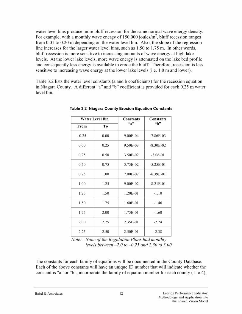
water level bins produce more bluff recession for the same normal wave energy density. For example, with a monthly wave energy of 150,000 joules/m2, bluff recession ranges from 0.01 to 0.20 m depending on the water level bin. Also, the slope of the regression line increases for the larger water level bins, such as 1.50 to 1.75 m. In other words, bluff recession is more sensitive to increasing amounts of wave energy at high lake levels. At the lower lake levels, more wave energy is attenuated on the lake bed profile and consequently less energy is available to erode the bluff. Therefore, recession is less sensitive to increasing wave energy at the lower lake levels (i.e. 1.0 m and lower). Table 3.2 lists the water level constants (a and b coefficients) for the recession equation in Niagara County. A different “a” and “b” coefficient is provided for each 0.25 m water level bin.

Table 3.2 Niagara County Erosion Equation Constants

Water Level Bin

From To

Constants “a”

Constants “b”

-0.25 0.00 9.00E-04 -7.86E-03

0.00 0.25 9.50E-03 -8.30E-02

0.25 0.50 3.50E-02 -3.06-01

0.50 0.75 5.75E-02 -5.25E-01

0.75 1.00 7.00E-02 -6.39E-01

1.00 1.25 9.00E-02 -8.21E-01

1.25 1.50 1.20E-01 -1.10

1.50 1.75 1.60E-01 -1.46

1.75 2.00 1.75E-01 -1.60

2.00 2.25 2.35E-01 -2.24

2.25 2.50 2.50E-01 -2.38

Note: None of the Regulation Plans had monthly levels between –2.0 to –0.25 and 2.50 to 3.00

The constants for each family of equations will be documented in the County Database. Each of the above constants will have an unique ID number that will indicate whether the constant is “a” or “b”, incorporate the family of equation number for each county (1 to 4),



Baird & Associates

12

and the water level bin (0.00 to 0.25 m). For example, the column heading for the water level bin –2.00 to –1.75 will be ‘a1n200n175’ and ‘b1n200n175’. The 1 indicates the family of equation number, the three digit numbers separated by n’s specify the water level bin in centimeters (cm) and the n points out that this is a negative water level bin. Therefore, water level bin 1.25 to 1.50 will have ID numbers a2p125p150 and b2p125p150. The p specifies that this is a positive water level bin and the 2 points out that this family of equation number 2.

The predictive equations have been applied to three reaches that correspond to locations with detailed COSMOS model simulations for 101 years. Table 3.3 shows the error at each reach between the modeled and predicted results for the four different hydrographs, 1958D with deviations, 1958D without deviations, Pre-Project and Plan 1998.

Table 3.3 Niagara County Prediction Equation Summary (note: Predicted=Equations, Modeled=COSMOS)

1958D with deviations 1958D without deviations

Reach

AARR (m/year

)


Predicted Recession

(m)

Modeled Recession

(m)

% Error

Predicted Recessio

n (m)

Modeled Recession

(m)

% Error

1181 0.86 Shallow 81.82 76.35 7.2% 94.20 85.64 10%

1152 0.30 Intermediate 29.71 28.38 4.7% 34.34 32.54 5.5%

1194 0.59 Deep 56.14 60.77 -7.6% 64.62 62.99 2.6%

Table 3.3 (con’t)

Pre-Project Plan 1998

Reach

AARR (m/year

)


Predicted Recession

(m)

Modeled Recession

(m)

% Error

Predicted Recessio

n (m)

Modeled Recession

(m)

% Error

1181 0.86 Shallow 100.54 105.95 -5.1% 80.26 73.10 9.8%

1152 0.30 Intermediate 37.10 35.23 5.3% 29.13 27.5 4.6%

1194 0.59 Deep 68.97 67.46 2.2% 55.06 59.57 -7.6%



Baird & Associates

13

The maximum error between the actual COSMOS results and the predictive equations is 10% and in several cases it is less than 5%. Although an additional level of detail (i.e. more equations) may improve the predictive capabilities of the equations, we believe that an error of ±10% is reasonable. The SVM will be able to screen plans, rank them, and quantify their economic impact. Further, the predictive equations will be verified against the COSMOS model and the FEPS in Year 4 of the study, which will provide some QA/QC. And, once the Climate Change and Stochastic Net Basin Supplies are included in the analysis, the predictive equations will be more robust below 0.0 and above 1.25 m.

3.4 Sandy Erosion

Prediction equations were not developed for erosion at sandy sites around Lake Ontario since sandy beach recession and/or accumulation rates cannot be easily determined. The historic annual average recession rates were used to predict the erosion at sandy sites around the lake. These AARR values capture the long-term behavior of the beach and do not account for the drastic changes a beach might experience after a storm.

3.5 SVM Application

3.5.1 Cohesive

The Shared Vision Model will evaluate monthly erosion. Each cohesive calculation requires a monthly water level, monthly normal wave energy, a historic AARR, and constants “a” and “b”. The relationships between each parcel and the relational databases are presented in a flow chart and as a graphic in Figure 3.7.

Prior to the actual calculations, the user must select the geographic extents for the analysis. For example: a reach, a single county, or the entire New York shoreline of Lake Ontario. In the FEPS, the user has the option to select counties, or a range of reaches.

The next step is to select only reaches that are classified as a cohesive shoreline, such as high glacial till bluffs, marine clay bluffs and low banks. The reaches classified in these three broad groups are given the 10x, 11x, 12x, and 16x numbers in the “ShoreType” field of the Reach Database. For example, a composite bluff with sand content of 0 to 20% is classified as 104. The sandy and wetland shorelines will not be modeled with this methodology.

Reach 1194, shoretype 104, in Niagara County will be used to illustrate this procedure for the first month of 1958D with deviations. The monthly water level for 1958D with deviations for January 1900, which can be found in the water level database, is 0.37m above chart datum. The database indicates that Reach 1194 is in Porter Township,



Baird & Associates

14

corresponds to WAVAD ID 1021, Family of Equations (FEQ) 1 and has an AARR of 0.59 m/year.

Select Regulation Plan and Spatial Extents for the

Analysis(i.e. reaches or

county)

ParcelDatabase

Assessed ValueDistance to BluffProtection Type

Reach

ReachDatabase

AARRFamily of Equations

WAVAD IDTownship

TownshipDatabase

'Distance to Existing Protection'

County

CountyDatabase

"a" and "b" coeff.Cost of Protection

Cost Trucked Sand

Wavad Point Database

Monthly Wave Energy for each WAVAD ID

Water Level Database

Weekly and Monthly Mean Water Levels for

all Regulation Plans

Figure 3.7a Flow Chart and Diagram of Relational Database for Erosion Equations

The Wavad Energy Database indicates that the normal wave energy for ID 1021 in January, 1900 is 75,736 Joules. The township database indicates that Porter Township is part of Niagara County. The water level elevation obtained from the database is in the 0.25 to 0.50m bin. Therefore, constants a and b have id numbers a1p025p050 and b1p025p050 respectively. These fields, which can be found in the County Database,



Baird & Associates

15

have values of 3.50E-02 and -3.06-01 respectively. The predicted recession for Plan 1958D with deviations at Reach 1194 for January 1900 is therefore:

(3.50E-02 x LN(75,736) + (-3.06E-01)) x 0.59 = 0.051m

This process will be carried out for each successive month at every cohesive reach around Lake Ontario. The cumulative recession for each reach should be determined by summing the predicted erosion for each month together. This cumulative recession will be used in the economic calculations. The total 101-year predicted recession for Plan 1958D with deviations at reach 1194 is 56.14m.

3.5.2 Sandy

Sandy erosion calculations will be carried out at reaches that are classified as sandy shoreline, such as Baymouth Barrier Complex, Sandy Beach / Dune Complex and Coarse Beaches. The reaches classified in these three broad groups are given the 13x, 14x and 15x, numbers in the “ShoreType” field of the Reach Database. For example, a gravel beach is classified as 151.

In Niagara County, Reach 1177 has shoretype classification 141 - Sandy Beach / Dune (relict deposits, areas with no new deposition). The AARR for this reach is 0.88m/year. Therefore, over a 101-year period the beach will erode 88.9m (0.88m/year x 101 years). This erosion rate will be the same for different water level plans since sufficient data is not available to relate water levels, waves and erosion. A relationship between water levels, waves and erosion/accumulation could be developed by taking very regular beach surveys and calculating the amount of sand lost or recovered for each period. This is out of the scope of this study and therefore, only the long-term observed recession and/or accumulation rates for Regulation Plan 1958D with Deviations can be used for this study.



Baird & Associates

16

4.0 ECONOMICS

Two economic methods are being used to quantify the sandy and cohesive erosion impacts around Lake Ontario: 1) Method I uses the Future Liability of Shore Protection for unprotected parcels with a house or other structures, and 2) Method II decreases the original assessed value of the undeveloped parcel based on the percentage of lost land due to erosion at the end of the simulation (i.e. 101 years). These economic methods are applied to each reach on a parcel by parcel basis. Parcels that already feature an existing shoreline protection structure will be treated under a different Performance Indicator. The different parcel classifications, the methods used at each parcel, and a description of the two methods are provided below.

4.1 Parcel Classes

There are four general combinations for the front row parcels based on shoreline protection and whether a house/building is present on the lot (developed vs. undeveloped):

• Unprotected shoreline without a house • Unprotected shoreline with a house • Protected shoreline without a house • Protected shoreline with a house

Parcel databases were initially obtained from the counties and often extended several kilometers inland, which is well beyond the zone of impact for the Erosion PI. Therefore, only the parcels within approximately a 100 m buffer of the shoreline were attributed in the GIS and included in the relational databases.

For residential areas, this generally includes the first two rows of parcel for the erosion impact assessment. For rural and agricultural areas, the parcels are larger and often only the first row of parcel is required to extend 100/200 m inland of the shoreline. Considering the four parcel conditions above and the potential occurrence of second row of parcels that may be impacted, there are 12 potential combinations that must be considered for the Erosion PI. These combinations are summarized in Table 4.1. The first four scenarios consider only front row parcels. Therefore, only the four cases listed above are considered. Conditions 5 to 8 focus on the second row of parcels with a house, while conditions 9 to 12 represent all potential combinations for second row parcels without a house or other building.

The economic method required at each combination is also listed in Table 4.1. Economic calculations are not required on first or second row parcels where shore protection is present, since it was assumed that the shore protection will be maintained for the duration



Baird & Associates

17

of the simulation (i.e. 101 years). Economic calculations are also not required for second row parcels that have a parcel in front of them with a house, since it has been assumed that the front row parcel will eventually build protection and therefore the second row parcel will never be exposed to erosion hazards.

Table 4.1 Erosion PI Methods for Different Parcel Combinations



Baird & Associates

18

4.2 Method I – Future Liability of Shore Protection

4.2.1 Conditions of Use – Developed Parcels

Method I will only be applied when there is a house present on an unprotected parcel. When a house is present on a parcel a number greater than zero will be present in the DistToBluff_M field in the Parcel Database and it is selected for the calculations. There are two conditions when the parcel is not selected: 1) if DistToBluff_M is equal to zero, the parcel has not been attributed for erosion because it is outside the zone of impacts for the erosion assessment, and 2) if there is no house, -9999 is used for the DistToBluff_M and the parcel is not selected (i.e. undeveloped parcels are not armored with shoreline protection).

Unprotected parcels are classified as 400 in the Protection Type field of the Parcel Database and these parcels are selected. Level 3 shore protection, which is poorly constructed or poorly maintained, does not provide long term protection. Therefore, these structures are ignored by the Erosion PI, the parcels are assumed to erode for the recession calculations, and the parcel are also selected. The shore protection classification uses a three digit numbering scheme. Level 3 is represented by a 3 in the final digit (XX3) in the Protection Type field of the Parcel Database.

Condition 1 and 6 from Table 4.1 will use Method I to quantify economic impacts of erosion. Method II is applied to condition 2 and 10. Condition 5 and 9 relate to second row parcels that featured an unprotected front row with a house. Since we assume that the front row parcel will eventually be protected, the second row parcel will never be exposed to erosion hazards and therefore, these parcels are not included in the calculations. Additional documentation for not selecting the remaining conditions are provided in Table 4.1.

4.2.2 Evaluation Methods

Method I will quantify the impacts of erosion using the Future Liability of Shore Protection. When evaluating different hydrographs or regulation plans, the method assumes that shoreline protection will eventually be constructed to mitigate the erosion hazard associated with bluff recession (i.e. the home owner incurs the liability of construction shoreline protection rather then letting their investment fall into the lake).

The cost of the shoreline protection structure will always be the same for different Regulation Plans. For cohesive erosion sites, the only difference between the plans will be “when” the liability is incurred in the future. For example, plans that accelerate erosion may force the riparian land owner to build protection in 10 years, versus 50 years for a plan that reduces erosion. The further the liability or cost of constructing the protection into the future, the greater the benefits for the riparian land owner considering



Baird & Associates

19

the compounding effects of interest. For example, if we assume that a $60,000 shoreline protection structure will eventually be required and a long term interest rate of 3.1% is applied, an initial investment of $32,582 is required if the protection is required in 20 years versus only $17,693 if the liability of constructing the shoreline protection is delayed until 40 years in the future.

Shore protection will be built at the same time for sandy erosion sites since a relationship between water level and erosion rate have not been determined. Sandy erosion sites will therefore not influence the selection of plans.

The steps required to complete the above calculations for different Regulation Plans are outlined below:

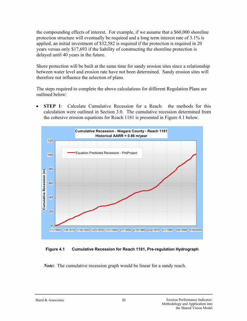
• STEP 1: Calculate Cumulative Recession for a Reach: the methods for this calculation were outlined in Section 3.0. The cumulative recession determined from the cohesive erosion equations for Reach 1181 is presented in Figure 4.1 below.

Cumulative Recession - Niagara County - Reach 1181Historical AARR = 0.86 m/year

0

20

40

60

80

100

120

1/1/1900 1/8/1910 1/16/1920 1/23/1930 1/31/1940 2/7/1950 2/15/1960 2/22/1970 3/1/1980 3/9/1990 3/16/2000

Cum

ulat

ive

Rec

essi

on (m

)

Equation Predicted Recession - PreProject

Figure 4.1 Cumulative Recession for Reach 1181, Pre-regulation Hydrograph

Note: The cumulative recession graph would be linear for a sandy reach.



Baird & Associates

20

• STEP 2: Calculate Distance to Required Protection for each individual Parcel: the distance that the shoreline erodes until it is necessary to build shore protection. Parcel 22.33-2-84 will be used as an example

DistanceRequiredProtection =DistToBluff_M – DistanceToProtection =40.66 m – 30.0 m =10.66 m

Distance to Bluff and Distance to Protection are both measured from the building’s lakeward edge. Distance to Bluff is a variable in the Parcel Database and Distance to Protection is a variable in the Township Database and based on the average distance of all buildings in a Township that already feature protection. In other words, it represents local preferences, physical conditions (high bluff vs. low bank), and social-economic considerations. Note: If the Distance to Protection is greater than the Distance to Bluff, then shore protection is required immediately. The economic impact is equal to the Absolute Cost of Protection.

• STEP 3: Calculate Geotime: time (years) in the future when shoreline recession is

equal to or greater than Distance to Required Protection, rounded to a whole year.

Geotime =This is a look-up function for cohesive reaches based on the string created in Step 1 (time,cumulative recession). When cumulative recession is equal to or greater than Distance to Required Protection, read and save date (month/year)

Cumulative recession in 6/1/1912 is 10.64 m, which is less than DistanceRequiredProtection (10.66 m). However, in 7/1/1912, cumulative recession is 10.66 m, which is equal to DistanceRequiredProtection.

Since the simulation started in 1/1/1900, the time in years, rounded to a whole number is 13 (Jan. to June, round down, July to Dec., round up).

For sandy reaches, Geotime = DistanceRequiredProtection/Historic AARR

Note: If cumulative recession is never greater than Distance to Required Protection during simulation time or if the geotime for sandy reaches is greater than 101-years, then no shore protection will be required. There would be no economic impact for that parcel.



Baird & Associates

21

• STEP 4: Calculate Absolute Cost of Protection:

AbsoluteCostProtection =Frontage_M * CostProtection =52.59 m * $2,000/m =$105,180

Frontage is defined as the width of the parcel at top of bank or shoreline and can be found as a variable in the parcel database. Cost of Protection is a variable in the County Database and assumes a typical Level 2 structure is built (i.e. seawall).

• STEP 5: Calculate Investment by Riparian for Future Shore Protection:

Initial Investment = Absolute Cost of Protection (1 + Interest Rate)Geotime =$105,180/(1+2%)13 =$81,307.56

4.2.3 Comparison of Plans

Figure 4.2 Required Investment for Future

Liability of Shore Protection

Steps 1 through 5 provide an overview of the methods used to calculate the economic impacts of erosion on parcels with a house that have not been protected for the Pre-Project hydrograph. The results for the other plans and using an interest rate of 3.1% are presented graphically in Figure 4.2.

The economic standards for the study stipulate that the benefits and costs of alternative Regulation Plans should be normalized to the results for 1958D with deviations. Figure 4.3 presents the normalized initial investment requirements for shore protection at Parcel 22.33-2-84. Plan 1998 represents a benefit of approximately $5,000, while the Pre-Project outflows would result in an additional cost of $19,000.



Baird & Associates

22

Figure 4.2 Required Investment for Future Liability of Shore Protection

4.3 Method II

4.3.1 Conditions of Use – Undeveloped Parcels

Method II will only be applied when the parcel is unprotected and there is no house present. When there is no house present on a parcel either -9999, -9987 or –9994 will appear in the DistToBluff_M field in the Parcel Database. If these parcels are unprotected (Protection = 400) or feature Level 3 protection, they represent Condition 2 in Table 4.1 and are selected for Method II.

Second row parcels that are undeveloped must also be considered. Second row parcels feature a “0” in the ProtectionType field of the Parcel database, since it is impossible to protect a second row parcel. There are four scenarios for the front row parcel, as outlined in Table 4.1 (Conditions 9 to 12), when the second row parcel is undeveloped. Only Condition 10 meets the criteria for Method II, which occurs when the front row parcel is undeveloped and unprotected. The economic assessments assumes this parcel will not be protected and erode during simulation time. If the entire first row parcel is eroded, the undeveloped second row parcel would also be impacted during the simulation.

4.3.2 Evaluation Methods

The steps required to complete the above calculations for different Regulation Plans are outlined below. Parcel 32.18-1-2 is used as an example for Pre-Project water levels:



Baird & Associates

23

• STEP 1: Calculate Cumulative Recession for Reach 1194: the methods for this calculation were outlined in Section 3.0. The cumulative recession for Reach 1194 is 69.53 m for 101 years of simulation time. The results are presented in Figure 4.1.

• STEP 2: Check how much of the parcel depth is eroded during simulation time. In

some cases, the parcel may be completely eroded, which would result in a 100% loss of assessed value.

% Parcel eroded? If CumRec > or = LandDepth_M, parcel eroded 100%

Then, economic loss = CumulativeLand (assessed value of undeveloped parcel)

If LandDepth_M > CumRec, go to step 3

Example for Parcel 32.18-1-2:

102.54 > 69.53, therefore go to step 3

Figure 4.1 Cumulative Recession for Reach 1181, Pre-regulation Hydrograph

Note: The cumulative recession graph would be linear for a sandy reach.

• STEP 3: Calculate remaining parcel depth and percentage after simulation time. Note, we assume each parcel is rectangular, so it is not necessary to complete an area calculation to determine the change parcel size)



Baird & Associates

24

RemainingDepth =LandDepth_M – CumRec


=102.54 – 69.53 =33.01 m

% RemainingDepth =RemainingDepth / LandDepth_M * 100


=33.01 / 102.54 * 100

=32.19%

• STEP 4: Modify assessed value for undeveloped parcel (land only)

modCumulativeLand =CumulativeLand * %RemainingDepth


=$12,000 * 32.19%

=$3,863.08



Baird & Associates

25

5.0 SUMMARY

The variables required for erosion and economic calculations are summarized below.

5.1 Required Data

In order to evaluate erosion impacts with the SVM, certain data will be required from all of the databases. Table 5.1 lists all of the required variables necessary for erosion impact analysis and the databases they are found in.

Table 5.1 Required Data for the Evaluation of Cohesive Erosion Impacts

Database Variable Unit

Water Level Monthly Water Level Elevation (corresponding to each plan)

Meters with respect to chart datum

County/Regional Municipalityp

Constant, a Constant

Constant, b Constant

Cost of Protection (Cost Protection)

US Dollars

Township Distance to Protection Meters

Normal Wave Energy Monthly Normal Wave Energy (corresponding to WavadID)

Joules

Reach AARR Meters/Year

Shoretype (Sandy or Cohesive) N/A

Parcel Distance to Bluff Meters

Frontage Meters

****Red indicates variables required for erosion prediction, Blue indicates variables required for economic calculations.



Baird & Associates

26

5.2 Fields and flags for Parcel Database

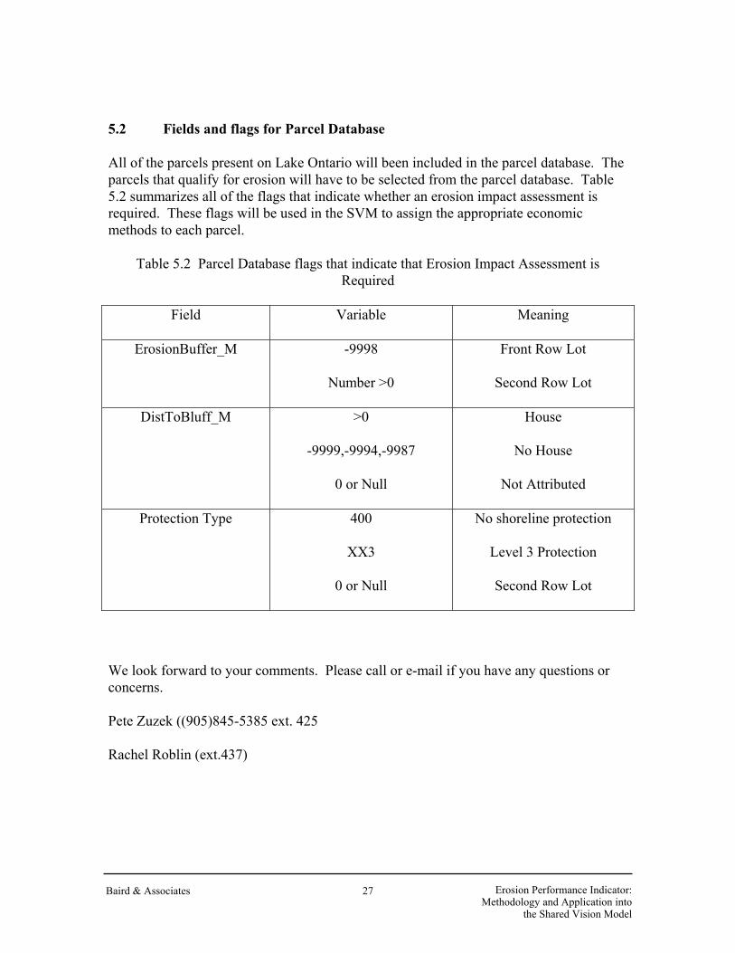
All of the parcels present on Lake Ontario will been included in the parcel database. The parcels that qualify for erosion will have to be selected from the parcel database. Table 5.2 summarizes all of the flags that indicate whether an erosion impact assessment is required. These flags will be used in the SVM to assign the appropriate economic methods to each parcel.

Table 5.2 Parcel Database flags that indicate that Erosion Impact Assessment is Required

Field Variable Meaning

ErosionBuffer_M -9998

Number >0

Front Row Lot

Second Row Lot

DistToBluff_M >0

-9999,-9994,-9987

0 or Null

House

No House

Not Attributed

Protection Type 400

XX3

0 or Null

No shoreline protection

Level 3 Protection

Second Row Lot

We look forward to your comments. Please call or e-mail if you have any questions or concerns.

Pete Zuzek ((905)845-5385 ext. 425

Rachel Roblin (ext.437)



Baird & Associates

27

erosion performance indicator: methodology … methods... · describes the svm goals and the...

Documents