1

Error Bands for Impulse ResponsesChristopher A. Sims

and

Tao Zha

July 1995

Revised, July 1998

We show how correctly to extend known methods forgenerating error bands in reduced form VAR’s tooveridentified models. We argue that the conventionalpointwise bands common in the literature should besupplemented with measures of shape uncertainty, and weshow how to generate such measures. We focus on bandsthat characterize the shape of the likelihood. Such bandsare not classical confidence regions. We explain thatclassical confidence regions mix information aboutparameter location with information about model fit, andhence can be misleading as summaries of the implicationsof the data for the location of parameters. Becauseclassical confidence regions also present conceptual andcomputational problems in multivariate time seriesmodels, we suggest that likelihood-based bands, ratherthan approximate confidence bands based on asymptotictheory, be standard in reporting results for this type ofmodel.

2

I. Introduction

In interpreting dynamic multivariate linear models, impulse response functions are of centralinterest. Presenting measures of the statistical reliability of estimated impulse responses is there-fore important. We will discuss extensions of existing methods for constructing error bands thataddress some important practical issues.

• It has been conventional in the applied literature to construct a 1− α probability intervalseparately at each point of a response horizon, then to plot the response itself with theupper and lower limits of the probability intervals as three lines. The resulting band isnot generally a region that contains the true impulse response with probability 1− α anddoes not directly give much information about the forms of deviation from the pointestimate of the response function that are most likely. In Section VI we suggest a way toprovide such information.

• While there is a widely used, correct algorithm1 for generating error bands for impulseresponses in reduced form VAR models, it is not easy to see how to extend it tooveridentified structural VAR’s, and some mistaken attempts at extension have appearedin the literature. In Section VIII we show how correctly to make this extension and howto use numerical methods to implement it.

But before we present the details of our proposed methods for dealing with these issues, weneed to take up some conceptual issues. The error bands we discuss are meant to characterize theshape of the likelihood function, or of the likelihood function multiplied by the type of referenceprior widely used in reporting results to a scientific audience. The importance of characterizingthe shape of the likelihood, because of the likelihood’s central role in any decision-making use ofa statistical model, should not be controversial. The main critiques of likelihood-based inference(e.g. Loève (1988)) argue against the likelihood principle, the claim that only the likelihood needbe reported, not against the importance of reporting the shape of the likelihood. Computing andreporting these likelihood-characterizing intervals is a substantial challenge in itself, anddeserves more attention in applied work.

There are valid arguments for reporting more than the likelihood, and classical confidenceintervals can be thought of as constructed from the likelihood plus additional information aboutoverall model fit that is needed for model criticism. However, confidence intervals mixlikelihood information and information about model fit in a confusing way: narrow classicalconfidence bands can be indicators either of precise sample information about the location ofparameters or of strong sample information that the model is invalid. It would be better to keepthe two types of information separate.

Section II lays out in more detail the general argument for reporting separately likelihoodshape and fit measures, rather than reporting confidence intervals.

Section III defines “impulse responses” and the class of models we are considering.

1 Distributed in the RATS manual since the earliest versions of that program.

3

Section IV discusses the problems raised by the fact that we are forming measures ofprecision of our inference about vector-valued functions of a vector of parameters, with thedimensionality of both vectors high. For likelihood-describing error bands, these problems arejust the need to make some choices about practical details of implementation. Attempts toinstead form confidence regions run into serious conceptual problems in this situation.

It is not possible, even in principle, for the time series models we are interested in, toconstruct classical confidence intervals for impulse responses with exact small-samplejustification. There are a variety of approaches to obtaining approximate confidence intervalsthat grow more accurate in some sense as sample size increases. Many of these approaches thathave been used in practice have the same degree of justification in first-order classical asymptotictheory as the practice of using Bayesian posterior probability intervals as if they were confidenceintervals. There are particular bootstrap methods (little-used in applied time series research) thathave improved second-order asymptotic properties in theory, though not in practice according toMonte Carlo studies. Section V discusses these methods and the problems in implementingthem.

Examples in Sections VII and VIII.B illustrate the performance of our suggested methods andprovide some comparisons with other approaches.

II. Likelihood Shape vs. Coverage Probability

Formal decision theory leads, under some regularity conditions, to the conclusion thatrational decision rules have the form of Bayesian rules.2 Following Hildreth (1963), we mightthink of scientific reporting as the problem of conveying results of analysis to an audience thatmay have diverse prior beliefs about parameters and diverse loss functions, but accept a commonstatistical model. Reporting is not decision-making, and therefore makes no use of subjectiveprior beliefs. Instead it relies on the likelihood principle3: all evidence in a sample about theparameters of the model is contained in the likelihood, the normalized p.d.f. for the sample withthe data held fixed and the parameters allowed to vary. Scientific reporting is then just theproblem of conveying the shape of the likelihood to potential users of the analysis.

It does not seem reasonable, though, to suppose that very often a wide audience accepts astatistical model as certainly true, rather than as an interesting hypothesis or plausibleapproximation. Readers who are interested in the model and its parameters, but might want alsoto consider other models, will need more than the likelihood function. To compare the fit of oneparametric model to another for the same data, one needs to construct the likelihood function forthe grand model made up of the two, with a discrete parameter that chooses between the twomodels. To construct this overall likelihood, we need to use both the separate model likelihoodsand their relative levels. If a proper4 Bayesian reference prior is being used, this can be done bypresenting the posterior p.d.f.’s for the two separate models, which will usually be close to theirlikelihoods in shape, and the posterior probabilities of the two models. Geweke (1995), for

2 Such a result is called a Complete Class Theorem. See Ferguson (1967).3 See Berger and Wolpert (1988)4 I.e. a probability distribution, rather than a “density function” that does not integrate to one.

4

example, suggests reporting such information. But no use of a prior is necessary to report thisinformation. The same information is contained in the two separate likelihoods themselves,together with any statistic that determines their relative heights – e.g. the ratio of p.d.f. values atsome particular point in the sample space. Of course if the set of models to be considered is notknown in advance, then the levels of the p.d.f. values are needed for all the models reported.

The likelihood function contains the sample information about parameters of the model,while the additional information about level of the p.d.f. contains information about fit of thismodel relative to possible competitor models. A classical confidence interval, together with itscoverage probability, does not depend only on the likelihood. Therefore, in decision-makingwith a trusted model, use of a classical confidence interval and coverage probability must ingeneral lead to suboptimal decisions. However, in scientific reporting, as we have just argued, itmay be important to convey information beyond that in the likelihood. Therefore it cannot beargued that with the likelihood available, confidence intervals are redundant. It can be argued,though, that with the likelihood and a measure of overall fit both available, confidence intervalsare redundant.

A. Simple Examples

Consider a simple situation where a single random variable X is observed that takes on onlyinteger values 1, 2, or 3. It is distributed either according to model A or model B in Table 1.Only X = 2 is compatible with both models, though it is a rare observation for either model.The implications of the model for inference are intuitively clear: If X = 1 is observed, model Ais true, with certainty; if X = 3 is observed, model B is true, with certainty, and if X = 2 isobserved, observing X has not told us anything about whether the true distribution is A or B. Theodds ratios in the last column of the table capture these implications of the data precisely. Theimplications of observing X are well expressed by a 100% confidence interval, based onlikelihood ratios, which contains A alone if X = 1, B alone if X = 3, and both A and B if X = 2 .These are also 100% Bayesian posterior probability intervals under any prior distribution thatputs non-zero weight on both models. Because the likelihood ratio (the ratio of the likelihood ata particular parameter value to the likelihood at its maximum) is always either 1 or 0 in thisexample, this 100% interval is the only likelihood-ratio based confidence interval available forthis example.

Table 1: Empty or Trivial Confidence SetsA B

X P(X|A) LR P(X|B) LR LR 100% conf. set Simple 99% conf. set Flat prior odds ratio1 0.99 1.00 0 0.00 (A) (A) ∞2 0.01 1.00 0.01 1.00 (A,B) () 13 0 0.00 0.99 1.00 (B) (B) 0

Confidence intervals based on likelihood ratios have the advantage that they tend to havenearly the same shape as a minimum-length (or minimum-volume, in multi-parameter contexts)posterior probability interval under a flat prior. They also can be shown to have some classicaloptimality properties. But any collection of tests at a given exact significance level 1− α ,indexed by all the points in the parameter space, implies an exact confidence region. In thisexample it might be appealing to test model A and model B, rejecting A if X = 3 and B if X = 1.This leads to the exact 99% confidence region listed in the 7th column of Table 1. This interval

5

agrees with the 100% interval except when X = 2 , in which case the 99% interval is empty,instead of containing the whole parameter space.

How can we interpret a statement, having seen X = 2, that “with 99% confidence” the modelis neither A nor B? If we seriously believe that possibly neither model is correct, this kind ofstatement might make sense. The confidence interval has been constructed from likelihood ratiosbetween each model A and B and an implicit third model – that which puts equal probability onall three values of X. This is just a way of describing what has been done here – for eachparameter value (A or B) collecting the points in the sample space with lowest probabilitydensity (relative to an equal-weight probability measure over the three possible observations) toform the rejection region. The empty confidence interval when X = 2 is observed does suggest,if we take this implicit third model as a serious possibility, that abandoning both models A and Bmight be justified.

If one wants information about the possibility that no parameter value in the model or modelsbeing considered performs well, the fact that a confidence interval can provide this, and nolikelihood-based interval (such as a Bayesian posterior probability interval) can do so, may be anadvantage of a confidence interval. However, it is nearly universal in applied work thatconfidence intervals are interpreted mainly as informing us about the location of the parametervalues, not about the validity of the model. An empty confidence interval is only an extreme caseof a narrow confidence interval. Confidence intervals can turn out to be misleading as indicatorsof the precision of our knowledge about parameter location because they confound suchinformation with information about overall model fit.

Consider the example of Table 2, in which there is again a single, integer-valued observedrandom variable X for which there are two candidate probability models, A and B. This time, thetwo models are very similar, with the probabilities of each of the 3 possible values of X differingby no more than .001. A likelihood-ratio based confidence set, displayed in column 6 of thetable, produces a hard-to-interpret amalgam of information about fit and information aboutparameter location. It is never empty, but it contains only model B when X is 2 and only modelA when X is 3. A statement, on observing X = 3, that “with 99% confidence the model is A”makes no sense as a claim about the precision of our ability to distinguish between models A andB based on the observation. The interval is “short” because of poor overall fit of the model, notbecause of precision of the data’s implications about choosing between A and B.

Table 2: Spuriously “Informative” Confidence Sets

X P(X|A) LR P(X|B) LR LR 99% conf. set Flat prior odds ratio1 0.979 1.00 0.979 1.00 (A,B) 1.002 0.01 0.91 0.011 1.00 (B) 0.913 0.011 1.00 0.01 0.91 (A) 1.10

The likelihood in these simple two-model cases is information equivalent to the flat-priorodds ratio in the last column of the tables. Reporting it would correctly show for the Table 2case, no matter what X were observed, that seeing X had provided little information about whichmodel, A or B, is the truth. But if we see X = 3 and simply cite the odds ratio of 1.1 in favor ofA, we fail to convey the fact that X = 3 was unlikely under either model A or B. It would bebetter to report the two separate p.d.f. values .011 and .01, or the odds ratio 1.1 and themarginalized likelihood ( the sum of the p.d.f. over the two models, .021).

6

The confidence intervals in these examples give misleading information about shape of thelikelihood only in low-probability samples. This reflects a general proposition, that an exact1− αb g% confidence interval must have Bayesian posterior probability greater than 1− nα on a

set of sample values with probability, under the marginal distribution over observations impliedby the prior distribution and the model jointly, of at least n n−1b g , for any n >1. In other

words, a stochastic interval with high confidence level must in most samples also have highposterior probability. The proposition is symmetric: a stochastic interval that has posteriorprobability 1− α in every sample must have a coverage probability greater than or equal to1− nα for a set of parameter values that has prior probability of at least n n−1b g .5

Thus if confidence intervals or regions with confidence levels near 1 are easy to compute,they can be justified as likely to be good approximations, with high probability, to directcharacterizations of likelihood shape. But where, as in the models we consider, directcharacterizations of likelihood shape are easier to compute, there seems to be little reason toundertake special effort to compute confidence regions rather than direct measures of likelihoodshape. Also, for characterizing likelihood shape, bands that correspond to 50% or 68% posteriorprobability are often more useful than 95% or 99% bands, and confidence intervals with suchlow coverage probabilities do not generally have posterior probabilities close to their coverageprobabilities.

B. A Time Series Example

To show how these points apply in a time series model we consider the simple model

y t y t t t Tb g b g b g= − + =ρ ε1 1, ,..., . (1)

We assume ε is i.i.d. N(0,1), independent of y’s dated earlier. Suppose a sample produces $ .ρ = 95

and $ .σ ρ = 046 , both likely values when ρ =.95 . An exact6 finite-sample 68% confidence interval

5 The proof of these propositions follows from the observation that the following two things arethe same: i) the expectation over the prior distribution of the (classical) conditional coverageprobabilities given parameter values, and ii) the expectation over the marginal distribution of thedata (with parameters integrated out using the prior) of the posterior probability that theparameter is in the set given the data. These are two ways to calculate the probability, under thejoint probability measure on parameters and data, of the event that the parameter lies in therandom set.6 Since the classical small sample distribution was calculated by Monte Carlo methods on a gridwith spacing .01 on the ρ-axis and with 2000 replications, "exact" should be in quotes here, butthe accuracy is good enough for these examples. The method was to construct, for each ρ, 2000artificial samples for y generated by (1) with T=60, variance of ε equal to 1, and y(0)=0. (Thesame sequence of ε's was used for all ρ's on each draw of an ε sequence.) For each ρ, an

empirical distribution of the log likelihood ratio (LR) $ ( )ρ ρ− ⋅ −∑b g2 21y t was constructed and

the 16% and 84% quantiles of the empirical distribution calculated. Then a classical 68%confidence interval can be constructed in a particular sample as the set of all ρ’s for which the

7

for ρ, based on the distribution of ( $ )ρ ρ σ ρ− 2 2 (the log likelihood ratio), is (0.907, 0.998). A

Bayesian flat-prior posterior 68% probability region is (.904, .996). Here the confidence regionis not very misleading. It has flat-prior posterior probability .67 instead of .68, which is not a bigerror, and is shifted upward by .003 at the lower end and .002 at the upper end, which is a shift ofonly about 5% of its length. The likelihood levels at the upper and lower bounds of the intervaldiffer by only about 6%.

The difference between confidence intervals and integrated-likelihood intervals becomessomewhat larger if we consider 95% intervals. For this probability level, the Bayesian interval is(0.860, 1.040), while the LR-based exact confidence interval is (0.865, 1.052). This intervalshows noticeable distortion at the upper end. The likelihood is twice as high at the lower end ofthe interval as at the upper. The interval therefore is representative of the shape of posteriorbeliefs only for a prior with p.d.f. increasing over the interval so that ρ = 1.052 is twice as likelyas ρ =.865 . The interval does have posterior probability under a flat prior of .95 (to two-figureaccuracy), however.

The LR-based exact confidence interval we consider here is intuitively attractive and hassome justification in classical theory, but as usual there is no unique classical confidence interval.It is commonly proposed, (see Rothenberg and Stock (1998), e.g.), that intervals be based insteadon the signed likelihood ratio (the signed difference in log likelihoods). Such intervals tend forthis model to be more sharply asymmetric than ordinary LR intervals. In this simple case theconfidence intervals based on signed LR are (0.917, 1.013) for 68% confidence and (0.869,1.064) for 95% confidence. Though these intervals are further biased upward as likelihooddescriptions than the LR-based intervals, they have flat-prior posterior probabilities of .68 and.95.

Cases of empty confidence intervals or misleadingly short confidence intervals are likely toarise when the parameter space is restricted to ρ ∈[ , ]01 . If the confidence interval is based on

the distribution of the signed difference between the log likelihood at ρ and the log likelihood atthe unrestricted MLE $ρ (which can exceed 1, of course), and is built up from equal-tailed tests,empty 68% confidence intervals have a probability of 16% and empty 95% confidence intervalshave a probability of 2.5% when ρ = 1.7 If instead the distribution of the ratio of the likelihood

at ρ to the likelihood at its maximum on [0,1] is used to generate the interval, the interval willnever be empty, but it will be shorter than can be justified by the likelihood shape in thesesamples where the unrestricted MLE lies above 1, because of the same kind of phenomenondisplayed in Table 2 above. When the true ρ is 1 for example, an observation as high as

log LR statistic lies between the 16% and 84% quantiles appropriate for that ρ. The samemethod was applied in the other example calculations in this section.7 This is an exact result, by construction. The confidence interval lies entirely above ρ = 1 in

samples for which $ρ ρ− ⋅ −∑b g yt 12 is negative and below the lower α 2b g% tail of its

distribution conditional on ρ = 1. But by construction this occurs in just α 2b g% of samples

when in fact ρ = 1.

8

$ .ρ = 10387 has about a 1% chance of occurring, and a typical associated σ ρ is .0394. With such

a sample, the exact classical 68% confidence interval based on the signed LR, calculatednumerically on a grid with ρ’s spaced at .001, includes only three points, defining the interval(.998,1), and the 95% interval expands only to (.966,1). But the likelihood has the formdisplayed in Figure 1, which clearly does not concentrate as sharply near 1 as these confidenceintervals would suggest. Such a high $ρ is unlikely for any ρ in [0,1], but not as much more

likely for ρ’s of .97 compared to ρ’s of 1 as the confidence interval would suggest. A flat-priorposterior 68% interval for ρ is (.975,1) and the 95% probability interval is (.944,1).

Figure 1: Likelihood over (0,1) with $ .ρ = 10387, σ ρ =.0394

0.86 0.88 0.9 0.92 0.94 0.96 0.98 10

0.1

0.2

0.3

0.4

0.5

0.6

0.7

0.8

0.9

1

The conclusion these examples are meant to illustrate is that flat-prior Bayesian 1− αprobability intervals, based purely on the likelihood, are often very close to exact ( )1− α %confidence intervals, and that in those samples where they differ, confidence intervals can bequite misleading as characterizations of information in the sample about parameter location.

III. Multivariate Dynamic Models

Consider a model of the form

g y t y t y t k t( ), ( ),..., ( )− − =1 β εc h b g (2)

where

∂ − −∂

≠g y t y t y t k

y t

( ), ( ),...,

( )

10

b gc hβ, (3)

so that the equation defines y t( ) as a function of ε βt y t y t kb g b g b g, ,..., ,− −1 . We assume that

ε( )t is independent of y t s( )− , all s>0, and has p.d.f. h ⋅ Ωc h . Under these conditions (3) allows

us to write a p.d.f. for y y T( ),..., ( )1 conditional on y y k( ),..., ( ), ,0 1− + β Ω , which we will label

9

p y y T y y k( ),..., ( ) ( ),..., ( ), ,1 0 1− + β Ωc h . (4)

It is common but not universal practice to treat (4) as the likelihood function. It is actuallythe likelihood function only if the distribution of y y k( ),..., ( )0 1− + does not depend on unknown

parameters, or depends only on unknown parameters unrelated to β and Ω. If (2) is consistentwith y being ergodic, then it is natural to take the ergodic marginal distribution ofy t y t k( ),..., ( )− , which of course in general depends on β and Ω, as the distribution fory y k( ),..., ( )0 1− + . This is then combined with (4) to produce a p.d.f. for the full vector ofobservations y k y k y T( ), ( ),..., ( )− + − +1 2 . There are three reasons this is not often done: itoften makes computations much more difficult; it requires that we rule out, or treat as a separatespecial case, non-stationary (and thus non-ergodic) versions of the model; and it may not beplausible that the dynamic mechanism described in (2) has been in operation long enough, inunchanged form, to give y y k( ),..., ( )0 1− + the ergodic distribution. The last two points arerelated. A non-stationary model has no ergodic distribution. A near-non-stationary model mayhave an ergodic distribution, yet it may imply that the time required to arrive at the ergodicdistribution from arbitrary initial conditions is so long that imposing the ergodic distribution ony y k( ),..., ( )0 1− + may be unreasonable.

Bayesian inference would ideally use the ergodic distribution for the initial conditions at pa-rameter values well within the stationary region of the parameter space, then shift smoothly overto a distribution less connected to β and Ω as the non-stationary region is approached. Such amodel is likely to be application-dependent, however, and in the remainder of this paper we treat(4) as the likelihood. We also hold initial conditions fixed in generating Monte Carlo samples ofy y T( ),..., ( )1 when we evaluate classical coverage probabilities.8

Much of our analysis will focus on the case where g is linear in its first y argument with anidentity coefficient matrix and also linear in β, and h is Gaussian. Under these conditions the loglikelihood is quadratic in β, so the likelihood itself is Gaussian in shape, in small and largesamples, for stationary and non-stationary models.

For a general model of the form (2), there is ambiguity about how “impulse responses” oughtto be defined. Here, though, we consider only models such that g is linear in its y arguments, sothat the response c sij ( ) of y t si ( )+ to ε j t( ) is easily and unambiguously defined. By solving (2)

8 On this latter point we differ from Kilian (1998a). Conditioning on initial data values informing the likelihood or in constructing estimators (on which point Kilian’s practice matchesours) amounts to ignoring potential information in the initial observations. Conditioning on themin doing Monte Carlo simulations of the data-generation process amounts to recognizing thedistinction between initial conditions that generate more and less informative samples. If theinitial y’s show unusually large deviations from their steady-state values, the sample is likely togenerate unusually sharp information about the parameters. It does not make sense to calculatecoverage probabilities that average across informative and uninformative samples when it is easyto take account of the fact that we have been lucky (or unlucky) in the initial conditions of theparticular sample at hand.

10

recursively, we can solve for y t s( )+ as a function of ε ε ε( ), ( ),..., ( )t s t s t+ + −1 andy t y t k( ),..., ( )− −1 . Then

c sy t s

tiji

j

( )( )

( )= +∂

∂ε(5)

depends only on β, not y or ε, and can be calculated by elementary matrix operations. Note that,though the impulse responses as defined here coincide with the coefficients of the movingaverage representation (MAR) for stationary, linearly regular models, they are also defined fornonstationary models where no MAR exists.

If we write the linear model in terms of the lag operator, as

A L y t tb g b g( ) = ε , (6)

then the impulse responses are the coefficients in the infinite-order polynomial in the lag operator

C L A Lb g b g= −1 , where the inverse is restricted to involve only positive powers of L and is

interpreted as an operator on the field of finite-order polynomials in the lag operator. Such aninverse exists for any finite-order A with A0 full rank, regardless of the characteristic roots of A,though of course it may imply coefficient matrices Cs that fail to converge to zero as s→ ∞ .The mapping from the coefficients in A, the autoregressive form of the model, to those in C, isone-one. Because A is finite-order (in the models we consider) and C is not, there is a sense inwhich A is a more economical characterization of the model than is C. On the other hand,because the elements c tij b g of the Ct matrices tend to behave, as function of t, like the data that

is being modeled, the properties of the model are often more easily grasped intuitively byviewing plots of c tij b g ’s than by viewing tables of a tij b g ’s.

Though the mapping from the full A operator to the full C operator is one-one, the mappingfrom the aij ’s to a particular c tij b g is complicated. Generally the mapping is not one-one, even if

we consider a collection c t t Hij ( ), ,...,= 1 in which H is the same as the dimension of the vector

of all the free parameters in A.9 This engenders some complications in defining error bands, and(especially) in defining confidence intervals, for c tij b g .

IV. Dimensionality

Because impulse responses are high dimensional objects, describing error bands for them ischallenging. The best approaches to describing them will differ to some extent acrossapplications, but we describe some widely applicable approaches in Section VI below. In this

9 To see this point, consider a first-order model with A I A L= − 1 and A1 m m× . If A1 has

Jordan decomposition A P P11= −Λ , with Λ diagonal, then cij ⋅b g depends on the i’th row of P, the

j’th column of P−1, and all the elements of the diagonal of Λ, but on no other aspects of A1.

Clearly this leaves room for many A1 ’s to deliver exactly the same cij ⋅b g .

11

section we discuss the difficulties created by the fact that multivariate time series models havehigh-dimensional parameter spaces.

A complete characterization of a subset of a parameter space in a 150-dimensional parameterspace (which would not be unusually large for a multivariate time series model) would be toocomplicated to be useful. Instead we try to capture substantively important characteristics oferror band sets with a few lower-dimensional statistics and plots. For example, we may focusattention on a few impulse responses that are important for characterizing the effects of a policyaction on the economy. With a given Bayesian prior distribution, characterizing the probability,given the data, of a set of possible values for a given impulse response – e.g. the probability thatc t a b tij ( ) [ , ], ,...,∈ = 1 4 – is a straightforward exercise: One integrates the posterior p.d.f. with

respect to all the parameters of the model over the set of parameter values that deliver cij ’s

satisfying the restrictions.

For confidence intervals, the high dimensional parameter space raises a different kind ofproblem. The same impulse response function cij can arise from two different A L( ) operators.

The coverage probability of any stochastic set in the space of cij ’s, now matter how generated,

will depend not just on cij itself, and will therefore be different for different A Lb g ’scorresponding to the same cij . Therefore no exact confidence set for cij is possible.

This point, that coverage probabilities often depend on nuisance parameters and that thiscauses problems, is an old one. Some writers define the confidence level of a random interval asthe minimum over the parameter space of the coverage probability.10 This corresponds (becauseof the duality between confidence regions and hypothesis tests) to the standard definition of thesize of a statistical test as the maximum over the parameter space of the probability of rejectionunder the null. However, as has recently been emphasized in work by Dufour (1997), Faust(1996), and Horowitz and Savin (1998), this approach is unsatisfactory, as it leads often to asituation where there are no non-trivial confidence intervals, even asymptotically. In practice,researchers use confidence intervals or regions justified by asymptotic theory, in the sense thatthe coverage probability converges to its nominal level as sample size increases, pointwise ateach point in the sample space. Often this can be accomplished by simply computing coverageprobabilities at estimated values of nuisance parameters.

In small samples, though, this approach can lead to serious distortion of the shape of thelikelihood. For example, there can be a wide range of values of a nuisance parameter ν, all withhigh likelihood, with widely different implications for the coverage probability of a confidenceset. If we replace ν by a single estimated value, we may obtain an unrepresentative value for thecoverage probability. In this same situation, Bayesian posterior probability intervals wouldinvolve integration over ν, rather than choice of a single ν, which better represents the actualimplications of the data. With the likelihood spread evenly over ν’s with different implications,Bayesian results could be sensitive to the prior. But a thorough description of the likelihood,including if necessary consideration of more than one reference prior, can make this situation

10 Zacks (1971), e.g. defines confidence level this way, while Wilks (1962) seems to consider insmall samples only cases of coverage probabilities uniform over the whole parameter space.

12

clear. Furthermore, often the likelihood dominates the prior, so that over the range of ν’s ofinterest most readers would agree that the prior is nearly flat.

V. Asymptotics, Approximation, the Bootstrap

We have already cited the fact that Bayesian posterior probability intervals have asymptoticjustification as confidence intervals in time series models of the type we consider. This result,like many on which confidence intervals for these models have been based, actually applies onlyto situations where the model is known to be stationary. The result is easiest to see in the specialcase of an unrestricted reduced form VAR, i.e. a model with A I0 = . In that case the likelihoodconditioned on initial observations is Normal-Inverse-Gamma in shape, centered at the OLSestimate, with a covariance matrix that even in finite samples is exactly the covariance matrix ofthe asymptotic distribution of the estimates. The marginal distribution for the Aj ’s is then easily

seen to converge to the shape of the same limiting normal distribution to which the samplingdistribution of the OLS estimates converges. Of course this then implies that all differentiablefunctions of the coefficients of A, including the Cj ’s, have posterior distributions that are

asymptotically normal, and match the sampling distributions of the same functions of the OLSestimate of A.

For more general stationary linear models a maximum likelihood estimator of the coefficientsin A, or a pseudo-maximum likelihood estimator based on a Gaussian likelihood when thedisturbances are not Gaussian, or another GMM estimator, will each converge, under mildregularity conditions, to a joint normal distribution. The posterior distribution of the parameters,conditional on the estimators themselves and their estimated asymptotic covariance matrix (notconditional on the full sample, outside the Gaussian case), should in large samples be wellapproximated by taking the product of the prior p.d.f. with the asymptotic normal p.d.f. as anapproximate joint p.d.f. from which to construct the posterior. But since in large samples thelikelihood dominates the prior, we can treat the prior as constant in this approximation. Thecomputation of the posterior amounts to fixing the estimator and its estimated covariance matrix,then treating the asymptotic p.d.f. of the sample as a function of the coefficients in A inconstructing the posterior p.d.f. for A. This will make the posterior distribution have the sameshape as the asymptotic sampling distribution of the estimator. Because the asymptoticdistribution is symmetric and affected by the parameters only via a pure location shift, confidenceregions then coincide with posterior probability intervals. Proofs of these results, with carefulspecification of regularity conditions, are in Kwan (1998).

The mappings from Aj coefficients to Cj coefficients can be analytically differentiated, so

that normal asymptotic distributions for the A coefficients can be translated into normalasymptotic distributions for the C coefficients. Details have been provided, e.g., in Lutkepohl.(1990) and Mittnik and Zadrozny (1993)11. However the mapping from A to Cj is increasingly

nonlinear as j increases, so that the quality of the approximation provided by this type ofasymptotic theory deteriorates steadily with increasing j in any given sample. Eventually as jincreases (and this occurs for fairly low j in practice) the norm of the variance of Cj begins to

11 This approach has been used by, e.g. Poterba, Rotemberg and Summers (1986).

13

behave as λ− j , where λ is the root of A L( ) = 0 that is smallest in absolute value. This means

that when the point estimate of λ exceeds one, error bands shrink at the rate λ− j for large j, evenwhen there is in fact substantial uncertainty about the magnitude of λ. This is an importantsource of inaccuracy, and results in poor behavior in Monte Carlo studies of error bandsgenerated this way. (See Kilian (1998b)).

Another way to generate confidence intervals with the same first-order asymptoticjustification as use of Bayesian intervals as confidence intervals is to use simple bootstrapprocedures. Perhaps because Bose (1988) has shown that bootstrap calculations provide a higherorder of asymptotic approximation in the distribution of the estimator in a stationary finite-orderautoregressive model, some researchers have the impression that simple methods for translatingan estimate of the distribution of the estimator at the true parameter value into a confidenceinterval must improve the accuracy of confidence intervals, but this is not the case. Someapplied studies12 have used what might be called the “naive bootstrap”, but which Hall (1992)and we in the rest of this paper will call the “other-percentile” bootstrap interval. An initial

consistent estimate $A is generated, and Monte Carlo draws are made from the model with

A A= $ , to generate a distribution of estimates $$A about $A . To generate a confidence band for

c tij ( ) , the $$A ’s are mapped into a distribution of corresponding $ ( )c tij ’s, and the 1− αb g%

“confidence interval” is formed by finding the upper and lower α 2b g% tails of the distribution

of the $ ( )c tij ’s. This procedure clearly amplifies any bias present in the estimation procedure. In

our simple time series example of section II.B, the procedure would produce intervals shifteddownward relative to the Bayesian intervals, instead of the slight upward shift produced by exactclassical intervals.

In a pure location problem, where we observe X f X~ − µb g and the p.d.f. f is asymmetric,

the standard method of generating a confidence interval is to find the upper and lower α 2b g%

tails of the p.d.f. f, say a and b, and then use the fact that, with µ fixed and X varying randomly,

P a X b P X b X a< − < = − < < − = −µ µ α1 . (7)

If we used the other-percentile bootstrap and made enough Monte Carlo draws to determine theshape of f exactly, we would use not the X b X a− −,b g interval implied by (7), but instead

X a X b+ +,b g– that is, the interval in (7) “flipped” around the observed point X. It may seem

obvious that, having made our bootstrap Monte Carlo draws, we should use the interval in (7),not the other-percentile bootstrap interval. Indeed, the interval X b X a− −,b g implied by (7) is

called the “percentile interval” by Hall (1992) and treated by him as the most natural bootstrapinterval. In the pure location-shift context, it produces an interval with flat-prior Bayesian

12 This approach has been used by Runkle (1987). Blanchard and Quah (1989) and Lastrapes andSelgin (1994) use a modification of it that makes ad hoc adjustments to prevent the computedbands from failing to include the point estimates.

14

posterior probability equal to its nominal coverage probability, and is therefore a usefuldescriptor of the likelihood function.

But we can also imagine a setting in which we do not have a location shift problem with non-Gaussian distribution, in which instead there is an underlying Gaussian (or otherwisesymmetrically distributed) location-shift problem, that has become non-Gaussian through anunknown nonlinear transformation. That is, we observe X and wish to form a confidence interval

for µ, as before, but now X g Z= b g and µ θ= gb g , where Z N~ ,θ σ 2d i , g is monotone, and we

do not know necessarily know g. It can be shown that in this situation the other-percentilebootstrap interval would give exactly the right answer, in the sense that it would produce aninterval with flat-prior Bayesian posterior probability matching its nominal coverage probability.

In time series problems, for parameters that imply stationary data, estimates of thecoefficients in A Lb g are asymptotically normal, but biased in small samples. The coefficients in

Cj are functions of the coefficients in A Lb g , with the degree of nonlinearity in the mapping

increasing with j. One might expect then that bias considerations could dominate for j near zero,making Hall’s percentile intervals work best, while the effects of nonlinear transformation woulddominate for large j, making “other-percentile” intervals work best. But there is no obvious,general method of using bootstrap simulations to produce confidence intervals whose length andskewness accurately reflect asymmetry in sample information about the Cj ’s.

Kilian in several papers (Kilian (1998a), Kilian (1998b), e.g.) has argued for use of other-percentile bootstrap intervals with bias correction.13 While there is no argument available thatsuch intervals are more accurate in coverage probability asymptotically than other bootstrapapproaches or than Bayesian probability intervals, the bias-correction does tend to remove themost important source of bad behavior of other-percentile intervals in time series models.

There are ways to construct bootstrap confidence intervals that make them asymptoticallyaccurate to second order, instead of only to first order. One such method is that presented in Hall(1992) as “symmetric percentile-t”. Another is that presented in Efron and Tibshirani (1993) as“ BCα ” 14. The Hall intervals are symmetric about point estimates, so they cannot provide

information about asymmetry in the likelihood. The Efron and Tsibshirani estimates areburdensome to compute. Both have behaved badly in Monte Carlo studies of multivariate timeseries models (Kilian (1998b)).

As should already be clear, we believe error bands that are descriptive of the likelihood are tobe preferred, in scientific reporting, to classical confidence regions with known coverageprobabilities, even when the latter can be constructed. Nonetheless we report in our examplesbelow some measures of the behavior of bootstrap-based approximate confidence intervals. Weuse Kilian’s bias-adjusted bootstrap method (Kilian (1998a)) and the commonly applied other-

13 But note that Kilian is primarily just correcting the initial estimator for bias. See Hall (1992),p.129 for some elaboration of the point that what is called “bias correction” in the literature ofbootstrapped confidence intervals is not correction of the bootstrapped estimator for bias.14 This interval is an other-percentile interval adjusted for “bias” and “acceleration”.

15

percentile method. As we have noted, both can be justified as good approximations to Bayesianintervals under particular assumptions on the way the distribution of the observed statisticsdepends on the parameter. Both are relatively straightforward to compute.

VI. Better Measures of Uncertainty about Shape of Responses

Common practice is to compute a one-dimensional error band $ ( )c t tij ijb g ± δ for each

t H= 0,..., , then plot on a single set of axes the three functions of time $c t tij ijb g b g− δ , $c tij b g , and

$c t tij ijb g b g+ δ , attempting to show the reader both the point estimate of the response and an

indication of the range of uncertainty about the form of the response. It is extremely unlikely ineconomic applications that the uncertainty about c tij b g is independent across t, and indeed this is

probably a good thing. Readers probably tend to think of the plotted upper and lower confidenceband points as representing cij ⋅b g functions at the boundaries of likely variation in cij . If the

uncertainty about c were in fact serially independent across t, the smoothly connected upper andlower confidence bands would represent extremely unlikely patterns of deviation of cij from $cij .

But in models fit to levels of typically serially correlated economic time series, uncertainty aboutc is usually itself positively serially correlated, so thinking of the $ ( )c t tij ijb g ± δ plots as possible

draws from the distribution of c is not as unreasonable as it might seem.

Nonetheless, models are sometimes fit to data that is not very smooth, or to differenced data,and even for data in levels the “connect the dots” bands can turn out to be misleading. To bettercharacterize the uncertainty, one can turn to representing the cij ⋅b g functions in a better co-

ordinate system than the vector of their values at t H= 0,..., . If the c tij t

Hb gn s =0 vector were

jointly normal with covariance matrix Ω, the obvious coordinate system would be formed byprojections on the principal components of Ω, and one can use this coordinate system even if thec’s are not jointly normal.

To implement this idea, one computes a pseudo-random sample from the distribution of cij ,

using it to accumulate a first and second moment matrix. From these, one computes theestimated covariance matrix Ω of the H-dimensional cij matrix and calculates its eigenvector

decomposition

W WΛ Ω′ = , (8)

where Λ is diagonal and ′ =W W I. Any cij can now be represented as

c c Wij ij k kk

H

= + •=

∑$ γ1

, (9)

where we are treating cij as an H-dimensional column vector, $cij is the estimated mean of cij ,

and W k• is the k’th column (i.e. k’th eigenvector) of W. Random variation in cij , which

represents our uncertainty about cij given observation of the data, is generated by randomness in

16

the coefficients γ kl q . By construction, the variance of γ k is the k’th diagonal element of the

matrix Λ in (8), i.e. the k’th eigenvalue of Ω.

In models of economic data, it is likely that the largest few eigenvalues of Ω account for mostof the uncertainty in cij . We can, in such a case, give a much more complete description of

uncertainty about cij than is available in a “connect-the-dots” error band by presenting just a few

plots, displaying, say, $c t W tij k kb g b g± ⋅• λ to represent an approximate 68% probability band for

the k’th variance component, or $ .c t W tij k kb g b g± ⋅• 196 λ for approximate 95% intervals. Unlike

the functions of t plotted in connect-the-dots error bands, these plots show cij functions that lie

in the boundary of the Gaussian confidence ellipsoid, when the distribution of cij is Gaussian.

This method, though possibly useful in practice as a time-saver, is still unsatisfactory, as weknow that the cij ’s are often not well approximated as jointly normal, particularly for their values

at large t. The linear eigenvector bands we have described will always be symmetric about $cij ,

for example, while the posterior distribution usually is not. It is often important to know whenthe posterior is strongly asymmetric.

So we can improve on the above method by conducting another round of Monte Carlosimulation, or, if the first round, used to form Ω, has been saved, by making another pass throughthe saved draws. This time, we tabulate the 16%, 84%, 2.5% and 97.5% (say) quantiles of theγ k corresponding to the largest eigenvalues of Ω. The γ k for a particular draw of cij is easily

computed as W ck ij• , where Wk• is the k’th row of W. The two functions of t, $ ,.cij k+ γ 16 and

$ ,.cij k+ γ 84 , if λ k is one of the largest eigenvalues, will each show a likely direction of variation

in cij , and their different magnitudes of deviation from $cij will give an indication of asymmetry

in the likelihood or posterior p.d.f.

One further step up in sophistication for these measures is possible. Often it is important tothe use or the interpretation of a result how several cij ’s, for different i and j, are related to each

other. For example, it is often thought that plausible patterns of response of the economy to adisturbance in monetary policy should have interest rates rising, money stock falling, outputfalling, and prices falling. When we look at the error band for the response of output to amonetary shock and see that, say, it looks plausible that the output decline could be much greaterthan the point estimate, we really need to know whether the stronger output decline implies anyviolation of the sign pattern that implies the shock is plausibly treated as a policy shock.

This kind of question can be answered by stacking up several cij ’s into a single vector, then

applying eigenvalue decomposition methods suggested above. It may not be as widely useful toapply these methods to cij ’s jointly as it is to apply them to single cij ’s, because there is not as

strong a presumption of high correlations of c tij b g values across i and j as there is across t.

However, where it turns out that a few eigenvalues do dominate the covariance matrix of asubstantively interrelated set of cij ’s, this sort of exercise can be very helpful.

17

Before proceeding to examples, we should note that the ideas in this section are not limited inapplication to impulse responses. They apply wherever there is a need to characterize uncertaintyabout estimated functions of an index t and there is strong dependence across t in the uncertaintyabout the function values. This certainly is the case when we need to characterize uncertaintyabout the future time path of an economic variable in a forecasting application, for example. Italso will apply to some cases in which non-parametric kernel estimates of regression functions,p.d.f.’s, or the like are being presented.

VII. Application to Some Bivariate Models

We consider two examples of bivariate models based on economic time series. Though theyare unrealistically simple, they make it feasible to do a wide range of checks on the methods, inorder to give a clearer impression of the feasibility of the methods we suggest, their value intransmitting information, and the degree to which they give results resembling or differing fromother possible methods for generating error bands.

First we consider a triangularly orthogonalized reduced-form VAR with four lags fitted toquarterly data on real GNP and M1 over 1948:1-1989:3. Figure 2 shows pointwise flat-priorposterior probability intervals for this mode’s impulse responses.15 For both the response of Y toits own shocks, in the upper left, and the response of M1 to its own shocks, in the lower right,there is notable skewness in the bands, with the 95% bands especially extending farther up thandown. Figure 3 shows 68% other-percentile intervals, without bias-correction. Note that for theresponses of GNP and M1 to their own innovations, these other-percentile bands are quiteasymmetric, shifted down toward 0. This reflects bias in the estimator, and it does not makesense to treat these intervals, which accurately reflect the shape of the distribution of theestimates about the truth, as characterizing reasonable beliefs about parameter location. Withbias-adjustment, as displayed in Figure 4, other-percentile bootstrap intervals show the samequalitative pattern as the Bayesian intervals, but are more skewed, somewhat wider, and with atendency to splay out at the longer time horizons.16

15 For both these models we use 1000 Monte Carlo draws in generating Bayesian or bootstrapintervals for a given data set, and 600 draws of data sets in constructing coverage probabilities.16 Note that our implementation of bias-adjusted other-percentile intervals does not follow Kilianin his ad hoc adjustments of sample draws to eliminate non-stationary roots. Our view is thatmildly non-stationary estimates may be realistic, so that it is usually inappropriate to truncate theparameter space at or just inside the boundary of the stationary region. We also condition oninitial observations in generating bootstrap draws, which Kilian does not.

18

Figure 2: Pointwise .68 and .95 Posterior Probability Bands,Y-M Model

Responses to

0

2.06y

M1

4 8 16 32-.55

0

3.01

4 8 16 32

19

Figure 3: 68% and 98% Other-Percentile BootstrapBands, Y-M Model

Responses to

0

1.77y

M1

4 8 16 32-.42

0

2.26

4 8 16 32

Figure 4: 68% and 95% Bias-Corrected Bootstrap Bands, Y-M Model

Responses to

20

-.57

0

2.82y

M1

4 8 16 32-1.31

0

3.61

4 8 16 32

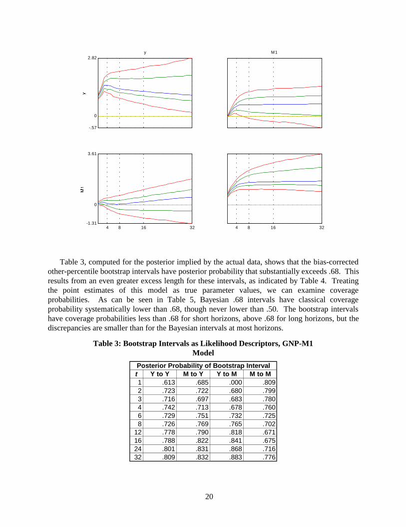
Table 3, computed for the posterior implied by the actual data, shows that the bias-correctedother-percentile bootstrap intervals have posterior probability that substantially exceeds .68. Thisresults from an even greater excess length for these intervals, as indicated by Table 4. Treatingthe point estimates of this model as true parameter values, we can examine coverageprobabilities. As can be seen in Table 5, Bayesian .68 intervals have classical coverageprobability systematically lower than .68, though never lower than .50. The bootstrap intervalshave coverage probabilities less than .68 for short horizons, above .68 for long horizons, but thediscrepancies are smaller than for the Bayesian intervals at most horizons.

Table 3: Bootstrap Intervals as Likelihood Descriptors, GNP-M1Model

Posterior Probability of Bootstrap Int ervalt Y to Y M to Y Y to M M to M1 .613 .685 .000 .8092 .723 .722 .680 .7993 .716 .697 .683 .7804 .742 .713 .678 .7606 .729 .751 .732 .7258 .726 .769 .765 .702

12 .778 .790 .818 .67116 .788 .822 .841 .67524 .801 .831 .868 .71632 .809 .832 .883 .776

21

Note: Monte Carlo standard error of a .68 frequency with 1000 draws is .015. Bootstrapintervals have nominal coverage probability of .68. The samples are random draws withinitial y’s both 1.

Table 4: Comparison of Interval Lengths, GNP-M1 Model

Ratios of Mean Lengths: Bayesian/Bootstrapt Y to Y M to Y Y to M M to M1 1.022 1.016 1.000 1.0202 .995 .988 1.015 .9833 .967 .961 .982 .9494 .938 .929 .945 .9186 .895 .880 .892 .8728 .841 .829 .836 .828

12 .759 .762 .750 .75616 .716 .730 .708 .72124 .652 .691 .644 .67732 .603 .661 .599 .647

Table 5: Bayesian and Bootstrap Intervals as Confidence Regions,GNP-M1 Model

Bootstrap Interval Coverage Proba bilities Bayesian Interval Coverage Proba bilitiesY to Y M to Y Y to M M to M t Y to Y M to Y Y to M M to M

.432 .687 .000 .360 1 .595 .668 .000 .595

.540 .678 .717 .502 2 .618 .672 .685 .543

.603 .692 .685 .592 3 .577 .687 .643 .557

.625 .670 .688 .622 4 .593 .690 .613 .518

.657 .702 .687 .653 6 .585 .677 .618 .523

.650 .713 .685 .655 8 .560 .670 .610 .510

.682 .717 .697 .675 12 .555 .642 .627 .518

.703 .732 .707 .687 16 .557 .623 .608 .513

.712 .730 .742 .712 24 .570 .642 .617 .517

.725 .742 .748 .750 32 .602 .632 .610 .520

Note: Monte Carlo standard error of a .68 frequency with 600 draws is .019. Bootstrap intervals havenominal coverage probability of .68. Bayesian intervals are flat-prior, equal-tail, .68 posteriorprobability intervals.

For this model, the pointwise bands carry nearly all shape information, because the firstcomponent of the covariance matrix of each impulse response is strongly dominant. We can seethis in Figure 5, which displays error bands for the first component of variation in each impulseresponse. The bands in this figure are very similar to the pointwise bands shown in Figure 2.The main difference is a tendency for the component bands to be tighter for t close to 0. For eachof the four response functions in these graphs, the largest eigenvalue accounts for over 90% ofthe sum of the eigenvalues. The second eigenvalue accounts for between 2.3% and 32%, and thethird for no more than 1.1%. Figure 6 shows the second component, which in this case seems tocorrespond to uncertainty about the degree to which the response is “hump-shaped”. We do notdisplay the third component because it is quite small. In this model, use of pointwise bands,together with what we guess is the usual intuition that uncertainty about the level, not the shape,of the response dominates, would lead to correct conclusions.

22

Figure 5: 1st Component: .68 and .95 Probability Bands, Y-M Model

0

2.00y

M1

4 8 16 32-.50

0

2.99

4 8 16 32

23

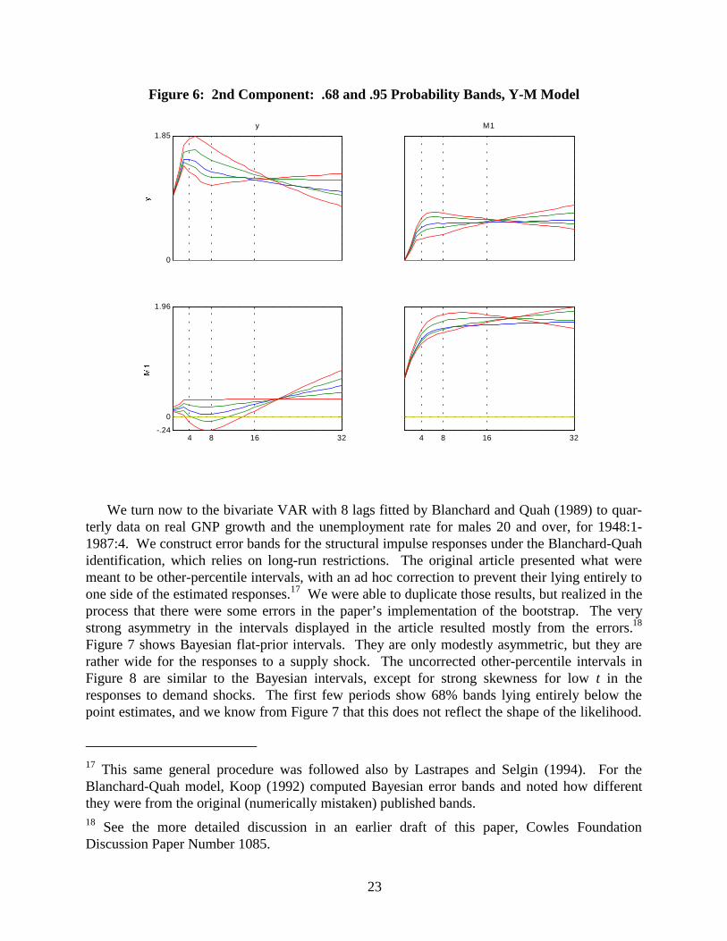
Figure 6: 2nd Component: .68 and .95 Probability Bands, Y-M Model

0

1.85y

M1

4 8 16 32-.24

0

1.96

4 8 16 32

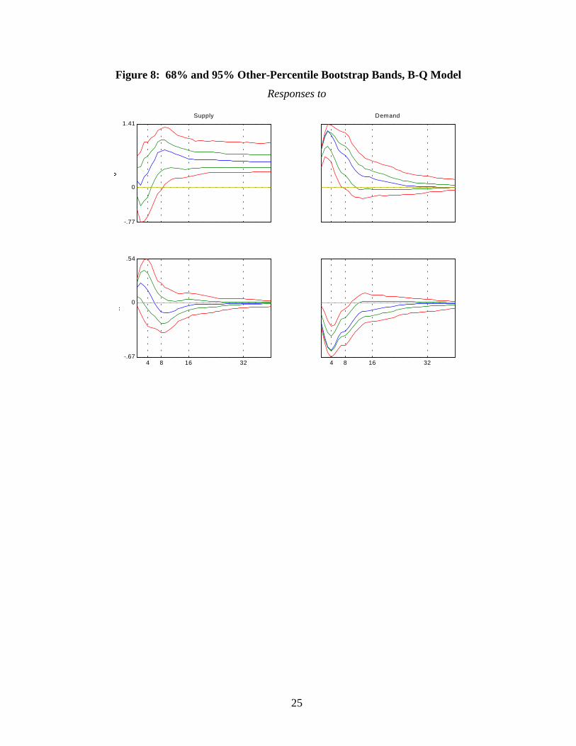
We turn now to the bivariate VAR with 8 lags fitted by Blanchard and Quah (1989) to quar-terly data on real GNP growth and the unemployment rate for males 20 and over, for 1948:1-1987:4. We construct error bands for the structural impulse responses under the Blanchard-Quahidentification, which relies on long-run restrictions. The original article presented what weremeant to be other-percentile intervals, with an ad hoc correction to prevent their lying entirely toone side of the estimated responses.17 We were able to duplicate those results, but realized in theprocess that there were some errors in the paper’s implementation of the bootstrap. The verystrong asymmetry in the intervals displayed in the article resulted mostly from the errors.18

Figure 7 shows Bayesian flat-prior intervals. They are only modestly asymmetric, but they arerather wide for the responses to a supply shock. The uncorrected other-percentile intervals inFigure 8 are similar to the Bayesian intervals, except for strong skewness for low t in theresponses to demand shocks. The first few periods show 68% bands lying entirely below thepoint estimates, and we know from Figure 7 that this does not reflect the shape of the likelihood.

17 This same general procedure was followed also by Lastrapes and Selgin (1994). For theBlanchard-Quah model, Koop (1992) computed Bayesian error bands and noted how differentthey were from the original (numerically mistaken) published bands.18 See the more detailed discussion in an earlier draft of this paper, Cowles FoundationDiscussion Paper Number 1085.

24

Bias correction has slight effects on these bands, as can be seen from Figure 9; in particular thestrong bias toward zero in the bands for responses to demand at low t is still present after bias-correction.

Figure 7: Pointwise: .68 and .95 Posterior Probability Bands, B-Q Model

Responses to

-.89

0

1.62Supply

Demand

4 8 16 32-.73

0

.62

4 8 16 32

25

Figure 8: 68% and 95% Other-Percentile Bootstrap Bands, B-Q Model

Responses to

-.77

0

1.41Supply

Demand

4 8 16 32-.67

0

.54

4 8 16 32

26

Figure 9: 68% and 95% Bias-Corrected Bootstrap Bands, B-Q Model

Responses to

-.79

0

1.46Supply

Demand

4 8 16 32-.70

0

.56

4 8 16 32

In contrast to the implications of Table 3 for the Y-M model, Table 6 shows that the bias-corrected bootstrap intervals are for the B-Q model not bad as indicators of posterior probability,except for a tendency to hold too little probability at low t in the responses to demand shocks.This reflects the spurious skewness already noted for those responses and t values. In this model,in contrast to the Y-M1 model, the Bayesian intervals and bias-corrected bootstrap intervals havealmost the same average lengths, as can be seen from Table 7. The lower posterior probabilityfor the bootstrap intervals at low t for responses to demand comes from the intervals beingmislocated, not from their being too short.

27

Table 6: Bootstrap Intervals as Likelihood Descriptors,Blanchard-Quah Model

Posterior Probabilities of Bootstrap Int ervalst Y to S U to S Y to D U to D

1 .710 .696 .452 .6442 .706 .715 .583 .6163 .701 .717 .655 .6114 .688 .712 .700 .6616 .693 .696 .712 .6738 .703 .698 .705 .731

12 .687 .718 .700 .69216 .693 .713 .689 .68424 .668 .714 .670 .67632 .655 .721 .707 .718

Note: Monte Carlo standard error of a .68 frequency with 1000 draws is.015. Bootstrap intervals have nominal coverage probability of .68.The samples are random draws with initial y’s both 1.

Table 7: Comparison of Interval Lengths, Blanchard-Quah Model

Ratios of Mean Lengths: Bayesian/Bootstrapt Y to S U to S Y to D U to D

1 1.009 1.004 .996 1.0082 1.005 1.001 .985 1.0063 .997 .999 .979 .9934 .990 .992 .979 .9846 .972 .981 .997 .9848 .962 .975 .991 .994

12 .972 .985 .995 .99916 .979 .983 1.005 1.01624 .976 .942 .984 1.00132 .963 .886 .958 .969

Note: Monte Carlo standard errors of these figures vary, but none are over .06.

If we take the estimated coefficients of the Blanchard-Quah model as the truth, we can checkcoverage probabilities for bootstrap and Bayesian intervals. Table 8 shows similar behavior forBayesian and bootstrap intervals by classical criteria. Both intervals tend to undercover for theGNP-to-demand response at short horizons, though the undercoverage is considerably worse forthe bootstrap interval. Both tend to overcover at long time horizons, with the tendency slightlyworse for the Bayesian intervals.

28

Table 8: Bayesian and Bootstrap Intervals as Confidence Regions,Blanchard-Quah Model

Bootstrap Interval Coverage Proba bilities Bayesian Interval Coverage Proba bilitiest Y to S U to S Y to D U to D t Y to S U to S Y to D U to D1 .657 .650 .050 .632 1 .653 .662 .273 .6722 .648 .653 .108 .425 2 .658 .655 .270 .6183 .647 .642 .225 .295 3 .650 .668 .372 .4624 .657 .642 .337 .297 4 .658 .660 .445 .4486 .678 .647 .550 .452 6 .642 .637 .615 .5058 .670 .672 .593 .525 8 .647 .623 .652 .600

12 .687 .705 .630 .635 12 .690 .705 .658 .63216 .728 .775 .645 .707 16 .752 .792 .693 .72524 .747 .845 .783 .780 24 .768 .860 .845 .85332 .737 .910 .928 .865 32 .760 .923 .952 .920

Note: Monte Carlo standard error of a .68 frequency with 600 draws is .019.Bootstrap intervals have nominal coverage probability of .68. Bayesian intervals areflat-prior, equal-tail, .68 posterior probability intervals.

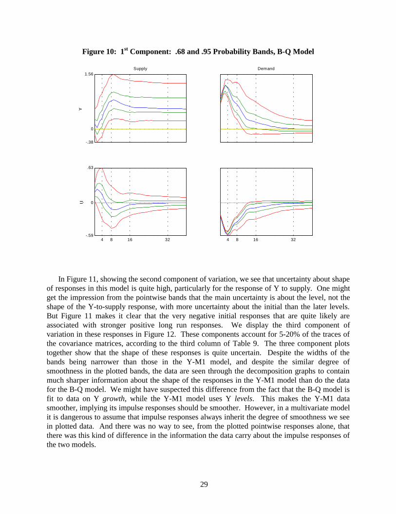
For this model, the first component of the covariance matrix accounts for much less of theoverall variation, especially for the responses to demand, as is shown in Table 9. Bands on thefirst component are shown in Figure 10. These bands have the same general shape as those inFigure 7, but are for the most part narrower, reflecting the fact that they describe only one, notcompletely dominant, component of variation. It is interesting that the Y-to-supply response hasa wider band on this first component for large t than one sees in the pointwise bands of Figure 7.This can only occur because of non-Gaussianity in the posterior distribution.

Table 9: Variance Decompositions for BQ Model Responses

0.7147 0.2029 0.0492 Y to supply

0.7487 0.1319 0.0654 U to Supply

0.6165 0.2002 0.0984 Y to demand

0.4555 0.2117 0.1835 U to demand

29

Figure 10: 1st Component: .68 and .95 Probability Bands, B-Q Model

-.38

0

1.56Supply

Demand

4 8 16 32-.59

0

.63

4 8 16 32

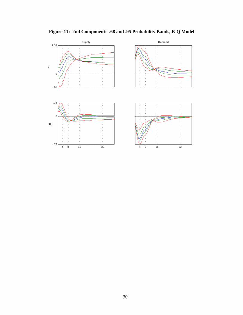
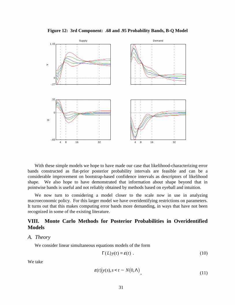
In Figure 11, showing the second component of variation, we see that uncertainty about shapeof responses in this model is quite high, particularly for the response of Y to supply. One mightget the impression from the pointwise bands that the main uncertainty is about the level, not theshape of the Y-to-supply response, with more uncertainty about the initial than the later levels.But Figure 11 makes it clear that the very negative initial responses that are quite likely areassociated with stronger positive long run responses. We display the third component ofvariation in these responses in Figure 12. These components account for 5-20% of the traces ofthe covariance matrices, according to the third column of Table 9. The three component plotstogether show that the shape of these responses is quite uncertain. Despite the widths of thebands being narrower than those in the Y-M1 model, and despite the similar degree ofsmoothness in the plotted bands, the data are seen through the decomposition graphs to containmuch sharper information about the shape of the responses in the Y-M1 model than do the datafor the B-Q model. We might have suspected this difference from the fact that the B-Q model isfit to data on Y growth, while the Y-M1 model uses Y levels. This makes the Y-M1 datasmoother, implying its impulse responses should be smoother. However, in a multivariate modelit is dangerous to assume that impulse responses always inherit the degree of smoothness we seein plotted data. And there was no way to see, from the plotted pointwise responses alone, thatthere was this kind of difference in the information the data carry about the impulse responses ofthe two models.

30

Figure 11: 2nd Component: .68 and .95 Probability Bands, B-Q Model

-.65

0

1.39Supply

Demand

4 8 16 32-.73

0

.35

4 8 16 32

31

Figure 12: 3rd Component: .68 and .95 Probability Bands, B-Q Model

-.27

0

1.43Supply

Demand

4 8 16 32-.65

0

.32

4 8 16 32

With these simple models we hope to have made our case that likelihood-characterizing errorbands constructed as flat-prior posterior probability intervals are feasible and can be aconsiderable improvement on bootstrap-based confidence intervals as descriptors of likelihoodshape. We also hope to have demonstrated that information about shape beyond that inpointwise bands is useful and not reliably obtained by methods based on eyeball and intuition.

We now turn to considering a model closer to the scale now in use in analyzingmacroeconomic policy. For this larger model we have overidentifying restrictions on parameters.It turns out that this makes computing error bands more demanding, in ways that have not beenrecognized in some of the existing literature.

VIII. Monte Carlo Methods for Posterior Probabilities in OveridentifiedModels

A. Theory

We consider linear simultaneous equations models of the form

Γ( ) ( ) ( )L y t t= ε . (10)

We take

ε( ) ( ), ~ ,t y s s t N< 0 Λb g , (11)

32

with Λ diagonal. We assume Γ0 to be non-singular, so that (10) provides a complete descriptionof the conditional distribution of y t( ) given y s s t( ), < and can be solved by multiplying through

on the left by Γ01− to produce the reduced form

B L y t u t( ) ( ) ( )= , (12)

in which B I0 = and u t( ) , while still uncorrelated with past y’s, has a covariance matrix whichis not in general diagonal, being given by

Σ Γ ΛΓ= ′− −0

10

1 . (13)

We assume the system is a finite-order autoregression, meaning that there is a k < ∞ such thatΓ j jB= = 0 for all j k> .

The p.d.f. for the data y y T( ),..., ( )1 , conditional on the initial observationsy k y( ),..., ( )− +1 0 , is proportional to q as defined by

q B S BT

, expΣ Σ Σb g b gd i= − 2 - trace12

-1 (14)

$ ; ( ) ( )u t B B L y tb g = (15)

S B u t B u t Bt

T

( ) $( , ) $( , )= ′=∑

1

. (16)

For a given sample, (14) treated as a function of the parameters B and Σ is the likelihoodfunction. Its form is exactly that of the likelihood for a regression with Gaussian disturbancesand strictly exogenous regressors, a classic model for which Bayesian calculations are well-discussed in the literature.19 The RATS program includes routines to implement Monte Carlodrawing from the joint distribution of B and Σ and use of those draws to generate a Monte Carlosample from the posterior distribution of impulse responses.20

19 See, e.g., Box and Tiao (1973), Chapter 8 for the theory.20 Box and Tiao (1973) recommend using a Jeffreys prior on Σ, which turns out to be

proportional to Σ − +m 12 . The packaged RATS procedure uses instead Σ − + +m ν 1

2 , where ν is the

number of estimated coefficients per equation. Phillips (1992) suggests using the joint Jeffreysprior on B and Σ, which in time series models (unlike models with exogenous regressors) is notflat in B. The Phillips suggestion has the drawback that the joint Jeffreys prior iscomputationally inconvenient and changes drastically with sample size, making it difficult forreaders to compare results across data sets. We therefore prefer the Box and Tiao suggestion inprinciple, though they point out (p. 44) that even in models with exogenous regressorsmechanical use of Jeffreys priors can lead to anomalies. In this paper, to keep our results ascomparable as possible to the existing applied literature, we have followed the RATSprocedure’s choice of prior.

33

The impulse responses for the model , defined by (5) above, are in this case the coefficientsof

B L− −10

1 12b gΓ Λ , (17)

where the Λ12 factor scales the structural disturbances to have unit variance, or equivalently

converts the responses so they have the scale of a response to a disturbance of “typical” (one-standard-deviation) size. Equation (13) gives us a relation among Σ, Γ, and Λ. Because Σ issymmetric, Γ0 and Λ have more unrestricted coefficients than Σ. An exactly identified VARmodel is one in which we have just enough restrictions available to make (13) a one-onemapping from Σ to Γ0 and Λ. In this case, sampling from the impulse responses defined by (17)

is straightforward: sample from the joint distribution of B and Σ by standard methods, then usethe mapping defined by (13) and the restrictions to convert these draws to draws from thedistribution of impulse responses. The most common use of this procedure restricts Γ0 to be

triangular, solving for Γ Λ01 1

2− by taking a Choleski decomposition of Σ.

When the model is not exactly identified, however, reliance on the standard methods andprograms that generate draws from the joint distribution of the reduced form parameters is nolonger possible. A procedure with no small-sample rationale that does use the standard methodshas occurred independently to a number of researchers (including ourselves) and been used in atleast two published papers (Gordon and Leeper (1994), Canova (1991)). We will call it the naiveBayesian procedure. Because the method has a misleading intuitive appeal and may sometimesbe easier to implement than the correct method we describe below, we begin by describing it andexplaining why it produces neither a Bayesian posterior nor a classical sampling distribution.

In an overidentified model, (13) restricts the behavior of the true reduced-form innovation

variance matrix Σ. It remains true, though, that the OLS estimates $B and $Σ are sufficientstatistics, meaning that the likelihood depends on the data only through them. Thus maximum

likelihood estimation of B, Γ0, and Λ implies an algorithm for mapping reduced form $ , $B Σd iestimates into structural estimates B∗ ∗ ∗, ,Γ Λ0d i that satisfy the restrictions Often there are no

restrictions that affect B, so that $B B= ∗ . The naive Bayesian method proceeds by drawing fromthe unrestricted reduced form’s posterior p.d.f. for (B, Σ), then mapping these draws into valuesof B, ,Γ Λ0b g via the maximum likelihood procedure, as if the parameter values drawn from the

unrestricted posterior on (B, Σ) were instead reduced form parameter estimates. The resultingdistribution is of course concentrated on the part of the parameter space satisfying therestrictions, but is not a parametric bootstrap classical distribution for the parameter estimates,

because the posterior distribution for (B, Σ) is not a sampling distribution for $ , $B Σd i . It is not a

true posterior distribution because the unrestricted posterior distribution for (B, Σ) is not therestricted posterior distribution, and mapping it into the restricted parameter space via theestimation procedure does not convert it into a restricted posterior distribution.

The procedure does have the same sort of asymptotic justification that makes nearly all boot-strap and Bayesian methods of generating error bands asymptotically equivalent from a classical

34

point of view for stationary models, and it is probably asymptotically justified from a Bayesianviewpoint as a normal approximation even for non-stationary models. To see this, consider asimple normal linear estimation problem, where we have a true parameter β, an unrestrictedestimate distributed as N β,Ωb g , and a restriction Rβ γ= with R k×m. The restricted maximum

likelihood estimate is then the projection on the Rβ γ= manifold of the unrestricted ML

estimate $β , under the metric defined by Ω, i.e.

$ $β β γ∗ − − − − −= ′ ′ + ′Φ Φ Ω Φ Φ Ω Ω1 1 1 1 1d i d iM M M , (18)

where M R= ′Ω and Φ is chosen to be of full column rank m-k and to satisfy RΦ = 0 . The

sampling distribution of $β∗ is then in turn normal, since it is a linear transformation of the

normal $β . In this symmetrically distributed, pure location-shift problem, the unrestricted

posterior on β has the same normal p.d.f., centered at $β , as the sampling p.d.f. of $β about β.

We could make Monte Carlo draws from the sampling distribution of $β∗ by drawing from the

sampling distribution of $β , the unrestricted estimate, and projecting these unrestricted estimateson the restricted parameter space using the formula (18). But since in this case the posterior

distribution of $β and its sampling distribution are the same, drawing from the posteriordistribution in the first step would give the same correct result. And since in this case the

restricted posterior has the same normal shape about $β∗ that the sampling distribution of $β∗ has

about β, the simulated distribution matches the posterior as well as the sampling distribution ofthe restricted estimate.

The naive Bayesian method for sampling from the distribution of impulse responses rests onconfusing sampling distributions with posterior distributions, but in the case of the precedingparagraph this would cause no harm, because the two kinds of distribution have the same shape.

For stationary models, distribution theory for $Σ and $B is asymptotically normal, anddifferentiable restrictions will behave asymptotically as if they were linear. So the caseconsidered in the previous paragraph becomes a good approximation in large samples. Forstationary or non-stationary models, the posterior on Σ is asymptotically normal, so the naiveBayesian method is asymptotically justified from a Bayesian point of view.

But in this paper we are focusing on methods that produce error bands whose possibleasymmetries are justifiably interpreted as informative about asymmetry in the posterior distribu-tion of the impulse responses. Asymmetries that appear in bands generated by the naiveBayesian method may only turn out to be evidence that the asymptotic approximations that mightjustify the method are not holding in the sample at hand.

It is important to note that, though the naive Bayesian method will eventually work well inlarge enough samples, meaning in practice situations where the sample determines estimatesprecisely, it can give arbitrarily bad results in particular small-sample situations. For example, ina 3-variable model that is exactly identified by the order condition, via three zero restrictions onΓ0 in the pattern shown in Table 10 (where x’s indicate unconstrained coefficients) it is knownthat the concentrated or marginalized likelihood function, as a function of Γ Λ0, , generically has

35

two peaks of equal height. (See Bekker and Pollock (1986) and Waggoner and Zha (1998).)This pattern is perhaps well enough known that if an applied three-variable model took this form,the model would be recognized as globally unidentified. But the fact that it is globallyunidentified does not mean that the data are uninformative about the model. A correct samplingfrom the likelihood or posterior p.d.f., using the method we have proposed will combineinformation from both peaks. If the peaks are close together in impulse response space, theirmultiplicity may not be a problem. If they are far apart, the averaged impulse responses will havewide error bands, correctly traced out by the integrating the likelihood. The naive Bayesianalgorithm, however, would simply pick one of the peaks for each draw arbitrarily, according towhich peak the equation-solving algorithm converged to. This could easily turn out to be thesame peak every, or nearly every, time, so that uncertainty would be greatly underestimated.21

Table 10: Example Identification

1 0 x

x 1 0

0 x 1

Note: x’s are unconstrained coefficients.

This pattern of identifying restrictions also creates another difficulty for the naive Bayesianprocedure. Even though there are as many unconstrained coefficients as distinct elements in Σ,so that the order condition for identification is satisfied, Γ0 matrices of this form do not trace out

the whole space of positive definite Σ’s. That is, there are Σ’s for which (13) has no solutionsubject to these constraints. In drawing from the unconstrained posterior distribution of Σ, thenaive Bayesian procedure would occasionally produce one of these Σ’s for which there is nosolution. If the usual equation-solving approach for matching Γ0 and Λ to Σ in a just-identifiedmodel is applied here, it will fail.

We raise this simple 3x3 case just to show that models that create problems for the naiveBayesian method exist. More generally, models in which likelihoods have multiple peaks doarise in overidentified models, and they create difficulties for the naive Bayesian approach. Thedifficulties are both numerical – in repeatedly maximizing likelihood over thousands of draws itis impractical to monitor carefully which peak the algorithm is converging to – and analytical –when there are multiple peaks the asymptotic approximations that can justify the naive Bayesianprocedure are clearly not accurate in the current sample.

21 While this example may appear special, it can easily be embedded in a larger model. If alarger model had a 3x3 block with this pattern of zero restrictions in its upper left corner, but wasnot block triangular, it could be globally identified. Nonetheless, if the true coefficient matrixwere close to block diagonality, there would most likely be two peaks in the likelihood, ofsomewhat different, but similar height. This would create the same possibility as in the simple3x3 example for the naive Bayesian procedure to reflect the likelihood shape only near one of thepeaks.

36

To describe a correct procedure for generating Monte Carlo draws from the Bayesian poste-rior for the parameters in (10), we begin by introducing a reparameterization. In place of (10)we use

A L y t t( ) ( ) ( )= η , (19)

where A = −Λ Γ12 and η ε( ) ( )t t= −Λ

12 so that var ( )η t Ib g = . There is no real reduction in the

number of free parameters, because the diagonal of Γ0 is always normalized to a vector of ones.

so that an unrestricted A0 has the same number of parameters as a diagonal Λ together with anormalized Γ0. There are a number of reasons to prefer this parameterization. It simplifies themapping (17) between reduced form and structural parameters. The usual parameterization cangive a misleading impression of imprecision in the estimate of a row of Γ0 if the normalizationhappens to set to 1 a particularly ill-determined coefficient in the corresponding row of A0 . Butthe main reason for introducing this parameterization here is that the likelihood is not in generalintegrable when written as a function of B, ,Γ Λ0b g , requiring some adjustment of the flat prior to

allow formation of a posterior distribution, whereas it is integrable as a function of (B, A0 ).22

We can rewrite the likelihood (14) as

A A A S B B B X X B B A AT

0 0 0 0 01

2

1

2exp ( $ ( $ ) ( $ )− ′ − − ′ ′ − ′RST

UVWtrace traced i d i . (20)

Taking the prior as flat in B and A0 , we can integrate over B to obtain the marginal posterior onA0 ,

p A A A S B AT

( ) exp ( $ )0 0 0 01

2∝ − ′L

NMOQP

−νtraced i . (21)

Here as with the reduced-form model we have followed the widely used RATS code in dropping

the “degrees of freedom correction” -ν in (21). This can be thought of as in effect using A0ν

as

an improper prior, or as the consequence of starting with a flat prior on the coefficients of A L( ) ,

then converting to a parameterization in terms of A0 and B Lb g . As can be seen by comparing

22 In general, the likelihood, with B and Λ integrated out, is 0(1) in individual elements of Γ0atall sample sizes. This does not mean that it fails to be asymptotically normal -- the likelihooddoes become small outside a region around the true parameter values. There are also specialcases where the likelihood is integrable, e.g. where Γ0 is normalized with ones down thediagonal and restricted to be triangular. For details, see the earlier draft of this paper, CowlesFoundation Discussion Paper No. 1085. Of course, we could use the standard parameterizationand retain integrability if we made the prior flat in A0 , then transformed back to the (Γ0,Λ)

parameter space, including the appropriate Jacobian term Λ − +m 12 . But the easiest way to explain

the appearance of this term would be to derive it from the A0 parameterization, which is in anycase more well-behaved.

37

(20) with (21), this has the effect of making the marginal posterior on A0 proportional to theconcentrated likelihood and thereby eliminating possible discrepancies between posterior modesand maximum likelihood estimates.

Expression (21) is not in the form of any standard p.d.f. To generate Monte Carlo samplesfrom it, we first take a second-order Taylor expansion of it about its peak, which produces theusual Gaussian approximation to the asymptotic distribution of the elements of A0 . Because thisis not the true form of the posterior p.d.f., we cannot use it directly to produce our Monte Carlosample. One approach is importance sampling, in which we draw from the Gaussianapproximation, or from a multivariate t with the same covariance matrix, but weight the draws bythe ratio of (21) to the p.d.f. from which we draw. The weighted sample c.d.f. then approximatesthe c.d.f. corresponding to (21).23 The weights in practice vary rather widely, so that a givendegree of Monte Carlo sampling error in impulse response bands computed this way generallyrequires many times as many Monte Carlo draws as for a reduced form model where weighting isnot required. We found this straightforward importance sampling procedure not to work well forour task.

We have instead used a version of the random walk Metropolis algorithm for Markov chainMonte Carlo (MMCMC) sampling from a given p.d.f. Details of the method are set out inWaggoner and Zha (1997).24 The simulation results we present ought to be, by several measures,very accurate, but they did occupy substantial computing time (11 hours on a Pentium II 233MHz laptop). We expect that further refinements in the sampling algorithm can reduce this time.

Note that it also possible to compute the error bands without any weighting. This is yetanother example of a method for computing error bands that is asymptotically justified, butadmits no rationale for interpreting its asymmetries as providing information about small-sample

23 This idea, importance sampling, has seen wide use since its introduction into econometrics byKloek and Van Dijk (1978).24 The algorithm used three separate randomly drawn starting points and a multivariate tdistribution with 6 degrees of freedom for the jump distribution on changes in A0 . Because thedistribution of the remaining parameters conditional on A0 is Gaussian, we needed the MMCMCalgorithm only for the A0 parameters. The covariance matrix of the t distribution was set at theHessian of the log likelihood at the peak of the log likelihood, scaled by -.25. We used 480,000draws for each starting point, discarding the first half of each run, so that final results are basedon 720,000 draws. The “potential reduction scale” of Gelman, Carlin, Stern and Rubin (1995) isbetween 1 and 1.0085 for each of the 20 free parameters in A0 , and for over half of theparameters it is between 1 and 1.001. The frequency of accepted jumps was about .49 in each ofthe three chains. A measure of effective Monte Carlo sample size, which provides someguidance as to the reliability of the tabulated quantiles, is the Monte Carlo sample size times theratio of “within chain” to “between chain” estimates of the variance of a parameter. For our totalsample size of 720,000, the measure ranges from 176, for the element of A0 with the worst valueof the potential reduction scale, to 772 at the average value of the potential reduction scale acrossall parameters.

38

deviations from normality. It is even more likely than the naive Bayesian procedure to produceunrealistically tight bands in the presence of multiple local maxima.

Though in switching to the A0 parameterization we have eliminated the need to choose anormalization in the usual sense, there is still a discrete redundancy in the parameterization: thesign of a row of A0 can be reversed without changing the likelihood function. It may seem that achoice of normalization cannot have much effect on substantive results, but this is not true. Inthe conventional parameterization, with diagonal elements of Γ0 normalized to 1, it is widelyunderstood that an equation with statistically well-determined coefficients on most of itsvariables can be converted to one in which all coefficients seem ill-determined by normalizingthe equation on a variable whose coefficient is insignificantly different from zero. This isbecause such a normalization makes the sign of all the coefficients in the equation nearlyindeterminate. A similar phenomenon arises with impulse responses. Casual choice ofnormalization can lead to estimates that all responses to, say, a policy shock are “insignificant”,when a better normalization would make it clear that the responses are actually sharplydetermined. Here we follow Waggoner and Zha (1997) in choosing a normalization for eachdraw that minimizes the distance of A0 from the ML estimate of A0 . Our experience confirmstheir suggestion that this method will tend to hold down spurious sign-switching of impulseresponses and thereby deliver sharper results.25

B. Results for a Six-Variable Model

An earlier paper by one of us (Sims (1986)) contains an example of an overidentified VARmodel with an interesting interpretation. (It identifies a money supply shock that produces both aliquidity effect -- an initial decline in interest rate -- and a correct-signed price effect -- inflationfollowing a monetary expansion.) The paper contains two sets of identifying restrictions, and weshow calculations for the identification labeled version 2 in the original paper.

Figure 13 shows impulse responses for this model, with .68 and .95 flat-prior probabilitybands. The first column shows that the identified monetary policy shocks have an expectedpattern of effects, raising interest rates at least initially, lowering the money stock, loweringoutput for at least a year or so, lowering the inflation rate, though perhaps not by much, raisingthe unemployment, and at least initially lowering investment. The second column was meant tobe interpreted as the effect of a money demand shock. The wide and strongly asymmetric errorbands show that the effects of this disturbance are ill-determined. The strong asymmetrysuggests that possibly the likelihood has multiple peaks, with qualitatively different “MD”columns across the peaks. The Y and I columns display private-sector shocks that cause the Fedto raise interest rates. The Y column is a shock that raises output, but not prices, while the I

25 The method we have used minimizes the Euclidean distance between the ML estimate and thenormalized draw. This makes the method sensitive to the scale of the variables. All ourvariables have variances of about the same scale, so this is not in itself a problem, but it would bebetter systematically to allow for scale in the metric. This could be accomplished by, say, usingthe inverse Hessian of the log likelihood at the maximum to define the distance metric. Whenwe used other, apparently reasonable, normalization rules, the effects on the estimated errorbands were in every case clearly visible, usually in the direction of widening them.

39

shock column raises output and the inflation rate and has a more sharply determined, thoughpossibly not stronger, interest rate response.

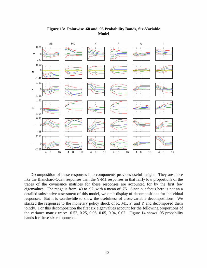
40

Figure 13: Pointwise .68 and .95 Probability Bands, Six-VariableModel

-.64

0

0.71MS

MD

Y

P

U

I

-1.42

0

0.92

-1.15

0

1.11

-1.04

0

1.62

-.45

0

0.42

4 8 16-2.18

0

2.91

4 8 16

4 8 16

4 8 16

4 8 16

4 8 16

Decomposition of these responses into components provides useful insight. They are morelike the Blanchard-Quah responses than the Y-M1 responses in that fairly low proportions of thetraces of the covariance matrices for these responses are accounted for by the first feweigenvalues. The range is from .49 to .97, with a mean of .75. Since our focus here is not an adetailed substantive assessment of this model, we omit display of decompositions for individualresponses. But it is worthwhile to show the usefulness of cross-variable decompositions. Westacked the responses to the monetary policy shock of R, M1, P, and Y and decomposed themjointly. For this decomposition the first six eigenvalues account for the following proportions ofthe variance matrix trace: 0.52, 0.25, 0.06, 0.05, 0.04, 0.02. Figure 14 shows .95 probabilitybands for these six components.

41

Figure 14: Components 1-6 of Joint Response of R, M, P, Y toMonetary Policy, .95 Bands, Six-Variable Model

-.32

0

.401

2

3

4

5

6

-1.29

-.64

0

.48

4 8 16-.84

0.12

4 8 16

4 8 16

4 8 16

4 8 16

4 8 16

The most interesting aspect of this graph emerges only with careful attention to the differentline colors. For the first component, in column 1, the top lines in plots of the responses of M andY match the bottom lines in the plots of responses of R and P. Thus more positive responses ofR and P are associated with more negative responses of M and Y. The first three variables areconsistent in suggesting that the main component of uncertainty is simply the uncertainty aboutthe strength of the effect of the shock – is the increase in R, decline in M, and initial decline in Ylarge, or small? But the P component shows the opposite pattern – large R, M, and Y responsesare associated with weak P responses, and vice versa. This pattern could be relevant tointerpretation of the model’s results, and would be very important to include in characterizationsof uncertainty about conditional forecasts from the model used in policy analysis.

The second column weights most heavily on M and P, indeed is more important for M than isthe first component. Here M and P move together. This component suggests that there issubstantial uncertainty about the general effect on nominal variables of monetary contraction,independent of uncertainty about how strongly monetary contraction affects the interest rate andoutput. The third component affects mostly the output response, the fourth mostly the Mresponse, and the fifth mostly the R response, but all are modest in size.

This model shows only moderate simultaneity, so that difference between these correctlycomputed bands and bands computed by the naive Bayesian method or by using unweighted

42

draws from the asymptotic normal approximation to the p.d.f. for A0 are correspondinglymodest. The bands around responses to monetary policy disturbances are particularly similaracross methods, probably because these responses are relatively sharply determined. Differencesare more clearly visible in the responses to MD and Y shocks, which are more ill-determined. InFigure 15 we compare bands constructed correctly by Metropolis chain, by the naive Bayesianmethod, and by unweighted draws from the Gaussian approximation based on the Hessian of thelog likelihood at the MLE. One response that is of interpretive interest for which bands come outdifferently across these methods is that of R to a Y shock. The Y shock is major source ofvariation in output, and a positive response of R to this shock suggests that monetary policy tendsto tighten when output expands. But note that in Figure 15 the 95% band extends well intonegative range for the initial R-to-Y response, indicating considerable uncertainty about thestrength of this response. The two other methods, by contrast, show 95% bands that in each caseare entirely positive. The responses to MD are of less substantive interest, since the results seemto show that this set of responses is so ill-determined that interpretation is dubious. However, itcan be seen that there is a general tendency for the third and fifth columns, using the naive andunweighted methods, to give narrower bands than the first column Finally, the band for theresponse of price to MD in the third column, corresponding to the naive Bayesian procedure,shows hardly any skewness, while the likelihood in fact shows very strong skewness, with the68% band lying almost entirely below the point estimate.26

26 We are confident that the differences discussed here are not artifacts of Monte Carlo samplingerror. 8000 independent draws were used for the naive Bayesian and unweighted Bayesianbands, allowing quite precise estimates of the positions of bands. For the Metropolis chainestimates in the first two columns, we compared results for the pooled Monte Carlo sample withthose for the three independent chains separately. The differences across the bands from thethree chains were barely detectable by eye, so every pattern we discuss in the text is sharplydetermined.

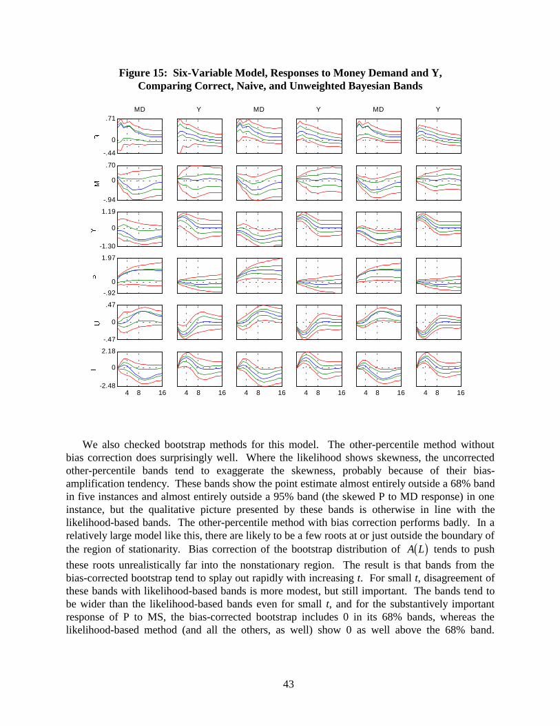
43

Figure 15: Six-Variable Model, Responses to Money Demand and Y,Comparing Correct, Naive, and Unweighted Bayesian Bands

-.44

0

.71MD

Y

MD

Y

MD

Y

-.94

0

.70

-1.30

0

1.19

-.92

0

1.97

-.47

0

.47

4 8 16-2.48

0

2.18

4 8 16

4 8 16

4 8 16

4 8 16

4 8 16

We also checked bootstrap methods for this model. The other-percentile method withoutbias correction does surprisingly well. Where the likelihood shows skewness, the uncorrectedother-percentile bands tend to exaggerate the skewness, probably because of their bias-amplification tendency. These bands show the point estimate almost entirely outside a 68% bandin five instances and almost entirely outside a 95% band (the skewed P to MD response) in oneinstance, but the qualitative picture presented by these bands is otherwise in line with thelikelihood-based bands. The other-percentile method with bias correction performs badly. In arelatively large model like this, there are likely to be a few roots at or just outside the boundary ofthe region of stationarity. Bias correction of the bootstrap distribution of A Lb g tends to push

these roots unrealistically far into the nonstationary region. The result is that bands from thebias-corrected bootstrap tend to splay out rapidly with increasing t. For small t, disagreement ofthese bands with likelihood-based bands is more modest, but still important. The bands tend tobe wider than the likelihood-based bands even for small t, and for the substantively importantresponse of P to MS, the bias-corrected bootstrap includes 0 in its 68% bands, whereas thelikelihood-based method (and all the others, as well) show 0 as well above the 68% band.

44

Conclusions about whether the model shows a “price puzzle” might therefore be distorted by useof bias-corrected bootstrap intervals.

IX. Conclusion

We have explained the reasons for computing likelihood-characterizing error bands indynamic models, shown how to go beyond the standard pointwise bands to display shapeinformation, shown that the methods we propose are computationally feasible, and shown thatother approaches can fall short in characterizing actual likelihoods, even though they are knownto provide accurate approximations in large enough samples. We hope to have convincedapplied researchers that likelihood-characterizing bands are the best approach to providing errorbands in time series models. We hope to have convinced theoretical researchers that improvinglikelihood-based approaches is a more productive use of intellectual effort than further attemptsto provide confidence bands with asymptotic justification.

Department of Economics, Yale University,37 Hillhouse Avenue, New Haven, CT 06520-8264sims@econ.yale.edu; http://www.econ.yale.edu/~sims

andFederal Reserve Bank of Atlanta104 Marietta Street, Atlanta GA 30303tzha@mindspring.com

45

References

Bekker, Paul A. and D.S.G. Pollock (1986): “Identification of Linear Stochastic Models withCovariance Restrictions,” Journal of Econometrics, 31, 179-208.

Berger, James O. and Robert L. Wolpert (1988): The Likelihood Principle (2nd Edition),Hayward, California: Institute of Mathematical Statistics.

Blanchard, O.J. and D. Quah(1989): “The Dynamic Effects of Aggregate Demand and SupplyDisturbances,” American Economic Review, 79, 655-73

Bose, A. (1988): “Edgeworth Correction by Bootstrap in Autoregressions”, Annals of Statistics16, 1709-1722.

Box, G.E.P. and George Tiao (1973): Bayesian Inference in Statistical Analysis. Addison-Wesley.

Canova (1991)Canova, Fabio (1991): “The Sources of Financial Crisis: Pre- and Post-FedEvidence,” International Economic Review, 32, 689-713.

Dufour, J.-M., (1997): “Some impossibility theorems in econometrics with applications tostructural and dynamic models”, Econometrica 65, 1365-1387.

Efron, Bradley and Robert J. Tibshirani (1993): An Introduction to the Bootstrap, New York andLondon: Chapman and Hall.

Faust, Jon (1996). “Near Observational Equivalence and Theoretical Size Problems with UnitRoot Tests," Econometric Theory, 12, pp.724-731.

Ferguson, Thomas S. (1967): Mathematical Statistics: A Decision Theoretic Approach, (NewYork and London: Academic Press).

Geweke, John (1995): “Bayesian Comparison of Econometric Models”, processed, University ofMinnesota.

)Gelman, Andrew, John B. Carlin, Hal S. Stern, and Donald B. Rubin (1995): Bayesian DataAnalysis, London: Chapman and Hall.

Gordon, D.B. and E.M. Leeper (1994): “The Dynamic Impacts of Monetary Policy: An Exercisein Tentative Identification,” Journal of Political Economy , 102, 1228-1247.

Hall, Peter (1992): The Bootstrap and Edgeworth Expansion, Springer-Verlag.

Hildreth, Clifford (1963): “Bayesian Statisticians and Remote Clients,” Econometrica, 31, 422-439.

Horowitz and Savin (1998)Horowitz, Joel L. and N. E. Savin (1998): “Empirically RelevantCritical Values For Hypothesis Tests: The Bootstrap To The Rescue”, processed, Departmentof Economics, University of Iowa.

Kilian, Lutz (1998a): “Small-Sample Confidence Intervals for Impulse Response Functions,”Review of Economics and Statistics, 80, 186-201.

Kilian, Lutz (1998b): “Pitfalls in Constructing Bootstrap Confidence Intervals for AsymptoticallyPivotal Statistics,” processed, Department of Michigan.

46

Kloek, T. and H.K. van Dijk (1978): “Bayesian Estimates of Equation System Parameters: AnApplication of Integration by Monte Carlo,” Econometrica, 46, 1-19.

Koop, G. (1992): “Aggregate Shocks and Macroeconomic Fluctuations: A Bayesian Approach,”Journal of Applied Econometrics, 7, 395-411.

Kwan, Yum K. (1998): “Asymptotic Bayesian Analysis Based on a Limited InformationEstimator”, City University of Hong Kong discussion paper, forthcoming in Journal ofEconometrics.

Lastrapes, W.D. and G. Selgin (1994): “Buffer-Stock Money: Interpreting Short-Run DynamicsUsing Long-Run Restrictions,” Journal of Money, Credit and Banking, 26, 34-54.

Loève, Michel (1988). Comment in Berger and Wolpert (1988).

Lutkepohl, H. (1990): “Asymptotic Distributions of Impulse Response Functions and ForecastError Variance Decompositions of Vector Autoregressive Models,” The Review of Economicsand Statistics, 72, 53-78.

Mittnik, S. and P.A. Zadrozny (1993): “Asymptotic Distributions of Impulse Responses, StepResponses, and Variance Decompositions of Estimated Linear Dynamic Models,”Econometrica, 20, 832-854.

Poterba, J.M., J.J. Rotemberg and L.H. Summers (1986): “A Tax-Based Test for NominalRigidities,” American Economic Review, 76, 659-675.

Phillips, P.C.B. (1992): “To Criticize the Critics: An Objective Bayesian Analysis of StochasticTrends,” Journal of Applied Econometrics, 7.

RATS, computer program available from Estima, 1800 Sherman Ave., Suite 612, Evanston IL60201.

Rothenberg, Thomas J., and James H. Stock (1997): “Inference in a nearly integratedautoregressive model with nonnormal innovations”, Journal of Econometrics 80, 269-286.

Runkle, D.E. (1987): “Vector Autoregressions and Reality,” Journal of Business and EconomicStatistics, 5, 437-442.

Sims, C.A. (1986): “Are Forecasting Models Usable for Policy Analysis?” Federal ReserveBank of Minneapolis Quarterly Review 10, 2-15.

Waggoner, Daniel F. and Tao Zha (1997): “Normalization, Probability Distribution, and ImpulseResponses,” Federal Reserve Bank of Atlanta Working paper 97-11

Waggoner, Daniel F. and Tao Zha (1998): “Identification Issues in Vector Autoregressions,”processed, Federal Reserve Bank of Atlanta.

Wilks, Samuel S. (1962): Mathematical Statistics, New York, London: John Wiley and Sons.

Zacks (1971)Zacks, Shelemyahu: The Theory of Statistical Inference, New York, London,Sydney, Toronto: John Wiley and Sons, 1971.