Essays on

Behavior under Risk and Uncertainty

Inaugural-Dissertation

zur Erlangung des Doktorgrades

der

Wirtschafts- und Sozialwissenschaftlichen Fakultät

der

Universität zu Köln

2012

vorgelegt von

Dipl.-Vw. Julia Stauf

aus

Siegburg

Referent: Prof. Dr. Axel Ockenfels

Korreferent: Prof. Dr. Bernd Irlenbusch

Tag der Promotion: 21. Januar 2013

i

Acknowledgements

The writing of this dissertation has been one of the greatest intellectual and personal challenges

I have faced. It would not have been completed without the support, motivation and guidance of

the following persons.

First and foremost, I thank my supervisor Axel Ockenfels for giving me the opportunity to work

in an excellent academic environment and for guiding my research. His ideas, his knowledge and

his commitment to the highest methodological standards inspired and challenged me and

deepened my understanding of science.

I thank my second supervisor Bernd Irlenbusch for his valuable comments and for reviewing my

thesis.

I thank my co-authors Gary Bolton, Christoph Feldhaus, Diemo Urbig and Utz Weitzel for fruitful

discussions and for close collaboration in our joint research projects.

I thank my present and former colleagues Sabrina Böwe, Olivier Bos, Felix Ebeling, Christoph

Feldhaus, Vitali Gretschko, Lyuba Ilieva, Jos Jansen, Sebastian Lotz, Johannes Mans, Alex Rajko,

Diemo Urbig and Peter Werner for the great working atmosphere, for countless discussions of

academic, general and personal matters, and for making research fun. Beyond this, I thank Vitali

and Alex for repeated corrections of my beliefs about my success probability.

I thank our student helpers and in particular Markus Baumann, Andrea Fix, Gregor Schmitz and

Johannes Wahlig for providing excellent research assistance.

I thank Thorsten Chmura, Sebastian Goerg and Johannes Kaiser for sharing their knowledge with

me during the time I spent with them at the Bonn Laboratory for Experimental Economics, and

especially for encouraging me to pursue a doctoral degree.

I thank Martin Offer for conducting an experiment on me during my diploma studies by

incentivizing the hours I spent in the library. His results were highly significant both in terms of

my interest in the field and my grades.

Finally, I thank my sisters Viola and Leonie Stauf, my brother Patrick Stauf, my mother Hildegard

Hass-Stötzel and my father Franz-Josef Stauf for their support, patience and confidence.

ii

Table of contents

1 Introduction ............................................................................................................................................. 1

2 What is your level of overconfidence? A strictly incentive compatible measurement

method ................................................................................................................................................................. 5

2.1 Introduction ...................................................................................................................................................... 5

2.2 Overconfidence measurements and potential improvements ..................................................... 7

2.2.1 Incentive compatibility ....................................................................................................................... 7

2.2.2 Precision and comparability of confidence measurements ............................................. 10

2.3 Characteristics of the proposed method ............................................................................................ 10

2.3.1 Experimental design ......................................................................................................................... 12

2.3.2 Measurements ..................................................................................................................................... 14

2.3.3 Formal proof of strict incentive compatibility ....................................................................... 15

2.4 Results .............................................................................................................................................................. 19

2.4.1 Simultaneous over- and underconfidence at the population level ................................ 20

2.4.2 Confidence in absolute versus relative performance .......................................................... 21

2.5 Conclusions .................................................................................................................................................... 23

2.6 Appendix ......................................................................................................................................................... 25

3 Risk taking in a social context ......................................................................................................... 34

3.1 Introduction ................................................................................................................................................... 34

3.2 Main experiments ........................................................................................................................................ 35

3.2.1 Experimental design ......................................................................................................................... 35

3.2.2 Procedure .............................................................................................................................................. 38

3.2.3 Results .................................................................................................................................................... 38

3.3 Additional tests ............................................................................................................................................. 42

3.3.1 Experimental design ......................................................................................................................... 42

3.3.2 Procedure .............................................................................................................................................. 43

3.3.3 Results .................................................................................................................................................... 43

3.4 Conclusion ...................................................................................................................................................... 47

3.5 Appendix ......................................................................................................................................................... 48

4 A hero game ........................................................................................................................................... 56

4.1 Introduction ................................................................................................................................................... 56

4.2 The hero game .............................................................................................................................................. 57

4.2.1 Version 1 (a b) ................................................................................................................................ 58

4.2.2 Version 2 (a b) ................................................................................................................................ 59

4.3 Experiment ..................................................................................................................................................... 62

iii

4.3.1 Design ..................................................................................................................................................... 62

4.3.2 Procedure .............................................................................................................................................. 64

4.4 Hypotheses ..................................................................................................................................................... 65

4.5 Results .............................................................................................................................................................. 66

4.5.1 Treatment 1 .......................................................................................................................................... 66

4.5.2 Treatment 2 .......................................................................................................................................... 67

4.5.3 Treatment comparison .................................................................................................................... 69

4.6 Discussion ....................................................................................................................................................... 69

4.7 Conclusion ...................................................................................................................................................... 74

4.8 Appendix ......................................................................................................................................................... 75

5 Speak up, hero! The impact of pre-play communication on volunteering ..................... 78

5.1 Introduction ................................................................................................................................................... 78

5.2 Theory .............................................................................................................................................................. 80

5.2.1 The hero game ..................................................................................................................................... 80

5.2.2 Communication ................................................................................................................................... 83

5.3 Hypotheses ..................................................................................................................................................... 85

5.3.1 One-way communication ................................................................................................................ 85

5.3.2 Multi-way communication ............................................................................................................. 87

5.3.3 Treatment comparison .................................................................................................................... 89

5.4 Experimental design ................................................................................................................................... 90

5.5 Procedure ........................................................................................................................................................ 91

5.6 Results .............................................................................................................................................................. 92

5.6.1 One-way communication ................................................................................................................ 92

5.6.2 Multi-way communication ............................................................................................................. 94

5.6.3 Treatment comparison .................................................................................................................... 95

5.7 Efficiency concerns in the hero game .................................................................................................. 97

5.7.1 One-way communication ................................................................................................................ 99

5.7.2 Multi-way communication .......................................................................................................... 102

5.8 Intermediary signals as coordination device in the multi-way communication

treatment .................................................................................................................................................................... 103

5.8.1 Hypotheses ........................................................................................................................................ 103

5.8.2 Results ................................................................................................................................................. 105

5.9 Conclusion ................................................................................................................................................... 108

5.10 Appendix ...................................................................................................................................................... 109

6 Conclusion ............................................................................................................................................ 119

7 References ............................................................................................................................................ 120

iv

List of tables

Table 1: Descriptive statistics (mean, standard deviation, mode) and selected correlations ........ 19

Table 2: Individual and social risk aversion depending on order .............................................................. 44

Table 3: Individual and social risk aversion with information .................................................................... 44

Table 4: Mean adjustment in direction of matched participant .................................................................. 45

Table 5: Adjustment of risk preferences towards the mean signal in Experiment 7 .......................... 46

Table 6: Payoff table treatment T1 .......................................................................................................................... 63

Table 7: Payoff table treatment T2 .......................................................................................................................... 64

Table 8: Fraction of choices of ....................................................................................................................... 68

Table 9: Conditions, predicted impulses and adjustments ............................................................................ 70

Table 10: Fraction of observations consistent/inconsistent with ex-post rationality ....................... 75

Table 11: Treatment overview .................................................................................................................................. 90

Table 12: Payoff table .................................................................................................................................................... 91

Table 13: Signals and corresponding effort choices ......................................................................................... 93

Table 14: Comparison of effort choices of senders and non-senders ....................................................... 93

Table 15: Mean profits and frequency of perfect coordination conditional on signal ....................... 94

Table 16: Treatment comparison of profits and perfect coordination ..................................................... 96

Table 17: Mapping of signals into effort choices ............................................................................................. 100

Table 18: Signaling strategies and resulting utility for player i with efficiency concerns ............. 102

Table 19: Utilities in the reduced effort stage .................................................................................................. 104

Table 20: Utilities in the reduced two-stage game ......................................................................................... 105

Table 21: Direction of adjustment ........................................................................................................................ 107

Table 22: Mean profits and efforts with multi-way communication ...................................................... 107

Table 23: Profit, signal and deviation from signal (one-way communication) .................................. 109

v

List of figures

Figure 1: Course of the experiment ......................................................................................................................... 13

Figure 2: Population’s better-than-others beliefs ............................................................................................. 21

Figure 3: Comparison of confidence regarding absolute and relative performance .......................... 22

Figure 4: Overview of main experiments .............................................................................................................. 36

Figure 5: Overview experiments 5, 6 and 7 ......................................................................................................... 42

Figure 6: Effort choices across periods (T1) ........................................................................................................ 67

Figure 7: Effort choices across periods (T2) ........................................................................................................ 68

Figure 8: Expected utility of strategies ei = 1,..., 7 .............................................................................................. 73

Figure 9: Distribution of signals within the treatment groups .................................................................... 95

Figure 10: Treatment comparison of mean profits ........................................................................................... 96

Figure 11: Mean efforts conditional on whether the player has sent the unique highest signal 106

Figure 12: Distribution of effort levels and signals (multi-way communication) ............................. 109

1

1 Introduction

One of the core topics in economics is choice behavior under risk and uncertainty: A decision

maker chooses from a set of actions, the outcomes of which depend on the true state of the

world which is a priori unknown to the decision maker. Whereas risk is measurable in the sense

that probabilities for all possible states of the world are given and known, this is not the case for

uncertainty (Knight 1921). An important source of uncertainty is the behavior of others in social

interactions, which is referred to as strategic uncertainty (Van Huyck et al. 1990, Brandenburger

1996). This dissertation comprises four experimental studies that deal with different kinds of

risk and uncertainty, ranging from risk in simple lotteries to strategic uncertainty resulting from

others’ actions.

Actual human choice behavior is often found to diverge from the assumptions of standard

economic theory. The field of behavioral economics augments established economic models by

integrating insights from psychology, thereby increasing their explanatory power (Camerer and

Loewenstein 2004). DellaVigna (2009) defines three kinds of deviations from standard theory

that influence the outcome of decision making processes. First, non-standard preferences imply

that factors apart from the decision maker’s own outcome have an impact on her utility. A

prominent example for non-standard preferences are social preferences, which means that a

decision maker’s utility is influenced by (her beliefs about) the outcome of others. An increasing

number of studies shows the importance of social preferences under certainty;1 yet, little is

known about behavior in a social context under uncertainty. The second and the fourth study in

this thesis deal with the question how social preferences affect decision making under risk and

under strategic uncertainty, respectively.2 Second, non-standard beliefs are characterized by a

systematic bias in the perception of the probabilities associated with different states of the

world. One example of biased beliefs is overconfidence, the systematic overestimation of own

performance, which is dealt with in the first study. Third, non-standard decision-making refers to

1 For an overview see e.g. Fehr and Schmidt (2006). 2 Social preferences are also briefly discussed in the third study.

2

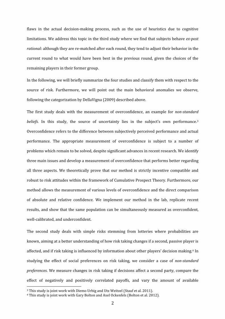
flaws in the actual decision-making process, such as the use of heuristics due to cognitive

limitations. We address this topic in the third study where we find that subjects behave ex-post

rational: although they are re-matched after each round, they tend to adjust their behavior in the

current round to what would have been best in the previous round, given the choices of the

remaining players in their former group.

In the following, we will briefly summarize the four studies and classify them with respect to the

source of risk. Furthermore, we will point out the main behavioral anomalies we observe,

following the categorization by DellaVigna (2009) described above.

The first study deals with the measurement of overconfidence, an example for non-standard

beliefs. In this study, the source of uncertainty lies in the subject’s own performance.3

Overconfidence refers to the difference between subjectively perceived performance and actual

performance. The appropriate measurement of overconfidence is subject to a number of

problems which remain to be solved, despite significant advances in recent research. We identify

three main issues and develop a measurement of overconfidence that performs better regarding

all three aspects. We theoretically prove that our method is strictly incentive compatible and

robust to risk attitudes within the framework of Cumulative Prospect Theory. Furthermore, our

method allows the measurement of various levels of overconfidence and the direct comparison

of absolute and relative confidence. We implement our method in the lab, replicate recent

results, and show that the same population can be simultaneously measured as overconfident,

well-calibrated, and underconfident.

The second study deals with simple risks stemming from lotteries where probabilities are

known, aiming at a better understanding of how risk taking changes if a second, passive player is

affected, and if risk taking is influenced by information about other players’ decision making.4 In

studying the effect of social preferences on risk taking, we consider a case of non-standard

preferences. We measure changes in risk taking if decisions affect a second party, compare the

effect of negatively and positively correlated payoffs, and vary the amount of available

3 This study is joint work with Diemo Urbig and Utz Weitzel (Stauf et al. 2011). 4 This study is joint work with Gary Bolton and Axel Ockenfels (Bolton et al. 2012).

3

information. We find that participants use the available information to adjust their risk taking,

thus behaving more conform with others. Moreover, this adjustment occurs more often and to a

higher degree if this implies less risk taking than before, leading to higher conservatism in a

social context. The more the decisions are embedded in a social context, the more pronounced

are these effects.

The third and the fourth study deal with strategic uncertainty in an n-person hero game.5 We

investigate a situation in which exactly one person within a group should make a costly effort to

increase the payoff of everyone else and reach the socially efficient outcome. In the third study,

we investigate two versions of the hero game that differ with respect to their equilibria; while

the first version of the game offers one equilibrium in dominant strategies in the one-shot game,

the second version is a classical coordination game with n pure strategy equilibria. While

behavior in the first version is largely in line with standard theory, we find that in the

coordination game, a substantial fraction of players chooses strategies that should never be

chosen according to standard theory. We discuss social preferences and risk aversion as

potential explanations for these deviations. Furthermore, we find that players tend to behave ex-

post rational; even if they are randomly rematched, they tend to adjust their behavior to their

experience in the previous round. This behavioral pattern is an example of non-standard decision

making.

In a follow-up study, we focus on the version of the hero game that represents a coordination

problem. Probably the most common means to solve coordination problems is communication

between the involved parties. We investigate the impact of two different communication

mechanisms on coordination. The first mechanism allows one randomly chosen player to send a

message to the other players to indicate which effort she is going to choose, which we refer to as

one-way communication. The second mechanism termed multi-way communication allows all

players to send messages to each other simultaneously. We show that, from a theoretical point of

view, multi-way communication should not have any effect, while one-way communication

5 The third study is joint work with Christoph Feldhaus (Feldhaus and Stauf 2012) and is based on a diploma thesis (Feldhaus 2011).

4

should lead to a substantially higher coordination rate. In particular, we show that there exists

an asymmetric mixed-strategy equilibrium which results in a higher expected overall payoff

than the symmetric one, and we argue that it is plausible that this equilibrium is played with

one-way communication. However, our experimental data shows that multi-way communication

significantly improves coordination in comparison to a situation without communication, while

one-way communication leads to mixed results. We propose non-standard preferences and in

particular efficiency concerns as an explanation for the deviations from standard theory.

I contributed to the respective chapters in the following way. I developed the general idea for the

first paper (Stauf et al. 2011, chapter 2). I designed, programmed and conducted the experiment

in collaboration with Diemo Urbig. I carried out most of the statistical analyses, and I wrote the

major part of the draft. Regarding the second paper (Bolton et al. 2012, chapter 3), I was

centrally involved in the development of the idea and the hypotheses, as well as in the design of

the experiment. I programmed and conducted the experiment, and I carried out the majority of

the statistical analyses. I wrote the draft in collaboration with Gary Bolton and Axel Ockenfels.

The third paper (Feldhaus and Stauf 2012, chapter 4) is based on a diploma thesis written by

Christoph Feldhaus that was supervised by Axel Ockenfels and myself; the idea for this paper

came from Axel Ockenfels. I participated in the development of the hypotheses and the design.

The experiment was programmed and conducted by Christoph Feldhaus. The draft at hand is

based on the text of the diploma thesis; I rewrote substantial parts and added a number of

statistical analyses. The fourth paper (Stauf 2012, chapter 5) was single-authored. I developed

the idea and the hypotheses based on the third paper, and I used parts of the data from the

previous experiments as baseline. I designed, programmed and conducted two additional

treatments, I carried out all statistical analyses, and I wrote the draft.

5

2 What is your level of overconfidence?

A strictly incentive compatible measurement method6

2.1 Introduction

Overconfidence is a frequently observed, real-life phenomenon. Individuals exaggerate the

precision of their knowledge, their chances for success, or the precision of specific types of

information. Empirically, it has been shown that overconfidence in own performance can affect

an entrepreneur's or manager's decision to enter a market (Camerer and Lovallo 1999, Wu and

Knott 2006) or to invest in projects (Malmendier and Tate 2005), a stock trader’s decision to buy

specific stocks (Daniel et al. 1998, Stotz and von Nitzsch 2005, Cheng 2007), or an acquirer’s

decision to take over a target firm (Malmendier and Tate 2008). Lawyers' and applicants'

probabilities of success are likely to depend on confidence (Compte and Postlewaite 2004), and

physicians have been shown to be overconfident in their choices of medical treatment (Baumann

et al. 1991). Especially the last example illustrates that the consequences of overconfidence do

not only affect the decision maker, but can also have significant ramifications for third parties

(e.g., patients, clients, investors, employees), as well as the economy and our society as a whole.

One stream in overconfidence research attempts to identify mechanisms that lead to

overconfidence (e.g. Soll 1996, Juslin and Olsson 1997, Hilton et al. 2011). A second research

stream studies how overconfidence affects evaluations of risky decision options and subsequent

decisions (e.g. Simon et al. 2000, Keh et al. 2002, Cheng 2007, Coelho and de Meza 2012). A

further stream of research, in which our study is embedded, is concerned with the definition and

correct measurement of overconfidence.

In an early study, Fischhoff et al. (1977) consider incentives within overconfidence

measurements as a potential source of measurement errors. Hoelzl and Rustichini (2005) test

the effect of monetary incentives and indeed find significant differences between treatments in

which participants are incentivized and those in which they are not. Despite recent advances, we

6 This study is joint work with Diemo Urbig and Utz Weitzel (Stauf et al. 2011).

6

argue that currently available mechanisms to experimentally elicit individuals’ overconfidence

(e.g. Moore and Healy 2008, Blavatskyy 2009) still allow for improvements in the area of

incentive compatibility and in measuring subjects’ magnitude of overconfidence more precisely.

To address these issues, we present a method of overconfidence elicitation that is strictly

incentive compatible within the framework of rank-dependent utility theories, is robust to risk

attitudes, and identifies different levels of overconfidence. This method does not only improve

existing procedures, but also enables a direct within-subject comparison of absolute

overconfidence (with respect to one’s performance) and relative overconfidence (with respect

to being better than others), as both types are measured with the same methodology.

In experimentally testing this method, we provide first evidence for the importance of

measuring different levels of overconfidence: We find that participants are simultaneously over-

and underconfident at the population level, depending on the thresholds of relative

performance. Although 95 % of participants believe to be better than at least 25 % of the

population (implying overconfidence for low thresholds), only 7 % believe to be among the best

25 % (implying underconfidence for high thresholds). We argue that the application of relative

thresholds that are different from the population median can provide valuable new insights. For

instance, a general underconfidence to be among the best could lead to pessimism in highly

competitive environments such as patent races, where investment in research and development

depends on the firm’s confidence in its relative performance, or takeover auctions, where the

highest bid depends on the acquirer’s confidence in realizing enough synergies to refinance the

deal.

The chapter is organized as follows. The next section discusses existing methods of incentivized

overconfidence elicitation and possible further improvements. In section 2.3, we present an

experimental design for measuring absolute and relative overconfidence, and formally show its

strict incentive compatibility. In section 2.4, we report the experimental results, compare them

with the findings of previously used methods and present the characteristics of the new method.

7

Section 2.5 concludes with a discussion of limitations, future research, and possible implications

of measuring levels of overconfidence.

2.2 Overconfidence measurements and potential improvements

Considering the diverse contexts in which overconfidence has been investigated, it is not

surprising that various definitions of overconfidence have been used (see e.g. Griffin and Varey

1996, Larrick et al. 2007, Moore and Healy 2008, Fellner and Krügel 2011). We adopt the

definition by Griffin and Varey (1996), who specify optimistic overconfidence as overestimating

the likelihood that an individual’s favored outcome will occur. For reasons of legibility, we refer

to optimistic overconfidence simply as overconfidence. We particularly focus on the

overestimation of own performance in a knowledge-based task, which can relate to achieving an

objective standard of performance (absolute overconfidence) or to be better than others

(relative overconfidence).

2.2.1 Incentive compatibility

Already in 1977, Fischhoff et al. raise doubts on whether participants in overconfidence studies

are sufficiently motivated to reveal their true beliefs and therefore introduce monetary stakes.

Hoelzl and Rustichini (2005) report significant differences depending on whether participants

received additional incentives for predicting their performance correctly. While most

overconfidence measurements implicitly assume that participants maximize their performance,

optimizing the predictability by deliberately giving false answers could also be an option,

especially when participants are paid for their precision in prediction. To incentivize

participants to maximize their performance, Budescu et al. (1997) and Moore and Healy (2008)

provide additional monetary payoffs for correctly solved quiz questions. This, however, implies

a tradeoff between maximizing performance and maximizing predictability.

In Budescu et al. (1997) and Moore and Healy (2008), the payoff is calculated by means of the

quadratic scoring rule (Selten 1998), the most widely used instantiation of so called proper

8

scoring rules (Savage 1971).7 However, the proper scoring rules also have some disadvantages.

First, they are rather complex to explain, especially if subjects do not have a sound mathematical

background. Second, proper scoring rules are not robust to variations in risk attitudes (Offerman

et al. 2009). Participants with different risk attitudes will provide different responses even if

they hold the same belief. Recent research on individuals’ beliefs to be better than others has

suggested alternative methods to elicit (relative) overconfidence, some of which can also be

applied to elicit confidence in (absolute) performance. Moore and Kim (2003) provide

participants with a fixed amount of money and allow them to wager any fraction of their

endowment on their performance. While this method has the advantage of avoiding tradeoffs

between maximizing performance and predictability and could be perceived as simpler than

proper scoring rules, it is not robust to risk attitudes either. The more risk averse a participant

is, the less she wagers, which confounds the measurement of the participant’s belief with his or

her risk attitude.

While Moore and Kim’s (2003) investment approach is principally a trade-off between a safe

income and a risky income, Hoelzl and Rustichini (2005) and Blavatskyy (2009) suggest eliciting

overconfidence by implementing a trade-off between the performance risks and a lottery with

predetermined odds. Hoelzl and Rustichini utilize this idea for measuring relative

overconfidence by letting participants choose between playing a fifty-fifty lottery and being paid

if they are better than 50 % of all participants. Blavatskyy measures absolute overconfidence in

answering trivia questions and lets participants choose between being paid according to their

(unknown) performance and playing a lottery. The first option results in a fixed payoff M if a

randomly drawn question has been answered correctly; the second option yields the same

payoff M with a probability that equals the fraction of questions that have been answered

correctly, rendering the expected value of both options equivalent. The third option is to

explicitely state indifference between the first and second option, leading to a random choice

between both. Participants choosing the lottery are considered underconfident; those that

7 Participants receive a fixed amount of money if they perfectly predict the outcome, while the payoff is reduced by the square of the deviation if the prediction is not correct. This provides a strong incentive to come as close as possible to the true value, independent of how certain one is.

9

choose to be paid according to their performance are considered overconfident. If they indicate

indifference between both alternatives, they are considered well-calibrated. This method has

empirically been found to be robust to risk attitudes (Blavatskyy 2009) and, as the method by

Hoelzl and Rustichini, has the elegant feature of incentivized performance maximization and

elicitation of true beliefs at the same time.

The methods of Hoelzl and Rustichini (2005) and Blavatskyy (2009) as well as the revelation

mechanism by Karni (2009) used by Coelho and de Meza (2009) can be considered as instances

of what Offerman et al. (2009) call measuring canonical probabilities, and what Abdellaoui et al.

(2005) label the elicitation of choice-based probabilities. These procedures aim at eliciting an

individual’s belief about the probability of a binary random process with payoffs H and L by

determining a probability for a binary lottery with the same payoffs H and L such that

individuals are indifferent between the random process and the lottery. These methods have

theoretically been shown to be robust to risk attitudes in the framework of Expected Utility

Theory (Wakker 2004), supporting Blavatskyy’s empirical finding. We therefore consider these

methods as an excellent basis for further improvements.

Incentive compatibility in Blavatskyy’s design is based on the assumption of epsilon truthfulness,

which states that participants tell the truth when there is no incentive to lie (Rasmusen 1989,

Cummings et al. 1997). If subjects are well-calibrated and thus indifferent between choosing to

be paid according to their performance and being paid according to a lottery, then Blavatskyy’s

design expects participants to truly and explicitly indicate that indifference. Without the

assumption of epsilon truthfulness, any distribution of overconfident, underconfident, and well-

calibrated measurements could be explained by a population of well-calibrated participants who

choose randomly in case of indifference, leading to a potential understatement of the fraction of

well-calibrated subjects. To circumvent this problem, we propose an experimental design that is

strictly incentive-compatible without the assumption of epsilon truthfulness.

10

2.2.2 Precision and comparability of confidence measurements

The methods suggested by Hoelzl and Rustichini (2005) and Blavatskyy (2009) only reveal

whether or not a belief exceeds a certain threshold. Hoelzl and Rustichini (2005) can show that a

participant believes to be worse or better than 50 % of all participants, but not whether she

believes to be better than any other percentage. In Blavatskyy (2009), subjects are classified as

overconfident, underconfident, or well-calibrated, but it is not possible to state whether one is

more or less overconfident than another within the categories. Hoelzl and Rustichini consider a

population as overconfident if more than 50 % believe to be better than 50 %. We argue that this

classification does not necessarily generalize to other levels of performance. In the following, we

discuss an experimental design that allows us to plot a total of ten levels of a population’s

relative confidence in a range from 5 to 95 % to investigate this proposition.

In addition to measuring overconfidence and underconfidence at more levels, the method also

allows a direct comparison between absolute and relative overconfidence by measuring both

with the same method. This enables new empirical tests in an ongoing theoretical debate. Moore

and Healy (2008) propose a theory based on Bayesian updating that explains why individuals

who are overconfident also believe that they perform below average, and those who are

underconfident believe that they perform above average. Larrick et al. (2007) argue that relative

and absolute confidence, both being part of corresponding overconfidence measures, essentially

represent subjective ability as a common underlying factor. Our experimental test thus

represents a first step toward such a comparison of absolute and relative confidence.

2.3 Characteristics of the proposed method

In an attempt to improve the measurement of overconfidence along the lines discussed above

and building on the methods by Hoelzl and Rustichini (2005) and Blavatskyy (2009), we

propose a method that elicits canonical probabilities based on binary choices. Subjects choose

repeatedly between being paid according to own performance (success or failure) and

participating in a lottery with a given winning probability.

11

By selecting an appropriate set of choices, that is, levels of winning probabilities for the lotteries,

our measurement method classifies participants as well-calibrated if their confidence level is

closer to the actually realized performance than to any other possible performance level.

Thereby, we remove the need for well-calibrated participants to explicitly indicate their

indifference. Furthermore, it provides a more robust strategy for identifying well-calibrated

people in conditions where the realized performance is subject to randomness.

Assume that a participant is well-calibrated, which means that her confidence is equal to the

expected performance. As long as the tasks involve a stochastic component, i.e. include imperfect

knowledge, the realized performance is a random variable represented by a distribution with a

mean mirroring the expected performance of a person. The values that the realized performance

can take are determined by the number of tasks solved. If performance is drawn from a

continuous distribution, then the probability that a participant's true expected performance

matches the realized performance approaches zero. Thus, a well-calibrated participant will not

be classified as such.

Furthermore, we suggest to measure performance and confidence with the same level of

precision. Coelho and de Meza (2012) measure forecasting errors in subjectively expected

probability to complete a skill-based task. While ten levels of confidence are elicited, the

performance measure can only take the values 0 or 1, since there is only one task to be solved.

Subjects are considered optimistic if confidence exceeds realized performance. We argue,

however, that if expected performance is smaller than or equal to 0.5, the closest possible

realization is 0; therefore, a subject who does not succeed in the task is well-calibrated for any

confidence in own performance smaller than or equal to 0.5. A more accurate classification can

be achieved by increasing the number of tasks and, thereby, the number of potential realizations

of performance.

To elicit degrees of overconfidence, we ask participants for multiple binary choices, one of which

is randomly selected to determine the payoff (random lottery design). This method can be

applied to various definitions of performance. We exemplify this by eliciting performance beliefs

12

with respect to two different types of performance, absolute and relative. Both are based on

participants’ answers to ten quiz questions with an equivalent level of difficulty. For absolute

performance, a participant succeeds if she answered one particular quiz question correctly and

fails otherwise. This question is determined randomly. For relative performance, a participant

succeeds if she answered more questions correctly than another randomly assigned participant

who answered the same questions and fails if she answered fewer questions.8 If both answered

the same number of questions correctly, one is randomly considered to have succeeded and the

other to have failed.

2.3.1 Experimental design

The experiment consists of four stages. The instructions can be found in Appendix A. Before

starting the experiment, subjects had to pass a test for understanding the instructions. Figure 1

illustrates the course of the experiment.

Stage 1: Solving quiz questions: As usual in overconfidence experiments, participants solve ten

quiz questions without feedback. For this experiment, we used multiple choice questions with

four possible answers. To ensure a homogeneous level of difficulty, we started with a larger set

of questions used by Eberlein et al. (2006) and selected those questions that were correctly

answered by 40 to 50 % of the participants. This resulted in 28 questions, of which we then

randomly selected ten questions for sessions of our experiment (question list in Appendix C).

Stage 2: Select card stack and relevant quiz question: The experimenter presents 10 stacks of 20

cards each, containing 1, 3, 5, ..., 17, 19 cards with a green cross (wins) and a complementary

number of white cards (blanks).9 Participants do not see the number of cards with green crosses

(henceforth, ‘green cards’) and do not (yet) know the distribution of green cards. One participant

8 We do not directly translate the absolute performance measurement into the relative measurement, because this requires participants to elicit their belief about the probability that they have a higher probability to be correct compared to other participants, which is rather complicated to communicate. We therefore ask them to compare the number of correct questions. As the number of correct questions is the best estimate of the probability to be correct, the direct and the indirect measure we use for the absolute and relative performance are, in fact, equivalent. 9 Note that for the method to be incentive-compatible, it is necessary to ensure that the lowest winning probability of the random mechanism (here: 5 %) is strictly lower than the minimum success probability in the task (here: 25 %). See p. 20 for a detailed explanation.

13

randomly chooses one stack; all other stacks are removed. The same procedure is repeated for a

second set of stacks. Finally, one participant draws one card out of a third stack of 10 (numbered

from 1 to 10) that determines the question that counts for the absolute performances of all

participants.

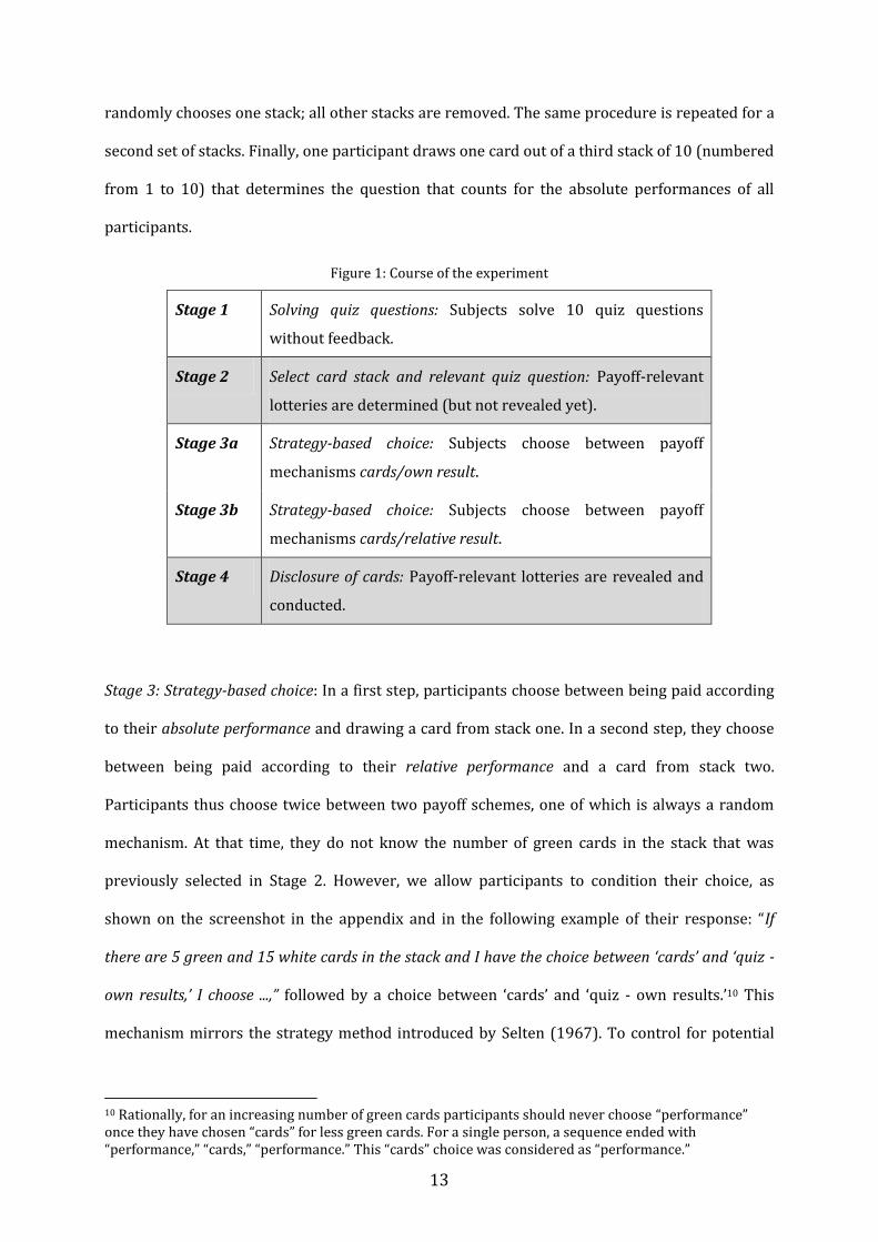
Figure 1: Course of the experiment

Stage 1 Solving quiz questions: Subjects solve 10 quiz questions

without feedback.

Stage 2 Select card stack and relevant quiz question: Payoff-relevant

lotteries are determined (but not revealed yet).

Stage 3a Strategy-based choice: Subjects choose between payoff

mechanisms cards/own result.

Stage 3b Strategy-based choice: Subjects choose between payoff

mechanisms cards/relative result.

Stage 4 Disclosure of cards: Payoff-relevant lotteries are revealed and

conducted.

Stage 3: Strategy-based choice: In a first step, participants choose between being paid according

to their absolute performance and drawing a card from stack one. In a second step, they choose

between being paid according to their relative performance and a card from stack two.

Participants thus choose twice between two payoff schemes, one of which is always a random

mechanism. At that time, they do not know the number of green cards in the stack that was

previously selected in Stage 2. However, we allow participants to condition their choice, as

shown on the screenshot in the appendix and in the following example of their response: “If

there are 5 green and 15 white cards in the stack and I have the choice between ‘cards’ and ‘quiz -

own results,’ I choose ...,” followed by a choice between ‘cards’ and ‘quiz - own results.’10 This

mechanism mirrors the strategy method introduced by Selten (1967). To control for potential

10 Rationally, for an increasing number of green cards participants should never choose “performance” once they have chosen “cards” for less green cards. For a single person, a sequence ended with “performance,” “cards,” “performance.” This “cards” choice was considered as “performance.”

14

order effects, one half of the participants complete the two steps in reverse order, i.e., relative

performance first and absolute performance second.

Stage 4: Disclosure of cards and application of participants’ strategies: In a last step, the number

of green cards in the two stacks and the number of the relevant question are disclosed.

Participants who chose to draw a card from any of the two stacks can individually draw a card.

Payoffs are calculated and individually paid to participants.

2.3.2 Measurements

Our experimental design provides us with the following individual measurements:

Absolute performance p equals the fraction of correctly answered questions.

Relative performance rp is defined as 1 if one participant was better than the other randomly

assigned participant, 0 if she was worse, and 0.5 if she solved as many question as the other.

Confidence c in own absolute performance is the mean of both the highest probability for cards

for which a participant would choose the absolute performance-based payoff rule and the lowest

probability for cards for which a participant would choose the draw of a card from the stack of

cards.

Relative confidence rc in relative performance is the mean of both the highest probability for

which a participant would choose the relative performance-based payoff rule and the lowest

probability for which a participant would choose the draw of a card from the stack of cards.

Absolute overconfidence oc is the difference between absolute confidence and absolute

performance, oc = c - p. We consider participants as well-calibrated when overconfidence oc

equals zero. Note that c is an approximation of a participant’s confidence, and the exact value of

participants confidence lies in the closed interval between c=-0.05 and c=+0.05. As shown below,

participants are well-calibrated when their confidence is closer to their performance than to any

other possible performance.

Relative overconfidence roc is computed analogously to oc: roc = rc - p.

15

2.3.3 Formal proof of strict incentive compatibility

Applied to belief elicitation methods, incentive compatibility describes the fact that a participant

is confronted with incentives that make her reveal her true belief. Strict incentive compatibility

implies that revealing the truth is always strictly preferred such that any deviation results in

lowering the overall value associated with an individual’s decisions. In contrast, weak incentive

compatibility implies that she cannot improve her situation by not revealing the truth

(Rasmusen 1989). Thus, asking individuals for their beliefs without providing any incentives

against lying is weakly, but not strictly incentive compatible.

Before we report the results of the experimental test, we formally show that the proposed

method is strictly incentive compatible and that it has the following properties. First,

participants prefer a higher performance over a lower one, that is, they maximize their

performance. Second, participants choose the lottery if the winning probability of the lottery is

at least as high as their believed performance. Third, a participant is considered well-calibrated

if her performance expectation is closer to the actually realized performance than to any other

possible performance. This third property improves the robustness of classification of people as

well-calibrated. Fourth, elicited probability judgments and resulting classification as

overconfident, underconfident, or well-calibrated are theoretically robust to risk attitudes.

In order to formally show the incentive compatibility, it is necessary to make assumptions about

the participants’ behavior in the form of a descriptive decision theory. For the sake of generality,

we apply the cumulative prospect theory (CPT) by Tversky and Kahneman (1992), although the

following proof also holds for standard expected utility theory.11 Since CPT does not explicitly

consider compound lotteries, i.e., lotteries over lotteries (used in our experiment), we need to

include the reduction axiom as an additional assumption, which states that participants can

reduce compound lotteries to their simple representation.12

11 See p. 21 for a detailed explanation. 12 This axiom has been challenged with respect to its empirical justification, particularly in connection with the use of random lottery mechanisms. However, empirical studies conclude that “experimenters can

16

The proof will be applied to the specific design we use in our experiment, including the double

elicitation of (absolute) confidence and relative confidence. With marginal adjustments, the

proof also holds if the two types of confidence are considered individually.

Participants are confronted with N choices for each of the two elicited confidences; N determines

the precision. In our specific case, N equals 10. Without loss of generality, let ca,i with

1≤i≤N be the participant’s choice between being paid according to own performance and the

lottery i with winning probability pLi . In our case, the lottery i is characterized by 2i-1 winning

cards among the total of 2N cards (in our case, it is 20 cards); thus, pLI=(i-0.5)/N. If the task is

chosen (and not the lottery), ca,i equals 1, otherwise 0. Let cr,i be the same for the choices

between relative performance and a lottery. Vectors ca = ( ca,1, ca,2,… , ca,N) and cr = ( cr,1, cr,2,… , cr,N)

represent vectors of these decisions. Furthermore, let q be the performance expectation by the

participant. Let us assume that the ex-ante performance of the participant varies between qmin

and qmax, i.e qmin ≤ q ≤ qmax (depending on the participant’s choice and ability to influence the own

performance). Let us further assume that the expectation of the relative performance rq is a

strictly monotonic function of the performance expectation, that is, the first derivative of rq’(q)

is strictly larger than 0. Let H be the amount of money that can be won in the lottery or earned

when the task (absolute or relative) has been performed successfully. If the lottery is lost or the

task has not been performed successfully, then participants earn nothing. As participants are

assumed to follow cumulative prospect theory, the preference value V for a given set of decisions

(ca, cr, q) is given by (1), with p being the belief about the occurrence of payoff H. The function

v(x) represents the CPT value function applied to payoffs with v(0) = 0. For simplicity, we also

assume that v(x) > 0 for x > 0. The function (p) represents the CPT probability weighting

function with (p)[0,1]. Both functions are assumed to be monotonically increasing in the

payoff x and the probability p, respectively.

(1)

continue to use the random-lottery incentive mechanism” (Hey and Lee 2005, p. 263). Their results are supported by several other studies, for instance Starmer and Sugden (1991) and Lee (2008).

17

Applying the reduction axiom, a participant is assumed to form a belief about the occurrence of

H depending on her decisions, and she is able to reduce compound lotteries to their simple

representation. This is necessary as our method implements a random choice between

alternatives that are themselves uncertain. Since each of the 2N (in our case 20) choices between

the absolute respectively relative performance and a lottery can become relevant with equal

probability, the probability for H is the average of the probabilities of all single decisions (ca,1 to

ca,N and cr,1 to cr,N). As shown in Equation (2), for a single decision (between absolute

performance and lottery with winning probability pLi) the probability is determined by ca,i q + (1-

ca,i) pLi, which is q if the performance is chosen and pLi if the lottery is chosen. For the choice

between relative performance and a lottery, the probability of a payoff H is determined

correspondingly.

(2)

Note that V(ca,cr,q,H) is always larger than or equal to zero. Equation 2 can be simplified to

with

with the following derivatives with respect to the decision variables:

The terms v(H) and ’(p) are by definition strictly positive. Given that rq’(q) is strictly larger and

c1i and c2i are never less than 0, we can conclude that the preference value is strictly increasing in

q as long as at least one decision is made in favor of being paid according to own absolute or

18

relative performance, i.e., at least one ca,i or cr,i equals 1. In our mechanism, this is the case if the

belief about own performance or the belief about relative performance is greater than 5 %.

Below this threshold, being paid according to own absolute or relative performance is never

chosen, and thus there is no strict incentive to maximize this performance, i.e., the first

derivative is zero. However, the minimal expected probability of success with respect to

absolute performance in our experiment is 25 % (random choice out of four answers per

question) such that the belief about own performance always lies above 5 %. Hence, a

participant always maximizes her performance expectation.13

Furthermore, the preference value is strictly increasing in the decisions cx,i for x being a or r, if q

respectively rq(q) are greater than the winning probability of the alternative lottery. Thus,

participants will always choose the task if their belief to have succeeded is greater than the

probability to win the lottery. Participants therefore always reveal their true beliefs through

their choice behavior. If they do not choose the lottery for lottery i but for i+1, then the best

estimation of the participant’s belief is (pLi + pLi+1)/2, which in our case is i/N.

Note that participants with a confidence between i/N-0.05 and i/N+0.05 are all classified to have

a confidence level of i/N. Such participants are considered well-calibrated if they have solved i

out of N tasks correctly. Therefore, even if their confidence level differs only slightly from the

elicited performance, they will still be classified as well-calibrated. This holds as long as the

difference between confidence and actual performance does not exceed 1/2N, which is

equivalent to the condition that confidence is closer to a different level of performance that

could be elicited.

All results above are based on CPT and the reduction axiom. As such, they are independent of an

individual’s risk attitude as long as it satisfies the axioms of CPT. Our results are thus

theoretically robust to variations in risk attitudes, modeled via value and probability weighting

functions with characteristics following CPT.

13 Note that when excluding the elicitation of confidence in absolute performance such a lower threshold for performance expectations is not present.

19

The proof also holds for expected utility theory (EUT). We assume that the CPT probability

weighting function (p) is monotonically increasing in p, which includes (p) = p, i.e. the absence

of probability weighting. Along the same lines, any strictly increasing utility function u(x) can be

linearly transformed to satisfy the assumptions imposed on the value function v(x).

2.4 Results

We conducted the experiment in two sessions with 31 female and 29 male students from

University of Jena, Germany. We recruited students from all disciplines, ranging from the Natural

to the Social Sciences, with the exception of Psychology. On average, the experimental session

lasted 60 minutes, and participants earned 11.10 Euro.

Table 1: Descriptive statistics (mean, standard deviation, mode) and selected correlations

Descriptive statistics Correlations median p c rc

Performance p 0.497 0.181 0.5 - 0.472 0.475 Relative performance rp 0.500 0.441 0.5 0.551 0.491 0.388 Confidence c 0.492 0.172 0.5 0.472 - 0.728 Relative confidence rc 0.498 0.173 0.5 0.475 0.728 - Overconfidence oc -0.005 0.182 0.00 -0.551 0.476 0.215 Relative overconfidence roc14 -0.002 0.407 0.05 -0.395 -0.223 0.005

Sample size n=60

Table 1 provides some summary statistics for our experiment. The average absolute

performance p is 0.497 with a median of 0.5. On average, participants have a confidence in their

performance of 0.493 with median 0.5 and a confidence in their relative performance of 0.498

with a median 0.5.15 In this experiment, the participants are thus, on average, well-calibrated in

absolute and in relative terms. On an individual basis, we find that 23 % of the subjects are well-

calibrated, while 40 % are underconfident and 37 % are overconfident. The fraction of well-

calibrated subjects is significantly higher in our setting than in Blavatskyy’s (2009) study, a fact

that we ascribe to our avoidance of epsilon-truthfulness as well as applying a more robust

14

There are 30 cases with roc less than or equal to 0.00 and 30 cases greater than or equal to 0.10; thus, 0.05 is by definition the median, despite the fact that this value could not be chosen. 15 One participant violated the basic principle that the probability to win in a multiple choice task with four alternatives is at least 25% if an individual tries to maximize her performance. The behavior of this person who switched between 5% and 15% is not captured by the theories applied here. Since results do not change qualitatively, we kept this data point in the data set.

20

strategy for identifying well-calibrated participants as discussed above.16 We did not find any

order effects; the order of elicitation of absolute and relative confidence did not cause significant

differences.

Table 1 also reports the correlation of variables with performance p, and with confidence

regarding absolute and relative performance. We find that (absolute) performance and relative

performance are positively correlated, as intuitively expected, because participants with a

higher performance have a greater chance to be better than others. Participants are partially

aware of their performance as their (absolute) confidence and relative confidence in their

performance increases with their performance (Pearson correlations are significant at the 5 %

level). However, (absolute) overconfidence and relative overconfidence in performance both

decrease with the level of their performance.17 This result is consistent with prior findings in

overconfidence studies. Moore and Healy (2008) argue that, with higher performance,

participants tend to become less overconfident and even underconfident, but at the same time

believe to be better than others. While the theory by Moore and Healy tentatively suggests a

negative correlation between relative confidence rc and overconfidence oc, we find a positive

relation in our data.

2.4.1 Simultaneous over- and underconfidence at the population level

Above we argued for a more precise measurement of several levels of over- and

underconfidence, instead of focusing on a binary belief to be better or worse than the average of

a population, because an optimistic better-than-average belief may not generalize to an

optimistic better-than-top 5 % belief.

Figure 2 addresses this question by plotting the relative frequency of participants who believe to

be better than 5, 15, 25, …, and 95 %. Consistent with our conclusion from considering the

16 Based on a Chi-square test, we find that the two binary distributions of well-calibrated versus not well-calibrated participants are significantly different at the five percent level. 17 To better understand the relation between correlations involving overconfidence oc=c-p and relative overconfidence roc=rc-rp, on one side, and statistics about the constituent terms, c, rc, p, and rp, on the other, we refer the reader to Appendix A in Larrick et al. (2007), which provides a formal analysis of correlations with one variable being used to calculate the second variable in that correlation.

21

population average of relative confidence, approximately 50 % believe to be better than 50 % of

all participants.

Figure 2: Population’s better-than-others beliefs

Thus, regarding this benchmark the group of our participants is neither over- nor

underconfident. However, considering other benchmarks, the conclusion differs. About 95 % of

all participants believe not to be among the worst 25 %, implying overconfidence; but only about

7 % believe to be among the best 25 %, implying underconfidence. Our group of participants is

therefore underconfident for high and overconfident for low thresholds.

2.4.2 Confidence in absolute versus relative performance

In our experiment, we used the same methodology to elicit confidence in own absolute

performance (confidence) and confidence in own relative performance (relative confidence) at

the same time. This enables a direct comparison of the two types of confidence. A correlation of

0.728 (see Table 1) already indicates that both are closely related. Figure 3 visualizes the

relation between both variables. Besides plotting the data points, it provides conditional means

and a fitted linear approximation of the relation between both variables. As both are subject to

measurement errors, conditional means as well as simple regression analysis yield biased

0

0.2

0.4

0.6

0.8

1

0 0.2 0.4 0.6 0.8 1

Performance threshold t

Rela

tive fre

quency o

f c>

t

Well-calibrated

Underconfidence

Overconfidence

22

results; especially the slope of the fitted linear function might be attenuated.18 However, running

a direct regression (Variable 1 on Variable 2) and a reverse regression (Variable 2 on Variable

1), as illustrated in Figure 3, provides bounds on the true parameter (Wansbeek and Meijer

2000). Despite one outlier with little relative confidence but more or less average (absolute)

confidence, Figure 3 shows an interesting relation between confidence and relative confidence.

In fact, we cannot reject the hypothesis that both are identical for our data. Although this

identity might not be observed in experiments where the average performance is not 50 %, we

would nevertheless expect a close relation of both constructs, albeit at a different level.

Figure 3: Comparison of confidence regarding absolute and relative performance (including conditional means and linear regressions)19

18 For an in-depth discussion of the consequences of measurement errors for overconfidence research, see Erev et al. (1994), Soll (1996), Pfeifer (1994), Brenner et al. (1996), and Juslin et al. (2000). 19 To improve the visibility of data points, we added some small white noise to single data points (but not to the data used for conditional means and regressions).

0

0.2

0.4

0.6

0.8

1

0 0.2 0.4 0.6 0.8 1

Confidence c

Re

lative

co

nfid

en

ce

rc

conditional mean rc | c

conditional mean c | rc

linear regression rc(c)

linear regression c(rc)

23

2.5 Conclusions

This study has been motivated by the ongoing discussion about the appropriate measurement of

overconfidence and, in particular, how to elicit overconfidence in strictly incentive compatible

experiments. We propose and test an experimental design that adapts the advantages of the

existing mechanisms, but adds several desirable features. We show that it is strictly incentive

compatible within the framework of CPT (including EUT), identifies those participants as well-

calibrated whose confidence is closer to their actual performance than to any other possible

performance, is suited to measure overconfidence at more than a maximum of three levels

(overconfidence, underconfidence, and well-calibrated confidence), and can be used to measure

and compare both absolute and relative confidence.

It should be noted that the precision of performance elicitation is driven by the parameter N

describing the number of binary choices used to elicit confidence beliefs. Increasing N also

increases the precision of both confidence and performance measurements, which subsequently

decreases the probability to identify a well-calibrated participant as such. We therefore

recommend analyzing overconfidence with a range of degrees of confidence instead of

dichotomous or trichotomous classifications based on single thresholds. This dependency on

precision also needs to be considered when comparing results of different studies.

A general limitation concerns the common assumption that risk attitudes are independent of the

source of risk. Empirical work seems to suggest that risk attitudes differ for both sources of risk,

own performance, and lotteries (Heath and Tversky 1991, Kilka and Weber 2001, Abdellaoui et

al. 2011). This issue clearly calls for more research into belief elicitation under conditions of

source-dependent risk attitudes.

Besides the methodological advance, this paper also provides applied results. Research on

relative overconfidence generally focuses on the belief to be better than the average of a

population. We argue that for many social and economic situations the belief to be better than

average is of less relevance than the belief to be the best or among the best. Since our

mechanism elicits degrees of overconfidence, we can test whether, for instance, more than 10 %

24

of participants believe to be better than 90 %. In fact, our analysis (visualized in Figure 2) shows

that, simultaneously, too few participants believe to be among the best while too many believe

not to be among the worst. This may have significant economic implications, which would be

worthwhile to investigate in more depth.

25

2.6 Appendix

A: Instructions for participants

There were two versions of the instructions. Both versions differ with respect to the order of

treatments. In the version reported below, the first set of decisions is related to own performance

while the second set of decisions is related to own relative performance. In the second, unreported

version, the order is reversed.

Welcome to our experiment!

General information

You will be participating in an experiment in the economics of decision making in which you can

earn money. The amount of money you will receive depends on your general knowledge and on

your decisions during the experiment. Irrespective of the result of the experiment, you will

receive a show-up fee of €2.50. Please do not communicate with other participants from now on.

If you have any questions, please refer to the experimenters. All decisions are made

anonymously.

You will now receive detailed instructions regarding the course of the experiment.

It is crucial for the success of our study that you fully understand the instructions. After having

read them, you will therefore have to answer a number of test questions to control whether you

understood them correctly. The experiment will not start until all participants have answered

the test questions.

Please read the instructions carefully and do not hesitate to contact the experimenters if you

have any questions.

26

Course of the experiment

After all participants have read the instructions and answered the test questions, we will begin

with the first part of the experiment.

In this part, you will see a sequence of 10 questions, for each of which you will have to choose 1

out of 4 possible answers. One other player in this room will be randomly assigned to you and

will have to solve exactly the same series of questions.

In (the following) parts 2 and 3, we will offer you the opportunity to choose a payoff mechanism.

A payoff mechanism is a method that describes how your payoff will be determined. In both

parts, 2 and 3, you will have to choose between two Options: cards or quiz.

1. Cards

For this mechanism, 20 playing cards will be shuffled. A certain number of these cards bear a

green cross. You will draw one card from the stack. If it bears a green cross, you receive €7. If it

does not bear a green cross, you receive €0. By the time you have to decide for or against this

payoff mechanism, you will know exactly how many of the cards in the stack bear a green cross.

2. Quiz

If you choose this mechanism, your payoff depends on your answers to the quiz questions. The

more questions you have answered correctly, the higher is your chance of receiving a payoff of

€7. There are two variants of the payoff mechanism “quiz”: own result and relative result.

Own result: One out of the 10 quiz questions will be drawn randomly. If you answered this

question correctly, you receive a payoff of €7. Otherwise, you receive €0. With this payoff

mechanism, your payoff will only depend on your own performance.

Relative result: If you answered more questions correctly than the player that has been assigned

to you in the beginning and had to answer exactly the same questions, you receive €7. If you

answered fewer questions correctly, you receive €0. In case of a draw, it will be randomly

decided who receives the €7.

27

In the second part of the experiment, you will be able to choose between the payoff mechanisms

(1) cards or

(2a) quiz – own result.

In the third part of the experiment, you will be able to choose between the payoff mechanisms

(1) cards or

(2b) quiz – relative result.

In both parts, one of your options will be to draw a card from a stack which might bear a green

cross, which is a pure random mechanism. The other option will always be a payoff mechanism,

which determines your payoff based on your result from answering the quiz questions. This

means that, in any case, you should try to correctly answer as many questions as possible. It may

happen that the number of cards with a green cross is always so small that you may prefer to be

paid according to your answers. In this case, your chances are better the more questions you

answered correctly.

The diagram below shows the course of the experiment schematically:

Part 1 Answer quiz questions

Part 2 Choose a payoff mechanism

(1) Cards

or

One out of 20 cards is drawn

Green cross: €7

No green cross: €0

(2a) Quiz – own result

One quiz question is randomly drawn

Correct answer: €7

Wrong answer: €0

Part 3 Choose a payoff mechanism

(1) Cards

or

One out of 20 cards is drawn

Green cross: €7

No green cross: €0

(2b) Quiz –relative result

Another player has been randomly assigned to you.

You answered more questions correctly than him/her: €7

You answered fewer questions correctly than him/ her: €0

28

If you have understood the course of the experiment, you may now start to answer the test

questions you see on your computer screen. You may always, before and during the experiment,

refer to these instructions. The sole aim of the test questions is to control whether you

understood the instructions. They are not the quiz questions you will see in part 1 of the

experiment! The experiment will start when all participants have answered the test questions

correctly.

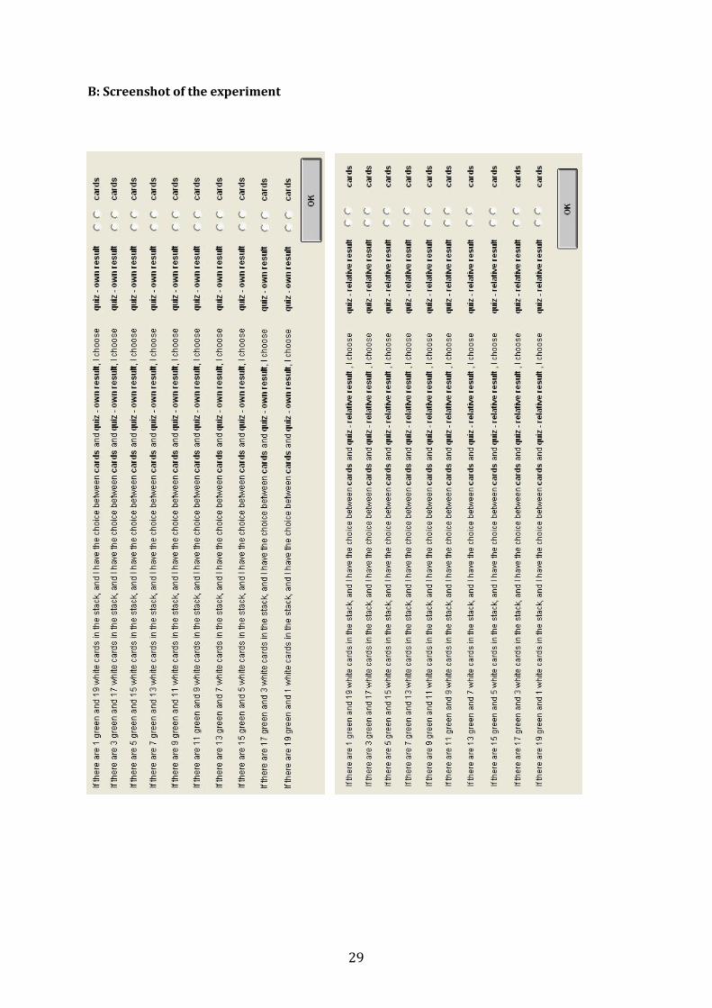
29

B: Screenshot of the experiment

30

C: Quiz questions (translation from German)

1. Which is the first drama written by Friedrich v. Schiller (1759-1805)?

a) Intrigue and Love b) The Robbers c) William Tell d) Fiesco’s Conspiracy at Genoa

2. How many chromosomes does a human cell have?

a) 32 b) 58 c) 46 d) 38

3. A circle with a radius of 2 cm has an approximate circumference of

a) 39.43 cm b) 25.13 cm c) 12.57 cm d) 6.28 cm

4. During which period did the GDR exist?

a) 1945-1989 b) 1950-1990 c) 1948-1989 d) 1949-1990

5. What is the capital of Brazil?

a) Brasilia b) Montevideo c) Buenos Aires d) Rio de Janeiro

6. Which discipline is not part of the heptathlon?

a) Shotput b) Javelin c) Discus d) High jump

7. How large is the third interior angle of a triangle, if the other two angles are 55 degrees and 110 degrees?

a) 195 degrees b) 175 degrees c) 25 degrees d) 15 degrees

8. Which of these countries has the longest coastline?

a) Italy b) France c) Norway d) Spain

31

9. Who wrote Antigone?

a) Sophokles b) Goethe c) Schiller d) Euripides

10. What is the approximate circumference of the earth at the equator?

a) ca. 40 000 km b) ca. 24 000 km c) ca. 36 000 km d) ca. 52 000 km

11. Ozone consists of…

a) Three oxygen atoms b) One carbon atom and two oxygen atoms c) Two oxygen atoms d) One carbon atom and three oxygen atoms

12. Huguenots are …

a) French Jesuits b) French Catholics c) French Jews d) French Calvinists

13. How many articles constitute the civil rights of the German constitution?

a) 9 b) 19 c) 29 d) 39

14. Which animal’s natural habitat is not in the Arctic?

a) Polar bear b) Musk ox c) Penguin d) White fox

15. What is the typical First World War military tactic called?

a) Blitzkrieg b) Guerrilla war c) War of attrition d) Cold War

16. How old is the earth according to current knowledge?

a) ca. 55 billion years b) ca. 5 billion years c) ca. 750 million years d) ca. 25 million years

17. The repetition of the same words or parts of sentences at the beginning of a sentence or verse is known as:

a) Alliteration b) Parallelism c) Anaphora d) Epigram

32

18. How many symphonies did Ludwig van Beethoven compose?

a) 9 b) 15 c) 41 d) 104

19. Which of the following animals is known from modern physics?

a) Teller's dog b) Schrödinger's cat c) Einstein's donkey d) Planck's rabbit

20. Who wrote the book on which the movie "The Silence of the Lambs” is based?

a) Thomas Harris b) Stephen King c) Alfred Hitchcock d) Michael Crichton

21. How big is the surface of a cube with a side length of 3?

a) 18 b) 27 c) 36 d) 54

22. Which of the following animals is not usually found in Asia?

a) Elephant b) Jaguar c) Camel d) Tiger

23. Where does the International Date Line lie?

a) It runs through Greenwich b) It follows the meridian of 180° longitude c) It follows the meridian of 0° longitude d) It runs along the tropic

24. What are the dark spots of the moon called?

a) Mare b) Myra c) Mero d) Mure

25. When did the first Tour de France take place?

a) 1903 b) 1898 c) 1915 d) 1938

26. Which one of these substances is not a metal?

a) Krypton b) Cobalt c) Strontium d) Rubidium

33

27. The length of the diagonal of a rectangle with the side lengths 3 and 4 is

a) 5 b) 7 c) 12 d) 25

28. What is the Shariah?

a) The clothing of an Iman b) The religious law of the Islam c) The headdress of muslimic women d) Islamic celebration at the end of Ramadan

34

3 Risk taking in a social context20

3.1 Introduction

In social contexts without uncertainty, many people care about the fairness of payoff allocations

(Cooper and Kagel forthcoming). Much less is known about social contexts with uncertainty.

Some studies found that social preferences have a much less pronounced effect under

uncertainty than under certainty. Güth et al. (2008), for instance, let subjects evaluate prospects

which allocate payoffs to the subject and a passive participant. They vary whether payoffs are

safe or risky, and whether they are immediate or delayed. Their subjects exhibit other-regarding

preferences only if their own payoff is safe and immediate. Güth et al. conclude that subjects’

other-regarding concerns are crowded out if their own payoff is risky or delayed, and speculate

that this is due to a cognitive or emotional overload. Rohde and Rohde (2011) reach a somewhat

similar conclusion. In their experiment, each subject chooses repeatedly between two risky

gambles for herself and a second subject. They find that an opponent's risk does not much affect

one's own risk attitudes (see also Brennan et al. (2008) for a similar conclusion); only if one's

own outcome is fixed do people care about others' payoffs. Overall, this evidence seems to

suggest that the kind of fairness preferences at work observed under certainty are not so easily

extended to risk taking behavior.21 In fact, other work such as Bolton et al. (2005), Bohnet et al.

(2008), and Bolton and Ockenfels (2010) suggest that uncertainty may add a new dimension to

fair behavior, namely procedural fairness, which may confound concepts of fairness under

certainty.22 They provide evidence that an unfair payoff allocation may be perceived as fair if

20 This study is joint work with Gary Bolton and Axel Ockenfels (Bolton et al. 2012). 21 See also Bereby-Meyer and Roth (2006). Some found more evidence for simple notions of fairness under uncertainty. Krawczyk and Le Lec (2010), for instance, show that dictators are less generous when sharing probabilities rather than sharing money in a modified dictator game, and that they are less generous in sharing probabilities when winning chances are mutually exclusive rather than independent, indicating inequality aversion regarding both outcomes and chances. 22 Saito (2012) proposes a theoretical model of procedurally fairness. Recently, Ockenfels et al. (2012) theoretically show and provide empirical evidence that as one's relative position becomes uncertain, inequality averse agents start acting as if they do not care about social comparison. However, this mechanism cannot explain the phenomena described above and studied in this paper, such as the increased acceptability of a given unfair outcome when the procedure is deemed fair, the kind of lexicographic preferences found in Güth et al. (2008) and Rohde and Rohde (2011), and the pattern of conformism that we report below.

35

everybody has the same chance of getting the advantageous payoff. Interestingly, Rohde and

Rohde (2011) made a related observation: for a given own outcome, their subjects prefer risks

to be independent across other members of the population, indicating "that subjects prefer

everybody to undergo the same procedure" (p. 218).

In this study, we focus on another phenomenon of risk taking in a social context which goes

beyond what simple models of social behavior would predict: social context generally makes

risk taking both more conservative and more homogeneous across decision makers. In our

study, we use Holt and Laury’s (2002) seminal approach to measure individual risk taking as the

starting point, and then add social context in two variations. For one, we let decision makers

take risk for themselves and, simultaneously, for a counterpart. Second, we inform the decision

maker about the risk taking pattern of the respective counterpart in a previous Laury and Holt

style experiment.

Section 3.2 presents our main experiments. We describe the experimental design in subsection

3.2.1 and the procedure in 3.2.2, and we report our results in subsection 3.2.3. Section 3.3 deals

with three control experiments and is structured analogously. We discuss our findings in

section 3.4.

3.2 Main experiments

We conducted seven experiments in total (four main and three control experiments), each

consisting of a series of three or four treatments, providing a within-subject measurement of

risk taking, social behavior, and the combination of both.

3.2.1 Experimental design

The four main experiments of our study are depicted in Figure 4. The treatment modules used in

each experiment are described below.

Individual risk treatment (IR). The core element of our design adapts the method used in the

seminal paper on risk preference measurement by Holt and Laury (2002). Subjects are

confronted with a menu of ten binary choices between two lotteries with different variability in

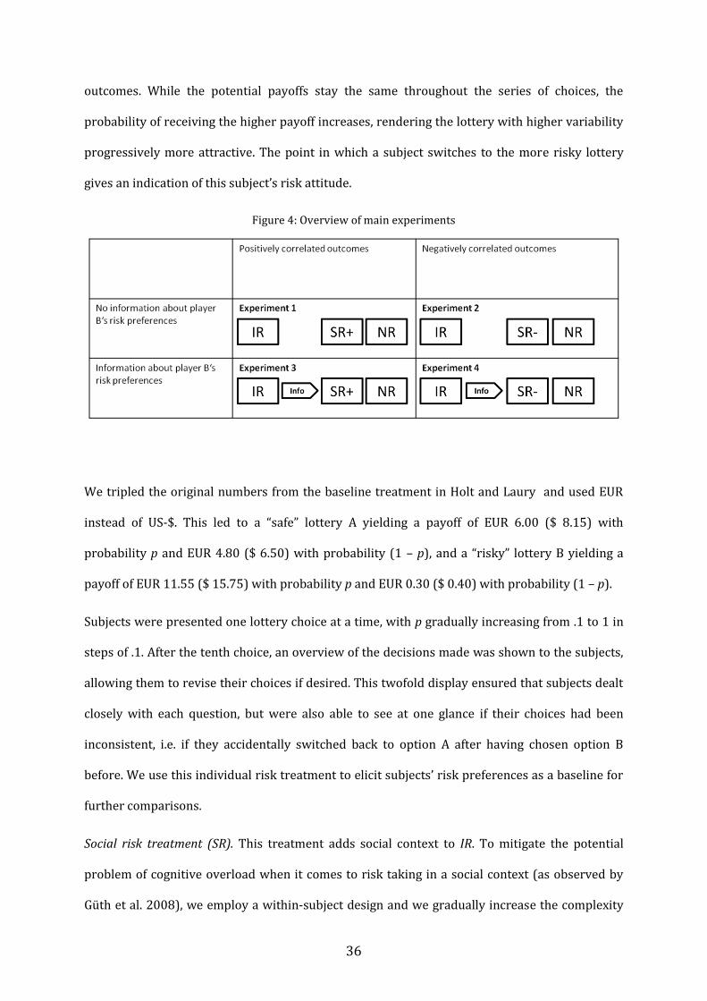
36

outcomes. While the potential payoffs stay the same throughout the series of choices, the

probability of receiving the higher payoff increases, rendering the lottery with higher variability

progressively more attractive. The point in which a subject switches to the more risky lottery

gives an indication of this subject’s risk attitude.

Figure 4: Overview of main experiments

We tripled the original numbers from the baseline treatment in Holt and Laury and used EUR

instead of US-$. This led to a “safe” lottery A yielding a payoff of EUR 6.00 ($ 8.15) with

probability p and EUR 4.80 ($ 6.50) with probability (1 – p), and a “risky” lottery B yielding a

payoff of EUR 11.55 ($ 15.75) with probability p and EUR 0.30 ($ 0.40) with probability (1 – p).

Subjects were presented one lottery choice at a time, with p gradually increasing from .1 to 1 in

steps of .1. After the tenth choice, an overview of the decisions made was shown to the subjects,

allowing them to revise their choices if desired. This twofold display ensured that subjects dealt

closely with each question, but were also able to see at one glance if their choices had been

inconsistent, i.e. if they accidentally switched back to option A after having chosen option B

before. We use this individual risk treatment to elicit subjects’ risk preferences as a baseline for

further comparisons.

Social risk treatment (SR). This treatment adds social context to IR. To mitigate the potential

problem of cognitive overload when it comes to risk taking in a social context (as observed by

Güth et al. 2008), we employ a within-subject design and we gradually increase the complexity

37

of the task by presenting the individual choice problems first (IR) and only then adding social

context always in a second step (SR). The only exception to this is our Experiment 5.

Subjects were randomly and anonymously assigned to participant types A and B, and each

participant A was matched to one participant B. Participant A now had to decide on one lottery

for both her and participant B. Participant B made the same decisions to avoid differences in

working efforts or clues about the participant type, but she was informed that her decisions

were only hypothetical and would not be paid out. Role assignment and group composition

remained the same for the whole course of the experiment, which was communicated to the

subjects.

Correlation of payoffs (SR+, SR-). The social risk treatment was played in two variations. In SR+,

payoffs were perfectly positively correlated, so each participant B received exactly the same

payoff as the corresponding participant A. In SR-, payoffs in the risky lottery B were perfectly

negatively correlated; when participant A received the high payoff, participant B received the

low payoff and vice versa. Bolton and Ockenfels (2010) – and similarly Bohnet et al. (2008) –

found that ex-post inequality resulting from negatively correlated payoffs does not influence the

willingness to take risks. By including both variations, our present study checks the validity and

the robustness of these findings in a very different context. Most importantly, Bolton and

Ockenfels (2010) had each participant making only one binary choice, where one option was

always a safe choice, and the risky option included identical prospects to oneself and the

counterpart with each outcome being realized with 50% probability. In the present study, on the

other hand, following Holt and Laury (2002), participants had to make a series of choices, where

all alternatives are risky, involve a large range of probabilities, and in the social context

prospects are not always identical.

Information (Info). Furthermore, we varied the amount of information subjects received about

the risk preferences of their counterpart. In those experiments including the info stage,

participants A were presented the overview screen from the IR treatment filled in by their

counterpart, and were thus fully aware of participant B’s risk taking profile. In the experiments

38

without information, participants A had to take the social lottery choices without knowing

whether the affected participant B was more or less risk averse than herself.

No risk treatment (NR). The no risk treatment measured social preferences in a risk-free

environment. In the first two experiments, this was done by implementing a classic dictator

game, giving participant A the opportunity to divide a total sum of 12 EUR between herself and

participant B. In the remaining experiments, to increase consistency and comparability of the

applied measures, we replaced the dictator game by binary choices that correspond to the

expected values of the lotteries in SR-.

3.2.2 Procedure

Sessions were run during the period from April 2011 to January 2012 in the Cologne Laboratory

for Economic Research, University of Cologne, Germany. Experiments were programmed in

zTree (Fischbacher 2007). Subjects were recruited from the Cologne student body using the

online recruitment system ORSEE (Greiner 2004). Each of the seven experiments was played by

64 subjects (so that we have 32 dictator decisions in each social context decision task), leading

to a total of 448 participants. The four main experiments described below took 45 - 55 minutes

each, and students earned EUR 8.55 on average including a show-up fee of EUR 2.50 with a

standard deviation of 3.10 (the minimum was EUR 2.80, and the maximum EUR 14.05). All

payments were made anonymously.

In order to avoid income effects, we implemented the strategy method and informed

participants beforehand that one out of all their decisions would be randomly drawn to be

relevant for their earnings. After all subjects had made their choices, one participant drew a card

to determine the payoff-relevant decision. If necessary, a second threw a die to determine the

outcome of the respective lotteries. Appendix B contains the instructions.

3.2.3 Results

Our experimental design provides three main measures to describe subjects’ risk and social

preferences. The number of safe choices in the individual risk treatment without social context

39

indicates individual risk aversion; the number of safe choices with social context indicates social

risk aversion. In both cases, a higher number of safe choices corresponds to higher risk aversion.

Inequality aversion is quantified by measuring either the amount of money transferred to

participant B (experiments 1 - 2) or the number of choices that lead to equal payoffs

(experiment 3 - 7) in the respective no risk treatment.

In our analyses we disregard the hypothetical choices of subjects of participant type B and use

only the data from subjects of type A for our analysis. Out of the 128 subjects who were assigned

the role of participant A, four subjects (3.13 %) exhibited inconsistent preferences by choosing

option A after having chosen option B before. We did not exclude these subjects; excluding them

would not change our main results. If not stated otherwise, we take as the null hypothesis that

risk taking is not affected by social context. In the following, we summarize our main results.

Result 1: Risk taking is not affected by inequality aversion.

We start with the observation that the kind of fairness (or inequality aversion) observed in risk-

free environments does not correlate with the patterns of risk taking that we observe in our

experiments. First, changing risk taking in the presence of social context might indicate a general

concern for the well-being of others. Therefore, one might expect a correlation between the

pattern of fairness in NR and changes in risk taking behavior when we move from IR to SR (we

refer to the difference between individual and social risk aversion as within-difference).

However, there is no evidence for this. With the exception of Experiment 4, the Spearman

correlation coefficients are small (.156, .148, .081, .403, in Experiments 1, 2, 3 and 4,

respectively) and insignificant (p values are .156, .148, .081, .403, respectively).

Second, in Experiments 2 and 4, payoffs of participant A and B are perfectly negatively

correlated and necessarily lead to ex-post inequality. In contrast, both subjects will always get

the same payoff in Experiments 1 and 3, where we induced positively correlated payoffs.

Assuming that ex-post inequality causes disutility, the risky option should be less attractive with

negatively correlated payoffs. Using an Independent Samples Wilcoxon rank-sum test, we cannot

reject the null hypothesis that the distribution of within-difference is the same with negatively

40

and positively correlated payoffs, regardless of whether the data is pooled across Info and

NoInfo or not. In fact, the mean within-difference in the experiments with information is exactly

the same (.34). In the experiments without information, the within-difference is higher with

negatively (.50) than with positively correlated payoffs (.22), but the difference in distributions

is insignificant (p = .140). This indicates that the corresponding observation in Bolton and

Ockenfels (2010) is robust, suggesting that procedural fairness concerns are not restricted to

simple, symmetric fifty-fifty lotteries. We also searched for other evidence for simple fairness

concerns, such as whether there is more risk taking when expected outcomes are more equal,

but could not find any.23 Because we confirm that there are no differences, we pool the SR- and

SR+ data in the following. That said, the next results demonstrate that social context significantly

and robustly affects social behavior, yet in ways not captured by simple fairness models.

Result 2: Risk aversion increases if the risk is extended to another subject.

It has been observed that social context can lead to less risk taking. For instance, groups act

more risk averse than individuals (Baker et al. 2008, Masclet et al. 2009), and subjects make less

risky choices when acting as an agent for a second party rather than deciding for themselves

(Charness and Jackson 2009, Reynolds et al. 2009), and if the risk is extended to another person.

Therefore, we expect subjects to be more risk averse in social than in individual decisions. In

fact, in all experimental conditions, adding social context leads to an increase in risk aversion.

We use a Related Samples Wilcoxon signed-rank test to test for differences in individual and

social risk aversion. Without information, the average number of safe choices increases

significantly from 5.56 to 5.92 (p = .006); with information, the average number of safe choices

increases from 5.94 to 6.28 (p = .008).

Result 3: If risk is extended to another subject whose risk preferences are unknown,

subjects adjust their risk preferences toward the mean.

23 This is not to say that fairness does not play a role at all. For instance, Bolton and Ockenfels (2010) demonstrate that simple fairness concerns affect the willingness to take risks if the alternative option is either a fair or an unfair safe outcome. But we do not find such evidence in the Holt-Laury environment.

41

In Experiments 1 and 2, individual risk aversion and within-difference are significantly

negatively correlated (Spearman’s Rho = -.406, p = .001). In total, 18 subjects increase the

number of safe choices with social context while five subjects decrease it. This proportion gives a

first indication of a higher willingness to adjust risk taking if this results in increasing rather

than decreasing risk aversion, although the magnitude of the adjustment is almost symmetric

here. The mean increase is 1.67, the mean decrease is 1.4, which is not significantly different

(Wilcoxon signed-rank test, p = .675). All subjects who decrease the number of safe choices have

above-average risk preferences, and 13 out of 18 subjects who increase their safe choices have

below-average risk preferences.24 The mean overall risk taking without social context is 5.56;

while the subjects increasing their safe choices with social context exhibit an individual risk

aversion of 4.61 on average, the mean individual risk aversion for those subjects decreasing

their safe choices is 6.40. The difference is highly significant (Wilcoxon rank-sum test, p = .009).

Result 4: If risk is extended to another subject whose risk preferences are known,

subjects adjust their risk preferences toward the second participant’s risk preferences.

Subjects adjust their risk preferences more often and to a higher degree if the second

participant exhibits a higher risk aversion.

In Experiment 3 and 4, subjects were informed about their counterparts' individual risk

aversion and thus able to adjust their risk preferences toward their partners' if desired. We refer

to the difference in individual risk aversion of participant A and participant B as between-

difference. 33 out of 64 subjects changed their risk profile in the social setting. 28 out of these 33

subjects adjusted their preferences towards their respective partner’s risk profile. The

correlation between within- and between-difference is positive and highly significant with

Spearman’s Rho being .628 (p < .001). However, subjects react more often and stronger if their

partner is more risk averse, leading to both a regression effect and increased risk aversion with

social context. If participant B is less risk averse than participant A, participant A decreases the

number of safe choices by .28 on average; if participant B is more risk averse than participant A,

24 Accordingly, the standard deviation decreases from 1.582 to 1.504, but the difference is not significant (Variance ratio test, p = .34).

42

the mean increase in participant A’s number of safe choices is 1.11. The difference in absolute

magnitude is highly significant (Wilcoxon rank-sum test, p < .001).

3.3 Additional tests

We ran three additional experiments to check the robustness of our setting and investigate

alternative interpretations of our results.

3.3.1 Experimental design

The regression to the mean effect (Result 3) might be due to subjects’ desire to conform with

average behavior. However, the effect might also stem from a correction of an error in the first

series of decision and thus be mostly independent of the social context introduced in the second

series of decisions. If a participant makes a mistake in the first treatment and corrects it in the

second, this correction is more likely to move her switching point closer to the average rather

than away from it (for a similar argument, see Cooper and Rege 2011, p. 100). To be able to

distinguish between these explanations, we conducted Experiment 5, which differs from

experiment 1 only by the fact that the first and second treatment are reversed.

Figure 5: Overview experiments 5, 6 and 7

Experiment 6 is designed to test whether the adjustment in stage 2 of the experiment, after

learning about the decisions of participant B, is due to the added social context (Result 4) or to

the information per se. As in Experiments 3 and 4, subjects play the individual risk treatment, are

matched to another participant, and are then informed about the other participant’s preferences.

Unlike experiments 3 and 4, however, they are then facing an individual risk treatment again.

43

In Experiment 7, subjects are first confronted with the individual risk treatment. In a second

step, this treatment is repeated, but before each choice subjects are informed about their own

decision in the first part and the decisions of five other players from previous experiments. The

third part consists of the social risk treatment, where subjects of player type A decide for

themselves and a passive player. As in the second part, they are informed about their own

decision and the decision of five other players in the individual risk treatment prior to each

choice, not including the corresponding information of their participant B.25 As in all previous

experiments, the no risk treatment is employed as the last part. We refer to the information that

was given to the participants as low and high signal. The low signal consisted of information

from five participants who were risk prone and chose 3, 4, 4, 5 and 5 times the safe decision,

respectively. The high signal consisted of information from risk averse participants who chose 7,

7, 8, 8 and 9 times the safe decision, respectively. This way we can directly measure the effect of

social information (see Cooper and Rege 2011 for a similar approach).

3.3.2 Procedure

The procedure was analogous to the main experiments. Sessions were run in January 2012 in

the Cologne Laboratory for Economic Research, University of Cologne, Germany. Each of the

three experiments was played by 64 subjects. Sessions took 45 - 55 minutes and students earned

EUR 9.04 on average including a show-up fee of EUR 2.50, with a standard deviation of 2.438

(the minimum was EUR 6.18, the maximum EUR 14.05). All payments were made anonymously.

3.3.3 Results

Result 5: If individual and social risk treatment are played in reversed order, there is no

adjustment effect as in our Result 3.

If the regression to the mean effect is due to correction of errors, we should find the same

convergence in Experiment 5, where treatment 1 and 2 are played in reversed order. Moreover,

since the social risk treatment is more cognitively challenging than the individual risk treatment

and therefore more likely to cause errors (if at all), the correction effect should be even more

25 Subjects know that they are not informed about the preferences of participant B.

44

pronounced than in Experiment 1. However, we do not find a convergence of switching points

from treatment 1 (social risk) to treatment 2 (individual risk), as shown in Table 2.

Table 2: Individual and social risk aversion depending on order

Individual risk aversion Social risk aversion Experiment 1 and 2 (IR – SR – NR) N = 64

5.56 (1.58)

5.92 (1.51)

Experiment 5 (SR – IR – NR) N = 32

5.81 (1.45)

5.84 (1.37)

Standard deviations in parentheses

Thus, we do not find support for the hypothesis that the effect found in our main experiments

was due to correction of errors. That we do not find an effect in the opposite direction either can

be explained by the fact that the first treatment induced a social context, which may carry over

to the subsequent treatment and exert an influence on judgments, comparisons and decisions

(see, e.g., Posten et al. 2012 and the references therein for related evidence in psychology). This

view is corroborated by the fact that, unlike in Experiment 1 and 2, there is no significant

difference between mean individual and social risk aversion (Wilcoxon signed-rank test, p =

.815), and the within-difference in Experiments 1 and 2 is weakly significantly higher than in

Experiment 5 (Wilcoxon rank-sum test, p = .066).

Result 6: Social information on other participants’ choices per se triggers an adjustment

effect. The adjustment effect is further increased when risk taking affects a passive

player.

Table 3: Individual and social risk aversion with information

Individual risk aversion Social risk aversion/ individual risk aversion

with information Experiment 3 and 4 (IR – info – SR - NR) N = 64

5.94 (1.49)

6.28 (1.29)

Experiment 6 (IR – info – IR - NR) N = 64

6.02 (1.69)

6.05 (1.33)

Standard deviation in parentheses

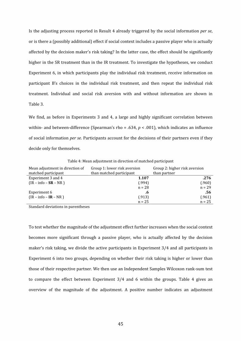
45

Is the adjusting process reported in Result 4 already triggered by the social information per se,

or is there a (possibly additional) effect if social context includes a passive player who is actually

affected by the decision maker's risk taking? In the latter case, the effect should be significantly

higher in the SR treatment than in the IR treatment. To investigate the hypotheses, we conduct

Experiment 6, in which participants play the individual risk treatment, receive information on

participant B’s choices in the individual risk treatment, and then repeat the individual risk

treatment. Individual and social risk aversion with and without information are shown in

Table 3.

We find, as before in Experiments 3 and 4, a large and highly significant correlation between

within- and between-difference (Spearman’s rho = .634, p < .001), which indicates an influence

of social information per se. Participants account for the decisions of their partners even if they

decide only for themselves.

Table 4: Mean adjustment in direction of matched participant

Mean adjustment in direction of matched participant

Group 1: lower risk aversion than matched participant

Group 2: higher risk aversion than partner

Experiment 3 and 4 (IR – info – SR – NR )

1.107 (.994) n = 28

.276 (.960) n = 29

Experiment 6 (IR – info – IR – NR )

.6 (.913) n = 25

.56 (.961) n = 25

Standard deviations in parentheses

To test whether the magnitude of the adjustment effect further increases when the social context

becomes more significant through a passive player, who is actually affected by the decision

maker's risk taking, we divide the active participants in Experiment 3/4 and all participants in

Experiment 6 into two groups, depending on whether their risk taking is higher or lower than

those of their respective partner. We then use an Independent Samples Wilcoxon rank-sum test

to compare the effect between Experiment 3/4 and 6 within the groups. Table 4 gives an

overview of the magnitude of the adjustment. A positive number indicates an adjustment

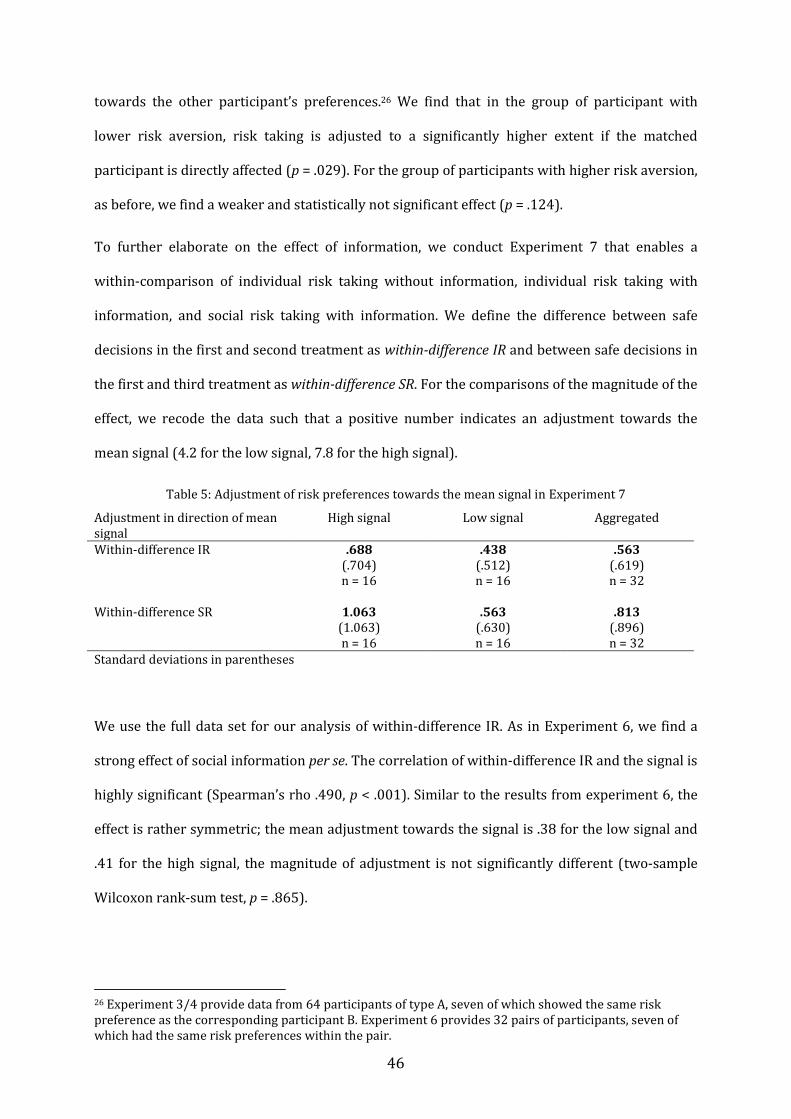
46

towards the other participant’s preferences.26 We find that in the group of participant with

lower risk aversion, risk taking is adjusted to a significantly higher extent if the matched

participant is directly affected (p = .029). For the group of participants with higher risk aversion,

as before, we find a weaker and statistically not significant effect (p = .124).

To further elaborate on the effect of information, we conduct Experiment 7 that enables a

within-comparison of individual risk taking without information, individual risk taking with

information, and social risk taking with information. We define the difference between safe

decisions in the first and second treatment as within-difference IR and between safe decisions in

the first and third treatment as within-difference SR. For the comparisons of the magnitude of the

effect, we recode the data such that a positive number indicates an adjustment towards the

mean signal (4.2 for the low signal, 7.8 for the high signal).

Table 5: Adjustment of risk preferences towards the mean signal in Experiment 7

Adjustment in direction of mean signal

High signal Low signal Aggregated

Within-difference IR .688 (.704) n = 16

.438 (.512) n = 16

.563 (.619) n = 32

Within-difference SR 1.063

(1.063) n = 16

.563 (.630) n = 16

.813 (.896) n = 32

Standard deviations in parentheses

We use the full data set for our analysis of within-difference IR. As in Experiment 6, we find a

strong effect of social information per se. The correlation of within-difference IR and the signal is

highly significant (Spearman’s rho .490, p < .001). Similar to the results from experiment 6, the

effect is rather symmetric; the mean adjustment towards the signal is .38 for the low signal and

.41 for the high signal, the magnitude of adjustment is not significantly different (two-sample

Wilcoxon rank-sum test, p = .865).

26 Experiment 3/4 provide data from 64 participants of type A, seven of which showed the same risk preference as the corresponding participant B. Experiment 6 provides 32 pairs of participants, seven of which had the same risk preferences within the pair.

47

For the comparison between within-difference IR and within-difference SR, the data of the

passive participants are dropped. Table 5 shows the mean within-differences for low and high

signals. The adjustment effect in the aggregated data set is significantly higher in the social risk

treatment than in the individual risk treatment (Wilcoxon signed-rank test, p = .033), but the

differences within the groups are not or only weakly significant (p = .097 for high signal, p = .157

for low signal). Furthermore, we see a tendency for stronger adjustment with risk averse signals

compared to risk prone signals, but the difference is insignificant (p = .330 for within-difference

IR, p = .152 for within-difference SR).

We finally note that we do not find a correlation between the willingness to adjust individual

risk taking and social risk taking in the no risk treatment in any of the control experiments,

further supporting Result 1.

3.4 Conclusion

Extending previous observations by Bolton and Ockenfels (2010) and Rohde and Rohde (2011)

to a standard Holt and Laury (2002) setting, we find little evidence that risk taking is affected by

ex post inequality, yet robustly confirm evidence that risk taking becomes more conservative if

the risk is extended to another person. More importantly, by our within subject design, our

study can add two new observations on the nature of social risk taking. First, social context

makes risk taking being more conform with others' risk attitudes. Specifically, decision makers

generally adjust their risk taking towards what they know others do in a similar context.

Because of the increased conservatism in social context, the effect is more pronounced if the

adjustment results in less risk-taking. Second, the more the risky choices are embedded in a

social context, the more pronounced are these effects. While assigning a subject to a group and

informing her about the other participants’ choices is sufficient to trigger an adjustment, the

effect is significantly stronger if a subject’s risk taking has a direct influence on a second

participant. We conclude that conformism and conservatism systematically affect risk taking in a

social context.

48

3.5 Appendix

Sample instructions (Experiment 3)

49

(…)

50

51

52

(…)

53

54

(…)

55

56

4 A hero game27

4.1 Introduction

Many social and economic settings require coordinated behavior in order to establish a

favorable outcome. We investigate a situation in which exactly one person should make a costly

effort to increase the total outcome and ideally reach the socially efficient solution. This “heroic”

willingness to volunteer for the good of the group coins the type of “hero game” we discuss. The

coordination property hinges on the fact that only one person within a group should step in as

the hero to establish a social optimum.

The type of dilemma discussed in this paper occurs in various economic situations. One example

is open source software development: If a certain software application is needed, simultaneous

programming wastes resources since only the superior solution will be used subsequently.

Upfront coordination on a single developer would be of benefit to avoid efficiency losses. Similar

cases can be found if players represent companies. Taking an example from an Industrial

Organization context, the hero game describes the problem that occurs if several companies

develop an industry standard and the best standard will be adopted by all companies.

We examine two different versions of the hero game, varying the costs subjects have to bear to

increase social efficiency. In line with standard theory, we find that these costs have a strong

influence on subjects’ willingness to exert effort. However, in the second version of the game, a

coordination game with multiple equilibria, we observe several deviations from standard

theory. We discuss social preferences, risk aversion, and ex-post rationality as potential

approaches to organize our data.

The remainder of this chapter is organized as follows. In section 4.2, we present the hero game

and discuss related literature. In section 4.3, we describe our experimental design, theoretical

predictions, and experimental procedure. We present the experimental results in section 4.5.

Section 4.6 concludes.

27 This study is joint work with Christoph Feldhaus (Feldhaus and Stauf 2012).

57

4.2 The hero game

In a hero game, n players form a group and simultaneously choose a positive effort level e from a

given interval. Each player’s individual payoff depends on her own effort and on the maximum

effort chosen within her group. The payoff function that defines the hero game is

where is the effort chosen by an individual i, and is the highest effort chosen by any other

member of her group. Parameters a and b determine the feasible payoff based on the highest

chosen effort and individual effort costs. Payoff function and strategy space are common

knowledge. In this study, we are only concerned with the symmetric version of the game, so

factors a and b and the available strategies e are identical for all players.

A player’s payoff decreases in her own effort and increases in the maximum of her group. Thus,

each player prefers someone to exert a high effort over everyone choosing the minimum effort

level; however, everyone prefers someone else to do so. As long as a > b/n, efficiency increases

in the highest invested effort. Optimally, everyone chooses the minimum effort except for one

player; this single hero provides a public good by increasing the payoffs of all group members

including herself at costs be. A further group member providing the good at a lower or equal

effort level increases the total costs, but not the benefits. Hence, her additional investment is in

vain.

The game discussed here is equivalent to the best shot public good game broadly defined by

Hirshleifer (1983). Hirshleifer discusses summation, weakest link, and best shot as three

different functions to transform individual contributions into public goods, which he refers to as

social composition functions. The case most often discussed with respect to public good games is

the summation composition function, the public good simply being based on the sum of all

58

contributions. With weakest link and best shot, the public good is determined only by the lowest

and the highest individual contribution, respectively.28

While Hirshleifer only defines general social composition functions without any restrictions

regarding the protocol or the number of players, a subsequent experimental test only considers

2-person games (Harrison and Hirshleifer 1989) that are played simultaneously and

sequentially. Starting with Prasnikar and Roth (1992) who compare the sequential 2-person

variant to the ultimatum game, the term best shot game is commonly used for a sequential 2-

person game where payoffs are determined by individual contribution and maximum

contribution (e.g. Bolton and Ockenfels 2000, Carpenter 2002, Duffy and Feltovich 1999).

Therefore, we use the term hero game to differentiate it from the predominant definition of the

best shot game.

The general structure of the hero game always leads to a situation where every player wants

someone else to be the hero who exerts an effort higher than emin. Furthermore, as long as a >

b/n, finding exactly one hero is socially optimal. Varying the ratio between a and b, however,

changes whether being the hero can be individually rational, and whether a hero is found in

equilibrium. The parameter ratio leads to three structurally different versions of the hero game

which we will discuss in more detail in the following.

4.2.1 Version 1 (a b)

If the costs b of playing a higher effort exceed the additional profit a, the hero has to pay to

increase the payoffs of her group members to the extent that her payoff is lower than the

outcome of choosing emin. However, for b/n < a < b, the social benefit of choosing e > emin is higher

than the individual costs, so being a hero increases the total payoff of the group. However, being

a hero is not individually rational. Because emin is a strictly dominant strategy, each player

28 It is important to note that Hirshleifer disregards the usual restriction that the marginal per capita return (MPCR) from the group account in public good games is lower than 1 (and higher than ). If this condition holds, it is individually rational not to invest in the public good, while it is socially optimal if everyone invests their entire endowment, which creates a social dilemma. The MPCR is defined as the ratio of benefits to costs for moving a single token from the individual to the group account. See Ledyard (1995) for an overview.

59

chooses emin in the unique Nash equilibrium. Thus, the theoretical prediction is that no hero is to

be found.

This version of the hero game relates to social dilemma games, a prominent example being the

public good game. In a linear public good game, a person that contributes never profits

individually, since the MPCR of the public good is lower than the individual investment. Although

the social optimum is realized if all participants invest their whole endowments, equilibrium

theory suggests that no one invests.

In this version of the hero game as well as in social dilemma games, the Nash-equilibrium is not

the social optimum. However, there is a crucial difference between the games. Social dilemmas

are usually defined as games where the social optimum is Pareto-better than the Nash

equilibrium (Dawes 1980). This is not the case in the hero game: the aggregated payoff is higher

in the social optimum, but the hero receives a lower payoff than in equilibrium.29

4.2.2 Version 2 (a b)

Case 1: a = b.

Being a rather special case, this version will not receive further attention in this study, but we

briefly discuss the strategic implications of this case for the sake of completeness. The hero’s

individual benefit from the provision of a higher effort level equals her costs. Given that

everyone else chooses emin, any choice of strategy yields zero profits; hence, the hero is

indifferent between all available effort levels. However, if any other player chooses e > emin, emin is

the best reply, as a higher effort increases the costs without changing the benefits. It follows that

any combination of n − 1 players choosing emin and the remaining player choosing any effort level

is a Nash equilibrium.

Case 2: a b.

If the profit a of becoming the hero is larger than the costs b of doing so, each player prefers to

choose a high number if everyone else chooses the minimum, but everyone prefers someone else

29 A solution that is Pareto-better than the equilibrium could only be achieved intertemporally in a repeated setting and would require several players to take turns in being the hero.

60

to do so, which causes a coordination problem. The hero game is rendered a coordination game,

which is defined as a game containing multiple equilibria which requires coordinated behavior

of the players.30 This version of the hero game contains n Nash equilibria in pure strategies in

which one player chooses emax while the remaining players choose emin. Players therefore have to

coordinate their behavior in order to find exactly one hero who chooses emax. Payoffs in

equilibrium are asymmetric across players; all group members benefit from the high effort

exerted by the hero, but only the hero bears the costs for reaching the social optimum.

Nevertheless, it is individually rational for the hero to choose a high effort if (and only if)

everyone else freerides.

In an equilibrium in mixed strategies, players randomize only between efforts that are best

replies in pure strategies (see e.g. Gibbons 1992). Here, players will choose either emin or emax.

The sure payoff from choosing emax is aemax – bemax. Choosing emin yields a payoff of aemax – bemin if

at least one other player chooses emax, and a payoff of aemin – bemin if all group members choose

emin. In a symmetric mixed strategy equilibrium, each participant chooses emax with the same

probability p. It follows that the probability of everyone else choosing emin is (1 – p)n-1, and the

probability of finding at least one hero among the n − 1 other players is

1 – (1 – p)n-1. In equilibrium, the expected payoff of choosing emin equals the sure payoff of

choosing emax:

The left hand side of the equation shows the sure payoff of choosing emax, while the right hand

side shows the expected payoff from choosing emin if everyone else chooses emax with probability

p. Solving the equation for p yields

which is the individual probability of becoming a hero and choosing the maximum effort emax in a

symmetric mixed strategy equilibrium. The probability p* increases in a and decreases in b; it

30 For surveys on coordination games see e.g. Kagel and Roth (1995), Camerer (2003).

61

becomes more likely that a person chooses emax if the relative costs of doing so are low. The

expected payoff of a mixed strategy equilibrium equals the sure payoff aemax – bemax from

choosing the maximum emax.

Structurally similar to the hero game in this version are order statistic games and the volunteer’s

dilemma. The most widely known instance of order statistic games is the minimum effort game

(Van Huyck et al. 1990). Each member of a group of n players chooses an effort level e from a

closed interval. The game is defined by the payoff function

.

Each player’s best response to any min{e-i} is to choose her own effort equally. Thus, all

combinations of all players choosing the same effort levels are Nash equilibria. Contrary to the

hero game, equilibria in the minimum effort game can be Pareto ranked, as individual and global

profits increase in emin. Analogous to the minimum effort game, the hero game can be seen as the

corresponding maximum effort game. However, order statistic games are usually defined as

games where a deviation from the order statistic induces costs (Devetag and Ortmann 2007).

This is not the case in the hero game: if one player chooses the maximum effort level, everyone

profits individually from a deviation.

Furthermore, for , the hero game closely resembles the volunteer’s dilemma introduced by

Diekmann (1985).31 In the volunteer’s dilemma game, each one of n members of a group faces

the binary decision whether to volunteer or not. Only one person is needed to produce a public

good; if one person volunteers, all payoffs increase while only the volunteer bears the costs.

Additional volunteering does not further increase payoffs. The worst individual and global

outcome is realized if none of the participants volunteers.

The main difference between the hero game and the volunteer’s dilemma is the higher number

of available strategies in the hero game. Although this does not change the resulting equilibria,

31 Diekmann (1986, p. 187 – 188) uses a broader definition of dilemmas: “Social dilemmas (…) are defined in this article more generally as situations where the pursuit of self-interest might lead to the collectively bad and paradox result of a Pareto-inferior payoff vector.”

62

the opportunity to choose from multiple effort levels might change empirical results by

increasing perceived strategic uncertainty.32 Furthermore, the volunteer’s dilemma is by

definition restricted to cases where the volunteer herself profits from choosing to volunteer. As

a consequence, only this case has been tested experimentally so far. By allowing any ratio

between the parameters a and b, the hero game offers a wider scope of application and covers

situations where the hero needs to pay in order to increase efficiency.

4.3 Experiment

4.3.1 Design

In this initial study, we test version 1 (a < b) and version 2 (a > b). Regarding version 1, we study

the willingness of subjects to bear individual costs to reach a social optimum. With respect to the

coordination game in version 2, we aim to investigate to what extent groups are able to realize a

socially desirable outcome without an explicit coordination device, and whether they are able to

enhance efficiency and coordination success over time.

Each group consists of four players. The parameters a and b and the available efforts e are based

on the order statistic games proposed by Van Huyck et al. (1990, 1991). In each period,

participants choose integer effort levels e 1,...,7 which determine the payoffs. Additionally,

participants are asked to provide an unincentivized estimation of the highest number in their

group including their own. After each period, participants are informed about the highest

number chosen within their group and their payoffs. The payoffs are displayed in the ficticious

experimental currency unit ECU with an exchange rate of 1 ECU = .08 Euro. The instructions are

written in a neutral manner without reference to the name of the game.33

The potential payoffs of the treatments are shown in Table 6 and Table 7. These tables are

presented to the participants in the instructions of their respective treatment. The numbers on

32 As we will see in Chapter 4.5, intermediary strategies are indeed played to a substantial extent although they should not be chosen in equilibrium. 33 The instructions can be found in Appendix B, pp. 75 - 76.

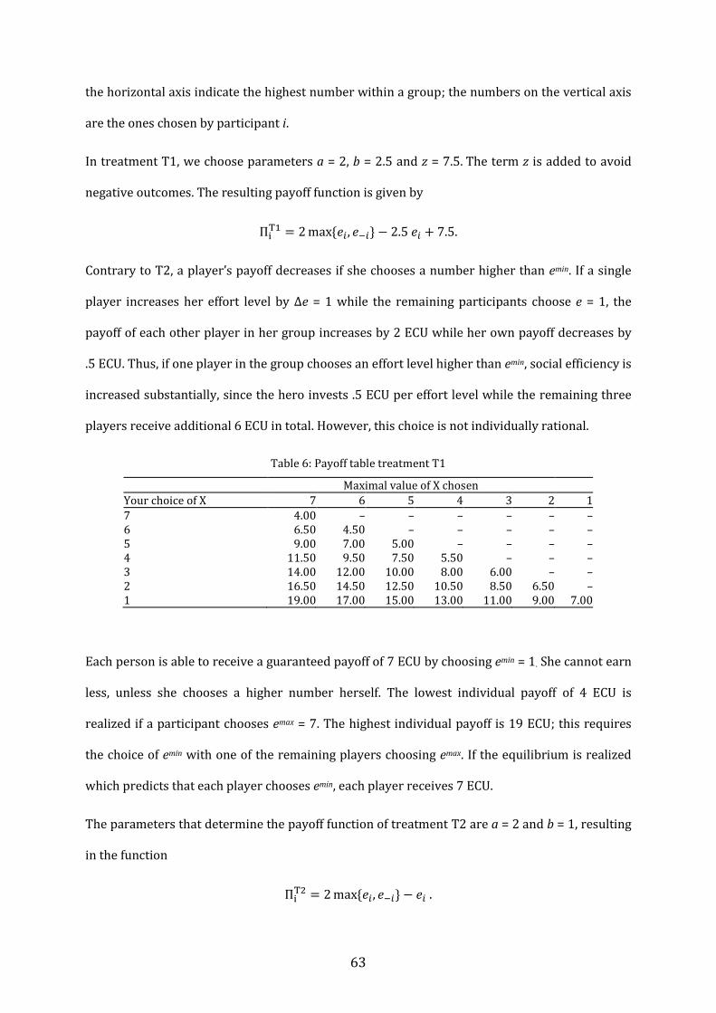
63

the horizontal axis indicate the highest number within a group; the numbers on the vertical axis

are the ones chosen by participant i.

In treatment T1, we choose parameters a = 2, b = 2.5 and z = 7.5. The term z is added to avoid

negative outcomes. The resulting payoff function is given by

Contrary to T2, a player’s payoff decreases if she chooses a number higher than emin. If a single

player increases her effort level by Δe = 1 while the remaining participants choose e = 1, the

payoff of each other player in her group increases by 2 ECU while her own payoff decreases by

.5 ECU. Thus, if one player in the group chooses an effort level higher than emin, social efficiency is

increased substantially, since the hero invests .5 ECU per effort level while the remaining three

players receive additional 6 ECU in total. However, this choice is not individually rational.

Table 6: Payoff table treatment T1

Maximal value of X chosen

Your choice of X 7 6 5 4 3 2 1

7 4.00 – – – – – – 6 6.50 4.50 – – – – – 5 9.00 7.00 5.00 – – – – 4 11.50 9.50 7.50 5.50 – – – 3 14.00 12.00 10.00 8.00 6.00 – – 2 16.50 14.50 12.50 10.50 8.50 6.50 – 1 19.00 17.00 15.00 13.00 11.00 9.00 7.00

Each person is able to receive a guaranteed payoff of 7 ECU by choosing emin = 1. She cannot earn

less, unless she chooses a higher number herself. The lowest individual payoff of 4 ECU is

realized if a participant chooses emax = 7. The highest individual payoff is 19 ECU; this requires

the choice of emin with one of the remaining players choosing emax. If the equilibrium is realized

which predicts that each player chooses emin, each player receives 7 ECU.

The parameters that determine the payoff function of treatment T2 are a = 2 and b = 1, resulting

in the function

64

The lowest individual payoff in this version is 1 ECU which is realized if each player chooses emin.

The highest feasible payoff equals 13 ECU and results from a choice of emin while at least one

other player in the group plays emax.

Table 7: Payoff table treatment T2

Maximal value of X chosen

Your choice of X 7 6 5 4 3 2 1

7 7.00 – – – – – – 6 8.00 6.00 – – – – – 5 9.00 7.00 5.00 – – – – 4 10.00 8.00 6.00 4.00 – – – 3 11.00 9.00 7.00 5.00 3.00 – – 2 12.00 10.00 8.00 6.00 4.00 2.00 – 1 13.00 11.00 9.00 7.00 5.00 3.00 1.00

If all other players choose emin, an increase in own effort of Δe = 1 results in an increase in own

payoff by 1 ECU, while the others’ payoffs increase by 2 ECU. Hence, the hero always receives

less than the other players, but she still earns more from volunteering herself in comparison to a

case where no one does. Again, the highest sure payoff that can be achieved in this treatment is

7 ECU per period which is realized if a player chooses emax. In this case, her payoff does not

depend on the decisions of other participants. The highest overall payoff is 46 ECU, if exactly

one hero is found who chooses the highest effort while everyone else chooses emin; the lowest

overall payoff is 4 ECU if everyone chooses emin.

4.3.2 Procedure

We conducted four experimental sessions with 32 participants each in September 2010 in the

Cologne Laboratory for Economic Research (CLER), University of Cologne, Germany. Two

sessions were conducted per treatment. Participants were recruited randomly by email with the

experiment recruiting software ORSEE (Greiner 2004). About 60 % of the participants were

students of the Faculty of Management, Economics and Social Sciences. 48 % were female, and

the mean subject was 24.3 years old.

The experiment was programmed in zTree (Fischbacher 2007). The actual experiment was

preceded by a short test to ensure that the participants understood the rules of the

65

experiment.34 In both treatments, the 32 subjects who took part in a session were randomly

assigned to four groups of eight players. The experiment was played for ten rounds. In each

round, each group was split into two subgroups of four players. This procedure leads to 16

independent observations per treatment in the first round and eight in the following (eight

groups of eight). Subjects were told that the groups were randomly rematched in each round,

but they were not informed about these details of the rematching procedure.

After each round, participants were informed about the highest number in the group and their

payoffs. This procedure was repeated ten times. After the tenth round, the payoffs were summed

up, and subjects were informed about their total payoff in ECU and the resulting payoff in Euro

including a show-up fee of 2.50 Euro. Afterwards, participants were asked to fill out a

questionnaire asking for demographic data. Finally, payoffs were paid out privately in cash.

Participants earned 8.79 Euro on average (9.38 in T1, 8.19 Euro in T2). Each session took

between 40 and 50 minutes.

4.4 Hypotheses

In this section, we derive hypotheses for our experiment. We interpret the repeated game with

strangers matching as a series of one-shot games. Accordingly, we only consider equilibria of the

one-shot game.

In treatment T1, the unique equilibrium is that every player chooses emin, which means that no

hero is to be found.35

Hypothesis 1. All players in T1 choose strategy emin.

Treatment T2 has several equilibria. Game theory predicts n pure strategy equilibria where one

player chooses emax while the remaining players choose emin. Moreover, there is a symmetric

34 In order to pass the test, each participant had to choose four integers between one and seven which represented the choices of a group of four players. Participants then had to determine the payoffs for each of the ficticious players using the payoff table. If they entered a wrong payoff, the input was rejected and they had to try again. This procedure was repeated once. In the second run, participants were not allowed to choose the same numbers as in the first one to enhance learning effects. 35 According to standard theory, this is also the only equilibrium of the finitely repeated game even if we employed a partners matching.

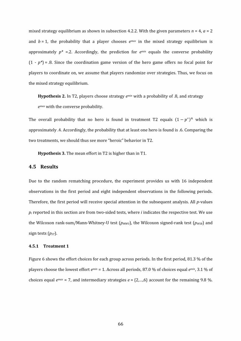
66

mixed strategy equilibrium as shown in subsection 4.2.2. With the given parameters n = 4, a = 2

and b = 1, the probability that a player chooses emax in the mixed strategy equilibrium is

approximately p* =.2. Accordingly, the prediction for emin equals the converse probability

(1 - p*) = .8. Since the coordination game version of the hero game offers no focal point for

players to coordinate on, we assume that players randomize over strategies. Thus, we focus on

the mixed strategy equilibrium.

Hypothesis 2. In T2, players choose strategy emin with a probability of .8, and strategy

emax with the converse probability.

The overall probability that no hero is found in treatment T2 equals which is

approximately .4. Accordingly, the probability that at least one hero is found is .6. Comparing the

two treatments, we should thus see more “heroic” behavior in T2.

Hypothesis 3. The mean effort in T2 is higher than in T1.

4.5 Results

Due to the random rematching procedure, the experiment provides us with 16 independent

observations in the first period and eight independent observations in the following periods.

Therefore, the first period will receive special attention in the subsequent analysis. All p-values

pi reported in this section are from two-sided tests, where i indicates the respective test. We use

the Wilcoxon rank-sum/Mann-Whitney-U test (pMWU), the Wilcoxon signed-rank test (pWSR) and

sign tests (pST).

4.5.1 Treatment 1

Figure 6 shows the effort choices for each group across periods. In the first period, 81.3 % of the

players choose the lowest effort emin = 1. Across all periods, 87.0 % of choices equal emin, 3.1 % of

choices equal emax = 7, and intermediary strategies e = {2,…,6} account for the remaining 9.8 %.

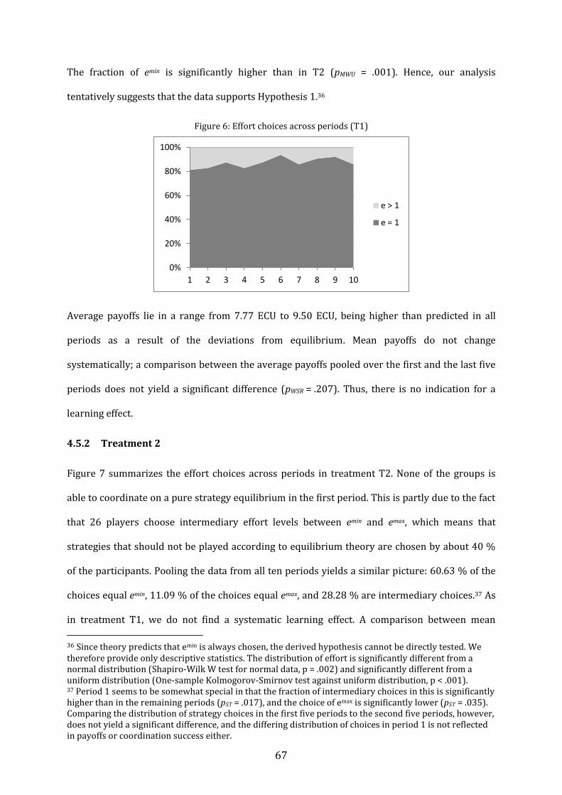
67

The fraction of emin is significantly higher than in T2 (pMWU = .001). Hence, our analysis

tentatively suggests that the data supports Hypothesis 1.36

Figure 6: Effort choices across periods (T1)

Average payoffs lie in a range from 7.77 ECU to 9.50 ECU, being higher than predicted in all

periods as a result of the deviations from equilibrium. Mean payoffs do not change

systematically; a comparison between the average payoffs pooled over the first and the last five

periods does not yield a significant difference (pWSR = .207). Thus, there is no indication for a

learning effect.

4.5.2 Treatment 2

Figure 7 summarizes the effort choices across periods in treatment T2. None of the groups is

able to coordinate on a pure strategy equilibrium in the first period. This is partly due to the fact

that 26 players choose intermediary effort levels between emin and emax, which means that

strategies that should not be played according to equilibrium theory are chosen by about 40 %

of the participants. Pooling the data from all ten periods yields a similar picture: 60.63 % of the

choices equal emin, 11.09 % of the choices equal emax, and 28.28 % are intermediary choices.37 As

in treatment T1, we do not find a systematic learning effect. A comparison between mean

36 Since theory predicts that emin is always chosen, the derived hypothesis cannot be directly tested. We therefore provide only descriptive statistics. The distribution of effort is significantly different from a normal distribution (Shapiro-Wilk W test for normal data, p = .002) and significantly different from a uniform distribution (One-sample Kolmogorov-Smirnov test against uniform distribution, p < .001). 37 Period 1 seems to be somewhat special in that the fraction of intermediary choices in this is significantly higher than in the remaining periods (pST = .017), and the choice of emax is significantly lower (pST = .035). Comparing the distribution of strategy choices in the first five periods to the second five periods, however, does not yield a significant difference, and the differing distribution of choices in period 1 is not reflected in payoffs or coordination success either.

0%

20%

40%

60%

80%

100%

1 2 3 4 5 6 7 8 9 10

e > 1

e = 1

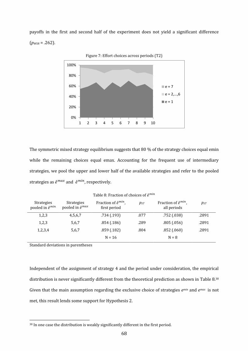
68

payoffs in the first and second half of the experiment does not yield a significant difference

(pWSR = .262).

Figure 7: Effort choices across periods (T2)

The symmetric mixed strategy equilibrium suggests that 80 % of the strategy choices equal emin

while the remaining choices equal emax. Accounting for the frequent use of intermediary

strategies, we pool the upper and lower half of the available strategies and refer to the pooled

strategies as and , respectively.

Table 8: Fraction of choices of

Strategies pooled in

Strategies pooled in

Fraction of

first period pST

Fraction of

all periods pST

1,2,3 4,5,6,7 .734 (.193) .077 .752 (.038) .2891

1,2,3 5,6,7 .854 (.186) .289 .805 (.056) .2891

1,2,3,4 5,6,7 .859 (.182) .804 .852 (.060) .2891

N = 16 N = 8

Standard deviations in parentheses

Independent of the assignment of strategy 4 and the period under consideration, the empirical

distribution is never significantly different from the theoretical prediction as shown in Table 8.38

Given that the main assumption regarding the exclusive choice of strategies emin and emax is not

met, this result lends some support for Hypothesis 2.

38 In one case the distribution is weakly significantly different in the first period.

0%

20%

40%

60%

80%

100%

1 2 3 4 5 6 7 8 9 10

e = 7

e = 2,…,6

e = 1

69

4.5.3 Treatment comparison

Comparing the results of the first period between treatments, we find that the mean effort is

significantly higher in T2 than in T1 (pMWU <.001). While the minimum is played by 55 % in T2, it

is played by more than 80 % in T1. The treatment differences in the initial period are also found

if we pool the data over all periods. In T1, mean maxima and mean efforts per independent

observation across all periods are significantly lower than in T2 (pMWU <.001). This fully supports

Hypothesis 3. Moreover, we find that the fraction of intermediary strategy choices is

significantly higher in T2 than in T1 (pMWU = .002). We will discuss potential reasons for the high

fraction of intermediary strategy choices in T2 in the next section.

4.6 Discussion

Although players are rematched after each period, the repetition of the game means that

individual behavior may depend on the respective player’s history, leading to a systematic

behavioral pattern. In treatment T2, this pattern may or may not enhance coordination success.

To account for this potential influence, we suggest learning direction theory (Selten and Stoecker

1986) as an approach to organize our data.

Learning direction theory predicts that changes in players’ behavior in a repeated game with

feedback follow a principle of ex-post rationality. Ex-post rationality means that if participants

change their behavior, they adjust it such that they do in the current period what would have

been better in the previous one (Selten 1998) rather than in the opposite direction.39 Table 9

shows the predicted and the actual adjustments after a given condition. Note that players are

only informed about their own effort choice and the maximum effort choice max{e} in the group.

Accordingly, the experience condition is determined by these two pieces of information.40

39 Ex-post rationality does not imply that players always change their behavior. Learning direction theory, in turn, does not predict that behavioral changes always follow ex-post rationality, but only that this happens more often than randomly expected. For a detailed explanation see Selten (1998). 40 Moreover this means that, if a player chooses the maximum effort herself, she does not know whether somebody else has chosen the same effort. Whether an individual that set an effort ei > 4 and determined the maximum experiences an impulse to adjust her effort, thus depends on the respective player’s beliefs about the effort choices of the remaining players. Therefore, it is not possible to predict a clear impulse in

70

If the maximum effort in the group of player i is lower than 4, the player would have earned

more if she had chosen ei = emax independent of whether she has determined the maximum,

which leads to an upward impulse. If the maximum effort is greater than 4 and player i has

chosen ei > 1, but has not determined the maximum, the payoff of player i would have been

greater if she had chosen ei = emin, leading to a downward impulse. Finally, if the maximum effort

is greater than 4 and player i has chosen ei = emin, there should be no impulse at all.

Table 9: Conditions, predicted impulses and adjustments

ei max{e} Predicted impulse

Downward adjustment

No adjustment Upward adjustment

ei = max{e}, ei = 1

max{e} = 1 upwards adjustment

-- 50 (65.79 %)

26 (34.21 %)

pFE = .022

ei = max{e}, ei > 1

max{e} < 4 upwards adjustment

10 (9.26 %)

56 (51.85 %)

42 (38.89 %)

pFE < .001

max{e} = 4 ambiguous 15 (51.72 %)

6 (20.69 %)

8 (27.57 %)

-

max{e} > 4 ambiguous 62 (72.09 %)

18 (20.93 %)

6 (6.98 %)

-

ei < max{e}, ei = 1

max{e} < 4 upwards adjustment

-- 43 (61.42 %)

27 (38.57 %)

pFE = .004

max{e} = 4 ambiguous -- 48 (81.36 %)

11 (18.64 %)

-

max{e} > 4 no adjustment -- 133 (89.26 %)

16 (10.76 %)

pFE < .001

ei < max{e}, ei > 1

max{e} < 4 upwards adjustment

2 (33.33 %)

0 (0.00 %)

4 (66.67 %)

pFE = .025

max{e} = 4 ambiguous 6 (50.00 %)

1 (8.33 %)

5 (41.67 %)

-

max{e} > 4 downwards adjustment

35 (61.40 %)

14 (24.56 %)

8 (14.04 %)

pFE < .001

Total 130 (22.57 %)

319 (55.38 %)

127 (22.05 %)

Observations in line with predictions are in bold print.

Since in the majority of the cases subjects do not change their effort levels, we compare the

distribution of adjustments after an impulse with the overall distribution. The results of Fisher’s

exact test are reported in the last column of Table 9. Accounting for the fact that there is a

general tendency to not adjust the individual effort level, our tests suggest that people react to

impulses in the direction predicted by ex-post rationality.

this condition. The same holds for any condition in which the maximum max{e} equals 4, because in this case, strategy emin and emax result in the same payoff of 7 ECU.

71

These results, however, are potentially biased in favor of the ex-post rationality approach. If

players’ behavior follows some random pattern, a low effort is generally more likely to be

followed by an upward shift than a high effort. In order to control for this effect, we test the

hypothesis that the changes in efforts are caused by impulses against the null hypothesis that

the changes follow a random pattern.41 We find that the effort choices are significantly more

often in line with ex-post rationality than a random combination of the same effort choices

would be (pWST = .017), thus supporting the prediction of learning direction theory.

Our results indicate that subjects adjust their behavior to what would have been better in the

previous period in spite of the random rematching process. On average, participants thus react

to the same impulses in the same way. Since strategies are substitutes, however, this behavioral

pattern does not improve coordination. Beyond organizing the data, ex-post rationality might

therefore serve as an explanation for why players are not able to enhance efficiency over the

course of time.

Ex-post rationality, however, should lead to a decrease of the fraction of intermediary strategies,

but there is no indication for such a process.42 In the following, we will briefly discuss two

possible explanations for the frequent occurrence of intermediary strategy choices. First,

subjects might exhibit other-regarding preferences. Second, subjects might not consider the

strategic nature of the game and behave similarly to a setting with exogenous uncertainty.

Considering other-regarding preferences, efficiency concerns would not change the set of best

replies in treatment T2 because the pure strategy equilibrium equals the socially efficient

41 Adapting the approach of Ockenfels and Selten (2005), we calculate two scores for each subject. The real score indicates the proportion of effort choices that are consistent with ex-post rationality, disregarding the observations following conditions in which we cannot predict an unambiguous impulse. The fictitious score is calculated analogously over all permutations of this subject’s effort choices - holding the effort choices of the remaining players constant - and divided by the number of permutations. Ex-post rationality would result in the real score being higher than the fictitious score, whereas random effort choices would lead to equal scores. We find that the mean real score is .619, while the mean fictitious score is .535. Table 10 in Appendix A additionally depicts the fraction of choices that are consistent/ inconsistent with ex-post rationality. 42 See section 4.5.2.

72

outcome.43 A similar reasoning holds for altruism. If a player increases her effort, the payoff of

the remaining players is affected only if she can determine the maximum. In this case, choosing

emax increases both individual payoff and overall welfare; otherwise, choosing emin maximizes

individual payoff while leaving overall welfare unaffected.

If a subject holds the belief that every other player chooses a low number, combined with a

strong sense of fairness with regard to disadvantageous inequality, anticipated envy could keep

the subject from choosing the highest possible effort. While this explanation is in line with the

ERC framework (Bolton and Ockenfels 2000), the model by Fehr and Schmidt (1999) would not

predict such a behavior. Given that a subject holds the belief that one other player will choose

emax, choosing an intermediary effort reduces inequality, but the subject’s outcome would

decrease without any direct influence on the hero’s outcome. Again, burning money for the sake

of reducing advantageous inequality is in principle possible in the ERC framework, but excluded

in the model by Fehr and Schmidt (1999).44

The second explanation is based on evidence showing that subjects treat strategic uncertainty

similar to exogenous risks (Heinemann et al. 2009). Supposing that players disregard the

implications of strategic games, and that they exhibit risk aversion, the choice of intermediary

strategies can in principle be rationalized assuming appropriate beliefs. We illustrate this with a

numerical example. For a realistic representation of risk preferences, we use the estimation of

average risk preferences by Holt and Laury (2002), which is based on the power-expo utility

function (Saha 1993)45

43 Preferences for efficiency might serve as an explanation for the deviations from equilibrium in treatment T1. Since standard theory organizes the data fairly well, however, we omit treatment T1 in this discussion. 44 In both cases, however, this behavior would presume an excessively high parameter for equality preferences in the ERC framework. 45 The form of the power-expo function includes constant absolute risk aversion ( and constant relative risk aversion as special cases; for intermediary levels of and as estimated by Holt and Laury, the function implies increasing relative risk aversion and decreasing absolute risk aversion. For a detailed discussion see Holt and Laury (2002).

73

We substitute and for the respective parameters and estimated by Holt

and Laury (2002) to calculate utilities for the strategies ei = 1,…,7.

Figure 8 depicts the expected utility for a given strategy if a player believes that emax will be

played by at least one other player with a probability of .6, while emin will be played by all

remaining players otherwise.46 In this case, every intermediate strategy yields a higher expected

utility than strategies emin and emax. Thus, assuming that players disregard the strategic nature of

the game, risk aversion might serve as an explanation for the frequent choice of strategies that

are never a best reply.

Figure 8: Expected utility of strategies ei = 1,..., 7

Both explanations presuppose a particular set of beliefs. Based on the data generated in this

experiment, we are not able to test these explanations or distinguish between them. However,

we believe that this aspect deserves further attention, as it may help to shed light on the general

questions whether other-regarding preferences play a role in strategic games, and how strategic

uncertainty is perceived and processed.

46 Note that this would require that players hold systematically wrong beliefs; the empirical probability that at least one player chooses emax is .369, and the empirical probability that all players choose emin is .119.

3.8

3.85

3.9

3.95

4

4.05

4.1

1 2 3 4 5 6 7

EU(ei)

Strategy ei

74

4.7 Conclusion

In treatment T1, where the costs subjects have to bear to increase social efficiency exceed

individual gains, we find that subjects choose the lowest available effort in the vast majority of

cases, which matches the standard theoretical predictions fairly well. In treatment T2, where

subjects are individually better off if they exert effort if no one else does, we find that a large

fraction of subjects chooses intermediary effort levels which are never best replies, which is

inconsistent with standard theory. We discuss social preferences and risk aversion as potential

explanations for these choices, but our data is insufficient to distinguish between these

explanations. If we account for the frequent use of intermediary strategies, the empirical results

come close to the mixed strategy equilibrium. There is no indication that groups are able to

enhance efficiency in the course of time. We propose ex-post rationality as an explanation for the

lack of coordination success. If the majority of players react to the same signals in the same way,

the adjustment process does not enhance coordination. The differences between the treatments

are as predicted; mean efforts are higher if the costs of exerting effort are lower.

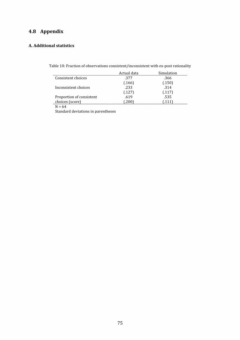
75

4.8 Appendix

A. Additional statistics

Table 10: Fraction of observations consistent/inconsistent with ex-post rationality

Actual data Simulation Consistent choices .377

(.166) .366

(.150) Inconsistent choices .233

(.127) .314

(.117) Proportion of consistent choices (score)

.619 (.200)

.535 (.111)

N = 64 Standard deviations in parentheses

76

B. Instructions (English translation)

Welcome and thank you for participating in this experiment. Please do not communicate with

other participants from now on until the end of the experiment. Noncompliance with this rule

will lead to your exclusion from the experiment.

Please read these instructions thoroughly. Please raise your hand should you have any questions

while reading the instructions or during the experiment. One of the experimenters will then

come to you and answer your question. Before the experiment starts, we will run a short test in

order to check whether you understood the instructions. All participants have received the same

instructions.

Payment and anonymity

You can earn money during this experiment. How much money you earn depends on your own

decisions as well as on the decisions of the other participants. During the experiment your

payoffs are calculated in a virtual currency, the so called experimental currency units (ECU). 1

ECU is equal to .08 Euro. At the end of the experiment your payoffs will be converted into Euro

and paid out to you in cash. Additionally, you receive a show-up fee of 2.50 Euro for your

appearance.

Your payoff as well as your decisions in the experiment are kept confidential. Participants will

not know with whom they interacted during the experiment, neither during nor after the

experiment.

In this experiment, you will have to take decisions in ten consecutive rounds. In each round you

will form a group with three other participants. This group is matched randomly at the

beginning of each round.

In each round, each participant chooses a number. Possible numbers are 1, 2, 3, 4, 5, 6, and 7.

The highest number of all participants within a group, including your own number, dictates the

potential payoffs.

77

Your payoff in each round (based on your own decision as well as the decisions of the other

members of your group) is shown in the following table:

Your payoff

Highest number within your group Your number 7 6 5 4 3 2 1 7 7.00 – – – – – – 6 8.00 6.00 – – – – – 5 9.00 7.00 5.00 – – – – 4 10.00 8.00 6.00 4.00 – – – 3 11.00 9.00 7.00 5.00 3.00 – – 2 12.00 10.00 8.00 6.00 4.00 2.00 – 1 13.00 11.00 9.00 7.00 5.00 3.00 1.00

The left column represents the number you have chosen, while the upper row indicates the

highest number within your group (including your own number).

Apart from choosing your own number within each round, we ask you to estimate the highest

number of your whole group (including your own number).

After each round you will be able to see your own number, the highest number of your group

and your payoff from the respective round. Afterwards the next round begins.

At the end of all ten rounds, your payoffs are summed up, converted into Euro and displayed on

your screen together with the 2.50 Euro show-up fee. Finally, you will receive a questionnaire,

which we ask you to complete while the payments are prepared.

78

5 Speak up, hero! The impact of pre-play communication on

volunteering

5.1 Introduction

Consider a situation in which a manager delegates a task to a team by sending out an email to all

team members, relying on the team’s ability to coordinate. The task needs to be done urgently,

and only one single person is needed to perform it. If several team members work on the task

simultaneously, only the best outcome will be of use for the manager, while the effort of the

other team members will be in vain. Each team member wants the task to be done in order to

avoid consequences for the employment relationship. Therefore, if nobody else is willing to

perform the task, every team member prefers to do the job herself. However, the team member

has to exert effort to perform the job which is costly in terms of disutility of labor, so everyone

prefers someone else to do it.

The situation described above can be modeled as a hero game (Feldhaus and Stauf 2011). The

worst individual and global outcome is realized if there is no “hero”, which means that, in the

above example, all team members refuse to perform the task. If at least one person decides to

choose the hero strategy and works on the task, all payoffs including her own payoff are

increased, but the hero is worse off relative to the other players as her action requires a costly

effort. An additional hero does not further increase payoffs, so she decreases global efficiency as

her investment is in vain. Similar situations can be found in various economic contexts and can

include both individuals and companies as players.47 Any situation where exactly one player

chooses to exert effort is an equilibrium in this game, leading to a coordination problem.48 A

natural means to solve this is communication.

We conduct a series of experiments to study if pre-play communication is a useful means of

improving coordination success in the context of the hero game. For this purpose, we introduce

47 Taking an example from the field of Industrial Organization, the process of simultaneously developing an industry standard, the best of which will be adopted by all companies, can be modeled in a similar way. 48 For an overview of coordination failure in experiments see Devetag and Ortmann (2007).

79

a cheap talk stage prior to the simultaneous effort choices. Cheap talk is defined as having no

direct payoff implications and being costless and nonbinding (e.g. Farrell 1987). In our

teamwork setting, the latter criterion implies that team members are not able to punish retreats

from verbal commitment; even if one team member signals that she will undertake the task, she

can retreat from her commitment, and the manager will hold the entire team responsible for the

unfinished job.

There is some experimental evidence on the efficiency-improving characteristics of cheap talk

from coordination games in general. Cooper et al. (1992) investigate a 2-person stag hunt game

and find less coordination failure with one-way communication and almost no coordination

failure with simultaneous two-way communication.49 Burton and Sefton (2004) find an increase

in equilibrium play due to communication in a two-player 3x3 game with a unique equilibrium

and a dominated safe strategy. Blume and Ortmann (2007) study order statistic games and find

that the possibility to send messages facilitates participants’ coordination on the Pareto-

dominant equilibrium, even for more than two players, and for both median and minimum

games.

Although these examples demonstrate the positive effect of cheap talk on coordination, they

stem from games with symmetric equilibria, which generate equal payoffs for all participants ex

post. A distinctive feature of the problem discussed here, however, is the asymmetry that is

necessarily present if players coordinate on a pure strategy equilibrium. For the battle of the

sexes, a two person game with asymmetric equilibria, it has been shown that one-way

communication significantly improves coordination; while two-way communication helped to

overcome coordination problems to some extent, it performed worse than one-way

communication (Cooper et al. 1989). To the best of our knowledge, however, no studies exist on

the effect of communication on coordination and efficiency in an asymmetric coordination game

with more than two players. Furthermore, the battle of the sexes game implies that players are

49 One-way communication is defined as letting one randomly chosen player send a message containing information about the strategy she is going to play, while two-way communication means that both players send messages simultaneously.

80

always interested in successful coordination on pure strategy equilibria, since even coordination

on the respective worse pure strategy equilibrium is strictly preferred over playing mixed

strategies. This is not the case in the hero game, where the expected payoff from the mixed

strategy equilibrium equals the payoff of being a hero, which means that the incentive to engage

in pre-play negotiations is substantially weaker.

The remainder of this chapter is organized as follows. In section 5.2, we discuss related

theoretical and experimental literature. We derive our hypotheses in section 5.3. We describe

the experimental design and procedure in sections 5.4 and 5.5, and we present our results in

section 5.6. We discuss efficiency concerns as an additional approach to better organize our data

in sections 5.7 and 5.8. Section 5.9 concludes.

5.2 Theory

5.2.1 The hero game

In the game discussed here, n players decide whether to exert a costly effort ei. Effort choices are

made simultaneously. The payoff of player i is given by

with a > b > 0, and ei, ej ϵ {e1, …, em}. In the following, we denote the lowest and the highest

available effort e1 and em by emin and emax, respectively.

Each player in the group profits if one player exerts a high effort, but the costs are borne by that

player only. The maximin strategy is given by the hero strategy emax, guaranteeing a safe payoff

of independent of the strategy choices of the remaining players.

This game has multiple equilibria. In the following, we restrict the analysis to the choice of

strategies emin and emax, since these are the only strategies that can be best replies. Therefore, any

strategy combination that includes a strategy different from emin and emax cannot be an

equilibrium. In spite of offering more strategies, the equilibria in the hero game thus equal the

equilibria in the related volunteer’s dilemma (Diekmann 1985).

81

A hero game (or volunteer’s dilemma) with n players has n pure strategy Nash equilibria, each

consisting of one of the players choosing effort level emax while the remaining players choose emin.

In the symmetric mixed strategy equilibrium, all players are indifferent between the strategies

emax and emin; since strategy emax leads to a safe payoff , the expected payoff

must be the same. Thus, in the hero game, there exists a symmetric mixed strategy equilibrium

where all players choose strategy emax with probability

and strategy emin is played with the converse probability. 50

The higher the costs b of playing strategy emax compared to the benefits a, and the higher the

number of players n, the lower the probability that a given player chooses emax in the symmetric

mixed strategy equilibrium. The resulting overall probability to find no hero among the players

equals

Note that the overall probability that no player within a group chooses emax is increasing in the

number of players n, suggesting that larger groups are less likely to educe a hero. This result by

Diekmann (1985) is in line with a well-known phenomenon in psychology referred to as

diffusion of responsibility, describing the diminishing willingness to help in emergencies in large

crowds (Darley and Latané 1968). Vice versa, this means that reducing the number of players

that mix over strategies increases the probability that at least one hero is found. This case will be

of special interest for our analysis of one-way communication below.

Beyond the analysis of Diekmann (1985), we consider asymmetric mixed-strategy equilibria.

50 See Diekmann (1985).

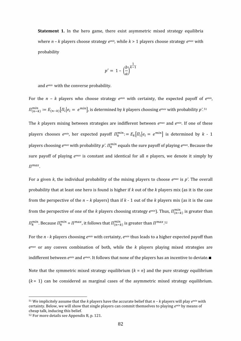
82

Statement 1. In the hero game, there exist asymmetric mixed strategy equilibria

where n – k players choose strategy emin, while k > 1 players choose strategy emax with

probability

and emin with the converse probability.

For the n – k players who choose strategy emin with certainty, the expected payoff of emin,

, is determined by k players choosing emax with probability p’. 51

The k players mixing between strategies are indifferent between emax and emin. If one of these

players chooses emin, her expected payoff is determined by k - 1

players choosing emax with probability p’. equals the sure payoff of playing emax. Because the

sure payoff of playing emax is constant and identical for all n players, we denote it simply by

For a given k, the individual probability of the mixing players to choose emax is p’. The overall

probability that at least one hero is found is higher if k out of the k players mix (as it is the case

from the perspective of the n – k players) than if k - 1 out of the k players mix (as it is the case

from the perspective of one of the k players choosing strategy emin). Thus, is greater than

. Because

= , it follows that is greater than .52

For the n - k players choosing emin with certainty, emin thus leads to a higher expected payoff than

emax or any convex combination of both, while the k players playing mixed strategies are

indifferent between emin and emax. It follows that none of the players has an incentive to deviate.∎

Note that the symmetric mixed strategy equilibrium (k = n) and the pure strategy equilibrium

(k = 1) can be considered as marginal cases of the asymmetric mixed strategy equilibrium.

51 We implicitely assume that the k players have the accurate belief that n – k players will play emin with certainty. Below, we will show that single players can commit themselves to playing emin by means of cheap talk, inducing this belief. 52 For more details see Appendix B, p. 121.

83

Analogous to diffusion of responsibility, the probability that at least one hero is found decreases

in the number of mixing players k. In the case of k = 1, the individual probability to choose emax as

well as the overall probability to find at least one hero equals 1. Accordingly, efficiency increases

if k decreases and is highest for k = 1, i.e. in the pure strategy equilibrium.

5.2.2 Communication

To investigate whether communication can serve as a means to mitigate the coordination

problem, we study a two-stage game where the hero game is preceded by a communication

stage. In the communication stage, players simultaneously announce to their groups which effort

they intend to choose in the subsequent stage. In the following, we will refer to the first stage as

signaling stage and to the second as effort choice stage. The message space is limited to signals

corresponding to the available strategies, and a message that announces strategy ek is denoted as

sk. Furthermore, we assume that message sk is understood by all players as “the sender of this

message intends to play effort ek”. However, announcements are non-binding; senders are free

to choose an effort different from the one they have announced.

We will investigate two communication structures and compare them with a baseline treatment

where the hero game is played without any preceding communication. First, in the one-way

communication treatment, one player is randomly chosen and sends a message to all group

players. Second, in the multi-way communication treatment, all players simultaneously send

messages to the remaining players in their group.

Non-binding and costless communication prior to a game is referred to as cheap talk (Farrell

1987). However, it has been empirically and theoretically shown that if players’ interests are

sufficiently similar, cheap talk can be informative (Crawford 1998). This is especially the case for

coordination problems with symmetric equilibrium outcomes, where players’ payoffs depend

only on matching others’ strategies. In the hero game, players are faced with a coordination

problem, but pure strategy equilibria always involve asymmetric payoffs. Therefore, the

credibility of messages in the cheap talk stage deserves closer attention.

84

To assess the value of signals53 with one-way communication, we adopt two widely used criteria.

First, we analyze whether a signal is self-committing (Farrell 1987). A self-committing signal, if

believed by the receivers, creates incentives for the sender to take the announced action. This is

equivalent as to say that the strategy indicated by the signal and the respective responses of the

remaining players form a Nash equilibrium in the succeeding subgame. Second, we follow

Aumann (1990) in imposing the additional requirement that a message is credible if the sender

wants it to be believed if and only if she indeed plans to take the corresponding action. This

property is referred to as self-signaling (Farrell and Rabin 1996). If these requirements are not

met, we follow Farrell (1987) in assuming that the respective set of messages leads to the

babbling equilibrium where all messages are considered meaningless and therefore ignored,

resulting in a mixed strategy equilibrium.

In the game discussed here, a sender who intends to play emax is indifferent between all available

signals, since she will get the same outcome independently of the effort choices of others. Thus,

the question of how to treat indifference is of crucial relevance, but, to the best of our

knowledge, has not been explicitly addressed in the literature. A strict interpretation of the

definition by Farrell and Rabin would render all signals in the hero game noncredible. However,

we consider it more plausible to assume that a player will send an untruthful signal only if she

has an incentive to do so.54

With simultaneous multi-way communication, the optimal reaction does not only depend on the

individual message sent, but also on the messages of all other players, which hampers the

analysis of the credibility of individual signals. In line with the approaches by Farrell (1987) and

Cooper et al. (1989), we thus focus on self-commitment.55 We assume that, whenever the

strategies corresponding to a set of cheap talk messages constitute an equilibrium in the

subsequent game, these strategies will be played.

53 The terms “message” and “signal” are used synonymously. 54 While Aumann (1990) and Farrell and Rabin (1996) provide only verbal definitions of the credibility conditions, Baliga and Morris (2002) offer a formalization. They omit the case of indifference in their formal discussion, but, in the analysis of an exemplary game, implicitly make the same assumption as is made here. 55 Experimental work by Charness (2000) suggests that self-commitment is the more crucial requirement for credibility in coordination games, while self-signaling plays only a minor role.

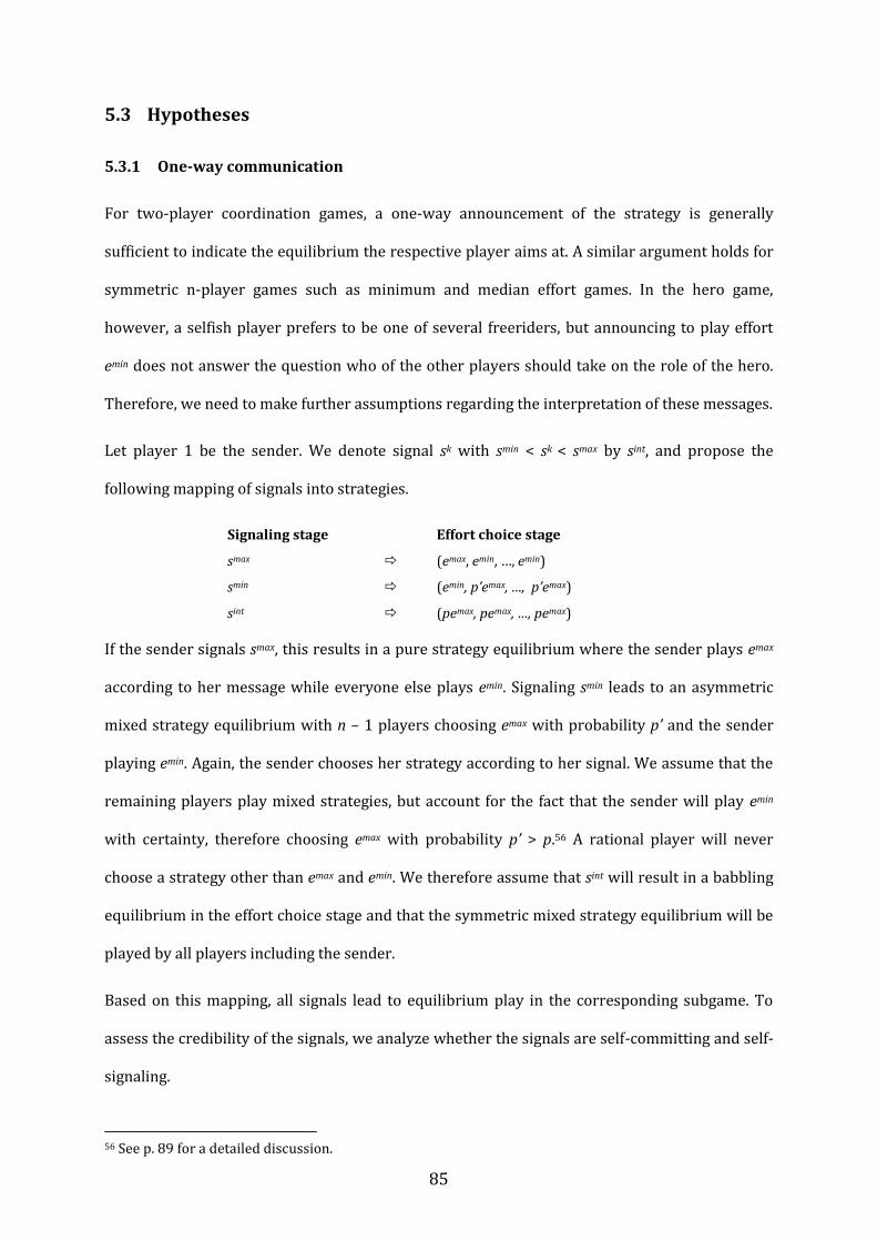
85

5.3 Hypotheses

5.3.1 One-way communication

For two-player coordination games, a one-way announcement of the strategy is generally

sufficient to indicate the equilibrium the respective player aims at. A similar argument holds for

symmetric n-player games such as minimum and median effort games. In the hero game,

however, a selfish player prefers to be one of several freeriders, but announcing to play effort

emin does not answer the question who of the other players should take on the role of the hero.

Therefore, we need to make further assumptions regarding the interpretation of these messages.

Let player 1 be the sender. We denote signal sk with smin < sk < smax by sint, and propose the

following mapping of signals into strategies.

Signaling stage Effort choice stage

smax (emax, emin, …, emin)

smin (emin, p’emax, …, p’emax)

sint (pemax, pemax, …, pemax)

If the sender signals smax, this results in a pure strategy equilibrium where the sender plays emax

according to her message while everyone else plays emin. Signaling smin leads to an asymmetric

mixed strategy equilibrium with n – 1 players choosing emax with probability p’ and the sender

playing emin. Again, the sender chooses her strategy according to her signal. We assume that the

remaining players play mixed strategies, but account for the fact that the sender will play emin

with certainty, therefore choosing emax with probability p’ > p.56 A rational player will never

choose a strategy other than emax and emin. We therefore assume that sint will result in a babbling

equilibrium in the effort choice stage and that the symmetric mixed strategy equilibrium will be

played by all players including the sender.

Based on this mapping, all signals lead to equilibrium play in the corresponding subgame. To

assess the credibility of the signals, we analyze whether the signals are self-committing and self-

signaling.

56 See p. 89 for a detailed discussion.

86

Statement 2.1. Signals smin and smax are self-committing.

A signal is self-committing if the announced effort choice and the other players’ best replies form

a Nash equilibrium in the effort choice game. Since only emax and emin can be best replies, only smin

and smax are self-committing signals. ∎

Statement 2.2. Signals smin and smax are self-signaling.

A signal is self-signaling if the sender has no incentive to send it if she in fact intends to choose a

different effort, and if she has no incentive to send a different signal if she intends to choose the

respective effort.

If the sender intends to play emax, she is indifferent between all available signals and has no

incentive to send a signal other than smax. If the sender sends smax, the remaining players will

react by choosing emin, which is the worst possible action from the perspective of the sender. If

the sender wants to choose emin, signaling a low effort increases the chances that another player

in the group chooses emax. She will thus signal smax only if she intends to play emax. Signal smax is

self-signaling.

Since strategy eint with emin < eint < emax is never a best reply, the sender will not choose it,

independent of the signal she sent. Therefore, sint is not self-signaling and leads to the babbling

equilibrium.

If the player intends to play emin, the highest probability that at least one other player chooses

emax can be achieved by signaling smin. Thus, she will always send smin if she wants to play emin. The

only pure strategy the sender would want to play apart from emin is emax, where she would be

indifferent between all signals. Therefore, if she does not intend to choose emin, she has no

incentive to signal smin. Signal smin is self-signaling. ∎

Statement 3. Sending smin and playing emin is an equilibrium of the two-stage game

with one-way communication.

As we have seen above, the symmetric mixed strategy equilibrium as well as playing emax leads to

the same (expected) payoff, making the sender indifferent between sending smax and sint.

87

However, the asymmetric mixed strategy equilibrium following smin leads to a higher expected

payoff for the sender than the other options. Signal smin, followed by the sender playing emin while

everyone else plays emax with probability p’, is therefore an equilibrium of the two-stage game. ∎

Hypothesis 1.1. All senders send smin and choose emin.

Signaling smin and playing emin not only increases the expected payoff of the sender, but also

reduces the overall probability that no hero is found, thereby increasing the expected overall

payoff and the probability to coordinate on an ex-post equilibrium.57

Since smax results in a perfect coordination while signal sint and no signal (in the baseline

treatment) lead to mixed strategies, efficiency should be higher after smax. Signal smin also leads to

mixed strategies, but because of the higher probability to find a hero due to the adjusted

probability p’, efficiency should be higher than after sint or no signal, but still lower than after

smax.

Hypothesis 1.2. Signal smax leads to higher efficiency than signal smin.

Hypothesis 1.3. Signal smin leads to higher efficiency than signal sint or no signal.

5.3.2 Multi-way communication

Two-way communication means that both players in a two-player game simultaneously send

messages to each other. This is transferred to n-player games by letting all players send

messages simultaneously.58 We use the term “multi-way communication” to stretch the point

that there can be more than two players involved in the game, and that all involved players can

send messages.

Two-way communication has been shown to improve coordination and efficiency in games with

symmetric equilibria, but to perform worse than one-way communication in games with

asymmetric equilibria. While a single sender can establish a focal point by sending an

unambiguous message, several players sending messages simultaneously face the same

57 See p. 89. 58 See e.g. Blume and Ortmann (2007).

88

coordination problem as the one in the subsequent game. For this reason, it is not obvious why

multi-way communication should improve coordination success at all.59 For the battle of sexes

game, a two-player game with asymmetric equilibria, Cooper et al. (1989) though find that two-

way communication can lead to improved coordination and higher efficiency. They assume that

if the actions announced by the players in the cheap talk stage constitute an ex-post equilibrium,

i.e. an equilibrium in the payoff-relevant stage, these messages are highly credible and likely to

be followed. If the players’ signals do not match, players choose a mixed strategy in the payoff-

relevant stage. Based on this mapping of signals into strategies, Cooper et al. show that in a

mixed strategy equilibrium of the two-stage game, the less preferred action is signaled with

positive probability in the signaling stage.60 A signaling stage thus offers a second opportunity to

coordinate on the pure strategy equilibrium by chance.

This notion can be directly transferred to a game with more than two players. Given that players

choose a mixed strategy in the signaling stage, we follow Cooper et al. (1989) in assuming that if

the announced efforts constitute an ex-post equilibrium, these efforts are chosen in the effort

choice stage; otherwise, players mix over efforts.61

Hypothesis 2.1. If the messages in the signaling stage constitute an ex-post

equilibrium, this equilibrium will be played in the effort choice stage.

There is, however, a major difference between the hero game and the battle of the sexes game. In

a battle of the sexes game, each player prefers the respective worse pure strategy equilibrium

over the mixed strategy equilibrium, since the latter yields a lower expected payoff. Players thus

have a strong incentive to cooperate to achieve coordination on a pure strategy equilibrium. In

contrast, in the hero game, the mixed strategy equilibrium in the effort stage yields the same

expected payoff as the hero outcome, which is the individually worse outcome of a pure strategy

equilibrium.

59 Consequently, the theoretical analysis of multi-way communication is more problematic and the predictions are weaker than for one-way communication. 60 For a detailed explanation see Cooper et al (1989), p. 572. 61 Since only emin and emax can constitute an equilibrium in the effort choice stage, any constellation including intermediary signals sint also leads to mixed strategies in the effort choice stage.

89

Statement 4. In a mixed strategy equilibrium based on the above assumptions, signal

smax will not be played with positive probability.

If player i signals smax, this always leads to the same expected payoff regardless of the choices of

the remaining players. The same holds for signal sint, which always leads to mixed strategies. If

she signals smin, however, she can achieve a higher payoff by freeriding if exactly one other player

signals smax. Otherwise, she is indifferent between all available signals. Thus, in a mixed-strategy

equilibrium of the two-stage game, players would not play smax with positive probability.62 ∎

Hypothesis 2.2. Signal smax is never chosen.

5.3.3 Treatment comparison

In the previous subsections, we have derived predictions for subjects’ behavior under the

respective communication regimes. In a second step, we compare the effect of the predicted

behavior on efficiency across treatments. Since we predict that all senders in the one-way

communication treatment signal smin and choose emin, leading to a higher probability that exactly

one player chooses emax, we expect higher efficiency with one-way communication than without

communication. We do not expect any difference between a setting with multi-way

communication and one without communication. Based on our prediction that none of the

players will send smax, we predict that multi-way communication results in a babbling

equilibrium in which all messages are ignored.

Hypothesis 3.1. With one-way communication, efficiency is higher than without

communication.

Hypothesis 3.2. There are no differences between multi-way communication and no

communication with regard to efficiency.

62 Note that, as soon as signal smax is assigned a probability of 0, players are indifferent between all remaining signals.

90

5.4 Experimental design

We conduct three treatments implementing the coordination game described above in the effort

choice stage. In treatment 2 and 3, subjects enter an additional communication stage prior to the

effort choice stage. Table 11 shows an overview of the treatments.

Table 11: Treatment overview

Treatment Treatment groups Communication stage Effort choice stage T1: Baseline T1.1 – T1.8 - All players choose effort

levels simultaneously T2: One-way T2.1 – T2.8 In each group, one randomly determined

player sends a message All players choose effort levels simultaneously

T3: Multi-way

T3.1 – T3.8 All players send messages to their group members simultaneously

All players choose effort levels simultaneously

In the effort choice stage, we use an instance of the hero game with strategies and signals ei, si ϵ

{1,...,7}, parameters a = 2, b = 1, the resulting payoff function Πi = 2*max(ei, ej) – ei, and n = 4

players. This instance of the hero game has four Nash equilibria in pure strategies where one

player chooses an effort level of emax = 7 (the hero strategy) while the remaining players choose

emin = 1. Perfectly coordinated equilibrium play leads to an effort choice of 7 in 25 % and 1 in

75 % of all cases, and an average payoff per period of 11.5. In the mixed strategy equilibrium,

emax is played with probability p = 20.6 %, leading to an expected payoff of 7 and an overall

probability to coordinate on an ex-post equilibrium of p = 41.3 %.

The payoff functions and the resulting payoff tables (see Table 12) are identical in all treatments.

In each round, participants choose integer effort levels e 1,...,7 and provide an unincentivized

estimation of the highest effort chosen in their group. The payoffs are displayed in the fictitious

experimental currency unit ECU. In all three treatments, the hero game is played for ten rounds

in groups of four players. Groups are randomly rematched after each round to preclude players

from coordinating by rotating the role of the hero over the course of the game. After each round,

subjects were informed about the maximum effort chosen in their group and their payoffs.

In treatment T2 (one-way communication), each subject is told that one randomly determined

group member, the sender, will send a message to all other players in the group to indicate her

91

strategy choice in the decision stage. We employ the strategy method, asking all subjects to

choose a message which will be sent only if they are chosen to be the sender. In treatment T3

(multi-way communication), all subjects simultaneously send messages to all other group

members. In both treatments, the message space is limited to integers from 1 to 7, reflecting the

possible effort choices.

Table 12: Payoff table

Your payoff Maximum effort choice of all other players

7 6 5 4 3 2 1

Your effort choice

7 7 7 7 7 7 7 7

6 8 6 6 6 6 6 6

5 9 7 5 5 5 5 5

4 10 8 6 4 4 4 4

3 11 9 7 5 3 3 3

2 12 10 8 6 4 2 2

1 13 11 9 7 5 3 1

5.5 Procedure

The two sessions of the baseline treatment with 64 subjects in total were run in September

2010, the four sessions of the one-way and multi-way communication treatments with 128

subjects in total were run in January 2012 in the Cologne Laboratory for Economic Research

(CLER), University of Cologne, Germany. 63 Experiments were programmed in zTree

(Fischbacher 2007). Subjects were recruited from the Cologne student body using the online

recruitment system ORSEE (Greiner 2004). Within one treatment, all subjects received identical

instructions. Questions were answered privately. The experiment was preceded by a short test

to ensure that participants understood the rules of the game.64

The respective treatment was repeated ten times. The rematching was carried out within groups

of eight that were randomly split into subgroups of four in the beginning of each round. Subjects

63 The data from the baseline treatment have already been used in a prior study (Feldhaus and Stauf 2012). 64 To prevent anchoring effects, subjects were asked to type in four random numbers. These numbers represented effort choices of a fictitious group of players. Using the payoff table in the instructions, subjects had to calculate the payoff for each group member and were only able to participate in the experiment after correctly solving the task twice with different numbers.

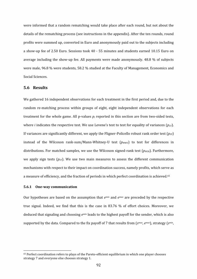
92

were informed that a random rematching would take place after each round, but not about the

details of the rematching process (see instructions in the appendix). After the ten rounds, round

profits were summed up, converted in Euro and anonymously paid out to the subjects including

a show-up fee of 2.50 Euro. Sessions took 40 - 55 minutes and students earned 10.15 Euro on

average including the show-up fee. All payments were made anonymously. 48.8 % of subjects

were male, 96.8 % were students, 58.2 % studied at the Faculty of Management, Economics and

Social Sciences.

5.6 Results

We gathered 16 independent observations for each treatment in the first period and, due to the

random re-matching process within groups of eight, eight independent observations for each

treatment for the whole game. All p-values pi reported in this section are from two-sided tests,

where i indicates the respective test. We use Levene’s test to test for equality of variances (pLV).

If variances are significantly different, we apply the Fligner-Policello robust rank order test (pFP)

instead of the Wilcoxon rank-sum/Mann-Whitney-U test (pMWU) to test for differences in

distributions. For matched samples, we use the Wilcoxon signed-rank test (pWSR). Furthermore,

we apply sign tests (pST). We use two main measures to assess the different communication

mechanisms with respect to their impact on coordination success, namely profits, which serve as

a measure of efficiency, and the fraction of periods in which perfect coordination is achieved.65

5.6.1 One-way communication

Our hypotheses are based on the assumption that emin and emax are preceded by the respective

true signal. Indeed, we find that this is the case in 83.76 % of effort choices. Moreover, we

deduced that signaling and choosing emin leads to the highest payoff for the sender, which is also

supported by the data. Compared to the fix payoff of 7 that results from (smax, emax), strategy (smin,

65 Perfect coordination refers to plays of the Pareto-efficient equilibrium in which one player chooses strategy 7 and everyone else chooses strategy 1.

93

emin) yields a significantly higher mean payoff of 9.128 (pWSR = .022).66 Table 13 gives an

overview of signals and corresponding effort choices.

Table 13: Signals and corresponding effort choices

emin eint emax Total

smin 58 0 3 61

sint 20 13 4 37

smax 16 6 40 62

Total 94 19 47 160

Hypothesis 1.1 states that all players send smin and choose emin. The data does not support this

prediction though. Only 38.28 % of the signals with one-way communication equal smin, which is

significantly lower than 50 % (pWSR = .049) and not significantly different from the number of

smax signals (36.88 %, pWSR = .780).

Moreover, comparing the effort choices of senders and non-senders (see Table 14), we find that

the average effort level chosen by the sender is weakly significantly higher (pWSR = .069), and

that senders choose emax significantly more often (pWSR = .049). Also, compared to players in the

baseline treatment, senders choose a significantly higher effort level (pFP = .003) and choose emax

significantly more often (pMWU = .011).

Table 14: Comparison of effort choices of senders and non-senders

Mean effort Mean frequency of emax Sender (T2) 3.094 (.802) .294 (.135) Non-sender (T2) 2.329 (.387) .150 (.050) Baseline treatment (T1) 2.388 (.209) .111 (.050)

Standard deviations in parentheses

Hypothesis 1.2 states that signal smax leads to higher efficiency than smin; Hypothesis 1.3 states

that signal smin in turn should lead to higher efficiency than any intermediary signal or no signal

at all. These hypotheses are only partly supported by the data. As can be seen in Table 15, mean

profits seem to follow the predicted pattern, though pairwise comparisons show that only the

66 The payoff is also significantly higher than in the theoretical symmetric mixed strategy equilibrium - where the payoff is also 7 - as well as in the baseline treatment (pMWU = .0458).

94

differences between mean profits after smax and sint (pWSR = .028) and between mean profits after

smax and without a signal (pMWU = .015) are significant.

Similarly, the frequency of perfect coordination is significantly higher after signal smax than after

sint (pWSR = .031) and higher after signal smax than without a signal (pFP = .005). Moreover, perfect

coordination occurs significantly more often after signal smin than without a signal (pMWU

= .002).67

Table 15: Mean profits and frequency of perfect coordination conditional on signal

smax smin sint no signal

Mean profits 8.944 7.793 7.256 7.113

(1.436) (1.483) (2.381) (0.667)

Perfect coordination 0.440 0.299 0.182 0.094

(0.263) (0.116) (0.222) (0.292)

No. of obs. 7 8 8 8

Standard deviations in parentheses

Summing up, we find that our assumptions and the resulting Hypotheses 1.2 and 1.3 are fairly

well supported by the data. This does not hold for Hypothesis 1.1, since standard theory fails to

predict the substantial fraction of senders choosing smax.

5.6.2 Multi-way communication

Hypothesis 2.1 states that if the messages constitute an ex-post equilibrium, the announced

actions will be chosen in the effort choice stage. In our data, we find that ex-post equilibria are

followed by an equilibrium in 54.55 % of the cases. However, signals establish an ex-post

equilibrium only in 6.8 % of the cases, and this only occurs in three groups. Therefore, it is not

possible to test for significant differences.

Since an ex-post equilibrium requires one player to choose smax, the rare occurrence of ex-post

equilibria seems to be in line with Hypothesis 2.2 which states that smax is never chosen.

However, this hypothesis is not supported by the data, since 18.59 % of the signals equal smax.

67 Note that, due to the fact that in one group smax was never chosen, the number of independent observations is reduced for smax, which obviously influences the test statistics.

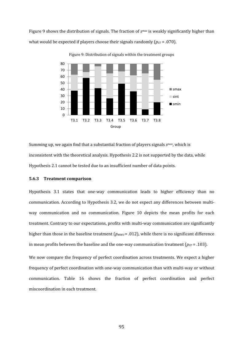
95

Figure 9 shows the distribution of signals. The fraction of smax is weakly significantly higher than

what would be expected if players choose their signals randomly (pST = .070).

Figure 9: Distribution of signals within the treatment groups

Summing up, we again find that a substantial fraction of players signals smax, which is

inconsistent with the theoretical analysis. Hypothesis 2.2 is not supported by the data, while

Hypothesis 2.1 cannot be tested due to an insufficient number of data points.

5.6.3 Treatment comparison

Hypothesis 3.1 states that one-way communication leads to higher efficiency than no

communication. According to Hypothesis 3.2, we do not expect any differences between multi-

way communication and no communication. Figure 10 depicts the mean profits for each

treatment. Contrary to our expectations, profits with multi-way communication are significantly

higher than those in the baseline treatment (pMWU = .012), while there is no significant difference

in mean profits between the baseline and the one-way communication treatment (pFP = .103).

We now compare the frequency of perfect coordination across treatments. We expect a higher

frequency of perfect coordination with one-way communication than with multi-way or without

communication. Table 16 shows the fraction of perfect coordination and perfect

miscoordination in each treatment.

0

10

20

30

40

50

60

70

80

T3.1 T3.2 T3.3 T3.4 T3.5 T3.6 T3.7 T3.8

Group

smax

sint

smin

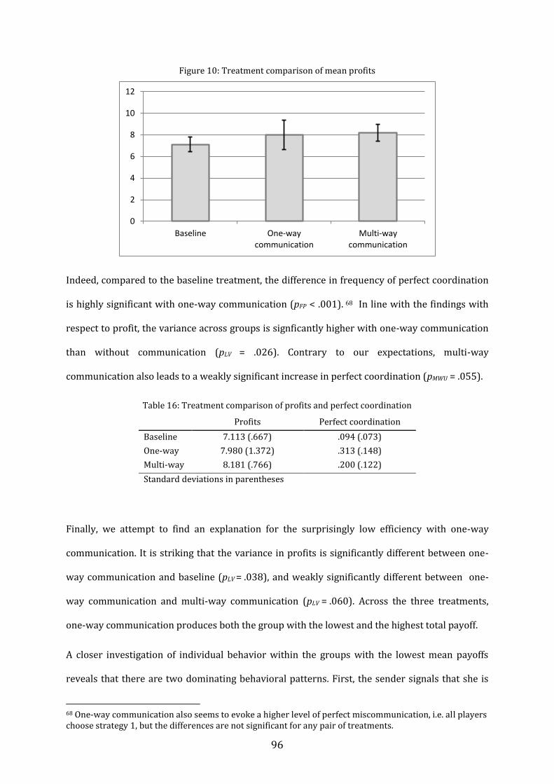
96

Figure 10: Treatment comparison of mean profits

Indeed, compared to the baseline treatment, the difference in frequency of perfect coordination

is highly significant with one-way communication (pFP < .001). 68 In line with the findings with

respect to profit, the variance across groups is signficantly higher with one-way communication

than without communication (pLV = .026). Contrary to our expectations, multi-way

communication also leads to a weakly significant increase in perfect coordination (pMWU = .055).

Table 16: Treatment comparison of profits and perfect coordination

Profits Perfect coordination

Baseline 7.113 (.667) .094 (.073)

One-way 7.980 (1.372) .313 (.148)

Multi-way 8.181 (.766) .200 (.122)

Standard deviations in parentheses

Finally, we attempt to find an explanation for the surprisingly low efficiency with one-way

communication. It is striking that the variance in profits is significantly different between one-

way communication and baseline (pLV = .038), and weakly significantly different between one-

way communication and multi-way communication (pLV = .060). Across the three treatments,

one-way communication produces both the group with the lowest and the highest total payoff.

A closer investigation of individual behavior within the groups with the lowest mean payoffs

reveals that there are two dominating behavioral patterns. First, the sender signals that she is

68 One-way communication also seems to evoke a higher level of perfect miscommunication, i.e. all players choose strategy 1, but the differences are not significant for any pair of treatments.

0

2

4

6

8

10

12

Baseline One-way communication

Multi-way communication

97

not willing to be the hero; second, she signals that she is willing to be the hero, but retreats

afterwards. While the first pattern is fully rational, the second presents a puzzle: from a

theoretical point of view, signaling smax should always be succeeded by choosing effort emax.69

Although the average payoff decreases to 4.64 ECU on average compared to 7.00 ECU if smax was

played, we do not find any sign for learning either. Beyond the question why this behavior

occurs at all, there is a noticeable accumulation within the same groups.70 Thus, an explanation

might be that this unconstructive behavior is perceived as an act of hostility by the remaining

group members, who react by choosing the same signal or pattern for reasons of reciprocity.

This notion is supported by our finding that there is a high correlation between the signal sent in

the last period and the recent signals (Spearman’s rho = .492, p < .001).71

In summary, we do not find clear support for Hypothesis 3.1 that one-way communication

increases efficiency compared to the baseline treatment. Multi-way communication significantly

increases total payoff, which is inconsistent with Hypothesis 3.2.

5.7 Efficiency concerns in the hero game

Although the standard theoretical analyses predict that smax would never be chosen in any of the

two communication regimes, we find that a substantial fraction of subjects send smax. In the

following, we will propose efficiency concerns as an explanatory approach.

There is a large body of evidence showing that people do not only take their individual profits

into account, but also consider the profits of others.72 A number of motives for other-regarding

behavior have been identified, such as inequity aversion, altruism or preferences for efficiency,

the relative importance of which is still subject of discussions.73 We argue that the most

69 This prediction is independent of the player being purely selfish or having efficiency concerns, which we will discuss in more detail in section 5.7. 70 An obvious explanation would be that the same irrational subject is repeatedly chosen to be the sender. Indeed, 3 of the 16 subjects in the affected groups are responsible for 50 % of the deviations from realized signals smax in these groups; however, a total of 8 out of 15 senders shows this behavior. 71 See Table 23 containing mean profits, signals sent and absolute deviations from signal in Appendix A. 72 For an overview, see e.g. Fehr et al. (2006). 73 Altruism means that a person’s utility increases in the outcome of others. In the context discussed here, altruism and preferences for efficiency lead to the same behavior. Inequity aversion (Bolton and Ockenfels 2000, Fehr and Schmidt 1999) refers to disutility caused by the unfairness of outcomes and is reflected by the willingness to bear costs in order to reduce inequality. In the context of the hero game, however,

98

prominent flaw in the hero game is coordination failure resulting in efficiency losses, and that

the dominating non-selfish concern is directed towards the avoidance of these losses. We

account for efficiency concerns by applying the model of quasi-maximin preferences by

Charness and Rabin (2002) to the hero game. In their model, individual utility equals the

weighted sum of one’s own monetary payoff and a social welfare function, which is determined

by the minimum outcome across all players and the total sum of all outcomes

in the group:

with

The weighting parameter γ measures the degree to which the payoffs of others are taken into

account; a purely selfish profit-maximizer is defined by γ = 0. Parameter δ measures the relative

importance of the minimum outcome compared to the aggregated outcomes of all players.

Rawlesian inequity aversion is represented by δ = 1, which means that a person has a particular

interest in increasing the income of the worst-off player, while δ = 0 corresponds to a preference

for maximizing total surplus regardless of its distribution among the players. As we focus on the

effect of efficiency concerns, we assume that δ = 0 and disregard any distributional

considerations. The utility function reduces to

Before analyzing the effects of efficiency concerns in the different communication regimes, we

investigate how a preference for efficiency influences the probability to choose the hero strategy

emax in the mixed strategy equilibrium. We assume that players are symmetric and exhibit the

outcomes are almost necessarily unequal, so players’ opportunities to reveal fairness concerns are very limited. With communication, subjects might attempt to achieve a more equal outcome by deliberately sending deceptive messages; in particular, an envious sender might announce smin although she plans to play strategy emax. However, this behavior is rarely ever observed. Sending smin and playing emax occured three times, which equals 5.17 % of the cases in which the sender sent smin, or 1.88 % of total actions.

99

same degree of preferences for efficiency. We denote the probability to choose the hero strategy

emax by q.74

Statement 5. If all players exhibit the same degree of efficiency concerns, the

probability to choose emax in the symmetric mixed strategy equilibrium is higher than

without efficiency concerns.

The probability q to choose emax in the symmetric mixed strategy equilibrium is

with p being the probability of choosing strategy emax in the mixed strategy equilibrium without

preferences for efficiency.75 Probability q increases in the degree of concern for efficiency.

5.7.1 One-way communication

A selfish player can credibly signal emax and emin, but does not have an incentive to signal and

choose emax, since (smin, emin) yields a higher expected payoff. If only the randomly determined

sender has preferences for efficiency, the sender will choose (smax, emax) if her efficiency

parameter exceeds a certain threshold.76 If all players exhibit efficiency concerns, however, an

increase in not only increases the utility from the payoff of the remaining players, but also the

probability that the remaining players choose the hero strategy in the asymmetric mixed

strategy equilibrium, leading to a higher expected value of choosing (smin, emin). It is therefore not

obvious whether the sender’s behavior will change if all subjects have preferences for efficiency.

In the following, we will show that this is indeed the case.

Statement 6. If all subjects exhibit identical efficiency concerns , the sender will

choose (smax, emax) if exceeds a threshold .

74 As in the underlying game, only strategies emax and emin can be best replies. Let e(1) be the highest effort chosen by all players in the group except for player i. If effort ei exceeds e(1), an increase in effort increases both individual and overall payoff, so player i’s best response is to choose the highest available effort emax. If player i chooses effort ei lower or equal to e(1), decreasing ei increases individual payoff while the payoffs of all other players are not affected, which means that player i’s best response is to choose the lowest available payoff emin. 75 The proof is relegated to Appendix B, p. 121. 76 Since the (expected) payoffs of all players are unaffected by the sender’s , only influences the relative utility of individual and overall payoff; the overall payoff is higher after (smax,emax).

100

We start with the interpretation of messages in the respective subgames. We use the same

mapping of signals into effort choices as before, substituting probability p by q, as shown in

Table 17.

Table 17: Mapping of signals into effort choices

Signaling stage Effort choice stage

smax (emax, emin, …, emin)

sint (qemax, qemax, …, qemax)

smin (emin, q’emax, …, q’emax)

After signaling smax, the sender plays emax and everyone else plays emin. If the sender announces a

strategy sint, s.t. smin < sint < smax, all players including herself play the mixed-strategy Nash

equilibrium where emax is chosen with probability q. Sending smin results in the sender playing

emin while the remaining players choose emax with probability q’ > q.77 Each combination of effort

choices described is an equilibrium in the respective subgame.78

For the following analysis of the two-stage game, we denote the potential outcomes as F

(freeriding), H (hero) and M (miscoordination), respectively, with F > H > M.

refers to the hero outcome resulting from playing emax. Choosing emin leads

to successful freeriding and a payoff if at least one other player chooses the

hero strategy emax, and yields the minimum outcome if all players choose

emin.

To determine the equilibrium of the two-stage game, we compare the (expected) utilities in the

subgames. We denote the (expected) utility of the sender in the subgame equilibrium following a

signal si as Ui and EUi, respectively.

The utility of being the hero in a pure strategy equilibrium following the announcement

smax is given by

77 Analogous to p’, q’ equals the probability to choose strategy emax in an asymmetric mixed strategy equilibrium when all players have preferences for efficiency. 78 (emin, q’emax, q’emax, q’emax) is an equilibrium for .

101

The expected utility in the mixed strategy equilibrium is independent of the sender’s

strategy choice and can therefore be written as

which is strictly smaller than for any

The expected utility of signaling smin and choosing emin, which results in the remaining

players choosing emax with probability , is given by

We set and solve for Given the parameterization in the experiment, utility

is higher than if the efficiency parameter exceeds a threshold .79 It

follows that for , the equilibrium of the two-stage game is equal to the one without

efficiency concerns: the sender signals and chooses emin while the remaining players choose emax

with probability q’. For , however, in equilibrium, the sender signals and chooses emax

while the remaining players choose emin, resulting in perfect coordination on the pure strategy

equilibrium. Since smax and smin lead to Nash equilibria, both signals are self-committing.

Moreover, the signals are self-signaling. The reasoning is analogous to the case without

efficiency concerns, the only difference being that sending smax is now strictly preferred over

sending smin if the sender wants to choose emax. ∎

Without knowledge of the value of the parameter , neither one of the equilibria can be ruled out

on the basis of efficiency concerns. Assuming that exceeds , efficiency concerns thus serve as

an explanation for the observation that signal smax is frequently chosen. One-way communication

allows players to fully solve the coordination problem at low individual costs, thereby triggering

pro-social behavior if players exhibit preferences for efficiency.

79 This means that a player chooses emax if the aggregated profits of the remaining players account for more than approximately 20 % of her utility.

102

5.7.2 Multi-way communication

Assuming that all players believe that messages truthfully indicate actions, there is no mixed

strategy equilibrium of the two-stage game in which strategy smax is sent with positive

probability in the communication stage. This result changes if efficiency concerns are taken into

account.

Statement 7. If all subjects exhibit identical efficiency concerns , signal smax will be

sent with positive probability in a mixed strategy equilibrium.

Being the hero in a pure strategy equilibrium is strictly preferred over a mixed strategy

equilibrium, as shown in the discussion of one-way communication above. Still, being the

freerider in a pure strategy equilibrium is preferred over being the hero for

Table 18: Signaling strategies and resulting utility for player i with efficiency concerns

Utility player i Highest signal of players j ≠i

smax smin

si smax

smin

With regard to the mapping of signals into efforts we assume that, if the effort choices

corresponding to the players’ signals constitute an equilibrium in the following subgame,

players choose the efforts they have announced; otherwise, they ignore the messages sent and

choose effort level emax with probability q. The utilities of the two-stage game resulting from this

mapping are shown in Table 18, with

denoting player i’s (expected) utility from

outcome k. Since

, sending smax and choosing emax is played with positive

probability in a mixed strategy equilibrium of the two-stage game.80 ∎

Moreover, subjects might also have an incentive to send intermediary signals to facilitate

coordination. We will discuss this notion in detail in the next section.

80 For player i to be indifferent between strategies smin and smax, at least one player j ≠i must choose smax with positive probability p. This means that all players except player j are indifferent between strategies smin and smax. It follows that, if all players choose smax with probability p, all players are indifferent between strategy smin and smax.

103

5.8 Intermediary signals as coordination device in the multi-way

communication treatment

5.8.1 Hypotheses

Figure 9 shows that there is a high fraction of intermediary signals in the multi-way

communication treatment. We argue that this might be the case because these signals are used

as a means to improve coordination. In the following, we describe the functioning of this

coordination device, and present a simplified example to illustrate that, under the assumption of

preferences for efficiency, subjects can have incentives to use this device.

Cooper et al. (1989) show theoretically and experimentally that coordination can be improved if

subjects, in addition to being able to announce their future strategy choice, have the option not

to send any message at all. Not sending is considered to be an offer to follow the suggestion of

the second player.81 In the hero game described here, subjects do not have the possibility to not

send a signal. We argue, however, that signaling intermediary strategies serves a similar

purpose as refraining from sending: subjects can use intermediary signals to indicate their

general willingness to exert effort if no one else does so, thereby introducing an element that is

similar to a conditional choice.82 Choosing a random signal increases the probability that exactly

one player sends the highest signal. This establishes a focal point indicating which player is

going to be the hero. As discussed for the case of one-way communication, subjects can thus

choose to be the hero while avoiding the risk of efficiency losses due to other players doing the

same.

Statement 8. Under the assumption of preferences for efficiency, subjects can have

incentives to use intermediary signals as a coordination device.

81 Intuitively, the reasoning is as follows: giving subjects the opportunity not to send a message adds a self-committing strategy to the strategy space, and as this message indicates an action conditional on the messages of others, the game gets a sequential character which improves coordination. For a detailed explanation see Cooper et al. (1989), pp. 569 – 572. Indeed, they find that a large fraction of participants decides not to announce a strategy; with two-way communication, the option not to signal is chosen in 27 % of the cases. 82 This means that we drop the assumption that signal sk is understood as “the sender of this message intends to choose ek”.

104

We proceed with a numerical example. For the sake of clarity, we consider a two-person game

with three effort levels , three corresponding signals and as

before, the profit is given by The utilities resulting

from the effort choices are given by the numerical values are shown in

Table 19. The symmetric mixed strategy equilibrium of the effort stage subgame is

.83

Table 19: Utilities in the reduced effort stage

emax = 7 eint = 4 emin = 1

emax = 7 12, 13.5

eint = 4 13.5, 12 6, 6 7.5, 9

emin = 1 16.5, 13.5 9, 7.5 1.5, 1.5

Adapting the approach by Cooper et al. (1989), we assume that subjects implicitely agree that

the player who sent the unique highest signal chooses emax in the effort choice stage, while the

other player chooses emin. If both players send the same signal, the mixed strategy equilibrium is

played in the effort choice stage, leading to an expected utility of 11.5. This mapping of signals

into efforts leads to the utilities in the two-stage game depicted in Table 20.

The two-stage game has a symmetric mixed-strategy equilibrium in which all three signals are

sent with positive probability.84 The respective probabilities are

and the resulting expected utility is 13.30, while the expected utility of the

babbling equilibrium is 11.5. ∎

83 For the computation of probability q see p. 108. We focus on mixed strategy equilibria; the game also has two equilibria in pure strategies,

with

84 There are also four equilibria in pure strategies:

105

Table 20: Utilities in the reduced two-stage game

smax = 7 sint = 4 smin = 1

smax = 7 11.5, 11.5

sint = 4 16.5, 13.5 11.5, 11.5

smin = 1 16.5, 13.5 16.5, 13.5 11.5, 11.5

We state several hypotheses to test whether the data indicates that the kind of behavioral

pattern we assumed here indeed occurs in the experiment.

Hypothesis 4.1. The fraction of intermediary signals is higher than the fraction of

intermediary effort choices.

Hypothesis 4.2. Players who send a unique maximum signal exert a higher effort than

the remaining players.

Hypothesis 4.3. Players who send a unique maximum signal adjust upwards, i.e. the

chosen effort level is higher than the signal, while the remaining players adjust

downwards.

Hypothesis 4.4. Efforts are better coordinated than signals.

5.8.2 Results

The use of intermediary signals as a coordination device would result in a decrease in choices of

intermediary effort levels compared to the choices in the signaling stage. Indeed, we find a

significant decrease from 37.81 % in the signaling stage to 22.66 % in the effort choice stage

(pWSR = .014), supporting Hypothesis 4.1. Players deviate from their signals in 69.08 % of the

time after sending an intermediary signal, while devations occur only in 21.57 % of the cases if

signals smax or smin were chosen (pWSR = .012).

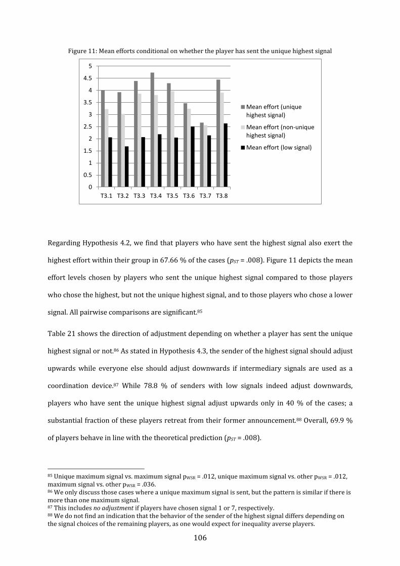
106

Figure 11: Mean efforts conditional on whether the player has sent the unique highest signal

Regarding Hypothesis 4.2, we find that players who have sent the highest signal also exert the

highest effort within their group in 67.66 % of the cases (pST = .008). Figure 11 depicts the mean

effort levels chosen by players who sent the unique highest signal compared to those players

who chose the highest, but not the unique highest signal, and to those players who chose a lower

signal. All pairwise comparisons are significant.85

Table 21 shows the direction of adjustment depending on whether a player has sent the unique

highest signal or not.86 As stated in Hypothesis 4.3, the sender of the highest signal should adjust

upwards while everyone else should adjust downwards if intermediary signals are used as a

coordination device.87 While 78.8 % of senders with low signals indeed adjust downwards,

players who have sent the unique highest signal adjust upwards only in 40 % of the cases; a

substantial fraction of these players retreat from their former announcement.88 Overall, 69.9 %

of players behave in line with the theoretical prediction (pST = .008).

85 Unique maximum signal vs. maximum signal pWSR = .012, unique maximum signal vs. other pWSR = .012, maximum signal vs. other pWSR = .036. 86 We only discuss those cases where a unique maximum signal is sent, but the pattern is similar if there is more than one maximum signal. 87 This includes no adjustment if players have chosen signal 1 or 7, respectively. 88 We do not find an indication that the behavior of the sender of the highest signal differs depending on the signal choices of the remaining players, as one would expect for inequality averse players.

0

0.5

1

1.5

2

2.5

3

3.5

4

4.5

5

T3.1 T3.2 T3.3 T3.4 T3.5 T3.6 T3.7 T3.8

Mean effort (unique highest signal)

Mean effort (non-unique highest signal)

Mean effort (low signal)

107

Table 21: Direction of adjustment

Player sends highest signal Player does not send highest signal adjustment signal = 7 signal < 7 signal = 1 signal > 1 upwards 11 30 11 none 33 6 174 29 downwards 32 28 86 Bold print: in line with the hypothesis

However, this is not reflected in coordination success as stated in Hypothesis 4.4; the difference

between virtual profits based on signals, i.e. those profits that would have been achieved if

players’ efforts were equal to their signals, and realized profits in the effort stage (see Table 22)

is insignificant.

Table 22: Mean profits and efforts with multi-way communication

Mean (virtual) profit Mean (virtual) effort Effort stage (T3) 8.181 (.766) 2.494 (.263) Signaling stage (T3) 8.055 (.945) 3.295 (1.008) Baseline treatment (T1) 7.133 (.667) 2.388 (.209)

Standard deviations in parentheses

There is, however, a significant difference between virtual profits and profits in the baseline

treatment (pMWU = .036); signals sent with multi-way communication are better coordinated than

efforts chosen without communication. The improvement can partly be explained by the fact

that signaled efforts are weakly significantly higher than effort choices in the baseline treatment

(pMWU = .074). 89 This suggests that the players’ willingness to exert a high effort without

communication is lower than their willingness to send a high signal.

To sum up, we find mixed evidence regarding the use of intermediary signals as a coordination

device. Our analysis suggests that there are two effects that interact: analogous to one-way

communication, the opportunity to send a signal triggers an announcement that is higher than

the effort that would have been chosen otherwise; combined with the players’ general

propensity to stick to their announcements and with the coordinating properties of the signals,

multi-way communication thus leads to a significant improvement in efficiency.

89 Figure 12 in the appendix depicts the distribution of efforts and signals.

108

5.9 Conclusion

We test whether communication leads to improved coordination in a game in which the socially

optimal outcome is achieved if exactly one player volunteers at the cost of being relatively worse

off than the remaining players. For one-way communication, standard theory suggests that

senders announce and play the minimum effort, which leads to a slight improvement in terms of

efficiency. For multi-way communication, standard theory predicts no change at all.

In an experimental test we find that, contrary to our expectations, a substantial fraction of

senders in the one-way communication treatment announce and play the maximum effort.

Multi-way communication leads to a significant improvement in efficiency, which again

contradicts standard theoretical predictions. Accounting for preferences for efficiency improves

the explanative power of the theory to a substantial extent, thus providing evidence for the

relevance of social preferences in strategic decision-making.

We attribute the improvement in efficiency that is achieved with multi-way communication to a

higher willingness to exert effort if efficiency losses due to others’ heroic actions can be ruled

out, and to the use of intermediary signals as a coordination device. In contrast to multi-way

communication, one-way communication has the theoretical advantage of enabling the sender of

the message to fully solve the coordination problem. However, the fact that the outcome of the

game depends crucially on the actions of a single player leads to high variability in coordination

success and resulting profits. If the randomly chosen sender exhibits preferences for efficiency,

she can achieve perfect coordination; if her efficiency concerns are less pronounced, or if she

announces that she will play the hero strategy but retreats afterwards, this may lead to results

that are even worse than without communication.

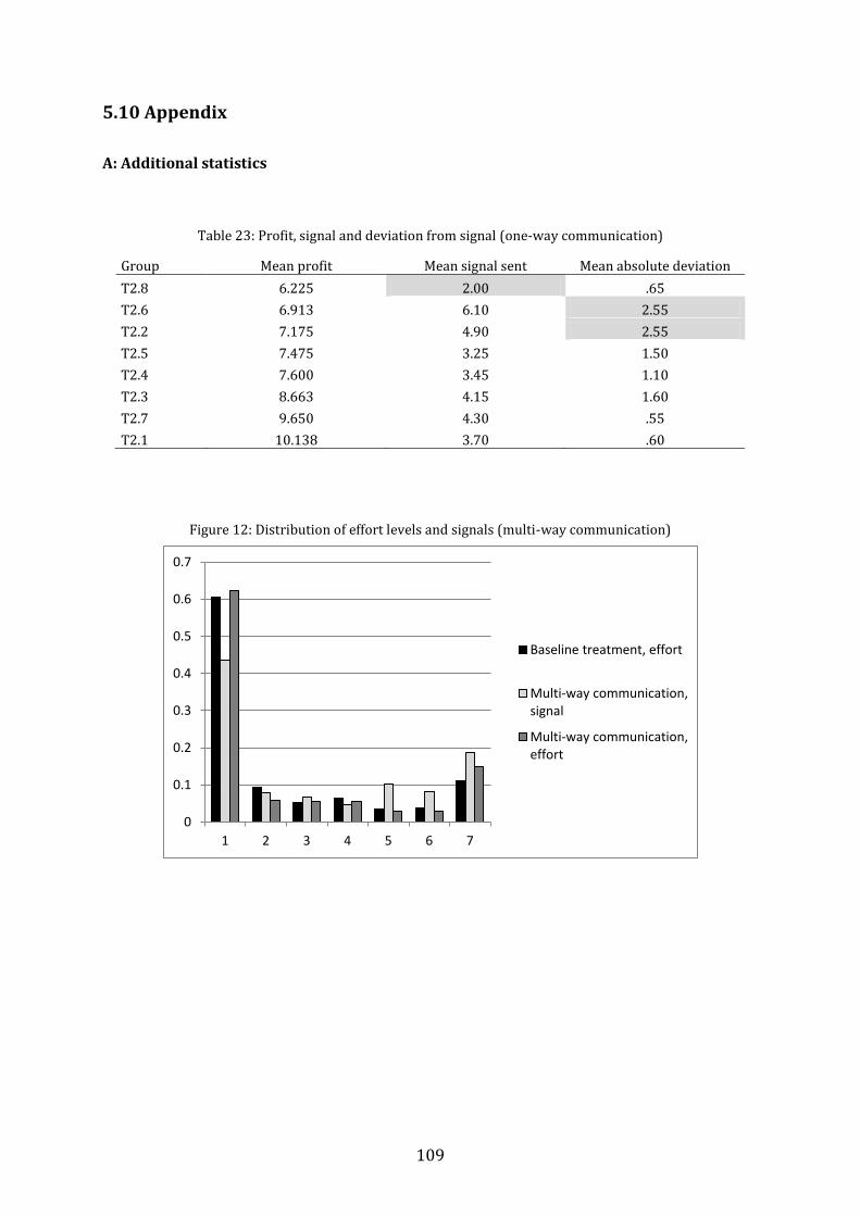
109

5.10 Appendix

A: Additional statistics

Table 23: Profit, signal and deviation from signal (one-way communication)

Group Mean profit Mean signal sent Mean absolute deviation

T2.8 6.225 2.00 .65

T2.6 6.913 6.10 2.55

T2.2 7.175 4.90 2.55

T2.5 7.475 3.25 1.50

T2.4 7.600 3.45 1.10

T2.3 8.663 4.15 1.60

T2.7 9.650 4.30 .55

T2.1 10.138 3.70 .60

Figure 12: Distribution of effort levels and signals (multi-way communication)

0

0.1

0.2

0.3

0.4

0.5

0.6

0.7

1 2 3 4 5 6 7

Baseline treatment, effort

Multi-way communication, signal

Multi-way communication, effort

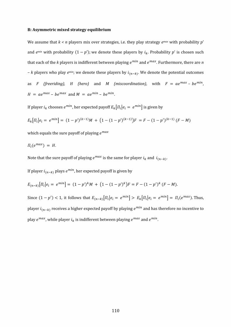
110

B: Asymmetric mixed strategy equilibrium

We assume that k < n players mix over strategies, i.e. they play strategy emax with probability

and emin with probability we denote these players by . Probability is chosen such

that each of the k players is indifferent between playing and . Furthermore, there are n

– k players who play emin; we denote these players by We denote the potential outcomes

as F (freeriding), H (hero) and M (miscoordination), with ,

and

If player chooses , her expected payoff is given by

which equals the sure payoff of playing

Note that the sure payoff of playing is the same for player and

If player plays , her expected payoff is given by

Since , it follows that Thus,

player receives a higher expected payoff by playing and has therefore no incentive to

play while player is indifferent between playing and

111

C: Mixed strategy equilibrium with symmetric efficiency concerns

Again, we denote the potential outcomes as F (freeriding), H (hero) and M (miscoordination),

with , and In a symmetric

mixed strategy equilibrium, probability q is chosen such that the expected utility of choosing emin

equals the expected utility of choosing emax:

. (1)

The expected utility of choosing strategy is given by

the expected utility of choosing strategy is given by

i

with

Note that the expected total outcome of the n – 1 remaining players differs only in case that none

of these players chooses the hero strategy ; in any other case, the expected outcome is

equal ( . Substituting the expected utilities in (1) and solving for q yields

112

Substituting L, H, and F by the underlying payoffs yields

113

D.1: Instructions one-way communication treatment T2 (translation from German)

Welcome and thank you for participating in this experiment. Please do not communicate with

other participants from now on until the end of the experiment. Noncompliance with this rule

will lead to your exclusion from the experiment.

Please read these instructions thoroughly. Please raise your hand should you have any questions

while reading the instructions or during the experiment. One of the experimenters will then

come to you and answer your question. Your payoff as well as your decisions in the experiment

are kept confidential. Participants will not know with whom they interacted during the

experiment, neither during nor after the experiment.

You can earn money during this experiment. How much money you earn depends on your own

decisions as well as on the decisions of the other participants. During the experiment your

payoffs are calculated in a virtual currency, the so called experimental currency units (ECU). 1

ECU is equal to 0.08 Euros. At the end of the experiment your payoffs will be converted into Euro

and paid out to you in cash. Additionally, you receive 2.50 Euro for your appearance.

Before the experiment starts, we will run a short test to check whether you understood the

instructions. All participants have received the same instructions.

Experiment

In this experiment, you will have to take decisions in ten consecutive rounds. In each round you

will form a group with three other participants. This group is matched randomly at the

beginning of each round.

In each round, each participant chooses a number. Possible numbers are 1, 2, 3, 4, 5, 6, and 7.

The highest number of all participants within a group, including your own number, dictates the

potential payoffs.

Your payoff in each round (based on your own decision as well as the decisions of the other

members of your group) is shown in the following table:

114

Your payoff

Highest number within your group Your number 7 6 5 4 3 2 1 7 7.00 – – – – – – 6 8.00 6.00 – – – – – 5 9.00 7.00 5.00 – – – – 4 10.00 8.00 6.00 4.00 – – – 3 11.00 9.00 7.00 5.00 3.00 – – 2 12.00 10.00 8.00 6.00 4.00 2.00 – 1 13.00 11.00 9.00 7.00 5.00 3.00 1.00

The left column represents the number you have chosen, while the upper row indicates the

highest number within your group (including your own number). The payoffs can be found in

the row with the number you have chosen and the column with the highest number within your

group (including your own number).

Every round consists of two stages, the communication stage and the decision stage.

Communication stage. In the communication stage one member of your group is randomly

chosen as sender. The sender sends a message to the other members of her group, in which she

can inform the others which number she intends to choose. Possible messages are the numbers

1 to 7. We ask you to let us know in every communication stage which message you wish to

send, if you are randomly chosen to be sender.

Decision stage. In the decision stage you will be informed if you are the sender and which

number the sernder has sent. Afterwards, you choose your number for the decision.

Apart from choosing your own number within each round, we ask you to estimate the highest

number of your entire group (including your own number).

115

After each round you will be able to see your own number, the highest number of your group

and your payoff from the respective round. Afterwards the next round begins.

At the end of all ten rounds, your payoffs are summed up, converted into Euro and displayed on

your screen together with the 2.50 Euro for your appearance. Finally, you will receive a

questionnaire, which we ask you to complete while the payments are prepared.

In every round you therefore need to make three entries:

Communication stage:

The message you wish to send if you are the sender

Decision stage: After being informed, whether you are the sender and which number has been sent:

Your number

Your expectation about which number (including your own number) is the highest number

chosen in your group

116

D.2: Instructions multi-way communication treatment T3 (Translation from German)

Welcome and thank you for participating in this experiment. Please do not communicate with

other participants from now on until the end of the experiment. Noncompliance with this rule

will lead to your exclusion from the experiment.

Please read these instructions thoroughly. Please raise your hand should you have any questions

while reading the instructions or during the experiment. One of the experimenters will then

come to you and answer your question. Your payoff as well as your decisions in the experiment

are kept confidential. Participants will not know with whom they interacted during the

experiment, neither during nor after the experiment.

You can earn money during this experiment. How much money you earn depends on your own

decisions as well as on the decisions of the other participants. During the experiment your

payoffs are calculated in a virtual currency, the so called experimental currency units (ECU). 1

ECU is equal to 0.08 Euros. At the end of the experiment your payoffs will be converted into Euro

and paid out to you in cash. Additionally, you receive 2.50 Euro for your appearance.

Before the experiment starts, we will run a short test to check whether you understood the

instructions. All participants have received the same instructions.

Experiment

In this experiment, you will have to take decisions in ten consecutive rounds. In each round you

will form a group with three other participants. This group is matched randomly at the

beginning of each round.

In each round, each participant chooses a number. Possible numbers are 1, 2, 3, 4, 5, 6, and 7.

The highest number of all participants within a group, including your own number, dictates the

potential payoffs.

Your payoff in each round (based on your own decision as well as the decisions of the other

members of your group) is shown in the following table:

117

Your payoff

Highest number within your group Your number 7 6 5 4 3 2 1 7 7.00 – – – – – – 6 8.00 6.00 – – – – – 5 9.00 7.00 5.00 – – – – 4 10.00 8.00 6.00 4.00 – – – 3 11.00 9.00 7.00 5.00 3.00 – – 2 12.00 10.00 8.00 6.00 4.00 2.00 – 1 13.00 11.00 9.00 7.00 5.00 3.00 1.00

The left column represents the number you have chosen, while the upper row indicates the

highest number within your group (including your own number). The payoffs can be found in

the row with the number you have chosen and the column with the highest number within your

group (including your own number).

Every round consists of two stages, the communication stage and the decision stage.

Communication stage. In the communication stage you send a message to the members of your

group, in which you can inform the others which number you intend to choose. Possible

messages are the numbers 1 to 7.

Decision stage. In the decision stage you will be informed which number the other members of

your group have sent. Afterwards, you choose your number for the decision.

Apart from choosing your own number within each round, we ask you to estimate the highest

number of your entire group (including your own number).

In every round you therefore need to make three entries:

Communication stage:

Your message

Decision stage: After being informed which numbers have been sent:

Your number

Your expectation about which number (including your own number) is the highest number

chosen in your group

118

After each round you will be able to see your own number, the highest number of your group

and your payoff from the respective round. Afterwards the next round begins.

At the end of all ten rounds, your payoffs are summed up, converted into Euro and displayed on

your screen together with the 2.50 Euro for your appearance. Finally, you will receive a

questionnaire, which we ask you to complete while the payments are prepared.

119

6 Conclusion

This thesis consists of four experimental studies that investigate human behavior under risk and

uncertainty in different settings. While the first two studies deal with risky decision-making of a

single person, the third and fourth study are concerned with strategic interaction. In the first

paper, we show that individuals hold systematically wrong beliefs about their success

probabilities in a given task. Nonetheless, we find that the average belief on the population level

is quite accurate. In the second paper, we show that a number of individuals change their risk-

taking behavior if their decisions additionally affect a second, passive party, and that they are

influenced by the decisions of others, whereas standard theory predicts that none of these

factors should have any effect. In the strategic setting in the third paper, we find that standard

theory predicts actual behavior in the experiment fairly well; yet, we find that a substantial

number of subjects repeatedly chooses strategies that should never be chosen according to

standard theory. Finally, in the fourth study, we show that accounting for preferences for

efficiency allows for a better organization of our data than standard theory alone. Our studies

thus contribute to the field of behavioral economics by demonstrating the importance of

integrating behavioral factors into the theoretical modeling to derive more precise predictions

for actual human choice behavior under risk and uncertainty.

120

7 References

Abdellaoui, M., B. Aurelien, P. Laetitia and P. W. Peter (2011). The rich domain of uncertainty: Source functions and their experimental implementation. American Economic Review 101(2): 695-723.

Abdellaoui, M., F. Vossmann and M. Weber (2005). Choice-based elicitation and decomposition of decision weights for gains and losses under uncertainty. Management Science 51(9): 1384-1399.

Aumann, R. J. (1990). Nash equilibria are not self-enforcing. In: Economic decision-making: Games, econometrics and optimization. J. J. Gabszewicz, J.-F. Richard and L. A. Wolsey. Amsterdam, Elsevier.

Baker, R. J., S. K. Laury and A. W. Williams (2008). Comparing small-group and individual behavior in lottery-choice experiments. Southern Economic Journal 75(2): 367-382.

Baliga, S. and S. Morris (2002). Coordination, spillovers, and cheap talk. Journal of Economic Theory 105(2): 450-468.

Baumann, A. O., R. B. Deber and G. G. Thompson (1991). Overconfidence among physicians and nurses: The 'micro-certainty, macro-uncertainty' phenomenon. Social Science & Medicine 32(2): 167-174.

Bereby-Meyer, Y. and A. E. Roth (2006). The speed of learning in noisy games: Partial reinforcement and the sustainability of cooperation. American Economic Review 96(4): 1029-1042.

Blavatskyy, P. (2009). Betting on own knowledge: Experimental test of overconfidence. Journal of Risk and Uncertainty 38(1): 39-49.

Blume, A. and A. Ortmann (2007). The effects of costless pre-play communication: Experimental evidence from games with pareto-ranked equilibria. Journal of Economic Theory 132(1): 274-290.

Bohnet, I., F. Greig, B. Herrmann and R. Zeckhauser (2008). Betrayal aversion: Evidence from Brazil, China, Oman, Switzerland, Turkey, and the United States. The American Economic Review 98: 294-310.

Bolton, G. E., J. Brandts and A. Ockenfels (2005). Fair procedures: Evidence from games involving lotteries. The Economic Journal 115.

Bolton, G. E. and A. Ockenfels (2000). ERC: A theory of equity, reciprocity, and competition. The American Economic Review 90(1): 166-193.

Bolton, G. E. and A. Ockenfels (2010). Betrayal aversion: Evidence from Brazil, China, Oman, Switzerland, Turkey, and the United States: Comment. The American Economic Review 100(1): 628-33.

Bolton, G. E., A. Ockenfels and J. Stauf (2012). Risk taking in a social context. Mimeo.

Brandenburger, A. (1996). Strategic and structural uncertainty in games. In: Wise choices: Games, decisions, and negotiations. R. Zeckhauser, R. Keeney and J. Sibenius. Boston, Harvard Business School Press: 221–232.

Brennan, G., L. G. González, W. Güth and M. V. Levati (2008). Attitudes toward private and collective risk in individual and strategic choice situations. Journal of Economic Behavior & Organization 67(1): 253-262.

Brenner, L. A., D. J. Koehler, V. Liberman and A. Tversky (1996). Overconfidence in probability and frequency judgments: A critical examination. Organizational Behavior and Human Decision Processes 65(3): 212-219.

121

Budescu, D. V., T. S. Wallsten and W. T. Au (1997). On the importance of random error in the study of probability judgment. Part II: Applying the stochastic judgment model to detect systematic trends. Journal of Behavioral Decision Making 10(3): 173-188.

Burton, A. and M. Sefton (2004). Risk, pre-play communication and equilibrium. Games and Economic Behavior 46(1): 23-40.

Camerer, C. (2003). Behavioral game theory: Experiments in strategic interaction. Princeton, Princeton University Press.

Camerer, C. and D. Lovallo (1999). Overconfidence and excess entry: An experimental approach. The American Economic Review 89(1): 306-318.

Camerer, C. F. and G. Loewenstein (2004). Behavioral economics: Past, present, future. In: Advances in behavioral economics. C. F. Camerer, G. Loewenstein and M. Rabin. Princeton, NJ, Princeton University Press: 3 - 51.

Carpenter, J. P. (2002). Information, fairness, and reciprocity in the best shot game. Economics Letters 75(2): 243-248.

Charness, G. (2000). Self-serving cheap talk: A test of aumann's conjecture. Games and Economic Behavior 33(2): 177-194.

Charness, G. and M. O. Jackson (2009). The role of responsibility in strategic risk-taking. Journal of Economic Behavior & Organization 69(3): 241-247.

Charness, G. and M. Rabin (2002). Understanding social preferences with simple tests. The Quarterly Journal of Economics 117(3): 817-869.

Cheng, P. Y. K. (2007). The trader interaction effect on the impact of overconfidence on trading performance: An empirical study. Institutional Investor 2(4): 50-63.

Coelho, M. and D. de Meza (2012). Do bad risks know it? Experimental evidence on optimism and adverse selection. Economics Letters 114(2): 168-171.

Compte, O. and A. Postlewaite (2004). Confidence-enhanced performance. The American Economic Review 94(5): 1536-1557.

Cooper, D. J. and J. H. Kagel (forthcoming). Other regarding preferences: A selective survey of experimental results. In: The handbook of experimental economics vol. 2. J. H. Kagel and A. E. Roth.

Cooper, D. J. and M. Rege (2011). Misery loves company: Social regret and social interaction effects in choices under risk and uncertainty. Games and Economic Behavior 73(1): 91-110.

Cooper, R., D. V. DeJong, R. Forsythe and T. W. Ross (1989). Communication in the battle of the sexes game: Some experimental results. The RAND Journal of Economics 20(4): 568-587.

Cooper, R., D. V. DeJong, R. Forsythe and T. W. Ross (1992). Communication in coordination games. The Quarterly Journal of Economics 107(2): 739-771.

Crawford, V. (1998). A survey of experiments on communication via cheap talk. Journal of Economic Theory 78(2): 286-298.

Cummings, Ronald G., S. Elliott, Glenn W. Harrison and J. Murphy (1997). Are hypothetical referenda incentive compatible? Journal of Political Economy 105(3): 609-621.

Daniel, K., D. Hirshleifer and A. Subrahmanyam (1998). Investor psychology and security market under- and overreactions. The Journal of Finance 53(6): 1839-1885.

Darley, J. M. and B. Latané (1968). Bystander intervention in emergencies: Diffusion of responsibility. Journal of Personality and Social Psychology 8(41): 377-383.

Dawes, R. M. (1980). Social dilemmas. Annual Review of Psychology 31(1): 169-193.

122

DellaVigna, S. (2009). Psychology and economics: Evidence from the field. Journal of Economic Literature 47(2): 315-372.

Devetag, G. and A. Ortmann (2007). When and why? A critical survey on coordination failure in the laboratory. Experimental Economics 10(3): 331-344.

Diekmann, A. (1985). Volunteer's dilemma. The Journal of Conflict Resolution 29(4): 605-610.

Diekmann, A. (1986). Volunteer's dilemma. A social trap without a dominant strategy and some empirical results. In: Paradoxical effects of social behavior: Essays in honor of anatol rapoport, Heidelberg and Vienna: Physica: 187-197.

Duffy, J. and N. Feltovich (1999). Does observation of others affect learning in strategic environments? An experimental study. International Journal of Game Theory 28(1): 131-152.

Eberlein, M., S. Ludwig and J. Nafziger (2006). The effects of feedback on self-assessment. Bulletin of Economic Research 63(2): 177-199.

Erev, I., T. S. Wallsten and D. V. Budescu (1994). Simultaneous over- and underconfidence: The role of error in judgment processes. Psychological Review 101(3): 519-527.

Farrell, J. (1987). Cheap talk, coordination, and entry. The RAND Journal of Economics 18(1): 34-39.

Farrell, J. and M. Rabin (1996). Cheap talk. The Journal of Economic Perspectives 10(3): 103-118.

Fehr, E. and K. M. Schmidt (1999). A theory of fairness, competition, and cooperation. The Quarterly Journal of Economics 114(3): 817-868.

Fehr, E. and K. M. Schmidt (2006). The economics of fairness, reciprocity and altruism - experimental evidence and new theories. In: Handbook on the economics of giving, reciprocity and altruism. S.-C. Kolm and J. M. Ythier, Elsevier. Volume 1: 615-691.

Feldhaus, C. (2011). A hero game. Theory and experimental evidence. Wirtschafts- und Sozialwissenschaftliche Fakultät, Universität zu Köln. Diploma thesis.

Feldhaus, C. and J. Stauf (2012). A hero game. Mimeo.

Fellner, G. and S. Krügel (2012). Judgmental overconfidence: Three measures, one bias? Journal of Economic Psychology 33(1): 142-154.

Fischbacher, U. (2007). Z-tree: Zurich toolbox for ready-made economic experiments. Experimental Economics 10(2): 171-178.

Fischhoff, B., P. Slovic and S. Lichtenstein (1977). Knowing with certainty: The appropriateness of extreme confidence. Journal of Experimental Psychology: Human Perception and Performance 3(4): 552-564.

Gibbons, R. (1992). A primer in game theory. New York, Harvester Wheatsleaf.

Greiner, B. (2004). An online recruitment system for economic experiments. In: Forschung und Wissenschaftliches Rechnen 2003. K. Kremer and V. Macho. Goettingen, Gesellschaft für Wissenschaftliche Datenverarbeitung.

Griffin, D. W. and C. A. Varey (1996). Towards a consensus on overconfidence. Organizational Behavior and Human Decision Processes 65(3): 227-231.

Güth, W., M. V. Levati and M. Ploner (2008). On the social dimension of time and risk preferences: An experimental study. Economic Inquiry 46(2): 261-272.

Harrison, G. W. and J. Hirshleifer (1989). An experimental evaluation of weakest link/best shot models of public-goods. Journal of Political Economy 97(1): 201-225.

Heath, C. and A. Tversky (1991). Preference and belief: Ambiguity and competence in choice under uncertainty. Journal of Risk and Uncertainty 4(1): 5-28.

123

Heinemann, F., R. Nagel and P. Ockenfels (2009). Measuring strategic uncertainty in coordination games. Review of Economic Studies 76(1): 40.

Hey, J. D. and J. Lee (2005). Do subjects separate (or are they sophisticated)? Experimental Economics 8(3): 233-265.

Hilton, D., I. Régner, L. Cabantous, L. Charalambides and S. Vautier (2011). Do positive illusions predict overconfidence in judgment? A test using interval production and probability evaluation measures of miscalibration. Journal of Behavioral Decision Making 24(2): 117-139.

Hirshleifer, J. (1983). From weakest-link to best-shot: The voluntary provision of public goods. Public Choice 41(3): 371-386.

Hoelzl, E. and A. Rustichini (2005). Overconfident: Do you put your money on it? The Economic Journal 115(503): 305-318.

Holt, C. A. and S. K. Laury (2002). Risk aversion and incentive effects. The American Economic Review 92(5): 1644-1655.

Juslin, P. and H. Olsson (1997). Thurstonian and brunswikian origins of uncertainty in judgment: A sampling model of confidence in sensory discrimination. Psychological Review 104(2): 344-366.

Juslin, P., A. Winman and H. Olsson (2000). Naive empiricism and dogmatism in confidence research: A critical examination of the hard-easy effect. Psychological Review 107(2): 384-396.

Kagel, J. H. and A. E. Roth (1995). Handbook of experimental economics. Princeton, Princeton University Press.

Karni, E. (2009). A mechanism for eliciting probabilities. Econometrica 77(2): 603-606.

Keh, H. T., M. D. Foo and B. C. Lim (2002). Opportunity evaluation under risky conditions: The cognitive processes of entrepreneurs. Entrepreneurship Theory and Practice 27(2): 125-148.

Kilka, M. and M. Weber (2001). What determines the shape of the probability weighting function under uncertainty? Management Science 47(12): 1712-1726.

Knight, F. H. (1921). Risk, uncertainty and profit. Boston, Houghton Mifflin.

Krawczyk, M. and F. Le Lec (2010). "Give me a chance!" An experiment in social decision under risk. Experimental Economics 13(4): 500-511.

Larrick, R. P., K. A. Burson and J. B. Soll (2007). Social comparison and confidence: When thinking you're better than average predicts overconfidence (and when it does not). Organizational Behavior and Human Decision Processes 102(1): 76-94.

Ledyard, J. O. (1995). Public goods: A survey of experimental research. In: Handbook of Experimental Economics. A. E. Roth and J. H. Kagel. Princeton, Princeton University Press: 111-181.

Lee, J. (2008). The effect of the background risk in a simple chance improving decision model. Journal of Risk and Uncertainty 36(1): 19-41.

Malmendier, U. and G. Tate (2005). Ceo overconfidence and corporate investment. The Journal of Finance 60(6): 2661-2700.

Malmendier, U. and G. Tate (2008). Who makes acquisitions? Ceo overconfidence and the market's reaction. Journal of Financial Economics 89(1): 20-43.

Masclet, D., N. Colombier, L. Denant-Boemont and Y. Lohéac (2009). Group and individual risk preferences: A lottery-choice experiment with self-employed and salaried workers. Journal of Economic Behavior & Organization 70(3): 470-484.

124

Moore, D. A. and P. J. Healy (2008). The trouble with overconfidence. Psychological Review 115(2): 502-517.

Moore, D. A. and T. G. Kim (2003). Myopic social prediction and the solo comparison effect. Journal of Personality and Social Psychology 85(6): 1121-1135.

Ockenfels, A. and R. Selten (2005). Impulse balance equilibrium and feedback in first price auctions. Games and Economic Behavior 51(1): 155-170.

Ockenfels, A., D. Sliwka and P. Werner (2012). Bonus payments and reference point violations. Working Paper.

Offerman, T., J. Sonnemans, G. Van De Kuilen and P. P. Wakker (2009). A truth serum for non-bayesians: Correcting proper scoring rules for risk attitudes. Review of Economic Studies 76(4): 1461-1489.

Pfeifer, P. E. (1994). Are we overconfident in the belief that probability forecasters are overconfident? Organizational Behavior and Human Decision Processes 58(2): 203-213.

Posten, A.-C., A. Ockenfels and T. Mussweiler (2012). How activating cognitive content shapes trust: A subliminal priming study. University of Cologne Working Paper.

Prasnikar, V. and A. E. Roth (1992). Considerations of fairness and strategy - experimental data from sequential games. Quarterly Journal of Economics 107(3): 865-888.

Rasmusen, E. (1989). Games and information: An introduction to game theory. Malden/Oxford, Blackwell Publishers.

Reynolds, D. B., J. Joseph and R. Sherwood (2009). Risky shift versus cautious shift: Determining differences in risk taking between private and public management decision-making. Journal of Business & Economics Research 7(1): 63-77.

Rohde, I. M. T. and K. I. M. Rohde (2011). Risk attitudes in a social context. Journal of Risk and Uncertainty 43: 205-225.

Saha, A. (1993). Expo-power utility: A 'flexible' form for absolute and relative risk aversion. American Journal of Agricultural Economics 75(4): 905-913.

Saito, K. (2012). Social preferences under uncertainty. Equality of opportunities vs. equality of outcome. Working Paper.

Savage, L. J. (1971). Elicitation of personal probabilities and expectations. Journal of the American Statistical Association 66(336): 783-&.

Selten, R. (1967). Die Strategiemethode zur Erforschung des eingeschränkt rationalen Verhaltens im Rahmen eines Oligopolexperiments. Beiträge zur Experimentellen Wirtschaftsforschung: 136-168.

Selten, R. (1998). Axiomatic characterization of the quadratic scoring rule. Experimental Economics 1(1): 43-62.

Selten, R. (1998). Features of experimentally observed bounded rationality. European Economic Review 42(3-5): 413-436.

Selten, R. and R. Stoecker (1986). End behavior in sequences of finite prisoner's dilemma supergames: A learning theory approach. Journal of Economic Behavior and Organization 7(1): 47-70.

Simon, M., S. M. Houghton and K. Aquino (2000). Cognitive biases, risk perception, and venture formation: How individuals decide to start companies. Journal of Business Venturing 15(2): 113-134.

Soll, J. B. (1996). Determinants of overconfidence and miscalibration: The roles of random error and ecological structure. Organizational Behavior and Human Decision Processes 65(2): 117-137.

125

Starmer, C. and R. Sugden (1991). Does the random-lottery incentive system elicit true preferences? An experimental investigation. The American Economic Review 81(4): 971-978.

Stauf, J., D. Urbig and U. Weitzel (2011). What is your level of overconfidence? A strictly incentive compatible measurement method. Mimeo.

Stotz, O. and R. von Nitzsch (2005). The perception of control and the level of overconfidence: Evidence from analyst earnings estimates and price targets. Journal of Behavioral Finance 6(3): 121-128.

Tversky, A. and D. Kahneman (1992). Advances in prospect theory: Cumulative representation of uncertainty. Journal of Risk and Uncertainty 5(4): 297-323.

Van Huyck, J. B., R. C. Battalio and R. O. Beil (1990). Tacit coordination games, strategic uncertainty, and coordination failure. American Economic Review 80(1): 234-248.

Van Huyck, J. B., R. C. Battalio and R. O. Beil (1991). Strategic uncertainty, equilibrium selection, and coordination failure in average opinion games. Quarterly Journal of Economics 106(3): 885-910.

Wakker, P. P. (2004). On the composition of risk preference and belief. Psychological Review 111(1): 236-241.

Wansbeek, T. and E. Meijer (2000). Measurement error and latent variables in econometrics. Advanced Textbooks in Econometrics 37.

Wu, B. and A. M. Knott (2006). Entrepreneurial risk and market entry. Management Science 52(9): 1315-1330.