essays on economic growth in india
TRANSCRIPT

Louisiana State UniversityLSU Digital Commons
LSU Doctoral Dissertations Graduate School
2017
Essays on Economic Growth In IndiaSujana KabirajLouisiana State University and Agricultural and Mechanical College, [email protected]
Follow this and additional works at: https://digitalcommons.lsu.edu/gradschool_dissertations
Part of the Economics Commons
This Dissertation is brought to you for free and open access by the Graduate School at LSU Digital Commons. It has been accepted for inclusion inLSU Doctoral Dissertations by an authorized graduate school editor of LSU Digital Commons. For more information, please [email protected].
Recommended CitationKabiraj, Sujana, "Essays on Economic Growth In India" (2017). LSU Doctoral Dissertations. 4476.https://digitalcommons.lsu.edu/gradschool_dissertations/4476

ESSAYS ON ECONOMIC GROWTH IN INDIA
A Dissertation
Submitted to the Graduate Faculty of theLouisiana State University and
Agricultural and Mechanical Collegein partial fulfillment of the
requirements for the degree ofDoctor of Philosophy
in
The Department of Economics
bySujana Kabiraj
B.A., University of Calcutta, 2008M.A., Delhi School of Economics, 2010M.S., Louisiana State University, 2014
August 2017

Dedicated to Baba, Maa, and Bon
ii

AcknowledgmentsFirst of all, I would like to express my sincere gratitude to Dr. Areendam Chanda,
my advisor, for inspiration and continuous support. It was his encouragement and
optimism combined with great knowledge and insight which got me through the
rigorous academic process. Learning from him is a privilege, and I will always cherish
his motivation without which this dissertation would not have been possible.
I thank Dr. Bulent Unel and Dr. Ozkan Eren for their valuable insights and
encouragements. I am grateful to Dr. Jenny Minier from the University of Kentucky
for providing me with the data for the fourth chapter of this dissertation. I am also
grateful to Dr. Carter Hill, Dr. W. Douglas McMillin, Dr. Seunghwa Rho, and
all other professors in the Economics Department at the Louisiana State University
for their patience in teaching me everything I know. I also thank Professor Charles
Roussel from LSU and Dr. Mausumi Das from Delhi School of Economics for their
continuous support and invaluable advice.
I have found great support from my colleagues, friends, and family during my
time as a doctoral student. I feel truly blessed to have my parents and sister for the
wonderful people they are. I am grateful to Sara, Omer, Masa, Ting, Ishita, Satadru,
Grace and other economics graduate students for their help and support, and my
beloved friends Sayan, Ananya, Arghya, Subhajit, Saikat, Joy, and Trina for being
there through thick and thin. Last but not the least, I would like to thank Arnab
for his constant encouragement and support.
iii

Table of ContentsACKNOWLEDGMENTS . . . . . . . . . . . . . . . . . . . . . . . . . . . . . . . . . . . . . . . . . . . . . . . . . . . iii
ABSTRACT . . . . . . . . . . . . . . . . . . . . . . . . . . . . . . . . . . . . . . . . . . . . . . . . . . . . . . . . . . . . . . . . vi
CHAPTER1 INTRODUCTION . . . . . . . . . . . . . . . . . . . . . . . . . . . . . . . . . . . . . . . . . . . . . . . . . . . 1
2 LOCAL GROWTH AND CONVERGENCE IN IN-DIA (2000-2010) . . . . . . . . . . . . . . . . . . . . . . . . . . . . . . . . . . . . . . . . . . . . . . . . . . . . . 92.1 Introduction . . . . . . . . . . . . . . . . . . . . . . . . . . . . . . . . . . . . . . . . . . . . . . . . . . . . 92.2 Related Works. . . . . . . . . . . . . . . . . . . . . . . . . . . . . . . . . . . . . . . . . . . . . . . . . . 122.3 Data and Empirical Methodology . . . . . . . . . . . . . . . . . . . . . . . . . . . . . . . 152.4 Results . . . . . . . . . . . . . . . . . . . . . . . . . . . . . . . . . . . . . . . . . . . . . . . . . . . . . . . . . 292.5 Public Projects and Rural Growth . . . . . . . . . . . . . . . . . . . . . . . . . . . . . . 482.6 Conclusion . . . . . . . . . . . . . . . . . . . . . . . . . . . . . . . . . . . . . . . . . . . . . . . . . . . . . 56
3 EFFECT OF CREDIT SUPPLY SHOCK ON GROWTH . . . . . . . . . . . . 573.1 Introduction . . . . . . . . . . . . . . . . . . . . . . . . . . . . . . . . . . . . . . . . . . . . . . . . . . . . 573.2 Background . . . . . . . . . . . . . . . . . . . . . . . . . . . . . . . . . . . . . . . . . . . . . . . . . . . . 583.3 Data . . . . . . . . . . . . . . . . . . . . . . . . . . . . . . . . . . . . . . . . . . . . . . . . . . . . . . . . . . . 613.4 Empirical Design . . . . . . . . . . . . . . . . . . . . . . . . . . . . . . . . . . . . . . . . . . . . . . . 663.5 Results . . . . . . . . . . . . . . . . . . . . . . . . . . . . . . . . . . . . . . . . . . . . . . . . . . . . . . . . . 703.6 Conclusion . . . . . . . . . . . . . . . . . . . . . . . . . . . . . . . . . . . . . . . . . . . . . . . . . . . . . 82
4 MEASURING THE EFFECT OF MISALLOCATIONON PRODUCTIVITY IN INDIAN MANUFACTUR-ING: A GROSS OUTPUT APPROACH . . . . . . . . . . . . . . . . . . . . . . . . . . . . . 834.1 Introduction . . . . . . . . . . . . . . . . . . . . . . . . . . . . . . . . . . . . . . . . . . . . . . . . . . . . 834.2 Related Works. . . . . . . . . . . . . . . . . . . . . . . . . . . . . . . . . . . . . . . . . . . . . . . . . . 864.3 Model . . . . . . . . . . . . . . . . . . . . . . . . . . . . . . . . . . . . . . . . . . . . . . . . . . . . . . . . . . 884.4 Data . . . . . . . . . . . . . . . . . . . . . . . . . . . . . . . . . . . . . . . . . . . . . . . . . . . . . . . . . . . 1024.5 Empirical Analysis . . . . . . . . . . . . . . . . . . . . . . . . . . . . . . . . . . . . . . . . . . . . . 1074.6 Misallocation and Firm Size . . . . . . . . . . . . . . . . . . . . . . . . . . . . . . . . . . . . 1184.7 Conclusion . . . . . . . . . . . . . . . . . . . . . . . . . . . . . . . . . . . . . . . . . . . . . . . . . . . . . 119
5 CONCLUDING REMARKS . . . . . . . . . . . . . . . . . . . . . . . . . . . . . . . . . . . . . . . . . 121
iv

REFERENCES . . . . . . . . . . . . . . . . . . . . . . . . . . . . . . . . . . . . . . . . . . . . . . . . . . . . . . . . . . . . . . 123
APPENDIXA DATA DESCRIPTION . . . . . . . . . . . . . . . . . . . . . . . . . . . . . . . . . . . . . . . . . . . . . . 131
VITA . . . . . . . . . . . . . . . . . . . . . . . . . . . . . . . . . . . . . . . . . . . . . . . . . . . . . . . . . . . . . . . . . . . . . . . 135
v

AbstractThis dissertation comprises of three distinct studies that contribute to the field of
economic growth in India. First, we investigate patterns of growth at the district
level (second level administrative units) using radiance calibrated night lights data for
2000-2010. We examine growth both at the aggregated district level, as well as along
the rural and urban dimensions. We find evidence of both absolute and conditional
convergence, with convergence among rural areas being the primary driver. However,
there is no evidence of convergence among urban areas.
Moving further along similar lines, we explore the effect of credit shocks, gener-
ated by scheduled commercial banks, on economic growth in districts of India during
the years 2000-2010. We exploit the variation in the initial sectoral credit shares
to predict the district level credit supply shock using a shift share instrument. We
find a strong association between credit growth and growth in economic activity, but
when controlled for the district specific demand shocks, the predicted supply shock
effect fails to be statistically significant.
Lastly, we study distortions in input and output markets as the sources of mis-
allocation in the Indian manufacturing sector, using data from both formal and
informal firms. We consider output, capital, raw material, energy, and service sector
distortions in a monopolistically competitive framework to measure the aggregate
dispersion in total factor revenue productivity (TFPR). Decomposing the variance
in TFPR, we show that the raw material and output distortions play the major role
in defining aggregate misallocation.
vi

Chapter 1IntroductionEconomic liberalization in 1991 resulted in a dramatic shift in economic policy land-
scape of the Indian economy. The country has experienced substantial growth along
with structural transformation over the last couple of decades. During 1990-2013,
the share of agriculture in total GDP declined from 28.5% to 13.9%, whereas the
total value of services increased from 49% to 67%. This structural transformation
combined with an average annual growth of 6.5% placed India, along with the other
BRIC countries, in the lime light as an “emerging giant” (Panagariya [2008]).
Despite the apparent structural transformation, the majority of the population
in India continues to live in rural areas. Specifically, according to the 2011 census, the
rural share of population was 68%. Additionally, despite the fall in agricultural share
in GDP, almost 72% of the rural population was engaged in agricultural activities.
The rest of the population working outside the agriculture sector are mostly employed
in the unorganized industry or service sector. Employment in the organized sector
has remained stagnant at around 10% of the working population.
Panagariya [2008] has attributed this slow structural transition to the stagnation
in the manufacturing output at 17% as a share of GDP between 1990-2004. He fur-
ther argues that the slower growth in labor intensive organized manufacturing sector
compared to the skilled labor and capital intensive services create the barrier to over-
all structural transition in India and promotes what economists aptly called “jobless
growth” (Subramanian [2009]). This argument becomes more relevant when we look
1

at the growing share of service sector GDP compared to a decline in manufacturing
share to 12% in 2013-14.
The rural-urban “dualism” is further reflected in human capital attainment –
58% of rural population is literate compared to the 74% of the urban population.
In terms of infrastructure, 93% of the households in urban areas had an electricity
connection whereas only 55% of households in rural areas had the same. The unequal
distribution of opportunity across the sectors and regions has become one of the main
concerns for policy makers.
Moreover, India’s growth continues to be skewed at the subnational level as well.
The issue of increasing state level inequality is extensively addressed in the litera-
ture. Shetty [2003] shows that the state-wise GINI coefficient increased from .209
to .292 during 1980-2000 for all states whereas for the 16 major states, the GINI
leaps up from .167 to .224. Several papers including Das [2012], Kumar and Subra-
manian [2012], Ghate and Wright [2012] have documented that the initially richer
states grew faster than poorer ones, implying state level divergence. Additionally,
Bandyopadhyay [2004, 2012] argue that the states in India were converging to a bi-
modal distribution during 1965-1998. To reduce this skewness in regional growth,
the Indian government has introduced a series of policy reforms. Along with employ-
ment generation projects, there have been numerous reforms in education, health,
electricity, finance, and other infrastructures, in rural as well as urban areas. Major
programs like MGNREGA (Mahatma Gandhi National Rural Employment Guaran-
tee Act) and SGRY (Sampoorna Gramin Rojgar Yojana ) have been implemented to
generate employment. On the other hand Golden Quadrilateral, PMGSY (rural road
2

project), SSA (compulsory elementary education), NHM (National Health Mission)
are steps towards better infrastructure and overall development. Additionally, finan-
cial inclusion and growth in credit generation has been a leading agenda towards
reducing inequality by loosening credit constraints.
Interestingly, if we drill down further to the second level administrative units
(i.e., districts), the evidence of inequality becomes more controversial. Contrary to
the literature of state level divergence, few recent papers (such as Singh et al. [2013],
Das et al. [2013, 2015]) document conditional convergence in Indian districts. The
former find evidence of convergence among the Indian districts conditioned upon road
connection and access to finance. Das et al. [2013, 2015], on the other hand, find
convergence conditional to geographic remoteness, urbanization, trade and migration
costs, and the distance from urban agglomerations.
The second chapter of this dissertation makes a contribution towards the regional
literature by exploring growth in the districts of India over the period of 2000-2010.
More specifically, we examine the extent of convergence, if any, both at the aggre-
gated district level, as well as along rural and urban dimensions. In the third chapter,
we investigate the extent of such regional growth that can be associated with credit
supply shocks. The fourth chapter provides a more comprehensive insight to the
organized and unorganized manufacturing sector in India. We study resource misal-
location as the source of variation in total factor productivity extending the model
by Hsieh and Klenow [2009].
A key challenge in measuring sub-national, specifically district-level, economic
growth rates in India is the absence of GDP data. Even when available, GDP is
3

measured poorly in developing countries due to poor statistical infrastructure and
the presence of informal sector Henderson et al. [2012]. Furthermore, GDP data,
aggregated at the country or at the state level, does not provide us much insight
about the rural and urban dualism mentioned above. To overcome such issues,
we use radiance-calibrated satellite-based night-lights data collected from National
Geophysical Data Center. Since its introduction by Henderson et al. [2012] into the
literature, the use of night lights has become widespread in development economics
research, mainly due to its availability at a highly detailed level. Moreover, the
use of night light as a measure of economic activity allows us to exploit some recent
contributions (e.g., Zhou et al. [2015], Storeygard [2016]) that use them to distinguish
between urban and rural areas.
Using a standard Barro-style growth regression framework, we find evidence of
both absolute and conditional convergence among Indian districts. The absolute rate
of convergence of 1.8% is comparable to Barro’s “iron law” of 2% convergence rate
over the countries. On the other hand, conditioned upon the initial demographic
variables, human capital and infrastructure controls, and state dummies, we find
that districts in India have been converging at 3%, a rate greater than Barro [2015]’s
1.7% conditional convergence rate for a panel of countries post 1960. Furthermore,
our result exceeds the 2% regional convergence rate documented by Gennaioli et al.
[2014] for first level administrative units suggesting that the rate of convergence is
more pronounced in the fine grained level.
Although we find clear evidence of convergence, the state level policies and en-
dowments seem to play a crucial role in district level growth. Specifically, almost
4

half of the district growth can be attributed to state specific characteristics. The
twin findings of important role of state specific characteristics along with district
level convergence seem to indicate that while the disparity between the states is in-
creasing over time, the within state inequality has diminished. On the other hand,
investigation of district specific initial conditions reveal that the districts with better
infrastructure and human capital endowment tend to surge ahead. One of the main
contribution of this work is to study the convergence pattern of rural and urban com-
ponents of the districts separately. We find that the growth pattern of the overall
districts are largely picking up the dynamics of the rural parts. However, there is no
evidence of convergence in the urban areas during our study period.
While the array of initial controls explain very little of urban growth, per-capita
initial credit along with population density and higher education has a significant
positive relationship with growth in urban lights. Initial credit plays a significant role
in defining growth even in the rural counterparts in the districts unless we introduce
state specific dummies. This association along with the ever growing emphasis on
financial inclusion and upsurging credit to GDP ratio (Figure 3.1) throughout the
last couple of decades poses an interesting scenario. In the third chapter, we explore
the extent to which the supply shock in credit generation affect the regional economic
growth during 2000-2010, using the same satellite night light data.
A body of literature has documented the role of credit supply channel in explain-
ing various economic outcomes. Greenstone et al. [2014] has explored the impact of
credit supply shock on overall and small business employment over 1997-2011. They
found evidence that predicted lending shocks have affected both country level and
5

small business employment negatively during the Great Recession but there has not
been any association otherwise. Amiti and Weinstein [2013] has shown a substantial
impact of credit supply shock on the investment decisions of the firm. On a similar
note, Paravisini et al. [2015] established that in trade, credit supply shocks have a
significant impact on the intensive margin of export but does not affect the extensive
margin. Moreover the association between growth and credit has been established
in a recent study by Clark et al. [2017] who finds that bank loan should be weighed
more in explaining economic growth in China.
In light of this literature, first, we look at the association between per-capita
credit growth and the per-capita growth in economic activity and find a positive and
significant relationship. We find that an increase in overall per-capita credit growth
rate by 1% is associated with approximately .1 percentage point increase in growth
of economic activity. However, it is hard to distinguish the supply channel of the
credit origination from the demand driven credit shock. We use the modified shift
share approach introduced by Greenstone et al. [2014], which predicts the supply
shock in credit by exploiting the initial share of the sectoral credit multiplied by the
estimated supply growth in the respective sector. Such predicted growth, although
strongly associated with actual growth in credit, fails to affect growth in economic
activity during our study period.
After discussing the various facets of regional growth, this dissertation explores
the variation in productivity deriving from misallocation in factor resources using
the data from Indian firms. A body of literature including Banerjee and Duflo
[2005], Restuccia and Rogerson [2008], Hsieh and Klenow [2009] argues that in poor
6

countries, productivity differences generates from misallocation of resources across
firms. The fourth chapter of this dissertation provides an insight of the misallocation
and total factor productivity variation in Indian manufacturing sector in an effort to
extend the model provided by Hsieh and Klenow [2009].
Total factor productivity (TFP), being a residual in the production process, is
not observed directly. It is difficult to measure firm-level TFP due to the across firm
variation in unit of production. Instead we measure the variation in Total Factor
Revenue Productivity (TFPR), which by definition is the product of output price
and physical TFP of a firm. We exploit the intuition, well established in literature
(Restuccia and Rogerson [2008], Hsieh and Klenow [2009], Chatterjee [2011]), that
TFPR should be equalized for all firms within an industry, to measure the misallo-
cation in factor resources. We measure productivity using gross output approach by
including raw materials, energy, and service sector intermediate inputs as factors of
production along with capital and labor. The inclusion of these factors separately
into production process enables us to give a more detailed representation of factor
market distortion as the source of misallocation. The firm level data from formal
and informal manufacturing in India has been used to decompose factor market dis-
tortions by considering each factor input distortion separately. We find that the
distortion in the output market and raw material market explains the lion’s share of
the variation in TFPR.
India, being a large emerging economy, has inspired voluminous research over the
last few decades. This dissertation adds to the existing body of literature exploring
economic growth in India. We address the following three aspects – regional conver-
7

gence, growth, and productivity variation in India – albeit with certain limitations,
which can provide motivations for further research in this area. For example, our
analysis explains very little of the urban growth patterns, and it would be of interest
to further investigate factors explaining this. Furthermore, it may be helpful to do a
spatial analysis on the district growth pattern to determine if the growth of a district
is affected by its neighbours. In addition, we hope to explore sectoral credit growth
for consecutive years to understand the short run effects of the credit supply channel.
8

Chapter 2Local Growth and Convergence inIndia (2000-2010)
2.1 Introduction
Despite having recorded high growth rates since the introduction of economic reforms
in 1991, the lopsided sub-national distribution of this growth in India remains a major
concern. At the state level, GDP per capita of the richer states such as Gujarat
stood at around 4.7 times that of Bihar in 2011. Several papers including Das [2012]
and Ghate and Wright [2012] have documented that the initially richer states grew
faster than poorer ones implying divergence. Kumar and Subramanian [2012] also
document the continued divergence among Indian states in the same period as our
study. The disparity is more pronounced at greater levels of disaggregation. At the
district (i.e. second level administrative units) the domestic product per capita of
Sheohar, a poor district in Bihar, a poor state, is barely a tenth that of Ludhiana, a
district in the relatively rich state of Punjab in 2010-11.
In this chapter, we explore the determinants of local growth patterns in India
using data for 518 districts for the period of 2000 to 2010. We use the standard
Barro style growth regression framework, controlling for a variety of socio-economic
demography, infrastructure, human capital, climate and time invariant state char-
acteristics to investigate patterns of convergence among districts. Drilling further
down we also examine the extent of convergence, if any, among rural areas of the
districts and urban areas separately. Despite rapid growth, India remains primarily
9
a rural country. According to the 2011 census, 68 percent of the population resided
in rural areas. Within the rural population, the vast majority relied on agriculture.
Further, almost 72 percent of the rural population was engaged in agricultural activ-
ities. “Dualism” is also reflected in human capital attainment - 58 percent of rural
population is literate whereas more than 74 percent of the urban population can read
and write. In terms of infrastructure, 93 percent of the households in urban areas of
the country had an electricity connection whereas only 55 percent of households in
rural areas had the same.
Summarizing, we find evidence of both absolute and conditional convergence
among Indian districts. The absolute rate of convergence of 1.8 percent is comparable
to Barro’s “iron law” of 2 percent convergence rate over the countries even though
we use night lights and not GDP. On the other hand, conditioned upon the initial
demographic variables, human capital and infrastructure controls, and state fixed
effects, we find that districts in India have been converging at 3 percent, a rate greater
than Barro [2015]’s 1.7 percent conditional convergence rate for a panel of countries
post 1960. Furthermore, our result exceeds the 2 percent regional convergence rate
documented by Gennaioli et al. [2014] for first level administrative units suggesting
that the rate of convergence is more pronounced in the fine grained level.
While there is clear evidence of convergence, the time invariant state character-
istics explain approximately half of the district growth. In other words, state level
policies and endowments continue to exert a significant effect on district growth.
The twin findings of an important role for state effects but conditional convergence
at the district level seems to indicate that while states gotten ahead leaving other
10

states behind, in general within state variation has diminished over time. As far as
initial conditions are concerned, we find a strong role for infrastructure and literacy
rates. Districts that had higher initial values have surged ahead during this time
period. Further, when we break up districts into their rural and urban components,
and examine growth separately, what we find to be true at the aggregate, seems to
largely pick up the dynamics of rural growth. There is no evidence of convergence
in the urban areas and the exhaustive array of controls in our study explains very
little of urban growth. Finally, we also make a foray into examining the associa-
tion between rural growth and some major public programs that were undertaken
during this time period. We look at the amount of spending on the much publi-
cized Mahatma Gandhi National Rural Employment Guarantee Scheme (henceforth,
MNREGS), the Pradhan Mantri Gram Sadak Yojana - a major rural road project
(henceforth, PMGSY), and Rajiv Gandhi Gramin Vidyutikaran Yojana - a large
scale rural electricity project (henceforth, RGGVY). While a large literature has
emerged evaluating the success and failures of these schemes (and certainly the stud-
ies are more rigorous than what we do), we fail to find any significant association
between these schemes and rural growth in the districts. One respect in which our
data is different from many of the others is that we look at the expenditures rather
than actual outcomes of these projects. For example, most of the current literature
measures the magnitude of the employment guarantee scheme in terms of the num-
ber of work-days generated. However, from a cost-benefit perspective, looking at
expenditures per capita can be as informative.
11

2.2 Related Works
While there is an abundance of studies on convergence, a recent update by Barro
[2015] documents conditional convergence at 1.7 percent annually for a panel of
countries post 1960. At the subnational level, Gennaioli et al. [2014] use 1,528 first-
level administrative units of 83 countries to show a comparable regional convergence
of 2 percent, conditioned upon geography, human capital along with political and
socio-economic condition. For the United States, the recent literature, such as that of
Ganong and Shoag [2013] note a decrease in income convergence. They attribute this
to a fall in migration of population from poor to wealthy areas due to the changing
relationship between housing prices and income. Chanda and Panda [2016] observe
divergence in the service sector productivity across US states but convergence in the
goods producing sectors.
Within India, several studies (such as Kumar and Subramanian [2012], Bandy-
opadhyay [2004, 2012], Ghate [2008], Das [2012], Ghate and Wright [2012]) do not
find convergence at the state level. Bandyopadhyay [2004, 2012] finds evidence that
the Indian states were converging to a bimodal distribution during 1965-1998. She
argues that such polarization strongly depends on the infrastructure and macroeco-
nomic variables, such as capital investment and fiscal deficit. Ghate [2008] and Das
[2012], on the other hand, show evidence of divergence among Indian states. Kumar
and Subramanian [2012] find continued state level divergence during the period of
our study (2000-09). According to their findings, the rate of divergence between
the states during this period is 1.7 percent, 55 percent greater than a 1.1 percent
divergence rate at the 1990s.
12

In contrast to this literature, Singh et al. [2013], and Das et al. [2013, 2015] doc-
ument conditional β-convergence in Indian districts. The former uses district level
domestic product data obtained from individual state governments, for 210 Indian
districts distributed over 9 states. They find evidence of convergence conditioned
upon road connection and access to finance. Das et al. [2013, 2015], on the other
hand, find conditional convergence among the Indian districts but not absolute β-
convergence or σ- convergence. They use proprietary district level domestic product
data from a private research firm, Indicus, for 2001 and 2008 to estimate condi-
tional convergence taking into account geographic remoteness, urbanization, trade
and migration costs, and the distance from urban agglomerations.
In addition to providing insights into convergence across Indian districts and
investigating it along rural and urban dimensions, our research is also motivated by
a separate literature examining the effects of large scale ambitious public projects
that were aimed at reducing poverty or developing infrastructure in rural areas. For
example, Zimmermann [2013] studies the role of MGNREGS as an alternative form
of employment and a safety net in rural labor markets. She finds a small impact
of MGNREGS on overall employment and casual wages, but the effect is greater
after a bad rainfall shock. Klonner and Oldiges [2013] on the other hand finds
that scheme increased household cosnumption for marginalised groups - scheduled
caste and scheduled tribes. In similar vein, Aggarwal [2015] explores the association
between PMGSY and poverty alleviation in rural districts of India, and finds that
better road connection induces the adoption of modern agricultural technology but
raises the drop-out rate among the teenagers who join the labor force instead.
13

A key challenge in measuring sub-national, specifically district-level, economic
growth rates in India, and also other developing countries, is the absence of GDP
data. Even when available, GDP is measured poorly in developing countries for sev-
eral reasons Henderson et al. [2012]. First, the statistical collection capacity is weaker
in some regions of the country making official GDP data unreliable. Second, prices of
same products over different regions vary significantly, making it harder to establish
a uniform price level. Third, a significant share of economic activity is performed
in informal sectors, where it is harder to measure production and the government
agencies need to make estimates to fill in the missing data. To overcome such issues,
we use radiance calibrated satellite based night lights data collected from National
Geophysical Data Center. Since its introduction by Henderson et al. [2012] into the
literature, the use of night lights has become widespread in development economics
research to capture economic activity at a highly detailed level (of approximately
0.86 sq. km at the equator). Further, it has the added advantage that it allows us to
draw on some recent contributions that use them to distinguish between urban and
rural areas (e.g., Zhou et al. [2015], Storeygard [2016]).
The rest of this chapter is organized as follows. Section 2.3 provides the data
and empirical methodology. In Section 2.4 we discuss our regression results. Section
2.5 incorporates some of rural public projects as additional control variables in our
regression framework. Section 2.6 concludes with suggestion for further research.
14

2.3 Data and Empirical Methodology
2.3.1 Night Lights (NTL) Data
We first briefly describe the collection and creation of district level night lights mea-
sures. The raw night lights data measures average stable lights for a geographical
location, scanned by OLS (Operation Linescan System) instruments flown on the
US government’s Defense Meteorological Satellite Program (DMSP) satellites in an
instant during 8:30 and 10:00 pm local time on all cloud free nights within a year.
Each satellite year dataset reports the intensity of light by a 6 bit Digital Number
(DN) for each 30 arc second grid which is approximately .86 kilometre at equator.
DN is an integer that measures the stable light taking value from 0 to around 63
where 0 means no light and 63 is the highest light observed. The light detecting sen-
sors onboard these satellites are amplified to detect moonlit clouds making them very
sensitive in detecting low level lights. However, the amplifier saturates the sensors
while measuring brightly lit places such as metropolitan cities, making the DN value
top-coded. To get rid of such problems, the global radiance calibrated night lights
dataset provided by National Geophysical data centre (NGDC), combines high mag-
nification settings for the low light regions, whereas low magnification settings for the
brightly lit places. Consequently, the top-coding of DN values for brightly lit places
are eliminated without losing substantial information on low light areas. The radi-
ance calibrated light does not have any theoretical upper bound of DN. The brightest
pixel on earth has a DN value of 2379.62 (Krause and Bluhm [2016]). We use this
radiance calibrated light data also used in Elvidge et al. [1999], Ziskin et al. [2010],
and Henderson et al. [2016], among other studies. The raw radiance-calibrated night
15

lights data is available at the NOAA’s National Geophysical Data Center (NGDC)
almost annually 2000 to 2010. For this chapter, we use the data for 2000, 2005 and
2010. The data is aggregated to the district level for each year using spatial maps
downloaded from the Global Administrative Areas website (www.gadm.org).
Figure 2.1: Kernel Density of log Night Lights for Total (a), Rural areas (b), Urbanareas (c)
Next, we need to distinguish between rural and urban areas. We are aware of
two strategies that use night light data. Storeygard [2016] uses DN value greater
than 0 to represent urban area whereas Small et al. [2011] note that any area with
DN value less than approximately 12 can be characterized as a dim light area and
16

corresponds to low density population and agricultural land. Zhou et al. [2015] follow
the latter and use DN value equal to 12 as a threshold to distinguish urban area from
rural area. They cross-check the data with remote sensed images of the land satellite
(MODIS) and show that areas with DN value less than and equal to 12 correspond
to higher frequency of agricultural land. As rural areas of Indian districts primarily
have an agriculture based economy, we also adopted a DN value less than 12 in 2000
to identify a rural area. Figure (2.1) shows the kernel densities of total, rural and
urban light for years 2000 and 2010. As is clear from the figures, there is a rightward
shift for all of them, but for rural areas we also see a clear tendency towards a less
spread out distribution.
One important caveat for our study is that the census definition of rural and
urban areas is different from the way rural and urban lights are constructed. The
former relies more on administrative classifications. To ensure that the construction
of our rural and urban level values of lights per capita is not driven by inconsis-
tent data, we compare the share of rural night lights in total lights for each district
with the census based calculations of the share of rural population to total popu-
lation. The kernel density for both variables are displayed in Figure (2.2) for the
beginning and terminal years. It is clear that the distribution of both shares is very
similar. The correlation stands at .77 approximately, for 518 districts in our study
for 2000-01. The small gaps between the red and blue lines in the graph indicates
occasional inconsistencies. For example, according to our estimates, Kinnaur in Hi-
machal Pradesh has very low but positive urban lights. However, the 2001 census
does not show any urban populations in that district. To avoid such anomalies, we
17

Figure 2.2: Rural share in Night Lights & census population in 2000-01(a) & 2010-11(b)
drop districts with either zero urban light or zero urban populations when examining
urban growth (and likewise for rural areas when studying rural growth).
As a further check on the validity of using night lights data to proxy district
level economic activity, we compare it to district level GDP data from Planning
Commission of the Government of India for the year 2000.1 Panel (a) of Figure
1The Government of India, for a limited period of time undertook an exercise to estimate GDPdata at the district level. Data for most states during 1999-2005 is available here.
18
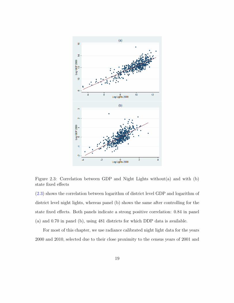
Figure 2.3: Correlation between GDP and Night Lights without(a) and with (b)state fixed effects
(2.3) shows the correlation between logarithm of district level GDP and logarithm of
district level night lights, whereas panel (b) shows the same after controlling for the
state fixed effects. Both panels indicate a strong positive correlation: 0.84 in panel
(a) and 0.70 in panel (b), using 481 districts for which DDP data is available.
For most of this chapter, we use radiance calibrated night light data for the years
2000 and 2010, selected due to their close proximity to the census years of 2001 and
19

2011. This ensures we have adequate data for additional district level controls. In a
subsection of this chapter, we also break up the study into two sub-periods of 2000-
2005 and 2005-2010 though for many demographic variables we need to interpolate
initial values for 2005. Over the ten year period, 47 new districts were created. While
there were 593 districts in 2001, by 2011 there were 640. To ensure consistency, we
summed up the data of the new districts to the district of origin if the new district
was created dividing a single district. If the new district was carved out from multiple
districts, we dropped both the new and the district of origin to avoid complications.
We also decided to drop the state of Assam as more than 50 percent of districts in
the state were redrawn. Our baseline regressions include 518 districts.
2.3.2 Empirical Methodology
To investigate the presence of absolute convergence, we estimate Equation (2.1):
gyi,t,t−k= βyi,t−k + εi,t,t−k (2.1)
where gyi,t,t−kis the average growth rate of night light per capita of district i between
years t(2010) and t−k(2000) and and yi,t−k is the logarithm of initial lights per person
in district i. ε is district specific random shocks. β in equation 1 represents the rate of
absolute convergence. A negative β suggests an inverse relationship between initial
condition and the growth rate implying convergence between the regions whereas
the magnitude of β measures the rate of convergence. We use the above equation
to look at aggregated, rural and urban convergence. Absolute convergence entails
that the growth rate of areas with poorer initial conditions will be higher. In other
20

words, inequality between districts will reduce even without any influence of other
factors. As is well known, this is not something that is observed in cross-country
data. On the other hand, at the cross country level ‘conditional convergence’ often
holds, implying that the growth rate of region converge to a long run (steady-state)
growth rate conditioned on variables that explain the long run values. Therefore, to
examine conditional convergence among districts, as well as rural and urban regions,
we estimate the following equation:
gyi,t,t−k= βyi,t−k + ηXi + fj + εi,t,t−k (2.2)
Where β gives us the rate of conditional convergence controlling for district char-
acteristics. ε is district specific random shocks similar to equation 1. Xi represents
district specific control variables for ith district, whereas η estimated the coefficient
of such controls. The Xi in our study includes initial district specific demographic
characteristics such as literacy rates, higher education attainment rates, scheduled
cast and scheduled tribe population shares, working population shares as well as
geographic variables such as population density and rainfall. It also includes infras-
tructure variables such as net irrigated land, connectivity to paved roads, access to
finance, and electricity connections. A negative β implies convergence in growth pat-
tern conditional on the district specific characteristics. and a higher magnitude of β
suggests a higher rate of conditional convergence. Finally, time invariant state char-
acteristics such as institutions, governance etc. might explain disparities in growth
rates of the districts. To take into account such variations, we also examine the
consequences of adding state fixed effects, fj, to both equations 2.1 and 2.2. We
21

discuss the sources and construction of the control variables further in Appendix A
at the end of this dissertation.
2.3.3 Data Summary and Correlation
Table (2.1) shows the summary of dependent and explanatory variables in our study.
The overall district sample uses 518 districts, whereas the total observations in rural
and urban areas are 506 and 474 respectively.2 The main variable of interest is the
‘Initial light’ defined as logarithm of per-capita light in the year of 2000 for growth
regressions of 2000-05 and 2000-10. Additionally 2005-10 growth regressions use log
per-capita night lights of 2005 as initial light. Both night lights growth and initial
lights are estimated for the overall district as well as rural and urban areas of the
districts separately.
The data for shares of population that belong to a scheduled caste (SC pop.
share), scheduled tribe (ST pop. share), are of working age (Working pop.share), are
literate (Literate pop. share), have higher education (Higher edu. share); fraction
of households that have electricity connections (Electricity connection), and credit
per capita (Log Credit p.c.) can be calculated for urban and rural areas separately.
Population density (Overall pop. Density) and rainfall per square kilometre (Log
Rainfall per sq km.) are for the entire district. For paved roads (Log HH with paved
roads), we use the whole district and also apply the same variable for rural areas
without further modification. In urban areas, roads are usually “paved” (even though
a significant portion might be abysmal by any objective standard). As a result even
though it is measured at the overall district level, it primarily reflects differences in
2514 out of 518 districts in our study has rural population and light data, but we have data forNet irrigated area for only 506.
22

23
Table 2.1: Data SummaryTotal Rural Urban
VARIABLES Observation Mean Observation Mean Observation MeanLights Growth p.c. (2000-10) 518 0.01 514 0.02 474 -0.01Lights Growth p.c. (2000-05) 518 -0.07 514 -0.09 474 -0.02Lights Growth p.c. (2005-10) 518 0.11 514 0.14 474 -0.01Log Initial Light p.c. (2000) 518 -4.28 514 -4.31 474 -4.17Log Initial Light p.c. (2005) 518 -4.61 514 -4.77 474 -4.23SC Pop. Share 518 0.15 514 0.17 474 0.13ST Pop. Share 518 0.15 514 0.17 474 0.05Working Pop. share 518 0.41 514 0.43 474 0.31Literate Pop. share 518 0.53 514 0.49 474 0.67Higher Edu. Share 518 0.07 514 0.04 474 0.16Electricity Connection 518 0.54 514 0.48 474 0.82Log Rainfall per sq km. 518 -3.72 514 -3.74 486 -3.761Log Credit p.c. 518 -4.27 514 -5.13 474 -3.04Rural Percent 518 0.78Overall Pop. Density 518 0.01 514 0.01 474 0.01Log HH with Paved Roads 518 4.00 514 4.00Log Net Irrigated Area 506 4.05
rural development. Similarly, net irrigated area (Log Net irrigated area) is used for
rural samples only. The share of rural population in total population (Rural Percent)
is only used in the overall district regression as an inverse measure of urbanization.
Apart from the expected differences in means between urban and rural areas of
districts, a highlight of this table is the average growth rates in lights per capita.
We can see that the average growth rate in urban areas was actually negative while
the average growth rate in rural areas was 2% points. This is not because of any
particular outlier. In the case of urban areas, exactly half experienced positive growth
in lights per capita while the remaining experienced negative growth. In the case of
rural areas, 348 of the 518 districts experienced positive growth while the remaining
170 experienced negative growth. Thus underlying our sample are very disparate
experiences when using light data.
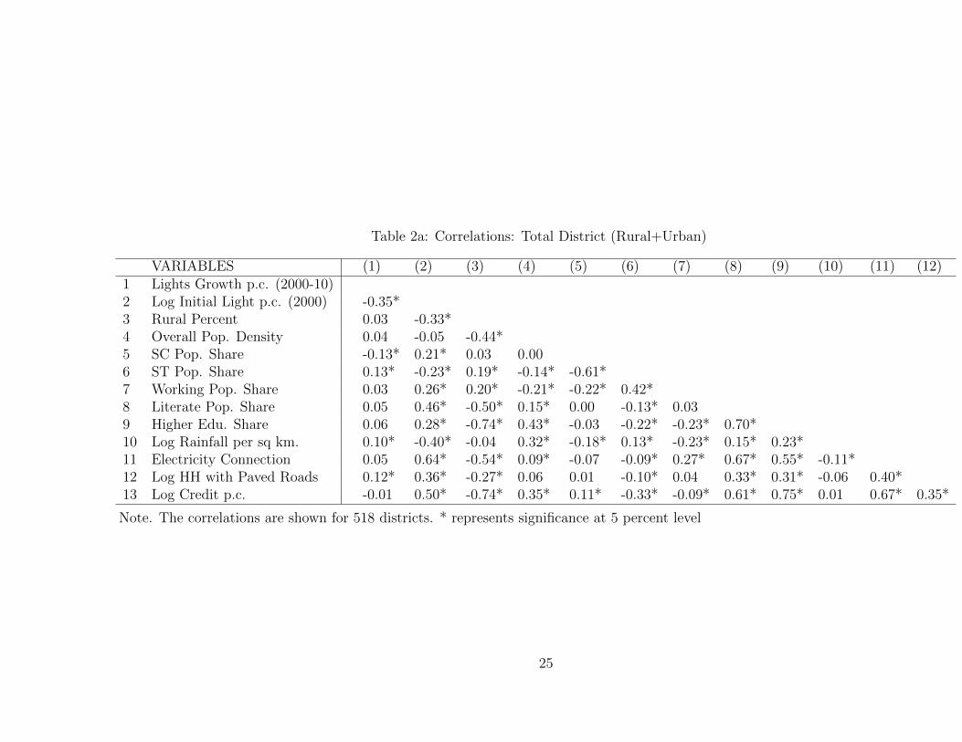
Tables 2a, 2b, and 2c show the correlations among dependent and independent
variables for total, rural and urban areas respectively. From Table 2a we can see
that the initial lights per capita has a negative correlation with growth in lights
per capita thus providing some prima facie evidence of absolute convergence. The
correlation between all of the control variables and growth in lights per capita is not
as compelling. We can also observe from column (2) that the initial lights per capita
is also negatively correlated with rural share of the population and rainfall while
it positively correlated with working age population share, literacy rates, higher
education attainment, electricity connection, roads and credit. Interestingly, the
relationship between lights per capita and the share of the population that belongs
to scheduled castes is positive while for scheduled tribes is negative. In other words,
24
25
Table 2a: Correlations: Total District (Rural+Urban)
VARIABLES (1) (2) (3) (4) (5) (6) (7) (8) (9) (10) (11) (12)1 Lights Growth p.c. (2000-10)2 Log Initial Light p.c. (2000) -0.35*3 Rural Percent 0.03 -0.33*4 Overall Pop. Density 0.04 -0.05 -0.44*5 SC Pop. Share -0.13* 0.21* 0.03 0.006 ST Pop. Share 0.13* -0.23* 0.19* -0.14* -0.61*7 Working Pop. Share 0.03 0.26* 0.20* -0.21* -0.22* 0.42*8 Literate Pop. Share 0.05 0.46* -0.50* 0.15* 0.00 -0.13* 0.039 Higher Edu. Share 0.06 0.28* -0.74* 0.43* -0.03 -0.22* -0.23* 0.70*10 Log Rainfall per sq km. 0.10* -0.40* -0.04 0.32* -0.18* 0.13* -0.23* 0.15* 0.23*11 Electricity Connection 0.05 0.64* -0.54* 0.09* -0.07 -0.09* 0.27* 0.67* 0.55* -0.11*12 Log HH with Paved Roads 0.12* 0.36* -0.27* 0.06 0.01 -0.10* 0.04 0.33* 0.31* -0.06 0.40*13 Log Credit p.c. -0.01 0.50* -0.74* 0.35* 0.11* -0.33* -0.09* 0.61* 0.75* 0.01 0.67* 0.35*
Note. The correlations are shown for 518 districts. * represents significance at 5 percent level

26
Table 2b: Correlations: Rural Areas
VARIABLES (1) (2) (3) (4) (5) (6) (7) (8) (9) (10) (11) (12)1 Rural lights growth p.c.2 Log Initial Rural Light p.c. -0.35*3 Overall Pop. Density -0.03 -0.31*4 Rural SC Pop. Share -0.13* 0.15* 0.25*5 Rural ST Pop. Share 0.12* -0.17* -0.40* -0.62*6 Rural Working Pop. Share -0.03 0.43* -0.60* -0.23* 0.37*7 Rural Literate Pop. Share 0.12* 0.41* -0.02 0.05 -0.14* 0.12*8 Rural Higher Education 0.17* 0.13* 0.17* -0.01 -0.19* -0.12* 0.69*9 Log Rainfall per sq km. 0.13* -0.43* 0.32* -0.16* 0.12* -0.30* 0.16* 0.28*10 Rural Electricity Connection 0.06 0.64* -0.24* -0.02 -0.08 0.41* 0.58* 0.36* -0.14*11 Log HH with Paved Roads 0.15* 0.35* -0.05 0.04 -0.10* 0.11* 0.31* 0.29* -0.08 0.38*12 Log Net Irrigated Area -0.35* 0.28* 0.25* 0.49* -0.51* -0.21* -0.12* -0.14* -0.48* 0.01 0.0413 Log Rural Credit p.c. 0.07 0.48* -0.10* 0.22* -0.20* 0.23* 0.37* 0.26* -0.13* 0.57* 0.32* 0.09
Note. The correlations are shown for 506 districts. * represents significance at 5 percent level

27
Table 2c: Correlations: Urban Areas
VARIABLES (1) (2) (3) (4) (5) (6) (7) (8) (9) (10)1. Urban Lights Growth p.c. (2000-10) 12. Log Initial Urban Light p.c. (2000) 0.1* 13. Overall Pop. Density 0.16* -0.04 14. Urban SC Pop. Share 0.16* 0.22* -0.04 15. Urban ST Pop. Share -0.13* -0.16* -0.09 -0.36* 16. Urban Working Pop. Share 0.09 0.19* 0.03 0.05 0.14* 17. Urban Literate Pop. Share 0.01 0.27* 0.04 -0.07 0.22* 0.44* 18. Urban Higher Edu. Share 0.07 0.06 0.03 -0.02 0.00 0.02 0.15* 19. Log Rainfall per sq km. 0.07 -0.31* 0.37* -0.19* 0.15* 0.06 0.20* 0.02 110. Urban Electricity Connection 0.02 0.53* 0.03 -0.01 0.08 0.40* 0.52* 0.08 -0.23* 111. Log Urban Credit p.c. 0.17* 0.33* 0.28* 0.01 -0.18* 0.28* 0.39* -0.06 0.12* 0.37*
Note. The correlations are shown for 474 districts. * represents significance at 5 percent level

the simple correlation seems to indicate that districts with larger scheduled caste
populations have already been faring better than those with large scheduled tribe
affiliations. This is not surprising since from Table (2.1), we can see that rural
areas tend to have larger scheduled tribe population shares while scheduled caste
population shares are more consistent across both urban and rural areas. If we look
at the percentage of the population that is rural in 2001, we can also see that it
is negatively correlated with many of the control variables such as literacy rates,
population density, higher education attainment, electricity connections, roads and
credit. In other words, the table reinforces some of the prior perceptions one might
have about the rural-urban dichotomy in India. Finally, the table also indicates that
roads, credit, and electricity are all correlated with each other and credit is also
correlated with education.
Similarly, Table 2b for rural areas shows negative correlation between the log of
initial lights per capita and growth in lights per capita. The infrastructure variables
are positively correlated with each other -showing that the rural areas in a district
with better electricity connection also have higher access to credit. Moreover, a
positive correlation can be observed between infrastructure variables and education
variables. In the case of Table 2c, contrary to the previous tables, a low but positive
correlation is depicted between initial urban lights per capita and subsequent growth
rates. Beyond that, the pattern of correlation in urban areas is similar to that of
their rural counterparts.
28

2.4 Results
2.4.1 Growth Regressions
In this section we present our basic empirical results for the overall districts as well
as rural and urban areas separately. Equations (2.1) & (2.2) are estimated taking
average growth in night lights per capita in the districts between 2000 and 2010 as
the dependent variable and initial lights per capita as the main variable of interest.
Additionally, we take into account the state fixed effects to control for state level
factors. Andhra Pradesh is the baseline state in our study. To mitigate the problem
of heteroskadasticity robust standard errors are used in all the regressions.
• Overall District Growth:
The regression results for the overall district for the period of 2000-10 is pre-
sented in Table (2.3). The first column shows the most parsimonious version of our
models, regressing the growth in lights per capita on the logarithm of initial lights
per capita. The β- coefficient is significant at 1 percent with a magnitude of -.018 and
the standard deviation is .004. This result indicates absolute convergence among the
districts. In the second column, we consider the effect of adding demographic vari-
ables. We include rural population shares, population density, shares of SC and ST
populations, and share of working population. The convergence coefficient remains
significantly negative with a higher magnitude (-.024) than in column (1). The coef-
ficient of the rural percentage is negative and significant at 1 percent level, whereas
the working population has a significant positive effect. population density, SC and
ST population share do not have significant impact on growth. Table 2a indicates
that initial lights per capita is correlated with a range of infrastructure and education
29

Table 2.3: District Growth, 2000-2010
VARIABLES (1) (2) (3) (4) (5) (6) (7)Dependent Variable: Overall Night Lights Growth per capitaLog Light p.c. (2000) -0.018*** -0.024*** -0.043*** -0.023*** -0.024*** -0.031***
(0.004) (0.005) (0.008) (0.006) (0.005) (0.006)Rural Percent -0.053*** 0.047** -0.037** 0.010
(0.015) (0.019) (0.016) (0.019)Overall Pop. Density -0.074 0.105 -0.058 0.139
(0.074) (0.109) (0.105) (0.101)SC Pop. Share -0.008 0.037 0.046 0.019
(0.026) (0.023) (0.040) (0.032)ST Pop. Share -0.009 0.012 0.022 0.023
(0.015) (0.015) (0.023) (0.019)Working Pop. Share 0.153** 0.056 -0.026 -0.000
(0.065) (0.049) (0.042) (0.040)Literate Pop. Share 0.071** 0.113***
(0.032) (0.035)Higher Edu. Share -0.017 -0.034
(0.109) (0.105)Log Rainfall per sq km. -0.009** -0.014***
(0.005) (0.004)Electricity Connection 0.070*** 0.043**
(0.018) (0.020)Log HH with Paved Roads 0.014*** 0.007***
(0.003) (0.003)Log Credit p.c. 0.007** 0.001
(0.003) (0.003)State Fixed Effect No No No Yes Yes Yes Yes
Constant -0.063*** -0.107*** -0.372*** 0.023*** -0.057*** -0.030 -0.278***(0.017) (0.040) (0.085) (0.002) (0.020) (0.029) (0.079)
Observations 518 518 518 518 518 518 518Adjusted R-squared 0.124 0.154 0.318 0.480 0.547 0.554 0.607
Note: The results presented here refer to the entire district, i.e. rural + urban.Robust standard errors are given in the parenthesis.∗∗∗ shows p− value < .01 , ∗∗ shows .01 < p− value < .05 and ∗ shows .05 < p− value < .1
30

variables in addition to demographic characteristics. In other words, even though
initial lights is negatively correlated with subsequent growth, it might be correlated
with other omitted variables that we have not controlled for. In the third column, we
incorporate the human capital accumulation and infrastructure variables along with
those used in column (2) to take into account such initial variations. We use initial
literacy rates and share of the population with higher education (completed higher
secondary or more) as indicators of human capital accumulation, whereas, infrastruc-
ture includes share of households with electricity connections and access to paved
roads, along with logarithm of credit per capita. Finally, we also include rainfall
to control for climate variation over the districts. In line with our expectations, all
the infrastructure variables have positive and significant effects on growth together
with share of literate population. Higher education is insignificant and so are other
demographic variables. Interestingly, the convergence coefficient increases to -.043
with inclusion of above controls indicating that many of these variables reflect long
run steady state conditions. The percentage of rural population in a district changes
signs from column (2) and becomes positively significant but as we shall see below
this is not robust. The coefficient of the logarithm of rainfall per square km. is neg-
atively significant. Finally, the addition of human capital, infrastructure and rainfall
doubles the adjusted R-square.
Since there is evidence that states have diverged during this time period, our
findings of convergence at the district level might be misleading if we do not account
for state fixed effects. From Column (4) onwards, we introduce state fixed effects.
Adding state fixed effects is also important since a large number of policies are
31

made at the state level. As a precursor, we run a regression of growth in lights
per capita on only state dummies in column (4) to show the extent to which the
state fixed effects explain growth in districts. The adjusted R-square depicts that
48% percent of district growth can be explained by state specific characteristics. In
other words, while districts have experienced very heterogenous growth rates, almost
half of the growth seems to be driven by variables at the state level. Column (5)
presents regression similar to column (1) with the state fixed effects. The convergence
coefficient remains significant at 1 percent with the magnitude of -.023. The Adjusted
R- square increases to 55% percent with inclusion of initial lights.
In column (6) & (7) we present the regressions similar to second and third column
including state fixed effects. The β- coefficient in column (6) is close to the same in
column (5). Similar to column (2), the percentage of rural population is negative and
significant. All other demographic variables remain insignificant. Column (7) shows
the broadest specification of our models where we include all the control variables
along with the state effects. The convergence coefficient is still negative and signifi-
cant with around 3 percent rate of convergence though it is lower than what we see
in column (3). In other words, even though states might be diverging, within states
there seems to have been a tendency towards convergence. Electricity connection,
paved road connections and share of literate population are consistently positive and
significant reflecting importance of infrastructure and human capital accumulation
for economic growth. The coefficient of credit per capita reduces considerably in size
and is insignificant in column (7). An interesting observation is that the coefficient
of the literate population share increases in magnitude (from .071 to .113), while
32

the coefficients of the infrastructure variables fall (electricity connection: .070 to
.043, paved road connection: .014 to .007, Credit: .007 to .001) with introduction of
the state effects. This result suggests that to some extent, state has a role to play
in building district level infrastructure, however human capital accumulation varies
even within states, and has influenced the growth of districts. Rainfall per square
km. affects growth negatively - similar to column (3). In a primarily rural country
like India, where agriculture mainly depends upon rainfall, this result is surprising
and may suggest that the growth in the past decade was mainly in non- agricultural
sector, where heavy rainfall might even be harmful for economic activity. Another
possibility is that excess rainfall might be bad for economic growth even in agricul-
ture. However, since we use logarithmic values, our results should not be sensitive to
this scenario. Moreover, in our study, we do not include Assam, one of the rainiest
states and with high agricultural production.
• Rural Growth:
As mentioned earlier, the rural-urban dualism is prominent in India from de-
mographic and socio-economic perspectives. Being a primarily rural country with
68 percent of the population residing in rural areas, rural growth has been a major
concern for economists in India. Since 1991, several policies as well as massive public
spending projects have been introduced to reduce disparity between rural and urban
areas. In light of this, we explore whether initially poorer rural areas have been
closing the gap with their richer counterparts.
In Table (2.4) we consider growth in rural night lights per capita as the depen-
dent variable to examine rural convergence (or divergence). In comparison to Table
33

Table 2.4: Rural Growth, 2000-2010VARIABLES (1) (2) (3) (4) (5)
Dependent Variable: Rural Night Lights Growth per capitaLog Initial Rural Light p.c. (2000) -0.019*** -0.044*** -0.026*** -0.033***
(0.004) (0.007) (0.006) (0.006)Overall Pop. Density -1.084 -0.369
(0.713) (0.636)Rural SC Pop. Share 0.023 0.014
(0.023) (0.031)Rural ST Pop. Share -0.005 0.017
(0.014) (0.016)Rural Working pop. Share -0.034 -0.054
(0.042) (0.037)Rural Literate Pop. Share 0.092*** 0.122***
(0.034) (0.036)Rural Higher Edu. share -0.024 -0.134
(0.158) (0.144)Log Rainfall per sq km. -0.018*** -0.017***
(0.005) (0.005)Rural Electricity Connection 0.053*** 0.040**
(0.013) (0.017)Log HH with Paved Roads 0.015*** 0.008***
(0.003) (0.003)Log Net Irrigated Area -0.012*** -0.005***
(0.002) (0.002)Log Rural Credit p.c. 0.011*** 0.005
(0.003) (0.003)State Fixed Effect No No Yes Yes Yes
Constant -0.065*** -0.246*** 0.030*** -0.059*** -0.203***(0.016) (0.067) (0.002) (0.019) (0.067)
Observations 506 506 506 506 506Adjusted R-squared 0.126 0.416 0.504 0.579 0.636
Note. Robust Standard errors are given in the parenthesis.∗∗∗ shows p− value < .01 , ∗∗ shows .01 < p− value < .05 and ∗ shows .05 < p− value < .1
34

(2.3), we exclude the rural population share from the set of demographic controls,
but include net irrigated area as a rural infrastructure variable in an otherwise com-
parable set of controls. The demographic and human capital controls along with
credit data are calculated for rural areas using values for rural areas provided by
the census along with rural populations. Population density, rainfall per sq km.,
paved road connection and net irrigated area are the only variables that we could
not distinguish for rural areas due to data limitations.
Similar to Table (2.3), column (1) of Table (2.4) reports the regression of rural
night lights growth per capita on logarithm of initial rural lights per capita. The
coefficient shows significant convergence in night lights with a rate of 1.9 percent.
Interestingly this is very close to the absolute convergence coefficient of for the entire
districts that we found in the earlier table. The adjusted R-square is at .125 depict-
ing that initial lights per capita alone explains 12.5 percent of growth in rural areas.
In column (2) we incorporate all district specific controls to estimate conditional
convergence in rural areas. Similar column (3) in the earlier table, the rural con-
vergence coefficient increases to -.044 - very close to that of overall district growth.
Population density has a negative and significant coefficient. Note that the popu-
lation density incorporates the rural and urban areas which may distort the sign of
the coefficient. The share of literate population and the infrastructure variables such
as electricity connection, paved road connection, and rural credit are significantly
positive consistent to our findings for overall districts. Surprisingly, even for rural
areas where agriculture is the primary occupation, rainfall per sq km along with net
irrigated area are negative and significant. It is quite possible that areas with higher
35

rainfalls continued to focus on farming while growth happened in more productive
rural non-farming occupations.
Column (3) presents the regression of the dependent variable only on state dum-
mies. Similar to the previous table, the state fixed effects solely explain more than 50
percent of the rural growth. In column (4), we run the regression similar to column
(1) but with state fixed effects. The rural convergence coefficient remains significant
at 1 percent level with a magnitude of -.026. Column (5) shows the regression results
with all our district levels controls along with the state fixed effects. The coefficient
for initial lights drops as they did for in the earlier table but is again very similar in
magnitude. Population density and rural credit per capita lose significance once we
introduce the state effects. However, the variables significant in column (2), such as
share of literate population, infrastructure variables other than credit, rainfall and
net irrigated area are still significant with the same signs. It is interesting to note
that similar to the overall district regressions, the coefficients of the infrastructure
variables reduce in magnitude once we introduce state fixed effect, however, at the
same time, the coefficient of the share of literate population increases. To summarize,
rural district growth patterns are very similar to that of the entire district. From
hindsight, some may view this as unsurprising given the extent of rural population
shares in India. However, given the rapid growth in India during this time period,
the strong correspondence might appear as surprising to others.
• Urban Growth:
The correlation between urbanization and per capita incomes remains one of
the strongest patterns in development at the country level Gollin et al. [2016]. The
36

strong relationship between urbanization and development is also observed at the
sub-national level Chanda and Ruan [2015]. Urbanization can take various patterns-
the growth of new towns or existing towns; or the continued expansion of large
cities that reinforce their advantages in a period of rapid growth. Here we do not
distinguish between these types of growth. For the regression analysis, we take the
same controls used in the rural growth regressions, but calculated for urban areas.3
Paved roads and net irrigated area have been excluded as since they largely capture
differences in rural areas.
We report the regression result taking urban night lights growth per capita as
the dependent variable in Table 2.5. Similar to the previous regression tables, we
report the absolute convergence coefficient in column (1). The coefficient is positive
and small (.003) but significant at 10 percent level, indicating absolute divergence
among the urban areas. Also, the adjusted R-square is very low (.006) indicating
that initial light explains very little of subsequent urban growth. Next, we include
urban controls along with overall population density and rainfall. The β-coefficient
still remains very small and becomes insignificant. Population density is positive and
significant implying a district with higher population per km shows higher growth in
light. Recall that population density is a district level variable. The variable likely
picks up the benefits to agglomeration in some districts. Some indication of this
comes from Table 2a - districts that have higher population densities also have lower
population shares. This is not surprising and certainly reflects some initial degree of
agglomeration. Finally, the share of the scheduled caste population in urban areas
3Similar to rural areas, population density and rainfall per sq km has not been distinguished forrural and urban areas. We use overall district data for these two variables.
37

Table 2.5: Urban Growth, 2000-2010
VARIABLES (1) (2) (3) (4) (5)
Dependent Variable: Urban Night Lights Growth per capitaLog Initial Urban Light p.c. (2000) 0.003* 0.002 0.003 0.002
(0.001) (0.002) (0.002) (0.002)Overall Pop. Density 0.154*** 0.125*
(0.057) (0.073)Urban SC Pop. Share 0.078** 0.046
(0.032) (0.029)Urban ST Pop. Share -0.006 0.019
(0.017) (0.031)Urban Working Pop. Share 0.052 0.063
(0.045) (0.054)Urban Literate Pop. Share -0.034 -0.002
(0.026) (0.031)Urban Higher Edu. share 0.014** 0.010**
(0.006) (0.004)Log Rainfall per sq km. 0.002 -0.000
(0.002) (0.002)Urban Electricity Connection -0.007 0.015
(0.017) (0.025)Log Urban Credit p.c. 0.005 0.006*
(0.003) (0.003)State Fixed Effect No No Yes Yes Yes
Constant 0.006 0.023 -0.004 0.007 -0.025(0.006) (0.024) (0.003) (0.009) (0.034)
Observations 474 474 474 474 474Adjusted R-squared 0.006 0.068 0.197 0.195 0.220
Note: Robust standard errors are given in the parenthesis. ∗∗∗ shows p− value < .01 ,∗∗ shows .01 < p− value < .05 and ∗ shows .05 < p− value < .1
has significant positive effect on urban growth. Unlike rural areas, the coefficient of
higher education in the urban area is positive and significant showing accumulation
38

of human capital in above secondary level has a role to play in urban growth. This
result is in contrast with the rural area where only literate population share has a
significant effect on growth. Thus while education is important for both areas, it is
clear that the thresholds are important. This is a useful result particularly given the
recurring ambiguity of the role of various education attainment measures in growth
regressions.
Column (3) presents the extent to which the the state dummies can explain urban
growth. The adjusted R-square is as low as 19.7 percent even with state dummies,
which rises to 22 percent once we include initial light and other controls in column
(5). In other words, unlike rural growth where states effects were more important,
urban areas seem to be less driven by state factors. In column (5) we present the
broadest model specification with all the controls and state effects. The coefficient
of initial light is still insignificant implying absence of conditional convergence. Only
population density and higher education along with urban credit are positively sig-
nificant at 10 percent level. The lack of significance of other infrastructure variable
and low R-square might indicate the presence of omitted variable problem. Accord-
ing to Das et al. [2015], convergence depends upon proximity to capital cities. Also,
urban regions might be growing because of the benefits they reap from other infras-
tructure projects such as access to the national highway system or perhaps access to
international trade. We plan to investigate the determinant of urban growth further
as future research, but at this stage what we see is that a range of initial conditions
are not useful in understanding patterns of urban growth.
39

2.4.2 Rural and Urban Spillovers
So far we have not discussed the issue of spillovers. There are two types of spillovers
– one is the standard theoretical notion of urban growth leading to in-migration and
as a result leading to not just urban growth but also raising the productivity of
adjoining rural areas as the marginal product of labor increases. Secondly, from an
econometric viewpoint, there might be an omitted variable problem of spillovers in
growth from adjoining areas. Here we consider the first kind of spillover. To see why
this might be important consider Figure 2.4.
Clearly, the logarithm of night lights per capita in the rural and urban areas
are positively correlated (using 477 observation the correlation is .57 without and
.36 with state effects).4 We examine the extent of rural urban spillovers in Table
2.6. As a straightforward exercise, we look at growth in rural, urban and overall
districts separately like before but control for initial light per capita from both rural
and urban areas in an effort to estimate the spillover effects on convergence. The
control variables (other than population density, rainfall, paved road connection and
irrigated area) in Table 2.6 represents total, rural and urban values in respective
regressions.
In first column of Table 2.6, we present regression using night lights growth
as dependent variable where main independent variables of interest are initial lights
(2000) per capita for both rural and urban areas. In line with our previous results, the
coefficient of initial rural light is negative and significant showing that the rural initial
condition affects district growth negatively. On the other hand, the initial urban light
4We use the districts with positive rural and urban lights. Delhi is an outlier with very low rurallights and high urban lights, hence dropped from the scatter diagram.
40

Figure 2.4: Relationship between Urban and Rural Night Lights in 2000, without(a) and with (b) state effects
does not affect district growth. The control variables behave similar to Table 2.3,
where literate population and paved road connections are still positively significant
whereas electricity connection and credit per capita lost significance. Column (2)
shows the similar regression for rural areas but also controlling for initial light of
urban areas in that district. Rural convergence is still present, though the rate of
convergence falls from 3.4 to 2.3 percent. Urban initial light does not affect rural
41

42
Table 2.6: Rural-Urban Spillovers
VARIABLES (1) (2) (3)
Dependent variable:
Total p.c.
Growth
(2000-10)
Rural p.c.
Growth
(2000-10)
Urban p.c.
Growth
(2000-010)
Log Initial Rural Light p.c. (2000) -0.021*** -0.023*** 0.008***
(0.004) (0.004) (0.003)
Log Initial Urban Light p.c. (2000) -0.002 -0.003 -0.001
(0.002) (0.002) (0.003)
Rural Percent -0.007
(0.017)
Overall Pop. Density -0.885 -0.456 1.826***
(0.595) (0.546) (0.463)
SC Pop. Share -0.017 -0.015 0.032
(0.027) (0.028) (0.032)
ST Pop. Share -0.014 -0.006 0.007
(0.014) (0.013) (0.054)
Working Pop. Share 0.005 -0.056 0.035
(0.036) (0.035) (0.058)
Literate Pop. Share 0.060** 0.067*** 0.022
(0.025) (0.025) (0.036)
Higher Edu. Share 0.012 -0.066 0.010**
(0.089) (0.113) (0.005)
continued on next page · · ·

43
VARIABLES (1) (2) (3)
Dependent variable:
Total p.c.
Growth
(2000-10)
Rural p.c.
Growth
(2000-10)
Urban p.c.
Growth
(2000-010)
Log Rainfall per sq. km. -0.005** -0.007*** -0.001
(0.002) (0.002) (0.002)
Electricity Connection 0.023 0.023* -0.011
(0.015) (0.013) (0.028)
Log HH with Paved Roads 0.007** 0.008**
(0.003) (0.003)
Log Credit p.c. 0.002 0.006** 0.002
(0.003) (0.003) (0.005)
Log Net Irrigated Area -0.003
(0.002)
State Fixed Effect Yes Yes Yes
Constant -0.144*** -0.098*** -0.005
(0.032) (0.034) (0.039)
Observations 478 474 470
Adjusted R-squared 0.572 0.585 0.191
Note: The independent variables in the rural and urban regressions takes the value rural and urban controlsrespectively. Only ‘Density’, ‘Rainfall’ and ‘Paved roads’ has not been classified between rural and urban
areas. Robust standard errors are given in the parenthesis.∗∗∗ shows p− value < .01 , ∗∗ shows .01 < p− value < .05 and ∗ shows .05 < p− value < .1

growth. The third column shows the urban growth regressions taking into account
the initial rural lights per capita of the district. Interestingly, the initial rural light
has a positive coefficient which is significant at the 1 percent level implying higher
growth in urban areas for districts where the rural areas were better off. In other
words, districts that were doing better in the rural areas also seem to have made a
successful transition into urban growth. As far as the remaining control variables are
concerned we continue to see a consistent pattern- of the asymmetric area-specific of
education and the role of population density in urban growth.
2.4.3 Examining Sub-Periods
The above sections show the evidence of convergence in rural areas that reflected in
convergence of overall district whereas not much can be inferred about the urban
growth. One might be interested in looking at the different sub-periods to explore if
the convergence among the districts or specifically, rural areas were consistent over
the decade. Also, several reform projects were implemented after 2005 which might
affect the growth pattern and thus change our result for the later half of the decade.
We divide the time period of our study to see if the convergence results as shown in
the last sections hold for both part of the decade. The growth rate night lights for
2000-05 and 2005-10 are used separately as dependent variables to run the regressions
similar to the last section. Table (2.7) shows the result of the regressions for rural
and urban areas along with the overall district. Column (1) & (2) shows the result
of growth regressions for overall districts whereas column (3) & (4), and (5) & (6)
show the same for rural and urban areas respectively. The independent variables,
though shown in the same table, take rural and urban values in rural and urban
44
regressions. Only population density, rainfall per sq km and paved road connections
have not been classified between urban and rural areas, thus take the same values in
all regressions. Due to data limitations, we control for the initial demographic, socio-
economic, and infrastructural conditions measured at the beginning of the decade
for both period regressions in our study.
The evidence of convergence is consistent in rural areas and overall districts
with our previous results. The magnitude of the rates of convergence are greater
in the second part of the decade in both cases showing that areas with lower night
lights in 2005 grew at around 5 percent faster than their counterparts. Interestingly,
the urban areas seem to diverge in the first half of the decade and converge in the
later half. However, for the second period the rate of convergence is far lower than
we we observe in rural areas. Given the diametrically opposite experiences with
urbanization in the two sub-periods, it is not surprising that the effect for the entire
ten year period is insignificant.
Among the control variables, rural percent has a positively significant coefficient
in 2005-10 regression, suggesting a rural bias in district level growth during the pe-
riod. Working population has negative effect on growth in the rural areas and overall
district during the first half and flips sign in the later half of the decade. In line with
our expectation, share of literate population has significant positive effect on rural
growth over both periods whereas initial population share with higher education in
urban areas affect urban growth favorably in the first part of the decade. This result
strengthens the case for increasing investment in education further. Infrastructure
variables such as connection to paved roads has positive and significant effect on
45
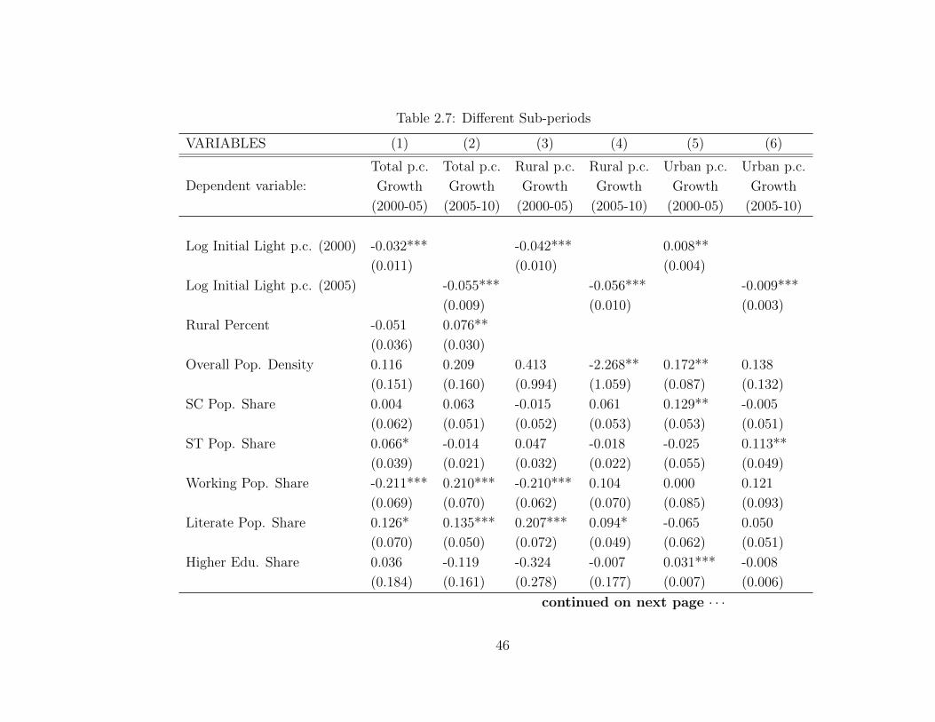
46
Table 2.7: Different Sub-periods
VARIABLES (1) (2) (3) (4) (5) (6)
Dependent variable:
Total p.c.
Growth
(2000-05)
Total p.c.
Growth
(2005-10)
Rural p.c.
Growth
(2000-05)
Rural p.c.
Growth
(2005-10)
Urban p.c.
Growth
(2000-05)
Urban p.c.
Growth
(2005-10)
Log Initial Light p.c. (2000) -0.032*** -0.042*** 0.008**
(0.011) (0.010) (0.004)
Log Initial Light p.c. (2005) -0.055*** -0.056*** -0.009***
(0.009) (0.010) (0.003)
Rural Percent -0.051 0.076**
(0.036) (0.030)
Overall Pop. Density 0.116 0.209 0.413 -2.268** 0.172** 0.138
(0.151) (0.160) (0.994) (1.059) (0.087) (0.132)
SC Pop. Share 0.004 0.063 -0.015 0.061 0.129** -0.005
(0.062) (0.051) (0.052) (0.053) (0.053) (0.051)
ST Pop. Share 0.066* -0.014 0.047 -0.018 -0.025 0.113**
(0.039) (0.021) (0.032) (0.022) (0.055) (0.049)
Working Pop. Share -0.211*** 0.210*** -0.210*** 0.104 0.000 0.121
(0.069) (0.070) (0.062) (0.070) (0.085) (0.093)
Literate Pop. Share 0.126* 0.135*** 0.207*** 0.094* -0.065 0.050
(0.070) (0.050) (0.072) (0.049) (0.062) (0.051)
Higher Edu. Share 0.036 -0.119 -0.324 -0.007 0.031*** -0.008
(0.184) (0.161) (0.278) (0.177) (0.007) (0.006)
continued on next page · · ·

47
VARIABLES (1) (2) (3) (4) (5) (6)
Dependent variable:
Total p.c.
Growth
(2000-05)
Total p.c.
Growth
(2005-10)
Rural p.c.
Growth
(2000-05)
Rural p.c.
Growth
(2005-10)
Urban p.c.
Growth
(2000-05)
Urban p.c.
Growth
(2005-10)
Log Rainfall per sq km. -0.022*** -0.013*** -0.027*** -0.014*** -0.002 -0.001
(0.008) (0.004) (0.009) (0.005) (0.003) (0.003)
Electricity Connection 0.060 0.076** 0.084** 0.043 0.101** -0.081**
(0.046) (0.036) (0.037) (0.032) (0.041) (0.041)
Log HH with Paved Roads 0.006 0.012*** 0.006 0.015***
(0.005) (0.004) (0.005) (0.005)
Log Net Irrigated Area -0.004 -0.006*
(0.004) (0.004)
Log Credit p.c. 0.009 -0.005 0.007 0.008 0.014*** 0.002
(0.007) (0.005) (0.006) (0.006) (0.005) (0.005)
State Fixed Effect Yes Yes Yes Yes Yes Yes
Constant -0.231 -0.522*** -0.329*** -0.277*** -0.004 -0.064
(0.153) (0.093) (0.127) (0.082) (0.060) (0.061)
Observations 518 518 506 506 474 474
Adjusted R-squared 0.497 0.505 0.524 0.415 0.386 0.153
Note: The independent variables in the rural and urban regressions takes the value rural and urban controlsregressions takes the value rural and urban controls respectively. Only ‘Density’, ‘Rainfall’ and ‘Paved roads’has not been classified between rural and urban areas. Robust standard errors are given in the parenthesis.
∗∗∗ shows p− value < .01 , ∗∗ shows .01 < p− value < .05 and ∗ shows .05 < p− value < .1

rural growth during 2005-10 whereas the share of households with electricity connec-
tion affects rural growth favorably during the first half. This result might reflect the
effect of public policy reforms taken during the period in the respective sectors. We
will discuss that in more details in next section of this chapter.
2.5 Public Projects and Rural Growth
While the previous sections presented evidence of rural convergence leading to the
overall district convergence, one might be concerned that rural growth during the
past decade may not reflect the standard neoclassical approach but the fruits of large
scale publicly financed projects implemented in Indian districts during this period.
Specifically, the growth in night lights may reflect the rapid increase in electricity
connections due to rural electrification project which was targetted at poorer dis-
tricts. Alternatively it might reflect economic growth due to the economic spillovers
from MGNREGS etc. To investigate further, we consider the effect of expenditures
on three large scale infrastructure and poverty reduction projects initiated by central
government during our study period. A large body of literature has already investi-
gated the association of rural poverty alleviation and district level growth with the
reform policies initiated during last two decades. Among them MGNREGS or rural
employment generation scheme has been popular in literature. Zimmerman (2012),
Imbart & Papp (2013), and Bhargava [2014] find significant effect of MGNREGS on
rural labor market, wages and adoption of agricultural technology. In similar vein, a
couple of recent papers by Aggarwal (2015), and Asher and Novosad [2016] examine
the effect of rural roads project (PMGSY) on agricultural advancement and sectoral
allocation of labor respectively. We consider the spending on rural employment gen-
48

eration project (MGNREGS), Rural road project (PMGSY) and a rural electricity
project (RGGVY) in our regression framework to examine if convergence still holds.
Unlike most of the existing literature, we measure the effectiveness of these projects
through incurred or sanctioned expenditures rather than physical outcomes. At best
our exercises are suggestive - there is no clear identification. However, our main pur-
pose here is to see if some of the convergence effects are driven by omitted variables.
We should also note that these are certainly not exhaustive. Most importantly we
do not have sufficient data on a number of education and health projects as well
as some rural credit expansion schemes. However since most of the education and
health projects are targeted to school age children, it is not clear that they would
have had a significant short-term impact on growth anyways. We briefly describe
the projects below before discussing the results.
• MGNREGS (Rural Employment Generation Project):
We begin with Mahatma Gandhi National Rural Employment Guarantee Scheme
based on Mahatma Gandhi National Rural Employment Guarantee Act (NREGA
2005) which is one of the largest public development schemes in the world. Envisioned
to secure the livelihood of the households in the rural areas of India, MGNREGS was
chartered as means to provide a legal guarantee of 100 days of public-sector wage em-
ployment in every fiscal year for adult members of the household who volunteered to
enroll for unskilled manual labor. It was implemented in three phases which started
with phase one implementation of 200 most backward districts in 2006. 130 more
districts were incorporated in phase two in 2007. In 2008, phase three of the pro-
gram included all remaining rural districts in the country. While it was initiated to
49

reduce rural poverty and involved employing rural workers in public projects during
low season for agriculture, it could have the potential effect of crowding out private
investment by raising wages. Thus the growth effects may be ambiguous. As our
control variable, we take the disbursed labor and material expenditure data for each
districts from the Ministry of Rural Development (MoRD). There has been consider-
able controversy about administrative waste in the program. Thus, if any effects show
up in our regressions, it would be an overestimate of the effect of the program.5 The
public data portal of MGNREGA shows physical and monetary variables reported
by the districts to MoRD. We use the data from 2006, the year of introduction of
the program, till 2010. The variable is constructed as total expenditure in a district
per unit of rural population.
• PMGSY (Rural Road Project):
Pradhan Mantri Gram Sadak Yojana (PMGSY) was launched in December 2000
to provide connectivity by construction of all weather road (operable throughout
the year) in the eligible unconnected habitations in rural India. The priority and
eligibility for inclusion of the unconnected habitation under the program were based
on population of the area. All unconnected habitations with a population of 1000
persons and above were planned to be covered in first three years (2000-2003), while
all unconnected habitations with a population of 500 persons and above were to be
covered by the end of the Tenth Plan Period (2007).6 The data for PMGSY has
been obtained from Online Management, Monitoring and Accounting System (OM-
5We could not include administrative expenses due to inconsistencies in the website.6 Any habitation in the Hill States (North-East, Sikkim, Himachal Pradesh, Jammu and Kash-
mir, Uttaranchal), the Desert Areas (identified in the Desert Development Programme), and thetribal areas would be eligible to be covered if the population of the area was 250 persons and above.
50

MAS) website where the district level summary of annual sanctioned expenditure
is provided from 2000 to present. We take the data relevant to our study period
(2000-2010). The control variable construction is given in the Data Appendix A.
• RGGVY (Rural Electrification Project):
Rajiv Gandhi Grameen Vidyut Yojana (RGGVY) was initiated in 2005 with
three objectives, firstly, to electrify all unelectrified villages and habitations and
intensify the process in already electrified villages; secondly, to equip all rural house-
holds with electricity connection; and thirdly, to provide free electricity connections
to all below poverty line households. The Rural Electrification Corporation Limited
was appointed by Ministry of Power of the Indian government to serve as the nodal
agency to implement the scheme. RGGVY was started in 2005 with a mandate to
attain the National Common Minimum Programme (NCMP) goal of providing elec-
tricity to all households by 2010, which then extended to 2012 in 11th five year plan.
However, due to slow implementation pace, the program had been extended in the
12th five year plan (2012-17) where it has been subsumed in Deen Dayal Upadhyay
Gram Jyoti Yojana (DDUGJY) as the rural electrification component of the pro-
gram. RGGVY data is obtained from the Ministry of Power website provided by
Government of India. The description of the variable used is given in Appendix A.
2.5.1 Results
A summary of total expenditures in these projects per unit of rural population is
presented in Table 2.8. The unit of the expenditure per capita is expressed in rupees.
The table shows that total disbursed labor and material cost of NREGA per unit of
rural population is around Rs. 1474.16 whereas the annual sanctioned expenditure
51

Table 2.8: Rural Public Projects: Expenditures per capita (in Rs.)
Variable Obs Mean DurationYears usedin this study
NREGA (Labor and material cost) 506 1474.16 2005 - present 2005-2010PMGSY (Road expenditure) 506 1704.45 2000 - present 2000-2010RGGVY (Sanctioned electricityexpenditure)
506 708.90 2005 - 2012 2005-2010
Table 2.9: Correlations: Public Project Expenditures per capitaVariable Obs (1) (2)Log Total Expenditure in PMGSY per capita 506Log Total Expenditure in NREGA per capita 506 0.33*Log Total Expenditure in RGGVY per capita 506 0.68* 0.37*
per capita of PMGSY Rs. 1704.45. Unlike the other two projects, we used plan-wise
data for RGGVY where most of the districts received grant only once during our
study period. The total expenditure per unit of rural population during our study
period is around Rs. 708.90. It is important to note that both NREGA and RGGVY
have been started at the second half of the decade and the data we use is for the
period of 2005-06 to 2010, whereas the data for the PMGSY data is for 2000-2010.
The correlations between the logarithm of project expenditure per capita are
presented in Table 2.9. We find significant correlations between all three project
expenditures. The infrastructure projects, road and electricity expenditure have a
correlation as high as .68 whereas the correlation coefficient of such projects with
NREGA are .33 and .37 respectively. The correlations are in line with our expecta-
tion, as all of the project were implemented by prioritizing poorer districts.
In Table 2.10, we show the regression results for the rural areas with the same
specification as column (5) of Table 2.4 but now controlling for the expenditure on
52

53
Table 2.10: Growth Effects of Rural Public Projects
VARIABLES (1) (2) (3) (4)
Dependent variable: Rural Night Lights Growth per capita
Log Initial Rural Light (2000) p.c. -0.033*** -0.032*** -0.035*** -0.033***
(0.006) (0.006) (0.007) (0.006)
Log PMGSY Exp. p.c. 0.002
(0.004)
Log NREGA Exp. p.c. -0.004**
(0.001)
Log RGGVY Exp. p.c. 0.001
(0.003)
Log Combined Exp. p.c. -0.004
(0.004)
Overall Pop. Density -0.318 -0.469 0.215 -0.503
(0.657) (0.621) (0.904) (0.641)
Rural SC Pop. Share 0.015 0.028 -0.006 0.019
(0.031) (0.031) (0.038) (0.030)
Rural ST Pop. Share 0.015 0.024 0.019 0.021
(0.017) (0.017) (0.020) (0.017)
Rural Working Pop. Share -0.057 -0.051 -0.045 -0.050
(0.038) (0.037) (0.043) (0.038)
Rural Literate Pop. Share 0.122*** 0.113*** 0.134*** 0.122***
(0.036) (0.036) (0.042) (0.036)
continued on next page · · ·

54
VARIABLES (1) (2) (3) (4)
Dependent variable: Rural Night Lights Growth per capita
Rural Higher Edu. share -0.124 -0.124 -0.154 -0.133
(0.143) (0.144) (0.198) (0.147)
Log Rainfall per sq km -0.017*** -0.017*** -0.020*** -0.017***
(0.005) (0.005) (0.005) (0.005)
Rural Electricity Connection 0.043** 0.034** 0.051** 0.039**
(0.018) (0.017) (0.023) (0.018)
Log HH with Paved Roads 0.008*** 0.008*** 0.009** 0.008***
(0.003) (0.003) (0.003) (0.003)
Log Net Irrigated Area -0.005** -0.006*** -0.007*** -0.006***
(0.002) (0.002) (0.003) (0.002)
Log Rural Credit p.c. 0.005 0.004 0.009** 0.005
(0.003) (0.003) (0.004) (0.003)
State Fixed Effect Yes Yes Yes Yes
Constant -0.194*** -0.215*** -0.208*** -0.216***
(0.069) (0.067) (0.069) (0.067)
Observations 500 504 413 506
Adjusted R-squared 0.635 0.638 0.620 0.635
Note: The unit of project investment given in Rs. Lakh. Robust standard errors are given in the parenthesis.∗∗∗ shows p− value < .01 , ∗∗ shows .01 < p− value < .05 and ∗ shows .05 < p− value < .1

reform projects. In column (1), (2) & (3) we include logarithm of total expenditure
per capita in the rural road project (PMGSY), rural employment project (NREGA)
and rural electricity project (RGGVY) respectively. There are no significant effects
of infrastructure development projects such as PMGSY and RGGVY on rural night
lights growth. The coefficient of expenditure on NREGA is perversely, negative and
significant at the 10 percent level. The convergence coefficient remains at around
3.3 percent, close to our basic regression results in the rural areas. Similarly, initial
human capital and infrastructure such as literate population, household share with
paved road connection, rural electricity connection have significantly positive coeffi-
cients. Rainfall per square km. and net irrigated area on the other hand negatively
affect rural growth as before. Rural credit per capita is only significant in column
(3) when we include the electricity expenditure only.
As the correlation between the project expenditures is significant, it is possible
that the total expenditure on all three projects combined may have influenced rural
growth in a district even when the individual project expenditures does not have
any significant impact on the same. We present rural regression with the sum of the
project expenditures per capita in column (4). The coefficient of the sum of project
expenditure is still insignificant and there is very little change in the convergence
coefficient and other control variables. These results emphasize our claim that the
initial conditions has a major role in explaining rural growth, thus strengthening the
case of rural convergence. Nonetheless a more careful treatment of identification is
warranted before we can reach any firm conclusion about these projects.
55
2.6 Conclusion
Our analysis of the pattern and determinants of local growth using 518 districts in
India enables certain findings. First, we find evidence of both absolute and condi-
tional convergence in the overall districts primarily driven by rural convergence. The
convergence rate stands at around 3%, greater than Barro’s “iron law”. There is no
evidence of convergence in the urban area. Second, the initial measure of human
capital along with Access to road, credit and electricity connection are strongly as-
sociated with both urban and rural growth. In the case of human capital literacy
rate plays a role in defining the rural growth whereas, higher education is related
to urban growth. Moreover, State effects explain almost half of the district level
growth. However, the range of initial conditions used in our study explain very little
of urban growth. Finally, we fail to find any significant evidence to associate three
major rural reform projects with rural growth. Although a more careful treatment of
identification are necessary to draw any conclusion about these projects, this result
strengthens our case of rural convergence.
We conclude with certain limitations that can lead to future research. This
chapter uses data for 2000, 2005 and 2010 to measure long run growth where it may
be useful to collect the data for consecutive years to calculate annual growth rate.
Furthermore, our analysis explains very little of urban growth pattern. An obvious
step forward is to gather more informations on urban areas, for example, proximity to
capital cities, urban infrastructure projects, to recognize the determinants of urban
growth. Finally, it may be helpful to do a spatial analysis on the district growth
pattern to determine if the growth of a district is affected by its neighbours.
56
Chapter 3Effect of Credit Supply Shock onGrowth
3.1 Introduction
The importance of bank credit as a share of GDP has increased steadily over last
couple of decades in India. Additionally, several government initiatives have been
taken to increase credit generation and other financial services. For example, the
Prime Minister Jan Dhan Yojana, a financial inclusion project, prompted 180 million
new accounts within a year of its launching in 2014. There is evidence in the literature
that negative credit shocks affects economic activity (Bernanke and Blinder [1992],
Chodorow-Reich [2014], Iyer et al. [2014]). However, the magnitude and mechanism
of such impact is less understood ([Paravisini et al., 2015]). In this chapter, we
investigate the effect of bank credit shock on regional economic growth using district-
level outstanding credit data of 511 districts in India from 2000-2010.
We find evidence of positive and significant association between per capita credit
growth and the per capita growth in economic activity over our study period. How-
ever, it is hard to distinguish between the supply side growth in credit and demand
driven credit shocks. To disentangle these effects, we use the shift share instrument to
estimate predicted growth controlling for the district specific demand shock in credit.
For identification, we exploit the heterogeneity of initial sectoral share of outstand-
ing credit, which is originated by the scheduled commercial banks. While there is a
significant and positive relationship between the predicted shock in the credit supply
57

and the overall credit growth in the district, the predicted credit supply shock fails
to affect economic growth.
3.2 Background
To provide some context, we first look at the national trends in credit origination in
India over the past two decades. Figure 3.1 shows the trend in overall credit-to-GDP
ratio from 1996 to 2012.
Figure 3.1: National trend in credit to GDP ratio
Starting at around 20%, there has been a steady rise in the ratio over most of the
period. There was a slight decline in 2010, but subsequently experienced increase in
credit as a percent of GDP upto 53.5%. This steady upward trajectory implies that
credit growth has outpaced economic growth during this time period.
Taking one step further, we explore the growth in national credit in different
sectors over the period of our study. The trend in real sectoral credit is presented in
Figure 3.2.
58

Figure 3.2: National trend in real sectoral credit relative to Agriculture
Figure 3.3: National trend in real sectoral credit to GDP ratio
There has been a substantial growth in professional service sector, personal loans,
and financial sector credit. Credit in trade, industry, and unspecified other credits
grew at a much lower rate. A more comprehensive understanding about the sectoral
59

Table 3.1: Sectoral Growth in GDP & Credit (2000-2010)Growth rate of GDP Growth rate of Credit
Agriculture 0.03 0.15Industry 0.08 0.14Trade 0.09 0.09Finance 0.10 0.21Transport 0.08 0.21
credit is presented in Figure 3.3. We could match the sectoral credit with sectoral
GDP for agriculture, trade, transport, industry, and finance. The line showing credit-
to-GDP ratio in industries (for example, mining and manufacturing), lies well above
the same for all other sectors, and additionally, it is growing at a steady rate from
2004 onwards. For the other three sectors (i.e., agriculture, finance, and transport),
the ratio has increased slightly. Table 3.1 shows the national growth in sectoral GDP
and sectoral credit for the matched sectors.
The national trend in overall and sectoral credit depicts an ever growing depen-
dence on credit. Greenstone et al. [2014] has explored the impact of credit supply
shock on overall and small business employment over 1997-2011. Using a modified
shift share approach, they showed that the predicted lending shocks are associated
with significant but small decline in both country level and small business employ-
ment during the Great Recession. However, they fail to find any evidence of the
credit supply shock on employment in “normal times”. Amiti and Weinstein [2013]
has shown a substantial impact of credit supply shock on the investment decisions
of the firm. Paravisini et al. [2015] established that in trade, credit supply shock
has a significant impact on the intensive margin of export but does not affect the
extensive margin. In close association, we explore the impact of credit supply shock
60

on economic growth in Indian districts. As mentioned in the previous chapter of this
dissertation, the main concern in measuring regional growth in economic activity in
a developing country like India, is the lack of sub-national GDP data. Even when
present, the measurement quality of the data is questionable at best. We use radi-
ance calibrated satellite night light data to measure the growth in economic activity
similar to the previous chapter.
The rest of the chapter is organized as follows. Section 3.3 provides the data
sources, and Section 3.4 explains the empirical methodology. In Section 3.5, we
discuss our regression results. Finally, we conclude in Section 3.6.
3.3 Data
3.3.1 Night Light Data
We use radiance calibrated light data (used in the previous chapter) collected from
NOAA’s National Geophysical Data Center (NGDC) for the years 2000 and 2010.
3.3.2 Credit Data
The main variable of interest is district level credit for the years 2000 and 2010. We
use the data collected from ‘Basic Statistical Returns’ published by the Reserve Bank
of India . The data consists of the outstanding credit originated by the scheduled
commercial banks to various sectors of the economy. The main credit sectors in our
data are defined as agriculture, industry, transportation, personal, professional and
other services, trade, finance, and all other credits. We summed up the sectoral
credit to find overall credit in each district. Figure 3.4 shows the average share of
the sectoral credit relative to the total credit in the districts for 2000 and 2010. It
is evident that agriculture (27%) and industry (25%) captures the lion’s share of
61

Figure 3.4: Distribution of credit among main sectors in 2000 & 2010
the credit originated by the scheduled commercial banks in 2000, whereas service
and finance sector credit share are among the lowest. The share of agriculture tends
to increase even higher to 33%, while the share of industrial credit falls to 17 % in
2010. Among others, there has been an increase in the share of personal loan (17
% to 27%) and service sector credit (3% to 5 %). At the same time, the share of
credit in trade, transport, and other unspecified sector has declined over the decade.
Figure 3.5 presents the real growth rate among the sectoral credit (for the districts in
this chapter) more extensively. It is interesting to note that the average growth rate
is highest for the two sectors with lowest initial share, namely, finance and service.
Growth in personal loan and agriculture is also substantial in line with the findings
from Figure 3.4.
Next, we calculate the yearly growth rate of total credit over 2000 and 2010. As
the nominal credit data collected from RBI is not comparable between the years, we
62

Figure 3.5: Average growth rate of sectoral credit (2000-2010)
estimate the real credit at 2004-05 price, using state level GDP deflators, calculated
from the state GDP data, published by RBI. Figure 3.6 shows the kernel density of
log total credit in 2000 and 2010. There is a pronounce rightward shift in the density
functions from 2000 to 2010.
Our primary focus in this chapter is to explore the relationship between credit
growth and the growth in economic activity. We find positive correlation of .28
among the variables, whereas the correlation goes down to .13 if we control for the
state characteristics. Figure 3.7 show the scatter plot of the relationship with (Panel
B) and without (Panel A) controlling for state dummies.
For the rest of this chapter, we use credit and radiance calibrated night light data
for 2000 and 2010. As in the previous chapter, these years were selected to ensure that
we have adequate data for additional district level controls taken from the census
of 2001 and 2011. Table 3.2 shows the summary of the dependent, independent
63

Figure 3.6: Kernel Density of log Total Credit for 2000 and 2010
and control variables. As mentioned earlier, we summed up the data from the new
district created during this 10 year period with the district of origin, to maintain
consistency, if the district of origin is singular. If the new district was carved out
from multiple districts, we dropped both the new and the district of origin. We
also drop the state of Assam as more than 50 percent of districts in the state were
redrawn. Moreover, the credit data is available for 560 districts out of 593 in 2000,
whereas credit data for 631 districts is available for the year 2010. After eliminating
the missing observations, our baseline regressions include data from 511 districts.
The main variable of interest is the ‘Per capita credit growth’ between 2000 and
2010, defined as the average annual log change in total credit net of log change in
population . Similarly, the dependent variable ‘Per capita light growth’ measure
the log change in light net of log change in population per year. We use data for
shares of population that belong to a scheduled caste (SC pop. share), scheduled
64

Figure 3.7: Correlation between per capita credit growth and per capita light growth(A) without and (B) With controlling state dummies
tribe (ST pop. share), are of working age (Working pop.share), are literate (Literate
pop. share), have higher education (Higher edu. share); fraction of households
that have electricity connections (Electricity connection) collected from census 2001.
Rainfall per square kilometre (Log Rainfall/sq km.) is collected from the University
65

Table 3.2: Summary StatisticsVariable Obs Mean Std. Dev.Per capita light growth 511 0.01 0.04Per capita credit growth 511 0.12 0.05Log initial light per capita 511 -4.28 1.00Log area (sq me) 511 22.02 0.86Share of SC pop. 511 0.15 0.08Share of ST pop. 511 0.15 0.25Share of working pop. 511 0.41 0.07Share of literate pop. 511 0.53 0.12Share of higher educated 511 0.07 0.04Log rain/sqkm 511 -3.66 1.15HH with electricity 511 0.55 0.27
of Delaware website. We can see that the average growth rate in light per capita 1.1
percent, whereas the average per capita growth rate in credit remains at around 12
percent. It is interesting to note that 338 out of 511 districts in our study experience
positive light growth whereas 507 districts experience positive credit growth.
3.4 Empirical Design
Our empirical design is based on the observation that the credit growth rate among
the sectors varies substantially. Table 3.3 shows the variation in sectoral credit
growth. While the growth in financial and service sector credit are as high as 21.3%
and 18.7% respectively, growth in trade and industry credit are around 9%.
Furthermore, we exploit the heterogeneity in proclivity of each sector in the dis-
tricts, measured by initial credit share, for our identification strategy. We assume
that the borrowers of a certain sector cannot easily relocate to another sector depend-
ing upon the credit supply in that sector. Table 3.4 shows the summary statistics of
the sectoral credit share among the districts. It is evident that the standard deviation
66

Table 3.3: Credit Growth in SectorsSectors Growth rate of sectoral creditAgricuture 12.99Finance 21.33Industry 8.70All other 1.17Personal 16.73Service 18.91Trade 9.03Transport 7.05Total 13.29
Table 3.4: Sectoral credit share2000 2010
Sectors Obs Mean SD Mean SDAgricuture 511 0.27 0.15 0.33 0.19Finance 511 0.01 0.02 0.01 0.02Industry 511 0.25 0.17 0.19 0.16All Other 511 0.08 0.06 0.03 0.03Personal 511 0.17 0.07 0.27 0.14Service 511 0.03 0.03 0.05 0.05Trade 511 0.16 0.07 0.11 0.06Transport 511 0.03 0.03 0.02 0.02
among the agricultural and industry shares are the highest, whereas the variation in
the share are lower for the finance, service and transport sectors.
Next, we investigate the relationship between per capita growth rate of credit
and night light using the following primary equation.
gi,t,t−kntl = βgi,t,t−k
credit + γXi + εi,t,t−k (3.1)
Where gi,t,t−kntl is the average growth rate of night light per capita and gi,t,t−k
credit
is the growth rate of credit in district i between years t(2010) and t − k(2000). Xi
67

represents district specific control variables for ith district, whereas γ estimates the
coefficient of such controls. ε is district specific random shocks. β is the main
parameter of interest representing the relationship between credit growth and night
light growth. However, estimation of equation (3.1) is unlikely to produce unbiased
estimation of β because, the unobserved district characteristics may affect the growth
in economic activity and also be correlated with the credit growth. Moreover, the
credit growth can be viewed as the equilibrium of increase in demand and supply
in the credit market. It is difficult to distinguish the supply shocks apart from the
demand shocks. To overcome such identification issues and separate out the credit
supply effect, we build a shift share instrument following Greenstone et al. [2014].
First, we estimate equation (3.2)
gij,t,t−kcredit = di + sj + eij (3.2)
where the gij,t,t−k is the credit growth rate in district i and sector j. We use the initial
share of credit in district i and sector j (csij), to weight the equation. di in equation
(3.2) is the district specific dummies to control for the demand shocks in the districts
during our study period. The main parameters of interests are the coefficients (sj)
of the sector specific dummies sj. sj represents the weighted credit growth rate that
can be attributed to sector j relative to the reference sector, in our case, agriculture.
We estimate (sj) for each sector and re center the weighted coefficients to it’s mean.
Once we have the sector specific supply shock in credit, we replace the sectoral
credit growth rate in equation 3.2 by the same. The new modified shift share in-
strument ZSi , which represents the predicted credit supply shock in the economy, is
68

defined by the following equation:
ZSi =
∑j
(csij × sj) (3.3)
The methodology of modified shift share instrument, presented in 3.3, to purge the
demand shock has been used in literature. Khwaja and Mian [2008] has used such
instrument to separate out firm specific demand shock for bank-firm lending data
in Pakistan. Amiti and Weinstein [2013] has used the same methodology for the
Japanese data to investigate the supply side effect of financial shock on firm level
investment.
The exclusion restriction for the validity of the instrument can be written as :
Cov(ZSi εi,t,t−k) = 0 (3.4)
Intuitively, the identifying assumption is now weaker than the previous case. It
requires that the sectors with below average supply shock are not systematically dis-
tributed in the districts with below average credit shock. To validate our assumption,
we calculate the correlation between the coefficient of district fixed effects and the
initial credit share weighted sector fixed effect from equation 3.2. We find no cor-
relation between the fixed effects, thus validating our assumption that the districts
with low credit growth are not systematically exposed to the sectors with low supply
shock.
69

3.5 Results
In this section we present our basic empirical results using ordinary least square and
IV regression methods. We estimate equation 3.1 with and without the instrument
specified in the previous section. Additionally, we use state dummies to control for
state level factors. Andhra Pradesh is the baseline state in our study. Moreover, to
mitigate the problem of heteroskadasticity, robust standard errors are used in all the
regressions.
3.5.1 Ordinary Least Square
First, we present the ordinary least square regression estimation in Table 3.5. The
first column shows the most parsimonious model regressing per capita light growth
on growth in credit per capita. The coefficient is significant at 1% level showing that
a percent increase in credit growth is associated with .25 percentage point growth
in light with a standard deviation of .040. Column (2) includes socio-demographic
factors along with rainfall and electricity connection. The coefficient of credit growth
is significant and a little lower (.24) than the first column. Initial light is negatively
significant demonstrating convergence among the districts consistent with the first
chapter of this dissertation. Additionally, electricity connection is positive and sig-
nificant showing that a high initial electricity connection in a district is positively
associated with per capita light growth. Next, we regress the variable of interest
along with only state dummies to explore the extent of light growth per capita has
been explained by state characteristics. The credit growth coefficient falls to .091
but remain significant at 1%. The adjusted R2 jumps up to .49 from .085 (in column
1) as we include the state dummies. The fourth column of Table 3.5 presents the
70

Table 3.5: OLS Regression
(1) (2) (3) (4)
VARIABLESLight
growthper capita
Lightgrowth
per capita
Lightgrowth
per capita
Lightgrowth
per capita
Credit growth per capita 0.254*** 0.244*** 0.091*** 0.097***(0.040) (0.039) (0.035) (0.032)
Log per capita initial light -0.025*** -0.019***(0.003) (0.003)
Log area 0.004 0.004(0.004) (0.004)
SC pop. share 0.030 -0.001(0.020) (0.028)
ST pop. share -0.007 -0.008(0.011) (0.012)
Working pop. share 0.006 -0.031(0.033) (0.037)
Literate pop. share 0.033 0.063***(0.025) (0.024)
Share of higher educated 0.050 -0.005(0.064) (0.062)
Log rain/sqkm -0.001 -0.003(0.003) (0.003)
Electricity connection 0.045*** 0.028*(0.011) (0.014)
State dummies No No Yes Yes
Constant -0.018*** -0.255*** 0.049*** -0.177**(0.005) (0.082) (0.005) (0.089)
Observation 511 511 511 511Adjusted R2 0.085 0.234 0.497 0.558
Robust standard errors are given in the parenthesis.∗∗∗ shows p − value < .01 , ∗∗ shows .01 < p − value < .05 and ∗ shows.05 < p− value < .1
71

broadest model specification including both district characteristics and state dum-
mies. The coefficient of credit growth remains significant with a magnitude of .097
and a standard deviation .03. Initial light and electricity connection continues to
show the same sign as column (2) although the magnitude of the coefficient drops
with introduction of state dummies. Share of literate population becomes significant
at 1% level in column (4).
3.5.2 First Stage Regressions
Next, we calculate predicted credit growth rate from equation 3.3 and present the
relationship of such predicted growth and the actual credit growth in the districts.
Table 3.6 shows the first stage regressions. The first column presents the uni-variate
regression of original credit growth on the predicted credit growth. The coefficient
with a magnitude of .74 shows strong positive association significant at 1% level.
The second column includes the district characteristics whereas column (3) & (4)
repeats the regression on column (1) & (2) respectively along with state dummies.
The positive and significant relationship between predicted and original credit growth
persists all through the models. The fourth column shows the highest magnitude of
the coefficient at .949.
Having established a significant positive relationship between the instrument and
the variable of interest, we turn to the first stage statistics for the validity of our
instrument. Table 3.7 shows the 1st stage statistics from an uni variate regression
when the endogeneous regressor credit growth per capita is instrumented by per
capita predicted growth. Kleibergen-Paap F statistics is at 20.34 above the critical
rule of thumb value of 10 validating our instrument. Cragg-Donald F statistics for
72

Table 3.6: First Stage Regression
(1) (2) (3) (4)
VARIABLESCreditgrowth
per capita
Creditgrowth
per capita
Creditgrowth
per capita
Creditgrowth
per capita
Zi 0.744*** 0.928*** 0.660*** 0.949***(0.165) (0.195) (0.181) (0.215)
Log per capita initial light -0.002 0.005(0.004) (0.004)
Log area 0.008 0.002(0.006) (0.007)
SC pop. share -0.034 -0.074*(0.031) (0.040)
ST pop. share 0.040** -0.002(0.015) (0.022)
Working pop. share 0.012 -0.012(0.046) (0.044)
Literate pop. share -0.024 -0.077*(0.033) (0.045)
Share of higher educated 0.119 0.354**(0.112) (0.159)
Log rain/sqkm 0.006 -0.001(0.005) (0.006)
Electricity connection 0.024* -0.004(0.013) (0.023)
State dummies No No Yes Yes
Constant 0.116*** -0.062 0.143*** 0.138(0.002) (0.107) (0.002) (0.136)
Observation 511 511 511 511Adjusted R2 0.055 0.136 0.271 0.286
Robust standard errors are given in the parenthesis.∗∗∗ shows p − value < .01 , ∗∗ shows .01 < p − value < .05 and ∗ shows.05 < p− value < .1
73

Table 3.7: First Stage Statistics for the Uni-variate RegressionUnderidentification test (Kleibergen-Paap rk LM statistic): 12.936Chi-sq(1) P-val = 0.0003Weak identification test (Cragg-Donald Wald F statistic): 30.551(Kleibergen-Paap rk Wald F statistic): 20.340Stock-Yogo weak ID test critical values: 10% maximal IV size : 16.38Instrumented: Per capita credit growthExcluded instruments: ZS
i
the weak identification test is 18.925, above the Stock and Yogo (2005) critical value
(16.38) of 10 % maximal IV size. Consequently, we can reject the null hypothesis of
weak identification. Also, the Kleinbergen -Paap rk LM statistics has a p-value less
than .05 implying that the statistics is significant and we reject the null hypothesis
that the model is unidentified.
3.5.3 IV Regressions
Next, we turn to the IV regression. Table 3.8 presents the results for the reduced
form regression of per capita light growth on the instrument. The first column shows
the uni-variate regression without any control. The coefficient is negative at a mag-
nitude of .09 and standard deviation of .17 but it fails to be statistically significant.
As we have mentioned earlier, the first stage F-state for the univariate regression is
at 20.34, validating the instrument. The effect of predicted credit supply shock be-
comes positive in column (2) when we introduce district specific characteristics.The
magnitude of the coefficient falls to .07 and still is not statistically significant. Sim-
ilar to our OLS regression in table 3.5, the logarithm of initial per capita light is
negatively significant and electricity connection has positive and significant associa-
tion with light growth. The F-stat in column (2) is 22.60 which is higher than the
74

Table 3.8: IV Regression
(1) (2) (3) (4)
VARIABLESLight
growthper capita
Lightgrowth
per capita
Lightgrowth
per capita
Lightgrowth
per capita
ZSi -0.093 0.073 -0.061 0.022
(0.175) (0.138) (0.186) (0.129)Log per capita initial light -0.025*** -0.018***
(0.003) (0.003)Log area 0.005 0.004
(0.004) (0.004)SC pop. share 0.026 -0.005
(0.021) (0.027)ST pop. share -0.002 -0.007
(0.012) (0.012)Working pop. share 0.012 -0.031
(0.035) (0.035)Literate pop. share 0.037 0.061***
(0.025) (0.023)Share of higher educated 0.041 0.006
(0.066) (0.060)Log rain/sqkm 0.000 -0.003
(0.004) (0.003)Electricity connection 0.050*** 0.027*
(0.012) (0.014)State dummies No No Yes Yes
Constant 0.022 -0.274*** 0.069*** -0.168*(0.021) (0.082) (0.025) (0.090)
Observation 511 511 511 511Adjusted R2 -0.077 0.197 0.474 0.552First stage F 20.340 22.607 13.235 19.433
Note that ZSi is the predicted credit supply growth in equation 3.3
Robust standard errors are given in the parenthesis.∗∗∗ shows p − value < .01 , ∗∗ shows .01 < p − value < .05 and ∗ shows.05 < p− value < .1
75

rule of thumb 10, demonstrating the validation of our instrument. Column (3) shows
the regression with only state dummies. The coefficient of the instrument is negative
and insignificant but the R2 increases to .47 validating our earlier claim that state
fixed effects play a major role in explaining the light growth in the districts. The
fourth column shows the broadest regression taking into account district character-
istics along with state dummies. The coefficient of the predicted credit shock is low
at .02. The coefficient fails to be statistically significant. The R2 in this specification
is around .59 and the F-stat for the first stage rises to 22.61.
It is interesting to note that the coefficients of our instrument for all the model
specifications are very close to zero and fail to be statistically significant. This result
implies that the positive impact of credit growth on economy mainly derives from
the demand side. When we separate out the growth in supply of credit, we fail to
establish any significant impact. Our result is in line with Greenstone et al. [2014]
in saying that in normal times (except for a financial crisis), credit supply channel
fails to become an important determinant of economic activity.
3.5.4 Excluding Personal Loan
So far we have explored the relationship between growth in total credit and economic
activity represented by night time light. While there is heterogeneity in sectoral share
in credit, on average a substantial percentage (17 %) of total credit is originated
as ‘personal loan’. Moreover, the average growth rate in such loan is as high as
16.7 % (see figure 3.5). Personal loan may impact economic activity by enhancing
consumption and investment and reducing the credit constraint of households. In
this section, we repeat the same exercise from previous sections eliminating personal
76

Table 3.9: OLS Regression excluding Personal Loan
(1) (2) (3) (4)
VARIABLESLight
growthper capita
Lightgrowth
per capita
Lightgrowth
per capita
Lightgrowth
per capita
Credit growth per capita 0.168*** 0.193*** 0.086*** 0.093***(0.036) (0.032) (0.029) (0.025)
Log per capita initial light -0.026*** -0.019***(0.003) (0.003)
Log area 0.005 0.004(0.004) (0.004)
SC pop. share 0.025 -0.002(0.021) (0.028)
ST pop. share 0.003 -0.007(0.011) (0.012)
Working pop. share 0.002 -0.031(0.034) (0.037)
Literate pop. share 0.040 0.063***(0.025) (0.024)
Share of higher educated 0.039 -0.001(0.065) (0.063)
Log rain/sqkm 0.001 -0.003(0.004) (0.003)
Electricity connection 0.049*** 0.026*(0.012) (0.014)
State dummies No No Yes Yes
Constant -0.006 -0.281*** 0.053*** -0.176**(0.004) (0.083) (0.003) (0.088)
Observation 511 511 511 511Adjusted R2 0.044 0.219 0.499 0.560
Note that the dependent variable credit growth rate per capita does not includepersonal loanRobust standard errors are given in the parenthesis.∗∗∗ shows p − value < .01 , ∗∗ shows .01 < p − value < .05 and ∗ shows.05 < p− value < .1
77

loan from our data in an attempt to explore the effect of lending shock that is not
associated with such personal consumption or investment.
Table 3.9 shows the OLS regression after dropping personal loan. The coefficient
of the uni-variate regression falls from .23 to .16 but remains significant at 1% level
when we eliminate personal loan. When we control for socio- economic and geo-
graphic factors in column (2), the association between credit growth and economic
growth increases to .19. Inclusion of state dummies in column (3) and (4) reduces the
coefficient to around .08 and .09 respectively. Similar to the previous case, literate
population and share of household with electricity connection is positively associated
with light growth whereas the initial light has a significant negative coefficient in the
fourth column. Additionally, the R2 shows that the credit growth along with district
characteristics and state dummies can explain 60 percent of the growth in satellite
night light.
In Table 3.10 we present the 1st stage regression excluding personal loans. The
coefficient of predicted growth on actual credit growth remains positive significant.
In column 1, the uni-variate regression shows a percent increase in predicted growth
is associate with a .63 % growth in actual credit growth. The coefficient goes down
to .56 % when we include district specific characteristics. In column 3, as we in-
clude state dummies, the coefficient goes further down to .37 and becomes level of
significance goes up to 10 %. When we include both state dummies and district
characters, the association between predicted and actual credit growth is positive
at a magnitude of .65 and significant at 5%. Further, we look at the first stage
statistics derived from the uni-variate regression presented in Table 3.11. The test
78
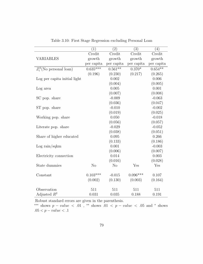
Table 3.10: First Stage Regression excluding Personal Loan
(1) (2) (3) (4)
VARIABLESCreditgrowth
per capita
Creditgrowth
per capita
Creditgrowth
per capita
Creditgrowth
per capita
ZSi (No personal loan) 0.635*** 0.561** 0.370* 0.654**
(0.196) (0.230) (0.217) (0.265)Log per capita initial light 0.002 0.006
(0.004) (0.005)Log area 0.005 0.001
(0.007) (0.008)SC pop. share -0.009 -0.063
(0.036) (0.047)ST pop. share -0.010 -0.002
(0.019) (0.025)Working pop. share 0.050 -0.018
(0.056) (0.057)Literate pop. share -0.029 -0.052
(0.038) (0.051)Share of higher educated 0.095 0.266
(0.133) (0.186)Log rain/sqkm 0.001 -0.003
(0.006) (0.007)Electricity connection 0.014 0.003
(0.016) (0.028)State dummies No No Yes Yes
Constant 0.103*** -0.015 0.096*** 0.107(0.002) (0.130) (0.003) (0.164)
Observation 511 511 511 511Adjusted R2 0.031 0.035 0.188 0.191
Robust standard errors are given in the parenthesis.∗∗∗ shows p − value < .01 , ∗∗ shows .01 < p − value < .05 and ∗ shows.05 < p− value < .1
79

Table 3.11: First Stage Statistics for the Uni-variate Regression excluding PersonalLoanUnderidentification test (Kleibergen-Paap rk LM statistic): 7.655Chi-sq(1) P-val = 0.0057Weak identification test (Cragg-Donald Wald F statistic): 17.467(Kleibergen-Paap rk Wald F statistic): 10.518Stock-Yogo weak ID test critical values: 10% maximal IV size : 16.38Instrumented: Per capita credit growthExcluded instruments: ZS
i (No personal loan)
statistics under-identification and weak identification test are still significant reject-
ing the null hypothesis of both under-identification and weak- identification. The
Kleibergen-Paap rk Wald F-statistics is at 10.518, above the critical value of 10.
Next, we present the corresponding IV regression in Table 3.12. The instrument
ZSi is the predicted credit growth excluding the personal loan component. The first
column of Table 3.12 shows the uni-variate regression of Light growth on the pre-
dicted credit growth. Contrary to our baseline result, we find significant negative
coefficient. Although, the first stage F statistics is at 10.52 which is just above the
critical rule of thumb for a valid instrument. As we include district specific charac-
teristics in the model, the coefficient of the predicted credit growth loses statistical
significance. Additionally the First stage F - statistics fall to 5.94 undermining the
validity of our instrument. We find similar result repeating the model in column (1)
& (2) including state dummies. Column (4) shows the regression including all the
control variables and state dummies. The coefficient of predicted credit growth is
very low at .01 and fail to be significant. The first stage F- statistics is at around 6
and the R2 leaps up to .25.
80
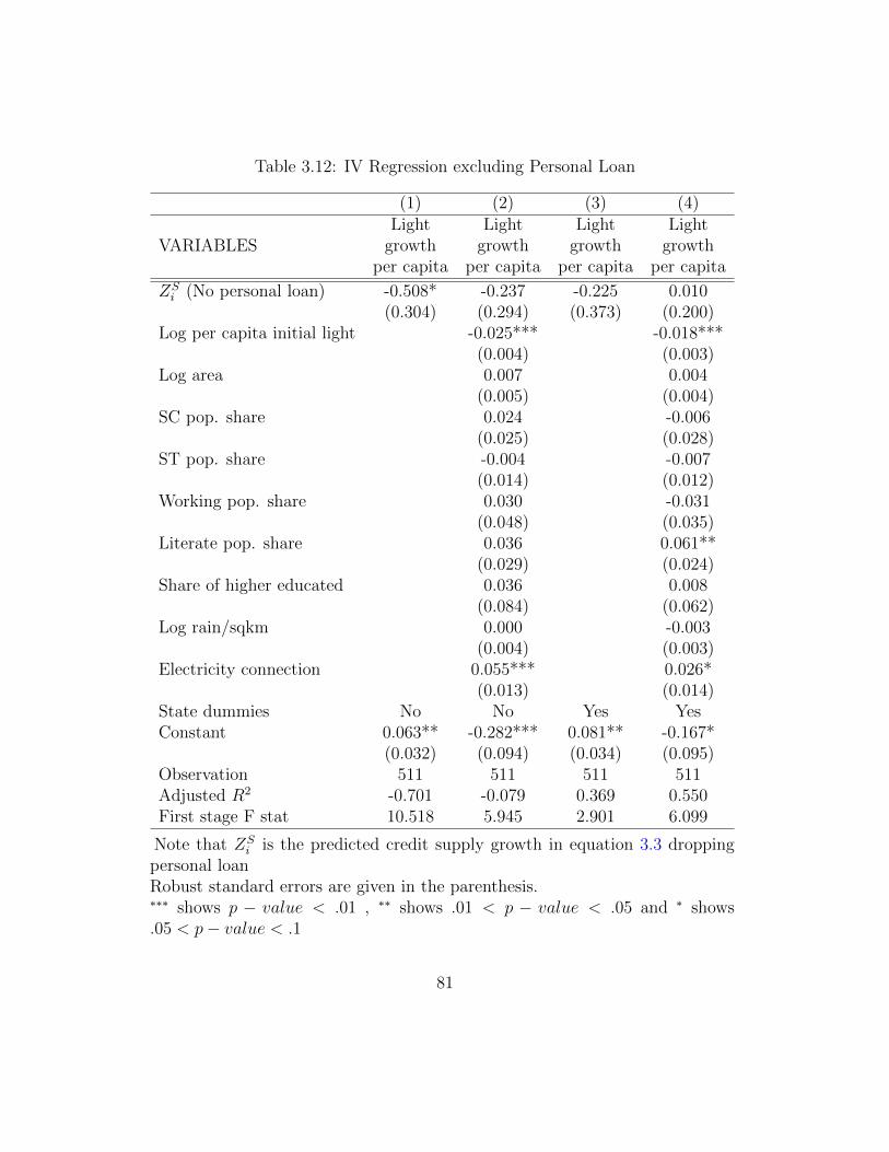
Table 3.12: IV Regression excluding Personal Loan
(1) (2) (3) (4)
VARIABLESLight
growthper capita
Lightgrowth
per capita
Lightgrowth
per capita
Lightgrowth
per capita
ZSi (No personal loan) -0.508* -0.237 -0.225 0.010
(0.304) (0.294) (0.373) (0.200)Log per capita initial light -0.025*** -0.018***
(0.004) (0.003)Log area 0.007 0.004
(0.005) (0.004)SC pop. share 0.024 -0.006
(0.025) (0.028)ST pop. share -0.004 -0.007
(0.014) (0.012)Working pop. share 0.030 -0.031
(0.048) (0.035)Literate pop. share 0.036 0.061**
(0.029) (0.024)Share of higher educated 0.036 0.008
(0.084) (0.062)Log rain/sqkm 0.000 -0.003
(0.004) (0.003)Electricity connection 0.055*** 0.026*
(0.013) (0.014)State dummies No No Yes YesConstant 0.063** -0.282*** 0.081** -0.167*
(0.032) (0.094) (0.034) (0.095)Observation 511 511 511 511Adjusted R2 -0.701 -0.079 0.369 0.550First stage F stat 10.518 5.945 2.901 6.099
Note that ZSi is the predicted credit supply growth in equation 3.3 dropping
personal loanRobust standard errors are given in the parenthesis.∗∗∗ shows p − value < .01 , ∗∗ shows .01 < p − value < .05 and ∗ shows.05 < p− value < .1
81

The instrumental variable regressions excluding personal loan fail to establish
a significant relationship between credit supply growth and growth in economic ac-
tivity. Unlike the previous section, the instrument fails to be valid except for the
uni-variate regression. Even when it is valid, the coefficient of the instrument is
showing an adverse sign at 10% level of significance.
3.6 Conclusion
Our investigation of the effect of credit supply shock on growth of economic
activity has three fold results. First, we find a strong association between credit
growth and economic growth using ordinary least square regression. An 1% increase
in credit is associated with a .1% growth in satellite night light, a measure of economic
activity. Second, we use a shift share approach to estimate predicted growth to
isolate the supply shock in credit from the district specific demand shocks. There is
a strong association between the predicted credit shock and the actual credit shock.
Lastly, we fail to find and association between predicted credit supply shock and
economic growth. We repeated the whole process dropping personal loans to find
similar results.
82

Chapter 4Measuring the Effect ofMisallocation on Productivity inIndian Manufacturing: A GrossOutput Approach
4.1 Introduction
According to World Bank data, the per capita income of US was 34 times higher
than that of India in 2013. Explaining such differences is one of the fundamental
problems in growth economics. Klenow and Rodriguez-Clare [1997], and Hall and
Jones [1999] demonstrated the disparity in Total Factor Productivity (TFP) as the
primary source behind cross country income differences. Another debate in this area
is about the source of TFP differences among rich and poor nations. Banerjee and
Duflo [2005], Restuccia and Rogerson [2008], and Hsieh and Klenow [2009] argued
that in poor countries, some of the TFP differences are generated from misallocation
of resources across firms. In this chapter, we follow the aforementioned notion that
resource misallocation is a primary source of variation in TFP. We include interme-
diate inputs such as raw material, energy and services in the model given by Hsieh
and Klenow [2009] to obtain the extent of misallocation that originates from factor
market distortions in a developing country like India.
There are two known approaches in measuring firm’s output – Value Added and
Gross Output. The former excludes intermediate inputs, whereas the latter includes
them. While measuring physical TFP, one can adopt either of the two approaches.
83

The difference between the two measures of TFP is more pronounced at the firm or
industry level rather than in aggregate output. van der Wiel [1999], Gullickson and
Harper [1999], Hulten [2001], and Cobbold [2003] have demonstrated the benefits of
gross output approach over that of value added. The productivity manual published
by Organisation for Economic Co-operation and Development [2001] concludes that
the gross output approach is more appropriate for productivity measurement be-
cause it reduces productivity measurement bias. Based on these findings we extend
the Hsieh Klenow model to measure productivity using gross output approach by
including raw materials, energy, and service sector intermediate input as factors of
production. The inclusion of these factors separately into production process enables
us to give a more detailed representation of factor misallocation.
TFP, being a residual in the production process, is not observed directly. It
is difficult to measure firm-level TFP as the unit of production varies across the
firms. Therefore, we measure the variation in Total Factor Revenue Productivity
(TFPR), which by definition is the product of output price and physical TFP of a
firm. In the absence of any factor market misallocation, TFPR should be equalized
for all firms within an industry. The intuition behind this claim is as follows: if
a firm has high TFP, the marginal cost as well as the price for that firm will be
proportionally lower compared to a low TFP firm in a particular industry, thus
equalizing the TFPR. We use this intuition given by Restuccia and Rogerson [2008],
and Hsieh and Klenow [2009] to build our empirical results by using data from both
formal and informal manufacturing sector firms in India for the year 2005-06. In
such a developing country, the informal sector plays an extensive role in shaping the
84

economy. The informal manufacturing sector in India consists of around 17 million
firms that provide 82 percent of total employment in that sector. Hence, it seems
rather appropriate to include informal sector data for our empirical analysis.
Our work has the closest resemblance to that of Chatterjee [2011]. To the best of
our knowledge, this is the only available work which also uses gross output approach
in measuring TFPR, and also considers informal firms for India. We extend her work
by including the service sector inputs and the energy inputs in the model separately.
In India, the cost share of service inputs is around 12 percent and that of energy
is around 9 percent for the formal manufacturing sector. Exclusion of these factor
inputs might lead to misleading measurements of output and productivity. We also
include distortion in energy and that in service sector to verify whether some of the
variation in firm-level TFPR is attributed to these factors. We find that there is
very little variation in TFPR due to energy input distortion. The service inputs
misallocation is more pronounced in the dispersion of TFPR.
Furthermore, we decompose factor market distortions by considering each factor
input distortion separately. This exercise facilitates us in distinguishing the level
of misallocation in each factor market and to identify corresponding potential gain
from reallocation. We find that the distortion in the output market and raw material
market explains the lion’s share of the variation in TFPR. Our result is in line with
that of Chatterjee [2011], however, we find the variances of factor distortions to be
larger than that in her result. Another interesting result is that the distortions when
taken from several factor markets together, reduces the variation in TFPR. This
surprising result is the subject of further research.
85

4.2 Related Works
Our work is related to a large body of literature that has accumulated through the last
few decades. Hsieh and Klenow [2009] argue that in a monopolistically competitive
framework, misallocation of the factor markets can result in a large difference in TFP
as well as output among the firms within an industry. For example, a capital market
distortion caused by the disparity in access to cheap credit will result in differences in
the marginal product of capital among firms. Hsieh and Klenow argued that in such
a situation, the aggregate economy will be better off by allocating more capital to the
firm with the higher marginal product of capital. Using firm-level data from India
and China, they calculated the TFP gain from the reallocation of capital, equalizing
TFPR within the industry, to be 30 to 50 percent in China and 40 to 60 percent in
India. We follow the same intuition in our work. We include raw materials, energy,
and service sector inputs as factors of production and find the effect of distortion in
all those inputs on firm level TFPR. Our goal is to find the empirical measurement
of distortion in individual factor markets on aggregate TFPR.
Restuccia and Rogerson [2008] demonstrates the effect of factor distortion on
TFP. They state that the different taxes and policies in firms create disparity in
prices and lead to 30 to 50 percent decrease in output and TFP in developing coun-
tries. Midrigan and Xu [2010] argues that the financial frictions cause variation in
TFP across firms through two channels. In particular, financial friction distorts en-
try decisions and technological adoption of the producers. Furthermore, it creates
disparity in return to capital among the producers. Fernald and Neiman [2010] devi-
ated from standard set up of monopolistic competition to show that in a two-sector
86

economy with heterogeneous financial policies and monopoly power, there will be a
divergence between TFP, measured in terms of quantity and that in terms of real
factor prices.
There is a body of literature based on Hsieh and Klenow framework. Camacho
and Conover [2010] used Hsieh and Klenow methodology to measure the productiv-
ity differences through misallocation in resources for Colombian industries. Taking
USA as the benchmark economy, they found a wide TFPR distribution for Colom-
bia, that implies large resource misallocation across firms. They also calculated the
reallocation of labor and capital among firms would have improved aggregate TFP
by 47 to 55 percent. Another paper by Kalemli-Ozcan and Sørensen [2014] measures
the TFP dispersion through capital misallocation for 10 African countries using the
World Bank enterprise survey data. They argued that access to finance as one of
the main source of substantial capital misallocation. Dias, Dias et al. [2014] extends
Hsieh-Klenow model to include intermediate input and measure TFP disparity tak-
ing firm-level data from Portugal. They consider data from all the sectors of the
economy. Consequently, the endogeneous intermediate input in their model takes
into account goods produced by all the sectors. In India it is rather difficult to find
firm level data for sectors other than manufacturing, thus we take aggregate input
produced by other sectors as exogenously given in our model. Dias et al. found huge
misallocation across industries. According to them, in the absence of misallocation
within industries, there would have been a 48 to 79 percent gain in value added
output during 1996 to 2011.
87

The most closely related work to our research is the paper by Chatterjee [2011],
which tries to extend Hsieh-Klenow framework for both formal and informal manufac-
turing sector of India. Chatterjee also included intermediate input market distortion
in the model as a source of variation in TFP. She assumes that the economy has
an intermediate input aggregated from a fraction of the total production by each
existing firm. the data is taken from ASI for formal firms and NSSO for informal
sector firms, similar to that of our case. As both of these surveys primarily focus on
manufacturing sector firms, the aggregated intermediate input produced from these
firms will take into account only manufacturing sector products. In consequence, she
ignores inputs from other sectors such as energy and services in her model. However,
we consider an aggregated energy and service inputs to be exogenously given in our
model apart from the combined raw material produced by the existing firms. In the
next section, we extend the model of Hsieh and Klenow to measure the degree of
misallocation in the economy.
The rest of this chapter is organized as follows: we present a theoretical model
to show how TFPR is affected by firm level distortion in Section 4.3. The data is
described in Section 4.4. We analyze our empirical results and decomposition of
the variance of TFPR in Section 4.5. In Section 4.6, we construe some relationship
between firm size and misallocation in factor markets. We conclude in Section 4.7.
4.3 Model
We consider a static one period model without uncertainty, used by Hsieh and Klenow
[2009]. We assume that the economy consists of J manufacturing industries indexed
as j = 1, 2, · · · , J . Each industry consists of Nj monopolistically competitive firms
88

indexed as i = 1, 2, · · · , Nj. Each firm produces differentiated product, and thus
has substantial market power. The firms have heterogeneous productivity Aij exoge-
nously given, and an endowment of capital Kij, labor Lij, raw material Mij, energy
Eij, and service sector input Zij. Firms combine the factors together to produce a
good with a Cobb-Douglas production function. The firm’s production function is
as follows
Yij = AijKαKj
ij LαLj
ij MαMj
ij EαEj
ij ZαZj
ij ,
where∑S
αSj = 1 and S ∈ {K,L,M,E, Z}.
We consider only manufacturing sector firms in the model because we could find
data only for manufacturing sector in India for our empirical analysis. For the sim-
plicity of the model, we assume that all raw materials coming from the manufacturing
sector are aggregated in a single raw material M, whereas all energy inputs and ser-
vice sector inputs are aggregated in factor inputs E and Z respectively. We consider
M as endogenously determined whereas energy and service sector inputs along with
capital and labor are exogenously given in our model.
Here, we deviate from the work of Chatterjee [2011], which considers one inter-
mediate input M, has been aggregated combining fractions of production from each
existing firms. As she also studies only the manufacturing firms, this endogeneity
assumption implies that the sole intermediate good regarded in her model consists
only of manufacturing products, thereby ignoring any other sector. On the contrary,
we consider an interdependent structure of different sectors of the economy. There
are other sectors that produce energy and services which are used as intermediate
89

inputs in production process of manufacturing firms. These sectors also use manufac-
turing goods as intermediate inputs in their production. Those intermediate inputs
produced by manufacturing firms that are used in other sectors is considered as a
part of consumption good in our model. We assume that all firms in an industry have
same cost share of factor inputs αSj, but there is variation in factor shares between
the industries.
In this chapter, we measure the misallocation in resources that affect firm level
TFPR. Distortion in an input or output market does not always uniformly increase
(or, decrease) the marginal product of the factors of production (MPF) for all firms.
As firms equalize price with the marginal product of factor inputs, a firm facing
taxes will have higher MPF for service inputs than the firms facing subsidies. The
intuition behind the entire literature based on Hsieh and Klenow (2009) originates
from the hypothesis that the aggregate productivity will be larger if the factors can
be reallocated from lower MPF firms to that of higher MPF firms.
We assume several kinds of factor market distortions in our model. Some ele-
ments that change MPF for all inputs by the same proportion are denoted as output
distortion (τY ij). tax on output of a firm affects all the inputs proportionally, thus
can be identified as an example of output distortion. Moreover, if the distortion
creates a discrepancy in only the marginal product of capital, we call it capital dis-
tortion (τKij) in accordance with Hsieh and Klenow. Similar remarks hold for raw
material distortion (τMij), energy distortion (τEij,) and service sector input distor-
tion (τZij). For an instance, price differentiation in the electricity between small and
large businesses is perceived as energy distortion as it affects only the marginal prod-
90

uct of energy. It is to be noted that we do not consider labor distortion separately,
but that every other distortion affects the respective MPF, relative to the marginal
productivity of labor.
Each firm produces a single good Yij that is to be used both as final consumption
good and as intermediate raw materials. Cij and Xij denote the final consumption
good and intermediate raw material respectively, that are produced by the ith firm
from the jth industry.
Firms face a downward sloping demand schedule that resulted from the assump-
tion of differentiated product environment in a monopolistically competitive market.
So, the industry’s final good appears to be a CES aggregation of all firm’s final goods
represented as,
Yj =
( Nj∑i=1
Y
ρ− 1
ρij
) ρ
ρ− 1
where ρ > 1 is the elasticity of substitution. For simplicity, we assume elasticity
of substitution is the same over all industries. This assumption follows from the
literature. Each industry’s output is sold as consumption good Cj and intermediate
raw material Xj as was the case with firm level output.
We further assume that the market of consumption good and raw material,
produced by each industry, is perfectly competitive. So, the final consumption good
is aggregated from industry level consumption good by a Cobb-Douglas production
function.
91

C =J∏j=1
Cθjj , where
J∑j=1
θj = 1
The intermediate raw material is produced endogenously by aggregating each
industries’ production of raw material, again using a Cobb-Douglas production func-
tion as follows.
M =J∏j=1
Xλjj , where
J∑j=1
λj = 1
In the above two equations, θj and λj are the factor shares of each industry
in total consumption and total intermediate raw material production respectively.
Each firm chooses intermediate raw material from the aggregated M according to
their productivity.
The aggregate quantity of other inputs such as energy E and services Z are
exogenous in our model. Given that, each firm chooses the optimal amount Eij and
Zij based on its production function. The industry aggregates Ej and Zj are given
by the sum over each firm’s usage in that industry.
Now, we try to solve the model for optimal factor resources and output by
maximizing profit for firm, industry, and economy. We assume that the total factor
resources are limited in the manufacturing sector by the aggregate usage of the firms
in the sector. For each S ∈ {K,L,M,E, Z}, we write the aggregate factor resources
92

as in the following equation:
S =J∑j=1
Nj∑i=1
Sij
Next, we solve for the equilibrium to identify the effects of distortion on productivity.
4.3.1 Equilibrium Analysis
In this section, we present a comprehensive equilibrium structure for the firms, the
industries, and the economy. The equilibrium consists of the quantities of the con-
sumption good and the intermediate raw material produced at the firm, industry,
and the aggregate economy level. It also takes into account the optimal amount
of capital, labor, raw material, energy, and services, which are used by each firm.
The input markets and final good markets clear at equilibrium. We now solve the
optimization problems for each market.
• Final Good Problem:
We assume a representative firm produces a final good Y that is used in con-
sumption C and in raw material M for further production. C is produced using the
consumption goods Cj produced by the industries. We assume C to be a numeraire
commodity with unit price P . Likewise, Pj represents the price for industry output
Yj. We do not distinguish between price of final good Cj and raw material Xj, pro-
duced by each industry, on the assumption that both are fractions of the same good,
and are subjected to same cost and market structure. So, the optimization problem
for the final consumption good is given by
93

maxCj
PC −J∑j=1
PjCj (4.1)
subject to
C =J∏j=1
Cjθj (4.2)
• Intermediate Raw Material Problem:
The fraction of the good produced by the representative firm, that used as the
intermediate raw material, is produced using raw materials produced by each in-
dustry. Price of the aggregated intermediate raw material M is given by pm. The
representative firm optimizes the production of M as follows.
maxMj
pmM −J∑j=1
PjXj (4.3)
subject to
M =J∏j=1
Xλjj (4.4)
we solve the final good’s problem from equation 4.1 and 4.2 and the intermediate
raw material’s problem from equation 4.3 and 4.4 to find out the prices set by the
94

representative firms. We get the market clearing price of the final good as
P =J∏j=1
(Pjθj
)θj= 1 (4.5)
and the intermediate raw material’s price as
pm =J∏j=1
(Pjλj
)λj(4.6)
The second equality in equation 4.5 follows from our assumption that C is nu-
meraire good. Both prices are functions of the industry price (Pj) and the share of
each industry in producing the same good (θj and λj, respectively).
• Industry’s Problem:
The final good produced by each industry Yj is used as both final consumption
good Cj and intermediate raw material Xj. We assume that Cj and Xj are fractions
of the same good, and hence, faces the same optimization problem. Furthermore,
Cij and Xij are fraction of firm’s output Yij; therefore, we assume that they are
produced using the same production function, and that they also incur the same
marginal cost. It is safe to assume that the firms charge the same price Pij for both
parts of their output. We represent the industry’s problem as
maxYj
PjYj −J∑j=1
PijYij (4.7)
95

subject to
Yj =
( Nj∑i=1
Y
ρ− 1
ρij
) ρ
ρ− 1 (4.8)
We get the market clearing industry price to be
Ps =
( Nj∑i=1
P 1−ρij
)1/(1−ρ)
(4.9)
• Firm’s Problem:
To allow for factor misallocation in the input and output markets, we consider
several types of distortions. We assume that there exists an output distortion (τY ij)
that affects marginal product of each factor of production by the same proportion.
We also consider capital distortion (τKij), raw material distortion (τMij), energy dis-
tortion (τEij), and service sector input distortion (τZij) that affects marginal prod-
uct of capital, raw material, energy, and service inputs respectively, relative to the
marginal product of labor. Each firm solves the following profit maximization prob-
lem to choose optimal capital, labor, raw material, energy, and service inputs.
maxYij
PijYij(1− τY ij)− wLij − r(1 + τKij)Kij − pm(1 + τMij)Mij
−pe(1 + τEij)Eij − pz(1 + τZij)Zij (4.10)
96

subject to
Yij = AijKαKj
ij LαLj
ij MαMj
ij EαEj
ij ZαZj
ij (4.11)
Solving firm i’s problem,
K∗ij =
(ρ− 1
ρ
)αKj(1− τY ij)PijYij(1 + τKij)r
(4.12a)
L∗ij =
(ρ− 1
ρ
)αLj(1− τY ij)PijYijw
(4.12b)
M∗ij =
(ρ− 1
ρ
)αMj(1− τY ij)PijYij(1 + τMij)pm
(4.12c)
E∗ij =
(ρ− 1
ρ
)αEj(1− τY ij)PijYij(1 + τEij)pe
(4.12d)
Z∗ij =
(ρ− 1
ρ
)αZj(1− τY ij)PijYij(1 + τZij)pz
(4.12e)
Optimal quantities of factor inputs contain both output distortion and distortion
in their respective factor market. Combining the equations 4.12a–4.12e with firm’s
objective function in equation (4.10), we get the market clearing price for each firm
to be
Pij =
(ρ− 1
ρ
)(MC
ε
)(1 + τKij)αKj(1 + τMij)
αMj(1 + τEij)αEj(1 + τZij)
αZj
(1− τY ij)Aij(4.13)
97
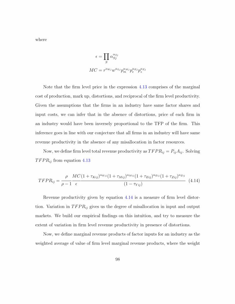
where
ε =∏S
ααSj
Sj
MC = rαKjwαLjpαMjm pαEj
e pαZjz
Note that the firm level price in the expression 4.13 comprises of the marginal
cost of production, mark up, distortions, and reciprocal of the firm level productivity.
Given the assumptions that the firms in an industry have same factor shares and
input costs, we can infer that in the absence of distortions, price of each firm in
an industry would have been inversely proportional to the TFP of the firm. This
inference goes in line with our conjecture that all firms in an industry will have same
revenue productivity in the absence of any misallocation in factor resources.
Now, we define firm level total revenue productivity as TFPRij = PijAij. Solving
TFPRij from equation 4.13
TFPRij =ρ
ρ− 1
MC
ε
(1 + τKij)αKij(1 + τMij)
αMij(1 + τEij)αEij(1 + τZij)
αZij
(1− τY ij)(4.14)
Revenue productivity given by equation 4.14 is a measure of firm level distor-
tion. Variation in TFPRij gives us the degree of misallocation in input and output
markets. We build our empirical findings on this intuition, and try to measure the
extent of variation in firm level revenue productivity in presence of distortions.
Now, we define marginal revenue products of factor inputs for an industry as the
weighted average of value of firm level marginal revenue products, where the weight
98

is taken as share of the firm’s output in the industry, as presented in the following
equation:
MRPSj =PS
Ns∑i=1
(1− τY ij)PijYij(1 + τSij)PjYj
(4.15)
Note that S consists of all factor inputs such as K, L, M, E, and Z. PS denotes
the corresponding factor prices r, w, pm, pe, and pz respectively, and τSij indicate
the corresponding factor distortions. Also note that we did not take labor distortion
implying τLij to be zero.
We define industry level total factor revenue productivity (TFPRj) to be pro-
portional to geometric average of the average marginal revenue products of factor
inputs in the industry (given in equation 4.15).
TFPRj =ρ
ρ− 1
MC
ε
[ 1
Nj∑i=1
(1− τY ij)PijYij(1 + τKij)PjYj
]αKj[ 1
Nj∑i=1
(1− τY ij)PijYijPjYj
]αLj
[ 1
Nj∑i=1
(1− τY ij)PijYij(1 + τMij)PjYj
]αMj[ 1
Nj∑i=1
(1− τY ij)PijYij(1 + τEij)PjYj
]αEj[ 1
Nj∑i=1
(1− τY ij)PijYij(1 + τZij)PjYj
]αZj
(4.16)
99

4.3.2 Allocation of Factors in Industry
We now solve for the allocation of factor resources for each industry. We aggregate
factor resources used by all the firms in an industry using their marginal product to
get the following:
Sj =
Nj∑i=1
Sij = SαSjθj/MRPSj
J∑j=1
αSjθj/MRPSj
(4.17)
Recall that S ∈ {K,L,M,E, Z} and S =∑J
j=1 Sj are aggregate supplies of
factor inputs in the economy. Also recall that θj is the share of each industry in
producing final consumption good. Note that factor accumulations of each industry
is affected by factor distortions only through the corresponding marginal revenue
products. This result is the consequence of the Cobb-Douglas aggregation in industry
level. Combining the industry level factor inputs (4.17) and the revenue productivity
(4.16), we can derive
PjYj = TFPRjKαKj
j LαLj
j MαMj
j EαEj
j ZαZj
j (4.18)
Combining industry price Pj from (4.9) and firm’s price Pij from (4.13) together with
firm level revenue prodictivity from (4.14), we can simplify
Pj =
[ Nj∑i=1
(TFPRij
Aij
)(1−ρ)] 1
1− ρ (4.19)
100
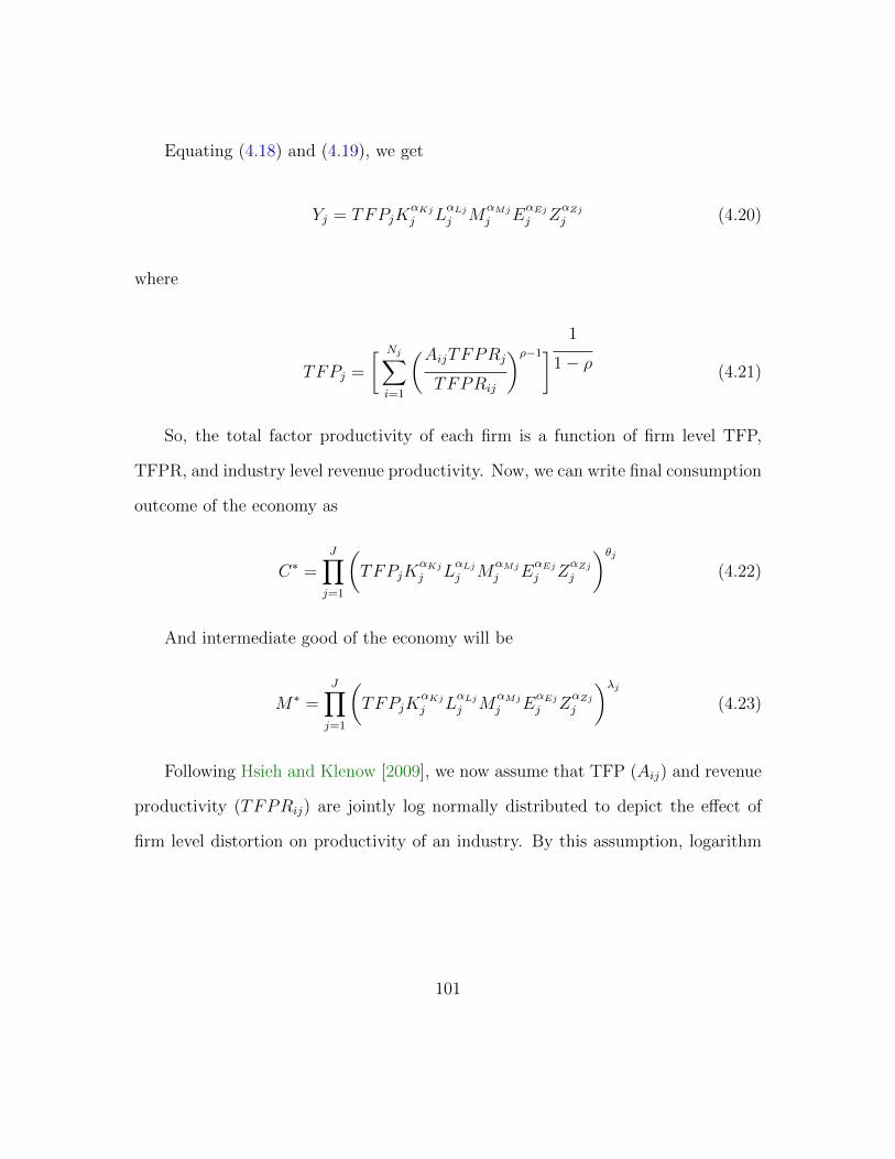
Equating (4.18) and (4.19), we get
Yj = TFPjKαKj
j LαLj
j MαMj
j EαEj
j ZαZj
j (4.20)
where
TFPj =
[ Nj∑i=1
(AijTFPRj
TFPRij
)ρ−1] 1
1− ρ (4.21)
So, the total factor productivity of each firm is a function of firm level TFP,
TFPR, and industry level revenue productivity. Now, we can write final consumption
outcome of the economy as
C∗ =J∏j=1
(TFPjK
αKj
j LαLj
j MαMj
j EαEj
j ZαZj
j
)θj(4.22)
And intermediate good of the economy will be
M∗ =J∏j=1
(TFPjK
αKj
j LαLj
j MαMj
j EαEj
j ZαZj
j
)λj(4.23)
Following Hsieh and Klenow [2009], we now assume that TFP (Aij) and revenue
productivity (TFPRij) are jointly log normally distributed to depict the effect of
firm level distortion on productivity of an industry. By this assumption, logarithm
101

of firm level TFP can be expressed as
log TFPj =1
1− ρlog
( Nj∑i=1
A(ρ−1)ij
)−ρ
2Var(log TFPRij) (4.24)
Equation (4.21) shows that the factor distortions reduce overall productivity of
an industry through the variance of firm level TFPR. On the basis of this finding,
we will now proceed to show how the factor distortions are contributing to firm
level TFPR variation. Note that we consider the number of firms are unaffected by
factor market distortions. This assumption is elaborated in more detail in Hsieh and
Klenow [2009].
4.4 Data
We use data for formal manufacturing sector from the Annual Survey of Industries
(ASI) collected by the Central Statistical Organization of India. ASI is the primary
source of industrial statistics in India, referring to the factories defined in accordance
with the Factories Act 1948. ASI data acts as an annual survey for formal manufac-
turing firms with more than fifty workers and a random one-third sample survey of
firms with more than ten workers (with power) or more than twenty workers (without
power). We use 62nd round of ASI data collected in the year of 2005-06.
We also take into account data for unorganized manufacturing sector collected
by National Sample Survey Organization (NSSO) of India for the year 2005-06. The
NSSO collects firm level data for informal manufacturing sector in India every five
years. The data set includes small manufacturing firms along with some service sector
firms and some unincorporated proprietary firms. These firms are not registered
102

Table 4.1: Informal Firm Distribution
No. of labor No. of firmCumulative %of value added
1 31874 1.62 23734 4.43 9468 6.94 4685 9.15 2601 11.66 1948 17.87 1349 21.88 1054 26.09 732 31.010 648 37.010 to 20 1648 57.420 to 30 327 62.830 to 50 185 73.050 to 100 92 95.0more then 100 61 100.0
under the Factories Act 1948, thus are not included in ASI data. We found that
the data for informal sector consists of a large number of firms that uses one or
two workers. These firms had missing value of most of the variables we take into
consideration. Also, they contribute a very small percentage of the total value added.
Table 4.1 summarizes the distribution of informal firms and corresponding cu-
mulative percentages of the contribution in the total value added, according to the
number of employees. There are over thirty thousand one-employee-firms, which
contributes only 1.6 percent of the total value added and almost none of them had
data for labor and capital. In our analysis, we do not include such firms. We only
consider the informal firms that uses at least six employees, and set the cut off to
be six employees on the basis of a substantial market share of such firms. To keep
the two data set comparable, we only consider the manufacturing industries from
103

Table 4.2: Distribution of Firms: ASI vs NSSOASI Data NSSO Data
No. of employees No. of firms No. of employees No. of firms1 to 10 4663 6 to 10 302610 to 20 7683 10 to 20 160520 to 50 7272 20 to 50 43250 to 100 3838 50 to 100 79100-500 7695 100-500 31
500 and above 2254 500 and above 5
informal sector data that were covered by ASI in its formal counterpart.
Table 4.2 shows the distribution of firms in our analysis. There are around
31 thousand formal sector firms taken from ASI data whereas number of informal
sector firms from NSSO data is around 5 thousand. For our analysis, we had to
drop some observations from both sectors due to missing data. Formal firms consists
of all sizes while informal firms are mostly small. To simplify our analysis, we use
2-digit industry level data developed by National Industrial Classification (NIC). We
consider 23 different industries including food and beverage, hardware, wood, paper,
printing, computer and machinery, and etc. (see table 4.3)
Hsieh and Klenow [2009] used value added method to measure productivity and
distortion in capital and output. They did not incorporate raw material, service or
energy inputs in the production function. We will first replicate their results using
value added method, then extend the model to incorporate intermediate inputs as
factors of production. This extension will lead us to adopt Gross Output Method
instead. We use nominal revenue of the firm as our output variable.
104
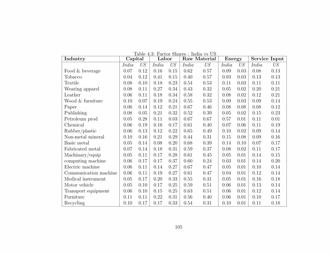
105
Table 4.3: Factor Shares : India vs USIndustry Capital Labor Raw Material Energy Service Input
India US India US India US India US India USFood & beverage 0.07 0.12 0.16 0.15 0.62 0.57 0.09 0.03 0.08 0.13Tobacco 0.04 0.12 0.41 0.15 0.40 0.57 0.03 0.03 0.13 0.13Textile 0.08 0.10 0.18 0.23 0.54 0.53 0.11 0.03 0.11 0.11Wearing apparel 0.08 0.11 0.27 0.34 0.43 0.32 0.05 0.02 0.20 0.21Leather 0.06 0.11 0.18 0.34 0.58 0.32 0.08 0.02 0.12 0.21Wood & furniture 0.10 0.07 0.19 0.24 0.55 0.53 0.09 0.03 0.09 0.14Paper 0.06 0.14 0.12 0.21 0.67 0.46 0.08 0.08 0.08 0.12Publishing 0.08 0.05 0.21 0.32 0.52 0.39 0.05 0.02 0.15 0.23Petroleum prod 0.05 0.28 0.11 0.03 0.67 0.67 0.57 0.01 0.11 0.01Chemical 0.06 0.19 0.16 0.17 0.61 0.40 0.07 0.06 0.11 0.19Rubber/plastic 0.06 0.13 0.12 0.22 0.65 0.49 0.10 0.02 0.09 0.14Non-metal mineral 0.10 0.16 0.21 0.29 0.44 0.31 0.15 0.08 0.09 0.16Basic metal 0.05 0.14 0.08 0.20 0.68 0.39 0.14 0.10 0.07 0.17Fabricated metal 0.07 0.14 0.18 0.31 0.59 0.37 0.08 0.02 0.11 0.17Machinary/equip 0.05 0.11 0.17 0.28 0.61 0.45 0.05 0.01 0.14 0.15computing machine 0.06 0.17 0.17 0.37 0.60 0.24 0.03 0.01 0.14 0.20Electric machine 0.06 0.11 0.14 0.27 0.67 0.47 0.05 0.01 0.10 0.14Communication machine 0.06 0.11 0.19 0.27 0.61 0.47 0.04 0.01 0.12 0.14Medical instrument 0.05 0.17 0.20 0.33 0.55 0.31 0.05 0.01 0.16 0.18Motor vehicle 0.05 0.10 0.17 0.25 0.59 0.51 0.06 0.01 0.13 0.14Transport equipment 0.06 0.10 0.15 0.25 0.63 0.51 0.06 0.01 0.12 0.14Furniture 0.11 0.11 0.22 0.31 0.56 0.40 0.06 0.01 0.10 0.17Recycling 0.10 0.17 0.17 0.33 0.54 0.31 0.10 0.01 0.11 0.18

The variables, other than firm’s revenue, that we use for our analysis are firm’s
industry (2-digit NIC), labor compensation, net book value of fixed capital stock,
rent on capital, intermediate input costs, fuel and energy costs. We assume that
the service input cost is same as the residual cost. We use the labor compensation
including wages, bonuses and benefits to be a proxy for labor input. Capital is
measured by the average of net book value of capital at the beginning and the end
of the year. We deviate from Hsieh and Klenow [2009], Chatterjee [2011] as well as
other previous researches, based on the measurement of the rental cost for capital.
All other literature in this field have taken an exogenous percentage of capital to be
the rental cost, whereas, we measure the same by variables such as rent for machinery,
building, land, interest paid on loan, and etc, which have been taken from the ASI
data for formal sector. For informal firms though, the NSSO data does not explicitly
provide the rent of capital. We measured rental cost from the residual of value
added after subtracting total labor cost. The costs of raw materials, and energy
are calculated explicitly from the cost of inputs of production. Service input costs
consist of transport and communication, insurance charges, license cost, and other
operative expenses.
The elasticity of substitution (ρ) is assumed to be constant in our model. Based
on the previous literature in this field, we take the value of ρ to be equal to 3. In
most part of our empirical analysis, we will use US factor shares for corresponding
industries as a benchmark to identify the effect of distortion on productivity. We took
the factor share data for US industries from Bureau of Economic Analysis (BEA)
governed by US Department of Commerce.
106

4.5 Empirical Analysis
Our identification strategy is similar to that of Hsieh and Klenow [2009] and Chat-
terjee [2011]. We establish our identification of distortions based on the rationale
that in absence of distortion, revenue factor shares of output will be proportional to
the parameters αKj, αLj, αMj, αEj, and αZj in a market with monopolistic competi-
tion. As we assume distortion in factor markets, the revenue shares will give a biased
estimation of the parameters. We can validate this from the first order conditions of
the firms.
fsj =ρ
ρ− 1
pfSij
PijYij
(1 + τSij)
(1− τYij)(4.25)
where fsj = {αKj, αLj, αMj, αEj, αZj} and pf = {r, w, pm, pe, pz}. Also reall that S
consists of all factor inputs and τSijdenotes corresponding distortions.
In presence of distortions, we cannot identify the misallocation in resources sep-
arately from the bias in the parameters. Following Hsieh and Klenow [2009], we take
into account US factor shares for our analysis. The strategy is based on the assump-
tion that US factor market is less distorted than that in India and the technology
used in the industries are same for both the countries. A more detailed discussion on
the assumptions are presented in Chatterjee [2011]. Factor shares for both countries,
described in Table 4.3, represent the average of the cost share for each factor in each
industry.
Figure 4.1 illustrates the bias in the factor share in Indian industries with respect
to US as a benchmark. Any deviation from the 45 degree line shows misallocation
107

Figure 4.1: Factor share for US and India
in the corresponding factor markets in India. We found a similar pattern in capital,
labor and raw material shares presented in Chatterjee [2011]. It is evident from the
diagram that cost shares of capital labor and service input are significantly higher
in US than India, whereas share of raw material and energy are higher in the latter.
Next, we would like to see within industry variation in average revenue per worker
which is measured by average revenue productivity of labor. Figure 4.2 illustrates
108

Figure 4.2: Logarithm of ARPL Distribution
the distribution of logarithm of firm’s Average Revenue Product of Labor (ARPL)
deviated from industry mean, log(ARPLij/ARPLj). We trim 1 percentile from both
end to avoid outliers. The horizontal axis is showing log(ARPLij/ARPLj), whereas
vertical axes measures the density of the firms. There is a substantial variation in
average revenue product of labor within industry. The variance is measured as 3.76.
4.5.1 Value Added vs. Gross Output Approach
Our goal in this section is to measure the variation in firm level TFPR as an indicator
of misallocation in factor market. Our variable of interest is logarithm of firm level
TFPR as a deviation from industry TFPR, log(TFPRij/TFPRj). We will depict
both value added and gross output approach to measure TFPR. First, we try to
replicate the results from Hsieh and Klenow [2009] using value added approach.
They estimated distribution of TFPR taking formal manufacturing sector data for
1987-88 and 1994-95. We repeat their method taking 2005-06 data for both formal
and informal sector. We also illustrate the TFPR distribution using gross output
109
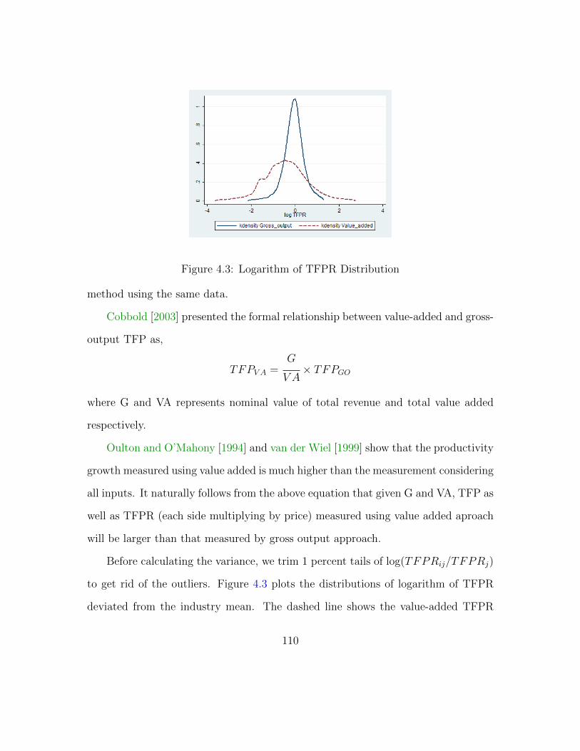
Figure 4.3: Logarithm of TFPR Distribution
method using the same data.
Cobbold [2003] presented the formal relationship between value-added and gross-
output TFP as,
TFPV A =G
V A× TFPGO
where G and VA represents nominal value of total revenue and total value added
respectively.
Oulton and O’Mahony [1994] and van der Wiel [1999] show that the productivity
growth measured using value added is much higher than the measurement considering
all inputs. It naturally follows from the above equation that given G and VA, TFP as
well as TFPR (each side multiplying by price) measured using value added aproach
will be larger than that measured by gross output approach.
Before calculating the variance, we trim 1 percent tails of log(TFPRij/TFPRj)
to get rid of the outliers. Figure 4.3 plots the distributions of logarithm of TFPR
deviated from the industry mean. The dashed line shows the value-added TFPR
110

Table 4.4: Dispersion of Logarithm of TFPRStatistics Value Added Gross OutputSD 0.99 0.4775-25 1.23 0.5190-10 2.45 1.08Note.The variable is log(TFPRsi/TFPRs)
Table 4.5: Dispersion of Logarithm of TFPR in LiteratureStatistics Hsieh-Klenow (1994-95) Chatterjee (2004-05)SD 0.67 0.4975-25 0.81 0.5690-10 1.6 1.19
Note. Column 1 shows dispersion of TFPR estimated byHsiehand Klenow [2009] for 1994-95 data, using value added approach.Column 2 depicts the same estimated by Chatterjee [2011] for2004-05 data using gross output approach.
distribution whereas the solid line shows that of the gross-output approach. The
variation in value added TFPR is much higher than that in gross output TFPR.
Table 4.4 presents the TFPR dispersion statistics in firm level TFPR. Standard
Deviation (SD) in value-added TFPR is around .99 compared to .47, which is the SD
of TFPR using gross-output approach. The difference in both approaches is more
pronounced in estimating variation in TFPR at higher percentile.
Table 4.5 shows the dispersion in logarithm of TFPR in Hsieh and Klenow [2009]
using value added and the same in Chatterjee [2011] using gross output approach.
Our result displays a larger value-added SD than that of Hsieh and Klenow [2009],
who used the same approach with formal sector data from 1994-95. This may be
due to an increase in the overall level of misallocation in the last decade or inclusion
of informal sector in our analysis.
111

Furthermore, we find comparable result with that of Chatterjee [2011] in disper-
sion of gross output TFPR. After inclusion of energy and service sector distortions,
the SD in firm level TFPR has dropped by .02 from an overall .49 depicted in Chat-
terjee with 2004-05 data. The gap between the results is more conspicuous in 75 to
25 and 90 to 10 percentile.
4.5.2 Decomposition of Misallocation
We now turn towards separating out the effect of each component attributing to the
variance of firm level TFPR. Moving forward, only Gross Output approach will be
considered. We took into account several kinds of distortions in input and output
markets. The calculation for each kind as a function of total revenue, cost of inputs
and factor shares is derived from first order conditions of a firm as,
1− τysi =ρ
ρ− 1
wLsi
αLjPsiYsi(4.26a)
1 + τksi =αKj
αLj
wLsi
RKsi
(4.26b)
1 + τmsi =αMj
αLj
wLsi
pmMsi
(4.26c)
1 + τesi =αEj
αLj
wLsi
peEsi(4.26d)
1 + τzsi =αZj
αLj
wLsi
pzZsi(4.26e)
We assumed the labor market to be undistorted. All input market distortions
are estimated relative to labor market. The intuition behind equations 4.26b-4.26e
112

is that in presence of distortion, the input costs relative to labor compensation will
be lower than given by the output elasticity. Equation 4.26a demonstrates that a
deviation of labor share from output elasticity with respect to labor will result in
output distortion.
Figure 4.4: Distribution of log TFPR taking one distortion at a time
113

Next, we would like to find out the distinct effect of each distortion on logarithm
of TFPR deviated from industry mean. In figure 4.4 the solid lines illustrates the
distribution of our variable of interest, taking one factor distortion at a time. The
dashed line represent the actual firm level TFPR distribution taking all distortion
together. The top panel of Figure 4.4 shows TFPR distribution taking either output
or capital distortion. Similarly, middle and bottom panel depict the scenarios with
only material, energy, or service input distortion respectively.
It is perceptible from Figure 4.4 that output and material distortion play the
primary role in dispersion of TFPR within an industry. Energy distortion is almost
negligible, whereas capital and service input distortions also contribute a modest
share in measurement of misallocation.
To give a more elaborate presentation of the above result, we now find the vari-
ance of log(TFPRij/TFPRj). The total misallocation is measured by the following
variance
Var[log[TFPRij
TFPRj
]] = Var(DK +DL +DM +DE +DZ −DY ) (4.27)
where,
DS = αSj log
[(1 + τSij)
Nj∑i=1
(1− τY ij)PijYij(1 + τSij
)PjYj
](4.28)
and DY = log(1− τY ij) (4.29)
114
Recall that S consists of all factor inputs such as K, L, M, E, and Z. αSj denotes
the corresponding factor shares, and τSij indicate the corresponding factor distor-
tions. Also recall that we consider labor market is undistorted implying τLij to be
zero. In the above equations, DS can be inferred as components of each factor input
in the variance of TFPR. Table 4.6 describes the variance and co-variances of each
of the above components.
Variance of the components of equation (4.16) depict the contribution of fac-
tor distortion in explaining the variation in firm level TFPR. As labor is the only
undistorted factor in our analysis, variance of DL measures the benchmark variation
in industry TFPR in presence of only output distortion, multiplied by cost share of
labor. Moreover, Variance of DY determines the variation in firm TFPR attributed
to only output distortion. Dispersion in DY and DM are very high compared to the
overall variance of log(TFPRij/TFPRj) implying that the misallocation is highest
in output and raw material.
Overall variance in log(TFPRij/TFPRj) includes the pairwise covariance be-
tween the components of equation (4.16) as well. It is interesting to note that the
covariance between output and raw material distortions are the highest (.5716). This
result may follow from the fact that in our framework raw material is endogenous,
thus output of one firm is used as raw material to the other.
Figure 4.5 illustrates the cumulative effect of each factor relative to actual TFPR
distribution. The dashed line shows actual TFPR distribution, whereas the solid line
in each block adds distortion one by one. Without any distortion, there would not
have been any distribution of TFPR. We start from only output distortion in the top
115

Table 4.6: Variance DecompositionComponent Variance-CovarianceVar(DK) 0.0472Var(DL) 0.0119Var(DM) 0.3490Var(DE) 0.0048Var(DZ) 0.0345Var(DY ) 1.1203Cov(DK , DL) 0.0030Cov(DK , DM) 0.0346Cov(DK , DE) 0.0029Cov(DK , DZ) 0.0082Cov(DK , DY ) 0.0727Cov(DL, DM) -0.0026Cov(DL, DE) 0.0001Cov(DL, DZ) 0.0001Cov(DL, DY ) 0.0067Cov(DM , DE) 0.0129Cov(DM , DZ) 0.0533Cov(DM , DY ) 0.5716Cov(DE, DZ) 0.0034Cov(DE, DY ) 0.0302Cov(DZ , DY ) 0.1110Var (log(TFPRsi/TFPRs)) 0.2194
Note: The table shows variance and covariancesof the components of log TFPR, where DS, (S ∈{K,L,M,E, Z}) and DY are given by the equation(4.28) and (4.29)
left panel. The solid line in top right panel depicts the TFPR distribution taking
into account both capital and output distortion. The middle left panel considers
output, capital, and raw material distortions together, while middle right panel adds
energy distortion to the distribution. Bottom panel shows all distortion together,
thus coinciding with the actual TFPR distribution.
116

Figure 4.5: Distribution of TFPR Adding one distortion at a time
The intriguing observation from Figure 4.5 is that addition of each factor mar-
ket distortion tend to reduce the variance of TFPR, thus indicating a lower overall
misallocation. This result implies that when we consider more factor input distor-
tions to our model, they are offsetting the effects of each other in describing total
misallocation.
117

4.6 Misallocation and Firm Size
There is a body of literature on the sources of the factor distortions. Banerjee and
Duflo [2005] discovered that capital market distortion might be originated from dis-
parity in the credit policy. Chatterjee [2011] mentions unavailability of raw material
acting as intermediate input distortion. Bhide [2008] shows that in a developing
country like India, electricity connection taken from private and public enterprises
might cause a distortion in energy prices. Hsieh and Klenow [2009] argues that
government policy, specially size restriction might prohibit the firms to achieve the
optimal scale, thus creating an output distortion. They also considered firm size as
an explanation of TFPR dispersion within industry. In this section, we would like
to examine the relationship between firm size and distortion in factor markets.
Table 4.7: Regression of Firm Size on DistortionVariables log of distortions
Output(1)
Capital(2)
Raw material(3)
Energy(4)
Service(5)
log(labor) 0.0752** 0.2741** 0.0440** 0.1900** 0.0765**(0.0048) (0.0063) (0.0079) (0.005) (0.0047)
Industry effect yes yes yes yes yesOwnership effect Yes Yes Yes Yes YesOrganization effect Yes Yes Yes Yes YesRegion effect Yes Yes Yes Yes YesN 41237 44726 45589 47755 47829
Note. The dependent variables in the regressions are logarithm of output andinput (capital, raw material, energy, service respectively) distortions. Standarderrors are given in the parenthesis. ∗∗ shows p− value < .01
Table 4.7 presents coefficient of regression of firm size on the distortions. We
took logarithm of total labor employed as a measure of firm size. Panel (1) takes
logarithm of firm level output distortion to be the regressand. Similarly, dependent
118

variable for (2), (3), (4) and (5) are logarithm of firm level capital, raw material,
energy and service input distortion respectively. We control for industry fixed effects,
ownership type (private, central government owned, state government owned etc.),
type of organization (Individual Proprietorship, partnership, co-operative society,
and etc.) and location of the firm.
We found a positive relationship of firm size with each kind of distortion, which
is in line with the findings of Hsieh and Klenow [2009]. Smaller firms in formal
or informal sector might be able to avoid some policy restrictions unlike their larger
counterparts. Assumption of monopolistic competition includes the provision of mark
up in our model. Though we assumed all firms in an industry to have same mark
up, larger firms might have greater market power and larger mark up which in turn
will create more output distortion as well as raw material distortion. It will be
fascinating to see the effect of firm size on distortion, once we relax the assumption
of same elasticity of substitution within an industry.
4.7 Conclusion
We measure the aggregate misallocation in resources using firm level data from both
formal and informal manufacturing sectors in India for the year 2005-06. We include
energy distortion and service input distortion to extend existing works such as Hsieh
and Klenow [2009] and Chatterjee [2011] . The dispersion in TFPR within each
industry turns out to be substantial, implying misallocation caused by distortion of
factor resources. While energy distortion does not contribute much to the aggregate
misallocation, effect of service sector input distortion is more pronounced. We further
decomposed the variance of TFPR to find out effect of each factor market distortion
119

separately. We discover that output distortion and raw material distortion contribute
the largest share in aggregate misallocation. Reallocation of such factors within the
industries should result in the highest TFP gain. We also uncover a puzzling result
that the inclusion of many factor distortions together offset each other’s effect and
result in a lower aggregate misallocation. Although unexpected, this result may
inspire further research in this field.
120

Chapter 5Concluding RemarksPost-liberalization growth pattern and the driving factors of such growth in India
has inspired a large body of research. In this dissertation, we address three facets
of regional growth, convergence, and productivity variation, in an effort to provide
a supplement to the existing literature.
The second chapter of this dissertation explores the growth pattern and conver-
gence in Indian districts alongside the rural and urban dimension, using radiance
calibrated satellite night light data. We find both absolute and conditional conver-
gence in the districts, primarily driven by the convergence in rural areas. We fail
to find any evidence of convergence in the urban area. Furthermore, we show that
the state specific characteristics explain almost half of the rural as well as overall
growth. On the other hand, among district level initial conditions, human capital
and infrastructure has a role to play in defining the same. However, array of controls
in our study fails to explain much of urban growth.
The third chapter investigates the impact of credit supply shock on economic
growth in districts measured by the same radiance calibrated night light data. The
modified shift-share approach has been used as a strategy of identification. Although
we find strong positive association of credit growth with the growth in economic
activity, the association fails to hold as we separate out the demand side effects
using predicted lending shocks.
The fourth chapter, on the other hand, measures the aggregate misallocation
121

in resources using firm level data from both formal and informal manufacturing
sectors in India for the year 2005-06. The variance decomposition of TFPR displays
that output, and raw material distortion contribute the largest share in aggregate
misallocation.
122

References
Shilpa Aggarwal. Do rural roads create pathways out of poverty? evidence fromindia. Work. Pap., Indian Sch. Bus., Hyderabad, 2015.
Laura Alfaro, Andrew Charlton, and Fabio Kanczuk. Plant-size distribution andcross-country income differences. Technical report, National Bureau of EconomicResearch, 2008.
Mary Amiti and David E Weinstein. How much do bank shocks affect investment?evidence from matched bank-firm loan data. Technical report, National Bureau ofEconomic Research, 2013.
Sam Asher and Paul Novosad. Market access and structural transformation: Evi-dence from rural roads in india. Job Market Paper January, 11:2016, 2016.
Sanghamitra Bandyopadhyay. Twin peaks: distribution dynamics of economicgrowth across indian states. Growth, inequality and poverty: prospects for pro-poor growth, 2004.
Sanghamitra Bandyopadhyay. Chapter 8 convergence club empirics: Evidence fromindian states. In Inequality, Mobility and Segregation: Essays in Honor of JacquesSilber, pages 175–203. Emerald Group Publishing Limited, 2012.
Abhijit V Banerjee and Esther Duflo. Growth theory through the lens of developmenteconomics. Handbook of economic growth, 1:473–552, 2005.
Pranab Bardhan. Awakening giants, feet of clay: Assessing the economic rise ofChina and India. Princeton University Press, 2012.
Robert J Barro. Convergence and modernisation. The Economic Journal, 125(585):911–942, 2015.
Robert J Barro and Xavier Sala-i Martin. Convergence. Journal of political Economy,100(2):223–251, 1992.
Robert J Barro and Xavier Sala-i Martin. Economic growth, 1995. McGraw0Hill,New York, 1995.
Robert J Barro, Xavier Sala-i Martin, Olivier Jean Blanchard, and Robert E Hall.Convergence across states and regions. Brookings papers on economic activity,pages 107–182, 1991.
123

Levon Barseghyan and Riccardo DiCecio. Entry costs, misallocation, and cross-country income and tfp differences. Federal Reserve Bank of St. Louis WorkingPaper, 2009.
Eric Bartelsman, John Haltiwanger, and Stefano Scarpetta. Cross-country differencesin productivity: The role of allocation and selection. The American EconomicReview, 103(1):305–334, 2013.
Ben S Bernanke and Alan S Blinder. The federal funds rate and the channels ofmonetary transmission. The American Economic Review, pages 901–921, 1992.
Anil K Bhargava. The impact of india’s rural employment guarantee on demand foragricultural technology. 2014.
Amar Bhide. What holds back bangalore businesses? Asian Economic Papers, 7(1):120–153, 2008.
Ariel Burstein and Alexander Monge-Naranjo. Foreign know-how, firm control, andthe income of developing countries. Technical report, National Bureau of EconomicResearch, 2007.
Ana Hidalgo Cabrillana. Endogenous capital market imperfections, human capital,and intergenerational mobility. Journal of Development Economics, 90(2):285–298,2009.
Adriana Camacho and Emily Conover. Misallocation and productivity in colombiasmanufacturing industries. 2010.
Francesco Caselli. Accounting for income differences across countries. Handbook ofeconomic growth, 1:679–741, 2005.
Francesco Caselli and Nicola Gennaioli. Credit constraints, competition, and meri-tocracy. Journal of the European Economic Association, 3(2-3):679–689, 2005.
Areendam Chanda and Bibhudutta Panda. Productivity growth in goods and ser-vices across the heterogeneous states of america. Economic Inquiry, 54(2):1021–1045, 2016.
Areendam Chanda and Dachao Ruan. 150 years of worldwide regional income dif-ferences. Technical report, Working Paper, 2015.
Urmila Chatterjee. Resource Allocation and Efficiency in Developing Countries. PhDthesis, University of California, Berkeley, 2011.
124

Gabriel Chodorow-Reich. The employment effects of credit market disruptions:Firm-level evidence from the 2008–9 financial crisis. The Quarterly Journal ofEconomics, 129(1):1–59, 2014.
Hunter Clark, Maxim Pinkovskiy, and Xavier Sala-i Martin. China’s gdp growthmay be understated. Technical report, National Bureau of Economic Research,2017.
Trevor Cobbold. A comparison of gross output and value-added methods of pro-ductivity estimation. Productivity Commission Research Memorandum, Canberra,2003.
Samarjit Das. The convergence debate and econometric approaches: Evidence fromindia. 2012.
Samarjit Das, Chetan Ghate, and Peter E Robertson. Growth, geography, andthe iron law: Understanding divergence across indian districts. Technical report,Indian Statistical Institute, New Delhi, India, 2013.
Samarjit Das, Chetan Ghate, and Peter E Robertson. Remoteness, urbanization,and india’s unbalanced growth. World Development, 66:572–587, 2015.
Daniel Dias, Carlos Robalo Marques, and Christine Richmond. Misallocation andproductivity in the lead up to the eurozone crisis. Technical report, 2014.
Sean Dougherty, Richard Herd, Thomas Chalaux, and Abdul Erumban. India’sgrowth pattern and obstacles to higher growth. 2008.
Steven N Durlauf and Danny T Quah. The new empirics of economic growth. Hand-book of macroeconomics, 1:235–308, 1999.
Steven N Durlauf, Paul A Johnson, and Jonathan RW Temple. Growth econometrics.Handbook of economic growth, 1:555–677, 2005.
Christopher D Elvidge, Kimberly E Baugh, John B Dietz, Theodore Bland, Paul CSutton, and Herbert W Kroehl. Radiance calibration of dmsp-ols low-light imagingdata of human settlements. Remote Sensing of Environment, 68(1):77–88, 1999.
Shenggen Fan, Peter Hazell, and Sukhadeo Thorat. Government spending, growthand poverty in rural india. American Journal of Agricultural Economics, 82(4):1038–1051, 2000.
125

John Fernald and Brent Neiman. Growth accounting with misallocation: Or, do-ing less with more in singapore. Technical report, National Bureau of EconomicResearch, 2010.
Subhashis Gangopadhyay and SK Shanthi. Domestic financial sector reforms. 2012.
Peter Ganong and Daniel Shoag. Why has regional income convergence in the usdeclined? 2013.
Nicola Gennaioli, Rafael La Porta, Florencio Lopez-de Silanes, and Andrei Shleifer.Human capital and regional development. Technical report, National Bureau ofEconomic Research, 2011.
Nicola Gennaioli, Rafael La Porta, Florencio Lopez De Silanes, and Andrei Shleifer.Growth in regions. Journal of Economic growth, 19(3):259–309, 2014.
Chetan Ghate. Understanding divergence in india: a political economy approach.Journal of Economic Policy Reform, 11(1):1–9, 2008.
Chetan Ghate. The oxford handbook of the indian economy. Oxford University Press,2012.
Chetan Ghate and Stephen Wright. The “v-factor”: Distribution, timing and corre-lates of the great indian growth turnaround. Journal of Development Economics,99(1):58–67, 2012.
Douglas Gollin, Remi Jedwab, and Dietrich Vollrath. Urbanization with and withoutindustrialization. Journal of Economic Growth, 21(1):35–70, 2016.
Michael Greenstone, Alexandre Mas, and Hoai-Luu Nguyen. Do credit market shocksaffect the real economy? quasi-experimental evidence from the great recession and‘normal’ economic times. Technical report, National Bureau of Economic Research,2014.
William Gullickson and Micahel J Harper. Possible measurement bias in aggregateproductivity growth. Monthly Lab. Rev., 122:47, 1999.
Nezih Guner, Gustavo Ventura, and Yi Xu. Macroeconomic implications of size-dependent policies. Review of Economic Dynamics, 11(4):721–744, 2008.
Robert E Hall and Charles I Jones. Why do some countries produce so much moreoutput per worker than others? Technical report, National bureau of economicresearch, 1999.
126

J Vernon Henderson, Adam Storeygard, and David N Weil. Measuring economicgrowth from outer space. The American Economic Review, 102(2):994–1028, 2012.
J Vernon Henderson, Tim L Squires, Adam Storeygard, and David N Weil. Theglobal spatial distribution of economic activity: Nature, history, and the role oftrade. Technical report, National Bureau of Economic Research, 2016.
Chang tai Hsieh and Peter J. Klenow. Misallocation and Manufacturing tfp in chinaand india. Quarterly Journal of Economics, pages 1403–1448, 2009.
Charles R Hulten. Total factor productivity: a short biography. In New developmentsin productivity analysis, pages 1–54. University of Chicago Press, 2001.
Clement Imbert and John Papp. Labor market effects of social programs: Evidencefrom india’s employment guarantee. American Economic Journal: Applied Eco-nomics, 7(2):233–263, 2015.
Rajkamal Iyer, Jose-Luis Peydro, Samuel da Rocha-Lopes, and Antoinette Schoar.Interbank liquidity crunch and the firm credit crunch: Evidence from the 2007–2009 crisis. Review of Financial studies, 27(1):347–372, 2014.
Gabriel Jiminez, Atif R Mian, Jose-Luis Peydro, and Jesus Saurina Salas. The realeffects of the bank lending channel. 2014.
Charles I Jones. Misallocation, economic growth, and input-output economics. Tech-nical report, National Bureau of Economic Research, 2011.
Dale W Jorgenson, Mun S Ho, and Kevin J Stiroh. Growth of us industries andinvestments in information technology and higher education. Economic SystemsResearch, 15(3):279–325, 2003.
Sebnem Kalemli-Ozcan and Bent E Sørensen. Misallocation, property rights, andaccess to finance: evidence from within and across africa. In African Successes:Modernization and Development. University of Chicago Press, 2014.
Asim Ijaz Khwaja and Atif Mian. Tracing the impact of bank liquidity shocks:Evidence from an emerging market. The American Economic Review, 98(4):1413–1442, 2008.
Peter Klenow and Andres Rodriguez-Clare. The neoclassical revival in growth eco-nomics: Has it gone too far? In NBER Macroeconomics Annual 1997, Volume 12,pages 73–114. MIT Press, 1997.
127

Peter J Klenow and Andres Rodriguez-Clare. Externalities and growth. Handbookof economic growth, 1:817–861, 2005.
Stefan Klonner and Christian Oldiges. Can an employment guarantee alleviatepoverty? evidence from india’s national rural employment guarantee act. Draftpaper, University of Heidelberg, 2013.
Melanie Krause and Richard Bluhm. Top lights-bright spots and their contributionto economic development. 2016.
Utsav Kumar and Arvind Subramanian. Growth in india’s states in the first decadeof the 21st century: four facts. Economic & Political Weekly, 47(3):49, 2012.
Somik V Lall. Infrastructure and regional growth, growth dynamics and policyrelevance for india. The Annals of Regional Science, 41(3):581–599, 2007.
N Gregory Mankiw, David Romer, and David N Weil. A contribution to the empiricsof economic growth. Technical report, National Bureau of Economic Research,1990.
N Gregory Mankiw, David Romer, and David N Weil. A contribution to the empiricsof economic growth. The quarterly journal of economics, 107(2):407–437, 1992.
Therese J McGuire and Timothy J Bartik. Who benefits from state and local eco-nomic development policies?, 1992.
Charlotta Mellander, Jose Lobo, Kevin Stolarick, and Zara Matheson. Night-timelight data: A good proxy measure for economic activity? PloS one, 10(10):e0139779, 2015.
Virgiliu Midrigan and Daniel Yi Xu. Finance and misallocation: Evidence fromplant-level data. Technical report, National Bureau of Economic Research, 2010.
Mary O’Mahony and Marcel P Timmer. Output, input and productivity measuresat the industry level: The eu klems database*. The Economic Journal, 119(538):F374–F403, 2009.
Organisation for Economic Co-operation and Development. Measuring Productivity:Measurement of Aggregate and Industry-level Productivity Growth: OECD Manual.Organisation for Economic Co-operation and Development, 2001.
Nicholas Oulton and Mary O’Mahony. Productivity and growth. Cambridge Books,1994.
128

Arvind Panagariya. India: The emerging giant. Oxford University Press, 2008.
Daniel Paravisini, Veronica Rappoport, Philipp Schnabl, and Daniel Wolfenzon. Dis-secting the effect of credit supply on trade: Evidence from matched credit-exportdata. The Review of Economic Studies, 82(1):333–359, 2015.
Rafael La Porta and Andrei Shleifer. The unofficial economy and economic develop-ment. Technical report, National Bureau of Economic Research, 2008.
Edward C Prescott. Lawrence r. klein lecture 1997: Needed: A theory of total factorproductivity. International economic review, pages 525–551, 1998.
Diego Restuccia and Richard Rogerson. Policy distortions and aggregate productivitywith heterogeneous establishments. Review of Economic Dynamics, 11(4):707–720,2008.
SL Shetty. Growth of sdp and structural changes in state economies: Interstatecomparisons. Economic and Political Weekly, pages 5189–5200, 2003.
Nirvikar Singh, Jake Kendall, RK Jain, and Jai Chander. Regional inequality inindia in the 1990s: A district-level view. Technical report, Working Papers, UCSanta Cruz Economics Department, 2013.
Tapen Sinha and Dipendra Sinha. No virginia, states in india are not converging.International Indian Economic Association, Working Paper, (2000-09):01, 2000.
Christopher Small, Christopher D Elvidge, Deborah Balk, and Mark Montgomery.Spatial scaling of stable night lights. Remote Sensing of Environment, 115(2):269–280, 2011.
MS Sriram. Inclusive finance india report 2015. New Delhi, Access DevelopmentServices in Association with Sage Publications India Pvt. Ltd. This is referred toas IFI Report, 2015.
Adam Storeygard. Farther on down the road: transport costs, trade and urbangrowth in sub-saharan africa. The Review of Economic Studies, page rdw020,2016.
Arvind Subramanian. India’s turn: understanding the economic transformation.OUP Catalogue, 2009.
HP van der Wiel. Sectoral labour productivity growth. Research Memorandum,(158), 1999.
129

Xiaobo Zhang and Shenggen Fan. How productive is infrastructure? a new approachand evidence from rural india. American Journal of Agricultural Economics, 86(2):492–501, 2004.
Naijun Zhou, Klaus Hubacek, and Mark Roberts. Analysis of spatial patterns ofurban growth across south asia using dmsp-ols nighttime lights data. AppliedGeography, 63:292–303, 2015.
Laura Zimmermann. Why guarantee employment? evidence from a large indianpublic-works program. Unpublished manuscript, 2013.
Daniel Ziskin, Kimberly Baugh, Feng-Chi Hsu, and Christopher D Elvidge. Meth-ods used for the 2006 radiance lights. Proceedings of the Asia-Pacific AdvancedNetwork, 30:131–142, 2010.
130

Appendix AData Description
Table D1: Data DescriptionVariable Description Source
Log Initial Lightper capita
Logarithm of radiance calibrated satellitenight lights data for 2000 per unitof population.
National GeophysicalData Center
Log Initial Rural Lightper capita
Logarithm of Radiance calibrated satellitenight lights data for 2000 per unitof population, when the Digital numbervalue of two contiguous pixels areless than 12.
National GeophysicalData Center
Log Initial Urban Lightper capita
Logarithm radiance calibrated satellitenight lights data for 2000 per unitof population, when the Digital numbervalue of two contiguous pixelsare more than 12.
National GeophysicalData Center
Night Lights Growthper capita
Per capita radiance calibrated NightTime Light growth over 2000-2010,we also used 2000-05 and 2005-10growth for various regressions.
National GeophysicalData Center
Rural Night LightsGrowth per capita
Radiance calibrated night lightsgrowth Per capita if the DN value oftwo contiguous pixel are less than 12.
National GeophysicalData Center
Urban night lightsgrowth per capita
Radiance calibrated Night Lightsgrowth Per capita if the DN value oftwo contiguous pixel are more than 12.
National GeophysicalData Center
131

Table D1: Data Description (continued)Variable Description Source
Rural Percent Percent of rural popultaionCensus of India2001
Overall Popul-ation Density
Overall population per 100000 square kmCensus of India2002
SC Pop.Share
Share of scheduled castpopulation in total populationcollected for rural and urban areas separately
Census of India2000
ST Pop.Share
Share of scheduled tribepopulation in total populationcollected for rural and urban areas separately
Census of India2000
WorkingPop. Share
Share of working populationin total populationcollected for rural and urban areas separately
Census of India2000
LiteratePop. Share
Share of literate populationin total populationcollected for rural and urban areas separately
Census of India2000
Higher Edu.Share
Share of population withhigher secondary andtertiary educationcollected for rural and urban areas separately
Census of India2000
Log Net IrrigatedArea
Logarithm of net land irrigatedland area (per million population)divided by district population
Das and Ghate& Robertson (2015)
Log HH withPaved Roads
Logarithm of the percentage ofhouseholds connected by paved roads
Das and Ghate& Robertson (2015)
132
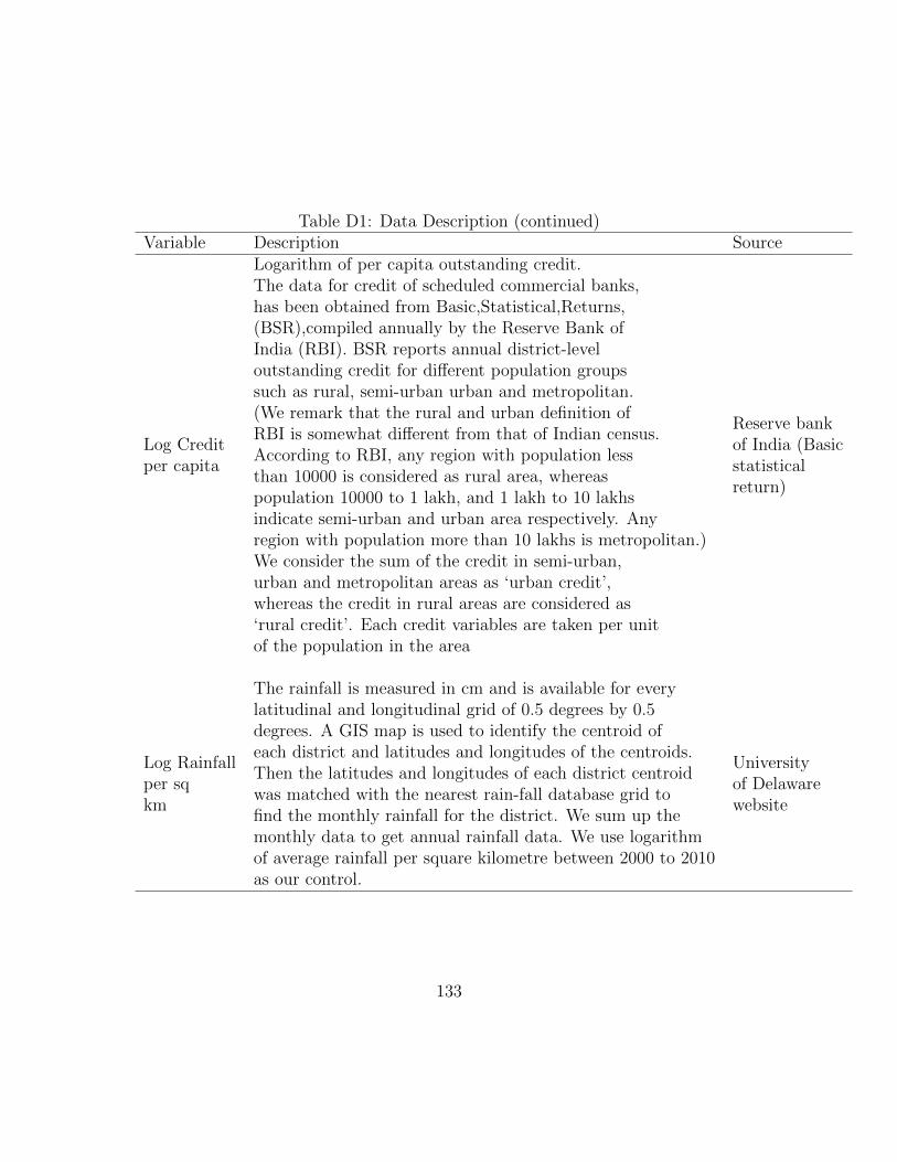
Table D1: Data Description (continued)Variable Description Source
Log Creditper capita
Logarithm of per capita outstanding credit.The data for credit of scheduled commercial banks,has been obtained from Basic,Statistical,Returns,(BSR),compiled annually by the Reserve Bank ofIndia (RBI). BSR reports annual district-leveloutstanding credit for different population groupssuch as rural, semi-urban urban and metropolitan.(We remark that the rural and urban definition ofRBI is somewhat different from that of Indian census.According to RBI, any region with population lessthan 10000 is considered as rural area, whereaspopulation 10000 to 1 lakh, and 1 lakh to 10 lakhsindicate semi-urban and urban area respectively. Anyregion with population more than 10 lakhs is metropolitan.)We consider the sum of the credit in semi-urban,urban and metropolitan areas as ‘urban credit’,whereas the credit in rural areas are considered as‘rural credit’. Each credit variables are taken per unitof the population in the area
Reserve bankof India (Basicstatisticalreturn)
Log Rainfallper sqkm
The rainfall is measured in cm and is available for everylatitudinal and longitudinal grid of 0.5 degrees by 0.5degrees. A GIS map is used to identify the centroid ofeach district and latitudes and longitudes of the centroids.Then the latitudes and longitudes of each district centroidwas matched with the nearest rain-fall database grid tofind the monthly rainfall for the district. We sum up themonthly data to get annual rainfall data. We use logarithmof average rainfall per square kilometre between 2000 to 2010as our control.
Universityof Delawarewebsite
133

Table D2: Reform Project Data DescriptionVariable Description Sources
NREGAExpenditureper capita
Average labor and material expenditure ofNREGA per unit of rural population. Thepublic data portal of MGNREGA showsphysical and monetary variables reportedby the districts to MoRD. We use the datafrom 2006, the year of introduction of the programto 2010.
NREGAWebsite(mnregaweb4.nic.in)
PMGSYExpenditureper capita
Average sanctioned expenditure on rural roadproject per unit of rural population.The data for PMGSY has been taken fromOnline Management and Monitoring System(OMMS). OMMS is used in program tracking andimplementation of the program which provides theadministrative records of the actual program.The OMMS reports district level yearly summaryof number of road built, habitation covered, lengthof total road and LSB (Long Spanning Bridge)construction, and total expenditure in the projects.
OMMSWebsite(omms.nic.in)
RGGVYExpenditureper capita
Average sanctioned expenditure per capita ruralpopulation till the year 2011 per unit of rural population.The DDUGJY website reports plan-wise physical andfinancial progress for districts under RGGVY over tenth,eleventh and twelfth five year plan. The data reportsimplementation agency fund sanction and releasedate along with the amount, number of villages coveredfor both electrification and intense electrification, andnumber of BPL households which are providedwith electricity under the program.
DDUGJYWebsite(www.ddugjy.gov.in)
134

VitaSujana Kabiraj was born in India in 1986. She obtained her Bachelor’s degree in
Economics from the University of Calcutta in 2008. Later, she obtained her first
Master’s degree from the Delhi School of Economics in 2010, and her second Mas-
ter’s degree from the Louisiana State University in 2014, both in Economics. During
her stay at LSU, she worked as a teaching assistant and a primary instructor in
the Department of Economics teaching Principles of Microeconomics, Principles of
Macroeconomics, and Money, Banking and Financial Market. Sujana’s primary re-
search interest includes economic growth, regional economics, convergence, and the
Indian economy. Her doctoral work’s emphasis is on investigating the regional growth
pattern, convergence, and productivity in India.
135