essays on supply chain management with model uncertainty

Essays on Supply Chain Management with Model Uncertainty

by

Mengshi Lu

A dissertation submitted in partial satisfaction of the

requirements for the degree of

Doctor of Philosophy

in

Engineering – Industrial Engineering and Operations Research

in the

Graduate Division

of the

University of California, Berkeley

Committee in charge:

Professor Zuo-Jun Shen, ChairProfessor Andrew Lim

Professor Candace YanoProfessor Bin Yu

Spring 2014


Copyright 2014by

Mengshi Lu

1

Abstract


by

Mengshi Lu

Doctor of Philosophy in Engineering – Industrial Engineering and Operations Research

University of California, Berkeley

Professor Zuo-Jun Shen, Chair

Traditional supply chain management models typically require complete model informa-tion, including structural relationships (e.g., how pricing decisions affect customer demand),probabilistic distributions, and parameters. However, in practice, the model informationmay be uncertain. My dissertation research seeks to address model uncertainty in supplychain management problems using data-driven and robust methods. Incomplete informa-tion typically comes in two forms, namely, historical data and partial information. Whenhistorical data are available, data-driven methods can be used to obtain decisions directlyfrom data, instead of estimating the model information and then using these estimates tofind the optimal solution. When partial information is available, robust methods considerall possible scenarios and make decisions to hedge against the worst-case scenario effectively,instead of making simplified assumptions that could lead to significant loss.

Chapter 1 provides an overview of model uncertainty in supply chain management, anddiscusses the limitations of the traditional methods. The main part of the dissertation ison the application of data-driven and robust methods to three widely-studied supply chainmanagement problems with model uncertainty.

Chapter 2 studies the reliable facility location problem where the joint-distribution of fa-cility disruptions is uncertain. For this problem, usually, only partial information in the formof marginal facility disruption probabilities is available. Most existing models require theassumption that the disruptions at different locations are independent of each other. How-ever, in practice, correlated disruptions are widely observed. We present a model that allowsdisruptions to be correlated with an uncertain joint distribution, and apply distributionally-robust optimization to minimize the expected cost under the worst-case distribution withthe given marginal disruption probabilities. The worst-case distribution has a practical in-terpretation, and its sparse structure allows us to solve the problem efficiently. We findthat ignoring disruption correlation could lead to significant loss. The robust method cansignificantly reduce the regret from model misspecification. It outperforms the traditionalapproach even under very mild correlation. Most of the benefit of the robust model can becaptured at a relatively small cost, which makes it easy to implement in practice.

2

Chapter 3 studies the pricing newsvendor problem where the structural relationship be-tween pricing decisions and customer demand is unknown. Traditional methods for thisproblem require the selection of a parametric demand model and fitting the model usinghistorical data, while model selection is usually a hard problem in itself. Furthermore,most of the existing literature on pricing requires certain conditions on the demand model,which may not be satisfied by the estimates from data. We present a data-driven approachbased only on the historical observations and the basic domain knowledge. The conditionaldemand distribution is estimated using non-parametric quantile regression with shape con-straints. The optimal pricing and inventory decisions are determined numerically using theestimated quantiles. Smoothing and kernelization methods are used to achieve regulariza-tion and enhance the performance of the approach. Additional domain knowledge, such asconcavity of demand with respect to price, can also be easily incorporated into the approach.Numerical results show that the data-driven approach is able to find close-to-optimal solu-tions. Smoothing, kernelization, and the incorporation of additional domain knowledge cansignificantly improve the performance of the approach.

Chapter 4 studies inventory management for perishable products where a parameter ofthe demand distribution is unknown. The traditional separated estimation-optimizationapproach for this problem has been shown to be suboptimal. To address this issue, anintegrated approach called operational statistics has been proposed. We study several im-portant properties of operational statistics. We find that the operational statistics approachis consistent and guaranteed to outperform the traditional approach. We also show that thebenefit of using operational statistics is larger when the demand variability is higher. Wethen generalize the operational statistics approach to the risk-averse newsvendor problemunder the conditional value-at-risk (CVaR) criterion. Previous results in operational statis-tics can be generalized to maximize the expectation of conditional CVaR. In order to modelrisk-aversion to both the uncertainty in demand sampling and the uncertainty in future de-mand, we introduce a new criterion called the total CVaR, and find the optimal operationalstatistic for this new criterion.

i

To my parents

ii

Contents

Contents ii

List of Figures iv

List of Tables v

1 Model Uncertainty in Supply Chain Management 1

2 Reliable Facility Location Design with Distributional Uncertainty 42.1 Introduction . . . . . . . . . . . . . . . . . . . . . . . . . . . . . . . . . . . . 42.2 Literature Review . . . . . . . . . . . . . . . . . . . . . . . . . . . . . . . . . 62.3 Model and Formulation . . . . . . . . . . . . . . . . . . . . . . . . . . . . . . 92.4 Numerical Results . . . . . . . . . . . . . . . . . . . . . . . . . . . . . . . . . 142.5 Extensions to Other Reliable Facility Location Problems . . . . . . . . . . . 242.6 Summary and Future Directions . . . . . . . . . . . . . . . . . . . . . . . . . 26

3 Joint Pricing-Inventory Management with Structural Uncertainty 283.1 Introduction . . . . . . . . . . . . . . . . . . . . . . . . . . . . . . . . . . . . 283.2 Literature Review . . . . . . . . . . . . . . . . . . . . . . . . . . . . . . . . . 303.3 A Data-Driven Approach Based on Isotonic Quantile Regression . . . . . . . 333.4 Smoothing, Concavity Constraint and Kernelization . . . . . . . . . . . . . . 403.5 Numerical Experiments . . . . . . . . . . . . . . . . . . . . . . . . . . . . . . 503.6 Summary and Future Directions . . . . . . . . . . . . . . . . . . . . . . . . . 53

4 Inventory Management for Perishable Goods with Parameter Uncertainty 544.1 Introduction . . . . . . . . . . . . . . . . . . . . . . . . . . . . . . . . . . . . 544.2 Literature Review . . . . . . . . . . . . . . . . . . . . . . . . . . . . . . . . . 554.3 Background on Operational Statistics . . . . . . . . . . . . . . . . . . . . . . 574.4 Properties of Operational Statistics . . . . . . . . . . . . . . . . . . . . . . . 584.5 Operational Statistics under Risk Aversion . . . . . . . . . . . . . . . . . . . 634.6 Summary and Future Directions . . . . . . . . . . . . . . . . . . . . . . . . . 67

A Proofs 68

iii

B Data and Supplementary Results 78B.1 Severe Weather Hazard Data for the Supply Chain Design Example . . . . . 78B.2 Selected Reliable Facility Location Results Using the 88-Node Data Set . . . 78

Bibliography 81

iv

List of Figures

2.1 48-hour impact probability forecast of Hurricane Sandy at the time of its landfall(NOAA, 10-29-2012) . . . . . . . . . . . . . . . . . . . . . . . . . . . . . . . . . 5

2.2 The optimal design under independent disruptions (Design I) . . . . . . . . . . 152.3 The optimal design under worst-case correlated disruptions (Design R) . . . . . 162.4 Impact of important factors on expected regret . . . . . . . . . . . . . . . . . . 202.5 Expected cost under different degrees of disruption correlation . . . . . . . . . 212.6 Benefit and cost of the robust design with different weights . . . . . . . . . . . 222.7 Percentage of maximum benefit captured and maximum cost incurred by different

weights . . . . . . . . . . . . . . . . . . . . . . . . . . . . . . . . . . . . . . . . 23

3.1 Examples of isotonic quantile regression estimates . . . . . . . . . . . . . . . . 373.2 Quantile path and breakpoints in parametric programming . . . . . . . . . . . 383.3 Number of breakpoints in isotonic quantile regression . . . . . . . . . . . . . . . 393.4 Estimated optimal inventory level, expected profit function, and optimal price . 403.5 Quantile path and breakpoints using smoothing . . . . . . . . . . . . . . . . . . 423.6 Improved data-driven solutions using smoothing . . . . . . . . . . . . . . . . . 423.7 Cross validation risk of different smoothing parameters . . . . . . . . . . . . . . 443.8 Quantile path and breakpoints with concavity constraint . . . . . . . . . . . . . 453.9 Improved data-driven solutions with concavity constraint . . . . . . . . . . . . 463.10 Quantile path and breakpoints using kernelization . . . . . . . . . . . . . . . . 493.11 Improved data-driven solutions using kernelization . . . . . . . . . . . . . . . . 49

4.1 Comparison of operational statistics and separated estimation-optimization solu-tions (exponential distribution) . . . . . . . . . . . . . . . . . . . . . . . . . . . 61

4.2 Comparison of the optimality gaps for the operational statistics and separatedestimation-optimization approaches (exponential distribution) . . . . . . . . . . 61

4.3 Impact of demand coefficient of variation on the benefit of operational statistics(shifted exponential distribution) . . . . . . . . . . . . . . . . . . . . . . . . . . 62

4.4 Total CVaR achieved by operational statistics and separated estimation-optimization 66

v

List of Tables

2.1 Summary of literature on reliable facility location . . . . . . . . . . . . . . . . . 72.2 Optimal location designs of the two models . . . . . . . . . . . . . . . . . . . . 162.3 Comparison of the performance of the two designs . . . . . . . . . . . . . . . . 162.4 Levels for important factors . . . . . . . . . . . . . . . . . . . . . . . . . . . . . 182.5 Selected results for the 49-node data set . . . . . . . . . . . . . . . . . . . . . . 19

3.1 Summary of the numerical experiment results . . . . . . . . . . . . . . . . . . . 513.2 Summary of the numerical experiment results with demand concavity . . . . . 52

B.1 Estimated marginal disruption probability for the supply chain design example. 79B.2 Selected results for the 88-node data set. . . . . . . . . . . . . . . . . . . . . . . 80

vi

Acknowledgments

I am deeply indebted to my advisor, Professor Zuo-Jun “Max” Shen, for his guidance,encouragement, and support. He is not only a great research advisor, but also a great mentor.His advice on research and academic career has been invaluable to me. I would also like tothank my dissertation committee members, Professor Andrew Lim, Professor Candace Yano,and Professor Bin Yu. My research benefited greatly from their expertise. Their helpfulcomments and suggestions significantly improved the exposition of my dissertation. I amalso grateful to Professor George Shanthikumar whose research in operations managementunder model uncertainty inspired me to focus my research in this area. As a PhD student,I spent one year conducting research at the Hewlett Packard Laboratories. I would like tothank Dr. Kemal Guler for being a great mentor and a cordial friend, and Professor PinNg for his guidance on quantile regression. I am also grateful to Dr. Fereydoon Safai forsupporting my research at the Hewlett Packard Laboratories.

I would also like to thank the other IEOR faculty members, especially Professor Ying-JuChen, for his advice on my research, and Professor Rhonda Righter, Professor Lee Schruben,and Professor Jon Burgstone, for their help with my teaching. I am also very thankful tothe IEOR staff, especially Mr. Michael Campbell, Ms. Anayancy Paz, and Mr. Jay Sparks.I had an amazing time while living in Berkeley. I would like to thank my dear friends,including Yong, Ye, Tianhu, Kai-Chuan, Yifen, Huaning, Renmin, Minzhi, Yangqing, Sizhu,and many others.

I am forever grateful to my parents for their unconditional support during my longendeavor as a graduate student. I am also grateful to my mother-in-law and my wife’s aunt,Tongyu, for traveling to the United States to help us during the most difficult times. Lastbut not least, my special thanks go to my wife, Qiuting, for always standing by my sideduring my ups and downs, and for bringing our daughter, Yihan, into this world. I am sofortunate to be accompanied by her in Berkeley and in the life-long journey ahead of us.

1

Chapter 1

Model Uncertainty in Supply ChainManagement

Dealing with uncertainty effectively is one of the fundamental motivations for supply chainmanagement research. Sources of uncertainty that have been widely studied include cus-tomer demand, production yield, fluctuations in the leadtimes, unreliable suppliers or fa-cilities, etc. However, most of the traditional supply chain management models assumethat the variable(s) and/or parameter(s) of interest, although uncertain, can be character-ized probabilistically using the model information. There are typically three types of modelinformation, namely, structural relationships, probabilistic distributions, and parameters.

To illustrate the three types of model information, consider the classical pricing newsven-dor problem as an example. In this problem, the retailer jointly determines the selling priceand the order quantity to maximize the expected profit. The customer demand is uncertainand depends on the selling price. To characterize customer demand, we first need to knowthe structural relationship between price and demand. This is typically in the form of ademand function. For example, we can assume the demand, D, is a linear function of price,p, plus some random factor, ε, i.e.,

D(p, ε) = α + βp+ ε,

where α and β are the coefficients of the linear mean demand function. Then, given theprice and a realization of the random factor, the demand is determined. Second, we need toknow the probabilistic distribution of the random factor. For example, we can assume thatthe random factor is normally distributed, i.e.,

ε ∼ N (µ, σ2),

where µ and σ2 are the mean and variance of the normal distribution, respectively. Undercertain circumstances, there may be multiple interdependent random factors. In such a case,we also need to know their joint distribution. Finally, we need to know the parameters,including the coefficients, α and β, in the demand function, as well as the mean, µ, and vari-ance, σ2, of the random factor. With the complete model information, the customer demand

CHAPTER 1. MODEL UNCERTAINTY IN SUPPLY CHAIN MANAGEMENT 2

is characterized probabilistically. We can then derive the expected profit and optimize thepricing and inventory decision.

In practice, some or even all of the model information may be unknown. In the presence ofmodel uncertainty, decisions need to be made based on the information that is available. Weconsider two types of available information. The first type is historical data. For example,we may have price and demand observations from the previous periods. In this case, thetraditional method is to estimate the model information from the data. The estimate is thenused to substitute for the unknown model information in the optimal solution. The secondtype of limited information is partial information. For example, when there are multiplerandom factors with an unknown joint distribution, we may know the marginal distribution ofeach random factor. In this case, the traditional method is to make simplifying assumptionsbased on the available partial information. For example, a common practice when only themarginal distribution is known is to assume the random factors are independent. Then, thejoint distribution can be constructed as the product of the marginal distributions.

There are several limitations of the traditional methods for dealing with model uncer-tainty. First, estimating the model information from data is not an easy task. There areusually many available probabilistic models. Selecting a good model usually requires train-ing or technical support that most supply chain managers do not have. If the model is notselected properly, the estimates and the resulting decisions may be highly suboptimal. Sec-ond, the model selection and estimation process needs to be repeated for each new data set,which may entail an extensive amount of work. Third, classical supply chain managementmodels typically require certain conditions on the model input. For example, in order touse classical results in pricing, we usually need the demand function to satisfy certain priceelasticity conditions and the distribution of the random factor to have an increasing failurerate. These conditions may not be satisfied by the estimates from data. Finally, even whenmodel information can be properly estimated, separation of estimation and optimization stillresults in suboptimality. When only partial information is available, traditional methods canalso be problematic. Assumptions based on the available information can be hard to verifyin practice. If an oversimplified model is used due to strong assumptions, the correspondingdecisions can be highly suboptimal.

Data-driven and robust methods can be applied to effectively address model uncertainty.When historical data are available, data-driven methods derive decisions from data withoutusing a specific parametric model or separating estimation and optimization. They do notrequire model selection and fitting by managers, or strong conditions on the model input,and thus can be directly applied in practice. When partial information is available, robustmethods consider the worst-case among all possibilities based on the available information.Thus, it avoids making ungrounded assumptions, and can prevent massive loss due to modelmisspecification.

My dissertation consists of essays on the application of data-driven and robust meth-ods for three widely studied supply chain management problems with model uncertainty.Chapter 2 is on the reliable facility location problem under facility disruption risk. For thisproblem, usually, only the partial information, i.e., the marginal facility disruption proba-

CHAPTER 1. MODEL UNCERTAINTY IN SUPPLY CHAIN MANAGEMENT 3

bility, is available, while the joint distribution for all the facilities is unknown. Using robustoptimization, we avoid making the assumption that the disruptions are independent. Weconsider all the joint distributions with the given marginal disruption probability, and derivethe worst-case distribution in closed form. We find that the robust method can significantlyreduce the regret from model misspecification. It outperforms traditional approaches for thisproblem even under very mild correlation. Solving the robust model also requires much lesscomputational effort than the traditional approach. Most of the benefit of the robust modelcan be captured at a relatively small cost, which makes it easy to implement in practice.

Chapter 3 is on the pricing newsvendor problem where the structural relationship betweenprice and customer demand is unknown. We present a data-driven approach that does notrequire any parametric demand model. Instead, the approach is based only on historicalobservations and basic domain knowledge. The conditional demand distribution is estimatedusing non-parametric quantile regression with shape constraints. The optimal pricing andinventory decisions are determined numerically using the estimated quantiles. Smoothingand kernelization methods are used to achieve regularization and enhance the performanceof the approach. Additional domain knowledge, such as demand concavity, can also beincorporated in the approach. Numerical results show that the data-driven approach isable to find close-to-optimal solutions. Smoothing, kernelization, and the incorporation ofadditional domain knowledge can significantly improve the performance of the approach.

Chapter 4 is on inventory management for perishable products where a parameter ofthe demand distribution is unknown. The traditional separated estimation-optimization ap-proach for this problem is shown to be suboptimal. We study several important properties ofan integrated approach called operational statistics. We find that the operational statisticsapproach is consistent and guaranteed to outperform the separated estimation-optimizationapproach. The benefit of using operational statistics increases as the demand variability in-creases. We then generalize the operational statistics approach to the risk-averse newsvendorproblem under the conditional value-at-risk (CVaR) criterion. Previous results in operationalstatistics can be generalized to solve the problem of maximizing the expectation of condition-al CVaR. In order to model risk-aversion to both demand sampling risk and future demanduncertainty risk, we introduce a new criterion called the total CVaR, and find the optimaloperational statistic for this new criterion.

4

Chapter 2

Reliable Facility Location Design withDistributional Uncertainty

2.1 Introduction

In the recent years, supply chain disruptions have caused significant losses due to facilitydamage and production or service interruption. Designing reliable supply chains when fa-cilities are subject to random disruptions has gained a lot of attention from industry andacademia. For example, IBM has launched the Business Continuity and Resilience Serviceto help companies evaluate their disruption risk and improve their resilience using optimizedplanning and design. In operations research and management sciences, the reliable facilitylocation problem has been extensively studied (e.g., Snyder and Daskin, 2005; Cui, Ouyang,and Shen, 2010; Lim et al., 2010). In this problem, the decision maker needs to design asupply chain network, where the facilities will be disrupted according to some probabilisticdistribution. (It is assumed that the arcs of the network, i.e., transportation links betweenfacilities and customers, are not disrupted.) Customers can only be served by available fa-cilities. Unlike the classical facility location models, customer assignment, and thus, thetransportation cost, in the reliable facility location problem is random, and depends on thejoint distribution of the disruptions. The decision maker seeks an optimal design whichminimizes the total expected cost.

In most of the existing reliable facility location literature, disruptions at different locationsare assumed to be independent. However, in practice, correlated disruptions are widelyobserved. For example, consider the disruptions caused by Hurricane Sandy in October,2012. Figure 2.1 shows the 48-hour forecast by the National Oceanic and AtmosphericAdministration (NOAA) on the impact probability of Hurricane Sandy at the time of itslandfall. The forecast consisted of a number of regions where the hurricane could causesevere impact with specific probability. Consider a customer in Columbus, OH, who isserved primarily by a DC in Cleveland, OH, and backed-up by another DC in Pittsburgh,PA. As shown in the figure, the disruption probabilities of the DCs can be estimated as 40%

CHAPTER 2. FACILITY LOCATION WITH DISTRIBUTIONAL UNCERTAINTY 5

MI

IN

KY

TN

OH

WV

VA

NC

PA

NY

ME

VT

NH

MA

CT

NJ

RD

MD

DE DC

5% 10% 20% 30% 40% 50% 60% 70% 80% 90% 100%

Pittsburgh, PA

Cleveland, OH Columbus, OH

Figure 2.1: 48-hour impact probability forecast of Hurricane Sandy at the time of its landfall(NOAA, 10-29-2012)

Note: a location is impacted if it has tropical storm force surface wind (1-minute average speed ≥ 39 mph).

“�”: the hurricane center, “◦”: facility or customer.

and 20%, respectively. If disruptions are assumed to be independent, the customer faces afairly low risk of disruption with only 8% probability. However, under this circumstance,if Cleveland is impacted, Pittsburgh will also be impacted with a high probability, i.e., thedisruptions at these two facilities are positively correlated. As a result, the customer couldactually face a much higher risk, with disruption probability close to 20%.

The previous example shows that disruption correlation can significantly affect the mag-nitude of the disruption risk faced by the supply chain. As we will show later in thischapter, it also affects the optimal facility location design. However, due to the difficultyin estimation, modeling, and optimization, most of the existing literature on reliable facil-ity location design only considered independent disruptions. In this chapter, we presenta distributionally-robust optimization model to incorporate correlated disruptions. We as-sume that the disruptions have an unknown joint distribution, and minimize the expectedcost under the worst-case distribution with given marginal disruption probabilities. Usingthe structural property of a class of widely-studied reliable facility location problems, we are


able to derive the worst-case distribution in closed-form, which has a practical interpretation.The sparse structure of the worst-case distribution also allows us to transform this seeminglycomplicated problem to a much simpler equivalent problem, and solve it efficiently.

We compare the optimal solutions of the robust model with those of the traditional model,which is based on the assumption of independent disruptions. We are particularly interestedin the regret of the models, which is the increase in cost when the optimal solution of onemodel is erroneously used for the other model. We find that ignoring disruption correlationcould lead to significant losses. On the other hand, the regret from applying the robustmodel under independent disruptions is much lower. As key factors, such as source disasterprobability, disruption propagation effect, and service interruption penalty, increase, theregret of the traditional optimal design increases dramatically, while the regret of the robustdesign only increases mildly, or largely stays the same. In practice, we expect that thedisruptions are positively correlated, but the correlation is smaller than the worst-case. Wecompare the two models under different degrees of correlation, and find that even thoughthe robust model is based on the worst-case correlation, it still outperforms the traditionalmodel when disruptions are only mildly correlated. We also consider a weighted-averageobjective consisting of the worst-case expected cost and the normal operating cost with nodisruption. We find that most of the benefit of the robust model can be captured at a verysmall cost.

Given these advantages, we believe this robust model can serve as a promising alternativeapproach for reliable facility location problems. It does not require any additional modelinput, and thus can be applied directly to real-world problems that are currently being solvedby the traditional approach, which is based on the assumption of independent disruptions.The robust model also requires much less computational effort, and thus can effectivelyhandle large-scale problems.

The remainder of the chapter is organized as follows. Section 2.2 reviews related litera-ture. In Section 2.3, we present the distributionally robust reliable facility location modeland its equivalent formulation. Section 2.4 shows the numerical results. Section 2.5 discusseshow the robust approach can be applied to other reliable facility location problem. Section2.6 summarizes the resutls and discusses directions for future work.

2.2 Literature Review

In this section, we briefly review existing reliable facility location models, and discuss whymost of these models are not applicable for correlated disruptions. We then review thefew papers that either incorporated correlated disruptions or considered interdependencebetween locations, and discuss how our model differs from these models.

As noted by Snyder et al. (2012), there are two major streams of reliable facility locationmodels: stochastic (S) models and robust (R) models. The stochastic models further fallinto four main categories, namely, Scenario-Based (SB) models, Implicit Formulation (IF)models, Reliable Backup (RB) models, and Continuum Approximation (CA) models. For


Table 2.1: Summary of literature on reliable facility location

Category Literature

S

SB

IF

Snyder and Daskin (2005), Berman, Krass, and Menezes (2007), Shen,Zhan, and Zhang (2011), Cui, Ouyang, and Shen (2010), Aboolian, Cui,and Shen (2013), Chen, Li, and Ouyang (2011), Li and Ouyang (2011),Li and Ouyang (2012), Li, Ouyang, and Peng (2013)

RBLim et al. (2010), Li, Zeng, and Savachkin (2013), An, Zhang, and Zeng(2011), Liang, Shen, and Xu (2013)

CACui, Ouyang, and Shen (2010), Li and Ouyang (2010), Lim et al. (2013),Berman, Krass, and Menezes (2013)

Other Qi and Shen (2007), Qi, Shen, and Snyder (2010), Mak and Shen (2012)

RIM

Church, Scaparra, and Middleton (2004), Church and Scaparra (2007),Scaparra and Church (2008a); Scaparra and Church (2008b), Losada etal. (2012), Liberatore, Scaparra, and Daskin (2012), An et al. (2012)

Other Snyder and Daskin (2006), Peng et al. (2011)

robust models, most of the existing literature is based on the Interdiction Median (IM)model. Table 2.1 summarizes the literature in these categories. For a more comprehensiveand detailed review, please refer to Snyder et al. (2012). From the table, we can see that theIF model has been the most popular approach for stochastic reliable facility location. Thus,in this chapter, we refer to the IF model as the traditional model.

Next, we discuss why most of the existing models are not applicable or suitable forcorrelated disruptions. The SB model can incorporate correlated disruptions using sampleaverage approximation (SAA). However, it has been shown that SAA performs poorly forindependent disruptions (e.g., Shen, Zhan, and Zhang, 2011). We expect its performancewould still be unsatisfactory, if not worse, for correlated disruptions. The IF model is basedon calculating the probability of a customer being served by each facility, which requires thatthe disruptions are independent. The RB model assumes each customer is backed-up by afixed fortified facility under all disruption scenarios. If the fortified facilities have infinitecapacity (which is assumed by all existing literature using the RB model), disruption corre-lation will not affect the expected cost. In the capacitated case, disruption correlation doesaffect the expected cost. However, it only captures the effect of correlation on the probabilityof the aggregate demand exceeding the capacity constraint. It does not capture the effectof correlation on the probability of customers being rerouted to distant facilities, which isthe main focus of reliable facility location models. The existing robust models consider allpossible disruption scenarios. But they do not consider the probabilistic distribution of thedisruption scenarios. Thus, they cannot model disruption correlation.

To our knowledge, CA is the only approach that has been successfully applied to incor-porate correlated disruptions. Li and Ouyang (2010) considered the CA counterpart of the


IF model given the conditional probability of the disruptions. They found that the expectedcost is higher when disruptions are positively correlated. Their numerical study shows thatthe impact of correlation on the expected cost can be significant when both the disruptionprobability and the service interruption penalty are high. Lim et al. (2013) considered theCA counterpart of the RB model with capacitated backup facilities. The main purpose is tostudy the effect of misspecifying the disruption probability and/or correlation on the relativeregret. They found that the expected cost is increasing in the correlation and decreasing inthe capacity. Their numerical result shows that joint underestimation of disruption prob-ability and correlation results in higher loss compared to joint overestimation. In relatedwork, Berman, Krass, and Menezes (2013) considered the continuous 2-median and 2-centerproblems restricted to a unit line segment. They derived in closed-form the trajectory ofoptimal locations as a function of the disruption probability and correlation.

The major difference between our model and the CA-based models is that our model is adiscrete location model, while the CA model is a continuous location model. The continuousmodel requires that the demand can be well approximated by a continuous function, and thatthe potential locations are not restricted to given candidate sites. While these conditionsmay hold under certain circumstances (for example, individual customers within an urbanarea can be well approximated by a continuous function), they may not hold under manyother circumstances. We consider a detailed supply chain design problem. The customers aredistributed across the nation, and thus the demand is hard to approximate using a continuousfunction. Also, the potential locations for the facilities (e.g., warehouses and distributioncenters) are typically restricted to a number of candidate sites. Thus, we believe a discretemodel is more suitable for this setting.

Given the difference in the nature and specific settings of the models, it may not becompletely appropriate to directly compare the results and insights from this chapter andthose from the CA-based papers. Nonetheless, we notice the following key differences. First,in contrast to Li and Ouyang (2010) who found that the regret of ignoring correlation isusually not significant, we find that such regret is significant in our real-world motivatedcase study and most of our simulated examples, and it is also much higher than the regretfrom using the robust design for independent disruptions. Also, Li and Ouyang (2010) foundthat the number of opened facilities is smaller when disruptions are correlated, while we findthe opposite result. We think these differences are probably due to the different nature (i.e.,discrete vs. continuous) of the models and the difference in the correlation structure. Second,Lim et al. (2013) found that the effect of misspecification in disruption correlation alone isvery limited. We find that misspecification of correlation alone can also result in significantloss, and overestimating correlation (i.e., assuming worst-case correlation) is in general betterthan underestimating (i.e., assuming independence). We think these differences are probablydue to the fact that Lim et al. (2013) considered the CA counterpart of the RB model withcapacitated backup, which, as we mentioned, does not reflect the effect of correlation onrerouting customers to distant facilities.

In addition to the CA-based models, the literature includes discrete location models thatconsidered specific (deterministic) interdependence structure between locations. Liberatore,


Scaparra, and Daskin (2012) considered one type of interdependence known as the “rippleeffect”, where a disruption at one location causes a nearby facility to lose a fixed proportionof capacity. They incorporated the ripple effect in the IM model with fortification decisions.Our model differs from Liberatore, Scaparra, and Daskin (2012) in that the IM model isfor determining the worst-case disruption scenarios for a given design, while our model isfor determining the optimal design. Another difference is that we consider correlated ran-dom disruptions, while Liberatore, Scaparra, and Daskin (2012) considered a deterministicinterdependence structure between locations. Li, Ouyang, and Peng (2013) considered an-other type of interdependence known as “supporting station”, where different locations mayrequire resources provided by the same supporting station. Thus, independent disruptionsto the supporting stations may result in correlated disruptions to the facilities. Technicallyspeaking, the supporting station model is still a model with independent disruptions. Ourmodel does not require the special structure of supporting stations, and thus can be appliedunder more general settings.

In summary, our model significantly differs from the existing literature. In contrast tothe CA-based models, our model is a discrete model which is applicable under more generalproblem settings. We also draw new insights from the numerical results. Compared withthe models of Liberatore, Scaparra, and Daskin (2012) and Li, Ouyang, and Peng (2013),our model is based on correlated random disruptions instead of special interdependencestructure.

2.3 Model and Formulation

In this section we focus on the reliable uncapacitated fixed-charge location (RUFL) problem,as an example to illustrate the distributionally-robust optimization model for reliable facilitylocation design, and show how it can be transformed to an equivalent problem. The sameapproach applies to other widely studied reliable facility location problems, including thep-median problem, the capacitated fixed-charge location problem, and the multi-allocationhub location problem.

Consider the problem of locating facilities at a set J = {1, . . . , J} of candidate locationsto serve a set I = {1, . . . , I} of customers. Let di denote the demand of customer i ∈ I,and fj the fixed cost of opening a facility at location j ∈ J . Serving customer i from afacility at location j incurs unit transportation cost cij. Let x = (x0, x1, . . . , xJ) denotethe facility location decision, where xj = 1 if facility is opened at location j, and xj = 0otherwise. The facilities are subject to random disruptions. Let ξ = (ξ0, ξ1, . . . , ξJ) denotethe disruption scenario, where ξj = 0 if location j is disrupted, and ξj = 1 if it is online,i.e., not disrupted. We will sometimes, for convenience, use the set of online locations, S, todenote the disruption scenario, with the correspondence

S(ξ) = {j ∈ J : ξj = 1},


andξ(S) = (I(0 ∈ S), I(1 ∈ S), . . . , I(J ∈ S)),

where I(·) is the indicator function.Given x and ξ, each customer is either assigned to an available (i.e., opened and online)

facility (with yij = 1 if customer i is assigned to facility j, and yij = 0 otherwise), or itsservice is interrupted. In order to model service interruptions, a virtual facility 0 is added toJ . yi0 = 1 means customer i’s service is interrupted, with ci,0 being the unit penalty cost.The virtual facility is never disrupted, i.e., ξ0 ≡ 1, and its fixed cost f0 = 0. Note that inthe RUFL model, the facilities are uncapacitated. Thus, service interruptions, if any, arenot due to limited supply capacity. In Section 2.5, we show how to handle limited capacity.

Let h(x, ξ) denote the transportation and penalty cost under the optimal customer as-signment/interruption decisions, given location design x and disruption scenario ξ, i.e.,

h(x, ξ) = min∑i∈I

∑j∈J

dicijyij

s.t.∑j∈J

yij = 1, ∀i ∈ I

yij ≤ xjξj, ∀i ∈ I, ∀j ∈ Jyij ∈ {0, 1}, ∀i ∈ I, ∀j ∈ J

(2.1)

Let p(ξ) be the joint distribution of the disruptions, i.e., p(ξ) is the probability thatdisruption scenario ξ occurs, the RUFL problem is defined as

(RUFL) minx∈X

{∑j∈J

fjxj + Ep[h(x, ξ)]

},

where X = {x : xj ∈ {0, 1},∀j ∈ J }. Traditional RUFL models (e.g., Snyder and Daskin,2005; Cui, Ouyang, and Shen, 2010) consider the special case where disruptions are inde-pendent, i.e.,

p(ξ) =∏j∈J

(1− qj)ξj(qj)1−ξj ,

where qj is the marginal disruption probability of location j.In distributionally-robust optimization, instead of assuming some specific joint distribu-

tion, we assume p(ξ) to be uncertain, but within a distributional uncertainty set. In specific,we consider the set of all joint distributions such that the marginal disruption probability oflocation j is equal to qj, i.e.,

P =

p∣∣∣∣∣∣∣∑

S:j∈Sp(S) = 1− qj, ∀j ∈ Jp(S) ≥ 0, ∀S ⊆ Jp(S) = 0, ∀S, 0 /∈ S

.


Recall that the virtual facility is never disrupted, i.e., 0 ∈ S for any disruption scenario S,and the disruption probability q0 = 0. Thus, we have the following constraint∑

S:0∈S

p(S) = 1− q0 = 1.

This constraint guarantees that p(S) is a probability measure. Also, Note that the distribu-tional uncertainty set P does not require any additional model input other than the marginaldisruption probability. Thus, it is possible to directly compare the robust model with thetraditional model.

The distributionally-robust reliable uncapacitated fixed-charge location (DR-RUFL) prob-lem minimizes the expected cost under the worst-case distribution in P , i.e., the one thatleads to the maximum expected cost,

(DR-RUFL) minx∈X

{∑j∈J

fjxj + maxp∈P

Ep[h(x, ξ)]

}. (2.2)

Distributionally-robust optimization has been extensively studied and applied to variousproblems. For a review, please refer to Bertsimas, Brown, and Caramanis (2011). Morespecifically, our model falls into the category of marginal moment models studied by Bert-simas, Natarajan, and Teo (2004). Agrawal et al. (2010); Agrawal et al. (2012) also studiedthe marginal moment models. Their focus is to derive an upper bound on the regret fromignoring correlation for a class of problems. Most reliable facility location models are not inthis class, which means ignoring correlation can result in substantial regret.

Considering the worst-case distribution is certainly conservative. However, we believe itcan usually be justified in practice. First, previous studies suggest that in supply chain riskmanagement, managers are more concerned of the “maximum exposure”, i.e., the worst-case(Tang, 2006). Second, as we will discuss later, the worst-case distribution for the DR-RUFLproblem has a practical interpretation. Under certain circumstances, we expect that it iscloser to the actual distribution than the independent distribution. Third, since the actualdistribution is typically unknown, given only the marginal probability, one could either as-sume the disruptions are independent, or apply the DR-RUFL model. Our numerical resultsin Section 2.4 show that the latter option usually outperforms the former. Furthermore, theoptimal design under the worst-case distribution is not expensive to implement in practice,and much of its benefit can be achieved at a relatively low cost.

Equivalent Formulation of DR-RUFL

The DR-RUFL problem in (2.2) is a mini-max formulation. The inner problem has the goalof choosing the worst disruption distribution p for a given design x, which can be formulated


as a linear program

maxEp[h(x, S)] = max∑S⊆J

h(x, S)p(S)

s.t.∑S:j∈S

p(S) = 1− qj, ∀j ∈ J

p(S) ≥ 0, ∀S ⊆ Jp(S) = 0, ∀S, 0 /∈ S

(2.3)

This linear program has 2J variables, which could still make the DR-RUFL problem com-putationally intractable. However, due to a property of RUFL, we can derive the worst-casedistribution in a closed-form that does not depend on x or h(x, S). The DR-RUFL problemcan then be transformed into a much simpler equivalent problem and solved efficiently.

First, we need to show that with any given x, the cost function h(x, S) in (2.1) issupermodular in S. A set function g is said to be supermodular if for any S, T ⊆ J ,

g(S ∩ T ) + g(S ∪ T ) ≥ g(S) + g(T ).

g is supermodular if and only if for any S ⊂ T ⊂ J , and any j ∈ J \T ,

g(S ∪ {j})− g(S) ≤ g(T ∪ {j})− g(T ). (2.4)

Condition (2.4) is known as the condition of increasing differences. g(S ∪ {j}) − g(S) isthe difference in function value from augmenting subset S with j ∈ J \S. Similarly, g(T ∪{j})−g(T ) is the difference in function value from augmenting subset T with j ∈ J \T . Thedifferences are increasing if for any S ⊂ T , g(S ∪ {j}) − g(S) ≤ g(T ∪ {j}) − g(T ). Manyreliable facility location problems have increasing differences. The intuition is that havingadditional available facilities has diminishing marginal returns. For the RUFL problem, wehave the following lemma.

Lemma 1 (Supermodularity). For any x ∈ X , the cost function h(x, S) given in (2.1) issupermodular in S.

Using supermodularity, we can derive the worst-case distribution. Without loss of gener-ality, assume the facilities are indexed in ascending order of marginal disruption probabilities,i.e.,

0 ≡ q0 ≤ q1 ≤ · · · ≤ qJ ≤ qJ+1 ≡ 1.

Consider J + 1 disruption scenarios denoted by ξ0, ξ1, . . . , ξJ . The s-th scenario is definedas

ξs = (ξs0, ξ1, . . . , ξJ),

where ξsj = I(j ≤ s) for all j ∈ J , and I(·) is the indicator function. In other words, inthe s-th scenario, the less reliable locations s+ 1, . . . , J are disrupted, and the more reliablelocations 0, 1, . . . , s are online.


We will show that in the worst-case distribution, only the J + 1 disruption scenarios wejust defined will have non-zero probability. All the other disruption scenarios will have zeroprobability. Also, the worst-case distribution does not depend on the location design x, andcan be found in closed-form. The following lemma is due to Edmonds (1971) and Agrawalet al. (2010). It can also be shown using basic linear program duality.

Lemma 2 (Worst-case disruption distribution). In the worst-case disruption distribution forDR-RUFL, only disruption scenarios ξ0, ξ1, . . . , ξJ may have nonzero probabilities, and theprobability of scenario ξs is equal to qs+1 − qs for all s = 0, 1, . . . , J .

To better understand Lemma 2, consider the case where a hazard originates at a source,and propagates along certain direction (for example, an earthquake). Assume there are Jimpact regions which are indexed in ascending order of impact probabilities, (e.g., region 1 isthe outermost region, and region J is the innermost region), and assume there is a candidatelocation in each region. In scenario ξs, facilities in regions s + 1, . . . , J are disrupted, i.e.,the disruption has propagated far enough to reach region s+ 1, and thus all regions that arecloser to the hazard source. On the other hand, facilities in regions 1, . . . , s are online, i.e.,the disruption has not propagated far enough to reach region s, and thus all regions beyondit. If we assume the disruption cannot “jump” to a further region without impacting allregions closer to the hazard source, then we can see that only scenarios ξs, s = 0, 1, . . . , Jare possible. The probability of ξs is the probability of reaching region s+1 but not reachingregion s, which is equal to qs+1 − qs.

We would like to point out that in the DR-RUFL model, we do not make any assumptionon the structure of the disruption. The propagation example we just described is onlya practical interpretation of the worst-case distribution. In this situation, the worst-casedistribution is really close to the actual distribution. There are certainly other disruptionstructures. The worst-case distribution can still be used to approximate the unknown actualdistribution, and we will show its performance is better than the traditional model in thenumerical study presented later in this chapter.

A direct result from Lemma 2 is the worst-case correlation. Let ρ∗jk be the worst-casecorrelation between locations j and k, with j < k. It is easy to verify that

ρ∗jk =

√qj(1− qk)qk(1− qj)

. (2.5)

Two observations can be made. First, as a result of supermodularity, the worst-case cor-relation achieves the maximum correlation with the given marginal disruption probability.Second, the correlation is stronger between locations with similar marginal disruption prob-abilities. We think this partially reflects practical situations, since facilities that are close toeach other tend to have similar disruption probabilities, and they are also more likely to bedisrupted at the same time due to common hazards.

Another observation from Lemma 2 is that the worst-case disruption distribution onlydepends on the marginal disruption probability, but not on the transportation cost. Recall


that traditional RUFL models are based on the implicit formulation (IF) model where cus-tomers are assigned to multiple backup facilities with different backup levels. The level rbackup facility will only be used, if level 1 through level r−1 backup facilities are disrupted.Under independent disruptions, it is optimal to assign backup facilities level by level in in-creasing order of transportation cost without considering reliability, given that the number ofbackup level is large enough (Cui, Ouyang, and Shen, 2010). However, under the worst-casecorrelated distribution, if the level r backup facility is less reliable than the level r−1 backupfacility, it will be disrupted whenever the level r − 1 facility is disrupted. Thus, assigninga less reliable facility as a higher level backup is meaningless. This shows when disruptionsare correlated, one needs to consider both transportation cost and reliability in determiningbackup levels.

Using the worst-case disruption distribution, we obtain an equivalent formulation of theDR-RUFL problem, which we refer to as the worst-case reliable uncapacitated fixed-chargelocation (WC-RUFL) problem.

Proposition 3 (Equivalent formulation). The DR-RUFL problem is equivalent to

(WC-RUFL) minx∈X

{∑j∈J

fjxj +∑s∈J

(qs+1 − qs)h(x, ξs)

}.

The WC-RUFL problem is a stochastic program with only J + 1 scenarios, and thus canbe solved efficiently using standard methods such as Benders decomposition (e.g., Magnantiand Wong, 1981).

2.4 Numerical Results

In this section, we use numerical results to show the advantage of the distributionally-robust model over the traditional model that assumes independent disruptions. First, we willpresent an example motivated by a real-world situation and show how considering disruptioncorrelation affects the optimal location design. Then, we will compare the two models withnumerical experiments and draw managerial insights.

Example: Supply Chain Design under Severe Weather Hazards

We consider the case where a large nation-wide company is planning its distribution center(DC) network to serve retail stores that replenish from the DCs. The customers are rep-resented by the 48 states in the contiguous US and Washington, D.C., and the demand isproportional to the state population. The fixed cost for a DC is proportional to the medianhome price, and the unit transportation cost is proportional to the Great Circle Distance(calculated using the geographic coordinates of the state capitals). Specifically, we use the


Figure 2.2: The optimal design under independent disruptions (Design I)

49-node data set described in Daskin (1995). This data set has been widely used in locationanalysis, especially for designing supply chains. It has also been used in reliable facilitylocation problems (e.g., Snyder and Daskin, 2005).

Based on previous experience, disruptions to the DCs are mainly caused by severe weatherhazards, e.g., tornadoes, storms, etc. It is assumed that disrupted DCs will not be ableto serve customer demand for the entire planning horizon (a quarter). The company hasobtained the severe weather hazard data from the Storm Prediction Center of the NOAA.Using this data set, it can estimate the marginal disruption probabilities. More details canbe found in Appendix B.1. Although the company tries its best to fulfill all the demand,service interruption is still possible under a severe disruption. It is estimated that there is a$40,000 penalty cost for each unit of unfulfilled customer demand. Given all these data, thecompany seeks to design a reliable supply chain to minimize the total cost consisting of thefixed cost and the expected transportation/penalty cost.

Since only the marginal disruption probabilities are available, the manager is faced withtwo options. The first option is to assume that the disruptions are independent and applythe traditional RUFL model (e.g., Cui, Ouyang, and Shen, 2010). The optimal design (I) isshown in Figure 2.2. The second option is to consider all joint distributions with the samemarginal disruption probability and apply the DR-RUFL model. The optimal design (R) isshown in Figure 2.3. The details of the two designs can be found in Table 2.2. We see thatthe two designs only differ by two facilities (and the customer assignments related to thesefacilities). The California (CA) and Michigan (MI) facilities in design I are moved to Nevada(NV) and West Virginia (WV), respectively, in design R. Table 2.3 compares the performanceof the two designs. When there is no disruption, or when the disruptions are independent,design I performs slightly better. Implementing design R will increase the expected cost by


Figure 2.3: The optimal design under worst-case correlated disruptions (Design R)

Table 2.2: Optimal location designs of the two models

Design I Design RLocation % Disruption % Demand Location % Disruption % Demand

PA 6.96 28.93 – – 25.52TX 7.95 8.76 – – –AL 10.80 16.58 – – 15.17IA 12.88 15.27 – – –CA 1.45 18.56 NV 0.83 18.56MI 6.99 11.89 WV 3.45 16.71

Note: % Disruption: marginal disruption probability, % Demand: proportion of total demand served, “–”:

same as design I.

Table 2.3: Comparison of the performance of the two designs

PerformanceDesign I Design R

Cost Increase % Increase Cost Increase % Increase

No disruption 857,166 – – 889,919 32,753 3.82Independent disruption 927,027 – – 945,836 18,808 2.03Worst-case correlated 2,495,053 663,401 36.22 1,831,652 – –

Note: Increase: increase in cost compared to the design with the lower cost, % Increase: relative increase,

“–”: not applicable.


4% and 2%, respectively. However, under the worst-case distribution, design R performsmuch better than design I, and implementing design I will increase the expected cost by over30%.

To understand why design I results in such high additional costs, consider the Pennsylva-nia (PA) facility which serves the most populous New England and Mid-Atlantic regions. Indesign I, almost 30% of the total demand is served by the PA facility. When PA is disrupted,most of these customers will be rerouted to the MI facility. However, since PA and MI havemarginal disruption probabilities 5.01% and 5.03%, the correlation between them can bevery high. As a result, MI usually fails to serve as a backup facility. On the other hand, indesign R, most of the customers served by PA are backed-up by the much more reliable WVfacility. The correlation between PA and WV has a much lower upper bound. Thus, WV isa much more effective backup than MI is.

The worst-case correlation is a conservative estimate. Under the actual correlation, theregret of design I will be smaller. (The regret of design R will also be smaller.) However, weexpect that the actual correlation between PA and MI is still relatively high, as these twolocations are more likely to be affected by common hazard originating from the Great Lakes.We also expect that the robust design is more favorable in practice, since the extra cost (i.e.,the increase in cost when there are no disruptions or when the disruptions are independent) issmall but the potential savings is huge. As we mentioned in Section 2.3, there are also otherreasons to consider the worst-case distribution rather than the independent distribution. Inthe next subsection, we show this by numerical experiments using simulated data.

Numerical Results

We would like to compare the robust model and the traditional model in a more compre-hensive numerical study. Instead of using the severe weather hazard data from the NOAA,we generate the disruption probabilities in the same way as Cui, Ouyang, and Shen (2010).Let α be the probability that a disastrous event occurs at a certain source. The disasterthen propagates and causes disruptions to facilities at different distances from the source.The marginal disruption probability decreases exponentially in the distance. Let Dj be thedistance of location j from the source, then the marginal disruption probability of locationj is given by

qj = αe−Dj/θ,

where θ is a parameter that measures the strength of the disruption propagation effect. Thesource disaster probability α, the disruption propagation factor θ, along with the serviceinterruption penalty ω, are the key factors that significantly affect the cost and the optimaldesign. For each factor, we consider three levels, which gives us 27 different combinations,as shown in Table 2.4.

We use the same demand, fixed cost, and transportation cost data as in the previousexample, i.e., the 49-node data set in Daskin (1995). Similar results were found using a largerdata set in Daskin (1995). Those results are available in Appendix B.2. The robust model


Table 2.4: Levels for important factors

factor low medium highα 0.1 0.2 0.3θ 200 400 800ω 20000 40000 80000

is solved using an accelerated Benders decomposition algorithm. The traditional model issolved using the search-and-cut (SnC) algorithm in Aboolian, Cui, and Shen (2013), whichto our knowledge is the state-of-art for the traditional RUFL model. Both algorithms areimplemented and tested using ILOG Cplex 12.4 with MATLAB R2009b on a Intel Corei7-930 2.80 GHz quad core processor running 64-bit Windows 7. The SnC algorithm uses 4levels of backup and a neighborhood size of 3 (for details please refer to Aboolian, Cui, andShen, 2013), and is solved to a 0.1 % optimality gap or 7200 seconds maximum runtime,whichever occurs first.

Table 2.5 summarizes the solutions under different α, ω, and θ. The subscript R rep-resents the robust model and the subscript I represents the traditional with independentdisruptions. n is the number of open facilities in the optimal solution. z is the optimalexpected cost. ∆z is the regret, i.e., the increase in cost when the optimal solution underone disruption distribution is erroneously used in the other disruption distribution. For ex-ample, ∆zR is the regret if the optimal solution under independent disruptions is used whenthe disruptions are actually worst-case correlated. %∆z is the percentage relative regret,i.e., %∆z = 100 × ∆z/z. CPU and GAP are the computation time and optimality gap,respectively, when the algorithm terminates.

From Table 2.5, we have several observations. First, comparing columns nR and nI ,we see that the number of opened facilities in the robust solution is greater than or equalto that of the independent solution for all instances. This shows that more facilities arerequired to mitigate correlated disruptions. Second, from columns ∆zR and %∆zR, we seethat failing to consider disruption correlation could lead to significant loss, with an averageregret of 187,000 (11.98%). For some of the instances, the relative regret is more than 20%.On the other hand, from columns %∆zI and %∆zI , we see that although assuming theworst-case correlation is conservative, it does not lead to a significant cost increase evenwhen disruptions are independent, with an average regret of 25,000 (2.76%), and the relativeregret is less than 8% for all instances. Finally, we consider the computational performance.Comparing columns CPUR and CPUI , and columns GAPR and GAPI , we see that the robustmodel requires much less computational effort than the traditional model. This gives therobust model a great advantage for solving large-scale problems.

From Table 2.5, we also see that the performance of the solutions is significantly affectedby the parameters α, ω, and θ. In Figure 2.4, we show the impact of these factors on theregret. Consider the source disaster probability α, for example. For each level of α, weconsider different combinations of the other two factors, i.e., ω and θ, and compare the

CHAPTER 2. FACILITY LOCATION WITH DISTRIBUTIONAL UNCERTAINTY 19T

able

2.5:

Sel

ecte

dre

sult

sfo

rth

e49

-node

dat

ase

t

αω

θnR

z R∆z R

%∆z R

CP

UR

GA

PR

nI

z I∆z I

%∆z I

CP

UI

GA

PI

0.1

20000

200

68.6

60.

000.

042.

640.

005

8.63

0.00

0.0

026.

08

0.0

20.

220

000

200

68.7

40.

000.

041.

980.

005

8.68

0.00

0.0

217

0.57

0.0

00.

320

000

200

68.8

20.

000.

062.

810.

005

8.74

0.00

-0.0

4200

.14

0.07

0.1

40000

200

68.6

60.

000.

042.

800.

005

8.63

0.00

0.0

030.

32

0.0

20.

240

000

200

68.7

50.

000.

042.

540.

005

8.68

0.00

0.0

219

4.73

0.0

00.

340

000

200

68.8

30.

000.

062.

360.

005

8.74

0.00

-0.0

4223

.67

0.07

0.1

80000

200

68.6

70.

000.

042.

800.

005

8.63

0.00

0.0

033.

42

0.0

20.

280

000

200

68.7

60.

000.

042.

840.

005

8.68

0.00

0.0

221

7.05

0.0

00.

380

000

200

68.8

60.

000.

062.

470.

005

8.74

0.00

-0.0

4251

.07

0.07

0.1

20000

400

69.3

90.

020.

202.

140.

006

8.74

-0.0

1-0

.08

348.

97

0.10

0.2

20000

400

710.1

30.

090.

934.

110.

006

8.90

0.23

2.6

017

72.6

30.

09

0.3

20000

400

710.8

00.

242.

242.

840.

006

9.05

0.24

2.7

049

05.0

20.

07

0.1

40000

400

79.7

60.

101.

053.

200.

006

8.74

0.22

2.5

739

6.79

0.1

00.

240

000

400

710.7

00.

433.

982.

570.

006

8.90

0.23

2.6

020

13.5

30.

09

0.3

40000

400

711.6

20.

776.

643.

560.

006

9.05

0.39

4.3

555

51.8

50.

07

0.1

80000

400

710.3

30.

434.

212.

750.

006

8.74

0.22

2.5

744

2.22

0.1

00.

280

000

400

711.7

51.

1810

.07

3.69

0.00

68.

900.

384.2

822

44.5

10.

09

0.3

80000

400

713.1

51.

9514

.84

3.88

0.00

69.

050.

394.3

561

84.7

00.

07

0.1

20000

800

713.3

60.

735.

472.

890.

006

8.94

0.35

3.8

912

25.0

40.

00

0.2

20000

800

717.7

51.

8010

.16

2.12

0.00

69.

300.

333.5

072

37.7

41.

13

0.3

20000

800

821.9

43.

1114

.16

2.94

0.00

69.

680.

788.0

972

34.3

910

.36

0.1

40000

800

716.9

01.

9011

.27

3.05

0.00

68.

940.

353.8

913

94.1

50.

00

0.2

40000

800

724.8

54.

1516

.72

2.87

0.00

69.

300.

333.5

072

19.9

51.

43

0.3

40000

800

832.5

76.

6320

.35

2.76

0.00

69.

680.

788.0

972

73.9

96.

63

0.1

80000

800

723.9

94.

2517

.73

2.61

0.00

68.

940.

353.8

915

52.3

60.

00

0.2

80000

800

739.0

38.

8522

.68

2.88

0.00

69.

300.

333.5

073

04.2

11.

64

0.3

80000

800

853.8

513.

6825

.40

2.73

0.00

69.

680.

788.0

972

09.5

47.

02

Ave

rage

6.7

415.5

81.

8711

.98

2.85

0.00

5.67

8.96

0.25

2.76

2698

.47

1.08

Not

e:R

:ro

bu

stm

od

el,I:

ind

epen

den

tm

od

el,n

:nu

mb

erof

faci

liti

es,z:

exp

ecte

dco

st(×

105

),∆z:

regre

t(×

105),

%∆z:

rela

tive

regre

t

(%),

CP

U:

com

pu

tati

onti

me

(s),

GA

P:

opti

mal

ity

gap

at

term

inati

on

(%).


02

46

810 x

104

0

0.51

1.52

2.53

3.54

4.5

x 10

5

Ser

vice

inte

rrup

tion

pena

lty ω

Expected regret

R

obus

tIn

depe

nden

t

020

040

060

080

0−

10123456x

105

Dis

rupt

ion

prop

agat

ion

θ

Expected regret

R

obus

tIn

depe

nden

t

0.1

0.15

0.2

0.25

0.3

0

0.51

1.52

2.53

x 10

5

Sou

rce

disa

ster

pro

babi

lity

α

Expected regret

R

obus

tIn

depe

nden

t

Fig

ure

2.4:

Impac

tof

imp

orta

nt

fact

ors

onex

pec

ted

regr

et


0 0.2 0.4 0.6 0.8 10.8

0.9

1

1.1

1.2

1.3

1.4

1.5

1.6

1.7

1.8x 10

6

Degree of correlation β

Ave

rage

exp

ecte

d co

st

independentrobust

Figure 2.5: Expected cost under different degrees of disruption correlation

average regret. We see that the regret of the independent solution increases dramaticallyas α increases. On the other hand, the regret of the robust solution only increases mildly.Similar results are observed for ω and θ.

We have compared the robust solution and the independent solution under two extremedistributions, i.e., disruptions are either independent or worst-case correlated. In practice,we expect that the actual distribution is between the two extreme cases, i.e., the disruptionsare positively correlated, but the correlation is smaller than the worst-case. We also like tocompare the performance of the robust and independent solutions under these intermediatecases. Assume the disruption correlation between location j and k is given by βρ∗jk, whereρ∗jk is the worst-case correlation given in (2.5), and β ∈ [0, 1] is a parameter that controls thedegree of correlation. When β = 0 or 1, the joint distribution reduces to the independentor the worst-case distribution, respectively. We use simulation to evaluate the expected costof the optimal robust solutions and independent solutions under different β. The averagecost is shown in Figure 2.5. We see that even though the independent model has a slightlylower expected cost when the degree of correlation is close to zero, the robust model startsto outperform the independent model under mildly correlated disruptions (e.g., β = 0.3),and has a substantial advantage when the correlation is relatively high.

One common criticism of robust optimization is that it focuses on the worst case, andthus can be overly conservative and too expensive to implement in practice. In order to


0 0.2 0.4 0.6 0.8 10

0.2

0.4

0.6

0.8

1

1.2

1.4

1.6

1.8

2x 10

5

Weight γ

Increase in φ0

Reduction in φ1

Figure 2.6: Benefit and cost of the robust design with different weights

address this issue, we consider a weighted-average objective function

φγ(x) = γφ1(x) + (1− γ)φ0(x),

where φ1 is the expected cost of the DR-RUFL problem, and φ0 is the normal operatingcost, i.e., the cost when there is no disruption. γ ∈ [0, 1] is a parameter that measures thedegree of conservativeness. By Proposition 3,

φ1(x) =∑j∈J

fjxj +J∑s=0

(qs+1 − qs)h(x, ξs).

Recall that in scenario ξJ , no facility is disrupted. Thus,

φ0(x) =∑j∈J

fjxj + h(x, ξJ).

As a result, the weighted-average objective can be easily incorporated by adjusting thedisruption probabilities, i.e.,

φγ(x) =∑j∈J

fjxj +J−1∑s=0

γ(qs+1 − qs)h(x, ξs) + (1− γqJ)h(x, ξJ).


0 0.2 0.4 0.6 0.8 10

0.1

0.2

0.3

0.4

0.5

0.6

0.7

0.8

0.9

1

Weight γ

% Increase in φ0

% Reduction in φ1

Figure 2.7: Percentage of maximum benefit captured and maximum cost incurred by differentweights

Let xγ = argmin {φγ(x)}, i.e., the optimal solution with parameter γ. If γ = 0, x0 isthe optimal solution when there is no disruption, i.e., the most cost-effective but also theleast reliable design. For γ > 0, applying the reliable design xγ instead of design x0 has twoeffects. It will reduce the worst-case expected cost by φ1(x0)− φ1(xγ), which is its benefit,while increasing the normal operating cost by φ0(xγ)− φ0(x0), which can be considered asits cost. Figure 2.6 compares these two effects under different γ. We see that a large amountof benefit can be achieved with a relatively small cost.

On the other hand, when γ = 1, x1 is the optimal solution for the DR-RUFL problem,i.e., the most reliable but also the most conservative design. It will result in the maximumbenefit φ1(x0)− φ1(x1) and the maximum cost φ0(x0)− φ0(x1). For 0 < γ < 1, the ratio

φ1(x0)− φ1(xγ)

φ1(x0)− φ1(x1)

is the proportion of maximum benefit captured by xγ. Similarly,

φ0(xγ)− φ0(x0)

φ0(x1)− φ0(x0)

is the proportion of maximum cost incurred by xγ. Figure 2.7 compares these two proportionsfor different γ. We see that over 90% of maximum the benefit can be captured at a small


conservative level (e.g., γ = 0.2), with only 40% of the maximum cost. This shows that theDR-RUFL model is not expensive to implement in practice. Managers can assign a smallweight to the worst-case expected cost and still capture most of its benefit.

It is necessary to point out that most of the observations are based on the average ofnumerical results with parameters shown in Table 2.4. For a given problem instance, theresult will depend on the specific parameter setting and the other input data.

2.5 Extensions to Other Reliable Facility Location

Problems

In this section, we show how the distributionally-robust approach can be applied to oth-er reliable facility location problems, including the reliable p-median problem, the reliablecapacitated fixed-charge location problem, and the reliable multi-allocation hub locationproblem.

The Reliable p-Median Problem

The reliable p-median (RPM) problem is very similar to the RUFL problem except thatexactly k facilities with no fixed cost are located (since p is already used to denote the jointdistribution of disruptions, we use k to denote the number of facilities to be located). Thedistributionally-robust RPM (DR-RPM) problem is defined as

(DR-RPM) minx∈X

{maxp∈P

Ep[h(x, ξ)]

},

where X = {x : xj ∈ {0, 1},∀j ∈ J ;∑

j∈J xj = k+1}, and h(x, ξ) is the same as in the RU-FL case. Thus, Lemma 1 also applies to the distributionally-robust reliable p-median (DR-RPM) problem. Similar to the interdiction median model with fortification (e.g., Churchand Scaparra 2007), the DR-RPM problem can also be embedded in a facility fortificationproblem. This is left as a topic for future research.

The Reliable Capacitated Fixed-Charge Location Problem

The reliable capacitated fixed-charge location (RCFL) problem generalizes the RUFL prob-lem by assuming each location has a capacity Bj. The distributionally-robust RCFL (DR-RCFL) problem is defined as

(DR-RCFL) minx∈X

{∑j∈J

fjxj + maxp∈P

Ep[h(x, ξ)]

},


where X = {x : xj ∈ {0, 1},∀j ∈ J } and

h(x, ξ) = min∑i∈I

∑j∈J

dicijyij

s.t.∑j∈J

yij = 1, ∀i ∈ I∑i

diyij ≤ xjξjBj, ∀j ∈ J

yij ≥ 0, ∀i ∈ I, ∀j ∈ J

(2.6)

We have the following lemma.

Lemma 4. For any x ∈ X , the cost function h(x, ξ) in (2.6) is supermodular in ξ.

Due to the capacity constraint in the DR-RCFL problem, the Benders decompositionalgorithm for the DR-RUFL problem may be inefficient. A cross-decomposition algorithmcan be applied.

The Reliable Multi-Allocation Hub Location Problem

In fixed-charge location and p-median problems, we are interested in the flow between fa-cilities and customers. However, in some logistics, transportation, or telecommunicationsystems, it is also possible that most flows occur between pairs of customers, known asorigin-destination (OD) pairs. In order to achieve economies of scale, each O-D pair isconnected through one or multiple interconnection facilities, known as hubs. Hub locationproblems are concerned with the optimal location of such facilities. We focus on the mostcommon case where each O-D pair is connected through no more than two hubs. Thereare two different cases, multi-allocation and single-allocation. In the single-allocation case,each customer is connected to a fixed hub in all O-D pairs. In the multi-allocation case, acustomer can be connected to different hubs in different O-D pairs.

We focus on the fixed-charge hub location problem. The same argument holds for thep-hub median problem, where exactly k hubs are located. For ease of presentation, assumethe set of candidate locations is the same as the set of customers, denoted by V = {1, . . . , V }.For i, i′ ∈ V , let dii′ be the flow volume between O-D pair (i, i′). For j ∈ V , xj = 1 if a hubis built at node j, which incurs fixed charge fj; xj = 0 otherwise. Let ξ be the disruptionscenario vector. ξj = 1 means location j is online, and ξj = 0 means it is disrupted. ForO-D pair (i, i′), let yii′jj′ = 1 if customers i and i′ are connected through hubs j and j′,which incurs unit transportation cost cii′jj′ ; yii′jj′ = 0 otherwise. Similar to the RUFLproblem, service interruption is represented by a virtual facility with index 0. It has a fixedcharge f0 = 0, unit transportation cost cii′00 equal to the service interruption penalty forO-D pair (i, i′), and cii′0j = cii′j0 = ∞ for all j 6= 0. The distributionally-robust reliable


multi-allocation hub location (DR-RMHL) problem is defined as

(DR-RMHL) minx∈X

{∑j∈V

fjxj + maxp∈P

Ep[h(x, ξ)]

},

where X = {x : xj ∈ {0, 1},∀j ∈ J }, and the hub allocation problem h(x, ξ) is given by

h(x, ξ) = min∑

i,i′,j,j′∈V

dii′cii′jj′yii′jj′

s.t.∑j,j′∈V

yii′jj′ = 1, ∀i, i′ ∈ V

yii′jj +∑j′ 6=j

(yii′jj′ + yii′j′j) ≤ xjξj, ∀i, i′, j ∈ V

yii′jj′ ≥ 0, ∀i, i′, j, j′ ∈ V

(2.7)

We have the following lemma.

Lemma 5. For any x ∈ X , the cost function h(x, S) in (2.7) is supermodular in S.

Given supermodularity, the worst-case distribution result in Lemma 2 will still hold forthe aforementioned reliable facility location problems. However, several other reliable facilitylocation problems, including the reliable p-center problem and the reliable single-allocationhub location problem, are not supermodular. Thus, the distribution given in Lemma 2will not be the worst-case distribution for these problems. However, it is worth mentioningthat these problems are not submodular either. For these problems, ignoring disruptioncorrelation can still result in significant loss, and the distribution given in Lemma 2 couldbe used as a better approximation than the independent distribution.

2.6 Summary and Future Directions

In this chapter, we present a distributionally-robust optimization model to incorporate corre-lated disruptions in reliable facility location design. We find that this seemingly complicatedproblem is actually equivalent to a much simpler problem and can be solved efficiently. Ournumerical results show that this model has several advantages compared to the traditionalmodel, which is based on the assumption of independent disruptions, and thus we believe itcan serve as a promising alternative approach for reliable facility location design problems.

One limitation of our model is that it focuses on the worst-case distribution, which canbe overly conservative in practice. In our future work, we plan to study a more generalmodel where the disruption correlation is explicitly given. Also, we focus on locating facil-ities for regular supply chain operations and assume the demand is deterministic and notaffected by the disruptions. When locating facilities for humanitarian operations in disaster


relief, the demand will be highly uncertain and depend on the disruptions. We will incor-porate uncertain demand in our future work. Our model is suitable for location design ina medium-to-large area (e.g., nation-wide). New models need to be developed for problemsin a relatively small area (e.g., a city). We also plan to consider the facility fortificationproblem under correlated disruptions and study the impact of correlation on the effect offortification.

28

Chapter 3

Joint Pricing-Inventory Managementwith Structural Uncertainty

3.1 Introduction

The interaction between price and demand has been one of the central topics studied inbusiness. Pricing strategies can affect customer demand effectively. Inventory decisions affectthe cost to satisfy the customer demand, and thus also the effectiveness of pricing strategies(Yano and Gilbert, 2004). In order to maximize the expected profit, pricing and inventorydecisions need to be jointly optimized. Coordinated or joint pricing-inventory managementconsiders the important interface between marketing and operations management. It hasbeen widely studied by the operations research and management sciences community (seeElmaghraby and Keskinocak, 2003; Chan et al., 2004; Yano and Gilbert, 2004; Chen andSimchi-Levi, 2012). The most basic version of joint pricing-inventory management is thepricing newsvendor problem, where a retailer jointly determines the selling price and theorder quantity of a perishable product. Despite its simplified setting, the pricing newsvendorproblem is the backbone of many joint-pricing inventory management models, and has beenshown to have significant theoretical and practical value (see Petruzzi and Dada, 1999; Razand Porteus, 2006; Lu and Simchi-Levi, 2013).

In joint pricing-inventory management, the most important and also the most difficulttask is to model the relationship between price and demand. In most of the existing literature,the relationship is modeled using the demand function, i.e., the demand is a function D(p, ε)of the selling price p and a random factor ε with distribution function Fε. Commonly useddemand function forms include

• Additive model, D(p, ε) = d(p) + ε,

• Multiplicative model, D(p, ε) = εd(p),

• Additive-multiplicative model, D(p, ε) = µ(p) + εσ(p).

CHAPTER 3. PRICING WITH STRUCTURAL UNCERTAINTY 29

The forms of d(p) or µ(p) and σ(p) also need to be specified. Some commonly used formsinclude

• Linear function, d(p) = a− bp, a, b > 0,

• Exponential function, d(p) = ae−bp, a, b > 0,

• Iso-elastic function, d(p) = ap−b, a > 0, b > 1.

For the distribution function Fε, one can choose from all the commonly used distributionsin operations research and management sciences, or any distribution that is suitable for theproblem.

As we have seen, there are a large number of candidate demand models. The structuralproperties of the problem and the optimal solution depend on the selection of the demandmodel. For example, it has been shown that the additive model and multiplicative modelcause the optimal price to move in opposite directions compared with the optimal risklessprice (i.e., the price that maximizes the expected revenue) (e.g., Mills, 1959; Karlin andCarr, 1962; Petruzzi and Dada, 1999; Salinger and Ampudia, 2011). Furthermore, most ofthe existing models require conditions on the demand function D(p, ε) and the distributionfunction F (ε), (or equivalently, the conditional distribution function of price F (p, x), whereF (p, x) = P{D(p, ε) ≤ x},) in order to guarantee that the expected profit function is u-nimodal or quasi-concave (e.g., Federgruen and Heching, 1999; Yao, Chen, and Yan, 2006;Kocabıyıkoglu and Popescu, 2011; Lu and Simchi-Levi, 2013; Roels, 2013).

In practice, the functional forms of D(p, ε) and d(p), along with the distribution of therandom factor, are typically unknown. They need to be estimated from historical priceand demand observations with properly selected parametric forms. Although several recentstudies have considered more general functional forms and less restrictive required condi-tions, the structural uncertainty in the relationship between price and demand could stillundermine the applicability of joint pricing-inventory management models in several ways.First, selecting and fitting models can be a hard problem in itself. Managers who make thepricing and inventory decisions usually do not have sufficient training and technical supportto perform this task satisfactorily. Furthermore, whenever a new data set is used, the modelselection and fitting process needs to be repeated again. This can create a large amountof work for companies with a large number of products and markets, or those in a rapidlychanging business environment. Second, even if the models are properly selected and fitted,the estimated demand model may not satisfy the conditions required by many of the classicaljoint pricing-inventory models. For example, one classical result for the pricing-newsvendorproblem requires that the mean demand function have increasing price elasticity, and thedistribution of the random factor have a generalized increasing failure rate (Yao, Chen, andYan, 2006). These conditions are non-trivial, and may be violated by the estimates fromhistorical observations. Third, if an improper parametric form for the demand model is se-lected, or an overly simplified assumption is made, decisions from the misspecified model can


be highly suboptimal. As a result, there can be significant loss or regret (Raz and Porteus,2006).

In this chapter, we present a data-driven approach for the pricing-newsvendor problemto address the structural uncertainty in the relationship between price and demand. Theapproach does not assume any parametric demand model. Instead, it only requires informa-tion which is typically available in practice, i.e., historical price and demand observations,and the basic domain knowledge in pricing, known as the Law of Demand. The conditionaldemand distribution is estimated using nonparametric quantile regression with monotoneshape constraints. Parametric programming is used to efficiently estimate the entire quan-tile path. The optimal price and order quantity are found numerically using the estimateddemand quantiles. Smoothing and kernelization methods are applied to avoid overfittingand improve the quality of estimates and decisions. Additional domain knowledge, such asdemand concavity with respect to price, can also be incorporated in the model. Numericalresults show that the data-driven approach is able to find close-to-optimal solutions. Smooth-ing, kernelization, and the incorporation of additional domain knowledge can significantlyimprove the performance of the approach.

The rest of this chapter is organized as follows. Section 3.2 reviews the related literature.Section 3.3 presents the data-driven approach using isotonic quantile regression. Section 3.4discusses how the approach can be improved by smoothing, kernelization, and incorporatingadditional domain knowledge. Section 3.5 analyzes the performance of the approach usingnumerical experiments. Section 3.6 summarizes the results and discusses directions for futureresearch.


Literature on coordinated or joint pricing-inventory management abound. Elmaghraby andKeskinocak (2003), Chan et al. (2004), Yano and Gilbert (2004), and Chen and Simchi-Levi (2012) provided excellent comprehensive surveys on the related literature. We focuson the single period pricing newsvendor problem. Whitin (1955) was the first to studythis problem. He used the conditional demand distribution to model the dependence ofdemand on price. Later, Mills (1959) studied the case of additive demand model, and Karlinand Carr (1962) studied the case of multiplicative demand model. Young (1978) was thefirst to study the more general additive-multiplicative demand model. Petruzzi and Dada(1999) presented a unified framework for additive and multiplicative demand models. Mostof the later studies focus on two research questions. First, what conditions are sufficient toguarantee the unimodality or quasi-concavity of the expected profit function? Second, howdoes demand uncertainty affect the optimal price? In other words, how does the optimalprice for the pricing newsvendor problem differ from the riskless optimal price, i.e., theoptimal price under deterministic demand?

For the first question, Yao, Chen, and Yan (2006) provided an excellent survey of thedemand models used in previous literature and the corresponding sufficient conditions. They


showed that to guarantee unimodality of the expected profit function, it is sufficient for themean demand function to have increasing price elasticity, and for the distribution of therandom factor to have a generalized increasing failure rate. These conditions are shown tobe more general than most of those previously used in the literature. Xu, Cai, and Chen(2011) provided more details on this result, and showed several applications. Lu and Simchi-Levi (2013) considered the more general additive-multiplicative demand model. They usedthree conditions, namely, the log-convexity of the coefficient of variation, the log-concavityof the deterministic profit function, and the log-convexity of the random factor’s expectationconditioning on having leftover inventory, to establish the log-concavity of the expectedprofit function. Roels (2013) derived another set of sufficient conditions, which is shown tobe complementary to the set of conditions in Lu and Simchi-Levi (2013), i.e., neither set ofconditions implies the other. Kocabıyıkoglu and Popescu (2011) took a different approachby considering the conditional distribution function directly. They proposed a new measure,called the lost-sales rate (LSR) elasticity, and showed that the structural properties of theproblem can be fully characterized by conditions regarding the LSR elasticity.

For the second question, it is well known that additive and multiplicative demand modelscause the optimal price to move in opposite directions compared with the riskless optimalprice. Let p∗ denote the optimal price for the pricing newsvendor problem, and p0 the risklessoptimal price. Mills (1959) found that p∗ ≤ p0 for additive demand, and Karlin and Carr(1962) found that p∗ ≥ p0 for multiplicative demand. Petruzzi and Dada (1999) summarizedthe results, and argued that the difference can be explained by the monotonicity of varianceand coefficient of variation of demand. Salinger and Ampudia (2011) explained the differenceusing simple economics regarding the marginal cost of each expected unit sold and the priceelasticity of expected sales. Young (1978) studied the effect of the additive-multiplicativedemand model on the relationship between p∗ and p0, and derived conditions regarding theconditional mean and variance, which can be used to determine the relationship. Lu andSimchi-Levi (2013) and Roels (2013) also studied the effect of the additive-multiplicativedemand model on the relationship between p∗ and p0. They showed that the relationshipcan be characterized using the sufficient conditions that they derived to guarantee the u-nimodality or quasi-concavity of the expected profit function. Kocabıyıkoglu and Popescu(2011) studied the relationship between p∗ and p0 using the conditional demand distributionfunction, and showed that the relationship can be characterized by conditions regarding theLSR elasticity.

There have also been various extensions to the pricing newsvendor problem. Aydinand Porteus (2008) studied joint pricing-inventory management for an assortment. Murray,Gosavi, and Talukdar (2012) studied the multi-product newsvendor problem with a sharedresource constraint. Chen, Xu, and Zhang (2009) and Arcelus, Kumar, and Srinivasan (2012)considered the pricing newsvendor problem under risk-aversion. Yang, Shi, and Zhao (2011)considered the pricing newsvendor problem where the decision maker seeks to maximizethe probability that a profit target is achieved. Xu, Chen, and Xu (2010) and Xu and Lu(2013) studied the impact of demand and supply uncertainty, respectively, in the pricingnewsvendor problem.


All of the aforementioned papers are based on the classical demand models, i.e., thedemand function or the conditional demand distribution function. An exception is the paperby Raz and Porteus (2006), who provided a fractile perspective to the pricing newsvendorproblem. (We use the term “quantile” instead of “fractile” to be consistent with the relatedstatistics literature.) They assumed that the conditional demand distribution is representedby a finite number of linear or piecewise linear quantile functions. For the linear case, theycharacterized the optimal pricing and inventory decisions. For the general piecewise linearcase, they developed an exact approach for finding the optimal solutions numerically. Usingthe quantile representation, they were able to identify effects that are not usually seen whenusing the classical demand models. For example, the optimal price may be nonmonotonein the ordering cost. They also found that using a simplified demand model can result insubstantially lower expected profit.

The quantile-based approach of Raz and Porteus (2006) greatly enhances the applicabilityof the pricing newsvendor model. It is also closely related to the data-driven approach in thischapter. However, we notice that their approach still has several limitations. First, it is notclear how the finite number of representative quantile levels should be selected and how thecorresponding quantile functions can be estimated from data. Second, the exact approachis suitable for piecewise linear quantiles with a relatively small number of breakpoints. Itis not clear how these breakpoints should be determined, or how well these piecewise linearquantiles can approximate the conditional distribution. Furthermore, in practice, there maybe a large number of observations with prices between the breakpoints. Those observationsare not utilized effectively. Our approach is fully data-driven in that it does not requirethe predetermined representative quantile levels or breakpoints. A nonparametric quantileestimate is used instead of the piecewise-linear structure. This allows us to consider a largenumber of unique prices, and the observations are utilized more effectively.

All of the aforementioned papers assume that the demand information is given. Veryfew have considered how to obtain the required information from data. Feng, Luo, andZhang (2014) studied demand estimation for the additive-multiplicative model in multi-period dynamic pricing-inventory problem. The generalized additive model (GAM) is appliedto estimate the demand function. They derived sufficient conditions under which a basestock list price policy is optimal. They also developed a constrained maximum likelihoodestimation approach to obtain estimates that satisfy these conditions. The GAM approachof Feng, Luo, and Zhang (2014) makes a big step towards applying joint pricing-inventorymodels with additive-multiplicative demand in practice. However, it is still a parametricapproach.

To the best of our knowledge, Burnetas and Smith (2000) presented the only fully data-driven approach for the pricing newsvendor problem in the existing literature. The pricingproblem is modeled as a multi-armed bandit problem. For a given price, the optimal in-ventory level is found using stochastic approximation. The main difference between theirapproach and ours is that in Burnetas and Smith (2000) one needs to consider a relativelysmall number of feasible price decisions. For each price decision, a sufficient demand sam-ple size is required. Our approach can handle effectively the case where there are a large


number of unique prices and very few demand observations are available for each price. Ourapproach also makes use of domain knowledge such as the Law of Demand. This introducesinterdependence between demand observations at different prices. Thus, when estimatingthe demand at one specific price, information contained in all the observations is utilizedeffectively. In Burnetas and Smith (2000), demand observations with different prices aretreated separately.

Another related work is Chu, Shanthikumar, and Shen (2009). They considered a specialcase of the multiplicative demand model with an exponential mean demand function andexponentially distributed random factors. The mean of the random factor and the param-eter of the mean demand function are unknown, and need to be estimated from historicalprice-demand observations. They applied a data-driven approach for parameter uncertainty,called operational statistics, to integrate parameter estimation and optimization. Parameteruncertainty and operational statistics will be discussed in more detail in Chapter 4. For thepricing newsvendor problem, our data-driven approach applies to more general cases wherethe demand model does not have a known parametric form.

Data-driven methods have also been applied to inventory management and pricing, sep-arately. For inventory management, the optimal inventory level is found by estimating thedemand quantile that corresponds to the optimal newsvendor critical ratio. Papers basedon this approach includes Levi, Roundy, and Shmoys (2007), Levi, Perakis, and Uichanco(2012), Huh and Rusmevichientong (2009), Huh et al. (2011), and Jain et al. (2011). Moredetails of these papers are reviewed in Chapter 4. All of these papers considered invento-ry decisions solely, while we consider price-dependent demand and jointly optimize pricingand inventory decisions. For revenue management, Besbes and Zeevi (2009) developed asampling-based algorithm for dynamic pricing. Their approach is based on the closed-formsolution in Gallego and van Ryzin (1994) for the same problem with complete information.The entire selling horizon is divided into a learning phase and an optimization phase. In thelearning phase the empirical demand function is estimated. In the optimization phase, theestimated demand function is used in the closed-form result in Gallego and van Ryzin (1994).Wang, Deng, and Ye (2011) improved the algorithm in Besbes and Zeevi (2009) by iteratingbetween learning and optimization. Besbes and Zeevi (2012) developed a sampling-basedalgorithm for the network revenue management problem. These papers considered pricingdecisions solely, but did not consider the effect of inventory decisions on the effectiveness ofpricing.

3.3 A Data-Driven Approach Based on Isotonic

Quantile Regression

In this section, we present a data-driven approach for the pricing-newsvendor problem. Weadopt the repeated newsvendor setting, which is suitable for perishable products. At thebeginning of each period, the products are ordered with unit ordering cost c. At the end of


each period, all remaining products are salvaged, i.e., no inventory is carried over. Withoutloss of generality, assume there is no salvage value. The customer demand is a functionD(p, ε) of the selling price p and a random factor ε with distribution function Fε. Given pand order quantity y, the newsvendor achieves a random profit

Φ(p, y, ε) = pmin{y,D(p, ε)} − cy.

The newsvendor jointly optimizes p and y to maximize the expected profit

φ(p, y) =

∫Φ(p, y, x)dFε(x).

As we mentioned, in practice, the demand function D(p, ε) and the distribution functionFε are typically unknown or uncertain. We assume historical price-demand observations inthe previous n periods, denoted by (p1, d1), (p2, d2), . . . , (pn, dn), are available. In additionto the historical observations, we also assume the Law of Demand holds, which is the basicdomain knowledge in pricing. The Law of Demand states that, holding all else constant, thedemand is decreasing (non-increasing) in the price in the usual stochastic order, i.e.,

di �st dj, if pi > pj.

The Law of Demand is widely observed in business. There are exceptions where raisingthe price may increase the demand. Those special circumstances are not considered in thischapter.

Our data-driven approach is based only on the information available in practice, i.e.,the historical price-demand observations and the Law of Demand. The approach consists oftwo sequential stages. In the first stage, the conditional quantile functions of the demandare estimated using nonparametric regression. In the second stage, pricing and inventorydecisions are made based on the estimated quantiles. For a given price p, the optimalinventory level is given by the conditional quantile corresponding to the critical ratio 1−c/p.The expected profit can also be estimated using the quantiles. The optimal price can thenbe determined numerically as the one with the highest estimated expected profit.

Isotonic Quantile Regression

The τ -quantile of a random variable X is defined as

qτ (X) = min{q : P{X ≤ q} ≥ τ}.

For the standard newsvendor problem, it is well known that the optimal inventory level isthe τ ∗-quantile of the demand distribution, where the τ ∗ is the critical ratio

τ ∗ = 1− c

s.


Given historical demand data, the optimal inventory level can be found by one-sample quan-tile estimation. This approach has been adopted by Levi, Roundy, and Shmoys (2007); Levi,Perakis, and Uichanco (2012).

For the pricing newsvendor problem, with a given price p, the optimal inventory levelis the τ ∗-quantile of conditional demand distribution. If the demand function has a knownparametric form, for example,

D(p, ε) = α + βp+ ε, (3.1)

we can apply quantile regression (Koenker and Bassett, 1978) to estimate the conditionalquantile function of the demand. Quantile regression is analogous to ordinary least square(OLS) regression. In OLS regression, the conditional mean is estimated by minimizingthe sum of squared errors. In quantile regression, the conditional quantile is estimated byminimizing a different empirical risk. In univariate linear quantile regression, we solve thefollowing optimization problem,

(α, β

)= argmin

{n∑i=1

ρτ (di − α− βpi)

},

where ρτ (di − α− βpi) is the weighted absolute error, with

ρτ (a) = (τ − I(a < 0))a.

The conditional τ -quantile can then be estimated as

qτ (p) = α + βp.

However, this approach can only be used when the demand function D(p, ε) has a knownparametric form, e.g., the linear function in (3.1). When D(p, ε) is unknown, using a mis-specified demand model could result in highly suboptimal estimates.

To address the uncertainty in D(p, ε), we can apply a nonparametric method calledisotonic regression. Recall that the Law of Demand states that the demand is decreasingin the price in the usual stochastic order. This means the conditional quantile function ismonotone decreasing. Let qi be the estimate for the conditional quantile given price pi. Wehave

qi ≤ qj, ∀i, j such that pi > pj.

This means that the quantile estimate q = (q1, q2, . . . , qn) is an isotonic vector, i.e., itpreserves the partial order defined by pi > pj. The optimal isotonic vector estimate forthe conditional quantile function is found by solving the following problem to minimize theempirical risk

minq

{n∑i=1

ρτ (di − qi) : q isotonic

}.


The least squares version of isotonic regression, i.e., isotonic mean regression, is widelyapplied in statistics and engineering. Please refer to Barlow et al. (1972) for more details.Isotonic median (i.e., 0.5-quantile) regression was studied by Cryer et al. (1972).

Without loss of generality, assume that the price-demand observations are sorted inincreasing order of the price, i.e., p1 < p2 < · · · < pn. It is easy to generalize the approachto the case where multiple observations have the same price. Define auxiliary variables uiand vi to represent the positive and negative errors, respectively, i.e.,

ui = max{di − qi, 0},vi = max{qi − di, 0}.

Also define qn+1 = 0. We have the following linear program formulation for isotonic quantileregression

minn∑i=1

τui + (1− τ)vi

s.t. qi + ui − vi = di, ∀iqi ≥ qi+1, ∀iui, vi ≥ 0, ∀i

Throughout this chapter, we may sometimes use boldface lowercase letters to denote vectorswithout further declaration, e.g., u = (u1, . . . , un). We can then write the above linearprogram in a more compact form.

min τ1′u+ (1− τ)1′v

s.t. q + u− v = d

Uq ≥ 0

u,v ≥ 0

(3.2)

where 0 and 1 are vectors of proper dimension, with all elements equal to 0 or 1, respectively,and U is an n×n upper bi-diagonal matrix, with all entries equal to 1 on the main diagonal,and all entries equal to −1 on the first upper diagonal, i.e.,

U =

1 −1 0 · · · 0

0 1 −1. . .

...

0. . . . . . . . . 0

.... . . 0 1 −1

0 · · · 0 0 1

.

Figure 3.1 shows several examples of isotonic median regression (i.e., 0.5-quantile regression)with different numbers of observations. The line in dark color shows the estimated median.The line in light color shows the actual median. We see that as the number observationsincreases, the estimate becomes closer to the actual median. Consistency of isotonic medianregression was shown in Cryer et al. (1972).


10 15 200

10

20

30

40

50n = 50

10 15 200

10

20

30

40

50n = 100

10 15 200

10

20

30

40

50n = 200

10 15 200

10

20

30

40

50n = 500

10 15 200

10

20

30

40

50n = 1000

10 15 200

10

20

30

40

50n = 2000

Figure 3.1: Examples of isotonic quantile regression estimates

Note: x-axis: price, y-axis: demand, n: number of observations.

Estimation of Full Quantile Path using Parametric Programming

For a given quantile level τ , the linear program in (3.2) is easy to solve. However, in orderto solve the pricing-newsvendor problem, we need to estimate the full quantile path, i.e., weneed to estimate the conditional quantile function for any given quantile level (technically,any given quantile level below the critical ratio 1 − c/p, where p is the highest price). Wecan certainly focus on several prespecified quantile levels (as in Raz and Porteus, 2006), andestimate the conditional quantile function for each of the levels separately. However, it isnot clear how many unique quantiles are necessary and/or sufficient and how the quantilelevels should be determined.

To address this issue, we use parametric programming to efficiently compute the fullquantile path. Note that the linear program in (3.2) is parameterized by the quantile levelτ . Starting from the trivial case where τ = 0, we find the optimal quantile estimate forthe current τ . Then, based on the simplex pivoting rule, we find the next breakpoint for τ ,


10 12 14 16 18 200

10

20

30

40

50

Price

Qua

ntity

Estimated demand quantiles

0 10 20 30 40 500

0.1

0.2

0.3

0.4

0.5

0.6

0.7

Numberτ

Breakpoints of τ

Figure 3.2: Quantile path and breakpoints in parametric programming

i.e., the largest τ such that the current optimal basis/solution remains optimal. τ is thenincreased to its next breakpoint, and the linear program is re-solved to optimality from thecurrent basis. This process continues until τ reaches the highest necessary level. Since thismethod is well known for linear programming, we do not include the details of the algorithm.Interested readers may refer to popular textbooks on linear programming such as Bertsimasand Tsitsiklis (1997). Figure 3.2 shows an example of the full quantile path estimated usingparametric programming and the breakpoints for τ .

One important question is how many breakpoints will be encountered in the parametricprogramming process. The number of breakpoints affects the computational efficiency. LetTn be the number of breakpoints given n observations. For linear quantile regression, Portnoy(1991) showed that

Tn = Op(n log n),

where Op is the big O in probability notation, i.e., for any ε > 0, there exists a finite M > 0such that

P{

Tnn log n

> M

}< ε.

We conjecture that for isotonic regression, the number of breakpoints is at most Op(n log n).In fact, numerical results suggest that the number of breakpoints is Op(n). Figure 3.3 showsa numerical example. The solid lines show the number of breakpoints Tn as we increase thenumber of observations n. The dashed line shows n. We see that Tn is bounded by n in allof the sample paths.


0 500 1000 1500 200010

1

102

103

104

Number of observations

Num

ber

of b

reak

poin

ts

Tn

n

Figure 3.3: Number of breakpoints in isotonic quantile regression

Inventory and Pricing Decisions

Technically speaking, given the estimated demand quantile functions, the optimal inventoryand pricing decisions can be obtained using the exact approach described in Raz and Porteus(2006). However, when there are many unique prices, the exact approach is computationallyintractable. Instead, we focus on a discrete subset of feasible prices P = {pi, i = 1, . . . ,m}.A simple choice for P is the set of historical prices.

For a given price p, suppose there are k breakpoints for τ , denoted by τ1, . . . , τk, thatare smaller than or equal to the critical ratio 1− c/p. Let qj(p) denote the demand quantileestimate with quantile level τj. The optimal order quantity for price p is given by theconditional quantile with level 1− c/p. Thus, it can be estimated as

y(p) = qk(p).

Define τk+1 = 1 − c/p. Let ϕ(p) denote the optimal expected profit of price p, i.e., ϕ(p) =φ(p, y∗(p)), where y∗(p) is the optimal inventory level for price p. ϕ(p) can be estimated as

ϕ(p) = pk∑j=1

(τj+1 − τj) qj(p).

The optimal price in P can then be found by searching over the feasible prices, i.e.,

p = argmaxp∈P

{ϕ(p)} .


10 12 14 16 18 2015

20

25

30

35

40

45

Price

Qua

ntity

Optimal inventory level

Data−drivenTheoretical

10 12 14 16 18 20150

200

250

300

PriceP

rofit

Expected profit and optimal pricing


Figure 3.4: Estimated optimal inventory level, expected profit function, and optimal price

Figure 3.4 shows the estimated optimal inventory level, expected profit function, and optimalprice, for the same numerical example as we used for Figure 3.2. We see that although thedata-driven approach was able to find a solution that is close to the theoretical optimalsolution, its performance is not satisfactory. This is because the nonparametric method in(3.2) is not regularized and leads to overfitting, i.e., the estimates and the decisions areoverly sensitive to the observations. As a result, the problem is ill-posed, which can be seenfrom the estimated expected profit function. Small changes in the observations may causesignificant changes in the decisions. We can prevent overfitting using regularization. Theperformance of the data-driven approach can thus be improved.

3.4 Smoothing, Concavity Constraint and

Kernelization

In this section, we show how the basic data-driven approach in Section 3.3 can be improvedthrough regularization and incorporating additional domain knowledge. We consider tworegularization methods, namely, smoothing and kernelization. In some cases, we may haveadditional domain knowledge other than the Law of Demand. We consider one such casewhere the demand function is known to be concave. Later in Section 3.5, we use numer-ical results to show that regularization and additional domain knowledge can significantlyimprove the quality of the estimates and decisions.


Smoothed Demand Quantile Estimate

Isotonic quantile regression in (3.2) can be regularized by smoothing, i.e., penalizing theroughness of the estimated quantile function. One measure of roughness is the total variationof the (piecewise) derivative. Recall that the estimated quantile function is a piecewise linearfunction. The slope of the segment between (pi, qi) and (pi+1, qi+1) is given by

qi+1 − qipi+1 − pi

.

Define hi = (pi+1− pi)−1. The total variation of the piecewise derivative is equal to the sumof the absolute differences between the slopes of consecutive linear segments, i.e.,

TV (q) =n−2∑i=1

|hi(qi+1 − qi)− hi+1(qi+2 − qi+1)|

=n−2∑i=1

|−hiqi + (hi + hi+1)qi+1 − hi+1qi+2| .(3.3)

We can write TV (q) in matrix form as

TV (q) = ‖Kq‖1,

where ‖ · ‖1 is the L1 norm, and K is an (n− 2)× n matrix,

K =

−h1 h1 + h2 −h2 0 · · · 0

0 −h2 h2 + h3 −h3. . .

......

. . . . . . . . . . . . 00 · · · 0 −hn−2 hn−2 + hn−1 −hn−1

. (3.4)

Let λ be the smoothing factor, i.e. the weight for the roughness penalty. The smoothedisotonic quantile estimate is then found by solving the following linear program,

min τ1′u+ (1− τ)1′v + λ‖Kq‖1

s.t. q + u− v = d

Uq ≥ 0

u,v ≥ 0

(3.5)

We note that smoothed isotonic quantile regression is equivalent to estimating the demandquantiles using quantile smoothing splines with shape constraints (Koenker, Ng, and Port-noy, 1994). The factor λ measures the strength of smoothing. When λ is sufficiently large,smoothed isotonic quantile regression reduces to linear quantile regression.

For a given λ, problem (3.5) is parameterized by τ . Thus, we can use the same paramet-ric programming approach for problem (3.2) to efficiently compute the full quantile path.


10 12 14 16 18 200

10

20

30

40

50

Price

Qua

ntity


0 50 1000

0.1

0.2

0.3

0.4

0.5

0.6

0.7

Numberτ

Breakpoints of τ

Figure 3.5: Quantile path and breakpoints using smoothing

10 12 14 16 18 2015

20

25

30

35

40

45

Price

Qua

ntity



10 12 14 16 18 20150

200

250

300

Price

Pro

fit



Figure 3.6: Improved data-driven solutions using smoothing


Figures 3.5 and 3.6 show the estimated demand quantiles and decisions using smoothingfor the same example we used for Figures 3.2 and 3.4. Comparing these results with thosewithout smoothing, we see that the use of smoothing improved the quality of the estimatesand the decisions. (Both the estimated expected profit and the optimal price are closer tothe theoretical values.) More numerical results will be presented in Section 3.5.

The performance of smoothing depends largely on the selection of λ, known as nonpara-metric model selection. Model selection is a very important topic in statistics. Numerousmodel selection methods have been proposed and studied. In this chapter we select thesmoothing factor using cross validation. In cross validation, the observations are split intoa training set and a validation set. For a given λ, the optimal estimate is obtained usingthe training set. Then, the estimate is applied to the validation set, and the empirical risk,known as the cross validation risk, is calculated. Different λ values are tested, and the onewith the lowest cross validation risk is selected.

The cross validation procedure described above is standard in statistics. However, forisotonic quantile regression, this procedure can be improved. Note that for a given τ , problem(3.5) is parameterized by λ. Thus, we can use parametric programming to efficiently computethe smoothed quantile estimate for all λ values. Recall that when λ is sufficiently large,smoothed isotonic quantile regression will reduce to linear quantile regression. We can startfrom this trivial case with λ =∞. We then find the next breakpoint for λ, i.e., the smallestλ such that the current solution/basis remains optimal. λ is then decreased to the nextbreakpoint, and the linear program is re-solved to optimality from the current basis. Thisprocess continues until λ is reduced to 0. This parametric approach was also used in Koenker,Ng, and Portnoy (1994), but they selected the parameter using the Schwarz InformationCriterion (Schwarz, 1978). In order to select a λ that performs well for the full quantile path,we repeat this procedure for several prespecified τ levels, and use the average cross validationrisk to determine the optimal λ. Figure 3.7 shows an example of the average cross validationrisk for all possible λ values.

Incorporation of Demand Concavity

Under certain circumstances, we may have additional domain knowledge other than the Lawof Demand. For example, in pricing, it may be reasonable to assume the demand functionD(p, ε) is concave in p for any ε (see Federgruen and Heching, 1999). Demand concavity (orconvexity) can be easily incorporated in the isotonic quantile regression model. Recall thatthe estimated quantile function is a piecewise linear function. The differences between theslopes of consecutive linear segments are given by the vector Kq. Concavity of the demandfunction is equivalent to having quantile functions with monotone decreasing slopes, i.e.,the differences Kq are non-negative. Thus, we can add the constraints Kq ≥ 0 to (3.2)to guarantee that the estimated quantile function is concave. We have the following linear


0 2 4 6 8 Inf1.74

1.76

1.78

1.8

1.82

1.84

1.86

λ

Cro

ss v

alid

atio

n ris

k

Figure 3.7: Cross validation risk of different smoothing parameters

programmin τ1′u+ (1− τ)1′v

s.t. q + u− v = d

Uq ≥ 0

Kq ≥ 0

u,v ≥ 0

(3.6)

Similarly, convex demand information can be incorporated by adding the constraintsKq ≤ 0to the linear program in (3.2).

Note that incorporating demand concavity achieves an effect that is similar to smoothing.To see this, consider the Lagrangian dual of problem (3.6) when the concavity constraintsKq ≥ 0 are relaxed with Lagrangian multipliers w = (w1, . . . , wn−2). By duality theory,there exist multipliers w ≥ 0, such that problem (3.6) is equivalent to the following problem,

min τ1′u+ (1− τ)1′v +w′Kq

s.t. q + u− v = d

Uq ≥ 0

u,v ≥ 0

The optimal solution to the above problem also satisfies the constraints Kq ≥ 0. Thus, the


10 12 14 16 18 200

10

20

30

40

50

Price

Qua

ntity


0 50 100 1500

0.1

0.2

0.3

0.4

0.5

0.6

0.7

Number

τ

Breakpoints of τ

Figure 3.8: Quantile path and breakpoints with concavity constraint

last term in the objective function of the above problem is equal to

n−2∑i=1

wi |−hiqi + (hi + hi+1)qi+1 − hi+1qi+2| . (3.7)

Let us compare (3.7) with the definition of total variation in (3.3). The expression in (3.7)can be viewed as the weighted total variation. Thus, incorporating demand concavity isequivalent to employing a weighted version of smoothing. Figures 3.8 and 3.9 show a nu-merical example with the concavity constraint.

Kernelization

We have used smoothing to improve the basic data-driven approach. Another widely usedregularization method the kernelization method, which is widely used in support vectormachines (SVM; see Suykens and Vandewalle, 1999). Assume the demand quantile functionis of the form

qτ (p) = α + 〈β,φ(p)〉,

where 〈·, ·〉 denotes the inner product, and φ(p) = (φ1(p), φ2(p), . . . , ) is a set of basis func-tions or feature map, which maps the observations into a higher dimensional space. 〈β,φ(p)〉can be viewed as a linear combination of the basis functions. It can also be viewed as a func-tion in the reproducing kernel Hilbert space (RKHS) corresponding to the feature map φ.The definition and theoretical foundations of RKHS are beyond the scope of this chapter.Interested readers may refer to the review paper by Wahba (1999).


10 12 14 16 18 2015

20

25

30

35

40

45

Price

Qua

ntity



10 12 14 16 18 20150

200

250

300

PriceP

rofit



Figure 3.9: Improved data-driven solutions with concavity constraint

Takeuchi et al. (2006) developed a nonparametric quantile regression method using thekernelization method. Consider the following optimization problem which is similar to mul-tivariate linear quantile regression

n∑i=1

ρτ (di − α− 〈β,φ(pi)〉) +λ

2‖β‖2

2.

The first term is the same empirical risk, i.e., the sum of weighted absolute errors, as in linearand isotonic quantile regression. The second term can be viewed as L2 regularization of thelinear combination of basis functions. It can also be viewed as penalizing the RKHS norm(see Wahba, 1999). Monotone quantile estimates are obtained by constraining the derivativeof qτ (p). Let ψ = (ψ1(p), ψ2(p), . . . , ) denote the derivative of φ, i.e.,

ψj(p) =d

dpφj(p).

Then, the derivative of qτ (p) is given by

d

dpqτ (p) = 〈β,ψ(p)〉.

The following constraints are added to obtain monotone quantile estimates

〈β,ψ(pi)〉 ≤ 0, ∀i = 1, . . . , n.


As in (3.2), define auxiliary variables ui and vi to represent positive and negative errors.We have the following quadratic program

minα,β,u,v

n∑i=1

τui + (1− τ)vi +λ

2‖β‖2

2

s.t. α + 〈β,φ(pi)〉+ ui − vi = di, ∀i = 1, . . . , n

〈β,ψ(pi)〉 ≤ 0, ∀i = 1, . . . , n

ui, vi ≥ 0, ∀i = 1, . . . , n

(3.8)

We do not solve this problem directly. Instead, we solve the dual problem, and the optimalestimate can be recovered from the dual solution.

Consider the Lagrangian of (3.8) with multipliers µ and ν ≥ 0

L(α,β,u,v,µ,ν)

=n∑i=1

τui + (1− τ)vi +λ

2‖β‖2

2

+n∑i=1

µi (di − α− 〈β,φ(pi)〉 − ui + vi) +n∑i=1

νi〈β,ψ(pi)〉

=n∑i=1

(τ − µi)ui + (1− τ + µi)vi − αn∑i=1

µi

+λ

2‖β‖2

2 −

⟨β,

n∑i=1

µiφ(pi)− νiψ(pi)

⟩+

n∑i=1

µiYi

Minimizing L(α,β,u,v,µ,ν) with respect to α,β and u,v ≥ 0, we obtain the dual of (3.8)

min1

2λ

[µν

]T [K −D−DT H

] [µν

]− dTµ

s.t. (τ − 1)1 ≤ µ ≤ τ1

1Tµ = 0

ν ≥ 0

(3.9)

where K, D, and H are n× n matrices with elements

Kij = 〈φ(pi),φ(pj)〉,Dij = 〈φ(pi),ψ(pj)〉,Hij = 〈ψ(pi),ψ(pj)〉.

The variable α in (3.8) is the dual variable corresponding to the equality constraint in(3.9). Also, when minimizing L(α,β,u,v,µ,ν), we obtain the intermediate result that

β =1

λ

n∑i=1

µiφ(pi)− νiψ(pi).


Let µ and ν be the optimal solution to (3.9) and let α be the optimal dual variable associatedwith the equality constraint in (3.9). The conditional quantile function can then be recoveredas

qτ (p)

=α +⟨β,φ(p)

⟩=α +

1

λ

n∑i=1

µi〈φ(pi),φ(p)〉 − νi〈ψ(pi),φ(p)〉

(3.10)

From (3.9) and (3.10), we see that the feature map φ(p) or its derivative ψ(p) does notappear in the optimization problem or the recovered quantile estimate. This suggests that wedo not need to specify φ(p). Instead, we only need to know the inner products 〈φ(p),φ(p′)〉,〈φ(p),ψ(p′)〉, and 〈ψ(p),ψ(p′)〉 for given p and p′. This can be done using the “kernel trick”.Let κ(p, p′) be a kernel function such that

κ(p, p′) = 〈φ(p),φ(p′)〉.

Taking the first and second partial derivatives of the kernel function, we have

κ2(p, p′) ,∂

∂p′κ(p, p′) = 〈φ(p),ψ(p′)〉,

and,

κ12(p, p′) ,=∂2

∂p∂p′κ(p, p′) = 〈ψ(p),ψ(p′)〉.

Thus, the matrices in (3.9) are given by

Kij = κ(pi, pj),

Dij = κ2(pi, pj),

Hij = κ12(pi, pj),

and the recovered quantile estimate is given by

qτ (p) = α +1

λ

n∑i=1

µiκ(p, pi)− νiκ2(p, pi).

Similarly to the isotonic quantile regression case, we need to estimate the full quantilepath. Note that the quadratic program in (3.9) is parameterized by τ . We can applythe parametric active set method (PASM) in Best (1996) to efficiently compute all thenecessary quantile levels. PASM takes advantage of the fact that the optimal solution to aparametric quadratic program of the form (3.9) is piecewise linear in the parameter τ . Thebreakpoints of the piecewise linear solution path are τ values such that the primal or dualactive sets will change, and can be found from the Karush-Kuhn-Tucker (KKT) conditions.


10 12 14 16 18 2015

20

25

30

35

40

45

Price

Qua

ntity

0 10 20 30 40 500

0.1

0.2

0.3

0.4

0.5

0.6

0.7

Numberτ

Figure 3.10: Quantile path and breakpoints using kernelization

10 12 14 16 18 2015

20

25

30

35

40

45

Price

Qua

ntity


10 12 14 16 18 20150

200

250

300

Price

Pro

fit


Figure 3.11: Improved data-driven solutions using kernelization


An implementation of PASM was presented by Potschka et al. (2010). Note that since thesolution path is piecewise linear, calculation of the expected profit is slightly different thanin the isotonic regression case. Figures 3.10 and 3.11 show results for a numerical exampleof the kernelization method.

For the kernelization method, the smoothing factor λ measures the penalty associatedwith the model complexity. When λ is sufficiently large, the problem reduces to one-sampleunconditional quantile estimation. The performance of the method also depends on thekernel function. In this chapter, we use the Gaussian radial-based function (RBF) kernel

κ(p, p′) = exp

{−(p− p′)2

2σ2

}.

The intuition underlying RBF kernels is that if the price difference |p − p′| is small, thedifference between the conditional demand distributions of p and p′ should also be small.Thus, demand observations with a price p′, which is close to p, should carry more weight whenestimating the demand for price p. The parameter σ is called the bandwidth. It controls thedegree to which differences between prices affect the weights of the observations. When σ issmall, the estimate depends more on local observations, i.e., those with small |p− p′|. Whenσ is large, the estimate depends on the observations more globally. Observations with large|p−p′| may still have substantial impact on the estimate. Selection of λ and σ is extensivelystudied for SVM. Please refer to Cherkassky and Ma (2004) and the references therein. Inthis chapter, we select the parameters using cross validation. More details are discussed inSection 3.5.

3.5 Numerical Experiments

We study the performance of the data-driven approach using numerical experiments. De-mand data are generated using the additive-multiplicative model

D(p, ε) = µ(p) + σ(p)ε.

For µ(p) or σ(p), we consider four different types of functions, which are constant, concave,linear, and convex, respectively. Prices p1, . . . , pn are generated randomly from a uniformdistribution on the interval [p, p]. The random factors ε1, . . . , εn are independent and iden-tically distributed. We consider three different distributions for the random factor, namely,exponential, uniform, and normal. The distributions are transformed such that the randomfactor has mean 0 and variance 1. Given pi and εi, demand di is calculated using the demandfunction D(p, ε). To avoid negative demand, we then let di = max{0, di}.

Combinations of different functional forms of µ(p) and σ(p) and different distributions ofε create 48 different demand models (including 3 trivial cases where both µ(p) and σ(p) areconstant.) For each demand model, we generate data sets with sample sizes n = 50, 100, and200, respectively. For each sample size, we further generate 10 random replications. For each


Table 3.1: Summary of the numerical experiment results

n Method ∆p |∆p| ∆y |∆y| ∆φ

50I -4.35 11.38 10.16 13.00 7.76S -0.59 8.18 3.77 7.37 3.68K 4.00 8.24 5.93 9.12 4.83

100I -4.35 11.70 11.07 12.73 8.32S -1.53 6.42 1.90 4.82 2.04K 1.95 7.06 3.13 5.86 3.31

200I -5.31 11.47 9.32 10.63 7.12S -0.76 5.52 1.23 3.87 1.56K 0.27 5.24 0.42 4.33 1.82

Note: n: sample size; ∆p: % price difference; ∆y: % inventory difference; ∆φ: % optimality gap; I: isotonic;

S: smoothing; K: kernelization.

sample, we solve the data-driven pricing-newsvendor problem using three different methods,namely, the basic isotonic regression method with no regularization, the improved methodwith smoothing, and the improved method with kernelization.

As we mentioned in the previous section, the smoothing factor λ and bandwidth σ areselected using cross validation. For the smoothing method, we use parametric programmingto efficiently evaluate all possible λ in [0,∞).. For the kernelization method, we apply thebandwidth selection trick described in Takeuchi et al. (2006). We first determine an initialbandwidth σ0, equal to the average of the 10-th and 90-th percentiles of the differencesbetween prices, and an initial smoothing factor λ0 = n−2 log(n). Then, combinations ofbandwidths 10kσ0, k = −2,−1, 0, 1, 2, and smoothing factors 10kλ0, k = −2,−1, 0, 1, 2, areenumerated. We use repeated random sub-sampling cross validation. In five independentreplications, we randomly partition the sample into a training set and a validation set withequal sizes. In order to select proper parameters for the full quantile path, we considerrepresentative quantiles with τ = 0.2, 0.4, and 0.6. The average cross validation risk fromdifferent replications and quantile levels is used to select the parameters.

We focus on the relative difference between the data-driven solution and the theoreticaloptimal solution. Let p be the optimal price found by the data-driven approach, and p∗ thetheoretical optimal price. The relative difference in the pricing decision is defined as

∆p =100(p− p∗)

p∗.

Similarly, the relative difference in the inventory decision is defined as

∆y =100(y − y∗(p))

y∗(p),

where y is the optimal inventory level by the data-driven approach, and y∗(p) is the theoret-ical optimal inventory level for price p. Note that we do not compare y with y∗(p∗), i.e., the


Table 3.2: Summary of the numerical experiment results with demand concavity

n Method ∆p |∆p| ∆y |∆y| ∆φ

50

I 4.61 5.53 3.81 8.78 4.95S 1.48 3.85 0.76 6.47 2.86K 2.09 4.63 0.47 7.69 3.31C 0.80 3.10 -0.46 5.77 2.01

100

I 1.26 4.84 1.26 6.27 2.75S -0.17 2.31 -0.81 3.46 0.82K 1.71 3.32 0.17 3.87 2.31C -0.20 1.93 -0.62 3.87 0.95

200

I 1.20 4.45 1.72 5.51 2.70S 0.26 2.45 -0.31 2.96 1.12K 1.23 2.38 -2.75 5.70 2.00C -0.37 2.39 -0.06 2.95 1.26

Note: n: sample size; ∆p: % price difference; ∆y: % inventory difference; ∆φ: % optimality gap; I: isotonic;

S: smoothing; K: kernelization; C: demand concavity.

theoretical optimal inventory level given the pricing decision is also theoretically optimal.Instead, we compare y with the theoretical optimal inventory level for p. The optimalitygap, i.e., the relative difference in the expected profit, is defined as

∆φ =100(φ∗ − φ(p, y))

φ∗,

where φ∗ is the theoretical highest expected profit. Note that ∆φ is always positive. Table3.1 summarizes the average relative differences, as well as the average of their absolute values,across all 48 demand models, each with 10 random replications.

From Table 3.1, we see that in general, the data-driven approach is able to find close-to-optimal solutions. Comparing different methods with the same sample size, we see thatsubstantial improvement is achieved by smoothing and kernelization. Comparing differentsample sizes, we see that due to the lack of regularization, the basic isotonic approach maynot benefit from more observations. On the other hand, for smoothing and kernelization,the performance can be significantly improved when more observations become available.

We also study the effect of incorporating demand concavity. We focus on concave ad-ditive demand models, where D(p, ε) is guaranteed to be concave for given ε. Table 3.2summarizes the corresponding results. As we mentioned, incorporating demand concavity isequivalent to smoothing with some weighted total variation penalty. From Table 3.2, we seethat incorporating demand concavity can also enhance the performance of the data-drivenapproach, and it indeed achieves an effect similar to that of smoothing.



In this chapter, we present a data-driven approach for the pricing-newsvendor problem wherethe relationship between price and demand is unknown. The approach does not make anyparametric assumption on the underlying demand model. Instead, it is based on histori-cal observations and basic domain knowledge, which are available in practice. Parametricprogramming is applied to efficiently estimate the conditional quantile path of the demand.Smoothing and kernelization are used to improve the estimates and decisions. Additional do-main knowledge, such as demand concavity, can also be easily incorporated in the approach.Numerical experiments show that the data-driven approach is able to find close-to-optimalsolutions. Smoothing, kernelization, and the incorporation of additional domain knowledgecan significantly enhance the performance of the approach. The contribution of this chapteris twofold. First, it presents a new method for the pricing newsvendor problem that doesnot require model selection, while most of the existing methods require the selection of aparametric demand model. Thus, it improves the applicability of the joint pricing-inventorymanagement models. Second, it applies nonparametric statistical learning methods (i.e., s-moothing spline and kernelization) to improve the performance of the data-driven approach.These methods are relatively new in the operations research literature, and we believe theyhave great potential in solving many other operations research problems.

For future research, we plan to generalize this approach for joint pricing-inventory man-agement for an assortment. In assortment management, the demand for one product maydepend on the prices of other related products. For example, if two products are substitutesfor each other, then demand for one product will increase in the price of the other. If twoproducts are complementary to each other, then demand for one product will decrease inthe price of the other. These monotonicity constraints can be incorporated in the kernel-ization method. Instead of univariate quantile regression, we will use multivariate quantileregression to estimate the conditional demand distribution which depends on the prices ofmultiple products. The current approach can also be improved in several dimensions. First,the current smoothing method uses L1 regularization, which results in piecewise linear quan-tile estimates with few breakpoints. We plan to study the effect of L2 regularization. Second,we have shown how to incorporate demand concavity in the approach. It is important toconsider how other domain knowledge, e.g., price elasticity, can be incorporated. Final-ly, advanced bandwidth selection methods can be applied to improve the performance ofsmoothing and kernelization.

54

Chapter 4

Inventory Management for PerishableGoods with Parameter Uncertainty

4.1 Introduction

Consider the classical newsvendor model in stochastic inventory management. It is typicallyassumed that the customer demand has a known distribution function F (·; θ) with param-eter θ. (Note that we are abusing the notation θ, as it can denote a vector of parameters.Later in this chapter, we consider the case where the distribution has a location parameterand a scale parameter.) For each θ, we can find the optimal order quantity y∗(θ). In prac-tice, given historical demand observations X = (X1, . . . , Xn), we can first select the formof the distribution function. Then, the parameter of the demand distribution is estimatedusing a specific criterion, e.g., maximum likelihood. With the estimated parameter θ, wefind the optimal order quantity as y∗(θ). This sequential approach, which we call separatedestimation-optimization in this chapter, has been the standard approach in inventory man-agement and many other operations management problems. Liyanage and Shanthikumar(2005) showed that the separation of parameter estimation and order quantity optimizationwill lead to suboptimality. They proposed an integrated approach called operational statis-tics. In this approach, instead of having the intermediate step of parameter estimation, onedetermines the order quantity as a function or statistic g(·) of demand observations directly.For a given demand sample X, the optimal order quantity can then be determined as g(X).They studied three types of operational statistics based on the sample mean, the empiricaldistribution, and the sample spacings, respectively. Chu, Shanthikumar, and Shen (2008)found the optimal operational statistic within a general class of functions.

In this chapter, we first study properties of the optimal operational statistic in Chu,Shanthikumar, and Shen (2008). We show that the optimal operational statistic is consistentand guaranteed to outperform the traditional separated estimation-optimization approach.We also find that the benefit achieved by operational statistics is higher when demandvariability is larger. We then generalize the operational statistics approach to the risk-averse

CHAPTER 4. INVENTORY MGMT WITH PARAMETER UNCERTAINTY 55

newsvendor problem under the conditional value-at-risk (CVaR) criterion. (Note that theCVaR criterion usually leads to overly conservative solution. We chose this criterion for easeof exposition, while the results can be generalized to other coherent risk measures, e.g., aweighted sum of mean and CVaR.) The results in Chu, Shanthikumar, and Shen (2008) canbe directly generalized to maximize the expectation of conditional CVaR. In order to modelrisk-aversion to both demand sampling risk and future demand uncertainty risk, we introducea new criterion, called total CVaR, and find the optimal operational statistic under this newcriterion. We think the total CVaR criterion could be a useful framework for modelingrisk-aversion in the presence of parameter uncertainty.

The remainder of the chapter is organized as follows. Section 4.2 reviews the relatedliterature. Section 4.3 introduces the model setting and some background on operationalstatistics. Section 4.4 presents several properties of operational statistics. Section 4.5 gen-eralizes operational statistics to the risk-averse case under the CVaR criterion. Section 4.6summarizes the results and discusses directions for future work.


Inventory management, or more specifically, the newsvendor problem, is widely studied in theoperations research literature. We consider a repeated newsvendor setting, i.e., the orderingdecision is repeated for multiple periods, but excess inventory at the end of each period is notcarried over to the next period. This setting is suitable for perishable products. We focuson the case where the parameters of the demand distribution are unknown. The problem ofdemand parameter estimation in the newsvendor problem was first studied by Hayes (1969).He proposed minimizing the expected total operating cost (ETOC), which leads to a specialcase of the operational statistics approach in Liyanage and Shanthikumar (2005) and Chu,Shanthikumar, and Shen (2008). Akcay, Biller, and Tayur (2011) generalized the ETOCframework to more general demand distributions using the Johnson translation system. Ra-mamurthy, Shanthikumar, and Shen (2012) studied the operational statistics approach whenthe demand distribution has an unknown shape parameter. Chu, Shanthikumar, and Shen(2009) studied operational statistics for the pricing-newsvendor problem. The focus of thischapter is to study several important properties of operational statistics, and to generalizethe operational statistics approach to the risk-averse case.

In the presence of parameter uncertainty, the most popular approach for inventory man-agement is the Bayesian framework. It was first applied to the newsvendor problem by Scarf(1959), and then by Iglehart (1964). Unlike the Bayesian framework, operational statistic-s is a frequentist approach. Interestingly, the optimal operational statistic found by Chu,Shanthikumar, and Shen (2008) coincides with a non-trivial Bayesian framework. In Section4.5, we find the optimal operational statistic under the total CVaR criterion, which alsohas a Bayesian interpretation. We note that this interesting phenomenon, i.e., the optimalfrequentist procedure coinciding with a Bayesian framework, is not rare in the Statisticsliterature (see Bayarri and Berger, 2004, for more details).


Another related approach is the sampling-based approach. In this approach, only his-torical demand data are available. No parametric model is assumed. Instead, the em-pirical counterpart of the problem is solved. Levi, Roundy, and Shmoys (2007) studiedsampling-based policies for the newsvendor problem and its multi-period version with in-ventory carry-over. They derived bounds on the performance of the policies. Levi, Perakis,and Uichanco (2012) improved the bound for the newsvendor problem presented in Levi,Roundy, and Shmoys (2007) using spread information. Huh and Rusmevichientong (2009)studied a sampling-based approach for the newsvendor problem with censored demand ob-servations. Huh et al. (2011) studied the same problem using the Kaplan-Meier estimator.Jain et al. (2011) considered the case where demand depends on the inventory level. Theydeveloped a new approach called operational objective learning based on kernel smoothing.Unlike the sampling-based approach, the operational statistics approach considers the casewhere the distribution family is known, e.g., after a distribution function has been selected,and focuses on parameter uncertainty only.

Another related stream of research is on the distribution-free or distributionally-robustnewsvendor problem. It was first studied by Scarf (1958) and then by Gallego and Moon(1993). In this problem, the parameters (i.e., mean and variance) of the demand are known,but the distribution is unknown. The order quantity is chosen to minimize the expectedcost under the worst-case distribution. Other types of distributional information have al-so been used in the newsvendor model. Lim, Shanthikumar, and Shen (2006) consideredthe case where the demand distribution is close to a known nominal distribution. Thedistance between the actual distribution and the nominal distribution is measured by theKullback-Leibler divergence, also known as the relative entropy. Wang, Glynn, and Ye (2010)considered a similar problem, except that the nominal distribution is the empirical distribu-tion given by the previous demand observations. Focusing on the worst-case may be overlyconservative in practice. An alternative objective is to minimize the worst-case regret. Per-akis and Roels (2008) studied the newsvendor model where the order quantity is chosen tominimize the maximum regret of not acting optimally.

Risk-aversion is widely observed in inventory management. The risk-averse newsvendorproblem has been studied by Eeckhoudt, Gollier, and Schlesinger (1995) using expected util-ity functions, and by Chen and Federgruen (2000) using mean-variance analysis. Recently,modeling risk-aversion in inventory management using coherent risk measures (e.g., CVaR)has gained intensive attention. Coherent risk measures have important theoretical and prac-tical value in risk analysis. The newsvendor problem under coherent risk measures hasrecently been studied by Ahmed, Cakmak, and Shapiro (2007), Gotoh and Takano (2007),and Choi and Ruszczynski (2008). In addition to the standard newsvendor problem, Chen,Xu, and Zhang (2009) considered the pricing newsvendor problem under CVaR, and Choi,Ruszczynski, and Zhao (2011) considered the multi-product newsvendor problem. Yang etal. (2009) studied coordinating contracts when selling to a risk-averse newsvendor under theCVaR criterion. Bertsimas and Thiele (2005) proposed a sampling-based approach for thenewsvendor problem. Instead of maximizing the empirical mean profit, they proposed tomaximize the empirical CVaR of the profit to improve the robustness of the solutions. We


are the first to consider the CVaR newsvendor problem with parameter uncertainty. Wealso introduce a new criterion, called total CVaR, which incorporates risk-aversion to bothdemand sampling risk and future demand uncertainty risk.

4.3 Background on Operational Statistics

In this section, we introduce the model setting and some background on the operationalstatistics approach. We adopt the same setting for the repeated newsvendor problem as inChu, Shanthikumar, and Shen (2008). Let s be the unit selling price, and c the unit orderingcost. We assume there is no salvage value, which is consistent with the setting in Chu,Shanthikumar, and Shen (2008). Incorporating salvage value will not change the structureof the problem significantly. The profit from order quantity y and demand X is given by

Φ(y,X) = smin{y,X} − cy.

Assume the demand distribution is characterized by a location parameter τ and a scaleparameter θ > 0, i.e., X = τ + θZ, where Z has a known distribution. Let F (x; τ, θ)and f(x; τ, θ) denote the cumulative distribution function and the density function of thedemand, respectively. With some abuse of notation, we use F (z) and f(z) to denote thedistribution function and density function of Z, i.e., F (z) = F (z; 0, 1) and f(z) = F (z; 0, 1).The expected profit from order quantity y is denoted by

φ(y; τ, θ) =

∫Φ(y, x)f(x; τ, θ)dx.

From the well known result for the newsvendor problem, the optimal order quantity

y∗(τ, θ) = F−1(

1− c

s; τ, θ

),

where F−1 is the inverse of the cumulative distribution function.Assume the parameters τ and θ are unknown, but demand observations in the previ-

ous n periods X = (X1, . . . , Xn) are available. In the separated estimation-optimizationapproach, one first obtains parameter estimates τ(X) and θ(X). Using the estimates, theorder quantity can be found as y∗(τ(X), θ(X)). In the operational statistics approach, onedirectly determines the order quantity as a function or statistic g(X) of the observations, tomaximize the a priori expected profit EX [φ(g(X); τ, θ)]. In order to find a uniformly optimaloperational statistic for all parameters, the form of the function g must be restricted. Chu,Shanthikumar, and Shen (2008) considered the following class of functions

He1 = {g : Rn → R : g(αx− δe) = αg(x)− δ, α > 0} .

They showed that the optimal operational statistic in class He1 is given by

h∗(x) = argmaxy

{∫τ

∫θ

φ(y; τ, θ)1

θn+2

n∏i=1

f

(xi − τθ

)dθdτ

}. (4.1)


4.4 Properties of Operational Statistics

In this section, we present several desirable properties of the operational statistics approach.

Finding the Optimal Operational Statistic

First, we observe that for a general class of distributions, the optimization problem in (4.1)is relatively easy to solve, i.e., the optimal operational statistics is relatively easy to find.The integral in (4.1) preserves the concavity of φ(y; τ, θ). The optimal operational statisticcan then be found from the first order condition. Note that the derivative of the expectedprofit is given by

φ′(y; τ, θ) = s− c− sF (y; τ, θ).

The derivative is uniformly bounded, i.e.,

supy|φ′(y; τ, θ)| ≤ max{s− c, c}.

Thus, if the distribution satisfies∫τ

∫θ

1

θn+2

n∏i=1

f

(xi − τθ

)dθdτ <∞, (4.2)

then we can take the derivative of the objective function in (4.1) by interchanging the orderof the differentiation and the double integral in (4.1).

Proposition 6. For distributions such that (4.2) holds, the optimal operational statistic canbe found by solving∫

τ

∫θ

(s− c− sF (y; τ, θ))1

θn+2

n∏i=1

f

(xi − τθ

)dθdτ = 0. (4.3)

For general distributions, equation (4.3) can be solved numerically. For certain distribu-tion types, (4.3) leads to closed-form optimal operational statistic. For example, when thedemand is exponentially distributed with mean θ, the optimal operational statistic is givenby

h∗(X) =(

(s/c)1

n+1 − 1) n∑i=1

Xi. (4.4)

When the demand is uniformly distributed in [0, θ]. The optimal operational statistic isgiven by

h∗(X) =

(

s

(n+ 2)c

) 1n+1

X[n] for n ≤ s

c− 2,

n+ 2

n+ 1

(1− c

s

)X[n], for n >

s

c− 2,

(4.5)


where X[n] is the n-th order statistic of the observations. We will use these examples toillustrate some of the results presented later in this chapter.

Asymptotic Optimality

The optimal operational statistic can be viewed as an estimator for the theoretical optimalsolution. We will show that the operational statistics approach is asymptotically optimal(i.e., consistent). For ease of exposition, we assume only the scale parameter is unknown,i.e., X = θZ, where Z has a known distribution. The result can be generalized to the casewhere both the location and the scale parameters are unknown.

Proposition 7. The optimal operational statistic converges almost surely to the theoreticaloptimal solution with known parameter.

We can verify the result using previous examples given in (4.4) and (4.5) for whichthe optimal operational statistic is given in closed-form. If the demand is exponentiallydistributed with mean θ, the optimal order quantity with known parameter is given by

y∗(θ) = θ ln(sc

).

By the Strong Law of Large Numbers,∑ni=1Xi

n

a.s.−−→ θ,

wherea.s.−−→ stands for almost sure convergence. Also, we can show that

n(s1

n+1 − 1)→ ln s.

Thus, the optimal operational statistic for the exponential distribution in (4.4) is asymptot-ically optimal, i.e.,

h∗(X)a.s.−−→ y∗(θ).

When demand is uniformly distributed on [0, θ], the optimal order quantity with a knownparameter is given by

y∗(θ) =(

1− c

s

)θ.

We can show thatX[n]

a.s.−−→ θ.

Recall that when n is large,

h∗(X) =n+ 2

n+ 1

(1− c

s

)X[n],

which is also asymptotically optimal.


Integrated vs. Separated Approach

We have shown that the operational statistics approach is asymptotically optimal. However,the separated estimation-optimization approach is also asymptotically optimal, as long as anconsistent estimator for the parameter is used. We will show that the operational statisticsapproach is superior to the separated estimation-optimization approach, in that it achieveshigher a priori expected profit. We assume that the maximum likelihood estimator is usedfor parameter estimation in the separated estimation-optimization approach. However, theresult does not necessarily require using maximum likelihood estimation. A similar resultcan be shown for the method of moments. Note that we could also compare the operationalstatistics approach with the sampling-based approach in Levi, Roundy, and Shmoys (2007).However, since the sampling-based approach does not require knowledge of the form of thedemand distribution, this comparison will not be fair. Thus, we focus on comparing theoperational statistics approach with the separated estimation-optimization approach. Thedisadvantage of the separated estimation-optimization approach is due to the fact that itsequentially optimizes parameter estimation and the inventory decision. Loss of informationoccurs when a distribution is selected and fitted in the first stage.

Proposition 8. The a priori expected profit achieved by the optimal operational statistic isgreater than or equal to the one achieved by the separated estimation-optimization approachfor all parameters.

In order to better understand how the operational statistics approach achieves higher apriori expected profit, we illustrate the difference between operational statistics and sepa-rated estimation-optimization using a numerical example where the demand is exponentiallydistributed. We randomly generate one million demand data sets. Each data set has threeobservations. For each data set, we calculate the optimal operational statistics solutionsusing the closed-form expressions in (4.4). The optimal separated estimation-optimizationsolutions are obtained using the maximum likelihood estimators.

In Figure 4.1, we compare the histograms of the operational statistics and separatedestimation-optimization solutions. We can see that the separated estimation-optimizationapproach generates more solutions near the theoretical optimal solution than the opera-tional statistics approach. However, there are also more separated estimation-optimizationsolutions that are far from the theoretical optimum.

We can measure how close to optimal the solutions are using the optimality gap, i.e.,the relative difference between the achieved expected profit and the theoretical optimalexpected profit. In Figure 4.2, we compare the histograms of the optimality gaps for thetwo approaches. We consider four groups of solutions, with optimality gap less than 10%,between 10% and 50%, between 50% and 90%, and greater than 90%, respectively. We seethat although the separated estimation-optimization approach generates more solutions inthe first group, it also generates more solutions in the last group. On the other hand, theoperational statistics approach generates more solutions in the second group. As a result,the operational statistics approach is able to achieve higher a priori expected profit.


0 5 10 15

−2

−1

0

1

2

3

Exp

ecte

d pr

ofit

Solution

OSSEOExpected profitTrue optimum

Figure 4.1: Comparison of operational statistics and separated estimation-optimization so-lutions (exponential distribution)

<10% 10%−50% 50%−90% >90%0

10%

20%

30%

40%

50%

Optimality gap

Fre

quen

cy

OSSEO

Figure 4.2: Comparison of the optimality gaps for the operational statistics and separatedestimation-optimization approaches (exponential distribution)


0.2 0.3 0.4 0.5 0.60

0.5

1

1.5

2

Coefficient of variation

Ben

efit

of o

pera

tiona

l sta

tistic

s

Figure 4.3: Impact of demand coefficient of variation on the benefit of operational statistics(shifted exponential distribution)

The Impact of Demand Variability

We have shown that the operational statistics approach is superior to the separated estimation-optimization approach, in that it achieves higher a priori expected profit. In this subsection,we examine the impact of demand variability on the benefit of using operational statistics.We define the benefit of operational statistics as the relative difference between the a prioriexpected profits achieved by operational statistics and separated estimation-optimization,respectively. We use a commonly used measure for variability, the coefficient of variation,i.e., the ratio between the standard deviation and the mean.

Proposition 9. The benefit of operational statistics is larger when the demand variabilityis higher.

We illustrate Proposition 9 with a numerical example. The shifted exponential distribu-tion has the probability density function

f(x) =1

θexp{−(x− τ)

θ},

for x ≥ τ . The coefficient of variation for the shifted exponential distribution is given byθ/(θ + τ). Although the optimal operational statistic for the shifted exponential distributiondoes not have a closed-form expression, we can solve for it numerically using Proposition6. In Figure 4.3, we plot the benefit of operational statistics vs. the demand coefficient ofvariation. We see that as the coefficient of variation increases, using operational statisticsachieves higher benefit.

Note that coefficient of variation is a common measure for risk. Thus, the previous resultsuggests that using operational statistics achieves larger benefit under higher risk. However,


we have thus far focused on the optimal operational statistic for the risk-neutral case. Inthe next section, we generalize operational statistics to the risk-averse case.

4.5 Operational Statistics under Risk Aversion

In this section, we generalize operational statistics to the newsvendor problem under risk-aversion. For inventory management, risk-aversion has been modeled using expected utilityfunctions or mean-variance analysis. Recently, modeling risk-aversion using the conditionalvalue-at-risk (CVaR) criterion has received a significant amount of attention. CVaR is animportant and widely used risk measure in finance and operations research. For a profitmaximization problem, the β-CVaR, denoted by ρ

β, is the mean of the lowest 100β percent

of the profit outcomes. For continuous distributions, it is equal to the conditional expectationof profit below the lower 100β-percentile. The parameter β ∈ (0, 1] reflects the degree ofrisk-aversion. A smaller β represents a higher degree of risk-aversion. If β = 1, it reduces tothe risk-neutral case. CVaR is a coherent risk measure with the following properties:

Convexity: ρβ[αU + (1−α)V ] ≥ αρ

β[U ] + (1−α)ρ

β[V ] (concave for a maximization prob-

lem).

Translation Equivariance: ρβ[V + a] = ρ

β[V ] + a, for a ∈ R.

Positive Homogeneity: ρβ[αV ] = αρ

β[V ], for α > 0.

These properties are essential in solving the risk-averse newsvendor problem and generalizingoperational statistics to the risk-averse case.

The CVaR Newsvendor Problem

Consider the newsvendor problem under the CVaR criterion. Let ρβ[y; τ, θ] denote the CVaR

of profit from order quantity y when the demand has parameters τ and θ. Using the dualrepresentation in Rockafellar and Uryasev (2000),

ρβ[y; τ, θ] = ρ

β[Φ(y,X)] = sup

η

{η − 1

β

∫[η − Φ(y, x)]+f

(x− τθ

)dx

}.

In the CVaR newsvendor problem, the optimal order quantity y is chosen to maximizeρβ[y; τ, θ]. The optimal solution is a variant of the standard risk-neutral newsvendor order

quantity. The following result is due to Chen, Xu, and Zhang (2009).

Proposition 10. In the CVaR newsvendor problem with parameters τ and θ, the β-CVaRof profit is given by

ρβ[y; τ, θ] = (s− c)y − s

β

∫ y

0

F

(x− τθ

)dx, (4.6)


and the optimal order quantity is given by

y∗(τ, θ) = τ + θF−1(β(

1− c

s

)). (4.7)

Optimal Operational Statistic

Next we solve the CVaR newsvendor problem with unknown parameters using operationalstatistics. Given demand observations X, the conditional CVaR using operational statisticg(·) is given by ρ

β[g(X); θ]. Note that the conditional CVaR is a random variable that

depends on X. We can then take the expectation of conditional CVaR over X, which wecall the a priori expected CVaR.

We seek the optimal operational statistic to maximize the a priori expected CVaREX

[ρβ[g(X); τ, θ]

]. Using the results in (4.6) and (4.7), we can show that the optimal

operational statistic in (4.1) can be generalized to this case. We can also show that theproperties in Propositions 6 through 9 still hold.

Proposition 11. For the a priori expected CVaR objective, the optimal operational statisticin class He

1 is given by

h∗(x) = argmax

{∫τ

∫θ

ρβ[y; τ, θ]

1

θn+2

n∏i=1

f

(xi − τθ

)dθdτ

}.

The optimal operational statistic under risk-aversion is a variant of that for the risk-neutral case in (4.1). For example, when demand is exponentially distributed with mean θ,the optimal operational statistic under risk-aversion also has a closed-form expression, whichis given by

h∗(X) =

((s

(1− β)s+ βc

) 1n+1

− 1

)n∑i=1

Xi.

When the demand is uniformly distributed in the interval [0, θ], the optimal operationalstatistic is given by,

h∗(X) =

(

s

(n+ 2)((1− β)s+ βc)

) 1n+1

X[n] for n ≤ s

(1− β)s+ βc− 2,

n+ 2

n+ 1β(

1− c

s

)X[n], for n >

s

(1− β)s+ βc− 2.

Comparing the optimal operational statistics under risk-aversion with those for the risk-neutral case in (4.4) and (4.5), we see that for the same demand sample X, the optimaloperational statistic under risk-aversion is smaller than the risk-neutral case. Also, we seethat the optimal operational statistic is increasing in β, i.e., the order quantity is decreasingin the degree of risk-aversion. This result can be generalized to more general distributiontypes.


Proposition 12. For distributions such that∫τ

∫θ

1

θn+2

n∏i=1

f

(xi − τθ

)dθdτ <∞,

the optimal operational statistic is decreasing in the degree of risk-aversion.

The Total CVaR Criterion

In the previous subsection, we found the optimal operational statistic that maximizes thea priori expected CVaR. Note that the profit Φ(g(X), Xn+1) is a random variable inducedby both the demand observations X and the future demand Xn+1. In the a priori expectedCVaR objective EX

[ρβ[g(X); θ]

], the conditional CVaR ρ

β[g(X); τ, θ] is calculated with

respect to Xn+1 only. The expectation EX [·] is taken with respect to X. Both X andXn+1 contribute to the risk in this problem, but risk-aversion is only incorporated for theuncertainty in Xn+1, i.e., the future demand uncertainty. Risk-aversion is not reflected forthe uncertainty in X, i.e., uncertainty in demand sampling.

An alternative objective is the actual CVaR of the random variable Φ(g(X), Xn+1),denoted by ρ

β[Φ(g(X), Xn+1)]. It reflects risk-aversion to both the sampling risk (i.e., risk

originating from X) and the future demand uncertainty risk (i.e., risk originating fromXn+1). Thus, we call this objective the total CVaR criterion.

For ease of exposition, we focus on the case where only the scale parameter is unknown,i.e., X = θZ, where Z has a known distribution. The result can be generalized to the casewhere both the location and the scale parameters are unknown. Using the dual representationin Rockafellar and Uryasev (2000), the total CVaR of profit is given by,

ρβ[Φ(g(X), Xn+1)] = sup

η

{η − 1

β

∫ ∫[η − Φ(g(x), xn+1)]+

n+1∏i=1

f (xi; θ) dxn+1dx

}.

Although the optimal operational statistic in the previous section was obtained using thea priori expected CVaR objective, we can still compare the performance of the operationalstatistics solution and the separated estimation-optimization solution under the total CVaRcriterion. We randomly generate one million demand data sets. Each data set consists ofdemand observations in the three periods immediately before an inventory decision is madeplus the demand observed in the subsequent period. Using the historical observations, wecalculate the optimal order quantities using operational statistics and separated estimation-optimization. We then calculate the realized profit in the next period using the order quantityand the realized demand. The total CVaR is then estimated using the empirical CVaR ofthe realized profits from all the demand samples. In Figure 4.4, we plot the total CVaRobtained using operational statistics and separated estimation-optimization. We can seethat, although the operational statistics solution is derived for the a priori expected CVaRobjective, it still achieves higher total CVaR than the separated estimation-optimizationsolution.


0.20.40.60.810

50

100

150

200

250

Degree of risk−aversion

Tot

al C

VaR

OSSEO

Figure 4.4: Total CVaR achieved by operational statistics and separated estimation-optimization

Next we show how to find the optimal operational statistic for the total CVaR criterion.As in the risk-neutral case, we consider functions within the class,

H1 = {g : Rn → R : g(αx) = αg(x), α ≥ 0} .

Proposition 13. For the total CVaR criterion, the optimal operational statistic in class H1

is given byh∗(x) = argmax

yH(x, y), (4.8)

where

H(x, y) = supη

{∫ ∞0

∫ [η − 1

β

[η − Φ(y, xn+1)

θ

]+]

1

θn+2

n+1∏i=1

f(xiθ

)dxn+1dθ

}.

Recall that the optimal operational statistic for the risk-neutral case in (4.1) coincideswith a Bayesian framework. The optimal operational statistic under the total CVaR crite-rion also has a Bayesian interpretation. Using Jeffrey’s non-informative prior for the scaleparameter, the term

1

θn+1

n∏i=1

f

(Xi

θ

)


can be viewed as the posterior distribution of the random parameter Θ. Thus∫ ∞0

(∫ [η − 1

β

[η − φ(y, xn+1)

θ

]+]

1

θf(xn+1

θ

)dxn+1

)1

θn+1

n∏i=1

f(xiθ

)dθ

can be viewed as the posterior mean of

η − 1

β

[η − Φ(y,Xn+1)

Θ

]+

.

The objective function in (4.8) is thus the CVaR of the normalized profit φ(y,Xn+1)Θ

withregard to the posterior distribution of parameter Θ.


In this chapter, we study the operational statistics approach in Chu, Shanthikumar, andShen (2008) for perishable inventory management with parameter uncertainty. We find thatthe operational statistics approach is consistent and guaranteed to outperform the separatedestimation-optimization approach. We find that the benefit of using operational statisticsis greater when demand variability is higher. We then study operational statistics for therisk-averse newsvendor problem under the conditional value-at-risk (CVaR) criterion. Wefind that the results in Chu, Shanthikumar, and Shen (2008) for the risk-neutral case canbe generalized to the objective of maximizing the expected CVaR. In order to model risk-aversion to both demand sampling risk and future demand uncertainty risk, we introducea new criterion called the total CVaR, and find the optimal operational statistic under thiscriterion.

A challenging problem for future research is to derive operational statistics for multi-period inventory management problems. An interesting question is whether the well-studiedbase-stock policy will still be optimal. The operational statistics framework can also beapplied to other problems in operations research, such as pricing and revenue management.

68

Appendix A

Proofs

Proof of Lemma 1. First, note that the minimization problem in (2.1) is decomposable ini ∈ I. For each i ∈ I, the optimal solution is straightforward:

hi(x, S) = di min{cij : j ∈ S, xj = 1}.

For any S ⊂ T ⊂ J , let us evaluate the decrease in cost after adding j ∈ J\T to theset. If xj = 0, then adding j will not affect the assignment or the cost, and thus condition(2.4) holds trivially. So we only need to consider the case where xj = 1. Let j(S) denotethe facility to which customer i is assigned given disruption scenario S, and similarly j(T ).Since S ⊂ T , it is easy to see that ci,j(T ) ≤ ci,j(S). There are three cases depending on thevalue of cij:

1. ci,j ≤ ci,j(T )

In this case, having the additional facility j will reduce the cost for both disruptionscenarios S and T . For disruption scenario S, the amount of reduction is given by,

hi(x, S)− hi(x, S ∪ {j}) = ci,j(S) − ci,j.

Similarly, for disruption scenario T , the amount of reduction is given by,

hi(x, T )− hi(x, T ∪ {j}) = ci,j(T ) − ci,j.

Since ci,j(T ) ≤ ci,j(S), we have

hi(x, S)− hi(x, S ∪ {j}) ≥ hi(x, T )− hi(x, T ∪ {j}).

2. ci,j(T ) ≤ ci,j ≤ ci,j(S)

In this case, having the additional facility j will reduce the cost for only disruptionscenario S. Thus,

hi(x, S)− hi(x, S ∪ {j}) ≥ hi(x, T )− hi(x, T ∪ {j}).

APPENDIX A. PROOFS 69

3. ci,j(T ) ≤ ci,j(S) ≤ ci,j

In this case, having the additional facility j will not reduce the cost for either disruptionscenario. Thus,

hi(x, S)− hi(x, S ∪ {j}) = hi(x, T )− hi(x, T ∪ {j}).

The condition of increasing differences holds for all three cases. Thus, hi(x, S) is supermod-ular in S for all i ∈ I. For all customers, the total cost h(x, S) =

∑i hi(x, S) is the sum of

supermodular functions. Thus h(x, S) is also supermodular in S.

Proof of Lemma 2. We prove the result by confirming that the solution given in Lemma 2is both primal feasible and dual feasible for the inner problem given in (2.3). It is easy tosee that the solution is primal feasible, and has objective value

φ =J∑s=0

(qs+1 − qs)h(x, ξs).

The dual problem with dual variables λ is given by,

min∑j∈J

(1− qj)λj

s.t.∑j∈S

λj ≥ h(x, S), ∀S ⊆ J , 0 ∈ S

Consider solutionλj = h(x, ξj)− h(x, ξj−1), ∀j = 1, . . . , J,

andλ0 = h(x, ξ0).

We will show this solution is dual feasible, i.e.,∑j∈S

λj ≥ h(x, S), ∀S ⊆ J .

For any S ⊆ J , without loss of generality, assume S = {j0, j1, . . . , jn}, where 0 = j0 < j1 <· · · < jn. Define disruption scenarios ζ0, ζ1, . . . , ζn, where ζsj = I(j ∈ S ∩ j ≤ s). It is easyto see that ζs ≤ ξs for all s = 0, 1, . . . , J . By property (2.4) of supermodular functions,

h(x, ξjk)− h(x, ξjk−1) ≥ h(x, ζjk)− h(x, ζjk−1).

Also notice that ξjn = ζjn is the disruption scenario where all locations in S are online, andthat ξj0 = ζj0 is the scenario where only location 0 is online. Thus,

n∑k=1

λj =n∑k=1

[h(x, ξjk)− h(x, ξjk−1)

]≥

n∑k=1

[h(x, ζjk)− h(x, ζjk−1)

]= h(x, S)− λ0.


Thus, the solution λj, j = 0, 1, . . . , J , is dual feasible. The corresponding dual objectivevalue

ψ =J∑j=1

(1− qj)[h(x, ξj)− h(x, ξj−1)] + h(x, ξ0) = φ.

Thus, by duality, the solution given in Lemma 2 is optimal for the inner problem in (2.3),i.e., it is the worst-case distribution.

Proof of Lemma 4. Consider the Lagrangian of problem (2.6) where the capacity constraintis relaxed with multipliers µ = (µ0, . . . , µJ):

L(x, ξ,µ) =∑j∈J

xjBjξjµj + miny

{∑i∈I

∑j∈J

di(cij − µj)yij

∣∣∣∣∣∑

j∈J yij = 1, ∀i ∈ Iyij ≥ 0, ∀i ∈ I, ∀j ∈ J

}We will first show that L(x, ξ,µ) is supermodular in (ξ,µ). By Theorem 2.3.4 in Simchi-Levi et al. (2004), the first term in L(x, ξ,µ) is supermodular in (ξ,µ). The second term isequal to

∑i∈I di min{cij − µj}. For each i, min{cij − µj} is also supermodular in µ. Thus,

L(x, ξ,µ) is supermodular in (ξ,µ). By strong duality, h(x, ξ) = maxµ≤0 L(x, ξ,µ). ByProposition 2.3.5 in Simchi-Levi et al. (2004), hC(x, ξ) is supermodular in ξ.

Proof of Lemma 5. The proof is similar to the proof for Lemma 1. Without loss of generality,we consider the restricted set of nodes V(x) = {j ∈ V : xj = 1}, i.e., the set of openedfacilities. Notice that the hub allocation problem is separable by O-D pairs. For O-D pair(i, i′), the cost is given by

hii′(x, S) = dii′ min{cii′jj′ : j, j′ ∈ V(x)}

For any S ⊂ T ⊂ V(x), consider the decrease in cost after adding j ∈ V(x)\T to the set. Itis easy to see that the decrease for S is always greater than or equal to the decrease for T .Thus, h(x, S) is supermodular in S.

Proof of Proposition 7. The proof is based on the observation by Chu, Shanthikumar, andShen (2008) that the optimal operational statistic coincides with a Bayesian framework. Forthe scale parameter, the Jeffrey’s non-informative prior is given by 1/θ. Thus, the secondterm in the integrand in (4.1), i.e.,

1

θn+1

n∏i=1

f

(Xi

θ

),

can be regarded as the posterior distribution (without normalization) of Θ after observingdemand sample X = (X1, . . . ,Xn). Chu, Shanthikumar, and Shen (2008) showed that thisposterior distribution is proper. The objective function in (4.1) can then be regarded as theposterior mean of the normalized profit

φ(y; Θ)

Θ.


Let θ0 denote the unknown true parameter, and let Θ|X denote the posterior distributionof the random parameter Θ. For simplicity, let

g(y, θ) =φ(y; θ)

θ.

Let Mn(y) denote the posterior mean, i.e., Mn(y) = EΘ|X [g(y,Θ)], and M(y) the objectiveunder the true parameter, i.e., M(y) = g(y, θ0). Let yn denote the optimal operational statis-tic, i.e., yn = argmaxMn(y), and y∗ the theoretical optimal solution with known parameter,i.e., y∗ = argmaxM(y). We need to show that yn

a.s.−−→ y∗, wherea.s.−−→ denotes almost sure

connvergence.Ibragimov and Has’Minskii (1981) showed that the posterior distribution Θ|X is consis-

tent, i.e., for any ε > 0,PΘ|X(θ0 − ε, θ0 + ε)

a.s.−−→ 1.

The result requires certain regularity conditions on the likelihood function, which hold ingeneral for almost all parametric distributions. We do not list the conditions here. Interestedreaders may refer to Ibragimov and Has’Minskii (1981) for more details. The consistencyof posterior distribution implies the point-wise convergence of Mn(y) to M(y), i.e., for anygiven y > 0,

Mn(y)a.s.−−→M(y).

Next we need to show that Mn(y) is stochastically Lipschitz continuous in y, i.e.,

supy1,y2

|Mn(y1)−Mn(y2)| < K|y1 − y2|,

where K is a random variable that depends on X and is almost surely bounded. Theexpected profit

φ(y; θ) = s

∫ y

0

F(xθ

)dx− cy.

Thus,

|φ(y1)− φ(y2)| =∣∣∣∣s ∫ y1

y2

F(xθ

)dx− c(y1 − y2)

∣∣∣∣ ≤ (s+ c) |y1 − y2| ,

and,

|Mn(y1)−Mn(y2)| ≤∫|φ(y1; θ)− φ(y2; θ)| 1

θn+2

n∏i=1

f(xi; θ)dθ

≤ (s+ c)

∫1

θn+2

n∏i=1

f(xi; θ)dθ |y1 − y2| .

Notice that ∫1

θn+2

n∏i=1

f(xi; θ)dθ = EΘ|X[Θ−1

].


By continuity and consistency of the posterior distribution, EΘ|X [Θ−1] is almost surelybounded. Thus Mn(y) is stochastically Lipschitz continuous. Point-wise convergence andLipschitz continuity then imply that Mn(y) converges uniformly to M(y), i.e.,

supyMn(y)

a.s.−−→M(y).

Using uniform convergence, we can show Mn(yn)a.s.−−→M(y∗). By the definition of yn and

y∗, we have Mn(yn) ≥Mn(y∗) and M(y∗) ≥M(yn). Thus,

|Mn(yn)−M(y∗)| ≤ max {|Mn(y∗)−M(y∗)| , |Mn(yn)−M(yn)|}≤ sup

y|Mn(y)−M(y)| a.s.−−→ 0,

and,|M(yn)−M(y∗)| ≤ |M(yn)−Mn(yn)|+ |Mn(yn)−M(y∗)| a.s.−−→ 0

Thus,M(yn)

a.s.−−→M(y∗).

We have also shown that the objective function Mn(y) is strictly concave. This guaranteesthe convergence of their maxima, yn

a.s.−−→ y∗.

Proof of Proposition 8. We prove the result by showing that the separated estimation-optimizationapproach using MLE is actually a special case of operational statistics in class He

1. Recallthat the demand is given by X = τ + θZ. Let X = (X1, X2, . . . , Xn) be n i.i.d. demandobservations. The MLE for parameters τ and θ is given by

(τ ∗(X), θ∗(X)) = argmaxτ,θ

{1

θn

n∏i=1

f

(Xi − τθ

)}.

The optimal order quantity in the separated estimation-optimization approach is then givenby

y(X) = y∗(τ ∗(X), θ∗(X)) = τ ∗(X) + θ∗(X)F−1(β(

1− c

s

)).

Now consider another demand sample X = αX − δ, where α > 0. The MLE based onthese observations is given by

(τ ∗(X), θ∗(X)) = argmaxτ,θ

{1

θn

n∏i=1

f

(αXi − δ − τ

θ

)}.

It is easy to see that

(τ ∗(αX − δ), θ∗(αX − δ)) = (ατ ∗(X)− δ, αθ∗(X)).


The corresponding optimal order quantity is given by

y(αX − δ) = ατ ∗(X)− δ + αθ∗(X)F−1(β(

1− c

s

))= αy(X)− δ.

Thus y(X) ∈ He1. Since the optimal operational statistic h∗(X) achieves the highest a priori

expected profit in class He1, it must achieve a higher a priori expected profit than y(X),

which is a special case of operational statistics in class He1.

Proof of Proposition 9. Recall that the demand is from a location-scale family, i.e., X =τ + θZ. It is easy to see that for any function g ∈ He

1,

E[φ(g(X); τ, θ)] = θE[φ(g(Z); 0, 1)] + (s− c)τ.

As we have shown, both the optimal operational statistic and the optimal solution fromthe separated estimation-optimization approach using MLE are in class He

1. Let h∗(X)denote the optimal operational statistic, and y(X) the optimal solution from the separatedestimation-optimization approach. Then the relative benefit of using operational statisticsis given by

E[φ(h∗(X); τ, θ)]− E[φ(y(X); τ, θ)]

E[φ(y(X); τ, θ)]

=θ (E[φ(h∗(Z); 0, 1)]− E[φ(y(Z); 0, 1)])

θE[φ(y(Z); 0, 1)] + (s− c)τ

=E[φ(h∗(Z); 0, 1)]− E[φ(y(Z); 0, 1)]

E[φ(y(Z); 0, 1)] + (s− c) τθ

Thus, the relative benefit of using operational statistics increases in θ/τ . Without loss ofgenerality, we can assume E[Z] = 0 and

√V[Z] = 1. Thus E[X] = τ and

√V[X] = θ, and

the coefficient of variation of demand is equal to θ/τ . This completes the proof.

Proof of Proposition 10. Using the dual representation of CVaR,

y∗(τ, θ) = argmaxy

{supηG(η, y)

},

where

G(η, y) = η − 1

β

∫[η − Φ(y, x)]+f(x; τ, θ)dx

= η − 1

β

∫[η − smin{y, x}+ cy]+f(x; τ, θ)dx

= η − 1

β

[∫ y

0

[η − sx+ cy]+f(x; τ, θ)dx+ [η − sy + cy]+∫ ∞y

f(x; τ, θ)dx

] (A.1)

The function G given in (A.1) is concave. For a given y, it is piecewise differentiable inη. Consider the following three cases:


1. For η ≤ −cy, G(η, y) = η, ∂G/∂η = 1.

2. For −cy < η ≤ (s− c)y,

G(η, y) = η − 1

β

∫ y

0

[η − sx+ cy]+f(x; τ, θ)dx

= η − 1

β

∫ η+cys

0

(η − sx+ cy)f(x; τ, θ)dx.

Thus,∂G

∂η= 1− 1

βF

(η + cy

s; τ, θ

).

In particular,∂G

∂η

∣∣∣∣η=−cy

= 1,∂G

∂η

∣∣∣∣η=(s−c)y

= 1− 1

βF (y; τ, θ) .

3. For (s− c)y < η,

G(η, y) = η − 1

β

∫ y

0

(η − sx+ cy)f(x; τ, θ)dx− 1

β(η − (s− c)y)[1− F (y; τ, θ)].

Thus,∂G

∂η= 1− 1

β< 0.

Let η∗(y) be the optimal η that maximizes G(η, y) for a given y. Based on the three casesgiven above, we have η∗(y) ∈ (−cy, (s− c)y].

For the second case, we have the stationary point η(y) = sF−1(β; τ, θ)−cy. Observe thatthe stationary point may not be feasible. If y ≥ F−1(β; τ, θ), then η(y) ∈ (−cy, (s − c)y].Thus, η∗(y) = η(y), and the objective function,

G(η∗(y), y) = sF−1(β; τ, θ)− cy − 1

β

∫ F−1(β;τ,θ)

0

s(F−1(β; τ, θ)− x

)f(x; τ, θ)dx.

Taking the derivative of the above expression w.r.t. y, we obtain

d

dyG(η∗(y), y) = −c < 0.

Thus, F−1(β; τ, θ) is optimal in this region.If y ≤ F−1(β; τ, θ), the η ≥ (s − c)y, and ∂G/∂η ≥ 0. Thus, η∗(y) = (s − c)y, and the

CVaR of profit can be expressed as

ρβ[y; τ, θ] = G(η∗(y), y) = (s− c)y − 1

β

∫ y

0

s (y − x) f(x; τ, θ)dx.


Taking the derivative of CVaR w.r.t. y, we have

d

dyG(η∗(y), y) = s− c− s

βF (y; τ, θ).

In particular,d

dyG(η∗(y), y)

∣∣∣∣y=F−1(β;τ,θ)

= −c < 0.

Thus,

y∗(τ, θ) = F−1(β(

1− c

s

); τ, θ

).

Proof of Proposition 13. First, we will show that a uniform optimal operational statisticexists for all parameters. Since X = θZ and Xn+1 = θZn+1, for g ∈ H1, we have

Φ(g(X), Xn+1) = θΦ(g(Z), Zn+1).

By the positive homogeneity of coherent risk measures, we have

ρβ[Φ(g(X), Xn+1)] = θρ

β[Φ(g(Z), Zn+1)].

Thus, for any g1, g2 ∈ H1, either

ρβ[Φ(g1(X), Xn+1)] ≥ ρ

β[Φ(g2(X), Xn+1)],

orρβ[Φ(g1(X), Xn+1)] ≤ ρ

β[Φ(g2(X), Xn+1)],

for all θ. In other words, if g1 is better than g2 for one parameter, then g1 is also better thang2 for all parameters.

Since the optimality of operational statistics is uniform for all parameters, we can focuson one specific parameter, e.g., θ = 1. Using the dual representation of CVaR, i.e.,

ρβ[Φ(g(Z), Zn+1)] = sup

η

{∫ ∫ [η − 1

β[η − Φ(g(z), zn+1)]+

] n+1∏i=1

f (zi) dzn+1dz

},

We need to choose g and η to maximize the objective function,∫ ∫ [η − 1

β[η − Φ(g(z), zn+1)]+

] n+1∏i=1

f (zi) dzn+1dz

In order to find an operational statistic within the class H1, we change the objectivefunction into a path integral over

{z = rw : ‖w‖2 = 1, r ≥ 0} .


The path integral objective is given by∫w:‖w‖2=1

∫ ∞0

G(r,w)rn−1

n∏i=1

f(rwi)drdw,

where

G(r,w) =

∫ [η − 1

β[η − Φ(g(rw), zn+1)]+

]f(zn+1)dzn+1

Applying the change of variable σ = 1r, the path integral objective becomes∫

w:‖w‖2=1

∫ ∞0

G

(1

σ,w

)f(zn+1)

1

σn+1

n∏i=1

f(wiσ

)dzn+1dσdw.

Applying another change of variable wn+1 = σzn+1, we obtain

G

(1

σ,w

)=

∫ [η − 1

β

[η − Φ

(g(wσ

),wn+1

σ

)]+]

1

σf(wn+1

σ

)dwn+1.

By the properties of the profit function Φ(y,X) and the class H1,

Φ(g(wσ

),wn+1

σ

)=

Φ(g(w), wn+1)

σ.

Thus, the path integral objective becomes∫w:‖w‖2=1

∫σ>0

∫zn+1

[η − 1

β

[η − Φ(g(w), wn+1)

σ

]+]

1

σn+2

n+1∏i=1

f(wiσ

)dwn+1drdw.

Using pointwise maximization of the path integral objective for a given demand sample w,we will have exactly the same result as h∗(·) in (4.8).

Finally, we need to show that the pointwise solution in (4.8) indeed belongs to the classH1, i.e., it is positive homogeneous of degree one. Consider x = θw, for some θ > 0. Theoperational statistic is given by,

h∗(θw)

= argmaxy

{supη

{∫ ∞0

∫ [η − 1

β

[η − Φ(y, xn+1)

σ

]+]

1

σn+2f(xn+1

σ

) n∏i=1

f

(θwiσ

)dxn+1dσ

}}.

Applying change of variable σ′ = 1θσ, y′ = 1

θy, and wn+1 = 1

θxn+1, we have

h∗(θw)

= argmaxy

{supη

{∫ ∞0

∫ [η − 1

β

[η − Φ(y, θwn+1)

θσ′

]+]

1

θn1

(σ′)n+2

n+1∏i=1

f(wiσ′

)dwn+1dσ′

}}

=θ argmaxy′

{supη

{∫ ∞0

∫ [η − 1

β

[η − Φ(y′, wn+1)

σ′

]+]

1

(σ′)n+2

n+1∏i=1

f(wiσ′

)dwn+1dσ′

}}=θh∗(w)


Thus, g∗(·) is in class H1. This completes the proof.

78

Appendix B

Data and Supplementary Results

B.1 Severe Weather Hazard Data for the Supply

Chain Design Example

In Section 2.4, we presented a supply chain design example motivated by a real-world sit-uation. The marginal disruption probability is estimated using the severe weather hazardprobability data provided by the NOAA Storm Prediction Center (SPC). The original da-ta we obtain contains the probability that at least one significant hazard (e.g., tornadoes,windstorms, hails, etc.) occurs within 25 miles of any node on a 50-mile grid in one calen-dar year. For a given geographic coordinate, the probability is found by interpolation onthis grid. Given the yearly probability pY , we first convert it to an approximate quarterlyprobability pQ, using pQ = 1− (1− pY ).25. Notice that this is the probability that a hazardwill occur within 25 miles of the facility. We assume that when a hazard occurs, there willbe a 50% chance that the facility will actually be disrupted and remain closed for the entirequarter. The final estimated disruption probability is shown in Table B.1. Notice that wedo not assume the worst-case distribution given in Lemma 2, or the disruption propagationeffect that we used to illustrate Lemma 2. We only use the severe weather hazard data toestimate the marginal disruption probabilities.

B.2 Selected Reliable Facility Location Results Using

the 88-Node Data Set

The numerical results in Table 2.5 are based on the 49-node data set in Daskin (1995). Wealso compare the two models using the 88-node data set in Daskin (1995), which includesWashington, D.C., the state capitals and the 50 largest cities in the contiguous United Statesminus duplicates. Both data sets are available at http://coral.ie.lehigh.edu/~larry/

wp-content/datasets/RPMP/RPMP_data.zip by courtesy of Professor Larry Snyder. Asshown in Table B.2, we have observations that are similar to those from the 49-node data

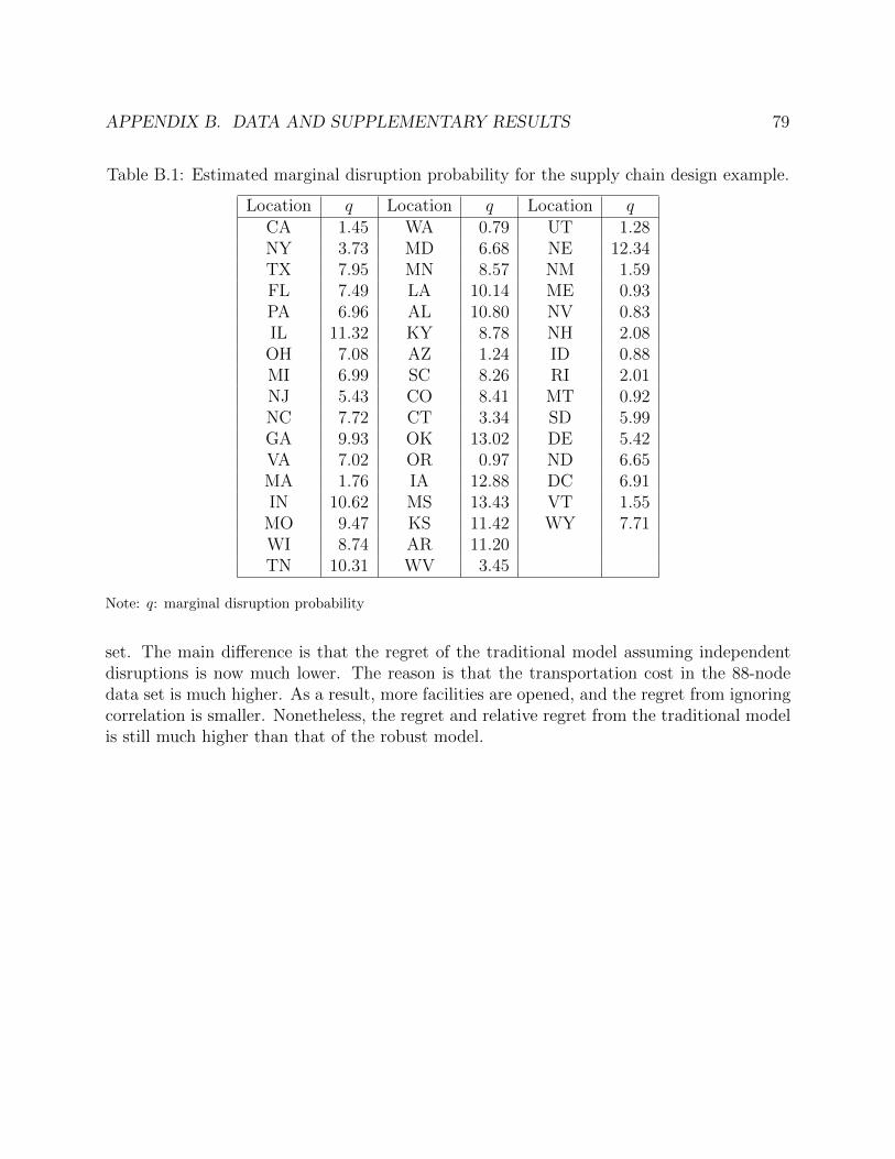
APPENDIX B. DATA AND SUPPLEMENTARY RESULTS 79

Table B.1: Estimated marginal disruption probability for the supply chain design example.

Location q Location q Location qCA 1.45 WA 0.79 UT 1.28NY 3.73 MD 6.68 NE 12.34TX 7.95 MN 8.57 NM 1.59FL 7.49 LA 10.14 ME 0.93PA 6.96 AL 10.80 NV 0.83IL 11.32 KY 8.78 NH 2.08OH 7.08 AZ 1.24 ID 0.88MI 6.99 SC 8.26 RI 2.01NJ 5.43 CO 8.41 MT 0.92NC 7.72 CT 3.34 SD 5.99GA 9.93 OK 13.02 DE 5.42VA 7.02 OR 0.97 ND 6.65MA 1.76 IA 12.88 DC 6.91IN 10.62 MS 13.43 VT 1.55

MO 9.47 KS 11.42 WY 7.71WI 8.74 AR 11.20TN 10.31 WV 3.45

Note: q: marginal disruption probability

set. The main difference is that the regret of the traditional model assuming independentdisruptions is now much lower. The reason is that the transportation cost in the 88-nodedata set is much higher. As a result, more facilities are opened, and the regret from ignoringcorrelation is smaller. Nonetheless, the regret and relative regret from the traditional modelis still much higher than that of the robust model.

APPENDIX B. DATA AND SUPPLEMENTARY RESULTS 80T

able

B.2

:Sel

ecte

dre

sult

sfo

rth

e88

-node

dat

ase

t.

αω

θnR

z R∆z R

%∆z R

CP

UR

GA

PR

nI

z I∆z I

%∆z I

CP

UI

GA

PI

0.1

20000

200

912.

130.

000.

0027

.57

0.00

912

.10

0.00

0.00

595.

280.

03

0.2

20000

200

912.

190.

000.

0019

.00

0.00

912

.13

0.00

0.00

2251

.65

0.0

60.

320

000

200

912.

240.

000.

0027

.53

0.00

912

.17

0.00

0.00

7244

.31

0.2

10.

140

000

200

912.

140.

000.

0026

.42

0.00

912

.10

0.00

0.00

602.

190.

03

0.2

40000

200

912.

190.

000.

0024

.60

0.00

912

.13

0.00

0.00

2286

.13

0.0

60.

340

000

200

912.

250.

000.

0029

.15

0.00

912

.17

0.00

0.00

7319

.25

0.2

10.

180

000

200

912.

140.

000.

0024

.86

0.00

912

.10

0.00

0.00

595.

250.

03

0.2

80000

200

912.

200.

000.

0027

.75

0.00

912

.13

0.00

0.00

2274

.91

0.0

60.

380

000

200

912.

260.

000.

0023

.51

0.00

912

.17

0.00

0.00

7318

.49

0.2

10.

120

000

400

913.

070.

000.

0018

.33

0.00

912

.23

0.00

0.00

7449

.17

0.8

10.

220

000

400

913.

590.

000.

0316

.35

0.00

912

.34

0.02

0.13

7368

.53

2.1

60.

320

000

400

914.

090.

020.

1710

.67

0.00

912

.44

0.00

0.01

7596

.53

3.4

90.

140

000

400

913.

590.

000.

0021

.15

0.00

912

.23

0.00

0.00

7581

.20

0.8

10.

240

000

400

914.

370.

000.

0314

.39

0.00

912

.34

0.02

0.13

7479

.55

2.1

60.

340

000

400

915.

100.

050.

3413

.77

0.00

912

.44

0.20

1.59

7219

.25

3.5

70.

180

000

400

914.

600.

030.

2327

.99

0.00

912

.23

0.20

1.60

7549

.96

0.8

10.

280

000

400

915.

780.

150.

9718

.97

0.00

912

.34

0.21

1.72

7428

.50

2.1

60.

380

000

400

916.

950.

291.

7014

.97

0.00

912

.44

0.20

1.59

7671

.36

3.4

90.

120

000

800

919.

930.

160.

8216

.22

0.00

912

.48

0.20

1.59

7428

.52

2.8

70.

220

000

800

923.

790.

341.

4415

.64

0.00

912

.72

0.22

1.75

7342

.71

5.3

10.

320

000

800

927.

630.

541.

9613

.44

0.00

912

.97

0.21

1.63

7313

.85

7.8

60.

140

000

800

926.

370.

562.

1316

.56

0.00

912

.48

0.20

1.59

7449

.96

2.8

70.

240

000

800

933.

440.

942.

8117

.58

0.00

912

.72

0.22

1.75

7374

.47

5.3

10.

340

000

800

940.

501.

343.

3018

.81

0.00

912

.97

0.21

1.63

7374

.53

7.8

60.

180

000

800

939.

241.

363.

4619

.35

0.00

912

.48

0.20

1.59

7414

.98

2.8

70.

280

000

800

952.

752.

144.

0517

.19

0.00

912

.72

0.22

1.75

7318

.18

5.3

10.

380

000

800

966.

252.

934.

4317

.82

0.00

912

.97

0.21

1.63

7324

.58

7.8

6

Ave

rage

921

.14

0.4

01.

9019

.98

0.00

912

.40

0.10

0.8

2608

0.49

2.54

Not

e:R

:ro

bu

stm

od

el,I:

ind

epen

den

tm

od

el,n

:nu

mb

erof

faci

liti

es,z:

exp

ecte

dco

st(×

105

),∆z:

regre

t(×

105),

%∆z:

rela

tive

regre

t

(%),

CP

U:

com

pu

tati

onti

me

(s),

GA

P:

opti

mal

ity

gap

at

term

inati

on

(%).

81

Bibliography

Aboolian, Robert, Tingting Cui, and Zuo-Jun Max Shen (2013). “An efficient approach forsolving reliable facility location models”. INFORMS Journal on Computing 25.4, pp. 720–729.

Agrawal, Shipra, Yichuan Ding, Amin Saberi, and Yinyu Ye (2010). “Correlation robuststochastic optimization”. In: Proceedings of the Twenty-First Annual ACM-SIAM Sym-posium on Discrete Algorithms. SODA ’10. Austin, Texas, pp. 1087–1096.

— (2012). “Price of correlations in stochastic optimization”. Operations Research 60.1, p-p. 150–162.

Ahmed, Shabbir, Ulas Cakmak, and Alexander Shapiro (2007). “Coherent risk measures ininventory problems”. European Journal of Operational Research 182.1, pp. 226–238.

Akcay, Alp, Bahar Biller, and Sridhar Tayur (2011). “Improved inventory targets in thepresence of limited historical demand data”. Manufacturing & Service Operations Man-agement 13.3, pp. 297–309.

An, Yu, Yu Zhang, and Bo Zeng (2011). “The reliable hub-and-spoke design problem: Modelsand algorithms”. Working paper. University of South Florida, Tampa, FL.

An, Yu, Bo Zeng, Yu Zhang, and Long Zhao (2012). “Reliable p-median facility locationproblem: Two-stage robust models and algorithms”. Working paper. University of SouthFlorida, Tampa, FL.

Arcelus, F.J., Satyendra Kumar, and G. Srinivasan (2012). “Risk tolerance and a retailer’spricing and ordering policies within a newsvendor framework”. Omega 40.2, pp. 188–198.

Aydin, Goker and Evan L. Porteus (2008). “Joint inventory and pricing decisions for anassortment”. Operations Research 56.5, pp. 1247–1255.

Barlow, Richard E., David J. Bartholomew, J. M. Bremner, and H. D. Brunk (1972). S-tatistical Inference Under Order Restrictions: The Theory and Application of IsotonicRegression. Wiley Series in Probability and Mathematical Statistics. John Wiley.

Bayarri, M. J. and James O. Berger (2004). “The interplay of Bayesian and frequentistanalysis”. Statistical Science 19.1, pp. 58–80.

Berman, Oded, Dmitry Krass, and Mozart B. C. Menezes (2007). “Facility reliability issues innetwork p-median problems: Strategic centralization and co-location effects”. OperationsResearch 55.2, pp. 332–350.

BIBLIOGRAPHY 82

Berman, Oded, Dmitry Krass, and Mozart B.C. Menezes (2013). “Location and reliabilityproblems on a line: Impact of objectives and correlated failures on optimal locationpatterns”. Omega 41.4, pp. 766–779.

Bertsimas, Dimitris, David B. Brown, and Constantine Caramanis (2011). “Theory andapplications of robust optimization”. SIAM Review 53.3, pp. 464–501.

Bertsimas, Dimitris, Karthik Natarajan, and Chung-Piaw Teo (2004). “Probabilistic com-binatorial optimization: moments, semidefinite programming, and asymptotic bounds”.SIAM Journal on Optimization 15.1, pp. 185–209.

Bertsimas, Dimitris and Aurelie Thiele (2005). A data-driven approach to newsvendor prob-lems. Tech. rep. Technical report, Massechusetts Institute of Technology.

Bertsimas, Dimitris and John N. Tsitsiklis (1997). Introduction to Linear Optimization. A-thena Scientific.

Besbes, Omar and Assaf Zeevi (2009). “Dynamic pricing without knowing the demand func-tion: Risk bounds and near-optimal algorithms”. Operations Research 57.6, pp. 1407–1420.

— (2012). “Blind network revenue management”. Operations Research 60.6, pp. 1537–1550.Best, Michael J. (1996). “An algorithm for the solution of the parametric quadratic pro-

gramming problem”. In: Applied Mathematics and Parallel Computing. Ed. by HerbertFischer, Bruno Riedaller, and Stefan Schaffler. Physica-Verlag HD, pp. 57–76.

Burnetas, Apostolos N. and Craig E. Smith (2000). “Adaptive ordering and pricing forperishable products”. Operations Research 48.3, pp. 436–443.

Chan, Lap Mui Ann, Zuo-Jun Max Shen, David Simchi-Levi, and Julie L Swann (2004).“Coordination of pricing and inventory decisions: A survey and classification”. In: Hand-book of Quantitative Supply Chain Analysis: Modeling in the e-Business Era. Ed. byDavid Simchi-Levi, S. David Wu, and Zuo-Jun Max Shen. Kluwer Academic Publishers.Chap. 9, pp. 335–392.

Chen, Fangruo and Awi Federgruen (2000). “Mean-variance analysis of basic inventory mod-els”. Technical report, Columbia University.

Chen, Qi, Xiaopeng Li, and Yanfeng Ouyang (2011). “Joint inventory-location problem underthe risk of probabilistic facility disruptions”. Transportation Research Part B: Method-ological 45.7, pp. 991–1003.

Chen, Xin and David Simchi-Levi (2012). “Pricing and inventory management”. In: TheOxford Handbook of Pricing Management. Ed. by Ozalp Ozer and Robert Phillips. OxfordUniversity Press. Chap. 30, pp. 784–822.

Chen, Youhua (Frank), Minghui Xu, and Zhe George Zhang (2009). “Technical Note – A risk-averse newsvendor model under the CVaR criterion”. Operations Research 57.4, pp. 1040–1044.

Cherkassky, Vladimir and Yunqian Ma (2004). “Practical selection of SVM parameters andnoise estimation for SVM regression”. Neural Networks 17.1, pp. 113–126.

Choi, Sungyong and Andrzej Ruszczynski (2008). “A risk-averse newsvendor with law in-variant coherent measures of risk”. Operations Research Letters 36.1, pp. 77–82.

BIBLIOGRAPHY 83

Choi, Sungyong, Andrzej Ruszczynski, and Yao Zhao (2011). “A multiproduct risk-aversenewsvendor with law-invariant coherent measures of risk”. Operations Research 59.2,pp. 346–364.

Chu, Leon Yang, J. George Shanthikumar, and Zuo-Jun Max Shen (2008). “Solving oper-ational statistics via a Bayesian analysis”. Operations Research Letters 36.1, pp. 110–116.

— (2009). “Pricing and revenue management with operational statistics”. Working paper,University of California, Berkeley.

Church, Richard L. and Maria P. Scaparra (2007). “Protecting critical assets: The r-interdictionmedian problem with fortification”. Geographical Analysis 39.2, pp. 129–146.

Church, Richard L., Maria P. Scaparra, and Richard S. Middleton (2004). “Identifying criticalinfrastructure: The median and covering facility interdiction problems”. Annals of theAssociation of American Geographers 94.3, pp. 491–502.

Cryer, Jonathan D., Tim Robertson, F. T. Wright, and Robert J. Casady (1972). “Monotonemedian regression”. The Annals of Mathematical Statistics 43.5, pp. 1459–1469.

Cui, Tingting, Yanfeng Ouyang, and Zuo-Jun Max Shen (2010). “Reliable facility locationdesign under the risk of disruptions”. Operations Research 58.4, pp. 998–1011.

Daskin, Mark S. (1995). Network and Discrete Location. John Wiley & Sons, Inc.Edmonds, Jack (1971). “Matroids and the greedy algorithm”. Mathematical Programming

1.1, pp. 127–136.Eeckhoudt, Louis, Christian Gollier, and Harris Schlesinger (1995). “The risk-averse (and

prudent) newsboy”. Management Science 41.5, pp. 786–794.Elmaghraby, Wedad and Pınar Keskinocak (2003). “Dynamic pricing in the presence of

inventory considerations: Research overview, current practices, and future directions”.Management Science 49.10, pp. 1287–1309.

Federgruen, Awi and Aliza Heching (1999). “Combined pricing and inventory control underuncertainty”. Operations Research 47.3, pp. 454–475.

Feng, Qi, Sirong Luo, and Dan Zhang (2014). “Dynamic inventory-pricing control underbackorder: Demand estimation and policy optimization”. Manufacturing & Service Op-erations Management 16.1, pp. 149–160.

Gallego, Guillermo and Ilkyeong Moon (1993). “The distribution free newsboy problem:Review and extensions”. The Journal of the Operational Research Society 44.8, pp. 825–834.

Gallego, Guillermo and Garrett van Ryzin (1994). “Optimal dynamic pricing of inventorieswith stochastic demand over finite horizons”. Management Science 40.8, pp. 999–1020.

Gotoh, Jun-Ya and Yuichi Takano (2007). “Newsvendor solutions via conditional value-at-risk minimization”. European Journal of Operational Research 179.1, pp. 80–96.

Hayes, Robert H. (1969). “Statistical estimation problems in inventory control”. ManagementScience 15.11, pp. 686–701.

Huh, Woonghee Tim and Paat Rusmevichientong (2009). “A nonparametric asymptotic anal-ysis of inventory planning with censored demand”. Mathematics of Operations Research34.1, pp. 103–123.

BIBLIOGRAPHY 84

Huh, Woonghee Tim, Retsef Levi, Paat Rusmevichientong, and James B. Orlin (2011).“Adaptive data-driven inventory control with censored demand based on Kaplan-Meierestimator”. Operations Research 59.4, pp. 929–941.

Ibragimov, I. A. and R. Z. Has’Minskii (1981). Statistical Estimation: Asymptotic Theory.Springer-Verlag, New York.

Iglehart, Donald L. (1964). “The dynamic inventory problem with unknown demand distri-bution”. Management Science 10.3, pp. 429–440.

Jain, Ankit, Andrew E. B. Lim, J. George Shanthikumar, and Lian Yu (2011). “Objectiveoperational learning with application to newsvendor problem”. Working paper. Universityof California, Berkeley.

Karlin, Samuel and Charles R. Carr (1962). “Prices and optimal inventory policy”. In: Studiesin Applied Probability and Management Science. Ed. by Kenneth Arrow, Samuel Karlin,and Herbert Scarf. Stanford University Press, Stanford, CA, pp. 159–172.

Kocabıyıkoglu, Ayse and Ioana Popescu (2011). “An elasticity approach to the newsvendorwith price-sensitive demand”. Operations Research 59.2, pp. 301–312.

Koenker, Roger and Gilbert Bassett Jr. (1978). “Regression quantiles”. Econometrica 46.1,pp. 33–50.

Koenker, Roger, Pin Ng, and Stephen Portnoy (1994). “Quantile smoothing splines”. Biometri-ka 81.4, pp. 673–680.

Levi, Retsef, Gerogia Perakis, and Joline Uichanco (2012). “The data-driven newsvendorproblem: New bounds and insights”. Working paper, Massachusetts Institute of Technol-ogy.

Levi, Retsef, Robin O. Roundy, and David B. Shmoys (2007). “Provably near-optimalsampling-based policies for stochastic inventory control models”. Mathematics of Op-erations Research 32.4, pp. 821–839.

Li, Qingwei, Bo Zeng, and Alex Savachkin (2013). “Reliable facility location design underdisruptions”. Computers & Operations Research 40.4, pp. 901–909.

Li, Xiaopeng and Yanfeng Ouyang (2010). “A continuum approximation approach to reli-able facility location design under correlated probabilistic disruptions”. TransportationResearch Part B: Methodological 44.4, pp. 535–548.

— (2011). “Reliable sensor deployment for network traffic surveillance”. Transportation Re-search Part B: Methodological 45.1, pp. 218–231.

— (2012). “Reliable traffic sensor deployment under probabilistic disruptions and general-ized surveillance effectiveness measures”. Operations Research 60.5, pp. 1183–1198.

Li, Xiaopeng, Yanfeng Ouyang, and Fan Peng (2013). “A supporting station model forreliable infrastructure location design under interdependent disruptions”. TransportationResearch Part E: Logistics and Transportation Review. Forthcoming.

Liang, Yong, Zuo-Jun Max Shen, and Ye Xu (2013). “Flexible hub location model for airtransportation networks”. Working paper. University of California, Berkeley, CA.

Liberatore, Federico, Maria P. Scaparra, and Mark S. Daskin (2012). “Hedging against dis-ruptions with ripple effects in location analysis”. Omega 40.1, pp. 21–30.

BIBLIOGRAPHY 85

Lim, Andrew E. B., J. George Shanthikumar, and Zuo-Jun Max Shen (2006). “Model uncer-tainty, robust optimization, and learning”. In: TutORials in Operations Research: Models,Methods, and Applications for Innovative Decision Making. INFORMS. Chap. 3, pp. 66–94.

Lim, Michael K., Mark S. Daskin, Achal Bassamboo, and Sunil Chopra (2010). “A facilityreliability problem: Formulation, properties, and algorithm”. Naval Research Logistics57.1, pp. 58–70.

Lim, Michael K., Achal Bassamboo, Sunil Chopra, and Mark S. Daskin (2013). “Facilitylocation decisions with random disruptions and imperfect estimation”. Manufacturing &Service Operations Management 15.2, pp. 239–249.

Liyanage, Liwan H. and J. George Shanthikumar (2005). “A practical inventory controlpolicy using operational statistics”. Operations Research Letters 33.4, pp. 341 –348.

Losada, Chaya, M.Paola Scaparra, RichardL. Church, and MarkS. Daskin (2012). “The s-tochastic interdiction median problem with disruption intensity levels”. Annals of Oper-ations Research 201.1, pp. 345–365.

Lu, Ye and David Simchi-Levi (2013). “On the unimodality of the profit function of thepricing newsvendor”. Production and Operations Management 22.3, pp. 615–625.

Magnanti, Thomas L. and Richard T. Wong (1981). “Accelerating Benders decomposition:Algorithmic enhancement and model selection criteria”. Operations Research 29.3, p-p. 464–484.

Mak, Ho-Yin and Zuo-Jun Max Shen (2012). “Risk diversification and risk pooling in supplychain design”. IIE Transactions 44.8, pp. 603–621.

Mills, Edwin S. (1959). “Uncertainty and price theory”. The Quarterly Journal of Economics73.1, pp. 116–130.

Murray, Chase C., Abhijit Gosavi, and Debabrata Talukdar (2012). “The multi-productprice-setting newsvendor with resource capacity constraints”. International Journal ofProduction Economics 138.1, pp. 148–158.

Peng, Peng, Lawrence V. Snyder, Andrew Lim, and Zuli Liu (2011). “Reliable logistics net-works design with facility disruptions”. Transportation Research Part B: Methodological45.8, pp. 1190–1211.

Perakis, Georgia and Guillaume Roels (2008). “Regret in the newsvendor model with partialinformation”. Operations Research 56.1, pp. 188–203.

Petruzzi, N. C. and M. Dada (1999). “Pricing and the newsvendor problem: A review withextensions”. Operations Research 47.2, pp. 183–194.

Portnoy, Stephen (1991). “Asymptotic behavior of the number of regression quantile break-points”. SIAM Journal on Scientific and Statistical Computing 12.4, pp. 867–883.

Potschka, Andreas, Christian Kirches, Hans Georg Bock, and Johannes P Schloder (2010).“Reliable solution of convex quadratic programs with parametric active set methods”.Technical Report, Heidelberg University.

Qi, Lian and Zuo-Jun Max Shen (2007). “A supply chain design model with unreliablesupply”. Naval Research Logistics 54.8, pp. 829–844.

BIBLIOGRAPHY 86

Qi, Lian, Zuo-Jun Max Shen, and Lawrence V. Snyder (2010). “The effect of supply disrup-tions on supply chain design decisions”. Transportation Science 44.2, pp. 274–289.

Ramamurthy, Vivek, J. George Shanthikumar, and Zuo-Jun Max Shen (2012). “Inventorypolicy with parametric demand: Operational statistics, linear correction, and regression”.Production and Operations Management 21.2, pp. 291–308.

Raz, Gal and Evan L. Porteus (2006). “A fractiles perspective to the joint price/quantitynewsvendor model”. Management Science 52.11, pp. 1764–1777.

Rockafellar, R. Tyrrell and Stanislav Uryasev (2000). “Optimization of conditional value-at-risk”. Journal of Risk 2.3, pp. 21–42.

Roels, Guillaume (2013). “Risk premiums in the price-setting newsvendor model”. W3orkingpaper, University of California, Los Angeles.

Salinger, Michael and Miguel Ampudia (2011). “Simple economics of the price-setting newsven-dor problem”. Management Science 57.11, pp. 1996–1998.

Scaparra, Maria P. and Richard L. Church (2008a). “A bilevel mixed-integer program forcritical infrastructure protection planning”. Computers & Operations Research 35.6, p-p. 1905–1923.

— (2008b). “An exact solution approach for the interdiction median problem with fortifica-tion”. European Journal of Operational Research 189.1, pp. 76–92.

Scarf, Herbert (1958). “A min-max solution of an inventory problem”. In: Studies in TheMathematical Theory of Inventory and Production. Ed. by Kenneth J. Arrow, SamuelKarlin, and Herbert Scarf. Stanford University Press. Chap. 12, pp. 201–209.

— (1959). “Bayes solutions of the statistical inventory problem”. The Annals of Mathemat-ical Statistics 30.2, pp. 490–508.

Schwarz, Gideon (1978). “Estimating the dimension of a model”. The Annals of Statistics6.2, pp. 461–464.

Shen, Zuo-Jun Max, Roger Lezhou Zhan, and Jiawei Zhang (2011). “The reliable facilitylocation problem: Formulations, heuristics, and approximation algorithms”. INFORMSJournal on Computing 23.3, pp. 470–482.

Snyder, Lawrence V. and Mark S. Daskin (2005). “Reliability models for facility location:The expected failure cost case”. Transportation Science 39.3, pp. 400–416.

— (2006). “Stochastic p-robust location problems”. IIE Transactions 38.11, pp. 971–985.Snyder, Lawrence V., Zumbul Atan, Peng Peng, Ying Rong, Amanda J. Schmitt, and Burcu

Sinsoysal (2012). “OR/MS models for supply chain disruptions: A review”. Workingpaper. Lehigh University, Bethlehem, PA.

Suykens, Johan A.K. and Joos Vandewalle (1999). “Least squares support vector machineclassifiers”. Neural Processing Letters 9.3, pp. 293–300.

Takeuchi, Ichiro, Quoc V. Le, Timothy D. Sears, and Alexander J. Smola (2006). “Nonpara-metric quantile estimation”. Journal of Machine Learning Research 7, pp. 1231–1264.

Tang, Christopher S. (2006). “Perspectives in supply chain risk management”. InternationalJournal of Production Economics 103.2, pp. 451–488.

Wahba, Grace (1999). “Support vector machines, reproducing kernel Hilbert spaces and therandomized GACV”. In: Advances in Kernel Methods-Support Vector Learning. Ed. by

BIBLIOGRAPHY 87

Bernhard Scholkopf, Christopher J. C. Burges, and Alexander J. Smola. MIT Press.Chap. 6, pp. 69–87.

Wang, Zizhuo, Shiming Deng, and Yinyu Ye (2011). “Close the gaps: A learning-while-doingalgorithm for a class of single-product revenue management problems”. Working paper.Stanford University.

Wang, Zizhuo, Peter W. Glynn, and Yinyu Ye (2010). “Likelihood robust optimization fordata-driven newsvendor problems”. Working paper, Stanford University.

Whitin, Thomas M. (1955). “Inventory control and price theory”. Management Science 2.1,pp. 61–68.

Xu, Minghui, Youhua (Frank) Chen, and Xiaolin Xu (2010). “The effect of demand uncer-tainty in a price-setting newsvendor model”. European Journal of Operational Research207.2, pp. 946 –957.

Xu, Minghui and Ye Lu (2013). “The effect of supply uncertainty in price-setting newsvendormodels”. European Journal of Operational Research 227.3, pp. 423–433.

Xu, Xiaolin, Xiaoqiang Cai, and Youhua (Frank) Chen (2011). “Unimodality of price-settingnewsvendor’s objective function with multiplicative demand and its applications”. Inter-national Journal of Production Economics 133.2, pp. 653 –661.

Yang, Lei, Minghui Xu, Gang Yu, and Hanqin Zhang (2009). “Supply chain coordinationwith CVaR criterion”. Asia-Pacific Journal of Operational Research 26.01, pp. 135–160.

Yang, Shilei, Chunming Victor Shi, and Xuan Zhao (2011). “Optimal ordering and pricingdecisions for a target oriented newsvendor”. Omega 39.1, pp. 110–115.

Yano, Candace A. and Stephen M. Gilbert (2004). “Coordinated pricing and production/procurement decisions: A review”. In: Managing Business Interfaces. Ed. by Amiya K.Chakravarty and Jehoshua Eliashberg. Vol. 16. International Series in Quantitative Mar-keting. Springer US, pp. 65–103.

Yao, Li, Youhua (Frank) Chen, and Houmin Yan (2006). “The newsvendor problem with pric-ing: Extensions”. International Journal of Management Science and Engineering Man-agement 1.1, pp. 3–16.

Young, Leslie (1978). “Price, inventory and the structure of uncertain demand”. New ZealandOperations Research 6.2, pp. 157–177.

essays on supply chain management with model uncertainty

Documents