essays on the economics of education and...
TRANSCRIPT

THE LONDON SCHOOL OF ECONOMICS AND POLITICAL SCIENCE
ESSAYS ON THE ECONOMICS OFEDUCATION AND FERTILITY
Tiloka de Silva
thesis submitted to the Department of Economicsof the London School of Economics
for the degree of doctor of philosophyJuly 2017

Declaration
I certify that the thesis I have presented for examination for the MPhil/PhD
degree of the London School of Economics and Political Science is solely my
own work other than where I have clearly indicated that it is the work of others
(in which case the extent of any work carried out jointly by me and any other
person is clearly identified in it).
The copyright of this thesis rests with the author. Quotation from it is per-
mitted, provided that full acknowledgement is made. This thesis may not be
reproduced without my prior written consent.
I warrant that this authorisation does not, to the best of my belief, infringe
the rights of any third party. I declare that my thesis consists of 36,888 words.
2

Statement of inclusion of previous work
I confirm that Chapter 2 is a heavily revised version of the paper I submitted
at the end of my MRes in 2014.
Statement of conjoint work
I confirm that Chapters 2 and 3 were jointly co-authored with Professor Silvana
Tenreyro of LSE and I contributed 50% of this work.
3

Acknowledgements
The work contained in this thesis has benefited from the help and support of
many people. I am immensely grateful to my supervisor, Silvana Tenreyro, for
her invaluable guidance, advice and patience throughout my time at the LSE
and for teaching me not to lose sight of the bigger picture. I would also like
to thank her in her capacity as a co-author of the second and third chapters
of this thesis.
I am extremely grateful to Steve Pischke and Guy Michaels for taking the
time to give me comments, feedback and support. I would also like to thank
Francesco Caselli, Per Krusell and all the members of the LSE Macroeconomics
seminar.
My friends have been a great source of strength, especially Laura, Shan, Chao,
Shashini, Saki, and Sha, who have been sounding boards, cheerleaders and
companions all rolled into one over the past five years.
Finally, I would not have been able to write this thesis without the love and
support of my family. My parents and brother never let me doubt that I
could do it, even when I was convinced otherwise. My deepest gratitude is to
Tharindu, whose ability to always make me laugh has been invaluable over the
past five years.
4

Contents
Declaration 2
Conjoint work 3
Acknowledgements 4
List of Tables 7
List of Figures 8
1 Introduction 9
2 The Rat Race for Human Capital: Evidence and Theory 12
2.1 Introduction . . . . . . . . . . . . . . . . . . . . . . . . . . . . . 12
2.2 Related literature . . . . . . . . . . . . . . . . . . . . . . . . . . 16
2.3 The Korean context . . . . . . . . . . . . . . . . . . . . . . . . . 20
2.4 Data . . . . . . . . . . . . . . . . . . . . . . . . . . . . . . . . . 25
2.5 Empirical strategy . . . . . . . . . . . . . . . . . . . . . . . . . 31
2.6 Effect of the curfew . . . . . . . . . . . . . . . . . . . . . . . . . 34
2.7 Results . . . . . . . . . . . . . . . . . . . . . . . . . . . . . . . . 39
2.8 Robustness checks . . . . . . . . . . . . . . . . . . . . . . . . . . 47
2.9 Theoretical framework . . . . . . . . . . . . . . . . . . . . . . . 57
2.10 Conclusion . . . . . . . . . . . . . . . . . . . . . . . . . . . . . . 66
Appendix . . . . . . . . . . . . . . . . . . . . . . . . . . . . . . . . . 68
3 Population Control Policies and Fertility Convergence 75
3.1 Introduction . . . . . . . . . . . . . . . . . . . . . . . . . . . . . 75
3.2 Fertility patterns across time and space . . . . . . . . . . . . . . 77
5

3.3 The global family planning movement and its consequences . . . 80
3.4 Considering other explanations for the decline in fertility . . . . 95
3.5 Conclusion . . . . . . . . . . . . . . . . . . . . . . . . . . . . . . 102
Appendix . . . . . . . . . . . . . . . . . . . . . . . . . . . . . . . . . 104
4 The Large Fall in Global Fertility: A Quantitative Model 129
4.1 Introduction . . . . . . . . . . . . . . . . . . . . . . . . . . . . . 129
4.2 The Model . . . . . . . . . . . . . . . . . . . . . . . . . . . . . . 131
4.3 Calibration . . . . . . . . . . . . . . . . . . . . . . . . . . . . . 137
4.4 Results . . . . . . . . . . . . . . . . . . . . . . . . . . . . . . . . 143
4.5 Extensions and robustness checks . . . . . . . . . . . . . . . . . 146
4.6 Conclusion . . . . . . . . . . . . . . . . . . . . . . . . . . . . . . 157
Appendix . . . . . . . . . . . . . . . . . . . . . . . . . . . . . . . . . 158
Bibliography 159
6
List of Tables
2.1 Curfew imposed on Hagwon operating hours for high schoolstudents . . . . . . . . . . . . . . . . . . . . . . . . . . . . . . . 24
2.2 Descriptive statistics . . . . . . . . . . . . . . . . . . . . . . . . 272.3 Determinants of private tutoring expenditure . . . . . . . . . . . 302.4 Effect of the curfew on spending on tutoring . . . . . . . . . . . 362.5 Effect of tutoring expenditure on college entrance . . . . . . . . 412.6 Effect of tutoring expenditure on college entrance . . . . . . . . 422.7 Results of two-sample 2SLS estimation . . . . . . . . . . . . . . 452.8 Effect of curfew on tutoring by type . . . . . . . . . . . . . . . . 492.9 Measurement error in tutoring expenditure . . . . . . . . . . . . 552.10 Transition matrix for internal migration for 20-24 year olds . . . 57
3.1 Number of countries with government goals for fertility policy . 823.2 Number of countries by government support for family planning 823.3 Change in total fertility rates (TFRs) and funding for family
planning programmes . . . . . . . . . . . . . . . . . . . . . . . 913.4 Change in total fertility rates (TFRs) and family planning pro-
gramme effort . . . . . . . . . . . . . . . . . . . . . . . . . . . 933.5 Change in total fertility rates (TFRs) and exposure to family
planning messages . . . . . . . . . . . . . . . . . . . . . . . . . 943.6 Fertility change by education in 2010 . . . . . . . . . . . . . . . 993.7 Changes in wanted and unwanted fertility (as a percentage of
change in total fertility rate) . . . . . . . . . . . . . . . . . . . . 101
4.1 Calibration of structural parameters . . . . . . . . . . . . . . . . 1414.2 Estimation of ϕ and φ . . . . . . . . . . . . . . . . . . . . . . . 1434.3 Estimation of ϕ and φ with mortality . . . . . . . . . . . . . . . 149
7

List of Figures
2.1 Trends in no. of students enrolled in and no. of tertiary educa-tion institutions . . . . . . . . . . . . . . . . . . . . . . . . . . . 21
2.2 Effect of the curfew by years of exposure and parental education 382.3 Effect of the curfew on time use . . . . . . . . . . . . . . . . . . 52
3.1 Fertility histograms over time . . . . . . . . . . . . . . . . . . . 773.2 Fertility trends across regions . . . . . . . . . . . . . . . . . . . 783.3 Fertility – income relation in 1960 and 2013 . . . . . . . . . . . 793.4 Evolution of fertility rates by policy in 1976 . . . . . . . . . . . 903.5 Fertility and urbanisation . . . . . . . . . . . . . . . . . . . . . 97
4.1 Transition to steady state . . . . . . . . . . . . . . . . . . . . . 1444.2 Incorporating mortality . . . . . . . . . . . . . . . . . . . . . . . 1504.3 Number of surviving children . . . . . . . . . . . . . . . . . . . 1514.4 Incorporating unwanted fertility . . . . . . . . . . . . . . . . . . 1544.5 Comparing functional forms . . . . . . . . . . . . . . . . . . . . 156
8

Chapter 1
Introduction
This thesis studies two topics in the macro-labour literature: investment in
human capital and fertility decisions. The thesis comprises of three chapters,
the first studying the effects of private tutoring in Korea and its resemblance
to a human capital rat race and the second and third investigating the rapid
decline in fertility rates experienced in developing countries over the past few
decades.
With many countries having reached universal primary and secondary educa-
tion, parental spending on education for supplementary and enrichment pur-
poses has begun to resemble a rat race. In many Asian countries, it is normal
for students to receive some or several forms of private tutoring alongside for-
mal schooling. However, unlike the returns to schooling or the effects of school
quality on student achievement which have been widely studied, the effects
of private tutoring have received limited attention. In the first substantive
chapter of this thesis, I exploit exogenous variation in spending on private
tutoring caused by the imposition of a curfew on the operating hours of tu-
toring institutes in Korea, to estimate the impact of spending on tutoring on
long-term educational and labour market outcomes. The first stage estimates
highlight the severity of the rat race, with curfews imposed as late as 10pm
still constraining tutoring expenditure. While I do not find any significant
9
effects of tutoring expenditure on entering college, when I interact tutoring
expenditure with parental education, I find a significant, positive effect of tu-
toring on attending any college for children of less educated parents, while the
effect for children of more educated parents is not significantly different from
zero. Given that the less educated parents spend much less on tutoring, these
results indicate diminishing marginal effects of tutoring, while the lack of an
effect in the specification linear in tutoring expenditure points to the average
impact (local to those constrained by the curfew) being close to zero. I also
find that tutoring expenditure has a positive effect on both completing a four
year degree and on being employed. I place these empirical findings within an
asymmetric information framework to explain how the use of test scores as a
signal for ability leads to inefficiently high investments in tutoring, leading to
a rat-race equilibrium.
The second paper highlights the trends in fertility rates observed in develop-
ing countries, pointing out that cross-country differences in fertility rates have
fallen very rapidly over the past four decades, with most countries converging
to a rate just above two children per woman. In the second substantive chapter
in the thesis, my co-author and I argue that the convergence in fertility rates
has taken place despite the limited (or absent) absolute convergence in other
economic variables and propose an alternative explanation for the decline in
fertility rates: the population-control programmes started in the 1960s which
aimed to increase information about and availability of contraceptive methods,
and establish a new small-family norm using public campaigns. Using several
different measures of family planning programme intensity across countries,
we show a strong positive association between programme intensity and sub-
sequent reductions in fertility, after controlling for other potential explanatory
variables, such as GDP, schooling, urbanisation, and mortality rates. We con-
clude that concerted population control policies implemented in developing
countries are likely to have played a central role in accelerating the global de-
cline in fertility rates and can explain some patterns of that fertility decline
that are not well accounted for by other socioeconomic factors.
10

In the third main chapter of the thesis, we build on the findings presented in
the previous chapter by studying a quantitative model of endogenous human
capital and fertility choice, augmented to portray a role for social norms over
the number of children. The model allows us to gauge the role of human capital
accumulation on the decline in fertility and to simulate the implementation of
population-control policies aimed at affecting social norms on family size. We
also consider extensions of the model in which we allow a role for the decline in
infant and child mortality and for improvements in contraceptive technologies
(the second main component of the population-control programmes). Using
data on several socio-economic variables as well as information on funding for
family planning programmes to parametrise the model, we find that, as argued
in the previous chapter, policies aimed at altering family-size norms provided
a significant impulse to accelerate and strengthen the decline in fertility that
would have otherwise gradually taken place as economies move to higher levels
of human capital and lower levels of mortality.
11

Chapter 2
The Rat Race for Human
Capital: Evidence and Theory
2.1 Introduction
Educational attainment has shown tremendous improvements in most parts of
the world over the past few decades, building up the stock of human capital
and spurring economic growth. However, as more and more countries pass the
milestones of universal primary and secondary education, the acquisition of ed-
ucation is beginning to resemble what Akerlof (1976) described as a “rat race”,
with parents spending increasing amounts to ensure that their children attend
the best schools and universities. In some countries this type of behaviour is
limited to households belonging to the higher income brackets, but in many
countries, particularly those in Asia, it is much more widespread. According
to the OECD Programme for International Student Assessment (PISA) re-
sults from 2009, 43 percent of 15 year old students surveyed from 65 countries
participated in mathematics classes after school. However, this average masks
wide variation between countries and regions. For instance, more than 75 per-
cent of students in Japan or Korea take supplementary classes, whereas only
around 15 percent in Sweden or Finland do so (OECD 2010). Interestingly,
12

the correlation between a country’s per capita GDP and the percentage of stu-
dents engaging in supplementary maths classes in the country is negative but
there is substantial variation within income groups. Even in the group of high
income countries (as classified by the World Bank), 62 percent of students in
Asian countries attend private tutoring, whereas in Europe and North America
the participation rates are 33 and 20 percent, respectively.
While the returns to years of schooling and effects of school quality on student
achievement have been widely studied, the effects of spending on supplemen-
tary education including private tutoring have received limited attention.1 The
identification of these effects is challenging as these expenditures are likely to
be related to many unobserved factors such as parental ambitions for their
children or the motivation and ability of the child. Within the literature that
investigates the effects of private tutoring, many papers ignore the endogene-
ity of the private tutoring decision, while the papers that do not, study the
effects of tutoring on test scores or self-assessed academic ability. In this pa-
per, I exploit exogenous variation in spending on private tutoring caused by
the imposition of a curfew on Hagwon (private institutes operating outside of
formal schooling offering private tutoring) in South Korea, to obtain causal
estimates of the effects of expenditure on tutoring on longer-term outcomes
such as college entrance and completion, and employment.
Korea consistently ranks very highly on international standardised tests such as
the PISA tests administered by the OECD. At the same time, the importance
placed on test scores for college admissions and the intense competition to
enter prestigious universities have resulted in Korea having the highest rate
of participation in private tutoring in the world. In 2015, 68.8 percent of all
students attended after-school or weekend classes and expenditure on tutoring
accounted for 5.5 percent of average household spending (KOSIS 2017a, 2017c).
1The type of spending depends on the nature of the competition - education systemscharacterised by high-stakes entrance examinations for secondary schools or universities areaccompanied by high levels of participation in private tutoring whereas in systems placingmore emphasis on individuality parents may spend more on extra-curricular activities. Inthis paper, I will be focusing on private tutoring obtained at a fee.
13

Over the past few decades the state has made several attempts to regulate the
private tutoring sector, one of the more recent being the curfew on operating
hours of Hagwon.
In this paper, I use data from the Korean Youth Panel (YP) which follows
around 10,000 individuals aged between 15 and 29 for eight years starting in
2007. For a sub-sample of 2,710 individuals (belonging to five high-school
graduation cohorts) who are still attending high school during the survey pe-
riod, I observe data on monthly spending on tutoring in their final year of high
school as well as what they do after leaving school, in particular, whether they
go to college or not. An individual’s exposure to the curfew is determined
by the region in which they attend school as well as the year in which they
graduate from high school. After controlling for region and year fixed effects,
exposure to the curfew is plausibly exogenous and is used as an instrument in
the analysis. To estimate the impact on longer term outcomes such as degree
completion and employment, I combine the Youth Panel data on private tu-
toring expenditure with data from a sub-sample of 18,908 individuals from the
2016 Regional Labour Force Survey (LFS) to conduct a two-sample two stage
least squares (TS2SLS) estimation.
I first explore the effect of the curfew which was imposed at either 10pm
or 11pm in seven of the sixteen provinces in Korea. I find that the 10pm
curfew significantly reduced spending on tutoring. Using time use data for high
school students, I also find that the 10pm curfew led to significant increases
in sleeping hours, confirming my first stage estimates. The very fact that a
curfew was imposed to control excessive spending on tutoring together with
the fact that students appear to be trading off sleep for additional tutoring
provide an indication of the severity of the college entrance rat race in Korea.
The estimated effects of tutoring expenditure on educational and labour mar-
ket outcomes vary significantly depending on the outcome considered. Es-
timates from a regression model which is linear in tutoring expenditure do
not show any significant effects on college entrance. However, when I interact
14

tutoring expenditure with parental education, I find a significant, positive ef-
fect of tutoring on attending any college for children of less educated parents,
though the effect for children of more educated parents is still not significantly
different from zero. Given that the more educated parents spend significantly
more on tutoring for their children, these results indicate diminishing marginal
effects of tutoring, while the lack of an effect in the model linear in tutor-
ing expenditure points to the average effect being close to zero. Given that
two-stage least squares (2SLS) captures the Local Average Treatment Effect
(LATE), which, in this case, is the effect on those whose spending was high
enough to be constrained by the curfew, this result is not surprising. With
regards to the longer-term outcomes, the two-sample 2SLS results show that
tutoring expenditure has positive effects on both college completion and on
being employed.
While my identification of the effects of tutoring does not allow me to dis-
tinguish between signalling and human capital explanations for the choice of
tutoring, the Korean college admissions system which relies heavily on test
scores, the imposition of a curfew to curb private tutoring, and my results
from the first stage are strongly indicative of a rat race. Therefore, I explain
my findings within a simple, asymmetric information framework where stu-
dents signal ability using test scores, which then determines college entrance.
Test scores are a function of innate ability, tutoring, and formal schooling,
with high ability students having a comparative advantage in transforming
tutoring into test scores. Under these conditions, a separating equilibrium
emerges in which the high types spend more on tutoring than they would
under perfect information, leading to an inefficient level of expenditure - a
rat-race equilibrium. I then show how a higher college premium and, under
certain conditions, improvements in school quality, could further drive up the
spending of the high types, leading them to experience lower and lower returns
to spending on tutoring.
The remainder of the paper is organised as follows. In the following section,
15

I discuss the contribution of this paper in relation to the literature - both
empirical and theoretical. In Section 2.3, I provide some background into the
private tutoring sector in Korea and briefly discuss attempts by the state to
regulate the sector. I describe the data in Section 2.4 and discuss the estimation
strategy in Section 2.5. Section 2.6 presents the first stage estimates while
Section 2.7 presents the estimated effects of spending on tutoring on college
entrance as well as longer term outcomes. Section 2.8 presents some robustness
checks and Section 2.9 lays out the theoretical model used to reconcile the
findings with economic theory. Section 2.10 concludes.
2.2 Related literature
In this section, I discuss the contribution of this paper in relation to the em-
pirical and theoretical literature on the subject. While there are many papers
that discuss the impact of tutoring with no attempt to account for the en-
dogeneity of the choice of tutoring, I focus here on those papers that make
explicit efforts to address this issue.
2.2.1 Empirical work
Unlike the returns to schooling and effects of educational inputs such as school
quality on academic achievement on which there exists a rich literature, the
body of work on the impact of tutoring is much smaller, with no consensus
on the effectiveness of tutoring. Several studies investigating the effect of
private tutoring on academic achievement find positive associations between
tutoring and test scores but most of these papers either ignore or do not
convincingly address the endogeneity of private tutoring (for a review of this
work, see Bray and Lykins 2012). Given that spending on private tutoring
is strongly affected by family, school and individual characteristics, many of
which are unobserved, the bias in estimates that treat the consumption of
16

private tutoring as exogenous could be large. Therefore, in this section, I
focus on studies that make explicit efforts to address the issue of endogeneity.
A few papers examine the impact of remedial programmes targeted at low-
performing students under experimental or quasi-experimental settings. Ban-
nerjee, Cole, Duflo and Linden (2007) analyse the effects of a randomised
experiment in India in which remedial classes were provided to primary school
students lagging behind in basic numeracy and literacy skills and find that
the programme had significant effects on the students’ test scores. Lavy and
Schlosser (2005) evaluate the effects of a remedial programme for underper-
forming high school students in Israel using a differences-in-differences strat-
egy and find that the programme improved enrollment rates while Jacob and
Lefgren (2004) find positive effects of summer school programmes on the test
scores of low-performing primary and middle school students using a regression
discontinuity design. A key difference between these papers and this paper is
their focus on targeted remedial programmes which are provided free of charge
for low-performing students. In contrast, this paper focuses on the effects of
spending on tutoring, which is chosen at the discretion of the student or par-
ents and is not restricted to low-performing students. Another difference is
that students in Korea already spend more than 30 hours a week in formal
schooling, more than in any of the countries analysed in these papers.2
The decision on spending on private tutoring depends on many factors - aside
from the characteristics of the child, the aspirations of the parents for that
child as well as the financial circumstances of the family matter. As such,
isolating a source of exogenous variation in spending on tutoring is challeng-
ing. Papers which make an attempt to identify such variation include work
by Suryadarma, Suryahadi, Sumarto and Rogers (2006), Dang (2007), Kang
(2007), Ryu and Kang (2013), and Zhang (2013). These studies are carried
out in East Asian countries in which private tutoring is highly prevalent and
2The PISA results for 2015 show that 15 year olds in Korea spend more than 30 hoursper week on average in regular lessons; 3 hours more than the OECD average, 2.5 hoursmore than the US average and 2 hours more than the Israeli average (OECD 2016b).
17

identify the impact of tutoring on academic achievements using instrumental
variable (IV) methods.
Dang (2007) follows a strategy similar to that used in this paper and uses the
state-regulated, average price of tutoring charged by schools in the commune
as an instrument for hours spent on private tutoring for elementary and middle
school students in Vietnam. The author finds that tutoring leads to a signifi-
cant improvement in a self-reported measure of academic ranking, with larger
effects for lower secondary school students.
Other papers in the literature use individual level instruments for identifica-
tion. Suryadarma et al. (2006) use the proportion of peers participating in
tutoring as an instrument for participation in tutoring among primary school
students in Indonesia while Zhang (2013) employs both peer participation in
tutoring and proximity of the student’s home to private tutoring centres as
instruments for participation in tutoring among high school students in the Ji-
nan province in China. Kang (2007) and Ryu and Kang (2013) consider birth
order as an instrument for spending on private tutoring among high school and
middle school students in Korea. These papers find that the effect of tutoring
on academic achievement is modest at best.
Using peer participation as an instrument could be problematic in the event
of spillover effects or if peer groups are formed on the basis of participation
in tutoring while birth order could possibly influence other types of parental
investments which also affect academic achievement. These studies also focus
on test scores as the measure of academic achievement (Suryadarma et al.
(2006) and Ryu and Kang (2013) use scores from tests administered as part of
the survey from which data is collected, while Zhang (2013) and Kang (2007)
consider university entrance examination scores) and do not find much of an
effect of tutoring.
The key contribution of this paper is the focus on outcomes such as college
entrance and completion, and employment, which are arguably more objec-
18

tive than test scores or self-assessed measures of academic achievement. The
only related work which considers labour market outcomes is Ono (2007), who
examines the impact of Ronin, the practice of taking additional years (after
leaving high school) to prepare for college entrance examinations, on earnings
of male graduates in Japan. The author does not consider explicitly the cost
of time or money on tutoring that students engage in to prepare for the ex-
amination during these additional years but finds that taking these additional
years to prepare increases the quality of the college eventually attended which
translates into higher earnings.
2.2.2 Theoretical work
There is a growing literature on the economics of the college admissions pro-
cess, mostly based on the United States. Bound, Hershbein and Long (2009)
document evidence of increased competition for admission into top universities
in the US and there are several papers that examine the college’s admission
problem and compare different admissions rules such as affirmative action or
centralised vs decentralised college application systems in which the Scholastic
Aptitude Test (SAT) score is the costly signal invested in by students (see Fu
2003, Bodoh-Creed and Hickman 2016, Hafalir, Hakimov, Kubler and Kurino
2016). More relevant to this paper is work by Ramey and Ramey (2010)
who argue that college-educated women are spending more time on childcare
despite rising college premia as a result of the intensification of the college ad-
mission’s competition. They then model the efforts expended by parents and
students in the competition for limited college places when there is asymmetric
information.
In a similar vein to Ramey and Ramey (2010), I borrow from the literature
on asymmetric information to build a simple model that can reconcile the
empirical findings with economic theory. The key intuition behind the model
presented in this paper is that the lack of information about students’ ability
19

faced by colleges gives rise to a rat race where test scores are used as a signal
causing higher ability students to spend more on tutoring. The framework
is based on the seminal work on rat-race behaviour by Akerlof (1976) and
Spence’s (1973) model of job-market signalling.
The theoretical analysis of Hopkins and Kornienko (2010) is closest in spirit
to the model presented in this paper. They present a generalised tournament
model in which there is a continuum of types as well as a continuum of rewards,
where rewards are awarded assortatively based on the rank of an observable
signal. They describe a unique, fully separating equilibrium in which the signal
is increasing in type and show that this equilibrium is socially sub-optimal. The
authors then discuss the implications of changes in the distribution of types
and rewards to show how reducing the inequality of rewards lowers effort while
reducing the inequality of types results in higher effort. My model adapts this
framework into a much simpler, stylized model of private tutoring and college
entrance.
2.3 The Korean context
South Korea witnessed remarkable economic growth over the past five decades,
jumping from a per capita GDP below US$1300 in the early 1960s to over
US$25,000 in 2015. A large part of this growth is attributed to the huge
strides in educational attainment with average years of schooling of the adult
population going from an average of roughly 3 years in 1960 to over 13 in 2015.3
Korea displays some of the highest rates of completion of upper secondary
education and enrollment in tertiary education in the world and consistently
ranks very highly on internationally administered tests of skills and knowledge
such as those run by PISA and TIMSS (Trends in International Mathematics
and Science Study).
3Statistics on GDP per capita are in constant 2010 US$ and are taken from the WorldBank’s World Development Indicators (WDI) database and statistics on years of schoolingare from Barro and Lee (2013).
20
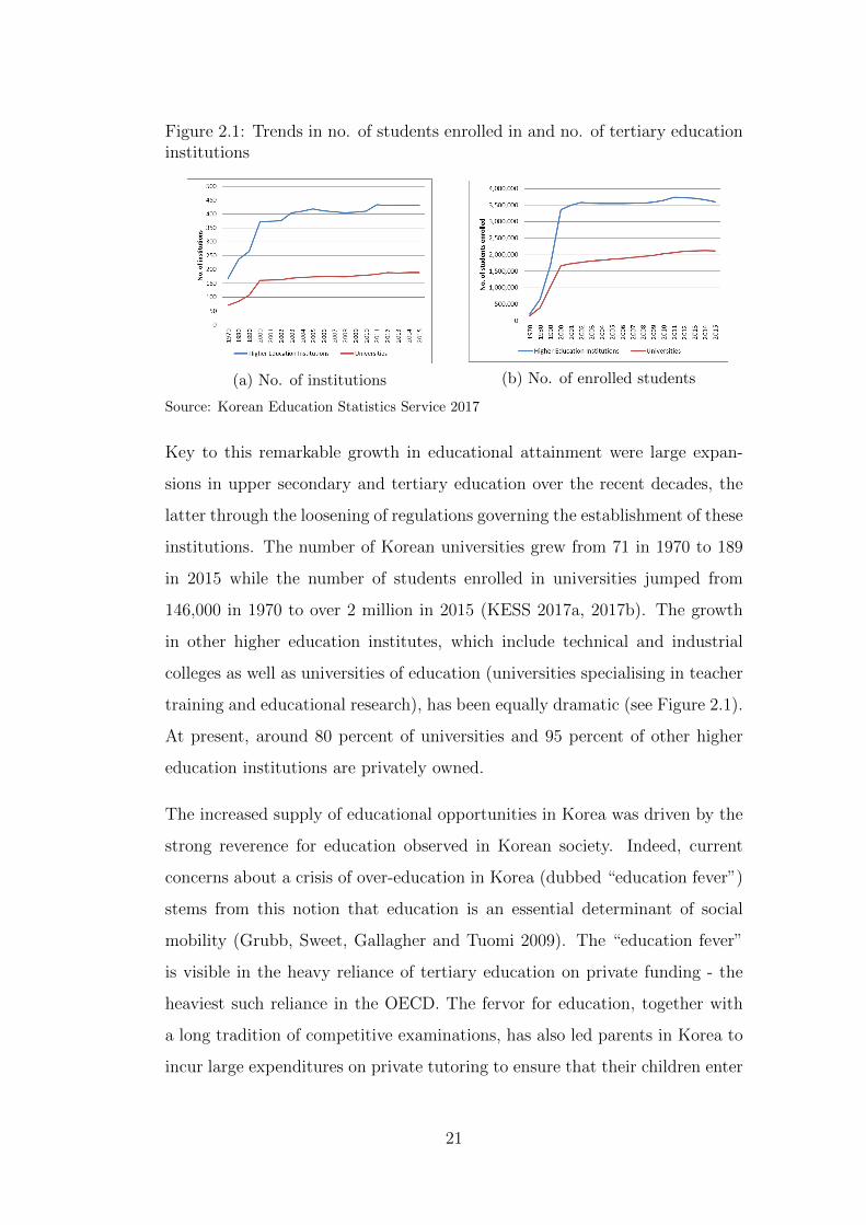
Figure 2.1: Trends in no. of students enrolled in and no. of tertiary educationinstitutions
(a) No. of institutions (b) No. of enrolled students
Source: Korean Education Statistics Service 2017
Key to this remarkable growth in educational attainment were large expan-
sions in upper secondary and tertiary education over the recent decades, the
latter through the loosening of regulations governing the establishment of these
institutions. The number of Korean universities grew from 71 in 1970 to 189
in 2015 while the number of students enrolled in universities jumped from
146,000 in 1970 to over 2 million in 2015 (KESS 2017a, 2017b). The growth
in other higher education institutes, which include technical and industrial
colleges as well as universities of education (universities specialising in teacher
training and educational research), has been equally dramatic (see Figure 2.1).
At present, around 80 percent of universities and 95 percent of other higher
education institutions are privately owned.
The increased supply of educational opportunities in Korea was driven by the
strong reverence for education observed in Korean society. Indeed, current
concerns about a crisis of over-education in Korea (dubbed “education fever”)
stems from this notion that education is an essential determinant of social
mobility (Grubb, Sweet, Gallagher and Tuomi 2009). The “education fever”
is visible in the heavy reliance of tertiary education on private funding - the
heaviest such reliance in the OECD. The fervor for education, together with
a long tradition of competitive examinations, has also led parents in Korea to
incur large expenditures on private tutoring to ensure that their children enter
21

the best schools and universities. It is even conjectured that the unusually low
fertility rates observed in Korea (Korea demonstrated the world’s lowest total
fertility rate of 1.2 in 2014) are a consequence of an extreme quantity-quality
trade-off with huge investments made by parents for the education of their
children (Anderson and Kohler 2013).
Results of the Private Education Expenditure Survey (PEES) provide an
overview of the prevalence of private tutoring in Korea. The total spend-
ing on private tutoring was estimated to be around KRW 17.8 trillion in 2015,
roughly 2 percent of the country’s GDP. Household Income and Expenditure
Surveys reveal that around 5.5 percent of average household expenditure was
accounted for by expenditure on private education other than regular school-
ing. Given that this is an average across all households, for households with
school-going children the fraction is likely to be much higher. 68.8 percent
of all students participated in private tutoring in 2015, spending around 6
hours per week in these additional classes, on average. The main mode of
receiving private tutoring is attending private institutes or Hagwon (which
are widely known for their role as cram schools but which also offer classes
in non-academic subjects) followed by a much lower prevalence of one-to-one
or small-group tutoring. There is also a strong positive correlation between
participation in and expenditure on private tutoring and household income
though private tutoring is by no means rare among the lower income groups -
around a third of children living in households earning less than KRW 1 mil-
lion a month (average household income was 4.3 million KRW) participated
in private tutoring in 2015 (KOSIS 2017c).
State attempts to regulate the private tutoring sector
The importance of the private tutoring industry in Korea has raised concerns
about equity and efficiency leading to several attempts by the state to regu-
late the sector either directly or indirectly. Aside from steps taken to enhance
22

the quality of schooling in general, measures have been taken to reduce the
emphasis on competitive examinations as a means of entry into schools and
universities. The middle school and high school equalisation policies enacted
in 1968 and 1973, respectively, were among the earliest of such measures aimed
at relieving the examination burden on children and the financial burden of
private tutoring on parents. In the regions in which the policies were imple-
mented, entrance examinations to middle schools and high schools were abol-
ished and students assigned to schools randomly based on area of residence.
While it is believed that these policies have reduced the pressure on families
at lower secondary level, it is argued that the competition has now shifted to
university entrance instead (Lee, Lee and Jang 2010). As such, the state has
also engaged in several reforms of the college admissions system including the
introduction of a centralised entrance examination called the College Scholastic
Ability Test (CSAT), increasing college quotas to reduce competition among
students, and encouraging universities to extend their admissions criteria be-
yond CSAT scores to making use of home-school records and implementing
admissions officer systems (Choi and Park 2013).
In addition to these indirect measures, there have also been direct attempts to
control the private tutoring market. The most drastic of these measures was
the 7.30 Educational Reform implemented in 1980 under which the government
banned all forms of private tutoring of a commercial nature. However, given
the difficulty of enforcing the ban, it was gradually relaxed during the 1980s
and 1990s. In 2000, the Korean Constitutional Court ruled that the ban
was unconstitutional, after which the state shifted its focus to enhancing the
quality of schools and regulating the operation and management of Hagwon.
Alongside the establishment of standards on qualifications of instructors and a
mandate to make class fees public information was the regulation on the hours
of operation of Hagwon (Choi and Cho 2016).
The regulation of operating hours of Hagwon falls under the purview of provin-
cial education offices. The imposition of the curfew on closing times of Hagwon
23

Table 2.1: Curfew imposed on Hagwon operating hours for high school stu-dents
Province Curfew Year of New closingimposed imposition time
Seoul Yes 2007 10pmBusan Yes 2008 11pmDaegu Yes 2011 10pmDaejun No - -Incheon Yes 2012 11pmGwangju Yes 2011 10pmUlsan No - -Gyeonggi Yes 2011 10pmGangwona No - -Chungbuk No - -Chungnama No - -Jeonbuk Yes 2009 11pmJeonnam No - -Gyeongbuk No - -Gyeongnam No - -Jeju No - -
Note: The table summarises the imposition of the curfew by provinceincluding the year of imposition and the time at which the curfew was set.a Restriction to close by 10pm was introduced in 2012 but was not imple-mentedSource: Provincial Ordinances
was therefore implemented in different provinces in different years. The curfew
initially varied by the level of school (elementary, middle or high school) though
the goal was to eventually settle on a curfew of 10pm for all students. Prior
to the curfew, the official closing time in all provinces was midnight though it
is reported that classes went on well beyond this limit. Table 2.1 outlines the
implementation of the curfew by province for high school students.
The curfew has been the topic of heated public debate with the key criticism
being levelled against it being the lack of regulation of other types of tutoring
such as one-to-one tutoring. This means that students are able to switch to
alternative forms of tutoring, which would further exacerbate social inequality
given that these alternative forms of tutoring are usually more expensive (Choi
and Choi 2015). However, proponents of the policy argue that the ordinance
24

addresses two major social problems by reducing expenditure on private tutor-
ing and improving students’ health by guaranteeing more sleeping hours (Choi
and Cho 2016). The effects of the curfew are discussed further in Section 2.6.
2.4 Data
This paper uses data from the second wave of the Korean Youth Panel (YP)
collected by the Korean Employment Information Service (KEIS) to estimate
the impact of spending on private tutoring on college entrance outcomes. The
second wave of the YP began in 2007 with a nationally representative sample of
10,206 individuals aged between 15 and 26 in 2007. This sample was followed
every year for eight years (until 2014). The survey collects detailed information
on individual employment, income and education (including detailed informa-
tion about current education of students and the education history of those
adults) as well as information on expenditure on private tutoring by subject
and background characteristics of the household including household income,
parental education, etc.
Using this data I compile a sub-sample of around 2,700 final year, high school
students (roughly 2,200 of these individuals attend general high schools) aged
17 or 18 in their final year of high school, for whom information on private
spending on tutoring and college entrance outcomes for the following year are
available. This covers five cohorts: the high school graduating cohort of 2007
to the high school graduating cohort of 2011. While spending on tutoring over
the total high school period would be the most relevant measure for assessing
effects on college entrance, obtaining this information from the YP dataset
would result in the sample shrinking to 1,320 students. Therefore, for the
analysis, I consider average monthly spending on tutoring in the final year of
high school (in constant 2010 KRW) as the measure of tutoring expenditure.
(Consequences of using this measure are discussed in detail in Section 2.8.)
Since students from vocational or technical high schools (as opposed to general
25

high schools) are less likely to participate in private tutoring and more likely
to attend different types of tutoring classes and higher education institutions
than the general high school students, in the analysis that follows, I consider
separately the full sample and the sub-sample consisting solely of general high
school students. Finally, I consider two different outcomes of college entrance.
These are the enrollment of the student in any higher education institution
(which includes two year colleges, technical or vocational colleges as well as
four year academic universities) and enrollment in a four year college.
The summary statistics for this sample are presented in Table 2.2. As the
table indicates, 53 percent of students in the sample participate in tutoring
during their final year of high school with average spending of roughly KRW
283,000 a month (these figures are comparable to the statistics published in
KOSIS 2017c). Among those who participate in tutoring, average spending is
closer to KRW 530,000. In terms of college outcomes, 78 percent of the sample
attend some type of college in the year after graduating from high school, with
51 percent enrolling in four year colleges. More than 80 percent of the sample
attend general high schools while 42 percent of the students have at least one
parent who has obtained some higher education.
Given the short length of the YP survey and the relatively recent implemen-
tation of the curfew, many of the original sample were still engaged in under-
graduate studies in 2014 (the last year of the survey). As a way of identifying
the effect of tutoring on longer term outcomes, I use the most recent Regional
Labour Force Survey (for 2016) to obtain education and labour market out-
comes for a different but much larger sample of 18,908 individuals, belonging
to the same province-year of birth cohorts represented in the YP sample.4 This
allows for a Two-Sample 2SLS approach which imputes spending on tutoring
in the LFS dataset using first stage estimates from the YP at the province-year
of birth level. The key drawbacks of using this dataset are the lack of fam-
4Since the youngest cohort in the YP sub-sample used in the main analysis attendedtheir final year of high school in 2011 it is reasonable to assume that most of the cohorts inthe YP sample have completed their undergraduate studies by 2016.
26

Table 2.2: Descriptive statistics
Variable Mean Std. Dev.A: Youth Panel sample (N=2,710)Participates in tutoring 0.53 0.50Monthly spending on tutoring 28.26 40.36(in constant 2010 KRW 10,000)Attends any college 0.78 0.42Attends four year college 0.51 0.50Exposed to curfew 0.29 0.45
At least one parent with higher education 0.42 0.49Male 0.55 0.50First born child 0.47 0.50Mother employed 0.58 0.49Father employed 0.94 0.23Attended general high school 0.82 0.38
B: Regional Labour Force Survey sample (N=18,908)Completed four year degree 0.35 0.48Completed any higher education 0.54 0.50Employed 0.56 0.50Monthly wage before tax 165.71 70.58(in constant 2010 KRW10,000) (N=9,958)Exposed to curfew 0.38 0.48
Note: The table presents descriptive statistics of the samples used from the YP and LFS.Sources: Youth Panel, Regional LFS
ily background information and the inability to identify exactly the year and
province in which the respondent completed high school. The issues arising as
a result of these drawbacks and some attempts to address them are described
in the section on robustness checks.
Aside from the YP and LFS data, I use three other datasets to provide ro-
bustness checks for my main analysis: the Korean Youth Risk Behaviour Web-
Based Survey (KYRBS), which provides information on time use among high-
school students; the Private Education Expenditures Survey (PEES), which
provides information on spending on different types of tutoring for high school
students; and the Korean Education and Employment Panel (KEEP) survey,
which includes detailed information on schools and students, including spend-
27

ing on tutoring. The first two datasets are used to further investigate the
impact of the curfew on tutoring expenditure while the third is used to get a
better understanding of the determinants of private tutoring expenditure.
The KYRBS is a national, cross sectional survey carried out annually, starting
from 2005, by the Centre for Disease Control and Prevention to assess health-
risk behaviours among middle and high-school students. Close to 25,000 high
school students are surveyed each year, answering questions related to lifestyle
and health. Particularly useful for this study are the responses on the hours
of sleep and internet usage. The data on hours of sleep are recorded using
a categorical variable in 2005 and 2006, after which the hours of sleep are
recorded as a continuous variable. Information on time spent using the in-
ternet is collected from 2008 onwards. The survey also includes information
on the students’ backgrounds including parental characteristics and type of
high school. I use the KYRBS to assess the impact of the curfew on hours of
sleep and internet usage of high school students as a means of validating the
first stage from my main analysis and confirming that the curfew was indeed
binding.
PEES is a national, cross-sectional survey which, starting from 2007, is carried
out every year, though information on province of residence is available only
from 2009. The survey is administered on parents of students in elementary,
middle and high school, covering information on money and hours spent on
private tutoring for each child as well as some background characteristics. The
dataset also includes expenditure broken down by type of tutoring. PEES
covers a large sample of more than 40,000 high school students each year, of
which roughly 80-85 percent are from general high schools, though the data
does not specify the age or year of high school the student is in. I use this data
to investigate whether any substitution between different types of tutoring
arose as a result of the curfew.
Finally, KEEP is a longitudinal survey that follows two cohorts of students,
2,000 students in the final year of general high school and 2,000 students in the
28

final year of middle school, starting from 2004 and going on for eight years. The
survey collects extensive information on students including student aspirations
and attitudes towards education, assessments of individual student ability by
homeroom teachers, family background characteristics and school information.
Given the longitudinal design of the survey, the study also follows students
through to university or employment. While the dataset is richer than the
YP, its lack of time variation does not allow for its use under my identification
strategy. However, it can provide some insights as to the type of student who
obtains private tutoring and would be most affected by the curfew, which is
useful in interpreting the 2SLS results. Descriptive statistics for these three
supplementary datasets are given in Appendix A1.
Who receives tutoring?
To better understand the characteristics of the students who obtain tutoring,
this section provides some descriptive evidence using the YP and KEEP data,
regressing spending on private tutoring on a set of individual, parental and
school characteristics. These results are presented in Table 2.3.
Qualitatively, the results are fairly similar between the two datasets. House-
hold income and parental education have strong positive associations with
spending on private tutoring in both datasets. The parental employment dum-
mies are not significant in the YP regressions, though this can be explained by
the inclusion of household income as an explanatory variable. The dummies for
being male and being the first born child, which are significant in the KEEP
regressions, are not significant in the YP regressions though they share the
same sign. The impact of school characteristics can be observed through the
KEEP dataset. Unsurprisingly, the pupil-teacher ratio is strongly positively
correlated with private tutoring as is attending a public school.
The KEEP data also includes an assessment by the previous year’s homeroom
29

Table 2.3: Determinants of private tutoring expenditure
Monthly spending on (1) (2) (3) (4)tutoring (in KRW 10,000)Monthly household income 0.003*** 0.003*** 0.0266*** 0.0240***(in KRW 10,000) [0.000] [0.000] [0.00661] [0.00782]At least one parent with 10.112*** 10.037*** 8.158*** 7.671***higher education [2.032] [1.925] [1.433] [1.447]Male -1.849 -2.832 -4.941*** -4.724***
[1.176] [1.800] [1.109] [1.392]First born child 1.295 0.889 4.060*** 5.140***
[0.850] [1.850] [0.789] [1.331]Pupil teacher ratio 0.996** 1.094**
[0.351] [0.449]Public school 1.715 3.039**
[1.379] [1.209]Hours of self study 0.180** 0.151*
[0.0745] [0.0779]Ranking in school -0.0649**(teacher assessed) [0.0285]Mother employed -2.228 -2.675
[1.469] [1.853]Father employed 1.833 2.561
[4.046] [4.476]General high school 18.039***
[3.645]
R-squared 0.298 0.291 0.182 0.188N 2226 1828 2265 1777
Dataset YP - full YP - GHS KEEP KEEP
Notes: The table presents the results of regressing monthly spending on tutoring on indi-vidual, parental and school characteristics using YP and KEEP datasets. Column (1) usesthe full YP dataset while column (2) uses the sample of general high school students. Allregressions include year and province fixed effects and state-specific linear trends.Standard errors clustered by province are given in parentheses. Significance levels: * p < 0.1,** p < 0.05, *** p < 0.01
30

teacher of the student’s percentage rank relative to the rest of the school.5
It appears that students who are ranked higher by their teachers and spend
more hours in self study are also those who spend more on private tutoring.
While these results cannot be interpreted causally, they suggest that those
who would be most affected by the imposition of the curfew would be the high
ability students.
2.5 Empirical strategy
In this section, I describe in detail my identification assumptions and estima-
tion strategy. In particular, I argue that the curfew on operating hours of
Hagwon is a valid instrument for spending on tutoring.
2.5.1 Estimating model
The equation to be estimated is
yist = βPist + γXist + αs + δt + ρst+ uist (2.1)
where yist refers to the outcome of interest for student i who attended school
in province s at time t. The four outcomes I consider are: 1) an indicator
for attending any higher education institution or completing any higher edu-
cation qualification; 2) attending a four year college or completing a four year
degree; 3) being employed; and 4) wages (in natural logarithm). Pist refers
to the monthly expenditure by parents on private tutoring for student i in
his/her final year of high school (in constant 2010 KRW), Xist is a vector of
parental and student characteristics, αs is a region fixed effect, and δt is a
time fixed effect. Since it is a concern that other state-specific trends might be
5It can be argued that this is not a bad control as it is an assessment of the student’sperformance from the previous year as opposed to being an outcome of the tutoring obtainedthis year.
31

correlated with the curfew, I also control for state-specific linear trends, ρst,
in all specifications. The term uist is a random error factor. I also consider
a second specification where an interaction between expenditure on tutoring
and parental education is included.
As mentioned previously, the monthly expenditure on tutoring is most likely
related to school characteristics as well as unobserved parental and student
characteristics such as importance placed on education, ambitions of the par-
ents for child i, the student’s ability and motivation, etc. As a result, estimates
of β through probit or ordinary least squares (OLS) are likely to be biased and
inconsistent.
In this paper, I use the curfew imposed on the operating hours of Hagwon,
which was implemented in different provinces in different years, as a source of
exogenous variation in spending on tutoring. In particular, I consider exposure
to the curfew, measured as interactions between dummy variables indicating
years of exposure to the curfew (determined by the age of the individual)
and the closing time imposed by the curfew, as instruments for tutoring ex-
penditure.6 Since it is very likely that the imposition of curfews in different
regions were based on state- and time- specific factors, identification is based
on the assumption that, conditional on state and time fixed effects and the
state-specific linear trends, the imposition of the curfew was exogenous.
2.5.2 Curfew as an IV
Using the curfew on the operating hours of Hagwon as an instrument for
spending on tutoring requires that the curfew satisfy relevance and validity.
In this section, I consider some issues that might arise from using the curfew
as an IV.
The first issue concerns the first stage. While the curfew needs to have a
6A similar approach is used in Duflo (2001) who uses exposure to a school constructionprogramme in Indonesia as an instrument for years of schooling.
32

significant effect on spending on tutoring, the effect should be negative to
allow the comparison of tutoring expenditure before and after the curfew. To
clarify, it is possible for students to switch to more expensive forms of tutoring
such as one-on-one tutoring or reschedule classes for the weekend as a result
of the curfew on Hagwon operating hours. This would result in expenditures
remaining unchanged or even rising after the imposition of the curfew, which
would be problematic if the quality of tutoring changed as a consequence of the
curfew. It is not possible to completely rule out the possibility of substitutions
away from Hagwon classes but the extent of this problem can be gauged from
the first stage estimates and will be discussed further in Section 2.8.
While the first stage examines the effect of the instrument on the treatment
(here, spending on tutoring), it is not possible to directly test the validity of the
instrument or the existence of other channels by which the curfew may affect
the educational outcomes. For instance, if universities altered their admissions
policies to make special provision for states with a curfew or if families moved to
avoid the constraints of the curfew, the validity of the curfew as an instrument
would be violated. However, given that the curfews were enacted in states with
the highest concentration of educational facilities and private tutoring (the
seven provinces in which the curfew was imposed accounted for 68 percent of
Korea’s total population in 2012), it is unlikely that either of these explanations
bear out. Colleges, if taking regional disparities into consideration, would
be more likely to penalise a student living in a state with a curfew, while a
household that moves for educational purposes would be far more likely to
move into one of these states than out of it. Furthermore, while there is
no evidence to suggest that colleges take province of origin into account when
making admissions decisions, inter-provincial mobility for households with high
school students is very low in Korea. Published statistics on internal migration
in Korea indicate that only 3.6 percent of 15-19 year olds changed their state
of residence in 2016, with just 1 percent moving from a state with a curfew
to one without (KOSIS 2017b). In the Youth Panel sample, only 29 students
(1 percent of the sample) moved out of states with a curfew over the survey
33

period and, of them, only 9 moved after the imposition of the curfew.
Finally, it is important to think about the treatment effect captured by the
estimation. Given that the curfew is for either 10pm or 11pm, the curfew
will only be binding for those students who attend tutoring classes until late
at night and spend heavily on tutoring. The results obtained, therefore, will
be a local effect for those heavy spenders, particularly if there is reason to
believe that the returns to tutoring expenditure are not constant. Based on the
descriptive analysis of the determinants of private spending, it is the students
whose parents are more educated and wealthy that spend more money on
tutoring. The results from the KEEP data are also suggestive of students with
higher ability (as assessed by their teachers) and motivation (as measured by
hours of self-study) spending more on tutoring. As such, it seems plausible
that the effects I estimate are specific to this type of student.
2.6 Effect of the curfew
In this section I investigate the effect of the curfew on Hagwon operating hours
on spending on tutoring. Aside from being the first stage of the IV estimation,
the effect of the curfew is interesting in its own right, highlighting the enormous
investment of time and money devoted to tutoring in Korea.
Table 2.4 presents the results of the first stage. The first stage is estimated
separately for the full sample and the general high school sample. In models
where the regressor of interest (here the exposure to the curfew) is essentially
the interaction of a state and time fixed effect, it is possible that there are
other state-specific trends that might be correlated with the variable. The
state-specific linear trends are an attempt to control for these other trends,
though ideally the results should not change much with their inclusion. In
the regression results presented below, I show results with and without the
inclusion of these trends. All regressions also include dummies for being male,
34

being the first born child, parents’ employment status, and at least one parent
having higher education.7 Standard errors are clustered at the state-year level
- the level of the instrument.
The results indicate that the curfew imposed at 10pm had a significant negative
impact on spending in both the full and general high school samples, while
the 11pm curfew does not seem to have had any effect. Despite the lack of
an effect of the 11pm curfew (which affected 7 percent of the sample), the
joint significance of the curfew exposure dummies is strong, indicating a good
first stage. The inclusion of state-specific trends affects the estimated effects
of the 11pm curfew for the full sample, though the coefficients that change
sign are insignificant in both specifications. Overall, however, it appears that
the inclusion of the trends serves to strengthen the negative effects of the
10pm curfew rather than change them completely. Therefore, in what follows,
I continue to use the specification which includes these state-specific linear
trends.
The negative effect of the 10pm curfew indicates that the direct effect of the
curfew which curtailed spending on tutoring overrode the substitution towards
other types of tutoring as discussed in the previous section, though it still
cannot be ruled out completely. The results also show that the effect of the
curfew increases with the years of exposure to the curfew (the base category
consists of students who did not face any curfew). That is, a student’s spending
on tutoring in her final year of high school depends not only on whether she
lives in a province with a curfew but also on how long she has been exposed to
the curfew. For instance, a student who has been schooling in a province with
a curfew since her first year of high school spent much less in her final year
than a student who was faced with that same curfew only in her final year.
A possible explanation for this is that students (and parents) have adjusted
gradually to spending less on tutoring, with younger cohorts spending less than
7Household income is not included as a control for two reasons: it restricts the samplesize considerably and is most likely to be mis-measured. However, the parental employmentand education indicators should capture most of this effect.
35

Table 2.4: Effect of the curfew on spending on tutoring
Monthly spending on Full sample GHS sampletutoring (in KRW 10,000) (1) (2) (3) (4)
curfew=11pm, years=1 1.675 -1.618 -1.043 -3.728[2.417] [1.496] [2.508] [2.376]
curfew=11pm, years=2 5.094* 0.413 -0.845 -4.407[2.963] [3.993] [2.500] [5.448]
curfew=11pm, years=3 3.2 -0.983 -3.777 -6.954[3.450] [6.764] [3.355] [8.720]
curfew=11pm, years=4 21.457*** 17.218[5.607] [11.095]
curfew=10pm, years=1 -5.123 -3.308 -6.606 -8.036**[5.119] [4.902] [4.302] [3.778]
curfew=10pm, years=2 -11.427** -14.996*** -16.366*** -23.119***[5.240] [5.151] [4.479] [3.905]
curfew=10pm, years=3 -14.570** -23.182*** -18.641*** -30.365***[5.601] [5.482] [4.956] [4.364]
curfew=10pm, years=4 -5.602 -18.875*** -12.416** -28.730***[5.713] [5.693] [5.200] [4.688]
curfew=10pm, years=5 -20.755** -40.473*** -26.186*** -51.180***[9.334] [8.213] [8.363] [7.569]
At least one parent with 13.580*** 13.715*** 14.137*** 14.322***higher education [2.273] [2.308] [2.424] [2.469]Male -1.498 -1.351 -2.377 -2.096
[1.340] [1.335] [1.564] [1.534]First born 0.876 0.658 0.746 0.414
[1.857] [1.869] [2.167] [2.200]Mother employed -1.095 -1.226 -0.979 -1.147
[1.390] [1.389] [1.675] [1.663]Father employed 8.351*** 8.367*** 10.594*** 10.532***
[2.481] [2.518] [3.398] [3.510]Attended general high school 17.514*** 17.284***
[2.463] [2.506]
F-stat 40.14*** 369.89*** 15.64*** 86.99***
State-specific linear trend No Yes No YesN 2710 2710 2231 2231
Notes: The table presents first-stage estimates for the full sample as well as the GHS sample. All regressionsinclude time and state fixed effects and state-specific linear trends.The F-statistics test the hypothesis that the coefficients on the curfew exposure dummies are jointly zero.Standard errors clustered at state*year level given in brackets. Significance levels: * p < 0.1, ** p < 0.05, ***p < 0.01
36

the older cohorts.
By contrast, the 11pm curfew does not seem to have affected tutoring expendi-
ture. This could either be because the 11pm curfew did not constrain spending
or because individuals living in these provinces rescheduled classes or switched
to alternative forms of tutoring. While the former explanation would weaken
the first stage, the latter potentially complicates the interpretation of the ef-
fect of tutoring expenditure before and after the curfew. In Section 2.8 I verify
this using PEES data to examine the impact of the curfew on the spending on
different types of tutoring.
The first stage for the specification where an interaction term between spending
on tutoring and parental education (captured by a dummy variable indicat-
ing that at least one of the parents has completed some higher education) is
included is similar but the inclusion of the interaction term highlights slight dif-
ferences in the response to the curfew by students from different backgrounds.
Figure 2.2 plots the estimated effect of the curfew for each parental education
group against the years of exposure to the curfew. Note that for the less ed-
ucated parents this effect is just the coefficient on the corresponding curfew
dummy whereas for the more educated parents the effect is the sum of the
coefficients on the curfew dummy and interaction term.8
As in the model with no interaction between spending and parental education,
only the 10pm curfew caused a significant reduction in spending on tutoring,
with the size of the effect increasing in the years of exposure to the curfew.
(The points in the graph represented by a marker with no fill are statistically
insignificant.) Children of more educated parents who faced the 10pm curfew
only in their final year of high school do not show a significant decrease in
spending in response to the curfew, and by and large, it seems that more
educated parents reduced their spending by smaller magnitudes than the less
educated parents. Given that more educated parents also spend much more
on tutoring, this suggests some potential substitutions (either in class times or
8The full regression table is available in Appendix A2.
37

Figure 2.2: Effect of the curfew by years of exposure and parental education
Panel A: 10pm curfew
Panel B: 11pm curfew
Notes: The graphs plot the effect of the curfew by years of exposure to the curfew for the two parentaleducation groups and for the two curfews. The effect for the lower education group is given by the regressioncoefficient of the curfew dummy while the effect for the higher education group is the sum of the coefficient ofthe curfew dummy and the coefficient on the interaction between the curfew dummy and education dummy.The two top figures show the effects of the 10pm curfew, while the two bottom figures show the effects ofthe 11pm curfew. Markers with no fill represent effects that are not significantly different from zero at 10%significance.
tutoring type), an issue addressed in the section on robustness checks.
To summarise, I find that the imposition of the 10pm curfew resulted in a
significant reduction in monthly spending on tutoring, while the 11pm curfew
does not seem to have significantly affected tutoring expenditure.9 As such,
the first stage is driven by the effect of the 10pm curfew and the estimated
effects of tutoring expenditure on educational outcomes will be the effects on
those students whose spending was affected by the imposition of the curfew.
The next section, which presents the results of the IV estimates, attempts to
identify these effects.
9This is contrary to the findings of Choi and Choi (2015) and Choi and Cho (2016) whouse data from the Private Education Expenditure Surveys and do not find significant effectsof the curfew. However, both these papers focus on the 2009-2012 period and use differentspecifications for estimating the effects of the curfew. Furthermore, as evinced by the firststage results reported in this paper, while the impact of the curfew strengthens with theduration of exposure to it, the aforementioned papers are unable to use this variation.
38

2.7 Results
In this section, I present and discuss the estimated effects of spending on
private tutoring on educational outcomes. The first part of the analysis is
based solely on the Youth Panel sample and provides estimates of the effect on
entering any higher education institution or entering a four year college.10 I
supplement these results using Regional Labour Force Survey data to estimate
the effect of tutoring expenditure on longer term outcomes such as completing
any higher educational qualification or completing a four year degree, and
being employed.
Despite the dependent variables used in the estimations being binary outcomes,
I use the 2SLS estimator. As explained in Angrist and Pischke (2009), while
non-linear models may fit the conditional expectation function better, linear
IV methods like 2SLS capture the local average treatment effect regardless of
whether the dependent variable is binary, continuous or non-negative.11
2.7.1 Effect of tutoring expenditure on college entrance
The results of the analysis based on the YP sample are presented in Tables 2.5
and 2.6. Table 2.5 presents the results of the specification which is linear in
spending on tutoring while Table 2.6 presents the results of the specification
where spending is also interacted with parental education. OLS results are
presented alongside the 2SLS results and the estimation is carried out for the
full sample as well as the general high school sample.
The results from the linear specification presented in Table 2.5 do not show
a significant relationship between private tutoring expenditures and entering
10Around 30% of the sample attend technical or vocational colleges which typically offertwo year programmes.
11While Stata’s ivprobit command seems like an easy alternative, it would provide incon-sistent estimates given that the spending on tutoring is a non-negative variable and controlfunction estimators (of which ivprobit is one) are only consistent when the endogenous vari-able is continuous (Dong and Lewbel 2015).
39

college. Indeed, even the OLS results do not show any association between
entering any college and spending on tutoring though the effect on entering a
four year university is significant and positive.
The results in Table 2.6 are more interesting. Once the effect of spending on
private tutoring is allowed to differ by parental education, I find that private
tutoring expenditure increases the probability of attending some higher educa-
tion institution at 10 percent significance for children of less educated parents
in the GHS sample. The estimated effect of tutoring expenditure on college
entrance for children of more educated parents is significantly lower and is
not significantly different from zero. The results in Column (6) indicate that
an extra KRW 10,000 spent on a child of less educated parents increases the
probability of her entering some college by 1 percentage point. An increase
in spending by KRW 10,000 corresponds to an increase of roughly 4 percent
from the average level of spending, which means that this estimated effect is
sizeable. However, the estimated effects on entering a four year college are
much smaller and are not significantly different from zero in either sample or
for either parental education group.
40

Table 2.5: Effect of tutoring expenditure on college entrance
Full sample GHS sampleAny college Four year college Any college Four year college
OLS 2SLS OLS 2SLS OLS 2SLS OLS 2SLS(1) (2) (3) (4) (5) (6) (7) (8)
Monthly private spending -0.0001 -0.002 0.001* 0.002 -0.0002 -0.001 0.001** 0.0003on tutoring (in KRW10,000) [0.0002] [0.002] [0.0003] [0.003] [0.0002] [0.003] [0.0003] [0.003]
At least one parent with -0.022 0.002 0.053*** 0.029 -0.019 -0.007 0.055*** 0.061higher education [0.017] [0.037] [0.019] [0.048] [0.019] [0.043] [0.019] [0.054]Male -0.002 -0.005 0.045** 0.047** -0.018 -0.02 0.045** 0.044*
[0.016] [0.016] [0.019] [0.020] [0.017] [0.018] [0.022] [0.023]First born 0.002 0.004 0.036* 0.035* 0.004 0.004 0.039* 0.039**
[0.015] [0.016] [0.019] [0.019] [0.020] [0.021] [0.019] [0.019]Mother employed 0.016 0.014 -0.043* -0.041 0.011 0.01 -0.033 -0.034
[0.018] [0.018] [0.025] [0.026] [0.019] [0.019] [0.023] [0.025]Father employed 0.072 0.086** 0.122*** 0.108** 0.026 0.035 0.138** 0.142**
[0.044] [0.044] [0.044] [0.045] [0.049] [0.049] [0.059] [0.060]Attended general high school 0.117*** 0.148*** 0.319*** 0.289***
[0.032] [0.052] [0.028] [0.062]
Notes: The table presents the estimated effects of tutoring expenditure on college entrance using 2SLS and OLS. The full sample includes 2,710 students whilethe GHS sample includes 2,231 students. Columns (1), (2), (5) and (6) use attending any college as dependent variable while columns (3), (4), (7) and (8) useattending a four year college as dependent variable. All regressions include time and state fixed effects and linear state-specific trends.Standard errors clustered at state*year level given in brackets. Significance levels: * p < 0.1, ** p < 0.05, *** p < 0.01
41
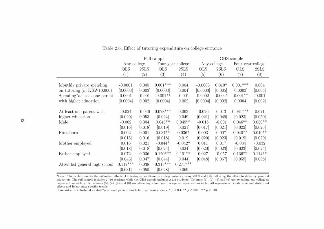
Table 2.6: Effect of tutoring expenditure on college entrance
Full sample GHS sampleAny college Four year college Any college Four year college
OLS 2SLS OLS 2SLS OLS 2SLS OLS 2SLS(1) (2) (3) (4) (5) (6) (7) (8)
Monthly private spending -0.0001 0.005 0.001*** 0.004 -0.0003 0.010* 0.001*** 0.004on tutoring (in KRW10,000) [0.0003] [0.003] [0.0003] [0.004] [0.0003] [0.005] [0.0003] [0.005]Spending*at least one parent 0.0001 -0.001 -0.001** -0.001 0.0002 -0.004* -0.001** -0.001with higher education [0.0004] [0.002] [0.0004] [0.002] [0.0004] [0.002] [0.0004] [0.002]
At least one parent with -0.024 -0.046 0.078*** 0.063 -0.026 0.013 0.081*** 0.071higher education [0.020] [0.053] [0.024] [0.049] [0.021] [0.049] [0.023] [0.050]Male -0.002 0.004 0.045** 0.049** -0.018 -0.001 0.046** 0.050**
[0.016] [0.018] [0.019] [0.021] [0.017] [0.021] [0.022] [0.025]First born 0.002 0.001 0.037** 0.036* 0.003 0.007 0.040** 0.040**
[0.015] [0.016] [0.018] [0.019] [0.020] [0.023] [0.019] [0.020]Mother employed 0.016 0.021 -0.044* -0.042* 0.011 0.017 -0.034 -0.032
[0.018] [0.018] [0.024] [0.024] [0.020] [0.023] [0.023] [0.024]Father employed 0.072 0.036 0.120*** 0.101** 0.027 -0.057 0.136** 0.114**
[0.043] [0.047] [0.044] [0.044] [0.048] [0.067] [0.059] [0.058]Attended general high school 0.117*** 0.038 0.313*** 0.271***
[0.031] [0.055] [0.028] [0.069]
Notes: The table presents the estimated effects of tutoring expenditure on college entrance using 2SLS and OLS allowing the effect to differ by parentaleducation. The full sample includes 2,710 students while the GHS sample includes 2,231 students. Columns (1), (2), (5) and (6) use attending any college asdependent variable while columns (3), (4), (7) and (8) use attending a four year college as dependent variable. All regressions include time and state fixedeffects and linear state-specific trends.Standard errors clustered at state*year level given in brackets. Significance levels: * p < 0.1, ** p < 0.05, *** p < 0.01
42
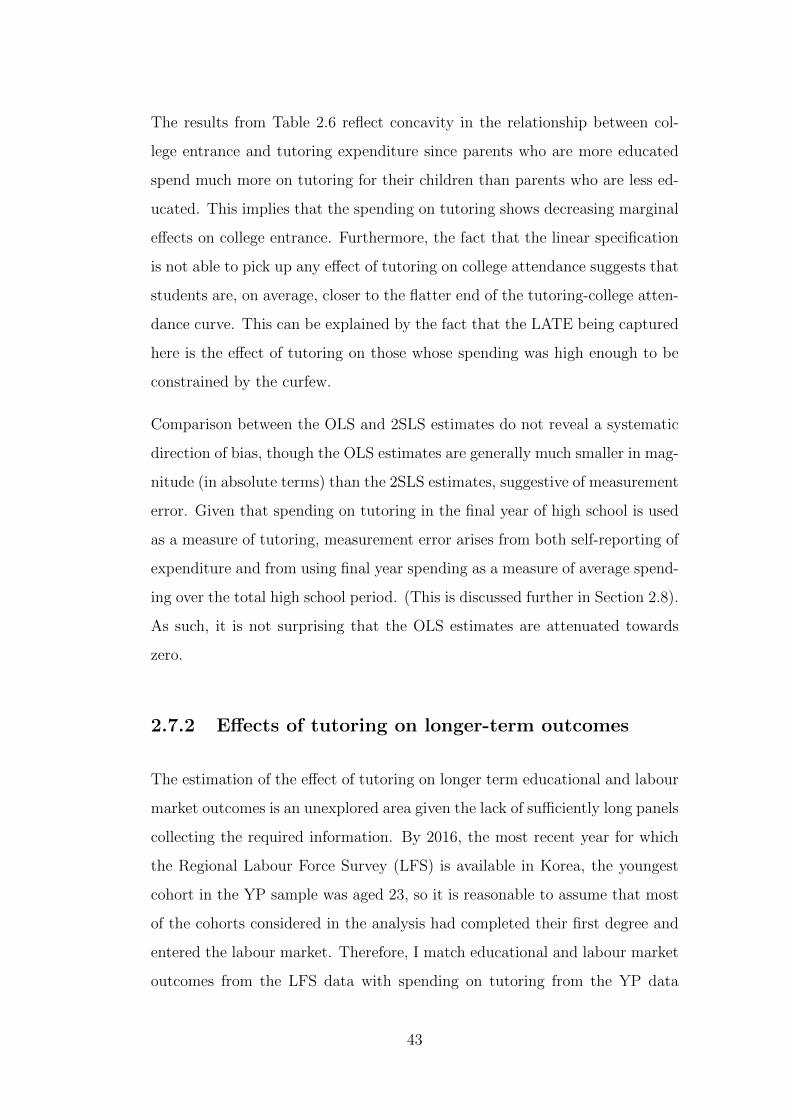
The results from Table 2.6 reflect concavity in the relationship between col-
lege entrance and tutoring expenditure since parents who are more educated
spend much more on tutoring for their children than parents who are less ed-
ucated. This implies that the spending on tutoring shows decreasing marginal
effects on college entrance. Furthermore, the fact that the linear specification
is not able to pick up any effect of tutoring on college attendance suggests that
students are, on average, closer to the flatter end of the tutoring-college atten-
dance curve. This can be explained by the fact that the LATE being captured
here is the effect of tutoring on those whose spending was high enough to be
constrained by the curfew.
Comparison between the OLS and 2SLS estimates do not reveal a systematic
direction of bias, though the OLS estimates are generally much smaller in mag-
nitude (in absolute terms) than the 2SLS estimates, suggestive of measurement
error. Given that spending on tutoring in the final year of high school is used
as a measure of tutoring, measurement error arises from both self-reporting of
expenditure and from using final year spending as a measure of average spend-
ing over the total high school period. (This is discussed further in Section 2.8).
As such, it is not surprising that the OLS estimates are attenuated towards
zero.
2.7.2 Effects of tutoring on longer-term outcomes
The estimation of the effect of tutoring on longer term educational and labour
market outcomes is an unexplored area given the lack of sufficiently long panels
collecting the required information. By 2016, the most recent year for which
the Regional Labour Force Survey (LFS) is available in Korea, the youngest
cohort in the YP sample was aged 23, so it is reasonable to assume that most
of the cohorts considered in the analysis had completed their first degree and
entered the labour market. Therefore, I match educational and labour market
outcomes from the LFS data with spending on tutoring from the YP data
43

to estimate the effect of tutoring expenditure on these longer term outcomes
using two-sample 2SLS (TS2SLS). Put simply, the TS2SLS estimator uses
first stage estimates from the YP data to predict tutoring expenditures at
the province-year of birth level in the LFS sample. In the second stage, the
outcome variables in the LFS data are regressed on predicted expenditure and
the other exogenous controls to obtain the effect of tutoring expenditure on the
outcome. Standard errors are adjusted as prescribed by Pacini and Windmeijer
(2016) to account for the fact that the first-stage estimation was based on a
different sample.
The LFS sample consists of 18,908 individuals born between 1989 and 1993.
Of this sample, 3196 were still engaged in full-time, undergraduate education,
9958 were employed, 1976 were unemployed and the rest were economically
inactive. I consider several different outcomes for this analysis: completion of
a four year degree programme or any higher educational qualification, employ-
ment and wages. When estimating the effect of tutoring on the probability of
completing a higher educational qualification, I exclude full-time undergrad-
uate students from the sample and when estimating the effect of tutoring on
the probability of being employed, I exclude all economically inactive indi-
viduals (which includes the full-time students). However, it should be noted
that the effects estimated without excluding full-time students or the econom-
ically inactive population are hardly different. Given that the LFS does not
include any family background characteristics, the only controls included are
sex, province and year of birth fixed effects and province-specific, linear trends.
Furthermore, I am only able to estimate the linear specification of the model
as given in Equation 2.1. The results of the two-sample 2SLS estimation are
presented in Table 2.7.
These results show a significant, positive effect of spending on tutoring on the
probability of completing a four year degree.12 Here, an increase in tutoring
12While I exclude individuals engaged in full-time undergraduate studies when estimatingthe effects on degree completion, estimating the effects using the entire sample does notsignificantly change the results.
44

Table 2.7: Results of two-sample 2SLS estimation
Dependent variable Spending NCompleted four year degree 0.0039*** 15712
[0.0008]Completed any degree 0.0019* 15712
[0.0011]Employed (=0 if unemployed) 0.0018*** 11934
[0.0004]Employed (=0 if unemployed) 0.0019*** 18908or economically inactive [0.0007]Log wages -0.0004 9958
[0.0012]Notes: The table presents the two-sample 2SLS estimates for four re-gressions; each row corresponds to a different dependent variable. Thecoefficient on spending on tutoring (in 10,000 KRW) for each regressionis given in the second column. The last column indicates how many obser-vations were used in the second stage regression. All estimates are basedon a first-stage regression estimated using YP data on a sample of 2,617individuals. All regressions include a dummy for being male, year of birthand state fixed effects, and linear state-specific trends. Standard errors,clustered at state*year of birth level, are given in brackets.Significance levels: * p < 0.1, ** p < 0.05, *** p < 0.01
expenditure by KRW 10,000 increases the probability of completing a four
year degree by 0.4 percentage points. The estimated effect of completing any
higher educational qualification is smaller and is less precise, though it is still
different from zero at 10 percent significance.
The two labour market outcomes considered in this analysis are being employed
(as opposed to unemployed) and log wages. The results show that individuals
who spent more on private tutoring are more likely to be employed, with
the effect being significantly different from zero at 1 percent level. I do not
find any significant effect of tutoring on wages. However, I do not attach
too much weight to the results from the wage regression for two reasons: the
reduced form of the employment equation indicates strong effects of the curfew
on employment which would lead to selection bias in the estimation of the
wage regression as inclusion in the wage regression sample (being employed) is
significantly affected by the instrument. Second, only half of the LFS sample
is employed in 2016 with roughly 16 percent of the sample still engaged in full
time education, while most of the individuals who are working are only likely
45

to have been working for a few years.
In all, the results point toward positive effects of tutoring on educational out-
comes, though the results vary substantially according to the outcome consid-
ered. The estimation of a model linear in tutoring expenditure reveals a signifi-
cant, positive relationship between tutoring expenditure and completing a four
year degree, with a smaller, less significant effect on completing any degree.
This model does not show any effect of tutoring on college entrance. However,
allowing the effect of tutoring expenditure to differ by parental education re-
veals a large, positive effect of spending on tutoring on entering any college for
children of less educated parents, though the effect for more educated parents
is not significantly different from zero. Even under this specification, I do not
find any significant effect on entering a four year college.
Intuitively, it appears that the linear specification is a better fit for explaining
completion of a four year degree, given that it is a more difficult outcome to
achieve. On the other hand, entering some college is an easier outcome to
reach and so, in the range of spending for which the effects are captured, the
relationship between spending and college entrance is concave. An implication
of the linear specification not being able to pick up any effect of tutoring on
college attendance is that students are, on average, closer to the flatter end of
the tutoring-college attendance curve. Given that the effects captured are for
those whose spending was constrained by the curfew, this is hardly surprising.
The estimated effects of tutoring on labour market outcomes show that while
tutoring expenditure increases the probability of being employed it does not
affect wages. Since spending on tutoring is found to positively affect the proba-
bility of completing a four year degree, it seems reasonable that these graduates
are more employable, giving rise to the positive relationship between tutoring
expenditure and employment. As explained earlier, while the estimates using
log wages potentially suffer from sample selection bias, the lack of an effect of
wages could also be explained by an experience-education trade-off for young
workers as described in Sicherman (1991).
46

2.8 Robustness checks
In this section, I carry out several robustness checks on the relevance and
validity of my identification strategy. In particular, I check the robustness of
my first stage results and examine the effect of the curfew on spending on
different forms of tutoring as well as on hours of sleep and internet usage for
high school students. In addition, I also consider the implications of using
tutoring expenditure in the final year of high school as a measure of the stock
of tutoring obtained over the entire high school period.
2.8.1 Effect of the curfew by type of tutoring
As discussed in Section 2.6, the lack of a significant effect on spending under
the 11pm curfew and the smaller response of more educated parents under
the 10pm curfew could potentially be explained by parents either rescheduling
classes or switching to alternative types of tutoring. To explore this further,
I use the PEES data to examine the impact of the curfew on spending on
different types of tutoring.
I estimate equations similar to the first stage regressions, using expenditure on
the different types of tutoring - Hagwon, one-to-one tutoring and small-group
tutoring - as dependent variables. Given that the PEES data does not indicate
which year of high school a student is in, I use just two dummies to indicate the
curfew at 11pm and the curfew at 10pm. The same set of controls used in the
YP sample is used here, with the exception of the indicator for being the eldest
child which is not available in the PEES data. The results of the regressions
are presented in Table 2.8. It should be kept in mind that the differences in
curfew dummies used and the time periods covered (the PEES dataset spans
from 2009 to 2015 while the YP dataset spans from 2007 to 2011) would lead
to some disparities between the two sets of results though ideally they would
not be too large.
47

The results in Panel A show the estimated effects of the curfew on spending
on different types of tutoring. As in my first stage estimation, while there is a
significant, negative impact of the 10pm curfew on total spending on tutoring,
the effect of the 11pm curfew on spending is not significant. Moreover, the
results from this linear specification indicate that while spending on Hagwon
classes fell significantly as a result of the 10pm curfew, spending on other types
of tutoring were not significantly affected. This confirms that, on average, the
10pm curfew constrained spending on tutoring with little or no substitution
towards other types of tutoring. The results from the general high-school
sample are qualitatively very similar to the results from the full sample, the
only exception being that a significant positive effect on spending on one-to-one
tutoring is recorded under the 11pm curfew in the full sample. In the general
high school sample, however, the 11pm curfew has not changed spending on
any type of tutoring, indicating that the 11pm curfew was not binding.
48
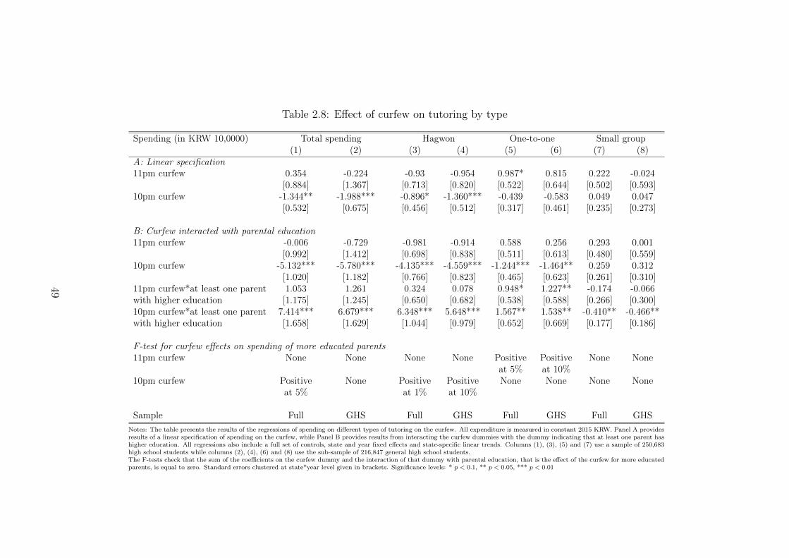
Table 2.8: Effect of curfew on tutoring by type
Spending (in KRW 10,0000) Total spending Hagwon One-to-one Small group(1) (2) (3) (4) (5) (6) (7) (8)
A: Linear specification11pm curfew 0.354 -0.224 -0.93 -0.954 0.987* 0.815 0.222 -0.024
[0.884] [1.367] [0.713] [0.820] [0.522] [0.644] [0.502] [0.593]10pm curfew -1.344** -1.988*** -0.896* -1.360*** -0.439 -0.583 0.049 0.047
[0.532] [0.675] [0.456] [0.512] [0.317] [0.461] [0.235] [0.273]
B: Curfew interacted with parental education11pm curfew -0.006 -0.729 -0.981 -0.914 0.588 0.256 0.293 0.001
[0.992] [1.412] [0.698] [0.838] [0.511] [0.613] [0.480] [0.559]10pm curfew -5.132*** -5.780*** -4.135*** -4.559*** -1.244*** -1.464** 0.259 0.312
[1.020] [1.182] [0.766] [0.823] [0.465] [0.623] [0.261] [0.310]11pm curfew*at least one parent 1.053 1.261 0.324 0.078 0.948* 1.227** -0.174 -0.066with higher education [1.175] [1.245] [0.650] [0.682] [0.538] [0.588] [0.266] [0.300]10pm curfew*at least one parent 7.414*** 6.679*** 6.348*** 5.648*** 1.567** 1.538** -0.410** -0.466**with higher education [1.658] [1.629] [1.044] [0.979] [0.652] [0.669] [0.177] [0.186]
F-test for curfew effects on spending of more educated parents11pm curfew None None None None Positive Positive None None
at 5% at 10%10pm curfew Positive None Positive Positive None None None None
at 5% at 1% at 10%
Sample Full GHS Full GHS Full GHS Full GHS
Notes: The table presents the results of the regressions of spending on different types of tutoring on the curfew. All expenditure is measured in constant 2015 KRW. Panel A providesresults of a linear specification of spending on the curfew, while Panel B provides results from interacting the curfew dummies with the dummy indicating that at least one parent hashigher education. All regressions also include a full set of controls, state and year fixed effects and state-specific linear trends. Columns (1), (3), (5) and (7) use a sample of 250,683high school students while columns (2), (4), (6) and (8) use the sub-sample of 216,847 general high school students.The F-tests check that the sum of the coefficients on the curfew dummy and the interaction of that dummy with parental education, that is the effect of the curfew for more educatedparents, is equal to zero. Standard errors clustered at state*year level given in brackets. Significance levels: * p < 0.1, ** p < 0.05, *** p < 0.01
49

The results in Panel B show the estimated effects of the curfew, allowing the
effect to differ by level of parental education. Again, it appears that only
the 10pm curfew had any significant impact on tutoring expenditure. Less
educated parents spent significantly less on tutoring as a result of the 10pm
curfew, spending less on both Hagwon and one-to-one tutoring, though the
reduction in spending on Hagwon is much larger in magnitude. The effect of
the curfew on more educated parents is quite different. Using F-tests to verify
the overall effects of each curfew on the spending of more educated parents,
it appears that while neither curfew reduced total spending on tutoring by
more educated parents, the 10pm curfew actually caused total expenditure to
rise in the full sample. However, it seems that this is driven by an increase
in spending on Hagwon, pointing to the possibility that, rather than shifting
towards different types of tutoring, more educated parents simply re-scheduled
their children’s classes in Hagwon. I also find a slight increase in one-to-one
tutoring by more educated parents under the 11pm curfew. However, given
that the magnitude of the increase is relatively small (just over KRW 10,000)
compared to average spending on tutoring overall (roughly KRW 200,000), it
is unlikely that the overall quality of tutoring changed very much.
The results from this exercise confirm that the 10pm curfew constrained tu-
toring expenditure, causing spending to decline, while the 11pm curfew did
not and confirms that substitution into alternative forms of tutoring is un-
likely to be a major concern. Rather, it appears that more educated parents
rescheduled extra classes in Hagwon. While this might weaken the first stage,
it would not affect the interpretation of tutoring expenditure before and after
the imposition of the curfew.
50

2.8.2 Effects on time use
As the first stage estimates and the results of the previous section show, only
the 10pm curfew constrained spending on tutoring. As such, the effects cap-
tured in the main analysis are the effects local to those whose spending was
affected by this curfew. In this section, I further explore the effect of the 10pm
curfew, focusing on sleeping hours and internet usage using the Korean Youth
Risk Behaviour Survey. The only channel by which the curfew would affect
time spent sleeping or browsing the internet is through changes to time spent
at Hagwon. Therefore, if spending on tutoring decreased as result of the cur-
few, it would be reasonable to assume that either sleeping hours or internet
usage or both would increase as a consequence of the curfew being imposed.
I regress my measures of time use (hours of sleep on weekdays and minutes of
internet usage on weekdays and weekends) on the set of dummies indicating
exposure to the 10pm curfew and the full set of controls for the sample of final-
year high school students in the same five cohorts as the YP sample (in the
final year of high school between 2007 and 2011). The regressions are carried
out for high school and general high school samples separately and with and
without interacting the curfew dummies with parental education. Note that
the data on internet usage is available only after 2008 and that the dummies on
parental employment status are replaced with measures of the socio-economic
status of the household defined in the KYRBS.
Figure 2.3 plots the effects of the curfew on sleeping hours and minutes of
internet usage on weekdays and weekends for the general high school sample.
The effects for children of more and less educated parents are given by the
blue (solid) and red (dashed) lines, respectively, while the green (dotted) line
gives the average effect. (The full set of results from these regressions as well
as the results for the full sample are available in Appendix A3 and A4.)
The figure shows that sleeping hours and internet usage during weekdays in-
creased significantly, on average, as a result of the curfew being imposed, with
51

Figure 2.3: Effect of the curfew on time use
Notes: The graphs plot the effect of the 10pm curfew on weekday sleeping hours, weekday internet usageand weekend internet usage by year of exposure to the curfew using the GHS sample from the Korean YouthRisk Behaviour Surveys from 2007-2011. Data on internet usage is only available from 2008 onwards. Theeffect for children of less educated parents is given by the red, dashed line while the effect for the childrenof more educated parents (captured by the sum of the coefficient on the curfew dummy and the interactionterm) is given by the blue, solid line. The green, dotted line gives the average effect obtained from theregression model which does not interact the curfew dummies with parental education. Markers with no fillrepresent effects that are not significantly different from zero at 10% significance.
52

the magnitude of the effect on sleep increasing with the years of exposure to
the curfew. In terms of magnitude, the changes in sleeping hours are not very
large, the largest coefficient corresponding to an increase in sleep of around
12 minutes. Note, however, that this is an effect averaged over all students,
including those who get relatively little or no tutoring. The fact that a sig-
nificant effect emerges at all indicates that there is a relatively large number
of students obtaining tutoring until late at night. I also find a large increase
in time spent on the internet during weekdays. These results are reassuring
in that they are consistent with the finding of decreased spending as a result
of the curfew with the size of the reduction increasing with years of exposure
to the curfew. It also appears that internet usage during weekends decreased
significantly after the imposition of the curfew, with the largest reduction of
around 30 minutes. This points to the possibility that some of the tutoring
foregone as a result of the curfew was re-scheduled for the weekend, especially
among the younger cohorts who were exposed to the curfew for longer.
The effects on time use are not systematically different for the two parental
education groups, except for the effects on hours of sleep. The figure indicates
that children of more educated parents experienced larger increases in hours
of sleep than the children of less educated parents. This is not surprising given
that more educated parents spent more on tutoring and were likely to have
been more affected by the imposition of the curfew.
The results of this exercise, which show increased sleeping time and internet
usage after the imposition of the 10pm curfew, are consistent with my first
stage results. Taken together, these results highlight the severity of the college
entrance rat race with students putting in very long hours, even trading off
sleep for additional tutoring.
53
2.8.3 Measurement error in tutoring expenditure
I now address a concern regarding measurement error in tutoring expenditure.
While the IV approach provides a solution for classical measurement error,
using spending on tutoring in the final year of high school as the measure of
total tutoring expenditure over high school brings in a problem of measurement
error different to the errors in self-reporting. The first stage results, which
showed reductions in spending that increased with the years of exposure to
the curfew, suggest that the curfew might have changed the distribution of
tutoring over the three years of high school. If the measurement error caused
by measuring total tutoring expenditure by expenditure incurred in the final
year of high school is related to the instrument, the IV approach will not be
able to eliminate the bias caused by measurement error.
To investigate this issue, I use the smaller sub-sample for which information
on spending over all three years of high school is available to construct the
measurement error (the difference between average spending over all three
years and spending in the final year). I then regress the measurement error on
the average spending over all three years and on the curfew exposure dummies
that I use as instruments. The results of these regressions are presented in
Table 2.9.
The regression results indicate that the measurement error is not correlated to
the average spending over all three years of high school. However, given that
the average spending variable is still subject to the errors in self-reporting, the
results in Columns (1), (2) and (4) should be interpreted with caution. More
important are the results in Column (3). While there are a few curfew dum-
mies which are significantly related to the measurement error, the relationship
does not seem to be systematic. For instance, having lived under the 10pm
curfew for four years decreases the measurement error while having lived under
the same curfew for five years increases it. Therefore, it is likely that the sig-
nificant coefficients are more a result of sampling variation than a systematic
54

Table 2.9: Measurement error in tutoring expenditure
Measurement error (1) (2) (3) (4)
Average spending over 0.041 0.034 0.035all years of HS [0.065] [0.059] [0.059]curfew=11pm, years=1 -1.03 -0.388
[1.320] [1.594]curfew=11pm, years=2 2.485 2.933
[1.906] [1.983]curfew=11pm, years=3 8.452*** 8.852***
[2.692] [2.747]curfew=11pm, years=4 2.081 2.677
[4.334] [4.440]curfew=10pm, years=1 0.945 1.306
[3.526] [3.553]curfew=10pm, years=2 0 0
curfew=10pm, years=3 1.759 1.48[1.320] [1.317]
curfew=10pm, years=4 -2.411** -2.864**[0.922] [1.064]
curfew=10pm, years=5 9.322** 9.082**[3.519] [3.463]
State and year FE No Yes Yes Yes
Notes: The table presents the results of the regressions of the constructed measurementerror in tutoring expenditure on the average spending over all three years of high schooland the curfew exposure dummies for a sample of 1,299 students for whom information onaverage spending over all three years is available. Average spending in measured in KRW10,000. The first column does not include any time or state fixed effects. Standard errorsclustered at state*year level given in brackets.Significance levels: * p < 0.1, ** p < 0.05, *** p < 0.01
relationship between the measurement error and the instruments.
2.8.4 Measurement error in the IV
A key concern arising from the TS2SLS analysis is that the LFS does not
record the year or province in which the respondent completed high school,
but only the province of residence at the time of the survey and year of birth.
This means that the curfew variables will be defined on the basis of province of
residence and year of birth in the LFS dataset. Inter-province migration and
55

early or late graduation would then result in the curfew variable being mis-
measured. It is possible to think of scenarios in which this measurement error
would be correlated with the outcomes (for instance, less academically inclined
students may take longer to graduate high school and will also not attend
college), which means that the measurement error would be non-classical. Now,
when the mis-measurement of the instrument occurs in both samples, the first
stage and reduced form are affected proportionately but the bias cancels out in
the IV estimate even in the case of non-classical measurement error (Pischke
and von Wachter 2008). However, when the measurement error only occurs in
one of the samples, the resulting TS2SLS estimator will also be biased.
It is possible to re-define the curfew variable in the YP sample in terms of the
year of birth of the respondent, rather than her year of high school graduation,
so that this particular source of measurement error, at least, will cancel out in
the TS2SLS estimation. The results presented in Table 2.7 are obtained after
using this correction.13 The measurement error caused by incorrectly inferring
the province of schooling to be the province of residence cannot be dealt with
as easily. However, using statistics on internal migration for young Koreans,
it is possible to get an idea of the magnitude of the problem. In particular,
we need to know the transition matrix for the probability of movement for a
young person between the end of high school and her mid-twenties, between
the three types of provinces on which the instrument is based - provinces with
no curfew, the 11pm curfew and the 10pm curfew.
Using published statistics on internal migration from the Korean Statistical
Information Service (KOSIS), I construct a transition matrix for the proba-
bility of movement between the three types of provinces for individuals aged
20-24 in 2016. This is presented in Table 2.10.14
The table indicates that the probability of staying within a particular type
13This also explains why the sample size for the first stage estimates is smaller than thesample used in the YP 2SLS analysis.
14The full transition matrix broken down for the 16 provinces is available in AppendixA5.
56

Table 2.10: Transition matrix for internal migration for 20-24 year olds
DestinationNo curfew 11pm curfew 10pm curfew
No curfew 0.926 0.017 0.057Origin 11pm curfew 0.029 0.932 0.039
10pm curfew 0.023 0.009 0.968
Notes: The table presents the transition matrix for movement between different provinces,categorised by type of curfew implemented, for individuals aged 20-24 in 2016. The prob-abilities in the diagonal cells are calculated to include those who move between provinceswithin a particular category as well as those who do not move at all. Probabilities arecalculated based on statistics on internal migration by five-year age group and statistics onthe resident population by five-year age group obtained from KOSIS.
of province is high, more than 90 percent in all categories. Those living in a
province with a 10pm curfew are least likely to move (probability less than
4 percent) while those living in a province with no curfew are most likely to
move (probability of roughly 7 percent). Therefore, while there will be some
measurement error in the curfew variable, it is unlikely to be very large. It is
possible to transform the TS2SLS estimates using this transition matrix and
the transition matrix for movements between all 16 provinces. The results after
transformation are very similar to those reported in Table 2.7 (see Appendix
A6 for more details).
2.9 Theoretical framework
In this section, I provide a simple, theoretical model which can provide an
economic intuition for the results presented in the previous section. While my
identification strategy does not allow me to distinguish between signalling and
human capital explanations for the effects of tutoring, the estimated effects
of the curfew on spending on tutoring and sleeping hours, together with the
very fact that a curfew had to be imposed to control spending on private
tutoring, are highly suggestive of rat-race behaviour. As such, I develop a
simple model of asymmetric information with two types of students where
ability is the private information of the student and college admissions are
based on test scores which are signals of ability. The use of signalling models
57

to describe rat-race conditions goes back to Akerlof (1976) who describes a
workplace rat race in which all workers (other than the type with the lowest
productivity) work faster than their optimal speed to signal their productivity
to the employer. This concept of rat-race equilibria is also explicitly presented
as the result of adverse selection by Landers, Rebitzer and Taylor (1996) in an
application to the determination of work hours in law firms.
The model presented here is an adaptation of this asymmetric information
framework to the choice of tutoring and college admissions. The lack of in-
formation on student ability faced by colleges gives rise to a cutoff test score
with students scoring above the cutoff perceived as high ability and admitted
to college. In the separating equilibrium, the cutoff mark is high enough to
discourage low types from getting any tutoring while causing the high types
to obtain more tutoring than would be optimal under perfect information.
After establishing the existence of a rat-race equilibrium, I examine several
comparative statics to illustrate how the rat race may intensify further. This
is similar to the analysis in Hopkins and Kornienko (2010), who illustrate the
effects of changing the inequality of the distribution of rewards (corresponding
to the payoffs from different educational outcomes in this paper) and endow-
ments (corresponding to ability in this paper), on equilibrium outcomes in a
tournament model with a continuum of types. While restricting the model to
just two types and two rewards simplifies the comparative statics considerably,
the broad qualitative conclusions about welfare effects are the same. The only
noteworthy difference is the type of agent affected by changes in the inequality
of these distributions: with a continuum of types, the changes affect lower and
middle types whereas when there are only two types, the changes affect the
high types’ behaviour.
58

2.9.1 The model
Consider an environment in which there are two types of students - high ability
and low ability. Other than for this difference in innate ability, students have
the same endowment of wealth and attend identical schools. Students decide
how much to spend on tutoring, which determines their test scores, with high
ability students having a comparative advantage in the production of test
scores over the low ability students. In addition to tutoring and innate ability,
school quality also positively influences test scores.
The test score, T of type i is given by:
Ti = Ti(mi, S; ai), i ∈ {H,L} (2.2)
where mi ≥ 0 is the amount of tutoring chosen by type i while S is the quality
of schooling and ai is the innate ability of the student. I allow Ti(0, S; ai) > 0
so that students achieve non-zero test scores even with no tutoring. Ti(.) is
strictly increasing and concave in m, S and ai. I allow the function to differ
between types but assume that TH(m;S) > TL(m;S) for all m - that is, for a
given level of tutoring, the high types always receive a higher test score.15
There are two outcomes - attending college or not.16 Students derive utility
from their educational outcome and from consumption (which is equal to the
endowment after spending on tutoring). I assume that the test score is a pure
signal in that students do not derive any utility directly from the test score
though altering the framework so that the test score is a direct source of utility
alongside being a signal of ability will not change the results qualitatively. All
15The key motivation behind allowing the function to differ between types is to allow schoolquality to affect test scores of the two types differently, which makes for more interestingcomparative statics.
16Given that nearly all students in Korea attend some form of higher education the out-comes can also be interpreted as entering a two-year college versus entering a four yearcollege.
59

students have the utility function
U(q, C) = q + C = q + y −m (2.3)
where y is the wealth of the student and q ∈ {q1, q2} corresponds to the payoffs
from not attending and attending college, respectively.
Perfect information
In a setting of perfect information, all high types would be admitted to college,
while low types would not and no one would spend on tutoring. In this perfect
information equilibrium, therefore, low and high type payoffs will be given by:
UL = q1 + y
UH = q2 + y
Asymmetric information
When types are not observable, colleges are no longer able to distinguish high
types from the low and instead use test scores to gauge the ability of a student.
First let us consider the possibility of the perfect information allocation with
neither type spending on tutoring being maintained as an equilibrium. When
neither type gets tutoring high types score higher than low types and it is pos-
sible for the perfect information allocation to be maintained as an equilibrium
so long as the test score high types obtain with no tutoring, TH(0, S; aH), is
high enough to prevent low types from mimicking the high types:17
q1 > q2 −mL(TH(0)) (2.4)
17This feature is usually seen in signalling models in which agents derive utility directlyfrom the signal so that non-zero amounts of the signal are chosen even in the perfect infor-mation setting. In this case, even though students do not derive utility from the test score,the possibility of getting non-zero scores with no tutoring gives rise to this phenomenon.
60

where mL(TH(0)) = T−1L (TH(0); aL) is the amount of tutoring low types need
to reach TH(0, S; aH).18 This might be the case if the difference between high
and low ability is very large or if the difference between q1 and q2 is very small.
For the remainder of this paper, however, I will focus on the more interesting
case in which TH(0) is not high enough to maintain a no-tutoring equilibrium
in the presence of information asymmetry.
When the perfect information allocation can no longer be maintained, there
are two classes of equilibria to consider: pooling and separating. However, we
can use the Intuitive Criterion to rule out all pooling equilibria as well as any
Pareto-dominated separating equilibria. Therefore, I will focus on the Riley
equilibrium of the game in which low types maintain their perfect information
allocation while the high types spend the lowest amount of tutoring that would
prevent low types from mimicking them. This is equivalent to saying that
high types obtain the lowest test score T that does not encourage low types
to deviate.
In general, a separating equilibrium will be characterised by a cutoff score T ′,
which satisfies the following two conditions:
q1 ≥ q2 −mL(T ′) (2.5)
q2 −mH(T ′) > q1 (2.6)
where mi(T′) = T−1
i (T ′; ai) is the level of tutoring required by type i to reach
the test score T ′. Condition 2.5 is the incentive compatibility constraint while
condition 2.6 is the participation constraint.
The Riley equilibrium is the equilibrium in which T ′ = T which is the solution
to:
q1 = q2 −mL(T ) (2.7)
18Since T (.) is a strictly increasing function of m, the inverse is well defined.
61

Note that:
q2 −mH(T ) > q2 −mL(T ) = q1
so that the high types strictly prefer this outcome to pretending to be of
low type. The first inequality follows from the single crossing property where
TH(m) > TL(m) for all m, which implies that mL(T ) > mH(T ) for all T , and
the equality follows from the definition of T .
To summarise, given a low enough TH(0), the equilibrium described in this
section leads to the same outcomes as the perfect information equilibrium for
the low types but the high types will be strictly worse off as they now have to
spend mH(T ) > 0 on tutoring in order to attend college. The higher spending
by high types is supported in the empirical findings with more educated parents
spending more on tutoring in the YP sample (though, of course, children of
more educated parents are not guaranteed to be of type H) and students who
spend more time on self-study and are considered to have greater academic
ability by their teachers spending more on tutoring in the KEEP results.
2.9.2 Comparative statics
I now provide some comparative statics using Equation 2.7 which illustrate how
the rat race for college admission might be aggravated, driving the spending of
high types further up, causing the marginal effects of tutoring they experience
to become smaller.19
Proposition 1. 1. An increase in the payoff to college education, q2, or a
decrease in the payoff associated with no college education, q1, will result
in an increase in T which leads to an increase in mH(T )
19If condition (2.4) were satisfied and the no-tutoring equilibrium is maintained evenwith imperfect information, the comparative statics examined here would be altered so thatchanges currently shown to be causing mH(T ) to rise will instead be changes that lead tocondition (2.4) being violated, giving rise to a new separating equilibrium in which hightypes do have to obtain non-zero tutoring.
62

2. An increase in school quality S will result in an increase in T but the
effect on mH(T ) is ambiguous
Proof. 1. Differentiating Equation 2.7 with respect to q1 and q2 respectively
gives:
(a) ∂T∂q1
= − 1∂mL(T )
∂T
< 0
(b) ∂T∂q2
= 1∂mL(T )
∂T
> 0
since ∂mL(T )
∂T> 0.
mH(T ) is increasing in T so an increase in q2 or a reduction in q1 will
increase spending on tutoring by high types. Since TH = TH(mH , S; aH)
is concave, an increase in mH results in a decrease in ∂TH∂mH
.
2. Differentiating Equation 2.7 with respect to S gives:
∂T
∂S= −∂mL(T )
∂S.
1∂mL(T )
∂T
> 0
Since mH(T ) is the solution to
T = TH(mH(T ), S; aH)
differentiating both sides of this equation with respect to S and rear-
ranging terms gives:
∂mH(T )
∂S= (
∂T
∂S− ∂TH
∂S)
1∂TH∂mH
Since ∂TH∂mH
> 0,
sign(∂mH(T
∂S) = sign(
∂T
∂S− ∂TH
∂S)
63

The first set of effects is fairly intuitive. Higher utility from attending college
or lower utility from not attending college (which can be interpreted as a high
college premium) give the low types greater incentive to deviate from their
equilibrium allocation. As such, the cutoff test score must be high enough to
prevent this. Given that the payoffs from educational outcomes do not enter
the function transforming tutoring into test scores, an increase in T results
directly in an increase in the level of tutoring high types need to reach the
new T , moving the high types further upwards along the tutoring-test score
curve. This result is consistent with that of Hopkins and Kornienko (2010),
who show that increasing the inequality of rewards increases the incentive to
put in extra effort.
The effect of changing school quality on the tutoring expenditure of high types
is ambiguous. An improvement in the quality of schooling will raise test scores
of all students for a given m and so T must rise to satisfy incentive compat-
ibility (Equation 2.7). However, the response of the high types depends on
whether the change in school quality has a larger effect on the cutoff score or
on high type test scores. Note that the cutoff score is determined by low type
behaviour. Therefore, the effect of changing school quality really depends on
the relative importance of schooling in determining the test scores of the two
types. For instance, if the improvement in school quality disproportionately
helps low types, the corresponding rise in T will be larger than the improve-
ments in high-type test scores. In this scenario, we end up in a worse situation,
with the high types having to spend even more as a result of better school qual-
ity. Again, this result is analogous to that in Hopkins and Kornienko (2010)
where a reduction in the inequality of initial endowments makes the low types
more competitive.
Finally, even if an improvement to school quality raises the amount of tutor-
ing consumed by high types, given that school quality is an argument of the
function transforming tutoring into test scores, it is not guaranteed that the
marginal effect of tutoring for high types falls. To see this, note that we are
64

interested in the sign of:
∂
∂S(∂TH∂m|m=mH(T )) =
∂2TH(mH , S)
∂m2H
.∂mH(S)
∂S+∂2TH(mH , S)
∂mH∂S(2.8)
It can be seen that the slope at mH(T ) does not necessarily fall in response to
an improvement in school quality even if mH(T ) increases due to the last term
in Equation 2.8. This term shows how the marginal product of tutoring changes
in response to changes in school quality. It would be positive if schooling and
tutoring were complements and negative if they were substitutes. However, if
the response of mH to a change in S is sufficiently large and positive or if the
complementarity between school and tutoring is sufficiently low for high types,
the marginal effect at the new mH will fall even if tutoring and schooling are
complements. On the other hand, if tutoring and schooling are substitutes, an
increase in S will definitely cause the marginal effect of spending experienced
by high types to fall when ∂mH(T )∂S
> 0.
2.9.3 Discussion
The model of the college admissions rat race presented in this section provides
some economic intuition for the empirical evidence presented in this paper.
The lack of information faced by colleges gives rise to an equilibrium in which
the consumption of tutoring is inefficiently high, particularly among students
of higher ability. While I do not directly estimate the relationship between
student ability and spending on tutoring in this paper, the descriptive results
from the KEEP dataset show positive associations between spending on tutor-
ing and time spent on self-study and academic ability as assessed by teachers.
The results obtained in Section 2.7 provide estimates of the effect of tutoring
expenditure on educational outcomes but cannot distinguish between human
capital and signalling explanations for the results. However, the fact that
colleges in Korea overwhelmingly rely on CSAT scores for making admissions
65

decisions together with the first stage estimates, which highlight large invest-
ments of time and money in tutoring, are highly suggestive of a rat race.
Indeed, the rat race appears to be so severe that students attend classes late
into the night with many students trading off sleep for more hours of tutoring.
As shown in the comparative statics section, a high college wage premium
could explain this large investment in tutoring. Indeed, Machin and McNally
(2007) find that having a tertiary education qualification was associated with a
wage differential of 141 in Korea in 2003 (where the wage of those with a upper
secondary or post upper secondary, non-tertiary qualification was normalised
to a 100), up from 135 in 1998. This is in spite of the large increase in the
supply of tertiary graduates observed over this period.
The comparative statics also suggest that improvements to school quality could
intensify the rat race if said improvements benefited low ability types more
than the high ability types. Many attempts to improve the quality of formal
schooling have been made, alongside the provision of after-school classes by
the schools themselves, to discourage the excessive reliance on tutoring in Ko-
rea. While these efforts certainly benefit students from low-income households,
there is less evidence that they benefit students who are less academically in-
clined. However, if one were to assume that low ability students are less
inclined to spend extra hours on study, it seems intuitive that improvements
to the quality of compulsory schooling would have a higher marginal benefit
for these students.
2.10 Conclusion
In this paper, I provide estimates of the causal effects of tutoring expenditure
on long-term educational and labour market outcomes, using exogenous vari-
ation in private tutoring expenditure caused by the curfew on the operating
hours of Hagwon. I find that while there is a positive effect of tutoring expen-
66

diture on completing a four year degree and on being employed, the effect on
college entrance is subject to decreasing marginal effects. Furthermore, given
that the specification linear in tutoring expenditure is unable to capture any
effect for the average student, it seems that these students are at a flatter part
of the tutoring-college entrance curve. This is explained by the fact that the
LATE estimated in this paper is the effect on those spending large amounts of
money on tutoring, even losing sleep in order to attend more classes.
I then place these empirical findings within an asymmetric information frame-
work to explain how the use of test scores as a signal for ability leads to
inefficiently high investments in tutoring by students of higher ability. In-
creases in the college premium and, under certain conditions, improvements
to overall school quality could exacerbate the situation further by causing the
high types to increase their spending even though the overall outcome, of high
ability types attending college, remains unchanged. The model points to an
inefficient, wasteful equilibrium that arises as a consequence of the rat race
to attend college. The deviation of the individually optimal level of tutoring
from the socially optimal level indicates that some state intervention would
be required to restore the sector to efficient levels of tutoring. However, as
demonstrated in the previous section, certain interventions might make the
situation worse rather than better. While there are high enough payoffs to
having a college degree together with high competition to get into college, it
is unlikely that the rat race can be prevented.
67

Appendices
Appendix A
1 Summary statistics for supplementary datasets
Variable Mean Std. Dev.A: KYRBS sample (N=46,489)Hours of sleep on weekdays 6.44 0.74Internet usage in minutes (N=39,596)
Weekdays 84.26 93.76Weekends 134.89 128.91
Exposure to curfew 0.34 0.47
At least one parent with higher education 0.49 0.50Male 0.51 0.50Household Socio-Economic Status 3.04 0.91(scale of 1-5 where 1 is highest)Attends general high school 0.79 0.41
B: PEES sample (N=250,683)Participates in academic tutoring 0.48 0.50Monthly spending on academic tutoring(in KRW 10,000)
Total 22.51 31.88Spending on Hagwon 12.60 22.94Spending on group tutoring 2.67 10.57Spending on one-on-one tutoring 6.77 19.97
Exposed to curfew 0.55 0.50
At least one parent with higher education 0.55 0.50Male 0.53 0.50Mother employed 0.64 0.48Father employed 0.91 0.28Attends general high school 0.82 0.39
C: KEEP sample (N=2,265)Participates in tutoring 0.57 0.50Monthly spending on tutoring 21.28 33.41
Monthly household income 355.74 239.19At least one parent with higher education 0.35 0.48Pupil teacher ratio in school 15.74 2.16Attends public school 0.47 0.50Teacher assessed ranking in school in previous 42.63 25.71year (N=1,777)Hours of self-study a week 7.56 10.56Male 0.53 0.50First born child 0.54 0.50
Sources: KYRBS, PEES, KEEP
68
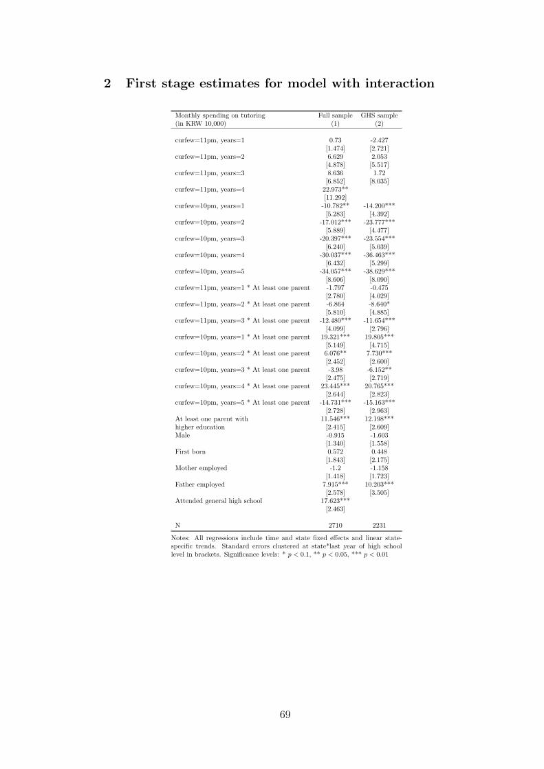
2 First stage estimates for model with interaction
Monthly spending on tutoring Full sample GHS sample(in KRW 10,000) (1) (2)
curfew=11pm, years=1 0.73 -2.427[1.474] [2.721]
curfew=11pm, years=2 6.629 2.053[4.878] [5.517]
curfew=11pm, years=3 8.636 1.72[6.852] [8.035]
curfew=11pm, years=4 22.973**[11.292]
curfew=10pm, years=1 -10.782** -14.200***[5.283] [4.392]
curfew=10pm, years=2 -17.012*** -23.777***[5.889] [4.477]
curfew=10pm, years=3 -20.397*** -23.554***[6.240] [5.039]
curfew=10pm, years=4 -30.037*** -36.463***[6.432] [5.299]
curfew=10pm, years=5 -34.057*** -38.629***[8.606] [8.090]
curfew=11pm, years=1 * At least one parent -1.797 -0.475[2.780] [4.029]
curfew=11pm, years=2 * At least one parent -6.864 -8.640*[5.810] [4.885]
curfew=11pm, years=3 * At least one parent -12.480*** -11.654***[4.099] [2.796]
curfew=10pm, years=1 * At least one parent 19.321*** 19.805***[5.149] [4.715]
curfew=10pm, years=2 * At least one parent 6.076** 7.730***[2.452] [2.600]
curfew=10pm, years=3 * At least one parent -3.98 -6.152**[2.475] [2.719]
curfew=10pm, years=4 * At least one parent 23.445*** 20.765***[2.644] [2.823]
curfew=10pm, years=5 * At least one parent -14.731*** -15.163***[2.728] [2.963]
At least one parent with 11.546*** 12.198***higher education [2.415] [2.609]Male -0.915 -1.603
[1.340] [1.558]First born 0.572 0.448
[1.843] [2.175]Mother employed -1.2 -1.158
[1.418] [1.723]Father employed 7.915*** 10.203***
[2.578] [3.505]Attended general high school 17.623***
[2.463]
N 2710 2231
Notes: All regressions include time and state fixed effects and linear state-specific trends. Standard errors clustered at state*last year of high schoollevel in brackets. Significance levels: * p < 0.1, ** p < 0.05, *** p < 0.01
69

3 Effect of the 10pm curfew on time use
Full sample GHS sampleSleeping hours Internet minutes Internet minutes Sleeping hours Internet minutes Internet minutes
(weekdays) (weekdays) (weekends) (weekdays) (weekdays) (weekends)curfew=10pm, years=1 -0.018 3.211 3.813 0.009 -2.265 -6.217**
[0.035] [2.807] [3.308] [0.025] [1.941] [3.035]curfew=10pm, years=2 0.070* 19.799*** -15.833*** 0.083*** 29.389*** -5.487*
[0.040] [2.074] [2.860] [0.031] [1.876] [2.997]curfew=10pm, years=3 0.082* 27.094*** -4.147 0.127*** 29.305*** -3.744
[0.048] [2.118] [2.818] [0.037] [1.818] [2.990]curfew=10pm, years=4 0.061 17.449*** -15.492*** 0.122** 18.634*** -16.296***
[0.058] [2.962] [4.363] [0.048] [2.412] [4.056]curfew=10pm, years=5 0.102 22.674*** -20.389*** 0.197*** 26.411*** -26.116***
[0.074] [3.875] [6.152] [0.063] [3.081] [5.358]Male 0.145*** 7.888*** 27.707*** 0.113*** 6.055*** 21.721***
[0.010] [1.628] [2.261] [0.010] [1.752] [1.850]Attended general high school -0.145*** -44.067*** -31.148***
[0.019] [4.492] [3.838]At least one parent 0.003 -5.821*** -13.106*** 0.004 -6.136*** -15.111***with higher education [0.012] [1.342] [1.508] [0.013] [1.394] [1.733]2.E SES 0.106*** 7.114*** 21.167*** 0.114*** 4.415* 18.698***
[0.031] [2.434] [3.881] [0.031] [2.626] [3.922]3.E SES 0.100*** 11.209*** 31.341*** 0.114*** 8.648*** 29.071***
[0.027] [2.325] [3.088] [0.028] [2.184] [3.208]4.E SES 0.093*** 20.285*** 49.476*** 0.100*** 17.605*** 49.331***
[0.025] [3.121] [3.645] [0.026] [2.934] [3.642]5.E SES 0.043 22.500*** 50.722*** 0.048 29.000*** 61.930***
[0.033] [3.870] [4.312] [0.037] [4.165] [4.757]
N 46489 39596 39596 36276 31124 31124
Notes: All regressions use data from the Youth Panel and include time and state fixed effects and linear state-specific trends. The first three columns use all final yearhigh school students and the last three columns use only final year high school students in general high schools. Data on internet usage are only available after 2008.Standard errors clustered at state*last year of high school level in brackets. Significance levels: * p < 0.1, ** p < 0.05, *** p < 0.01
70

4 Effect of the 10pm curfew on time use with interac-
tion
Full sample GHS sampleSleeping hours Internet minutes Internet minutes Sleeping hours Internet minutes Internet minutes
(weekdays) (weekdays) (weekends) (weekdays) (weekdays) (weekends)curfew=10pm, years=1 -0.06 2.794 7.364 -0.044 0.748 0.56
[0.039] [3.463] [4.770] [0.028] [3.451] [5.505]curfew=10pm, years=2 0.006 21.860*** -15.503*** -0.029 28.904*** -7.986**
[0.042] [2.063] [2.992] [0.031] [2.053] [3.198]curfew=10pm, years=3 0.038 28.709*** -3.165 0.065* 32.906*** -0.893
[0.050] [2.328] [2.949] [0.039] [2.138] [3.197]curfew=10pm, years=4 0.003 13.452*** -16.872*** 0.074 14.587*** -17.464***
[0.060] [2.993] [4.356] [0.049] [2.542] [4.064]curfew=10pm, years=5 0.076 18.953*** -25.179*** 0.167** 26.197*** -28.979***
[0.075] [3.892] [6.174] [0.064] [3.225] [5.456]curfew=10pm, years=1 0.074*** 0.753 -6.417 0.086*** -4.926 -11.084** At least one parent [0.026] [2.982] [4.541] [0.017] [4.265] [6.226]curfew=10pm, years=2 0.116*** -3.837* -0.649 0.186*** 0.811 4.225*** At least one parent [0.012] [2.018] [1.598] [0.011] [1.725] [1.716]curfew=10pm, years=3 0.073*** -2.805 -1.761 0.097*** -5.883*** -4.688**** At least one parent [0.012] [1.984] [1.606] [0.011] [1.732] [1.712]curfew=10pm, years=4 0.094*** 6.871*** 2.331 0.074*** 6.343*** 1.769* At least one parent [0.012] [1.969] [1.606] [0.012] [1.732] [1.729]curfew=10pm, years=5 0.041*** 5.919*** 7.519*** 0.043*** 0.276 4.178*** At least one parent [0.012] [1.921] [1.612] [0.011] [1.759] [1.706]Male -0.145*** -44.045*** -31.119***
[0.019] [4.493] [3.843]Attended general high school 0.145*** 7.874*** 27.695*** 0.113*** 6.046*** 21.733***
[0.010] [1.633] [2.259] [0.010] [1.755] [1.845]At least one parent -0.016 -6.179*** -12.916*** -0.021* -5.799*** -14.446***with higher education [0.012] [1.740] [1.732] [0.012] [1.639] [1.740]2.E SES 0.106*** 7.106*** 21.207*** 0.114*** 4.454* 18.778***
[0.031] [2.433] [3.882] [0.031] [2.629] [3.922]3.E SES 0.101*** 11.240*** 31.356*** 0.115*** 8.659*** 29.073***
[0.027] [2.337] [3.095] [0.028] [2.195] [3.207]4.E SES 0.094*** 20.315*** 49.505*** 0.102*** 17.613*** 49.339***
[0.026] [3.137] [3.648] [0.026] [2.949] [3.643]5.E SES 0.044 22.491*** 50.707*** 0.048 28.986*** 61.897***
[0.033] [3.879] [4.313] [0.038] [4.155] [4.747]
N 46489 39596 39596 36276 31124 31124
Notes: All regressions use data on final year high school students from the KYRBS 2007-2011 and include time and state fixed effects and linear state-specifictrends.The first three columns use all final year high school students and the last three columns use only final year high school students in general high schools.Standard errors clustered at state*last year of high school level are given in brackets.Significance levels: * p < 0.1, ** p < 0.05, *** p < 0.01
71

5 Transition matrix by province
DestinationSeoul Busan Daegu Incheon Gwangju Daejeon Ulsan Sejong Gyeonggi Gangwon Chungbuk Chungnam Jeonbuk Jeonnam Gyeongbuk Gyeongnam Jeju
Seoul 0.928 0.003 0.002 0.005 0.002 0.002 0.001 0.001 0.037 0.004 0.002 0.003 0.002 0.002 0.002 0.003 0.001Busan 0.016 0.929 0.003 0.002 0.001 0.001 0.006 0.000 0.008 0.001 0.001 0.002 0.001 0.002 0.005 0.023 0.001Daegu 0.016 0.004 0.931 0.002 0.000 0.001 0.003 0.000 0.009 0.001 0.001 0.002 0.000 0.001 0.023 0.005 0.001Incheon 0.017 0.001 0.001 0.937 0.001 0.001 0.001 0.000 0.025 0.003 0.002 0.004 0.002 0.001 0.002 0.001 0.001Gwangju 0.024 0.002 0.001 0.003 0.909 0.002 0.000 0.001 0.014 0.002 0.001 0.002 0.006 0.031 0.001 0.001 0.001Daejeon 0.027 0.002 0.002 0.003 0.001 0.898 0.001 0.010 0.017 0.003 0.008 0.017 0.004 0.002 0.003 0.002 0.001Ulsan 0.021 0.020 0.006 0.002 0.001 0.002 0.913 0.000 0.008 0.002 0.001 0.002 0.001 0.001 0.010 0.010 0.001Sejong 0.032 0.003 0.001 0.005 0.001 0.035 0.001 0.839 0.023 0.002 0.019 0.025 0.004 0.002 0.003 0.002 0.001
Origin Gyeonggi 0.026 0.002 0.001 0.006 0.001 0.002 0.001 0.001 0.943 0.004 0.003 0.004 0.002 0.001 0.002 0.002 0.001Gangwon 0.040 0.004 0.003 0.009 0.001 0.003 0.001 0.001 0.039 0.878 0.006 0.004 0.002 0.001 0.005 0.003 0.001Chungbuk 0.027 0.002 0.002 0.005 0.001 0.012 0.001 0.004 0.025 0.005 0.900 0.007 0.002 0.001 0.004 0.002 0.001Chungnam 0.029 0.002 0.001 0.006 0.002 0.018 0.001 0.004 0.028 0.003 0.005 0.888 0.004 0.002 0.003 0.002 0.001Jeonbuk 0.027 0.002 0.001 0.004 0.007 0.006 0.001 0.001 0.020 0.002 0.002 0.006 0.913 0.005 0.002 0.002 0.001Jeonnam 0.028 0.005 0.001 0.005 0.035 0.003 0.001 0.000 0.021 0.002 0.002 0.004 0.007 0.879 0.002 0.004 0.001Gyeongbuk 0.023 0.010 0.026 0.003 0.001 0.004 0.005 0.000 0.016 0.003 0.004 0.003 0.001 0.001 0.892 0.006 0.001Gyeongnam-do 0.020 0.029 0.005 0.002 0.001 0.002 0.004 0.000 0.010 0.002 0.002 0.002 0.001 0.002 0.005 0.912 0.001Jeju 0.029 0.006 0.003 0.004 0.002 0.002 0.001 0.000 0.017 0.002 0.002 0.002 0.002 0.003 0.002 0.003 0.921
Notes: The table presents the transition matrix for movement between different provinces for individuals aged 20-24 in 2016. The probability in the diagonal cells are calculated to include those who move within the province as well as thosewho do not move at all. Probabilities calculated based on statistics on internal migration by five-year age group and statistics on resident population by five-year age group obtain from KOSIS (www.kosis.kr).
72

6 Correction for internal migration for TS2SLS results
First, consider TS2SLS estimation with no measurement error. Consider a
scenario in which the outcome Y and endogenous treatment x are not observed
together in the same dataset but an instrument Z is observed in both samples.
Let Z1 and Y1 be observed in sample 1 which includes n1 observations and Z2
and X2 be observed in sample 2 which includes n2 observations. In this case,
βTS2SLS is calculated as:
βTS2SLS = (X ′1X1)−1X ′1Y1 (2.9)
= (π′x2Z′1Z1πx2)
−1π′x2Z′1Z1Y1 (2.10)
= (π′x2Z′1Z1πx2)
−1π′x2Z′1Z1πy1 (2.11)
where πx2 is the first stage estimate from sample 2 and πy1 is the reduced form
estimate from sample 1.
A consequence of the instrument being mis-measured in Sample 1 is that the
reduced form estimates (and second stage estimates) will be biased. In the
context of this paper, inferring state of attending high school with the state of
residence is the cause of measurement error. We now use the transition matrix
for migration between provinces for individuals of the corresponding age group
to correct these biased, reduced-form estimates.20
Say, for instance, that πy1,j is the effect of living in state j on educational
outcomes. However, what we want to know is π∗y1,i which is the effect of
finishing school in state i on educational outcomes. The two effects are related
by:
π∗y1,i =∑j
πy1,j.pji (2.12)
where pji is the probability of the individual having finished school in state i
given that he is currently living in state j. If P is a matrix whose i, j element
is pji, the vector πy1 is related to the true effects vector π∗y1 by π∗y1 = Pπy1 .
20The procedure described here borrows from Card and Krueger (1992).
73
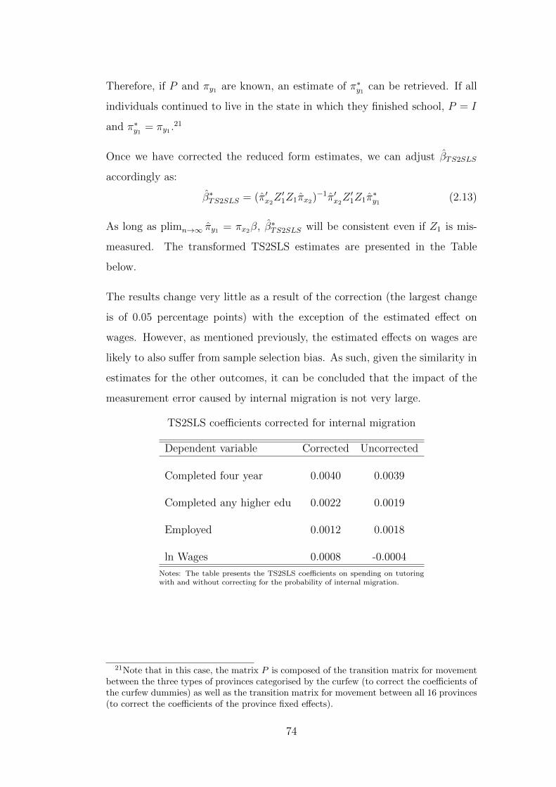
Therefore, if P and πy1 are known, an estimate of π∗y1 can be retrieved. If all
individuals continued to live in the state in which they finished school, P = I
and π∗y1 = πy1 .21
Once we have corrected the reduced form estimates, we can adjust βTS2SLS
accordingly as:
β∗TS2SLS = (π′x2Z′1Z1πx2)
−1π′x2Z′1Z1π
∗y1
(2.13)
As long as plimn→∞ πy1 = πx2β, β∗TS2SLS will be consistent even if Z1 is mis-
measured. The transformed TS2SLS estimates are presented in the Table
below.
The results change very little as a result of the correction (the largest change
is of 0.05 percentage points) with the exception of the estimated effect on
wages. However, as mentioned previously, the estimated effects on wages are
likely to also suffer from sample selection bias. As such, given the similarity in
estimates for the other outcomes, it can be concluded that the impact of the
measurement error caused by internal migration is not very large.
TS2SLS coefficients corrected for internal migration
Dependent variable Corrected Uncorrected
Completed four year 0.0040 0.0039
Completed any higher edu 0.0022 0.0019
Employed 0.0012 0.0018
ln Wages 0.0008 -0.0004
Notes: The table presents the TS2SLS coefficients on spending on tutoringwith and without correcting for the probability of internal migration.
21Note that in this case, the matrix P is composed of the transition matrix for movementbetween the three types of provinces categorised by the curfew (to correct the coefficients ofthe curfew dummies) as well as the transition matrix for movement between all 16 provinces(to correct the coefficients of the province fixed effects).
74
Chapter 3
Population Control Policies and
Fertility Convergence
3.1 Introduction
In the middle of the twentieth century, almost all developing countries ex-
perienced a significant increase in life expectancy, which, together with high
fertility rates, led to rapid population growth rates. The fear of a population
explosion lent impetus to what effectively became a global population-control
programme. The initiative, propelled in its beginnings by intellectual elites in
the United States, Sweden, and some developing countries, most notably India,
mobilised international private foundations as well as national governmental
and nongovernmental organizations to advocate and enact policies aimed at
reducing fertility. By 1976, following the preparation of the World Population
Plan of Action at the World Population Conference in Bucharest in 1974, 40
countries, accounting for 58 percent of the world’s population and virtually
all of the larger developing countries, had explicit policies to reduce fertility
rates. Between 1976 and 2013, the number of countries with direct govern-
ment support for family planning rose to 160. In this essay, we will argue that
concerted population control policies implemented in developing countries are
75

likely to have played a central role in the global decline in fertility rates in
recent decades and can explain some patterns of that fertility decline that are
not well accounted for by other socioeconomic factors.
To set the stage, we begin by reviewing some trends and patterns in the fertility
decline in the last half-century across countries and regions. We argue that
although socioeconomic factors do play an important role in the worldwide
fertility decline, they are far from sufficient to account for the timing and speed
of the decline over the past four decades. For example, the cross-country data
in any given year show a negative correlation between per capita income and
fertility rates. However, that relationship has shifted downward considerably
over time: today the typical woman has, on average, two fewer children than
the typical woman living in a country at a similar level of development in 1960.
We then discuss the evolution of global population-control policies in more
detail. All population-control programmes involved two main elements: pro-
moting an increase in information about and availability of contraceptive meth-
ods, and creating public campaigns aimed at establishing a new small-family
norm. The evidence suggests that these public campaigns appeared to have
been critical in complementing contraceptive provision. While estimating the
causal effects of these programmes is challenging, we examine the relationship
between different measures of family planning programme intensity and the
declines in fertility over the past decades and find a strong association, after
controlling for other potential explanatory variables such as GDP, schooling,
urbanisation, and mortality rates.
In a final section, we discuss in more detail the role played by these other
variables in the decline in fertility and highlight that the drop in fertility rates
seems to be occurring and converging across countries with varying levels of
urbanisation, education, infant mortality, and so on. We conclude that popu-
lation control policies seem to be the factor that best accounts for this com-
monality.
76

Figure 3.1: Fertility histograms over time
0.0
5.1
.15
.2.2
5
Fra
ctio
n
0 2 4 6 8
1960
0.0
5.1
.15
.2.2
5
Fra
ctio
n
0 2 4 6 8
1970
0.0
5.1
.15
.2.2
5
Fra
ctio
n
0 2 4 6 8
1980
0.0
5.1
.15
.2.2
5
Fra
ction
0 2 4 6 8
TFR
1990
0.0
5.1
.15
.2.2
5
Fra
ction
0 2 4 6 8
TFR
2000
0.0
5.1
.15
.2.2
5
Fra
ction
0 2 4 6 8
TFR
2013
Source: The data comes from the World Bank’s World Development Indicators database.Note: The figure shows fertility histograms at the beginning of each decade. In the final histogram, the year2013 is used rather than 2010 to report the latest available information.
3.2 Fertility patterns across time and space
The world’s total fertility rate declined from over 5.0 children per woman in
1960 to 2.5 children per woman in 2013.1 This trend is not driven by just a few
countries. Figure 3.1 plots fertility rate histograms for the start of decades since
1960; the bars show the fraction of countries for each fertility interval. (The
figure shows 2013 rather than 2010 to report the most recent information.) In
1960, more half the countries in the world had a fertility rate between 6 and 8,
and the median fertility rate was 6.2 children per woman. (When weighted by
population, the world’s median is 5.8.) In 2013, the largest mass of countries
is concentrated around 2, with the median total fertility rate being 2.2.
These large declines in fertility took place in most regions of the world, as
1The total fertility rate is defined as the number of children that would be born toa woman if she were to live to the end of her childbearing years and bear children inaccordance with current age-specific fertility rates. In this paper, we will use “total fertilityrate” interchangeably with “fertility” and “fertility rate.”
77

Figure 3.2: Fertility trends across regions
Note: This figure plots the trends in fertility by region, as defined by the World Bank, between 1960 and2013. The data comes from the World Development Indicators database.
shown in Figure 3.2. Between 1960 and 2013, fertility rates fell from 5.4 to
1.81 in East Asia and the Pacific, from 5.98 to 2.16 in Latin America and
the Caribbean, from 6.87 to 2.83 in the Middle East and North Africa, and
from 6.02 to 2.56 in South Asia. The fertility decline in sub-Saharan Africa
has been slower, but still sizeable: since the 1980s, the total fertility rate in
this region fell from 6.7 to 5. Within this region, South Africa has already
reached a total fertility rate of 2.4 and Mauritius is now at a fertility rate of
1.44. While absolute declines in fertility were not as large in North America
or Europe and Central Asia, the percentage declines in both regions have been
significant — nearly 50 percent in North America and close to 40 percent in
Europe and Central Asia. Interestingly, the fertility rate for North America
bottomed out in the 1980s, and in Europe and Central Asia, it bottomed out
in the 1990s.
A number of empirical studies have documented a negative relationship be-
tween fertility rates and income. While this relationship is indeed negative in
the cross-section of countries, the relationship has changed over time, shifting
78

Figure 3.3: Fertility – income relation in 1960 and 2013
Source: Authors using data from the World Development Indicators database.Note: For a sample of 88 countries, the figure shows the scatterplots and fitted line (that is, the lowesssmoothed relationship or locally weighted smoothing function) between the total fertility rate and log of percapita GDP (in constant 2005 US$) in 1960 and 2013. The x-axis is log scale.
downward and becoming flatter over time. Figure 3.3 shows the relationship
between the total fertility rate and real GDP per capita in 1960 and in 2013.
The figure also shows fitted lines for these two years. The downward shift has
been, on average, around 2 children per woman, meaning that today a woman
has 2 fewer children than a woman living in a country at the same level of
development in 1960, which is close in magnitude to the drop in overall world
fertility of 2.5 children per woman. The cross-section relationship between fer-
tility and income observed in 1960 would predict a total fertility rate of around
4 at the average per capita GDP for 2013 (recall the actual rate is 2.5).
As Figure 3.3 illustrates, the issue is not just to explain a decline in global
fertility. It is also necessary to explain why the fall in fertility rates witnessed
by developing countries in recent decades was so very rapid, compared with the
rather slow and secular decline in fertility rates experienced by more mature
economies. For example, the fertility decline began as early as the mid-1700s
in some European countries and only reached replacement levels in the early
twentieth century (Coale 1969). Furthermore, it is necessary to explain why
79

countries with markedly different levels of income, urbanisation, education, and
other factors are all converging to very similar fertility rates. As we discuss in
the next section, the worldwide spread of population-control programmes can
help to explain these patterns in the fertility data.
3.3 The global family planning movement and
its consequences
The following section provides a brief overview of the global family planning
programme, discussing the historical context as well as outlining some of its
characteristics. We then examine more systematically the link between fertility
policy adoption and declines in fertility.2
3.3.1 Global evolution of family planning programmes
After World War II, there was growing concern with the unprecedented lev-
els of population growth. A population-control movement developed, led by,
among others, John D. Rockefeller III, whose main preoccupations were the
growing imbalance between population and resource growth, and the potential
for political instability given that most of the population growth was concen-
trated in the poorest countries of the world. In 1952, Rockefeller founded the
Population Council, aimed at providing research and technical assistance for
population programmes across the world. That same year, India started the
first national population programme, and in parallel, the International Planned
Parenthood Federation was established.3 By the late 1950s, the “population
question” was receiving the attention of the US government. A report by a
2This section draws heavily on Robinson and Ross (2007), who provide a compilation ofcase studies of family planning programmes in 22 countries across the world.
3The earlier birth-control movement led by Margaret Sanger in the United States (whoset up the first birth-control clinic in the United States in 1916) and Elise Ottesen-Jensenin Sweden was another force leading to efforts for fertility reduction.
80

Presidential Committee studying the United States Military Assistance Pro-
gramme (Draper 1959) devoted an entire chapter to the issue, ending with a
recommendation that the government “assist those countries with which it is
cooperating in economic aid programs, on request, in the formulation of their
plans designed to deal with the problem of rapid population growth.”4 By this
time, private foundations including the Rockefeller and Ford Foundations were
providing seed funding for research and planning programmes, but it was in
the mid-1960s that large-scale funding became available and the population
planning movement really took off.
The first large-scale intervention was carried out by the Swedish government,
which supported family planning efforts in Sri Lanka (then Ceylon), India, and
Pakistan, starting in 1962 (Sinding 2007). Over time, several international or-
ganisations, like USAID and the World Bank, joined in providing funds and
support for family planning programmes around the world. The invention of
the modern intra-uterine device (IUD) and the oral contraceptive pill around
the same time allowed for the possibility of easy-to-use and effective contra-
ceptive methods becoming widely available for public use.
These early family planning efforts showed rapid effects in East Asian coun-
tries, including Hong Kong, South Korea, Singapore, and Thailand. Pro-
gramme implementation and success would take longer in other developing
countries, partly due to the difficulty of overcoming cultural inhibitions and
religious opposition towards birth control, as well as operational problems
including inadequate transport infrastructure and insufficient funding. The
World Population Conference in 1974 appeared to be a turning point for the
global family planning movement. Tables 3.1 and 3.2 show how countries
around the world have been categorised by their fertility goals and the type of
government support for family planning for selected years from 1976 to 2013,
according to the UN World Population Policy database.
4For more references that trace the origins of the population control movement primarilyto the West, see Appendix B.
81

Table 3.1: Number of countries with government goals for fertility policy
Year Lower Maintain No Raise Totalfertility fertility intervention fertility
1976 40 19 78 13 1501986 54 16 75 19 1641996 82 19 65 27 1932005 78 31 47 38 1942013 84 33 26 54 197
Source: The data is obtained from the UN World Population Policies database.Note: The table shows the number of countries by type of policy adopted towards fertility.The data begins in 1976. Countries are categorised according to whether they had a policyto lower, maintain, or raise fertility or if they had no intervention to change fertility.
Table 3.2: Number of countries by government support for family planning
Year Direct Indirect No Limit/Not Totalsupport support support permitted
1976 95 17 28 10 1501986 117 22 18 7 1641996 143 18 26 2 1932005 143 35 15 1 1942013 160 20 16 1 197
Source: The data is obtained from the UN World Population Policies database.Note: The table shows the number of countries by the type of support extended by thestate for family planning services. The data begins in 1976. Countries are categorisedby whether their governments directly supported, indirectly supported, or did notsupport family planning as well as if the government limited family planning servicesor did not permit family planning in the country.
In 1976, for example, the 40 countries that had explicit policies to limit fertility
covered nearly one-third of East Asian countries, a quarter of Latin American
and Caribbean countries, and nearly two-thirds of South Asian countries. By
contrast, only one-fifth of countries in North Africa, the Middle East, and Sub-
Saharan Africa had a fertility reduction policy in 1976. By 1996, 82 countries
had a fertility reduction policy in place (by this time, some countries had
reached their fertility reduction targets and changed to policies of maintaining
fertility rates), including half of the countries in East Asia and Latin America,
and more than two-thirds of the countries in Sub-Saharan Africa and South
Asia. These countries represent 70 percent of the world’s population. In 1976,
95 governments were providing direct support for family planning. (Support
for family planning was not always associated with an explicitly stated goal
82

of reducing fertility.) The number of countries with state support for family
planning has continued to rise steadily.
3.3.2 Features of family planning programmes
The early phases of family planning programmes in most developing countries
typically sought to provide a range of contraception methods — some com-
bination of oral contraceptives, IUD, condoms, sterilisation, and abortion —
and information on their use. However, increases in the supply of contracep-
tives proved insufficient to lower fertility rates to desired levels, particularly
in poorer or more traditional societies. This failure led to concerted efforts
to change public attitudes and beliefs and establish a new small-family norm
through active mass-media campaigns. We discuss these two phases in turn.
The implementation of the family planning programmes varied vastly across
countries. Differences included the role of public and private provision; the
price at which contraception was offered; subsidies to production or sales; the
delivery system through which services were provided; the outlets for the mass-
media campaigns; and the various supplementary policies that accompanied
the core measures (Freedman and Berelson 1976).5
Most countries began their family planning programmes with a clinic-based
approach that took advantage of the existing health infrastructure to provide
modern contraceptive methods. Many countries also implemented programmes
in hospitals to advise women on the use of contraception, often after women
had given birth or undergone an abortion. However, this approach had limited
success in countries where a large proportion of women gave birth outside of
the formal health care system, like India and Iran. Thus, the policy was
supplemented by the deployment of trained field workers who made house
calls, particularly in rural areas. In some nations, such as Iran and Malaysia,
5For a more detailed summary of the key features of early family planning programmesaround the world, highlighting the countries that implemented each approach, see AppendixC1.
83

family-planning programmes were linked to maternal and child health services
at an early stage, which allowed for better integration of the programme into
the country’s health system. Towards the 1990s, with the re-branding of family
planning as sexual and reproductive wellbeing, more countries have followed
this approach.
Many of the family planning programmes established in the 1950s and 1960s,
which focused on increasing the supply of contraception, failed to gain much
traction. For instance, highly traditional societies and countries with a pre-
dominantly Catholic or Muslim population had difficulty gaining wide accep-
tance for their family planning programmes. It became clear that without
changing the willingness to use contraceptives and, more importantly, reducing
the desired number of children, merely improving access to birth control had
limited impact. The importance of changing the desired number of children, in
particular, was highlighted by leading demographers at the time such as Enke
(1960) and Davis (1967), who argued that a desire to use contraceptives was
perfectly compatible with high fertility. Countries thus began to present and
to adapt their population-control policies to address these concerns.
For example, early in Indonesia’s family planning programme, the government
published a pamphlet titled “Views of Religions on Family Planning,” which
documented the general acceptance of family planning by four of Indonesia’s
five official religions — Islam, Hinduism, and Protestant and Catholic Chris-
tianity (Hull 2007). To overcome fears that husbands would resist male doc-
tors or health professionals working with their wives, the family planning pro-
gramme in Bangladesh relied heavily on female health workers visiting women
in their homes to educate them about and supply them with contraceptive
methods. This modality also ensured a greater diffusion of contraceptive
knowledge and methods in rural Bangladesh (Schuler, Hashemi, and Jenkins
1995).
Mass communication was commonly used to shape attitudes toward family
planning, often with the aim of changing public views by establishing a small-
84
family norm. During the 1970s, slogans proliferated in different media outlets
(television, radio, and magazines), street posters, brochures, and billboards, all
conveying a similar message regarding the benefits of small families. In India,
the family planning programme’s slogan, “Have only two or three children,
that’s enough,” was widely publicised on billboards and the sides of buildings.
Other slogans in India were “A small family is a happy family” and “Big family:
problems all the way; small family: happiness all the way” (Khanna 2009).
Bangladesh publicised the slogans “Boy or girl, two children are enough” and
“One child is ideal, two children are enough” (Begum 1993). South Korea
ran the slogan “Stop at two, regardless of sex” (Kim and Ross 2007); Hong
Kong chose “Two is enough” (Fan 2007), and so on. China took population
planning to the extreme in 1979, when it imposed a coercive one-child policy,
but the Chinese fertility rate actually started falling significantly in the early
1970s, before the one-child policy was implemented (Zhang 2017). The strong
population-control policy enacted in China in 1973 was characterised by mass-
media messages such as “Later, longer, fewer” (Tien 1980) and “One is not
too few, two, just right, and three, too many” (Liang and Lee 2006). In
Singapore, bumper stickers, coasters, calendars, and key chains reinforcing
the family planning message were distributed free of charge. In Bangladesh,
television aired a drama highlighting the value of family planning (Piotrow and
Kincaid 2001). The Indonesian programme became particularly noteworthy in
its collaboration between the government and community groups in getting
the messages of the programme across.
In Latin America, the Population Media Centre (a nonprofit organisation)
collaborates with a social marketing organisation in Brazil to ensure the inclu-
sion of social and health themes in soap operas airing on TV Globo, the most
popular television network in Brazil. (TV Globo’s programming is estimated
to currently reach 98 percent of Brazil’s population, and 65 percent of all of
Spanish-speaking Latin America.) The Population Media Centre studied how
programmes like “Paginas da Vida” (“Pages of Life”) influenced Brazilians:
about two-thirds of women interviewed said the telenovela “Paginas da Vida”
85

had helped them take steps to prevent unwanted pregnancy. Brazil’s telen-
ovelas have been popular across Latin America since the 1980s; they almost
invariably depict the lives of characters from small families who were also very
rich and glamorous (Population Media Centre 2016). In Brazil, the main force
behind the anti-natalist movement was BEMFAM, an affiliate of the Inter-
national Planned Parenthood Federation. The military regime of the 1970s
and the Catholic Church hierarchy were opposed to birth control, though the
local clergy and multiple nongovernmental organisations provided advice and
information in favor of contraceptive use. In other Latin American countries,
such as Colombia and Chile, family planning had strong support from the
government.
Stronger inducements such as monetary or in-kind incentives and disincentives
were also used in some countries as means of encouraging families to practice
birth control. In Tunisia, for example, government family allowances were lim-
ited to the first four children; in Singapore, income tax relief was restricted to
the first three children as was maternity leave, the allocation of public apart-
ments, and preferred school places. Incentives for female or male sterilisation
was a common feature of family planning programmes in India, Bangladesh,
and Sri Lanka and resulted in a large number of sterilisations taking place
during the 1970s. In Bangladesh, field health workers were paid for accompa-
nying an individual to a sterilisation procedure, while in Sri Lanka and India
both the sterilisation provider and patient were given compensation. In Ker-
ala, India, individuals undergoing sterilisation were given payments in cash
and food roughly equivalent to a month’s income for a typical person. This
type of incentivised compensation scheme, combined with increased regional
sterilisation targets, led to a drastic increase in sterilisation procedures. Critics
alleged that many acceptors were coerced by officials who stood to gain from
higher numbers, both in monetary and political terms.
In addition to increased provision of information on and access to family plan-
ning methods, attempts were made to delay marriage and childbearing or to
86

increase birth spacing as a means of controlling fertility. For example, the legal
age of marriage was increased to 18 years for women and 21 years for men in
India, and to 17 years for women and 20 years for men in Tunisia. China raised
the legal age for marriage in urban areas (to 25 years for women and 28 years
for men) and rural areas (23 years for women and 25 years for men). China also
imposed a minimum gap of three to four years between births and restricted
the number of children to three per couple until it decided to implement the
draconian one-child policy in 1979.
More recently, given the sizeable decline in birth rates that has already oc-
curred, fertility control has been put on the back burner. In fact, the current
HIV/AIDS epidemic has somewhat overshadowed fertility control, particularly
in African countries (Robinson and Ross 2007), while family planning did not
even warrant being a sub-goal in the Millennium Development Goals agreed
to in 2000. Many countries are now below replacement-level fertility rates.
Nonetheless, family planning programmes seem to have been incorporated into
the broader framework of sexual and reproductive health services and become
firmly entrenched in health care systems around the world.
The details of fertility programmes differed across countries. But from a
broader view, the prevalence and growth of these programmes is remarkable.
Fertility reduction programmes took place under both democratic and auto-
cratic regimes, whether oriented to the political left or right (for example, Chile
under both Allende and Pinochet), and in Buddhist, Christian, and Muslim
countries alike. In some countries, like Brazil, family planning programmes
were initiated and almost exclusively run by nonprofit, nongovernmental or-
ganisations, while in others, like Singapore or India, the government was fully
involved.
A natural question is whether the type of less-coercive intervention carried out
by most countries can be effective in helping to rapidly change norms and in
overcoming other socioeconomic influences that affect fertility rates. In the
context of China, Zhang (in this journal, 2017) observes that the one-child
87

policy can explain only a small change in fertility given that a robust family
planning programme was already in operation since the early 1970s. He ar-
gues that strong family planning programmes, such as those observed in most
East Asian countries during the 1960s and early 1970s, would be as effective
in lowering fertility. In addition, recent experimental (or quasi-experimental)
studies also suggest the effectiveness of public persuasion measures in reduc-
ing fertility. La Ferrara, Chong, and Duryea (2012) find that Brazilian regions
covered by a television network showing soap operas that portray small fam-
ilies experienced a bigger reduction in fertility rates. In Uganda, Bandiera
Buehren, Burgess, Goldstein, Gulesci, Rasul, and Sulaiman (2014) find that,
adolescent girls who received information on sex, reproduction, and marriage
reported wanting a smaller number of children. Evidence of family planning
programmes in the United States appears more mixed, though recently, Bailey
(2013) has shown that a targeted US family planning programme significantly
reduced fertility. In the next section, we explore the question using cross-
country data on spending and implementation effort of the programme and
their relationship with fertility reduction.
3.3.3 Fertility policies and the decline in fertility rates
In seeking to assess the quantitative effect of the fertility programmes on the
basis of cross-country data, there are clearly a number of covariates that could
confound the estimation of a causal effect. The task is particularly difficult
since different countries opted for a wide and varied range of fertility poli-
cies, with the specific choice of measures partly dictated by their feasibility
in each country’s institutional and cultural setting. Equally important, data
availability is also limited. Thus, while estimating the causal effect of these
programmes is beyond the scope of this essay, our analysis illustrates some de-
scriptive relationships between fertility rates, population policy, and different
measures of family planning programme intensity, conditioning on covariates
of fertility traditionally used in the literature. Taken as a whole, this evidence
88

is strongly consistent with the hypothesis that population control programmes
have played a major role in the fertility decline.
For the analysis that follows, infant mortality rates, the proportion of urban
population, and per capita GDP are obtained from the World Bank’s World
Development Indicators, while data on the years of schooling of the popula-
tion aged 25+ are taken from Barro and Lee (2013). Data on the existence
of a fertility policy and government support for family planning come from
the UN World Population Policies Database. We use three measures of family
planning programme intensity: funds for family planning per capita; a family
planning programme effort score; and the percentage of women exposed to
family planning messages through mass media. Data on funds for family plan-
ning are taken from Nortman and Hofstatter (1978), Nortman (1982), and
Ross, Mauldin, and Miller (1993), which, taken together, cover funding for
family planning by source for 58 countries over various years starting in 1972
and going up to 1992. Family planning programme effort is measured using the
Family Planning Programme Effort Index published in Ross and Stover (2001).
This indicator, based on work by Lapham and Mauldin (1984), measures the
strength of a given country’s programme along four dimensions: policies, ser-
vices, evaluation, and method access. The score has a potential range of 0–300
points, based on 1–10 points for each of 30 items, and has been calculated for
1972, 1982, 1989, 1994, and 1999, covering 95 countries. Finally, the Demo-
graphic and Health Surveys (DHS) from 57 countries in various years provide
data on the percentage of women who have been exposed to family planning
messages on the radio, television, or newspapers. These three measures alto-
gether aim at capturing the intensity with which population programmes were
implemented.
As a first exercise, we compare the country-level patterns in mean fertility
rate by the fertility policy goals stated in 1976, which paints the striking
picture shown in Figure 3.4. The data on fertility policy begins in 1976, but
several countries had already adopted fertility reduction policies beforehand.
89

Figure 3.4: Evolution of fertility rates by policy in 1976
Source: The data on fertility policy is obtained from the UN World Population Policies Database and TFRis from the World Bank’s World Development Indicators.Note: The figure illustrates the evolution of weighted average total fertility rate, with countries grouped bythe fertility policy observed in 1976. The policy could be to lower, maintain, or raise fertility; there alsocould be no intervention.
While fertility has fallen in all regions, even in the group of predominantly
European countries that wanted to increase fertility, the countries that had
identified the need to reduce fertility in 1976 recorded by far the highest average
fertility rates before 1976, but the second-lowest average fertility rates by 2013.
The countries where there was no intervention had the second-highest average
fertility rates in 1976 and became the highest fertility group by 2013.
As our next exercise to study the relation between population programmes and
fertility, we use data on funds for family planning. We look at the amount of
funds (in real terms) available for family planning, from both government and
non-government sources over the 1970s, 1980s, and 1990s for each country.
The patterns by region are as follows. Latin American countries appear to have
the largest amount of funds for family planning per capita, with total funding
exceeding US$2 per capita (in 2005 US dollars) in Costa Rica, El Salvador, and
Puerto Rico. The region also has the highest proportion of non-state funding
for family planning, more than double the state-funding in some countries. By
contrast, in Asia, funding for family planning is predominantly state-led. As
a percentage of GDP, total funds for family planning averaged at around 0.05
90
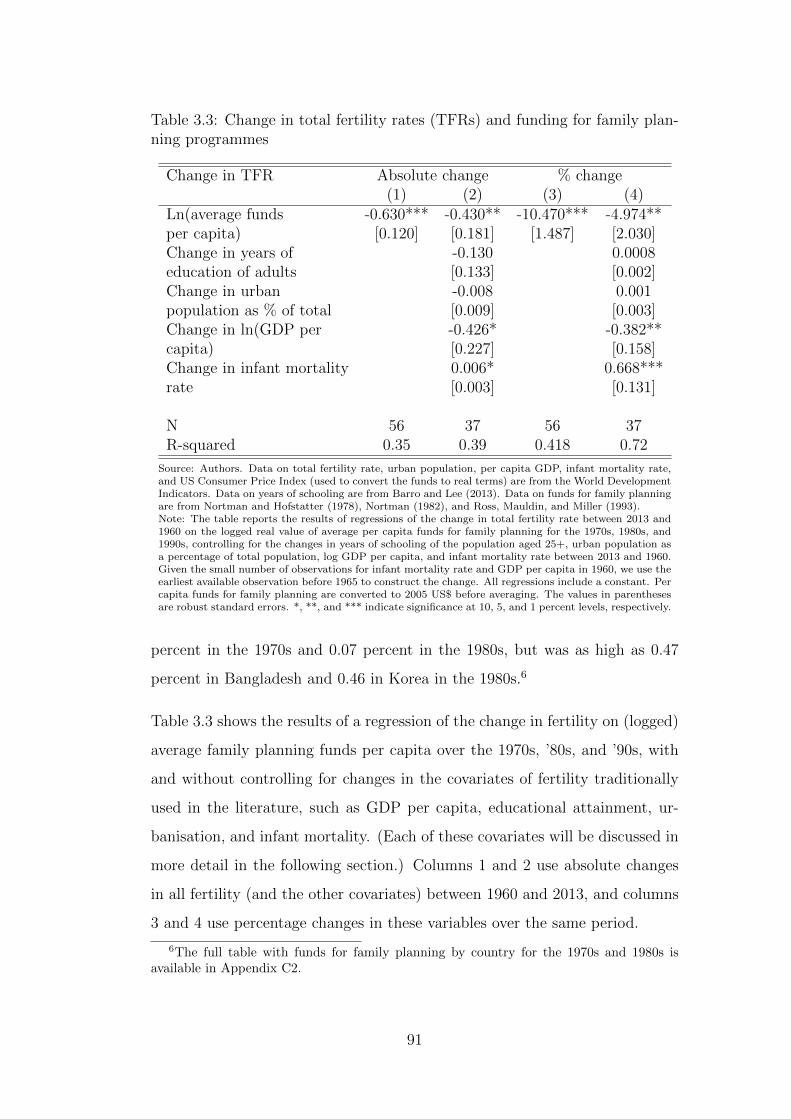
Table 3.3: Change in total fertility rates (TFRs) and funding for family plan-ning programmes
Change in TFR Absolute change % change(1) (2) (3) (4)
Ln(average funds -0.630*** -0.430** -10.470*** -4.974**per capita) [0.120] [0.181] [1.487] [2.030]Change in years of -0.130 0.0008education of adults [0.133] [0.002]Change in urban -0.008 0.001population as % of total [0.009] [0.003]Change in ln(GDP per -0.426* -0.382**capita) [0.227] [0.158]Change in infant mortality 0.006* 0.668***rate [0.003] [0.131]
N 56 37 56 37R-squared 0.35 0.39 0.418 0.72
Source: Authors. Data on total fertility rate, urban population, per capita GDP, infant mortality rate,and US Consumer Price Index (used to convert the funds to real terms) are from the World DevelopmentIndicators. Data on years of schooling are from Barro and Lee (2013). Data on funds for family planningare from Nortman and Hofstatter (1978), Nortman (1982), and Ross, Mauldin, and Miller (1993).Note: The table reports the results of regressions of the change in total fertility rate between 2013 and1960 on the logged real value of average per capita funds for family planning for the 1970s, 1980s, and1990s, controlling for the changes in years of schooling of the population aged 25+, urban population asa percentage of total population, log GDP per capita, and infant mortality rate between 2013 and 1960.Given the small number of observations for infant mortality rate and GDP per capita in 1960, we use theearliest available observation before 1965 to construct the change. All regressions include a constant. Percapita funds for family planning are converted to 2005 US$ before averaging. The values in parenthesesare robust standard errors. *, **, and *** indicate significance at 10, 5, and 1 percent levels, respectively.
percent in the 1970s and 0.07 percent in the 1980s, but was as high as 0.47
percent in Bangladesh and 0.46 in Korea in the 1980s.6
Table 3.3 shows the results of a regression of the change in fertility on (logged)
average family planning funds per capita over the 1970s, ’80s, and ’90s, with
and without controlling for changes in the covariates of fertility traditionally
used in the literature, such as GDP per capita, educational attainment, ur-
banisation, and infant mortality. (Each of these covariates will be discussed in
more detail in the following section.) Columns 1 and 2 use absolute changes
in all fertility (and the other covariates) between 1960 and 2013, and columns
3 and 4 use percentage changes in these variables over the same period.
6The full table with funds for family planning by country for the 1970s and 1980s isavailable in Appendix C2.
91

Despite the small number of observations available once the controls are in-
cluded, the negative relationship between changes in total fertility rate and
funds for family planning remains significant, indicating that the countries
with more funding for family planning experienced greater reductions in fertil-
ity rates, even after controlling for the changes in income, urbanisation, infant
mortality, and years of schooling of the adult population. (Controlling for
years of schooling of adult women instead of adult population leads to simi-
lar results.) Quantitatively, the results indicate that a 1 percent increase in
funding per capita is associated with a 5 percent reduction in the total fertility
rate.
We do not include changes in female labour force participation rates in this
regression because the cross-country data for this variable begins only in 1980.
However, we replicate the exercise focusing on changes between 1980 and 2013
for all variables and find that the results hardly change, with no significant
correlation between changes in female labour force participation and the fertil-
ity decline. We also carry out the exercise separately for government funding
and private funding for family planning per capita, and find that government
spending has a significant, positive correlation with the fertility decline whereas
private spending does not appear to be significant (see Appendix C3 and C4
for the full set of results).
Our third exercise uses the family planning programme effort index published
by Ross and Stover (2001) as an alternative measure of programme inputs. The
regional averages of the index indicate that East Asia and South Asia have,
in general, had the strongest family planning programmes over time. Latin
America, North Africa, and the Middle East seem to have caught up on pro-
gramme effort over the three decades, but the greatest gain appears to have
been in Sub-Saharan Africa, which was the latest to adopt family planning
programmes, in 1989–1999.7 We use these data to examine the relationship
between the observed change in fertility over the 1960–2013 period and the
7For more details on regional average program effort scores by year, see Appendix C5.
92

Table 3.4: Change in total fertility rates (TFRs) and family planning pro-gramme effort
Change in TFR Absolute change % change(1) (2) (3) (4)
Average family planning -0.039*** -0.041*** -0.716*** -0.500***programme effort score [0.007] [0.014] [0.101] [0.166]Change in years of -0.124 0.003education of adults [0.115] [0.003]Change in urban -0.012 -0.0001population as % of total [0.008] [0.005]Change in ln(GDP 0.015 -0.108per capita) [0.198] [0.192]Change in infant mortality 0.002 0.549***rate [0.003] [0.142]
N 107 55 107 55R-squared 0.21 0.41 0.321 0.636
Source: Authors. Data on total fertility rate, urban population, per capita GDP, and infant mortality rateare from the World Development Indicators. Data on years of schooling are from Barro and Lee (2013).Data on family planning programme effort are from Ross and Stover (2001).Note: The table reports the results of regressions of the change in TFR between 2013 and 1960 on the av-erage family planning programme effort score over the 1970s, 1980s, and 1990s, controlling for the changein years of schooling of the population aged 25+, urban population as a percentage of total population,log GDP per capita, and infant mortality rate between 2013 and 1960. All regressions include a constant.Given the small number of observations for infant mortality rate and GDP per capita in 1960, we usethe earliest available observation before 1965 to construct the change. All regressions include a constant.The values in parentheses are robust standard errors. *, **, and *** indicate significance at 10, 5, and 1percent levels, respectively.
average programme effort score over the 1970s, ’80s, and ’90s, again control-
ling for the other covariates of fertility. Table 3.4 indicates a strong negative
relationship, with larger fertility declines in countries with higher programme
effort.
Next, we use the Demographic and Health Surveys (DHS) data on percentage
of women exposed to family planning messages through mass media to carry
out the same exercise as for family planning programme funds and programme
effort score. Table 3.5 shows these results. The context of this analysis is
slightly different from the two previous exercises because the data are based
on DHS surveys which were carried out predominantly in sub-Saharan African
countries (30 of the countries in the sample used in columns 1 and 3, and 15 of
the countries in the sample used in columns 2 and 4) starting from the early
1990s. Therefore, these results capture more recent efforts in family planning
93

Table 3.5: Change in total fertility rates (TFRs) and exposure to family plan-ning messages
Change in TFR Absolute change % change(1) (2) (3) (4)
% of women with exposure -0.038*** -0.050*** -0.602*** -0.449**to FP messages [0.007] [0.011] [0.090] [0.169]Change in years of 0.054 0.001education of adults [0.154] [0.002]Change in urban -0.035** -0.016population as % of total [0.016] [0.010]Change in ln(GDP per -0.529** -0.379*capita) [0.244] [0.197]Change in infant mortality 0.002 0.551***rate [0.005] [0.175]
N 57 30 57 30R-squared 0.301 0.567 0.347 0.631
Source: Authors. Data on total fertility rate, urban population, per capita GDP, and infant mortalityrate are from the World Development Indicators. Data on years of schooling are from Barro and Lee(2013). Data on exposure to family planning messages are from Demographic and Health Surveys fromvarious years.Note: The table reports the results of regressions of the change in total fertility rate between 2013 and1960 on the percentage of women exposed to family planning messages through mass media for the ear-liest year (before 2005) for which information is available for that country, controlling for the change be-tween 2013 and 1960 in years of schooling of the population aged 25+, urban population as a percentageof total population, log GDP per capita, and infant mortality rate. All regressions include a constant.Given the small number of observations for infant mortality rate and GDP per capita in 1960, we use theearliest available observation before 1965 to construct the change. The values in parentheses are robuststandard errors. *, **, and *** indicate significance at 10, 5, and 1 percent levels, respectively.
as seen in sub-Saharan Africa.
The regression results show a significant, negative association between the fer-
tility change and exposure to family planning messages after controlling for
other covariates. It therefore seems likely that the delay in the implementa-
tion of the family planning programmes in sub-Saharan Africa explains the
delayed decline in fertility in the region. Both in Table 3.4 and Table 3.5, the
coefficients corresponding to the policy measure change little when adding the
controls; this suggests that additional omitted variables are unlikely to make
a difference.8
8As an additional robustness check, in the Appendix we exploit variation in the startingyear of state-led family planning programmes in 31 countries to further explore the relation-ship between fertility decline and the establishment of these programmes. After controllingfor changes in covariates as well as shocks that might have affected fertility in all countriesin a given year, we find that the decline in fertility accelerated with their inception. Giventhe very small sample size, which comprises mainly the early adopters of family planning,
94

These exercises demonstrate a strong association between the establishment
and intensity of family planning programmes with the decline in fertility rates,
after adjusting for changes in per capita income, urbanisation, infant mor-
tality, female labour force participation, and educational attainment. Most
sub-Saharan African governments acknowledged rapid population growth as
a policy concern much later than developing countries elsewhere. Even after
the formulation of population control policies, commitment to family planning
lagged behind that of other regions leading most international agencies work-
ing in family planning to invest their resources in the more promising areas of
Asia and Latin America. The onset of the HIV/AIDS epidemic is also likely
to have weakened the emphasis on fertility control due to limited resources
being targeted towards addressing the epidemic as well as the emergence of a
pro-natalist response to the high mortality rates caused by the epidemic (Na-
tional Research Council Working Group on Factors Affecting Contraceptive
Use 1993). While almost all African countries now provide direct or indirect
support for family planning, their efforts have only recently caught up with the
rest of the world. Perhaps not surprisingly in light of the strong correlations,
the countries in sub-Saharan Africa tend to be the ones where fertility rates
still remain above the world’s average.
3.4 Considering other explanations for the de-
cline in fertility
A number of other socioeconomic factors have been suggested as possible
causes for the decline in fertility: urbanisation, greater investment in edu-
cation per child, rising female labour force participation, and lower infant
mortality (see Becker 1960, Becker and Barro 1988, Barro and Becker 1989,
and Manuelli and Sheshadri 2009). The regressions presented in the previous
we do not place too much weight on these results, but consider it to be further suggestiveevidence in favor of the importance of these programmes in accelerating the fertility decline.The results of this analysis are available in Appendix C6.
95

section indicate that, population-control policies are strongly associated with
the fertility decline, whereas some of the traditional covariates display a much
weaker association. Of course, these results are hardly conclusive, as disen-
tangling cause and effect in this area is quite difficult, an issue compounded
by the shortage of data and potential measurement error. In this section, we
provide further arguments for why these factors, while important, are unlikely
to overshadow the role of population-control policies in the fertility decline.
Urbanisation has been put forward as an explanation for the decline in fertility,
as rural areas have historically had much higher fertility rates than urban ones.
Arguably, in rural areas, children can be a significant input in agricultural pro-
duction. Moreover, despite the fact that parents can earn higher average wages
in urban areas, it can cost more to raise children there, as the costs of housing
and (typically compulsory) education are higher.9 The negative relationship
between urbanisation and fertility is illustrated in Figure 3.5, which plots the
proportion of population living in urban areas against the total fertility rate for
all countries in 1960 and in 2013. Although countries with less urbanisation
have higher fertility, it does not appear that the urbanisation process alone
can account for the sharp decline in fertility rates observed over the past five
decades. Rather, it appears that fertility rates fell rapidly in both urban and
rural areas.
Given the strong possibility that the cross-country data on urbanisation is
mis-measured, we explored this issue in more detail using the Demographic
and Health Survey (DHS) data from 57 countries which, through their iden-
tification of rural and urban areas, provide separate rural and urban fertility
rates. The decline in fertility can be decomposed into a within-area effect,
corresponding to the decline in fertility within either rural or urban areas, and
9Becker (1960) argues that urbanisation could explain the decline in fertility. The ideais that farmers have a comparative advantage in producing children and food, though thisadvantage is smaller for higher “quality” of childbearing. Caldwell (1976)’s net wealthflow theory also supports the view that wealth flows from children to parents in primitiveagricultural societies, whereas the direction of flows reverses as society modernises and costsof raising children go up.
96

Figure 3.5: Fertility and urbanisation
Source: Authors using data from the World Development Indicators database.Note: For a sample of 190 countries, the figure shows the scatter plot and fitted line (smoothed lowessrelationship, or locally weighted smoothing function) between fertility and urbanisation in 1960 and 2013.Urbanisation is measured as the proportion of the population living in urban areas.
a between-area effect (that is, the urbanisation effect), corresponding to the
decline in fertility rates due to the increase in the share of the population living
in (lower-fertility) urban areas rather than (higher-fertility) rural areas.10 Per-
haps surprisingly, the increased urbanisation (between-area effect) contributed
to only about 14 percent of the fertility decline. Most of the decline in fertility
is explained by the within-area effect. Moreover, the contribution of urban-
isation to the decline in fertility does not vary significantly with a country’s
fertility or urbanisation rates. This result suggests that while urbanisation
may be a small part of the decline in fertility rates, other forces have been at
work driving down fertility in both rural and urban areas around the world.
The decline in fertility is often discussed as being part of a shift away from the
quantity of children towards higher quality, as demonstrated by the increase
in education levels around the world. There is clearly a strong negative re-
10It should be noted that, because these surveys were carried out in different years andat different intervals in different countries, the period over which the changes are computedis not the same for every country. Details of the data and calculations are available inAppendix D.
97

lationship between fertility and education, but it is difficult to establish the
direction of causality between fertility and education given that they are both
endogenous outcomes of a household’s decision-making process. For example,
quantity – quality trade-offs are analysed in Galor and Weil (2000) and Galor
and Moav (2002), where technological growth, by raising the return to human
capital, can generate a demographic transition (see also Doepke 2004). The
link between fertility and education emerges not just because of a tradeoff
between quantity and quality (or education) of the children, but also because
educated parents choose to have fewer children, possibly because they attach
more value to quality in that tradeoff or they have a comparative advantage in
educating children (Moav 2005). Remarkably, fertility has fallen significantly
even in countries and rural areas where educational attainment still remains
low. For instance, Bangladesh, Morocco, Myanmar, and Nepal all recorded
fertility rates below 2.7, with percentage declines of over 60 percent from their
1960 levels, despite their populations having less than five years of schooling
on average in 2010. Table 3.6 presents the average fertility rate in 2010 and
fertility change (between 2013 and 1960) for countries grouped by the level
of education of the adult population in 2010. While fertility rates are clearly
declining in the years of schooling of the population, all but the lowest educa-
tion group display sizeable percentage declines in fertility. The countries with
less than three years of schooling in 2010 are nearly all in sub-Saharan Africa,
where the fertility remains very high.
The cross-country correlation between female labour force participation and
fertility indicates only a weak relationship, given the high female labour force
participation in European and North American countries as well as in sub-
Saharan African countries. (Data on female labour force participation rates
are obtained from ILOSTAT.) Furthermore, labour force participation rates
did not change much over the past few decades, other than in Latin America
and the Caribbean, where the female labour force participation rate rose from
34 percent in 1980 to 54 percent in 2013. For comparison, over the same period,
female labour force participation fell slightly in East Asia and the Pacific (from
98
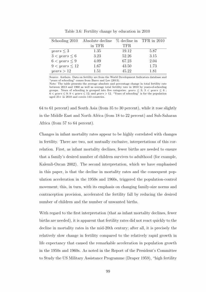
Table 3.6: Fertility change by education in 2010
Schooling 2010 Absolute decline % decline in TFR in 2010in TFR TFR
years ≤ 3 1.35 19.12 5.873 < years ≤ 6 3.23 52.26 3.156 < years ≤ 9 4.09 67.23 2.049 < years ≤ 12 1.67 43.50 1.73years > 12 1.51 45.22 1.81
Source: Authors. Data on fertility are from the World Development Indicators database and“years of schooling” comes from Barro and Lee (2013).Note: The table presents the average absolute and percentage change in total fertility ratebetween 2013 and 1960 as well as average total fertility rate in 2010 by years-of-schoolinggroups. Years of schooling is grouped into five categories: years ≤ 3; 3 < years ≤ 6 ;6 < years ≤ 9; 9 < years ≤ 12; and years > 12. “Years of schooling” is for the populationaged 25+ in 2010 and covers 143 countries.
64 to 61 percent) and South Asia (from 35 to 30 percent), while it rose slightly
in the Middle East and North Africa (from 18 to 22 percent) and Sub-Saharan
Africa (from 57 to 64 percent).
Changes in infant mortality rates appear to be highly correlated with changes
in fertility. There are two, not mutually exclusive, interpretations of this cor-
relation. First, as infant mortality declines, fewer births are needed to ensure
that a family’s desired number of children survives to adulthood (for example,
Kalemli-Ozcan 2002). The second interpretation, which we have emphasised
in this paper, is that the decline in mortality rates and the consequent pop-
ulation acceleration in the 1950s and 1960s, triggered the population-control
movement; this, in turn, with its emphasis on changing family-size norms and
contraception provision, accelerated the fertility fall by reducing the desired
number of children and the number of unwanted births.
With regard to the first interpretation (that as infant mortality declines, fewer
births are needed), it is apparent that fertility rates did not react quickly to the
decline in mortality rates in the mid-20th century; after all, it is precisely the
relatively slow change in fertility compared to the relatively rapid growth in
life expectancy that caused the remarkable acceleration in population growth
in the 1950s and 1960s. As noted in the Report of the President’s Committee
to Study the US Military Assistance Programme (Draper 1959), “high fertility
99

rates are normally part of deeply rooted cultural patterns and natural changes
occur only slowly.” This was also the view shared by demographers at the time
(Enke 1960; Davis 1967). Our regression analysis in the previous section has
attempted to gauge the two channels — the direct effect of infant mortality
declines, and population-control programmes — separately and both appeared
relevant. Another way to tease out the role played by population-control pro-
grammes as separate from the direct effect of infant mortality, is to study
trends in desired or ideal number of children and the share of unwanted preg-
nancies, which are two main targets of the population-control programmes.
In principle, according to the first interpretation, lower mortality rates should
only affect the number of births, not the ideal number of surviving children.11
Population-control programmes, however, focused on influencing the desired
number of children or family size.
The data from the Demographic and Health Surveys provide two measures
aimed at capturing fertility preferences: one is the “ideal number of children”
and the other is “wanted fertility rate.” The ideal number of children is ob-
tained as a response to the question: “If you could go back to the time you did
not have any children and could choose exactly the number of children to have
in your whole life, how many would that be?” The wanted fertility rate is con-
structed as the fertility rate that would be observed if all “unwanted” births
were eliminated; that is, births that raise the number of surviving children over
the stated desired number of children (Rutstein and Rojas 2006). We consider
the ideal or “desired” number of children as a measure of preference for surviv-
ing children: the number of children the woman would choose to have in her
whole life. In this context, fertility is directly affected by the desired number
of children, but can deviate from it for reasons that are unrelated to prefer-
ences, such as infant mortality or the availability of means to control fertility.
In particular, the wanted total fertility rate can exceed the desired number of
11Interestingly, the Barro and Becker (1989) framework predicts that, as mortality ratesfall, the ideal (or, in the jargon, “optimal”) number of surviving children actually increases,as the cost of raising children decreases. See Doepke (2005), who analyses different variantsof the Barro–Becker model yielding this prediction.
100

Table 3.7: Changes in wanted and unwanted fertility (as a percentage of changein total fertility rate)
Change as a % of change Overall Urban Ruralin TFRWanted fertility 75.35 63.48 82.26Ideal no. of children 57.97 56.08 51.92Other 17.38 7.41 30.35
Unwanted fertility 24.65 36.52 17.74
Note and Source: The table shows the change in wanted fertility rate andunwanted fertility rate (defined as the difference between total and wantedfertility rates) as a percentage of the change in total fertility rate using datafrom the Demographic and Health Surveys in 52 countries. The change inwanted fertility is further decomposed into the contribution of the changein the ideal number of children and a residual. Note that different coun-tries were surveyed in different years and at different intervals—the earliestavailable survey is from 1986 while the latest is from 2015.
children when women replace children who have died with additional births
to reach the desired number of surviving children (Bongaarts 2011). Table 3.7
uses data from Demographic and Health Surveys in 52 countries to present
the average change in wanted fertility rates as a percentage of the change in
total fertility rate over the period analysed (different countries were surveyed
in different years and at different time intervals, so the period over which the
changes are computed differ across countries). The change in wanted fertility
is further decomposed into the contribution of changes in the desired number
of children and a second (residual) component that captures other reasons,
which might include changes in infant mortality (under the heading “other”).
The data indicates that the fall in wanted fertility accounts for a significant
share of the fall in fertility, and that a large part of the fall in wanted fertility
can be accounted for by the decline in the number of desired children. The
pattern is observed in both rural and urban areas. The large role played by
the change in the desired or ideal number of children is supportive of the role
played by population programmes over and above the direct effect of lower
mortality rates.
The last row of Table 3.7 reports the change in unwanted fertility also as a
share of the change in total fertility rate. Unwanted fertility is defined as the
101

difference between total fertility rate and wanted fertility. Unwanted fertility
has also fallen in both urban and rural areas, pointing to improved ability to
control fertility given the wider availability of contraceptives. The decline in
unwanted fertility is relatively less important as a share of the change in overall
fertility. This, together with the large share accounted for by the decline in
the ideal number of children, is consistent with the introduction of additional
measures to promote a smaller family size as a result of the sluggish fertility
response to wider contraception provision.
3.5 Conclusion
The rapid decline in fertility rates in the past five decades cannot be accounted
for in a satisfactory way by economic growth, urbanisation, education levels,
or other socioeconomic variables. The timing and speed of the fertility de-
cline coincides with the growth of a neo-Malthusian global population-control
movement that designed and advocated a number of policy measures aimed
at lowering fertility rates across the world. The precise measures chosen by
different countries varied in nature and scope, depending on the individual
country’s socioeconomic context. But common to almost all programmes was
an enhanced provision of contraceptive methods and mass-media campaigns
to establish a new small-family norm.
The global convergence in fertility to near replacement fertility rates will even-
tually ensure a constant world population, although the rise in life expectancy
implies that it will take another few decades to reach a constant population
level. Projections by the UN Population division suggest that populations in
all regions except for Africa will stabilise by 2050. Including Africa, for which
the projections are more uncertain, world population is expected to stabilise
by 2100 at around 11.2 billion, with total fertility rates converging to 2 in all
regions (United Nations Population Division 2015). Concerns over possible
imbalances between resources and population will not disappear, but will be
102

mitigated as population growth flattens out. Insofar as the US experience can
offer guidance, the diffusion of contraception and the decline of fertility and
postponement of childbearing could increase female empowerment in develop-
ing countries through higher levels of investment in human capital (Goldin and
Katz 2002). To the extent that lower fertility rates are associated with higher
investment in human capital, the trends bode well for development and living
standards in the world’s poorest regions.
103

Appendices
Appendix B
In the paper we argue that the origins of the population control movement can
be traced to the West. In what follows, we reproduce extracts from historical
documents reflecting the preoccupation of intellectuals and policy makers in
the West with the high fertility levels.
John D. Rockefeller, Jr., 1934, in a letter to his father :
“In concluding, may I add one further statement in regard to my interest in
birth control. I have come pretty definitely to the conclusion that it is the field
in which I will be interested, for the present at least, to concentrate my own
giving, as I feel that it is so fundamental and underlying.” [Rockefeller 1934]
Report of the President’s Committee to Study the U.S. Military Assistance
Programme, 1959 :
“[T]hese high fertility rates are normally a part of deeply rooted cultural pat-
terns, and natural changes occur only slowly. In many countries, national
production is failing even to keep pace with population growth, and per capita
gross national product and food supplies are therefore decreasing rather than
increasing.
Government leaders in many of the less developed nations recognize that the
only hope for their people lies in accelerating the normal adjustment to the
rapidly declining mortality rate. Few countries have set up the necessary
programs, although broad acceptance has been found in those areas where
programs have been established.
The United States and the other more advanced countries can and should be
prepared to respond to requests for information and technical assistance in
connection with population growth. Such information will help to point up
the seriousness of the problem, and to encourage action in countries where
104

population pressures exist. Such information is also useful in defining the
areas in which initial efforts will be most effective. Recognizing an immediate
problem created by the rapid growth, the United States should also increase
its assistance to local programs relating to maternal and child welfare.
We Recommend: That, in order to meet more effectively the problems of
economic development, the United States (1) assist those countries with which
it is cooperating in economic aid programs, on request, in the formulation of
their plans designed to deal with the problem of rapid population growth, (2)
increase its assistance to local programs relating to maternal and child welfare
in recognition of the immediate problem created by rapid population growth,
and (3) strongly support studies and appropriate research as a part of its own
Mutual Security Program, within the United Nations and elsewhere, leading
to the availability of relevant information in a form most useful to individual
countries in the formulation of practical programs to meet the serious challenge
posed by rapidly expanding populations.” [Draper 1959, p 96-97]
John D. Rockefeller Jr. at the National Conference on the Population Crisis
1960 :
“In May 1960 at a National Conference on the Population Crisis co-sponsored
by the Dallas Council on World Affairs and Newsweek magazine, John D.
Rockefeller 3rd made a plea that was to be repeated many times in the decade
ahead: The problems of population are so great, so important, so ramified
and so immediate that only government, supported and inspired by private
initiative, can attack them on the scale required. It is for the citizens to
convince their political leaders of the need for imaginative and courageous
action-action which may sometimes mean political and economic opposition.”
[Piotrow 1973, p 49]
Enke (1960) based on discussions with senior officials and Prime Minister of
the Indian government :
“The willingness versus ability of adults to limit births has long been a matter
of controversy. A cheap and available contraceptive pill will not be the answer
105

in Asia unless couples wish to avoid pregnancies. . . In the ”extended” or three
generation households of Asia, which still predominate in rural areas, children
are not a liability to their parents during their infancy. And they are a real
asset in later life to their procreators.
It is not enough for governments in these countries to support clinics that
provide contraceptive information. It is not practical to tax extra children.
Instead, governments must offer some strong and positive inducement to cou-
ples to limit births. Money might be such an incentive if paid in large enough
amounts. Or other costly benefits, such as the education and support of par-
ents’ existing children, might be offered. [Enke 1960, p 343]
. . . In countries that are already overpopulated, and have crude population
increases of 2 percent a year, there may not be time to wait for uncertain
birth reductions following urbanization, emancipation of women, and a delayed
recognition that falling death rates have reduced the number of infants a couple
must have to obtain a given size family of grown children.
The knowledge and availability of contraceptives can be increased by govern-
ment action. But the ability rather than the willingness to limit family size is
affected thereby. Even a contraceptive pill is no panacea for the same reason.
It may benefit ”emerging” urban parents but not untutored rural peasants.
And, even if the pill cost only 10 cents, the total resource cost over the fer-
tile period of a woman’s life would exceed $100. So money payments to men
and women to constrain family size–in the ways described here–may be far
more effective a limitation and much cheaper in resources. Schemes of this
kind may do more for suffering humanity than successful medical research on
contraceptives.” [p 348]
Davis (1967) on the effectiveness of family planning programmes :
“By sanctifying the doctrine that each woman should have the number of
children she wants, and by assuming that if she has only that number this
will automatically curb population growth to the necessary degree, the leaders
106

of current policies escape the necessity of asking why women desire so many
children and how this desire can be influenced . . . Instead they claim that sat-
isfactory motivation is shown by the popular desire (shown by opinion surveys
in all countries) to have the means of family limitation, and that therefore the
problem is one of inventing and distributing the best possible contraceptive
devices. Overlooked is the fact that a desire for availability of contraceptives
is compatible with high fertility . . . We thus see that the inadequacy of current
population policies with respect to motivation is inherent in their overwhelm-
ingly family planning character. [Davis 1967, p 733-734]
. . . If excessive population growth is to be prevented, the obvious requirement
is somehow to impose restraints on the family. . . Population-control policy
can de-emphasize the family in two ways: (i) by keeping present controls over
illegitimate childbirth yet making the most of factors that lead people to post-
pone or avoid marriage and (ii) by instituting conditions that motivate those
who do marry to their families small. [p 737]
. . . In any deliberate effort to control the birth rate along these lines, a gov-
ernment has two powerful instruments – its command over economic planning
and its authority (real or potential) over education. The first determines (as
far as policy can) the economic conditions and circumstances affecting the lives
of all citizens; the second provides the knowledge and attitudes necessary to
implement the plans. The economic system largely determines who shall work,
what can be bought, what rearing children will cost, how much individuals can
spend. The schools define family roles and develop vocational and recreational
interests; they could, if it were desired, redefine the sex roles, develop inter-
ests that transcend the home, and transmit realistic (as opposed to moralistic)
knowledge concerning marriage, sexual behaviour, and population problems.
When the problem is viewed in this light, it is clear that the ministries of
economics and education, not the ministry of health, should be the source of
population policy.” [p 738]
John D. Rockefeller Jr. in a speech at the Population Tribune in Bucharest,
107

1974 :
“It turns out that women who avail themselves of family planning are chiefly
those who already have had many children. Over the 40-year span I have
referred to, the population of the world has increased by 86 percent, from
2.1 billion to 3.9 billion. And the absolute number of people in poverty has
continued to grow. Clearly, the programs that have been undertaken have
proved inadequate when compared to the magnitude of the problems facing
us. [Rockefeller 1978, p 511]
. . . [R]apid population growth is only one among many problems facing most
countries, it is a multiplier and intensifier of other problems. . . . [R]educing
population growth is not an alternative to development, but an essential part
of it for most countries.” [p 512]
National Security Study Memorandum 200 (The Kissinger Report), 1974 :
“High birth rates appear to stem primarily from: a. inadequate information
about and availability of means of fertility control; b. inadequate motivation
for reduced numbers of children combined with motivation for many children
resulting from still high infant and child mortality and need for support in old
age; and c. the slowness of change in family preferences in response to changes
in environment.
. . . We cannot wait for overall modernization and development to produce
lower fertility rates naturally since this will undoubtedly take many decades
in most developing countries, during which time rapid population growth will
tend to slow development and widen even more the gap between rich and poor.
[National Security Council 1974, p 6-7]
. . . The political consequences of current population factors in the LDCs -
rapid growth, internal migration, high percentages of young people, slow im-
provement in living standards, urban concentrations, and pressures for foreign
migration — are damaging to the internal stability and international relations
of countries in whose advancement the U.S. is interested, thus creating polit-
108

ical or even national security problems for the U.S. In a broader sense, there
is a major risk of severe damage to world economic, political, and ecological
systems and, as these systems begin to fail, to our humanitarian values. [p 8]
. . . While specific goals in this area are difficult to state, our aim should be for
the world to achieve a replacement level of fertility, (a two-child family on the
average), by about the year 2000. [p 9]
. . . The World Population Plan of Action is not self-enforcing and will require
vigorous efforts by interested countries, U.N. agencies and other international
bodies to make it effective. U.S. leadership is essential. The strategy must
include the following elements and actions:
a. Concentration on key countries. Assistance for population moderation
should give primary emphasis to the largest and fastest growing develop-
ing countries where there is special U.S. political and strategic interest.
Those countries are: India, Bangladesh, Pakistan, Nigeria, Mexico, In-
donesia, Brazil, the Philippines, Thailand, Egypt, Turkey, Ethiopia and
Columbia. Together, they account for 47 percent of the world’s cur-
rent population increase. (It should be recognized that at present AID
bilateral assistance to some of these countries may not be acceptable.)
Bilateral assistance, to the extent that funds are available, will be given
to other countries, considering such factors as population growth, need
for external assistance, long-term U.S. interests and willingness to engage
in self-help. Multilateral programs must necessarily have a wider cover-
age and the bilateral programs of other national donors will be shaped
to their particular interests. At the same time, the U.S. will look to the
multilateral agencies, especially the U.N. Fund for Population Activities
which already has projects in over 80 countries to increase population
assistance on a broader basis with increased U.S. contributions. This is
desirable in terms of U.S. interests and necessary in political terms in
the United Nations. But progress nevertheless, must be made in the key
109

13 and our limited resources should give major emphasis to them.
b. Integration of population factors and population programs into coun-
try development planning. As called for the world Population Plan of
Action, developing countries and those aiding them should specifically
take population factors into account in national planning and include
population programs in such plans.
c. Increased assistance for family planning services, information and tech-
nology. This is a vital aspect of any world population program. 1) Family
planning information and materials based on present technology should
be made fully available as rapidly as possible to the 85 % of the popula-
tions in key LDCs not now reached, essentially rural poor who have the
highest fertility.
d. Fundamental and developmental research should be expanded, aimed at
simple, low-cost, effective, safe, long-lasting and acceptable methods of
fertility control. Support by all federal agencies for biomedical research
in this field should be increased by $60 million annually.
e. Creating conditions conducive to fertility decline. For its own merits and
consistent with the recommendations of the World Population Plan of
Action, priority should be given in the general aid program to selective
development policies in sectors offering the greatest promise of increased
motivation for smaller family size. In many cases pilot programs and
experimental research will be needed as guidance for later efforts on a
larger scale. The preferential sectors include:. . .
– Developing alternatives to children as a source of old age security;
– Education of new generations on the desirability of smaller families. [p
10-11]
. . . The U.S. should encourage LDC leaders to take the lead in advancing family
planning and population stabilization both within multilateral organizations
and through bilateral contacts with other LDCs. This will require that the
110

President and the Secretary of State treat the subject of population growth
control as a matter of paramount importance and address it specifically in
their regular contacts with leaders of other governments, particularly LDCs.”
[p 12]
111

Appendix C
1 Features of early family planning programmes
Strategy Method of implementation Description
Increasing access to contraceptivesMinistry of Health clinics or hospital-
based facilities
All countries with a state-led family planning programme as well as coun-
tries where the state allowed private institutions to use state infrastructure
provided family planning services in clinics and hospitals.
Main examples: Mexico, Brazil, Uruguay, Kenya.
Post-partum family planning in ma-
jor hospitals
Women counselled on birth spacing and contraceptive methods soon after
delivery. Limited in scope as most deliveries did not take place in hospitals
in most developing countries at the time
Main examples: Iran, Sri Lanka, Colombia, Tunisia, Jamaica, Hong Kong,
Thailand, Malaysia, India, Ghana.
Pairing family planning with mater-
nal and child health services
While this was usually done in order to make use of existing medical
infrastructure, particularly in rural areas, it was also carried out in coun-
tries that wished to maintain a low profile for their programmes (e.g.,
Guatemala).
Main examples: Iran, Chile, Colombia, Korea, Singapore, Thailand,
Malaysia (rural areas), Philippines, Pakistan, Sri Lanka, Nepal, Brazil,
Honduras, Botswana, Guatemala.
Continued on next page
112

Continued from previous page
Strategy Method of implementation Description
Trained fieldworkers to reach remote,
rural areas
Midwives and/or community workers were trained to deliver and in some
cases prescribe or administer contraceptive methods.
Main examples: Egypt, Morocco, Korea, Hong Kong, Taiwan, Singapore,
Indonesia, Philippines, India, Pakistan and Bangladesh, Sri Lanka, Kenya,
Costa Rica, Colombia, Mexico, Iran, Nepal.
Mobile clinics and family planning
camps
Mobile clinics generally visited rural clinics, schools and government of-
fices on a regular basis. The team usually consisted of one person to
provide education and information and another to provide the medical
services.
Main examples: Iran, Hong Kong, Singapore, Malaysia, Nepal, Honduras,
Tunisia, Turkey, South Korea, India.
In India and Nepal, large scale vasectomy camps were set up temporarily
in primary health centers to perform sterilisations and insert IUDs
Contraceptive provision through in-
tegrated rural development pro-
grammes
Rural development projects (including education, sanitation and agricul-
tural projects) expanded to include a family planning component, usually
in the form of programme officers advocating and providing contraception
to target population alongside their usual activities.
Main examples: Philippines, Ghana, Iran, Turkey, Egypt.
Continued on next page
113

Continued from previous page
Strategy Method of implementation Description
Employment based family planning
programmesa
Contraceptive distribution, educational and promotional activities under-
taken by employers or labour unions usually working in collaboration with
a Family Planning Association or the government.
Main examples: Tata Iron and Steel Company in India, the military in
South Korea and Ecuador, Philippine Appliance Corporation, Misr Spin-
ning and Weaving Company in Egypt, Coffee Grower’s Association in
Colombia, as well as employers in Kenya, Thailand, China, Bangladesh,
Malaysia and Sri Lanka, labour unions in Turkey (TURK-IS) and Indone-
sia (Textile and Garment Labour Union).
Later (starting in the 1980s) Latin America and the Caribbean (where
most workers and their families are offered health care through the na-
tional social security system) extended their social security systems to
include family planning. Main examples in Latin America: Mexico, Peru
and Brazil.
Enabling private sector and NGO in-
volvement
In most countries, family planning programmes were originally piloted by
private family planning associations which were later supported (through
provision of state sector facilities and technical support) or taken over by
the state. These associations continue to play a role in service provision
and public education in many countries.
Continued on next page
114

Continued from previous page
Strategy Method of implementation Description
Main examples: Family Planning Associations in Chile (APROFA),
Colombia (PROFAMILIA), Guatemala (APROFAM), Jamaica (JFPA),
Costa Rica, Honduras, Mexico, Brazil and Uruguay continue to be lead-
ers in family planning activities alongside state programmes.
In Egypt, Iran, Tunisia, Morocco, Turkey, South Korea, Singapore, Hong
Kong, Taiwan, Indonesia, India, Pakistan, Bangladesh, Sri Lanka, Nepal,
Ghana, Kenya Zimbabwe, Botswana and Mauritius family planning asso-
ciations laid the foundations for large scale national programmes.
Subsidised contraceptive provision
and incentives for contraceptive us-
age
This included state subsidisation of private sector sale of contraceptives
(social marketing), provision of contraceptives at no cost, and provision
of incentives for the use of contraceptives.
Main examples: Social marketing programmes in Bangladesh, Pakistan,
India, Iran, Philippines, Honduras, Colombia, Mexico, Zimbabwe, Ghana,
Mauritius, Taiwan.
Certain family planning methods were provided free of charge in Jamaica,
Iran, Turkey, Malaysia, Sri Lanka, Morocco and China.
Patients, providers and/or fieldworkers bringing in the patient for sterilisa-
tions and IUD insertions compensated for travel and time in Bangladesh,
Nepal, India, Sri Lanka, South Korea.
Continued on next page
115

Continued from previous page
Strategy Method of implementation Description
Educating public on population is-
sues and contraceptive use
Interpersonal communication with
fieldworkers and community based
education
In addition to clinic based counselling, many programmes employed field-
workers to provide information about family planning at family planning
clinics and child health centres, on a door to door basis and even at mar-
riage and birth registries (Hong Kong).
Main examples: Egypt, Chile, Korea, Hong Kong, Taiwan, Indonesia,
Philippines, Pakistan, Bangladesh, Sri Lanka, Kenya, Iran, Singapore.
In Singapore, lectures and seminars on family planning were organised for
newlyweds, community leaders, teachers and school principals.
Print media such as posters, leaflets
etc.
Posters, leaflets, newspaper advertisements and magazine articles were
used to disseminate information about the benefits of contraceptive use,
technical information about specific contraceptive methods, nearest family
planning clinics, as well as to create awareness about the benefits of having
smaller families.
Main examples: Turkey, Korea, Singapore, India, Kenya, Egypt, Iran,
Mauritius, Hong Kong, Indonesia.
Electronic mass media including ra-
dio, film and television (particularly
important for reaching non-literate
population)b
Information on contraceptive use and population related issues was pro-
vided through spot announcements, interviews, news broadcasts, lectures,
drama, advertisements and even music. Most early programmes focused
on radio, later branching out into TV.
Continued on next page
116
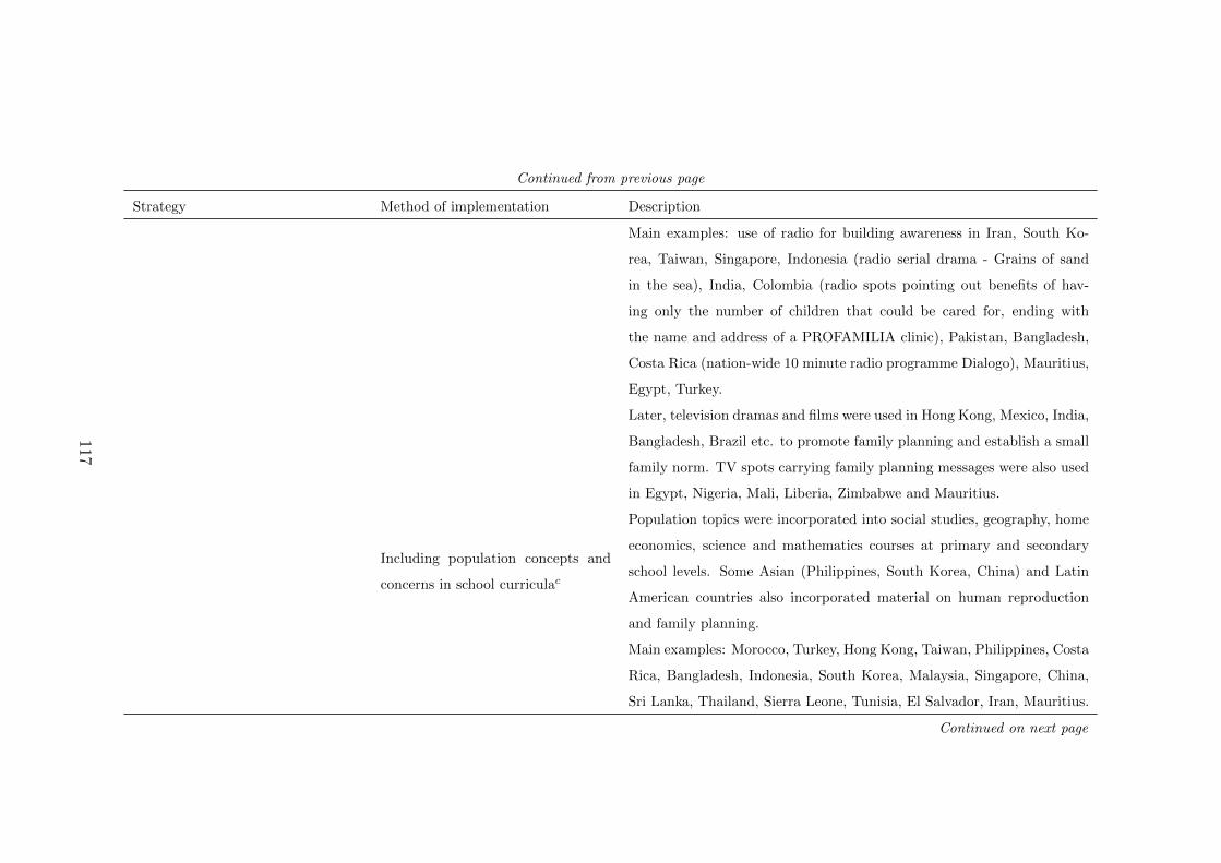
Continued from previous page
Strategy Method of implementation Description
Main examples: use of radio for building awareness in Iran, South Ko-
rea, Taiwan, Singapore, Indonesia (radio serial drama - Grains of sand
in the sea), India, Colombia (radio spots pointing out benefits of hav-
ing only the number of children that could be cared for, ending with
the name and address of a PROFAMILIA clinic), Pakistan, Bangladesh,
Costa Rica (nation-wide 10 minute radio programme Dialogo), Mauritius,
Egypt, Turkey.
Later, television dramas and films were used in Hong Kong, Mexico, India,
Bangladesh, Brazil etc. to promote family planning and establish a small
family norm. TV spots carrying family planning messages were also used
in Egypt, Nigeria, Mali, Liberia, Zimbabwe and Mauritius.
Including population concepts and
concerns in school curriculac
Population topics were incorporated into social studies, geography, home
economics, science and mathematics courses at primary and secondary
school levels. Some Asian (Philippines, South Korea, China) and Latin
American countries also incorporated material on human reproduction
and family planning.
Main examples: Morocco, Turkey, Hong Kong, Taiwan, Philippines, Costa
Rica, Bangladesh, Indonesia, South Korea, Malaysia, Singapore, China,
Sri Lanka, Thailand, Sierra Leone, Tunisia, El Salvador, Iran, Mauritius.
Continued on next page
117

Continued from previous page
Strategy Method of implementation Description
Other policies to encourage having
fewer childrenIncreasing the legal age of marriage Legal age of marriage increased in order to delay childbearing.
Main examples: Tunisia, India, China.
Incentives for having smaller familiesThese include explicit policies to discourage couples from having too many
children.
Main examples: Limiting government family allowances to the first four
children in Tunisia, number of children for which tax exemptions are
claimed cut to four and restricting paid maternity leave to four children in
Philippines, and restricting maternity leave to the first two children born,
restricting income tax relief to the first three children, and giving priority
for the allocation of public apartments for families with fewer children
among other policies in Singapore.
Notes: The table summarises key features of early family planning programmes around the world. Information on programmes in Egypt (Robinson and El-Zanaty 2007), Iran (Moore2007), Tunisia (Brown 2007b), Morocco (Brown 2007a), Turkey (Akin 2007), Chile (Sanhueza 2007), Colombia (Measham and Lopez-Escobar 2007), Guatemala (Santiso-Galvez andBertrand 2007), Jamaica (King 2007), South Korea (Kim and Ross 2007), Hong Kong (Fan 2007), Singapore (Teng 2007), Thailand (Rosenfield and Min 2007), Indonesia (Hull 2007),Malaysia (Tey 2007), Philippines (Herrin 2007), India (Harkavy and Roy 2007), Bangladesh and Pakistan (Robinson 2007), Sri Lanka (Wright 2007), Nepal (Tuladhar 2007), Ghana(Caldwell and Sai 2007) and Kenya (Heisel 2007) is from the compilation of case studies by Robinson and Ross (2007). Further information on the Latin American countries includingChile, Colombia and Guatemala is obtained from Shaffer (1968), Bertrand, Ward and Santiso-Galvez (2015) and the Cavenaghi (2009). Information on China (pre one-child policy)is obtained from Attane (2002) and Wang (2012). Information on Taiwan is obtained from Sun (2001). Information on Mauritius is from Hogan, Kennedy, Obetsebi-Lamptey andSawaya (1985) and the information on Botswana and Zimbabwe is taken from the report by the National Research Council Working Group on Factors Affecting Contraceptive Use(1993).a Information on this section is obtained from Rinehart, Blackburn and Moore (1987) b Information on this section is obtained from Gilluly and Moore (1986) and Church and Geller(1989) c Information on this section is obtained from Sherris and Quillin (1982)
118

2 Funds for family planning by country
Country
Total per Govt per Non-govt per Total funds
capita funds capita funds capita funds (% of GDP)
1970s 1980s 1970s 1980s 1970s 1980s 1970s 1980s
Asia
Afghanistan 2.56 0.00 2.56
Bangladesh 41.02 186.56 16.39 36.24 24.63 150.32 0.07 0.47
Hong Kong, China 54.65 66.00 26.74 48.42 27.91 17.57 0.01 0.00
India 68.42 99.55 64.10 89.67 4.32 9.88 0.08 0.16
Indonesia 74.75 101.37 39.52 71.38 35.23 29.99 0.09 0.11
Korea, Rep. 108.63 147.06 85.32 132.12 23.32 14.94 0.04 0.46
Malaysia 165.63 105.86 102.10 95.60 63.53 10.26 0.04 0.03
Mongolia 6.60 6.60 0.00
Nepal 28.06 35.94 15.67 27.93 12.40 8.02 0.07 0.12
Pakistan 76.01 41.58 32.21 18.07 43.79 23.51 0.13 0.07
Philippines 145.58 62.43 79.85 37.85 65.73 24.58 0.11 0.05
Singapore 134.12 97.74 132.62 97.38 1.50 0.36 0.01 0.01
Sri Lanka 16.11 16.68 11.76 4.92 0.02 0.02
Taiwan 50.88 89.44 46.52 89.35 4.36 0.10
Thailand 44.54 42.87 11.33 26.70 33.21 16.17 0.03 0.03
Vietnam 5.81
Latin America and Caribbean
Bolivia 13.20 0.96 12.25 0.01
Brazil 8.70 2.28 0.00 8.70
Colombia 59.18 47.40 23.70 23.70 0.02 0.02
Costa Rica 184.92 203.73 52.57 132.81 132.35 70.92 0.05 0.06
Dominican Rep. 91.42 43.28 48.15 0.04
El Salvador 300.66 324.76 237.06 235.47 63.60 89.29 0.15 0.22
Honduras 125.80 0.00 125.80 0.08
Nicaragua 204.57
Panama 59.59 14.29 45.30 0.01
Puerto Rico 897.43 390.17 507.26 0.09
Continued on next page
119

Continued from previous page
Country
Total per Govt per Non-govt per Total funds
capita funds capita funds capita funds (% of GDP)
1970s 1980s 1970s 1980s 1970s 1980s 1970s 1980s
Trinidad and Tobago 26.51
Venezuela 123.35 1.50
North Africa and Middle East
Egypt 16.33 1.81 11.96 14.51 0.01
Iran 248.01 243.34 0.07 4.67 0.05
Iraq 3.26 2.25 1.02 0.00
Jordan 61.82 21.45 40.37 0.02
Morocco 55.53 45.49 10.05 0.03
Tunisia 124.05 130.23 36.10 73.57 87.96 56.66 0.05 0.06
Turkey 23.03 23.58 21.81 20.51 1.22 3.06 0.01 0.01
Sub Saharan Africa
Botswana 15.40 7.48 7.93 0.01
Burkina Faso 23.93 6.70 17.23 0.05
Central African Rep. 35.21 16.93 18.28 0.05
Congo, Rep. 0.37
Ethiopia 6.66 0.02
Ghana 49.70 40.64 9.06 0.04
Guinea 15.24 0.71 14.53 0.02
Kenya 43.36 12.25 31.11 0.07
Liberia 48.34 0.08
Madagascar 3.78 1.46 2.32 0.01
Mauritania 29.51 0.76 28.75 0.04
Mauritius 356.05 385.87 180.29 244.30 175.76 141.58 0.11 0.12
Nigeria 9.39 0.02
Rwanda 55.90 29.90 25.99 0.10
Somalia 2.00 0.01
Tanzania 7.52 0.35 7.17
Uganda 5.63 0.01
Zambia 23.26 3.53 19.73 0.03
Continued on next page
120
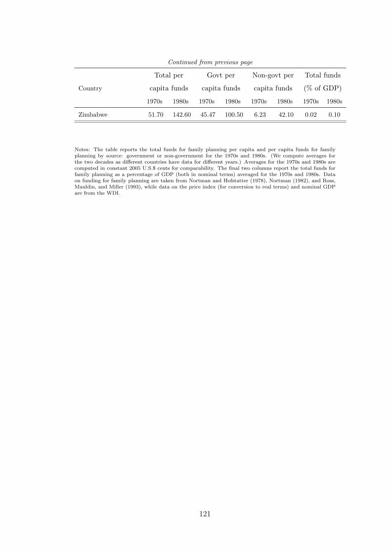
Continued from previous page
Country
Total per Govt per Non-govt per Total funds
capita funds capita funds capita funds (% of GDP)
1970s 1980s 1970s 1980s 1970s 1980s 1970s 1980s
Zimbabwe 51.70 142.60 45.47 100.50 6.23 42.10 0.02 0.10
Notes: The table reports the total funds for family planning per capita and per capita funds for familyplanning by source: government or non-government for the 1970s and 1980s. (We compute averages forthe two decades as different countries have data for different years.) Averages for the 1970s and 1980s arecomputed in constant 2005 U.S.$ cents for comparability. The final two columns report the total funds forfamily planning as a percentage of GDP (both in nominal terms) averaged for the 1970s and 1980s. Dataon funding for family planning are taken from Nortman and Hofstatter (1978), Nortman (1982), and Ross,Mauldin, and Miller (1993), while data on the price index (for conversion to real terms) and nominal GDPare from the WDI.
121
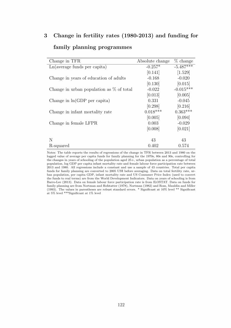
3 Change in fertility rates (1980-2013) and funding for
family planning programmes
Change in TFR Absolute change % changeLn(average funds per capita) -0.257* -5.487***
[0.141] [1.529]Change in years of education of adults -0.168 -0.020
[0.130] [0.015]Change in urban population as % of total -0.022 -0.015***
[0.013] [0.005]Change in ln(GDP per capita) 0.331 -0.045
[0.298] [0.216]Change in infant mortality rate 0.018*** 0.363***
[0.005] [0.094]Change in female LFPR 0.003 -0.029
[0.008] [0.021]
N 43 43R-squared 0.402 0.574
Notes: The table reports the results of regressions of the change in TFR between 2013 and 1980 on thelogged value of average per capita funds for family planning for the 1970s, 80s and 90s, controlling forthe changes in years of schooling of the population aged 25+, urban population as a percentage of totalpopulation, log GDP per capita infant mortality rate and female labour force participation rate between2013 and 1980. All regressions include a constant and use a sample of 43 countries. Total per capitafunds for family planning are converted to 2005 US$ before averaging. Data on total fertility rate, ur-ban population, per capita GDP, infant mortality rate and US Consumer Price Index (used to convertthe funds to real terms) are from the World Development Indicators. Data on years of schooling is fromBarro-Lee (2013). Data on female labour force participation rate is from ILOSTAT. Data on funds forfamily planning are from Nortman and Hofstatter (1978), Nortman (1982) and Ross, Mauldin and Miller(1993). The values in parentheses are robust standard errors. * Significant at 10% level ** Significantat 5% level ***Significant at 1% level
122
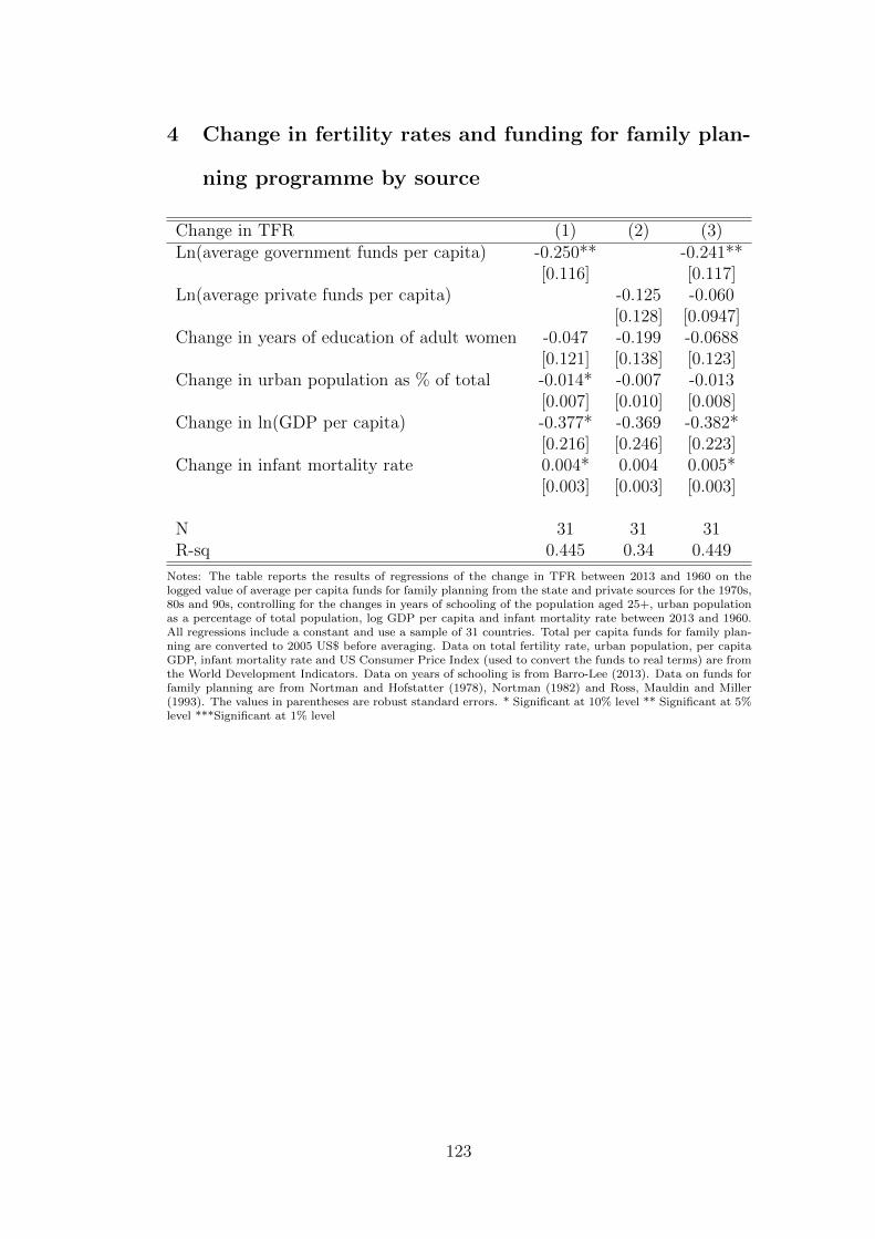
4 Change in fertility rates and funding for family plan-
ning programme by source
Change in TFR (1) (2) (3)Ln(average government funds per capita) -0.250** -0.241**
[0.116] [0.117]Ln(average private funds per capita) -0.125 -0.060
[0.128] [0.0947]Change in years of education of adult women -0.047 -0.199 -0.0688
[0.121] [0.138] [0.123]Change in urban population as % of total -0.014* -0.007 -0.013
[0.007] [0.010] [0.008]Change in ln(GDP per capita) -0.377* -0.369 -0.382*
[0.216] [0.246] [0.223]Change in infant mortality rate 0.004* 0.004 0.005*
[0.003] [0.003] [0.003]
N 31 31 31R-sq 0.445 0.34 0.449
Notes: The table reports the results of regressions of the change in TFR between 2013 and 1960 on thelogged value of average per capita funds for family planning from the state and private sources for the 1970s,80s and 90s, controlling for the changes in years of schooling of the population aged 25+, urban populationas a percentage of total population, log GDP per capita and infant mortality rate between 2013 and 1960.All regressions include a constant and use a sample of 31 countries. Total per capita funds for family plan-ning are converted to 2005 US$ before averaging. Data on total fertility rate, urban population, per capitaGDP, infant mortality rate and US Consumer Price Index (used to convert the funds to real terms) are fromthe World Development Indicators. Data on years of schooling is from Barro-Lee (2013). Data on funds forfamily planning are from Nortman and Hofstatter (1978), Nortman (1982) and Ross, Mauldin and Miller(1993). The values in parentheses are robust standard errors. * Significant at 10% level ** Significant at 5%level ***Significant at 1% level
123

5 Programme effort score by region
Region 1972 1982 1989 1994 1999Europe and Central Asia 20 27 46 42.2 53East Asia and the Pacific 39.4 46.1 52.5 55.7 58.5Latin America and the Caribbean 30.2 39 50.6 50.3 50North Africa and the Middle East 11.4 17.9 40.5 41.8 58.3South Asia 24.3 46.3 55.6 56.8 64.4Sub Saharan Africa 5 15.5 36.7 43.9 51.1Total 19.3 28.5 44.3 47.8 53.6
No. of countries 89 94 92 95 88
Notes: The table reports the average family planning programme effort score for each region. Theregional averages are calculated using data from Ross and Stover (2001).
124

6 Effect of state-led family planning programme imple-
mentation on fertility decline
∆TFRt (1) (2) (3)State programme -0.066**
[0.023]L1.State programme -0.059**
[0.020]L2. State programme -0.050*
[0.018]∆GDPt 0.009 0.005 0.003
[0.078] [0.077] [0.080]∆IMRt 0.001 0.002 0.002
[0.005] [0.005] [0.005]∆Urbant -0.022 -0.021 -0.021
[0.016] [0.016] [0.016]∆Edut 0.006 0.006 0.005
[0.011] [0.011] [0.011]
Total obs. (NT) 1574 1574 1553R-squared 0.191 0.187 0.177
Notes: The table reports the results of fixed effects regressions of the yearon year change in TFR on a dummy variable for establishment of state fam-ily planning programme (0 before establishment, 1 after), controlling for theyear on year change in the log of per capita GDP, infant mortality rate,urban population as a % of total population and years of schooling of thepopulation aged 25+. Columns (2) and (3) use 1 and 2 year lags of the pro-gramme dummy, respectively. All regressions are estimated using a sampleof 31 countries and include country and year fixed effects. Data on total fer-tility rate, urban population, per capita GDP, and infant mortality rate arefrom the World Development Indicators. Data on years of schooling is fromBarro-Lee (2013). Since years of schooling at available at 5-yearly intervalswe replace missing values with data from the closest year for which datais published. Data on family planning programme implementation datesare compiled using information from Robinson and Ross (2007), Cavenaghi(2009), Shaffer (1968), Bertrand et al (2015), Attane (2002), Hogan et al(1985) and National Research Council Working Group on Factors AffectingContraceptive Use (1993). The values in parentheses are robust standarderrors. * Significant at 10% level ** Significant at 5% level ***Significant at1% level
125

Appendix D
In formulas, the overall fertility rate equals the weighted average of urban and
rural fertility rates:
Ft = λr,tFr,t + λu,tFu,t
Where λr,t is the proportion of the country’s population living in rural areas
in period t, λu,t = 1 − λr,t, and Fr,t and Fu,t are the rural and urban fertility
rates at time t, respectively.
With some algebra, the change in overall fertility between time 0 and time
t can be exactly decomposed as:
∆Ft = Ft − F0 = (∆λr,tFr,t + ∆λu,tFu,t)︸ ︷︷ ︸Between (urbanisation) effect
+ (λr,t∆Fr,t + λu,t∆Fu,t)︸ ︷︷ ︸Within effect
where 0 and t correspond to the start and end of the period, respectively; and
the terms denoted with a bar are the time averages: xj = (xj,t + xj,0)/2, for
j = r, u;x = λ, F
The results of the decomposition exercise are presented in the table below.
Fertility rate decomposition by region
Country Change in Between Within First year Last year
fertility effect effect
Angola 0.5 108.82% -8.82% 2006 2011
Bangladesh -1.1 6.82% 93.18% 1993 2014
Benin -1.1 8.65% 91.35% 1996 2011
Bolivia -1.5 8.03% 91.97% 1989 2008
Brazil -0.9 18.32% 81.68% 1986 1996
Burkina Faso -1 17.41% 82.59% 1993 2014
Burundi -0.8 14.63% 85.37% 1987 2012
Cambodia -1.1 7.58% 92.42% 2000 2014
Continued on next page
126

Continued from previous page
Country Change in Between Within First year Last year
fertility effect effect
Cameroon -0.7 21.78% 78.22% 1991 2011
Colombia -1.1 21.19% 78.81% 1986 2010
Comoros -0.3 21.37% 78.63% 1996 2012
Congo, Dem. Rep. 0.3 40.30% 59.70% 2007 2013
Congo, Rep. 0.3 -96.59% 196.59% 2005 2011
Cote d’Ivoire -0.3 43.75% 56.25% 1994 2011
Dominican Republic -1.2 -11.64% 111.64% 1986 2013
Egypt, Arab Rep. -1 -31.42% 131.42% 1988 2014
Eritrea -1.3 16.86% 83.14% 1995 2002
Ethiopia -0.7 31.49% 68.51% 2000 2011
Gabon -0.1 200.00% -100.00% 2000 2012
Ghana -2.2 13.64% 86.36% 1988 2014
Guatemala -2.4 9.38% 90.62% 1987 2014
Guinea -0.4 -1.36% 101.36% 1999 2012
Guyana 0.3 27.78% 72.22% 2005 2009
Haiti -1.3 13.02% 86.98% 1994 2012
Honduras -0.4 20.83% 79.17% 2005 2011
India -0.7 4.52% 95.48% 1992 2005
Indonesia -0.5 15.00% 85.00% 1987 2012
Jordan -2.1 4.93% 95.07% 1990 2012
Kazakhstan -0.5 8.71% 91.29% 1995 1999
Kenya -3 22.70% 77.30% 1989 2015
Kyrgyz Republic 0.2 -56.87% 156.88% 1997 2012
Lesotho -0.2 97.16% 2.84% 2004 2014
Liberia -2 20.83% 79.17% 1986 2013
Madagascar -1.7 -18.15% 118.15% 1992 2013
Malawi -2.3 2.27% 97.73% 1992 2015
Mali -0.8 -4.40% 104.40% 1987 2015
Morocco -2.1 4.89% 95.11% 1987 2003
Mozambique 0.7 -38.10% 138.10% 1997 2011
Continued on next page
127

Continued from previous page
Country Change in Between Within First year Last year
fertility effect effect
Namibia -1.8 25.03% 74.97% 1992 2013
Nepal -2 4.76% 95.24% 1996 2011
Nicaragua -0.4 0.00% 100.00% 1998 2001
Niger 0.6 -15.24% 115.24% 1992 2012
Nigeria -1 11.28% 88.72% 1990 2015
Pakistan -1.1 4.85% 95.15% 1990 2012
Peru -1.5 9.17% 90.83% 1986 2012
Philippines -1.1 1.71% 98.29% 1993 2013
Rwanda -2 5.46% 94.54% 1992 2014
Senegal -1.4 21.92% 78.08% 1986 2014
Sierra Leone -0.2 14.32% 85.68% 2008 2013
Tanzania -1 17.94% 82.06% 1991 2015
Togo -1.6 10.31% 89.69% 1988 2013
Turkey -0.3 33.33% 66.67% 1993 2003
Uganda -1.7 17.44% 82.56% 1988 2014
Vietnam -0.4 -3.89% 103.89% 1997 2002
Yemen, Rep. -3.3 12.01% 87.99% 1991 2013
Zambia -1.2 -2.32% 102.32% 1992 2013
Zimbabwe -1.4 11.48% 88.52% 1988 2015
Notes: The table reports the overall decline in fertility, the percentage of the change dueto the between-area effect (urbanisation effect) and within-area-effect, and the years overwhich the overall change is calculated. Data on total and urban and rural fertility ratesare obtained from the Demographic and Health Surveys. Proportion of urban population iscalculated as λu,t =
Ft−Fr,t
Fu,t−Fr,t.
128

Chapter 4
The Large Fall in Global
Fertility: A Quantitative Model
4.1 Introduction
Most developing countries experienced remarkable declines in total fertility
rates (TFR) over the past few decades. The world’s average TFR declined
steadily during this period, falling from 5 children per woman in 1960 to 2.4
in 2015. This decline in fertility is not skewed by the experience of a few
countries. In 1960, more than half of the countries in the world experienced
fertility rates greater than 6. By 2015, the median TFR was 2.2 children per
woman. Interestingly, the rapid decline in fertility has taken place in countries
at widely different levels of development.
In the previous chapter, we have argued that while socioeconomic factors play
an important role in the worldwide fertility decline, the timing and speed of the
decline over the past five decades suggests that the population control policies
implemented in many developing countries over this period might have played
a significant role in accelerating the process. The design of population-control
programmes consisted of two main parts. The first was the diffusion of contra-
129

ceptive supply and information. The second was the implementation of public
campaigns aimed at reversing pro-natalist attitudes and establishing a new
small-family norm. We argued that the second strategy of employing public
campaigns to reduce desired levels of fertility was critical in complementing
contraceptive provision.
To analyse the rapid decline in fertility, we study a model of endogenous fertil-
ity and human capital accumulation, augmented to include a role for endoge-
nously evolving social norms on family size. In the model, individuals derive
utility from both the quantity and “quality” of children and dislike deviating
from the social norm on the number of children, where the norm is a weighted
average of the fertility of the previous generation and the replacement level of
fertility, which is close to two.1
Calibrating the model’s structural parameters and initial conditions to match
key moments in the data for developing countries in 1960, we use the model to
simulate the transition to the steady-state levels of fertility and human capi-
tal. While the baseline model with no role for norms is able to endogenously
generate a slight decline in fertility, we find that incorporating social norms
into the model generates a much larger decline.
We then simulate the effect of population-control policies on family-size norms
using information on funding for family-planning programmes. In particular,
we allow the weight placed on the fertility of the previous generation - family
size is greatly influenced by the family of origin - to decline with the intensity
of these programmes, given that the majority of these programmes advocated
having two children. We also consider several alternative mechanisms that
might explain the fertility decline, including the fall in infant and child mor-
tality and improvements in contraceptive technologies (the second component
of the population-control policies). The model allows us to gauge quantita-
tively the role played by these different channels - human capital accumulation,
1We follow the literature’s jargon, where “quality” relates to the level of human capitalof the individual.
130
declining infant mortality, improved control over fertility, and reductions in the
social norm on family size - in generating the fertility decline.
We find that the baseline model without norms generates a small decline in
fertility. The inclusion of endogenously evolving social norms on fertility can
generate a decline in fertility which is twice as large as the decline generated
by the baseline mode, but still not enough to replicate the large declines in the
data. We find that policies aimed at altering family-size norms significantly
accelerate and strengthen the decline in fertility that would have otherwise
gradually taken place as economies move to higher levels of human capital,
lower levels of infant mortality, and higher supplies of contraceptive technolo-
gies.
The rest of the paper is organized as follows. Section 4.2 describes the model
and Section 4.3 explains the calibration strategy. Section 4.4 presents the
main results of the paper and Section 4.5 studies various extensions. Section
4.6 presents concluding remarks.
4.2 The Model
This Section studies a simple quantitative model of endogenous human cap-
ital and fertility choice. The goal is to gauge the impact of human capital
accumulation and population-control policies on the rapid fall in fertility ex-
perienced by most developing countries in recent decades. The model builds
on the Barro-Becker framework of fertility choice, incorporating human capi-
tal investment (see Barro and Becker 1989; Galor and Weil, 2000; Galor and
Moav, 2002; Moav, 2005). We sequentially extend the analysis along many
dimensions. First and foremost, we augment the model by introducing social
norms on family size, which were a key target of population-control policies in
developing countries.
Our modelling of adherence to social norms borrows from the literature on
131

social distance and conformity (Jones 1984, Akerlof 1997) in that individuals
derive disutility from a function of the distance between their realised fertility
and the social norm.2
We define the social norm on fertility as a weighted average of the fertility
rate of the previous generation and the replacement level of fertility. The first
term draws from the sociology literature that discusses the importance of ref-
erence groups in forming fertility norms (e.g. Clay and Zuiches 1980). Norms
on family size are highly influenced by the family of origin.3 We choose the
replacement level as the second term in the average based on the observation
that most economies appear to be converging to a similar focal point for fertil-
ity, currently just about two children per woman. This endogenously evolving
norm naturally leads to a decline in fertility that is larger than that generated
in a model without social norms. In this baseline model, we assume house-
holds perfectly control fertility. We model the impact of the family planning
programmes and their mass communication strategies as an increase in the
weight placed on the replacement level of fertility, causing the social norm on
family size to shift downwards, accelerating the decline even more.
In further extensions of the model we also consider the role played by the
overall fall in mortality rates. In a setting in which there is child mortality
and uncertainty about how many children survive to adulthood, we find that
the decline in mortality alone is not sufficient to explain the fall in fertility
observed over the past few decades.4 The decline in mortality rates did seem
2We deviate from the existing work on the impact of social norms on fertility in howwe model social norms. Munshi and Myaux (2005), Palivos (2001) and Bhattacharya andChakraborty (2012) model norms as the outcome of strategic decisionmaking and interaction,We take a simpler specification that is more amenable to quantification and in line with theliterature on external habits or reference dependence.
3The impact of parental fertility on their children’s fertility is also explored in the de-mography literature, focusing on developed countries. For example, Thornton 1980, Murphy1999 and Kolk 2014.
4This point was previously made by Doepke (2005). Becker and Barro (1988)’s modelpredicts that when mortality rates decrease, the total fertility rate falls, but the numberof surviving children remains the same. In survey data, we observe a decline not only infertility rates, but also in the desired number of children. Kalemli-Ozcan (2002) introducesa precautionary motive to have children; in that context, a decline in mortality reduces boththe fertility rate and the number of (desired) surviving children.
132

to have played an important role in triggering population-control policies, but
it is unlikely to have fueled the fast fall in fertility through individual or de-
centralised responses, without the policy intervention. A second extension
considers the case in which households cannot directly control fertility rates
(contraception technologies are either not available or imperfect) and the role
played by increased access to contraception (the second main component of
population-control policies).
We do not explicitly model the possibility that children provide their parents
with transfers in their old age, but our modelling choices can be recast in
those terms, as parents care about their children’s future earning capacity.5
In what follows, we describe the model in more detail, specifying technologies
and preferences.
4.2.1 Model setup
We consider an overlapping generation economy in which individuals live for
two periods: childhood and adulthood. In each period, the economy produces
a single consumption good using the productive capacity of the working adults
and a fixed factor as inputs, where the supply of the fixed factor is exogenous.
The human capital stock is determined by the fertility and educational choices
of individuals.
4.2.2 Technology
Production occurs according to a constant returns to scale production tech-
nology. Using the specification in Galor and Weil (2000), output at time t, Yt
is
Yt = ((H +Ht)Lt)ρ(AtX)1−ρ, 0 < ρ < 1 (4.1)
5There is a growing literature which addresses these inter-generational transfers explicitly(see for example Boldrin and Jones 2002, Coeurdacier, Guibaud and Jin 2014, Choukhmane,Coeurdacier and Jin 2014).
133

where H + Ht is the productive capacity of a worker, Lt is the working age
population, X is the fixed factor and At is the technology at time t, with AtX
referring to “effective resources”. The term H is a physical labour endow-
ment all individuals are born with and Ht is human capital produced with
investments in schooling.
Output per worker at time t, yt, is
yt = ((H +Ht))ρx1−ρ
t , (4.2)
where xt = AtX/Lt is the effective resources per worker at time t.
As in Galor and Weil (2000), we assume that the return to the fixed factor is
zero. This assumption helps to keep the model simple so that the only source
of earnings for households is labour income, which is true for many households
in developing countries. X can then be interpreted as some productive public
good which does not yield private returns to the citizens. (Galor and Weil
(2000)’s interpretation is that there are no property rights over this resource
in the country). Alternatively, as in Cespedes and Velasco (2012), one can
think of X as being owned by a small group of “elite” individuals, who spend
all the returns from X abroad (and whose behaviour we do not consider in our
model).
The return to productive labour, wt, is then given by its average product:
wt =
(xt
(H +Ht)
)1−ρ
(4.3)
4.2.3 Households
Each household has a single decision maker, the working adult. Individuals
within a generation are identical. Children consume a fraction of their parents’
time. Working adults supply labour inelastically, decide on their consumption,
the number of children, and their education in period t.
134

Parents are motivated by altruism towards their children but are conscious
of the social norm on the number of children that a family should have. As
such, while parents derive utility from their children (both the quantity and
the quality), they derive disutility from deviating from the social norm. The
utility function for a working age individual of generation t can be expressed
as:
Ut = u(Ct; nt; qt+1)− ϕg(nt, nt), (4.4)
where u is a standard utility function over three goods: Ct, denoting con-
sumption at time t, nt, which denotes the number of children, and qt+1,
which indicates the quality of children as measured by their future earning
potential. Following Galor and Weil (2000) and Moav (2005), we assume
qt+1 = wt+1(H + Ht+1), where wt+1 is the future wage per unit of productive
labour of a child, and H+Ht+1 is the productive capacity of a child. The factor
ϕ > 0 governs the disutility from deviating from the social norm and g(nt, nt)
is a function of the deviation of the chosen number of children, nt, from the
social norm on family size, nt, where g11(nt, nt) > 0 and g12(nt, nt) < 0. The
first condition implies that movements further away from the norm involve
heavier penalties while the second implies that the marginal cost of the ad-
ditional child is decreasing in the social norm. We model the social norm on
family size as a weighted average between the previous generation’s fertility,
nt−1 and the replacement level of fertility, n∗, so that nt can be expressed as:
nt = φn∗ + (1− φ)nt−1, 0 ≤ φ ≤ 1 (4.5)
The individual’s choice of desired number of children and optimal education
investment for each child is subject to a standard budget constraint. While
parental income is given by wt(H + Ht), we assume that a fixed fraction of
income, τ0, is spent on each child regardless of education while a discretionary
education cost for each child, τ1ht, which is increasing in the level of education,
ht, is chosen by the parents. The remaining income is spent on consumption.6
6It is also possible to interpret the constraint as a restriction on the total amount of time
135

The budget constraint at time t is therefore,
Ct = [1− (τ0 + τ1ht)nt]wt(H +Ht) (4.6)
Following Becker, Murphy, and Tamura (1990) and Ehrlich and Kim (2005),
we specify the human capital production function as:
Ht+1 = zt(H +Ht)ht, (4.7)
where H + Ht is the productive capacity of the parent, ht is the educational
investment (or schooling) in each child and zt is the human capital production
technology. This specification of productive capacity prevents perfect intergen-
erational transmission of human capital, allowing for positive levels of human
capital even for children whose parents have no schooling (Ht = 0).
4.2.4 Equilibrium
In a competitive equilibrium, agents and firms optimally solve their problems
and all markets clear. Let v = (H + Ht, nt−1). A competitive equilibrium
for this economy consists of a collection of policy functions for households
{Ct(v), nt(v), ht(v)}, and prices wt such that:
1. Policy functions Ct(v), nt(v), and ht(v) maximise
u(Ct;nt; qt+1)− ϕg(nt, nt)
subject to the budget constraint (4.6), human capital production function
(4.7) and (Ct, nt, ht) ≥ 0;
2. wt satisfies (4.3); and
available to work and have and raise children. In that case, τ0 would be the fraction of timethat has to be spent on raising a child regardless of the education level.
136
3. Markets clear such that:
Ct = [1− (τ0 + τ1ht)nt]yt
4.3 Calibration
In the policy experiments that we carry out, we examine the transition of
the economy from a given initial condition to a steady state level of fertility
and human capital investment. Our calibration strategy, therefore, involves
choosing structural parameters and initial conditions so that the outcomes of
the model in the first period match the appropriate moments for consumption,
income, fertility, education and population in developing countries in 1960.7
Since the economic agent in this model is an individual, the fertility rate in the
model is one half of the total fertility rates in the data. Similarly, we interpret
the units of investment in human capital per child, ht, as years of education.8
In addition, one period in the model corresponds to the length of a generation,
around 25 years.
The data on household consumption, per capita GDP, working age population
and fertility are obtained from the World Bank’s World Development Indica-
tors (WDI) dataset while the data on average years of education are taken from
the Barro-Lee educational attainment datasets (Barro and Lee 2010, Barro and
Lee 2015).
7We refer to all countries which were not classified as OECD countries prior to 1970 asdeveloping countries in the starting period. 1960 is the first year for which cross-countrydata on fertility, income, education and consumption are available.
8The data available is the average years of education of the adult population (aged 25and above). As such, the investment in education for children born in a given period isobserved in the data as the average years of education of the adult population in the nextperiod. I.e., if the length of a generation is 25 years, h1960 is given by the average years ofeducation of the adult population in 1985.
137
4.3.1 Technology
We set the productive labour share of income, ρ, to 0.66. Estimates of total
factor productivity in East Asian countries over the 1966-1990 period by Young
(1995) indicate that on average, annual TFP growth over the period ranged
from -0.003 in Singapore to 0.024 in Taiwan. As such, we will assume a constant
annual TFP growth rate of 0.018 which is compounded to obtain the TFP
growth rate between generations, gA.9 In addition, we assume that there is no
growth in the technology used in human capital production, zt.
4.3.2 Cost of childrearing
Household expenditure surveys report the fraction of household expenditure
spent on education. In our model, this fraction is represented by τ1ntht. This
ranges from 2.6 percent in India in 2007/08 to 5.5 percent in Singapore in
2012/13. However, the value for τ1, calculated using corresponding values for
nt and ht from the data, is much more uniform, around 0.3 percent.10 We
therefore set τ1 to 0.003. We then use the household budget constraint to back
out the value for τ0, given the initial levels of income, consumption, fertility
and education.
4.3.3 Preferences
We assume utility is additively log linear in consumption, the number of chil-
dren, the quality of children and social norms:
Ut = lnCt + α lnnt + θ ln[wt+1(H +Ht+1)]− ϕg(nt, nt), (4.8)
9Our specification of utility implies that the value of gA affects the simulations onlythrough the initial value for the human capital stock as wages do not have an effect onfertility or human capital investment decisions. Assuming gA = 0 barely changes the resultsof the quantitative exercise.
10See Appendix E1 for the full set of countries and expenditure statistics.
138

where α > 0 reflects preferences for children, θ > 0 for child quality.
As noted in Akerlof (1997), the use of the absolute value of the difference
between individual fertility and the social norm gives rise to multiple equilibria.
We use a more tractable functional form given by:
g(nt, nt) = (nt − nt)2,
where individuals derive disutility from deviating above as well as below the
social norm and deviations in either direction are penalised symmetrically. In
Section 4.5 we consider a different functional form which treats upward and
downward deviations asymmetrically and find that the results are very similar.
Given these preferences, the first order condition for nt is given by:
α
nt=
(τ0 + τ1ht)
1− (τ0 + τ1ht)nt+ 2ϕ(nt − nt) (4.9)
The FOC equates the marginal benefit of having children with the marginal
cost. The first term on the right hand side is the marginal cost in terms of
foregone consumption while the second term will be a cost if the additional
child pushes the total number of children over the social norm.
The first order condition for ht is
θzt(H +Ht)
(H +Ht+1)=
τ1nt(1− (τ0 + τ1ht)nt)
, (4.10)
where the right hand side is the marginal utility to the parent from giving her
child an additional unit of education and the left hand side is the marginal
cost in terms of foregone consumption.
Our specification of utility leaves us with three preference parameters (α, θ,
and ϕ) to be calibrated. We also require initial values for Ht and zt. We
start by calibrating a baseline model in which individuals do not care about
norms (ϕ = 0) and pin down α from the first order condition for nt, using
139

the cross-country macro data for developing countries for 1960. We use the
output growth in the economy to pin down H+Ht+1
H+Ht(which we will refer to as
gH , hereafter). Then, for given values of zt (which we choose to match the
empirical estimates of the returns to schooling) and H, we use the first order
condition for ht and the human capital production function to obtain values
for θ and H1, the level of human capital of parents in the initial period.11
4.3.4 Norms
We now use the first order condition for fertility from the full model (equation
4.9) to obtain a value for φ, for given values of ϕ and nt−1. We do not have
enough moments in the data to back out ϕ and, to the best of our knowledge,
there are no empirical measures of this parameter. Therefore, we set ϕ = 0.1
(the estimates of ϕ for later periods indicate that this value is reasonable).
While data on fertility rates in developing countries prior to 1960 is scarce, we
set n0 to 3.5 (meaning seven children per woman - recall that in the model nt is
fertility per household) based on estimates of fertility for several non-European
countries in the early twentieth century provided by Therborn (2004). Finally,
the replacement level of fertility, n∗, is set to 1, reflecting a replacement level
fertility rate of 2. Table 4.1 summarises the results of the calibration exercise.
4.3.5 Estimating the change in φ
We model the role of population control policies in changing the social norms
on family size by an increase in φ. In order to estimate the value of φ in
11Rearranging the human capital production function gives:
Ht = (1
gH − ztht− 1)H
where gH = H+Ht+1
H+Ht. In order to obtain Ht > 0, it is required that gH−1
ht< zt ≤ gH
ht. Using
values for gH and ht from the data, we can obtain an upper and lower bound for zt.The Mincerian return to schooling is given by ρzt
gHin our model. Setting zt close to the
lower bound implies a return to an additional year of education of around 0.1, which is inline with the empirical estimates of the returns to schooling.
140

Table 4.1: Calibration of structural parameters
Value Description/Source
Parametersρ 0.66 Productive labour share of outputgA 1.56 TFP growth (Young 1995)
τ0 0.04Targeted to match household consumption in1960
τ1 0.003 Targeted to match share of householdexpenditure on education
gH 2.61Targeted to match per capita output and pop-ulation growth
α 0.18Targeted to match fertility rate of 5.96 in 1960in baseline model
θ 0.06Targeted to match years of education of 3.67 in1960
ϕ 0.1Disutility from deviating from social norm onfertility
φ 0.21Targeted to match fertility rate of 5.96 in ex-tended model
n∗ 1Corresponds to a replacement rate of fertilityof 2
Initial conditionsH 1 Labour endowmentn0 3.5 Targeted to match fertility rates in developing
countries in early 20th centuryz 0.44 Targeted to match returns to schooling of 0.1H0 0.004 Obtained from human capital production
function, given gHNotes: The table reports the calibrated parameter values and initial conditions and the sources from whichthey are obtained.
subsequent periods, we estimate, by ordinary least squares, the first order
condition for fertility using data for 2010, holding all parameters other than φ
and ϕ constant. In other words, only preferences on how much individuals care
about conforming to social norms and the weight placed on the replacement
rate of fertility are allowed to change. In addition, we model φ as a function of
the intensity of family planning programmes. Specifically, we set φ = φ0 +φ1P,
where P is family planning programme intensity, measured by the logarithm
of per capita funds for family planning, with the data on family planning
funds compiled from Nortman and Hofstatter (1978), Nortman (1982), and
141

Ross, Mauldin, and Miller (1993). This gives rise to the following estimable
equation:
α
nt− (τ0 + τ1ht)
1− (τ0 + τ1ht)nt= 2ϕ(nt− nt−1) + 2ϕφ0(nt−1− n∗) + 2ϕφ1P (nt−1− n∗)
(4.11)
We estimate this equation using data on fertility, consumption and GDP per
capita for 2010 and the average value of per capita funds for family planning
over the 1970-2000 period.12 Ideally, P would be the total spending per capita
on family planning programmes over this period. However, given that for
many countries we have only have data for one or two years, we use average
per capita funding over the period 1970-2000. Note that this exercise is an
attempt to recover a reasonable numerical estimate for φ which can be used
in the quantitative analysis, rather than to establish a causal link between the
family planning programmes and fertility.
The estimation of Equation 4.11 provides us with values for ϕ, φ0, and φ1.
We find that the coefficients of the first and third terms in the equation (cor-
responding to 2ϕ and 2ϕφ1) are significantly different from zero and that the
obtained values for ϕ, φ0, and φ1 have the expected signs and magnitudes (see
Table 4.2). The value of ϕ is 0.36, indicating that our initial calibration of
0.1 is not unreasonable, allowing for an increase in the importance placed on
adhering to norms over time. We calculate φ at the sample average of P to
obtain a value of 0.44, which shows that the weight on n∗ has doubled over
the past fifty years.
12The budget constraint gives (τ0+τ1ht)1−(τ0+τ1ht)nt
= wt(H+Ht)Ct
− 1 = ytCt− 1.
142

Table 4.2: Estimation of ϕ and φ
Parameter Valueϕ 0.36
(0.001)φ0 0.07
(0.410)φ1 0.1
(0.057)φ (= φ0 + φ1P ) 0.44
Observations 52R2 0.27
Notes: The table reports the results from estimat-ing Equation 4.11. The estimation is carried outusing data on fertility, consumption and GDP percapita for 2010, and the average annual per capitaspending on family planning over the 1970-2000period. φ is calculated as φ = φ0 + φ1P , where Pis the sample average of per capita spending onfamily planning. Values in parentheses are p-valuesof the regression coefficients from which the valuesfor ϕ, φ0, and φ1 are backed out and are based onrobust standard errors.
4.4 Results
The dynamics of fertility and human capital accumulation in the economy are
governed by equations 4.5, 4.7, 4.9, and 4.10.13 We now use the calibrated
model to investigate how the two channels in our model, human capital accu-
mulation and the presence of social norms on fertility, contribute to fertility
decline. We begin from an initial level of human capital stock and fertility and
examine the transition to a steady state.
We start by considering a baseline model in which individuals do not care
about social norms (ϕ = 0) and the only mechanism by which fertility falls is
the faster accumulation of human capital. We compare this model with our
extended model of fertility and social norms. We consider two cases: the first
in which φ and ϕ remain unchanged over time and the second in which φ and
ϕ rise to the values estimated in the previous section (referred to as the model
13Note that since neither first order condition depends on wt, the production side of theeconomy doesn’t affect the dynamics of fertility and human capital.
143
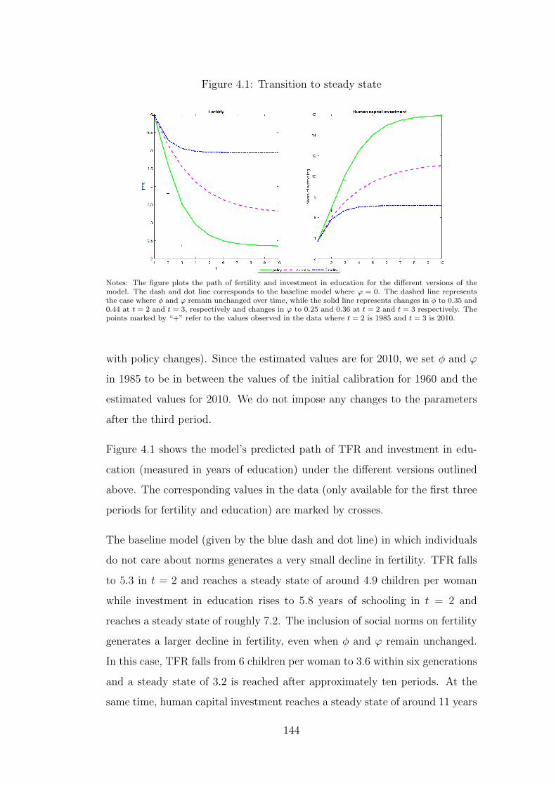
Figure 4.1: Transition to steady state
Notes: The figure plots the path of fertility and investment in education for the different versions of themodel. The dash and dot line corresponds to the baseline model where ϕ = 0. The dashed line representsthe case where φ and ϕ remain unchanged over time, while the solid line represents changes in φ to 0.35 and0.44 at t = 2 and t = 3, respectively and changes in ϕ to 0.25 and 0.36 at t = 2 and t = 3 respectively. Thepoints marked by “+” refer to the values observed in the data where t = 2 is 1985 and t = 3 is 2010.
with policy changes). Since the estimated values are for 2010, we set φ and ϕ
in 1985 to be in between the values of the initial calibration for 1960 and the
estimated values for 2010. We do not impose any changes to the parameters
after the third period.
Figure 4.1 shows the model’s predicted path of TFR and investment in edu-
cation (measured in years of education) under the different versions outlined
above. The corresponding values in the data (only available for the first three
periods for fertility and education) are marked by crosses.
The baseline model (given by the blue dash and dot line) in which individuals
do not care about norms generates a very small decline in fertility. TFR falls
to 5.3 in t = 2 and reaches a steady state of around 4.9 children per woman
while investment in education rises to 5.8 years of schooling in t = 2 and
reaches a steady state of roughly 7.2. The inclusion of social norms on fertility
generates a larger decline in fertility, even when φ and ϕ remain unchanged.
In this case, TFR falls from 6 children per woman to 3.6 within six generations
and a steady state of 3.2 is reached after approximately ten periods. At the
same time, human capital investment reaches a steady state of around 11 years
144

of schooling. The existence of endogenously evolving social norms on fertility
is enough to generate a decline in fertility which is twice as large as the decline
generated by the baseline model.
We now consider the effect of the population control policies (given by the
green solid line), which we interpret as an increase in φ. As can be expected,
the increase in φ (a larger weight placed on the replacement level of fertility)
generates a much larger decline in fertility and increase in education, and a
quicker convergence to the steady state. We allow φ to rise from 0.21 in t = 1
to 0.35 and then 0.44 in the two subsequent periods, which corresponds to a
change in the norm on number of children from around 6 children in the initial
period to around 3.4 by t = 3. Accordingly, the model predicts a decline
in TFR to 3.4 at t = 3 and fertility reaches a steady state of 2.4 after 6
periods. At the same time, years of schooling rises from 4 to around 10 in just
three generations. The increase in ϕ is less important, quantitatively, than the
increase in φ. If we set the starting level of ϕ to 0.36, the resulting transition
path is hardly different from that illustrated in Figure 4.1.
Comparing the results of the model with the data indicates that the inclusion of
social norms with an increase in φ over time improves the predictions of fertility
and years of schooling considerably. The model predicts years of schooling
very well while predicting levels of fertility that are slightly higher than what
is observed in the data. However, the predicted steady state level of fertility is
close to two children per woman. Note that we do not allow φ and ϕ to change
after t = 3. If we allowed φ to increase continuously over time, convergence
to a low, steady-state level of fertility would be even faster. The changes in
φ which would be required to exactly match the data would be an increase to
0.6 in t = 2 and then to 0.9 by t = 3. While we are estimating the change in
φ captured by spending on family planning programmes, it is likely that when
taking into account other factors such as increased access to mass media and
modernisation, the actual increase in φ is larger than that estimated in this
paper.
145

To summarise, this quantitative exercise points to the importance of changing
social norms on family size for the decline in fertility observed in developing
countries over the past few decades. We use data on family planning pro-
gramme funds to capture the change in social norms brought about by these
programmes which were widely adopted in developing countries during this
period. The results suggest that the change in social norms brought about
by these programmes accelerated the fertility decline considerably. While this
confirms the results presented in Chapter 2, it is also consistent with empirical
studies that find evidence of the effectiveness of public persuasion measures
in reducing fertility (La Ferrara, Chong and Duryea 2012 and Bandiera et al.
2014).
4.5 Extensions and robustness checks
In this section we discuss a number of extensions of the model. First, we
extend the model to allow a role for declining infant and child mortality in the
fertility fall. Next, we incorporate imperfect control over fertility, allowing for
a role for improvements in contraceptive technologies. Finally, we consider the
effect of changing the specification of disutility from deviating from the norm,
allowing upward and downward deviations to be treated asymmetrically.
4.5.1 Including mortality
The model presented in the previous section did not take into account the
mortality decline observed in developing countries during this period. In this
section, we extend our model to include uncertainty regarding the number
of children that survive to adulthood. We then investigate the impact of an
increase in survival rates on fertility and human capital investment. We follow
Kalemli-Ozcan (2003) in how we incorporate mortality into the model.14
14In the original Barro-Becker (1989) framework, child mortality is modeled as an explicitcost of childrearing. Doepke (2005) studies three variations of this model: a baseline model
146

Parents choose a number of children, nt, but only Nt of the infants survive
to childhood and all children survive to adulthood. Parents spend on rearing
and educating their surviving children and derive utility from the quantity and
quality of these children.15 In addition, parents care about how the number
of their surviving children compares with the social norm on family size. The
utility function for an adult of generation t can then be written as:
EtUt = Et lnCt + α lnNt + θ ln[wt+1(H +Ht+1)]− ϕ(Nt − Nt)2 (4.12)
where Nt = φn∗ + (1− φ)Nt−1 is the norm on family size.
Expected utility is maximised with respect to
Ct = [1− (τ0 + τ1ht)Nt]wt(H +Ht) (4.13)
and the human capital production function (4.7).
As in Kalemli-Ozcan (2003), Nt is a random variable drawn from a binomial
distribution, with st ∈ [0, 1] the survival probability of each infant. We use a
second order approximation of the expected utility function around the mean
value of Nt, ntst. The approximated expected utility function is given by:
EtUt = Et
ln[(1− (τ0 + τ1ht)ntst)wt(H +Ht)]+
α ln(ntst) + θ ln[wt+1(H +Ht+1)]
−ϕ(ntst − Nt)2 − ntst(1−st)
2[(
(τ0+τ1ht)(τ0+τ1ht)ntst)
)2
+ α(ntst)2
+ 2ϕ]
(4.14)
which incorporates the budget constraint (4.13). The last three terms represent
the disutility arising from uncertainty in the number of infants that survive to
where fertility choice is continuous and there is no uncertainty over the number of surviv-ing children, which is contrasted with an extension involving discrete fertility choice andstochastic mortality and another with sequential fertility choice. He finds that while thetotal fertility rate falls as child mortality declines in each model, the number of survivingchildren increases, and concludes that factors other than declining infant and child mortalitywere responsible for the fertility transition observed in industrialised countries.
15This is a slight deviation from Kalemli-Ozcan (2003) where education is provided beforethe uncertainty is realised.
147

adulthood.
The first order conditions for fertility and human capital investment become:
α
nt(1+
(1− st)2ntst
) =2ϕst(ntst − Nt) + ϕst(1− st)+
(τ0+τ1ht)st1−(τ0+τ1ht)ntst
[1 + 1+(τ0+τ1ht)ntst
2(1−(τ0+τ1ht)ntst)(τ0+τ1ht)(1−st)
(1−(τ0+τ1ht)ntst)
] (4.15)
θzt(H +Ht)
(H +Ht+1)=
τ1ntst(1− (τ0 + τ1ht)ntst)
[1 +
(τ0 + τ1ht)(1− st)(1− (τ0 + τ1ht)ntst)2
](4.16)
The key difference between this setup and that in Section 4.2 is that there is
now an additional term in the marginal cost of both fertility and schooling
which reflects the cost of uncertainty.
Calibration and results
The calibration exercise is carried out in the same way as before - we start
from a model with mortality and no norms to back out all the parameters
except φ and then use the extended model with norms and mortality to get
an initial value for φ. We use the mortality rate for children below 5 years of
age (measured as the number of deaths of children below 5 years of age per
1000 live births) for developing countries in 1960 (from the WDI database) as
a measure of 1 − st. The re-calibration causes τ0, α, θ, and φ to change. τ0,
α and θ change by very little (to 0.05, 0.17 and 0.05, respectively) whereas φ
changes to 0.02, much lower than the φ = 0.21 obtained for the model without
mortality.
To identify the change in φ and ϕ over the past two periods, we carry out the
same estimation exercise as before, again setting φ = φ0 + φ1P but now using
Equation 4.15. We see an increase in φ and ϕ, with a much larger relative
increase in the value of φ than in the model without mortality. Table 4.3
shows the values of the parameters obtained from the estimation.
148

Table 4.3: Estimation of ϕ and φ with mortality
Parameter Valueϕ 0.29
(0.006)φ0 -0.32
(0.118)φ1 0.15
(0.096)φ (= φ0 + φ1P ) 0.21
Observations 50R2 0.37
Notes: The table reports the results from esti-mating Equation 4.15. The estimation is carriedout using data on fertility, child mortality rates,consumption and GDP per capita for 2010, andthe average annual per capita spending on familyplanning over the 1970-2000 period. φ is calculatedas φ = φ0 + φ1P , where P is the sample averageof per capita spending on family planning. Valuesin parentheses are p-values of the regression coeffi-cients from which the values for ϕ, φ0, and φ1 arebacked out and are based on robust standard errors.
We then plot the transition paths of fertility and human capital to their steady
states for three cases: the baseline model with no norms or mortality (given
by the blue dashed line), the model with falling mortality rates and no norms
(given by the pink dotted line), and the extended model of mortality and social
norms (given by the green solid line). We allow st to rise over time from 0.78
in t = 1 to 0.91 and 0.96 in t = 2 and t = 3 as seen in the data. As before,
since the estimation of φ and ϕ was for 2010, values of φ and ϕ for 1985 are set
to be in between the values of the initial calibration for 1960 and the estimates
for 2010, and do not change after the third period.
As figure 4.2 shows, the incorporation of mortality into the baseline model gen-
erates a larger decline in fertility than the baseline model which only includes
human capital accumulation with TFR converging to around 3.9 children per
woman rather than 4.9. However, the two models are not very different in their
predictions of human capital investment. This is because the decline in the
number of surviving children is very similar in these two models (see Figure
4.3). In the baseline model that incorporates the mortality decline, the number
149

Figure 4.2: Incorporating mortality
Notes: The figure plots the path of fertility and investment in education in the three versions of the model.The dashed line represents the baseline model with no mortality or social norms while the dotted linerepresents the baseline model augmented to include mortality where st rises to 0.91 at t=2, and to 0.96 att=3, where it remains in all successive periods. The solid line represents the model with mortality and socialnorms. Here, st rises as described earlier while φ rises to 0.15 and 0.21 in the second and third periods,while ϕ rises to 0.2 and 0.28. The points marked “+” refer to the values observed in the data.
of surviving children drops from 4.7 to just 3.9 (compared to the decline from
5.9 to 4.9 in the baseline model without mortality). By contrast, including
a social norm which falls over time generates a large decline in the number
of surviving children - a drop from 4.6 to 2.6. Given that the investment in
schooling is made for surviving children, a smaller decline in surviving children
leads to a smaller increase in the years of schooling.
Our modelling of mortality, which is based on Kalemli-Ozcan (2003), allows
the mortality decline to generate a decline in fertility through a hoarding effect,
where the risk of child mortality results in a precautionary demand for chil-
dren. The decline in fertility generated by the decline in social norms is slightly
smaller than that in the model described in the previous section because un-
certainty about the number of surviving children leads to higher fertility as an
insurance against infant mortality. However, the presence of social norms that
decline over time still leads to a significant acceleration in the fertility decline,
indicating that the mortality transition cannot rule out the role of the popula-
tion control policies in the fertility fall. Taken as a whole, we would argue that
while the decline in mortality rates did play an important role in triggering
150

Figure 4.3: Number of surviving children
Notes: The figure plots the number of surviving children predicted by the three versions of the model. Thedashed line represents the baseline model with no mortality or social norms while the dotted line representsthe baseline model augmented to include mortality where st rises to 0.91 at t=2, and to 0.96 at t=3, whereit remains in all successive periods. The solid line represents the model with mortality and social norms.
the introduction of population-control policies, its role in precipitating the fast
fall in fertility through individual responses, without the policy intervention,
is less clear.
4.5.2 Incorporating unwanted fertility
So far we have simulated the effect of population control policies on the fertility
decline by focusing on their role in changing the norm on family size. We
now extend the model such that individuals do not perfectly control fertility.
In other words, we allow the lack of contraceptive technologies to cause a
discrepancy between the desired and actual number of children.16 This allows
us to examine the impact of a reduction in unwanted fertility caused by the
introduction of widespread modern contraceptives, which was the second main
component of the population control policies.
We do not explicitly model the choice of contraceptive usage (see, for example,
Cavalcanti, Kocharkov and Santos (2017)) but consider individuals’ ability to
16The key difference between this and the mortality extension is that now individuals facethe risk of overshooting their desired number of children whereas in the case of uncertaintyabout mortality, individuals faced the risk of ending up with less children than they wanted.
151

control fertility to be exogenously determined. So while the production side of
the model is the same as before, we now assume that parents’ inability to per-
fectly control their fertility leads to a distinction between the desired or chosen
number of children, ndt , and the actual number of children, nat . Specifically,
nat = ndt + εt,
where εt is a stochastic error term causing the desired number of children, ndt ,
to differ from the actual number of children, nat .
Individuals now have to maximize expected utility which, for an adult of gen-
eration t is given by:
EtUt = Et[lnCt + α lnnat + θ ln[wt+1(H +Ht+1)]− ϕ(nat − nt)2], (4.17)
where Et denotes expectations as of time t.
Individuals maximize expected utility with respect to the human capital pro-
duction function (same as before) and the budget constraint, which is now
changed slightly to
Ct = [1− (τ0 + τ1ht)nat ]wt(H +Ht) (4.18)
The formulation of the expected utility function requires some distributional
assumptions about unwanted fertility, εt. The data on wanted fertility rates
in developing countries (obtained from Demographic and Health Surveys) in-
dicates that εt is usually positive and has a positively skewed distribution. As
such, we assume that εt follows a Poisson distribution with mean λ. Thus,
a reduction in λ translates to a reduction in uncertainty as well as average
unwanted fertility. We then carry out a second order approximation of the ex-
pected utility around the mean of unwanted fertility. Substituting in the bud-
get constraint and human capital production function, the household problem
152

can be rewritten as:
{ndt , ht} = arg max
ln[(1− (τ0 + τ1ht)(ndt + λ))wt(H +Ht)]
+θ ln[Wt+1(H + zt(H +Ht)ht)]
+α ln[ndt + λ]− ϕ(ndt + λ− nt)2
−λ2[ (τ0+τ1ht)2
(1−(τ0+τ1ht)(ndt +λ))2
+ 2ϕ+ α(nd
t +λ)2]
(4.19)
subject to: (ndt , ht) ≥ 0.
The first order conditions for ndt and ht are given by
α
ndt + λ=
(τ0+τ1ht)
(1−(τ0+τ1ht)(ndt +λ))
+ 2ϕ(ndt + λ− nt)+
λ[ (τ0+τ1ht)3
(1−(τ0+τ1ht)(ndt +λ))3
− α(nd
t +λ)3]
(4.20)
θzt(H +Ht)
(H +Ht+1)=
τ1(ndt + λ)
(1− (τ0 + τ1ht)(ndt + λ))+ λ[
τ1(τ0 + τ1ht)
(1− (τ0 + τ1ht)(ndt + λ))3]
(4.21)
where the last term on the right hand side in Equation 4.21 reflects the cost of
uncertainty. Since parents derive utility from all children (unwanted or not),
the second line on the right hand side of Equation 4.20 reflects the cost of
uncertainty adjusted for the gain in utility caused by having an extra child.
Calibration and results
The calibration strategy follows the same procedure as the main model, leav-
ing parameters α, θ, τ0, τ1, gH , ρ, n∗, and the initial conditions unchanged.
However, φ needs to be recalibrated using Equation 4.20 for given values of ϕ
and λ. λ is chosen using data on wanted fertility rates obtained from Demo-
graphic and Health Surveys which start in the late 1980s. Unwanted fertility
(calculated as the difference between TFR and wanted fertility rate) is around
1 birth, on average, in the 1980s. Since this is well after the introduction of the
oral contraceptive pill and the implementation of many family planning pro-
153
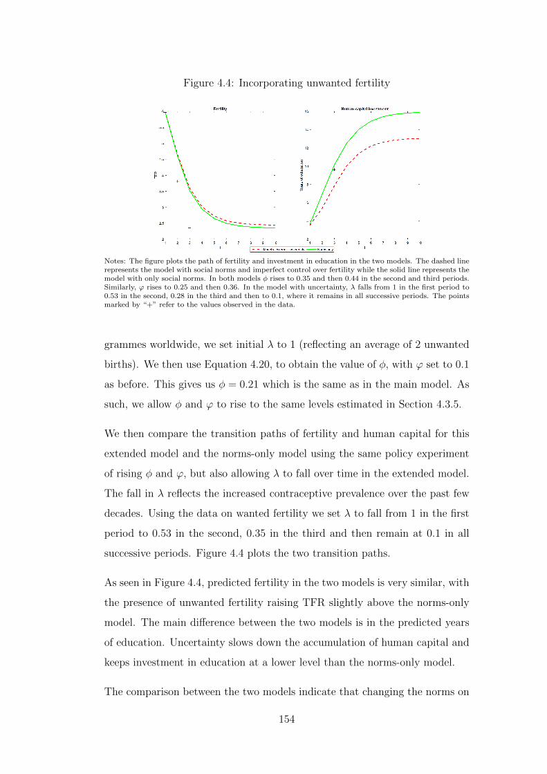
Figure 4.4: Incorporating unwanted fertility
Notes: The figure plots the path of fertility and investment in education in the two models. The dashed linerepresents the model with social norms and imperfect control over fertility while the solid line represents themodel with only social norms. In both models φ rises to 0.35 and then 0.44 in the second and third periods.Similarly, ϕ rises to 0.25 and then 0.36. In the model with uncertainty, λ falls from 1 in the first period to0.53 in the second, 0.28 in the third and then to 0.1, where it remains in all successive periods. The pointsmarked by “+” refer to the values observed in the data.
grammes worldwide, we set initial λ to 1 (reflecting an average of 2 unwanted
births). We then use Equation 4.20, to obtain the value of φ, with ϕ set to 0.1
as before. This gives us φ = 0.21 which is the same as in the main model. As
such, we allow φ and ϕ to rise to the same levels estimated in Section 4.3.5.
We then compare the transition paths of fertility and human capital for this
extended model and the norms-only model using the same policy experiment
of rising φ and ϕ, but also allowing λ to fall over time in the extended model.
The fall in λ reflects the increased contraceptive prevalence over the past few
decades. Using the data on wanted fertility we set λ to fall from 1 in the first
period to 0.53 in the second, 0.35 in the third and then remain at 0.1 in all
successive periods. Figure 4.4 plots the two transition paths.
As seen in Figure 4.4, predicted fertility in the two models is very similar, with
the presence of unwanted fertility raising TFR slightly above the norms-only
model. The main difference between the two models is in the predicted years
of education. Uncertainty slows down the accumulation of human capital and
keeps investment in education at a lower level than the norms-only model.
The comparison between the two models indicate that changing the norms on
154

fertility has a much larger effect on fertility decisions than merely increasing
access to contraception. This is consistent with the fact that many of the family
planning programmes supplemented their supply-side strategies of increasing
access to contraception with large scale mass media campaigns to promote
smaller family sizes. This point was made by demographers Enke (1960) and
Davis (1967) at early stages of the global population control movement, and
later by Becker (1992), who argued that family planning programmes focused
on increasing contraceptive usage are effective only when the value of having
children is lowered.
4.5.3 Functional form of disutility from deviation from
the norm
We now consider the robustness of our results to an alternative specification
for the disutility from deviating from the norm. In particular, we now use a
functional form that treats upward and downward deviations from the norm
asymmetrically with deviations below the norm being penalised more heav-
ily than deviations above. This would be consistent with societal norms in
developing countries where not having children is considered taboo. For this
purpose, we set:
g(nt, n) = [ln(nt/nt)]2
The first order condition for fertility changes to the following:
α
nt=
(τ0 + τ1ht)
(1− (τ0 + τ1ht)nt)+ 2ϕ
1
ntln(nt/nt) (4.22)
while the first order condition for human capital investment remains unchanged.
Under the same parameter values and initial conditions as in the previous
section, we plot the transition paths of fertility and investment in human
capital to their steady state values. We consider two experiments: one in which
φ and ϕ increase and the other in which both parameters remain unchanged
155
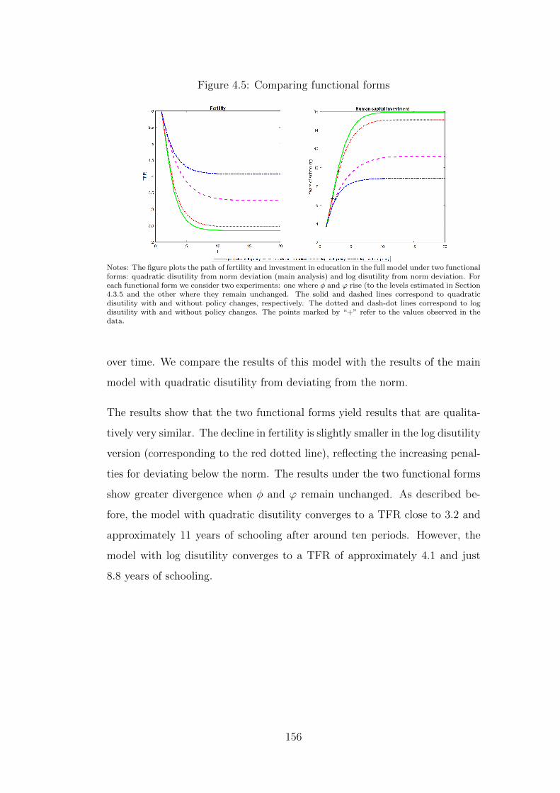
Figure 4.5: Comparing functional forms
Notes: The figure plots the path of fertility and investment in education in the full model under two functionalforms: quadratic disutility from norm deviation (main analysis) and log disutility from norm deviation. Foreach functional form we consider two experiments: one where φ and ϕ rise (to the levels estimated in Section4.3.5 and the other where they remain unchanged. The solid and dashed lines correspond to quadraticdisutility with and without policy changes, respectively. The dotted and dash-dot lines correspond to logdisutility with and without policy changes. The points marked by “+” refer to the values observed in thedata.
over time. We compare the results of this model with the results of the main
model with quadratic disutility from deviating from the norm.
The results show that the two functional forms yield results that are qualita-
tively very similar. The decline in fertility is slightly smaller in the log disutility
version (corresponding to the red dotted line), reflecting the increasing penal-
ties for deviating below the norm. The results under the two functional forms
show greater divergence when φ and ϕ remain unchanged. As described be-
fore, the model with quadratic disutility converges to a TFR close to 3.2 and
approximately 11 years of schooling after around ten periods. However, the
model with log disutility converges to a TFR of approximately 4.1 and just
8.8 years of schooling.
156

4.6 Conclusion
In this paper, we present a tractable model that allows us to quantitatively
assess the role of different mechanisms driving the large declines in fertility
experienced by developing countries over the past few decades. In particu-
lar, we examine the role of population-control policies aimed at affecting so-
cial norms and fostering contraceptive technologies. The model builds on the
Barro-Becker framework of endogenous fertility choice, incorporating human
capital accumulation and social norms over the number of children. Using data
on several socio-economic variables as well as information on funding for family
planning programmes to parametrise the model, we simulate the implementa-
tion of population-control policies. We also consider several extensions such
as adding a role for the mortality decline and improvements in contraceptive
technologies. The model suggests that, while a decline in fertility would have
gradually taken place as economies move to higher levels of human capital and
lower levels of infant and child mortality, policies aimed at altering the norms
on family size significantly accelerate and strengthen the decline.
157
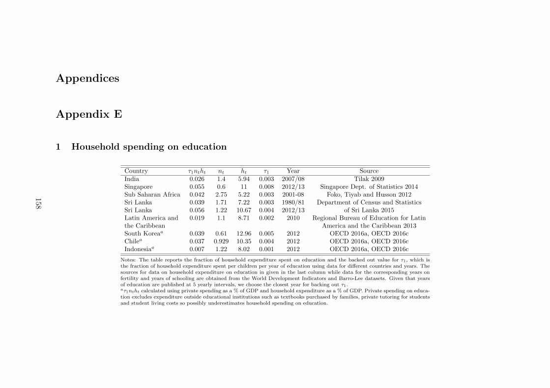
Appendices
Appendix E
1 Household spending on education
Country τ1ntht nt ht τ1 Year SourceIndia 0.026 1.4 5.94 0.003 2007/08 Tilak 2009Singapore 0.055 0.6 11 0.008 2012/13 Singapore Dept. of Statistics 2014Sub Saharan Africa 0.042 2.75 5.22 0.003 2001-08 Foko, Tiyab and Husson 2012Sri Lanka 0.039 1.71 7.22 0.003 1980/81 Department of Census and StatisticsSri Lanka 0.056 1.22 10.67 0.004 2012/13 of Sri Lanka 2015Latin America and 0.019 1.1 8.71 0.002 2010 Regional Bureau of Education for Latinthe Caribbean America and the Caribbean 2013South Koreaa 0.039 0.61 12.96 0.005 2012 OECD 2016a, OECD 2016cChilea 0.037 0.929 10.35 0.004 2012 OECD 2016a, OECD 2016cIndonesiaa 0.007 1.22 8.02 0.001 2012 OECD 2016a, OECD 2016c
Notes: The table reports the fraction of household expenditure spent on education and the backed out value for τ1, which isthe fraction of household expenditure spent per children per year of education using data for different countries and years. Thesources for data on household expenditure on education in given in the last column while data for the corresponding years onfertility and years of schooling are obtained from the World Development Indicators and Barro-Lee datasets. Given that yearsof education are published at 5 yearly intervals, we choose the closest year for backing out τ1.aτ1ntht calculated using private spending as a % of GDP and household expenditure as a % of GDP. Private spending on educa-tion excludes expenditure outside educational institutions such as textbooks purchased by families, private tutoring for studentsand student living costs so possibly underestimates household spending on education.
158

Bibliography
Akerlof, G. (1976). The Economics of Caste and of the Rat Race and Other
Woeful Tales. The Quarterly Journal of Economics, 90(4):599–617.
Akerlof, G. (1997). Social Distance and Social Decisions. Econometrica,
65(5):1005–1028.
Akin, A. (2007). Emergence of the Family Planning Program in Turkey. In
Robinson, W. C. and Ross, J. A., editors, The Global Family Planning Rev-
olution: Three Decades of Population Policies and Programs, pages 85–102.
World Bank.
Anderson, T. and Kohler, H.-P. (2013). Education Fever and the East Asian
Fertility Puzzle. Asian Population Studies, 9(2):196–215.
Angrist, J. and Pischke, J.-S. (2009). Mostly Harmless Econometrics: An
Empiricist’s Companion. Princeton University Press, First edition.
Attane, I. (2002). China’s Family Planning Policy: An Overview of Its Past
and Future. Studies in Family Planning, 33(1):103–113.
Bailey, M. J. (2013). Fifty Years of Family Planning: New evidence on the
long-run effects of increasing access to contraception. Brookings Papers on
Economic Activity, 46(1):341–409.
Bandiera, O., Buehren, N., Burgess, R., Goldstein, M., Gulesci, S., Rasul,
I., and Sulaiman, M. (2014). Women’s Empowerment In Action: Evi-
dence From A Randomised Control Trial In Africa. Technical Report 50,
STICERD, LSE, London.
159

Banerjee, A. V., Cole, S., Duflo, E., and Linden, L. (2007). Remedying Educa-
tion: Evidence from Two Randomized Experiments in India. The Quarterly
Journal of Economics, 122(3):1235–1264.
Barro, R. J. and Becker, G. S. (1989). Fertility Choice in a Model of Economic
Growth. Econometrica, 57(2):481–501.
Barro, R. J. and Lee, J. W. (2013). A new data set of educational attainment
in the world, 1950-2010. Journal of Development Economics, 104:184 – 198.
Barro, R. J. and Lee, J. W. (2015). Education Matters: Global Schooling Gains
from the 19th to the 21st Century. Oxford University Press.
Becker, G. S. (1960). An Economic Analysis of Fertility. In NBER, editor, De-
mographic and Economic Change in Developed Countries, chapter 7, pages
209–40. Columbia University Press.
Becker, G. S. (1992). Fertility and the Economy. Journal of Population Eco-
nomics, 5(3):185–201.
Becker, G. S. and Barro, R. J. (1988). A Reformulation of the Economic
Theory of Fertility. The Quarterly Journal of Economics, 103(1):1–25.
Becker, G. S., Murphy, K. M., and Tamura, R. (1990). Human Capital, Fer-
tility, and Economic Growth. Journal of Political Economy, 98(5):S12–S37.
Begum, H. (1993). Family Planning and Social Position of Women. Bioethics,
7(2-3):218–223.
Bertrand, J. T., Ward, V. M., and Santiso-Galvez, R., editors (2015). Family
Planning in Latin America and the Caribbean: The Achievements of 50
Years. MEASURE Evaluation.
Bhattacharya, J. and Chakraborty, S. (2012). Fertility Choice under Child
Mortality and Social Norms. Economics Letters, 115(3):338 – 341.
Bodoh-Creed, A. L. and Hickman, B. R. (2016). College Assignment as a Large
Contest. Manuscript submitted for publication.
160

Boldrin, M. and Jones, L. (2002). Mortality, Fertility, and Saving in a Malthu-
sian Economy. Review of Economic Dynamics, 5(4):775–814.
Bongaarts, J. (2011). Can Family Planning Programs Reduce High Desired
Family Size in Sub-Saharan Africa? International Perspectives on Sexual
and Reproductive Health, 37(4):209–16.
Bound, J., Hershbein, B., and Long, B. T. (2009). Playing the Admissions
Game: Student Reactions to Increasing College Competition. Journal of
Economic Perspectives, 23(4):119–146.
Bray, M. and Lykins, C. (2012). Shadow Education Private Supplementary
Tutoring and Its Implications for Policy Makers in Asia. ADB, Philippines.
Brown, G. F. (2007a). Morocco: First steps in family planning. In Robinson,
W. C. and Ross, J. A., editors, The Global Family Planning Revolution:
Three Decades of Population Policies and Programs, pages 71–82. World
Bank.
Brown, G. F. (2007b). Tunisia: The Debut of Family Planning. In Robinson,
W. C. and Ross, J. A., editors, The Global Family Planning Revolution:
Three Decades of Population Policies and Programs, chapter 4, pages 59–
70. World Bank.
Caldwell, J. C. (1976). Toward A Restatement of Demographic Transition
Theory. Population and Development Review, 2(3/4):321–366.
Caldwell, J. C. and Sai, F. T. (2007). Family Planning in Ghana. In Robinson,
W. C. and Ross, J. A., editors, The Global Family Planning Revolution:
Three Decades of Population Policies and Programs, pages 379–91. World
Bank.
Card, D. and Krueger, A. (1992). Does School Quality Matter? Returns to
Education and the Characteristics of Public Schools in the United States.
Journal of Political Economy, 100(1):1–40.
161

Cavalcanti, T., Kocharkov, G., and Santos, C. (2017). Family Plan-
ning and Development: Aggregate Effects of Contraceptive Use.
http://pareto.uab.es/research/sempdf/macro/2017/Contraception.pdf.
[Accessed on 30 June 2017].
Cavenaghi, S., editor (2009). Demographic transformations and inequalities
in Latin America. Series Investigaciones No. 8. Latin American Population
Association, Rio de Janeiro.
Cespedes, Luis Felipeand Velasco, A. (2012). Macroeconomic Performance
During Commodity Price Booms and Busts. IMF Economic Review,
60(4):570–599.
Choi, H. and Choi, A. (2015). When One Door Closes: The Impact of the
Hagwon Curfew on the Consumption of Private Tutoring in the Republic
of Korea. Working paper 2015/26 1/34, Regional Institute of Applied Eco-
nomics, Universitat de Barcelona, Barcelona.
Choi, H. J. and Park, J.-H. (2013). Historical Analysis of the Policy on the
College Entrance System in South Korea. International Education Studies,
6(11):106–121.
Choi, J. and Cho, R. M. (2016). Evaluating the Effects of Governmental
Regulations on South Korean Private Cram Schools. Asia Pacific Journal
of Education, 36(4):599–621.
Choukhmane, T., Coeurdacier, N., and Jin, K. (2014). The One-Child Policy
and Household Savings. Sciences Po publications, Sciences Po, Paris.
Church, C. A. and Geller, J. (1989). Lights! Camera! Action! Promoting
family planning with TV, video and film. Population Reports, 17(5):2–31.
Clay, D. and Zuiches, J. (1980). Reference Groups and Family Size Norms.
Population and Environment, 3(3-4):262–279.
162

Coale, A. J. (1969). The Decline Of Fertility In Europe From The French
Revolution to World War II. In Behrman, S. and Corsa, L., editors, Fertility
and Family Planning: A World View, chapter 1, pages 3–24. The University
of Michigan Press.
Coeurdacier, N., Guibaud, S., and Jin, K. (2014). Fertility Policies and Social
Security Reforms in China. IMF Economic Review, 62(3):371–408.
Dang, H.-A. (2007). The Determinants and Impact of Private Tutoring Classes
in Vietnam. Economics of Education Review, 26(6):683–698.
Davis, K. (1967). Population Policy: Will Current Programs Succeed? Science,
158(3802):730–739.
Demographic and Health Survey Program (2015). The DHS Program STAT-
compiler. www.statcompiler.com. [Accessed on June 18, 2015].
Department of Census and Statistics (2015). Household Income and Expendi-
ture Survey 2012/13: Final report. Technical report, Department of Census
and Statistics of Sri Lanka, Colombo, Sri Lanka.
Department of Statistics (2014). Report on the Household Expenditure Sur-
vey 2012/13. Technical report, Ministry of Trade and Industry, Singapore,
Singapore.
Doepke, M. (2004). Accounting for Fertility Decline during the Transition to
Growth. Journal of Economic Growth, 9(3):pp. 347–383.
Doepke, M. (2005). Child Mortality and Fertility Decline: Does the Barro-
Becker model fit the facts? Journal of Population Economics, 18(2):337–
366.
Dong, Y. and Lewbel, A. (2015). A Simple Estimator for Binary Choice Models
with Endogenous Regressors. Econometric Reviews, 34(1-2):82–105.
Draper, W. H. (1959). Composite Report of the President’s Committee to
study the U.S. Military Assistance Program. Technical report.
163

Duflo, E. (2001). Schooling and Labor Market Consequences of School Con-
struction in Indonesia: Evidence from an Unusual Policy Experiment. Amer-
ican Economic Review, 91(4):795–813.
Ehrlich, I. and Kim, J. (2005). Endogenous fertility, mortality and economic
growth: Can a Malthusian framework account for the conflicting historical
trends in population? Journal of Asian Economics, 16(5):789–806.
Enke, S. (1960). The Economics of Government Payments to Limit Population.
Economic Development and Cultural Change, 8(4):339–348.
Fan, S. (2007). Hong Kong: Evolution Of The Family Planning Program.
In Robinson, W. C. and Ross, J. A., editors, The Global Family Planning
Revolution: Three Decades of Population Policies and Programs, chapter 12,
pages 193–200. World Bank.
Foko, B., Tiyab, B. K., and Husson, G. (2012). Household education spend-
ing: An Analytical and Comparative Perspective for 15 African Countries.
Technical report, UNESCO, Dakar, Senegal.
Freedman, R. and Berelson, B. (1976). The Record of Family Planning Pro-
grams. Studies in Family Planning, 7(1):1–40.
Fu, Q. (2003). A Theory of Affirmative Action in College Admissions: An
All-Pay Auction Approach. Unpublished.
Galor, O. and Moav, O. (2002). Natural Selection and the Origin of Economic
Growth. The Quarterly Journal of Economics, 117(4):1133–1191.
Galor, O. and Weil, D. N. (2000). Population, Technology, And Growth: From
Malthusian Stagnation To The Demographic Transition And Beyond. The
American Economic Review, 90(4):806–828.
Gilluly, R. H. and Moore, S. (1986). Radio - spreading the word on family
planning. Population Reports, 14(4):854–86.
164
Goldin, C. and Katz, L. F. (2002). The Power of the Pill: Oral contraceptives
and women’s career and marriage decisions. Journal of Political Economy,
110(4):730–770.
Grubb, W. N., Sweet, R., Gallagher, M., and Tuomi, O. (2009). Korea. OECD
reviews of tertiary education, OECD.
Hafalir, I. E., Hakimov, R., Kubler, D., and Kurino, M. (2016). College Ad-
missions with Entrance Exams: Centralized versus Decentralized. SFB 649
Discussion Papers, Humboldt University, Berlin.
Harkavy, O. and Roy, K. (2007). Emergence Of The Indian National Fam-
ily Planning Program. In Robinson, W. C. and Ross, J. A., editors, The
Global Family Planning Revolution: Three Decades of Population Policies
and Programs, chapter 18, pages 301–324. World Bank.
Heisel, D. F. (2007). Family Planning in Kenya in the 1960s and 1970s. In
Robinson, W. C. and Ross, J. A., editors, The Global Family Planning Revo-
lution: Three Decades of Population Policies and Programs, pages 393–417.
World Bank.
Herrin, A. N. (2007). Development of the Philippines’ Family Planning Pro-
gram: The Early Years, 1967-80. In Robinson, W. C. and Ross, J. A.,
editors, The Global Family Planning Revolution: Three Decades of Popula-
tion Policies and Programs, pages 277–97. World Bank.
Hogan, H., Kennedy, B. L., Obetsebi-Lamptey, J., and Sawaya, S. (1985).
Mauritius: Population and Family Planning Assessment. Technical report,
USAID.
Hopkins, E. and Kornienko, T. (2010). Which Inequality? The Inequality of
Endowments versus the Inequality of Rewards. American Economic Journal:
Microeconomics, 2(3):106–37.
Hull, T. H. (2007). Formative Years Of Family Planning In Indonesia. In
Robinson, W. C. and Ross, J. A., editors, The Global Family Planning Rev-
165

olution: Three Decades of Population Policies and Programs, chapter 15,
pages 235–256. World Bank.
Jacob, B. A. and Lefgren, L. (2004). Remedial Education and Student Achieve-
ment: A Regression-Discontinuity Analysis. The Review of Economics and
Statistics, 86(1):226–244.
Jones, S. R. G. (1984). The Economics of Conformism. Basil Blackwell,
Oxford.
Kalemli-Ozcan, S. (2002). Does the Mortality Decline Promote Economic
Growth? Journal of Economic Growth, 7(4):411–439.
Kalemli-Ozcan, S. (2003). A Stochastic Model of Mortality, Fertility, and
Human Capital Investment. Journal of Development Economics, 70(1):103–
118.
Kang, C. (2007). Does Money Matter? The Effect of Private Educational
Expenditures on Academic Performance. Departmental Working Papers
WP0704, National University of Singapore, Department of Economics.
KESS (2017a). Number of Higher Education Institutes, Schools.
http://kess.kedi.re.kr/eng. [Accesssed on 31 March 2017].
KESS (2017b). Number of Students in Higher Education Institutes, Schools.
http://kess.kedi.re.kr. [Accesssed on 31 March 2017].
Khanna, S. (2009). Population Growth and “Missing” girls. In Fetal/Fatal
Knowledge: New Reproductive Technologies and Family-Building Strategies
in India (CSCSI), chapter 4, pages 57–74. Cengage Learning.
Kim, T. I. and Ross, J. A. (2007). The Korean Breakthrough. In Robinson,
W. C. and Ross, J. A., editors, The Global Family Planning Revolution:
Three Decades of Population Policies and Programs, chapter 11, pages 177–
192. World Bank.
166

King, T. (2007). Family Planning And The World Bank In Jamaica. In Robin-
son, W. C. and Ross, J. A., editors, The Global Family Planning Revolution:
Three Decades of Population Policies and Programs, chapter 10, pages 155–
174. World Bank.
Kolk, M. (2014). Multigenerational Transmission of Family Size in Contem-
porary Sweden. Population studies, 68(1):111–129.
KOSIS (2017a). Average Monthly Income and Expenditure.
http://kosis.kr/eng. [Accesssed on 31 March 2017].
KOSIS (2017b). Number of Internal Migrants by Origin and Destination, Sex,
and Five-year Age Groups for Province. http://kosis.kr/eng. [Accesssed on
01 May 2017].
KOSIS (2017c). Private Education Participation Rate by Education Level.
http://kosis.kr/eng. [Accesssed on 31 March 2017].
La Ferrara, E., Chong, A., and Duryea, S. (2012). Soap Operas And Fertility:
Evidence From Brazil. American Economic Journal: Applied Economics,
4(4):1–31.
Landers, R. M., Rebitzer, J., and Taylor, L. J. (1996). Rat Race Redux: Ad-
verse Selection in the Determination of Work Hours in Law Firms. American
Economic Review, 86(3):329–48.
Lapham, R. and Mauldin, W. (1984). Family Planning Program Effort and
Birthrate Decline in Developing Countries. International Family Planning
Perspectives, 10(4):109–118.
Lavy, V. and Schlosser, A. (2005). Targeted Remedial Education for Under-
performing Teenagers: Costs and Benefits. Journal of Labor Economics,
23(4):839–874.
Lee, C. J., Lee, H., and Jang, H.-M. (2010). The History of Policy Responses
to Shadow Education in South Korea: Implications for the next cycle of
policy responses. Asia Pacific Education Review, 11(1):97–108.
167
Liang, Q. and Lee, C.-F. (2006). Fertility and Population Policy: an Overview.
In Poston, D. L., Lee, C.-F., Chang, C.-F., McKibben, S. L., and Walther,
C. S., editors, Fertility, Family Planning and Population Policy in China,
pages 7–18. Routledge.
Machin, S. and McNally, S. (2007). Tertiary Education Systems and Labour
Markets. Technical report, OECD.
Manuelli, R. E. and Seshadri, A. (2009). Explaining International Fertility
Differences. The Quarterly Journal of Economics, 124(2):771–807.
Measham, A. R. and Lopez-Escobar, G. (2007). Against the Odds: Colombia’s
Role in the Family Planning Revolution. In Robinson, W. C. and Ross,
J. A., editors, The Global Family Planning Revolution: Three Decades of
Population Policies and Programs, pages 121–35. World Bank.
Moav, O. (2005). Cheap Children and the Persistence of Poverty. The Eco-
nomic Journal, 115:88–110.
Moore, R. (2007). Family Planning In Iran, 1960-79. In Robinson, W. C. and
Ross, J. A., editors, The Global Family Planning Revolution: Three Decades
of Population Policies and Programs, chapter 3. World Bank.
Munshi, K. and Myaux, J. (2006). Social Norms and the Fertility Transition.
Journal of Development Economics, 80(1):1–38.
Murphy, M. (1999). Is the Relationship Between Fertility of Parents and Chil-
dren Really Weak? Social biology, 46(1-2):122–145.
National Research Council Working Group on Factors Affecting Contraceptive
Use (1993). Factors Affecting Contraceptive Use in Sub-Saharan Africa.
Technical report, National Research Council, Washington, D.C.
National Security Council (1974). National Security Study Memorandum 200:
Implications of Worldwide Population Growth for U.S. Security and Over-
seas Interests (The Kissinger Report). Technical report, National Security
Council, Washington, D.C.
168

Nortman, D. L. (1982). Population and Family Planning Programs: A Com-
pendium of Data through 1981. The Population Council, New York, 11th
edition.
Nortman, D. L. and Hofstatter, E. (1978). Population and Family Planning
Programs. The Population Council, New York, 9th edition.
OECD (2010). PISA 2009 Results: What Makes a School Successful? Re-
sources, Policies and Practices (Volume IV). Technical report, OECD.
OECD (2016a). Household Expenditure (indicator).
https://data.oecd.org/hha/household-spending.htm. [Accessed on 30
January 2017].
OECD (2016b). PISA 2015 Results (Volume II): Policies and Practices for
Successful Schools. Technical report, OECD.
OECD (2016c). Private Spending on Education (indicator).
https://data.oecd.org/eduresource/private-spending-on-education.htm.
[Accessed on 30 January 2017].
Ono, H. (2007). Does Examination Hell Pay Off? A cost-benefit analysis of
“ronin” and college education in Japan. Economics of Education Review,
26(3):271–284.
Pacini, D. and Windmeijer, F. (2016). Robust inference for the Two-Sample
2SLS estimator. Economics Letters, 146(C):50–54.
Palivos, T. (2001). Social Norms, Fertility and Economic Development. Jour-
nal of Economic Dynamics and Control, 25(12):1919–1934.
Piotrow, P. T. (1973). World Population Crisis: The United States response.
Praeger Publishers.
Piotrow, P. T. and Kincaid, D. L. (2001). Strategic Communications for Inter-
national Health Programs. In Rice, R. E. and Atkin, C. K., editors, Public
169

Communication Campaigns, chapter 14, pages 249–68. Sage Publications,
3rd edition.
Pischke, J.-S. and von Wachter, T. (2008). Zero Returns to Compulsory School-
ing in Germany: Evidence and Interpretation. The Review of Economics and
Statistics, 90(3):592–598.
Population Media Centre (2016). TV Globo analysis: Brazil.
http://populationmedia.org/projects/tv-globo-analysis/. [Accesssed on
February 12, 2016].
Ramey, G. and Ramey, V. A. (2010). The Rug Rat Race. Brookings Papers
on Economic Activity, 41(1 (Spring):129–199.
Regional Bureau of Education for Latin America and the Caribbean (2013).
The State of Education in Latin America and the Caribbean: Towards a
Quality Education for All. Technical report, UNESCO, Santiago.
Rinehart, W., Blackburn, R., and Moore, S. (1987). Employment-based family
planning programs. Population Reports, 15(2):921–51.
Robinson, W. C. (2007). Family planning programs and policies in Bangladesh
and Pakistan. In Robinson, W. C. and Ross, J. A., editors, The Global
Family Planning Revolution: Three Decades of Population Policies and Pro-
grams, pages 325–39. World Bank.
Robinson, W. C. and El-Zanaty, F. H. (2007). The Evolution Of Population
Policies And Programs In The Arab Republic Of Egypt. In Robinson, W. C.
and Ross, J. A., editors, The Global Family Planning Revolution: Three
Decades of Population Policies and Programs, chapter 2. World Bank.
Robinson, W. C. and Ross, J. A., editors (2007). The Global Family Planning
Revolution: Three decades of population policies and programs. World Bank.
Rockefeller, J. D. (1934). RE: Birth Con-
trol Rockefeller, John D. 3rd 1934-03-17.
170
http://rockefeller100.org/files/original/70d2ba6c2a6bddabd46a3cdff4b105c7.pdf.
[Accesssed on March 31, 2017].
Rockefeller, J. D. (1978). Population Growth: The Role of the Developed
World. Population and Development Review, 4(3):509–516.
Rosenfield, A. G. and Min, C. J. (2007). The emergence of Thailand’s National
Family Planning Program. In Robinson, W. C. and Ross, J. A., editors, The
Global Family Planning Revolution: Three Decades of Population Policies
and Programs, pages 221–33. World Bank.
Ross, J. and Stover, J. (2001). The Family Planning Program Effort Index:
1999 cycle. International Family Planning Perspectives, 27(3):119–129.
Ross, J. A., Maudlin, W. P., and Miller, V. C. (1993). Family Planning
and Population: A compendium of international statistics. The Population
Council, New York.
Rutstein, S. O. and Rojas, G. (2006). Guide to DHS Statistics. Technical
report, USAID.
Ryu, D. and Kang, C. (2013). Do Private Tutoring Expenditures Raise Aca-
demic Performance? Evidence from Middle School Students in South Korea.
Asian Economic Journal, 27(1):59–83.
Sanhueza, H. (2007). Family Planning in Chile: A tale of the unexpected.
In Robinson, W. C. and Ross, J. A., editors, The Global Family Planning
Revolution: Three Decades of Population Policies and Programs, pages 105–
20. World Bank.
Santiso-Galvez, R. and Bertrand, J. T. (2007). Guatemala: The pioneering
days of the family planning movement. In Robinson, W. C. and Ross, J. A.,
editors, The Global Family Planning Revolution: Three Decades of Popula-
tion Policies and Programs, pages 137–54. World Bank.
171

Schuler, S. R., Hashemi, S. M., and Jenkins, A. H. (1995). Bangladesh’s
Family Planning Success Story: A Gender Perspective. International Family
Planning Perspectives, 21(4):132–166.
Shaffer, H. (1968). Birth control in Latin America. Technical report, Congres-
sional Quarterly Press, Washington, D.C.
Sherris, J. D. and Quillin, W. (1982). Population Education in the Schools.
Population Reports, 10(2):201–43.
Sicherman, N. (1991). “Overeducation” in the Labor Market. Journal of Labor
Economics, 9(2):101–22.
Sinding, S. W. (2007). Overview and Perspectives. In Robinson, W. C. and
Ross, J. A., editors, The Global Family Planning Revolution: Three Decades
of Population Policies and Programs, chapter 1, pages 1–12. World Bank.
Spence, M. (1973). Job Market Signaling. The Quarterly Journal of Eco-
nomics, 87(3):355.
Sun, T.-H. (2001). The Impacts of a Family Planning Program on Contracep-
tive/Fertility Behaviour in Taiwan. Journal of Population Studies, 23:49–92.
Suryadarma, D., Suryahadi, A., Sumarto, S., and Rogers, F. (2006). Improving
Student Performance in Public Primary Schools in Developing Countries:
Evidence from Indonesia. Education Economics, 14(4):401–429.
Teng, Y. M. (2007). Singapore: Population Policies and Program. In Robin-
son, W. C. and Ross, J. A., editors, The Global Family Planning Revolu-
tion: Three Decades of Population Policies and Programs, chapter 13. World
Bank.
Tey, N. P. (2007). The Family Planning Program In Peninsular Malaysia.
In Robinson, W. C. and Ross, J. A., editors, The Global Family Planning
Revolution: Three Decades of Population Policies and Programs, chapter 16.
World Bank.
172

The World Bank (2015). World Development Indicators.
http://data.worldbank.org/data-catalog/world-development-indicators.
[Accessed on July 20, 2015].
Therborn, G. (2004). Between Sex and Power: Family in the World 1900-2000.
Routledge.
Thornton, A. (1980). The Influence of First Generation Fertility and Eco-
nomic Status on Second Generation Fertility. Population and Environment,
3(1):51–72.
Tien, H. (1980). Wan, Xi, Shao: How China Meets Its Population Problem.
International Family Planning Perspectives, 6(2):65–73.
Tilak, J. B. G. (2009). Household Expenditure on Education and Implica-
tions for Redefining the Poverty Line in India. Technical report, Planning
Commission of India. (Draft).
Tuladhar, J. M. (2007). Emergence and Development of Nepal’s Family Plan-
ning Program. In Robinson, W. C. and Ross, J. A., editors, The Global
Family Planning Revolution: Three Decades of Population Policies and Pro-
grams, pages 363–76. World Bank.
United Nations Population Division (2013). World Population Policies
Database: 2013 Revision. http://esa.un.org/poppolicy/wpp-datasets.aspx.
[Accessed on July 20, 2015].
United Nations Population Division (2015). World Population Prospects: The
2015 Revision, Key Findings and Advance Tables. Technical report, UN.
Wang, C. (2012). History of the Chinese Family Planning program: 1970-2010.
Contraception, 85(6):563 – 569.
Wright, N. H. (2007). Early Family Planning Efforts In Sri Lanka. In Robin-
son, W. C. and Ross, J. A., editors, The Global Family Planning Revolu-
tion: Three Decades of Population Policies and Programs, chapter 20. World
Bank.
173

Young, A. (1995). The Tyranny of Numbers: Confronting the Statistical Re-
alities of the East Asian Growth Experience. The Quarterly Journal of
Economics, 110(3):641.
Zhang, J. (2017). The Evolution of China’s One-Child Policy and Its Effects
on Family Outcomes. Journal of Economic Perspectives, 31(1):141–160.
Zhang, Y. (2013). Does private tutoring improve students? National College
Entrance Exam performance? A case study from Jinan, China. Economics
of Education Review, 32(C):1–28.
174