Estimating a Social Accounting MatrixUsing Cross Entropy Methods

Sherman RobinsonAndrea CattaneoMoataz El-Said

International Food Policy Research Institute

TMD DISCUSSION PAPER NO. 33

Trade and Macroeconomics DivisionInternational Food Policy Research Institute

2033 K Street, N.W.Washington, D.C. 20006 U.S.A.

October 1998

TMD Discussion Papers contain preliminary material and research results, and are circulated prior to afull peer review in order to stimulate discussion and critical comment. It is expected that most Discussion Paperswill eventually be published in some other form, and that their content may also be revised.

Estimating a Social Accounting Matrix Using Cross Entropy Methods*

by

Sherman Robinson

Andrea Cattaneo and

Moataz El-Said1

International Food Policy Research Institute

Washington, D.C., U.S.A.

October, 1998

Published 2001:

Robinson, S., A. Cattaneo, and M. El-Said (2001). “Updating and Estimating a Social Accounting Matrix Using

Cross Entropy Methods. Economic Systems Research, Vol. 13, No.1, pp. 47-64.

*The first version of this paper was presented at the MERRISA (Macro-Economic Reforms and Regional Integration in Southern Africa) project workshop. September 8 -12, 1997, Harare, Zimbabwe. A version was also presented at the Twelfth International Conference on Input-Output Techniques, New York, 18-22 May 1998. Our thanks to Channing Arndt, George Judge, Amos Golan, Hans Löfgren, Rebecca Harris, and workshop and conference participants for helpful comments. We have also benefited from comments at seminars at Sheffield University, IPEA Brazil, Purdue University, and IFPRI. Finally, we have also greatly benefited from comments by two anonymous referees.

1Sherman Robinson, IFPRI, 2033 K street, N.W. Washington, DC 20006, USA. Andrea Cattaneo, IFPRI, 2033 K street, N.W. Washington, DC 20006, USA. Moataz El-Said, IFPRI, 2033 K street, N.W. Washington, DC 20006, USA.

Abstract There is a continuing need to use recent and consistent multisectoral economic data to support policy analysis and the development of economywide models. Updating and estimating input-output tables and social accounting matrices (SAMs), which provides the underlying data framework for this type of model and analysis, for a recent year is a difficult and a challenging problem. Typically, input-output data are collected at long intervals (usually five years or more), while national income and product data are available annually, but with a lag. Supporting data also come from a variety of sources; e.g., censuses of manufacturing, labor surveys, agricultural data, government accounts, international trade accounts, and household surveys. The problem in estimating a SAM for a recent year is to find an efficient (and cost-effective) way to incorporate and reconcile information from a variety of sources, including data from prior years. The traditional RAS approach requires that we start with a consistent SAM for a particular year and Aupdate@ it for a later year given new information on row and column sums. This paper extends the RAS method by proposing a flexible Across entropy@ approach to estimating a consistent SAM starting from inconsistent data estimated with error, a common experience in many countries. The method is flexible and powerful when dealing with scattered and inconsistent data. It allows incorporating errors in variables, inequality constraints, and prior knowledge about any part of the SAM (not just row and column sums). Since the input-output accounts are contained within the SAM framework, updating an input-output table is a special case of the general SAM estimation problem. The paper describes the RAS procedure and Across entropy@ method, and compares the underlying Ainformation theory@ and classical statistical approaches to parameter estimation. An example is presented applying the cross entropy approach to data from Mozambique. An appendix includes a listing of the computer code in the GAMS language used in the procedure.

Table of Contents

Introduction . . . . . . . . . . . . . . . . . . . . . . . . . . . . . . . . . . . . . . . . . . . . . . . . . . . . . . . . . . . . . . . 1

Structure of a Social Accounting Matrix (SAM) . . . . . . . . . . . . . . . . . . . . . . . . . . . . . . . . . . . . 1

The RAS Approach to SAM estimation . . . . . . . . . . . . . . . . . . . . . . . . . . . . . . . . . . . . . . . . . . . 3

A Cross Entropy Approach to SAM estimation . . . . . . . . . . . . . . . . . . . . . . . . . . . . . . . . . . . . . 4Deterministic Approach: Information Theory . . . . . . . . . . . . . . . . . . . . . . . . . . . . . . . . . 5Types of Information . . . . . . . . . . . . . . . . . . . . . . . . . . . . . . . . . . . . . . . . . . . . . . . . . . . 7Stochastic Approach: Measurement Error . . . . . . . . . . . . . . . . . . . . . . . . . . . . . . . . . . . 7

An Example: Mozambique . . . . . . . . . . . . . . . . . . . . . . . . . . . . . . . . . . . . . . . . . . . . . . . . . . . 10

Conclusion . . . . . . . . . . . . . . . . . . . . . . . . . . . . . . . . . . . . . . . . . . . . . . . . . . . . . . . . . . . . . . . 12

References . . . . . . . . . . . . . . . . . . . . . . . . . . . . . . . . . . . . . . . . . . . . . . . . . . . . . . . . . . . . . . . . 18

Appendix A: Mathematical Representation . . . . . . . . . . . . . . . . . . . . . . . . . . . . . . . . . . . . . . . 19

Appendix B: GAMS Code . . . . . . . . . . . . . . . . . . . . . . . . . . . . . . . . . . . . . . . . . . . . . . . . . . . . 21

1

Introduction

There is a continuing need to use recent and consistent multisectoral economic data tosupport policy analysis and the development of economywide models. A Social AccountingMatrix (SAM) provides the underlying data framework for this type of model and analysis. ASAM includes both input-output and national income and product accounts in a consistentframework. Input-output data are usually prepared only every five years or so, while nationalincome and product data are produced annually, but with a lag. To produce a more disaggregatedSAM for detailed policy analysis, these data are often supplemented by other information from avariety of sources; e.g., censuses of manufacturing, labor surveys, agricultural data, governmentaccounts, international trade accounts, and household surveys. The problem in estimating adisaggregated SAM for a recent year is to find an efficient (and cost-effective) way to incorporateand reconcile information from a variety of sources, including data from prior years.

Estimating a SAM for a recent year is a difficult and challenging problem. A standardapproach is to start with a consistent SAM for a particular prior period and “update” it for a laterperiod, given new information on row and column totals, but no information on the flows withinthe SAM. The traditional RAS approach, discussed below, addresses this case. However, oneoften starts from an inconsistent SAM, with incomplete knowledge about both row and columnsums and flows within the SAM. Inconsistencies can arise from measurement errors, incompatibledata sources, or lack of data. What is needed is an approach to estimating a consistent set ofaccounts that not only uses the existing information efficiently, but also is flexible enough toincorporate information about various parts of the SAM.

In this paper, we propose a flexible “cross entropy” approach to estimating a consistentSAM starting from inconsistent data estimated with error. The method is very flexible,incorporating errors in variables, inequality constraints, and prior knowledge about any part of theSAM (not just row and column sums). The next section presents the structure of a SAM and amathematical description of the estimation problem. The following section describes the RASprocedure, followed by a discussion of the cross entropy approach. Next we present anapplication to Mozambique demonstrating gains from using increasing amounts of information.An appendix includes a listing of the computer code in the GAMS language used in theprocedure.

Structure of a Social Accounting Matrix (SAM)

A SAM is a square matrix whose corresponding columns and rows present theexpenditure and receipt accounts of economic actors. Each cell represents a payment from acolumn account to a row account. Define T as the matrix of SAM transactions, where T is ai,j

payment from column account j to row account i. Following the conventions of double-entrybookkeeping, the total receipts (income) and expenditure of each actor must balance. That is, fora SAM, every row sum must equal the corresponding column sum:

yi ' jj

Ti,j ' jj

Tj,i

Ai,j 'Ti,j

yj

y ' A y

2

(1)

(2)

(3)

where y is total receipts and expenditures of account i. i

A SAM coefficient matrix, A, is constructed from T by dividing the cells in each columnof T by the column sums:

By definition, all the column sums of A must equal one, so the matrix is singular. Since columnsums must equal row sums, it also follows that (in matrix notation):

A typical national SAM includes accounts for production (activities), commodities, factorsof production, and various actors (“institutions”) which receive income and demand goods. Thestructure of a simple SAM is given in Table 1. Activities pay for intermediate inputs, factors ofproduction, and indirect taxes, and receive payments for exports and sales to the domestic market.The commodity account buys goods from activities (producers) and the rest of the world(imports), and pays tariffs on imported goods, while it sells commodities to activities(intermediate inputs) and final demanders (households, government, and investment). In thisSAM, gross domestic product (GDP) at factor cost (payments by activities to factors ofproduction) or value added equals GDP at market prices (GDP at factor cost plus indirect taxes,and tariffs = consumption plus investment plus government demand plus exports minus imports).

Table 1. A national SAM

Expenditure

Receipts Activity Commodity Factors Institutions World

Activity Domestic sales Exports

Commodity Intermediate Final inputs demand

Factors Value added(wages/rentals)

Institutions Indirect taxes Tariffs Factor Capitalincome inflow

World Imports

Totals Total costs Total absorption Total factor Gross domestic Foreignincome income exchange

inflow

T (

i,j ' A (

i,j y (

j

jj

T (

i,j ' jj

T (

j,i ' y (

i

A (

i,j ' Ri Ai,j Sj

Ti,j Tj,i

A T (

3

(4)

(5)

(6)

The matrix of column coefficients, A, from such a SAM provides raw material for mucheconomic analysis and modeling. For example, the intermediate-input coefficients (known as the“use” matrix) correspond to Leontief input-output coefficients. The coefficients for primaryfactors are “value added” coefficients and give the distribution of factor income. Columncoefficients for the commodity accounts represent domestic and import shares, while those for thevarious final demanders provide expenditure shares. There is a long tradition of work which startsfrom the assumption that these various coefficients are fixed, and then develops various linearmultiplier models. The data also provide the starting point for estimating parameters of nonlinear,neoclassical production functions, factor-demand functions, and household expenditure functions.

In principle, it is possible to have negative transactions, and hence coefficients, in a SAM. Such negative entries, however, can cause problems in some of the estimation techniquesdescribed below and also may cause problems of interpretation in the coefficients. A simpleapproach to dealing with this issue is to treat a negative expenditure as a positive receipt or anegative receipt as a positive expenditure. For example, if a tax is negative, treat it as a subsidy. That is, if is negative, we simply set the entry to zero and add the value to . This “flipping”procedure will change row and column sums, but they will still be equal.

The RAS Approach to SAM estimation

The classic problem in SAM estimation is the problem of “updating” an input-outputmatrix when we have new information on the row and column sums, but do not have newinformation on the input-output flows. The generalization to a full SAM, rather than just theinput-output table, is the following problem. Find a new SAM coefficient matrix, A*, that is insome sense “close” to an existing coefficient matrix, but yields a SAM transactions matrix, ,with the new row and column sums. That is:

where y* are known new row and column sums.

A classic approach to solving this problem is to generate a new matrix A* from the oldmatrix A by means of “biproportional” row and column operations:

A ( ' R A S

For the method to work, the matrix must be “connected,” which is a generalization of the1

notion of “indecomposable” [Bacharach (1970, p. 47)]. For example, this method fails when acolumn or row of zeros exists because it cannot be proportionately adjusted to sum to a non-zeronumber. Note also that the matrix need not be square. The method can be applied to any matrixwith known row and column sums: for example, an input-output matrix that includes final demandcolumns (and is hence rectangular). In this case, the column coefficients for the final demandaccounts represent expenditure shares and the new data are final demand aggregates.

4

(7)

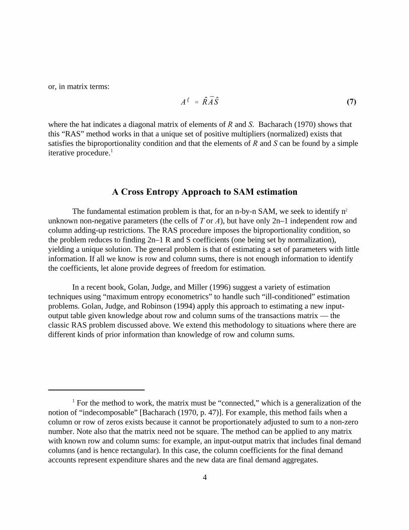
or, in matrix terms:

where the hat indicates a diagonal matrix of elements of R and S. Bacharach (1970) shows thatthis “RAS” method works in that a unique set of positive multipliers (normalized) exists thatsatisfies the biproportionality condition and that the elements of R and S can be found by a simpleiterative procedure. 1

A Cross Entropy Approach to SAM estimation

The fundamental estimation problem is that, for an n-by-n SAM, we seek to identify n2

unknown non-negative parameters (the cells of T or A), but have only 2n–1 independent row andcolumn adding-up restrictions. The RAS procedure imposes the biproportionality condition, sothe problem reduces to finding 2n–1 R and S coefficients (one being set by normalization),yielding a unique solution. The general problem is that of estimating a set of parameters with littleinformation. If all we know is row and column sums, there is not enough information to identifythe coefficients, let alone provide degrees of freedom for estimation.

In a recent book, Golan, Judge, and Miller (1996) suggest a variety of estimationtechniques using “maximum entropy econometrics” to handle such “ill-conditioned” estimationproblems. Golan, Judge, and Robinson (1994) apply this approach to estimating a new input-output table given knowledge about row and column sums of the transactions matrix — theclassic RAS problem discussed above. We extend this methodology to situations where there aredifferent kinds of prior information than knowledge of row and column sums.

& lnpi

qi

' & lnpi & lnqi

& I (p:q) ' &jn

i'1pi ln

pi

qi

Kapur and Kenavasan, 1992 presents a description of the axiomatic approach from which2

this measure is obtained (Chapter 4).

If the prior distribution is uniform, representing total ignorance, the method is equivalent3

to the “Maximum Entropy” estimation criterion (see Kapur and Kesavan, 1992; pp. 151-161).

5

(8)

(9)

Deterministic Approach: Information Theory

The estimation philosophy adopted in this paper is to use all, and only, the informationavailable for the estimation problem at hand. The first step we take in this section is to define whatis meant by “information”. We then describe the kinds of information that can be incorporated andhow to do it. This section focuses on information concerning non-stochastic variables while thenext section will introduce the use of information on stochastic variables.

The starting point for the cross entropy approach is Information Theory as developed byShannon (1948). Theil (1967) brought this approach to economics. Consider a set of n eventsE ,E , …,E with probabilities q , q ,…, q (prior probabilities). A message comes in which1 2 n 1 2 n

implies that the odds have changed, transforming the prior probabilities into posterior probabilitiesp , p ,…, p . Suppose for a moment that the message confines itself to one event E . Following1 2 n i

Shannon, the “information” received with the message is equal to -ln p . However, each E has itsi i

own posterior probability q , and the “additional” information from p is given by: i i

Taking the expectation of the separate information values, we find that the expected informationvalue of a message (or of data in a more general context) is

where I(p:q) is the Kullback-Leibler (1951) measure of the “cross entropy” distance between twoprobability distributions (Kapur and Kenavasan, 1992). The objective of the approach, which2

aims at utilizing all available information, is to minimize the cross entropy between theprobabilities that are consistent with the information in the data and the prior information q.3

Golan, Judge, and Robinson (1994) use a cross entropy formulation to estimate thecoefficients in an input-output table. They set up the problem as finding a new set of A

min jij

jAi,j ln

Ai,j

Ai,j

subject to jj

Ai,j y (

j ' y (

i

jj

Aj,i ' 1

0 # Aj,i # 1

Aij'Aij exp(8i y

(

j )

ji,j

Aijexp(8i y(

j )

A

AijAij

Although the CE method can be applied to SAM coefficients, one must take care when4

interpreting the resulting statistics because the parameters being estimated are no longerprobabilities, although the column coefficients satisfy the same axioms.

The problem has to be solved numerically because no closed form solution exists.5

6

(10)

(11)

(12)

(13)

coefficients which minimizes the entropy distance between the prior and the new estimatedcoefficient matrix. 4

The solution is obtained by setting up the Lagrangian for the above problem and solving it. The5

outcome combines the information from the data and the prior:

where 8 are the Lagrange multipliers associated with the information on row and column sums,i

and the denominator is a normalization factor.

The expression is analogous to Bayes’ Theorem, whereby the posterior distribution ( )is equal to the product of the prior distribution ( ) and the likelihood function (probability ofdrawing the data given parameters we are estimating), dividing by a normalization factor toconvert relative probabilities into absolute ones. The analogy to Bayesian estimation is that theapproach can be seen as an efficient Information Processing Rule (IPR) whereby we useadditional information to revise an initial set of estimates (Zellner, 1988, 1990). In this approachan “efficient” estimator is defined by Jaynes: “An acceptable inference procedure should have the

jij

jG (k)

i,j Ti,j ' ((k)

A

A

7

(14)

property that it neither ignores any of the input information nor injects any false information.”Zellner (1988) describes this as the “Information Conservation Principle.”

Types of Information

Priors The matrix from an earlier year provides information about the new coefficients. Theapproach is to estimate a new set of coefficients “close” to the prior.

Moment Constraints The most common kind of information to have is data on some or all of therow and column sums of the new SAM. This knowledge can be incorporated easily in the crossentropy framework by imposing a fixed value on y* in equation (11) in the same way as the RASmethod (eq. (5)). While the RAS procedure is based on knowing all row and column sums, it isonly one of several possible sources of information in CE estimation.

Economic Aggregates In addition to row and column sums, one often has additional knowledgeabout the new SAM. For example, aggregate national accounts data may be available for variousmacro aggregates such as value added, consumption, investment, government, exports, andimports. There also may be information about some of the SAM accounts such as governmentreceipts and expenditures. This information can be summarized as additional linear adding-upconstraints on various elements of the SAM. Define an n-by-n aggregator matrix, G, which hasones for cells in the aggregate and zeros otherwise. Assume that there are k such aggregationconstraints, which are given by:

where ( is the value of the aggregate. These conditions are simply added to the constraint set inthe cross entropy formulation. The conditions are linear in the coefficients and can be seen asadditional moment constraints.

Inequality Constraints While one may not have exact knowledge about values for variousaggregates, including row and column sums, it may be possible to put bounds on some of theseaggregates. Such bounds are easily incorporated by specifying inequality constraints in equations(11) and (14).

Stochastic Approach: Measurement Error

Most applications of economic models to real world issues must deal with the problem ofextracting results from data or economic relationships with noise. In this section we generalizeour approach to cases where: (i) row and column sums are not fixed parameters but involve errorsin measurement, and (ii) the initial estimate, , is not based on a balanced SAM.

Consider the standard regression model:

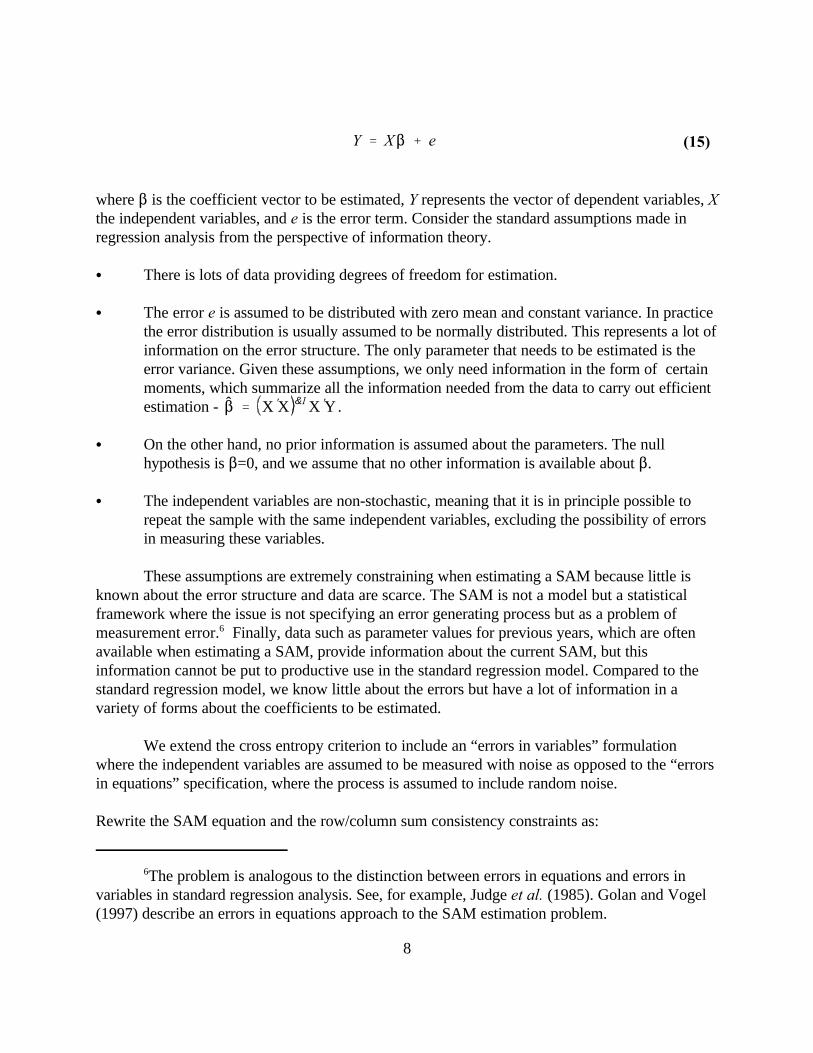
Y ' X$ % e

$ ' X 'X &1 X 'Y

The problem is analogous to the distinction between errors in equations and errors in6

variables in standard regression analysis. See, for example, Judge et al. (1985). Golan and Vogel(1997) describe an errors in equations approach to the SAM estimation problem.

8

(15)

where $ is the coefficient vector to be estimated, Y represents the vector of dependent variables, Xthe independent variables, and e is the error term. Consider the standard assumptions made inregression analysis from the perspective of information theory.

C There is lots of data providing degrees of freedom for estimation.

C The error e is assumed to be distributed with zero mean and constant variance. In practicethe error distribution is usually assumed to be normally distributed. This represents a lot ofinformation on the error structure. The only parameter that needs to be estimated is theerror variance. Given these assumptions, we only need information in the form of certainmoments, which summarize all the information needed from the data to carry out efficientestimation - .

C On the other hand, no prior information is assumed about the parameters. The nullhypothesis is $=0, and we assume that no other information is available about $.

C The independent variables are non-stochastic, meaning that it is in principle possible torepeat the sample with the same independent variables, excluding the possibility of errorsin measuring these variables.

These assumptions are extremely constraining when estimating a SAM because little isknown about the error structure and data are scarce. The SAM is not a model but a statisticalframework where the issue is not specifying an error generating process but as a problem ofmeasurement error. Finally, data such as parameter values for previous years, which are often6

available when estimating a SAM, provide information about the current SAM, but thisinformation cannot be put to productive use in the standard regression model. Compared to thestandard regression model, we know little about the errors but have a lot of information in avariety of forms about the coefficients to be estimated.

We extend the cross entropy criterion to include an “errors in variables” formulationwhere the independent variables are assumed to be measured with noise as opposed to the “errorsin equations” specification, where the process is assumed to include random noise.

Rewrite the SAM equation and the row/column sum consistency constraints as:

y ' A x % e ' Ax % A e

y ' x % e

ei ' jw

Wi,w vi,w

jw

Wi,w ' 1

and 0 # Wi,w #1

ei ' Wi vi & (1 & Wi) vi

9

(16)

(17)

(18)

(19)

where y is the vector of row sums and x, measured with error e, is the initial known vector ofcolumn sums. Following Golan, Judge, and Miller (1994, chapter 6), we write the errors as aweighted average of known constants as follows:

subject to the weights summing to one:

where w is the set of weights, W. In the estimation, the weights are treated as probabilities to beestimated. The constants, <, define the “support” set for the errors and are usually chosen to yielda symmetric distribution with moments depending on the number of elements in the set w. Forexample, if the error distribution is assumed to be rectangular and symmetric around zero, withknown upper and lower bounds, the error equation becomes:

In this case the variance is fixed. In general, one can add more v’s and W's to incorporate moreinformation about the error distribution (e.g., more moments, including variance, skewness, andkurtosis).

Given knowledge about the error bounds, equations (17) and (18) are added to theconstraint set and equation (16) replaces the SAM equation (equation 3). The problem is messierin that the SAM equation is now nonlinear, involving the product of A and e. The minimizationproblem is to find a set of A’s and W’s that minimize cross entropy including a term in the errors:

min jij

jAi,j ln Ai,j & j

ij

jAi,j ln Ai,j % j

i[ Wi ln Wi % (1 & Wi ) ln 1

2]

I A,W : A ' jij

jAi, j ln Ai, j & j

ij

jAi, j ln Ai, j

% jij

wWi,w ln Wi,w & j

ij

wWi,w ln 1

n

A

When the error distribution is assumed to be rectangular between the upper and lower7

bounds, and is symmetric around zero (that is only two W’s), equation (20) is written as:

Arndt, C. et al. (1997) describe the Mozambique SAM in detail.8

10

(20)

subject to the constraint equations that column and row sums be equal, and that the W’s and A’'sfall between zero and one, and any other linear known aggregation inequalities or equalities(where n is the number of elements in the set W,). Note that if the distribution is symmetric, thenwhen all the W’s are equal, which is the default prior, all the errors are zero. 7

We are minimizing equation 20 over the A’s (SAM coefficients) and W’s (weights on theerror term), where the W’s are treated like the A’s. In the estimation procedure, the termsinvolving the A’s and W’s are assigned equal weights, reflecting an equal preference for“precision” (the A’s) in the estimates of the parameters, and “prediction” (the W’s) or the“goodness of fit” of the equation on row and column sums. Golan, Judge, and Miller (1996)report Monte Carlo experiments where they explore the implications of changing these weightsand conclude that equal weighting of precision and prediction is reasonable.

Another source of measurement error may arise if the initial SAM, , is not itself abalanced SAM. That is, its corresponding rows and columns may not be equal. This situation doesnot change the cross entropy estimation procedure, but implies that it is not possible to achieve across entropy measure of zero because the prior is not feasible. The idea is to find a new feasibleSAM that is “entropy-close” to the infeasible prior.

An Example: Mozambique

To illustrate the use of the proposed cross entropy estimator, we apply it to recover analready existing 1994 macro SAM for Mozambique (Table 3). The original SAM is perturbed to8

be inconsistent, with some row and column sums not equal (Table 4). Starting from the perturbedinconsistent SAM as our prior, the problem is to estimate the coefficients of the original SAM.

11

We report the results and the efficiency gains from adding information to the estimation problem.The gains are evaluated according to how close the estimated SAM is to the initial SAM — theSAM in Table 3.

Three estimation results are reported. The first set of “Core” results are estimated underthe assumption of no information and uses the core cross entropy method where only equations(11) and (12) are imposed as constraints (or equivalently, equations 1-8 in Appendix A with allerror terms set to zero). The second set (Allfix) adds additional information assumed known fromother sources. The additional information includes moment constraints on some row and columnsums, inequality constraints, and knowledge of various economic aggregates like totalconsumption, exports, imports, and GDP at market prices. The third (Allfix plus error) extendsthe second estimation method to include the “errors in variables” formulation, adding informationon additional row and column sums assumed to be measured with error. For the error term (e ),i

we specify an error support set with three elements centered on zero, allowing a two-parametersymmetric distribution with unknown variance.

For each SAM estimation, Tables 5-7 report the new estimated balanced SAM along withthe cell-by-cell deviation from the initial SAM. In addition, a set of estimation statistics relevant toeach estimated SAM are reported in Table 2, which indicates the gains from adding information tothe estimation problem.

Table 2. Estimation statistics

Core AllFix Allfix plus error

Root Mean Square Error (RMSE) 2.4718 0.9406 0.7785

Coefficient RMSE 0.0112 0.0110 0.0072

CE associated with SAM coefficients 0.0000 0.0007 0.0028*

CE associated with error term 0.0000 0.0000 0.0010

Total CE 0.0000 0.0007 0.0038

Note: Core = estimation under the assumption of no information added. AllFix = estimation with additional information (moment constraints on some row and column sums, aggregate economic data on total consumption, exports, imports, and GDP at marketprices). AllFix plus error = AllFix + “errors in variables” formulation on remaining column sums.* CE = cross entropy

The gains from adding information to the estimation problem are evaluated according tohow close the estimated SAM is to the initial SAM, in terms of both flows and coefficients. FromTable 2, the root mean square error (RMSE) for the SAM flows and the SAM coefficients,measured relative to the initial SAM, falls as we add more information to the Core estimation. A

Ay ' y

The CE measure associated with the error term is zero for the Core and AllFix cases9

because the error term is set to zero and the column totals are free to vary, so no constraint isimposed.

12

falling RMSE indicates that the estimated SAM coefficients have a smaller dispersion around theirrespective true values (represented by the initial SAM).

The Cross-Entropy measures reflect how much the information we have introduced hasshifted our solution away from the inconsistent prior, and also accounting for the imprecision ofthe moments assumed to be measured with error. Intuition suggests that if the informationconstraints are binding the distance from the prior will increase; if none are binding then the crossentropy (CE) distance will be zero. That is, there exists a y, such that . In our Core casewithout any constraints on the y other than that column and row sums must be equal, a solutioncan be found without changing the column coefficients, as indicated by a CE measure of zero.9

We observe that, as more information is imposed, the CE measure increases as expected.

In the final estimation (AllFix with error), we impose a full set of column sums(information on y), but some are assumed to be measured with error. We end up with a CEmeasure associated with the error term that is larger, but the RMSE is smaller. The addedinformation is significantly improving our estimate even when information is added in an impreciseway. The RMSE in Table 2 falls significantly as more information is used — by about 66 percentfor the AllFix, and an additional 20 percent for the final estimation.

Conclusion

The cross entropy approach provides a flexible and powerful method for estimating asocial accounting matrix (SAM) when dealing with scattered and inconsistent data. The methodrepresents a considerable extension of the standard RAS method, which assumes that one startsfrom a consistent prior SAM and has knowledge only about row and column totals. The crossentropy framework allows a wide range of prior information to be used efficiently in estimation.The prior information can be in a variety of forms, including linear and nonlinear inequalities,errors in equations, measurement error (using an error-in-variables formulation). One also neednot start from a balanced or consistent SAM. We have presented cross entropy estimation resultsapplied to the case of a SAM for Mozambique, where we started from a perturbed inconsistentSAM as our prior. Then we measured the gains from incorporating a wide range of informationfrom a variety of sources to improve our estimation of the SAM parameters.

13

Table 3. Initial balanced 1994 Macro SAM for Mozambique (millions of 1994 meticais)

Expenditure

Receipts (1) (2) (3) (4) (5) (6) (7) (8) (9) (10) (11) (12) Totals

(1) Agr. activity 25.14 30.49 55.63

(2) Non-agr. activity 12.46 206.28 2.14 220.88

(3) Agr. Commodity 1.58 13.42 20.12 0.00 0.09 8.58 43.79

(4) Non-agr. Commodity 7.24 98.86 86.72 16.78 0.00 33.94 33.03 24.13 300.69

(5) Factors 47.01 108.74 155.75

(6) Enterprises 62.86 62.86

(7) Households 91.63 58.96 1.33 3.46 155.38

(8) Rec. govt.* 0.94 9.88 1.26 2.41 2.48 5.55 22.53

(9) Indirect tax -0.19 -0.14 0.24 5.64 5.55

(10) Govt. investment 22.94 22.94

(11) Private investment 1.49 13.42 4.43 -11.00 24.79 33.12

(12) Rest of the world 5.01 78.89 83.90

Totals 55.63 220.88 43.79 300.69 155.75 62.86 155.38 22.53 5.55 22.94 33.12 83.90 1163.02

Source: Arndt, C. et al., 1997.* Recurrent government expenditures

14

Table 4. Perturbed unbalanced 1994 Macro SAM for Mozambique (millions of 1994 meticais)

Expenditure

Receipts (1) (2) (3) (4) (5) (6) (7) (8) (9) (10) (11) (12) Totals

(1) Agr. activity 20.00 30.49 50.49(-5.14) (-5.14)

(2) Non-agr. activity 12.46 195.00 2.14 209.60(-11.28) (-11.28)

(3) Agr. Commodity 1.58 13.00 20.12 0.00 0.09 8.58 43.37(-0.42) (-0.42)

(4) Non-agr. Commodity 7.24 96.00 86.72 16.78 0.00 32.00 35.00 24.13 297.86(-2.86) (-1.94) (-1.97) (-2.82)

(5) Factors 47.01 108.74 155.75

(6) Enterprises 62.86 62.86

(7) Households 91.63 60.00 1.33 3.46 156.42(-1.04) (1.04)

(8) Rec. govt.* 0.94 9.88 1.26 2.41 2.48 5.55 22.53

(9) Indirect tax -0.19 -0.14 0.24 5.64 5.55

(10) Govt. investment 22.94 22.94

(11) Private investment 1.49 12.00 4.43 -11.00 24.79 31.70(-1.42) (-1.42)

(12) Rest of the world 5.01 78.89 83.90

Totals 55.63 217.60 38.65 289.41 155.75 63.90 153.96 22.53 5.55 21.00 35.09 83.90 1163.02(-3.27) (-11.28) (-1.04) (-1.42) (-1.94) (-1.97)

Source: Arndt, C. et al., 1997.* Recurrent government expenditures Note: numbers in parenthesis represent the difference between the perturbed SAM and the true SAM of Table 3.

15

Table 5. Core Cross Entropy estimation for the 1994 Macro SAM for Mozambique (Core) (millions of 1994 meticais)

Expenditure

Receipts (1) (2) (3) (4) (5) (6) (7) (8) (9) (10) (11) (12) Totals

(1) Agr. activity 21.77 29.36 0.00 51.13(-3.37) (-1.14) (-4.50)

(2) Non-agr. activity 13.57 194.63 2.06 0.00 210.26(1.11) (-11.65) (-0.08) (-10.62)

(3) Agr. Commodity 1.45 12.56 19.37 0.00 0.09 8.61 42.08(-0.13) (-0.86) (-0.75) (-0.01) (0.03) (-1.71)

(4) Non-agr. Commodity 6.65 92.76 83.49 16.61 0.00 33.09 32.04 24.22 288.86(-0.58) (-6.09) (-3.23) (-0.17) (-0.85) (-0.98) (0.08) (-11.82)

(5) Factors 43.22 105.07 148.29(-3.79) (-3.67) (-7.46)

(6) Enterprises 59.85 59.85(-3.01) (-3.01)

(7) Households 87.24 56.20 1.32 3.47 148.22(-4.39) (-2.76) (-0.01) (0.01) (-7.15)

(8) Rec. govt.* 1.02 9.87 1.20 2.26 2.39 5.56 22.30(0.08) (-0.02) (-0.06) (-0.15) (-0.09) (0.01) (-0.23)

(9) Indirect tax -0.19 -0.14 0.26 5.63 5.56(0.02) (-0.01) (0.01)

(10) Govt. investment -0.93 23.02 22.09(-0.92) (0.08) (-0.85)

(11) Private investment 1.39 11.55 4.38 -11.00 24.88 31.20(-0.09) (-1.87) (-0.05) (0.09) (-1.92)

(12) Rest of the world 5.45 78.74 84.19(0.44) (-0.15) (0.29)

Totals 51.13 210.26 42.08 288.86 148.29 59.85 148.22 22.30 5.56 22.09 31.20 84.19(-4.50) (-10.62) (-1.71) (-11.82) (-7.46) (-3.01) (-7.15) (-0.23) (0.01) (-0.85) (-1.92) (0.29)

Source: Arndt, C. et al., 1997.* Recurrent government expenditures Note: numbers in parenthesis represent the difference between the estimated SAM and the initial SAM of Table 3.

16

Table 6. Cross Entropy and additional information estimation for the 1994 Macro SAM for Mozambique (AllFix) (millions of 1994 meticais)

Expenditure

Receipts (1) (2) (3) (4) (5) (6) (7) (8) (9) (10) (11) (12) Totals

(1) Agr. activity 22.52 30.77 0.00 53.29(-2.62) (0.28) (-2.34)

(2) Non-agr. activity 14.02 203.10 2.15 0.00 219.27(1.55) (-3.17) (0.01) (-1.61)

(3) Agr. Commodity 1.51 13.07 20.17 0.00 0.09 8.60 43.45(-0.07) (-0.35) (0.05) (0.02) (-0.35)

(4) Non-agr. Commodity 6.90 95.65 86.38 16.79 0.00 33.52 33.44 24.11 296.79(0.33) (-3.20) (-0.34) (0.01) (-0.42) (0.41) (-0.02) (-3.89)

(5) Factors 45.07 110.68 155.75(-1.94) (1.94)

(6) Enterprises 62.94 62.94(0.08) (0.08)

(7) Households 91.54 59.05 1.31 3.31 155.21(-0.08) (0.09) (-0.01) (-0.15) (-0.17)

(8) Rec. govt.* 1.05 9.78 1.27 2.38 2.52 5.55 22.53(0.11) (-0.11) (-0.03) (0.03)

(9) Indirect tax -0.19 -0.14 0.27 5.61 5.55(0.03) (-0.03)

(10) Govt. investment -0.49 23.01 22.52(-0.49) (0.07) (-0.42)

(11) Private investment 1.52 13.22 4.43 -11.00 24.87 33.04(0.03) (-0.20) (0.08) (-0.09)

(12) Rest of the world 5.59 78.31 83.90(0.58) (-0.58)

Totals 53.29 219.27 43.45 296.79 155.75 62.94 155.21 22.53 5.55 22.52 33.04 83.90(-2.34) (-1.61) (-0.35) (-3.89) (0.08) (-0.17) (-0.42) (-0.09)

Source: Arndt, C. et al., 1997.* Recurrent government expenditures Note: numbers in parenthesis represent the difference between the estimated SAM and the initial SAM of Table 3.

17

Table 7. Cross Entropy and additional column sums measured with error estimation for the 1994 Macro SAM for Mozambique (AllFix plus error) (millions of 1994meticais)

Expenditure

Receipts (1) (2) (3) (4) (5) (6) (7) (8) (9) (10) (11) (12) Totals

(1) Agr. activity 23.36 32.26 0.00 55.62(-1.78) (1.77)

(2) Non-agr. activity 13.40 202.98 1.68 0.00 218.06(0.94) (-3.30) (-0.46)

(3) Agr. Commodity 1.58 13.14 19.96 0.00 0.09 8.60 43.37(-0.28) (-0.16) (0.02)

(4) Non-agr. Commodity 7.24 96.30 85.57 16.64 0.00 33.93 33.18 24.11 296.97(-2.55) (-1.15) (-0.14) (-0.01) (0.16) (-0.02)

(5) Factors 47.00 108.76 155.75(-0.02) (0.02)

(6) Enterprises 62.86 62.86

(7) Households 91.61 58.95 1.35 3.30 155.21(-0.02) (-0.01) (0.02) (-0.16)

(8) Rec. govt.* 1.01 9.82 1.28 2.39 2.50 5.54 22.53(0.06) (-0.06) (0.02) (-0.03) (0.01)

(9) Indirect tax -0.19 -0.14 0.26 5.62 5.55(0.02) (-0.02)

(10) Govt. investment 0.11 22.82 22.93(-0.12)

(11) Private investment 1.52 13.24 4.55 -11.00 25.07 33.38(0.04) (-0.18) (0.13) (0.28)

(12) Rest of the world 5.35 78.55 83.90(0.34) (-0.34)

Totals 55.62 218.06 43.37 296.97 155.75 62.86 155.21 22.53 5.55 22.93 33.38 83.90(-0.02) (-2.81) (-0.42) (-3.71) (0.00) (-0.17) (-0.01) (0.26)

Source: Arndt, C. et al., 1997.* Recurrent government expenditures Note: numbers in parenthesis represent the difference between the estimated SAM and the initial SAM of Table 3.

18

References

Arndt, C., A. Cruz, H. Jensen, S. Robinson, and F. Tarp. 1997. A social accounting matrix forMozambique: Base Year 1994. Institute of Economics, University of Copenhagen.

Bacharach, M. 1970. Biproportional Matrices and Input-Output Change. CambridgeUniversity Press. University of Cambridge, Department of Applied Economics.

Brooke, A., D. Kendrick, and A. Meeraus. 1988. GAMS a User's Guide, San Francisco: TheScientific Press.

Golan, A., G. Judge, and D. Miller. 1996. Maximum Entropy Econometrics, Robust Estimationwith Limited Data. John Wiley & Sons.

Golan, A., G. Judge, and S. Robinson. 1994. Recovering information from incomplete or partialmultisectoral economic data. Review of Economics and Statistics 76, 541-9.

Golan, A., and S. J. Vogel. 1997. Estimation of stationary and non-stationary accounting matrixcoefficients with structural and supply-side information. ERS/USDA. Unpublished.

Judge, G.G. et al. 1985. The Theory and Practice of Econometrics. John Wiley & Sons.

Kapur, J.N and H.K. Kesavan. 1992. Entropy Optimization Principles with Applications.Academic Press.

Kullback, S. and R.A. Leibler. 1951. On information and sufficiency. Ann. Math. Stat. 4, 99-111.

Pindyck, R.S., and D.L. Rubinfeld. 1991. Econometric Models & Economic Forecasts. McGrawHill.

Shannon, C. E. 1948. A mathematical theory of communication. Bell System TechnicalJournal 27, 379-423.

Theil, H. 1967. Economics and Information Theory. Rand McNally.

Zellner, A. 1988. Optimal information processing and bayes theorem. American Statistician42, 278-84.

Zellner, A. 1990. Bayesian methods and entropy in economics and econometrics. In W. T.Grandy and L. H. Shick (Eds.), Maximum Entropy and Bayesian Methods, pp. 17-31.Kluwer, Dordrecht.

Appendix A: Mathematical Representation

I A,W : A ' jij

jAi, j ln Ai, j & j

ij

jAi, j ln Ai, j

% jij

wWi,w ln Wi,w & j

ijw

Wi,w ln 1n

Ti,j ' Ai,j ( Xi % ei )

Yi ' Xi % ei

ei ' jw

Wi,w vi,w

jj

Ti, j ' Xi % ei

ji

Ti, j ' Yj

ji

Ai, j ' 1 and 0< Ai, j<1

jw

Wi,w ' 1 and 0< Wi,w< 1

jij

jG (k)

i,j Ti,j ' ((k)

Ai, j

G (k)i,j

((k)

n

vi, jwt

Xi

20

Table A.1: Cross Entropy Equations

# Equation Description

1 Cross-Entropy minimand

2 SAM equation

3 Row/column sum consistency

4 Error definition

5 Row sum

6 Column sum

7 Sum of Column coefficients

8 Sum of weights on errors

9 Additional Constraints

Notation

Set Parameters

i and j SAM accountsw weights on error support set

VariablesA SAM coefficient matrixi,j

e Error variablei

I Cross Entropy measure(objective)

T Transactions SAMi,j

W Error weightsi, w

Y Row sumi

Prior SAM coefficient matrix

k’th aggregator matrix

k’th control total

number of elements in set w

Error support values, including

bounds

fixed value of column sum

Appendix B: GAMS Code

22

Appendix B: GAMS code

What follows is a listing of the GAMS program used in illustrating the entropy

difference method discussed above. A quick list of some of GAMS features are listed below. For

additional information about GAMS syntax see Brooke, Kendrick, and Meeraus (1988).

In the GAMS language:

- Parameters are treated as constants in the model and are defined in separate

"PARAMETER" statements.

- "SUM" is the summation operator, sigma.

- "$" introduces a conditional "if" statement.

- The suffix ".FX" indicates a fixed variable.

- The suffix ".L" indicates the level or solution value of a variable.

- The suffix ".LO" and ".UP" indicate the lower and upper bounds, respectively

of a variable.

- An asterisk "*" in the first column indicates a comment. Alternative treatments

in the model Code are shown commented out.

- An "ALIAS" statement is used to give another name to a previously declared set.

- A semicolon (;) terminates a GAMS statement.

- Items between slashes (/) are data or set elements.

23

$TITLE Entropy Difference. Mozambique Macro SAM *################################################################$OFFSYMLIST OFFSYMXREF OFFUPPER ####### *########################################################### SETS############** i macrosam accounts / AGRA Agricultural activities * MOZAM101 start by aggregating the balanced micro SAM NAGRA Non agricultural activities reported in: AGRC Agricultural Commodities * Arndt, Channing, et al. (1998) " Social Accounting Matrices for NAGRC Non agricultural Commodities * Mozambique 1994 and 1995" MERISSA projectworking paper No. XX FAC Factors * IFPRI, Washington, D.C. ENT Enterprises * The aggregated SAM is then perturbed and the Cross Entropy HOU Households Method GRE Govt recurrent expenditures * is used under different assumptions about data ITAX Indirect taxesavailability to GIN Govt investment * re-estimate it. CAP Capital account * ROW Rest of world * Programmed by Sherman Robinson, Andrea Cattaneo, andMoataz El-Said, TOTAL /* June 1998.* Trade and Macroeconomics Division* International Food Policy Research Institute (IFPRI) ii(i) all acounts in i except TOTAL * 2033 K St., N.W.* Washington, DC 20006 USA * For a uniform distribution, set jwt to only two entries. Error* Email: S.Robinson@CGIAR.ORG * range set below with the vbar parameter.* A.Cattaneo@CGIAR.ORG* M.El-Said@CGIAR.ORG jwt weights on errors in variables / 1*3 / ** Method described in S. Robinson and M. El Said, AA(i) activity /AGRA "Estimating a Social NAGRA / * Accounting Matrix Using Cross Entropy Methods." September1997. CC(i) Commodity /AGRC* See also A. Golan, G. Judge, and D. Miller, Entropy NAGRC /Difference* Econometrics, John Wiley & Sons, 1996. F(i) Factors /FAC /** Based on program used in C. Arndt, A. S. Cruz, H. T. H(i) Households /HOU /Jensen,* S. Robinson, and F. Tarp, "A Social Accounting Matrix for G(i) Government and Investment accounts /GREMozambique: ITAX* Base Year 1994." Institute of Economics, University of GINCopenhagen, CAP /* March 1997. * FIX(i) Accounts to be fixed when solving core with allfix* Original version programmed by Sherman Robinson and Andrea / FAC, GRE, ITAX, ROWCattaneo. /* ;

24

ii(i) = YES; 22.942ii("Total") = NO; CAP 13.422 4.426 -11.000

ALIAS (AA,AAP), (CC,CCP), (F,FP), (H,HP) ; TOTAL 155.377 22.534 5.546 22.942 33.121 ALIAS (i,j), (ii,jj); 83.899

*######################## SAM DATABASE ############################# AGRA 55.631*Initial balanced Macro SAM (aggregate of Micro SAM / NAGRA 220.879parameter SAM1) AGRC 43.792

Table SAM1(i,j) Social accounting matrix FAC 155.752

AGRA NAGRA AGRC NAGRC HOU 155.377FAC ENT GRE 22.534

AGRA 25.140 GIN 22.942NAGRA 12.464 206.275 CAP 33.121AGRC 1.578 13.419 ROW 83.899NAGRC 7.235 98.855 TOTAL 1163.020FAC 47.012 108.740 ;ENT 62.860 SAM1("TOTAL",jj) = sum(ii, SAM1(ii,jj));HOU SAM1(ii,"TOTAL") = sum(jj, SAM1(ii,jj));91.629 58.961GRE 0.941 9.885 1.263 2.414 *######################### Parameters and ScalarsITAX -0.194 -0.135 0.239 5.636 ########################CAP PARAMETER 1.485ROW 5.007 78.892 SAM(i,j) Base SAM transactions matrix (in 100 bn. ofTOTAL 55.631 220.879 43.792 300.687 1995 Meticais)155.752 62.860 SAM0(i,j) Base SAM transactions matrix (used for

+ HOU GRE ITAX GIN SAM2(i,j) Base perturbed SAM transactions matrix (usedCAP ROW for comparison)

AGRA 30.491 PERCENT(i,j) Percent change of SAM from SAM0NAGRA 2.140 T0(i,j) Matrix of SAM transactions (flow matrix)AGRC 20.120 -2.40000E-4 T00(i,j) Matrix of SAM transactions (flow matrix)0.095 8.581 T1(i,j) Adjusted matrix of SAM transactions forNAGRC 86.720 16.778 -2.20000E-4 33.942 negative coefficients33.027 24.131 T2(i,j) Adjusted original matrix of SAM transact forHOU 1.331 (-)ve coefficients 3.457 Abar0(i,j) Prior SAM coefficient matrix GRE 2.485 5.547 Abar1(i,j) Adjusted prior SAM coefficient matrix for

GIN

24.789

+ TOTAL

NAGRC 300.687

ENT 62.860

ITAX 5.546

comparison reports)

DIFF(i,j) Difference between SAM and SAM0

negative coefficients

25

Abar00(i,j) Prior SAM coefficient matrix Abar11(i,j) Adjusted prior SAM coefficient matrix for SAM2(i,j) = SAM(i,j);negative coefficients DIFF(i,j) = SAM(i,j) - SAM0(i,j) ; Target0(i) Targets for macro SAM column totals PERCENT(i,j)$SAM(i,j) = 100*(SAM(i,j) - SAM0(i,j))/SAM0(i,j); Vbar(i,jwt) Error bounds DELTA Tolerance to allow zero entries in new SAM; Display SAM, SAM0, DIFF, PERCENT;

SCALARS *################# Divide SAM entries by 10 for better scaling

sumtarg0 sum of targets SAM(i,j) = sam(i,j)/10; TM0 Total imports SAM1(i,j) = sam1(i,j)/10; TX0 Total exports TC0 Total household consumption *################# Initializing Parameters TVA0 total value added from true SAM GDPMP0 GDP at market prices Abar0(ii,jj)$SAM(ii,jj) = SAM(ii,jj)/SAM("TOTAL",jj) ;

; *############ Setting SAM to aggregated SAM1 then perturbing T0(ii,jj) = SAM(ii,jj);it ############ T0("TOTAL",jj) = SUM(ii, SAM(ii,jj));

SAM(i,j) = SAM1(i,j); SAM0(i,j) = SAM(i,j); T00(ii,jj) = SAM1(ii,jj);

* Perturbing Domestic sales T00(ii,"TOTAL") = SUM(jj, SAM(ii,jj)); SAM("AGRA","AGRC") = 20.00; SAM("NAGRA","NAGRC") = 195.00; DELTA = .000001;

* Perturbing Intermediate demand Display T0, Abar0, sam0 ; SAM("AGRC","NAGRA") = 13.00; SAM("NAGRC","NAGRA") = 96.00; *######################## CROSS ENTROPY

* Perturbing Enterprise payment to Household SAM("HOU","ENT") = 60.00;

* Perturbing Household Savings ############################### SAM("CAP","HOU") = 12.00; * The ENTROPY DIFFERENCE procedure uses LOGARITHMS: negative* Perturbing Government investment (Gov't Investment to flows incommodities) * the SAM are NOT GOOD!!! SAM("NAGRC","GIN") = 32.00; *

* Perturbing investment (Capital payment to commodities) them out SAM("NAGRC","CAP") = 35.00; * of their respective symmetric cells, e.g.

* ############## calculating totals * and ADDED to GRE ---> ACT as a positive number.

SAM("TOTAL",jj) = sum(ii, SAM(ii,jj)); * After balancing, the negative SAM values are returned to theirSAM(ii,"TOTAL") = sum(jj, SAM(ii,jj)); * original cells for printing.

Abar00(ii,jj)$SAM1(ii,jj) = SAM1(ii,jj)/SAM1("TOTAL",jj) ;

T0(ii,"TOTAL") = SUM(jj, SAM(ii,jj));

T00("TOTAL",jj) = SUM(ii, SAM(ii,jj));

###############################

*######################## RED ALERT!!!

* The option used here is to detect any negative flows and net

* negative flow ACT ---> GRE is set to zero

* The entropy difference method can then be implemented.

26

SET red(i,j) Set of negative SAM flows redsam1("total",jj) = sum(ii, redsam1(ii,jj)); ; redsam1(ii,"total") = sum(jj, redsam1(ii,jj));

Parameter sam(ii,"total") = sum(jj, T1(ii,jj)); redsam(i,j) Negative SAM values only sam("total",jj) = sum(ii, T1(ii,jj)); rtot(i) Row total ctot(i) Column total sam1(ii,"total") = sum(jj, T2(ii,jj));

redsam1(i,j) Negative SAM values only rtot1(i) Row total rtot(ii) = sum(jj, T1(ii,jj)); ctot1(i) Column total ctot(jj) = sum(ii, T1(ii,jj));

; rtot1(ii) = sum(jj, T2(ii,jj));

rtot(ii) = sum(jj, T0(ii,jj)); ctot(jj) = sum(ii, T0(ii,jj)); Abar1(ii,jj) = T1(ii,jj)/sam("total",jj); rtot1(ii) = sum(jj, T00(ii,jj)); Abar11(ii,jj) = ctot1(jj) = sum(ii, T00(ii,jj)); T2(ii,jj)/sam1("total",jj);

red(ii,jj)$(T0(ii,jj) LT 0) = yes ; display "NON-NEGATIVE SAM" ; redsam(ii,jj) = 0; display redsam, T1, T2, Abar0, Abar1, rtot, ctot ; redsam(ii,jj)$red(ii,jj) = T0(ii,jj); redsam(jj,ii)$red(ii,jj) = T0(ii,jj);

red(ii,jj)$(T00(ii,jj) LT 0) = yes ; values ####### redsam1(ii,jj) = 0; *SR Note that target column sums are being set to average of redsam1(ii,jj)$red(ii,jj) = T00(ii,jj); initial redsam1(jj,ii)$red(ii,jj) = T00(ii,jj); * row and column sums. Initial column sums could have been used

*Note that redsam includes each entry twice, incorresponding row target0(ii) = (sam(ii,"total") + sam("total",ii))/2 ;*and column. So, redsam need only be subtracted from T0. target0(aa) = sam("total",aa) ; T1(ii,jj) = T0(ii,jj) - target0(cc) = sam(cc,"total") ;redsam(ii,jj); target0("ent") = sam("ent","total") ; T1("Total",jj) = sum(ii, T1(ii,jj)); target0("gin") = sam("gin","total") ; T1(ii,"Total") = sum(jj, T1(ii,jj)); sumtarg0 = sum(ii, sam(ii,"total") );

T2(ii,jj) = T00(ii,jj) - TX0 = SUM(CC, T2(CC,"ROW"));redsam1(ii,jj); TVA0 = T2("FAC","AGRA") + T2("FAC","NAGRA"); T2("Total",jj) = sum(ii, T2(ii,jj)); TC0 = SUM((AA,H), T2(AA,H)) + SUM((CC,H), T2(ii,"Total") = sum(jj, T2(ii,jj)); T2(CC,H));

redsam("total",jj) = sum(ii, Display TVA0, TC0, TX0, TM0, GDPMP0;redsam(ii,jj)); *###################### VARIABLES

redsam(ii,"total") = sum(jj, redsam(ii,jj));

sam1("total",jj) = sum(ii, T2(ii,jj));

ctot1(jj) = sum(ii, T2(ii,jj));

*##### Initializing Parameters after accounting for negative

instead,* depending on data quality and prior knowledge.

TM0 = SUM(CC, T2("ROW",CC));

GDPMP0 = TC0 + TX0 + SUM((CC,G), T2(CC,G)) - TM0;

########################################

27

VARIABLES *############ EQUATIONS IMPOSING KNOWN INFORMATION A(i,j) Post SAM coefficient matrix TSAM(i,j) Post matrix of SAM transactions TOTVA Total value added is known Y(i) row sum of SAM TOTC Total Consumption X(i) column sum of SAM TOTX Total exports ERR(i) Error value TOTM Total Imports W(i,jwt) Error weight TOTGDP GDP at market prices DENTROPY Entropy difference (objective) ; TVA Total value added or GDP at factor cost TC Total consumption *CORE TX Total exports EQUATIONS====================================================== TM Total imports GDPMP GDP at market prices

;

*########################## INITIALIZE VARIABLES TSAM(ii,jj) =E= A(ii,jj) * (X(jj) + ERR(jj)) ;##########################

A.L(ii,jj) = Abar1(ii,jj) ; W(ii,jwt)*vbar(ii,jwt)) ; TSAM.l(ii,jj) = T1(ii,jj); Y.L(ii) = target0(ii) ; SUMW(ii).. SUM(jwt, W(ii,jwt)) =E= 1 ; X.L(ii) = target0(ii) ; ERR.L(ii) = 0.0 ; ENTROPY.. DENTROPY =E= SUM((ii,jj)$(Abar1(ii,jj)), W.L(ii,jwt) = 1/card(jwt) ; A(ii,jj)*(LOG(A(ii,jj) + delta) DENTROPY.L = 0; - LOG(Abar1(ii,jj) + delta))) TVA.L = TVA0; + SUM((ii,jwt), W(ii,jwt) TC.L = TC0; * (LOG(W(ii,jwt) + delta) TX.L = TX0; - LOG((1/card(jwt)) + delta)) ) TM.L = TM0; ; GDPMP.L = GDPMP0; ROWSUM(ii).. SUM(jj, TSAM(ii,jj)) =E= Y(ii) ;Display TM.l; COLSUM(jj).. SUM(ii, TSAM(ii,jj)) =E= (X(jj) + ERR(jj)) ;*############ CORE EQUATIONS EQUATIONS COLSUM2(jj).. SUM(ii, A(ii,jj)) =E= 1;

SAMEQ(i) row and column sum constraint *ADDITIONAL MACRO CONTROL-TOTAL SAMMAKE(i,j) make SAM flows EQUATIONS=========================== ERROREQ(i) definition of error term SUMW(i) Sum of weights TOTVA.. TVA =E= TSAM("FAC","AGRA") + ENTROPY Entropy difference definition TSAM("FAC","NAGRA"); ROWSUM(i) row target COLSUM(j) column target TOTC.. TC =E= SUM((AA,H), TSAM(AA,H)) COLSUM2(j) column coefficients + SUM((CC,H), TSAM(CC,H));

SAMEQ(ii).. Y(ii) =E= X(ii) + ERR(ii) ;

SAMMAKE(ii,jj)$(Abar1(ii,jj))..

ERROREQ(ii).. ERR(ii) =E= SUM(jwt,

TOTX.. TX =E= SUM(CC, TSAM(CC,"ROW"));

28

TOTM.. TM =E= SUM(CC, TSAM("ROW",CC)); vbar(ii,"1") = .10*target0(ii) ;

TOTGDP.. GDPMP =E= TC + TX + SUM((CC,G), vbar(fix,"1") = .0*target0(fix) ;TSAM(CC,G)) - TM; vbar(fix,"3") = .0*target0(fix) ;

*################ Defining bounds for cell values *SR to use only two weights, delete set element "2" in jwt and ######################## *comment out next statement.

A.LO(ii,jj)$ABAR1(ii,jj) = 0 ; W.LO(ii,jwt) = 0 ; A.UP(ii,jj)$ABAR1(ii,jj) = 1 ; W.UP(ii,jwt) = 1 ; A.FX(i,j)$(NOT Abar1(i,j)) = 0; TSAM.lo(ii,jj) = 0.0 ; *SR fix errors to zero by fixing weights at 1/3. TSAM.up(ii,jj) = +inf ; W.FX(ii,jwt) = 1/card(jwt) ; TSAM.FX(ii,jj)$(NOT Abar1(ii,jj)) = 0 ;

*########################### Solve statenment *########################## DEFINE MODEL############################# #################################

Scalars

Core to solve model using core equations SAMEQ /1/ SAMMAKEColfix to solve using core equations plus some column ERROREQtotal /0/ SUMWhhldfix colfix plus total household consumption known ENTROPY /0/ ROWSUMExpfix hhldfix plus total exports known COLSUM /0/ COLSUM2 Impfix Expfix plus total imports known / /0/Allfix Impfix plus GDP at mkt prices known MODEL SAMENTROP / ALL / /0/CoreER to solve model using core equations *############################ SOLVE MODEL /0/ ################################ AllfixER Impfix plus GDP at mkt prices known /0/ OPTION ITERLIM = 5000;; OPTION LIMROW = 3000, LIMCOL = 3000;

*############### Define variables bounds on errors####################### * SAMENTROP.holdfixed = 1 ;* VBAR parameter defines upper and lower bounds on * SAMENTROP.optfile = 1 ;rectangular error option NLP = MINOS5 ;* distribution on variable X. Here they are set at the * OPTION NLP = CONOPT;difference between * SAMENTROP.WORKSPACE = 25.0;* the min and max column and row sums.

vbar(ii,"3") = -.10*target0(ii) ;

* vbar(ii,"1") = 1*abs(rtot(ii)-ctot(ii)) ;* vbar(ii,"3") = -1*abs(rtot(ii)-ctot(ii)) ;

vbar(ii,"2") = 0.0 ;

Display vbar ;

* Model with core equations only MODEL SAMENTRP0 /

OPTION SOLPRINT = ON;

29

*##################### Apply CE using core equations ELSE######################

IF(Core,

* X.FX(ii) = TARGET0(ii) ; ######### SOLVE SAMENTRP0 using nlp minimizing dentropy ; display "CORE" IF(expfix, ;

ELSE X.FX("GRE") = TARGET0("GRE") ;

); X.FX("ROW") = TARGET0("ROW") ;

*### Apply CE using core equations plus knowledge of some TX.FX = TX0;column totals ###

IF(colfix, display "colfix + hhldfix + expfix"

*Set target column sums, X (assuming we know some columntotals) ELSE* X.FX(ii) = TARGET0(ii) ; X.FX("FAC") = TARGET0("FAC") ; ); X.FX("GRE") = TARGET0("GRE") ; X.FX("ITAX") = TARGET0("ITAX") ; *## Apply CE using core equations + Colfix + hhldfix + expfix + X.FX("ROW") = TARGET0("ROW") ; impfix ####

SOLVE SAMENTROP using nlp minimizing dentropy ; IF(impfix, display "colfix" ; X.FX("FAC") = TARGET0("FAC") ;

ELSE X.FX("ITAX") = TARGET0("ITAX") ;

); TC.FX = TC0;

*############ Apply CE using core equations + Colfix + * TM.FX = TM0;hhldfix ############ TM.LO = TM0 - 0.0001;

IF(hhldfix,

X.FX("FAC") = TARGET0("FAC") ; display "colfix + hhldfix + expfix + impfix" X.FX("GRE") = TARGET0("GRE") ; ; X.FX("ITAX") = TARGET0("ITAX") ; X.FX("ROW") = TARGET0("ROW") ; ELSE TC.FX = TC0;

SOLVE SAMENTROP using nlp minimizing dentropy ; display "colfix + hhldfix" *## Apply CE using core eqns + Colfix + hhldfix + expfix + impfix ; + GDPMP ####

);

*##### Apply CE using core equations + Colfix + hhldfix + expfix

X.FX("FAC") = TARGET0("FAC") ;

X.FX("ITAX") = TARGET0("ITAX") ;

TC.FX = TC0;

SOLVE SAMENTROP using nlp minimizing dentropy ;

;

X.FX("GRE") = TARGET0("GRE") ;

X.FX("ROW") = TARGET0("ROW") ;

TX.FX = TX0;

TM.UP = TM0 + 0.0001;

SOLVE SAMENTROP using nlp minimizing dentropy ;

);

30

IF(allfix, TM.LO = TM0 - 0.0001;

X.FX("FAC") = TARGET0("FAC") ; GDPMP.FX = GDPMP0; X.FX("GRE") = TARGET0("GRE") ; X.FX("ITAX") = TARGET0("ITAX") ; SOLVE SAMENTROP using nlp minimizing dentropy ; X.FX("ROW") = TARGET0("ROW") ; display "colfix + hhldfix + expfix + impfix + GDPMP + Error"; TC.FX = TC0; TX.FX = TX0; );* TM.FX = TM0; TM.LO = TM0 - 0.0001; *################################################################ TM.UP = TM0 + 0.0001; ########## GDPMP.FX = GDPMP0;

SOLVE SAMENTROP using nlp minimizing dentropy ; Parameters display "colfix + hhldfix + expfix + impfix + GDPMP" Macsam1(i,j) Assigned new balanced SAM flows from ; entropy diff

ELSE SEM Squared Error Measure

); SAM

*################# Apply CE using core eqns + ERROR PosBalan(i,j) Positive balanced SAM###################### Diffrnce(i,j) Differnce btw original SAM and estimated

IF(CoreER, Diffr(i,j) Differnce btw PERTURBED SAM and estimated

X.FX(ii) = TARGET0(ii) ; Percent1(i,j) Differnce btw original SAM and estimated W.LO(ii,jwt) = 0 ; SAM in values W.UP(ii,jwt) = 1 ; Percent2(i,j) Differnce btw PERTURBED SAM and estimated

SOLVE SAMENTRP0 using nlp minimizing dentropy ; Chisq Chi-squared staistic display "CoreER" Chisq1 Chi-squared staistic component1 ; Chisq2 Chi-squared staistic component2

ELSE ChisqTot Chisq1 * Chisq2 * Chisq3

); Count(i,j) *# Apply CE using core eqns + Colfix + hhldfix + expfix + RMSE Root Mean Square Errorimpfix + GDPMP + ERROR ## AAE Ave absolute error

IF(AllfixER, RMSEP Root Mean Square Error relative to

W.LO(ii,jwt) = 0 ; AAEP Ave absolute error relative to perturbed W.UP(ii,jwt) = 1 ; SAM X.FX(ii) = TARGET0(ii) ; TC.FX = TC0; CRMSE Coefficients Root Mean Square Error TX.FX = TX0; CAAE Coefficients Ave absolute error* TM.FX = TM0;

TM.UP = TM0 + 0.0001;

*---------------- Parameters for reporting results

Macsam2(i,j) Balanced SAM flows from entropy diff x 10

percent1(i,j) percent change of new SAM from original

PosUnbal(i,j) Positive unbalanced SAM

SAM in values

SAM in values

SAM in values

Chisq3 Chi-squared staistic component3

perturbed SAM

31

CRMSEP Coefficients Root Mean Square Error Chisq1 =relative to perturbed SAM -2*(sum((ii,jj)$(Abar1(ii,jj)),Abar1(ii,jj) CAAEP Coefficients Ave absolute error *log(Abar1(ii,jj) + delta))) relative to perturbed SAM ;

Chisq2 = ((sum((ii,jj),A.l(ii,jj) DENTROPY0 CE metric (excluding the error term) *log(A.l(ii,jj) + delta))) / DENTROPY1 CE metric including the error term ((sum((ii,jj),(Abar1(ii,jj) + DENTROPY2 CE metric for the error term delta) DENTROPY3 DENTROPY0 + DENTROPY2 *log(Abar1(ii,jj) + delta)))))

ABAR10(i,j) ABAR110(i,j) Chisq3 = (1- ((sum((ii,jj),A.l(ii,jj) ADOTL(i,j) *log(A.l(ii,jj) + delta))) / CDIFF(i,j) Coefficient Abar and A difference ((sum((ii,jj),(Abar1(ii,jj) +

* NormEntrop Normalized Entropy a measure of *log(Abar1(ii,jj) + delta))))))total uncertainty ; ;

macsam1(ii,jj) = TSAM.l(ii,jj); macsam1("total",jj) = SUM(ii, macsam1(ii,jj)) ; Count(ii,jj)$SAM0(ii,jj)=1; macsam1(ii,"total") = SUM(jj, macsam1(ii,jj)) ; macsam2(i,j) = macsam1(i,j) * 10 ; RMSE = Sqrt(Sum((ii,jj), SEM = Sum((ii,jj), SQR(A.L(ii,jj) - sqr(diffrnce(ii,jj)))/Abar1(ii,jj)))/SQR(9); PosUnbal(i,j) = T1(i,j) * 10; sum((ii,jj),count(ii,jj))) ; PosBalan(i,j) = macsam2(i,j);* NormEntrop = SUM((ii,jj)$(Abar1(ii,jj)), AAE = sum((ii,jj),ABS(diffrnce(ii,jj)))/A.L(ii,jj)* * LOG (A.L(ii,jj))) / sum((ii,jj),count(ii,jj));SUM((ii,jj)$(Abar1(ii,jj)),* Abar1(ii,jj)* LOG (Abar1(ii,jj))) CRMSE = Sqrt(Sum((ii,jj), ; sqr(A.L(ii,jj)-Abar11(ii,jj)))/ display macsam1, macsam2, sem, dentropy.l, PosUnbal, PosBalan; sum((ii,jj),count(ii,jj))) ;* display NormEntrop ;

*############ Return negative flows to initial cell position Abar11(ii,jj)) ))/##############

macsam1(ii,jj) = macsam1(ii,jj) + redsam(ii,jj) ; macsam1("total",jj) = SUM(ii, macsam1(ii,jj)) ; RMSEP = Sqrt(Sum((ii,jj), sqr(diffr(ii,jj)))/ macsam1(ii,"total") = SUM(jj, macsam1(ii,jj)) ; macsam2(i,j) = macsam1(i,j) * 10 ; sum((ii,jj),count(ii,jj))) ; Diffrnce(i,j) = macsam2(i,j) - SAM0(i,j); Diffr(i,j) = macsam2(i,j) - SAM2(i,j); AAEP = sum((ii,jj),ABS(diffr(ii,jj)))/ PERCENT1(i,j)$SAM(i,j) = 100*(macsam2(i,j) - SAM0(i,j))/SAM0(i,j); sum((ii,jj),count(ii,jj)); PERCENT2(i,j)$SAM(i,j) = 100*(macsam2(i,j) -SAM2(i,j))/SAM2(i,j); CRMSEP = Sqrt(Sum((ii,jj), sqr(A.L(ii,jj)-Abar1(ii,jj)))/ Chisq = -2*(sum((ii,jj)$(Abar1(ii,jj)),Abar1(ii,jj) sum((ii,jj),count(ii,jj))) ; *log(Abar1(ii,jj) +delta))) CAAEP = sum((ii,jj),ABS( (A.L(ii,jj) - Abar1(ii,jj)) ))/ *(1- ( (sum((ii,jj),A.l(ii,jj) sum((ii,jj),count(ii,jj)); *log(A.l(ii,jj) +delta))) ABAR10(ii,jj) = Abar1(ii,jj); / ABAR110(ii,jj) = Abar11(ii,jj);((sum((ii,jj),(Abar1(ii,jj) + delta) *log(Abar1(ii,jj) + ADOTL(ii,jj) = A.L(ii,jj);delta)))) ) );

;

delta)

ChisqTot = Chisq1 * Chisq2 * Chisq3 ;

CAAE = sum((ii,jj),ABS( (A.L(ii,jj) -

sum((ii,jj),count(ii,jj));

CDIFF(ii,jj) = A.L(ii,jj)-Abar11(ii,jj);

32

DENTROPY0 = DENTROPY.L - SUM((ii,jwt), W.L(ii,jwt) * (LOG(W.L(ii,jwt) + delta) - LOG(1/card(jwt)+ delta)) ) ;

DENTROPY1 = DENTROPY.L;

DENTROPY2 = SUM((ii,jwt), W.L(ii,jwt)*LOG(W.L(ii,jwt) +delta)) - SUM((ii,jwt), W.L(ii,jwt)*LOG(1/card(jwt)+delta)) ; DENTROPY3 = DENTROPY0 + DENTROPY2;;

display macsam1, macsam2, Diffrnce, Diffr, PERCENT1,PERCENT2, count,chisq, RMSE, AAE, CRMSE, CAAE, DENTROPY0, DENTROPY1, DENTROPY2,DENTROPY3, ABAR10, ABAR110, ADOTL, CDIFF;

33

LIST OF TMD DISCUSSION PAPERS

No. 1 - “Land, Water, and Agriculture in Egypt: The Economywide Impact of PolicyReform” by Sherman Robinson and Clemen Gehlhar (January 1995)

No. 2 - “Price Competitiveness and Variability in Egyptian Cotton: Effects ofSectoral and Economywide Policies” by Romeo M. Bautista and ClemenGehlhar (January 1995)

No. 3 - “International Trade, Regional Integration and Food Security in the MiddleEast” by Dean A. DeRosa (January 1995)

No. 4 - “The Green Revolution in a Macroeconomic Perspective: The PhilippineCase” by Romeo M. Bautista (May 1995)

No. 5 - “Macro and Micro Effects of Subsidy Cuts: A Short-Run CGE Analysis forEgypt” by Hans Löfgren (May 1995)

No. 6 - “On the Production Economics of Cattle” by Yair Mundlak, He Huang andEdgardo Favaro (May 1995)

No. 7 - “The Cost of Managing with Less: Cutting Water Subsidies and Supplies inEgypt's Agriculture” by Hans Löfgren (July 1995, Revised April 1996)

No. 8 - “The Impact of the Mexican Crisis on Trade, Agriculture and Migration” bySherman Robinson, Mary Burfisher and Karen Thierfelder (September 1995)

No. 9 - “The Trade-Wage Debate in a Model with Nontraded Goods: Making Roomfor Labor Economists in Trade Theory” by Sherman Robinson and KarenThierfelder (Revised March 1996)

No. 10 - “Macroeconomic Adjustment and Agricultural Performance in SouthernAfrica: A Quantitative Overview” by Romeo M. Bautista (February 1996)

No. 11 - “Tiger or Turtle? Exploring Alternative Futures for Egypt to 2020” by HansLöfgren, Sherman Robinson and David Nygaard (August 1996)

No. 12 - “Water and Land in South Africa: Economywide Impacts of Reform - A CaseStudy for the Olifants River” by Natasha Mukherjee (July 1996)

No. 13 - “Agriculture and the New Industrial Revolution in Asia” by Romeo M.Bautista and Dean A. DeRosa (September 1996)

34

No. 14 - “Income and Equity Effects of Crop Productivity Growth Under AlternativeForeign Trade Regimes: A CGE Analysis for the Philippines” by Romeo M.Bautista and Sherman Robinson (September 1996)

No. 15 - “Southern Africa: Economic Structure, Trade, and Regional Integration” byNatasha Mukherjee and Sherman Robinson (October 1996)

No. 16 - “The 1990's Global Grain Situation and its Impact on the Food Security ofSelected Developing Countries” by Mark Friedberg and Marcelle Thomas(February 1997)

No. 17 - “Rural Development in Morocco: Alternative Scenarios to the Year 2000” byHans Löfgren, Rachid Doukkali, Hassan Serghini and Sherman Robinson(February 1997)

No. 18 - “Evaluating the Effects of Domestic Policies and External Factors on thePrice Competitiveness of Indonesian Crops: Cassava, Soybean, Corn, andSugarcane” by Romeo M. Bautista, Nu Nu San, Dewa Swastika, SjaifulBachri, and Hermanto (June 1997)

No. 19 - “Rice Price Policies in Indonesia: A Computable General Equilibrium (CGE)Analysis” by Sherman Robinson, Moataz El-Said, Nu Nu San, AchmadSuryana, Hermanto, Dewa Swastika and Sjaiful Bahri (June 1997)

No. 20 - “The Mixed-Complementarity Approach to Specifying Agricultural Supply inComputable General Equilibrium Models” by Hans Löfgren and ShermanRobinson (August 1997)

No. 21 - “Estimating a Social Accounting Matrix Using Entropy Difference Methods”by Sherman Robinson and Moataz-El-Said (September 1997)

No. 22 - “Income Effects of Alternative Trade Policy Adjustments on Philippine RuralHouseholds: A General Equilibrium Analysis” by Romeo M. Bautista andMarcelle Thomas (October 1997)

No. 23 - “South American Wheat Markets and MERCOSUR” by Eugenio Díaz-Bonilla(November 1997)

No. 24 - “Changes in Latin American Agricultural Markets” by Lucio Reca andEugenio Díaz-Bonilla (November 1997)

No. 25* - “Policy Bias and Agriculture: Partial and General Equilibrium Measures” byRomeo M. Bautista, Sherman Robinson, Finn Tarp and Peter Wobst (May1998)

35

No. 26 - “Estimating Income Mobility in Colombia Using Maximum EntropyEconometrics” by Samuel Morley, Sherman Robinson and Rebecca Harris(May 1998)

No. 27 - “Rice Policy, Trade, and Exchange Rate Changes in Indonesia: A GeneralEquilibrium Analysis” by Sherman Robinson, Moataz El-Said, and Nu Nu San(June 1998)

No. 28* - “Social Accounting Matrices for Mozambique - 1994 and 1995” by ChanningArndt, Antonio Cruz, Henning Tarp Jensen, Sherman Robinson, and FinnTarp (July 1998)

No. 29* - “Agriculture and Macroeconomic Reforms in Zimbabwe: A Political-Economy Perspective” by Kay Muir-Leresche (August 1998)

No. 30* - “A 1992 Social Accounting Matrix (SAM) for Tanzania” by Peter Wobst(August 1998)

No. 31* - “Agricultural Growth Linkages in Zimbabwe: Income and Equity Effects” by Romeo M. Bautista and Marcelle Thomas (September 1998)

No.32* - “Does Trade Liberalization Enhance Income Growth and Equity in Zimbabwe? The Role of Complementary Polices” by Romeo M. Bautista, Hans Lofgren and Marcelle Thomas (September 1998)

*TMD Discussion Papers marked with an "*" are MERRISA-related papers.

Copies can be obtained by callingMaria Cohan at 202-862-5627or e-mail m.cohan@cgnet.com