estimating bayesian decision problems with …

JOURNAL OF APPLIED ECONOMETRICSJ. Appl. Econ. (2015)Published online in Wiley Online Library(wileyonlinelibrary.com) DOI: 10.1002/jae.2446

ESTIMATING BAYESIAN DECISION PROBLEMS WITHHETEROGENEOUS EXPERTISE

STEPHEN HANSEN,a MICHAEL McMAHONb AND SORAWOOT SRISUMAc*a Universitat Pompeu Fabra and Barcelona GSE, Spain

b Department of Economics, University of Warwick, CEPR, CAGE, CEP, CfM and CAMA, Coventry, UKc School of Economics, University of Surrey, Guildford, UK

SUMMARY

We consider the recent novel two-step estimator of Iaryczower and Shum (American Economic Review 2012; 102:202–237), who analyze voting decisions of US Supreme Court justices. Motivated by the underlying theoreticalvoting model, we suggest that where the data under consideration display variation in the common prior, estimatesof the structural parameters based on their methodology should generally benefit from including interaction termsbetween individual and time covariates in the first stage whenever there is individual heterogeneity in expertise.We show numerically, via simulation and re-estimation of the US Supreme Court data, that the first-order interac-tion effects that appear in the theoretical model can have an important empirical implication. Copyright © 2015John Wiley & Sons, Ltd.

Received 31 January 2014; Revised 11 November 2014

Supporting information may be found in the online version of this article.

1. INTRODUCTION

How individuals and groups make decisions under uncertainty is important in many areas of eco-nomics and political economy, and numerous theoretical models emphasize that decision makers candiffer both in terms of their knowledge of an underlying state of the world and their preferences.1 Akey challenge for taking these models to data is to estimate the decision-making parameters and under-stand, quantitatively, the role played by different factors in decision making. Iaryczower and Shum(2012) (hereafter IS) have proposed an empirical voting model and a novel procedure for estimatingthe voting behavior of US Supreme Court justices. IS consider a framework in which each justice hasto vote for the Plaintiff or Defendant, based on the observed evidence and his private interpretation ofthe law and other specifics of the case. Specifically, each justice is allowed to differ in his ideology, orbias (�it ), as well as in his ability to interpret the law and the specifics of the case (�it ). This decision

* Correspondence to: Sorawoot Srisuma, School of Economics, University of Surrey, Guildford GU2 7XH, UK. E-mail:[email protected] For example, see the literature on various aspects of committee decision making (Gerling et al., 2005), career concerns(Sorensen and Ottaviani, 2000; Prat, 2005; Levy, 2007) and political economy (Maskin and Tirole, 2004; Besley, 2006).

Copyright © 2015 John Wiley & Sons, Ltd.

S. HANSEN, M. McMAHON AND S. SRISUMA

problem is based on the theoretical voting model of Duggan and Martinelli (2001), and can be appliedto other voting games (e.g. Iaryczower et al., 2013; Hansen et al., 2014).

IS estimate .�it ; �it / in two steps. In each period, a binary, unobserved state is realized; in one, thelaw favors the plaintiff and in another it favors the defendant. The first step is to estimate the probabilitythat justices vote for the plaintiff in both states, controlling for justice and case covariates. The secondis to recover the parameters of interest by solving the structural equations imposed by the equilibriumcondition of the voting game. This note proposes a simple way that can help improve their estimates.Whenever justices differ in their ability �it to perceive the state, which is typical of most interestingvoting problems, the theoretical model predicts that justices will display heterogeneous responsesacross cases in terms of how much information they require to vote for the plaintiff. To capture thisbehavior empirically, we propose including interaction terms in the first-stage estimation. Monte Carlosimulation exercises illustrate that the interaction terms can play an important role empirically, and are-estimation of the Supreme Court data supports the simulation results.

2. ESTIMATION OF THE STRUCTURAL MODEL

This section presents the empirical model IS propose, and motivates why it may be empirically use-ful to explicitly allow justices with heterogeneous ability to react differently to changes in commonprior beliefs that the decision should favor the plaintiff. For brevity and notational simplicity we onlyconsider the sincere voting version of the model.

2.1. Model

For each case t there is a common unobserved state !t 2 ¹0; 1º, unknown to every decision markerand the econometrician, that equals 1 if the law in case t favors the plaintiff and 0 if it favors thedefendant. !t is drawn from a Bernoulli prior distribution with Pr Œ !t D 1 � D �t . Each justice i hasto make a binary decision vit 2 ¹0; 1º—where 1 (0) is a vote for the plaintiff (defendant)—basedon a private signal sit D !t C �it"t with "t � N.0; 1/. An appropriate measure of expertise in thissetting is �it D ��1it , which measures justice i ’s ability to infer the state. Justices’ payoffs are statedependent and parametrized by �it 2 .0; 1/. All justices get a payoff of 0 if their vote matches thestate. Justice i gets payoff ��it when vit D 1 and !t D 0, and � .1 � �it / when vit D 0 and !t D 1.�it is essentially a bias parameter that captures a justice’s inclination to favor the plaintiff: when it isclose to 0 (1), the justice has a strong leaning to the plaintiff (defendant), while an unbiased justice has�it D 0:5.

Given this set-up, it can be shown that justice i chooses vit D 1 if and only if

Pr Œ !t D 1 j sit �

Pr Œ !t D 0 j sit ��1 � �it

�it(1)

Bayes’ rule allows one to express

ln

�Pr Œ !t D 1 j sit �

Pr Œ !t D 0 j sit �

�D ln

��t

1 � �t

�C2sit � 1

2�2it(2)

The normal distribution satisfies the monotone likelihood ratio property, which Duggan and Mar-tinelli (2001) show implies the optimal voting rule is characterized by a threshold crossing condition.Specifically, by combining equation (1) and (2), it follows that vit D 1 if and only if

sit �1

2� ��2it

�ln

��it

1 � �it

�C ln

��t

1 � �t

�� s� .�it ; �it ; �t / (3)

Copyright © 2015 John Wiley & Sons, Ltd. J. Appl. Econ. (2015)DOI: 10.1002/jae

ESTIMATING BAYESIAN DECISION PROBLEMS

Letting s�it denote s� .�it ; �it ; �t /, the equilibrium probability of voting high in state !t is �it;!t �1 �ˆ

��it�s�it � !t

�, where ˆ is the normal cumulative distribution function.

Expressed in this way, the voting rule (3) makes clear that justices with different expertise haveheterogeneous responses to changes in �t . The voting rule of a justice with very high expertise will bealmost unaffected by a change in �t . Since the signal is very accurate, he disregards the prior whateverits value in deciding the vote. On the other hand, the voting behavior of a justice with low expertisewill be much more affected by changes in �t . Thus it is potentially important to allow, as a first-ordereffect, for such heterogeneity in estimating voting probabilities.

The likelihood of observing the vector of votes vt D .v1t ; : : : ; vnt / is

Pr Œ vt � D �tnYiD1

h�vitit;1

�1 � �it;1

�1�vit iC .1 � �t /

nYiD1

h�vitit;0

�1 � �it;0

�1�vit i (4)

Given �it;0 and �it;1, �it and s�it can be recovered via

�it D ˆ�1�1 � �it;0

��ˆ�1

�1 � �it;1

�and s�it D

ˆ�1�1 � �it;0

�ˆ�1

�1 � �it;0

�Cˆ�1

��it;1

� (5)

The bias parameter �it relates to all other variables in the model according to equation (3). Thereforeone can recover .�it ; �it / if �t , �it;0, and �it;1 are known.

2.2. Methodology

For some observable characteristics of the cases Xt and the justices Zit , IS consider the followingreduced-form parametric terms that mimic the theoretical parameters above:

�t .Xt Iˇ/ Dexp

�X 0tˇ

�1C exp .X 0tˇ/

(6)

�it;0 .Xt ; Zit I �; / Dexp

�X 0t� CZ

0it�

1C exp�X 0t� CZ

0it� (7)

�it;1 .Xt ; Zit I˛; ı; �; / D�it;0 C exp

�X 0t˛ CZ

0itı�

1C exp�X 0t˛ CZ

0itı� (FS:IS)

b�t ,b� it;0, andb� it;1 can be estimated in the first stage from the maximum likelihood estimators of ˛, ˇ,� , ı, �, and that maximize the natural logarithm of

Yt

8̂̂<ˆ̂:�t .Xt Iˇ/

nQiD1

h�it;1 .Xt ; Zit I˛; ı; �; /

vit�1 � �it;1 .Xt ; Zit I˛; ı; �; /

�1�vit iC .1 � �t .Xt Iˇ//

nQiD1

h�it;0 .Xt ; Zit I �; /

vit�1 � �it;0 .Xt ; Zit I �; /

�1�vit i9>>=>>; (8)

Then in the second stage b� it and b� it can be obtained from solving the structural relationships inequations (4) and (5).



In order to allow for first order heterogeneous effects for changes in s�it with respect to �t , wepropose an additional vector of a simple interaction terms Wit between elements of Xt and Zit beincluded in the reduced-form parametric terms in the first stage. More concretely, replace �it;0 and�it;1 with

e� it;0 .Xt ; Zit ;Wit I �; ; / D exp�X 0t� CZ

0itCW

0it�

1C exp�X 0t� CZ

0itCW

0it� (9)

e� it;1 .Xt ; Zit ;Wit I˛; ı; �; ; ; �/ D �it;0 C exp�X 0t˛ CZ

0itı CW

0it��

1C exp�X 0t˛ CZ

0itı CW

0it�� (FS:ALT)

Following the theoretical model, we expect Wit to play a particularly important role in empiricalproblems where there is a large degree of heterogeneity in justices’ expertise.

3. EVALUATING THE IMPORTANCE OF THE INTERACTION TERMS

In order to develop an intuition for how the IS methodology may generally benefit from the inclusionof interaction terms we first present some results from a small Monte Carlo study. We then replicateand re-estimate the structural parameters for the US Supreme Court voting data used in IS.

3.1. Monte Carlo

In order to test the extent to which the inclusion of interaction terms matters for the estimation ofvoting games, we perform the following actions:

1. Generate a group of nine decision makers (the size of the Court), each making 150 independentdecisions over time.

(a) Five members are type A with preferences �A and expertise �A; four members are type Bwith preferences �B and expertise �B .

(b) We use various parameter values that are ‘reasonable’ in the sense of being in line withestimates in IS. We examine �A D 2

3and �B D 1

3, and �A D 1 � x and �B D 1 C x

for x 2 ¹0; 0:05; 0:1; : : : ; 0:5º. Thus our baseline comparisons are for 11 unique sets ofparameters.2

2. For each unique set of � and � values, we run 1000 simulations. For each simulation, we generatetheoretical decision data according to the following procedure:3

(a) In each period t , �t is drawn from U Œ0:2; 0:8� (independent across periods).(b) !t is drawn from a Bernoulli distribution with Pr Œ !t D 1 � D �t .(c) vit is drawn from a Bernoulli distribution with Pr Œ vit D 1 j !t � D �it;!t , as defined in

Section 2.

2 As a robustness exercise we also reverse the values of the bias (i.e. �A D 13

and �B D 23

) as well as consider �A D �B D12

. Our findings do not change much. Numerical results are available upon request. We focus on estimation of � rather than �since the parametrization of the normal distribution in terms of its standard deviation is more common in many settings.3 Maximum likelihood estimation is done in R with the BFGS algorithm; code is available on request.



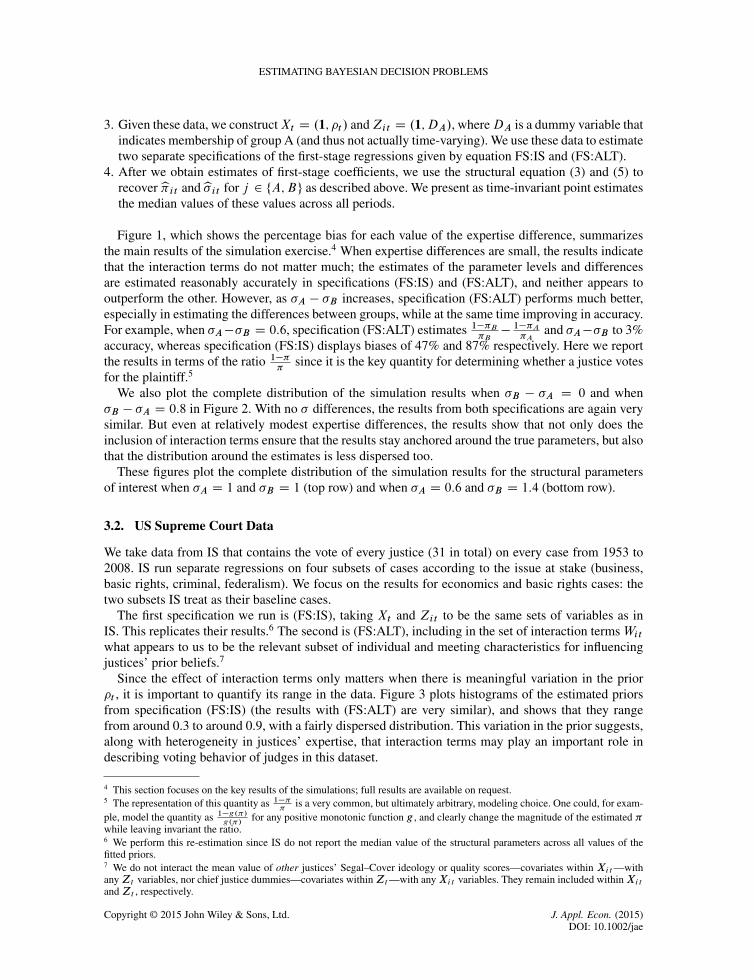
3. Given these data, we constructXt D .1; �t / andZit D .1;DA/, whereDA is a dummy variable thatindicates membership of group A (and thus not actually time-varying). We use these data to estimatetwo separate specifications of the first-stage regressions given by equation FS:IS and (FS:ALT).

4. After we obtain estimates of first-stage coefficients, we use the structural equation (3) and (5) torecoverb� it andb� it for j 2 ¹A;Bº as described above. We present as time-invariant point estimatesthe median values of these values across all periods.

Figure 1, which shows the percentage bias for each value of the expertise difference, summarizesthe main results of the simulation exercise.4 When expertise differences are small, the results indicatethat the interaction terms do not matter much; the estimates of the parameter levels and differencesare estimated reasonably accurately in specifications (FS:IS) and (FS:ALT), and neither appears tooutperform the other. However, as �A � �B increases, specification (FS:ALT) performs much better,especially in estimating the differences between groups, while at the same time improving in accuracy.For example, when �A��B D 0:6, specification (FS:ALT) estimates 1��B

�B� 1��A

�Aand �A��B to 3%

accuracy, whereas specification (FS:IS) displays biases of 47% and 87% respectively. Here we reportthe results in terms of the ratio 1��

�since it is the key quantity for determining whether a justice votes

for the plaintiff.5

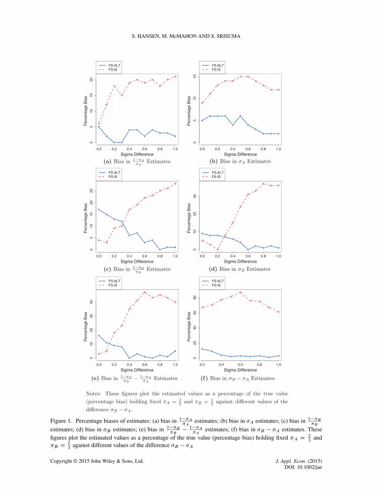
We also plot the complete distribution of the simulation results when �B � �A D 0 and when�B � �A D 0:8 in Figure 2. With no � differences, the results from both specifications are again verysimilar. But even at relatively modest expertise differences, the results show that not only does theinclusion of interaction terms ensure that the results stay anchored around the true parameters, but alsothat the distribution around the estimates is less dispersed too.

These figures plot the complete distribution of the simulation results for the structural parametersof interest when �A D 1 and �B D 1 (top row) and when �A D 0:6 and �B D 1:4 (bottom row).

3.2. US Supreme Court Data

We take data from IS that contains the vote of every justice (31 in total) on every case from 1953 to2008. IS run separate regressions on four subsets of cases according to the issue at stake (business,basic rights, criminal, federalism). We focus on the results for economics and basic rights cases: thetwo subsets IS treat as their baseline cases.

The first specification we run is (FS:IS), taking Xt and Zit to be the same sets of variables as inIS. This replicates their results.6 The second is (FS:ALT), including in the set of interaction terms Witwhat appears to us to be the relevant subset of individual and meeting characteristics for influencingjustices’ prior beliefs.7

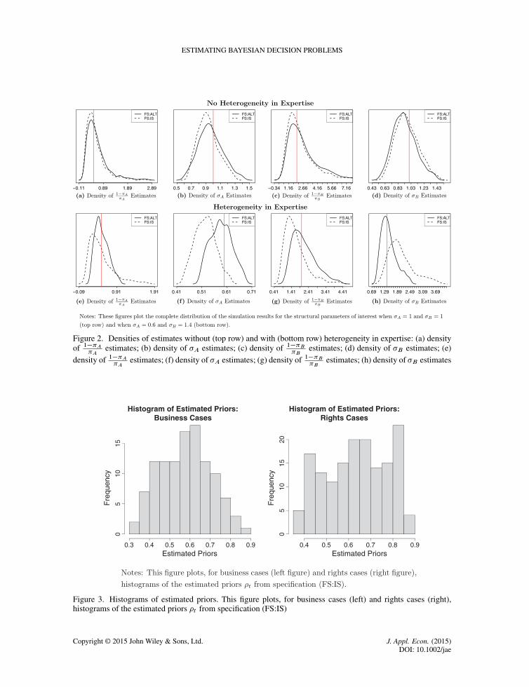
Since the effect of interaction terms only matters when there is meaningful variation in the prior�t , it is important to quantify its range in the data. Figure 3 plots histograms of the estimated priorsfrom specification (FS:IS) (the results with (FS:ALT) are very similar), and shows that they rangefrom around 0.3 to around 0.9, with a fairly dispersed distribution. This variation in the prior suggests,along with heterogeneity in justices’ expertise, that interaction terms may play an important role indescribing voting behavior of judges in this dataset.

4 This section focuses on the key results of the simulations; full results are available on request.5 The representation of this quantity as 1��

�is a very common, but ultimately arbitrary, modeling choice. One could, for exam-

ple, model the quantity as 1�g.�/g.�/

for any positive monotonic function g , and clearly change the magnitude of the estimated �while leaving invariant the ratio.6 We perform this re-estimation since IS do not report the median value of the structural parameters across all values of thefitted priors.7 We do not interact the mean value of other justices’ Segal–Cover ideology or quality scores—covariates within Xit—withanyZt variables, nor chief justice dummies—covariates withinZt—with anyXit variables. They remain included withinXitandZt , respectively.



0.0 0.2 0.4 0.6 0.8 1.0

05

1015

20

Sigma Difference

Per

cent

age

Bia

s

FS:ALTFS:IS

0.0 0.2 0.4 0.6 0.8 1.0

05

1015

Sigma Difference

Per

cent

age

Bia

s

FS:ALTFS:IS

0.0 0.2 0.4 0.6 0.8 1.0

05

1015

2025

Sigma Difference

Per

cent

age

Bia

s

FS:ALTFS:IS

0.0 0.2 0.4 0.6 0.8 1.0

010

2030

Sigma Difference

Per

cent

age

Bia

s

FS:ALTFS:IS

0.0 0.2 0.4 0.6 0.8 1.0

010

2030

40

Sigma Difference

Per

cent

age

Bia

s

FS:ALTFS:IS

0.2 0.4 0.6 0.8 1.0

020

4060

80

Sigma Difference

Per

cent

age

Bia

s

FS:ALTFS:IS

Figure 1. Percentage biases of estimates: (a) bias in 1��A�A

estimates; (b) bias in �A estimates; (c) bias in 1��B�B

estimates; (d) bias in �B estimates; (e) bias in 1��B�B

� 1��A�A

estimates; (f) bias in �B � �A estimates. Thesefigures plot the estimated values as a percentage of the true value (percentage bias) holding fixed �A D 2

3and

�B D13

against different values of the difference �B � �A



−0.11 0.89 1.89 2.89

FS:ALTFS:IS

0.5 0.7 0.9 1.1 1.3 1.5

FS:ALTFS:IS

−0.34 1.16 2.66 4.16 5.66 7.16

FS:ALTFS:IS

0.43 0.63 0.83 1.03 1.23 1.43

FS:ALTFS:IS

−0.09 0.91 1.91

FS:ALTFS:IS

0.41 0.51 0.61 0.71

FS:ALTFS:IS

0.41 1.41 2.41 3.41 4.41

FS:ALTFS:IS

0.69 1.29 1.89 2.49 3.09 3.69

FS:ALTFS:IS

Figure 2. Densities of estimates without (top row) and with (bottom row) heterogeneity in expertise: (a) densityof 1��A

�Aestimates; (b) density of �A estimates; (c) density of 1��B

�Bestimates; (d) density of �B estimates; (e)

density of 1��A�A

estimates; (f) density of �A estimates; (g) density of 1��B�B

estimates; (h) density of �B estimates

Histogram of Estimated Priors:Business Cases

Estimated Priors

Fre

quen

cy

0.3 0.4 0.5 0.6 0.7 0.8 0.9

05

1015

Histogram of Estimated Priors:Rights Cases

Estimated Priors

Fre

quen

cy

0.4 0.5 0.6 0.7 0.8 0.9

05

1015

20

Figure 3. Histograms of estimated priors. This figure plots, for business cases (left) and rights cases (right),histograms of the estimated priors �t from specification (FS:IS)



Table I. Re-estimation exercise

Business cases Rights cases

1��

estimates � estimates 1��

estimates � estimates

FS:IS FS:ALT FS:IS FS:ALT FS:IS FS:ALT FS:IS FS:ALT

Variance 0.123 0.068 0.011 0.006 0.451 0.056 0.037 0.006IQR 0.5249 0.3207 0.1532 0.1051 1.0802 0.3188 0.1925 0.0924Min. 0.294 0.333 0.396 0.392 0.275 0.290 0.360 0.415

Median 0.881 0.719 0.543 0.516 1.792 0.851 0.492 0.515Max. 1.567 1.431 0.759 0.699 2.509 1.240 1.255 0.726

Note: This table shows various measures of dispersion of the distribution across judges of the estimatedvalues of 1��

�and � when we specify equation FS:IS and (FS:ALT).

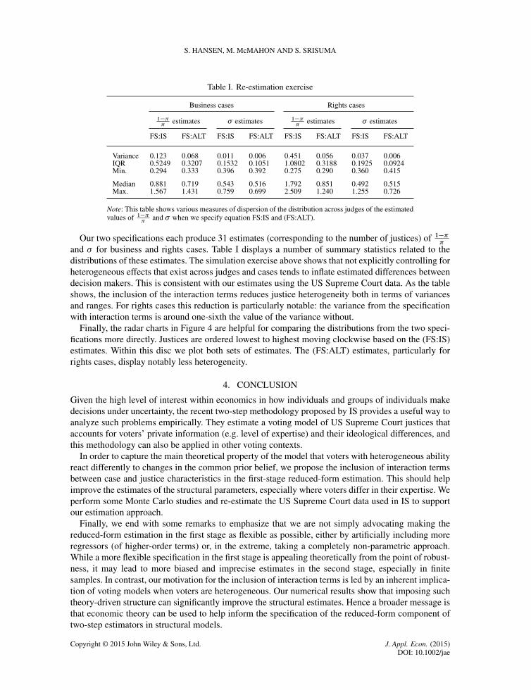
Our two specifications each produce 31 estimates (corresponding to the number of justices) of 1��

and � for business and rights cases. Table I displays a number of summary statistics related to thedistributions of these estimates. The simulation exercise above shows that not explicitly controlling forheterogeneous effects that exist across judges and cases tends to inflate estimated differences betweendecision makers. This is consistent with our estimates using the US Supreme Court data. As the tableshows, the inclusion of the interaction terms reduces justice heterogeneity both in terms of variancesand ranges. For rights cases this reduction is particularly notable: the variance from the specificationwith interaction terms is around one-sixth the value of the variance without.

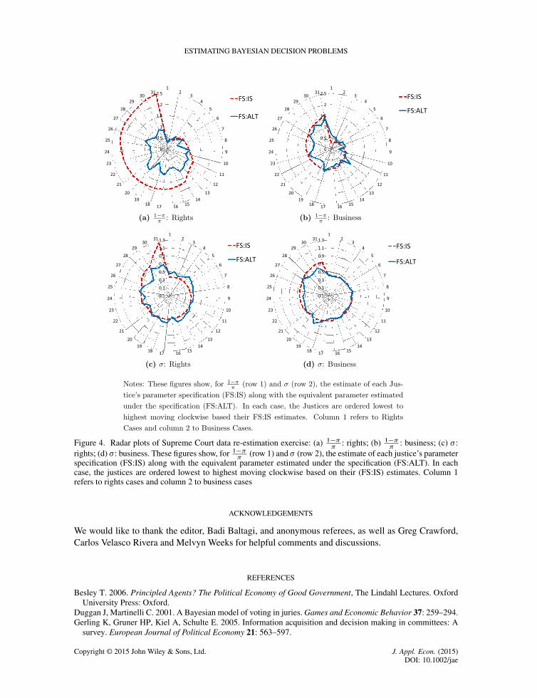
Finally, the radar charts in Figure 4 are helpful for comparing the distributions from the two speci-fications more directly. Justices are ordered lowest to highest moving clockwise based on the (FS:IS)estimates. Within this disc we plot both sets of estimates. The (FS:ALT) estimates, particularly forrights cases, display notably less heterogeneity.

4. CONCLUSION

Given the high level of interest within economics in how individuals and groups of individuals makedecisions under uncertainty, the recent two-step methodology proposed by IS provides a useful way toanalyze such problems empirically. They estimate a voting model of US Supreme Court justices thataccounts for voters’ private information (e.g. level of expertise) and their ideological differences, andthis methodology can also be applied in other voting contexts.

In order to capture the main theoretical property of the model that voters with heterogeneous abilityreact differently to changes in the common prior belief, we propose the inclusion of interaction termsbetween case and justice characteristics in the first-stage reduced-form estimation. This should helpimprove the estimates of the structural parameters, especially where voters differ in their expertise. Weperform some Monte Carlo studies and re-estimate the US Supreme Court data used in IS to supportour estimation approach.

Finally, we end with some remarks to emphasize that we are not simply advocating making thereduced-form estimation in the first stage as flexible as possible, either by artificially including moreregressors (of higher-order terms) or, in the extreme, taking a completely non-parametric approach.While a more flexible specification in the first stage is appealing theoretically from the point of robust-ness, it may lead to more biased and imprecise estimates in the second stage, especially in finitesamples. In contrast, our motivation for the inclusion of interaction terms is led by an inherent implica-tion of voting models when voters are heterogeneous. Our numerical results show that imposing suchtheory-driven structure can significantly improve the structural estimates. Hence a broader message isthat economic theory can be used to help inform the specification of the reduced-form component oftwo-step estimators in structural models.



Figure 4. Radar plots of Supreme Court data re-estimation exercise: (a) 1��

: rights; (b) 1��

: business; (c) � :rights; (d) � : business. These figures show, for 1��

�(row 1) and � (row 2), the estimate of each justice’s parameter

specification (FS:IS) along with the equivalent parameter estimated under the specification (FS:ALT). In eachcase, the justices are ordered lowest to highest moving clockwise based on their (FS:IS) estimates. Column 1refers to rights cases and column 2 to business cases

ACKNOWLEDGEMENTS

We would like to thank the editor, Badi Baltagi, and anonymous referees, as well as Greg Crawford,Carlos Velasco Rivera and Melvyn Weeks for helpful comments and discussions.

REFERENCES

Besley T. 2006. Principled Agents? The Political Economy of Good Government, The Lindahl Lectures. OxfordUniversity Press: Oxford.

Duggan J, Martinelli C. 2001. A Bayesian model of voting in juries. Games and Economic Behavior 37: 259–294.Gerling K, Gruner HP, Kiel A, Schulte E. 2005. Information acquisition and decision making in committees: A

survey. European Journal of Political Economy 21: 563–597.



Hansen S, McMahon M, Velasco Rivera C. 2014. Preferences or private assessments on a monetary policycommittee? Journal of Monetary Economics 67: 16–32.

Iaryczower M, Shum M. 2012. The value of information in the court: get it right, keep it tight. American EconomicReview 102: 202–237.

Iaryczower M, Lewis G, Shum M. 2013. To elect or to appoint? Bias, information, and responsiveness ofbureaucrats and politicians. Journal of Public Economics 97: 230–244.

Levy G. 2007. Decision making in committees: transparency, reputation, and voting rules. American EconomicReview 97: 150–168.

Maskin E, Tirole J. 2004. The politician and the judge: accountability in government. American Economic Review94: 1034–1054.

Prat A. 2005. The wrong kind of transparency. American Economic Review 95: 862–877.Sorensen P, Ottaviani M. 2000. Herd behavior and investment: Comment. American Economic Review 90:

695–704.


estimating bayesian decision problems with …

Documents