estimating information asymmetry in securities markets · estimating information asymmetry in...
TRANSCRIPT

Estimating Information Asymmetry in Securities Markets
Kerry Back
Jones Graduate School of Business and Department of Economics
Rice University, Houston, TX 77005, U.S.A.
Kevin Crotty
Jones Graduate School of Business
Rice University, Houston, TX 77005, U.S.A.
Tao Li
Department of Economics and FinanceCity University of Hong Kong, Kowloon, Hong Kong
Abstract
We propose and estimate a model of informed trading that is a hybrid of the PIN and
Kyle models. The relationships between price impacts and the estimated parameters
are consistent with the model’s theoretical predictions. We compare the hybrid model
estimates to PIN estimates. The probability of information events in the PIN model
is negatively correlated with the hybrid model’s estimated probability and with price
impacts. A composite information asymmetry measure explains more cross-sectional
variation in price impacts than does PIN, whose explanatory power stems primarily
from its liquidity trading parameter. The empirical results are consistent with the
model’s implication that both prices and order flows are necessary to identify private
information.
IVersions of this paper were presented under various titles at the University of Colorado, the SEC,the NYU Stern Microstructure Conference, and the University of Chicago Market Microstructureand High Frequency Data Conference. We thank Pete Kyle, Rob Engle, and seminar participantsfor helpful comments.
Email addresses: [email protected] (Kerry Back), [email protected] (KevinCrotty), [email protected] (Tao Li)
January 25, 2016

1. Introduction
Information asymmetry is a fundamental concept in economics, but its estimation
is challenging because private information is generally unobservable. A large literature
in finance and accounting utilizes the probability of informed trade (PIN) measure
of Easley, Kiefer, O’Hara, and Paperman (1996) to proxy for information asymmetry
because private information plays a key role in so many economic settings. However,
a number of papers argue that PIN does not measure information asymmetry.1
We propose a model of informed trading in securities markets that shares many
features of the PIN model of Easley et al. (1996) but in which informed trading is
endogenous as in Kyle (1985). We call this a hybrid PIN-Kyle model. We estimate
the model and compare the parameter estimates to PIN estimates. We calculate a
composite measure of information asymmetry, the expected average lambda (price
impact), based on the underlying hybrid model parameters. This measure incorpo-
rates both the probability and magnitude of information events as well as the amount
of liquidity trading.
The parameters of the hybrid model are estimated using both prices and order
flows. On the other hand, the PIN parameters depend only on order flows. The
hybrid model predicts that order flows alone cannot identify information asymmetry.
The intuition is quite simple. Consider, for example, a stock for which there is a large
amount of private information and another for which there is only a small amount of
private information. If it is anticipated that private information is more of a concern
for the first stock than for the second, then the first stock will be less liquid, other
things being equal. The lower liquidity will reduce the amount of informed trading,
possibly offsetting the increase in informed trading due to greater private information.
1We review the literature in Section 2.
1

In equilibrium, the amount of informed trading may be the same in both stocks,
despite the difference in information asymmetry. In general, the distribution of order
flows need not reflect the degree of information asymmetry when liquidity providers
react to information asymmetry and informed traders react to liquidity.
In the PIN model, order flows are, by assumption, independent of price changes.
This is the reason price changes are not used in estimating the parameters. In the
hybrid model, order flows depend on price changes, and both order flows and price
changes are useful for estimating the parameters. Thus, the reaction of liquidity
providers to information asymmetry and the reaction of informed traders to liquidity
are taken into account when estimating the hybrid model.
Theory predicts that stock orders have larger price impacts when information
events are more frequent or when information events are of larger magnitude. This is
true for both the hybrid and PIN models.2 We estimate the price impacts of orders
for a panel of stocks and regress price impacts on model parameters. Consistent with
theory, price impacts are higher for stocks that have more frequent information events,
larger magnitude events, or less volatile liquidity trading when these parameters are
estimated with the hybrid model. Contrary to theory, price impacts are lower for
stocks that have more frequent information events when the probability of information
events is estimated with the PIN model. In fact, the estimates of the probability of
an information event are negatively correlated across models.
Empirically, expected average lambda from the hybrid model explains a substan-
tial amount of cross-sectional variation in price impacts. However, we also find that
2There seems to be general agreement that at least a portion of the price impact of trades is dueto information asymmetry. Glosten and Harris (1988), Hasbrouck (1988), and Hasbrouck (1991)estimate models of trades and price changes in which both information asymmetry and inventorycontrol motives are accommodated, and all three papers conclude that information asymmetry isimportant.
2

PIN is positively related to price impacts cross-sectionally, despite the negative cor-
relation between the PIN probability of information events and price impacts. Eco-
nomically, this is primarily due to the fact that PIN reflects its model’s estimate of
the amount of liquidity trading. We run a horse race between the hybrid model’s ex-
pected average lambda and PIN by orthogonalizing PIN to expected average lambda.
The component of PIN collinear with expected average lambda explains five times the
variation in price impacts explained by the component of PIN orthogonal to expected
average lambda.
2. Literature
We first describe some of the microstructure literature that is related to our theo-
retical model. We then review the literature that uses PIN as a proxy for information
asymmetry as well as the literature critiquing the use of PIN as a measure of infor-
mation asymmetry or as a statistical model of the order flow distribution.
2.1. Microstructure Theory
We analyze a model that includes some features of the PIN model but in which
informed orders are endogenized as in Kyle (1985). Odders-White and Ready (2008)
analyze a Kyle model in which the probability of an information event is less than 1,
as it is in our model. However, Odders-White and Ready analyze a single-period
model, whereas we analyze a dynamic model. In a single-period model, because of
the net order having a mixture distribution, the conditional expectation of the asset
value given the net order is not a linear function of the net order. To make the model
tractable, Odders-White and Ready deviate from the usual Kyle model formulation
and do not require the asset price to equal its conditional expected value. Instead,
they only require that unconditional expected market maker profits are zero. They
find the pricing rule that is linear in the net order that has this “zero conditional
3

expected profits on average” property. Such a pricing rule would require commitment
by market makers, because it is not consistent with ex-post optimization by market
makers. In contrast, pricing in our model is consistent with ex-post optimization by
market makers: prices equal conditional expected values.
Related theoretical work includes Rossi and Tinn (2010), Banerjee and Green
(2015), Foster and Viswanathan (1995), and Chakraborty and Yilmaz (2004). Rossi
and Tinn solve a two-period Kyle model in which there are two large traders, one of
whom is certainly informed and one of whom may or may not be informed. In their
model, unlike ours, there are always information events. Banerjee and Green solve a
rational expectations model with myopic mean-variance investors in which investors
learn whether other investors are informed. They show that variation over time
in the perceived likelihood of informed trading induces volatility clustering. While
their model is quite different from ours, our model also exhibits volatility clustering.
Volatility follows the same pattern as Kyle’s lambda, which varies over time due to
variation in the market’s estimate of whether an information event occurred.
Foster and Viswanathan (1995) consider a series of single-period Kyle models in
which traders choose in each period whether to pay a fee to become informed. There
may be periods in which there are no informed traders. However, in their model,
it is always common knowledge how many traders choose to become informed, so,
in contrast to our model, there is no learning from orders about whether informed
traders are present.
Chakraborty and Yilmaz (2004) study a discrete-time Kyle model in which there
may or may not be an information event. Their main result is that the informed trader
will manipulate (sometimes buying when she has bad information and/or selling when
she has good information) if the horizon is sufficiently long. The primary difference
between their model and ours is that in their model the noise trade distribution has
4

finite support. If the low type trader never buys in their model, then an aggregate
order larger than the maximum of the noise trade distribution implies for certain that
the low type trader is not present. When the horizon is sufficiently long, it is optimal
for the low type trader to deviate from a strategy of never buying and to buy until the
aggregate order in a period is large enough that market makers put 100% probability
on her not being a low type. Then, she can begin selling. Consequently, it cannot
be an equilibrium in their model for low types to never buy and for high types to
never sell, when the horizon is sufficiently long. In contrast, market makers in our
model can never rule out any type of the informed trader until the end of the model,
so it does not strictly pay for a low type to pretend to be a high type or vice versa
(as we will show, and as is true in other continuous-time Kyle models, the informed
trader in our model is locally indifferent about buying or selling, so pretending to be
a different type is not suboptimal, but it does not occur in equilibrium).
A precursor to our paper is Li (2012), which solves a continuous-time Kyle model
in which the probability of an information event is less than 1 by applying filtering
theory to a transformation of the aggregate order process. The filtering solution
produces a stochastic differential equation for the equilibrium rather than a closed
form solution. The method of proof used in this paper shares some features with the
proof in Back and Crotty (2015).
2.2. PIN
A large literature in finance and accounting applies the PIN model to measure
information asymmetry. A portion of those papers assesses whether information risk
is priced. See, for example, Easley and O’Hara (2004), Duarte and Young (2009),
Mohanram and Rajgopal (2009), Easley, Hvidkjaer, and O’Hara (2002), Easley, Hvid-
kjaer, and O’Hara (2010), Akins, Ng, and Verdi (2012), Li, Wang, Wu, and He (2009),
and Hwang, Lee, Lim, and Park (2013). Many other papers use PIN as a proxy for
5

information asymmetry in a variety of applications ranging from corporate finance
(e.g., Chen, Goldstein, and Jiang, 2007; Ferreira and Laux, 2007) to accounting (e.g.,
Frankel and Li, 2004; Jayaraman, 2008).
Critiques of PIN can be classified into two groups. One set of papers argues that
it does not measure information asymmetry. The other set argues that its predictions
for the distributions of order flows are inconsistent with empirical distributions. The
first set of papers includes Aktas et al. (2007), Akay et al. (2012), and Duarte, Hu,
and Young (2014). Aktas et al. (2007) examine trading around merger announce-
ments. They show that PIN decreases prior to announcements. In contrast, percent-
age spreads and the permanent price impact of trades, measured as in Hasbrouck
(1991), rise before announcements, indicating the presence of information asymme-
try. They describe the decline in PIN prior to announcements as a PIN anomaly.
Akay et al. (2012) show that PIN is higher in the Treasury bill market than it is in
markets for individual stocks. Given that it is very doubtful that informed trading
in T-bills is a frequent occurrence, this is additional evidence that PIN is not mea-
suring information asymmetry. Duarte, Hu, and Young (2014) also examine merger
announcements. They estimate the parameters of the PIN model and then compute
the conditional probability of an information event each day. They show that the
conditional probability rises prior to merger announcements but stays elevated for up
to 30 days following announcements. They show that the high post-announcement
conditional probabilities are due to high turnover and argue that high turnover is
misidentified as private information by the PIN model.
Kim and Stoll (2014) analyze trading around earnings announcements and con-
sider subsamples based on the magnitude of the surprise in the announcement. They
find that order imbalances do not correlate with surprises and conclude that they
are not the result of informed trading. The evidence regarding order imbalances and
6

earnings surprises is additional evidence that measures based on order imbalances,
like PIN, cannot be measuring information asymmetry. However, the conclusion that
imbalances are not due to informed trading seems unwarranted. It is based on the
premise that informed order imbalances should be larger when surprises are larger,
which ignores equilibrium reactions. If there is a greater ex-ante likelihood of informed
trading in cases in which surprises are larger, then there will be less liquidity when
surprises are larger, other things being equal, so informed order imbalances should
not necessarily be larger when surprises are larger. Related evidence is provided by
Collin-Dufresne and Fos (2015), who document that both PIN and price impacts are
lower when activist investors accumulate positions in target firms ahead of required
regulatory 13-D filings. Collin-Dufresne and Fos (2012) show that the negative rela-
tionship between liquidity and informed trading is the equilibrium outcome in a Kyle
model due to informed traders reacting to changes in liquidity.
Venter and de Jongh (2006), Duarte and Young (2009), Gan, Wei, and Johnstone
(2014), and Duarte, Hu, and Young (2014) all show that the PIN model fails to fit
the empirical joint distribution of buy and sell orders. The first two papers propose
variations of the PIN model designed to provide a better fit to the data.
Easley, Lopez de Prado, and O’Hara (2012) propose a variation of PIN called
VPIN (Volume-synchronized PIN). They argue that signing individual transactions
as buys or sells in modern high-frequency markets may be problematic. Instead of
attempting to sign individual transactions, they assign a fraction of total volume
during a time interval to buys and the remaining fraction to sells based on the stan-
dardized price change during the time interval. They calculate VPIN using the order
imbalance implied by these estimates of buys and sells. Easley et al. (2011) claim
that VPIN predicted the “flash crash” of May 6, 2010. This claim and some other
claims regarding VPIN are challenged by Andersen and Bondarenko (2014b). See
7

also Easley et al. (2014) and Andersen and Bondarenko (2014a).
Easley, Engle, O’Hara, and Wu (2008) model daily buys and sells as being gener-
ated from the PIN model with time-varying parameters. The parameters are assumed
to be driven by buys and sells, much like the volatility in a GARCH model is an un-
observable variable that depends on returns and then determines the distribution
of future returns. When they estimate the model, they find that the informed and
uninformed arrival rates both increase with volume, whether orders are balanced or
unbalanced.
These variations on PIN are outside the scope of our paper. In comparing our
information asymmetry estimates to PIN, our focus is on the methodology used in
many papers in accounting and finance that use PIN as a proxy for information
asymmetry and estimate the parameters using daily buys and sells as in Easley et al.
(1996).
3. The Hybrid Model
The hybrid model includes two important features of PIN models—a probability
less than 1 of an information event and a binary asset value conditional on an infor-
mation event—and it also includes an optimizing (possibly) informed trader, as in the
Kyle (1985) model. Denote the time horizon for trading by [0, 1]. Assume there is a
single risk-neutral strategic trader. Assume this trader receives a signal S ∈ L,H
at time 0 with probability α, where L < 0 < H. Let pL and pH = 1 − pL denote
the probabilities of low and high signals, respectively, conditional on an information
event. With probability 1−α, there is no information event, and the trader also knows
when this happens. Let ξ denote an indicator for whether an information event has
occurred (ξ = 1 if yes and ξ = 0 if no). In addition to the private information, public
information can also arrive during the course of trading, represented by a martingale
8

V . Whether there was an information event, and, if so, whether the signal was low or
high becomes public information after the close of trading, producing an asset value
of V1 + ξS.
In addition to the strategic trades, there are liquidity trades represented by a
Brownian motion Z with zero drift and instantaneous standard deviation σ. Let Xt
denote the number of shares held by the strategic trader at date t (taking X0 = 0
without loss of generality), and set Yt = Xt+Zt. The processes Y and V are observed
by market makers. Denote the information of market makers at date t by FV,Yt .
One requirement for equilibrium in this model is that the price equal the expected
value of the asset conditional on the market makers’ information and given the trading
strategy of the strategic trader:
Pt = E[V1 + ξS | FV,Yt
]= Vt + E
[ξS | FV,Yt
]. (1)
We will show that there is an equilibrium in which Pt = Vt + p(t, Yt) for a function p.
This means that the expected value of ξS conditional on market makers’ information
depends only on cumulative orders Yt and not on the entire history of orders.
The other requirement for equilibrium is that the strategic trades are optimal.
Let θt denote the trading rate of the strategic trader (i.e., dXt = θt dt). The process
θ has to be adapted to the information possessed by the strategic trader, which is V ,
ξS, and the history of Z (in equilibrium, the price reveals Z to the informed trader).
The strategic trader chooses the rate to maximize
E
∫ 1
0
[V1 + ξS − Pt] θt dt = E
∫ 1
0
[ξS − p(t, Yt)] θt dt , (2)
with the function p being regarded by the informed trader as exogenous. In the
optimization, we assume that the strategic trader is constrained to satisfy the “no
doubling strategies” condition introduced in Back (1992), meaning that the strategy
9

must be such that
E
∫ 1
0
p(t, Yt)2 dt <∞
with probability 1.
Let N denote the standard normal distribution function, and let n denote the
standard normal density function. Set yL = σN−1(αpL) and yH = σN−1(1 − αpH).
This means that the probability mass in the lower tail (−∞, yL) of the distribution of
cumulative liquidity trades Z1 equals αpL, which is the unconditional probability of
bad news. Likewise, the probability mass in the upper tail (yH ,∞) of the distribution
of Z1 equals αpH , which is the unconditional probability of good news. Set
q(t, y, s) =
E[Z1 − Zt | Zt = y, Z1 < yL] if s = L ,
E[Z1 − Zt | Zt = y, yL ≤ Z1 ≤ yH ] if s = 0 ,
E[Z1 − Zt | Zt = y, Z1 > yH ] if s = H .
(3)
From the standard formula for the mean of a truncated normal, we obtain the fol-
lowing more explicit formula for q:
q(t, y, s)
σ√
1− t =
− n
(yL−yσ√1−t
)/N(yL−yσ√1−t
)if s = L ,[
n(yL−yσ√1−t
)− n
(yH−yσ√1−t
)]/[N(yH−yσ√1−t
)− N
(yL−yσ√1−t
)]if s = 0 ,
n(y−yHσ√1−t
)/N(y−yHσ√1−t
)if s = H .
(4)
The equilibrium described below can be shown to be the unique equilibrium in a
certain broad class, following Back (1992).
Theorem 1. There is an equilibrium in which the trading rate of the strategic trader
is
θt =q(t, Yt, ξS)
1− t . (5)
10

The equilibrium asset price is Pt = Vt + p(t, Yt), where the pricing function p is given
by
p(t, y) = L · N(yL − yσ√
1− t
)+H · N
(y − yHσ√
1− t
). (6)
In this equilibrium, the process Y is a martingale given market makers’ information
and has the same unconditional distribution as does the liquidity trade process Z; that
is, it is a Brownian motion with zero drift and standard deviation σ.
The last statement of the theorem implies that the distribution of order flows in
the model does not depend on the information asymmetry parameters α, H, and
L. Thus, if the model is correct, it is impossible to estimate those parameters using
order flows alone. In general, the theorem suggests that it may be difficult to identify
information asymmetry parameters using order flows alone, as discussed in the intro-
duction. When we estimate the hybrid model, we use both order flows and returns,
in contrast to the PIN model that only uses order flows.
Empirically, we test the relationship between α and price impacts of trades. Fig-
ure 1 plots the equilibrium price as a function of Yt for two different values of α. It
shows that the price is more sensitive to orders when α is larger. This is also true in
the PIN model. We test the relationship for both models. To investigate further how
the sensitivity of prices to orders depends on α in the hybrid model, we calculate the
price sensitivity—that is, we calculate Kyle’s lambda.
Theorem 2. In the equilibrium of Theorem 1, the asset price evolves as dPt =
dVt + λ(t, Yt) dYt, where Kyle’s lambda is
λ(t, y) = − L
σ√
1− t · n(yL − yσ√
1− t
)+
H
σ√
1− t · n(yH − yσ√
1− t
)(7)
Furthermore, Kyle’s lambda λ(t, Yt) is a martingale with respect to market makers’
11

information on the time interval [0, 1).
Kyle’s lambda is a stochastic process in our model, but we can easily relate the
expected average lambda to α. Because lambda is a martingale, the expected average
lambda is λ(0, 0). Substitute the definitions of yL and yH in (7) to compute3
λ(0, 0) = −Lσ
n(N−1(αpL)
)+H
σn(N−1(1− αpH)
). (8)
Figure 2 plots the expected average lambda as a function of α for two values of H,
taking L = −H. Doubling the signal magnitudes doubles lambda. Furthermore, the
expected average lambda is increasing in α.
4. Parameter Estimates
We estimate the hybrid model as well as the PIN model. We use trade and quote
data from TAQ for NYSE firms from 1993 through 2012.4 We sign trades as buys and
sells using the Lee and Ready (1991) algorithm: trades above (below) the prevailing
quote midpoint are considered buys (sells). If a trade occurs at the midpoint, then the
trade is classified as a buy (sell) if the trade price is greater (less) than the previous
differing transaction price.5 We use daily buys and sells to estimate the PIN model.
For the hybrid model, we sample prices and order imbalances hourly and at the close
and define order imbalances as shares bought less shares sold.
We estimate each of the models by maximum likelihood. For the PIN model, we
3If information events occur for sure (α = 1), then λ(0, 0) = (H − L) n(0)/σ. This is analogousto the result of Kyle (1985) that lambda is the ratio of the signal standard deviation to the standarddeviation of liquidity trading. Of course, it is not quite the same as Kyle’s formula, because we havea binary signal distribution, whereas the distribution is normal in Kyle (1985).
4We require that firms have intraday trading observations for at least 200 days within the year.We also require firms have the same ticker throughout the year and experience no stock splits.
5Prior to 2000, quotes are lagged five seconds when matched to trades. For 2000-2002, quotes arelagged one second. From 2003 on, quotes are matched to trades in the same second. To account forquote updates within a second, we use the interpolated time technique introduced by Holden andJacobsen (2014).
12

assume each day is a separate realization of the model, as is standard. We estimate
the models for each stock-year, assuming constant parameters within each year for
each stock, as is also standard. The likelihood function is provided in Appendix B,
as is the definition of PIN.
For the hybrid model, we also assume each day is a separate realization of the
model, and we estimate the model for each stock-year, assuming constant parameters
within each year for each stock. In each year for each stock, we assume there is
a parameter κ such that the possible signals on each trading day i of the year are
H = −L = κ. We assume that the possible signals are proportional to the observed
opening price on day i, Pi0, so κ is the magnitude of private information expressed as
a return. We also assume the public information process V is a geometric Brownian
motion on each day with a constant volatility δ. Appendix B derives the likelihood
function for the hybrid model under these assumptions. The likelihood function
depends on the signal magnitude κ, the probability α of information events, the
probability pL of a negative signal conditional on an information event, the standard
deviation σ of liquidity trading, and the volatility δ of public information.
4.1. Estimates of the Hybrid Model
Figure 3 displays the time-series of average estimates and the interquartile range
for the cross-section of stocks for the hybrid model. The average α is almost 70% in
the early part of the sample and falls to about 50% by the end of the sample, indi-
cating the likelihood of private information events, at least at the daily frequency we
study, has fallen on average. This effect starts in 2007 and is evident in the decrease
in the lower quartile of α estimates. The other components of private information
events are the magnitude κ of the signal and the likelihood pL of a bad event. Private
information κ initially rises during the late 1990s, but exhibits a strong downward
trend thereafter. The average pL indicates that the distribution of information is
13

relatively symmetric between positive and negative events. We combine these esti-
mates into a single composite measure of information asymmetry by calculating the
expected average lambda from Equation 8. The estimates indicate that the amount
of private information has fallen across the twenty year sample with the exception of
the late 1990s and the financial crisis.
In general, the standard deviation σ of order imbalances and the volatility δ of
public information appear to be roughly stationary. Despite the well-documented rise
of high-frequency trading and the associated sharp increase in trading volume, the
estimated volatility of order imbalances has remained fairly stable over the twenty
year sample. Public information volatility also spiked during the financial crisis. This
suggests private information is generally proportional to public information rather
than a fixed amount.
4.2. Testing Whether There is Always an Information Event in the Hybrid Model
Our hybrid model relaxes the assumption in Kyle (1985) of an information event
each period. A natural question is whether this relaxation is supported in the data.
The Kyle framework is nested in our model by the restriction that α = 1. Accordingly,
we estimate the model with this restriction. The standard likelihood ratio test of the
null that α = 1 against the alternative that α ∈ [0, 1] is rejected for 75% of the
firm-years (with a test size of 10%). However, the usual regularity conditions for
the likelihood ratio test require that the restriction not be at the boundary of the
parameter space. To address this issue, we bootstrap the distribution of the likelihood
ratio statistic for a random sample of 100 firm-years as in Duarte and Young (2009).
Specifically, for a given firm-year, we estimate the restricted model (α = 1) and
then simulate 500 firm-years under the null using the estimated (restricted) param-
eters. We then estimate the restricted and unrestricted models for each simulated
firm-year to obtain the distribution of the likelihood ratio under the null. The 90th
14

percentile of this distribution is the critical value to evaluate the empirical likelihood
ratio. These bootstrapped likelihood ratio tests reject the restricted Kyle model in fa-
vor of the hybrid model for 76 of the 100 randomly selected firm-years. The data thus
supports the conclusion that the probability of an information event is less than 1.
4.3. Estimates of the PIN Model
Figure 4 displays the time series of average parameter estimates for the PIN model.
The average estimated α is much lower than in the hybrid model at 30 to 40%. The
uninformed trading intensity ε and informed trading intensity µ each rise markedly in
the mid-2000’s reflecting the dramatic rise in trading volume. The average estimated
PIN falls from about 15% in 1993 to 10% in 2012.
4.4. Comparing the Models
Table 1 reports correlations of the hybrid model parameters with those of the
PIN model. The estimates of α for the hybrid model are negatively correlated with
the PIN estimates of α. The hybrid model α estimates are negatively correlated
with the noise trading parameters across both models (σ, ε), and are also negatively
correlated with the intensity of informed trading, µ, in the PIN model. The hybrid
α is positively correlated with PIN through its positive correlation with the ratio of
informed to uninformed trading (µε).
The composite measures of information asymmetry for the models are expected
average lambda and PIN. These measures are positively correlated (35%). This is
surprising given the lack of positive correlations of the α measures.
A potential explanation lies in the modeling of noise trading. Equation 8 shows
that expected average lambda is inversely related to the volatility of noise trading.
The PIN measure is also inversely related to noise trading (Equation B.5). Empiri-
cally, the hybrid model order imbalance volatility, σ, is positively correlated with the
15

PIN noise trading intensity, ε, as expected but is also positively correlated with both
the intensity of informed trading, µ, and the probability of an information event esti-
mated by the PIN model.6 One potential explanation for this that the unconditional
variance of order imbalances in the PIN model is:
2ε+ αµ(1 + µ)− (αµ(1− 2pL))2
which is generally increasing in both α and µ for the values estimated. Since PIN is
increasing in µε, the positive correlations of both the informed and uninformed trading
intensities with σ imply the relationship between PIN and σ is unclear. Empirically,
PIN and σ are negatively correlated since µε
and σ are negatively correlated. This
negative correlation explains why PIN and expected average lambda are positively
correlated despite very different estimates of the probability of an information event.
It is also interesting to see how estimates of private information differ in the cross-
section of firms across models. Table 2 reports average values of the parameters
within market capitalization deciles. For the hybrid model, the probability α of
an information event, the magnitude κ of information events, and expected average
lambda are all larger for smaller firms. Thus, the hybrid model estimates indicate
there is more private information for smaller firms. There is also more variation in
the public valuation of smaller firms, as shown in the δ estimates.
In contrast, the estimates of the PIN model show smaller probabilities of infor-
mation events for smaller firms. However, PIN is larger for smaller firms as a result
of large increases in noise trading intensity ε estimates as size increases. While the
informed trading intensity µ also increases with size, the noise trading component
dominates, leading to a declining ratio of informed to uninformed trading intensities
6µ and ε themselves are very highly correlated.
16

as a function of size. This effect dominates the modest increases in α as a function
of size, so PIN is lower as a result of increased noise trading identified by the PIN
model.
5. Predicting Price Impacts
In theory, price impacts should be larger when information asymmetry is higher,
for instance, when the probability α of information events is larger. This is true for
both the hybrid and the PIN model. It is shown in Section 3 for the hybrid model. For
the PIN model, the opening quoted spread is the product of PIN and the magnitude
of the information, H − L.7 Note that PIN is increasing in α and µ, and decreasing
in ε. In this section, we assess how cross-sectional variation in price impacts relates
to the estimated structural parameters from each model and functions of parameters
theoretically related to spreads in each model.
The percent price impact of a given trade k is calculated as:
Percent Price Impactk =2Dk(Pk+5 − Pk)
Pk, (9)
where Pk is the prevailing quote midpoint for trade k, Pk+5 is the quote midpoint five
minutes after trade k, and Dk equals 1 if trade k is a buy and −1 if trade k is a sell.
Goyenko, Holden, and Trzcinka (2009) use this measure as one of their high-frequency
liquidity benchmarks in a study assessing the quality of various liquidity measures
based on daily data.8 For a given stock-day, the estimate of the percent price impact
is the equal-weighted average price impact over all trades on that day. We average
these daily price impact estimates for each stock-year.
7See Equation 11 of Easley et al. (1996), which assumes pL = pH .8Holden and Jacobsen (2014) show that liquidity measures such as the percent price impact can
be biased when constructed from monthly TAQ data, so we follow their suggested technique inprocessing the data.
17

Figure 5 plots the time-series of the cross-sectional average and interquartile range
of the estimated price impacts. Over the twenty year sample, price impacts initially
rose over the 1990s before falling dramatically following the turn of the century, with
the brief exception of the financial crisis. Note that the time-series of the hybrid
model expected average lambda and the magnitude of private information, κ, exhibit
similar patterns (Figure 3).
Table 3 reports univariate Fama and MacBeth (1973) cross-sectional regressions of
price impacts on structural parameters in the hybrid and PIN models. Before running
the regressions, the structural parameters are winsorized at 1/99% and standardized
to have unit standard deviation. Price impacts are positively related to each of the
hybrid model parameters that measure private information (the probability α of an
information event and the magnitude κ of information events), and price impacts are
negatively related to the volatility of noise trading, σ. The expected average lambda
implied by the estimates explains over 30% of the cross-sectional variation in price
impacts and is strongly positively related to empirical price impacts.
Price impacts are higher for stocks with lower PIN α estimates. This is incon-
sistent with PIN α measuring the probability of private information events. Price
impacts are also negatively correlated with the estimated trading intensities µ and ε.
Theory predicts µ to be positively correlated with price impacts and ε to be nega-
tively correlated. PIN is increasing in the ratio of these intensities, µε, which correlates
positively with price impacts as predicted by theory. Table 1 indicates that µε
is neg-
atively correlated with both ε and µ as well as with σ from the hybrid model. Thus,
PIN estimates capture the inverse relationship between noise trading and spreads.
As a result, price impacts increase with PIN cross-sectionally in spite of the negative
relationship between α and price impacts.
Table 4 reports multivariate cross-sectional regressions controlling for a firm’s size
18

and price using the logarithm of market capitalization and the inverse stock price as
of the beginning of the year. Both size and price are strongly related to price im-
pacts (Breen, Hodrick, and Korajczyk, 2002); on average, these two control variables
explain 65% of the cross-sectional variation in price impact. Both expected average
lambda from the hybrid model and PIN remain significantly positively correlated with
price impacts, but the inclusion of size and price controls cuts the economic signifi-
cance of both information asymmetry measures. A one standard deviation change in
expected average lambda is associated with 2.25 basis point increase in price impact;
the univariate association was about twice as large. The reduction is much more dra-
matic for PIN. A one standard deviation in PIN is associated with less than a basis
point increase in price impacts. The magnitude of univariate relationship is almost 6
times the size of the multivariate relationship.
As discussed previously, expected average lambda from the hybrid model is posi-
tively correlated with PIN. How much of the variation in price impacts explained by
these measures captures common information? To determine this, we orthogonalize
PIN to expected average lambda via regression. This decomposition consists of the
portion of PIN collinear with expected average lambda (denoted PIN‖λ) and the
orthogonalized portion (denoted PIN ⊥ λ). Each component is scaled to have unit
standard deviation. Column (4) of Table 4 shows the relationship between price im-
pact and the decomposed PIN. The portion of PIN collinear with expected average
lambda is strongly positively related to the cross-section of price impacts. The com-
mon component across measures explains about five times more variation in price
impacts than the orthogonal component.
The theory in Section 3 shows that price impacts should be related to the inverse
of the standard deviation of liquidity trading. Accordingly, we orthogonalize PIN to
this measure and regress price impacts on the portion of PIN explained and unex-
19

plained by the inverse of noise trading along with the expected average lambda (last
column of Table 4). Each component is standardized to have unit standard deviation.
Expected average lambda again explains more of the cross-section of price impacts.
The coefficient on lambda is about four times as large as that on the portion of PIN
orthogonal to noise trading.
6. Further Comparison of the Models
In this section, we explain how the hypotheses of our model relate to those of
the PIN model. This facilitates the explanation in the next subsection of why the
endogeneity of informed orders in our model prevents the information asymmetry
parameters from being identified from order flows alone.
In the PIN model, there is a probability α of an information event. If there
is bad news, then informed sell orders arrive to the market as a Poisson process
with parameter µ. If there is good news, then informed buy orders arrive to the
market as a Poisson process with parameter µ. Regardless of whether there is an
information event, uninformed buy orders and uninformed sell orders each arrive as
Poisson processes with parameter ε. All of the Poisson processes are independent.
Throughout the time period of the model, market makers revise their beliefs about
whether an information event occurred and about the nature of any information event
based on the order flows. These revisions are in accordance with Bayes’ rule. For
example, if there has been a relatively large number of buy orders, then market makers
believe it likely that there has been good news. Market makers also revise their bid
and ask prices throughout the time period of the model as their beliefs change. These
are simple calculations presented in Equations (4) and (5) of Easley et al. (1996).
An important feature of the PIN model, which makes it easy to estimate but
which seems quite unrealistic, is that the informed order flow does not respond to
20

price changes. For example, when there is good news, informed buy orders continue
to arrive as a Poisson process with parameter µ throughout the model, regardless of
the price changes that have occurred previously. This is in part a consequence of the
binary signal assumption: the bid and ask are always strictly between the bad news
value and the good news value, so the asset is always somewhat overpriced when
there is bad news and somewhat underpriced when there is good news. However,
as illustrated in Figure 6, when informed orders are endogenized, the arrival rate
of informed orders depends on prior price changes even with a binary signal. When
prices have moved in the direction of the news, informed orders slow down, and, when
prices have moved in the opposite direction, informed orders speed up.
A second key feature of the PIN methodology is that, while prices can easily be
computed, they are not used to estimate the parameters of the model. The likelihood
function that is maximized is the density function of the sample of daily buys and
sells.
The primary differences between the hypotheses of the PIN model and the hy-
potheses of our model are:
• In the PIN model, informed trades and liquidity trades are independently dis-
tributed, conditional on an information event. However, in our model, the
informed trader reacts to past liquidity trades—for example, by buying less of
an undervalued asset when liquidity traders happen to erode the mispricing
through net purchases of the asset.
• In the PIN model, the distribution of informed trades conditional on an infor-
mation event is independent of the probability of an information event (they
are governed by separate parameters). In our model, if the probability of an in-
formation event is larger, then Kyle’s lambda is larger, and the informed trader
21

reacts to the decrease in liquidity by trading less.
• In the PIN model, liquidity-motivated buys and sells are independent Poisson
processes. In our model, net liquidity trades are a Brownian motion.
• In the PIN model, when there is no information event, all of the trades are
liquidity trades. In our model, when there is no information event, there is a
trader who recognizes that fact and who trades as a contrarian, selling when
liquidity traders buy and drive the price up and buying when they sell.
The changes to the PIN model described in the first two bullet points seem very
reasonable. Informed traders should trade less if liquidity traders happen to erode
the mispricing and should trade more when the opposite happens. Furthermore, they
should trade less in illiquid markets and more in liquid markets.
The third bullet point seems to be a relatively unimportant difference between
the models. If Poisson buys and sells are small and arrive frequently, then net orders
(buys minus sells) will be approximately a Brownian motion.9 The chief difference
between the Brownian and Poisson models is that buys and sells are not separately
defined in the Brownian model (a Brownian motion has infinite total variation, so it
is not the difference of two increasing processes). However, recent variations of PIN
(see the discussion of VPIN in Section 2) use only order imbalances—rather than
separate counts of buys and sells—to attempt to measure information asymmetry.
Our negative result on identification is directly applicable to those versions of PIN.
More generally, if information asymmetry cannot be identified from order imbalances,
as is true in our model, then it seems likely that it could not be identified from separate
counts of buys and sells either.
9Back and Baruch (2004) show that the equilibrium of a Kyle (1985) model with Brownian orderscan be approximated by a Glosten and Milgrom (1985) model with Poisson orders.
22

The change described in the fourth bullet point may be more controversial. The
existence of contrarian traders as described in the fourth bullet point seems likely
if there are always some traders who are best informed—corporate managers, for
example. This would be the case if information is truly idiosyncratic to the firm. If, on
the other hand, there is an industry or other aggregate component to the information,
then it is possible that no one knows when no one else has information. In that case,
the contrarian trader we postulate would not exist. Thus, we do not claim that our
model is applicable in all circumstances. Nevertheless, it appears to be reasonable in
some circumstances, and the empirical analysis in Sections 4 and 5 suggest that the
hybrid model’s structural estimates do capture information asymmetry.
6.1. Identification using Order Flows Alone
The key implication of Theorem 1 for the identification of information asymme-
try from order flows is the fact that the aggregate order imbalance Y1 is normally
distributed with mean zero and variance equal to the variance of liquidity trades.
Applications of the PIN model typically assume each day is a separate instance of the
model and use daily buys and sells to estimate the model parameters. If our model
describes reality and each day is a separate instance of the model, then the sample of
daily order imbalances is a sample of i.i.d. normal random variables with mean zero
and variance equal to the variance of liquidity trades.10 The distribution of the sam-
ple is invariant with respect to the frequency and magnitude of information events,
so the sample of daily order imbalances cannot identify information asymmetry.
The fact that Y1 is normally distributed with mean zero and variance equal to
the variance of liquidity trades is a consequence of the martingale property of Y (a
10Of course, we cannot know if a single day is a separate instance of either model. Many (long-lived) instances of private information may entail informed trading over multiple days (e.g., activistinvestors in Collin-Dufresne and Fos (2015)).
23

continuous martingale with quadratic variation over each time interval equal to the
length of the interval is automatically a Brownian motion). The martingale property
of Y is equivalent to unpredictability of informed orders in our model. As mentioned
before, informed orders are predictable in the PIN model, because informed traders
do not react to price changes in the PIN model.
The negative result on identification also holds in a more general model in which
there is a predictable component of order flows. In that model,
Y1 =
∫ 1
0
µt dt+ Y ∗1 ,
where Y ∗ is the sum of informed orders and unpredictable liquidity trades, and where
µ is adapted to the price process and hence adapted to Y ∗. Because informed orders
are unpredictable, Y ∗ is a martingale; therefore, it is a Brownian motion with its vari-
ance determined by the variance of liquidity trades. This implies that the distribution
of Y1 is again invariant with respect to the information asymmetry parameters.
Further insight into the identification issue can be gained by noting that, as in the
PIN model, the unconditional distribution of the order imbalance in our model is a
mixture of three conditional distributions. With probability αpL, Y1 is drawn from the
distribution conditional on a low signal; with probability αpH , Y1 is drawn from the
distribution conditional on a high signal; and with probability 1−α, Y1 is drawn from
the distribution conditional on no information event. The first two distributions have
nonzero means—there is an excess of sells over buys in the first and an excess of buys
over sells in the second. This is also analogous to the PIN model. Thus, one might
conjecture that changing α—thereby changing the likelihood of drawing from the
first two distributions—will alter the unconditional distribution of Y1. If so, then one
could perhaps identify α from the distribution of Y1. In the PIN model, it is indeed
true that changing α, holding other parameters constant, alters the unconditional
24

distribution of the order imbalance. However, it is not true in our model, because
the distribution of informed trades in our model depends endogenously on α due to
liquidity depending on α. With a larger alpha, the market is less liquid (see Section 3)
and the informed trader trades less aggressively. Thus, the distributions over which we
are mixing change when the mixture probabilities change, leaving the unconditional
distribution of Y1 invariant with respect to α.
The change in the conditional distributions is illustrated in Figure 7. The top and
bottom panels of Figure 7 show that the strategic trader trades more aggressively
when an information event occurs if an information event is less likely (α = 0.1 versus
α = 0.5). This equilibrium reaction of informed trading to exogenous changes in the
probability of information events is missing in the PIN model, in which informed
trading is exogenously determined. It is a key feature of our model that results in
the probability of information events being unidentified by the distribution of order
imbalances. The unconditional distribution of Y1 is standard normal for both α = 0.1
and α = 0.5 in Figure 7, so we cannot hope to use the unconditional distribution to
recover α.
Continuing with the example in Figure 7, calculate the expected absolute order
imbalance as
αpLE[|Y1| | ξ = 1, S = L
]+ (1− α)E
[|Y1| | ξ = 0
]+ αpHE
[|Y1| | ξ = 1, S = H
],
with σ = 1 and pL = pH = 1/2. If α = 0.5, then the expected absolute order
imbalance is
1
4× 1.27 +
1
2× 0.32 +
1
4× 1.27 = 0.80 .
On the other hand, if α = 0.1, then the expected absolute order imbalance is
1
20× 2.06 +
9
10× 0.66 +
1
20× 2.06 = 0.80 .
25

Again, we see that informed trading is more aggressive when information events occur
if such events are less likely. Here, it is clear that the endogenous change in informed
trading exactly offsets the exogenous change in the likelihood of information events.
In other words, the endogenous changes in the distributions over which we are mixing
exactly offset the changes in the mixing probabilities (this is true even with pL 6= pH).
On the other hand, under the assumptions of the PIN model, the expected absolute
order imbalance varies with α (see Easley et al., 2008, p. 176, for a discussion of how
the absolute order imbalance is related to α and to PIN under the assumptions of the
PIN model).
The previous paragraphs describe the invariance of the unconditional distribution
of Y1 with respect to α. The other important parameters governing information
asymmetry are L and H. For example, if the possible signals L and H are both small
in absolute value, then information asymmetry is a minor concern even if information
events occur frequently. Order flows cannot identify L and H in our model. In fact,
L and H do not affect even the conditional distributions shown in Figure 7; thus,
they do not affect the unconditional distribution of Y1.
Of course, identifying the information asymmetry parameters from the distribu-
tion of order imbalances is a very different issue from using order imbalances to update
the probability of an information event in a particular instance of the model. Condi-
tional on knowledge of the parameters, the order imbalance does help in estimating
whether an information event occurred in a particular instance of the model; in fact,
the market makers in the model update their beliefs regarding the occurrence of an
information event based on the order imbalance. So, we can compute
prob(info event | Yt, parameters) ,
and this probability does depend on the information asymmetry parameters. We
26

could use this to identify the information asymmetry parameters if we had data on
order imbalances and data on whether information events occurred. Of course, we do
not have data of the latter type. Theorem 1 shows that the likelihood function of the
information asymmetry parameters given only data on order imbalances is a constant
function of those parameters; hence, the order imbalances alone cannot identify them.
6.2. Empirical and Model-Implied Unconditional Order Flow Distributions
The hybrid and PIN models have different implications for the unconditional dis-
tribution of order imbalances. For both models, the order flow distribution is a mix-
ture distribution (i.e., of the good, bad, no event distributions), but Figure 8 shows
how the distributions can differ based on the underlying parameter values. Under the
hybrid model, end-of-day order flows are normally distributed with standard devia-
tion σ. However, in the PIN model, order imbalances can be trimodal. Indeed, this
is generally the case for order imbalances implied by structural estimates of the PIN
model. The bottom row of Figure 8 plots the model-implied order imbalance distribu-
tion for the smallest and largest NYSE firm deciles under PIN. The PIN model must
fit volume as well as order imbalances since the input data are buy and sell volumes.
On the other hand, the hybrid model need only fit the order flow distribution.
How do the model-implied order imbalance distributions compare to those found
empirically? Figure 9 shows the empirical standardized order imbalance distributions
for the smallest and largest NYSE size deciles in our sample. The figure displays both
share and trade imbalances since these are the underlying data for the hybrid and PIN
models, respectively. The empirical distributions do not exhibit strong multimodal
behavior. This is more consistent with the modeling assumption of the hybrid model
than that of the PIN model.
27

7. Conclusion
We propose a model of informed trading that is a hybrid of the PIN and Kyle
models. Information events occur with probability less than one as in the PIN model
(but unlike the Kyle model). However, unlike the PIN model, informed orders are
endogenously determined as in the Kyle model. We estimate the model and compare
the parameter estimates to PIN estimates. The relationships between price impacts
and the estimated hybrid model parameters are consistent with the theoretical pre-
dictions of the model. This is not true for the PIN parameters. The probability
of information events in the PIN model is negatively correlated with price impacts
and negatively correlated with the probability of information events estimated from
the hybrid model. A composite measure of the hybrid model information asymme-
try parameters explains much more cross-sectional variation in price impacts than
does PIN. We also show that the explanatory power of PIN for price impacts is due
primarily to the liquidity trading parameter. The improved empirical performance
likely results from the use of both price and order flow data in estimation. Indeed,
the model implies that both prices and order flows are needed to identify private
information.
28

Appendix A. Proofs
The process Y described in the following lemma is a variation of a Brownian bridge.
It differs from a Brownian bridge in that the endpoint is not uniquely determined but
instead is determined only to lie in an interval—either the lower tail (−∞, yL), the
upper tail (yH ,∞) or the middle region [yL, yH ]—depending on whether there is an
information event and whether the news is good or bad. Part (C) of the lemma follows
immediately from the preceding parts, because the probability (A.3) is the probability
that Y1 /∈ [yL, yH ] calculated on the basis that Y is an FY –Brownian motion with zero
drift and standard deviation σ.
Lemma. Let N denote the standard normal distribution function. Let FY = FYt |
0 ≤ t ≤ 1 denote the filtration generated by the stochastic process Y defined by
Y0 = 0 and
dYt =q(t, Yt, ξS)
1− t dt+ dZt . (A.1)
Then, the following are true:
(A) Y is an FY –Brownian motion with zero drift and standard deviation σ.
(B) With probability one,
ξ = 1 and S = L ⇒ Y1 < yL , (A.2a)
ξ = 0 ⇒ yL ≤ Y1 ≤ yH , (A.2b)
ξ = 1 and S = H ⇒ Y1 > yH . (A.2c)
(C) For each t < 1, the probability that ξ = 1 conditional on FYt is
N
(yL − Ytσ√
1− t
)+ 1− N
(yH − Ytσ√
1− t
). (A.3)
29

Proof of the Lemma. Set
k(1, y, s) =
1y<yL if s = L ,
1yL≤y≤yH dz if s = 0 ,
1y>yH if s = H ,
and, for t < 1,
k(t, y, s) =
N(yL−yσ√1−t
)dz if s = L ,
N(yH−yσ√1−t
)− N
(yL−yσ√1−t
)dz if s = 0 ,
N(y−yHσ√1−t
)if s = H .
Define
`(t, y, s) =∂ log k(t, y, s)
∂y,
for t < 1. Then, (1− t)σ2`(t, y, s) = q(t, y, s) for t < 1, and the stochastic differential
equation (A.1) can be written as
dYt = σ2 `(t, Yt, ξS) dt+ dZt (A.4)
The process Y is an example of a Doob h-transform—see Rogers and Williams (2000).
To put (A.4) in a more standard form, define the two-dimensional process Yt =
(ξS, Yt) with random initial condition Y0 = (ξS, 0), and augment (A.4) with the
equation d(ξS) = 0. The existence of a unique strong solution Y to this enlarged
system follows from Lipschitz and growth conditions satisfied by `. See Karatzas and
Shreve (1988, Theorem 5.2.9).
The uniqueness in distribution of weak solutions of stochastic differential equations
30

(Karatzas and Shreve, 1988, Theorem 5.3.10) implies that we can demonstrate Prop-
erties (A) and (B) by exhibiting a weak solution for which they hold. To construct
such a weak solution, define a new measure Q on F1 using k(1, Z1, ξS)/k(0, 0, ξS)
as the Radon-Nikodym derivative. The definition of k implies that k(t, Zt, ξS) is the
Ft–conditional expectation of the indicator function k(1, Z1, ξS), so k(t, Zt, ξS) is a
martingale on the filtration F. By Girsanov’s Theorem, the process Z∗ defined by
Z∗0 = 0 and
dZ∗t = −σ2 `(t, Zt, ξS) dt+ dZt
is a Brownian motion (with zero drift and standard deviation σ) on the filtration F
relative to Q. It follows that Z is a weak solution of (A.4) relative to the Brownian
motion Z∗ on the filtered probability space (Ω,F,Q).
To establish Property (A) for the weak solution, we need to show that Z is a
Brownian motion on (Ω,G,Q). Because Z is a Brownian motion on (Ω,G,P), it
suffices to show that Q = P when both are restricted to G1. This holds if for all
t1 < · · · < tn ≤ 1 and all Borel B we have
P((Zt1 , . . . , Ztn) ∈ B) = Q((Zt1 , . . . , Ztn) ∈ B) . (A.5)
The right-hand side of (A.5) equals
E
[k(1, Z1, ξS)
k(0, 0, ξS)1B(Zt1 , . . . , Ztn)
],
31

which can be represented as the following sum:
αpLE
[k(1, Z1, ξS)
k(0, 0, ξS)1B(Zt1 , . . . , Ztn) | ξS = L
]+ (1− α)E
[k(1, Z1, ξS)
k(0, 0, ξS)1B(Zt1 , . . . , Ztn) | ξ = 0
]+ αpHE
[k(1, Z1, ξS)
k(0, 0, ξS)1B(Zt1 , . . . , Ztn) | ξS = H
].
Using the definitions of yL, yH , and k, this equals
E[1Z1<yL1B(Zt1 , . . . , Ztn) | ξS = L
]+ E
[1yL≤Z1≤yL1B(Zt1 , . . . , Ztn) | ξ = 0
]+ E
[1Z1>yH1B(Zt1 , . . . , Ztn) | ξS = H
].
The P–independence of Z and ξS imply that the conditional expectations equal the
unconditional expectations, so adding the three terms gives
E [1B(Zt1 , . . . , Ztn)] = P((Zt1 , . . . , Ztn) ∈ B) .
This completes the proof that Z is a Brownian motion on (Ω,G,Q).
To establish Property (B) for the weak solution of (A.4), we need to show that
Q(Z1 < yL | ξS = L) = 1 , (A.6a)
Q(yL ≤ Z1 ≤ yH | ξ = 0) = 1 , (A.6b)
Q(Z1 > yH) | ξS = H) = 1 . (A.6c)
32

Consider (A.6a). We have
Q(ξS = L) = E
[k(1, Z1, ξS)
k(0, 0, ξS)1ξS=L
]= E
[k(1, Z1, L)
k(0, 0, L)1ξS=L
]= E
[1Z1<yL1ξS=L
]/αpL
= αpL ,
using the definition of k for the third equality and the P–independence of Z and ξS
for the last equality. By similar reasoning,
Q(Z1 < yL, ξS = L) = E
[k(1, Z1, ξS)
k(0, 0, ξS)1Z1<yL1ξS=L
]= E
[k(1, Z1, L)
k(0, 0, L)1Z1<yL1ξS=L
]= E
[1Z1<yL1ξS=L
]/αpL
= αpL .
Thus,
Q(Z1 < yL | ξS = L) =Q(Z1 < yL, ξS = L)
Q(ξS = L)=αpLαpL
= 1 .
Conditions (A.6b) and (A.6c) can be verified by the same logic.
Proof of Theorem 1. It is explained in the text why the equilibrium condition (1)
holds. It remains to show that the strategy (5) is optimal for the informed trader.
Let G def= Gt | 0 ≤ t ≤ T denote the completion of the filtration generated by Z,
form the enlarged filtration with σ–fields Gt ∨ σ(ξS), and let F def= Ft | 0 ≤ t ≤ T
denote the completion of the enlarged filtration. The filtration F represents the
informed trader’s information.
33

Define
J(1, y, L) = −L(y − yL)1y>yL +H(y − yH)1y>yH ,
J(1, y, 0) = −L(yL − y)1y<yL +H(y − yH)1y>yH ,
J(1, y,H) = −L(yL − y)1y<yL +H(yH − y)1y<yH .
For t < 1 and s ∈ L, 0, H, set J(t, y, s) = E[J(t, Z1, s) | Zt = y]. Then, J(t, Zt, ξS)
is an F–martingale, so it has zero drift. From Ito’s formula, its drift is
∂
∂tJ(t, Zt, ξS) +
1
2σ2 ∂
2
∂z2J(t, Zt, ξS) .
Equating this to zero, Ito’s formula implies
J(1, Y1, ξS) = J(0, 0, ξS) +
∫ 1
0
dJ(t, Yt, ξS) = J(0, 0, ξS) +
∫ 1
0
∂J(t, Yt, ξS)
∂ydYt .
Therefore,
E[J(1, Y1, ξS)− J(0, 0, ξS)] = E
∫ 1
0
∂J(t, Yt, ξS)
∂ydYt . (A.7)
To calculate ∂J(t, y, s)/∂y, use the fact that, by independent increments,
J(t, y, s) = E[J(t, Z1, s) | Zt = y] = E[J(t, Z1 − Zt + y, s)]
to obtain
∂J(t, y, s)
∂y= E
[∂
∂yJ(t, Z1 − Zt + y, s)
].
34

Now, note that, for any real number a excluding the kinks at yL − y and yH − y,
∂
∂yJ(1, a+ y, L) = −L1a>yL−y +H1a>yH−y ,
∂
∂yJ(1, a+ y, 0) = L1a<yL−y +H1a>yH−y ,
∂
∂yJ(1, a+ y,H) = L1a<yL−y −H1a<yH−y .
Therefore,
∂J(t, y, L)
∂y= −LN
(y − yLσ√
1− t
)+H N
(y − yHσ√
1− t
),
∂J(t, y, 0)
∂y= LN
(yL − yσ√
1− t
)+H N
(y − yHσ√
1− t
),
∂J(t, y,H)
∂y= LN
(yL − yσ√
1− t
)−H N
(yH − yσ√
1− t
).
Now, the definition (6) gives us
∂J(t, y, s)
∂y= p(t, y)− s
for all s ∈ L, 0, H. Substituting this into (A.7) gives us
E[J(1, Y1, ξS)− J(0, 0, ξS)] = E
∫ 1
0
[p(t, Yt)− ξS] dYt . (A.8)
The “no doubling strategies” condition implies that∫p dZ is a martingale, so the
right-hand side of this equals
E
∫ 1
0
[p(t, Yt)− ξS]θt dt .
35

Rearranging produces
E
∫ 1
0
[ξS − p(t, Yt)]θt dt = E[J(0, 0, ξS)− J(1, Y1, ξS)] ≤ E[J(0, 0, ξS)] ,
using the fact that J(1, y, s) ≥ 0 for all (y, s) for the inequality. Thus, E[J(0, 0, ξS)]
is an upper bound on the expected profit, and the bound is achieved if and only if
J(1, Y1, ξS) = 0 with probability one. By the definition of J(1, y, s), this is equivalent
to Y1 < yL with probability one when ξS = L, yL ≤ Y1 ≤ yH with probability one
when ξ = 0, and Y1 > yH with probability one when ξS = H. By part (B) of the
proposition, the strategy (5) is therefore optimal.
Proof of Theorem 2. By Ito’s formula and the fact that (dY )2 = (dZ)2 = σ2 dt, we
have
dp(t, Yt) =
(pt(t, Yt) +
1
2σ2pyy(t, Yt)
)dt+ py(t, Yt) dYt ,
where we use subscripts to denote partial derivatives. Both Y and p(t, Yt) are mar-
tingales with respect to the market makers’ information, so the drift term must be
zero. That can also be verified by direct calculation of the partial derivatives, using
the formula (6) for p(t, y). Thus,
dp(t, Yt) = py(t, Yt) dYt .
A direct calculation based on the formula (6) for p(t, y) shows that py(t, y) = λ(t, y)
defined in (7).
To see that λ(t, Yt) is a martingale for t ∈ [0, 1), with respect to market makers’
36

information, we can calculate, for t < u < 1,
E[λ(u, Yu) | Yt = y] = − L
σ√
1− u ·∫ ∞−∞
n
(yL − y′σ√
1− u
)f(y′ | u− t, y)dy′
+H
σ√
1− u ·∫ ∞−∞
n
(yH − y′σ√
1− u
)f(y′ | u− t, y)dy′ ,
where f(· | τ, y) denotes the normal density function with mean y and variance σ2τ .
A straightforward calculation shows that this equals λ(t, y). For example, to evaluate
the first term, use the fact that
1
σ√
1− u n
(yL − y′σ√
1− u
)f(y′ | u− t, y)
=1
σ√
1− t n
(yL − yσ√
1− t
)× 1√
2πσ2(1− u)(u− t)/(1− t)
× exp
(−(
1− t2(1− u)(u− t)σ2
)(y′ − (1− u)y + (u− t)yL
1− t
)2),
which integrates to
1
σ√
1− t n
(yL − yσ√
1− t
),
because the other factors constitute a normal density function.
37

Appendix B. Likelihood Functions
Appendix B.1. Hybrid Model
Assume the trading period [0, 1] corresponds to a day. This implies that any
private information becomes public before trading opens on the following day.11 We
can estimate the model parameters using intraday price and order flow information. If
we assume further that the model parameters are stable over time, then the price and
order flow information from multiple days can be merged to estimate the parameters
with greater precision.
The opening price on each day i is Pi0def= E[Vi1 + ξiSi] = Vi0. To obtain
stationarity, we assume that the signal Si on day i is proportional to the observed
opening price Pi0. This construction causes the pricing function to be day-specific,
and we denote it by pi(t, y). In fact,
pi(t, y) = Pi0 × p(t, y)
where p(t, y) is defined in Theorem 1. We specify that H = −L = κ in the empirical
implementation. Under this specification, the pricing function expressed in returns is
given by:
p(t, Yt) =
−κ1(Yt < zL) + κ1(Yt > zH) if t = 1 ,
−κF (zL|t, Yt) + κ(1− F (zH |t, Yt)) if t < 1
where F (z|t, Yt) is the normal distribution function with mean Yt and variance (1 −
t)σ2.
11In contrast to Odders-White and Ready (2008), our estimation does not use overnight returns.In our theoretical model, private information that is made public after the close of trading is in-corporated into prices before trading ends (convergence to strong-form efficiency). Thus, overnightreturns in our model are due to arrival of new public information, which does not aid in estimatingthe model.
38

The price at time t on day i is Vit + pi(t, Yit), so the gross return through time t is
PitPi0
=VitVi0
+pi(t, Yit)
Pi0=VitVi0
+ p(t, Yit) . (B.1)
Assume
dVitVit
= δ dBit
for a constant δ and a Brownian motion Bi, so we have
PitPi0
= p(t, Yit) + eδBit−δ2t/2 .
Assume the price and order imbalance are observed at times t1, . . . , tk+1 each day
with tk+1 = 1 being the close and the other times being equally spaced: tj = j∆
for ∆ > 0 and j ≤ k. Let Pij denote the observed price and Yij the observed order
imbalance at time tj on date i. Define
Γ =
1
2
...
k
1/∆
, Σ =
1 1 · · · 1 1
1 2 · · · 2 2
......
......
...
1 2 · · · k k
1 2 · · · k 1/∆
.
On each day i, the vector Yi = (Yi,t1 , . . . , Yi,tk+1)′ is normally distributed with
mean 0 and covariance matrix σ2∆Σ. Set
Uij = log
(PijPi0− p(tj, Yij)
)(B.2)
and Ui = (Ui1, . . . , Ui,k+1)′. The density function of (Pi1/Pi0, . . . , Pi,k+1/Pi0) condi-
tional on Yi is
f(Ui1, . . . Ui,k+1)e−
∑k+1j=1 Uij ,
39

where f denotes the multivariate normal density function with mean vector−(δ2∆/2)Γ
and covariance matrix δ2∆Σ.
Let Li denote the log-likelihood function for day i. Dropping terms that do not
depend on the parameters, we have
− Li = (k + 1) log σ +1
2σ2∆Y ′i Σ
−1Yi + (k + 1) log δ
+1
2δ2∆
(Ui +
δ2∆
2Γ
)′Σ−1
(Ui +
δ2∆
2Γ
)+
k+1∑j=1
Uij .
Using the facts that Γ′Σ−1 = (0, . . . , 0, 1) and Γ′Σ−1Γ = 1/∆, this simplifies to
− Li = (k + 1) log σ +1
2σ2∆Y ′i Σ
−1Yi + (k + 1) log δ
+1
2δ2∆U ′iΣ
−1Ui +1
2Ui,k+1 +
δ2
8+
k+1∑j=1
Uij .
Hence, the log-likelihood function L for an observation period of n days satisfies
− L = n(k + 1) log σ +1
2σ2∆
n∑i=1
Y ′i Σ−1Yi + n(k + 1) log δ
+1
2δ2∆
n∑i=1
U ′iΣ−1Ui +
nδ2
8+
n∑i=1
(k∑i=1
Uik +3
2Ui,k+1
). (B.3)
We minimize (B.3) in α, κ, pL, σ, and δ (note that κ and pL enter L because they
affect the function p that enters L via (B.2)). We sample every hour and at the close,
so ∆ = 1/6.5.
Appendix B.2. PIN Model
The likelihood of the PIN model is:
L(B, S|α, pL, µ, ε) =T∏t=1
(1− α)
[exp (−2ε) εBt+St
Bt!St!
]+αpL
[exp (−(µ+ 2ε)) (µ+ε)StεBt
Bt!St!
]+α(1− pL)
[exp (−(µ+ 2ε)) (µ+ε)BtεSt
Bt!St!
] (B.4)
40

where Bt (St) is the number of buys (sells) on day t, α is the probability of an
information event, pL is the probability that an information event is bad news, and µ
and ε are the arrival rates of informed and uninformed traders. PIN, the probability
of informed trade, is given by the formula:
PIN =αµ
αµ+ 2ε. (B.5)
41
References
Akay, O., Cyree, K. B., Griffiths, M. D., Winters, D. B., 2012. What does PIN
identify? Evidence from the T-bill market. Journal of Financial Markets 15, 29–46.
Akins, B., Ng, J., Verdi, R. S., 2012. Investor competition over information and the
pricing of information asymmetry. The Accounting Review 87 (1), 35–58.
Aktas, N., de Bodt, E., Declerck, F., Van Oppens, H., 2007. The PIN anomaly around
M&A announcements. Journal of Financial Markets 10 (2), 160–191.
Andersen, T., Bondarenko, O., 2014a. Reflecting on the VPIN dispute. Journal of
Financial Markets 17, 53–64.
Andersen, T., Bondarenko, O., 2014b. VPIN and the flash crash. Journal of Financial
Markets 17, 1–46.
Back, K., 1992. Insider trading in continuous time. Review of Financial Studies 5,
387–409.
Back, K., Baruch, S., 2004. Information in securities markets: Kyle meets Glosten
and Milgrom. Econometrica 72, 433–465.
Back, K., Crotty, K., 2015. The informational role of stock and bond volume. Review
of Financial Studies 28, 1381–1427.
Banerjee, S., Green, B., 2015. Signal or noise? Uncertainty and learning about
whether other traders are informed. Journal of Financial Economics 117, 398–423.
Breen, W. J., Hodrick, L. S., Korajczyk, R. A., 2002. Predicting equity liquidity.
Management Science 48 (4), 470–483.
42

Chakraborty, A., Yilmaz, B., 2004. Manipulation in market order models. Journal of
Financial Markets 7, 187–206.
Chen, Q., Goldstein, I., Jiang, W., 2007. Price informativeness and investment sensi-
tivity to stock price. Review of Financial Studies 20 (3), 619–650.
Collin-Dufresne, P., Fos, V., 2012. Insider trading, stochastic liquidity and equilibrium
prices. Working paper, Boston College and EPFL.
Collin-Dufresne, P., Fos, V., 2015. Do prices reveal the presence of informed trading?
Journal of Finance 70, 1555–1582.
Duarte, J., Hu, E., Young, L., 2014. What does the PIN model identify as private
information? Working paper, Rice University and University of Washington.
Duarte, J., Young, L., 2009. Why is PIN priced? Journal of Financial Economics 91,
119–138.
Easley, D., Engle, R. F., O’Hara, M., Wu, L., 2008. Time-varying arrival rates of
informed and uninformed trades. Journal of Financial Econometrics 6 (2), 171–
207.
Easley, D., Hvidkjaer, S., O’Hara, M., 2002. Is information risk a determinant of asset
returns? Journal of Finance 57 (5), 2185–2221.
Easley, D., Hvidkjaer, S., O’Hara, M., 2010. Factoring information into returns. Jour-
nal of Financial and Quantitative Analysis 45 (2), 293–309.
Easley, D., Kiefer, N. M., O’Hara, M., Paperman, J. B., 1996. Liquidity, information,
and infrequently traded stocks. Journal of Finance 51, 1405–1436.
43

Easley, D., Lopez de Prado, M., O’Hara, M., 2011. The microstructure of the “flash
crash”: Flow toxicity, liquidity crashes, and the probability of informed trading.
Journal of Portfolio Management 37, 118–128.
Easley, D., Lopez de Prado, M., O’Hara, M., 2012. Flow toxicity and liquidity in a
high-frequency world. Review of Financial Studies 25, 1457–1493.
Easley, D., Lopez de Prado, M., O’Hara, M., 2014. VPIN and the flash crash: A
rejoinder. Journal of Financial Markets 17, 47–52.
Easley, D., O’Hara, M., 2004. Information and the cost of capital. Journal of Finance
59 (4), 1553–1583.
Fama, E. F., MacBeth, J. D., 1973. Risk, return, and equilibrium: Empirical tests.
Journal of Political Economy 81 (3), 607–636.
Ferreira, M. A., Laux, P. A., 2007. Corporate governance, idiosyncratic risk, and
information flow. Journal of Finance 62 (2), 951–989.
Foster, F. D., Viswanathan, S., 1995. Can speculative trade explain the volume-
volatility relation? Journal of Business & Economic Statistics 13 (4), 379–396.
Frankel, R., Li, X., 2004. Characteristics of a firm’s information environment and the
information asymmetry between insiders and outsiders. Journal of Accounting and
Economics 37 (2), 229–259.
Gan, Q., Wei, W. C., Johnstone, D., 2014. Does the probability of informed trading
model fit empirical data?, working Paper.
Glosten, L. R., Harris, L. E., 1988. Estimating the components of the bid/ask spread.
Journal of Financial Economics 21, 123–142.
44

Glosten, L. R., Milgrom, P. R., 1985. Bid, ask and transaction prices in a specialist
market with heterogeneously informed traders. Journal of Financial Economics 14,
71–100.
Goyenko, R. Y., Holden, C. W., Trzcinka, C. A., 2009. Do liquidity measures measure
liquidity? Journal of Financial Economics 92, 153–181.
Hasbrouck, J., 1988. Trades, quotes, inventories, and information. Journal of Financial
Economics 22, 229–252.
Hasbrouck, J., 1991. Measuring the information content of stock trades. Journal of
Finance 46 (1), 179–207.
Holden, C. W., Jacobsen, S., 2014. Liquidity measurement problems in fast, compet-
itive markets: Expensive and cheap solutions. Journal of Finance 69, 1747–1785.
Hwang, L.-S., Lee, W.-J., Lim, S.-Y., Park, K.-H., 2013. Does information risk affect
the implied cost of equity capital? an analysis of PIN and adjusted PIN. Journal
of Accounting and Economics 55 (2-3), 148–167.
Jayaraman, S., 2008. Earnings volatility, cash flow volatility, and informed trading.
Journal of Accounting Research 46 (4), 809–851.
Karatzas, I., Shreve, S. E., 1988. Brownian Motion and Stochastic Calculus. Springer-
Verlag, New York.
Kim, S. T., Stoll, H. R., 2014. Are trading imbalances indicative of private informa-
tion. Journal of Financial Markets 20, 151–174.
Kyle, A. S., 1985. Continuous auctions and insider trading. Econometrica 53, 1315–
1336.
45

Lee, C. M., Ready, M. J., 1991. Inferring trade direction from intraday data. Journal
of Finance 46 (2), 733–746.
Li, H., Wang, J., Wu, C., He, Y., 2009. Are liquidity and information risks priced in
the Treasury bond market? Journal of Finance 64 (1), 467–503.
Li, T., 2012. Insider trading with uncertain informed trading, working Paper, City
University of Hong Kong.
Mohanram, P., Rajgopal, S., 2009. Is PIN priced risk? Journal of Accounting and
Economics 47 (3), 226–243.
Newey, W. K., West, K. D., 1987. A simple, positive semi-definite, heteroskedasticity
and autocorrelation consistent covariance matrix. Econometrica 55 (3), 703–708.
Odders-White, E. R., Ready, M. J., 2008. The probability and magnitude of informa-
tion events. Journal of Financial Economics 87 (1), 227–248.
Rogers, L. C. G., Williams, D., 2000. Diffusions, Markov Processes and Martingales:
Vol. 2: Ito Calculus, 2nd Edition. Cambridge University Press, Cambridge.
Rossi, S., Tinn, K., 2010. Man or machine? Rational trading without information
about fundamentals, working Paper.
Venter, J. H., de Jongh, D., 2006. Extending the EKOP model to estimate the prob-
ability of informed trading. Studies in Economics and Econometrics 30, 25–39.
46

Table 1: Structural Parameter CorrelationsCorrelations of structural parameters from the hybrid and PIN models. For both models, α = probability of an information event andpL = probability of a negative event. For the hybrid model, κ = signal scale parameter, σ = standard deviation of liquidity trading,δ = volatility of public information, and Expected λ is the expected average lambda λ(0, 0) based on Equation 8. For the PIN model, ε =Poisson intensity of uninformed trades, µ = Poisson intensity of informed trades, and PIN measures the probability of informed trade.
Hybrid Model PIN Model
α pL κ σ δ λ α pL ε µ µε PIN
Hybrid Model
α 1.00
pL 0.04 1.00
κ 0.08 0.01 1.00
σ -0.18 0.09 0.05 1.00
δ 0.12 0.21 0.53 0.06 1.00
λ 0.17 -0.09 0.40 -0.45 0.23 1.00
PIN Model
α -0.08 0.05 -0.18 0.18 -0.06 -0.18 1.00
pL -0.07 0.03 -0.08 0.02 0.09 -0.02 0.03 1.00
ε -0.31 0.05 -0.33 0.59 0.04 -0.30 0.18 0.16 1.00
µ -0.33 0.10 -0.39 0.57 0.07 -0.40 0.16 0.19 0.88 1.00µε 0.23 -0.06 0.47 -0.39 0.24 0.49 -0.38 -0.04 -0.47 -0.46 1.00
PIN 0.20 -0.02 0.30 -0.33 0.17 0.35 0.44 -0.04 -0.44 -0.45 0.56 1.00
47

Table 2: Structural Parameter Estimates and Market CapitalizationAverage values of parameter estimates within each NYSE market capitalization decile (formedannually). For both models, α = probability of an information event and pL = prob-ability of a negative event. For the hybrid model, κ = signal scale parameter, σ =standard deviation of liquidity trading, δ = volatility of public information, and Expected λ is theexpected average lambda λ(0, 0) based on Equation 8. For the PIN model, ε = Poisson intensity ofuninformed trades, µ = Poisson intensity of informed trades, and PIN measures the probability ofinformed trade.
Panel A. Hybrid Modelα pL κ σ δ λ
1 (Small) 0.72 0.57 0.0113 0.0569 0.0308 0.1992 0.70 0.56 0.0081 0.0613 0.0254 0.1443 0.67 0.57 0.0072 0.0706 0.0233 0.1094 0.67 0.56 0.0066 0.0798 0.0217 0.0855 0.65 0.56 0.0062 0.0928 0.0205 0.0666 0.63 0.57 0.0057 0.1062 0.0195 0.0517 0.62 0.56 0.0055 0.1241 0.0186 0.0438 0.59 0.57 0.0056 0.1512 0.0186 0.0359 0.57 0.57 0.0053 0.1917 0.0177 0.02510 (Large) 0.52 0.55 0.0062 0.2907 0.0167 0.020
Panel B. PIN Modelα pL ε µ µ
ε PIN
1 (Small) 0.31 0.43 181 213 1.53 0.182 0.33 0.41 333 287 1.19 0.153 0.34 0.41 503 377 1.07 0.144 0.35 0.40 687 450 0.98 0.135 0.36 0.40 887 533 0.91 0.136 0.36 0.39 1157 614 0.85 0.127 0.38 0.38 1435 691 0.76 0.128 0.38 0.39 2000 837 0.69 0.119 0.39 0.40 3043 1031 0.59 0.0910 (Large) 0.39 0.40 5210 1430 0.49 0.08
48

Table 3: Price Impact and Information Asymmetry Parameters – UnivariateUnivariate Fama and MacBeth (1973) cross-sectional regressions of price impact on structural pa-rameters from the hybrid and PIN models. The structural parameters are winsorized at 1/99% andstandardized to have unit standard deviation. Percent price impact is measured in basis points.Standard errors are adjusted for serial correlation following Newey and West (1987) with 5 lags. tstatistics are in parentheses, and statistical significance is represented by * p < 0.10, ** p < 0.05,and *** p < 0.01.
Panel A. Hybrid Model(1) (2) (3) (4)
α 2.72∗∗∗
(3.20)κ 6.14∗∗∗
(17.21)σ -2.71∗∗∗
(-3.49)Exp. λ 4.95∗∗∗
(9.27)Constant 12.76∗∗∗ 12.34∗∗∗ 13.08∗∗∗ 12.84∗∗∗
(5.08) (9.80) (4.76) (5.67)
Observations 20019 20019 20019 20019R2 0.052 0.352 0.078 0.315
Panel B. PIN Model(1) (2) (3) (4) (5)
α -1.67∗∗∗
(-3.97)µ -8.25∗∗∗
(-3.35)ε -39.52∗∗
(-2.13)µε 5.82∗∗∗
(10.89)PIN 3.86∗∗∗
(9.41)Constant 13.02∗∗∗ 9.66∗∗∗ -2.90 12.79∗∗∗ 12.97∗∗∗
(4.89) (12.29) (-0.46) (7.34) (5.39)
Observations 20019 20019 20019 20019 20019R2 0.037 0.116 0.143 0.415 0.200
49

Table 4: Price Impact and Information Asymmetry Parameters – MultivariateMultivariate Fama and MacBeth (1973) cross-sectional regressions of price impact on structuralparameters from the hybrid and PIN models and determinants of price impact. The structuralparameters are winsorized at 1/99% and standardized to have unit standard deviation. Percent priceimpact is measured in basis points. In column (4), PIN is orthogonalized to Expected λ. PIN‖λdenotes the portion collinear with Expected λ, and PIN ⊥ λ denotes the orthogonal component. Incolumns (5) and (6), PIN is orthogonalized to the inverse of the model-implied standard deviation oforder imbalances. For the PIN model, the order imbalance variance is 2ε+αµ(1+µ)−(αµ(1−2pL))2.
P IN‖sd(OIB)−1
denotes the portion collinear with sd(OIB)−1
and PIN ⊥ sd(OIB)−1
denotes theorthogonal component. Each component is standardized to have unit standard deviation. Standarderrors are adjusted for serial correlation following Newey and West (1987) with 5 lags. t statisticsare in parentheses, and statistical significance is represented by * p < 0.10, ** p < 0.05, and ***p < 0.01.
(1) (2) (3) (4) (5)
Exp. λ 2.25∗∗∗ 1.98∗∗∗
(8.41) (9.75)
PIN 0.66∗∗∗
(3.70)
PIN‖λ 2.38∗∗∗
(9.34)
PIN ⊥ λ 0.47∗∗∗
(4.17)
PIN‖sd(OIB)−1 0.96(1.21)
PIN ⊥ sd(OIB)−1 0.53∗∗
(2.22)
Log(Size) -3.32∗∗∗ -2.45∗∗∗ -3.11∗∗∗ -2.31∗∗∗ -2.39∗∗∗
(-5.34) (-3.84) (-4.73) (-3.59) (-3.07)
Inverse Price 46.70∗∗∗ 50.49∗∗∗ 46.10∗∗∗ 49.91∗∗∗ 48.37∗∗∗
(9.65) (10.52) (9.53) (10.48) (10.99)
Constant 58.83∗∗∗ 46.11∗∗∗ 55.84∗∗∗ 44.04∗∗∗ 46.27∗∗∗
(4.96) (3.89) (4.55) (3.71) (3.36)
N 20019 20019 20019 20019 20019R2 0.649 0.718 0.656 0.722 0.730
50
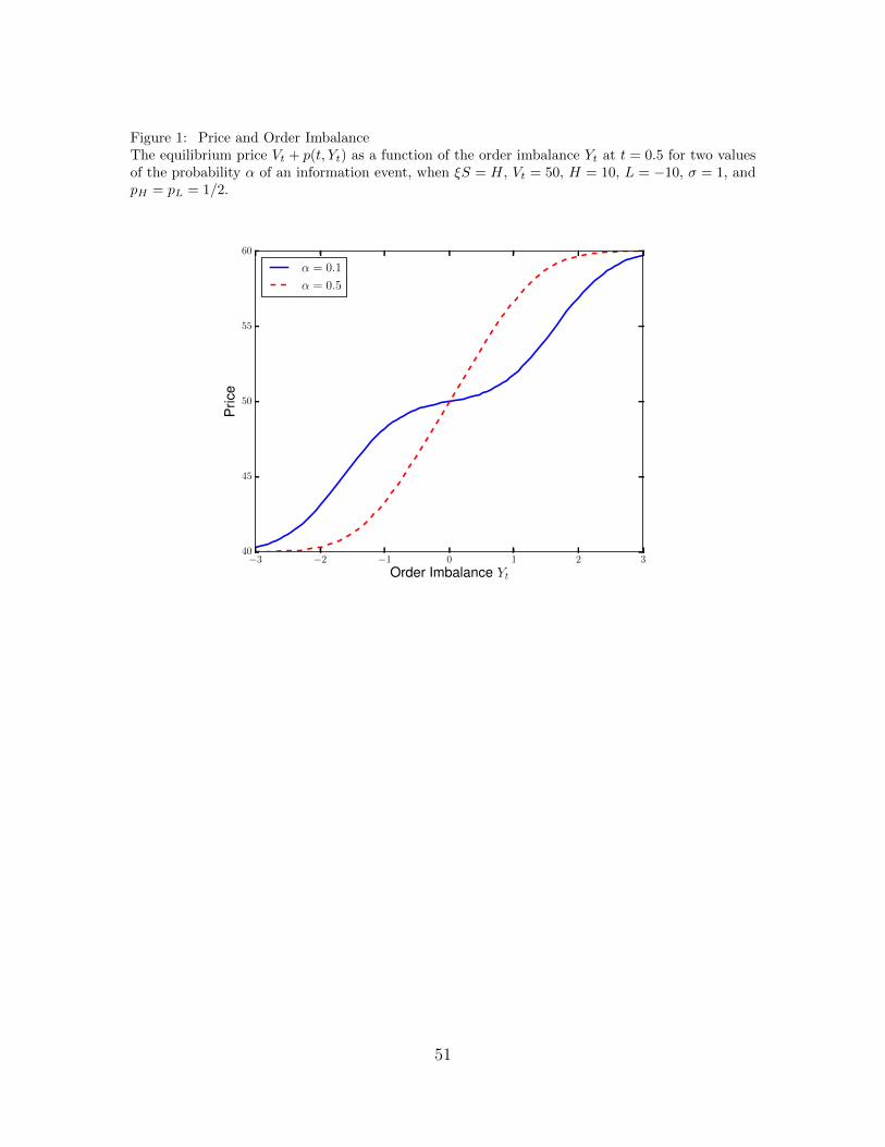
Figure 1: Price and Order ImbalanceThe equilibrium price Vt + p(t, Yt) as a function of the order imbalance Yt at t = 0.5 for two valuesof the probability α of an information event, when ξS = H, Vt = 50, H = 10, L = −10, σ = 1, andpH = pL = 1/2.
−3 −2 −1 0 1 2 3
Order Imbalance Yt
40
45
50
55
60
Pric
e
α = 0.1
α = 0.5
51

Figure 2: Expected Average LambdaExpected average lambda (8) as a function of α for two different values of H − L, taking |L| = H,when σ = 1 and pL = pH = 1/2.
0.0 0.2 0.4 0.6 0.8 1.0Probability α of an Information Event
0.0
0.2
0.4
0.6
0.8
1.0
1.2
1.4
1.6E
xpec
ted
Ave
rage
λ(t,Y
t)
H − L = 2
H − L = 4
H − L = 2
H − L = 4
52

Figure 3: Time Series of Hybrid Model EstimatesThe annual cross-sectional mean and 25th and 75th percentiles of parameter estimates for thehybrid model. The model is estimated on a stock-year basis for NYSE stocks from 1993through 2012 using prices and order imbalances in six hourly intraday bins and at the close.The model parameters are α = probability of an information event, κ = signal scale parameter,σ = standard deviation of liquidity trading, δ = volatility of public information, and pL =probability of a negative event. Expected λ is the expected average lambda λ(0, 0) based on Equa-tion 8.
(a) α (b) κ
(c) pL (d) σ
(e) δ (f) Expected λ
53

Figure 4: Time Series of PIN Model EstimatesThe annual cross-sectional mean and 25th and 75th percentiles of parameter estimatesfor the Easley et al. (1996) model. The model is estimated on a stock-year basis forNYSE stocks from 1993 through 2012 using daily buys and sells. The model parame-ters are α = probability of an information event, pL = probability of a negative event, ε =Poisson intensity of uninformed trades, µ = Poisson intensity of informed trades, and PIN =Probability of informed trade.
(a) α (b) pL
(c) ε (d) µ
(e) µε (f) PIN
54

Figure 5: Time Series of Price Impact EstimatesThe annual cross-sectional mean and 25th and 75th percentiles of percent price impacts. Five-minuteprice impacts are estimated daily and averaged annually for each stock-year for NYSE stocks from1993 through 2012.
55

Figure 6: The equilibrium informed trading rate θt as a function of the price Vt + p(t, Yt) at t = 0.5for two values of the probability α of an information event, when ξS = H, Vt = 50, H = 10,L = −10, σ = 1, and pH = pL = 1/2.
40 45 50 55 60
Price
0
2
4
6
8
10
Inte
nsity
θof
Info
rmed
Trad
e
α = 0.1
α = 0.5
56

Figure 7: Conditional Order Imbalance DistributionsThe density function of the net order flow Y1 conditional on a low signal, no information event,and a high signal for two values of the probability α of an information event, when σ = 1 andpL = pH = 1/2.
−4 −3 −2 −1 0 1 2 3 40.0
0.5
1.0
1.5
2.0
2.5Information Event with Low Signal
α = 0.1
α = 0.5
−4 −3 −2 −1 0 1 2 3 40.0
0.5
1.0
1.5
2.0
2.5No Information Event
α = 0.1
α = 0.5
−4 −3 −2 −1 0 1 2 3 40.0
0.5
1.0
1.5
2.0
2.5Information Event with High Signal
α = 0.1
α = 0.5
57
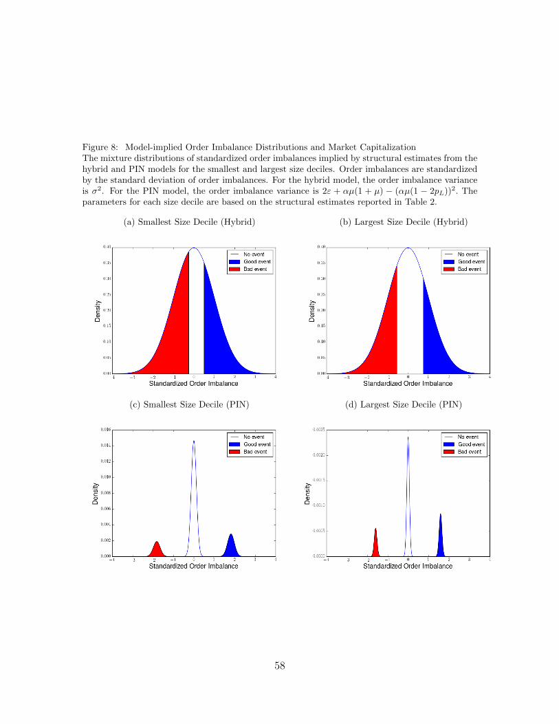
Figure 8: Model-implied Order Imbalance Distributions and Market CapitalizationThe mixture distributions of standardized order imbalances implied by structural estimates from thehybrid and PIN models for the smallest and largest size deciles. Order imbalances are standardizedby the standard deviation of order imbalances. For the hybrid model, the order imbalance varianceis σ2. For the PIN model, the order imbalance variance is 2ε + αµ(1 + µ) − (αµ(1 − 2pL))2. Theparameters for each size decile are based on the structural estimates reported in Table 2.
(a) Smallest Size Decile (Hybrid) (b) Largest Size Decile (Hybrid)
(c) Smallest Size Decile (PIN) (d) Largest Size Decile (PIN)
58

Figure 9: Empirical Order Imbalance Distributions and Market CapitalizationThe distributions of daily standardized order imbalances for the smallest and largest size deciles.For each firm-year, daily order imbalances are standardized by the firm-year standard deviation.The hybrid model is estimated using order imbalances measured in shares (top row) and the PINmodels are estimated using order imbalances measured in number of trades (bottom row).
(a) Smallest Size Decile (Empirical Shares) (b) Largest Size Decile (Empirical Shares)
(c) Smallest Size Decile (Empirical Trades) (d) Largest Size Decile (Empirical Trades)
59