ED 163 827

AUTHORTITLE

'INSTITUTION. PUB DATENOTEAVAILABLE FROM

HORS PRICEDESCRIPTORS

DOCUMENT RESUME'

_HE 009 936

Horch, Dwight H.Estimating Manageable Educational Loan Limits forGraduate and Professional Students.Educational Testing Service, Pkinceton, N.J.Mar 7850p.; Reproduced from best copy availableEducational Testing Service, Princeton, N.J. 08541

MF-$0.83 HC-$2. 06.Plus Potage.*Calculation; *College Students; *Financial Support;Graduate Students; Higher Education; *IncomeContingent Loans; *Loan Repaymen; Medical Students;Professional Education; Statistical Data; *Student*Loan Programs

IDENTIFIERS Law .Students

ABSTRACTEducational loin limits for graduate and professional

students were estimated*to provide manageable repayments that were aproportion of the borrowers' future consumption budget data. Based oneach professional group's -income profile, loan repayments werecomputed for each year.of repayment and summed across alternativerepayment periods to arrive at the aggregate ability to repay duringthe repayment period. Manageable aggregate ability to repay for eachgraduate and professional group was then converted into manageableloan principal limits for loans with alteriativeinterest rates,amortization periods, and repayment plans (equal installment andgraduate repayment option). The simulated manageable educational debt(levels were intended .to illustrate .the relationship' between thehypothetical prospective income of selected professional groups andtheir theoretical ability to repay educational loans. Borrowers maywant to.elect.a graduated repayment option and to extend therepayment period from 10 to .15 yea.rs if their total educationalindebtedness exceeds a threshold amount. Separate borrowing limitsand graduated repayment option plans could be established under,theGuaranteed Student Loan Program for borrowers in differentprofessions. Simulated loan principal limits pere'run for the'following groups: males with five or more years of college,. lawstudents, medical students, and doctoral scientists and engineers.Eleven tables and formulas for estimating loan repayments areincluded. (sin

***********************************************************************Reproductionesupplied by EDRS are the best that can be made

from the original document.***********************************************************************

.

b

me

At

Vor'e, ) I "r7:77:77777

ANA

N.

U.S. DEPARTMENT OF HEALTH.EDUCATION WELP AgeNATIONAt. INSTITUTEOP

EDUCATION

TINS DOCUmENT HAS SEEN REPRO-DUCRD EX,A411:Y AS RECEIVED FROM

THE PERSON OR ORGANIZATION ORIGiN-ATINCrIT. !POINTS Of VIEW OR OPINIONS

...ITATED DO NOT NECESSARILY R BITE-SENT OF Float. NATiONALINSTITUTEOSEDUCATION POSITION OR POLiCy.

;

5

e--

"PERMISSION TO REPRODUCE THISMATERIAL HAS, BEEN GRANTED BY

E1511CATIONAL TESTING SERVICE PRINCETON, NJ 08541

2

TO THE EDUCATIONAL RESOURCESINFORMATION CENTER (ERIC) ANDUSERS OF THE ERIC SYSTEM," ot.

0

4

Estimating Manageable Educational

Loan imits

for Graduate and Professional Students

Dwight H. Horch:;Program.Director

Graduate and FroTessional Scholia

Financial Aid Service

March 1978

It

6t1

4t

1 41Eduicational Testing Service, Princeton, New Jersey o.,e

e

. I

1

e.00

/ .0,

4

(4r.

O

c4.

ABSTRACT OFESTIMATING MANAGEABLE EDUCATIONAL LOAN LIMITS

FOR-GRADUATE AND PROFESSIONAL STUDENTSn'

Author: Dwight H. Horch, Educational Testing Service, Princeton) New Jersey

.

The main purpose of this study was to estimate educational loan ito.:14s for.graduate and professional otudents, which 'would result in a theoreticallymanageable, or comfortable, repayment stream.

Manageable repayments were defined as a proportion of.borrowers' futureincomes. The proportion of income which could be comfortably devoted to payingoff educational loans was estimated, from Bureau of Labor Statistics ;(BLS)cosumption budget data, to range from 5.4 percent of after-tax income at theBLS lower budget standard, to abOut 6.5 percent at the BLS intermediatestandard, and to almost 12 percent of after-tax income at twice the BLS higherbudget standard.

-Repayment formulas Were derived from BLSapplied to projected future income profilescians,..doctoral scientists and engineers; andmore-years of education beyond high schoo

- profile, manageable educatidnal loan repaymerepayment, and'summed across alternative repaggregate ability to repay during the pay-back

consumption budget data, and werefor samplings of lawyers, physigenerally for males With five or

Based on each group's income:s were computed for each year of.yment periods, to arrive at theperiod. 4

Manageable aggregate ability to repay for each graduate and professionalgroup was then converted into manageable loan principal limits, for loans withalternative interest rates, amortization periods, and repayment plans- -- equalinstallment and Graduated Repayment Option (GRO).

Based on Bureau of the Census profiles of average (mean) income by age formales with 5 or more years of education beyond high school, the manageableeducation 1 loan limit for a7 percent Guaranteed Student Loan (GSL) repayablein equal cstallotents over 10 years was estimated to be $7,100. Scalingrepayments to income, and extending the repayment period to 15 years increasedthe estimated manageable GSL limit to, between $16,000 and $18,900, if the

future inflation is between 3 oercent and 6 percent annually.

Because of differences In earnings prospects for the selected professionsincluded in this study, manageable eduCational loan limits differed, by profes-sion for repayment plahs graduated to.prospective income. This f*nding.impliesthat many heavily indebted borrowe'rs entering the profession -may be betterserved by Graduated Repayment Option (GRO) plans, because of/the young profes-sionals' relatively modest starting salaries and because of the comparativelyrapid rise in their income generally anticipated during the latter 'years ofrepayment.

The study draws upon income profile data that/were readily available fromprevious studies by other researchers. As a result, the simulated manageableeducational debt levels are Intended to illustrate the relationship between thehypothetical prospective income of selected professional Rroups and theirtheoretical ability to repay educational loans.

/

//'

/4

Several implications of he study are discussed. First, considerationshould be given to allowing borrowers' to elect a Graduated Repayment Option(GRO)_ and to Wend the repayment period from 10 to 15 years if their totaleducational indebtedness exceeds a threshold amount. The study also suggeStsthat separate borrowing limits and Graduated Repayment Option (GRO) plans couldbe established under the Guaranteed Student Loan Program for borrowers in

different professions.

While loans are seen as an important instrument for financing graduate and'professional education, the author suggests the importance of avoiding exces-sive reliance on loans at the graduate and professional level to the exclusionOf finahcial aid programs designed to foster equal access, intellectual excel-lence, and experiental work-study learning opportunities.

4.

t

.1

NTENTS

Page

Introductio' 1

Manageable educational"DebtI3 3

Conversion of Cumulative R. from Fudure IncomeStnto141an principal Linda 14

1Manageable,Educationai Loa

Limits or Selected Pro

aymentsnageable

Males 41th 5 or more ye1

Law' Students

11

Medical Students

PrinCipal"essional Groups

rs of'college

.19

Scien and Engineering

tStudents

Major4 indings and Policy

AnnendicJs. ,

1,,Appendix A:.

I.

1

Appendix B:

il Appg dix C:

i1

Appendix D:

1

21

23[.

V24

Implications 24

Formulas for E stimatingManageable'EducationalLoan Repayments

Income of Lawyers

Professional .Income ofPhysicians

IncPmesof DoctoralScientists and Engineers

PA%

27'

3

33

36

a

A

0

Table 1.

3*.

.1:ist of Tables

_Three Annual Budgets,for an UrbanFamilrof,Four, Autumn 1976'

Page

Table 2! Housing and Other Consumption' ExpensesExpressed as Percentages of AdjustedConsUmfttion Expenses at Three Levelsof Living, Autumn 1976

Table 3. Formulas for Estimating ManageableAnnual Educitional Debt Repaymentin Autumn 1976 Dollars

e.

Table 4. 'Estimated Mean.Incbme at Present ggee7and AgEarnings Ratios for Males

with Five Years or More ofPostsecondary Education

Table 5. Actual and Projected RisesAn the-Consumer Price Index <CPI):1972 to 1983

Table 6. Estimated Earnings profiles andManageable.Educational Loan Repaymentsfor Males with Five Years or Moreof College.,

Table 7 Formula for.Computing Total PrincipalGiven Monthly Repayments (IncludingPrincipal and Interest), Interest Rate:and Repayment 'Pe'riod

Table 8. Formula Denominators by AmortizationPeriod and Interest Rate

6

11

13

Table 9. Conversion of Manageable Repaymentsinto Total Manageable Loan, Principalfor Alternative Amortization Periods,at 7% Interest, for Males with 5 orMore Years of Postsecondary Education 17

.

Table 10. Estimated Manageable Cumulative t

Repayments (Principal andApterest),by Amortization.. Period for Selected,Professional Groups 20

15

15

Table 11. Estimated Aggregate Educational LoanPrincipal Borrowing Limits,for EqualInstallment and Graduated RepaymentOption (GRO) Plans for SelectedProfessional Groups .... .. 22

7A

J

4

[Introduction

Educational. loan programs have become a major instrument over the past twodecades for financing postsecondary educational costs. Iii retrospect, theinitial appropriation of $60 million in fiscal year 1959 for the National DirectStudent Loan Program, the only federal loan program in its time, seets triflingin contrast-to current borrowing levels, which approached $1.85 billion for themyriad,pf fedefal loan programs in fiscal year 1976.

. .4

Loan programs have evolved over the years in.response to increasing coatsj at both the undergraduate and post-baccalaureate levels and to perceiyed

needs and political pressures. The National Defense Student Loan Program(NDSL), for example, was created in the post-sputnik era to accelerate_post-secondary training. The Guaranteed Student Loan (GSL) Program, on the other. -hand, was enacted to ease the financial burden of college,costi on middli income''families, as an alternative to tax credits. Other loan programs on thefinancial aid laddscape include `the Nursing Loan Program, the V.A. EducationalLoan Program, and the Health tduCation Assistance Loan (HEAL) Progiam forprospectiviihysicians.

The importance of loans is underscored by the fact that some $1.3 billionwere borrowed in 1976 by students through the Guaranteed and Federally InsuredLoan Progrgms. On an, individual basis it is reflected in average borrowings ofstuents, which can only be expected, to increase in the future.. A recentsurvey of 70,000 postbaccalaureate students in the 1977-78 Graduate and Profes-sional School Financial Aid Service population, revealed that almost one-half(47 percent) reported they had borrowed some amount.during their undergraduate.years. And for those unmarried students who had borrowed, the median cumu1,lveeducational debts were a's follows:

01*

Year in Graduate/ Median CumulativeProfessional School Educational Debt

First

Second' A

Thir4

Fourth

$ 2,684

$ 3,709

$5,458

i$ 7,899,

1

2

John F. Morse., "How We Got Here from There A Personal Reminiscence of theEarly Days` in Student Loans: Pnobiems and Policy Alternatives. CollegeEntrance Examindiion Board, NeW York, 1977, p. 13.

D.H. Horch, "Need Analysis at the Graduate and Professional Level: Who

Needs It"? Paper prepared for the Student Loan Marketing Association Symposiumon Financing Graduate and Professional Education, June 1977, p. 53.

0

- 2. -

While these debt loads are not particularly alarming, the level of indebt-edness may be expected to increase in the future, for aAvariety of reasons.Hough notes, for example, that the demand for loans., especially by graduate andprofessioqal students, is likely to, rise, despite projected future enrollmentdeclines.

Hough arrives at this seemingly contradictory conclusion thrqugh thefollowing logic chain. As the flow of high school graduates begins to decline,enrollments in institutions ot higher education may also be expected to decline.This will create_, an upward push on tuitions, to the extent that the volume bfstudents declines and the fixed cost base for tenured salaries remains,constant.

As costs escalate, pressures toward debut financing Will mount at thegriaduate and professional level ln.the absence of government.intervention in ,theform of uncategorical grant assistance to institutions or grant assistance tostudents.

There is a growing concern. that increasing. debt burdens will create in-creasingly serious/repayment problems for students 'in the future, and may have.Aiittende4 pervasive consequences --.such as income maximization behavior of,borrowers -- that may conflict With broader social goals.' For example, Congressrecently enacted .the Health Education Assistance Loan Program with a maximumaggregate loan limit of $50,000, an (unsubsidised) 10 to 12 percent interestrate, and a 15 year_ repayment period. While it can be argued that the incomeprofiles of physicians permit absorption.of this level of indebtedness, it-canalso be hypothesized that heavily indebted physicians may opt for practicesinmore'lucrative nonshortage areas. Another possible consequence of high debt iq'ikvein for physicians is. a further upward push on their-professional fees.Similar types of behavorial consequences of borrowing can be hypothesized forother professions, such as law or' business.

The growing importance of loans)as an instrument for financing graduate apdprofessional study, and the concerti over the repayment legacy they entail,suggests the need to devetfp a Methodology for estimating loan limits that arenot overly burdensome.

:he balance of t'bis paper is devoted to developing alternative definitionsOf manageable loan limits, and simulating loan limits for borrowers in electedprofessions! Because of the key role loans are likely to play'in the yearsahead at the postbaccalaureate lIvel, this study is restricted to estimating

4manageable loan limits for graduate and.professional students.

3Law

,

rence A. Hough,6

Introduction to Student Ln Marketing AssociationSymposium on Developments in Finncing Graduate .Educition. :

.

J4

.s

Manageable Educational. Debts

The question of what constitutes a manageable education debt level has beena vexing one, and, 'as JOIstone points out "there is little on which to base ananswer to the. question." There seems, to be agreement, however, that therelevant measure of the "oppressiveness of a debt is the relation between futurepayments and future income. At some level, the ratio of annual repayments toannual income becomes burdensome."

Perhaps the most definitive work in the area of tolerable educational debtlevels was undertaken by Daniere in the 1960s.6, Daniere examined consumerexpenditure profiles and concluded that families spend about 90 percent of theirafter-tax income for.consumptionleaving a residual of 10 percent. A priori,he concluded it would be unreasonable to expect borrowers to devote,all of theirresidual income for educational debt repayment and\saggested that 6 percent ofbefore-tax income, or 7.5 percent of after-tax income, could be devoted to,retiring educational debts, without being overly burdensome.

t

Daniere concluded that a tolerable educat,ional loan would be defined as oneentailing annual repayments equal to, or less than 7.5 percent of an individ-ual'i* after-tax income.

Hartman, following a different reasoning,.concluded that up to 15 percentof the typical college graduate's starting income, before taxes, would not be anoverly7burclensoine educational loan repayment, assuming equal annual install-ments. He based his conclusion on .the assumption that during the paybackperiod students might be willing to accept a level of repayments equal to theincrease in their earning power resulting from a college education.

Froompkin, in his study of student loans for women,8used three teets.of

repayment burdens to evaluateloan'repayment plans:- f

4Bruce D. Johnstone, New Patterns for College Lending, Columbia Universitypress, New York and London, 1972, p. 106.

5Robert W. Hartman, Credit,for College, New York: McGraw Hill, 1971,.p. 14.

.6Andre- Daniere, "The Behefits and Cps of Alternative Federal Programs ofFinancial Aid to College Students," in The Economics and Financing of HigherEduCation in the United States: A Compendium of Papers Submitted to the Joint.Economic Committee (Washington, U.S. Government Printing Office, 1969),pp. 576-578.

7Hartman, op cit, p. 19.

8Joseph Froomkin, Study of the Advantages and Disadvahtages of Loans to Women,Prepared for'the Department of Health, Education, and Welfare, Decembe'r 1974;Distributed by National Technical Informatioi Service, U.S. Department ofCommerce,p. 14.

- 4 -

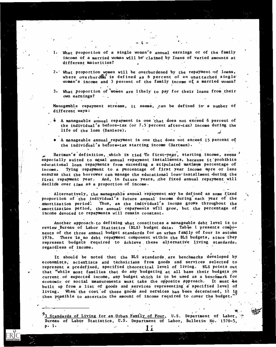
1. What proportion of a single woman's annual earnings or of the familyincome of a married woman will be'claimed by roans of varied amounts atdifferent maturities?

2.- What proportion wren will be overburdened by the repayment 'of loans,where overburden is defined as 6 percent of an unattached single'woman's income and 3 percent of the family income of a married woman?

3. What proportion of'woMen are likely' to pay for their loans from theirown earnings?

Manageable repayment streams, it seems, ,can be defined in a number ofdifferent ways:

A manageable annual repayment is one 'that does not exceed 6 percent ofthe individual's before-tax (or 7.5'percent after -tax) income during thelife of the loan (Daniere).

A manageable annual repayment is one that does not exceed15 percent ofthe individ'ual's before -tax starting income (Hartman).

Hartman's definition, ,which is tied to first-year, starting income, seemsespecially suited to equal annual repayment installments, because it'prohibitseducational loan repayments from exceeding a stipulated maximum percentage ofincome. Tying repayment to a percentage of first year income more or lessensures that the borrower can manage the educational loan-installment4uring thefirst repayment year. And, in future years, ithe fixed annual repayment willdeclide over time as a proportion of income.

Alternatively, the manageable annual 'repayment may be defined as some fixedproportion of the individual's future annual' income during each year of theamortization period Thus, as the individual's income grows throughout theamortization period, the annual repaymerits will grow, but the percentage ofincome devoted to repayments will remain constant.

Another approachto defining what constitutes a manageable debt level is toreview Bureau of Labor Statistici (BLS) budget data. TabJ1e 1 presents co4o-nents of the three annual budget standards for an urban faml.ly of four in autumn1976. There ls,no debt repayment component within the BLS budgets, since theyrepresent budgets required to Achieve, these alternative living standards,

regardless of income.

d

It should be noted that the BLS standards are benchmarks developed byeconomists; scientists and technicians from goods and services selected- torepresent a predefined, specified theoretical level of living. BLS points outthat "while most families that do any budgeting at all base .their budgets ,oncurrentor expected income, any budget which is to be used as a benchmark foreconomic or social measurements must take the opposite approach. It must bebuilt up from a list of goods and services representing a' specified level ofliving. When'the cost'of these goOdi and services has been determined, ii 1.0then popsible to ascertain the amount of income required to cover the budget."

I *1Vk

it*.°93 Standards of Living for an Urban Family of Four, U.S. Department of Labor,Bureau of Labor Statistics, U.S. Department of Labor, Bulletin NO. '1570-5,p. 1.

- 5

a

The BLS budget, standards do not imply that individual families at 'Specifiedlevels actually allocate their incomes in a manner necessarily consistent withthe components of the standards. Thus, to a lesser or greater extent, dependingupon the budget componentyand the standard, families have.some discretIon i/T1 howthey spend their incomes.

Table 1.' Three Annuarltudgets for an Urban Familyof sour, Anvmn .

Component Lower

a

Intermediate

r

Higher

*AI

Food

Housing

Transportation

.Clothing

Personal Care. . ,

Medical Care

-Othet Consumption'

Total Family, Consumption'

Other Items

Adjusted Consumption.

$3003-

1964

, 799

265

896

468

8162

451

$8612)

ii

. .

- ,

wFR .4(4199k

$3859

3843

1403'

1141

900

869

12370

731

$13101

_$4856

5821

1824

1670

503

939,

. 1434

117048

234

, $18282

'Other consumption includes average costs for- reading, recreation, tobacco;alcohclAic beverages, education, and miscellaneous expenses.

2Other items includes allowances for gifts And contribiltions, ,lit_inauranceand. occupational expenses. ,k

ourc Monthly Labor Revi'ew, July 1977, p. 35

I

?N.

r

0

v. -1 I

&rev ew o f the BLS standards In able 1 reveals two-components that appearto be largely discretionary-- - "other co sumption" and "other items." While thesecould be viewed as discretionary amounts which could be .allocated entirely to .

annual educational .debt amortization, such, an assumption could conceivablyrequire major budgeting dislocat S on the part of the family. .0n the otherhand, it can be argued that ount approximating the 'other consumptioncomponent of the respective bud s could theoretically be devoted to educe=tional loan repayments without c ating an undue strain on the family.budget.-Thus, manageable annual educational loan repayment could be defined aeonamount equivalent to the other consumptiop component of the respective BLSbudget staddards.

f-lbe data in Table 2 present housing and other consumption budget componetsexpressed as percentages of the three adjusted consumption budgets. At the BLSlower consumption budget standard, housing costs represent 22.8 percent of the.standard and other consumption items. represent 5.4 percent of the lowerstandard. Thedepercentages increase progressively to the intermediate andigher standards. Note the fact that the'other consumption component representsbetween 5.4 and 7:8 percent of the respective budgets, a range that encompassesDanieres 7.5 percent gigure.

FOr purposes of this study, manageable debt .repayment is defined' as anamount equivalent to the other consumption component of the respective BLSbudget standards. It.should be pointed out that the total adjusted consumption,:budgets in Table 1 .exclude federal, state, FICA and local taxes. As such; theyrepresent-income after taxes (effective income) needed to'achieve each of thethree budget standards.

4

Table 2. Housing and Other Consumption Expenses Expressed as Percentages ofAdjusted Consumptions Budgets at Three Levels of Living,Autumn 1976

Component Lower Intermediate Higher

Housing 22.8% 29.3% 31.8%

.Other Consumption

,Housing plus OtherConsumption

5.4% 6.6% 7.8%

28.2% 35.9% 39.6%4

If one accepts this definition, the question becomes, "Given a known annualincome, how can the annual manageable educational loan repayment be estimated?"

1°

Using the data in Table 4it-is osaibla tp, construct a progressiveschedule that, at each of the three budget -atelhdazds, yieldi expected annualrepayments equal to the Other Consumption component. For example, The'OtherConsumption component (or manageable repayment) represents 5.4 percent of theTower budget standard ($8,610), or $465. At the moderate standard, it is $869($465 from the lower standard -plus 9-'PecCent of the. difference between'theamount of the lower and the intermediate sxandards.).

, 0

Table 3 presents a progressive schedule.vhich.waa constructed to estimatepanageable debt repayment from 1976, effective income (income after teies3. At'double the BLS higher standard the.manageable annual repayment was assumed to bethree-times the repayment at the higher standard.

Table 3. Formulas for Estimating Manageable AnnUal Educational Debt Repaymentin Autumn 1976-Dollers, . .

Autumn 1976 .Manageable Annualeffective income (El) Educational Debt Repayment

. .

1

$ . 0- 8,610 - - 5.4% of El

$ 8,611-13,100 $465 plus' ET in'- 1 excess of

$

f $86..

13,101-18,280.

$869 plus 11.0% of El. in excess of $13,100 -

.

$ 18,281 -over $1,439 plus 15.7% of Erin excess of $18,280

f 4 _

I. Effective income = Adjusted gross income less allowance for U.S. income,taxes, FICA taxes, and state and other taxes. .

Effectively, the above formulas result in exptcting hollowing propor-tions of after-tax income for educational debt repayment: 5.4 percent attheBLS lower standard, 6.6 percent at the BLS intermediate standard, 7.9 percent atthe BLS higher standard, and 11.7 percent at twice he BLS higher standard.

,Since educational loans are repaid from thestudent's future income, theability to repay educational debts can be viewed as a function of the student'sfuture income stream during the amortization period. To estimate aggregatemanageable educational loan repayments for graduate and professional students,age-earnings profiles must be taken into considefation. The, Bureau of theCensus periodically estimates- the mean income, lifetime income, and educational.attainment of men in the United States. Oneof the groupings for which thesedata are available is for men with five years or more of college.

a

M

- .8

'Mean incomes for this group, in 1972 dollars,' are presented by age in Table4. This table reveals that the mean incOmesin 1972 dollars foi 26 year old menwith five. years or more of college was $11,104. The daps in the "ratio" columnpresent mean incomes at each age expressed as a ratio,Of the income for. therespective' age group to the mean income at the base age of 26. Age 26 was'chosen as the base lor,thie group because it is the earliest age at which themajority of 4graduatelprbfessional'borrowers in four year educational 'programswould begill repaying their'loane, swimming a grace period.

-

I

r

Aro

Tablelb4. Estimated Mean Income in 4972 Dollars at Present Age andAge-Earnings Ratios for Males with Five'Years or More oaf

Posxsecondiry Educatibn

Age Income

26 11,104t7 11,854

28 '12,577

29 11,27330 13,94131 14,58132 15,194

33 15,77934 16,33735 16,86836 9 17,37137 17,84638 18,29539 18,71540 19,10841 19,47442 19,81243 20,12344 20,40645 20,661

46 20,89047 21,09048" 21,264

49 21,40950 21,52851 21,618

52 21,68253 a 21,718

54 52,72655 21,707

56 21,66057 21,58(1

58 21,48559 21,35660 21,19961 21,01562 20,804'63 20,56564 20,298

Ritio

r

1.001071:131.201.26

1,,31

1.371.421.47

1.521.561.611.651.691.72

1.751.78

1.81

1.841.86

1.881.901.92

1.93

1.941.95

1.951.96

1.961.951.951.94

1.931.921.91

1.89

1.871.851.83

Source: Bureau of the Census, Current Population Reports,Series P-60, No..92.,

16

- 10-

.

/ i.0. The census dats/SuggeSythat income wirgrow (in 1972 dollars) as. a func-

tion of age by 7 peicent fr'm age 26 to 27, by 13 percent form age 26 to age44;and so on. Thefincome 9f males with five years or more of college may- beexpected to grow by 52 peAent petween ages 26 to 35 (first 10 years),`and by 86percent by the entiethiyearAage 45).

In measuring aggregate manageable debt repayments, which will be made fromfuture incOe, the impact of inflation on income should not bie ignored.Actordinglyi, the projection of furture income streams should accoliht for bothinflation 'and cross-Secti growth. 'onal income rowth. .

(..,

clitite 4rilable.htrefore, need to be'updati4Nto reflect inflationaryeffec from/19/2 t6 fuure/repayment years. Students .entering four-year degreeprogr "In LOT8-79..Nolild not be expected .to begin repayMent. of their loansunt the:beginiting of 1983. For this reason, ,the.-1972 census income data needto e ',update-a:through-A:983 for inflation. Actual andj projected Consumer PriceI ex (CPI)'/increases for ,the. period 1972 to 1983 are presented In Table 5.allied on the actual increase in the CPI from 1972 through 1976, and projected

./.2

ncresses through 1983, it is estimated that the .CPI will increase by 103.9percent for the period 1973 through 1983. Therefore, the average 1972 income of$.11,104 for a 26-year-old male with five or more years of college, when updated

'.. for CPI - increases to 1983, becomes $22,641. Further, the average 1972 before-

/ tax income of $16,337 for a 34 year old would grow to $53,092 in 1991, assuminginflation of 103.9 percent from 1972 to 1983, and a 6 p ercent rate

/'thereafter. Long-range estimates of rises in the CPI are subject to consider-able uncertainty. Therefore, for purposes of estimating manageable debtrepayments from future income streams, it might be preferable to assume a lowerrate of inflation. This would result in the yielding somewhat more Conservativeestimates of ability to repay from future income streams.

k

0

Table 5. Actup and Projected Rises in the Consumer Price Index (CPI):% '1972 to 1983

.

' Percent IncreaseYear C _ - (1972 =Base)

.

19721

12 .3

19761/_

0.5"... .

19772 . ;181..6

.19.0 192.1'10

1979 202.7 -

1980 213.8

1981 \____ 228.4 ,

/ 1982, 24 i,

92.3%

1983 255.5 : 7 103.9%

1Source:- Monthly Labor Review, August' 1977

.

2Source: Data ResourCes Inc. Predictions Of National 14iCe. and Wage

Increases. h

Table 6 presents estimated earnings profiles and managale annual andcumulative educational debt repayments for 10 and 15 year amortization periods,assuming repayElents begin in 1983 For this analysis, the census age-incomeratios for males were assdmed to be representatlive.of earnings profiles for theuniverse of graduate and professional: students.,

10-10 the extent that there may be significant differenceS in starting salariesand age-income ratios (growth profiles) among students in various disciplinesand between men and women, one would 'expect manageable debt loads to varyamong disciplifiespand occupations and between sexes. Moreover, to the extentthere may be differences in' cross sectional income growth rates among racialand ethnic groups, different manageablsdebt loads would be implied by theapproach.

0

- 12.(1.-

!\

Wite that.mandAble annual debt repayments were computed for each yearI

\

usin the "effective" or after -tax .income formulas presented in Table 3, updated.for inflation. Just as inflation of income neeeds to ,be accounted for, so toodo nflationary impacts on the repayment formillas them Ives. Formulas forleachfut e! year were, therefore, indexed for inflation. Effective income wasdefineS:as adjusted annual income'(i.e., adjusted for inflation and age growth)

i

les tie- sum of estimated federal income paxes, PICA taxes and state and othertax s' The alIowance'for state and other/taxes is 8 percent of adjusted income,the aiount alLowed by. uniform methodology fianancial need analysis proceduresort famlieq whose total income exceeds $10,000.

..,

qty

J)11See Appendix A, formula 3, which was used to index the annual repaymentschedule.

tic

4

/

- 13 -

Table 6.r . . .

E4timated Earnings Profiles and Manageable4nnual EducationalLOan Repayments for Males.with)Five Years or More of College,A.61uming 6 Percent Inflation After 1983

!

...

. I Before TaxLoan`Repaymerit 'Income in 2

:Year ' 1972 Dollars

(1) 1983. r

(2) 1984

(3) 1985

(4) 1986

(5) 1987

(6) 1988

(7) 1989,

(8) .1990.

(9) 1991

(10f 1992

(11) 1993.

(12) 1994

T'(13) 1995

(14) 1996

(15) 1997

111,104

11,854,

12,577

13,273

13,941

14,58i

15,194

) 15,779

16,337

,16,868

17,371

17,846

18,295

18,715

19,108

After Taxin .

Current Dollars

ManageableAnnual LoanRepayments

CumUlativeRepayments

$16,127

18,003

988

1%129 ,

.19,795 1,261

210403 1,410

23,720 1,550 A

25,,543 1,679

27,560 11823%,-

29,510 1,96610 Year

- \--31,626 2,122 Amortization($16,221)

33,921 2,293

c)36,218

t...,

2,00

38,902 2,663

41,594 2,862 . 15 YearAmortization

44,500 3,079 30,575

47,396's 3,289

1Assumes entry into a four-year graduate/professional program in 1978 -7.9,

exit age 25 in 1982, nine month grace period, and repayments.beginning in1983. .

2Souce See Table 4.

3Assumee 103.9 percent rise in CPI from 1972 to 1983, and six percent annualincreases thereafter in before-tax Income. After-tax income equals incomeless allowances for federal taxea, state and other taxes, and FICA taxes.

2C

44'

' - 14'1

J

The far right column of Table 6 presents the.cumulative manageable repay-ments at the tenth and fifteenth years. The outc6mes of this analysis suggestthat, 'given a 10 year AFayment period, aggregate repayments,,igraduated toincome, of $16,221 would be manageable; given a 15-year

12mortization period,

4"..aggregste repayments of $30,575 .would be manageable. It is extrImelyimportant to note that these statements assume annual repayments are sceled toincome and 'an inflation rate of 0 percent. Without such scaling, the studentamortizing a loan in equal installments Could be expected to repay more than amanageable amount during the first years of repayment.

The chart on the next page illustrates the ability of selected professionalgroups.to make annual educational loan repayments over a 15 year amortization

(4. period. The chart demonstrates, on average, little difference in ability torepay educational loans of doctoral scientists and engineers, and males with 5or'mOre 'years of college. Moreover, the ability of lawyers and physicians torepay educational `loans is not markedly different, if-physiciani-by required tobegl.n repayments during internship and residency. Not surprisingly, ifphyeicians are permitted to begin repaying educational loans afterythe residencyperiod they appear-as a group, to theZreti6ally have the ability to make thelargest annual" repayments.

4Conversion of Cumulative Repayments from Future Income into Manageable LoanRrincipal. LiMits

In.thepraceding section, a methodology was presented for measuring manage-able. aggregate educational loan -repayments as a function of future incomeprofiles for a group that may approximate graduate and professional students asa whole.

Having presented this methodology, the question becomes, "What is theaggregate tolerable loan principal (as opposed to repayment), given manageableaggregate repayments?". Naturally, to answer this question, the repayment periodand the interest rate must bq stipulated, because repayments include bothprincipal and interest.

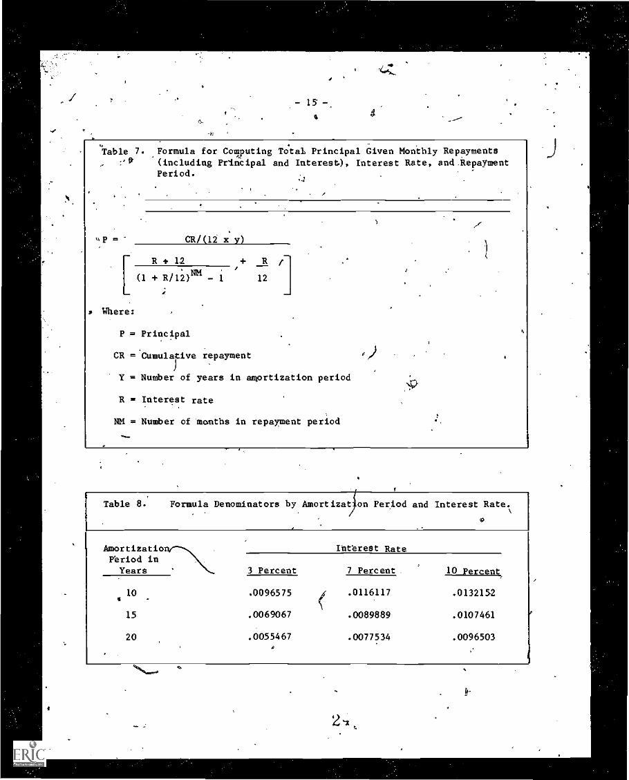
Table 7 presents aggneral formula for computing total 'principal, givenmonthly repayments, interest rate, and number of months in the repayment period.Table 8 presents denominators for the formula for different repayment periodsand interest rates.' Table 9 converts the cumulative manageable repaymentsdeveloped in Table 7 into total tolerable _debt principal for a 7 percentinterest - bearing loan repayable in LO or 15 years.

12Formulas' 1-4 of Appendix A wererepayments.

used to determine cumulative manageable

EeiMATED MANAGEABLE GRADUATED EOCATIONAL LOAN REPAYMENT

- IS

I

. ,

Table 7. Formula for Computing Total Principal Given Monthly Repayments:'$ (including Principal and Interest), Interest Rate, and.kepayment

up in

Period.

CR /(12 x y

R + 12 + R

(1 + R/12)11K - 1r

12

s Where:

P = Principal

CR ='Cumularive repayment

Y = Number of years in amortization period

R = Interest rate

NM = Number of 'months in repayment period

ti

Table 8. Formula Denominators by Amortizat on Period and Interest Rate.

Amortizatioftriod inYears

Int'erest Rate

3 Percent 7 Percent. 10 Percent

10

15

20

.0096575

.0069067

.0055467

.0116117

.0089889

.0077534

.0132152

.0107461

.0096503

- 16 -

The data in Table 9 suggest that repayments of $16,221 would be manageableiover a 10 year.amortizati6atperiod ior a loan bearing 7 percent interestconverts into a loan principd1 of $11,641. Stated differently, the analysissuggests that an aggregate loan limit of $11,641 for the universe of graduate.and professional students, may be a manageable loan 'ceiling fora '10 yearamortization period, assuming repayments are scaled to future income. If theamortization period is extended to 15 years,, it appears that a $18,896 loanprincipal ceiling, would be tolerable.

The aggregate loan (principal) limit for the Guaranteed Student LoaneProgram (GSLP) was recently extended to $15,000 for griaduate and professional

students. This analysis suggests that the$15,000 limit is not unreasonable,provided the 10 year amortization period is extended tct_15 years and repaymentsare graduated or scaled to income. Given a fixed repayment schedule and a tenYear amortization period, one could argue that the total debt repayment shouldnot exceed 10 times the manageable repayment during the first year of repayment.If the required equal monthly installment exceeds the manageable monthly repay-ment the first year, one might hypothesize that undesirable personal and socialconsequences, such as default, might Ault. Following this line of reasoningfor the example in Table 6, a manageable aggregate GSL loan principal limit formales with 5 or more years of postsecondary training, given an equal monthlyrepayment schedule, would be about $7,100.

$988 x 10 yrs. 4. :01161`I7 = $7,090120 months

r-

The preceding example highlights the imporilice of permitting graduate andpfofessional GSL Program borrowers the option of graduated repayments, andsuggests that the amortization period should be extended to 15 years for thoseborrowing in.excess of $7,100. Referring back to the.manageable annual repay-ment column of Table 6, it appears that annual GSL repayments, if graduatedto allow approximatelx a doubling of annual payments from the first to the tenthyear of repayment or 'a tripling from the first to fifteenth year, would resultin a manageable repayment stream for males with 5 or more years of postsecondaryeducation.

-

- 17 -

.

Table 9. Conversion of manageable repayments into total manageable loan

.."---...principal for alternative amortizaxion periods, at 7% interest,

yfor males with5 or more years of postsecondary education.

(Assumes 6 percent inflation after 1983)

71

. . 10 Years - 15 Years,.

Itemi

(120 Months) (180 Months).. .

Total Manageable.Repayment . $16,2211 i $30,575

1

. .4

(

Average Monthly"

Repayment $135.18 $169.86.

.

Formula Denominator .01161172

. .00898892,.

.

s

Total Manageable3

Loan Principal $11,64 I '$18,8963

I I1Sourpe: Table 6 k 1..

N.2Source: Table 8 (

.

3as follows: Montly repayments divided by formula denominator.'

o (

Th= preceediUg example reveals that several variables impinge upon theassess nt oaf manageable educational loan principal limits:

Length of the amortization period

- Interest' rate

Shape pf ehe=oge-income profile

Burned inf*Otion rate in future years

Equa installment or graduated repayment option (GRO) schedules

Starting

*-1

;k:

- 18-

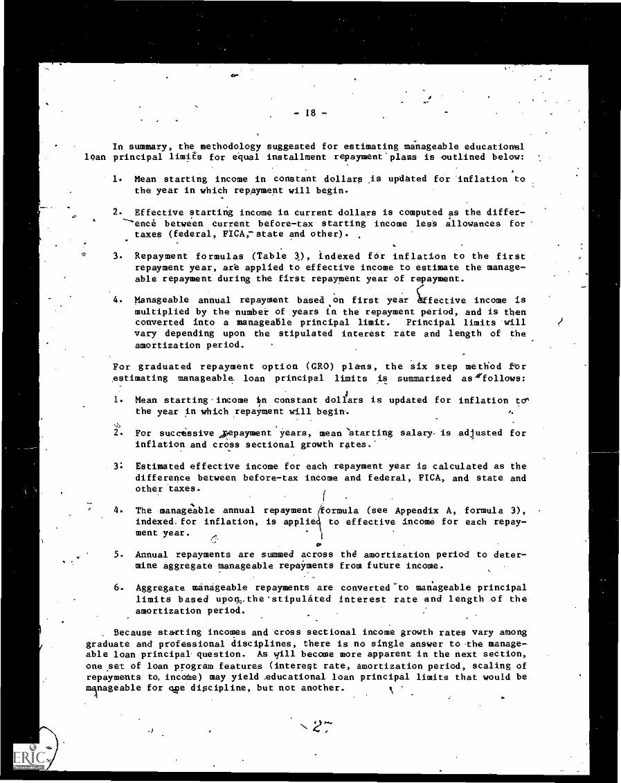
In summary, the methodology suggested for estimating manageable educationalloan principal limits for equal installment repayment'plaas is outlined below:

1. Mean starting income in constant dollars As updated for 'inflation tothe year in which repayment will begin.

2. Effective starting income in current dollars is computed as the differ-pence between current before-tax starting income leas allowances for

taxes (federal, FICAi-state and other).

3. Repayment formulas (Table 3), indexed for inflation to the firstrepayment year, are applied to effective income to estimate the manage-able repayment during the first repayment year of repayment.

Manageable annual repayment based on first year ffective income ismultiplied by the numbei of years in the repayment period, and is thenconverted into a manageable principal limit. Principal limits willvary depending upon the stipulated interest rate and length of theamortization period.

For graduated repayment option (GRO) plans, the six step method barestimating manageable. loan principal limits is summarized as.'rfollows:

1. Mean startingincome itn constant dollars is updated for inflation to"the year in which repayment will begin,

2. For successive , epayment Years, mean 'starting salary- is adjusted forinflation and cross sectional growth rates.'

3; Estimated effective income for each repayment year is calculated as thedifference between before-tax income and federal, FICA, and state andother taxes.

I4. The manageable annual repayment formula (see Appendix A, formula 3),

indexed. for inflation, is applie to effective income for each repay-went year.

1

5. Annual repayments are summed across the amortization period to deter-mine aggregate manageable repayments from future income.

6. Aggregate manageable repayments are converted-to manageable principallimits based upon,,,the'stipulated interest rate and length of theamortization period.

Because starting incomes and cross sectional income growth rates vary amonggraduate and professional disciplines, there is no single answer to the manage-able loan principal question. As dill become more apparent in the next section,

one set of loan program features (interest rate, amortization period, scaling ofrepayments to, income) may yield .educational loan principal limits that would bemanageable for qea discipline, but not another.

- 19 -

Manageable =Educational Loan Principal Limits for Selected Professional Groups

To test the .sensitivity' of the methodology for estimating manageableeducational loan principal - limits, an interactive computer model was develdped.The model allows the user to stipulate the following variables: starting income

rin current dollarsg..age-income growth ratilis, inflation rate, interest rateandA

.number of /ears in the pay-back period. It then computes manageable educationalAebt.loads using the formulas tb Appendix A.

;

A series of simulations were, run to estimate manageable educational loanprincipal limits for each.of_51g following groups:

9- Males with or more years of college

Law Students

Medical students, assuming repayment begins during internship

Medical students, assuming repayment begins after residency

Doctoral'scientists and engineers.

' The simulations drew upOnincome.profile data that were readily availablefrom previous studies by other researchers.' In addition to simulations based on'Bureau of the Census data for males with 5 or more years of college, the simula-tions for lawyers utilized income profile dta published by the MassachusettsBar Association, those for doctoral scientists and engineers drew upon datapublished by the National Academy of Sciences; and unpublished income data froithe Institute for Demogrphic and Economic Studily were used to simulate mane eAble educational debt levels for physicians. As a result, the simulatmanageable educational loan limits are intended to illustrate the relaiionshbetween the hypothetical prospective average (mean) income of selected prof esatonal groups during the pay-back period and their theoretical ability to repaeducational loans. Because available income profile data for selectedprofessional groups may not be wholly representative, the reader is urged tointerpret the results,of the simulic.A.ons cautiouslA Similarly, because theestimates of manageable debt levels are based on group mean incomes at selectedages, the reader is cautioned against inferring that the results are necessarilyapplicable to individuals.

The results of. all of the simulations are highlighted in Tables 10 and11. Table 10 presents estimated manageable cumulative repayments, includingprincipal and interest, by type of repayment (fixed or graduated), for selectedpay-hack periods and professional groups. Inspection of Table 10 reveals that,for males with 5 or more years of college, total] repayments of $9,900 would betheoretically manageable, given a 10 year amortization period and restrictingcumulative repayments to 10 times the repayment, that is manageable from thestudent's income during the first year of repayment. On the other hand, if

annual repayments were scaled to income, the cumulative manageable repayment,given a 10 year amortization period would be between $14,700 (if the inflationrate were 3 percent annually) or $16,200 (if the inflation rite were 6 percentannually). 0

12The age - income profiles and estimated starting incomes for each professional,group may be iOund in Appendices B through E. A

is

.

Table 10. Estimated.Manageable CumulariVe Repayments (Principal and Interest) by Amortization period for Selected Professional Groups

AmortizationPeriod

4

Males with 5 or moteYears of College

. *Lawyers

' 11(1::::::::e

Beginning afterResidency)

Pysiciane(Repayments Beginning

in Internship)Doctoral Scientists

and Engineers

Equal GtaduatedRepay- Repay-sienna meats

Equal -Graduated. Repay- .Repay -

. men'e meats

Equal Graduated

Repay- Repay-meats meats

Equal GtaduatedRepay- Repay-meets mgnte

Equal Graduated

Repay- Repay -meets mental

10 Years

15a

Years

20 Years

'$9.9 $14.7-16.21

$14.8 $25.8-36.6

$19.8 $39.4-50.8

$8.9 $20.9-23.4

$13.4 $41.7-50.8

$17.9 $70.9 -95.7

$22.0 $39.1-44.2

$33.0'

$77.5-96.7

$44.0 $134.3-186.9

$10.4 $19.0-21.4

$15.6 $40.4-49.6

$20.8 73.9-101.8

$12.9 $16.7-18.3

$19.4 $28.3-33.4

$25.8 $42.8-55.1

'\

1 Lower limlt assumes 3 percent annual inflation rate; upper limit assumes 6 percent annual inflation rate..

., .

s.,' .

.

-21-

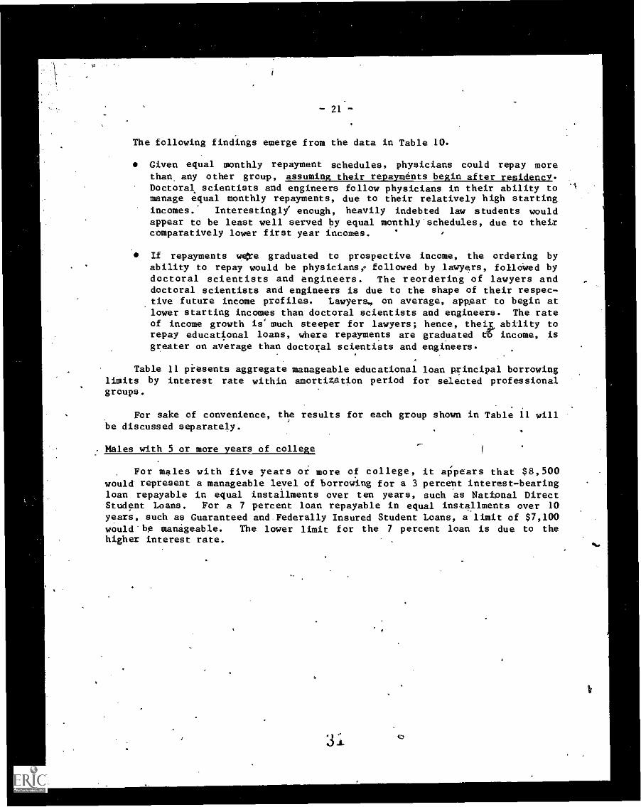
The following findings emerge from the data in Table 10.

Given equal monthly repayment schedules, physicians could repay morethan any other group, assuming their repayments begin after residency.Doctoral scientists and engineers follow physicians in their ability tomanage equal monthly repayments, due to their relatively high startingincomes. Interestingly' enough, heavily indebted law students wouldappear to be least well served by equal monthly'schedules, due to theircomparatively lower first year incomes.

If repayments were graduated to prospective income, the ordering byability to repay would be physicians, followed by lawyers, folloWed bydoctoral scientists and engineers. The reordering of lawyers anddoctoral scientists and engineers is due to the shape of their respec-tive future income profiles. Lawyers., on average, appear to begin atlower starting incomes than doctoral scientists and engineers. The rateof income growth is' much steeper for lawyers; hence, theix ability torepay educational loans, where repayments are graduated 6 income, is

greater on average than doctoral scientists and engineers.

Table 11 presents aggregate manageable educational loan principal borrowinglimits by interest rate within amortization period for selected professionalgroups.

For sake of convenience, the results for each group shown in Table 11 willbe discussed separately.

Males with 5 or more years of college

For males with five years or more of college, it appears that $8,500would represent a manageable level of borrowing for a 3 percent interest-bearingloan repayable in equal installments over ten years, such as National DirectStudent Loans. For a 7 percent loan repayable in equal installments over 10years, such as Guaranteed andFederally Insured Student Loans, a limit of $7,100would-be manageable. The lower limit for the 7 percent loan is due to thehigher interest rate.

-1

TABLE 11. Estimated Aggregate Manageable Educational Principal Borrowing Limits for Equal Installment and Graduated Rtpayment Option (GRO) Plansfor Selected Professional Groups (Amounts in Thousands) -s

.

Length of RepaymentPeriod/Interest Rate

Males with5 Yes or More of 'College

_.

- p

Lawyers

Physicians:Repayments

Beginning afterResidency

'Pysicians:i

Repayments Beginning0 Internship

Doctoral Scientistsend Engineers

Equal GraduatedRepay- RepaymentMents Option (GRO)

Equal GraduatedRepay- Repayment.meats Option (GRO)

Equal GraduatedRepay- Repayment °

merits Option (GRO)

Equal GraduatedRepay- Repaymentmente Option (GRO)

Equal GraduatedRepay- Repaymentmeats Option.(GRO)

10 Year Amortization

$ 8.5 $12.6-14.01

$ 7.1' $10.511.6

$ 6.2 $ 9.3-10.2

$11.9 $20.8-24.6

$ 9.1 $16.0-18.9

$ 7.6 $13.4-15.8

$14.8 $29.6-38.2

$10.5 $21.2-27.3

$ 8.5 $17.0-21.9

.

$ 7.7 $18.1-20.2

$ 6.4 $15.0-16.8

$ 5'.6 $13.2-14.7

$10.7. $33.5-40.8

$ 8.2 $25.7-31.4

$ 6.9 $21.5-26.3

.

$13.3 $53.2-71.9

$ 9.5 $38.1-51.4

$ 7.7 $30.6-41.3

$18.9 $33.7-38.1

$15.8 $28.1-31.8

$13.8 $24.6-27.9

.

$26.5 $62.3-77.8

$20.4 $47.9-59.8

$17.0 $40.1-50.0

.

$33.0 $100.9-140.4

$23.6 $72.2-100.5 '

$19.0 $60.0-80.7

.

$ 9.0 $16.5 -1B.4

$ 7.5 $13.7-15.3

$ 6.6 $12.0-13.5

.

$12.6. $32.5-39.9

$ 9.14_, $25.0-30.7

$ 8.1 .$20.9-25.7

Ate

$15.7 $55.6-76.4

$11.2 $39.7-54.7

$ 9.0 $31.9-43.9'

.

$11.2 $14.4-15.8

$ 9.3 $12.0-13.1

$ 8.2 $10.5-11.5

$15.6 : $22.8-26.9

$12.0 $17.5-20.6

$10.1 $14.6-17.3

$19.5 $32.4-41.4

$13:9 $23.1-29.6

$11.2, $18.4-23.8

____,

3% Interest

7% Interest

10% Interest

15 Year Amortization

3%.Interest

7% Interest

10% Interest

,..20 Year Amortization

3% Interest

7% Interest

10% Interest.

Assumed Year in whichRepayments Begin 1983 1982 1987

r

1983 1983

Estimated IncomeDuring First Yearof Repayment ,

$22.6 $21.0 $47.6 $23.5 $28.0

4

1Lower limit assume 3 percent annual. inflation rate;upper limit assumes 6 percent inflation rate.

-23-Or

These two findings suggest the advisability of (a) considering extensiOh,of the NDSL repayment period from 10 to.15 years for graduate and professionalstudents, if ;epayments are in equal installments, and (b) reviewing boti.thelength of the pay-back period and the equal installment norm f6r the Guaranteed-Student Loan Program.

If repayments were scaled to income, it appears that total borrowings-of$12,600 to $14,0001 iluld be manageable for graduate and professional studentsunder the National Direct Student Loan Program, given a 10-year repaymentperiod. Thus, one option would be to extend the NDSL loan maximum from $10,000

lito $15,000 and include a graduated repayment option fOr those whose debts exceed

18:,500.

These data also seem to suggest the advisability of considering revision ofthe Guaranteed Student Loan Program to permit postbaccalaureate students toborrow up to $16,000-$19,000, and to provide them the option of graduatedrepayments over 15 years if their debt exceeds $7,100.

4

Whether repayment periods should be extended to 20 years for graduate andprofessional students is debatable. Extension of the pay-back period to 20years could have the curious result of.expecting this generation of graduate andprofessional students to simultaneously repay their educational loans andcontribute toward their offspring's educational costs. It should be noted,hobever, that such an pxtension would significantly increase manageable loanprincipal limits.

Law Students

It was pointed out earlier that heavily indebted law students because oftheir relatively modest starting incomes, would appear to be least well served,particularly during the first repayment years, by equal installment loans.Their manageable aggregate loan principal for equal installment loans, whenrestricted to a proportion of the average first year salary, ranges from a lowof $5,600 for a 10 percent, 10 year loan, to $13,300 for a 3 percent, 20 yearloan: On the other hand, because of lawyers' typically more rapid-income growthexperience, graduating repayments to income would enable them to borrowconsiderably more, yet result in manageable annual repayments. For example, the

analysis in Table 11 suggests that law students'could comfortably borrow between$18,100 and $20,200, for a 10 year, 3 percent loan (such as NDSL),,providedrepayments were graduated to prospective income. From the perspective. oflawyers' income profiles, it appears as though the current Guaranteed StudentLoan aggregate borrowing limit of $15,000 is manageable at 7 percent interestand 10 years for pay-back, provided repayments are scaled to income. On theothSt hand, it appears that extension of the GSL pay-back petiod from 10 to 15years, and graduation of repayments to income, would increase the manageable GSLprincipal limits of law students to between $25,700 and $31,400.

Even at a 10 percent interest rate for a 15 year pay-back period, a indebt-edness of between $21,500 and $26,300 would not appear to be overly burdensomefor law students, on an income graduated basis.

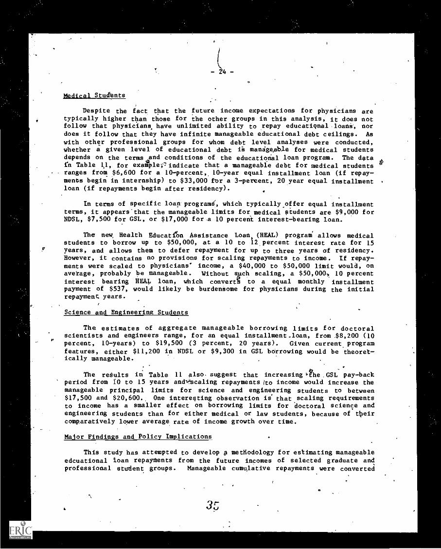
Medical Students

Despite the fact that the future income expectations for physicians aretypically higher than those for the other groups in this analysis, it does notfollow that physicians, have unlimited ability to repay educational loana, nordoes it follow that they have infinite manageable educational debt ceilings. As

with other professional groups for whom debt level analyses were conducted,whether a given level of educational debt ii manageable for medical studentsdepends on the termed conditions of the educational loan program. The data

$'fn Table 1,1, for example;',indicate that a manageable debt for medical studentsranges from $6,600 for a 10- percent, 10-year equal installment loan (if repay-ments begin in internship) to $33,000 for a 3-percent, 20 year equal installmentloan (if repayments begin after residency). 4

In terms of specific loan programa', which typically. offer equal installmentterms, it appears'that the manageable limits for medical students are $9,000 forNDSL, $7,500 for GSL, or $17,000 fora 10 percent interest-bearing loan.

The new Health EducatiOn Assistance Loan. (HEAL) programi allows medicalstudents to borrow up to $50,000, at a 10 to 12,percent interest rate for 15years, and allows them to defer repayment for up to three years of residency.However, it contains no provisions for scaling repayments to income. If repay-ments were scaled to physicians' income, a $40,000 to $50,000 limit would, onaverage, probably be manageable. Without shIch scaling, a $50,000., 10 percentinterest bearing HEAL loan, which converts to a equal monthly installmentpayment of $537, would likely be burdeniome for physicians during the initialrepayment years.

Science and Engineering Students

The estimates of aggregate manageable borrowing limits for doctoralscientists and engineers range, for an equal installment.loan, from 48,200 (10percent, 10-years) to $19,500 (3 percent, 20 years). Given current programfeatures, either $11,200 in NDSL or $9,300 in GSL borrowing would be theoret-ically manageable.

The results in Table 11 also. suggest that increasing ne.GSL pay-backperiod from 10 to 15 years and%?Iscaling repaymentsito income would increase themanageable principal limits for science and engineering students to between$17,500 and $20,600., One interesting observation is that scaling requirementsto income has a smaller effect on borrowing limits for doctoral science andengineering students than for either medical or law students, because of ttleircomparatively lower average rate of income growth over time.

Major Findings and Policy Implications

This study has attempted to develop p methodology for estimating manageableedcuational loan repayments from the future incomes of selected graduate andprofessional student groups. Manageable cumulative repayments were converted

3r

- 25 -

c-into aggregate loan princival limit's, given alternative intFiation periods and repaymentNlans (equal installment or gi(h,

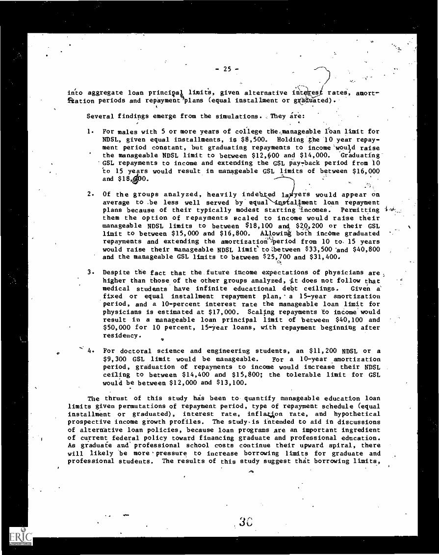
Several findings emerge from the simulations. , They ire:

resfffrates,, amortuated).'

1. For males with 5 or more years of college the4manageable loan limit forNDSL, given equal installments, is $8,500. Holding ',the '10 year repay-

ment period constant, but graduating repayments to income'wonld raisethe manageable NDSL limit to between $12,000 and $14,000. Graduatfng'GSL repayments to income and extending the GSL pay7back period from 10to 15 years would result in manageable GSL limits of between $16,000and $18,400.

2. Of the groups analyzed, heavily inde ed la yers would appear ohaverage to -be less well served by equal t= ailment loan repaymentplans because of their typically modest starting incomes. Permitting t

them the option of repayments scaled to income would raise theirmanageable NDSL limits to between $18,100 an $0,,200 or their GSLlimit to between $15,000 and $16,800. Allowink both income graduatedrepayments and extending the amortizatioieriod from 10 to 15 yearswould raise their manageable NDSL limit''tobetween $33,500 and $40,800and the manageable GSL limits to between $25,700 and $31,400.

3. Despite the fact that the future income expectations of physicians are;higher than those of the other groups analyzed, 4.t does not follow thatmedical students have infinite educational debt ceilings. Given afixed or equal installment repayment plan,' a 15-year amortizationperiod, and a 10-percent interest rate the manageable loan limit forphysicians is estimated at $17,000. Scaling repayments to income wouldresult in a manageable loan principal limit of between $40,100 and$50,000 for 10 percent, 15 -year loans, with repayment beginning afterresidency.

For doctoral science and engineering students, an $11,200 NDSL or a$9,300 GSL limit would be manageable. For a 10-year amortizationperiod, graduation of repayments to income would increase their NDSLceiling to between $14,400 and $15,800; the tolerable limit for GSLwould be between $12,000 and $13,100.

The thrust of this study his been to quantify manageable education loanlimits given permutations of repayment period, type of repayment schedule (equalinstallment or graduated), interest rate, infla4on rate, and hypotheticalprospective income giowth profiles. The study-is intended to aid in discussionsof alternative loan policies, because loan programs are an important ingredientof current federal policy toward financing graduate and professional education.As graduaES and' professional school costs continue their upward spiral, therewill likely 'be more pressure to increase borrowing limits for graduate andprofessional students. The results of this study suggest that borrowing limits,

-26-

repayment terms and amortization periods may require restructuring; otherwisegraduate and professional students could well fate an unmanageable repaymentlegacy. If loans are to play a key role in the future finahcing of graduate and'professional education, and if the Guaranteed or Federally Insured Program is tobe the federal student aid vehicle for this purpose, then it may be advisabletoconsider certain technical changes to the program:

(1) In order to maximize manageable debt loads of graduate and profes-sional students, their undergraduate educational indebtedness shouldbe minimized. This goal.can be achieved through expansion of ui1der-graduate grant programs such as the Basic Educational OpportunityGrant (BEOG) program and the Supplementary Education Opportunity Grant(SEOG) program.

(2) Giaduate and professional students whose educationil indebtedness,from all sources, exceeds an agreed-upon threshold amount, should beoffered Graduated Repayment Option- (GRO) plans, and the option of a15 year repayment period.

(3) Separate threshold limits, aggregate principal limits, and graduated'repayment schedules should be developed for. meaningful occupationalclusters and should be based on an assessment of their manageableeducational debt, - loads.

While loans are currently an importApt financing mechanism for graduate andprofession 1 students, they should t be viewed as a panadea either bystudents, licy analysts or financially stressed graduate and professionalschools. F llowehip programs and experiential work-study learning opportunitiesfor student in the arts, humanities, sciences, and professions are needed toinsure equ I access to graduate and professional school, as well as to fosterintellec 1 excellence.

V

.0;

4

4*

-277.

APPENDIX A

Formulas for Estimating

Manageable Educational Loan Repayments

Assuming First Repayment

. Begins in 1983

38

C

-.28-

elm

(1) Adjusted Income (AI) in year y

AI = S * (l +r)y -1 *Iy

Where: AI = Adjusted Income

S = Starting salary

r = inflation rate

y = specified year (i.e. first, second, third) of repaymentperiod

/ = Age-Income Ratio in year y

(2) Effective Income (EX) in year

EI = AI - FT - FICA - STY

Where; AIY

= Adjusted Income in year y of the amortization period

PTY

= Federal taxes in year y, based on 1977 tax schedules

FICA = Amount of social security taxes in year y computed asfollows:

FICA = 1293 x (1.05)Y-1

STy = State and other taxes in year y, computed as follows:

STy = AI x .08

39

":

tJ

47.xr =29-1

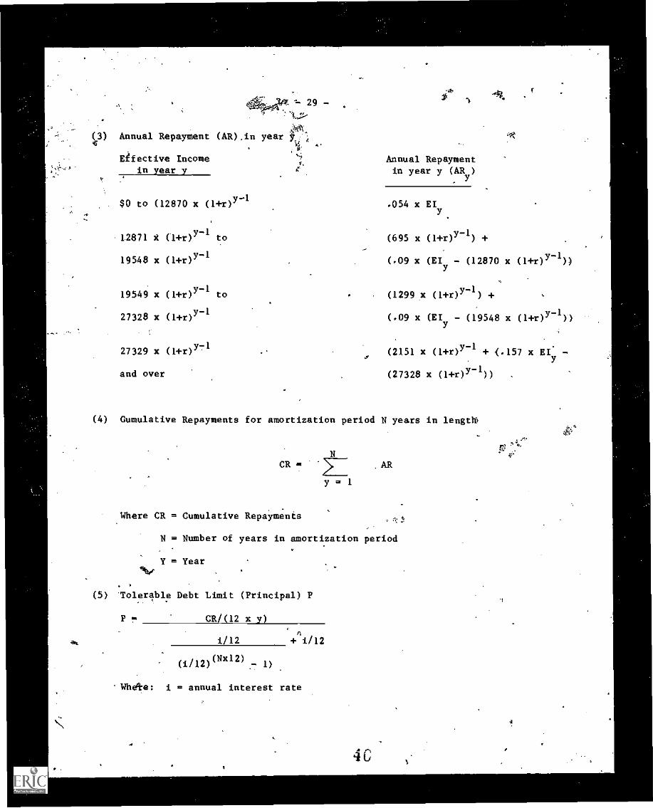
Ot,(43) Annual Repayment (AR) .in year

A!

Effective Incomein year y

. $0 to (12870 x (14T)Y-1

12871 t (+r)Y-I to

19548 x (1+0Y-I

19549 x (1+0Y-I to

27328 x (1+0Y-I

27329 x (1+0Y71

and over

Annual Repaymentin year y (AR y)

.054 x EIy

(695 x (1+0Y-1) +

(.09 x (EIy - (12870 x (140Y-1))

(1299.x (1+0Y-1) +

(.09 x (Ely - (19548 x (1+0Y-1))

(2151 x (1+0Y-I + <.157 x RI. -

(27328 x (1+0Y-1))

(4) Gumulative Repayments for amortization period N years in length

CR =

Y m 1

Where CR = Cumulative Repayments

N = Number of years in amortization period

Y = YearAv.

(5) 'Tolerable Debt Limit (Principal) P

P = CR/(12 x y)

aft i/12 + i/12

(i112)(NX12) 1)

Whete: i = annual interest rate

4C

-.31 -

1973 INCOME OP LAWYERS IN MASSACHUSETTS SURVEY

Years Admitted1

Mean 1Income

EstimatedAge

Less Than 1 .

\\ 1 - 4

\5 - 9

\10.7 14

15 -\19

20.- il\

$ 8,903

$15,135

$25,047

$31,585

$38,445

$42,173

24

25 - .28

29 - 33

34 - 38

39 - 43

44 - 53

Age. Mean AnnualMidpoint Growth Rate

J41

49

30%

10.5%

4 7%

4 0%

1 5%

1Source: Economic Survey Conducted by the Massachusetts Bar Association 197

4.

.MA4achusetts Bar Association, 1975, page 5.

Estimated Startirig Salary:

$11,000 in 1973 Dollarsx 1.81 Estimated Rise in CPI from 1973 - 1982,

(133.1 to 241.2).

$ 21.0 = Estimated Starting Salaryin 1982

-32i-

ESTIMATED MEAN 1973 INCOME OF LAWYERS BY AGE

Age*1973Income Ratio

25 $11.6 1.00

26 $15. 1 1.50

27 $16.6 1.43

28 $18.4 14 1.59

29 $20.3 1.75

30 $22.4 1.93

31 $25.0 2.16

32 $264 2.24

33 $27.2 2.34

34 $28.4 2.45

35 $29.8 2.57

36 $31.6 2.72

37 $32.4 2.79

38 $33.7 2.90

39 $35.1 3.03

40 $36.5 3.15

41 $37.9 3.27

42 $38.5 3.32

43 $39.1 3.37

44 $3947 3.42

45 $40.3 3.47

46 $40.9 3.53

47 $41.5 3.58

48 $42.1 3.63

49 $42.7 3.68

4 3

734-

PHYSICIANS MEAN PROFESSIONAL INCOMEIN 1977. DOLLARS

1977Age Income

26 16.7

27 17.7

28 '18.9

29 19.9

30 24.0

31 26.3

32 28.6

33 0.9

34

35 35.6

36 37.9

37 40.3

38 42.6

39 44.9

40 47.3

41 49.6

42 51.9

43 54.2

. 44 56.6

45 58.9

46 61.2

47 63.1

48 64.0

- 49 64.7

Ratio 1 Ratio 2

1.0

1.06

1.13

1.19

1.44 1..00

1.57 1.10

1.71 1.19

1.85 1.29

1.99 1.39

2.13 1.48

2.27 1.58

2.41 1.68

2.55 1.78

2.69 1.87

2.83 1.97

2.97 2.07

3.11 2.17

3.25 2.26

3.39 2.36

3.52 2.45

3.66 2.55

3.78 2.63

3.83 2.76

3.87 2.70

Source: Unpublished Data, Institute of Demographic and EconoMic Studies

Ratio 1 - Assumes repayments start during internship

Ratio 2 - Assumds deferment during one year of residency and three yearsof internship.

I

.7

-35-

J

ESTIMATED STARTING INCOME OF PHYSICIANS

In 1983, at age 26

816,700 26 year old's income in 1977 dollars

x 1.407 Rise in CPI from 1977 to 1983(181.6 to ,255.5)

$23,496 =, Estimated mean 1983 income of 26 year old.

In 1987, a

$24,000 ... 30 year old's income in 1977 dollars

x 1.776 Estimated' rise in CPI from 1977 to 1987

. (181.6 to 322.6)

$42,624 = Estimated mean income of 30 year oldin 1987 dollars.

I

46

Income of Doctoral Scientists and Engineers

- 37 -

ESTIMATED MEDIAN 1983 STARTING INCOME OFDOCTORAL SCIENTISTS AND ENGINEERS

Estimated Income of 26 year oldin 1973 dollars $14,600

Rise in CPI from1973 to 198:3(133.1 to 255.5) 1 92

Estimated 1983 starting income = $28,032

IC

Ot

-38-

UNITED STATES DOCTORAL SCIENTISTS AND ENGINEERS

Median Annual Salary by Age -- 1973

Under 30

30-34

35-39

40-44

45-49

50-54

55-59

60-64

Over 64

"MeanAnnual

dian 1973 Age Growtha'lary 1 Midpoint Rate

$15,500 . 28

17,500 32

19,660 37

22,000 42

A 24,200 47

25,000 52

25,300 57

25,800 62

24,700

..... 1.032

1 023

1 022

1 018

1 0065

1 0024

1 004

1Source: Doctoial Scientists and Engineers in the United States:

1973 Profile, National Academy of Sciences, March 1974,page 25, Table 10. ,

I

-39-

INTERPOLATED MEDIAN 1973 SALARY OFDOCTORAL SCIENTISTS AND ENGINEERS

Age 0+.1973

Salary Ratio

26 14.6

27 14.9

28 15.5

29 16.0

30 16.5

31 17.0

32 17.5

33 17.9

34 18.3

35 18.7

r9.2

37 19.6

38 20.1

39 A 20.5

40 21.0

41 21.5,

42 22.0

43 22.4

44 22.8

45 23.3

1.00

1.02

1.06

1.10

1.13

1.16

1.20

,1.22

1.25

1.28

1.32

1.34

1.38

1.41

1.44

1.47

1.51

1.53

1:56

1.60

So