Estimating Platform Market Power in Two-Sided Markets withan Application to Magazine Advertising

Minjae Song∗

July 2011†

Abstract

In this paper I estimate platform markups in two-sided markets using structural models ofplatform demand. My models and estimation procedure are applicable to general two-sidedmarket settings where agents on each side care about the presence of agents on the other sideand platforms set two membership prices to maximize the sum of profits. Using data on TVmagazines in Germany I show that the magazines typically set copy prices below marginalcosts and earn profits from selling advertising pages. I also show that mergers are much lessanticompetitive than in one-sided markets and could even be welfare enhancing.

Keywords: Platform competition, two-sided single-homing, competitive bottleneck, mergersimulation

∗Simon Graduate School of Business, Box 270100, University of Rochester, Rochester, NY 14627-0100. E-mail:minjae.song@simon.rochester.edu. I have benefited from discussions with Paul Ellickson, Marshall Freimer, DanielHalbheer, Ulrich Kaiser, Jeanine Miklos-Thal, Sanjog Misra, Michael Raith, Kyoungwon Seo, and participants atvarious conferences and seminars. I especially thank Ulrich Kaiser for providing me with the data used in this paper.All errors are mine.†First version: September 2009.

1

1 Introduction

Two-sided markets are characterized by two groups of agents interacting through intermediaries

or platforms. Agents in each group care about the presence of the other group, creating cross-

group externalities, and their economic decisions, such as which platform to join, affect the utility

of the other group’s agents. Platforms account for these externalities in their strategic decisions

such as setting prices. Examples are numerous, including the payment system where merchants

and consumers interact through credit cards, video game systems where game developers and

consumers interact through video consoles, print media where advertisers and readers interact

through newspapers or magazines, etc. Rysman (2009) provides more examples and an overview

on the literature.

In this paper I use structural models of platform demand to estimate platform markups

in two-sided markets. Because of the cross-group externalities, prices in two-sided markets can

be either higher or lower than profit maximizing prices in one-sided markets. This means that,

without considering the two sides simultaneously, researchers will obtain incorrect markups even

with consistent demand estimates. The two-sidedness also complicates merger evaluations as higher

market power does not necessarily result in higher post-merger prices on either side of the market.

One of challenges in the markup estimation in two-sided markets is tracing a feedback loop

that a price perturbation triggers. Suppose two groups, say group A and group B, appreciate the

presence of the other group on platforms. When a platform attracts more of group A agents, say

because of lowered prices or due to a demand shock, it becomes more attractive to group B agents

and attracts more of them. This will make the platform more attractive to group A agents, which,

in turn, attracts more group B agents, and so on.

In order to fully trace the feedback loop, I treat a demand system as a system of implicit

functions. In this system agents of each side decide which platform to join, given prices, the size of

agents from the other side, and other platform attributes. Given this demand system, platforms set

two prices to maximize joint profits from both sides. The price elasticity, which is the key component

2

in markup estimations, can be numerically computed using properties of implicit functions.

I consider both a two-sided single-homing model and a competitive bottleneck model. In

the single-homing model, agents of both groups join only one platform (single-home). In the

competitive bottleneck model, one set of agents joins as many platforms as they like (multi-home)

while the other set single-homes. Night clubs are an example of the former, where men and women

choose one club. Magazine advertising is an example of the latter, where advertisers advertise in

multiple magazines while readers choose one magazine in each segment.1 In both models I focus

on a case where platforms only charge fixed fees for membership.

Numerical simulations show that equilibrium outcomes in the considered models are drasti-

cally different from those of the one-sided market. When the cross-group externalities are substan-

tial, platforms may charge below-cost prices to agents on one side to make profit on the other side.

Even when prices are above costs, they are not necessarily set on the elastic part of the demand

curve. The feedback loop is quantitatively significant such that the price elasticity, when computed

without fully tracing it, can be different by more than fifty percent.

For demand estimation I use the generalized method of moments, which is in the same spirit

of an estimation procedure widely used in the industrial organization literature (Berry 1994; Berry,

Levinsohn, and Pakes, 1995; and many others). Given data on platform prices, market shares

and attributes, the agents’mean utilities from each platform are recovered by equating model-

predicted market shares to the observed ones. These mean utilities are assumed to be a linear

function of platforms’ attributes. Model parameters are estimated by using moment conditions

that instrumental variables are not correlated with unobserved platform attributes or demand

shocks. There are two important differences from the standard demand estimation. First, there

are two demand equations to estimate, one for each side. Second, the size of agents on the other

side is included as a platform attribute and this variable is an endogenous variable in addition to

the price variable.

1However, many real world cases have both features. Consider heterosexual dating agencies, another example ofthe single-homing setting. In the real world men and women may choose multiple dating agencies at the same time.

3

As an empirical application I use data on TV magazines in Germany and estimate the

competitive bottleneck model where advertisers advertise in as many magazines as they want. Two

membership fees are the copy price charged to readers and the per-page advertising price charged

to advertisers. The number of copies sold and the number of advertising pages are proxies for the

number of readers and advertisers joining magazines. The average copy price is about one euro,

while the average advertising price per page is close to 30,000 euros. The magazine on average sells

about 1.5 million copies in a quarter and has about 250 advertising pages, which means that the

advertising revenue is five times as large as the sales revenue.

My results show that magazines typically do not make any profit from selling copies. More

than eighty percent of magazines set copy prices below marginal costs, while earning a huge markup,

about seventy percent on average, from advertising. Combining the two sides, the joint profit is

about 1 million euros on average per quarter. When the advertising side is ignored, the same

demand estimates imply seventy percent average markup on the reader side with forty percent of

magazines facing inelastic demand.

Taking the advantage of having structural models for both sides, I calculate equilibrium

outcomes for hypothetical ownership structures.2 Results show that when the market becomes

more concentrated, copy prices do not necessarily increase as magazines try to attract more readers.

Results also show that larger reader bases resulting from lower copy prices may increase advertisers’

demand so much that magazines charge higher advertising prices and attract still more advertisers.

This implies that even when a merger increases a publisher’s market power on both sides of the

market, readers may be better off, or at least less worse off, than predicted by one-sided market

models.

There are numerous papers that theoretically analyze various issues related to two-sided

markets, of which Rochet and Tirole (2006) provide a thorough review. Among them, my structural

models are closely related to the canonical models in Armstrong (2006) but I extend them to a more

2Finding equilibrium prices is computationally more intensive than for one-sided markets as it requires finding aset of market shares that simultaneously satisfies the demand system for each trial value.

4

general oligopolistic setting. While Armstrong confines a demand function to Hotelling’s framework,

I adopt a more general discrete choice framework for consumers’single-homing decisions. Thus, in

my models platforms are differentiated products with the presence of the other-side agents as an

endogenous attribute.

My models, however, are not applicable to markets where platforms charge usage or per-

transaction fees as, for example, in the credit card industry. Rochet and Tirole (2003) develop a

model where platforms charge usage fees and Rochet and Tirole (2006) extend it to integrate usage

and membership fees in a monopoly platform setting. Although a two-part tariff structure (a fixed

membership fee plus a usage fee proportional to the size of the other-side members) is often seen

in many industries, it is beyond the scope of my paper.3

Empirical research on the two-sided market is relatively scarce but steadily growing. Distin-

guished from existing empirical studies, my paper brings in two important features of the two-sided

market together. The first feature is that agents of each side care about the presence of agents on

the other side. This feature is the main factor driving the feedback loop but is suppressed in some

studies by assuming that one of the two groups does not care about the presence of the other. For

example, Argentesi and Filistrucchi (2007) , in studying the Italian newspaper market, assume that

readers are indifferent about advertising in newspapers. Although this assumption makes a model

more tractable, it misses the essence of the two-sidedness.

The second feature is that platforms set two prices, one for each side. Free membership

(or zero price) granted to one group of agents, observed in some of two-sided markets such as the

radio industry and the online search engine industry, is part of the platforms’profit maximization

behaviors. However, this zero price is often taken as an exogenous constraint in modeling platform

behaviors. Examples include Rysman (2004) on the Yellow Pages and Jeziorski (2011) on the

radio industry. As far as I know, Kaiser and Wright (2006) is the only structural empirical paper

3A well-known proposition in Armstrong (2006) shows that a continuum of equilibria exists when platformscompete in the two-part tariff. Weyl and White (2010) propose a new equilibrium concept to circumvent thisproblem.

5

that has both features together, but their model is only applicable to a duopoly in the symmetric

equilibrium.

There are also empirical studies that test predictions from theoretical models using reduced-

form regressions. For example, Jin and Rysman (2010) use data from baseball card conventions

and test whether the conventions’pricing behaviors are consistent with the single-homing model in

Armstrong (2006) . Chandra and Collard-Wexler (forthcoming) develop a two-sided market model

in the Hotelling framework, derive predictions on post-merger price changes, and test them using

data from the Canadian newspaper market.

The paper is organized as follows: Section 2 presents two models of the two-sided market,

followed by an estimation procedure in section 3. Section 4 presents simulation results and section

5 presents empirical results. Section 6 concludes.

2 Models

2.1 Two-Sided Single-Homing Model

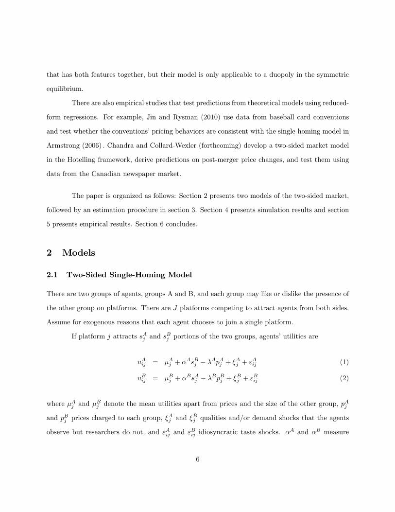
There are two groups of agents, groups A and B, and each group may like or dislike the presence of

the other group on platforms. There are J platforms competing to attract agents from both sides.

Assume for exogenous reasons that each agent chooses to join a single platform.

If platform j attracts sAj and sBj portions of the two groups, agents’utilities are

uAij = µAj + αAsBj − λApAj + ξAj + εAij (1)

uBij = µBj + αBsAj − λBpBj + ξBj + εBij (2)

where µAj and µBj denote the mean utilities apart from prices and the size of the other group, pAj

and pBj prices charged to each group, ξAj and ξ

Bj qualities and/or demand shocks that the agents

observe but researchers do not, and εAij and εBij idiosyncratic taste shocks. α

A and αB measure

6

the (dis)utility of interacting with agents of the other group and λA and λB the disutility of price.

Consumers may choose the outside option of joining no platform and receive zero mean utility and

an idiosyncratic shock.

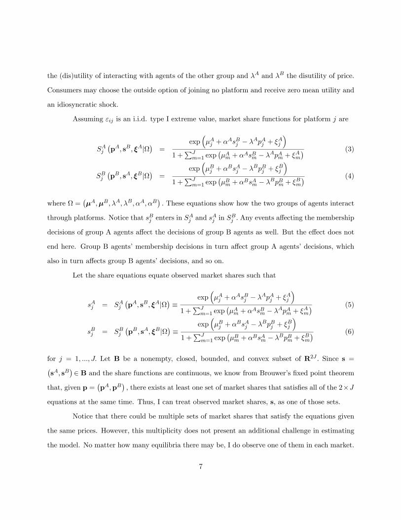
Assuming εij is an i.i.d. type I extreme value, market share functions for platform j are

SAj(pA, sB, ξA|Ω

)=

exp(µAj + αAsBj − λApAj + ξAj

)1 +

∑Jm=1 exp

(µAm + αAsBm − λApAm + ξAm

) (3)

SBj(pB, sA, ξB|Ω

)=

exp(µBj + αBsAj − λBpBj + ξBj

)1 +

∑Jm=1 exp

(µBm + αBsAm − λBpBm + ξBm

) (4)

where Ω =(µA,µB, λA, λB, αA, αB

). These equations show how the two groups of agents interact

through platforms. Notice that sBj enters in SAj and s

Aj in S

Bj . Any events affecting the membership

decisions of group A agents affect the decisions of group B agents as well. But the effect does not

end here. Group B agents’membership decisions in turn affect group A agents’decisions, which

also in turn affects group B agents’decisions, and so on.

Let the share equations equate observed market shares such that

sAj = SAj(pA, sB, ξA|Ω

)≡

exp(µAj + αAsBj − λApAj + ξAj

)1 +

∑Jm=1 exp

(µAm + αAsBm − λApAm + ξAm

) (5)

sBj = SBj(pB, sA, ξB|Ω

)≡

exp(µBj + αBsAj − λBpBj + ξBj

)1 +

∑Jm=1 exp

(µBm + αBsAm − λBpBm + ξBm

) (6)

for j = 1, ..., J. Let B be a nonempty, closed, bounded, and convex subset of R2J . Since s =(sA, sB

)∈ B and the share functions are continuous, we know from Brouwer’s fixed point theorem

that, given p =(pA,pB

), there exists at least one set of market shares that satisfies all of the 2×J

equations at the same time. Thus, I can treat observed market shares, s, as one of those sets.

Notice that there could be multiple sets of market shares that satisfy the equations given

the same prices. However, this multiplicity does not present an additional challenge in estimating

the model. No matter how many equilibria there may be, I do observe one of them in each market.

7

Given this observation, all I need for identification is instrumental variables that are not correlated

with demand shocks but correlated with the other side’s market shares. This even means that I do

not need to use both sides to consistently estimate demand for one side.4

It is worth comparing multiplicity in the two-sided market model with multiplicity in

the empirical game literature where multiple equilibria make model estimation more challenging.

Consider a static incomplete information entry game with two firms. Firm 1’s probability of entry

is a function of firm 2’s probability of entry, and vice versa, and these probability functions look

similar to equations (5) and (6) with the type I extreme value distribution assumption on the

idiosyncratic shock. The key difference is that researchers do not observe the entry probability and

should compute it as a solution to the game. However, it is not guaranteed that they obtain the

same equilibrium in all markets.

2.2 Competitive Bottleneck Model

In the competitive bottleneck model, while one group, group A, deals with a single platform (single-

homes), the other group, group B, deals with multiple platforms (multi-homes). This is a situation

where group B puts more weight on the network-benefits of being in contact with the widest

population of group A consumers than it does on the costs of dealing with more than one platform.

An example often used for this model is media advertising. Group A agents are readers who care

about media content and may or may not like advertising. The other group agents are advertisers

who want to reach as many readers as possible.

Following Armstrong (2006) I assume that a group B agent makes a decision to join one

platform independently from its decision to join another as long as its net benefit is positive. In

this sense there is no direct competition between platforms to attract group B agents and each

platform acts as a monopolist towards them. For group A agents I use the same utility function

used in the single-homing model except that I use the number of group B agents instead of their

4However, multiple equilibria comes into play in counterfactual exercises.

8

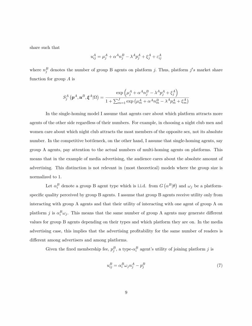
share such that

uAij = µAj + αAnBj − λApAj + ξAj + εAij

where nBj denotes the number of group B agents on platform j. Thus, platform j′s market share

function for group A is

SAj(pA,nB, ξA|Ω

)=

exp(µAj + αAnBj − λApAj + ξAj

)1 +

∑Jm=1 exp

(µAm + αAnBm − λApAm + ξAm

)In the single-homing model I assume that agents care about which platform attracts more

agents of the other side regardless of their numbers. For example, in choosing a night club men and

women care about which night club attracts the most members of the opposite sex, not its absolute

number. In the competitive bottleneck, on the other hand, I assume that single-homing agents, say

group A agents, pay attention to the actual numbers of multi-homing agents on platforms. This

means that in the example of media advertising, the audience cares about the absolute amount of

advertising. This distinction is not relevant in (most theoretical) models where the group size is

normalized to 1.

Let αBi denote a group B agent type which is i.i.d. from G(αB|θ

)and ωj be a platform-

specific quality perceived by group B agents. I assume that group B agents receive utility only from

interacting with group A agents and that their utility of interacting with one agent of group A on

platform j is αBi ωj . This means that the same number of group A agents may generate different

values for group B agents depending on their types and which platform they are on. In the media

advertising case, this implies that the advertising profitability for the same number of readers is

different among advertisers and among platforms.

Given the fixed membership fee, pBj , a type-αBi agent’s utility of joining platform j is

uBij = αBi ωjnAj − pBj (7)

9

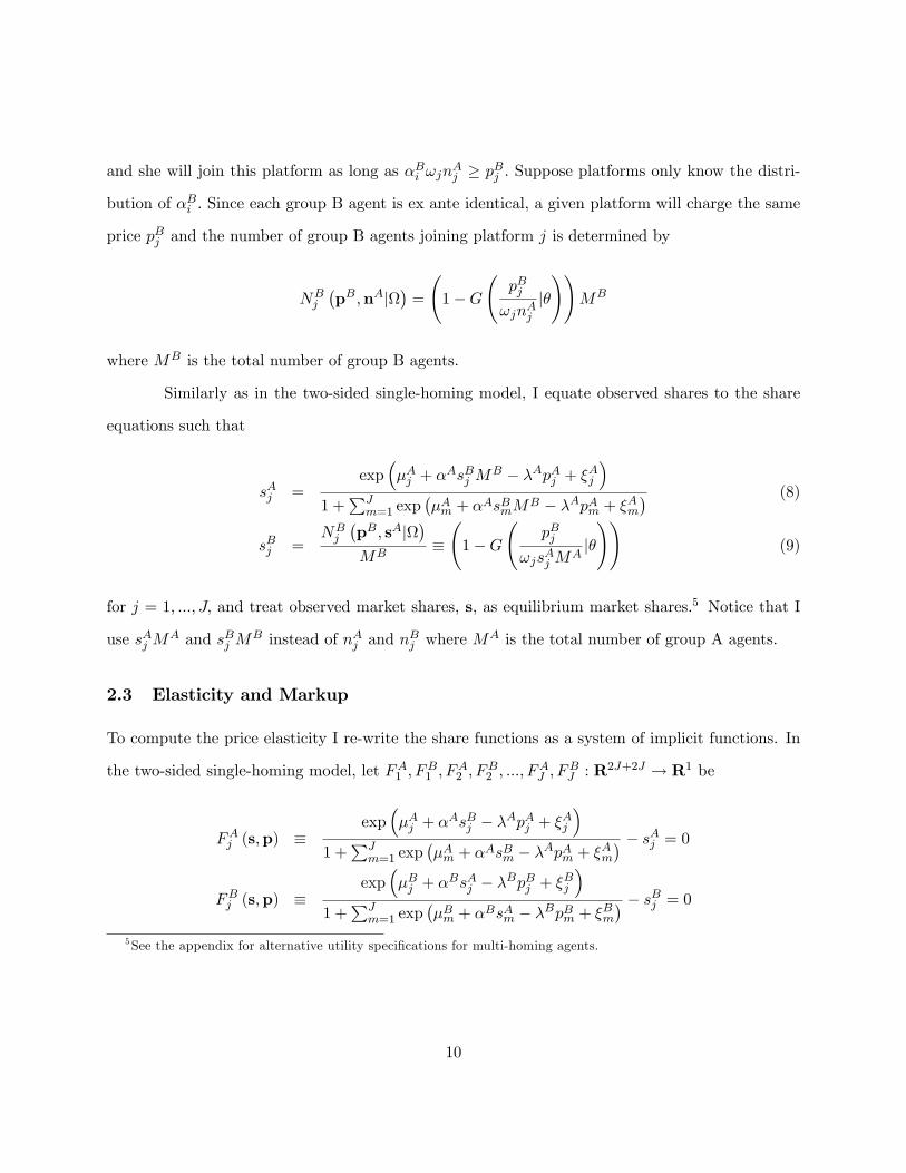
and she will join this platform as long as αBi ωjnAj ≥ pBj . Suppose platforms only know the distri-

bution of αBi . Since each group B agent is ex ante identical, a given platform will charge the same

price pBj and the number of group B agents joining platform j is determined by

NBj

(pB,nA|Ω

)=

(1−G

(pBj

ωjnAj|θ))

MB

where MB is the total number of group B agents.

Similarly as in the two-sided single-homing model, I equate observed shares to the share

equations such that

sAj =exp

(µAj + αAsBj M

B − λApAj + ξAj

)1 +

∑Jm=1 exp

(µAm + αAsBmM

B − λApAm + ξAm) (8)

sBj =NBj

(pB, sA|Ω

)MB

≡(

1−G(

pBj

ωjsAj MA|θ))

(9)

for j = 1, ..., J, and treat observed market shares, s, as equilibrium market shares.5 Notice that I

use sAj MA and sBj M

B instead of nAj and nBj where M

A is the total number of group A agents.

2.3 Elasticity and Markup

To compute the price elasticity I re-write the share functions as a system of implicit functions. In

the two-sided single-homing model, let FA1 , FB1 , F

A2 , F

B2 , ..., F

AJ , F

BJ : R2J+2J → R1 be

FAj (s,p) ≡exp

(µAj + αAsBj − λApAj + ξAj

)1 +

∑Jm=1 exp

(µAm + αAsBm − λApAm + ξAm

) − sAj = 0

FBj (s,p) ≡exp

(µBj + αBsAj − λBpBj + ξBj

)1 +

∑Jm=1 exp

(µBm + αBsAm − λBpBm + ξBm

) − sBj = 0

5See the appendix for alternative utility specifications for multi-homing agents.

10

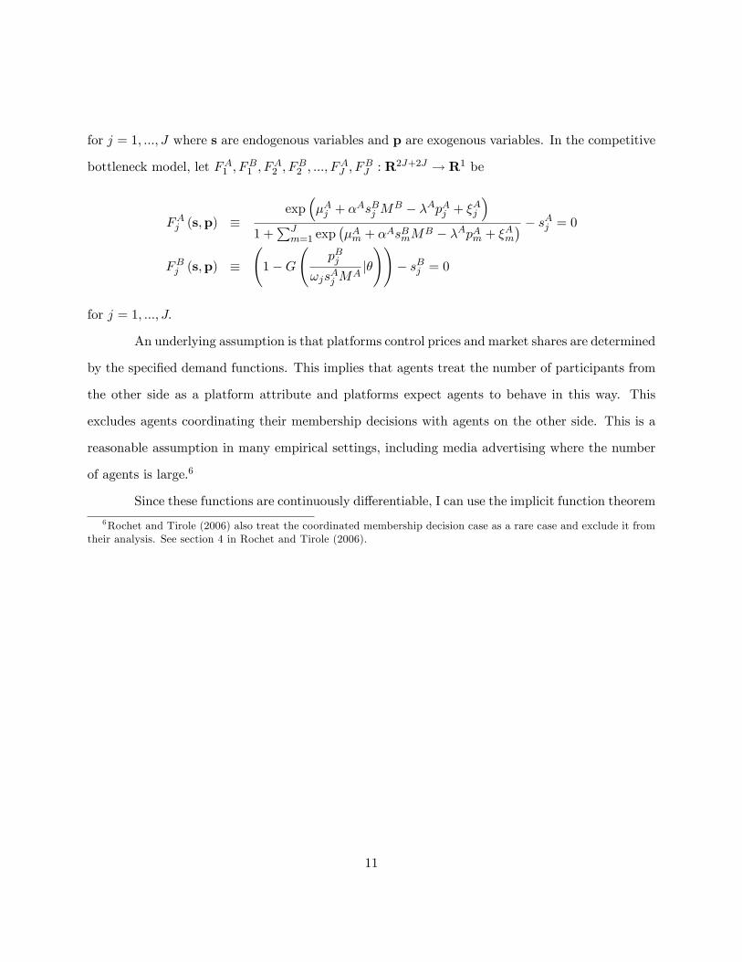
for j = 1, ..., J where s are endogenous variables and p are exogenous variables. In the competitive

bottleneck model, let FA1 , FB1 , F

A2 , F

B2 , ..., F

AJ , F

BJ : R2J+2J → R1 be

FAj (s,p) ≡exp

(µAj + αAsBj M

B − λApAj + ξAj

)1 +

∑Jm=1 exp

(µAm + αAsBmM

B − λApAm + ξAm) − sAj = 0

FBj (s,p) ≡(

1−G(

pBj

ωjsAj MA|θ))− sBj = 0

for j = 1, ..., J.

An underlying assumption is that platforms control prices and market shares are determined

by the specified demand functions. This implies that agents treat the number of participants from

the other side as a platform attribute and platforms expect agents to behave in this way. This

excludes agents coordinating their membership decisions with agents on the other side. This is a

reasonable assumption in many empirical settings, including media advertising where the number

of agents is large.6

Since these functions are continuously differentiable, I can use the implicit function theorem

6Rochet and Tirole (2006) also treat the coordinated membership decision case as a rare case and exclude it fromtheir analysis. See section 4 in Rochet and Tirole (2006).

11

to compute the price elasticity. For a price change by platform j

∂sA1 /∂pAj ∂sA1 /∂p

Bj

∂sB1 /∂pAj ∂sB1 /∂p

Bj

......

∂sAJ /∂pAj ∂sAJ /∂p

Bj

∂sBJ /∂pAj ∂sBJ /∂p

Bj

= −

∂FA1 /∂sA1 ∂FA1 /∂s

B1 · · · ∂FA1 /∂s

AJ ∂FA1 /∂s

BJ

∂FB1 /∂sA1 ∂FB1 /∂s

B1 · · · ∂FB1 /∂s

AJ ∂FB1 /∂s

BJ

......

. . ....

...

∂FAJ /∂sA1 ∂FAJ /∂s

B1 · · · ∂FAJ /∂s

AJ ∂FAJ /∂s

BJ

∂FBJ /∂sA1 ∂FBJ /∂s

B1 · · · ∂FBJ /∂s

AJ ∂FBJ /∂s

BJ

−1

×

∂FA1 /∂pAj ∂FA1 /∂p

Bj

∂FB1 /∂pAj ∂FB1 /∂p

Bj

......

∂FAJ /∂pAj ∂FAJ /∂p

Bj

∂FBJ /∂pAj ∂FBJ /∂p

Bj

, (10)

provided that the inverse matrix is non-singular.7

Suppose there are two platforms. For platform 1’s price change in the two-sided single-

homing model,

∂FA1 /∂sA1 ∂FA1 /∂s

B1 ∂FA1 /∂s

A2 ∂FA1 /∂s

B2

∂FB1 /∂sA1 ∂FB1 /∂s

B1 ∂FB1 /∂s

A2 ∂FB1 /∂s

B2

∂FA2 /∂sA1 ∂FA2 /∂s

B1 ∂FA2 /∂s

A2 ∂FA2 /∂s

B2

∂FB2 /∂sA1 ∂FB2 /∂s

B1 ∂FB2 /∂s

A2 ∂FB2 /∂s

B2

−1

=

−1 αAsA1(1− sA1

)0 −αAsA1 sA2

αBsB1(1− sB1

)−1 −αBsB1 sB2 0

0 −αAsA1 sA2 −1 αAsA2(1− sA2

)−αBsB1 sB2 0 αBsB2

(1− sB2

)−1

−1

7Note that this is still a valid formula when platforms are constrained to grant free access to one side of the market.

12

and

∂FA1 /∂pA1 ∂FA1 /∂p

B1

∂FB1 /∂pA1 ∂FB1 /∂p

B1

∂FA2 /∂pA1 ∂FA2 /∂p

B1

∂FB2 /∂pA1 ∂FB2 /∂p

B1

=

−λAsA1(1− sA1

)0

0 −λBsB1(1− sB1

)λAsA1 s

A2 0

0 λBsB1 sB2

In the competitive bottleneck model,

∂FA1 /∂sA1 ∂FA1 /∂s

B1 ∂FA1 /∂s

A2 ∂FA1 /∂s

B2

∂FB1 /∂sA1 ∂FB1 /∂s

B1 ∂FB1 /∂s

A2 ∂FB1 /∂s

B2

∂FA2 /∂sA1 ∂FA2 /∂s

B1 ∂FA2 /∂s

A2 ∂FA2 /∂s

B2

∂FB2 /∂sA1 ∂FB2 /∂s

B1 ∂FB2 /∂s

A2 ∂FB2 /∂s

B2

−1

=

−1 αAMBsA1(1− sA1

)0 −αAMBsA1 s

A2

pB1

ω1MA(sA1 )2 g(

pB1ω1sA1MA

|θ)

−1 0 0

0 −αAMBsA1 sA2 −1 αAMBsA2

(1− sA2

)0 0

pB2

ω2MA(sA2 )2 g(

pB2ω2sA2MA

|θ)

−1

−1

and

∂FA1 /∂pA1 ∂FA1 /∂p

B1

∂FB1 /∂pA1 ∂FB1 /∂p

B1

∂FA2 /∂pA1 ∂FA2 /∂p

B1

∂FB2 /∂pA1 ∂FB2 /∂p

B1

=

−λAsA1(1− sA1

)0

0 −1ω1sA1M

A g(

pB1ω1sA1M

A |θ)

λAsA1 sA2 0

0 0

where g (.) is the pdf of the group B agent’s type distribution.

Notice that, were it not for the two-sidedness, the second term in (10) multiplied by the

price-share ratio would be the price elasticity and that all cross-group terms, (∂FAk /∂pBj and

∂FBk /∂pAj , for k = 1, ..., J) would be zero. Moreover, in the competitive bottleneck model the

cross-price elasticity on the agent B side (∂FBr /∂pBj , r 6= j) would also be zero. Notice also that

the literature usually approximates price elasticity by considering only the direct impact of a price

13

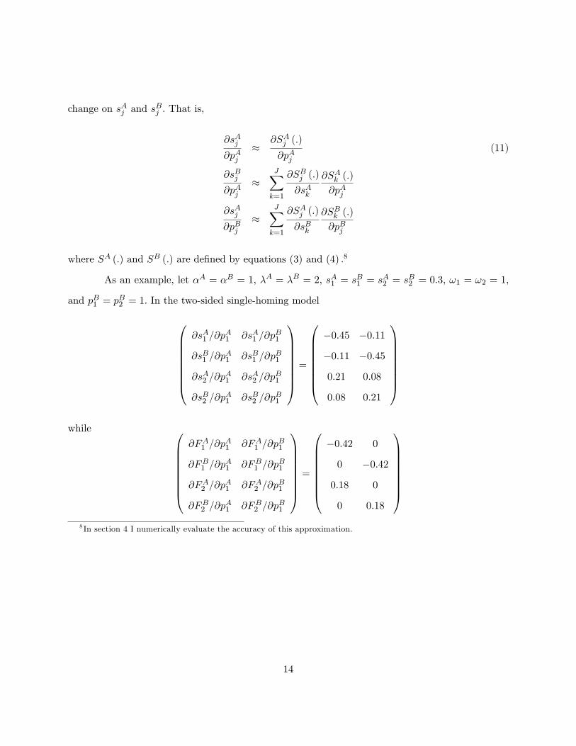
change on sAj and sBj . That is,

∂sAj

∂pAj≈

∂SAj (.)

∂pAj(11)

∂sBj

∂pAj≈

J∑k=1

∂SBj (.)

∂sAk

∂SAk (.)

∂pAj

∂sAj

∂pBj≈

J∑k=1

∂SAj (.)

∂sBk

∂SBk (.)

∂pBj

where SA (.) and SB (.) are defined by equations (3) and (4) .8

As an example, let αA = αB = 1, λA = λB = 2, sA1 = sB1 = sA2 = sB2 = 0.3, ω1 = ω2 = 1,

and pB1 = pB2 = 1. In the two-sided single-homing model

∂sA1 /∂pA1 ∂sA1 /∂p

B1

∂sB1 /∂pA1 ∂sB1 /∂p

B1

∂sA2 /∂pA1 ∂sA2 /∂p

B1

∂sB2 /∂pA1 ∂sB2 /∂p

B1

=

−0.45 −0.11

−0.11 −0.45

0.21 0.08

0.08 0.21

while

∂FA1 /∂pA1 ∂FA1 /∂p

B1

∂FB1 /∂pA1 ∂FB1 /∂p

B1

∂FA2 /∂pA1 ∂FA2 /∂p

B1

∂FB2 /∂pA1 ∂FB2 /∂p

B1

=

−0.42 0

0 −0.42

0.18 0

0 0.18

8 In section 4 I numerically evaluate the accuracy of this approximation.

14

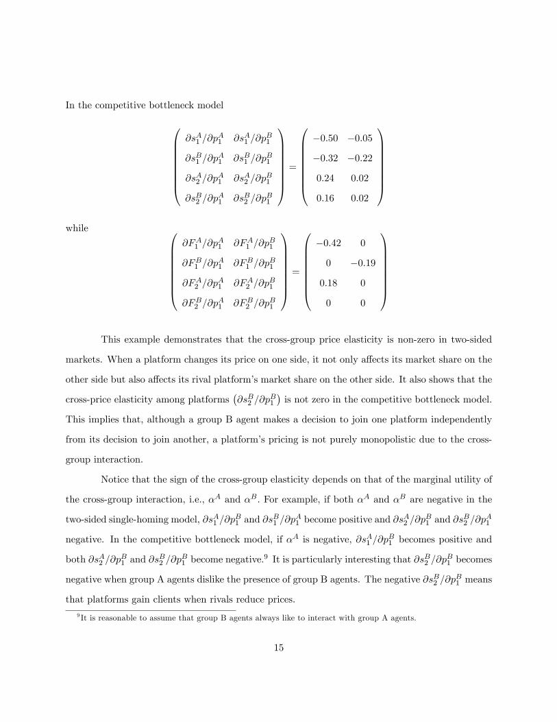
In the competitive bottleneck model

∂sA1 /∂pA1 ∂sA1 /∂p

B1

∂sB1 /∂pA1 ∂sB1 /∂p

B1

∂sA2 /∂pA1 ∂sA2 /∂p

B1

∂sB2 /∂pA1 ∂sB2 /∂p

B1

=

−0.50 −0.05

−0.32 −0.22

0.24 0.02

0.16 0.02

while

∂FA1 /∂pA1 ∂FA1 /∂p

B1

∂FB1 /∂pA1 ∂FB1 /∂p

B1

∂FA2 /∂pA1 ∂FA2 /∂p

B1

∂FB2 /∂pA1 ∂FB2 /∂p

B1

=

−0.42 0

0 −0.19

0.18 0

0 0

This example demonstrates that the cross-group price elasticity is non-zero in two-sided

markets. When a platform changes its price on one side, it not only affects its market share on the

other side but also affects its rival platform’s market share on the other side. It also shows that the

cross-price elasticity among platforms(∂sB2 /∂p

B1

)is not zero in the competitive bottleneck model.

This implies that, although a group B agent makes a decision to join one platform independently

from its decision to join another, a platform’s pricing is not purely monopolistic due to the cross-

group interaction.

Notice that the sign of the cross-group elasticity depends on that of the marginal utility of

the cross-group interaction, i.e., αA and αB. For example, if both αA and αB are negative in the

two-sided single-homing model, ∂sA1 /∂pB1 and ∂s

B1 /∂p

A1 become positive and ∂s

A2 /∂p

B1 and ∂s

B2 /∂p

A1

negative. In the competitive bottleneck model, if αA is negative, ∂sA1 /∂pB1 becomes positive and

both ∂sA2 /∂pB1 and ∂s

B2 /∂p

B1 become negative.

9 It is particularly interesting that ∂sB2 /∂pB1 becomes

negative when group A agents dislike the presence of group B agents. The negative ∂sB2 /∂pB1 means

that platforms gain clients when rivals reduce prices.

9 It is reasonable to assume that group B agents always like to interact with group A agents.

15

I use demand estimates and the profit maximization conditions to recover platforms’oper-

ating costs. Platform j maximizes its profit by setting membership prices for the two groups, pAj

and pBj . Assuming the constant marginal cost, platform j’s profit is

πj =(pAj − cAj

)sAj M

A +(pBj − cBj

)sBj M

B

where MA and MB denote the total number of agents for each group respectively. The profit

maximizing first order conditions are

∂πj

∂pAj= sAj M

A +(pAj − cAj

) ∂sAj∂pAj

MA +(pBj − cBj

) ∂sBj∂pAj

MB = 0 (12)

∂πj

∂pBj= sBj M

B +(pBj − cBj

) ∂sBj∂pBj

MB +(pAj − cAj

) ∂sAj∂pBj

MA = 0 (13)

where all the share derivatives are computed by (10). The two marginal costs should be searched

simultaneously such that the two conditions are satisfied at the same time for each platform.10

Re-arranging equations (12) and (13) gives

(pAj − cAj

)= −pAj

(∂sAj

∂pAj

pAj

sAj

)−1−(pBj − cBj

)(∂sBj∂pAj

pAj

sBj

)(∂sAj

∂pAj

pAj

sAj

)−1nBj

nAj(14)

(pBj − cBj

)= −pBj

(∂sBj

∂pBj

pBj

sBj

)−1−(pAj − cAj

)(∂sAj∂pBj

pBj

sAj

)(∂sBj

∂pBj

pBj

sBj

)−1nAj

nBj(15)

These equations show that a platform’s markup from one side is a function of (1) the own-price

elasticity, (2) its markup from the other side, (3) the cross-group price elasticity divided by the

own-price elasticity and (4) the relative group size.

Note that Armstrong (2006) uses C(nAj , n

Bj

)= cjn

Aj n

Bj in showing that the equilibrium

nBj is determined regardless of the size of the platform’s readership, nAj . This means that advertisers

do not gain or lose when the market for readers becomes more competitive. However, this cost

10This search process involves numerical computation of the share derivatives at each set of trial values.

16

function is not appropriate in an empirical setting because of an overidentification problem: the

number of unknown variables should be the same as the number of equations to satisfy.

3 Estimation

In the two-sided single-homing model I take the log of equations (5) and (6), and estimate

log(sAj)− log

1−J∑j=1

sAj

= µAj + αAsBj − λApAj + ξAj (16)

log(sBj)− log

1−J∑j=1

sBj

= µBj + αBsAj − λBpBj + ξBj (17)

j = 1, ..., J. The model parameters are Ω =(µA,µB, λA, λB, αA, αB

). Let platform quality be

δAj = µAj + αAsBj − λApAj + ξAj and define δBj similarly. In order to estimate these equations, the

unique platform quality should exist for each side, given data on prices and market shares. One

can use the same logic used in Berry (1994) to show this is true for both equations.

These demand equations can be consistently estimated by the GMM with instrumental

variables for the price variable and the other group’s share variable, sBj in equation (16) and sAj

in equation (17). The latter is an additional endogenous variable that is correlated not only with

the same side ξj but also with the other side ξj . The consistency does not require estimating both

equations at the same time as long as each side has valid instruments for the endogenous variables.

The effi ciency, however, may improve by simultaneously estimating them.

Consumer heterogeneity can be added to the model by allowing(αA, αB, λA, λB

)to be

random coeffi cients with respect to agents. For example, for agents in group A

αAi = lA + σAυi

λAi = mA + τA$i

17

where υ and $ are i.i.d. standard normal. The same logic used in BLP can be used to show the

existence and uniqueness of(δA, δB

)and contraction mapping can be used to estimate them. The

model parameters are now Ω =(µAj , µ

Bj , l

A, lB,mA,mB, σA, σB, τA, τB).11

In the competitive bottleneck model the demand equation for group A agents is

log(sAj)− log

1−J∑j=1

sAj

= µAj + αAnBj − λApAj + ξAj .

For group B the platform quality, ω, should be first recovered by inverting equation (9) , given

value of θ and data on(nBj , n

Aj , p

Bj ,MB

). Since equation (9) is a strictly monotonic function of ωj ,

there exists unique ωj for each platform. Assuming that ωj is a function of platforms’non-price

characteristics, the demand equation for group B agents is

ωjt = h(xjt|βB

).

The model parameters are Ω =(µAj , λ

A, αA, βB, θ), and they can be consistently estimated by

using the GMM. Similarly to the single-homing case, consumer heterogeneity of group A agents

can be accounted for by allowing αAi = lA+σAυi and/or λAi = mA+ τA$i where υ and $ are i.i.d.

standard normal.

4 Simulations

In this section I use simulations to compare the two-sided market demand models with a one-sided

logit demand model. For each model I generate 100 independent markets, each with five platforms

(firms). Given platform characteristics and costs, I find the price and market share variables using

profit maximization conditions.

11 In some theoretical models, such as Rochet and Tirole (2003) , platform-specific random coeffi cients (αAij instead ofαAi ) play an important role in determining pricing structures. However, they are not estimable with the platform-leveldata I consider in this paper.

18

In the one-sided logit model I define consumers’utility function as

uijt = µjt − λpjt + ξjt + εijt

where µjt is firm j′s mean quality, pjt its price, ξjt firm-specific unobserved quality, and εijt an

idiosyncratic error term with the type I extreme value distribution. Firm j′s profit function is given

as

πjt = (pjt −mcjt) sjt

where mcjt is firm j′s marginal cost in market t and sjt its market share.

Assuming

µjt ∼ U (0, 2)

ξjt ∼ 0.1×N (0, 1)

mcjt ∼ U (0, 1)

λ = 2

and firms compete á la Bertrand, I generate the profit maximizing prices and market shares for 100

independent markets.

In the single-homing model, the utility functions are

uAijt = µAjt − λApAjt + αAsBjt + ξAjt + εAijt

uAijt = µBjt − λBpBjt + αBsAjt + ξBjt + εBijt

and the profit function for platform j is

πjt =(pAjt −mcAjt

)sAjtMA +

(pBjt −mcBjt

)sBjtMB

19

For the group A side, i.e.,(µAjt, ξ

Ajt,mc

Ajt, λ

A), I use the same values as

(µjt, ξjt,mcjt, λ

)in

the logit model. For the B side, I independently draw(µBjt, ξ

Bjt,mc

Bjt

)from the same distributions as

those of(µAjt, ξ

Ajt,mc

Ajt

)and set λB = 2 and MA/MB = 1.I set

(αA, αB

)= (1, 1) so that each set of

group agents likes the presence of the other group agents on a platform. I sort(µAjt, µ

Bjt,mc

Ajt,mc

Bjt

)such that platform 1 has the lowest and platform 5 has the highest mean quality and marginal cost

for both groups. In searching for prices and market shares that maximize the sum of profits from

the two sides, I use the marginal cost as a starting point.12

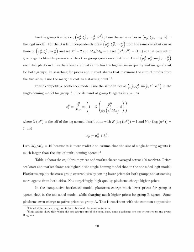
In the competitive bottleneck model I use the same values as(µAjt, ξ

Ajt,mc

Ajt, λ

A, αA)in the

single-homing model for group A. The demand of group B agents is given as

sBj =nBjMB

=

1−G

pBj

ωj

(sAj MA

) |θ

where G(αB)is the cdf of the log normal distribution with E

(log(αB))

= 1 and V ar(log(αB))

=

1, and

ωjt = µBjt + ξBjt.

I set MA/MB = 10 because it is more realistic to assume that the size of single-homing agents is

much larger than the size of multi-homing agents.13

Table 1 shows the equilibrium prices and market shares averaged across 100 markets. Prices

are lower and market shares are higher in the single-homing model than in the one-sided logit model.

Platforms exploit the cross-group externalities by setting lower prices for both groups and attracting

more agents from both sides. Not surprisingly, high quality platforms charge higher prices.

In the competitive bottleneck model, platforms charge much lower prices for group A

agents than in the one-sided model, while charging much higher prices for group B agents. Some

platforms even charge negative prices to group A. This is consistent with the common supposition

12 I tried different starting points but obtained the same outcomes.13Simulations show that when the two groups are of the equal size, some platforms are not attractive to any group

B agents.

20

that platforms make profits from multi-homing agents who join platforms as long as the benefit is

larger than the price they pay. To charge high prices for group B agents, platforms try to attract

as many group A agents as possible with low prices. Despite high prices, more than 30 percent of

group B agents join platforms. Notice that unlike the single-homing model, higher quality platforms

charge lower prices to group A agents.

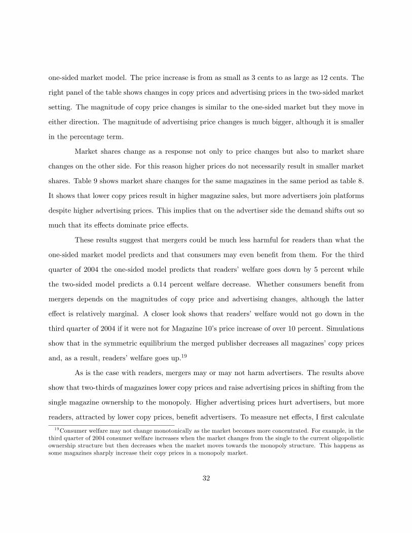
In table 2 I increase the size of group A in both models. In the single-homing model the

size of group A is 10 times larger than that of group B, and in the competitive bottleneck model it

is 20 times larger. The two models react to this change in the opposite ways. In the former model,

platforms increase prices for group A while decreasing prices for group B. Because group B agents

are relatively scarcer, they become more valuable to platforms and are treated more favorably.

Prices to group B agents go down so much that some of them are set below costs. In the latter

model, platforms decrease prices for group A while increasing prices for multi-homing group B

whose willingness to pay for joining them goes up. Despite higher prices, more group B agents join

platforms.

In table 3 I compare the own-price elasticity computed using equation (10) (columns under

Total) with its approximation using equation (11) (columns under Direct). The market size is set

to MA/MB = 10 for both models. The table shows that the approximation is much worse in the

competitive bottleneck model with the magnitude of differences ranging from 31 to 63 percent for

group A and 22 to 45 percent for group B, while it is less than 3 percent in the single-homing model.

The table also shows that platforms do not necessarily set prices at the elastic part of the demand

curve. In the single-homing model all platforms except platform 5 set prices at the inelastic part

for group B. If markets are not two-sided, this cannot be a profit-maximizing pricing strategy.

21

5 Empirical Application: Magazine Advertising

5.1 Data

I use data on magazines published in Germany to estimate the model presented in the previous

sections. Magazines are platforms that serve readers on one side and advertisers on the other side.

Advertisers care about the size of the reader base and readers may or may not like advertising.

I focus on TV magazines, which are categorized by Germany’s Information Association for

the Determination of the Spread of Advertising Media, a non-profit public institution equivalent

to the US Audit Bureau of Circulation. Through its website, this association makes available

quarterly information on copy prices, advertising prices, advertising pages, content pages, and

circulations. Magazines are published at different frequencies. About 65% of TV magazines are

published weekly, 28% bi-weekly and the remaining 7% monthly. The data aggregate the number of

content and advertising pages and the circulation of each issue at a quarterly level, while recording

the average per-issue copy and advertising prices.

Table 4 reports the summary statistics at a yearly level. The table shows a market-share

weighted average (first averaging across magazines in each quarter and then averaging across quar-

ters for each year) and a standard deviation for each variable. For the number of magazines, I

report the number in the first quarter of each year. The advertising price is an average price that

an advertiser pays for one page of advertising in one issue. Magazines charge slightly different

prices depending on whether advertising is in color or not, but I use the average of the two. The

table shows that the copy price and the advertising price are drastically different. Each copy is

sold at around one euro, while one page of advertising is sold at around thirty thousand euros.

I treat all magazines as if they were selling a bundle of issues in each quarter. For example,

I assume monthly magazines are selling a bundle of three issues and bi-weekly magazines are selling

a bundle of seven issues, and so on. This assumption implies that consumers decide which magazine

to read each quarter and buy all issues in a given quarter. To be consistent with this assumption,

22

I multiply the copy price by the number of issues and divide quarterly circulations by the number

of issues in calculating market shares. For example, if the data show a monthly magazine sold 1.5

million copies in a quarter, my assumption implies that 500,000 consumers bought three issues of

this magazine and paid its copy price three times in that quarter.

I make the same assumption for advertisers. If an advertiser chooses to advertise in a

monthly magazine in a given quarter, he buys one advertising page in each issue and pays a per-

page advertising price three times that quarter. This means that the number of advertisers is the

number of advertising pages divided by the frequency. Putting the two sides together, 300 pages of

advertising in a given quarter by a monthly magazine means 300 pages of advertising to consumers

and 100 advertisers to a magazine.14

Magazines, on average, sell about 1.5 million copies, and have about 1,000 content pages

and 250 advertising pages in each quarter. Large standard deviations imply that magazines are

heterogeneous in terms of size and circulation. The average revenue from selling copies is about

1.5 million euros, while its advertising revenue is 7.5 million euros. It is hard to argue that the

copy price covers the publishing cost. However, the low copy price is not unreasonable in the light

of the two-sided market. The magazine may charge below marginal cost to sell as many copies as

possible while charging a high price to advertisers to make profit.

During the sample period seven publishers published 19 magazines in total, seven of which

remained in the market for the entire sample period. Table 4 shows that the number of magazines

increased from 10 to 17 by 2005 and dropped to 15 in 2006 and stayed at that level until the end of

the sample period. However, the market became much more concentrated in the late 2000s. In 1992

six publishers published ten magazines, adding five more magazines by 2000. Then, Gong Verlag

GmbH & Co. KG (GVG), which had been publishing a weekly magazine DieZwei and a biweekly

magazine TVdirekt, sold its magazines to WAZ Verlagsgruppe (WAZ). In 2002 Michael Hahn Ver-

14An alternative approach is to assume that consumers and advertisers make decisions for each issue. Under thisassumption I should make slight modifications in calculating market shares as well as the number of content andadvertising pages consumers “consume". However, it does not significantly change empirical results.

23

lag (MHV) entered the market with a monthly magazine nurTV and soon exited the market in

2005, selling its magazine to WAZ. In 2004 Hubert Burda Media (HBM) took over Verlagsgruppe

Milchstrasse’s (VM) two magazines. Thus, from 2006 only four publishers, Axel Springer Ver-

lagsgruppe (ASV), Bauer Media KG (BMK), HBM and WAZ, remained in the market.15 These

publishers publish a mixture of different frequency magazines. For example, WAZ publishes two

weekly magazines, one bi-weekly magazine and one monthly.

These publishers also publish magazines in other magazine segments such as women, busi-

ness and politics, adult, automotive, etc. An exception is WAZ, which only publishes women’s

magazines and pet magazines other than TV magazines. I exploit this multi-segment feature in

constructing instrumental variables. For example, the prices of magazines in different segments

that are published by the same publisher can be used as IVs for the price variable, because they

are likely to be correlated through common publisher cost factors but demand shocks are unlikely

to be correlated across segments.

5.2 Demand Estimation: Competitive Bottleneck

I assume that consumers choose at most one TV magazine title per quarter and consumer i′s

indirect utility of purchasing magazine j in period t is

uAijt = xjtβ − λpAjt + ξjt + εijt

where xjt is a vector of observed magazine attributes, pAjt magazine copy price, ξjt unobservable

attribute and demand shock and εijt an idiosyncratic taste shock with type I extreme value dis-

tribution. x includes the magazine fixed effect, the time effect, the number of content pages and

the number of advertising pages. Both the copy price and the advertising pages are endogenous

variables that are correlated with the unobservable attribute.15Two magazines published by Hubert Burda Media are excluded from the sample from 2006 because their attribute

data are missing. This explains a drop in the number of magazines from 17 to 15 in 2006 in table 4.

24

An advertiser, whose type is αBi , buys an advertising page if its net profit is positive. The

advertising profit is defined as

πBijt = αBi ωjtnAjt − pBjt

where pBjt is price magazine j charges to an advertiser, nAjt the number of readers for magazine j,

and ωjt a per-reader profitability of one page advertising. I assume that its advertising decision

regarding one magazine is independent of its decision regarding another.16 Thus, there is no direct

competition between magazines to attract advertisers and each magazine acts as a monopolist

towards advertisers. However, there is still an indirect competition between magazines as long as

readers care about (like or dislike) advertising. Given the distribution of advertiser type, F (α|θ),

the number of advertising pages in magazine j, nBj , is determined by

nBjt =

(1− F

(pBjt

ωjtnAjt|θ))

MB

where MB the number of advertisers in the market and F (θ) is assumed to be the lognormal

distribution with the mean parameter 0 and the variance parameter 1.4. Notice that the distribution

parameters are not estimable and should be fixed as part of normalization.17 Thus, estimating

advertisers’ demand is equivalent to imputing the mean benefit (profitability) that advertisers

receive from advertising in magazines, i.e., ω, and projecting it on characteristics space. I discuss

how this normalization affects demand estimates below.

I use the generalized method of moment to simultaneously estimate the following system

of demand equations

log (sjt)− log (s0t) = xjtβ − λpAjt + ξjt (18)

log (ωjt) = wjtγ + ejt (19)

16 In my opinion the competitive bottleneck model describes advertisers better than the two-sided single-homingmodel. The latter model assumes that advertisers select only one magazine for advertising. Nevertheless, I stillestimate this model in the appendix for the sake of comparison.17 I explain why I choose these values in the next section.

25

where w includes the magazine fixed effect, the time effect and the number of content pages.

Moment conditions are that the demand residuals in the two equations,(ξjt, ejt

), are not correlated

with the number of content pages, the time effects, and the mean magazine quality for readers and

advertisers, i.e. the magazine fixed effects. In addition, I use the same and rival publishers’

average copy price and advertising pages in other magazine segments such as women’s magazines,

automotive magazines, etc. as instrumental variables. An identifying assumption is that copy prices

and advertising pages are correlated across magazine segments because of common cost shocks but

demand shocks are not correlated across magazine segments.

Table 5 shows estimation results, and in the appendix I estimate the model using alternative

specifications for the advertiser profit function. The number of potential readers is set to 40 million

and the number of potential advertisers is set to 200. Both numbers are set to exceed per-period

maximum copy sales and advertising pages respectively. Notice that advertising pages reported

in table 4 are the aggregated number for each quarter and a frequency-adjusted advertising page

is no larger than 150 pages. The magazine fixed effects and the time effects are included in all

estimations but not reported.

The first column shows OLS results for equations (18) and (19) respectively. In equation

(18) the price coeffi cient is negative but statistically insignificant. Both the advertising page and

the content page coeffi cients are positive and significant at the 5 percent level. In equation (19) the

content page coeffi cient is negative and significant. The R-square is 0.96 for the former equation

and 0.91 for the latter.

The second column shows the system IV results. I use (Z′Z)−1 as a weighting matrix where

Z is an IV matrix. In the first equation both the price coeffi cient and the advertising page coeffi cient

change significantly. The former goes down from -0.017 to -0.135 and becomes significant and the

latter goes up from 0.116 to 0.208. The positive advertising page coeffi cient implies that readers

like advertising in TV magazines. The fact that the advertising coeffi cient goes up with IVs does

not necessarily mean that the advertising page variable is negatively correlated with the demand

26

residual. When there are two endogenous variables, it is hard to predict the sign of inconsistency in

the OLS estimates because it is driven by how strongly the two endogenous variables are correlated

with the error term. I test if the instruments used for the first equation are weak IVs with the first

stage F-test. The F-statistics are 24.43 for the price variable and 24.84 for the advertising page

variable.

The last column shows the GMM results, using the inverse of the variance of the moment

conditions as the weighting matrix. The weighting matrix is optimal such that standard errors are

smallest under the current moment conditions. The price coeffi cient goes down little further to

-0.155 but the advertising page coeffi cient hardly changes. The content page coeffi cient does not

change across the columns. I test the overidentifying restrictions and accept them with the test

statistics close to zero.

The magazine fixed effects show that popular magazines do not necessarily have higher

per-reader profitability for advertisers. A correlation between a quality ranking for readers and a

quality ranking for advertisers is -0.45 using the system IV estimates and -0.29 using the GMM

estimates. For example, the “lowest profitable" magazine for advertisers, i.e., BMK’s tvpur, in both

estimations is estimated to be the fourth or fifth highest quality for readers. This suggests that

magazine quality not captured by the size of reader basis is also important in explaining advertising

price differences across magazines.

Different parameter values of the advertiser distribution (i.e., F (θ)) mainly affects the

constant term of the advertising demand equation. When the variance parameter varies from 0.5

to 3 with the mean parameter fixed, the constant term decreases from 1.702 to -0.628, but the

other estimates hardly change. For example, the content page coeffi cient changes from -0.103 to

-0.115. Different market sizes have similar effects. As the number of potential advertisers increases

from 150 to 500, the constant term decreases from 1.126 to 0.175 while the other estimates hardly

change. However, their impact on markup is more substantial, and I discuss it in more detail below.

27

5.3 Elasticity and Market Power

Table 6 summarizes price elasticities calculated from the demand estimates. The left panel shows

the own-price elasticities in the one-sided model (∂SAj∂pAj

pAjsAjand

∂SBj∂pBj

pBjsBj) which do not account for the

feedback loop following a price change. The right panel shows the price elasticities in the two-

sided model including the own-price elasticities for readers (∂sAj∂pAj

pAjsAj) and advertisers (

∂sBj∂pBj

pBjsBj) and

the cross-group price elasticities (∂sAj∂pBj

pBjsAjand

∂sBj∂pAj

pAjsBj). The latter measures a percent change in the

number of readers (advertisers) with respect to one percent change in the advertising (copy) price.

Compared to the one-sided model, the own-price elasticities go up (in the absolute term) by about

4 percent.

The cross-group elasticities show that advertisers are much more sensitive to a price change

on the other side. The median cross-group elasticity with respect to a copy price(∂sBj∂pAj

pAjsBj

)is -2.58

while it is -0.04 with respect to an advertising price(∂sAj∂pBj

pBjsAj

). This implies that given the size of

the two groups, the markup on the reader side is much more heavily adjusted than the markup on

the advertiser side. To see this, plug the median elasticities into equations (14) and (15) .

(pAj − cAj

)= 0.59pAj − 1.53

(pBj − cBj

) nBj

nAj(pBj − cBj

)= 0.70pBj − 0.03

(pAj − cAj

) nAj

nBj

These equations show that, given the group size, the markup on the reader side is adjusted by 1.53

times of the markup on the advertiser side, while the markup on the advertiser side is adjusted

by a small fraction (0.03) of the markup on the other side. Of course, the group size, which is

substantially different, is another determinant of the markup.

Whether readers like or dislike advertising changes the sign of the cross-group elasticity and

advertisers’cross-price elasticity among platforms. If readers dislike advertising, ∂sAj /∂pBj becomes

positive and ∂sBj /∂pBk , j 6= k become negative. If readers are indifferent about advertising, both

28

∂sAj /∂pBj and ∂s

Bj /∂p

Bk , j 6= k become zero. As mentioned above, although pricing for advertisers

is modeled as monopolistic, the cross-group interaction makes advertisers’ cross-price elasticity

(among platforms) non-zero, i.e.(∂sBj /∂p

Bk

)(pBk /s

Bj

)6= 0, j 6= k,. However, its magnitude is

so small (the mean cross elasticity is less than 0.001) that its impact on advertising pricing and

markups are negligible.

Table 7 reports per-issue marginal costs and markups. I report per-issue estimates to make

them comparable with prices reported in table 4. On the left panel I report marginal costs and

markups in the one-sided model where platforms maximize profits on each side separately. The

reader-side estimates imply the median marginal cost for producing an over 100-page magazine

is 0.40 euros and it costs less than 0.60 euros to produce a 200-page magazine (the 5th quintile

magazine). The median markup is 62 percent with close to 80 percent of magazines having higher

than a 50 percent markup. The median markup in the one-sided advertising market is 73 percent

with the mean markup equal to 84 percent.

On the right panel I report marginal costs and markups that account for the two-sidedness.

Very different markup structures are seen on the reader side when the advertising side is accounted

for. Although demand estimates do not change significantly, publishers’profit-maximizing behav-

iors are drastically different. The median cost is now 3.39 euros, which results in a negative markup

(-2.39 euros). In fact, 90 percent of magazines are estimated to incur a loss from selling their mag-

azines. However, this loss is fully recovered from selling advertising space. Magazines, on average,

earn about 20,000 euros from selling one advertising page. The average percentage markup is 83

percent, slightly lower than the one-sided model estimate. Combining the two sides, magazines,

on average, make about 65,000 euros per issue with 445,000 euro loss from selling magazines and

510,000 euro profit from selling advertising space.

However, magazines do not always incur a loss from selling their copies. Six magazines

made profits on the readers’side in at least one quarter during the sample period. Four of these

magazines are published by BMK, which owns the highest number of magazines. This suggests

29

that a publisher can still set magazine prices above costs when it has substantial market power.

Nevertheless, this is not a common phenomenon. It only happens to 11 percent of all observations,

and in any period no more than two magazines make profits from selling copies.

The estimated profits show that the advertising profit is almost perfectly negatively corre-

lated with the copy-sale profit. For six publishers, a correlation between these two profits is lower

than -0.90. This means that an increase in the advertising profit almost always accompanies a

decrease in the copy-sale profit. This is consistent with the simulation in section 4 that shows that

a platform with a higher advertising profit incurs a larger loss on the reader side.

Notice that even if readers dislike advertising, the markup results do not change in a

fundamental way. In particular, negative advertising preference makes the advertising markup

higher because magazines want to charge more to advertisers to compensate readers’ disutility,

which makes estimated marginal costs lower for the same observed prices. This implies that the

markup structure is mainly determined by magazines who act as “monopolists" towards advertisers

and advertisers who are willing to pay a lot of money to interact with readers.

While the market size and the parameter (variance) values of the advertiser distribution

mainly affect the constant term in the demand estimation, their impact on markups is more sub-

stantial and how I set their values deserves more explanation. I use 40 million, about a half of the

German population, as the market size for readers to include all potential readers of TV magazines

in Germany. The market size for advertisers is less straightforward to set, but my assumption

about how advertisers make decisions restricts the number of advertisers to be no less than the

maximum advertising pages per issue which is 147. My choice of 200 advertisers, therefore, means

that 53 potential advertisers never advertised in any TV magazines during the sample period. A

lower number increases markup but not substantially.

A reasonable range for the variance of the advertiser distribution, given the market sizes

set above, is between 1 and 1.7. When it is 1, the markup on the advertising side is so low that

five out of seven publishers make negative profits over the entire sample period. When it is 1.7, all

30

publishers make positive profits but the average markup is close to one. My choice of 1.4 is the

lowest value that makes all publishers earn positive profits over the entire sample period.

5.4 Merger Simulations

In this section I analyze how equilibrium prices and market shares (the number of participations)

change when the market becomes more concentrated. In particular, I focus on the shift from the

single magazine ownership to the monopoly (one publisher owning all magazines). Since this change

is from one extreme to the other, it is supposed to result in the most drastic change among any

other possible ownership changes. As the benchmark case I do the same exercise for the one-sided

logit model. The comparison will shed light on how mergers in the two-sided market differ from

the one-sided market.

The observed markets are oligopolistic with three publishers owning two-thirds of TV

magazines. I use the magazine-level markup and cost reported in the previous section for the

current market structure. For the two hypothetical market structures I plug these cost estimates

into the markup equations (equations (14) and (15)) to find new equilibrium prices and market

shares. The search algorithm consists of two parts. While an outer part searches for prices that

satisfy the markup equations with a different ownership structure, an inner part searches for market

shares that satisfy equations (8) and (9) simultaneously for given prices.18

Results show that copy prices can either increase or decrease in the two-sided market,

while they always increase in the one-sided market. Advertising prices can also either increase or

decrease but always move in the opposite direction from copy prices. Given a market (a quarter)

the merged publisher decreases copy prices (and increases advertising prices) for about two-thirds

of magazines.

Table 8 shows price changes for the third quarter of 2004 as an example. I report results

on 10 magazines out of 17 in that quarter. The left panel shows changes in copy prices in the

18As mentioned above, Brouwer’s fixed point theorem guarantees the existence of these shares. Although there canbe multiple sets of shares that satisfy the demand equations, it does not seem to occur in my exercise.

31

one-sided market model. The price increase is from as small as 3 cents to as large as 12 cents. The

right panel of the table shows changes in copy prices and advertising prices in the two-sided market

setting. The magnitude of copy price changes is similar to the one-sided market but they move in

either direction. The magnitude of advertising price changes is much bigger, although it is smaller

in the percentage term.

Market shares change as a response not only to price changes but also to market share

changes on the other side. For this reason higher prices do not necessarily result in smaller market

shares. Table 9 shows market share changes for the same magazines in the same period as table 8.

It shows that lower copy prices result in higher magazine sales, but more advertisers join platforms

despite higher advertising prices. This implies that on the advertiser side the demand shifts out so

much that its effects dominate price effects.

These results suggest that mergers could be much less harmful for readers than what the

one-sided market model predicts and that consumers may even benefit from them. For the third

quarter of 2004 the one-sided model predicts that readers’welfare goes down by 5 percent while

the two-sided model predicts a 0.14 percent welfare decrease. Whether consumers benefit from

mergers depends on the magnitudes of copy price and advertising changes, although the latter

effect is relatively marginal. A closer look shows that readers’welfare would not go down in the

third quarter of 2004 if it were not for Magazine 10’s price increase of over 10 percent. Simulations

show that in the symmetric equilibrium the merged publisher decreases all magazines’copy prices

and, as a result, readers’welfare goes up.19

As is the case with readers, mergers may or may not harm advertisers. The results above

show that two-thirds of magazines lower copy prices and raise advertising prices in shifting from the

single magazine ownership to the monopoly. Higher advertising prices hurt advertisers, but more

readers, attracted by lower copy prices, benefit advertisers. To measure net effects, I first calculate

19Consumer welfare may not change monotonically as the market becomes more concentrated. For example, in thethird quarter of 2004 consumer welfare increases when the market changes from the single to the current oligopolisticownership structure but then decreases when the market moves towards the monopoly structure. This happens assome magazines sharply increase their copy prices in a monopoly market.

32

the surplus of the average advertiser on magazine j by

E(αBi |i ∈ j

)ωjn

Aj − pBj

where E(αBi |i ∈ j

)denotes the average value of αBi conditional on joining magazine j. Then I

multiply the average surplus by the number of advertisers joining each magazine.

Results show that the average surplus goes up on magazines that raise advertising prices.

Since these magazines attract more advertisers, advertisers’ total surplus also goes up. For the

third quarter of 2004, the increase is 30 percent at Magazine 7 and 15 percent at Magazine 1.

On the other hand, advertisers’surplus goes down on magazines that lower advertising prices, but

fewer magazines do so and changes are less than 10 percent. For the whole market, as a result,

advertisers’aggregate surplus increases by 1.7 percent.20

6 Conclusions

In this paper I develop structural models of two-sided markets where two groups of agents interact

through oligopolistic platforms and estimate platform markups using TV magazine data in Ger-

many. My models have two key features of the two-sided market. First, both groups care about

the presence of the other group, so the cross-group externalities are present on both sides. Second,

platforms set different prices for each group to maximize joint profits from both sides. To account

for these cross-group externalities I treat market share equations as a system of implicit functions

where platform prices are control variables and the market share of both sides are endogenous

variables. I use the implicit function theorem to compute the price elasticities and recover platform

markups.

The empirical results show that most of the magazines set copy prices below marginal

costs to attract readers and make profits from selling advertising space. When the advertising

20An important assumption in this exercise is that the merged publisher keeps all magazines and do not changetheir other characteristics. Rysman (2004) shows that advertisers are better off with more platforms.

33

side is ignored, the same demand estimates imply high markups on the reader side. Counterfactual

exercises show that platform mergers do not necessarily increase copy prices and, as a result, readers

may not necessarily be worse off in more concentrated markets.

Some extensions are worth consideration. First, I assume there is no intra-platform compe-

tition but it can be an important factor in agents’membership decisions. For example, advertisers’

platform valuation may go down with the number of other advertisers on the same platform. This

is equivalent to congestion, or negative externalities, in network industries. With intra-platform

competition a few interesting issues arise including whether platforms would choose exclusive deal-

ing and how prices on the other side are affected. Second, I only consider the fixed membership

fee in this paper but incorporating more flexible fee structures, such as charging usage fees, are

certainly important topics for future empirical research.

34

References

[1] Argentesi, E. and L. Filistrucchi (2007), “Estimating Market Power in a Two-sided Market:The Case of Newspapers," Journal of Applied Econometrics, 22, 1247-1266.

[2] Armstrong, M. (2006), “Competition in Two-sided Markets," RAND Journal of Economics,37, 668-691.

[3] Berry, S. (1994), “Estimating Discrete Choice Models of Product Differentiation," RANDJournal of Economics, 25, 242-262.

[4] Berry, S., J. Levinsohn, and A. Pakes (1995), “Automobile Prices in Market Equilibrium,"Econometrica, 63, 841-890.

[5] Chandra, A. and A. Collard-Wexler (forthcoming), “Mergers in Two-Sided Markets: An Appli-cation to the Canadian Newspaper Industry," Journal of Economics and Management Strategy.

[6] Jeziorski, P. (2011), “Merger Enforcement in Two-sided Markets," unpublished manuscript,Johns Hopkins University.

[7] Jin, G. and M. Rysman (2010), “Platform Pricing at Sports Card Conventions," unpublishedmanuscript, Boston University.

[8] Kaiser, U. and J. Wright (2006), “Price Structure in Two-Sided Markets: Evidence from theMagazine Industry," International Journal of Industrial Organization, 24, 1-28.

[9] Rochet, J.-C. and Tirole, J. (2003), “Platform Competition in Two-Sided Markets," Journalof the European Economic Association, 1, 990-1029.

[10] Rochet, J.-C. and Tirole, J. (2006), “Two-Sided Markets: A Progress Report," RAND Journalof Economics, 37, 645-667.

[11] Rosen, J. (1965), “Existence and Uniqueness of Equilibrium Points for Concave n-personGames," Econometrica, 33, 520-534.

[12] Rysman, M. (2004), “Competition between Networks: A Study of the Market for YellowPages," Review of Economic Studies, 71, 483-512.

[13] Rysman, M. (2009), “The Economics of Two-Sided Markets," Journal of Economic Perspective,23, 125-143.

[14] Weyl, G. and A. White (2010), “Imperfect Platform Competition: A General Framework,"unpublished manuscript, Harvard University.

35

Table 1: Average Price and Market Share in Equilibrium

Logit Model Single-Homing Competitive Bottleneck

Group A Group A Group B Group A Group B

Platform Price Share Price Share Price Share Price Share Price Share

1 0.748 0.126 0.679 0.136 0.664 0.131 0.263 0.032 0.574 0.300

2 0.932 0.124 0.852 0.131 0.815 0.133 0.118 0.061 1.820 0.282

3 1.089 0.122 1.028 0.130 0.989 0.138 -0.262 0.137 5.453 0.365

4 1.237 0.128 1.174 0.136 1.150 0.142 -0.569 0.289 13.929 0.408

5 1.418 0.117 1.335 0.137 1.336 0.135 -0.649 0.458 26.303 0.409

The market size is set to MA/MB=1 for the single-homing model and MA/MB=10 for the competitivebottleneck model.

36

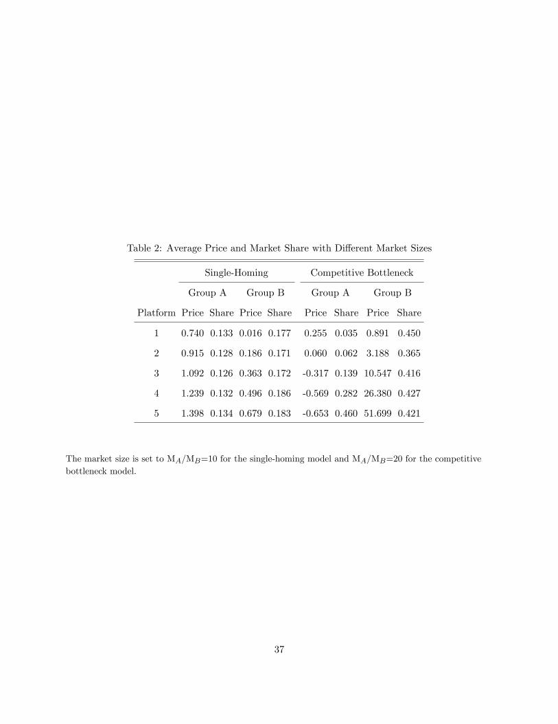
Table 2: Average Price and Market Share with Different Market Sizes

Single-Homing Competitive Bottleneck

Group A Group B Group A Group B

Platform Price Share Price Share Price Share Price Share

1 0.740 0.133 0.016 0.177 0.255 0.035 0.891 0.450

2 0.915 0.128 0.186 0.171 0.060 0.062 3.188 0.365

3 1.092 0.126 0.363 0.172 -0.317 0.139 10.547 0.416

4 1.239 0.132 0.496 0.186 -0.569 0.282 26.380 0.427

5 1.398 0.134 0.679 0.183 -0.653 0.460 51.699 0.421

The market size is set to MA/MB=10 for the single-homing model and MA/MB=20 for the competitivebottleneck model.

37

Table 3: Average Own-Price Elasticities

Single-Homing Competitive Bottleneck

Group A Group B Group A Group B

Platform Direct Total Direct Total Direct Total Direct Total

1 -1.283 -1.312 -0.292 -0.299 -0.850 -1.115 -1.585 -1.930

2 -1.604 -1.637 -0.468 -0.476 -0.975 -1.336 -1.460 -1.880

3 -1.913 -1.954 -0.683 -0.695 -0.965 -1.494 -1.107 -1.589

4 -2.161 -2.210 -0.885 -0.904 -0.900 -1.466 -0.953 -1.379

5 -2.427 -2.483 -1.168 -1.192 -0.774 -1.255 -0.949 -1.273

The market size is set to MA/MB = 10 for both models.

38

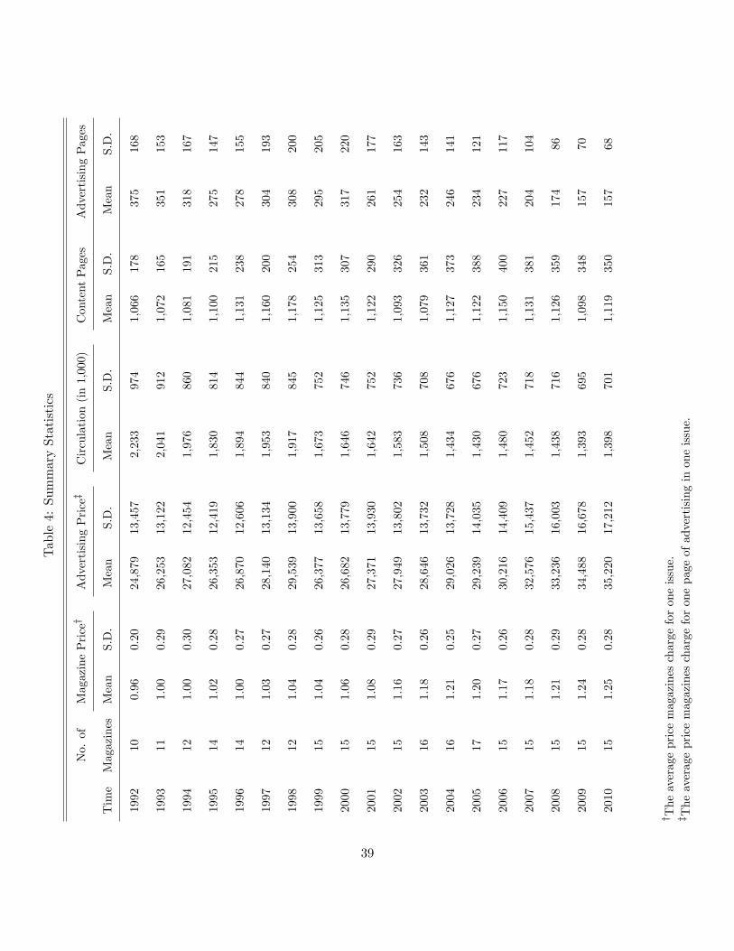
Table4:SummaryStatistics

No.of

MagazinePrice†

AdvertisingPrice‡

Circulation(in1,000)

ContentPages

AdvertisingPages

Time

Magazines

Mean

S.D.

Mean

S.D.

Mean

S.D.

Mean

S.D.

Mean

S.D.

1992

100.96

0.20

24,879

13,457

2,233

974

1,066

178

375

168

1993

111.00

0.29

26,253

13,122

2,041

912

1,072

165

351

153

1994

121.00

0.30

27,082

12,454

1,976

860

1,081

191

318

167

1995

141.02

0.28

26,353

12,419

1,830

814

1,100

215

275

147

1996

141.00

0.27

26,870

12,606

1,894

844

1,131

238

278

155

1997

121.03

0.27

28,140

13,134

1,953

840

1,160

200

304

193

1998

121.04

0.28

29,539

13,900

1,917

845

1,178

254

308

200

1999

151.04

0.26

26,377

13,658

1,673

752

1,125

313

295

205

2000

151.06

0.28

26,682

13,779

1,646

746

1,135

307

317

220

2001

151.08

0.29

27,371

13,930

1,642

752

1,122

290

261

177

2002

151.16

0.27

27,949

13,802

1,583

736

1,093

326

254

163

2003

161.18

0.26

28,646

13,732

1,508

708

1,079

361

232

143

2004

161.21

0.25

29,026

13,728

1,434

676

1,127

373

246

141

2005

171.20

0.27

29,239

14,035

1,430

676

1,122

388

234

121

2006

151.17

0.26

30,216

14,409

1,480

723

1,150

400

227

117

2007

151.18

0.28

32,576

15,437

1,452

718

1,131

381

204

104

2008

151.21

0.29

33,236

16,003

1,438

716

1,126

359

174

86

2009

151.24

0.28

34,488

16,678

1,393

695

1,098

348

157

70

2010

151.25

0.28

35,220

17,212

1,398

701

1,119

350

157

68

† Theaveragepricemagazineschargeforoneissue.

‡ Theaveragepricemagazineschargeforonepageofadvertisinginoneissue.

39

Table 5: Demand Estimation Results

Variable OLS System IV GMM

Readers Constant -7.250∗ -5.604∗ -5.111∗

(0.235) (0.640) (0.612)

Copy Price -0.017 -0.135∗ -0.155∗

(0.012) (0.033) (0.032)

Ads Page 0.116∗ 0.208∗ 0.204∗

(0.011) (0.030) (0.028)

Content Page 0.062∗ 0.069∗ 0.060∗

(0.007) (0.008) (0.008)

Advertisers Constant 0.727∗ 0.727∗ 0.900∗

(0.160) (0.242) (0.233)

Content Page -0.102∗ -0.102∗ -0.110∗

(0.010) (0.012) (0.011)

The market size for readers is set to 40 million and the market size for advertisers to 200.The magazine fixed effects and the time effects are included in all estimations.Standard errors are reported in parenthesis.∗significant at the 5 % level.

40

Table 6: Price Elasticity

One-Sided Two-Sided∂SAj∂pAj

pAjsAj

∂SBj∂pBj

pBjsBj

∂sAj∂pAj

pAjsAj

∂sBj∂pBj

pBjsBj

∂sAj∂pBj

pBjsAj

∂sBj∂pAj

pAjsBj

Median -1.64 -1.38 -1.69 -1.43 -0.04 -2.58

Mean -1.68 -1.31 -1.77 -1.37 -0.05 -2.32

20% QU∗ -1.21 -1.02 -1.30 -1.11 -0.02 -1.04

80% QU -2.12 -1.60 -2.17 -1.63 -0.08 -3.28

The market size for readers is set to 40 million and the market size for advertisers to 200.A refers to the reader side and B refers to the advertiser side.∗QU refers to a quintile.

41

Table 7: Magazine Market Power

One-Sided Two-Sided

Markets Cost Markup % Markup Cost Markup % Markup

mc (p−mc) (p−mc) /p mc (p−mc) (p−mc) /p

Readers Median 0.40 0.51 0.62 3.39 -2.39 -2.26

Mean 0.29 0.79 0.78 4.23 -3.15 -2.58

20% QU∗ 0.13 0.50 0.48 1.56 -5.48 -4.52

80% QU 0.54 1.09 0.83 6.83 -0.74 -0.88

Advertisers Median 2,761 13,733 0.73 3,061 13,580 0.72

Mean 1,031 21,446 0.84 1,329 21,148 0.83

20% QU 599 5,469 0.63 950 5,283 0.61

80% QU 7,890 32,115 0.98 7,999 31,582 0.96

The market size for readers is set to 40 million and the market size for advertisers to 200.∗QU refers to a quintile.

42

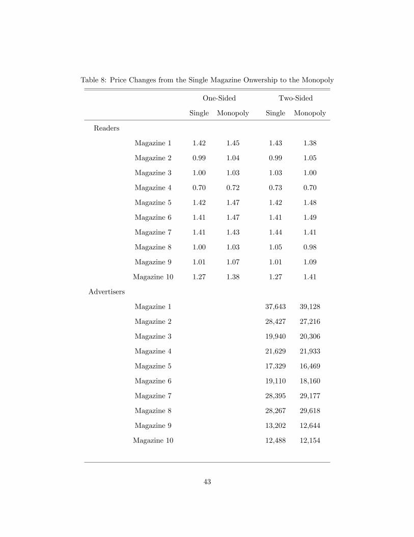
Table 8: Price Changes from the Single Magazine Onwership to the Monopoly

One-Sided Two-Sided

Single Monopoly Single Monopoly

Readers

Magazine 1 1.42 1.45 1.43 1.38

Magazine 2 0.99 1.04 0.99 1.05

Magazine 3 1.00 1.03 1.03 1.00

Magazine 4 0.70 0.72 0.73 0.70

Magazine 5 1.42 1.47 1.42 1.48

Magazine 6 1.41 1.47 1.41 1.49

Magazine 7 1.41 1.43 1.44 1.41

Magazine 8 1.00 1.03 1.05 0.98

Magazine 9 1.01 1.07 1.01 1.09

Magazine 10 1.27 1.38 1.27 1.41

Advertisers

Magazine 1 37,643 39,128

Magazine 2 28,427 27,216

Magazine 3 19,940 20,306

Magazine 4 21,629 21,933

Magazine 5 17,329 16,469

Magazine 6 19,110 18,160

Magazine 7 28,395 29,177

Magazine 8 28,267 29,618

Magazine 9 13,202 12,644

Magazine 10 12,488 12,154

43

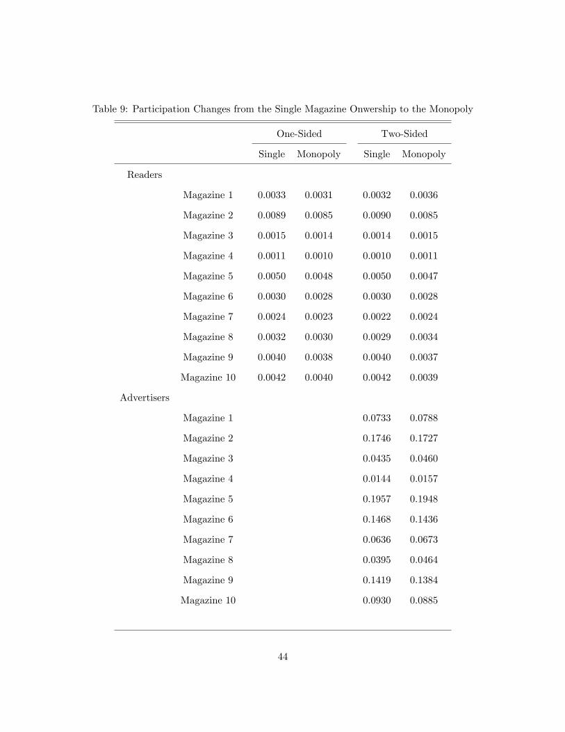
Table 9: Participation Changes from the Single Magazine Onwership to the Monopoly

One-Sided Two-Sided

Single Monopoly Single Monopoly

Readers

Magazine 1 0.0033 0.0031 0.0032 0.0036

Magazine 2 0.0089 0.0085 0.0090 0.0085

Magazine 3 0.0015 0.0014 0.0014 0.0015

Magazine 4 0.0011 0.0010 0.0010 0.0011

Magazine 5 0.0050 0.0048 0.0050 0.0047

Magazine 6 0.0030 0.0028 0.0030 0.0028

Magazine 7 0.0024 0.0023 0.0022 0.0024

Magazine 8 0.0032 0.0030 0.0029 0.0034

Magazine 9 0.0040 0.0038 0.0040 0.0037

Magazine 10 0.0042 0.0040 0.0042 0.0039

Advertisers

Magazine 1 0.0733 0.0788

Magazine 2 0.1746 0.1727

Magazine 3 0.0435 0.0460

Magazine 4 0.0144 0.0157

Magazine 5 0.1957 0.1948

Magazine 6 0.1468 0.1436

Magazine 7 0.0636 0.0673

Magazine 8 0.0395 0.0464

Magazine 9 0.1419 0.1384

Magazine 10 0.0930 0.0885

44

Appendix I: Alternative Specifications for the Advertiser Profit FunctionIn this section I explore alternative specifications for the advertiser’s profit function. The firstalternative specification (Alt I ) to consider is

πBijt = αBi ωjt − pBjt

where ωjt denotes the magazine quality perceived by advertisers. Recall that in the original specifi-cation the magazine quality perceived by advertisers is at a per-reader level so that the advertisingbenefit for magazine j is αBi ωjtn

Ajt. In this alternative specification, the advertising benefit for

magazine j is αBi ωjt, and ωjt is a function of njt and other magazine characteristics.A nice feature of this specification is that advertisers’valuation on the number of readers

can be directly estimated. One plausible function form for ωjt is

ωjt =(nAjt)τ

exp (wjtγ) exp (ejt) .

where ωjt is positive only when nAjt is non-zero, keeping an essential feature that magazines arevaluable to advertisers only through readers. I treat nAjt as an endogenous variable that can becorrelated with ejt and use the number of readers in other magazine segments as instrumentalvariables. One may consider the original specification as fixing τ at 1.

The second alternative specification (Alt II ) to consider is

πBijt = ωjtnAjt − pBjt + rijt

where ωjt is the per-reader magazine quality and rijt is an i.i.d. random variable distributednormal with mean zero. In this specification the mean valuation of a magazine is the same acrossadvertisers, but each advertiser draws a random profit shock in each period.

An advertiser buys an advertising page in magazine j only if rijt > ωjtnAjt − pBjt such that

a portion of advertisers who buy an advertising page in magazine j is

nBjtMB

=

(1− Φ

(ωjtn

Ajt − pBjtσ

))

where Φ (.) is the cumulative distribution function of the standard normal distribution and σ is thevariance of rijt..

The last alternative specification (Alt III ) is

πBijt = ωjt − pBjt + rijt

where ωj denotes the magazine quality. This specification combines the first and the second al-ternative specifications. ωjt is a function of njt and other magazine characteristics as in the firstalternative specification, and the mean valuation of a magazine is the same across advertisers as inthe second alternative specification.

Table 10 shows the GMM estimates of the advertiser-side magazine demand for the three

45

alternative specifications. The variance parameter is fixed at 1.4, the same value as in the originalspecification. For comparison I put the original specification estimates in the second column (Base).The table shows that in the first alternative specification (Alt I) the coeffi cient on the log of thenumber of readers is positive and statistically significant. This means that the larger the readerbase is, the larger the advertiser’s revenue. This verifies the assumption of the original specification,but the larger-than-one coeffi cient implies that the advertiser’s revenue increases with the readerbase much faster than in the original specification.

The average magazine quality implied by the estimates of the magazine dummy variables(not reported in the table) is slightly different compared to the original specification. The fivehighest quality and the four lowest quality magazines are the same in both specifications, but themagazines that are ranked the 11th and the 8th respectively in the original specification are rankedthe 6th and the 13th in the alternative specification.

There are more drastic changes in the average magazine quality in the second alternativespecification (Alt II ). For example, the second highest quality magazine in the base specificationis ranked the 10th, and the 13th ranked magazine in the original specification is ranked the 4th.However, the highest quality magazine and the two lowest quality magazines do not change.

Interestingly, the magazine quality ranking is exactly the same except for one magazinebetween the second and the third alternative specifications. However, the coeffi cient on the logof the number of readers is close to zero and statistically insignificant in the third alternativespecification (Alt III ). It is in sharp contrast with the result of the first alternative specificationand misleadingly implies that advertisers do not put much value on the number of readers theiradvertising can reach. This suggests that putting the advertiser heterogeneity additively in theprofit function may not be a correct modeling choice.

Appendix II: Estimation in the Two-Sided Single-Homing ModelIn the two-sided single-homing model advertisers choose only one magazine for advertising. Theymake a magazine choice to maximize their profits. Advertiser i’s profit function of advertising inmagazine j is

πBij = Rij − pBjwhere Rij is the advertiser’s revenue and pBj is a per-page advertising price the magazine charges.Assuming that the advertiser’s revenue is a linear function of magazine characteristics includingthe market share on the reader side,

πBij = xjβB − pBj + ξBj + εBij

where xj includes observed magazine characteristics, ξBj denotes the mean effect of unobserved mag-azine characteristics and demand shocks on the advertiser’s revenue and εBij is an i.i.d. idiosyncraticprofit shock which I assume is distributed type I extreme value.

A system of demand equations to estimate is equations (16) and (17) in section 3. Theonly difference is that the price coeffi cient for advertisers is set to -1. The share of readers isan endogenous variable and I use the same type of instrumental variables as in estimating thecompetitive bottleneck model. I divide both the copy price and the advertising price by 10,000.

46

Otherwise, the exponential function in the advertiser-side market share blows up. Dividing the copyprice does not affect demand estimates other than scaling up the price coeffi cient. Also, I makethe market size on the advertiser side larger than the sum of advertising pages across magazinesin a given period to be consistent with the assumption in the two-sided single-homing model thatadvertisers choose only one magazine.

Table 11 shows estimation results in the two-sided single-homing model. The reader-sideestimates using the system IV and the GMM estimation techniques are statistically significantand their magnitudes are similar to those in table 5 except for the advertising share variable.This difference mainly comes from using the advertising share variable rather than the number ofadvertising pages. All coeffi cients, nevertheless, change in the same direction as in table 5. On theadvertising side the reader share variable is added in estimation. Its coeffi cient is positive, meaningthat advertisers appreciate a larger reader base, and its magnitude goes down with instrumentalvariables, implying that it is positively correlated with demand shocks. Recall that the pricecoeffi cient is fixed at -1 so the reader share variable is the only endogenous variable.

One thing to notice is that the reader share coeffi cient is about four times larger thanthe advertising share coeffi cient. Recall that in the two-sided single-homing model, platformscharge a lower price to a smaller size group if the two group’s valuation of the other group is thesame. However, the data show that advertisers, the smaller size group, pay much higher pricesthan readers do. The larger reader share coeffi cient resolves this inconsistency by showing thatadvertisers appreciate readers more than readers appreciate advertisers.

These demand estimates seem to suggest that the two-sided single-homing model can be alsoused to describe the media advertising. In fact, the magazines usually charge below-cost copy pricesto readers and make profits from advertisers in this model, as advertisers’appreciation of readers ismuch greater than readers’appreciation of advertisers. However, a loss on the reader side is muchless adequately compensated by a profit on the advertiser side. That is because magazines competeto attract advertisers instead of behaving as monopolists towards them. Moreover, magazines withlarger reader bases make smaller profits. This is in sharp contrast to the result in the competitivebottleneck model where magazines with larger reader bases are able to earn higher profits fromadvertisers.21 These results render support to using the competitive bottleneck model in describingmagazine advertising.

21The coeffi cient correlation between the two sides’markups is -0.92 in the competitive bottleneck model while itis 0.18 in the two-sided single-homing model.

47

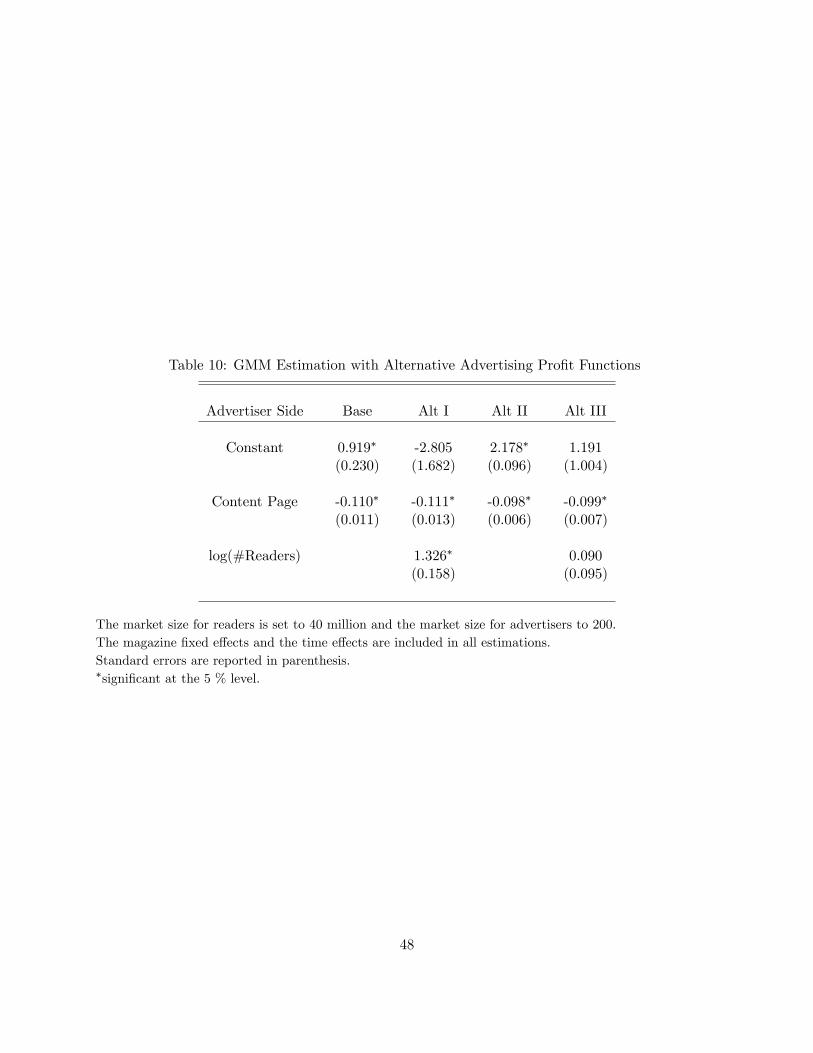
Table 10: GMM Estimation with Alternative Advertising Profit Functions

Advertiser Side Base Alt I Alt II Alt III

Constant 0.919∗ -2.805 2.178∗ 1.191(0.230) (1.682) (0.096) (1.004)

Content Page -0.110∗ -0.111∗ -0.098∗ -0.099∗

(0.011) (0.013) (0.006) (0.007)

log(#Readers) 1.326∗ 0.090(0.158) (0.095)

The market size for readers is set to 40 million and the market size for advertisers to 200.The magazine fixed effects and the time effects are included in all estimations.Standard errors are reported in parenthesis.∗significant at the 5 % level.

48

Table 11: Demand Estimation in the Two-Sided Single-Homing Model

Variable OLS System IV GMM

Readers Constant -7.001∗ -5.500∗ -5.092∗

(0.232) (0.494) (0.471)

Copy Price -0.020 -0.122∗ -0.137∗

(0.012) (0.028) (0.027)

Ads Share 0.465∗ 0.875∗ 0.799∗

(in %) (0.042) (0.113) (0.110)

Content Page 0.063∗ 0.070∗ 0.063∗

(0.007) (0.008) (0.007)

Advertisers Constant -2.362∗ -2.244∗ -2.224∗

(0.261) (0.382) (0.368)

Reader Share 4.814∗ 3.657∗ 2.857∗

(in %) (0.203) (0.607) (0.498)

Content Page -0.121∗ -0.117∗ -0.126∗

(0.016) (0.015) (0.014)

The market size for readers is set to 40 million and the market size for advertisers to 5,000.The magazine fixed effects and the time effects are included in all estimations.Standard errors are reported in parenthesis.∗significant at the 5 % level.

49