1

ESTIMATING THE ANCILLARY BENEFITS OF GREENHOUSE GAS MITIGATIONPOLICIES IN THE US

by Dallas BURTRAW and Michael A. TOMAN

1. Introduction

To a large extent, policies for limiting emissions of greenhouse gases (GHGs) have been analyzed interms of their costs and potential for reducing the rate of increase in atmospheric concentrations ofthese gases. However, actions to slow atmospheric GHG accumulation could have a number of otherimpacts, such as a reduction in conventional environmental pollutants. The benefits (or costs) thatresult are often referred to as “ancillary” to the benefits and costs of GHG abatement (though there iscontroversy surrounding this terminology and the underlying concepts).

A failure to adequately consider ancillary benefits and costs of GHG policy could lead to an inaccurateassessment of the overall impacts of mitigation policies. In particular, not accounting for ancillarybenefits and costs would lead to an incorrect identification of a “no regrets” level of GHG mitigation.It also could lead to the choice of an unnecessarily expensive policy because of its failure to fullyexploit potential ancillary benefits.

In this paper we first review briefly the concept of ancillary benefit, as it is developed in more detail inother papers in this proceedings and elsewhere in the literature. The concept turns out to besurprisingly difficult to define precisely. What is considered an ancillary benefit depends on the scopeof policies being considered, the policy objectives being pursued, and the identity of the interestsbeing served. That said, however, we describe what we believe is a serviceable definition of ancillarybenefits from the perspective of evaluating GHG mitigation policies within the “Annex I” countrieswho would have emission limitation obligations under the Kyoto Protocol. We focus on mitigation inthis paper, while acknowledging that adaptation policies also could have ancillary effects (forexample, improved surveillance of tropical diseases could yield immediate health dividends;protection of coastal lands could harm wetland habitats in the more immediate term).

2

Having established a workable definition, we then turn to issues related to measuring ancillarybenefits. To illustrate these issues, we consider how lower GHG levels resulting from less fossil fueluse could also reduce various “criteria” air pollutants (as defined in the U.S. Clean Air Act). Recentcomprehensive studies of electricity fuel cycles indicate that the lion’s share of the environmental andpublic health effects of fuel and technology choices in electricity generation stem from air emissions.These effects typically total about 85 percent or more of the quantifiable environmental concerns,excluding climate change and species biodiversity (Lee et al., 1995; Rowe et al., 1995; EC, 1995).Thus, focusing on the air-health pathway of ancillary benefits is likely to provide a fairly reliablepicture of total ancillary benefits, though controversy remains regarding the magnitudes of non-healtheffects.

We find in our review that estimates of ancillary health benefits for the US vary considerably.Previous estimates have ranged from over $60 per ton of carbon reduced (or greater in one specialcontext) to $3 per ton. The dispersion of US estimates reflects partly underlying parametricuncertainty, in particular the economic valuation of health impacts. There also are several importantdifferences in the identification of baselines, in particular the effect of current and future regulatorystandards for conventional pollutants (see the paper by Morgenstern). Still other differences arise inthe scale of modeling, in particular the distinction between more detailed sector-specific analyses (inpractice these involve the electricity sector), and specific geographic locations, in contrast toeconomy-wide estimates based on much simpler modeling of environmental impacts.

For a variety of reasons that are evident below, we have much more confidence in more conservative(lower) estimates of ancillary benefits (especially those drawn from more detailed models) comparedto estimates that equal or exceed the costs of GHG control. Ancillary benefits could offset a significantfraction of the costs of carbon reduction with moderate GHG policies. It also may be possible toorient GHG abatement policies in certain ways to take greater advantage of ancillary benefits.However, the considerable variation in baseline assumptions and in policy scenarios, coupled withuncertainty about the size of ancillary benefits, leads to tremendous variation in estimates, precludingidentification of a single “best estimate” of their magnitude.

In the next section of the paper we briefly review our working definition of ancillary benefit. SectionIII contains a review of estimates from a number of US studies. Section IV provides a more detaileddiscussion of methods and results from ongoing research at RFF on ancillary benefits from GHGrestrictions in the electricity sector. This approach reflects what might be seen as a “best practice” inthe development and use of detailed methodology for linking GHG policies to changes in conventionalpollutant emissions, ambient consequences, health effects assessment, and economic valuation.Section 5 interprets and critiques the various estimates presented in Sections 3 and 4. Section 6 offersconcluding remarks and suggestions for further research.

2. Defining and measuring ancillary benefit or cost

2.1 Definitional issues

An ancillary benefit of a GHG mitigation policy is understood by many analysts to refer to a benefit(derived from GHG mitigation) that is reaped in addition to the benefit targeted by the policy, which isreduction in the adverse impacts of global climate change. An ancillary cost would be a negativeimpact experienced in addition to the targeted benefit. The key elements of this definition, and thesources of much of the controversy surrounding the notion of ancillary, are “in addition” and“targeted.”

3

In the context we have used for defining ancillary benefits and costs, the principal policy goal is GHGmitigation in order to reduce adverse climate impacts. Asserting that ancillary benefits are additionalto the benefits of reducing climate change does not mean these benefits are necessarily less important,or that other policy goals are less important than addressing climate change. Benefits that are ancillaryto climate change could be bigger in magnitude and more salient for the affected citizens and theirdecision makers. Our definition simply puts ancillary benefits in a certain policy context.

That policy context can be and is debated. Developing countries have argued with justification thatthey have more pressing development and environmental needs than reducing their GHGs. In thisbroader policy context, what we refer to as ancillary benefits could be considered as “co-benefits” ofpolicies designed to promote various objectives. Our own view is that when discussing climatechange policies, the benefits and costs targeted by the policies should be considered as thoseassociated with GHG mitigation and climate change risk reduction; other benefits and costs should betreated as ancillary in the sense we have defined the term above, but not given short shrift.

Some more specific but related considerations that arise in defining ancillary benefits and costsinvolve the scope of what is included in the calculation and the perspective of the decision makerevaluating benefits and costs. A number of kinds of impacts can be considered when evaluatingancillary benefits and costs. Much of the emphasis in these calculations has been on near-term healthimpacts in relatively close proximity to the GHG mitigation (for example, reduced incidence of lungdisease in the same area as a coal-fired power plant if that plant is used less as a consequence of GHGmitigation measures), but a variety of other impacts also could be important.

For example, ecological systems could be affected by reductions in the flow of conventional pollutants(for example, less fossil fuel use could mean less nitrogen oxide deposition into water bodies).Reduced pollutants also could reduce some direct costs, such as maintenance of infrastructure andpollution-related reductions in crop yields. Also, traffic accidents could be reduced from less drivingor slower traffic speeds. Reduced traffic could lower road maintenance costs. Similarly, increasedforest areas dedicated to carbon sequestration could increase recreational opportunities and reduceerosion. GHG policies could also stimulate technical innovation.

Ancillary costs can arise if energy substitution leads to other health and environmental risks (e.g. fromnuclear power, uncontrolled particulate emissions from biomass combustion, or use of diesel fuel inlieu of gasoline, since diesel fuel has lower carbon emissions but greater emissions of otherpollutants). Better building insulation can add to indoor air pollution, including radon, and switchingfrom coal to gas raises the specter of fugitive emissions of methane, a more potent greenhouse gasthan CO2. Also, policies that promote reforestation could encourage destruction of old growth naturalforests because younger forests allow more carbon storage. Further, GHG mitigation policies couldmainly redirect innovation efforts away from other productive activities, rather than increasing it. Inaddition, relatively expensive GHG mitigation policies could have some negative side effects onhealth by reducing the resources available to households for other health-improving investments.

4

An economic perspective on ancillary benefits sees them as part of a larger concern with economicefficiency, as typically expressed in measures of aggregate benefits and costs. From this perspective,it is important not to isolate ancillary benefit and cost information from other relevant benefit and costinformation associated with GHG policy. Ancillary benefits of a policy could be substantial, but theyare nonetheless a questionable achievement if the cost of garnering these benefits is much larger.Often ancillary benefits are expressed in terms of a monetary measure per ton of carbon not emitted tothe atmosphere as a consequence of the mitigation policy. Expressed this way, ancillary benefits (andcosts) can be compared to the cost of mitigation. This is usually a meaningful and useful comparison,since ancillary benefits often (but not always) occur on the same relatively shorter-term time scale asmitigation costs, while the benefits of reducing climate change will be realized in the more distantfuture.

A final related point is that the scope and magnitude of ancillary benefits and costs depends on theperspective of the decision maker as to what constitutes policy relevant impacts. From the perspectiveof a hypothetical global decision maker concerned with global social well-being, ancillary benefits andcosts are important wherever they are incurred. From this perspective it thus is important to considerhow a redistribution in the location of GHG mitigation could affect ancillary benefits and costs.

In particular, policy mechanisms like international emissions trading or the Clean DevelopmentMechanism will redistribute ancillary impacts toward those countries undertaking more GHGmitigation. And efforts by Annex I alone to mitigate GHGs could have collateral effects in developingcountries not bound by quantitative emissions limits, in that lower energy prices in internationalmarkets will stimulate some additional energy use and associated local environmental effects in thosecountries. On the other hand, for an Annex I decision maker evaluating the benefits and costs of GHGmitigation policies in his or her own jurisdiction, the relevant ancillary benefits and costs are likely toconsist primarily of those affecting individuals in that political jurisdiction. Cross-boundary spilloverslike those illustrated above are relevant for the Annex I decision maker only to the extent that a senseof ethical responsibility or altruism motivates a broader concern for the spillovers.

Still another perspective would be adopted by the developing country decision maker contemplatinginvolvement in the Clean Development Mechanism. In this case, the primary benefits in terms ofimportance for the developing country considering hosting a GHG-reducing investment are likely tobe the benefits that are ancillary to the GHG control according to our definition of the term.

2.2 Empirical challenges

To calculate ancillary benefits and costs over time, one must compare two hypothetical situations.The first is a baseline scenario without any modification of GHG mitigation policy. This is sometimesreferred to as “business as usual,” but this term is somewhat misleading since over time, the status quocan change even without modification of GHG policies. The baseline is compared to an even morehypothetical scenario that involves changing the current and future “state of the world” by modifyingGHG mitigation. To carry out this exercise in practice means addressing a number of challenges.

5

How the baseline is defined crucially affects the magnitude of ancillary benefits and costs generatedby a change in GHG mitigation policy. The paper by Morgenstern in this proceedings identifies anumber of important influences on the baseline. One is the status of non-climate policies. This can bevividly illustrated with two environmental examples. Suppose that even in the absence of climatepolicy, conventional air pollutants are expected to drop sharply because of trends in policies for theregulation of conventional pollutants. (Note that such a trend requires not just tougher standards overtime but also a maintenance or increase in the degree of compliance with those standards.) In thiscase, we would expect the incremental benefits from a reduction of conventional air pollutants in thewake of tougher GHG controls to be smaller than if the increased GHG controls were being applied toa dirtier baseline environment.

The second example involves the establishment of total emission caps for conventional pollutants, likethe cap on sulfur dioxide (SO2) from power plants in the U.S. If such a cap is imposed, then a strongerGHG mitigation policy will not have an effect on the total emissions of conventional pollutants unlessa much tougher GHG policy is imposed, so tough that it leads to polluters reducing conventionalemissions below the legal cap. What would be affected in less stringent cases is the location of theconventional emissions, which can have an important effect on the size of exposed populations, etc.This example also illustrates the need for careful cost and benefit accounting when calculatingancillary benefits and costs.

Aside from the interaction of GHG policies and conventional pollutant policies over time, there areseveral other important elements in specifying the baseline. All the factors driving the evolution of theeconomic system are included in this list. The state of technology will affect the energy andemissions-intensity of economic activity. The size and location of the population, and the volume andlocation of total economic output, will affect both the scale of physical impacts on the environmentand the risks posed to the population. Finally, the status of natural systems is also part of the baseline;it indicates the sensitivity of humans and ecological resources to changes in conventional pollutants.

Another important set of influences on estimates of ancillary benefits and costs include the scale ofanalysis, the level of aggregation, and the stringency of the GHG policy being considered. Asdiscussed below, we find that estimates of ancillary health benefits from reduced conventional airpollutants (expressed as dollars per ton of carbon release avoided) tend to get smaller when theanalysis shifts from an aggregate perspective to one that considers more carefully the effects of GHGpolicies on specific sectors at specific locations. These latter analyses appear better able to model thedistribution of gains and losses, and the behavioral responses to GHG policies. As for the stringencyof GHG policy, we would expect that a stronger GHG program will generate successively smallerincrements in ancillary benefits and more ancillary costs as other risks decline relative to baselinelevels.

One must remain critical of the assessment of the ancillary impacts themselves. In the area ofconventional air pollutants and human health, which has received more research support than others,there nonetheless continues to be considerable uncertainty about how a change in ambientenvironmental conditions will affect health endpoints (for example, how many fewer cases of diseasewill result from somewhat cleaner air), and how much society values these changes. We illustrate theeffects of these uncertainties below. The uncertainties are especially acute and troubling when onetries to use studies of impacts and valuations from developed countries to assess ancillary benefits indeveloping countries with lower incomes, different health status and infrastructure, and differentcultural norms. Other health and non-health ancillary environmental benefits and costs are even lessresearched or understood.

6

Finally, we note that ancillary benefits may not just physical, but may be economic. One importantexample is illustrated by returning to the example of the cap on SO2 from power plants in the U.S.Though there may be no ancillary reductions in emissions of SO2 as noted, there will be an effect onthe cost of compliance under the SO2 program. Under the cap, a facility that reduces its SO2 emissionsmakes emission allowances available for another facility, displacing the need for abatementinvestment at that facility. If a carbon policy reduces the use of coal in electricity generation, it willlead to a reduction in the demand for SO2 allowances, thereby avoiding investment in SO2 abatement.In addition, many studies of the cost of carbon reduction use historically based carbon abatement costestimates that do not incorporate the effects of the SO2 cap and thereby overstate the opportunity costof carbon reductions. For instance, the imposition of controls on a conventional pollutant such as SO2

may reduce the cost advantage that coal has over gas for electricity generation. Layered on top of acontrol on SO2, the reduction of carbon emissions (achieved by substitution from coal to gas) would beless expensive than it would appear were the model to ignore SO2 controls. Hence, the baseline forcomparison of ancillary benefits with costs would be inconsistent, in a potentially important way.

3. Adverse human health effects of conventional air pollutants: a review of US studies

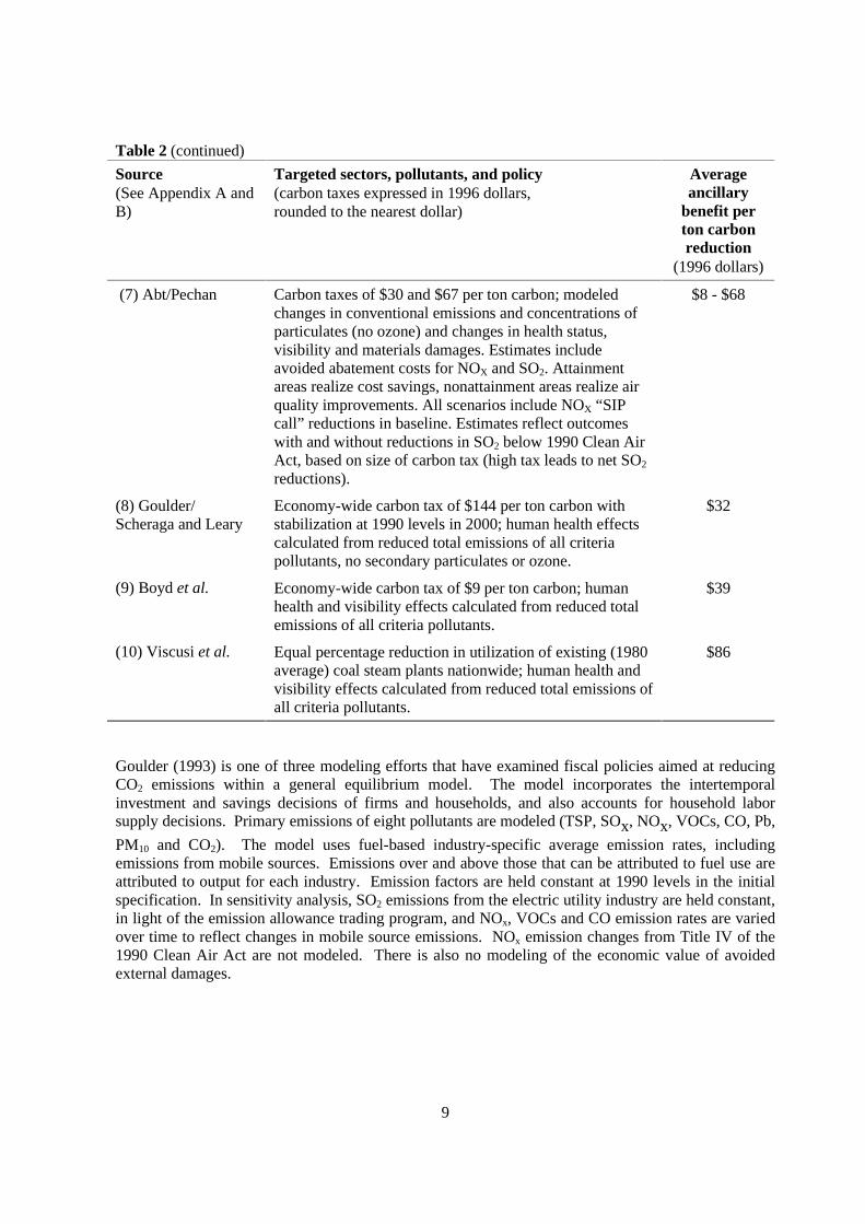
Table 1 summarizes a variety of models and assumptions used to calculate ancillary benefit estimates.References for the estimates are given in Appendix A to this paper. Table 2 summarizes the estimatesthat are achieved in some of these studies, expressed in the common metric of dollars per ton reductionof carbon emissions. In every case the original studies that produced these data identified a wide rangeof possible estimates around the midpoint estimate for ancillary benefits per ton of carbon emissionreduction that we report. Lower and upper bounds for each estimate vary from the midpoints by afactor of 2 to 10 or more.

7

Table 1. Description of previous studies of air pollution reduction benefits from greenhouse gaslimitations

Study(*) and/ormodel exercised(**)See Appendix A andAppendix B Model type Carbon policy or target

Conventional pollutantsand impacts considered

Does baselineinclude 1990

Clean AirAmendments

(including SO2

cap)?Goulder (1993)*/Scheraga and Leary(1993)*

Dynamic generalequilibrium

Economy-wide carbon or Btutax to return total US CO2

emissions to 1990 levels in2000 (emissions rise thereafter)

TSP, SO2, NOx, VOCs, CO,Pb, PM10 (no secondaryparticulates or ozone); humanhealth effects only

No (considered insensitivityanalysis)

Jorgenson et al.(1995)*

Dynamic generalequilibrium

No specified GHG target; fueltaxes set to internalizeconventional air pollutionexternalities

See entry for Viscusi et al.(1992) below

No

Boyd, Krutilla,Viscusi (1995)*

Static generalequilibrium

Energy taxes set either to“optimally internalize”conventional externalities or toexploit all “no regrets”possibilities

See entry for Viscusi et al.(1992) below

No

ICF (1995)* Partialequilibriumregional model ofelectricity sector

Voluntary programs underClimate Change Action Plan

CO, TSP, VOCs, NOX andPM10 (SO2 assumed constant,no secondary particulates);health effects only

Yes

Dowlatabadi et al.(1993)*

Partial equlbriumregional model ofelectricity sector

Technology policy to improveefficiency and reduce emissions

TSP, NOX, and SO2 (nosecondary particulates)

No

Viscusi et al.(1992)*

Valuation only,average fornation

Estimated average damages perunit of emission for variouspollutants

TSP, SO2, NOX, VOCs, CO,Pb, PM10 (damage fromsecondary particu-lates andozone inferred and attributedto primary pollutants); humanhealth and visibility effects

No

EXMOD(Hagler-Bailly,1995)**

Detailedelectricity sectorfor NY State,atmospherictransport andvaluation

Facility specific emissions anddamages; used for sensitivityanalysis of other studies

TSP, SO2, NOX, VOCs, CO,Pb, PM10, (second-aryparticulates and ozonemodeled); all human health,visibility and otherenvironmental effects

Yes

PREMIERE(Palmer et al.,1996)**

Regionalelectricity sector,atmospherictransport andvaluation

Regionally specific emissionsand damages; sensitivityanalysis of other studies

Only NOX (and secondarynitrates) modeled; humanhealth effects only

Yes

HAIKU (Burtraw,et al. 2000)*

Same, detailedelectricity sectormodel

Same NOX and SO2 (and secondarypollutants modelled); SO2 capbinding; human health only

Yes, additionalreductions

Abt/Pechan(McCubbin et al.1999)*

Same, for alleconomic sectors

Same; special attention toavoided abatement costs

SO2, NOX, PM, CO, O3;Visibility, materials analysed;only health monetized

Yes, additionalreductions

Lutter and Shogren(1999)*

Los Angeles Same, no sensitivity analysis;special attention to avoidedabatement costs

Only PM Yes, additionalreductions

8

Table 2. Comparisons of estimates of ancillary benefits per ton of carbon reduction

Source(see Appendix A and B)

Targeted sectors, pollutants, and policy(carbon taxes expressed in 1996 dollars,

rounded to the nearest dollar)

Averageancillary

benefit perton carbonreduction

(1996 dollars)

(1) HAIKU/TAF

Nationwide carbon tax of $25 per ton carbon in electricitysector, analyzed at state level; only health effects fromNOx changes valued, including secondary particulates,excluding ozone effects. Range of estimates reflect with,and without, NOx “SIP call” reductions included inbaseline.

$2-$5

(2) ICF/PREMIERE

Nationwide Motor Challenge voluntary program(industry), analyzed at regional level; only health effectsfrom NOx changes valued, including secondaryparticulates, excluding ozone effects.

$3

(3) Dowlatabadi et al./PREMIERE

Nationwide seasonal gas burn in place of coal,analyzed at regional level; health effects from NOx

changes valued using PREMIERE, including secondarynitrates, excluding ozone effects

$3

(4) EXMOD Reduced utilization of existing coal steam plant at asuburban New York location; only PM, NOx and SO2

(under emission cap) changes valued (based on 1992average emissions), including secondary particulates andozone effects; all health, visibility and environmentaleffects that could be quantified are included.

$26

(5) Coal/PREMIERE Equal percentage reduction in utilization of all existing(1994) coal plants in U.S. analyzed at state level; onlyhealth effects from NOx changes valued, includingsecondary particulates and excluding ozone.

$8

(6) Coal/PREMIERE/RIA

Equal percentage reduction in utilization of all existing(1994) coal plants in U.S. analyzed at state level; only NOx

related mortality changes valued, including secondaryparticulates and excluding ozone, using new EPA RIAestimates of impacts and valuations.

$26

9

Table 2 (continued)

Source(See Appendix A andB)

Targeted sectors, pollutants, and policy(carbon taxes expressed in 1996 dollars,rounded to the nearest dollar)

Averageancillary

benefit perton carbonreduction

(1996 dollars)

(7) Abt/Pechan Carbon taxes of $30 and $67 per ton carbon; modeledchanges in conventional emissions and concentrations ofparticulates (no ozone) and changes in health status,visibility and materials damages. Estimates includeavoided abatement costs for NOX and SO2. Attainmentareas realize cost savings, nonattainment areas realize airquality improvements. All scenarios include NOX “SIPcall” reductions in baseline. Estimates reflect outcomeswith and without reductions in SO2 below 1990 Clean AirAct, based on size of carbon tax (high tax leads to net SO2

reductions).

$8 - $68

(8) Goulder/Scheraga and Leary

Economy-wide carbon tax of $144 per ton carbon withstabilization at 1990 levels in 2000; human health effectscalculated from reduced total emissions of all criteriapollutants, no secondary particulates or ozone.

$32

(9) Boyd et al. Economy-wide carbon tax of $9 per ton carbon; humanhealth and visibility effects calculated from reduced totalemissions of all criteria pollutants.

$39

(10) Viscusi et al. Equal percentage reduction in utilization of existing (1980average) coal steam plants nationwide; human health andvisibility effects calculated from reduced total emissions ofall criteria pollutants.

$86

Goulder (1993) is one of three modeling efforts that have examined fiscal policies aimed at reducingCO2 emissions within a general equilibrium model. The model incorporates the intertemporalinvestment and savings decisions of firms and households, and also accounts for household laborsupply decisions. Primary emissions of eight pollutants are modeled (TSP, SOx, NOx, VOCs, CO, Pb,

PM10 and CO2). The model uses fuel-based industry-specific average emission rates, includingemissions from mobile sources. Emissions over and above those that can be attributed to fuel use areattributed to output for each industry. Emission factors are held constant at 1990 levels in the initialspecification. In sensitivity analysis, SO2 emissions from the electric utility industry are held constant,in light of the emission allowance trading program, and NOx, VOCs and CO emission rates are variedover time to reflect changes in mobile source emissions. NOx emission changes from Title IV of the1990 Clean Air Act are not modeled. There is also no modeling of the economic value of avoidedexternal damages.

10

The base case in the Goulder model, which ignores the SO2 cap and other expected changes inemissions, is extended by Scheraga and Leary (1993) to estimate a level of CO2 emission reductionssufficient to return to 1990-level emissions in the year 2000, about 8.6 percent relative to the base caseprojection in the model.1 When a carbon tax is used for this purpose, the emission reductions forconventional pollutants range from 1.4 percent (VOC) to 6.6 percent (NOX).

Goulder et al. append estimates of the monetary value of avoided health damage culled from a varietyof sources, including EPA Regulatory Impact Assessments from the 1980s. They estimate reductionsin VOCs, SOx, particulates and NOx emissions resulting from the carbon tax, yielding benefits in therange of $300 million to $3 billion, with benefits about 33 percent greater for a Btu tax. Although theauthors do not make this comparison, a rough estimate of the cost of this level of taxation suggests thatabout one quarter of the cost of the policy is offset by the value of criteria air pollutant reductions.

Jorgenson et al. (1995) provides another dynamic general equilibrium model that includes adjustmentsfor projected technical change on an industry basis. Externalities related to global climate change andto criteria air pollutants and acid rain resulting from energy use are modeled. The climate damagevalues rise over time to reflect the relationship between accumulated greenhouse gases and damages.The 1990 Clean Air Amendments are not reflected in the study. The externality values for reductionsin conventional pollutants are unit values adapted from the survey of cost-benefit studies and otherresearch compiled in Viscusi et al. (1992), adjusted downward to reduce the estimate of prematuremortality associated with sulfur oxides.

These energy related externalities are converted into tax rates under several different scenariosaccommodating a range of values for climate and conventional externalities, and they are internalizedinto prices through ad valorem energy taxes, ranging from a 1 percent markup for natural gas to a197% markup for coal, under their benchmark scenario. The authors also investigate the performanceof several strategies for recycling revenue from an energy tax. Their results conform with a “strongform” of the double-dividend hypothesis (Goulder, 1995). This means they find negative (gross)economic costs (that is, positive benefits) from the energy taxes, as measured by equivalent variationdefined over goods, services and leisure, when the revenues are used to displace property taxes orcapital taxes, even when environmental benefits are not considered.2 Further, when revenue isrecycled by reducing labor taxes, in which case the net economic cost of abatement is positive, theauthors find the net benefits of the policy to be positive once reduced conventional pollutant damagesare taken into account (not including climate related benefits).

1 However, after year 2000 emissions are allowed to increase, which has an implication for the type of

abatement measures employed.2 This strong finding is contradictory to a large share of recent studies on the subject (Oates, 1995;

Goulder, 1995). The main reason for this result is the large economic cost (marginal cost of funds)assumed to result from the use of property or capital taxes to raise government revenues, compared toother studies, as well as the relatively large economic cost of taxes in general represented in themodel. However, as noted in the text, they find a less striking result when revenues are recycled toreduce labor taxes, which is the usual assumption.

11

Boyd, Krutilla and Viscusi (1995) use a simpler general equilibrium model, with land treated as aseparate factor of production, to consider ad valorem taxes on fuels, with revenues rebated inlump-sum fashion to taxpayers (so there are no gains from recycling revenues to reduce other taxes).Pollutants considered are the same as in Jorgenson et al. (1995) and environmental benefit estimatesare drawn directly from Viscusi et al. (1992). The “optimal” tax levels in the analysis are defined asthose that maximize the sum of benefits from reducing conventional environmental externalities(excluding any benefits from reducing carbon emissions) less the economic costs of the tax.

In the base case the optimal carbon emission reductions are 0.19 billion tons (about 12 percent of totalemissions). The authors report the optimal ad valorem tax on coal is about 45 percent, comparable toa $8/ton carbon charge.3 The authors also identify the “no regrets” level of reduction in the analysis asthe point at which net benefits from internalizing conventional environmental externalities drop tozero. This is equal to 0.5 billion tons (a 29 percent reduction), which would be achieved with a $13tax per ton carbon (leading to a 54 percent ad valorem tax on coal). In the case of a higher substitutionelasticity between energy and other factors of production, the no regrets level of carbon reduction isestimated to be about 0.8 billion tons (49 percent reduction).

Two other modeling efforts are based on frameworks that include considerable detail about theelectricity industry. Holmes et al. (1995) (ICF) use the DEGREES model to examine four out ofapproximately 50 actions identified in the Climate Change Action Plan announced by the ClintonAdministration in 1993, and the impact these actions would have on electricity demand, generation,and associated emissions. These actions include expansion of the Green Lights Program, energyefficient electrical motor systems (Motor Challenge), improvement of hydroelectric generation, andreform of electricity transmission pricing. Pollutants modeled include NOX, SO2, CO, TSP, VOCs,and PM10.

The study examines the change in emissions on a geographic basis, according to North AmericanElectric Reliability Council (NERC) Regions. Regional variation in emission changes stems in largepart from the variation in technologies providing electricity at the margin and that would be affectedby each of the actions. In some regions of the country, for example, gas facilities would be morelikely to be displaced while in other regions coal facilities may be displaced, and these fuels andtechnologies typically have very different emission rates. The study is unique because it examineschanges on a seasonal and time-of-day temporal basis, by modeling changes in the electricity loadduration curve and facility operation. In addition, the study is the most comprehensive in theconsideration of changes in emission rates already destined to occur due to provisions in Title IV ofthe 1990 Clean Air Act Amendments. The study suggests that SO2 emissions will be approximatelyinvariant to the actions that are studied, though the timing of emission reductions under Title IV maybe affected by the policies that were evaluated. Baseline NOx emissions are also projected to fall dueto the requirements of Title IV.

3 We have difficulty replicating their calculations regarding the carbon charges.

12

Dowlatabadi et al. (1993) employ another detailed model of the electric utility system called theEnergy Policy Assessment model to assess emission changes at the regional level. This modelingeffort was based on a 1987 plant inventory, and it did not include changes resulting from the 1990Clean Air Act Amendments. Pollutants that were modeled in addition to CO2 were SO2, NOx andTSP. In common with the ICF model, this model reported results by NERC region. The model wasused to consider technology including seasonal gas burning; use of externality adders in dispatch offacilities; extension of the life of nuclear facilities; elimination of federal subsidies; and improvementof the efficiency of electricity distribution transformers.

A main contribution of the study was to illuminate the potential importance of double-counting ofemission changes when individual policies affect the same endpoints. The emission changes fromthese policies are not additive because the policies taken separately would each capture the samelow-cost substitution opportunities that would not be available in similar degree to the policies takenas a group. The ratio of the emission changes for NOx for the strategies considered collectively is11 percent less than the sum of emission changes when the policies are considered separately in theshort run scenario. The study also illuminates potential perverse effects from technology policy. Forexample, the NOx emissions that could result as people switch to gas use for home and water heatingin response to changes in electricity prices could be greater than the NOx emissions from centralizedelectricity generation sources providing the same energy services. In addition, emissions from gas usein the home are distributed throughout a metropolitan area. This could have greater environmentaldamages than emissions from sources more distant from population centers, potentially offsettingsome of the ancillary benefits from carbon policies.

McCubbin et al. (1999) (Abt/Pechan) is a detailed analysis similar to the HAIKU/TAF analysis thatwe characterize below as “best practice.” McCubbin et al. assume the implementation of carbon taxesand estimate changes in energy consumption by region and sector of the economy. These changes aretranslated into changes in emissions, and then translated into changes in concentrations of particulatesusing a source-receptor matrix. Finally, these are mapped into changes in health status and valued inmonetary terms. The modeling steps are those used in other detailed, peer-reviewed studies conductedby the US EPA. McCubbin et al. paid careful attention to revisions in the US air quality standards inconstructing their baselines. The study accounted for reductions in compliance costs for achievingambient air quality standards in regions of the country that are in attainment of air quality standards, aswell as improvements in air quality and health status in regions that are in nonattainment.

A limitation of the study is that the total carbon reductions that are achieved under the tax is notreported, probably because of the political sensitivity of the question of the cost of achieving carbonreductions in the US. This omission makes estimation of ancillary benefits per ton of carbon reduceddifficult. In some cases additional reductions of SO2 in the baseline are achieved through new airquality standards that reduce the annual cap. However, when they are not achieved in the baseline,then the carbon policy yields reductions because annual emissions fall below the cap established in the1990 Clean Air Act. This yields the high end estimates they present. We note that the proportion ofSO2 reductions that are achieved relative to carbon reductions is greater than that in HAIKU/TAF.

13

One other study that we do not include in our review of estimates is Lutter and Shogren (1999). Thisstudy offers an analytical description of how changes in carbon emissions affect the emissions of otherpollutants and includes an accounting of the reduction in compliance costs in achieving air qualitystandards for conventional pollutants. This point is embodied in some of the other papers we review.Lutter and Shogren illustrate this point in the special context of Los Angeles where the compliancecost of strict new ambient standards would be especially dramatic. In this case, carbon reductions yieldlarge ancillary benefits of around $300 per ton from reduced compliance costs. The authors point outthat ancillary benefits would have an effect on whether a nation should choose to reduce emissionsdomestically or seek to acquire permits in a trading program.

4. The HAIKU/TAF model: An illustration of best practice

The study by Burtraw et al. (2000), which uses the HAIKU/TAF integrated framework, is one webelieve illustrates best practice (as noted, the methods are similar to those in McCubbin et al. (1999)).Burtraw et al. exercise an electricity market model to predict changes in nitrogen oxides (NOx), sulfurdioxide (SO2), and mercury from moderate carbon policies. These changes are fed through anatmospheric transport and health model to predict changes in health status, and to characterize thesechanges in monetary terms. Additional savings accrue from reduced investment in SO2 abatement inorder to comply with the SO2 emission cap due to the shift away from coal for electricity generationunder a carbon tax.

The study directly addresses three methodological issues that are important to the consideration ofhow GHG mitigation could yield ancillary benefits. These include the characterization of changes inemissions, the characterization of health benefits, and the baseline against which these changes aremeasured.

4.1 Emissions

Burtraw et al. focus exclusively on air emissions and their potential health effects, which as notedaccount for 85 percent or more of the quantifiable environmental concerns in previous studies of theelectricity sector. Also, they focus exclusively the electricity sector. While the electricity sector isresponsible for one-third of carbon emissions presently, the EIA projects that this sector will beresponsible for as much as three-quarters of CO2 emission reductions in the U.S. under potentialimplementation of the Kyoto Protocol (EIA, 1998). Hence, this sector will be especially important asthe least expensive and likely source of reductions under moderate reduction scenarios.

4.2 Health effects

This paper uses the “damage function approach” to focus on estimating the social cost of electricitygeneration from facilities examined on an individual basis. The approach has been used in recentanalyses of environmental impacts of electric power plant siting and operation in specific geographiclocations (Lee et al., 1995; EC, 1995; Rowe et al., 1995). The approach involves an atmospherictransport model linking changes in emissions at a specific geographic location with changes inexposure at other locations. Concentration-response functions are used to predict changes in mortalityand a number of morbidity endpoints, and these changes are valued in monetary terms drawing onestimates from the economics literature.

14

The model accounts for expected changes in population, and for expected changes in income thataffect estimates of willingness to pay for improvements in health status. These are importantconsiderations since population and income trends have greatly outstripped energy prices over the lastcentury. U.S. population is expected to grow by 45 percent over just the next fifty years, whichcoupled with expected income growth, suggests that there will be greater exposure to a given level ofpollution and consequently greater benefits from reducing that pollution (Krutilla, 1967). Thisdemographic consideration suggests that the reported values for conventional pollutants in previousstudies underestimate damage in future years, if all other things are equal.

4.3 The baseline

In a static analysis the baseline can be treated as the status quo, but since climate policy inherently is alonger-term effort, questions arise about projecting energy use, technology investments, and emissionsof GHGs and criteria pollutants with and without the GHG policy. The issue is confounded because ofongoing changes in the standards for criteria air pollutants. If one proceeds on the basis of historicalstandards and ignores expected changes in the standards, the ancillary benefit estimate will overstateenvironmental savings. Indeed, historical emission rates may be ten times the rates that apply for newfacilities. In addition, the recent tightening of standards for ozone and particulates and associatedimprovements in environmental performance over time imply that benefits from reductions in criteriaair pollutants resulting from climate policies will be smaller in the future than in the present.

Burtraw et al. include alternative baselines for NOx controls beyond Phase II of Title IV of the 1990Clean Air Act Amendments. One baseline adds a cap and trade program for the summer months forthe Ozone Transport Commission member states in the northeast. This trading program began in 1999.An alternative adds a cap and trade program for a larger region that includes all the eastern states inthe Ozone Transport Rulemaking Region (the so-called “SIP call region”) affected by the EPA’sSeptember 1998 proposed rule regarding NOx emissions.

Another important example of a regulatory baseline is the cap on SO2 emissions from electricitygeneration in the U.S. A consequence of the current emissions cap is that aggregate SO2 emissionsfrom electric utilities (the major source category in the U.S.) are not likely to change much as a resultof moderate GHG emission reductions such as we describe in this paper. Only if climate policies aresufficiently stringent that utilities substitute away from coal in significant fashion and the long-runannual level of SO2 emissions is less than the annual emissions cap would ancillary benefits fromfurther reductions in SO2 be achieved.

Many previous studies use historical SO2 emission rates and do not incorporate the SO2 emission cap,and hence they overstate the ancillary benefits that may be achieved, at least by moderate climatepolicies. By the same token, however, historically based CO2 abatement cost estimates that do notincorporate the effects of the SO2 cap overstate the opportunity cost of CO2 reductions. For instance,the imposition of controls on a conventional pollutant such as SO2 may reduce the cost advantage thatcoal has over gas for electricity generation. Layered on top of a control on SO2, the reduction of CO2

emissions (achieved by substitution from coal to gas) would be less expensive than it would appearwere the model to ignore the SO2 controls.

Further, there is an ancillary economic saving associated with CO2 reductions, even with a bindingSO2 emissions cap. Under the cap, a facility that reduces its SO2 emissions makes emissionallowances available for another facility, displacing the need for abatement investment at that facility.

15

Burtraw et al. assume the SO2 cap is binding and hence they do not anticipate ancillary benefits fromchanges in SO2 emissions for moderate policies. However, they do anticipate reduced costs ofcompliance with the SO2 cap to result as a consequence of climate policies, and these savings arereflected in expected change in electricity prices and consumer and producer surplus. If new standardsregarding NOx emissions from power plants take the form of a cap and trade program analogous to theSO2 program, but applied only during the summer months, then further emissions in NOx will be lessthan under a performance standard. However, in this case we would expect a greater ancillaryeconomic saving due the avoided abatement investment for NOx controls, analogous to the avoidedabatement investment for SO2 controls under the SO2 cap.

Finally, the issue of baselines is complicated further by the changes in the regulation of the electricityindustry. At the time of this writing (summer 2000) over half of the US population reside in states thathave committed themselves to a path of restructuring that would culminate in a move away from costof service pricing for electricity and toward market-based, marginal cost pricing. This change has thepotential and is expected by many to affect dramatically the emissions of various pollutants. Burtrawet al. adopt a cautious assumption regarding the future regulation of the industry by assuming thattraditional average cost pricing continues in effect in regions that have not committed to marginal costpricing by 2000.

4.4 The models

The study employs an electricity market equilibrium model called HAIKU to simulate marketequilibrium in regional electricity markets and inter-regional electricity trade, with a fully integratedalgorithm for NOx and SO2 emission control technology choice. The model simulates electricitydemand, electricity prices, the composition of electricity supply, inter-regional electricity tradingactivity among NERC regions, and emissions of key pollutants such as NOx, SO2, mercury and CO2

from electricity generation. Investment in new generation capacity and retirement of existing facilitiesare determined endogenously in the model, based on capacity-related “going forward costs.”Generator dispatch in the model is based on minimization of short run variable costs of generation.

Two components of the HAIKU model are the Intra-regional Electricity Market Component and theInter-regional Power Trading Component. The Intra-regional Electricity Market Component solvesfor a market equilibrium identified by the intersection of electricity demand for three customer classes(residential, industrial and commercial) and supply curves for each of three time periods (peak, middleand off-peak hours) in each of three seasons (summer, winter, and spring/fall) within each of13 NERC regions. The Inter-regional Power Trading Component solves for the level of inter-regionalpower trading necessary to equilibrate regional electricity prices (gross of transmission costs andpower losses). These inter-regional transactions are constrained by the assumed level of availableinter-regional transmission capability as reported by NERC.

Technical parameters are set to reflect midpoint assumptions by the EIA and other organizationsregarding technological change, growth in transmission capacity, and a number of other factors. Mostnew investment is in conventional technologies including integrated combined cycle natural gas unitsand gas turbines. Fuel supply is price responsive according to a schedule derived from EIA models.

16

To estimate the potential for carbon emission reductions, Burtraw et al. impose a tax on all emissionsin the industry. This tax is collected through the price of electricity and affects dispatch andinvestment decisions. Tax levels of $10-$50 per metric ton of carbon are far below the EIA’sestimated tax of $348 per metric ton carbon required to achieve Kyoto budgets in 2010 in the absenceof international trading.

The changes in emissions of NOx are fed into the Tracking and Analysis Framework (TAF). TAF is anonproprietary and peer-reviewed model constructed with the Analytica modeling software (Bloydet al., 1996).4 TAF integrates pollutant transport and deposition (including formation of secondaryparticulates but excluding ozone), visibility effects, effects on recreational lake fishing throughchanges in soil and aquatic chemistry, human health effects, and valuation of benefits. All effects areevaluated at the state level and changes outside the U.S. are not evaluated.

Health effects are characterized as changes in health status predicted to result from changes in airpollution concentrations. Impacts are expressed as the number of days of acute morbidity effects ofvarious types, the number of chronic disease cases, and the number of statistical lives lost to prematuredeath. The health module is based on concentration-response (C-R) functions found in thepeer-reviewed literature. The C-R functions are taken, for the most part, from articles reviewed in theU.S. Environmental Protection Agency (EPA) Criteria Documents (see, for example, USEPA 1995,USEPA 1996b). The Health Effects Module contains C-R functions for PM10, total suspendedparticulates (TSP), sulfur dioxide (SO2), sulfates (SO4), nitrogen dioxide (NO2), and nitrates (NO3).The change in the annual number of impacts of each health endpoint is the output that is valued. In thisexercise inputs consist of changes in ambient concentrations of NOx, and demographic information onthe population of interest. The numbers used to value these effects are similar to those used in recentRegulatory Impact Analysis by the USEPA.

4.5 Results

We use the HAIKU/TAF model to evaluate two scenarios, and results from the analysis are presentedin Table 3. (See Burtraw et al. 2000 for a fuller discussion.) In the first scenario, identified asBaseline OTC, NOx standards implemented in the 1990 Clean Air Act are maintained, except for anadditional cap and trade program that applies during the five month summer season in the Northeaststates. A carbon tax of $23 per metric ton of carbon in the year 2010 would yield ancillary benefitsfrom reductions in NOx of $7 for each ton of carbon reduced (1996 dollars). The primary category ofthese benefits is mortality. Morbidity benefits are also significant. Previous analysis (Burtraw et al.,1998) using TAF indicates that the value of visibility improvements are about the same order ofmagnitude as morbidity benefits, but these results are not included here.

4 Each module of TAF was constructed and refined by a group of experts in that field, and draws

primarily on peer reviewed literature to construct the integrated model. TAF is the work of a team ofover 30 modelers and scientists from institutions around the country. As the framework integratingthese literatures, TAF itself was subject to an extensive peer review in December 1995, whichconcluded that “TAF represent(s) a major advancement in our ability to perform integratedassessments” and that the model was ready for use by NAPAP (ORNL, 1995). The entire model isavailable at www.lumina.com\taflist.

17

Measured against the Baseline OTC case, an $83 tax increases ancillary benefits in the aggregate buthas little effect on the value per ton of carbon, which increases slightly to $8. The quantity of carbonemission reductions that are achieved by an $83 tax is proportionately less than that achieved by a$ 23 tax, which illustrates that the marginal abatement cost curve for carbon reductions is convex overthis range. The proportional change in NOx emissions is also less than the change in the tax rates, but itis not strictly tied to changes in carbon emissions. The difference in the ratios of NOx and carbonreductions stem from many factors including cost thresholds for new investment and retirement, andfrom the geographic location of changes in emissions. In other scenarios the benefits per ton fallslightly or stay relatively constant with different levels of a carbon tax.

Table 3. Ancillary health benefits from reductions in NOx emissions resulting for various carbontaxes in the electricity sector in 2010 using HAIKU/TAF (1996 dollars)

Baseline - OTC Baseline - SIP

Level of Carbon Tax ($/metric ton) 23 83 23 83

Emission Reductions (metric tons)

Carbon (millions) 79 214 88 215NOx (thousands) 874 2586 974 2564

NOx Related Health Benefits(million dollars)

Morbidity 115 368 157 388Mortality 437 1,382 585 1460Total 552 1,750 742 1848

NOx Related Health Benefits perTon Carbon (dollars)

Morbidity 1.5 1.7 1.8 1.8Mortality 5.5 6.5 6.6 6.8Total 7.0 8.2 8.4 8.6

We can examine how much of the increase in NOx benefits is related to locational differences ingeneration by comparing the benefits per ton of NOx reduction under the two levels of tax. FromTable 3, the benefits from a reduction in NOx emissions fall from $676 per ton under an $83 carbontax, to $632 per ton of NOx at a $23 carbon tax. This reduction in the benefit per ton of NOx reductionis due in part to difference in the location of reductions and generation technology. In essence, thismeans that the additional sources reacting to the higher carbon tax have different emission rates forNOX and are located in areas where the conversion of NOx to nitrates is less efficient, or where fewerpeople are being exposed to the nitrate concentrations, or both. Taken together, the nonlinearity inemission reductions and in the benefits of those reductions provides an indication of the importance ofusing a regionally disaggregated model to investigate this issue, unlike some of the previous studiesthat are discussed below.

The emission reductions are achieved by a dramatic shift from generation with coal to generation withgas. Table 4 indicates that generation by coal under the $83 tax falls to 39 percent of that in thebaseline. In contrast, generation by natural gas increases to 158 percent of that in the baseline. Thesechanges are achieved in 2010 and result from a policy that is implemented in 2001. The results woulddiffer if the policy were implemented later.

18

Table 4. The ratio of generation under tax to generation under the baseline for each respectivescenario

Baseline - OTC Baseline - SIP

Level of Carbon Tax ($/metric ton) 23 83 23 83

Gas Generation 1.18 1.58 1.22 1.60Coal Generation .79 .39 .77 .40

In an alternative scenario, we consider implementation of a summertime NOX cap and trade programin the larger eastern US (the SIP call region) during the summer months. These results are labeled theBaseline - SIP scenario in Table 3. The estimate of ancillary benefits per ton of carbon reduction underan $83 tax is $8.6 in this setting, and under a $23 tax it is $8.4. Compared to the results for theprevious case, the Baseline - SIP scenario yields a less of a reduction in NOX under an $83 tax butgreater NOX related health benefits and greater benefits per ton of carbon reduction. Again, thisillustrates the importance of specificity in modeling the location of carbon reductions and thetechnology choice. Table 4 reports differences in generation for this scenario as well.

SO2 emissions are presumed to be unchanged in these scenarios for the size of carbon taxes weconsider. However, ancillary savings associated with reduced investment in SO2 abatement thatresults from decreased use of coal in electricity generation would add roughly an additional $3 per tonof carbon emission reductions.

As noted, the results pertain to the year 2010 from policies implemented beginning in 2001. Hence,the cost of the policy is incurred earlier than 2010, but also there are reductions achieved before 2010.The schedule of costs and benefits over time is important in calculating a present discounted value ofancillary benefits, and is discussed in Burtraw et al. Also, the estimates developed under thesescenarios correspond to carbon taxes that reflect the expected marginal cost of carbon abatement. Theaverage cost per ton of carbon reduced will be less than the tax on a per ton basis, and hence ancillarybenefits may come close to justifying the carbon tax at moderate levels. Burtraw et al. discuss the costof the policies in terms of changes in consumer and producer surplus in a manner that can be directlycompared with ancillary benefits, as well as direct benefits of GHG mitigation, though the latter isnotoriously controversial and difficult to quantify.

19

5. Interpretation of the estimates

5.1 General observations

In this section we attempt to compare previous ancillary benefit estimates along a common metric, byexpressing mid-value estimates per ton reduction in carbon emissions where such a calculation can bemade given the information from the studies. In preparing Table 2, we have supplemented the per-tonof carbon estimates directly available from the studies in Table 1 in two ways. The results of theHolmes et al. (1995) study could be used for a geographic analysis of atmospheric transport ofpollution and exposure of the population, and economic valuation of emission changes. However, thiswas not attempted in the report. To supplement this analysis, we fed the emission changes intoPREMIERE, a model that employs a reduced-form atmospheric transport model linked to monetaryvaluation of health impacts at a NERC region level.5 Similarly, we supplement the Dowlatabadi et al.analysis listed in Table 1 by feeding predicted emission changes into PREMIERE. These calculationsare described in more detail in Appendix B.

The comparison of estimates is reported in Table 2, which indicates a large variation across studies intheir mid-range ancillary benefit estimates. Note that in every case there is a wide range of valuesaround the mid-range estimate, which we do not report. Lower and upper bounds for each estimaterange varies from its midpoint by a factor of 2 to 10 or more. Several differences in the modelsaccount for the bulk of the differences in the results. One is the modeling of criteria pollutantemissions reductions. The general equilibrium models have the advantage in predicting emissionschanges in the future because they can account for changes in the quantity of electricity demand andsubstitution among technologies. However, they are likely to have less accuracy for near-termemission changes because they have less detailed modeling of technology.

However, longer-term future changes in pollution standards are not accounted for in any of the studiesassessing GHG policies that we discuss below (including our own). As a practical matter, this meansour estimates of ancillary benefits should be considered more reliable for near-term GHG policies thanfor policies that are actually implemented in the 2008-2012 “commitment period” identified in theKyoto Protocol. Other things equal (which in practice is not the case), we would expect progresstoward improved air quality in the U.S. to reduce ancillary benefits below the amounts shown inTable 2.

The estimation and valuation of effects from emission changes varies among the studies. It isrelatively weak in the general equilibrium models, which do not treat locational differences. Moreaggregated analyses calculate total emissions changes and apply a single unit value to value theavoided health impacts. In contrast, disaggregated models can more precisely model the location ofemissions, their transport through the atmosphere, and the exposure of affected populations. Theseanalyses show that benefits do not have a simple proportional relationship to reduced emissions.Sensitivity analyses show that the above-mentioned aspects are important influences on ancillarybenefits, so the greater precision with which they are calculated in disaggregated models give usgreater confidence in these results.

5 Palmer et al. (1996). PREMIERE is a derivative of the Tracking and Analysis Framework (TAF)

discussed above.

20

Another reason for the difference in per ton benefit estimates is differences in sectoral coverage andcoverage of pollutants or impacts. For example, the estimates presented range from a small voluntaryprogram affecting the electricity sector to estimates for the economy as a whole.

The treatment of the SO2 cap represents another important distinction among the studies. When thecap is binding, emission reductions in one location are made up in another, but emissions at onelocation are likely to reduce the need for investment in SO2 abatement at another location. This isusually not considered in cost estimates for CO2 reduction. For example, our estimates usingPREMIERE and EXMOD (discussed below) incorporate a secondary benefit of about $3 per ton ofcarbon reduction from avoided investment in SO2 abatement stemming from reduced utilization ofcoal. This benefit is likely to be considerably smaller than the health benefit that would be induced iftotal SO2 emissions were reduced by a GHG policy, leading to a reduction in fine sulfate particlesimplicated in increased premature mortality (Burtraw et al., 1998).

An important corollary of this observation is that the marginal ancillary benefits from a smallreduction in GHGs are likely to differ from the marginal benefit from the last unit of GHG reductionin a more aggressive program of aggregate GHG control. Even if the underlying atmospherictransport and health effects models are essentially linear, as the studies presented here implicitly orexplicitly assume, there will be a threshold at the point where GHG control has made the SO2 cap nolonger binding. Beyond this point, health benefits from additional net reductions in SO2 will accrue.

5.2 Comments on the studies

With these thoughts in mind, if one wants to identify the ancillary benefit per ton of carbon reductionsfor a modest carbon abatement program given the presumed baseline conditions, we would place moreconfidence in the first five estimates in Table 2. All of these estimates reflect the impact of GHGreductions in the electricity sector. These estimates reflect the most detailed methodologies, includinglocational differences in emissions and exposures, and they take into account the role of the SO2 cap inlimiting ancillary benefits. Note that these estimates suggest modest ancillary benefits (less than$8 per ton carbon) for studies averaging over the United States as a whole from electricity sector GHGreductions, though benefits could be significantly higher in certain areas (New York).

The first three studies in Table 2 indicate that subtle aspects of behavioral responses to policies tend tomitigate the desired emission reductions.6 The HAIKU/TAF example demonstrates that the location ofcarbon emissions and the choice of technology for generation in response to a carbon tax will varyover time and space. This leads to variation in the value of ancillary health benefits per ton of carbonreduced. Nonetheless, the values in the two scenarios we compare are within a fairly small rangearound $8 per ton of carbon reduction.

6 The Dowlatabadi et al. estimates may exaggerate this effect because they reflect the capital stock circa

1987 and do not reflect improvements in gas technologies.

21

The ICF/PREMIERE example also estimates health benefits from changes in NOx emissions andtransport (excluding ozone effects) for a voluntary policy. This estimate is low due to the fact thatsome of the reduced electricity generation resulting from energy efficiency improvements will comefrom natural gas units that have lower emission rates for NOx than do coal units and hence fewerancillary benefits obtain. Dowlatabadi et al./PREMIERE reflects a seasonal (summer) burn of naturalgas in place of coal, and models health benefits from changes in NOX emissions and their transport(excluding ozone effects). These results are low because increased emissions of NOX from gas offsetssomewhat the reductions from coal.7

The EXMOD estimate is greater than the three preceeding ones because it does not account for thebounceback effect that may result from increased utilization of another technology such as natural gasto replace coal utilization, and because it is set in a densely populated area. The EXMOD estimate usesaverage emission rates from an existing coal steam plant in a relatively densely populated suburbanarea in New York State, with a reduced-form model of atmospheric dispersion, exposure andvaluation, and it accounts for SO2 trading as discussed above. This estimate includes health damagesfrom airborne exposure to particulates, NOx (including ozone) and changes in the location of SO2

emissions under the cap, holding total emissions constant. Collectively these are calculated to be90-96 percent of the damage from conventional pollutants through all environmental pathways.

The fifth estimate, Coal/PREMIERE, is comparable to the fourth, except that it is applied on aweighted average national basis. This example considers a 1 percent reduction in utilization of coalfired electricity generation and calculates changes in CO2, SO2 and NOX emissions at the regionallevel for use in PREMIERE. The benefits per ton carbon reflect only changes in NOX, excluding bothozone impacts and SO2 changes (due to the cap). About 65 percent of the NOX related benefits resultfrom decreased mortality.8

7 We ignore the Dowlatabadi et al. estimates for SO2 because because they do not model the allowance

trading program, and we ignore the reduction in TSP because it is negligible.8 SOx changes are not included due to the SO2 cap, but they would amount to $87 per ton carbon were

emissions not made up through the trading program.

22

The sensitivity of conclusions to the valuation of damages is illustrated by comparing the PREMIEREand EXMOD estimates to the sixth estimate in Table 2, which uses assumptions drawn from a recentDraft Regulatory Impact Analysis (RIA) for new particulate and ozone standards (USEPA, 1996).The Coal/PREMIERE/RIA example considers the same change in emissions, with atmospherictransport calculated with PREMIERE, but with an assumption that the mortality coefficient used in theRIA for PM2.5 applies to nitrates. The RIA also places greater weight on one study, Pope et al. (1995),leading to greater estimates of long-term mortality than does PREMIERE, which treats this as a highestimate in a distribution of possible estimates. Finally, the valuation of mortality effects in the RIA isabout 1.5 times that in PREMIERE (USEPA, 1996). On net this approach yields a valuation ofmortality impacts from NOX changes (excluding ozone impacts) of three times that from PREMIERE.9

However, given the controversy surrounding these specific assumptions and our belief that theseassumptions overstate ancillary benefits, we put less stock in it.10

The seventh study, Abt/Pechan (McCubben et al. 1999), is another detailed analysis and it achievesestimates very similar to other studies when exercised under similar scenarios. This is reflected in thelow end of the estimates cited in Table 2. The low end of the estimates does not include benefits fromreductions in SO2 under the assumption that a cap and trade program is operative. However, the cap isone-half of that mandated in the 1990 Clean Air Act Amendments. In the scenario yielding the highend estimate, the SO2 cap is left at the levels in the 1990 legislation in the baseline, and in this case thestudy achieves high benefit estimates because the carbon tax that is modeled makes this constraintslack, resulting in reductions in SO2 below the cap. The results differ from those in HAIKU/TAF,which does not find reductions in SO2 under a comparable (larger) carbon tax because the cap remainsbinding at the levels in the 1990 legislation.

The next three estimates are the results from general equilibrium modeling. We feel the base on whichvaluations in the general equilibrium models have been constructed is narrow, as illustrated by the factthat the estimates in Boyd et al., like those in Jorgenson et al., are based on Viscusi et al. (TheJorgenson et al. 1995 estimate is expressed as a percentage of carbon tax revenue, and GHGreductions are not reported, so it is not shown in Table 2.) Viscusi et al. report values that reflect areduction in secondary pollutants absent geographic resolution, and the authors report the value perton of secondary pollutant. We convert this using their source data to dollars per kilowatt-hour ofgeneration from a generic existing coal plant in the late 1980s, and then convert to dollars per toncarbon reduction reflecting an assumption that the relative emission rates remain constant. TheGoulder/Scheraga-Leary valuation is based on a different review of EPA Regulatory ImpactAssessments from the 1980s, which provides a little more breadth to the analyses as a group.

9 One can also ask how the use of a reduced form version of the Advanced Statistical Trajectory

Regional Air Pollution (ASTRAP) for modeling atmospheric transport in PREMIERE compares withthe use of Regional Acid Deposition Model (RADM), which is the model used in the Draft RIA.Burtraw et al., 1997 compared the two directly and find RADM yields valuation numbers about 50percent less than ASTRAP when considering sulfates, but no comparison of nitrates was made.

10One recent analysis (Krupnick et al. 2000) suggests that the value of reducing premature mortality,when considered in the context of reduction in conventional air pollutants, is significantly lower thanthe usual estimates applied in all of the studies reported here. On the other hand, there is someevidence of a stronger link between ozone concentrations and premature mortality then is representedin the existing studies considered here.

23

We have not addressed previous European studies, many of which are described elsewhere in thisvolume, but some comparison of the estimates is useful. Ekins (1996) provided a review of the firstgeneration of European study and arrived at a point estimate of about $272 (1996 dollars) per ton intotal benefits, based on his analysis and evaluation of the half dozen or so studies he reviews. Abouthalf of the estimated benefits would come from reduced sulfur emissions, and this estimate does nottake into account the SO2 emission reductions that will result from the signing of the European SecondSulphur Protocol in 1994. Following the reasoning provided by Ekins and the studies he reviews, wereduce this estimate to account for the Second Sulphur Protocol, to arrive at a range of $40-$85 per ton(1996 dollars) for sulfur benefits only.11 Adding in benefits of about $126 per ton from reducedemissions of other pollutants increases this to a range of $166-$211, with a mid-value of $188. Thisvalue is relatively high, which may reflect the aggregate level of modeling in these studies, differentassumptions about health epidemiology, greater population density in Europe, and the ecologicaleffects resulting from on-shore atmospheric transport of sulfur, in contrast to off-shore transport in theeastern U.S.12

6. Conclusions

6.1 The scale of ancillary benefits

How does one make sense of the welter of estimates in Table 2? The first point is that firmconclusions are all but impossible to draw at present, given the current state of knowledge.Accordingly, we do not believe it is possible at this time to identify a single numerical “best estimate”of benefits per ton carbon reduced for any particular GHG limitation, let alone for all possible GHGlimitations. As discussed in more detail below, we believe there are modest but nonetheless importantancillary benefits per ton of carbon emission reduction that would result from a modest level of GHGcontrol, and that the benefits may be more than modest in certain locations (those with denserpopulations and greater exposures to damaging criteria pollutants). The benefits per ton of carbonreduction could be larger with a greater degree of GHG control, though it is difficult to gauge by howmuch.

11 Ekins adjusts his point estimate to account for planned reductions in sulfur emissions stemming from

the Second Sulfur Protocol signed in 1994 but not yet implemented, to arrive at an estimate of $25 forSO2 related benefits per short ton in the UK only if realized as additional emission reductions, or $42if realized as avoided investments in abatement. Note that the latter figure is far larger than the $3/tonfor the U.S. that we estimate. Ekins also notes benefits in the UK from reduced SO2 emissions rangefrom 35-81 percent total (European) secondary benefits applicable to changes in emissions from theUK. We infer the range of $33-$71 (in 1990 dollars) if benefits are realized through additionalemission reductions.

12 See Krupnick and Burtraw (1997) for a related discussion.

24

In identifying the large uncertainties surrounding current estimates of ancillary benefits, we havefocused especially on the location of emissions reductions, the role of the SO2 emissions cap, and themeans by which emissions reductions are achieved (e.g., voluntary versus involuntary measures, andcomprehensive measures versus measures that allow increases in emissions from uncovered sources).Additional factors include basic questions about the baseline against which to measure the effects ofpolicy options (e.g. trends in criteria pollutant emissions), atmospheric modeling of the transport ofthese emissions, the incidence of adverse effects of these emissions, and the economic valuation ofavoided adverse impacts. The literature provides little in the way of estimates for ancillary benefitsother than those associated with the electricity sector.13 A more reliable and comprehensive set ofestimates must await the analysis of how GHG abatement policies would affect other emissionssources, among other advances in knowledge.

The applicability of all these results is necessarily limited. Specific utility-sector policies for CO2

reduction may have different effects in different geographic areas than the effects assumed in theseestimates, including changes in the utilization of other technologies besides coal-fired plants. Forexample, an energy efficiency policy could reduce use of natural gas as well as use of coal. Moreover,policies affecting other sectors - notably transportation - could also generate nontrivial ancillaryenvironmental benefits. Further, health effects do not exhaust all the environmental benefits. Finally,benefits would be larger with non-marginal GHG mitigation policies that drive SO2 emissions belowthe regulatory cap.

In light of these limitations, it is tempting to embrace the last three, economy-wide studies in Table 2that attempt to describe the effects of non-marginal GHG reductions and include a variety of pollutantsand impacts. However, the methodologies in these studies simply compute a total economic benefitfrom a national reduction in criteria pollutant emissions. They lack attention to locational differencesin emissions and exposures, and they inherently overestimate the total ancillary benefits from SO2

reduction by failing to take into account the effect of the SO2 cap. Hence, they may be better suited forexamining the effect of more substantial and broad scale GHG mitigation policies than for examiningthe effect of more modest policies.

Our analysis using RFF’s HAIKU/TAF framework (which underlies the first row in Table 2) leads usto conclude that at least for relatively modest GHG control levels, ancillary benefits may be asignificant fraction of costs. The marginal costs of small initial reductions are likely to be fairly low;indeed there is reason to think they would be close to zero (some would even argue less than zero,though we remain skeptical of this). As compared to such a low cost, ancillary environmental benefitsof even $3 per ton of carbon reduced, let alone $8/ton, could have a significant effect on the volume ofno-regrets emissions reduction, especially for moderate carbon taxes of around $2 per ton. Under sucha marginal tax, the average cost per ton of carbon reduced will be less than $25 per ton and henceancillary benefits may come close to justifying the moderate carbon tax.

13 There are some estimates related to the social costs of transportation. See Greene et al. (1997).

25

6.2 Lessons for policy

Some lessons for the design of policy can be derived from our analysis, though they must beinterpreted with care. Ancillary benefits may be larger for GHG policies that target coal use, but thishas at least as much to do with the continued use of old, relatively polluting boilers as with the use ofcoal itself. And GHG abatement policies that have relatively greater effects and impose greater costson newer plants will have the perverse effect of creating a new bias against construction of newfacilities, resulting in continued use of older facilities and lower ancillary benefits. By the same token,energy efficiency programs whose effects displace gas use as well as coal will have smaller ancillarybenefits.

A second set of lessons concerns spatial differentiation in ancillary benefits. GHG mitigation thatoccurs in areas especially conducive to the formation of secondary pollutants (ozone and secondaryPM), and at sources whose effluent reaches large populations, confer larger ancillary benefitscompared to other options.

The possible trend in ancillary benefits over time also is of interest. It is often argued that abatementcosts associated with a goal like GHG emissions stabilization will rise over time because of growingenergy demand, though this trend will be ameliorated by technical progress and ultimately by atransition to non-carbon backstop energy resources. While this argument is reasonable, one might alsoexpect upward pressure on ancillary benefits per ton of GHGs. This is because of growth inpopulation density and congestion, as well as growth in income, can be expected to yield an increasein the willingness to pay for environmental protection (Krutilla, 1967). On the other hand,improvements in air quality over time will lower the ancillary effects that could be obtained by a GHGpolicy. There is no way to reach a resolution of these conflicting forces without further analysis.

Cost estimates of GHG policies often fail to anticipate a changing regulatory baseline that is expectedto lead to air quality improvements over time and raise the cost of more heavily polluting fuels. SuchGHG cost estimates would overstate the relative opportunity cost of GHG policies. In comparingbenefits and costs, it would be misleading to include improvements in baseline air quality incalculating ancillary benefits while not including the effect these changes have on the opportunity costof GHG policies. We correct for this in some of the studies we review in Table 2 by adding in thebenefits of avoided investments in SO2 abatement under the cap that would result from GHG policies.

26

It is important to be cautious about the implications of ancillary benefits for the desired level of GHGcontrol. Ancillary benefits clearly are important enough that they should be considered jointly withcosts of carbon reduction to identify the preferred policies for society. However, the policies thatmaximize net benefits for society may not be ones that maximize ancillary benefits nor ones thatachieve GHG reductions at the lowest gross cost. For instance, a GHG emissions trading programmay minimize the direct cost of abatement associated with a GHG reduction target, but it will notnecessarily minimize the social cost including ancillary benefits. The preferred policy for achieving astated level of emission reduction is the one with the lowest net costs of GHG control after allowingfor ancillary benefits. 14 An ideal policy would force emitters to recognize the social opportunity costsof GHG emissions together with the costs of criteria air pollutant emissions. At the same time, thechoice of policies can have important distributional effects, both in economic costs and ancillarybenefits, which must be considered as well.

6.3 Lessons for methodology and needs for further research

The apparent systematic difference between the estimates achieved in more aggregate models andthose in detailed sector specific models suggests an important lesson for further research. The moredetailed models provide a fuller characterization of many variables that emerge as important. Amongthese is behavioral response and detailed characterization of the baseline, both particularly importantfeatures of policy analysis.

The virtue of detailed modeling also applies to underlying issues of technological change anddemographics. We have noted that changes in population will yield changes in willingness to pay andin the number of people benefiting from environmental improvement. But it is also the case that thelocation of the population is important to exposure, and demographic trends in the US haveimplications for how many individuals are exposed to criteria pollutants from electricity generation, aswell as their age, an important variable in the concentration-response calculus.

14 Our advice presumes that policy will be shaped taking an emission reduction goal as given, or that

such a goal will be developed independent of estimates of the direct benefits of GHG reductions. Thepreferred approach would be to combine ancillary benefits with direct benefits for comparison withcosts. One reason is that when considering uncertainty in policy design (Weitzman, 1974), themeasure of costs should reflect behavioral responses. To reduce estimates of cost by includingancillary benefits in the cost function would understate behavioral responses, since those responses inreality would be based on costs born privately in compliance with the program independent ofancillary social benefits. Hence, to identify a preferred emission target, a quantitative benefit estimateis implicit, and ancillary benefits should be included on this side of the benefit-cost calculus.However, if the emission goal is explicit and fixed, then we advise that ancillary benefits should beconsidered with costs to find the least net cost means of achieving that goal.

27

However, aggregate and general equilibrium models also have virtues. One is the consistency theyimpose among changes in various sectors in the economy, and another is the linkage to capital andlabor markets, which can be important for large policy changes. Perhaps the most important, for theestimation of benefits and costs of climate policies, is the interaction of changes in policy withpre-existing policies and taxes. Evidence of the so-called “tax interaction effect” suggests policies thatimpose additional costs through regulation are much more expensive from a social perspective than isapparent in partial equilibrium (sector) models.15 Conversely, the ancillary benefits of GHG policymay be larger than is reflected in sector models because of the reduction in the tax interaction costsfrom other regulatory policies that, as we have noted, should be specified carefully in the baseline.However, none of the general equilibrium studies we review have addressed this issue.

Another important frontier for research is the calculation of ancillary benefits from GHG policies indeveloping nations. Review of existing estimates for these countries is beyond the scope of ourpaper.16 These benefits may be quite a bit more significant relative to the cost of abatement policiesthan those measured in the US and Europe, because of lower existing levels of pollution control andlower efficiency in energy use in these latter countries. Speaking in general terms, however, existingdeveloping country studies of ancillary benefits are limited in number and generate highly variableconclusions. The estimates are fraught with uncertainty, for several reasons.

Detailed modeling of how emissions disperse in the atmosphere is rarely available, and detailedemission inventories are rare, so studies often have simply applied “unit values” expressing a changein health status resulting from a change in emissions without modeling emissions diffusion, populationexposure, and health responses. Even when these intermediate steps are modeled, studies have usedrelationships from the US and elsewhere that may not be applicable because of other importantinfluences on health status including differences in expected lifetimes and other risk factors. There isno doubt that lots of potential exists for health improvements in developing countries, but continueduncertainty about how GHG restrictions might contribute to this.

15 Goulder et al. (1999), Parry et al. (1999).16 Efforts to assess these issues are described in Dowlatabadi (1997) and Davis et al. (1997), as well as

other papers in this volume and the forthcoming Third Assessment Report of the IPCC.

28

REFERENCES

Barker, Terry and K.E. Rosendahl. 2000. “Ancillary Benefits of GHG Mitigation in Europe: SO2,NOX, and PM10 Reductions From Policies to Meet the Kyoto Targets Using the E3ME Modeland EXTERNE Valuations.” Paper presented at the IPCC Expert Workshop on Assessing theAncillary Benefits and Costs of Greenhouse Gas Mitigation Policies, Washington DC,March 27-29.

Bloyd, Cary, et al. 1996. Tracking and Analysis Framework (TAF) Model Documentation and User’sGuide, ANL/DIS/TM-36, Argonne National Laboratory (December).

Boyd, Roy, Kerry Krutilla, and W. Kip Viscusi. 1995. “Energy Taxation as a Policy Instrument toReduce CO2 Emissions: A Net Benefit Analysis,” Journal of Environmental Economics andManagement, 29: 1-24.

Burtraw, Dallas, Alan Krupnick, Karen Palmer, Anthony Paul, Mike Toman and Cary Bloyd. 2000.“Ancillary Benefits of Reduced Air Pollution in the US from Moderate Greenhouse GasMitigation Policies in the Electricity Sector,” Resources for the Future Discussion Paper99-51REV.

Burtraw, Dallas, Alan Krupnick, Erin Mansur, David Austin, and Deirdre Farrell. 1998. “The Costsand Benefits of Reducing Acid Rain,” Contemporary Economic Policy, vol. 16 (October), pp.379-400.

Davis, Devra, et al. 1997. “Short-Term Improvements in Public Health from Global-Climate Policieson Fossil-Fuel Combustion: An Interim Report,” The Lancet 350: 1341-1349.

Dowlatabadi, Hadi. 1997. “Climate Policy and Human Health: A Preliminary Assessment,” Center forIntegrated Study of the Human Dimensions of Global Change, Carnegie Mellon University.

Dowlatabadi, Hadi, F. Ted Tschang, Stuart Siegel. 1993. “Estimating the Ancillary Benefits ofSelected Carbon Dioxide Mitigation Strategies: Electricity Sector,” Prepared for the ClimateChange Division, U.S. Environmtnal Protection Agency. August 5.

Ekins, Paul. 1996. “How Large a Carbon Tax is Justified by the Secondary Benefits of CO2

Abatement?” Resource and Energy Economics 18: 161-187.

European Commission (EC). 1995. Externalities of Energy: ExternE Project. For theDirectorate General XII. Prepared by Metroeconomica, CEPN, IER, EyreEnergy-Environment, ETSU, Ecole des Mines.

29

Goulder, Lawrence H., Ian W. Parry, Roberton C. Williams III, and Dallas Burtraw. 1999. “TheCost-Effectiveness of Alternative Instruments for Environmental Protection in a Second-BestSetting,” Journal of Public Economics, Volume 72, No. 3, (June), 329-360.

Goulder, Lawrence H. 1993. “Economy-Wide Emissions Impacts of Alternative Energy TaxProposals.” Draft Report submitted to Climate Change Division, U.S. Environmental ProtectionAgency, July.

Goulder, Lawrence H. 1995. “Environmental Taxation and the Double Dividend: A Reader’s Guide,”International Tax and Public Finance, vol. 2: 157-183.

Greene, David L., Donald W. Jones and Mark A. Delucchi (eds.). 1997. The Full Costs and Benefits ofTransportation. New York: Springer-Verlag.

Hagler Bailly. 1995. Human Health Benefits Assessment of the Acid Rain Provisions of the 1990Clean Air Act Amendments. Prepared by Hagler Bailly Consulting, Inc., Boulder, Colorado,under subcontract to ICF Incorporated, Fairfax, Virginia, for U.S. Environmental ProtectionAgency, Acid Rain Division. Final Report.

Holmes, Rebecca, Doug Keinath, and Fran Sussman. 1995. “Ancillary Benefits of Mitigating ClimateChange: Selected Actions from the Climate Change Action Plan.” Final Report prepared forAdaptation Branch, Climate Change Division, Office of Policy, Planning and Evaluation, U.S.Environmental Protection Agency. Contract No. 68-W2-0018, ICF Incorporated, Washington,D.C., March 31.

Intergovernmental Panel on Climate Change (IPCC). 1995. The Science of Climate Change—Contribution of Working Group I to the Second Assessment Report of the IntergovernmentalPanel on Climate Change.

Jorgenson, Dale W., Richard J. Goettle, Daniel E. Gaynor, Peter J. Wilcoxen, and Daniel T. Slesnick.1995. “Social Cost Energy Pricing, Tax Recycling and Economic Change.” Final Reportprepared for Energy Policy Branch, Office of Policy, Planning and Evaluation, U.S.Environmental Protection Agency. EPA Contract No. 68-W2-0018, Dale W. JorgensonAssociates, Cambridge, Mass., August 31.

Krupnick, Alan J. and Dallas Burtraw. 1997. “The Social Costs of Electricity: Do theNumbers Add Up?,” Resources and Energy 18(4, December): 423-466.

Krupnick, Alan, Dallas Burtraw and Anil Markandya. 2000. “The Ancillary Benefits and Costs ofClimate Change Mitigation: A Conceptual Framework.” Paper presented at the IPCC ExpertWorkshop on Assessing the Ancillary Benefits and Costs of Greenhouse Gas MitigationPolicies, Washington DC, March 27-29.

Krupnick, Alan J., et al. 2000. “Mortality Risk Valuation in the Context of Air Pollution,” Resourcesfor the Future Discussion Paper, forthcoming.

Krutilla, John V. 1967. “Conservation Reconsidered,” American Economic Review, vol.LVII, no. 4 (September), pp. 777-786.

30

Lee, R., A. J. Krupnick, D. Burtraw, et al. 1995. Estimating Externalities of Electric FuelCycles: Analytical Methods and Issues, and Estimating Externalities of Coal FuelCycles Washington, D.C.: McGraw-Hill/Utility Data Institute.

Lutter, Randall, and Jason F. Shogren. 1999. “Reductions in Local air Pollution Restrict theGain from Global Carbon Emissions Trading,” American Enterprise Institute(November).

McCubbin, Don, et al. 1999. “Co-Control Benefits of greenhouse Gas Control Policies.” AbtAssociates and Pechan-Avanti Group. Prepared for Office of Policy, U.S. EnvironmentalProtection Agency (February).

Morgenstern, Richard D. 2000. “Baseline Issues in the Estimation of the Ancillary Benefits ofGreenhouse Gas Mitigation Policies.” Paper presented at the IPCC Expert Workshop onAssessing the Ancillary Benefits and Costs of Greenhouse Gas Mitigation Policies, WashingtonDC, March 27-29.

Munasinghe, Mohan and Rob Swart, eds. 2000. Climate Change and its Linkages with Development,Equity, and Sustainability. Geneva: Intergovernmental Panel on Climate Change.

Oates, Wallace E. 1995. “Green Taxes: Can We Protect the Environment and improve the Tax Systemat the Same Time?” Southern Economic Journal, Vol. 61, No. 4, 915-922.

Oak Ridge National Laboratory. 1995. Peer Review Of The Tracking And Analysis Framework (TAF)For Use In The 1996 NAPAP Integrated Assessment, ORNL/M-4994, Oak Ridge, Tennessee.

Palmer, Karen L., and Dallas Burtraw. 1997. “Electricity Restructuring and Regional Air Pollution,”Resources and Energy 19(1-2, March): 139-174.

Palmer, Karen, Alan Krupnick, Hadi Dowlatabadi, and Stuart Siegel. 1995. “Social Costing ofElectricity in Maryland: Effects on Pollution, Investment, and Prices,” The EnergyJournal 16(1).

Parry, Ian W. H., Roberton C. Williams, and Lawrence H. Goulder. 1998. “When Can CarbonAbatement Policies Increase Welfare? The Fundamental Role of Distorted Factor Markets,”Journal of Environmental Economics and Management, 37: 52-84.

Pope, C. A. III, M. J. Thun, M. M. Namboodiri, D. W. Dockery, J. S. Evans, F. E. Speizer,and C. W. Heath, Jr. 1995. “Particulate Air Pollution as a Predictor of Mortality in aProspective Study of U.S. Adults,” American Journal of Respiratory and Critical CareMedicine 151: 669-674.

Rowe, Robert, et al. 1995. The New York State Externalities Cost Study, Hagler Bailly Consulting,Inc. (Dobbs Ferry, N.Y.: Oceana Publications).

Scheraga, Joel D., and Susan S. Herrod. 1993. “Assessment of the Reductions in Criteria Air PollutantEmissions Associated with Potential CO2 Mitigation Strategies.” Draft Report, Office of Policy,Planning and Evaluation, Climate Change Division, U.S. Environmental Protection Agency,Washington, D.C., August.

31

Scheraga, Joel D., and Neil A. Leary. 1993. “Costs and Side Benefits of Using Energy Taxes toMitigate Global Climate Change,” Proceedings 1993 National Tax Journal: 133-138.

US Department of Energy. 1997. Annual Energy Outlook 1997.

U.S. Environmental Protection Agency (USEPA). 1996. The Benefits and Costs of the CleanAir Act, 1970–1990.

U.S. Environmental Protection Agency (USEPA). 1996. “Regulatory Impact Analysis forProposed Particulate Matter National Ambient Air Quality Standard (Draft).” preparedby Innovative Strategies and Economics Group, Office of Air Quality Planning andStandards, USEPA, Research Triangle Park, NC, December.

Viscusi, W. Kip, Wesley A. Magat, Alan Carlin, and Mark K. Dreyfus. 1994. “EnvironmentallyResponsible Energy Pricing,” The Energy Journal 15(2): 23-42.

Weitzman, Martin L. 1994 “Prices vs. Quantities,” The Review of Economic Studies XLI(October):477-49.

32

APPENDIX A: SOURCE INFORMATION (GUIDE TO ACRONYMS)

A. HAIKU/TAF: Burtraw, et al. 2000.

(2) ICF/PREMIERE: Holmes, et al. 1995. Results from this study were combined with

analysis using the PREMIERE model cited below.

(3) Dowlatabadi et al./PREMIERE: Dowlatabadi, et al. 1993. Results from this studywere combined with analysis using the PREMIERE model cited below.

(4) EXMOD: Rowe, et al. 1995.

(5) Coal/PREMIERE: Palmer and Burtraw. 1997. Bloyd, et al. 1996.

(6) Coal/PREMIERE/RIA - same as above, plus: U.S. Environmental ProtectionAgency (USEPA). 1996.

(7) Abt/Pechan: McCubbin, et al. 1999.

(8) Goulder/Scheraga and Leary: Goulder, 1993. Scheraga and Herrod. 1993.Scheraga and Leary. 1993.

(9) Boyd et al. Boyd, et al. 1995.

(10) Viscusi et al. Viscusi, et al. 1994.

33

APPENDIX B: DEVELOPMENT OF THE HYBRID ICF/PREMIERE ANDDOWLATABADI/PREMIERE ESTIMATES

To feed the emissions reductions from the ICF study into PREMIERE, we consider the emissionreductions for NOX that would result from the most influential action studied, Motor Challenge, andestimate health benefits resulting from changes in direct emissions and secondary nitrateconcentrations to be $394 per ton of avoided NOx emissions (54,120 tons), totaling $21.7 million

(1996$). These benefits accrue with a 6.2 million ton reduction in carbon emissions.

The regional percentages of total health benefits that result from these emission reductions varysignificantly from the percentages of emission changes themselves. For example, ECAR (the OhioValley) produces 19 percent of the emission reductions, but captures 30 percent of the health benefits,due largely to long-range transport from downwind regions to its west. This estimate excludes thecontribution of NOx to ozone formation, and does not address visibility impairment and other

environmental impacts of nitrogen deposition. However, it is likely to capture the lion’s share ofmeasurable economic value due to the inclusion of suspected mortality effects, which tend to dominatethe economic valuation of conventional pollutant impacts.

To feed the Dowlatabadi et al. analysis into PREMIERE, we consider the short run emissionreductions for NOX that would result from the seasonal gas burn policy. The health benefits that resultfrom direct emissions and secondary nitrate concentrations are estimated by PREMIERE to be $135per ton of avoided NOx emissions (1.04 million tons), totaling $141 million (1996$). These benefits

accrue with a 47 million ton reduction in carbon emissions. Note that the benefits per ton are aboutone-third of the benefits that result from ICF/PREMIERE. This reflects the difference in the locationof emission changes in the two models which produces a difference in the atmospheric transport ofpollutants and the size of the exposed populations.