the ancillary benefits from reductions of greenhouse gas emissions
TRANSCRIPT
The Ancillary Benefits from Climate Policy in the United States.
Britt Groosman, Nicholas Z. Muller, and Erin O’Neill
September, 2009
Draft White Paper – Ancillary Benefits of GHG Reduction 1
Abstract This study investigates the benefits to human health that would occur in the United States (U.S.) due to reductions in local air pollutant emissions stemming from a federal U.S. policy to reduce greenhouse gas emissions (GHG). In order to measure the impacts of reduced emissions of local pollutants, this study considers a representative U.S. climate policy. Specifically, the climate policy modeled in this analysis is the Warner-Lieberman bill (S.2191) of 2008 and the paper considers the impacts of reduced emissions in the transport and electric power sectors. This analysis provides strong evidence that climate change policy in the U.S. will generate significant returns to society in excess of the benefits due to climate stabilization. The total health-related co-benefits associated with a representative climate policy over the years 2006 to 2030 range between $245 and $720 billion in present value terms depending on modeling assumptions. The majority of avoided damages are due to reduced emissions of SO2 from coal-fired power plants. On a per ton basis,over the time period 2012-2030 the co-benefit per ton of GHG emissions is projected to average between $5 and $14 ($2006). The per ton marginal abatement cost for the representative climate policy is estimated at $9 ($2006). This suggests that the marginal ancillary benefits from health improvements alone would make up 55 to 150 percent of the expected marginal abatement cost.
Draft White Paper – Ancillary Benefits of GHG Reduction 2
1 Introduction
This study investigates the benefits to human health that would occur in the United States (U.S.)
due to reductions in local air pollutant emissions stemming from a federal U.S. policy to reduce
greenhouse gas emissions (GHG). The principal GHGs enter the atmosphere through the burning
of fossil fuels; hence, achieving emission reductions depends on burning less fossil fuels or using
less carbon-intensive fossil fuels. Such policies, in turn, will lead to drastic reductions in local air
pollutants such as particulate matter (PM), sulfur dioxide (SO2), and nitrogen oxides (NOx) since
these pollutants are also produced when fossil fuels are burned.
Whilst damages from air pollution emissions are diverse, ranging from adverse effects on human
health, reduced yields of agricultural crops and timber, reductions in visibility, enhanced
depreciation of man-made materials, to damages due to lost recreation services, this paper
focuses solely on the benefits to human health resulting from such reductions. This focus
recognizes that research in this area has repeatedly shown that the vast majority of damages from
such air pollutants occur to human health (Burtraw et al., 1998; USEPA, 1999; Muller and
Mendelsohn, 2007).
In order to measure the impacts of reduced emissions of local pollutants, this study considers a
representative U.S. climate policy. Specifically, the climate policy modeled in this analysis is the
Warner-Lieberman bill (S.2191). This bill is similar in terms of its stringency and the timing of
emission reductions to many of the proposed climate bills that have been considered by the U.S.
Congress. This paper estimates the effect such a policy would have on the emissions of six
major pollutants (coarse particulate matter (PM10), fine particulate matter (PM2.5), volatile
Draft White Paper – Ancillary Benefits of GHG Reduction 3
organic compounds (VOC), NOx, ammonia (NH3), and SO2) in the transport and electric power
sectors. This is accomplished through the use of a production-cost model for the electric power
generation sector, and by employing fuel price demand elasticities for the transportation sector.
The paper focuses on emissions from electric power generation and transportation because
together these sources account for nearly two-thirds of GHG emissions in the U.S. The
remaining GHG emissions in the U.S. are produced by the following sources; industry
contributes 19%, and agricultural, residential and commercial sources together account for
another 18%1.
In order to estimate the benefits of reduced emissions of these local pollutants, this analysis
employs an integrated assessment model. Specifically, emissions are connected to changes in
concentrations, human exposures, physical effects and monetary damages by the Air Pollution
Emission Experiments and Policy model (APEEP, see Muller, Mendelsohn 2007). The co-
benefits associated with reduced emissions of local air pollutants reflect the difference in
damages corresponding to a baseline, or business as usual (BAU) scenario between 2006 and
2030 and the emissions of these pollutants over the same time period under the representative
U.S. climate policy. These reduced human health damages are considered the ancillary benefits
of the climate policy aimed at the reduction of GHGs2.
1 Shares calculated on 2007 GHG emissions as found in table ES-7, p.ES-14 of 2009 U.S. Greenhouse Gas Inventory Report. 2 Although such ancillary benefits will occur due to emission reductions in any sector under the cap on GHGs (such as electric power generation, transport, and manufacturing), in this paper, we analyzed the transport and electric power sectors only therefore underestimating the true ancillary benefits.
Draft White Paper – Ancillary Benefits of GHG Reduction 4
This analysis provides strong evidence that climate change policy in the U.S. will generate
significant returns to society in addition to the benefits due to climate stabilization. The total
health-related co-benefits associated with a representative climate policy over the years 2006 to
2030 range between $245 and $720 billion in present value terms depending on modeling
assumptions. These co-benefits are due to improvements in health status associated with
projected emissions reductions of SO2, PM2.5, PM10, NOx, NH3, and VOC. Although reduced
emissions of each of these local pollutants yield benefits, the majority of avoided damages are
due to reduced emissions of SO2 from coal-fired power plants. This is due to the projected
replacement of coal-fired generation capacity with natural gas and, to a lesser extent, renewables.
On a per ton basis, we find that these co-benefits are 55 to 150 percent of the expected per ton
abatement cost associated with the representative climate policy. Specifically, the estimated
marginal co-benefits are between $5 and $14 per ton of CO2e. The marginal abatement cost for
CO2 has been estimated to be $9 per ton (USEPA, 2008).
2 Policy Background
The U.S.’ federal GHG policy approach of the past 10 years has relied primarily on voluntary
programs for energy conservation (e.g. the ‘Energy Star’3 Program), research and development
promotion via expenditure and tax incentives, and standards (e.g. the Energy Independence and
Security Act of 2007). In addition, there have been many State and regional policy responses to
global warming. These include the Assembly Bill 32 (AB 32), California’s Global Warming
Solutions Act of 2006, which set a binding goal for GHG reductions by 2020. On the regional
scale, the Regional Greenhouse Gas Initiative (RGGI) governs CO2 emissions for the electric
3 ENERGY STAR is a joint program of the U.S. Environmental Protection Agency and the U.S. Department of Energy for the promotion of energy efficient products and practices (see http://www.energystar.gov/).
Draft White Paper – Ancillary Benefits of GHG Reduction 5
power generation sector in ten Northeastern and Mid-Atlantic States using a cap-and-trade
instrument. RGGI is the first mandatory, market-based CO2 emissions reduction program in the
U.S. In total over 30 states have approved a variety of laws dealing with global warming.
In the federal policy arena, cap-and-trade is the policy mechanism that has gained the most
momentum with a large number of legislative proposals calling for a federal cap-and-trade
system since 2003. Specifically, there were seven federal cap-and-trade proposals introduced in
2007. These included: Bingaman-Specter’s Low Carbon Economy Act (S. 1766), the Lieberman-
McCain Climate Stewardship and Innovation Act (S. 280), the Kerry-Snow Global Warming
Reduction Act (S. 485) , the Waxman Safe Climate Act (HR 1590), the Sanders-Boxer Global
Warming Pollution Reduction Act (S. 309) , the Feinstein-Carper Electric Utility Cap and Trade
Act (S. 317) (an electric utility cap-and-trade) and the Alexander-Lieberman Clean Air/Climate
Change Act (S. 1168) (also an electric utility cap-and-trade) and the Lieberman –Warner
America's Climate Security Act (S.2191).
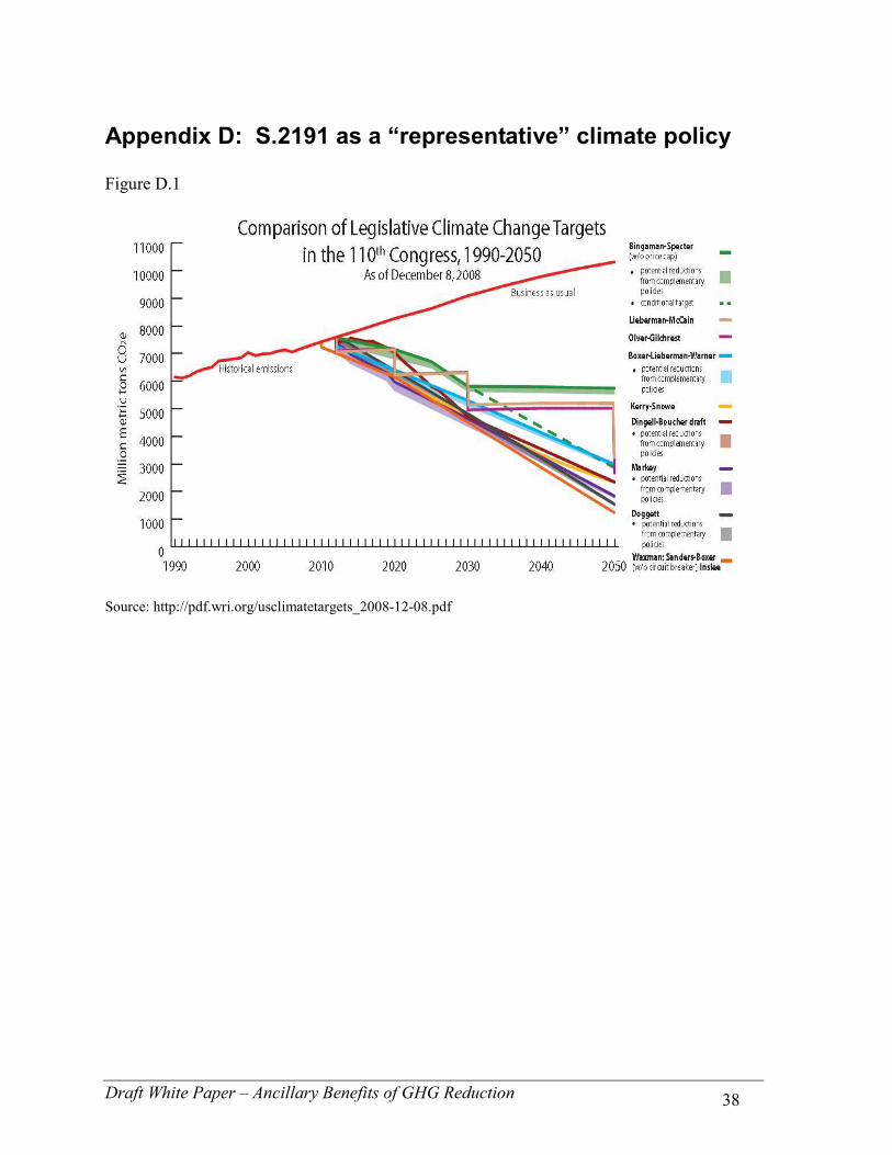
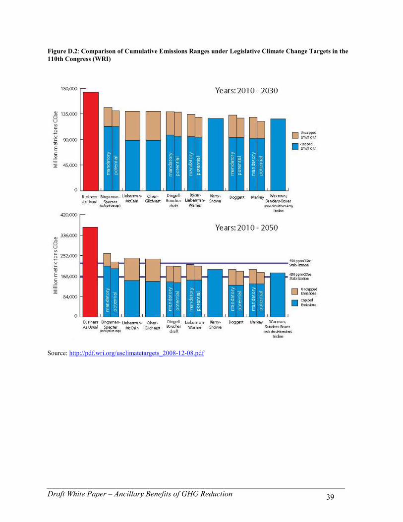
Although there are important differences among these federal cap-and-trade proposals, there are
strong similarities in the emission reduction targets and the timing of the emission reductions
among these bills (see figures D1 and D2 in Appendix D). The scenario analyzed in this paper is
that projected to occur given the enactment of S.2191. Although the analysis is specific to
S.2191, this scenario is a representative U.S. climate policy in terms of both emission reduction
targets and the timing of such reductions (see Appendix D). An additional advantage of using
S.2191 as the representative policy is that, the U.S. Environmental Protection Agency (USEPA)
provides corresponding carbon allowance prices, sectoral abatement and other projections which
are required to carry out the empirical analysis in the current paper. Specifically, in March 2008,
Draft White Paper – Ancillary Benefits of GHG Reduction 6
the USEPA released its macroeconomic analysis of the Lieberman-Warner bill from 2012 to
2050 (USEPA, 2008). The modeling apparatus in the USEPA’s study draws on the results from
two economic models: the ADAGE model and the IGEM model4 . The USEPA study is an
analysis of the costs of reducing carbon emissions over the entire duration of the program, from
2012 through 20505.
In this analysis we use the results from the ADAGE Core Scenario 2 which models the bill as
written. The reason for using the results from ADAGE is that the allowance prices estimated by
this model are towards the center of the range of allowance prices reported by IGEM and a
recent USEPA analysis of the bill currently under discussion in Congress (ACES HR2454). The
range of permit prices is shown in table C1 (Appendix C).
3 Emission Modeling
The analysis of ancillary benefits due to climate policy effectively compares emissions of SO2,
PM2.5, PM10, NOx, NH3, and VOC under two different scenarios. The first scenario projects local
pollutant emissions that reflect BAU assumptions regarding demand growth between 2006 and
2030 given current environmental policies, transportation fuel prices, and electricity prices. The
second scenario reflects emissions of local pollutants given the enactment of a federal climate
policy over the same time period as the BAU scenario. The analysis models changes in emissions
4 Both are dynamic computable general equilibrium (CGE) models The ADAGE model was developed at Research Triangle Institute (RTI) in North Carolina (see www.rti.org/adage . IGEM was developed at Harvard University (http://www.economics.harvard.edu/faculty/jorgenson/files/IGEM%20Documentation.pdf). 5 The EPA analysis is available online at http://www.epa.gov/climatechange/downloads/s2191_EPA_Analysis.pdf; the complete results are available at http://www.epa.gov/climate change/downloads/DataAnnex-S.2191.zip.
Draft White Paper – Ancillary Benefits of GHG Reduction 7
in both the electric power generation sector and the transportation sector. Emissions from other
sectors are held fixed. The APEEP model accepts emission inputs associated with each of these
two scenarios, and it estimates exposures, premature mortalities, increased rates of illness, and
monetary damage associated with both scenarios. The ancillary benefits reported in section 4
reflect the difference in damages due to emissions of SO2, PM2.5, PM10, NOx, NH3, and VOC
between the BAU and the policy scenarios.
3.1 Modeling emissions from electricity production.
As mentioned above, the results from USEPA's ADAGE Core Scenario 2 are used to represent
the impact of the Warner-Lieberman Climate bill on electric power generation. While the
USEPA model provides detailed information regarding such variables as total electric
generation, allowance prices, and CO2 emissions, it does not provide the unit level geographic
generation and emission details needed to analyze the co-benefits associated with the reduction
in other pollutants. In this study the emission reductions from specific electric generating point
sources is estimated using an electricity production-cost model. The Regional Electricity Model
(REM) is described in detail in Appendix B.
This application of the REM consists of two model runs; a BAU case and a policy case
representing the S.2191. Emission reductions are calculated by comparing projected emissions
given the two model runs. The BAU case is benchmarked to USEPA's reference case6 and the
policy case is benchmarked to the ADAGE Core Scenario 2 results for electric generation, CO2
emissions, fuel prices, allowance prices, and new capacity additions. The BAU case includes
6 This scenario served as the benchmark case to which the various ADAGE model runs were compared.

Draft White Paper – Ancillary Benefits of GHG Reduction 8
emissions reductions associated with the Clean Air Interstate Rule (CAIR)7. Further, the policy
case assumes that the CAIR emission caps remain in effect. The REM provides detailed
modeling results for all electricity generating sources in the contiguous U.S. greater than 25 MW
in size. These generating units comprise over 9,500 point sources. Annual emission data for
these 9,500 point sources are matched to APEEP in two ways. First emissions from 656
individual electric generating units modeled in APEEP are matched according to facility. The
remaining smaller sources have their emissions aggregated to the county level which are then
input to the source-receptor matrices in APEEP.
3.2 Modeling emissions from transportation.
The transportation BAU emission projections are based on USEPA’s emission inventory for the
period 2002 - 2030 (Air Quality & Modeling Center Assessment & Standards Division - U.S.
EPA Office of Transportation & Air Quality)8. The on-road emissions are based the National
Mobile Inventory Model (NMIM) using MOBILE69 emission factors. The USEPA emissions
projections account for all finalized USEPA regulations and include the Renewable Fuel
Standard (RFS1). Some emission source projections (such as aircraft) are based on the U.S. 7 The Clean Air Interstate Rule proposes a reduction in SO2 and NOx emissions in 28 Eastern states and the district of Columbia. Under CAIR, SO2 emissions would be reduced by 70 percent and NOx emissions reduced by 60 percent in the CAIR region. The CAIR is currently under litigation. See http://www.epa.gov/cair/ for more information. 8 These data are derived from the public version of USEPA's emission inventory for 2002 -2030 as provided to us by the US EPA, Office of Transportation and Air Quality. 9 The National Mobile Inventory Model (NMIM) is a computer application developed by EPA to help develop estimates of current and future emission inventories for on-road motor vehicles and non-road equipment. NMIM uses current versions of MOBILE6 and NONROAD to calculate emission inventories, based on multiple input scenarios that are entered into the system. NMIM can be used to calculate national, individual state or county inventories. Vehicle Emission Modeling Software and related presentations and training resources. MOBILE6 is an emission factor model for predicting gram per mile emissions of Hydrocarbons (HC), Carbon Monoxide (CO), Nitrogen Oxides (NOx), Carbon Dioxide (CO2), Particulate Matter (PM), and toxics from cars, trucks, and motorcycles under various conditions. NONROAD is another EPA Model. Its primary use is for estimation of air pollution inventories.
Draft White Paper – Ancillary Benefits of GHG Reduction 9
Department of Energy, Energy Information Agency’s emission forecast (USDOE, 200710) and
thus do not take into account any changes which may have occurred due to regulations which
came into force after 2007 (for example, the Energy Independence and Security Act of 2007).
The policy scenario for transport emissions of GHGs is dictated by the aggregate GHG emission
cap which is applied upstream on petroleum production; refineries and importers of
transportation fuel are directly covered under the cap. Such an upstream compliance obligation
captures the transportation sector without having to bring individual cars and trucks under a cap.
In this study, the effect of the GHG cap on transportation emissions is modeled through the price
effects on fuels, the resulting change in consumption of transportation fuels, and corresponding
change to emissions. We rely on USEPA’s estimates of fuel price increases from 2012 through
205011 . The expected price increases of fuels from the climate policy are shown in Table C2
(Appendix C). Published demand elasticities are used to estimate the reduced use of fuels that
would result given the price increases projected to occur as a result of climate policy. Table C3
shows estimates of the long-run gasoline price elasticity. Other transportation modes employ
different fuels. For diesel, compressed natural gas (CNG) and other transport fuels we rely on the
price elasticities shown in Table C4.
It is important to note that this approach produces projections which model the influence of the
climate policy on demand for existing fuels based on past evidence of price impacts. However, it
10 More specifically EIA’s AEO2007. 11 The EPA analysis is available online at http://www.epa.gov/climatechange/downloads/s2191_EPA_Analysis.pdf; the complete results are available at http://www.epa.gov/climate change/downloads/DataAnnex-S.2191.zip.
Draft White Paper – Ancillary Benefits of GHG Reduction 10
does not include a potential shift to fuels with much lower carbon content. The analysis may
therefore underestimate the pollution reductions to be expected from a climate policy if
significant substitution of fuel were to occur.
4 Modeling Air Pollution Damages
This study uses the APEEP model (Muller, Mendelsohn, 2007), which is calibrated to simulate
the consequences of both the BAU and policy scenarios. In terms of its structure, APEEP is a
traditional integrated assessment model in that it resembles integrated assessment models used
by USEPA and other researchers to measure the impacts of air pollution (Mendelsohn, 1980;
Nordhaus, 1992; USEPA, 1999). Specifically, the model begins with emissions and then it uses
an air quality model to determine where emissions travel to and the degree to which they react
with other pollutants in the atmosphere. Next APEEP computes exposures of people to ambient
air pollution. Finally, APEEP determines the resulting human health impacts and the monetary
value of such impacts. The following sections describe the key components of the APEEP model
in more detail.
The emission sources modeled in APEEP are grouped into four broad categories. First are the
ground-level emissions which include mobile sources and stationary sources without a tall
smokestack. These are further subdivided according to vehicle type, fuel type, and for stationary
sources, the different categories that the USEPA identifies in its national emission inventory:
agriculture, forestry, and mining, for example. APEEP also models point sources with three
Draft White Paper – Ancillary Benefits of GHG Reduction 11
distinct effective heights12; low stack sources (effective height less than 250 meters): including
most manufacturing facilities; medium stack sources (effective height between 250 and 500
meters); and tall stack sources (with an effective height of greater than 500 meters). The four
source categories listed above encompass all of the emissions of the six pollutants modeled by
APEEP in the contiguous U.S. as reported by the USEPA (USEPA, 2006). Emissions from each
of the first three categories are aggregated, by pollutant, to the county level. Emissions from the
tall stack sources are modeled at the facility level.
The spatial detail in APEEP’s documentation of sources is important because, unlike the effects
of greenhouse gas concentrations which are global, the health effects of the air pollutants
modeled in APEEP are relatively localized. Following the documentation of emissions, APEEP
uses an air quality model to predict seasonal and annual average county concentrations for PM2.5,
PM10, VOC, NOx, SO2, NH3 and tropospheric ozone (O3). The air quality model simulates
transport, chemical transformation into other pollutants, and deposition of each emitted species.
This model is discussed in Muller, Mendelsohn (2007). Note that APEEP takes atmospheric
chemistry into account. This is important because, following emission, some of the pollutants
tracked by the model transform in the atmosphere into more harmful pollutants; for example,
SO2 emissions become particulate sulfate and NOx emissions contribute to concentrations of both
particulate nitrate and O3. The damages from these secondary pollutants are attributed to the
sources that produced the emission.
APEEP then calculates human exposures to the predicted concentrations by multiplying county-
level pollution concentrations by the county-level population data. Current population levels are 12 Effective height is defined as stack height plus eventual plume rise.
Draft White Paper – Ancillary Benefits of GHG Reduction 12
provided by the U.S. Department of the Census while future population projections are provided
by the Center for Disease Control. In the APEEP model, populations are differentiated by age
because the health impacts of local air pollution are proportional to baseline incidence rates
which are age-dependent.
APEEP translates exposures into physical effects using concentration-response functions
published in peer-reviewed studies in the epidemiological literature. The full list of
concentration-response functions used in APEEP is found in Muller and Mendelsohn (2007).
Because premature mortalities account for the vast majority of damages due to exposures to the
local air pollutant, we focus here on the concentration-response functions that govern the
relationship between the annual mean level of PM2.5 and adult mortality rates, infant mortality
rates, as well as the relationship between exposures to O3 and all age mortality rates. To model
the relationship between PM2.5 exposures and adult mortality rates APEEP employs the results
from Pope et al., (2002). The relationship between infant mortality rates and exposure to PM2.5 is
captured using the findings in Woodruff et al., (2006). Finally, the results from Bell et al. (2004)
govern the impact of O3 exposure on mortality rates of all ages. APEEP also measures the
damages due to chronic illnesses such as chronic bronchitis and asthma in addition to mortality
(Abbey et al. 1999; McDonnell, 1999).
APEEP expresses the value of the physical effects resulting from exposures to air pollution in
dollar terms13. Applying monetary values to effects on human health, especially premature
mortalities is methodologically difficult and politically controversial. The published literature
relies upon two approaches to value premature mortality risks: revealed preference and stated 13 Note that all values are expressed in constant year 2006 U.S. dollars.
Draft White Paper – Ancillary Benefits of GHG Reduction 13
preference methods (Cropper, Oates, 1992; Viscusi, Aldy, 2003) For mortality valuation, APEEP
uses the results from a meta-analysis that encompasses both the revealed preference literature
that uses hedonic wage models to estimate the relationship between wages and occupation-
specific mortality rates and the stated preference literature which asks people what they would be
willing to pay to avoid mortality risks on surveys (USEPA, 1999). The literature notes that
dividing the risk premium (R), which reflects how much workers require in extra pay in order to
assume an additional, incremental risk of death, by the change in the probability of death (∆γ)
yields the value of a statistical life (VSL) , (Viscusi, Aldy, 2003).
VSL=(R/∆γ) (1)
One complication in the application of VSLs is whether this parameter should be applied
uniformly to people of all ages or whether the VSL should be differentiated by age. This is
important because the estimates of VSL are derived from studies that focus on working age
people but most of the mortalities from air pollution affect the elderly and the very young. This
study adopts the approach employed by the USEPA and other federal agencies which apply the
VSL uniformly to populations of all ages (USEPA, 1999).
In addition to the baseline scenario, we conduct a sensitivity analysis in order to test the
importance of specific assumptions in the model to the benefit estimates for emission reductions.
Because the literature indicates that health damages comprise the largest share of air pollution
damages the sensitivity analysis focuses on alternative ways to model health effects (USEPA,
1999; Muller, Mendelsohn, 2007). In the first alternative scenario we employ an alternative
Draft White Paper – Ancillary Benefits of GHG Reduction 14
concentration-response function relating long-term PM2.5 exposures to adult mortality rates using
the results from Laden et al., (2006). Second, because the study extends far into the future we
alter the assumptions regarding rates of personal income growth over the period 2006-2030. The
default case employs the rate of growth used in the ADAGE model (3.0% annual growth). In our
alternative scenarios, we employ 2.7% as an alternative rate of income growth which is
employed in IGEM. Finally, in each case we use the USEPA’s reported value for the elasticity
between income and willingness to pay to avoid mortality risk: 0.5. This is employed to adjust
the VSL in future years. Finally, APEEP discounts all future benefits to their present value at a
5% discount rate.
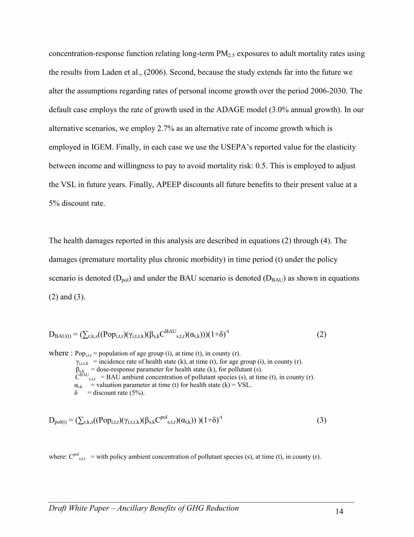
The health damages reported in this analysis are described in equations (2) through (4). The
damages (premature mortality plus chronic morbidity) in time period (t) under the policy
scenario is denoted (Dpol) and under the BAU scenario is denoted (DBAU) as shown in equations
(2) and (3).
DBAU(t) = (∑r,k,s((Popi,t,r)(γi,t,r,k)(βs,kCBAUs,t,r)(αt,k)))(1+δ)-t (2)
where : Popi,t,r = population of age group (i), at time (t), in county (r). γi,t,r,k = incidence rate of health state (k), at time (t), for age group (i), in county (r). βs,k = dose-response parameter for health state (k), for pollutant (s). CBAU
s,t,r = BAU ambient concentration of pollutant species (s), at time (t), in county (r). αt,k = valuation parameter at time (t) for health state (k) = VSL. δ = discount rate (5%).
Dpol(t) = (∑r,k,s((Popi,t,r)(γi,t,r,k)(βs,kCpols,t,r)(αt,k)) )(1+δ)-t (3)
where: Cpols,t,r = with policy ambient concentration of pollutant species (s), at time (t), in county (r).
Draft White Paper – Ancillary Benefits of GHG Reduction 15
The co-benefits of climate policy in any one time period (t) is the difference in damages between
the policy (Dpol) and the BAU (DBAU) scenarios. The total benefits are the discounted sum of the
difference between BAU and policy damages over (t) as shown in (4).
D = ∑t(DBAU(t) – Dpol(t)) (4)
As this study has focused solely on the health benefits it is a de facto underestimate of the actual
total ancillary benefits. Some examples of the benefits this study does not capture include:
reduced yields of agricultural crops and timber due to tropospheric ozone (O3), reductions in
visibility from reduced emission of fine particles (PM10, PM2 and SO2), enhanced depreciation
of man-made materials (buildings and historical monuments) from acid rain contributed to by
emission of NOx and SO2; and damages due to lost recreation services (deterioration of water
quality in recreational fishing areas). Muller and Mendelsohn (2007) found that human health
impacts accounted for over 90% of the total damages from the local air pollutants modeled in
APEEP.
5 Results
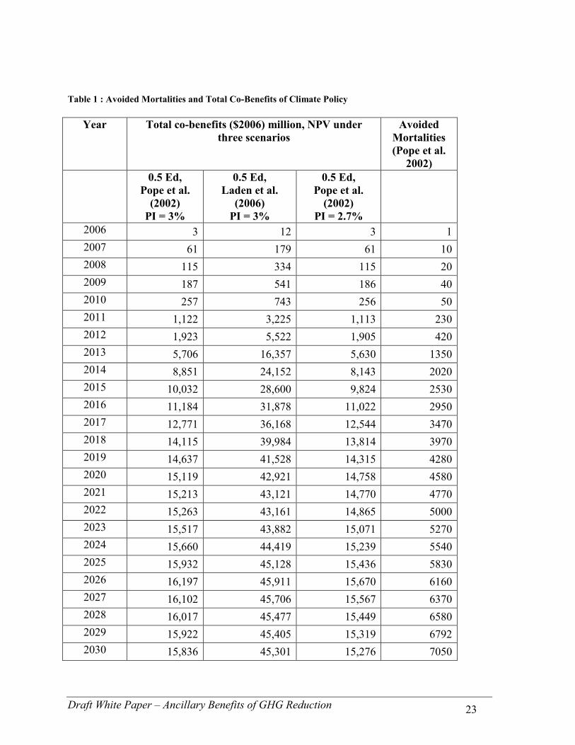
Table 1 displays the principal results of this study. These include both the estimated premature
mortalities using the default assumptions in the APEEP model as well as the annual co-benefits
of climate policy from 2006 until 2030 for each of the three modeling scenarios. Since climate
policy begins with modest reductions in GHGs, the emission reductions of local pollutants are
also relatively small in the early years of this analysis. As a result, both the co-benefits and the
projected avoided mortalities begin low and increase as the climate policy becomes more
stringent.
Draft White Paper – Ancillary Benefits of GHG Reduction 16
The right-hand column in Table 1 indicates the premature mortalities avoided begin at 1 case in
2006 and then increase to greater than 200 in 2011. The number of avoided deaths continues to
grow to just less than 5,000 in 2020 and finally rises to over 7,000 avoided deaths in 2030.
Table 1 also reports the aggregate ancillary benefits of the GHG abatement policy. The results
are broken down by year in order to show the relative magnitudes of the benefits generated over
the 25 year time period covered in this paper. The benefits are expressed in present value terms
(discounted at 5%). The first column (second from the left) corresponds to the default scenario,
with the dose-response function relating adult mortality rates to exposures to PM2.5 derived from
Pope et al., (2002), personal income growth of 3%, and the elasticity between willingness-to-pay
to avoid mortality risks and income of 0.5.
The first pattern of note is that the estimated co-benefits generally increase from the first year of
the policy through 2026. This occurs for three reasons. First, greater amounts of GHGs are
abated (as the aggregate cap on emissions becomes tighter). This implies that increasing amounts
of local pollutants are abated as well. Second, populations grow between 2006 and 2030; as a
result the population potentially exposed to local air pollutants increases as well. Hence, for a
given reduction in emissions, the health-related benefits of such reductions will increase with
greater populations. These first two factors are reflected in the increasing number of avoided
mortalities reported in Table 1. That is, greater reductions in harmful emissions and larger
exposed populations translates into more avoided deaths. The final factor that has an influence
on the increasing co-benefits through time is the following; as income grows, the value attributed
Draft White Paper – Ancillary Benefits of GHG Reduction 17
to avoided mortality risk becomes larger, too. Therefore, each avoided mortality is attributed a
larger value because the willingness-to-pay to avoid mortality risks is an increasing function of
personal income.
With the default scenario, benefits begin at $3 million in 2006, and increase to $16.2 billion in
2026. Thereafter, benefits decline to $15.8 billion in 2030. Benefits decline in the distant future
because of discounting. Hence, although the projected number of avoided mortalities grows
steadily from 2006 through 2030, the co-benefits begin to decline in 2027 due to discounting.
The total benefit of climate change policy in the default case is $254 billion, in present value
terms. For the two alternative scenarios the pattern in benefits accrued through 2030 is quite
similar to the default case; benefits begin at modest levels and then they increase through 2026
and then begin to decline in 2027 through 2030. However, the magnitudes of the co-benefits are
considerably larger in the second scenario (shown in the third column from the left). Recall that
this perturbation employs an alternative dose-response function corresponding to the adult
mortality-PM2.5 relationship (see Laden, et al., 2006). In particular, the dose-response parameter
reported in the Laden et al. (2006) study is nearly three times larger than the parameter reported
in the Pope et al. (2002) study.
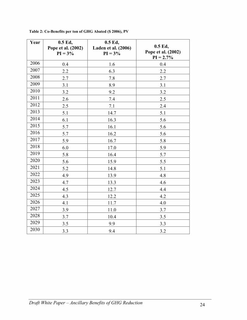
Table 2 provides an alternative perspective on the benefits of climate change policy. This table
expresses the co-benefits in terms of per ton of GHG abated for each year in the analysis. In the
default scenario, benefits per ton of GHG (CO2e) begin at $0.40 in 2006, and then increase to
$6.0 in 2018. Thereafter, per ton benefits decline to $3.30 in 2030. The results shown in this
Draft White Paper – Ancillary Benefits of GHG Reduction 18
table are especially powerful when viewed in conjunction with recent estimates of the marginal
abatement costs for GHGs. Specifically, USEPA finds that the inter-temporal average present
value marginal abatement costs are projected to be $9/ton CO2e (USEPA, 2008).
As with Table 1, the inter-temporal pattern in benefits per ton of abatement are similar across the
three scenarios while the magnitudes are quite different for the second scenario. That is, the
benefits per ton of GHG are nearly three-times larger when using the alternate dose-response
function. Notably, benefits per ton increase to $17/ton CO2e in 2018.
Another interesting pattern is evident in Table 2. Benefits per ton of GHG increase from 2006
until 2010, then per ton benefits decline in 2011 and 2012 and begin to increase again in 2013.
This occurs because the emission reductions in the transportation sector begin in 2011, which
drives down the benefit per ton of CO2e.
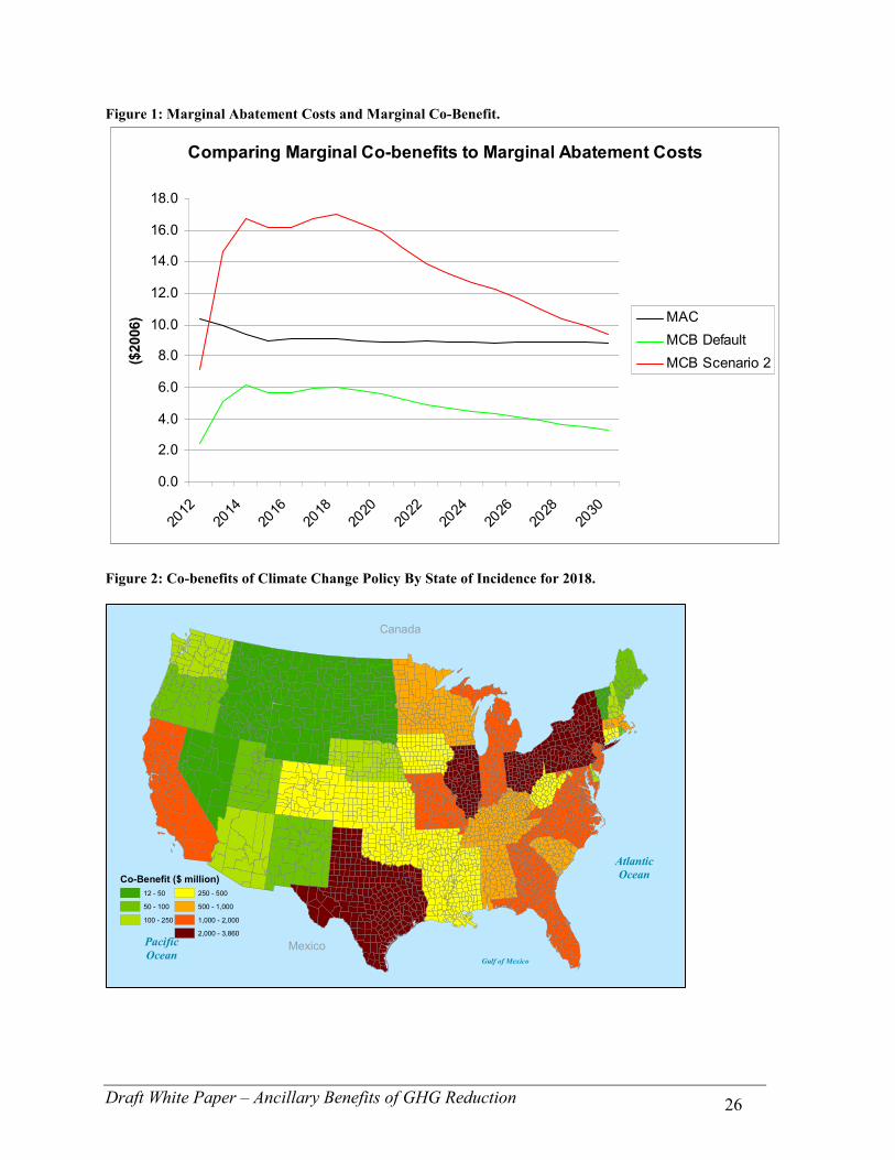
Figure 1 provides a comparison of the present value of marginal co-benefits per ton CO2e with
the marginal abatement costs. The figure includes the marginal co-benefits estimated with
APEEP modeling scenario 1 and 2. With scenario 1, marginal co-benefits average $5 per ton
CO2e over the period from 2012 – 2030. Under modeling scenario 2, the average co-benefit is
nearly $14 per ton CO2e. Over the same time period, marginal abatement costs average $9. This
implies that the estimated marginal co-benefit for abatement of GHG is comparable to the
marginal abatement cost without including direct benefits of climate stabilization. Because the
co-benefits reported in this paper nearly balance the costs of abatement at the margin, the
argument for aggressive abatement of GHGs is significantly strengthened.
Draft White Paper – Ancillary Benefits of GHG Reduction 19
Figure 2 displays the spatial distribution of benefits from climate change policy in the year 2018.
In general, the aggregate benefits occur in states with large populations. New York,
Pennsylvania, Ohio, Illinois, and Texas all are projected to incur co-benefits of greater than $2
billion in the year 2018. It is interesting to note that California, which has the largest state
population, is not in the highest benefit category. This is the case for two reasons. First, with
prevailing winds from the west, California does not have any emission sources of local pollutants
directly upwind. Second, much of California’s energy is produced with natural gas and much of
the aggregate co-benefits in other states are due to the reduced use of coal in energy production.
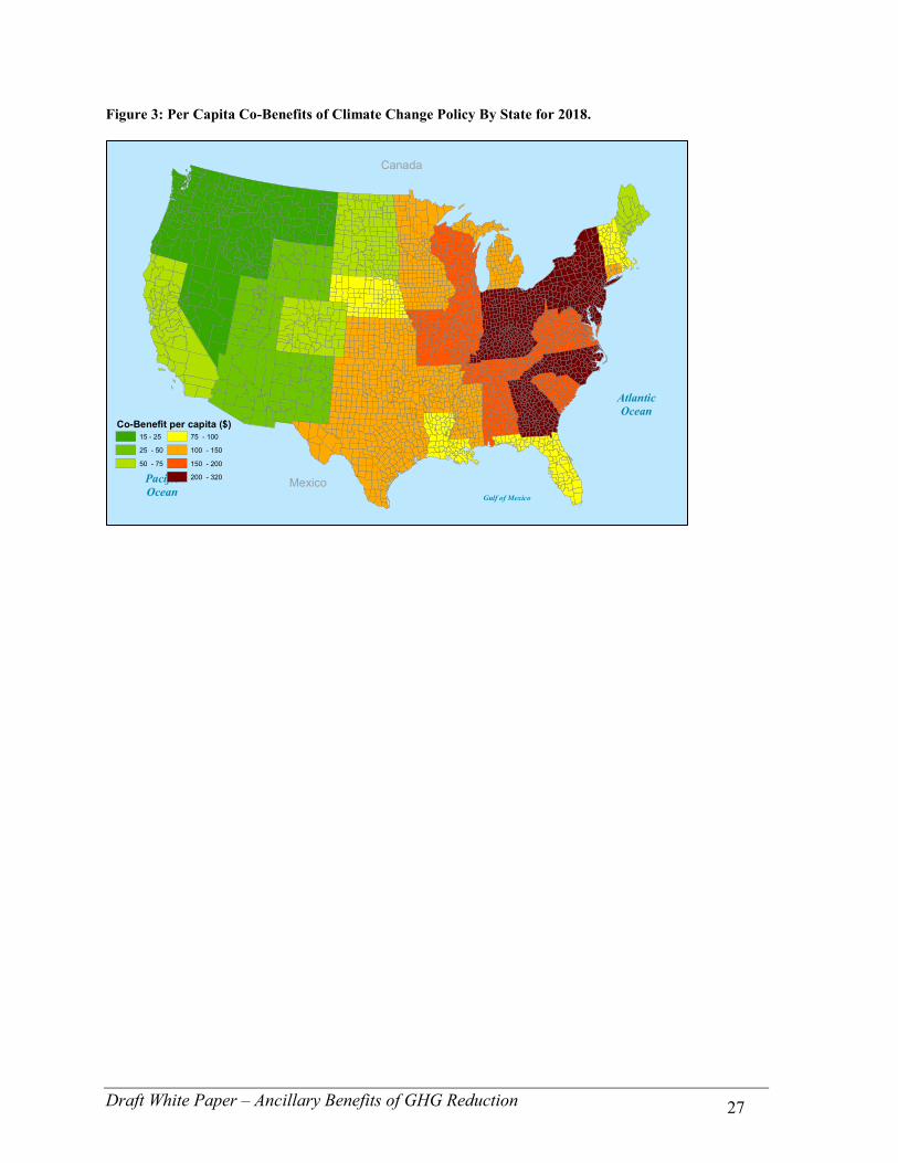
Figure 3 displays the per capita co-benefits by state. The spatial pattern in Figure 2 is striking; all
of the states that are projected to experience the largest per capita co-benefits of climate change
policy are located east of the Mississippi River. These include: Indiana, Ohio, Kentucky,
Pennsylvania, Maryland, New York, Delaware, New Jersey, Georgia, and North Carolina. This
figure emphasizes the importance of coal to the overall co-benefits analysis. That is, much of the
total co-benefits estimated to occur as a result of this climate change policy stem from a
reduction in the amount of coal burned to produce electricity. Since, most of the coal-fired
electric power generation capacity is located in the Southeast and the Midwest, the benefits due
to burning less coal will accrue in areas proximal to these generators and areas downwind (to the
east).
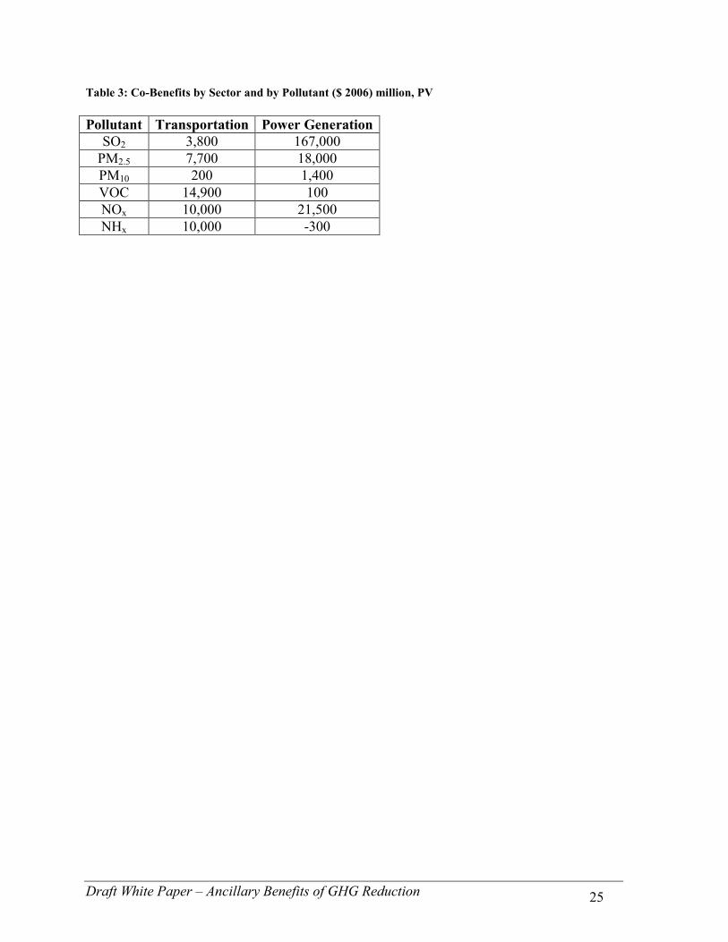
Table 3 provides a detailed decomposition of the total co-benefits by pollutant and by sector.
First, Table 3 indicates that of the $254 billion total co-benefits that are projected to occur (under
Draft White Paper – Ancillary Benefits of GHG Reduction 20
the default modeling scenario) $208 billion are a result of emission reductions in the electric
power generation sector. This implies that $47 billion worth of the co-benefits stem from
abatement in the transportation sector. With the electric power generation sector, SO2 reductions
account for the largest share of benefits: $167 billion of the $208 total. This is due to burning
less coal in order to generate electricity. This result reinforces the pattern evident in figure 2;
most of the co-benefits occur in the eastern U.S. where coal is the predominant fuel used to
generate power.
The next largest share of benefits within the power generation sector is due to abatement of NOx;
benefits attributable to NOx abatement are worth $21.5 billion. Finally, abatement of fine
particulate matter (PM2.5) generates benefits of $18 billion. Within the transportation sector,
reduced emissions of VOC yield benefits of nearly $15 billion. Abatement of NOx and NH3 each
produce benefits of $10 billion. Reduced emissions of PM2.5 correspond to benefits of nearly $8
billion.
6 Conclusions and policy recommendations
This analysis provides strong evidence that climate change policy in the U.S. will generate
significant returns to society in addition to the returns due to climate stabilization. Aside from the
benefits stemming directly from reduced GHG emissions, the health-related co-benefits
associated with a representative climate policy range between $254 and $720 billion, in present
value terms, depending on modeling assumptions. These co-benefits are due to improvements in
health status associated with projected emissions reductions of SO2, PM2.5, PM10, NOx, NH3, and
VOC. Since the co-benefits estimated in this paper do not account for the manufacturing sector,
Draft White Paper – Ancillary Benefits of GHG Reduction 21
the co-benefits stemming from federal climate policy in the U.S. are likely to be larger than what
is reported herein.
The analysis finds that the co-benefits of climate change policy are not uniformly distributed
across the U.S. Total co-benefits are clustered in the states with the largest populations. This is
intuitive given that the benefits modeled in this study concentrate on human health impacts.
However, in per capita terms the co-benefits display a far more interesting pattern. Specifically,
the states that are projected to enjoy the greatest per capita co-benefits are all east of the
Mississippi River. The reason for this striking spatial pattern is that the majority of the co-
benefits are projected to be due to reduced reliance on coal in electric power generation. Much of
the existing generation capacity located in the Midwestern and eastern U.S. uses coal. As climate
change policy creates incentives to move away from coal towards natural gas and renewables,
the health-related benefits of this shift are likely to occur in states nearby and downwind of the
large existing coal-fired power plants. In fact, nearly two-thirds of the total projected co-benefits
stem from reduced SO2 emissions from electric power generators. Much of this SO2 abatement is
a result of moving away from the use of coal to generate electric power.
On a per ton GHG basis, these co-benefits over the time period 2012 - 2030 are estimated to
average between $5 and $14. USEPA estimates for total abatement costs permit an estimation
of14 the marginal abatement cost for a ton of CO2e. Over the period 2012 to 2030, the marginal
abatement costs are predicted to average $9. This implies that the estimated marginal co-benefit
14See slide 74 of the, EPA Analysis of the Lieberman-Warner Climate Security Act of 2008, S. 2191 in 110th Congress, March 14, 2008. The abatement from the electricity sector for the Adage scenario 2 model run was provided to us by the RTI modeling group. The abatement from the transport sector was estimated to be proportional to the forecast reductions in petroleum use for this same model run
Draft White Paper – Ancillary Benefits of GHG Reduction 22
for abatement of GHG is worth between 55 and 150 percent of the marginal abatement cost
without including direct benefits of climate stabilization. Because the co-benefits reported in this
paper nearly balance the costs of abatement at the margin, this analysis strengthens the argument
for aggressive abatement of GHGs in the U.S.
Draft White Paper – Ancillary Benefits of GHG Reduction 23
Table 1 : Avoided Mortalities and Total Co-Benefits of Climate Policy
Year Total co-benefits ($2006) million, NPV under
three scenarios Avoided
Mortalities (Pope et al.
2002) 0.5 Ed,
Pope et al. (2002) PI = 3%
0.5 Ed, Laden et al.
(2006) PI = 3%
0.5 Ed, Pope et al. (2002)
PI = 2.7%
2006 3 12 3 1 2007 61 179 61 10 2008 115 334 115 20 2009 187 541 186 40 2010 257 743 256 50 2011 1,122 3,225 1,113 230 2012 1,923 5,522 1,905 420 2013 5,706 16,357 5,630 1350 2014 8,851 24,152 8,143 2020 2015 10,032 28,600 9,824 2530 2016 11,184 31,878 11,022 2950 2017 12,771 36,168 12,544 3470 2018 14,115 39,984 13,814 3970 2019 14,637 41,528 14,315 4280 2020 15,119 42,921 14,758 4580 2021 15,213 43,121 14,770 4770 2022 15,263 43,161 14,865 5000 2023 15,517 43,882 15,071 5270 2024 15,660 44,419 15,239 5540 2025 15,932 45,128 15,436 5830 2026 16,197 45,911 15,670 6160 2027 16,102 45,706 15,567 6370 2028 16,017 45,477 15,449 6580 2029 15,922 45,405 15,319 6792 2030 15,836 45,301 15,276 7050
Draft White Paper – Ancillary Benefits of GHG Reduction 24
Table 2: Co-Benefits per ton of GHG Abated ($ 2006), PV
Year 0.5 Ed, Pope et al. (2002)
PI = 3%
0.5 Ed, Laden et al. (2006)
PI = 3% 0.5 Ed,
Pope et al. (2002) PI = 2.7%
2006 0.4 1.6 0.4 2007 2.2 6.3 2.2 2008 2.7 7.8 2.7 2009 3.1 8.9 3.1 2010 3.2 9.2 3.2 2011 2.6 7.4 2.5 2012 2.5 7.1 2.4 2013 5.1 14.7 5.1 2014 6.1 16.3 5.6 2015 5.7 16.1 5.6 2016 5.7 16.2 5.6 2017 5.9 16.7 5.8 2018 6.0 17.0 5.9 2019 5.8 16.4 5.7 2020 5.6 15.9 5.5 2021 5.2 14.8 5.1 2022 4.9 13.9 4.8 2023 4.7 13.3 4.6 2024 4.5 12.7 4.4 2025 4.3 12.2 4.2 2026 4.1 11.7 4.0 2027 3.9 11.0 3.7 2028 3.7 10.4 3.5 2029 3.5 9.9 3.3 2030 3.3 9.4 3.2
Draft White Paper – Ancillary Benefits of GHG Reduction 25
Table 3: Co-Benefits by Sector and by Pollutant ($ 2006) million, PV Pollutant Transportation Power Generation
SO2 3,800 167,000 PM2.5 7,700 18,000 PM10 200 1,400 VOC 14,900 100 NOx 10,000 21,500 NHx 10,000 -300
Draft White Paper – Ancillary Benefits of GHG Reduction 26
Figure 1: Marginal Abatement Costs and Marginal Co-Benefit.
Comparing Marginal Co-benefits to Marginal Abatement Costs
0.0
2.0
4.0
6.0
8.0
10.0
12.0
14.0
16.0
18.0
2012
2014
2016
2018
2020
2022
2024
2026
2028
2030
($2006) MAC
MCB Default
MCB Scenario 2
Figure 2: Co-benefits of Climate Change Policy By State of Incidence for 2018.
Gulf of Mexico
AtlanticOcean
PacificOcean
Canada
Mexico
Co-Benefit ($ million)12 - 50
50 - 100
100 - 250
250 - 500
500 - 1,000
1,000 - 2,000
2,000 - 3,860
Draft White Paper – Ancillary Benefits of GHG Reduction 27
Figure 3: Per Capita Co-Benefits of Climate Change Policy By State for 2018.
Gulf of Mexico
AtlanticOcean
PacificOcean
Canada
Mexico
Co-Benefit per capita ($)15 - 25
25 - 50
50 - 75
75 - 100
100 - 150
150 - 200
200 - 320

Draft White Paper – Ancillary Benefits of GHG Reduction 28
References Bell, Michelle L., Adrian McDermott, Scott L. Zeger, Jonathan M. Samet, and Francesca Domenici. "Ozone and Short-Term Mortality in 95 US Urban Communities, 1987-2000." Journal of the American Medical Association, 292(19):2372-2378. 2004. Brons M, Nijkamp P, Pels E, and Rietveld P. A meta-analysis of the price elasticity of gasoline demand. A SUR approach. Energy economics. 2105-2122, Volume 30, Issue 5, 2008. Cropper, M.L., W.E. Oates. Environmental Economics: A Survey. Journal of Economic Literature. 30(2): 675-740. 1992. Espey M, Gasoline demand revisited: an international meta-analysis of elasticities. Energy Economics. 273-295, Volume 20, Issue 3, 1998. Goodwin P, Dargay J and Hanly M. Elasticities of Road Traffic and Fuel Consumption with Respect to Price and Income: A Review. Transport Reviews. 275 – 292, Volume 24, Number 3, 2004. Graham D and Glaister S. The demand for automobile fuel: a survey of elasticities. Journal of Transport Economics and Policy. 36(1): 1-25, 2002. Hagler, B. Potential for fuel taxes to reduce greenhouse gas emissions in transportation, Fuel tax policies report, prepared for the Department of Public Works and Government Services, Science Directorate, Science, Informatics and Professional Services Sector, Canada, June 1999. Hughes J, Knittel C, and Sperling D. Evidence of a Shift in the Short-Run Price Elasticity of Gasoline Demand. Center for the Study of Energy Markets. Paper CSEMWP-159. 2007. F. Laden, J. Schwartz, F.E. Speizer, D.W. Dockery. Reduction in Fine Particulate Air Pollution and Mortality: Extended Follow-up of the Harvard Six Cities Study, Amer. J. of Respiratory and CriticalCare Medicine, 173: 667-672. 2006. Muller, N.Z., R.O. Mendelsohn,. Measuring the Damages of Air Pollution in the United States. Journal of Environmental Economics and Management. 54(1):1-14. 2007 Nicol, C. Elasticity of Demand for Gasoline in Canada and the United States. Department of Economics, University of Regina. 2000. Puller S., L. Greening. Household adjustment to gasoline price change: an analysis using 9 years of US survey data. Energy Economics. 37-52, Volume 21, Issue 1, 1999. Romero A. Revisiting the Price Elasticity of Gasoline Demand. Department of Economics, College of William and Mary. Working paper 63. 2006.
Draft White Paper – Ancillary Benefits of GHG Reduction 29
Small, K. K. Van Dender, Fuel Efficiency and Motor Vehicle Travel: The Declining Rebound Effect. The Energy Journal. 25-51, Volume 28, Number 1, 2007. U.S. Department of Energy, (USDOE) 2007. http://tonto.eia.doe.gov/ftproot/forecasting/0383(2007).pdf U.S. Environmental Protection Agency (USEPA). The Benefits and Costs of the Clean Air Act: 1990 - 2010. EPA Report to Congress. EPA 410-R-99-001, Washington, DC, Office of Air and Radiation, Office of Policy. 1999. U.S. Environmental Protection Agency (USEPA). National Emissions Inventory (NEI): 2002. Washington, DC: Office of Air Quality Planning and Standards, Emissions Inventory Group; Emissions, Monitoring, and Analysis Division. 2006. U.S. Environmental Protection Agency (USEPA), Office of Atmospheric Programs, EPA Analysis of the Lieberman-Warner Climate Security Act of 2008, S. 2191 in 110th Congress, March 14, 2008. U.S. Environmental Protection Agency (USEPA) Inventory of US Greenhouse Gas emissions and Sinks: 1990 – 2007, EPA 430-R-09-004, April 15, 2009. Victoria Transport Policy Institute (VTPI), Online TDM Encyclopedia, British Columbia, http://www.vtpi.org/tdm/, Updated May 2009. Viscusi, W. Kip and Joseph E. Aldy. "The Value of a Statistical Life: A Critical Review of Market Estimates Throughout the World." Journal of Risk and Uncertainty, 27(1): 5-76. 2003. Woodruff, Tracey J., Jennifer D. Parker, and Kenneth C. Schoendorf. "Fine Particulate Matter (PM2:5) Air Pollution and Selected Causes of Postneonatal Infant Mortality in California" Environmental Health Perspectives, 114(5):786-790. 2006.
Draft White Paper – Ancillary Benefits of GHG Reduction 30
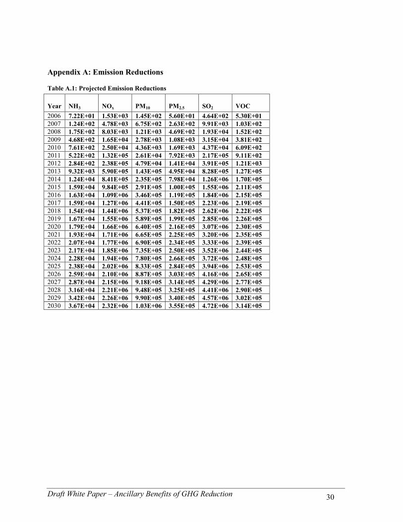
Appendix A: Emission Reductions
Table A.1: Projected Emission Reductions
Year NH3 NOx PM10 PM2.5 SO2 VOC 2006 7.22E+01 1.53E+03 1.45E+02 5.60E+01 4.64E+02 5.30E+01 2007 1.24E+02 4.78E+03 6.75E+02 2.63E+02 9.91E+03 1.03E+02 2008 1.75E+02 8.03E+03 1.21E+03 4.69E+02 1.93E+04 1.52E+02 2009 4.68E+02 1.65E+04 2.78E+03 1.08E+03 3.15E+04 3.81E+02 2010 7.61E+02 2.50E+04 4.36E+03 1.69E+03 4.37E+04 6.09E+02 2011 5.22E+02 1.32E+05 2.61E+04 7.92E+03 2.17E+05 9.11E+02 2012 2.84E+02 2.38E+05 4.79E+04 1.41E+04 3.91E+05 1.21E+03 2013 9.32E+03 5.90E+05 1.43E+05 4.95E+04 8.28E+05 1.27E+05 2014 1.24E+04 8.41E+05 2.35E+05 7.98E+04 1.26E+06 1.70E+05 2015 1.59E+04 9.84E+05 2.91E+05 1.00E+05 1.55E+06 2.11E+05 2016 1.63E+04 1.09E+06 3.46E+05 1.19E+05 1.84E+06 2.15E+05 2017 1.59E+04 1.27E+06 4.41E+05 1.50E+05 2.23E+06 2.19E+05 2018 1.54E+04 1.44E+06 5.37E+05 1.82E+05 2.62E+06 2.22E+05 2019 1.67E+04 1.55E+06 5.89E+05 1.99E+05 2.85E+06 2.26E+05 2020 1.79E+04 1.66E+06 6.40E+05 2.16E+05 3.07E+06 2.30E+05 2021 1.93E+04 1.71E+06 6.65E+05 2.25E+05 3.20E+06 2.35E+05 2022 2.07E+04 1.77E+06 6.90E+05 2.34E+05 3.33E+06 2.39E+05 2023 2.17E+04 1.85E+06 7.35E+05 2.50E+05 3.52E+06 2.44E+05 2024 2.28E+04 1.94E+06 7.80E+05 2.66E+05 3.72E+06 2.48E+05 2025 2.38E+04 2.02E+06 8.33E+05 2.84E+05 3.94E+06 2.53E+05 2026 2.59E+04 2.10E+06 8.87E+05 3.03E+05 4.16E+06 2.65E+05 2027 2.87E+04 2.15E+06 9.18E+05 3.14E+05 4.29E+06 2.77E+05 2028 3.16E+04 2.21E+06 9.48E+05 3.25E+05 4.41E+06 2.90E+05 2029 3.42E+04 2.26E+06 9.90E+05 3.40E+05 4.57E+06 3.02E+05 2030 3.67E+04 2.32E+06 1.03E+06 3.55E+05 4.72E+06 3.14E+05
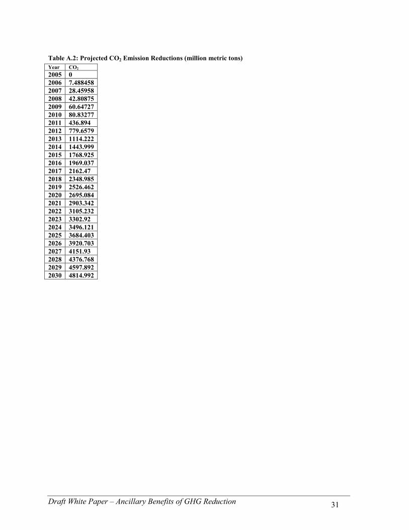
Draft White Paper – Ancillary Benefits of GHG Reduction 31
Table A.2: Projected CO2 Emission Reductions (million metric tons) Year CO2 2005 0 2006 7.488458 2007 28.45958 2008 42.80875 2009 60.64727 2010 80.83277 2011 436.894 2012 779.6579 2013 1114.222 2014 1443.999 2015 1768.925 2016 1969.037 2017 2162.47 2018 2348.985 2019 2526.462 2020 2695.084 2021 2903.342 2022 3105.232 2023 3302.92 2024 3496.121 2025 3684.403 2026 3920.703 2027 4151.93 2028 4376.768 2029 4597.892 2030 4814.992
Draft White Paper – Ancillary Benefits of GHG Reduction 32
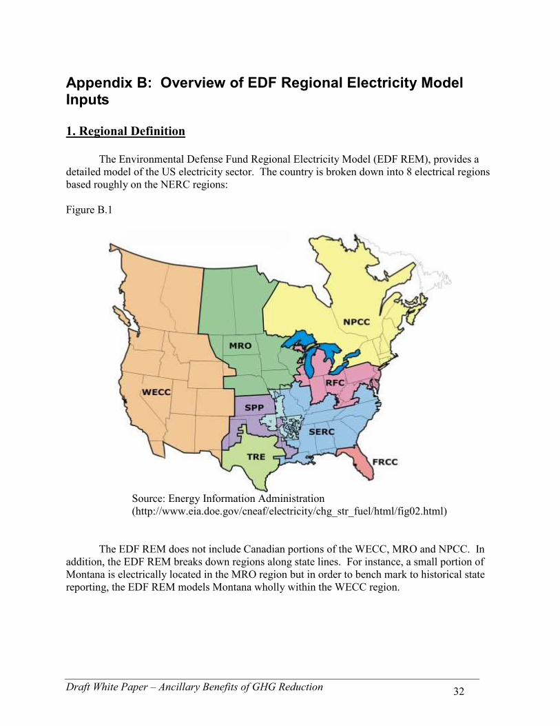
Appendix B: Overview of EDF Regional Electricity Model Inputs 1. Regional Definition The Environmental Defense Fund Regional Electricity Model (EDF REM), provides a detailed model of the US electricity sector. The country is broken down into 8 electrical regions based roughly on the NERC regions: Figure B.1
Source: Energy Information Administration (http://www.eia.doe.gov/cneaf/electricity/chg_str_fuel/html/fig02.html) The EDF REM does not include Canadian portions of the WECC, MRO and NPCC. In addition, the EDF REM breaks down regions along state lines. For instance, a small portion of Montana is electrically located in the MRO region but in order to bench mark to historical state reporting, the EDF REM models Montana wholly within the WECC region.
Draft White Paper – Ancillary Benefits of GHG Reduction 33
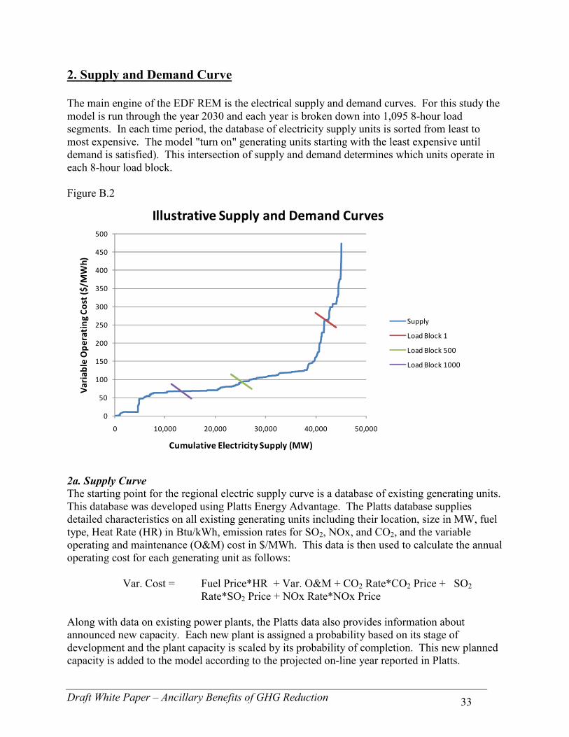
2. Supply and Demand Curve The main engine of the EDF REM is the electrical supply and demand curves. For this study the model is run through the year 2030 and each year is broken down into 1,095 8-hour load segments. In each time period, the database of electricity supply units is sorted from least to most expensive. The model "turn on" generating units starting with the least expensive until demand is satisfied). This intersection of supply and demand determines which units operate in each 8-hour load block. Figure B.2
0
50
100
150
200
250
300
350
400
450
500
0 10,000 20,000 30,000 40,000 50,000
Vari
able
Ope
rati
ng C
ost (
$/M
Wh)
Cumulative Electricity Supply (MW)
Illustrative Supply and Demand Curves
Supply
Load Block 1
Load Block 500
Load Block 1000
2a. Supply Curve The starting point for the regional electric supply curve is a database of existing generating units. This database was developed using Platts Energy Advantage. The Platts database supplies detailed characteristics on all existing generating units including their location, size in MW, fuel type, Heat Rate (HR) in Btu/kWh, emission rates for SO2, NOx, and CO2, and the variable operating and maintenance (O&M) cost in $/MWh. This data is then used to calculate the annual operating cost for each generating unit as follows: Var. Cost = Fuel Price*HR + Var. O&M + CO2 Rate*CO2 Price + SO2
Rate*SO2 Price + NOx Rate*NOx Price Along with data on existing power plants, the Platts data also provides information about announced new capacity. Each new plant is assigned a probability based on its stage of development and the plant capacity is scaled by its probability of completion. This new planned capacity is added to the model according to the projected on-line year reported in Platts.
Draft White Paper – Ancillary Benefits of GHG Reduction 34
Plant emission rates for VOCs, NH3, PM 2.5 and PM 10 are based on the EPA published emission factors by plant fuel type and firing type15. 2b. Demand Curve The starting point for the electricity demand curve is the total annual energy demanded in each region. The forecast for the annual energy demand is based on the NERC Report "2008-2017 Regional and National Peak Demand and Energy Forecasts Bandwidths." This report details the expected demand growth by NERC region. The total annual demand is broken down into 1,095 8-hour load blocks in order to represent the variation in demand across time within a given year. The hourly demand curve is developed from the EPA IPM regional load curves: "Appendix 2-1. Load Duration Curves used in Base Case 2006". This curve of 8,760 hours per year is aggregated into 8-hour blocks such that block 1 contains the highest 8 demand hours of the year and block 1,095 has the 9 lowest demand hours. These demand blocks are scaled each year to reflect the annual demand growth. 3. Fuel and Emissions Price Forecasts Fuel and emission price forecast are derived from a number of differing sources. Coal Price Platts Energy Advantage provides plant specific coal-price forecasts. The coal price for new announced coal plants with a specific site location are tied to the price forecast for the nearest existing coal plant. A weighted average coal price is developed by region for use in new economic coal plant additions. Natural Gas and Oil Price The natural gas price forecast is based on the national price forecast used by EPA in their IPM modeling. This national price is broken down into a regional price forecast based on actual historical delivered natural gas prices as reported by Platts. EPA provides a natural gas price forecast for both Base Case and Policy Case model runs. CO2 Price The CO2 price forecast is an output of the EDF REM model. The model starts with an input of the desired CO2 emissions over time based on the policy analyzed. The model runs iteratively in order to determine the CO2 price projection consistent with the CO2 emissions targets.
15 See http://www.epa.gov/ttn/chief/efpac/index.html for more information on EPA's emission factors for electric generating units.
Draft White Paper – Ancillary Benefits of GHG Reduction 35
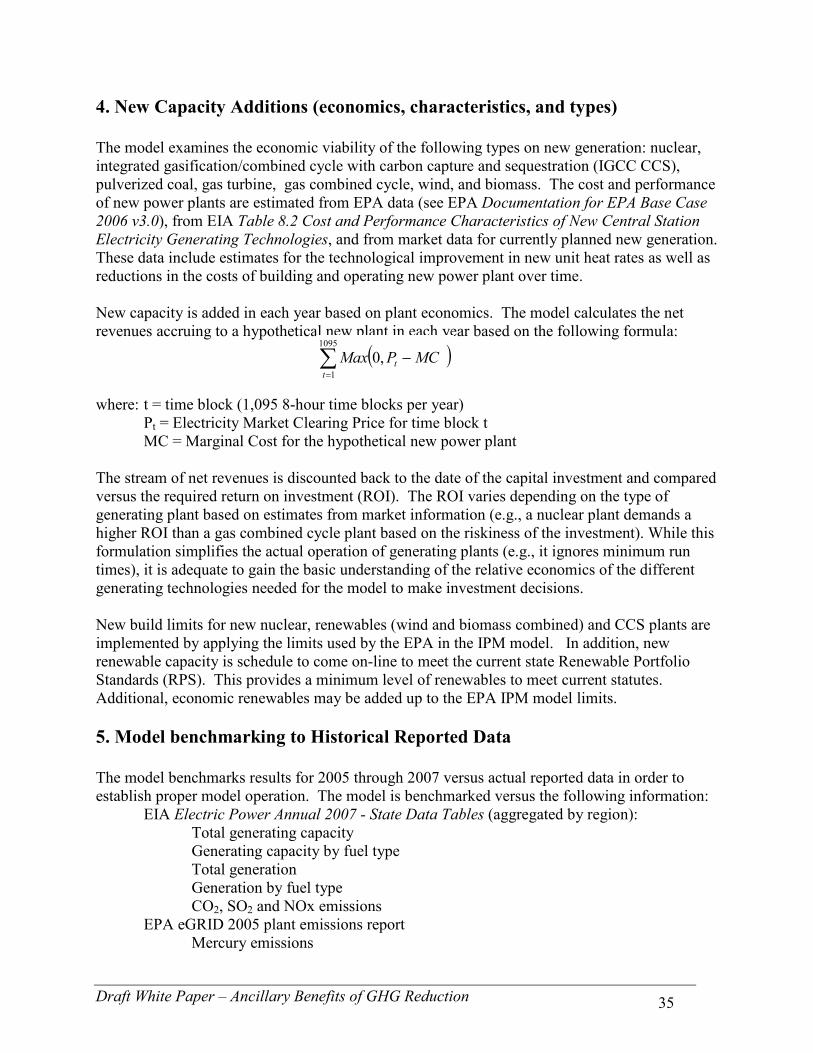
4. New Capacity Additions (economics, characteristics, and types) The model examines the economic viability of the following types on new generation: nuclear, integrated gasification/combined cycle with carbon capture and sequestration (IGCC CCS), pulverized coal, gas turbine, gas combined cycle, wind, and biomass. The cost and performance of new power plants are estimated from EPA data (see EPA Documentation for EPA Base Case 2006 v3.0), from EIA Table 8.2 Cost and Performance Characteristics of New Central Station Electricity Generating Technologies, and from market data for currently planned new generation. These data include estimates for the technological improvement in new unit heat rates as well as reductions in the costs of building and operating new power plant over time. New capacity is added in each year based on plant economics. The model calculates the net revenues accruing to a hypothetical new plant in each year based on the following formula: where: t = time block (1,095 8-hour time blocks per year) Pt = Electricity Market Clearing Price for time block t MC = Marginal Cost for the hypothetical new power plant The stream of net revenues is discounted back to the date of the capital investment and compared versus the required return on investment (ROI). The ROI varies depending on the type of generating plant based on estimates from market information (e.g., a nuclear plant demands a higher ROI than a gas combined cycle plant based on the riskiness of the investment). While this formulation simplifies the actual operation of generating plants (e.g., it ignores minimum run times), it is adequate to gain the basic understanding of the relative economics of the different generating technologies needed for the model to make investment decisions. New build limits for new nuclear, renewables (wind and biomass combined) and CCS plants are implemented by applying the limits used by the EPA in the IPM model. In addition, new renewable capacity is schedule to come on-line to meet the current state Renewable Portfolio Standards (RPS). This provides a minimum level of renewables to meet current statutes. Additional, economic renewables may be added up to the EPA IPM model limits. 5. Model benchmarking to Historical Reported Data The model benchmarks results for 2005 through 2007 versus actual reported data in order to establish proper model operation. The model is benchmarked versus the following information: EIA Electric Power Annual 2007 - State Data Tables (aggregated by region): Total generating capacity Generating capacity by fuel type Total generation Generation by fuel type CO2, SO2 and NOx emissions EPA eGRID 2005 plant emissions report Mercury emissions
( )∑=
−1095
1
,0t
t MCPMax
Draft White Paper – Ancillary Benefits of GHG Reduction 36
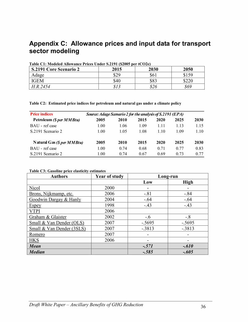
Appendix C: Allowance prices and input data for transport sector modeling Table C1: Modeled Allowance Prices Under S.2191 ($2005 per tCO2e) S.2191 Core Scenario 2 2015 2030 2050 Adage $29 $61 $159 IGEM $40 $83 $220 H.R.2454 $13 $26 $69
Table C2: Estimated price indices for petroleum and natural gas under a climate policy Price indices Source: Adage Scenario 2 for the analysis of S.2191 (EPA)Petroleum ($ per MMBtu) 2005 2010 2015 2020 2025 2030
BAU - ref case 1.00 1.06 1.09 1.11 1.13 1.15S.2191 Scenario 2 1.00 1.05 1.08 1.10 1.09 1.10
Natural Gas ($ per MMBtu) 2005 2010 2015 2020 2025 2030BAU - ref case 1.00 0.74 0.68 0.71 0.77 0.83S.2191 Scenario 2 1.00 0.74 0.67 0.69 0.73 0.77 Table C3: Gasoline price elasticity estimates
Authors Year of study Long-run Low High
Nicol 2000 - - Brons, Nijkmamp, etc. 2006 -.81 -.84 Goodwin Dargay & Hanly 2004 -.64 -.64 Espey 1998 -.43 -.43 VTPI 2006 Graham & Glaister 2002 -.6 -.8 Small & Van Dender (OLS) 2007 -.5695 -.5695 Small & Van Dender (3SLS) 2007 -.3813 -.3813 Romero 2007 - - HKS 2006 - - Mean -.571 -.610 Median -.585 -.605
Draft White Paper – Ancillary Benefits of GHG Reduction 37
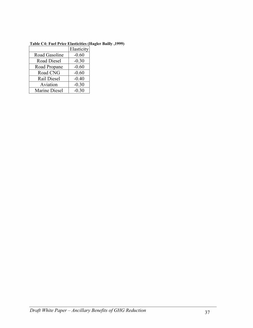
Table C4: Fuel Price Elasticities (Hagler Bailly ,1999)
Elasticity Road Gasoline -0.60 Road Diesel -0.30
Road Propane -0.60 Road CNG -0.60 Rail Diesel -0.40 Aviation -0.30
Marine Diesel -0.30
Draft White Paper – Ancillary Benefits of GHG Reduction 38
Appendix D: S.2191 as a “representative” climate policy Figure D.1
Source: http://pdf.wri.org/usclimatetargets_2008-12-08.pdf
Draft White Paper – Ancillary Benefits of GHG Reduction 39
Figure D.2: Comparison of Cumulative Emissions Ranges under Legislative Climate Change Targets in the 110th Congress (WRI)
Source: http://pdf.wri.org/usclimatetargets_2008-12-08.pdf