Estimating Willingness to Pay for E85 in the United States*

Kenneth Liao, Sébastien Pouliot, and Bruce Babcock

Working Paper 16-WP 562 Updated November 2016

Center for Agricultural and Rural Development Iowa State University

Ames, Iowa 50011-1070 www.card.iastate.edu

Kenneth Liao is a PhD candidate, Department of Economics, Iowa State University, Ames, IA 50011, E-mail: kliao@iastate.edu. Sébastien Pouliot is Associate Professor, Department of Economics, Iowa State University, Ames, IA 50011. E-mail: pouliot@iastate.edu. Bruce A. Babcock is Professor of Economics and Cargill Chair of Energy Economics and is the director of the Biobased Industry Center at Iowa State University, Ames, IA. E-mail: babcock@iastate.edu. This publication is available online on the CARD website: www.card.iastate.edu. Permission is granted to reproduce this information with appropriate attribution to the author and the Center for Agricultural and Rural Development, Iowa State University, Ames, Iowa 50011-1070. For questions or comments about the contents of this paper, please contact Kenneth Liao, kliao@iastate.edu.

Iowa State University does not discriminate on the basis of race, color, age, ethnicity, religion, national origin, pregnancy, sexual orientation, gender identity, genetic information, sex, marital status, disability, or status as a U.S. veteran. Inquiries can be directed to the Interim Assistant Director of Equal Opportunity and Compliance, 3280 Beardshear Hall, (515) 294-7612.

Estimating Willingness to Pay for E85 in the United States*

Kenneth Liao†

Sébastien Pouliot‡

and

Bruce A. Babcock§

November 11, 2016

Abstract: Meeting US ethanol blending mandates proposed by the Environmental Protection Agency will require a substantial number of motorists with flex-fuel vehicles to switch from low ethanol-gasoline blends to high ethanol-gasoline blends. The lower the willingness to pay for high-ethanol blends, the greater the cost of complying with the proposed mandates. Existing estimates of the willingness to pay for high-ethanol blends use data from Brazil (where consumers have knowledge of and experience with high-ethanol blends), data generated when retail prices greatly favored low-ethanol blends, or stated data collected from mail and online surveys. To obtain more accurate estimates of US willingness to pay, we conducted an intercept survey in five US states of motorists with flex-fuel vehicles as they were refueling. We address a sample-selection problem caused by the lack of stations that sell high-ethanol blends; consumers who have a high willingness to pay are more likely to seek out the stations and hence to show up in our sample. We attempt to overcome the problem caused by prices favoring low-ethanol blends by augmenting revealed preference data with stated preference data generated by hypothetical prices that tended to favor high-ethanol blends. Our estimates of mean willingness to pay shows that the price at which the average US consumer will switch fuels is substantially below the price that equates the cost per mile of driving. The large discount that the average US consumer requires to switch suggests that the cost of proposed ethanol mandates will be higher than previously estimated. Keywords: Biofuel, E85, Ethanol, Gasoline, Renewable Fuel Standard, Intercept Survey. JEL codes: Q18, Q41, Q42. Acknowledgements: We acknowledge support from the Biobased Industry Center at Iowa State University and the National Science Foundation under Grant Number EPS-1101284.

* Formerly titled “Willingness to Pay for Ethanol in Motor fuel: Evidence from Revealed and Stated Preference for E85.” † Visiting Assistant Professor, Department of Economics, Oberlin College. Email: kliao@oberlin.edu. ‡ Associate Professor, Department of Economics, Iowa State University. Email: pouliot@iastate.edu. § Cargill Endowed Chair of Energy Economics and Professor, Department of Economics, Iowa State University. Email: babcock@iastate.edu.

1

I. Introduction

The Renewable Fuel Standard (RFS) in the United States uses biofuel blending mandates to achieve its

policy objectives of reductions in greenhouse gas emissions, reductions in imports of fossil fuels, and

enhanced rural incomes. The blending mandates are set annually by the Environmental Protection

Agency (EPA) and must be met by gasoline producers (owners of oil refineries) and gasoline importers.

Mandate compliance is achieved by accumulating sufficient tradable permits, called Renewable

Identification Numbers (RINs). Gasoline producers can generate RINs by buying and blending biofuel, or

they can enter the market and buy RINs which are generated by blenders who are not obligated under

the RFS because they do not produce gasoline. Because each gallon of gasoline produced creates a RIN

obligation, the RIN price multiplied by the percentage blending requirement is the marginal tax burden

on gasoline producers. When mandates are binding, the RIN price is positive and covers the gap

between the marginal cost of producing biofuel and the marginal willingness to pay for biofuels by

blenders (Pouliot and Babcock 2016).1

Different mandates exist for different biofuels. EPA sets an overall renewable fuel mandate.

Within the overall mandate a separate mandate exists for advanced biofuels, which are defined by

whether they meet a greenhouse gas reduction target. The advanced mandate contains a separate

mandate for biomass-based diesel. The difference between the overall renewable fuel mandate and the

advanced biofuel mandate is often referred to as the conventional biofuel mandate or the corn ethanol

mandate because it can be met with corn ethanol. In 2015, the corn ethanol mandate could be met with

approximately 14 billion gallons of ethanol, whereas the advanced mandate could be met with

approximately two billion gallons of biomass-based diesel. Hence the corn ethanol mandate by far

receives the most attention by policy makers and industry.

Until 2016, the corn ethanol mandate was met by converting practically all US gasoline to E10,

which is a blend of 10 percent ethanol and 90 percent petroleum-based gasoline. In 2015, for example,

US gasoline consumption was 140.42 billion gallons (US EIA 2016) which means that the 14-billion-gallon

mandate could be met with the 14 billion gallons of ethanol consumed in E10. With practically all US

gasoline containing 10 percent ethanol by default, understanding consumer preferences about ethanol

had little urgency because the cost of meeting EPA blending mandates did not depend on inducing

consumers to choose fuel with greater concentration of ethanol per volume. However, EPA has

proposed future mandates that cannot be so easily met, and new controversies have arisen regarding

1 The EPA allows limited banking and borrowing of RINs. See Rubin (1996) for how intertemporal trading affects current RIN prices.

2

the feasibility of expanding biofuels volumes (Knittel et al. 2015; Pouliot and Babcock 2016). For 2017,

EPA has proposed a 14.8-billion-gallon corn ethanol mandate. With gasoline consumption forecasted to

be 143 billion gallons (US EIA 2016), ethanol consumption through E10 will fall at least 500 million

gallons short of the mandate.

The two approved alternative blends that could be used to increase ethanol consumption

beyond E10 levels are E15 and E85, which on average contain, respectively, 15 percent and 74 percent

ethanol. EPA is relying on increased E85 consumption to meet its ethanol blending mandate because so

few stations are equipped to sell E15. The cost and feasibility of meeting RFS blending targets depends

on consumer willingness to switch from E10 to E85. The decision to switch is complicated because fuel

efficiency with E85 is 22 percent lower than that of E10 because ethanol has one third less energy than

gasoline. The lower fuel efficiency also implies more frequent visits to the fuel station.

Salvo and Huse (2013) conduct an intercept survey of Brazilian motorists and estimate the

distribution of willingness to pay for E100 relative to E25, which are the fuel choices in Brazil. They find

that the median Brazilian motorist switches to E100 when its cost per mile falls below the cost per mile

of E25, which is consistent with a motorist who wants to minimize fuel costs. Pouliot and Babcock (2014)

use Brazilian preference data to estimate the demand for E85 in the United States to better understand

the feasibility of meeting increased ethanol mandates. Their study accounts for the fact that fewer than

10 percent of US vehicles are flex-fuel vehicles (FFVs) that can use E85 and the quite limited availability

of E85 across the country.2 FFVs are typically alternate versions of conventional models, and the

operation of an FFV is identical to the conventional version except for the lower fuel economy with E85.

Their finding that potential consumption of E85 in the United States can easily exceed one billion gallons

is dependent on the assumption that US motorists with FFVs have the same preferences for E85 as

Brazilian motorists.

There are many reasons why US motorists with FFVs may not have the same preferences as

Brazilian motorists. Almost all vehicles sold in Brazil since 2003 are flex vehicles, and almost all Brazilian

fuel stations sell both E100 and E25. Brazilians typically know when the cost per mile driving on E100 is

2 Until 2014, automobile manufacturers received a substantial credit from the US Corporate Average Fuel Economy (CAFE) standards for producing FFVs (Anderson and Sallee 2011). The credit started declining in 2015 and will cease in 2020. Under the rule, up to an annual limit, FFVs were treated as though they were operated partially on E85, but the fuel economy was calculated as the total miles the vehicle could travel per gallon of gasoline input (the ethanol fuel input was excluded in the fuel economy calculation). The result is that the majority of FFVs in the United States today are large sedans, SUVs, pickup trucks, and minivans, and they are mostly manufactured by American automobile companies.

3

lower than on E25. Thus the average Brazilian motorist has much more experience and information

about ethanol than does the average US flex motorist.

To better understand US preferences for E85 and whether they are consistent with Brazilian

preferences, we followed the example of Salvo and Huse (2013) and conducted an intercept survey of

US motorists in multiple states (Arkansas, California, Colorado, Iowa, and Oklahoma) as they refueled.

Our survey was designed to overcome circumstances not faced by Salvo and Huse (2013). In contrast to

Brazil, very few US stations sell E85. Thus many US flex motorists must incur additional costs to drive out

of their way to fill up with E85. This implies that our observed sample of flex motorists have, on average,

a higher willingness to pay for E85 than the population of flex motorists. We included questions in our

survey that allow us to correct for this selection bias.

Salvo and Huse (2013) were able to observe preferences for E100 when its cost per mile was

greater than E25 and when it was lower than E25. Thus they were able to estimate the distribution of

preferences more accurately than if their data had less variation in relative fuel costs. Estimations of US

preferences for E85 are hampered because it has been rare that the cost per mile of driving on E85 is

less than the cost per mile with E10. Anderson (2012) tried to overcome this difficulty by specifying a

parsimonious functional form for the distribution of preferences for E85 in Minnesota, but his data all

fell within one tail of his distribution.3 We overcome this lack of variation in relative prices by combining

revealed preference data with stated preference data. As part of our survey, fuel choices were

observed, and then we presented motorists with a hypothetical set of prices in an attempt to induce

them to switch fuels. By combining the stated preference data with the revealed preference data we can

much more precisely estimate the distribution of preferences for E85. However, because the

hypothetical prices were not randomized, but rather selected to induce switching, we must carefully

correct for the endogeneity problem created by our data collection method.

We find that US consumers have, on average, a much lower willingness to pay for high-ethanol

blends than the average Brazilian motorist. California motorists have a higher willingness to pay for E85

than motorists in the other four states surveyed. Corn Belt motorists located in Iowa do not have a

higher willingness to pay than motorists in Oklahoma, Arkansas, and Colorado. The policy implication of

our results is that the RIN price that is needed to induce enough consumption of ethanol to meet

proposed blending mandates is much higher than estimated by Pouliot and Babcock (2014) but that

3 Recent studies have used nationwide mail and online surveys to obtain stated-preference data on WTP for E85 (e.g., Jensen et al. 2010; Petrolia et al. 2010; Aguilar et al. 2015). However, these studies do not provide estimates of the distribution of WTP for E85 conditional on the relative prices of E10 and E85, and therefore their use is limited in policy analysis.

4

EPA’s proposed blending targets are feasible. We also examine whether motorists consider the relative

energy contents of E85 and E10 when making their fuel decisions and the impact of other factors that

explain variations in motorists’ willingness to pay.

II. Intercept Survey Design

We designed an intercept survey of motorists who drive FFVs at fuel stations that sell E85 to obtain data

on a broad range of factors that might affect willingness to pay for E85 as a substitute for E10. The

survey shares similarities with the survey of motorists at fuel stations in Brazil conducted by Salvo and

Huse (2013). After first observing motorists’ fuel choices from afar, we conducted an interview while

they refueled. We completed each interview in about two minutes which meant that, in almost every

case, we did not detain the motorists longer than the time it took to refuel. Appendix A contains the

complete questionnaire.

Intercept Survey Method

For each station we visited, we recorded station-level data including the station name and brand, the

station address, the prices of the E10 fuels (usually regular, midgrade, and premium), and the price of

E85. We conducted almost all of the interviews personally, and we made an effort to interview all of the

flex motorists who pulled alongside any of the station’s pumps. When a second flex motorist pulled up

to a pump during an interview, we did not interview the second flex motorist. Instead, when we

completed the first interview, we reset and then waited to interview the next flex motorist. This

sequencing rule avoided a selection bias. In practice, because the FFV-share of the vehicle fleet is small

and the survey was over quickly, we managed to capture virtually all of the flex motorists who visited

the E85 stations.

We visually identified FFVs in two ways. First, many newer FFVs have a badge on the back (or in

rare cases on the side) of the vehicle that indicates they are FFVs. Second, most FFVs have a yellow gas

cap, a yellow ring, or a yellow sticker inside the gas door indicating that it is capable of using E85. In

practice, identifying FFVs required the interviewer to walk around the pumps and closely inspect

vehicles as they were refueling. A third way to tell whether a vehicle was an FFV was if the motorist

chose E85. However, a few motorists made a fueling mistake by choosing E85 for a conventional vehicle

not equipped to use it or had a vehicle with aftermarket modifications to use E85.4

4 Over the course of conducting the survey, we learned that a small share of motorists have aftermarket modifications to conventional vehicles (not originally manufactured as FFVs) to use E85 because the higher octane

5

Before talking to a motorist, the interviewer passively observed each motorist’s fuel choice and

vehicle characteristics, including vehicle make, model, vehicle type (car, truck, SUV, or van), the state on

the license plate, whether the vehicle had an FFV badge, whether the vehicle had a yellow gas cap, and

the gender of the motorist. The interviewer also recorded the transaction volume and expenditure after

the motorist finished refueling.

Survey Questions

Once a motorist began refueling, the interviewer approached and asked whether the motorist was

willing to participate in a short survey. The interviewer then followed with a series of questions about

the motorist’s characteristics and motorist’s awareness of E85 and opinions on topics that might explain

the motorist’s fuel choice.5 Appendix B contains details about these questions.

We wanted to know if the motorists we surveyed were random draws from the general

population of flex motorists or if they were in our sample because they sought out E85. We know that

flex motorists who chose E10 did not come specifically to the station for E85, so we presume that they

would still have chosen to refuel at the particular station even if every station offered E85. We treat

these flex motorists as random draws from the local population of flex motorists. But for motorists who

chose E85 we asked, “Did you choose to fuel at this station because it offers E85?” If they responded

positively, we followed by asking, “How far out of your way did you have to drive?” We use responses to

these questions identify which motorists who chose E85 self-selected into the sample.

We asked a question to obtain stated preference (SP) data to complement the revealed

preference (RP) data by proposing a single hypothetical price scenario to each motorist. For motorists

who refueled with E10, the scenario was that we either increased the price of E10 or decreased the

price of E85. For motorists who refueled with E85, the scenario was that we either increased the price of

E85 or decreased the price of E10. The amount of the hypothetical price change was plus or minus

$0.25, $0.50, or $0.75 per gallon.

content can improve the vehicles’ (racing) performance. In most cases, the vehicles are modified so that they can use either E85 or E10, but in rare cases the vehicles are configured so that they can only use E85, and switching back to E10 requires modifying the vehicle. 5 In one question, we asked about ownership of the vehicle. We are particularly interested in identifying government vehicles because government employees driving an FFV are required to refuel with E85. Related to that, Corts (2010) shows that government fleet adoption of FFVs led to an increase in the number of retail E85 stations, but cannot say whether the increase in E85 stations led to an increase in motorists purchasing FFVs. Specifically, Corts (2010) notes that most FFVs in the dataset were purchased prior to the widespread availability of E85 and that flex motorists may not even know of their vehicles’ capabilities.

6

III. Sample Selection and Models of Fuel Choice

In this section, we discuss the sample-selection problem in our survey data and how we obtain a random

sample. We then describe motorists’ fuel choices in random utility models. We develop two alternative

models in which motorists make their fuel decisions based on either 1) the difference in the price of E85

and E10, which we call the E85 premium, or 2) the ratio of the price of E85 to E10, which we call the E85

ratio. We estimate models that are consistent with these two decision models and compare model fits

to determine how motorists make their fuel decisions.

Sample Selection

Recall that we only surveyed flex motorists at stations that sold E85. The sample-selection problem

arises from motorists self-selecting into the survey because of their high willingness to pay for E85. In

the United States in 2014 and 2015 (when we conducted our survey) there were about 2,700 fuel

stations that offered E85 while E10 was available in all of the nearly 110,000 fuel stations. Motorists

could access E10 at any station along their normal driving routes. However, most motorists could not

access E85 at what would otherwise be their most preferred or most convenient station, so many

motorists had to deviate from normal driving routes or break from their normal refueling habits to

access E85. Thus, many flex motorists who we observed refueling with E85 incurred costs associated

with forgoing E10-only stations.

The motorists in our survey who chose E10 had the opportunity to refuel with E10 at any other

station, and their patronage of the surveyed station was not motivated by its offering of E85.6 For these

motorists, the opportunity cost of accessing E10 at the surveyed fuel station was zero. Likewise, for

several motorists we surveyed who chose E85, the surveyed station was the same station where they

would have fueled even if E85 was offered at every station. These motorists did not self-select into our

sample. The motorists who self-selected into our survey were those who would not have refueled at the

surveyed station except for the fact that it offered E85. For these motorists, there was an opportunity

cost of refueling with E85, so they purchased E85 only if the value they assigned to E85 over E10 (given

prices) exceeded the cost of accessing E85. This means that the intercept survey over-sampled motorists

6 It is conceivable that some of the flex motorists who chose E10 may have chosen to refuel at the E85 station specifically because it offered E85 because they wanted the E85 option and would have chosen E85 if the relative price on that particular day had been more favorable. But in talking to the E10 motorists about hypothetical prices and choices, refueling habits, and knowledge of E85, we rarely encountered motorists who could claim this behavior. Instead, some E10 motorists did not know they had FFVs, that the station offered E85, or really what E85 was. The flex motorists who were deciding between E85 and E10 seemed to be generally aware of the prevailing fuel prices and seemed to make their fuel choices before arriving at the station and viewing the exact prices.

7

who chose E85, especially those with high willingness to pay for E85. A further implication is that the

distribution of preferences among E85 motorists who self-selected into the sample has mean willingness

to pay that is higher than the mean willingness to pay for the distribution of preferences among E85

motorists who did not self-select into the sample.

Recall that we asked motorists who chose E85 two questions to inform self-selection. The first

question was, “Did you choose to fuel at this station because it offers E85?” To the motorists who

answered “yes,” we followed by asking, “How far out of your way did you have to drive?” We determine

which motorists constitute a random sample based on the answers to these questions.

Using motorists’ responses to the first question to select a random sample may be too

restrictive because of how motorists interpreted the question. It is possible that some motorists who

answered “yes” to the question about whether their patronage was motivated by the offering of E85

would have chosen the same station even if E85 were offered at every station. Indeed, many motorists

answered the follow-up question about how far out of their way they drove to access E85 with, “Not at

all,” “I didn’t,” or “Zero.” The true random sample therefore likely consists of all of the motorists who

chose E10, all of the motorists who chose E85 and answered “no” to the first question, and some of the

motorists who chose E85, answered “yes” to the first question, and answered (some form of) “zero” to

the second question.

We cannot determine which of the motorists who answered “zero” to the second question

should be part of what constitutes a random sample. Our approach will be to compare models where

the random sample includes the E10 motorists and only the E85 motorists who answered “no” to the

first question to models where the sample also includes E85 motorists who answered “yes” to the first

question and “zero” to the second question. Using these two competing estimation samples, we will

estimate bounds on the population parameters and mean willingness to pay.

One could consider modeling the selection problem so that the empirical model uses the full

sample of data. However, this would require either knowing how much it costs consumers to drive to an

out-of-the-way fuel station or making identification of such transportation costs possible. One important

difficulty in the identification of consumer transportation cost is that in the sample the distance driven

to access E85 is positively correlated with the motorists’ choice of E85. In the population for FFV

motorists, this correlation is negative. Instead of imposing strong assumption on the model to make

identification of the transportation cost possible, we elect to work with smaller data samples that are

nearly representative of the population of flex motorists.

8

If driving costs were zero, the distribution of preferences among motorists who self-selected

into the sample for E85 would be the same as the distribution of preferences among the motorists who

were random draws from the population and chose E85. In such a world, we could include the extra

observations where motorists self-selected into our sample and use a model that corrects for the

choice-based sampling. The problem of the stratified sampling that would occur with those data has

been described and estimators have been proposed in prior literature (e.g. Manski and Lerman 1977;

Manski and McFadden 1981; Imbens 1992; Imbens and Lancaster 1996). But driving costs do not equal

zero and can be quite significant (e.g. Houde 2012; Wolff 2014). And because of driving costs, the

distribution of preferences among the E85 motorists who self-selected into the sample is not the same

as that of the E85 motorists who were random draws from the population. This violates a fundamental

assumption in models of choice-based sampling.

Models of Motorists’ Fuel Choice

The random utility models below show how motorists make their choices when they select a fuel based

on either the E85 premium or the E85 ratio. The model focuses on fuel choices and assumes that the

demand for fuel is perfectly inelastic in the short run. That is, motorists choose either E85 or E10 based

on the E85 premium or the E85 ratio but the amount of fuel they purchase is price-independent. We

consider only motorists who do not incur a cost to access the E85 station, for whom the E85 station

would be the most preferred station even if every station offered E85. Thus we do not consider the

motorists’ decisions of which fuel station to visit. Throughout, we use subscript 𝑒𝑒 to denote E85 and a

subscript 𝑔𝑔 to denote E10.

In the E85 premium model, the indirect utility that motorist 𝑖𝑖 derives from consumption of fuel

𝑗𝑗 ∈ {𝑒𝑒,𝑔𝑔} takes a linear form and is given by

𝑉𝑉𝑖𝑖𝑖𝑖�𝑝𝑝𝑖𝑖𝑖𝑖 , 𝐱𝐱𝐢𝐢, 𝜀𝜀𝑖𝑖𝑖𝑖� = 𝛼𝛼𝑖𝑖𝑝𝑝𝑖𝑖𝑖𝑖 + 𝐱𝐱𝐢𝐢′𝛃𝛃𝐣𝐣 + 𝜀𝜀𝑖𝑖𝑖𝑖 (1)

where 𝑝𝑝𝑖𝑖𝑖𝑖 is the nominal price of fuel 𝑗𝑗 for motorist 𝑖𝑖, 𝐱𝐱𝐢𝐢 is a vector of characteristics about the motorist

and the fueling station, and 𝜀𝜀𝑖𝑖𝑖𝑖 is an unobservable stochastic shifter specific to the motorist and fuel

choice. We assume that 𝜀𝜀𝑖𝑖𝑖𝑖 is a type 1 generalized extreme value random variable so that the difference

between 𝜀𝜀𝑖𝑖𝑖𝑖 and 𝜀𝜀𝑖𝑖𝑖𝑖 follows a logistic distribution. We let 𝛼𝛼𝑖𝑖 = 𝛼𝛼𝑖𝑖 ≡ 𝛼𝛼 so that that motorists’ fuel

choices do not depend on individual fuel prices but rather on the difference in the fuel prices. We let

𝛃𝛃 ≡ 𝛃𝛃𝐞𝐞 − 𝛃𝛃𝐠𝐠, and we define 𝑑𝑑𝑖𝑖 ≡ 𝑝𝑝𝑖𝑖𝑖𝑖 − 𝑝𝑝𝑖𝑖𝑖𝑖 to be the E85 premium observed by motorist 𝑖𝑖. A motorist

chooses E85 if 𝑉𝑉𝑖𝑖𝑖𝑖(∙) ≥ 𝑉𝑉𝑖𝑖𝑖𝑖(∙) which amounts to

𝛼𝛼𝑑𝑑𝑖𝑖 + 𝐱𝐱𝐢𝐢′𝛃𝛃 ≥ 𝜀𝜀𝑖𝑖,

9

where 𝜀𝜀𝑖𝑖 ≡ 𝜀𝜀𝑖𝑖𝑖𝑖 − 𝜀𝜀𝑖𝑖𝑖𝑖 is symmetric with a mean of zero and follows a logistic distribution.

In the price ratio model, the indirect utility flex motorist 𝑖𝑖 derives from fuel 𝑗𝑗 is

𝑉𝑉�𝑖𝑖𝑖𝑖�𝑝𝑝𝑖𝑖𝑖𝑖 , 𝐱𝐱𝐢𝐢, 𝑒𝑒𝑖𝑖𝑖𝑖� = 𝑝𝑝𝑖𝑖𝑖𝑖𝑎𝑎𝑗𝑗 ∙ 𝐱𝐱𝐢𝐢𝐛𝐛𝐣𝐣 ∙ exp�𝑒𝑒𝑖𝑖𝑖𝑖�, (2)

where again 𝑒𝑒𝑖𝑖𝑖𝑖 is a type 1 extreme value random variable. Taking logs on both sides, we can write that

a motorist chooses E85 if log𝑉𝑉�𝑖𝑖𝑖𝑖(∙) ≥ log𝑉𝑉�𝑖𝑖𝑖𝑖(∙) or

𝑎𝑎 log(𝑟𝑟𝑖𝑖) + log(𝐱𝐱𝐢𝐢′)𝐛𝐛 ≥ 𝑒𝑒𝑖𝑖,

where 𝑟𝑟𝑖𝑖 ≡ 𝑝𝑝𝑖𝑖𝑖𝑖/𝑝𝑝𝑖𝑖𝑖𝑖 and 𝑒𝑒𝑖𝑖 ≡ 𝑒𝑒𝑖𝑖𝑖𝑖 − 𝑒𝑒𝑖𝑖𝑖𝑖. Thus, in the ratio model, preferences also follow a logistic

distribution but the variables enter the model in logs.

IV. Data Collection and Summary Statistics

We obtained the cooperation of two E85 retailers to conduct our survey. We collected a total of 972

observations of flex motorists from 17 E85 stations in six urban areas between October 2014 and April

2015.7 In chronological order, the urban areas we visited were: Ames/Des Moines, Iowa; Colorado

Springs, Colorado; Tulsa, Oklahoma; Little Rock, Arkansas; Sacramento, California; and Los Angeles,

California. We personally collected most of the observations. A small team of undergraduate students

helped collect some of the observations in the Ames/Des Moines area. In each urban area, we visited

between two and four stations and collected around 100 or more observations. All of the E85 stations

we visited in Arkansas, Colorado, Iowa, and Oklahoma were operated by a retailer we will call ‘Retailer

Y’, and all of the E85 stations we visited in California were operated by a retailer we will call ‘Retailer Z’.

Observed Data and Survey Responses

From the initial 972 observations of motorists refueling their FFVs, we remove 79 observations where

motorists chose not to or were unable to complete or participate in the survey. This represents a total

non-response rate of 8 percent. We also remove 12 observations for which we do not have SP data

either because we asked the question incorrectly or the motorist was unable to answer. That leaves us

with an initial sample of 881 complete observations before we address the sample-selection problem.

Table 1 summarizes the fuel choice data broken down by station, urban area, and retailer. In the entire

sample of 881 flex motorists, the average E85 price was $2.19 per gallon, and the average E10 price was

$2.58 per gallon. Therefore, the average E85 premium (defined as the E85 price per gallon minus the

7 We collected a total of 994 observations, but 22 were from conventional vehicles with aftermarket modifications to use E85. We observed these vehicles refueling with E85, but we exclude these observations because we can only identify the vehicles as flex when the motorists choose E85.

10

E10 price per gallon) was -$0.39. The average E85 ratio (defined as the E85 price divided by the E10

price) was 0.85. Overall, 431 (49 percent) of flex motorists chose E85 while 450 (51 percent) chose E10.8

On average fuel prices were more favorable toward E85 at Retailer Z’s stations where the

average E85 premium was -$0.54, and the E85 ratio was 0.83. We observed 231 flex motorists refueling

at Retailer Z’s locations, and 89 percent chose E85. Retailer Z’s E85 prices were not drastically more

favorable than Retailer Y’s E85 prices, but each of Retailer Z’s pumps served a larger share of the local

E85-choosing community of flex motorists because E85 stations were less common in California. Also,

Retailer Z ran promotions providing special fuel cards and other incentives to local flex motorists,

marketing E85 as a clean-burning, high-performance fuel. We do not have evidence that any particular

promotion was taking place while we conducted the survey.

For Retailer Y, E85 prices were lowest in Iowa, where the average E85 premium was -$0.47, and

the average E85 ratio was 0.83, the same as the average price ratio observed at Retailer Z’s stations.

Absolute fuel prices were higher in California, so the California E85 premium was larger in magnitude.

The share of flex motorists who chose E85 among Iowa flex motorists was 42 percent, less than half of

what we observed at E85 stations in California. We suspect that one reason for the difference is that

stations that offer E85 are more common in Retailer Y’s areas. Thus local flex motorists with high

willingness to pay for E85 can choose between multiple E85 stations and will not all be observed in the

sample.

Recall that we do not consider all interviewed motorists as random draws from the population

of flex motorists. Instead, we have two rules that we use to identify and select motorists. The first rule is

more restrictive and only motorists who answered that they did not go out of their way to the fuel

station for E85 are part of the sample. Using that rule leaves us with a total 479 observations with 29

motorists selecting E85. The second rule is more inclusive and uses observations where motorists

answered zero to the question about how far out of their way they drove to fuel with E85. This second

rule gives us a sample of 670 observations with 220 motorists selecting E85.

Figure 1 shows the share of motorists who chose to refuel with E85 (RP choice) as a function of

the E85 premium for the more inclusive sample with 670 observations. The corresponding figure with

the sample of 479 observations is similar. We only show the figure for the E85 premium, but the figure

for the E85 ratio is practically identical. Figure 1 shows that the share of motorists who chose E85 at

Retailer Y declines with respect to the E85 premium as expected and ranges from a bit above zero to

8 Among the 450 flex motorists who chose E10, 414 (92 percent) chose regular grade 87 octane (85 octane in CO), 24 (5 percent) chose midgrade, and 12 (3 percent) chose premium.

11

almost 50 percent. At Retailer Z, the share of motorists who refuel with E85 increases with respect to

the E85 premium. The variation in the E85 premium is small however, which might explain why we

observe a positive slope. The share of motorists who refuel with E85 at Retailer Z is above 50 percent for

all observed E85 premium values.

Figure 2 shows in two panels the share of motorists who chose to fuel with E85 as a function of

the hypothetical E85 premium for the more inclusive sample with 670 observations. The hypothetical

price scenario that we presented to motorists was conditional on their fuel choice and accordingly we

present the shares conditional on motorists’ fuel choice (RP choice). One of our empirical model

accounts specifically for this. Observe that in both panels of Figure 2, variations in hypothetical prices

are much greater than the variation in prices in Figure 1. Panel a) of Figure 2 is for observations we

collected at Retailer Y and shows that the share of motorists who chose E85 declines with respect to the

hypothetical E85 premium regardless of whether motorists’ RP choice was E10 or E85. Panel b) is for

observations we collected at Retailer Z. The share of motorists who chose E85 declines with respect to

the hypothetical E85 premium for those who refueled with E85 but unexpectedly increased for those

who refueled with E10.

V. Empirical Models

In this section, we describe four empirical models that we use to obtain estimates of the distribution of

willingness to pay for E85. The models differ depending on whether we apply a correction for the rare

occurrence of E85 and whether we use the SP data.

In the description of the empirical models, we will use a generic notation for both the premium

and the ratio models where 𝛬𝛬(∙) is the cumulative logistic distribution, iz is the vector of dependent

variables that includes either the E85 premium or the log of the E85 ratio, and θ is the vector of

parameters to estimate. We write that iy equals one for a motorist who refuels with E85, and iy

equals zero for a motorist who refuels with E10.

Maximum Likelihood

The first model we consider is the standard maximum likelihood estimator (MLE). Under standard

assumptions, 𝐳𝐳𝐢𝐢 is exogenous so we can consistently estimate 𝛉𝛉 by maximizing the conditional log-

likelihood given by

12

( ) ( ) ( ) ( ){ }1 1

log ln 1 ln 1 lnN N

i i ii i

L f y y y= =

′ ′= = − −Λ + Λ ∑ ∑i i iz ,θ z θ z θ . (3)

This is the log-likelihood we will use to estimate models with the RP data only. It does not correct for the

bias from the rare-choice problem discussed next.

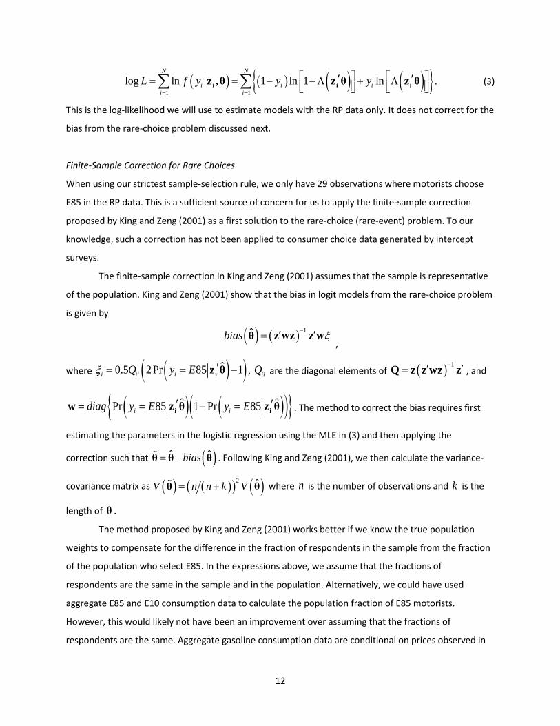
Finite-Sample Correction for Rare Choices

When using our strictest sample-selection rule, we only have 29 observations where motorists choose

E85 in the RP data. This is a sufficient source of concern for us to apply the finite-sample correction

proposed by King and Zeng (2001) as a first solution to the rare-choice (rare-event) problem. To our

knowledge, such a correction has not been applied to consumer choice data generated by intercept

surveys.

The finite-sample correction in King and Zeng (2001) assumes that the sample is representative

of the population. King and Zeng (2001) show that the bias in logit models from the rare-choice problem

is given by

( ) ( ) 1ˆbias ξ−′ ′=θ z wz z w ,

where ( )( )ˆ0.5 2Pr 85 1i ii iQ y Eξ ′= = −iz θ , iiQ are the diagonal elements of ( ) 1−′ ′=Q z z wz z , and

( ) ( )( ){ }ˆ ˆPr 85 1 Pr 85i idiag y E y E′ ′= = − =i iw z θ z θ . The method to correct the bias requires first

estimating the parameters in the logistic regression using the MLE in (3) and then applying the

correction such that ( )ˆ ˆbias= −θ θ θ . Following King and Zeng (2001), we then calculate the variance-

covariance matrix as ( ) ( )( ) ( )2 ˆV n n k V= +θ θ where n is the number of observations and k is the

length of θ .

The method proposed by King and Zeng (2001) works better if we know the true population

weights to compensate for the difference in the fraction of respondents in the sample from the fraction

of the population who select E85. In the expressions above, we assume that the fractions of

respondents are the same in the sample and in the population. Alternatively, we could have used

aggregate E85 and E10 consumption data to calculate the population fraction of E85 motorists.

However, this would likely not have been an improvement over assuming that the fractions of

respondents are the same. Aggregate gasoline consumption data are conditional on prices observed in

13

the past and as such are likely not to apply when we conducted the survey. Moreover, the level of

aggregation of E85 and E10 consumption data might be too high and thus fractions from those data may

not be appropriate for the areas where we conducted our survey.

King and Zeng (2001) recommend using their method even when there is no apparent rare-

choice problem. The arguments are that their method is simple to implement and that there is no

sample size large enough to evade the finite sample-size problem if an event is sufficiently rare. For

these reasons, not only will we use the finite-sample correction on the MLE but also on the coefficients

estimated with the SP-off-RP approach we describe below.

Two Methods for Augmenting RP Data with SP Data

Our second solution to the rare-choice problem is to augment our RP data with SP data. As we will show,

the MLE in (3) is not a correct approach for estimation of models that add SP data.

SP data have been used to complement RP data in previous studies to increase the number of

observations and expand the choice set to include alternative(s) that are sometimes not available on the

market. The traditional method for estimating models using combined RP and SP data in the

transportation and the environmental economic literature has been described by Ben-Akiva and

Morikawa (1990), Hensher and Bradley (1993), Adamowicz et al. (1994), and Hensher et al. (1999). The

intuition behind the traditional approach is that the unobserved factors are different for the two types

of data. To account for this, the RP and SP data are stacked together and the empirical model allows for

different intercept and scale parameters for the distributions of error terms for the SP and RP data. This

traditional approach is appropriate when the attributes of the hypothetical choices in the SP data

collection are independent of the RP choices so that respondents’ unobservable characteristics are not

correlated with the hypothetical options.

Train and Wilson (2008) and Train and Wilson (2009) consider SP data constructed from RP

choices. They refer to these data as “SP-off-RP” data. The important distinction from the traditional SP

data is that the hypothetical choice scenario depends on the consumer’s observed choice, which causes

an endogeneity problem. Recall that in our case, if we observed a motorist choosing E10, we offered

hypothetical prices that were more favorable to E85. If we observed a motorist choosing E85, we

offered hypothetical prices that were more favorable to E10. A motorist’s RP fuel choice depends on

both observed characteristics and unobservable factors. The same unobservable factors that affect the

motorist’s observed RP fuel choice (and therefore the hypothetical prices) carry over to the SP

14

experiment, so that the unobserved factors in the SP experiment are correlated with the hypothetical

prices, and we need to account for this when incorporating the SP data.

We define the utility that flex motorist 𝑖𝑖 derives from fuel 𝑗𝑗 in the SP experiment as

𝑊𝑊𝑖𝑖𝑖𝑖���𝐳𝐢𝐢𝐣𝐣, 𝜀𝜀𝑖𝑖𝑖𝑖 , 𝜂𝜂𝑖𝑖𝑖𝑖� = ��𝐳𝐢𝐢𝐣𝐣′𝛉𝛉𝐣𝐣 + 𝜀𝜀𝑖𝑖𝑖𝑖 + 𝜂𝜂𝑖𝑖𝑖𝑖,

where ijz is the vector of dependent variables that includes either the hypothetical E85 premium or the

hypothetical E85 ratio calculated from the hypothetical prices ��𝑝𝑖𝑖𝑖𝑖 and ��𝑝𝑖𝑖𝑖𝑖, and 𝜂𝜂𝑖𝑖𝑖𝑖 is a generalized

extreme random variable with scale (1/ 𝜁𝜁) that captures additional unobservable aspects of the SP

scenario not present in the RP scenario. Note that in the SP data, the relationships between both the

observable and unobservable factors that determine the utility in the RP data in 𝑉𝑉𝑖𝑖𝑖𝑖(∙) in equations (1)

and (2) are preserved. This means that the unobservable 𝜀𝜀𝑖𝑖𝑖𝑖 term for motorist 𝑖𝑖 that affects the RP

choice carries forward to the SP choice. The total unobservable error term in the SP model is 𝜀𝜀𝑖𝑖𝑖𝑖 + 𝜂𝜂𝑖𝑖𝑖𝑖,

where 𝜀𝜀𝑖𝑖𝑖𝑖 derives from the motorist’s RP choice. We use that choice to generate the hypothetical prices

��𝑝𝑖𝑖𝑖𝑖 and ��𝑝𝑖𝑖𝑖𝑖 in the SP experiment. Thus the hypothetical prices in the SP data are endogenous because

they are correlated with the total error term, 𝜀𝜀𝑖𝑖𝑖𝑖 + 𝜂𝜂𝑖𝑖𝑖𝑖.

A motorist chooses E85 in the hypothetical price scenario if 𝑊𝑊𝑖𝑖𝑖𝑖(∙) ≥ 𝑊𝑊𝑖𝑖𝑖𝑖(∙), which we can re-

write as

𝜁𝜁(��𝐳𝐢𝐢′𝛉𝛉 − 𝜀𝜀𝑖𝑖) ≥ 𝜂𝜂𝑖𝑖,

where 𝜂𝜂𝑖𝑖 ≡ 𝜁𝜁�𝜂𝜂𝑖𝑖𝑖𝑖 − 𝜂𝜂𝑖𝑖𝑖𝑖� is symmetric with a mean of zero and follows a logistic distribution. The 𝜁𝜁 term

normalizes the logistic distribution of 𝜂𝜂𝑖𝑖 to have a scale of one. The probability that a motorist chooses

E85 in the experiment is Pr(SP E85𝑖𝑖) = 𝛬𝛬(𝜁𝜁[��𝐳𝐢𝐢′𝛉𝛉 − 𝜀𝜀𝑖𝑖]), and the probability that a motorist chooses

E10 in the experiment is Pr(SP E10𝑖𝑖) = 1 − 𝛬𝛬(𝜁𝜁[��𝐳𝐢𝐢′𝛉𝛉 − 𝜀𝜀𝑖𝑖]). The joint probability of a motorist’s

specific RP and SP choice combination is the product of the probability of the RP choice and the

conditional probability of the SP choice (conditional on the RP choice). We write ( )1 2,i i iy y y= where

1iy is the RP choice and 2iy is the SP choice. The SP-off-RP likelihood function is

( ) ( )( )

( ) ( )( )

( ) ( )( )

( ) ( )( )

i i i i i i0,0 0,1

i i i i i i1,0 1,1

Pr RP E10 Pr SP E10 RP E10 Pr RP E10 Pr SP E85 RP E10

Pr RP E85 Pr SP E10 RP E85 Pr RP E85 Pr SP E85 RP E85 .i i

i i

y y

y y

L= =

= =

= ∏ ∏

∏ ∏

(4)

The 𝜀𝜀𝑖𝑖’s that enter the SP probability expressions are not observed but we know their conditional

distributions so we can integrate over the density to calculate the expected value of the logits given the

15

correlated errors. For example, the logit probability of a motorist choosing E85 in the SP experiment

conditional on that motorist choosing E85 in the RP data is

Pr(SP E85𝑖𝑖|RP E85𝑖𝑖) = 𝛬𝛬(𝜁𝜁[��𝐳𝐢𝐢′𝛉𝛉 − 𝜀𝜀𝑖𝑖|𝜀𝜀𝑖𝑖 ≤ 𝐳𝐳𝐢𝐢′𝛉𝛉]),

which we can write as

Pr(SP E85𝑖𝑖|RP E85𝑖𝑖) = ∫𝛬𝛬(𝜁𝜁[��𝐳𝐢𝐢′𝛉𝛉 − 𝜀𝜀𝑖𝑖]) 𝜆𝜆(𝜀𝜀𝑖𝑖|𝜀𝜀𝑖𝑖 ≤ 𝐳𝐳𝐢𝐢′𝛉𝛉)𝑑𝑑𝜀𝜀𝑖𝑖,

where 𝜆𝜆(∙) is the marginal density of the logistic distribution. We evaluate the integrals by simulation,

taking draws of 𝜀𝜀𝑖𝑖 from its conditional density following the method described by Train and Wilson

(2009). The probability 𝛬𝛬(∙) is calculated for each draw and the results are averaged. We estimate the

parameters by maximizing the log of the likelihood function in equation (4) using 1,000 conditional

logistic draws for each observation.

VI. Estimation Results

In this section, we present estimates of the empirical models described in the previous section. We

identify and present the models in the following manner: A) MLE with the RP data only; B) finite-sample

correction on the estimates in A); C) traditional augmentation of RP data with SP data; and D) SP-off-RP

method for data augmentation. We add a model: E) finite-sample correction on the estimates in D) to

investigate whether applying the finite-sample correction had much of an impact when using the SP-off-

RP approach.

Each model uses the following explanatory variables: vehicle ownership (personal, government,

company, other), vehicle type (car, truck, SUV, van), whether the vehicle had an FFV badge, number of

miles driven per year, gender, age, opinions about which fuel is better for the environment, the engine,

the economy, or national security, opinion on which fuel yields more miles per gallon, and the state

where the station was located (Arkansas, California, Colorado, Iowa, or Oklahoma). We do not include

the variables that describe the characteristics of the fuel stations because the state dummies summarize

most of that information.

We will not show results for all of the estimated coefficients, but the interested reader can refer

to Appendix C for complete results. Rather, we will focus on parameters that summarize the distribution

of preferences. We report the location and the scale parameters that summarize the logistic distribution

(for the E85 premium models) and the scale and shape parameters that summarize the log-logistic

distribution (for the E85 ratio models). The location parameter in the premium models and the scale

parameter in the ratio models summarize motorists’ perceptions of the value of E85 relative to E10.

16

These parameters are straightforward to interpret, and their values can be directly used in models for

policy analysis.

For the premium models, we calculate the mean of the logistic willingness to pay distribution as

( )1 ˆ ˆN iµ α′= −∑ ix β , where N is the number of observations, and the scale parameter as ˆ1s α= − .

Similarly, for the ratio models, we calculate the scale parameter as ( )( )1 ˆ ˆexp logN iaρ ′= −

∑ ix b

and the shape parameter as aσ = − . We expect the propensity to purchase E85 to decline with respect

to the price of E85 relative to E10 such that ˆ 0α < and ˆ 0a < . Thus, because we must have that 0s >

and 0σ > , we add a negative sign in front of α and a in our calculations of the distribution

parameters. Alternatively, we could have defined the price variables as the price of E10 minus the price

of E85 or the price of E10 divided by the price of E85. We calculate the standard errors of the

distribution parameters using the delta-method.9

We compare Retailer Y and Retailer Z using the estimated location parameters in the E85

premium models and the estimated scale parameters in the E85 ratio models. We find moderate

differences in the location parameters for the four states where we conducted interviews at Retailer Y.

However, these differences are small when compared to the difference in the value of the location

parameter for motorists in California buying fuel from Retailer Z. Thus, we will focus the discussion on

summarizing the willingness to pay distribution at all of Retailer Y’s locations collectively relative to

willingness to pay at Retailer Z’s locations in California.

For the premium models, given an average price of E10 of $2.38 per gallon at Retailer Y, a value

for the location parameter below negative $0.52 per gallon indicates that the average motorist prefers

E10 to E85 when prices are equal on a cost-per-mile basis. With an average E10 price of $3.12 per gallon

at Retailer Z, a mean willingness to pay below negative $0.70 per gallon indicates that the average

motorist prefers E10 to E85 when prices are at cost-per-mile parity. For the ratio models, a value for the

scale parameter below 0.78 indicates that the median motorist prefers E10 to E85 at cost-per-mile price

parity.

We begin with the estimates of the distribution parameters with the sample of 479 observations

in Table 2. Looking at the location parameters for the premium models, observe that across all models

9 We also calculated the standard errors in models A, B and C by bootstrap, and the bootstrap standard errors are smaller than the standard errors from using the delta-method. However, we do not report bootstrap standard errors because their calculation is too computationally intensive in models D and E (which we integrate by simulation) even when the number of draws is low.

17

the average motorist discounts E85 relative to E10 by about $1.80 per gallon at Retailer Y and by about

$1.00-1.20 per gallon at Retailer Z. These are large discounts because the average price of E10 was

about $2.38 per gallon at Retailer Y and $3.12 per gallon at Retailer Z. Comparing Models 1-A and 1-B,

the effect of the finite-sample correction is that it increases the estimated values of both the location

and scale parameters without improving the precision.

In Model 1-C, where we estimate the model using the traditional approach of stacking up the RP

and the SP data, we find values for the location and scale parameters not too different from those in

Model 1-A, but the standard errors are much smaller. The model for the SP-off-RP data we show above

demonstrates the endogeneity problem created from the collection of the SP data. This endogeneity

problem does not appear too large based on the comparison of the estimated distribution parameters

of Model 1-C to those of Model 1-A. However, looking at individual regression coefficients or the

marginal effects in Appendix C, the difference is more apparent.

Model 1-D yields values for the mean willingness to pay that are lower than those in Model 1-A,

and the estimated value for the scale parameter is larger than in Model 1-A. Furthermore, the standard

errors in Model 1-D are much smaller than those in Model 1-A. Comparing the estimated distribution

parameters of Model 1-E to those of Model 1-D, we find that the finite-sample correction has an effect

similar to the one we obtained between Model 1-A and Model 1-B.

Estimates of the log-logistic distribution parameters in Table 2 also show that motorists

significantly discount E85. Recall that prices are in cost-per-mile parity when the price ratio is 0.78.

Estimates of the scale parameter, which is the median of the log-logistic distribution, are far below the

parity price ratio. MLE in Model 2-A yields a median for the distribution of willingness to pay of 0.51 at

Retailer Y and 0.68 at Retailer Z. The distribution of willingness to pay is wide with an estimated value

for the shape parameter of 7.84. The finite-sample correction in Model 2-B slightly increases the value

of the scale parameters and reduces the value of the shape parameter. When stacking the RP and SP

data, the median willingness to pay declines to 0.44 at Retailer Y and to 0.55 at Retailer Z and a smaller

value for the shape parameter at 6.12. The standard errors in Model 2-C are much smaller than those in

Model 2-A. Compared to Model 2-A, the SP-off-RP estimates in Model 2-D of the scale parameter and

shape parameter are smaller and more precisely estimated. Applying a finite-sample correction to

Model 2-D, the estimate in Model 2-E for the scale parameter increases, but the estimate of the shape

parameter declines.

Table 3 shows estimates of the willingness to pay distribution parameters using the sample of

670 observations. The estimates in Table 3 for the location parameter for the E85 premium models and

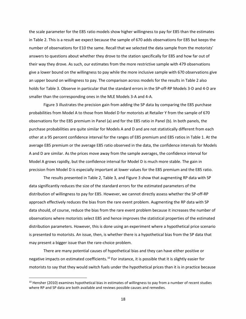
18

the scale parameter for the E85 ratio models show higher willingness to pay for E85 than the estimates

in Table 2. This is a result we expect because the sample of 670 adds observations for E85 but keeps the

number of observations for E10 the same. Recall that we selected the data sample from the motorists’

answers to questions about whether they drove to the station specifically for E85 and how far out of

their way they drove. As such, our estimates from the more restrictive sample with 479 observations

give a lower bound on the willingness to pay while the more inclusive sample with 670 observations give

an upper bound on willingness to pay. The comparison across models for the results in Table 2 also

holds for Table 3. Observe in particular that the standard errors in the SP-off-RP Models 3-D and 4-D are

smaller than the corresponding ones in the MLE Models 3-A and 4-A.

Figure 3 illustrates the precision gain from adding the SP data by comparing the E85 purchase

probabilities from Model A to those from Model D for motorists at Retailer Y from the sample of 670

observations for the E85 premium in Panel (a) and for the E85 ratio in Panel (b). In both panels, the

purchase probabilities are quite similar for Models A and D and are not statistically different from each

other at a 95 percent confidence interval for the ranges of E85 premium and E85 ratios in Table 1. At the

average E85 premium or the average E85 ratio observed in the data, the confidence intervals for Models

A and D are similar. As the prices move away from the sample averages, the confidence interval for

Model A grows rapidly, but the confidence interval for Model D is much more stable. The gain in

precision from Model D is especially important at lower values for the E85 premium and the E85 ratio.

The results presented in Table 2, Table 3, and Figure 3 show that augmenting RP data with SP

data significantly reduces the size of the standard errors for the estimated parameters of the

distribution of willingness to pay for E85. However, we cannot directly assess whether the SP-off-RP

approach effectively reduces the bias from the rare event problem. Augmenting the RP data with SP

data should, of course, reduce the bias from the rare event problem because it increases the number of

observations where motorists select E85 and hence improves the statistical properties of the estimated

distribution parameters. However, this is done using an experiment where a hypothetical price scenario

is presented to motorists. An issue, then, is whether there is a hypothetical bias from the SP data that

may present a bigger issue than the rare-choice problem.

There are many potential causes of hypothetical bias and they can have either positive or

negative impacts on estimated coefficients.10 For instance, it is possible that it is slightly easier for

motorists to say that they would switch fuels under the hypothetical prices than it is in practice because

10 Hensher (2010) examines hypothetical bias in estimates of willingness to pay from a number of recent studies where RP and SP data are both available and reviews possible causes and remedies.

19

switching might require using a specific island at the fuel station. On the other hand, the ‘inertia’ effect

could go in the other direction because respondents tend to overstate their willingness to stay with their

current fuel choice.

Another issue is anchoring where respondents base their responses on what they first observe.

In our case, some motorists may use the actual posted fuel prices as an anchor for judging how

favorable or unfavorable the hypothetical prices for the fuel choices are. Another factor contributing to

hypothetical bias that may persist in our experiment is prominence, where the attribute that is varied in

the hypothetical scenario (the fuel price) is thereby made more prominent to the respondent. In the

intercept survey of flex motorists conducted by Salvo and Huse (2013), motorists were asked what was

the ‘main reason’ motivating their fuel choice, and the overwhelming majority response was the fuel

price.11 So while proposing motorists a hypothetical price scenario may make the price a more

prominent attribute of the fuel choice, it is likely already the most prominent factor driving the decision.

Even so, it is possible that motorists are more subject to habit and routine than they realize, and if they

had actually pulled in to the station and the hypothetical prices had been prevailing, motorists may

never have even noticed or bothered to make a comparison before making their same usual fuel

choices.

We do not believe that there is a significant hypothetical bias in our SP data. With the survey

conducted on-site, biases that are typically associated with laboratory settings are minimized.

Moreover, immediately before the survey began, motorists had just made a fuel purchase decision. Thus

the survey was conducted in the ideal setting for asking flex motorists about the influence of price on

fuel choices. For these reasons, we believe it is likely that the gain from reducing the rare-event bias by

augmenting the RP data with SP data outweighs the hypothetical bias from the SP data in our study.

VII. Motorists’ Decision Rule

One behavioral question we wish to answer is: What is the decision rule that motorists employ to select

a fuel?12 A rational motorist who cares only about cost per mile would refuel with E85 when its price is

below 78 percent of the price of E10. But motorists may not be aware of the difference in energy

content and may use a rule-of-thumb based on the difference in price. We investigate this question here

by comparing the fit of the E85 ratio models to the E85 premium models. The measures of fit should not

11 In hindsight, this is a question we wished we had asked to motorists in our survey. 12 In hindsight, we wish we had asked motorists what price decision rule they use in making their fueling decision. However, even if we had asked motorists that question, we would still have verified whether the data reveal the decision rule that motorists use.

20

be used to compare a model for the E85 premium to another E85 premium model, and likewise for the

E85 ratio models, because of the finite-sample corrections and the augmentation from the SP data. Note

that we report measures of fit for Model C, and that we will not discuss fit for the other models because,

as we described above, these models are inherently biased although they appear to produce reasonable

results.

The first measure of fit we use is McFadden’s pseudo R-squared. McFadden’s pseudo R-squared

is a transformation of the log-likelihood value and a measure of how much of the observed variation in

fuel choices is explained by the model. The pseudo R-squared values tend to be about half of traditional

R-squared values from OLS estimation, and values of 0.2 to 0.4 represent excellent fit (Domencich and

McFadden 1975). For the models with the finite-sample correction, we used the corrected coefficients

to calculate the pseudo R-squared. For the SP-off-RP data, the pseudo R-squared is calculated using the

log-likelihood in equation (3).13

On the basis of the values for pseudo R-squared, Table 2 shows that the E85 premium models fit

the data slightly better than the E85 ratio models for the sample with 479 observations. In Table 3, with

the sample with 670 observations, the values for the pseudo R-squared are very similar for the two

decision models except for Models D and E that use the SP-off-RP approach where the E85 premium

models have higher pseudo R-squared than the E85 ratio models.

The second measure of fit we employ is how well the models predict the motorists’ actual

choices, using 50 percent probability as a threshold. In Model A and B, we calculate the correct

prediction rates with the RP data. In Models D and E, with the SP-off-RP approach, we calculate the

correct prediction rates only for the RP data.14 Looking at the rates of correct prediction in Table 3, the

first thing to notice is that the models do poorly at predicting consumption of E85 but do very well at

predicting consumption of E10. This, of course, is typical of models with a rare event and is a drawback

of this measure of goodness of fit. In Table 4, with the sample of 670 observations, consumption of E85

is more frequent, and the models do much better at predicting E85 consumption, worse at predicting

E10 consumption, and worse overall. The rates of correct prediction do not, in general, favor either

model.

Overall, the goodness of fit measures cannot differentiate between the two decision rules.

There are several possible reasons why we cannot identify which decision rule most motorists use. First,

13 In Models C with the stacked RP and SP data, the pseudo R-squared is calculated over all the SP and RP data. 14 For Models C, we calculate the rates of correct prediction without differentiating between the SP and the RP data.

21

there simply might not be a dominant interpretation of prices among motorists and hence neither

decision rule is more preponderant than the other. Second, there may not be enough variation in prices

in the RP data for us to identify which decision rule motorists favor. The SP data offer more variation in

prices and add information that could have helped us identify the decision rule. But one concern with

these data is that motorists typically responded quickly to the hypothetical price scenario. Perhaps, they

would have required more time to calculate the price ratio to provide an answer that is consistent with

their real life fuel choice if the hypothetical price were actually offered by the fuel station. But anecdotal

evidence we collected during the survey suggests that most motorists do not calculate the price ratio

when making their fuel choice.

The survey contained several questions about motorists’ knowledge of E85 and E10. Appendix B

provides a summary and a discussion of these data. Gaps in motorists’ general knowledge of E85 appear

in answers to several questions. For instance, 14 percent of motorists who refueled with E10 did not

know that their vehicle was flex and capable of using E85. Moreover, among all the E10 motorists, 62

percent of them had never refueled with E85 and 27 percent of them did not know that the fuel station

offered E85. The lack of knowledge about the relative energy content of E85 and E10 is apparent

regardless of motorists’ fuel choice. To the question “which fuel yields more miles per gallon,” 10

percent of motorists whose RP choice was E10 responded E85, 68 percent responded E10, 4 percent

responded no difference and 17 percent responded that they did not know.15 To the same question,

motorists whose RP choice was E85, 23 percent responded E85, 54 percent responded E10, 10 percent

responded no difference and 13 percent responded that they did not know. Overall, if we look at all the

motorists we surveyed, 39 percent of motorists did not correctly answer that E10 is the fuel that gives

more miles per gallon. This means that 39 percent of all motorists cannot be using relative prices as they

relate to cost per mile to make their fuel decision. It is therefore not surprising that we do not find

evidence that motorists use the price ratio to make their fuel decisions.

These results suggest that informing motorists about E85 and its relative energy content would

help them make better fuel choices and hence be welfare-improving. A first step would be to educate

motorists about the existence of E85 and its general properties compared to E10. A second step would

be to provide more information about the ethanol content of E85 at a given pump and hence its relative

energy content compared to E10. Recall that E85 contains between 51 and 83 percent ethanol and that

the relative ethanol content can vary as a function of relative wholesale prices, region, and seasonality.

15 We asked motorists to compare ethanol and gasoline. But answers from the comparison of these two fuel directly translate to the comparison of E85 and E10, with E85 having a much greater ethanol content than E10.

22

VIII. Explaining Mean Willingness to Pay

In Tables 2 and 3, we report the mean of the distribution of willingness to pay in the premium model as

( )1 ˆ ˆN iµ α′= −∑ ix β . This value summarizes characteristics, opinions and perceptions of motorists of

the value of E85 compared to E10. We can break down this value to obtain a description of what affects

willingness to pay for E85 relative to E10 according to each of the motorist’s characteristics and the

responses to the questions we asked. For example, the impact of motorists’ responses about a question

, we calculate ( )1 ˆk ikN i kxµ β α

∈= −∑ ∑

. We will do this only for premium models where we use

the SP-off-RP approach (i.e. Models 1-D and 3-D). Mean willingness to pay in the premium models is

measured in dollars per gallon and hence is easier to interpret. We show how different factors affect

mean willingness to pay in Tables 4 and 5.

We begin by discussing Table 4 for Model 1-D which used the SP-off-RP approach on our data

sample with 479 observations. We break down willingness to pay for Retailers Y and Z separately and

calculate the difference. The model parameters, except for the state fixed effects, are the same for the

two retailers but motorists answered our questions differently. As such, the intercept is the same for

motorists at the two retailers and shows that ignoring motorists’ characteristics, opinions and where

they live, the mean motorist is willing to pay about $1.90 less per gallon for E85 compared to E10. None

of the characteristics and opinion questions are statistically significant from zero for either retailer; nor

are there significant differences between the two retailers. In several cases, the regression coefficients

are statistically different from zero but the variance of responses is large thus causing the net

contribution of each characteristic and opinion to not be statistically different from zero. Adding the

intercept, the characteristics, and the opinion questions, we find a total value of about negative $2.00

per gallon at both retailer Y and Z and the difference between the two retailers is not statistically

different from zero.

The fixed effects in the regression models are for individual states with motorists in the state of

Iowa as the reference group. Thus, we calculate the fixed effect for Retailer Y as the mean fixed effect

for the states of Colorado, Oklahoma and Arkansas with reference to Iowa and is therefore expected not

to equal zero. The mean fixed effect for Retailer Y is $0.17 per gallon and not statistically different from

zero. This indicates that motorists in Iowa, a Corn Belt state, do not have statistically different

willingness to pay for E85 than motorists in the other three states where we surveyed at Retailer Y’s

stations, which include oil-producing states and states with little ethanol production. This result differs

23

from that of Salvo and Huse (2013) who found that the willingness to pay for E100 in Brazil was higher in

ethanol-producing states than in other states.

The fixed effect for Retailer Z is about $0.80 per gallon and statistically different from zero. The

difference in the retailer fixed effects is negative $0.62 per gallon and statistically different from zero at

a 90 percent confidence interval. All totaled, the mean motorist at Retailer Y is willing to pay negative

$1.74 per gallon whereas the mean motorist at Retailer Z is willing to pay negative $1.22 per gallon,

both of which are statistically different from zero. However, taking the difference between these totals,

we find that the difference in willingness to pay for the mean motorist at Retailer Y and at Retailer Z is

not statistically different from zero.

We can draw very similar conclusions from the results in Table 5 for Model 3-D, which used the

SP-off-RP approach on our data sample with 670 observations. The totals for the willingness to pay

without the fixed effect at each retailer are statistically different from zero but their difference is not

statistically significant. The retailer fixed effect is only statistically significant from zero at Retailer Z and

the difference in the fixed effects is statistically different from zero. Calculating the total values for the

willingness to pay of the mean motorists, we find a value of negative $1.13 per gallon at Retailer Y that

is statistically different from zero, but at Retailer Z, the willingness to pay of the mean motorist is

negative $0.06 per gallon and is not statistically different from zero. The difference in the willingness to

pay of the mean motorist at the two retailers is not statistically different from zero at the 90 percent

confidence interval with a p-value of 0.126.

Overall, we find an unexplained (i.e., given by the fixed effects) difference in willingness to pay

across the mean motorists at the two retailers. However, when considering the total explained and

unexplained willingness to pay of the mean motorists at the two retailers, we find a difference that is

not statistically different from zero.16

IX. RFS Compliance Cost Implications

Salvo and Huse (2013) estimate that the “median” consumer in Brazil has a 60-percent probability of

choosing E100 when the cost per mile is equal across the two fuels. Our results, shown in Figure 3b,

show that 60 percent of drivers outside of California will not choose E85 until the cost per mile is 32

16 Estimating the SP-off-RP models takes several minutes even when the number of draws in the simulation is low, making it very difficult to calculate bootstrap standard errors. For the other regression models, we find that bootstrap standard errors are slightly smaller than those calculated using the delta-method. Thus, bootstrap standard errors for the SP-off-RP models would have likely been smaller than our standard errors calculated using the delta-method.

24

percent below parity. At cost-per-mile parity, only 27 percent of drivers outside of California will choose

E85. Our results indicate that the willingness to pay for E85 by US owners of flex vehicles is much lower

than Brazilian owners’ willingness to pay for E100. The implication of our results on compliance costs

can be calculated using Figure 7 in Pouliot and Babcock (2014), which was generated assuming that the

median US owner of a flex vehicle has a weak preference for E10, which simply means that slightly less

than 50 percent of flex motorists will fill up with E85 at cost-per-mile price parity.

At cost-per-mile parity, Pouliot and Babcock (2014) estimate that approximately 750 million

gallons of ethanol would be consumed in E85, which would be adequate to meet EPA’s proposed

ethanol mandates for 2017. The results shown in Figure 3b indicate that price parity would result in far

lower sales. Rescaling the results in Pouliot and Babcock (2014) using our findings, we find that

nationwide, approximately 405 million gallons of ethanol (i.e., 750*0.27/0.50) would be consumed in

E85 at cost-per-mile parity. To generate consumption levels of 750 million gallons would require a price

ratio of approximately 0.60. At current E10 retail prices of $2.20 per gallon, Pouliot and Babcock’s (2014)

results suggest that a retail price of $1.72 per gallon for E85 would be sufficiently low to sell 750 million

gallons. However, the results in Figure 3b indicate that an E85 price of $1.32 per gallon would be needed

to sell 750 million gallons. Assuming that the ethanol mandate is binding and a perfect RIN pass-

through, to lower the E85 price from $1.72 to $1.32 per gallon would require an increase in the ethanol

RIN price of approximately 51 cents, which represents an increase in the annual cost of compliance of

approximately $7.7 billion. This illustrates the magnitude of the increase in compliance cost caused by

US consumers not buying E85 when it lowers the cost per mile of driving.

X. Summary and Conclusion

In this study, we conducted a survey of motorists at retail fuel stations offering E85 to estimate the

distribution of preferences for E85 relative to E10 among flex motorists. Knowledge of US motorists’

preferences for E85 is crucial for the evaluation of the RFS in particular given that the implied mandated

ethanol volumes now exceed the volumes that can easily be blended in regular gasoline. The EPA and

other stakeholders expect that increased consumption of E85 will make compliance with the ethanol

blending mandates possible. The estimates of motorists’ preferences for E85 relative to E10 in this study

can be used to better measure the cost of compliance for increased volumes of biofuels in US motor

fuels.

With the collaboration of two E85 retailers, we conducted an intercept survey at E85 stations to

collect both revealed fuel preferences and stated fuel opinions from motorists with FFVs. We visited E85

25

stations in the urban areas of Colorado Springs, Des Moines, Little Rock, Tulsa, Los Angeles and

Sacramento. We collected both RP and SP choice data giving us a greater range of relative fuel prices

and hence more precise estimation of preferences. The hypothetical choice offered to motorists in the

collection of the SP data was specifically designed to induce switching and hence we obtained more

balanced answers in the SP data. We combined the RP and the SP data together to correct the rare

choice bias and obtain more precise estimates of willingness to pay for E85.

We find much stronger preferences for E85 in California than in the other states covered by our

survey. When the nominal E85 price per gallon was about 80 percent of the nominal E10 price per

gallon, less than half of flex motorists outside of California chose E85, whereas nearly 90 percent of flex

motorists in California chose E85. Part of this difference is accounted for by greater self-selection of

California drivers into our survey because there are fewer E85 stations in California than in the other

surveyed states. After correcting for self-selection, our results indicate that motorists in the Los Angeles

and Sacramento areas either have a genuine greater willingness to pay more for E85 as a substitute for

E10 or that the California retailer’s marketing techniques to promote biofuels to local flex motorists

have been successful.

In the four states excluding California, we find a mean willingness to pay for E85 between 51 and

63 percent of the price of E10. In California, we find a mean willingness to pay for E85 between 68 and

116 percent of the price of E10. Estimates from the SP-off-RP models are similar to the estimates from

the RP-only models but the standard errors are lower because the SP data feature greater variation in

‘observed’ fuel prices. In particular, the estimated standard errors of the price variable coefficients are

about 70 percent smaller in the SP-off-RP models than they are in the RP-only models.

We estimate models where the motorists respond to the absolute difference in fuel prices (the

E85 premium) as well as models where the motorists respond to the relative difference in fuel prices

(the E85 ratio). We find practically no difference in how well these two models fit the data. Thus we

cannot say whether motorists are responding to the E85 ratio or the E85 premium when they make their

fuel choices.

We find that vehicle ownership, vehicle type, the presence of an FFV badge on vehicles, gender,

age, miles traveled, motorist opinions about which fuel is better for the environment, the engine, the

economy, national security, and which fuel yields more miles per gallon do not statistically affect the

mean willingness to pay. We did not find differences in willingness to pay between states other than

California. We do find an unexplained difference in willingness to pay between the mean motorists in

California and those in other states. This is a key result, and it means that, all else equal, the probability

26

that a motorist chooses E85 is not significantly different in Des Moines than it is in Colorado Springs,

Little Rock, or Tulsa, despite the fact that the general opinion of ethanol among flex motorists in our

sample is much higher in Des Moines than the other regions. Extrapolating to other regions of the

United States, this result indicates that we may be able to apply estimation results from one state to

project national demand, though we would need to make adjustments for California.

27

References

Adamowicz, W., J. Louviere, and M. Williams. 1994. Combining revealed and stated preference methods

for valuing environmental amenities. Journal of Environmental Economics and Management, 26(3),

271-292.

Aguilar, F., Z. Cai, P. Mohebalian, and W. Thompson. 2015. Exploring the drivers’ side of the “blend

wall”. US consumer preferences for ethanol blend fuels. Energy Economics, 49, 217-226.

Anderson, S. T. and J. M. Sallee. 2011. Using loopholes to reveal the marginal cost of regulation: The

case of fuel-economy standards. The American Economic Review, 101(4), 1375-1409.

Anderson, S. 2012. The demand for ethanol as a gasoline substitute. Journal of Environmental Economics

and Management, 63(2), 151-168.

Ben-Akiva, M. and T. Morikawa. 1990. Estimation of switching models from revealed preferences and

stated intentions. Transportation Research Part A: General, 24(6), 485-495.

Corts, K. 2010. Building out alternative fuel retail infrastructure: Government fleet spillovers in E85.

Journal of Environmental Economics and Management, 59(3), 219-234.

Domencich, T. and D. McFadden. 1975. Urban Travel Demand-A Behavioral Analysis (No. Monograph).

Hensher, D. 2010. Hypothetical bias, choice experiments and willingness to pay. Transportation

Research Part B, 44: 735-752.

Hensher, D. and M. Bradley. 1993. Using stated response choice data to enrich revealed preference

discrete choice models. Marketing Letters, 4(2), 139-151.

Hensher, D., J. Louviere, and J. Swait. 1999. Combining sources of preference data. Journal of

Econometrics, 89(1), 197-221.

Houde, J. 2012. Spatial differentiation and vertical mergers in retail markets for gasoline. The American

Economic Review, 102(5), 2147-2182.

Imbens, G.W., 1992. An efficient method of moments estimator for discrete choice models with choice-

based sampling. Econometrica: Journal of the Econometric Society, 1187-1214.

Imbens, G.W. and T. Lancaster. 1996. Efficient estimation and stratified sampling. Journal of

Econometrics, 74(2), 289-318.

Jensen, K., C. Clark, B. English, R. Menard, D. Skahan, and A. Marra. 2010. Willingness to pay for E85

from corn, switchgrass, and wood residues. Energy Economics, 32(6), 1253-1262.

Knittel, C.R., Meiselman, B.S. and Stock, J.H., 2015. The pass-through of RIN prices to wholesale and

retail fuels under the renewable fuel standard (No. w21343). National Bureau of Economic Research.

28

Manski, C. and S. Lerman. 1977. The estimation of choice probabilities from choice based samples.

Econometrica: Journal of the Econometric Society, 1977-1988.

Manski, C.F. and D. McFadden. 1981. Alternative estimators and sample designs for discrete choice

analysis. Structural analysis of discrete data with econometric applications, 2-50.

Petrolia, D., S. Bhattacharjee, D. Hudson, and C. Herndon. 2010. Do Americans want ethanol? A

comparative contingent-valuation study of willingness to pay for E-10 and E-85. Energy Economics,

32(1), 121-128.

Pouliot, S. and B. A. Babcock. 2014. The demand for E85: Geographical location and retail capacity

constraints. Energy Economics, 45, 134-143.

Pouliot, S., and B. A. Babcock. 2016. Compliance path and impact of ethanol mandates on retail fuel

market in the short run. American Journal of Agricultural Economics, 98(3), 744-764.

Rubin, J. 1996. A model of intertemporal emission trading, banking and borrowing. Journal of

Environmental Economics and Management, 31(3), 269-286.

Salvo, A. and C. Huse. 2013. Build it, but will they come? Evidence from consumer choice between

gasoline and sugarcane ethanol. Journal of Environmental Economics and Management, 66(2), 251-

179.

Train, K. and W. Wilson. 2008. Estimation on stated-preference experiments constructed from revealed-

preference choices. Transportation Research Part B: Methodological, 42(3), 191-203.

Train, K. and W. Wilson. 2009. Monte Carlo analysis of SP-off-RP data. Journal of Choice Modelling, 2(1),

101-117.

Wolff, H. 2014. Value of time: Speeding behavior and gasoline prices. Journal of Environmental

Economics and Management, 67(1), 71-88.

29

Tables

Table 1. Observed E85 and E10 prices and shares of motorists who choose E85 by station, region, and retailer

Urban area and station

Number of observations

Avg. E85 price ($/gal)

Avg. E10 price ($/gal)

Avg. E85 premium (E85 - E10)

Avg. E85 ratio (E85/E10)

Share of motorists using E85

Col. Springs 1 11 2.00 2.00 0.00 1.00 9.1% Col. Springs 2 33 2.00 2.02 -0.02 0.99 30.3% Col. Springs 3 54 2.00 2.06 -0.06 0.97 13.0% Total 98 2.00 2.04 -0.04 0.98 18.4% Des Moines 1 117 2.16 2.72 -0.56 0.79 46.2% Des Moines 2 50 2.30 2.64 -0.35 0.87 28.0% Des Moines 3 27 2.32 2.81 -0.49 0.82 51.9% Des Moines 4 114 2.29 2.69 -0.39 0.85 40.4% Total 308 2.25 2.70 -0.46 0.83 41.6% Little Rock 1 26 1.84 2.18 -0.34 0.84 34.6% Little Rock 2 23 1.83 2.13 -0.30 0.86 34.8% Little Rock 3 60 1.83 2.18 -0.35 0.84 31.7% Total 109 1.83 2.17 -0.34 0.84 33.0% Tulsa 1 58 1.80 2.09 -0.29 0.86 41.4% Tulsa 2 12 1.80 2.10 -0.30 0.86 66.7% Tulsa 3 65 1.80 2.04 -0.24 0.88 18.5% Total 135 1.80 2.07 -0.27 0.87 32.6% Retailer Y total 650 2.05 2.38 -0.34 0.86 34.8% Los Angeles 1 85 2.61 3.20 -0.59 0.82 95.3% Los Angeles 2 52 2.63 3.10 -0.47 0.85 84.6% Total 137 2.62 3.16 -0.54 0.83 91.2% Sacramento 1 43 2.57 3.23 -0.66 0.79 81.4% Sacramento 2 51 2.48 2.92 -0.44 0.85 88.2% Total 94 2.52 3.06 -0.54 0.82 85.1% Retailer B total 231 2.58 3.12 -0.54 0.83 88.7% Sample total 881 2.19 2.58 -0.39 0.85 48.9%

Data are from 17 stations in six urban areas: Colorado Springs, CO; Des Moines, IA; Little Rock, AR; Tulsa, OK; Los Angeles, CA; and Sacramento, CA. We cooperated with Retailer Y in AR, CO, IA, and OK and with Retailer Z in CA. We conducted surveys around IA over the course of two months before spending one week at each other area. Prices are in nominal, non-energy-adjusted terms and are averaged over the observations in the sample for each station/region/retailer. The E85 premium is the E85 price minus the E10 price. The E85 ratio is the E85 price divided by the E10 price.

30

Table 2. Estimated distribution parameters and model fit statistics for the sample with 479 observations

E85 premium models Model 1-A Model 1-B Model 1-C Model 1-D Model 1-E Mean SE Mean SE Mean SE Mean SE Mean SE Loc. Ret. Y -1.885* 1.031 -1.782 1.122 -1.857** 0.904 -1.869** 0.701 -1.701** 0.666 Loc. Ret. Z -1.121 0.874 -1.016 0.799 -1.213 0.912 -1.235* 0.720 -1.074* 0.609 Scale 0.370* 0.196 0.465 0.308 0.368** 0.158 0.413** 0.094 0.487** 0.131 N 479 479 958 479 479 Pseudo R2 0.312 0.263 0.104 0.114 0.086 Correct E85 0.276 0.345 0.310 0.103 0.103 Correct E10 0.998 0.996 0.996 1.000 1.000 Correct total 0.954 0.956 0.954 0.946 0.946 E85 ratio models Model 2-A Model 2-B Model 2-C Model 2-D Model 2-E Mean SE Mean SE Mean SE Mean SE Mean SE Scale Ret. Y 0.510** 0.169 0.525** 0.191 0.450** 0.172 0.440** 0.118 0.475** 0.116 Scale Ret. Z 0.682** 0.189 0.704** 0.181 0.624** 0.231 0.605** 0.174 0.651** 0.155 Shape 7.844** 3.831 6.222 3.831 6.117** 2.690 5.373** 1.015 4.557** 1.013 N 479 479 958 479 479 Pseudo R2 0.307 0.258 0.101 0.111 0.081 Correct E85 0.276 0.241 0.241 0.138 0.103 Correct E10 0.998 0.996 1.000 1.000 1.000 Correct total 0.954 0.950 0.954 0.948 0.946

* Significant at 90 percent; ** Significant at 95 percent. The model samples are: A) MLE with the RP data only; B) finite-sample correction on the estimates in A); C) traditional augmentation of RP with SP data; D) SP-off-RP method for data augmentation; and E) finite-sample correction on the estimates in D).

31

Table 3. Estimated distribution parameters and model fit statistics for the sample with 670 observations

E85 premium models Model 3-A Model 3-B Model 3-C Model 3-D Model 3-E Mean SE Mean SE Mean SE Mean SE Mean SE Loc. Ret. Y -1.214* 0.678 -1.198* 0.67 -3.119 2.757 -1.126** 0.502 -1.109** 0.485 Loc. Ret. Z 0.388 0.661 0.377 0.661 2.115 2.560 -0.091 0.463 -0.095 0.453 Scale 0.556** 0.184 0.587** 0.205 1.766* 1.064 0.465** 0.033 0.491** 0.037 N 670 670 1,340 670 670 Pseudo R2 0.323 0.321 0.168 0.200 0.200 Correct E85 0.586 0.582 0.398 0.514 0.509 Correct E10 0.922 0.920 0.902 0.927 0.929 Correct total 0.812 0.809 0.747 0.791 0.791 E85 ratio models Model 4-A Model 4-B Model 4-C Model 4-D Model 4-E Mean SE Mean SE Mean SE Mean SE Mean SE Scale Ret. Y 0.629** 0.152 0.633** 0.152 0.305 0.300 0.583** 0.148 0.588** 0.144 Scale Ret. Z 1.155** 0.274 1.150** 0.272 2.257 1.995 1.026** 0.230 1.024** 0.225 Shape 4.990** 1.588 4.724** 1.588 1.479* 0.815 4.372** 0.399 4.148** 0.399 N 670 670 1,340 670 670 Pseudo R2 0.323 0.322 0.167 0.193 0.192 Correct E85 0.582 0.582 0.400 0.500 0.500 Correct E10 0.922 0.922 0.908 0.942 0.942 Correct total 0.810 0.810 0.752 0.797 0.797

* Significant at 90 percent; ** Significant at 95 percent. The model samples are: A) MLE with the RP data only; B) finite-sample correction on the estimates in A); C) traditional augmentation of RP with SP data; D) SP-off-RP method for data augmentation; and E) finite-sample correction on the estimates in D).

32

Table 4. Breakdown of mean willingness distribution for the sample with 479 observations (Model 1-D)

Retailer Y Retailer Z Difference Mean SE Mean SE Mean SE T-stat Intercept -1.893** 0.620 -1.893** 0.620 Vehicle ownership -0.010 0.147 -0.074 0.174 0.064 0.218 0.292 Vehicle type -0.050 0.121 -0.035 0.133 -0.015 0.077 -0.198 Badge 0.069 0.116 0.052 0.095 0.017 0.076 0.225 Gender -0.113 0.174 -0.068 0.145 -0.045 0.217 -0.207 Age -0.291 0.245 -0.295 0.251 0.004 0.134 0.029 Miles traveled per year -0.286 0.231 -0.283 0.244 -0.004 0.293 -0.012 Eth. Better for environment -0.336 0.402 -0.302 0.391 -0.034 0.458 -0.075 Eth. Better for engine 0.269 0.287 0.235 0.272 0.033 0.231 0.144 Eth. Better for economy 0.495 0.357 0.464 0.365 0.032 0.340 0.093 Eth. Better for nat. security 0.062 0.149 0.054 0.122 0.008 0.085 0.095 Eth. More fuel efficient 0.168 0.263 0.124 0.234 0.044 0.238 0.185 Total (no retailer fixed effect) -1.917** 0.610 -2.020** 0.768 0.104 0.876 0.118 Retailer fixed effect 0.175 0.188 0.799** 0.320 -0.624 0.341 -1.830* Total -1.742** 0.587 -1.222* 0.716 -0.521 0.903 -0.577

* Significant at 90 percent; ** Significant at 95 percent. The values are in dollars per gallon. Standard errors are calculated using the delta-method.

33

Table 5. Breakdown of mean willingness distribution for the sample with 670 observations (Model 3-D) Retailer Y Retailer Z Difference Mean SE Mean SE Mean SE T-stat Intercept -1.789** 0.351 -1.789** 0.351 Vehicle ownership 0.034 0.298 -0.013 0.042 0.046 0.299 0.155 Vehicle type -0.023 0.124 -0.046 0.126 0.022 0.139 0.162 Badge 0.148 0.121 0.143 0.122 0.005 0.145 0.034 Gender -0.003 0.037 -0.003 0.035 0.000 0.006 -0.018 Age 0.042 0.151 0.039 0.141 0.003 0.021 0.128 Miles traveled per year -0.121 0.108 -0.104 0.102 -0.017 0.119 -0.144 Eth. Better for environment -0.124 0.204 -0.082 0.165 -0.042 0.182 -0.233 Eth. Better for engine 0.035 0.243 0.145 0.228 -0.110 0.295 -0.373 Eth. Better for economy 0.328 0.243 0.350 0.245 -0.022 0.270 -0.081 Eth. Better for nat. security 0.087 0.102 0.066 0.088 0.022 0.079 0.274 Eth. More fuel efficient 0.177 0.159 0.166 0.170 0.011 0.156 0.071 Total (no retailer fixed effect) -1.212** 0.531 -1.129** 0.465 -0.083 0.694 -0.119 Retailer fixed effect 0.082 0.128 1.065** 0.157 -0.983** 0.187 -5.267 Total -1.130** 0.513 -0.065 0.465 -1.065 0.697 -1.528

* Significant at 90 percent; ** Significant at 95 percent. The values are in dollars per gallon. Standard errors are calculated using the delta-method.

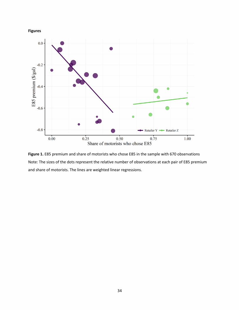
34

Figures

Figure 1. E85 premium and share of motorists who chose E85 in the sample with 670 observations

Note: The sizes of the dots represent the relative number of observations at each pair of E85 premium

and share of motorists. The lines are weighted linear regressions.

35

a) Hypothetical E85 premium and share of motorists who chose E85 at Retailer Y in the sample

with 670 observations

b) Hypothetical E85 premium and share of motorists who chose E85 at Retailer Z in the sample

with 670 observations Figure 2. Hypothetical E85 premium and share of motorists who chose E85 in the sample with 670 observations Note: The sizes of the dots represent the relative number of observations at each pair of E85 premium and share of motorists. The lines are weighted linear regressions.

36

a) Probability of E85 purchase as a function of E85 premium

b) Probability of E85 purchase as a function of E85 ratio

Figure 3. Probability of E85 purchase at Retailer Y estimated with sample of 670 observations

Note: The shaded areas are 95-percent confidence intervals.

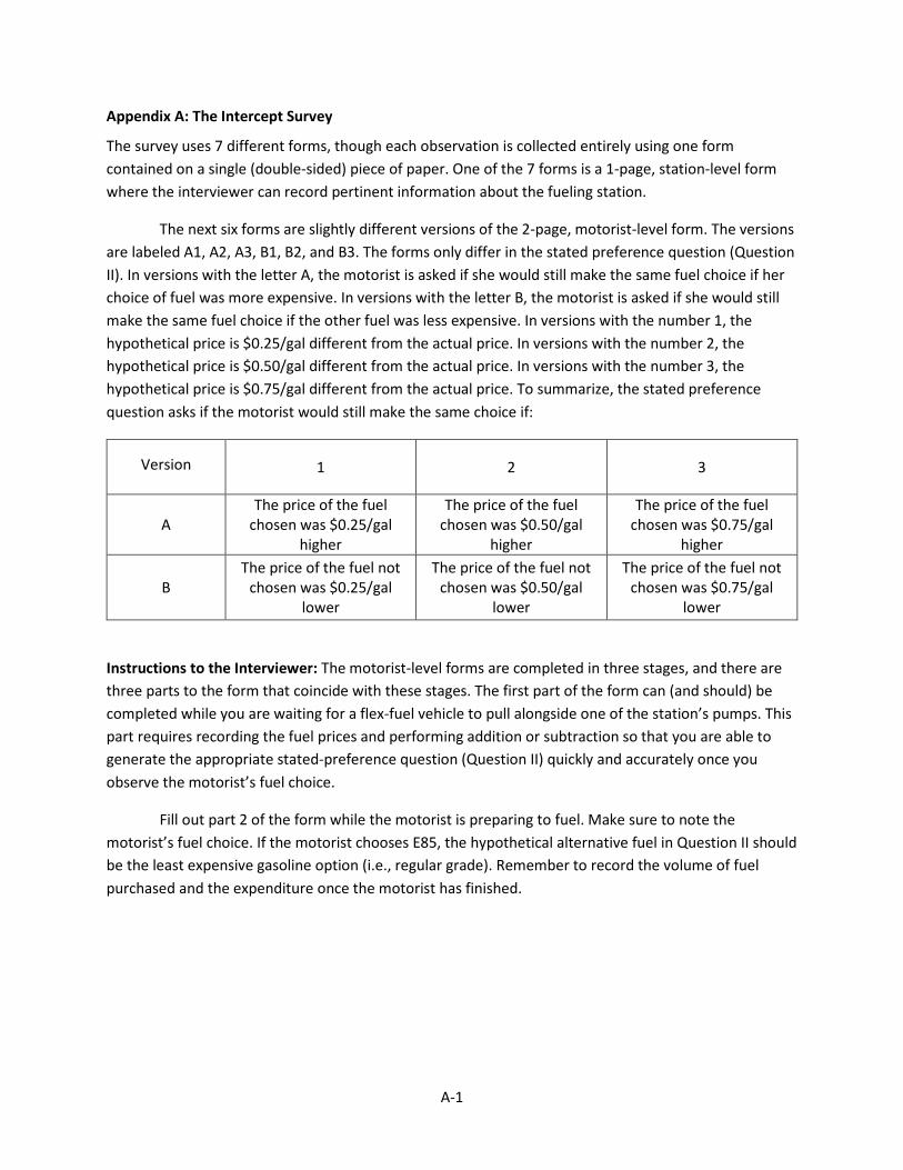
A-1

Appendix A: The Intercept Survey

The survey uses 7 different forms, though each observation is collected entirely using one form contained on a single (double-sided) piece of paper. One of the 7 forms is a 1-page, station-level form where the interviewer can record pertinent information about the fueling station.

The next six forms are slightly different versions of the 2-page, motorist-level form. The versions are labeled A1, A2, A3, B1, B2, and B3. The forms only differ in the stated preference question (Question II). In versions with the letter A, the motorist is asked if she would still make the same fuel choice if her choice of fuel was more expensive. In versions with the letter B, the motorist is asked if she would still make the same fuel choice if the other fuel was less expensive. In versions with the number 1, the hypothetical price is $0.25/gal different from the actual price. In versions with the number 2, the hypothetical price is $0.50/gal different from the actual price. In versions with the number 3, the hypothetical price is $0.75/gal different from the actual price. To summarize, the stated preference question asks if the motorist would still make the same choice if:

Version

1 2 3

A The price of the fuel

chosen was $0.25/gal higher

The price of the fuel chosen was $0.50/gal

higher

The price of the fuel chosen was $0.75/gal

higher

B The price of the fuel not

chosen was $0.25/gal lower

The price of the fuel not chosen was $0.50/gal

lower

The price of the fuel not chosen was $0.75/gal

lower

Instructions to the Interviewer: The motorist-level forms are completed in three stages, and there are three parts to the form that coincide with these stages. The first part of the form can (and should) be completed while you are waiting for a flex-fuel vehicle to pull alongside one of the station’s pumps. This part requires recording the fuel prices and performing addition or subtraction so that you are able to generate the appropriate stated-preference question (Question II) quickly and accurately once you observe the motorist’s fuel choice.

Fill out part 2 of the form while the motorist is preparing to fuel. Make sure to note the motorist’s fuel choice. If the motorist chooses E85, the hypothetical alternative fuel in Question II should be the least expensive gasoline option (i.e., regular grade). Remember to record the volume of fuel purchased and the expenditure once the motorist has finished.

A-2

Survey Form: Station-level

Instructions to the Interviewer: Fill out this form once for each station visit. Answer questions 1-11 upon arriving at the station, and answer question 12 when you conclude the visit.

1. Date and start time of visit: _________________________ 2. Interviewer name: _________________________ 3. Station name and brand: _________________________ 4. Station address: _________________________ 5. Initial per gallon E85 price: _________________________ 6. Gas option 1 – grade, ethanol %, and price: _________________________ 7. Gas option 2 – grade, ethanol %, and price: _________________________ 8. Gas option 3 – grade, ethanol %, and price: _________________________ 9. Number of gasoline nozzles: _________________________ 10. Number of E85 nozzles: _________________________ 11. Presence of E85 price signage _________________________ 12. Date and end time of visit: _________________________

Before You Begin: Each station visit is assigned a 7-digit code for bookkeeping. The code is generated by concatenating today’s date (MMDD) followed by your initials (First, Last) followed by the number of stations you have visited today. For example, if the date is October 15 (1015), your name is Kenneth Liao (KL), and this is the second station you have visited today (2), then the code would be, “1015KL2”.

Write the 7-digit code for this station visit: _________________________

You must write this code on each of the motorist forms you complete during this station visit.

When you are ready to begin, target the next FFV to pull alongside any of the station’s pumps. When you finish one survey, target the next FFV to pull alongside any of the station’s pumps. Do not survey flex motorists who are already at a pump when you arrive, and do not survey flex motorists who pull alongside a pump while you are surveying someone else. There are six versions of the motorist-level form: A1, A2, A3, B1, B2, and B3. Pick one version at random to start, and then proceed to use each version in sequence and repeat.

Write other notes (if any) about the station visit here:

A-3

Survey Form Code: M-A1 Ref/Time:

Part 1: (Fill out this table while waiting for a flex-fuel vehicle to pull alongside one of the station’s pumps.)

E85 Price Gas 1 Price Gas 2 Price

7-digit Station-Visit Code

Actual Prices:

Box 1

Box 2

Box 3

Hypothetical Prices:

(Add $0.25)

(Box 1 + $0.25) 4

(Box 2 + $0.25) 5

(Box 3 + $0.25) 6

Part 2: (Fill out this table while the motorist is preparing to fuel and/or after the motorist has finished.)

Vehicle Type

Vehicle Make

Vehicle Model

LP State

FFV Badge

Yellow Gas Cap

Motorist Sex

Volume & Expenditure

Fuel Choice

Sedan / Truck

SUV / Van Y / N Y / N M / F

E85 / Gas

Part 3: (Fill out this part of the form with assistance from the motorist.)

“Hi, I am doing research for Iowa State University, and I am interested in your opinion on the different fuels. I have a few

short questions to ask you while you are fueling, will you help me by answering?”

“Great! Are you 18 or older?” (If ‘No’ then STOP) (Yes) (No)

I. Is this your personal vehicle? (Yes) (No) ______________

(If company car) Are you: (a) financially responsible for your fuel choice or (b) fully reimbursed regardless?

Only ask these questions if the motorist did NOT choose E85:

a. Is your vehicle a flex-fuel vehicle capable of using E85? (Yes) (No) (Don’t know)

b. (If ‘Yes’ to Q1) Have you ever fueled this vehicle with E85? (Yes) (No) (Don’t know)

c. Did you know that this station supplies E85 fuel? (Yes) (No)

Only ask these questions if the motorist DID choose E85:

d. Did you choose to fuel at this station because it offers E85? (Yes) (No)

e. (If ‘Yes’ to Q4) How far out of your way did you have to drive? (minutes or miles) _____________________

Ask this question to all motorists: (Use the values from Parts 1 and 2 to generate this question.)

II. If the price of (fuel chosen) __________ had been ($0.25/gal more expensive) __________, would you still have purchased (fuel chosen) __________? (Yes) (No)

A-4

Ask these questions to all motorists

III. How many times do you fuel per month? _______________________

IV. (FFVs*) Out of those, how many times do you use E85? _______________________

V. On average, how many miles do you drive per year? _______________________

VI. How old are you? _______________________

“Thanks, we’re almost done. For these last questions, please answer, ‘Ethanol’, ‘Gasoline’, or ‘No Difference’.”

VII. Which fuel is better for the environment? (Eth) (Gas) (ND) (DK)

VIII. Which fuel is better for your engine? (Eth) (Gas) (ND) (DK)

IX. Which fuel is better for the economy? (Eth) (Gas) (ND) (DK)

X. Which fuel is better for national security? (Eth) (Gas) (ND) (DK)

XI. Which fuel yields more miles per gallon? (Eth) (Gas) (ND) (DK)

i. What percentage of the miles per gallon that you get from gas do you get from E85? _____% (DK)

ii. What percentage of the miles per gallon that you get from E85 do you get from gas? _____% (DK)

“Thank you for your participation. Have a nice day.”

B-1

Appendix B: Survey Data and Summary Tables

As described in Section II, we record other observable characteristics about motorists in addition to their

fuel choices before approaching with the intercept survey. The motorists’ characteristics recorded are:

the vehicle make, model, and type (car, truck, SUV, or van), the state on the license plate, whether the

vehicle has an FFV badge, whether the vehicle has a yellow gas cap, and the gender of the motorist.

Table B.1 contains summary statistics for these data. We ended up not using the vehicle license plate

data in our regressions. Instead we use dummy variables for each of the states where we survey. There

was little variation in license plate states within a state so there is near collinearity with the state

dummy variables.

For the vehicle make, the largest share of the vehicles in the sample were Chevrolet, at 46

percent. The most common Chevrolet models were the Silverado, Impala, Tahoe, Suburban, HHR,

Equinox and Malibu. The next most common vehicle make was Ford with 18 percent of the sample and

common models F150, Explorer, Focus, Fusion, and Taurus. Third in our sample was Dodge with 14

percent and common models Grand Caravan, Ram, and Durango. GMC and Chrysler were tied for

fourth, making up 7 percent of our sample each, and the final 8 percent of the sample represented all of

the other vehicle makes.

As for vehicle type, trucks and SUVs each made up about 30 percent of our sample, cars were 25

percent, and vans were the remainder. We were surprised that our sample contained about twice as

many men as women. Our initial expectation was that the population of flex motorists would be about

half men and half women. It is possible that the types of vehicles that tend to be FFVs (large American-

made cars and trucks) are more often driven by men than women. Lastly about 67 percent of the FFVs in

our sample had FFV badges, and about 94 percent had some sort of yellow E85 indicator inside the gas

door. The noteworthy exceptions are the flexible-fuel Toyotas (Tundra and Sequoia) and Nissans (Titan

and Armada), which have badges on the backs, but no yellow gas caps. Other makes and models were

also missing the yellow cap/ring/sticker on rare occasions.

Table B.1 shows that of the 881 flex motorists who completed our survey, 727 (83 percent)

responded that they were refueling their personal FFV. Another 80 motorists (9 percent) were refueling

company FFVs, 27 (3 percent) were refueling government FFVs, and the remaining 47 motorists (5

percent) were refueling other non-personal vehicles like rentals or FFVs that belonged to friends or

family.

B-2

Table B.1: Summary of characteristics of motorists in the sample

Vehicle make Chevrolet 45.9%

Ford 18.2%

Dodge 14.0%

GMC 7.2%

Chrysler 7.2%

Other 7.7% Vehicle type Truck 30.4%

SUV 29.7%

Car 25.5%

Van 14.3% Motorist gender Male 66.4%

Female 33.6% FFV badge Yes 67.0%

No 33.0% Yellow cap/sticker Yes 94.4%

No 5.6% Vehicle ownership (stated) Personal 82.5%

Company 9.1%

Government 3.1% Other 5.3%

Age (stated) Min 18

1st Qu. 33

Median 43

Mean 44.1

3rd Qu. 54 Max 88

Miles per year (stated) Min 500

1st Qu. 12,000 Median 17,000

Mean 21,780 3rd Qu. 27,000 Max 120,000

Summary statistics are for 881 observations of flex motorists refueling at E85 stations in the areas: Little Rock, AR; Los Angeles, CA; Sacramento, CA; Colorado Springs, CO; Ames/Des Moines, IA; and Tulsa, OK. Vehicle type 'Car' includes coupes, convertibles, sedans, hatchbacks, and station wagons.

In the sample, the range of ages span 18 to 88, and the median age is 43. In some cases,

motorists declined to give their age. In these cases the interviewer would move on, and write in an

estimate after the interview was completed. However, we decided to exclude these observations from

the sample along with the other incomplete observations. Similarly, on rare occasions motorists were

unable to answer the question about how intensively they used their vehicle. In most cases, motorists

B-3

were able to offer an approximation of how many miles they drove per year or per month or per week.

Sometimes the motorists would check the odometer and say something like, “Well I’ve driven

[odometer reading] miles in [number of years of car ownership] years.” Most of the cases where the

motorist was unable to answer was when they were not driving their personal vehicle and were unsure

how to respond. Again we excluded these incomplete observations from the sample.

Next, to the motorists who chose E10, we asked questions to measure their knowledge and

awareness of E85. The results are in Table B.2. Of the 450 flex motorists in our sample who refueled

with E10, 385 (86 percent) indicated that they were aware that their vehicle was in fact a flexible-fuel

vehicle capable of using E85. Of the 385 E10 users who were aware of their vehicles’ capabilities, 145

(38 percent) responded that they had refueled with E85 at least once, while the majority had never tried

it. This might be explained by E85 having been historically more expensive than E10 in energy-equivalent

terms. Finally, 280 of the 385 responded that they were aware that the station sold E85, and of the

remaining 105 who answered they did not know, 80 previously responded that they had never used E85.

In general, these are motorists who happen to own FFVs, but know almost nothing about E85. They do

not know what it is, they have never used it, and they certainly do not think to look for it.

Table B.2: Responses to questions to flex motorists who refueled with E10

Yes No / Don't know Total Is your vehicle an FFV? 385 (86%) 65 (14%) 450 Have you ever fueled with E85? 145 (38%) 240 (62%) 385 Did you know this station sells E85? 280 (73%) 105 (27%) 385

We wanted to see if the 450 E10 motorists were responding to the relative fuel prices. To the

motorists who responded that their vehicle was an FFV, we asked the follow-up questions shown.

Between the 65 motorists who did not know their vehicle was an FFV and the 105 motorists who did not

know the station sold E85, there were 170 motorists in our sample who we assume would not have

chosen E85 regardless of the relative prices. Only 145/450 (32 percent) of the flex motorists in our

sample who refueled with E10 had ever refueled with E85.

Out of the 450 flex motorists in our sample who chose E10, 65 did not know they were refueling

an FFV capable of using E85, and another 105 were not aware that the station sold E85. The implication

is that these 170 motorists would not have chosen E85 no matter how low the relative price of E85

would have been. These motorists represent a segment of the population of flex motorists who were

B-4

not aware of the station’s or the vehicle’s capabilities, though they were not necessarily unwilling to use

E85 in the future.

We asked the flex motorists who chose E85 whether they chose to refuel at the station because

of E85, and, if so, how far out of their way they drove. Summary data for these questions are shown in

Table B.3. Out of the 431 motorists who chose E85, 402 (93 percent) said that they chose to refuel at the

station because it offered E85. And out of those 402 motorists, 191 (48 percent) said that they did not

drive out of their way at all. It seems that most motorists drive past a number of fuel stations in their

normal routine, and while they may choose to refuel at a particular station due to the station’s unique

amenities (e.g., whether it offers E85), most motorists do not consider the station they choose to be ‘out

of their way’.21 We use the responses to how far motorists drove to inform about how the general

population of flex motorists differs from our sample population. Specifically, we assume that the

remaining 211 observations of flex motorists who chose E85 and drove out of their way for it are

oversampled. We construct our estimates of the population shares by removing those 211 observations

from our sample.

Table B.3: Responses to questions to flex motorists who refueled with E85

Did you choose to fuel at this station because it offers E85? Yes 402 (93.3%)

No 29 (6.7%)

Total 436 How far out of your way did you drive? (miles) Not at all (zero mi.) 191 (47.5%)

(0,1] miles 44 (10.9%) (1,3] miles 73 (18.2%)

(3,5] miles 42 (10.4%) (5,10] miles 38 (9.5%) More than 10 miles 14 (3.5%)

Total 402 Statistics are for the 431 observations of flex motorists in our sample who chose to refuel with E85. In

total, 402/431 (93%) said they came for the E85, but of those 402 motorists, 191 said that they did not

drive out of their way at all. We remove the remaining 211 motorists who drove out of their way for E85

from the sample to create a sample that is more representative of the population.

21 In retrospect, a better way to ask this question may have been something along the lines of, “If every gas station

in the area offered E85, would you still have chosen to refuel at this station?”

B-5

Responses to the questions we have discussed to this point do not differ significantly by

state/region. The measurable differences in the data across regions are in the fuel prices and observed

choices, as shown in Table 1, but also in the fuel opinion questions shown in Table B.4 and Table B.5.

Table B.4 shows the responses to the fuel opinion questions by region from only the 450 motorists who

refueled with E10, and Table B.5 shows the responses from only the 431 motorists who chose E85. In

the three questions about which fuel is better for the environment, the engine, and the economy, the

differences in opinions across regions are especially apparent. In general, a greater share of flex

motorists we surveyed in Iowa and California believe that ethanol is better for the environment, for a

vehicle’s engine, and for the economy, while the average motorist in Arkansas and Oklahoma has a

much less favorable opinion of ethanol in these same areas, and the average motorist in Colorado is

somewhere in between.

We separate the responses by fuel choice so we can compare the opinions across regions

separately from fuel choices across regions. Table B.4 shows that even among only the motorists who

choose E10, motorists have a much higher opinion of ethanol in Iowa than they do elsewhere when it

comes to the environment and the economy, and the other factors. In Iowa, 78 percent of E10-using flex

motorists responded that ethanol was better for the environment, and 71 percent responded that

ethanol was better for the economy. On the other hand, in Oklahoma, 42 percent of E10-using flex

motorists responded that ethanol was better for the environment, and 25 percent responded that

ethanol was better for the economy. Note that of the 231 observations we collected at Retailer Z’s

California locations, only 26 chose E10. Also note that we collected fuel opinion data for all of the flex

motorists in our sample, even those who did not know they had an FFV or did not know anything about

ethanol or E85.

Table B.6 likewise shows that even among only the motorists in our sample who chose E85,

average opinions of ethanol are much higher in Iowa and California than in Arkansas, Colorado, and

Oklahoma. At the extremes are Iowa and Oklahoma. Among the flex motorists who chose to refuel with

E85, 84 percent in Iowa responded that ethanol was better for the environment, compared to 43

percent in Oklahoma. And 87 percent of E85-using Iowa motorists responded that ethanol was better

for the economy compared to 55 percent in Oklahoma. We model the opinions as explanatory variables

in our empirical model. The opinions are especially informative when we compare the Iowa data with

the data from Arkansas and Oklahoma. Retailer Y operated all the stations in these regions and the

E85/E10 price ratios were quite similar. By contrast, opinions of ethanol were drastically different.

B-6

Table B.4: Responses to fuel opinion questions by region from flex motorists who refueled with E10

Region Observations Ethanol Gasoline No difference

Don't know

Which fuel is better for the environment?

Little Rock 73 52% 18% 14% 16% Los Angeles 12 50% 25% 8% 17% Sacramento 14 64% 7% 7% 21% Colorado Springs 80 64% 5% 13% 19%

Ames/Des Moines 180 77% 6% 11% 6% Tulsa 91 42% 19% 25% 14%

Total 450 62% 11% 14% 12%

Which fuel is better for your engine?

Little Rock 73 18% 52% 14% 16% Los Angeles 12 0% 42% 25% 33% Sacramento 14 14% 43% 7% 36% Colorado Springs 80 24% 48% 15% 14%

Ames/Des Moines 180 25% 42% 18% 14% Tulsa 91 13% 69% 9% 9% Total 450 20% 50% 15% 15%

Which fuel is better for the economy?

Little Rock 73 33% 45% 4% 18% Los Angeles 12 25% 50% 0% 25% Sacramento 14 43% 14% 14% 29% Colorado Springs 80 44% 30% 11% 15%

Ames/Des Moines 180 71% 12% 10% 8%

Tulsa 91 25% 44% 15% 15%

Total 450 48% 28% 10% 13%

Which fuel is better for national security?

Little Rock 73 32% 29% 12% 27% Los Angeles 12 25% 33% 0% 42% Sacramento 14 21% 21% 14% 43% Colorado Springs 80 34% 31% 24% 11% Ames/Des Moines 180 51% 13% 11% 25%

Tulsa 91 21% 29% 30% 21%

Total 450 37% 23% 17% 23%

Which fuel yields more miles per gallon?

Little Rock 73 12% 66% 7% 15% Los Angeles 12 8% 50% 0% 42% Sacramento 14 7% 50% 0% 43% Colorado Springs 80 16% 60% 5% 19% Ames/Des Moines 180 8% 76% 4% 12%

Tulsa 91 10% 67% 3% 20%

Total 450 10% 68% 4% 17% Summary statistics are for survey data collected from 450 flex motorists who refueled with E10.

B-7

Table B.5: Responses to fuel opinion questions by region from flex motorists who refueled with E85

Region Observations Ethanol Gasoline No difference

Don't know

Which fuel is better for the environment?

Little Rock 36 67% 6% 19% 8% Los Angeles 125 82% 0% 6% 13% Sacramento 80 85% 0% 9% 6% Colorado Springs 18 67% 6% 11% 17%

Ames/Des Moines 128 84% 1% 11% 5% Tulsa 44 43% 9% 30% 18%

Total 431 77% 2% 12% 10%

Which fuel is better for your engine?

Little Rock 36 44% 28% 17% 11% Los Angeles 125 64% 8% 10% 18% Sacramento 80 55% 14% 21% 10% Colorado Springs 18 39% 33% 6% 22%

Ames/Des Moines 128 41% 31% 17% 10% Tulsa 44 32% 34% 16% 18% Total 431 50% 21% 15% 14%

Which fuel is better for the economy?

Little Rock 36 56% 19% 17% 8% Los Angeles 125 78% 8% 6% 8% Sacramento 80 66% 18% 10% 6% Colorado Springs 18 44% 33% 17% 6%

Ames/Des Moines 128 88% 4% 4% 5%

Tulsa 44 55% 20% 16% 9%

Total 431 73% 12% 9% 7%

Which fuel is better for national security?

Little Rock 36 44% 28% 11% 17% Los Angeles 125 45% 10% 6% 39% Sacramento 80 44% 6% 15% 35% Colorado Springs 18 28% 11% 28% 33% Ames/Des Moines 128 70% 7% 5% 17%

Tulsa 44 30% 23% 20% 27%

Total 431 50% 11% 10% 29%

Which fuel yields more miles per gallon?

Little Rock 36 28% 56% 8% 8% Los Angeles 125 30% 40% 14% 16% Sacramento 80 15% 55% 18% 13% Colorado Springs 18 17% 61% 6% 17% Ames/Des Moines 128 20% 66% 5% 10%

Tulsa 44 23% 52% 5% 20%

Total 431 23% 54% 10% 13% Summary statistics are for survey data collected from 431 flex motorists who refueled with E85.

B-8

For some of the flex motorists we surveyed, the question about national security elicited more

confusion rather than an actual response. In 2006, national security and independence from foreign oil

were touted as reasons to support the biofuels mandates, but the cause seems to have lost importance

with flex motorists in 2015. As with the other questions, motorists in Iowa and California favor ethanol

more than the motorists in the other urban areas, but there were also many more cases where the

motorists answered, “No difference” or, “Don’t know”.

The last question of the survey asked which fuel yields more miles per gallon. In Iowa, about 67

percent of the flex motorists correctly answered E10 yielded more miles per gallon than E85. About 19

percent said that E85 yielded more miles per gallon than E10, 5 percent said there was no difference,

and 10 percent answered that they did not know. In other regions, the percentage of motorists who

correctly identify that E10 yielded more miles per gallon was even lower. In Colorado Springs, 61

percent answered correctly, and in Little Rock, Sacramento, and Tulsa, 56 percent, 55 percent, and 52

percent of motorists respectively correctly answered. Finally, in Los Angeles, just 40 percent of the flex

motorists we surveyed responded that E10 yields more miles per gallon, 30 percent said E85 was better,

14 percent said there was no difference, and 16 percent answered that they did not know. Ignorance

about the energy difference of the two fuels likely explains why some motorists drive miles out of their

way or wait in line to refuel with E85. We also asked the motorists a follow up question to approximate

the percentage the relative energy difference between the two fuels. Some motorists responded with

an accurate answer saying that E85 gets about 75-80 percent of the miles per gallon of E10. Some

approximated higher energy for E85 in the 90 percent range and some approximated the energy ratio to

be as low as 50 percent. Responses were not always in the form of a simple percentage of energy

content, but rather some motorists knew the miles per gallon of each, “I get 14 mpg with E85 and 18

mpg with E10,” and others knew how long a tank of each of the two fuels lasted.

Interestingly, many of the flex motorists who chose E85 demonstrated that they understood

that E85 was more expensive on an energy-equivalent basis. Some chose E85 for reasons other than the

price, while others simply did not bother to calculate the energy-equivalent fuel costs every time they

filled up. Many flex motorists said something along the lines of, “I did the math once and figured that I

need a $0.60 per gallon discount on E85 for it to be worth it,” and now they make their fuel choice

based on some rule-of-thumb or routine.

C-1

Appendix C: Complete Estimation Results

Table C.1. Marginal effects for E85 premium models: Model 1-A through Model 1-E

Model 1-A Model 1-B Model 1-C Model 1-D Model 1-E

Marg.

Eff. SE Marg.

Eff. SE Marg.

Eff. SE Marg.

Eff. SE Marg.

Eff. SE PREM -0.117 0.063 -0.146 0.096 -0.121 0.054 -0.113 0.034 -0.151 0.055 GOV 0.108 0.058 0.152 0.088 0.111 0.059 0.108 0.069 0.158 0.106 COMP -0.056 0.039 -0.062 0.060 -0.039 0.034 -0.039 0.029 -0.041 0.046 ONPV 0.039 0.034 0.056 0.052 0.020 0.041 0.007 0.041 0.026 0.064 VTYPE_TRUCK -0.008 0.028 -0.012 0.044 -0.012 0.028 -0.003 0.021 -0.007 0.033 VTYPE_SUV -0.007 0.027 -0.012 0.043 -0.016 0.028 -0.010 0.022 -0.015 0.035 VTYPE_VAN 0.020 0.029 0.025 0.045 0.012 0.040 0.003 0.031 0.003 0.049 BADGE -0.029 0.020 -0.039 0.031 -0.009 0.025 0.006 0.020 0.005 0.032 FEMALE 0.008 0.022 0.011 0.035 -0.021 0.031 -0.034 0.024 -0.042 0.039 AGE -0.001 0.001 -0.001 0.001 -0.001 0.001 0.000 0.001 0.000 0.001 TMPY -0.001 0.001 -0.001 0.001 -0.002 0.001 -0.001 0.001 -0.002 0.001 ENV_ETH -0.019 0.040 -0.035 0.063 -0.020 0.044 -0.013 0.034 -0.031 0.053 ENV_GAS -0.081 0.059 -0.094 0.091 -0.140 0.091 -0.102 0.056 -0.108 0.085 ENV_ND -0.100 0.058 -0.127 0.089 -0.120 0.063 -0.086 0.043 -0.115 0.066 ENG_ETH 0.078 0.038 0.089 0.058 0.063 0.040 0.055 0.035 0.062 0.054 ENG_GAS 0.047 0.039 0.049 0.060 0.036 0.042 0.025 0.032 0.020 0.051 ENG_ND -0.019 0.057 -0.013 0.089 -0.001 0.047 0.014 0.034 0.010 0.054 ECON_ETH 0.086 0.053 0.089 0.081 0.103 0.059 0.092 0.045 0.096 0.069 ECON_GAS 0.024 0.056 0.014 0.087 0.049 0.059 0.056 0.045 0.052 0.071 ECON_ND 0.132 0.058 0.150 0.087 0.130 0.064 0.098 0.051 0.106 0.078 NS_ETH 0.013 0.025 0.013 0.040 0.025 0.029 0.017 0.025 0.019 0.040 NS_GAS 0.042 0.031 0.048 0.047 0.048 0.035 0.036 0.030 0.045 0.047 NS_ND -0.050 0.041 -0.061 0.065 -0.002 0.039 0.019 0.027 0.023 0.042 MPG_ETH 0.008 0.038 0.010 0.060 -0.004 0.044 -0.029 0.041 -0.032 0.064 MPG_GAS 0.036 0.033 0.039 0.052 0.036 0.036 0.014 0.027 0.013 0.043 MPG_ND 0.067 0.053 0.093 0.084 0.101 0.041 0.077 0.033 0.105 0.051 STNST_AR 0.031 0.036 0.041 0.056 0.035 0.029 0.019 0.026 0.028 0.041 STNST_CO 0.048 0.046 0.067 0.072 0.041 0.041 0.030 0.030 0.050 0.049 STNST_OK 0.066 0.036 0.087 0.056 0.060 0.033 0.048 0.024 0.067 0.038 STNST_CA 0.125 0.028 0.155 0.041 0.116 0.030 0.105 0.030 0.136 0.044

Sample size is 479 observations using the strictest sample-selection rule. All dummies equal zero is: personal vehicle, car type, no FFV badge, male, and “don’t know” to all opinion questions.

C-2

Table C.2. Marginal effects for E85 ratio models: Model 2-A through Model 2-E Model 2-A Model 2-B Model 2-C Model 2-D Model 2-E

Marg.

Eff. SE Marg.

Eff. SE Marg.

Eff. SE Marg.

Eff. SE Marg.

Eff. SE LOG_RATIO -0.342 0.170 -0.424 0.257 -0.264 0.105 -0.247 0.059 -0.341 0.099 GOV 0.111 0.058 0.156 0.088 0.125 0.053 0.096 0.072 0.153 0.114 COMP -0.061 0.039 -0.067 0.060 -0.039 0.032 -0.034 0.027 -0.037 0.043 ONPV 0.038 0.033 0.055 0.052 0.011 0.038 0.001 0.038 0.018 0.062 VTYPE_TRUCK -0.009 0.028 -0.014 0.044 -0.020 0.023 -0.019 0.020 -0.028 0.032 VTYPE_SUV -0.007 0.028 -0.011 0.043 -0.018 0.024 -0.017 0.020 -0.025 0.033 VTYPE_VAN 0.019 0.029 0.024 0.045 -0.006 0.033 -0.011 0.029 -0.015 0.047 BADGE -0.030 0.020 -0.039 0.031 -0.007 0.023 0.011 0.019 0.010 0.031 FEMALE 0.009 0.022 0.013 0.035 -0.028 0.026 -0.035 0.022 -0.045 0.036 AGE -0.034 0.030 -0.043 0.046 -0.042 0.029 -0.026 0.025 -0.035 0.040 TMPY -0.019 0.017 -0.022 0.027 -0.026 0.012 -0.011 0.011 -0.015 0.018 ENV_ETH -0.017 0.040 -0.032 0.062 0.023 0.049 0.012 0.033 -0.002 0.055 ENV_GAS -0.082 0.059 -0.095 0.090 -0.071 0.069 -0.079 0.054 -0.069 0.085 ENV_ND -0.098 0.058 -0.124 0.088 -0.056 0.057 -0.054 0.040 -0.077 0.065 ENG_ETH 0.080 0.038 0.091 0.059 0.085 0.049 0.068 0.039 0.080 0.062 ENG_GAS 0.049 0.039 0.050 0.061 0.058 0.050 0.043 0.035 0.043 0.057 ENG_ND -0.016 0.057 -0.010 0.089 0.040 0.048 0.036 0.036 0.040 0.059 ECON_ETH 0.084 0.053 0.086 0.080 0.073 0.052 0.048 0.033 0.048 0.052 ECON_GAS 0.025 0.056 0.015 0.086 0.027 0.053 0.012 0.035 0.002 0.057 ECON_ND 0.132 0.057 0.150 0.086 0.089 0.058 0.051 0.039 0.057 0.062 NS_ETH 0.014 0.026 0.013 0.040 0.018 0.026 0.007 0.023 0.005 0.037 NS_GAS 0.040 0.031 0.046 0.047 0.037 0.032 0.023 0.028 0.030 0.044 NS_ND -0.053 0.042 -0.064 0.065 -0.003 0.036 0.001 0.027 0.001 0.043 MPG_ETH 0.009 0.039 0.010 0.061 -0.008 0.038 -0.003 0.039 -0.003 0.063 MPG_GAS 0.036 0.033 0.039 0.052 0.025 0.031 0.021 0.027 0.020 0.044 MPG_ND 0.059 0.052 0.080 0.082 0.078 0.038 0.077 0.033 0.107 0.052 STNST_AR 0.025 0.034 0.033 0.054 0.013 0.029 0.001 0.028 0.006 0.045 STNST_CO 0.055 0.048 0.074 0.074 0.021 0.033 0.025 0.025 0.041 0.042 STNST_OK 0.062 0.035 0.081 0.053 0.040 0.029 0.029 0.024 0.044 0.039 STNST_CA 0.134 0.029 0.166 0.042 0.116 0.031 0.101 0.027 0.136 0.041

Sample size is 479 observations using the strictest sample-selection rule. All dummies equal zero is: personal vehicle, car type, no FFV badge, male, and “don’t know” to all opinion questions.

C-3

Table C.3. Marginal effects for E85 premium models: Model 3-A through Model 1-E Model 3-A Model 3-B Model 3-C Model 3-D Model 3-E

Marg.

Eff. SE Marg.

Eff. SE Marg.

Eff. SE Marg.

Eff. SE Marg.

Eff. SE PREM -0.246 0.080 -0.246 0.084 -0.078 0.047 -0.294 0.021 -0.296 0.022 GOV 0.388 0.078 0.374 0.083 0.489 0.082 0.463 0.095 0.443 0.101 COMP -0.028 0.051 -0.027 0.054 0.011 0.047 -0.010 0.049 -0.008 0.052 ONPV -0.020 0.067 -0.014 0.071 -0.062 0.067 -0.043 0.069 -0.035 0.073 VTYPE_TRUCK 0.040 0.038 0.038 0.040 0.025 0.035 0.018 0.033 0.016 0.035 VTYPE_SUV -0.054 0.040 -0.053 0.042 -0.067 0.036 -0.039 0.034 -0.040 0.036 VTYPE_VAN -0.038 0.048 -0.037 0.050 -0.055 0.049 -0.057 0.048 -0.056 0.051 BADGE 0.033 0.031 0.033 0.033 0.073 0.030 0.073 0.029 0.072 0.030 FEMALE 0.039 0.033 0.039 0.035 0.036 0.031 0.006 0.032 0.006 0.034 AGE 0.001 0.001 0.001 0.001 0.000 0.001 0.000 0.001 0.000 0.001 TMPY -0.001 0.001 -0.001 0.001 -0.002 0.001 -0.001 0.001 -0.001 0.001 ENV_ETH -0.026 0.053 -0.027 0.057 -0.016 0.049 -0.010 0.046 -0.011 0.048 ENV_GAS -0.142 0.085 -0.135 0.090 -0.150 0.083 -0.156 0.081 -0.145 0.085 ENV_ND -0.038 0.064 -0.037 0.068 -0.015 0.057 -0.044 0.058 -0.043 0.061 ENG_ETH 0.132 0.046 0.131 0.048 0.162 0.045 0.115 0.044 0.115 0.046 ENG_GAS -0.042 0.048 -0.043 0.050 -0.010 0.049 -0.025 0.044 -0.026 0.046 ENG_ND 0.039 0.052 0.039 0.055 0.074 0.049 0.046 0.046 0.045 0.049 ECON_ETH 0.163 0.055 0.160 0.058 0.174 0.055 0.150 0.051 0.147 0.054 ECON_GAS 0.020 0.065 0.019 0.069 0.056 0.062 0.041 0.057 0.039 0.061 ECON_ND 0.144 0.070 0.143 0.074 0.109 0.068 0.070 0.062 0.069 0.065 NS_ETH 0.034 0.037 0.032 0.039 0.054 0.035 0.040 0.035 0.038 0.037 NS_GAS 0.047 0.051 0.046 0.054 0.036 0.052 0.026 0.047 0.025 0.050 NS_ND -0.029 0.053 -0.029 0.056 0.023 0.048 0.034 0.041 0.034 0.044 MPG_ETH 0.039 0.055 0.039 0.058 0.031 0.052 0.009 0.054 0.009 0.057 MPG_GAS 0.096 0.044 0.094 0.047 0.094 0.044 0.064 0.043 0.062 0.046 MPG_ND 0.158 0.069 0.158 0.073 0.160 0.060 0.113 0.053 0.113 0.056 STNST_AR 0.029 0.047 0.030 0.050 0.005 0.045 0.028 0.046 0.030 0.049 STNST_CO 0.019 0.064 0.024 0.068 -0.061 0.051 0.033 0.048 0.038 0.050 STNST_OK 0.107 0.048 0.107 0.051 0.061 0.042 0.095 0.039 0.096 0.042 STNST_CA 0.400 0.035 0.394 0.037 0.399 0.032 0.319 0.029 0.315 0.031

C-4

Table C.4: Marginal effects for E85 ratio Models 4 Model 4-A Model 4-B Model 4-C Model 4-D Model 4-E

Marg.

Eff. SE Marg.

Eff. SE Marg.

Eff. SE Marg.

Eff. SE Marg.

Eff. SE Log(ratio) -0.681 0.212 -0.681 0.224 -0.394 0.195 -0.602 0.059 -0.604 0.062 GOV 0.387 0.078 0.372 0.083 -0.210 0.114 0.469 0.106 0.448 0.113 COMP -0.033 0.050 -0.032 0.053 0.450 0.082 -0.020 0.049 -0.019 0.051 ONPV -0.022 0.067 -0.015 0.071 -0.024 0.050 -0.061 0.072 -0.052 0.076 VTYPE_TRUCK 0.040 0.038 0.039 0.040 -0.048 0.065 0.015 0.034 0.014 0.036 VTYPE_SUV -0.052 0.040 -0.052 0.042 0.013 0.036 -0.048 0.034 -0.048 0.036 VTYPE_VAN -0.036 0.048 -0.036 0.051 -0.076 0.036 -0.050 0.048 -0.050 0.051 BADGE 0.034 0.031 0.034 0.032 -0.066 0.049 0.064 0.029 0.064 0.030 FEMALE 0.039 0.034 0.039 0.035 0.055 0.030 0.013 0.033 0.013 0.035 AGE 0.049 0.043 0.049 0.046 0.029 0.031 0.008 0.042 0.008 0.045 TMPY -0.025 0.023 -0.025 0.024 0.004 0.042 -0.014 0.020 -0.013 0.021 ENV_ETH -0.023 0.053 -0.024 0.056 -0.022 0.020 -0.015 0.045 -0.016 0.048 ENV_GAS -0.141 0.085 -0.133 0.090 -0.036 0.046 -0.172 0.084 -0.158 0.089 ENV_ND -0.038 0.064 -0.037 0.067 -0.216 0.095 -0.035 0.057 -0.035 0.060 ENG_ETH 0.129 0.046 0.128 0.048 -0.040 0.055 0.109 0.043 0.108 0.046 ENG_GAS -0.045 0.048 -0.046 0.050 0.134 0.044 -0.045 0.043 -0.046 0.046 ENG_ND 0.038 0.052 0.037 0.055 -0.038 0.048 0.032 0.046 0.032 0.048 ECON_ETH 0.162 0.055 0.159 0.058 0.054 0.049 0.150 0.050 0.148 0.053 ECON_GAS 0.022 0.065 0.020 0.069 0.174 0.053 0.043 0.057 0.042 0.060 ECON_ND 0.145 0.070 0.143 0.074 0.055 0.060 0.083 0.061 0.082 0.065 NS_ETH 0.035 0.037 0.034 0.039 0.122 0.067 0.036 0.034 0.035 0.036 NS_GAS 0.046 0.051 0.045 0.054 0.033 0.035 0.027 0.048 0.026 0.051 NS_ND -0.028 0.053 -0.028 0.056 0.006 0.052 0.024 0.042 0.024 0.045 MPG_ETH 0.037 0.055 0.037 0.058 -0.017 0.049 -0.004 0.054 -0.003 0.057 MPG_GAS 0.095 0.044 0.093 0.047 0.019 0.052 0.058 0.042 0.056 0.045 MPG_ND 0.157 0.069 0.156 0.073 0.071 0.043 0.113 0.052 0.114 0.055 STNST_AR 0.010 0.046 0.011 0.049 0.110 0.060 -0.020 0.048 -0.019 0.051 STNST_CO 0.026 0.065 0.031 0.069 -0.016 0.047 -0.015 0.050 -0.009 0.053 STNST_OK 0.091 0.046 0.091 0.049 -0.063 0.051 0.049 0.041 0.050 0.043 STNST_CA 0.414 0.034 0.408 0.036 0.059 0.042 0.324 0.030 0.320 0.032