estimating willingness to pay for improvements in mobile
TRANSCRIPT

Estimating Willingness to Pay for Improvements in
Mobile Services
Orhan Dağlı
Submitted to the
Institute of Graduate Studies and Research
in partial fulfilment of the requirements for the degree of
Doctor of Philosophy
in
Economics
Eastern Mediterranean University
May 2016
Gazimağusa, North Cyprus

Approval of the Institute of Graduate Studies and Research
__________________________
Prof. Dr. Cem Tanova
Acting Director
I certify that this thesis satisfies the requirements as a thesis for the degree of Doctor
of Philosophy in Economics.
____________________________
Prof. Dr. Mehmet Balcılar
Chair, Department of Economics
We certify that we have read this thesis and that in our opinion it is fully adequate in
scope and quality as a thesis for the degree of Doctor of Philosophy in Economics.
__________________________
Prof. Dr. Glenn P. Jenkins
Supervisor
Examining Committee
1. Prof. Dr. Mehmet Balcılar _________________________________
2. Prof. Dr. Murat Çokgezen _________________________________
3. Prof. Dr. Glenn P. Jenkins _________________________________
4. Prof. Dr. Arman T. Tevfik _________________________________
5. Asst. Prof. Dr. Kemal Bağzıbağlı _________________________________

iii
ABSTRACT
The prominent approach for estimating people’s willingness to pay (WTP) for goods
or services not currently in the market is the stated preference approach. Two methods
of measuring stated WTP are contingent valuation method and choice experiments.
We employ both methods in order to estimate consumers’ valuation of improvements
in mobile services, focusing on 4G upgrades and roaming services. The contingent
valuation method is performed in the payment ladder format, in order to estimate a
nominal WTP for 4G. The choice experiment splits up the “mobile service
improvement” into attributes, and investigates the preferences for these individual
attributes: increased mobile internet speed (possible with 4G), unlimited mobile
internet use, improved quality (possible with 4G) and unrestrained use in two
neighbouring countries (unrestrained roaming). We collect the data for the study
through a face-to-face survey held in all districts of North Cyprus. The results indicate
that people value unrestrained roaming services the most. Increased speed and
unlimited use attributes are next, and are similarly significant at the 1% level. The
impact of improved quality is statistically insignificant at the 5% level, suggesting that
consumers are content with the current level of quality they receive with 3G. We
conclude that bilateral roaming regulation between governments is more valuable than
4G investments.
Keywords: Mobile telecommunication services, Choice experiment, Willingness to
pay, 4G, Roaming.

iv
ÖZ
Hâlihazırda pazarda olmayan ürün veya hizmetler için halkın ödeme istekliliğini (Öİ)
tespit etmek adına kullanılan başlıca yaklaşım bahsedilen tercih yaklaşımıdır.
Bahsedilen Öİ değerini ölçmenin iki yöntemi olası değerlendirme yöntemi ve seçim
deneyleridir. Bu çalışmada tüketicilerin mobil hizmetlerdeki (4G ve dolaşım odaklı)
iyileştirmelere biçtiği ekonomik değeri ölçmek için iki yöntemi de kullandık. Olası
değerlendirme yöntemi ödeme merdiveni formatında, 4G için ödeme istekliliği
değerini tespit etmek adına uygulanmıştır. Seçim deneyi yöntemi mobil hizmet
iyileştirmesini parçalarına ayırıp bu parçalar ile ilgili tercihleri tespit etmek amaçlı
kullanılmıştır. Bu parçalar mobil internet hızında artış (4G ile mümkün), sınırsız mobil
internet kullanımı, iyileşmiş kalite (4G ile mümkün) ve iki komşu ülkede engelsiz
kullanımdır (engelsiz dolaşım). Çalışmada kullanılan veri Kuzey Kıbrıs’ın tüm
ilçelerinde, yüz yüze mülakat yöntemi ile yapılan bir anket ile elde edilmiştir. Sonuçlar
insanların en fazla engelsiz dolaşım hizmetlerine değer verdiğini göstermektedir.
Ardından sırasıyla internet hızında artış ve sınırsız kullanım gelmektedir, ve bu iki
özelliğin etkileri %1 derecesinde anlamlıdır. İyileştirilmiş kalitenin etkisi %5
derecesinde anlamsızdır, bu da tüketicilerin 3G ile sahip oldukları mevcut kalite
seviyesinden memnun olduğunu göstermektedir. Buradan da çift taraflı dolaşım
düzenlemelerinin 4G yatırımlarından daha değerli olduğu sonucuna varıyoruz.
Anahtar kelimeler: Mobil telekomünikasyon hizmetleri, Seçim deneyi, Ödeme
İstekliliği, 4G, Roaming.

v
To My Wife & My Son
vi
ACKNOWLEDGEMENT
I am grateful to my supervisor, Prof. Dr. Glenn P. Jenkins, whose expertise,
understanding, generous guidance and support made it possible for me to produce this
study. It is a pleasure working with him.
I would also like to thank all the faculty members of the Department of Economics at
Eastern Mediterranean University. Their contribution to my learning is vast, and their
teaching has made my EMU years enjoyable.

vii
TABLE OF CONTENTS
ABSTRACT ................................................................................................................ iii
ÖZ ............................................................................................................................... iv
DEDICATION ............................................................................................................. v
ACKNOWLEDGEMENT .......................................................................................... vi
LIST OF TABLES ....................................................................................................... x
LIST OF FIGURES .................................................................................................... xi
1 INTRODUCTION .................................................................................................... 1
1.1 Introduction ......................................................................................................... 1
1.2 Mobile Communications ..................................................................................... 2
1.3 MC Improvements .............................................................................................. 3
1.4 Dissertation Outline ............................................................................................ 5
2 LITERATURE REVIEW.......................................................................................... 7
2.1 Introduction ......................................................................................................... 7
2.2 Willingness-To-Pay or Willingness-To-Accept? ................................................ 8
2.3 Revealed Preference Approach ......................................................................... 10
2.3.1 Averting Expenditure ............................................................................... 10
2.4 Stated Preference Approach .............................................................................. 13
2.4.1 Contingent Valuation Methodology ......................................................... 13
2.4.1.1 Theory behind the CVM Method ................................................. 15
2.4.1.2 Random Utility Approach in CVM .............................................. 15
2.4.1.3 Parametric Modelling of the WTP in CVM ................................. 19
2.4.1.4 Non-Parametric Modelling of the WTP in CVM ......................... 21
2.4.2 Choice Experiments Methodology ........................................................... 21

viii
2.4.2.1 Theory behind the CE Methodology ............................................ 23
2.4.3 Review of Selected Consumer Studies on the Value of Broadband Services
.(Fixed & Mobile) .............................................................................................. 28
2.4.3.1 Consumer Studies for Fixed Broadband Services ........................ 28
2.4.3.2 Consumer Studies for Mobile Broadband Services ..................... 30
3 CHOICE EXPERIMENT DESIGN ........................................................................ 33
3.1 Introduction ....................................................................................................... 33
3.2 Problem Refinement ......................................................................................... 34
3.3 Stimuli Refinement ........................................................................................... 35
3.4 Experimental Design Consideration ................................................................. 39
3.5 Generating Experimental Design ...................................................................... 41
3.6 Allocating Attributes to Design Columns ......................................................... 43
3.7 Generating Choice Sets ..................................................................................... 46
3.8 Versions of Choice Sets .................................................................................... 55
3.9 Randomizing Choice Sets ................................................................................. 56
3.10 Constructing the Survey Instrument ............................................................... 57
4 SURVEY DESIGN AND ADMINISTRATION .................................................... 59
4.1 Introduction ....................................................................................................... 59
4.2 Survey Sections ................................................................................................. 59
4.3 Sample Size ....................................................................................................... 61
4.4 Sampling Method .............................................................................................. 62
4.5 Questionnaire Results........................................................................................ 63
5 CHOICE EXPERIMENT RESULTS ..................................................................... 67
5.1 Revisiting the CE Model ................................................................................... 67
5.2 Estimating the Model ........................................................................................ 69
ix
5.3 Results ............................................................................................................... 70
5.3.1 The Goodness of Fit of the Model ........................................................... 70
5.3.2 Results of MNL Estimation ..................................................................... 70
6 CVM RESULTS ..................................................................................................... 74
6.1 Introduction ....................................................................................................... 74
6.2 Data ................................................................................................................... 76
6.3 Turnbull Lower Bound Mean for WTP ............................................................ 77
6.4 Kriström Mean .................................................................................................. 79
6.5 Upper Bound Mean ........................................................................................... 80
6.6 Sensitivity Analysis ........................................................................................... 80
6.7 Revenue and Consumer Surplus ....................................................................... 82
7 CONCLUSION ....................................................................................................... 86
7.1 Discussion and Conclusion ............................................................................... 86
REFERENCES ........................................................................................................... 93
APPENDICES ......................................................................................................... 103
Appendix A: Experiment Design Tables .............................................................. 104
Appendix B: Survey Questionnaire ...................................................................... 116
x
LIST OF TABLES
Table 3.1: List of Attributes ....................................................................................... 36
Table 3.2: Final List of Attributes and Attribute Levels ............................................ 38
Table 3.3: Final List of Attributes with Design Coding ............................................ 41
Table 3.4: Orthogonal Design Generated with 32 Profiles ........................................ 42
Table 3.5: Orthogonal Plan with Columns Labelled .................................................. 45
Table 3.6: Profiles for Service A Sorted by Blocking Variable ................................. 46
Table 3.7: Final Version of Service A and Service B in Design Codes .................... 50
Table 3.8: Final Version of Service A and Service B with Labelled Attribute Levels
.................................................................................................................................... 51
Table 3.9: Versions of the Choice Experiment .......................................................... 55
Table 3.10: Complete List of Randomized CE Versions ........................................... 56
Table 3.11: A Sample Choice Set .............................................................................. 58
Table 4.1: ESRS Sampling according to Districts ..................................................... 63
Table 4.2: Questionnaire Results ............................................................................... 64
Table 5.1: Results of MNL Model Estimation ........................................................... 71
Table 5.2: MWTP for the Attributes .......................................................................... 72
Table 6.1: Reasons for Zero WTP.............................................................................. 76
Table 6.2: Frequencies of Ticks and Crosses ............................................................. 76
Table 6.3: Cumulative Number and Proportion of Ticks ........................................... 77
Table 6.4: Calculating LBM and Var(LBM) ............................................................. 79
Table 6.5: Sensitivity Analysis .................................................................................. 81
Table 6.6: Aggregate Monthly Revenue and Consumer Surplus with Alternative Prices
.................................................................................................................................... 83

xi
LIST OF FIGURES
Figure 6.1: The Empirical Survivor Function ............................................................ 78
Figure 6.2: Demand Curve for 4G ............................................................................. 83

1
Chapter 1
1 INTRODUCTION
1.1 Introduction
Estimating the welfare impact of public projects and policy changes is an important
task in policy making. There are various methods for estimating the value of goods or
services currently not on the market, mainly categorized under revealed-preference
and stated-preference headings. In this dissertation, we employ a selection of stated-
preference methodologies for the valuation of Mobile Telecommunication Services
and its attributes in the Turkish Republic of Northern Cyprus (TRNC).
Estimating the value of mobile service improvements for TRNC is currently
significant for two reasons. First, the mobile services offered in the North Cyprus
market today are out-dated in terms of technology, and therefore there is need for
upgrade. The current technology in the market is 3G, whereas the majority of the world
has already moved to 4G. Second, the consumers are in greater need to use their mobile
services while travelling, especially in Turkey and in South Cyprus. Operators are
charging excessively for roaming in Turkey, and roaming in South Cyprus is not
available at all due to the present political problem. We estimate the value for
suggested improvements in mobile services, which will be an important input for
telecommunications policy-making and for the design of the next mobile tender in
TRNC.
2
In order to evaluate the improvements individually, we employ the Choice
Experiments methodology which enables us to break down the mobile services into
the individual attributes which we intend to study. We also analyse the impact of
demographics such as age, gender, education and income, on the valuation of mobile
services, by using the Contingent Valuation methodology.
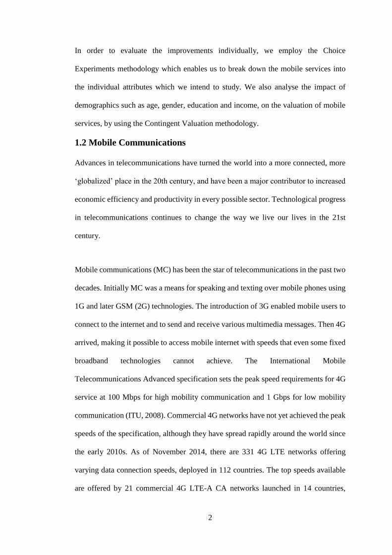
1.2 Mobile Communications
Advances in telecommunications have turned the world into a more connected, more
‘globalized’ place in the 20th century, and have been a major contributor to increased
economic efficiency and productivity in every possible sector. Technological progress
in telecommunications continues to change the way we live our lives in the 21st
century.
Mobile communications (MC) has been the star of telecommunications in the past two
decades. Initially MC was a means for speaking and texting over mobile phones using
1G and later GSM (2G) technologies. The introduction of 3G enabled mobile users to
connect to the internet and to send and receive various multimedia messages. Then 4G
arrived, making it possible to access mobile internet with speeds that even some fixed
broadband technologies cannot achieve. The International Mobile
Telecommunications Advanced specification sets the peak speed requirements for 4G
service at 100 Mbps for high mobility communication and 1 Gbps for low mobility
communication (ITU, 2008). Commercial 4G networks have not yet achieved the peak
speeds of the specification, although they have spread rapidly around the world since
the early 2010s. As of November 2014, there are 331 4G LTE networks offering
varying data connection speeds, deployed in 112 countries. The top speeds available
are offered by 21 commercial 4G LTE-A CA networks launched in 14 countries,

3
subscribers of which enjoy downlink data speeds ranging from 225 Mbps to 300 Mbps
(Ericsson, 2014).
Numerous prior studies have focused on the MC sector. However, rapidly changing
technologies continue to open up new territories for academic and empirical research.
Previous literature has touched on MC licensing and auctions (Klemperer, 2002;
Fuentelsaz et al., 2008), mobile tariff discrimination (Haucap and Heimeshoff, 2011),
mobile roaming (Fabrizi and Wertlen, 2008; Stühmeier, 2012), MC adoption (Rice and
Katz, 2003; Pagani, 2004; Bouwman et al., 2007), and consumer preferences for MC
services (Kim, 2005; Shin et al., 2011; Kwak and Yoo, 2012; Klein and Jakopin, 2014).
In this dissertation, we present a brand-new study on the last of the subject areas in
this list.
1.3 MC Improvements
Our study is focused towards estimating consumer preferences and their determinants
for a selection of ‘current and crucial’ improvements in MC services. The attributes
we evaluate are: increased mobile internet speed, unlimited mobile internet use,
improved quality of communications service, and unrestrained use abroad. These
service upgrades are missing in most mobile markets around the world, and each one
is of interest for a reason.
Although 4G is deployed in many countries, there are still many regions that are not
covered, and many more that are covered but lagging behind in terms of 4G
technology. Consumers of mobile services in these regions have yet to fully benefit
from the features of 4G, namely increased mobile internet speed and improved quality.
Therefore, understanding the value of introducing these features continues to be of

4
interest. Unlimited mobile internet use is interesting because most mobile broadband
services on offer have data caps, whereas fixed broadband services generally provide
unlimited use. Mobile broadband could become a competitor of fixed broadband if
offered with unlimited use, so we aim to quantify the value that consumers associate
with this attribute. Finally, unrestrained use abroad is of interest because people are
travelling more than ever, and operators are charging excessively for roaming mobile
services. The reason for high roaming prices is the lack of competition at the level of
inter-operator tariff negotiation (Salsas and Koboldt, 2004; Sutherland, 2012). The EU
has taken steps to regulate its roaming market (Shortall, 2010; Infante and Vallejo,
2012), and recently independent countries have started to make bilateral agreements
for coordinated action on roaming services (Singapore and Malaysia in 2011 (The
Independent, 2011), Australia and New Zealand in 2013 (MBIE, 2013)). We might
expect to see more countries follow suit in the near future, if the value for the
consumers is depicted more clearly.
Our aim in this study is to evaluate consumers’ willingness to pay (WTP) for the
abovementioned attributes, as a measure of their value. We conduct 320 face-to-face
interviews with people from all regions of North Cyprus, asking respondents to choose
between their existing mobile service and two other hypothetical alternatives with
varying attribute levels. We estimate consumers’ marginal WTP (MWTP) for each
attribute by analysing how they trade off between price and other attributes when
making their choices. We also examine the sensitivity of the WTP for 4G with regard
to demographic characteristics, such as age, gender, education and income levels.
North Cyprus is a developing economy in the Eastern Mediterranean with a population
slightly below 300,000. Mobile use is spread widely throughout the country and the

5
currently available mobile technology is 3G. The results of this study are useful for the
government of North Cyprus in designing a possible auction or tender for 4G licensing,
and for mobile network operators in analysing the costs and benefits of future 4G
investment. Similarly, these results should be of interest for all developing countries,
and especially for Turkey, the 20th largest mobile market in the world in terms of
number of subscribers in 2013 (ITU, 2015). Like North Cyprus, Turkey has not yet
introduced 4G (as of the date of the study), and the same operators dominate both the
Turkish market and the market in North Cyprus (Turkcell and Vodafone).
To the best of our knowledge, this is the first study in literature estimating the value
of various levels of 4G data rates, including the top rate possible as of today. Our
model allows us to estimate non-linear effects of data rates on consumer utility. We
specifically test for a modest improvement to 30 Mbps, and for a more advanced
upgrade to 300 Mbps. We aim to quantify the MWTP for each speed level separately,
so we can evaluate whether there is sufficient demand for the most advanced
technology, or whether the consumers are indifferent between the two levels. This
study is also unique because it is the first attempt in MC literature to estimate the value
of free roaming (use as in homeland) for the consumers. We expect that the results will
draw attention to bilateral roaming regulation, which very few states (EU, Singapore-
Malaysia, Australia-New Zealand) have introduced until today.
1.4 Dissertation Outline
This dissertation is organised as described in the following. Literature review is
presented in Chapter 2. The chapter covers the methodologies to evaluate the
willingness to pay for a service or commodity. In particular, we lay the theoretical
framework for the Averting Expenditure, Choice Experiment, and Contingent

6
Valuation methodologies. Chapter 3 contains the steps followed for the design of the
Choice Experiment that we use in this dissertation to study the demand for various
improvements in mobile services. Chapter 4 depicts the contents of the questionnaire
and discusses the administration of the survey. The chapter also presents the survey
statistics. Chapter 5 revisits the CE model, and displays the results of the CE analysis.
Chapter 6 presents the CVM findings, and also contains a sensitivity analysis which
estimates the relation of WTP with demographic characteristics. Last, Chapter 7
discusses the results of the study and concludes.

7
Chapter 2
2 LITERATURE REVIEW
2.1 Introduction
There are two main approaches to estimating Willingness-To-Pay values for a service
improvement: the revealed preference approach and the stated preference approach.
The revealed preference approach estimates WTP by observing people’s actions which
reveal their preferences. The Averting Expenditure method is the method commonly
used in this approach. This methodology measures WTP by observing the actual
expenditures made by consumers in order to cope with the shortage of the service in
question. By observing this “averting” expenditure of consumers, their revealed WTP
can be estimated.
The stated preference approach, on the other hand, estimates WTP by asking people
to state their preferences. We employ two methods of measuring stated WTP:
Contingent Valuation method and Choice Experiments.
The Contingent Valuation method of measuring stated WTP involves surveying
consumers and asking them to state their willingness to pay for the service
improvement directly. This method of valuing WTP was first proposed by Siegfried
von Ciriacy-Wantrup (1947) as a method of quantifying the benefits of a good or a
service which is not available in the market. As part of a contingent valuation study,

8
we held a survey in North Cyprus in order to understand the importance of 4G service
for the consumers and to elicit their valuation of high-speed mobile service.
The Choice Experiments (CE) method is similar to the Contingent Valuation method
in that it involves surveying people to elicit WTP information. However, contrary to
CVM which produces one estimate for the total value of the service upgrade, CE
method can be used to calculate marginal WTP values for several attributes of the
service improvement. By this way, CE method enables us to fulfil the main purpose of
a CBA analysis, which is to assess and compare various alternatives of a project.
2.2 Willingness-To-Pay or Willingness-To-Accept?
In previous sections, we stated that we take on estimating Willingness-To-Pay values
in order to quantify the magnitude of demand for MC improvements. However, why
should we use Willingness-To-Pay, and not Willingness-To-Accept? What is the
difference between WTP and WTA, in the first place? We first touch the literature on
WTP and WTA.
In order to put things into context, let us focus on a single quality improvement in the
mobile service: the mobile internet speed, and let us denote the level of the speed
available to a consumer with 𝑆. When the speed rises from a level of 𝑆0 to 𝑆1, the
consumer’s utility increases from 𝑈0 to 𝑈1. The welfare impact of the quality
improvement in the mobile internet service refers to the economic value of the
improved quality for the consumer. This value can be measured in two ways: the
compensating variation and the equivalent variation (Silberberg and Suen, 2001).
Compensating variation (CV) is the amount which should be removed from income at
the new speed level 𝑆1, in order to bring the consumer back to the initial utility level

9
𝑈0. In other words, CV measures the consumer’s maximum willingness to pay (WTP)
for the quality improvement. The indirect utility representation of compensating
variation would be as follows:
𝑉(𝑝0, 𝑆0, 𝑌) = 𝑉(𝑝0, 𝑆1, 𝑌 − 𝐶𝑉)
where V is the indirect utility function, 𝑝0 is the vector of prices and 𝑌 is the
consumer’s income. Using the expenditure function 𝑒(. ), we can rearrange this
equation to write CV explicitly:
𝐶𝑉 = 𝑒(𝑝0, 𝑆0, 𝑈0)– 𝑒(𝑝0, 𝑆1, 𝑈0)
Equivalent variation (EV) is the amount of income which the consumer should be
granted at the initial speed level 𝑆0 in order to move the consumer from the utility
level 𝑈0 to 𝑈1. In other words, EV refers to the minimum willingness of the consumer
to accept (WTA) not to receive the speed upgrade. Again, using indirect utility
function, we represent this as:
𝑉(𝑝0, 𝑆0, 𝑌 + 𝐸𝑉) = 𝑉(𝑝0, 𝑆1, 𝑌)
Rearranging to express EV explicitly using the expenditure function:
𝐸𝑉 = 𝑒(𝑝0, 𝑆0, 𝑈1)– 𝑒(𝑝0, 𝑆1, 𝑈1)
WTP and WTA values for a quality improvement are usually not equal to each other
(Randall & Stoll, 1980; Horowitz & McConnell, 2002; Biel, Johansson-Stenman &
Nilsson, 2006). WTA figures are greater than WTP figures, due to reasons such as
income and substitution effects, price flexibility of income, and the tendency for loss
aversion. Because of the sizable differences in the absolute values of WTP and WTA,
we need to make a choice in order to assign a value for the welfare impact of the
service improvement. Practitioners of the CBA like Mitchell and Carson (1989) or the

10
members of the NOAA panel (1993) recommend to always use WTP for practical
purposes, since WTP is the conservative choice and should be preferred to be on the
safe side.
2.3 Revealed Preference Approach
Revealed Preference techniques for estimating WTP for a service quality improvement
include direct demand estimation, hedonic price analysis, travel cost analysis, cost of
illness analysis, and averting expenditure analysis. Direct demand technique
necessitates adequate time-series sales data, the prices of the service sold, the level of
the service quality, and other economic data such as income data, other relevant prices
in the market, and demographic data. Due to the unavailability of this kind of data,
especially in developing countries, this technique is rarely used. On the other hand,
hedonic price, travel cost analysis, and cost of illness analysis are specifically used for
the assessment of environmental policies. Averting expenditure analysis is the
approach most widely used.
2.3.1 Averting Expenditure
The Averting Expenditure method makes use of the theory of production function
(Becker, 1965; Bockstael & McConnell 1999). According to this theory, consumer’s
utility is a function of commodities and services which the consumer produces herself,
and the characteristics of the consumer. Rearranging the production theory for our
purposes, we can state consumer’s utility to be a function of MC dependent services,
commodities/services other than the MC dependent services, and the consumer’s
characteristics.
𝑈 = 𝑈(𝑍(𝑁, 𝐴, 𝑆), 𝑋, 𝜏)
where 𝑍 is the production function of MC dependent services (talking, messaging,
surfing the net, gaming, etc.), 𝑁 is the amount of the mobile service used, 𝐴 is the

11
amount of averting actions, 𝑆 is the speed of current mobile service available to the
consumer, 𝑋 is the amount of other commodities and services consumed, and 𝜏
represents the characteristics of the consumer. Given the speed of current mobile
service available to the consumer (if the consumer decides to subscribe), the consumer
picks the minimum amount to spend, as averting expenditure, in order to produce the
optimum level of MC dependent services that will maximise her utility subject to her
budget constraint. Put differently, the consumer has an optimal level of MC dependent
services, which depends on her income, prices, consumption of other goods,
characteristics, among other things. Therefore, if the real speed 𝑆 of current mobile
service available to the consumer is not sufficient to produce the consumer’s optimal
level of MC dependent services, the consumer partakes in averting behaviour that will
raise these services to the desired level.
Bartik (1988) shows the lower and upper bounds of the welfare impact of a reduction
in pollution can be calculated using averting expenditure data. Using the approach of
Bartik (1988), we lay the theoretical framework for using AE method to calculate the
lower bound of the welfare impact of a mobile service upgrade.
The cost function of producing MC dependent services, 𝐶𝑍(. ) is defined as:
𝐶𝑍 = 𝐶𝑍(𝑍(𝑁, 𝐴, 𝑆), 𝑝𝑁, 𝑝𝐴, 𝑆)
where 𝑝𝑁 is the price of current mobile service, and 𝑝𝐴 is the price vector of the
averting actions. Let 𝑍∗ be the optimal level of MC dependent services for a consumer
that faces current mobile internet speed level 𝑆0. If the mobile speed rises from 𝑆0 to
𝑆1, the cost to produce this optimal level 𝑍∗ decreases by:
𝐶𝑍(𝑍∗, 𝑝𝑁 , 𝑝𝐴, 𝑆0)– 𝐶𝑍(𝑍∗, 𝑝𝑁 , 𝑝𝐴, 𝑆1)

12
Let us denote the restricted expenditure function 𝑒(. ) which gives the minimum
expenditure needed to provide utility 𝑈 when mobile internet speed available is 𝑆, the
prices are 𝑝, and the consumer’s optimal level of MC dependent services is restricted
to 𝑍, as follows:
𝑒(𝑝, 𝑆, 𝑈; 𝑍)
We can argue that, when mobile internet speed rises from 𝑆0 to 𝑆1, the decrease in
expenditures needed to achieve the optimal level of services 𝑍∗, is equal to the drop in
the cost of producing 𝑍∗:
𝑒(𝑝, 𝑆0, 𝑈0) – 𝑒(𝑝, 𝑆1, 𝑈0; 𝑍∗) = 𝐶𝑍(𝑍∗, 𝑝𝑁, 𝑝𝐴, 𝑆0)– 𝐶𝑍(𝑍∗, 𝑝𝑁, 𝑝𝐴, 𝑆1)
Rearranging the equation above:
𝑒(𝑝, 𝑆0, 𝑈0) = 𝐶𝑍(𝑍∗, 𝑝𝑁 , 𝑝𝐴, 𝑆0)– 𝐶𝑍(𝑍∗, 𝑝𝑁 , 𝑝𝐴, 𝑆1) + 𝑒(𝑝, 𝑆1, 𝑈0; 𝑍∗)
We can substitute in the expression for the CV of an upgrade in the speed of mobile
internet, which we derived in section 2.2:
𝐶𝑉 = 𝑒(𝑝, 𝑆0, 𝑈0)– 𝑒(𝑝, 𝑆1, 𝑈0)
and we arrive at the following equation:
𝐶𝑉 = 𝐶𝑍(𝑍∗, 𝑝𝑁 , 𝑝𝐴, 𝑆0)– 𝐶𝑍(𝑍∗, 𝑝𝑁 , 𝑝𝐴, 𝑆1) + 𝑒(𝑝, 𝑆1, 𝑈0; 𝑍∗) −
𝑒(𝑝, 𝑆1, 𝑈0)
Notice that, on the right hand side of the equation, the third term is larger than the last
term. With the mobile speed improved to 𝑆1, the required expenditure to achieve utility
𝑈0 is larger if the level of internet dependent services is restricted to 𝑍∗. This is
because, if the level of 𝑍 is not restricted, utility 𝑈0 can be achieved with fewer
expenditure by allowing people to increase their level of 𝑍. Therefore, the CV of
service quality improvement is equal to the drop in the cost of producing 𝑍∗ and a

13
positive term. Hence, we may conclude the cost savings achieved by improving mobile
speed S when holding 𝑍 constant is a minimum estimate of the welfare impact of the
mobile internet speed change.
The consumer utility maximization problem is:
𝑀𝑎𝑥𝑋,𝑁,𝐴 𝑈(𝑍(𝑁, 𝐴, 𝑆), 𝑋, 𝜏) 𝑠𝑢𝑏𝑗𝑒𝑐𝑡 𝑡𝑜 𝐶𝑍(𝑍, 𝑝𝑁, 𝑝𝐴, 𝑆) + 𝑝𝑋𝑋 ≤ 𝑌, 𝑎𝑛𝑑
𝐶𝑍(𝑍, 𝑝𝑁 , 𝑝𝐴, 𝑆) = Min𝐴,𝑁 (𝑝𝐴𝐴 + 𝑝𝑁𝑁) 𝑠𝑢𝑏𝑗𝑒𝑐𝑡 𝑡𝑜 𝑍 = 𝑍(𝑁, 𝐴, 𝑆)
The solution to this utility maximization problem is given by the indirect utility
function,
𝑉 = 𝑉(𝑝𝑋, 𝑝𝑁, 𝑝𝐴, 𝑌, 𝑆, 𝜏)
Using Roy’s theorem, we can obtain the optimum level of averting actions:
𝐴 =𝜕CZ
𝜕𝑝𝐴= −
𝜕𝑉 𝜕𝑝𝐴⁄
𝜕𝑉 𝜕𝑌⁄= 𝐴(𝑝𝑋 , 𝑝𝑁 , 𝑝𝐴, 𝑆, 𝑍(𝑝𝑁, 𝑝𝐴, 𝑝𝑋 , 𝑌, 𝑆, 𝜏))
2.4 Stated Preference Approach
Stated Preference Approach for estimating Willingness-To-Pay for a service quality
improvement involves extracting the value people associate with the quality
improvement via surveys. Two common techniques, which we will employ for mobile
service improvement in North Cyprus as well, are Contingent Valuation Methodology
and Choice Experiments Methodology.
2.4.1 Contingent Valuation Methodology
In the CVM method, a survey is held and respondents are asked to state their WTP
directly. This method is used to evaluate a variety of goods and services. Several
examples include: Amirnejad, Hamid, et al. (2006) estimating the existence value of
north forests of Iran; Lee, Choong-Ki, and Sang-Yoel Han (2002) estimating the use
and preservation values of national parks’ tourism resources in South Korea; and
14
Montes de Oca and Bateman (2006) estimating WTP for water services in Mexico
City.
Although CVM is widely used for estimating WTP, this methodology has its critics.
Venkatachalam (2004) reviews the possible pitfalls of CVM, which it has often
received criticism for:
Embedding effect: Variation in estimated WTP for a commodity or service depending
on whether it is evaluated on its own or as part of a bundle.
Sequencing effect: Variation in estimated WTP depending on the order in which it is
asked in the survey (in studies estimating WTP for more than one good).
Information effect: Variation in estimated WTP due to the level of information
provided.
Elicitation effect: Variation in estimated WTP due to the elicitation technique used
(bidding game, payment card, open-ended elicitation technique, single-bounded
dichotomous choice approach, double-bounded dichotomous choice approach).
Hypothetical bias: Divergence between true WTP and stated WTP
Strategic bias: Occurs if the survey takers hide their true WTP for strategic reasons.
Payment vehicle bias: Variation in estimated WTP due to the type of payment vehicle
(income tax, entry fee, utility bill, etc.).

15
Despite the criticisms, there are ways suggested in the literature to keep potential
biases to a minimum, and CVM continues to be an effective tool to elicit WTP
information (Whittington 1998; List, 2001; Arrow et al., 2001).
2.4.1.1 Theory behind the CVM Method
There are three different approaches within the CVM methodology, as follows:
Random utility approach: This approach starts from the utility function, and makes
assumptions about the functional form of the utility function and the probability
distribution of the error term in the utility function.
Parametric modelling of the WTP: This starts from the WTP function, and makes
assumptions about the functional form of the WTP function and the error term of the
WTP function.
Non-parametric modelling of the WTP: Starts from the WTP function, and makes some
assumption about the shape of the WTP function (as few assumptions as possible) and
no assumption about an error term (deterministic model).
2.4.1.2 Random Utility Approach in CVM
The random utility approach, as the name suggests, makes use of the random utility
theory. In order to demonstrate, we follow Hanemann (1984) and we adopt his
approach to our mobile services case.
Let us assume, as part of the CVM study, an individual 𝑞 is told the speed of the mobile
service will increase from 𝑆0 to 𝑆1, and the cost of this improvement will be 𝐵𝑞. Then
the individual is queried as to whether she is willing to pay the cost 𝐵𝑞 for the

16
improvement in the mobile internet speed. The individual’s response, represented by
variable 𝑖, is either a “yes” (in which case, 𝑖 = 1), or a “no” (𝑖 = 0).
The utility of the individual 𝑞 from alternative 𝑖 is made of an observable component
and a random component:
𝑈𝑖𝑞 = 𝑉𝑖𝑞 + 𝜀𝑖𝑞
The component 𝑉𝑖𝑞 is observable to the researcher, and the random component 𝜀𝑖𝑞 is
not. 𝑉𝑖𝑞 is given by:
𝑉𝑖𝑞 = 𝑉𝑖𝑞(𝑝𝑋, 𝑝𝑁 , 𝑝𝐴, 𝑆, 𝑌; 𝜏𝑞)
where 𝑝𝑁 is the price of mobile service, 𝑝𝐴 is the price vector for the averting actions,
𝑝𝑋 is the price vector of all other goods/services, 𝑆 is the speed of mobile internet, 𝑌
is income, and 𝜏𝑞 is a vector of the individual’s characteristics.
When asked whether she is willing to pay the amount 𝐵𝑞, the individual will accept
the offer if her utility after paying the amount 𝐵𝑞 to reach speed 𝑆1 is greater than, or
at least equal to, her initial utility at speed 𝑆0 and not having paid the amount 𝐵𝑞. This
is to say, she will accept the offer if:
𝑉1𝑞(𝑝𝑋 , 𝑝𝑁 , 𝑝𝐴, 𝑆1, 𝑌 − 𝐵𝑞; 𝜏𝑞) + 𝜀1𝑞 ≥ 𝑉0𝑞(𝑝𝑋, 𝑝𝑁 , 𝑝𝐴, 𝑆0, 𝑌; 𝜏𝑞) + 𝜀0𝑞
Rearranging;
𝑉1𝑞(𝑝𝑋 , 𝑝𝑁 , 𝑝𝐴, 𝑆1, 𝑌 − 𝐵𝑞; 𝜏𝑞) − 𝑉0𝑞(𝑝𝑋, 𝑝𝑁, 𝑝𝐴, 𝑆0, 𝑌; 𝜏𝑞) ≥ 𝜀0𝑞 − 𝜀1𝑞
The right hand side is not observable to the researcher, and therefore it is a random
variable. Hence, the response of the individual is also a random variable. We can
express its probability distribution as follows:

17
𝑃1𝑞 = 𝑃( 𝑉1𝑞(𝑝𝑋, 𝑝𝑁 , 𝑝𝐴, 𝑆1, 𝑌 − 𝐵𝑞; 𝜏𝑞) − 𝑉0𝑞(𝑝𝑋 , 𝑝𝑁 , 𝑝𝐴, 𝑆0, 𝑌; 𝜏𝑞) ≥ 𝜀0𝑞 −
𝜀1𝑞 )
𝑃1𝑞 is the probability the individiual is willing to pay the cost. Then, the probability
that the individual is not willing to pay the cost, 𝑃0𝑞, is given by:
𝑃0𝑞 = 1 − 𝑃1𝑞
Assuming the random errors are independent and identically distributed with a mean
of 0, we can define 𝜂 = 𝜀0𝑞 − 𝜀1𝑞, and let 𝐹𝜂 be the cumulative distribution function
of 𝜂. Then, 𝑃1𝑞 and 𝑃0𝑞 are shortly:
𝑃1𝑞 = 𝐹𝜂(𝛥𝑉), 𝑃0𝑞 = 1 − 𝐹𝜂(𝛥𝑉), 𝑤ℎ𝑒𝑟𝑒 𝛥𝑉 = 𝑉1𝑞 − 𝑉0𝑞.
Now, let 𝐼𝑞 be an indicator variable for the individual 𝑞. Then, the log-likelihood
function for all 𝑁 individuals in the survey is:
log 𝐿 = ∑ 𝐼𝑞 ln 𝐹𝜂(𝛥𝑉) + (1 − 𝐼𝑞) ln (1 − 𝐹𝜂(𝛥𝑉))𝑁𝑞=1
At this point, in order to carry out a Maximum Likelihood estimation and find the
parameters that maximize the likelihood, we need to make assumptions about the
functional form of the utility function and the distribution of the error term. The
simplest assumptions would be a linear utility function and a normal distribution for
the error terms (Probit). The utility function would be given as:
𝑈𝑖𝑞 = 𝑉𝑖𝑞 + 𝜀𝑖𝑞
𝑈𝑖𝑞 = 𝛼𝑖 + 𝜇𝑌 + 𝜀𝑖𝑞
The utility levels for the responses “Yes” and “No” are:
𝑈0𝑞 = 𝛼0 + 𝜇𝑌 + 𝜀0𝑞

18
𝑈1𝑞 = 𝛼1 + 𝜇(𝑌 − 𝐵𝑞) + 𝜀1𝑞
𝛥𝑉 is given by:
𝛥𝑉 = 𝑉1𝑞 − 𝑉0𝑞 = 𝛼1 − 𝛼0 − 𝜇𝐵𝑞 = 𝛼 − 𝜇𝐵𝑞 , 𝑤ℎ𝑒𝑟𝑒 𝛼 = 𝛼1 − 𝛼0.
From our previous result we have:
𝑃1𝑞 = 𝑃(𝛥𝑉 ≥ 𝜀0𝑞 − 𝜀1𝑞 ) = 𝑃(𝛼 − 𝜇𝐵𝑞 ≥ 𝜂)
Since we assumed error term to be normally distributed, 𝜂 is also I.I.D. (independent
identically distributed) with normal distribution:
𝜂 ~ 𝑁(0, 𝜎2)
In order to convert this into a standard normal distribution, we define 𝜃:
𝜃 = 𝜂 𝜎⁄ , 𝜃 ~ 𝑁(0,1)
Then 𝑃1𝑞 is:
𝑃1𝑞 = 𝑃(𝜂 ≤ 𝛼 − 𝜇𝐵𝑞) = 𝑃 (𝜂
𝜎≤
𝛼
𝜎−
𝜇
𝜎𝐵𝑞) = 𝑃 (𝜃 ≤
𝛼
𝜎−
𝜇
𝜎𝐵𝑞) = 𝛷 (
𝛼
𝜎−
𝜇
𝜎𝐵𝑞)
where 𝛷(. ) is the cumulative distribution function of standard normal distribution. We
can therefore estimate two parameters 𝛼
𝜎 and
𝜇
𝜎.
Remember we are interested in WTP. We can use the estimations of these parameters
in order to calculate the mean and the median of WTP. The mean (or expected value)
of WTP is the most natural measure of WTP. The median is of interest because this is
the level of WTP at which there is 50:50 chance that the response will be “Yes”.

19
Here is how to solve for mean and median WTP. WTP is the maximum amount of
money an individual is willing to pay for the service improvement, so she is indifferent
between having the service improvement and not having the service improvement:
𝛼0 + 𝜇𝑌 + 𝜀0𝑞 = 𝛼1 + 𝜇(𝑌 − 𝑊𝑇𝑃𝑞) + 𝜀1𝑞
Solving for WTP gives:
𝑊𝑇𝑃𝑞 =𝛼+𝜂
𝜇
Then the mean (expected value) is given as:
𝐸[𝑊𝑇𝑃𝑞] = 𝐸 [𝛼+𝜂
𝜇] =
𝛼
𝜇+
𝐸[𝜂]
𝜇=
𝛼
𝜇
The median, represented by 𝑊𝑇𝑃∗, is the willingness to pay amount at which there is
50 per cent chance the response will be “Yes”:
𝑃1𝑞 = 𝐹𝜂(𝛥𝑉(𝑊𝑇𝑃𝑞∗)) = 0.5
Since we assumed error term to be normally distributed, the above occurs when:
𝐹𝜂(0) = 0.5
and hence:
𝛥𝑉(𝑊𝑇𝑃𝑞∗) = 𝛼 − 𝜇𝑊𝑇𝑃𝑞
∗ = 0
Solving for 𝑊𝑇𝑃𝑞∗, we get the median of WTP to be the same as mean WTP:
𝑊𝑇𝑃𝑞∗ =
𝛼
𝜇
2.4.1.3 Parametric Modelling of the WTP in CVM
Alternatively, we can start with specifying a functional form of WTP and a
distributional assumption about the error term in the WTP function. Let us again make
the simplest assumptions; a linear WTP function and a normal distribution for the error
term. The linear WTP function is given by:
𝑊𝑇𝑃𝑞 = 𝛽𝑋𝑞 + 𝜀𝑞
20
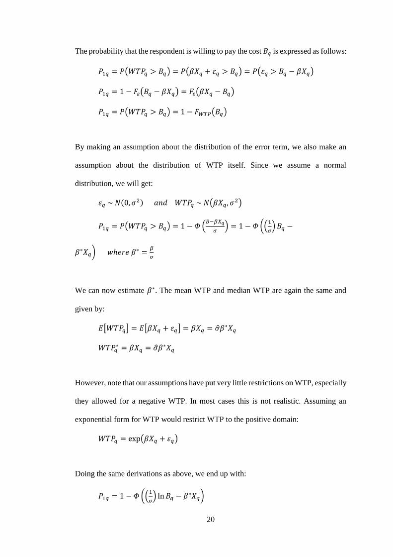
The probability that the respondent is willing to pay the cost 𝐵𝑞 is expressed as follows:
𝑃1𝑞 = 𝑃(𝑊𝑇𝑃𝑞 > 𝐵𝑞) = 𝑃(𝛽𝑋𝑞 + 𝜀𝑞 > 𝐵𝑞) = 𝑃(𝜀𝑞 > 𝐵𝑞 − 𝛽𝑋𝑞)
𝑃1𝑞 = 1 − 𝐹𝜀(𝐵𝑞 − 𝛽𝑋𝑞) = 𝐹𝜀(𝛽𝑋𝑞 − 𝐵𝑞)
𝑃1𝑞 = 𝑃(𝑊𝑇𝑃𝑞 > 𝐵𝑞) = 1 − 𝐹𝑊𝑇𝑃(𝐵𝑞)
By making an assumption about the distribution of the error term, we also make an
assumption about the distribution of WTP itself. Since we assume a normal
distribution, we will get:
𝜀𝑞 ~ 𝑁(0, 𝜎2) 𝑎𝑛𝑑 𝑊𝑇𝑃𝑞 ~ 𝑁(𝛽𝑋𝑞 , 𝜎2)
𝑃1𝑞 = 𝑃(𝑊𝑇𝑃𝑞 > 𝐵𝑞) = 1 − 𝛷 (𝐵−𝛽𝑋𝑞
𝜎) = 1 − 𝛷 ((
1
𝜎) 𝐵𝑞 −
𝛽∗𝑋𝑞) 𝑤ℎ𝑒𝑟𝑒 𝛽∗ =𝛽
𝜎
We can now estimate 𝛽∗. The mean WTP and median WTP are again the same and
given by:
𝐸[𝑊𝑇𝑃𝑞] = 𝐸[𝛽𝑋𝑞 + 𝜀𝑞] = 𝛽𝑋𝑞 = �̂�𝛽∗𝑋𝑞
𝑊𝑇𝑃𝑞∗ = 𝛽𝑋𝑞 = �̂�𝛽∗𝑋𝑞
However, note that our assumptions have put very little restrictions on WTP, especially
they allowed for a negative WTP. In most cases this is not realistic. Assuming an
exponential form for WTP would restrict WTP to the positive domain:
𝑊𝑇𝑃𝑞 = exp(𝛽𝑋𝑞 + 𝜀𝑞)
Doing the same derivations as above, we end up with:
𝑃1𝑞 = 1 − 𝛷 ((1
𝜎) ln 𝐵𝑞 − 𝛽∗𝑋𝑞)

21
𝐸[𝑊𝑇𝑃𝑞] = exp( �̂�𝛽∗𝑋𝑞) exp (1
2�̂�2)
2.4.1.4 Non-Parametric Modelling of the WTP in CVM
The parametric approaches to estimate WTP described above require assumptions
about distributions, and therefore they risk resulting in erratic results if the assumptions
do not hold. As an alternative, several studies (Turnbull, 1976; Kriström, 1990)
suggested a non-parametric approach to estimating WTP using a CVM survey.
In this non-parametric approach, respondents of the CVM survey are asked to answer
“Yes” or “No” to whether they are willing to pay a cost of 𝐵. There are 𝑚 different
costs presented to 𝑚 different samples with each sub-sample 𝑖 having 𝑛𝑖 individuals.
If we let 𝑘𝑖 represent the number of individuals saying “Yes” to 𝐵𝑖 in each sub-sample
𝑖, then the proportion of “Yes” answers in this sub-sample is given by 𝑝𝑖 =𝑘𝑖
𝑛𝑖 .
Calculating 𝑝𝑖 for all sub-samples 𝑖 = 1 to 𝑚, we end up with a sequence
𝑝1, 𝑝2, 𝑝3, … , 𝑝𝑚−1, 𝑝𝑚 which can be interpolated with an appropriate rule to arrive at
a function for the probability of Yes answers in terms of the bid amount 𝐵. Mean
willingness to pay can simply be estimated as the area under this curve.
“Kaplan-Meier-Turnbull” and “Spearman-Karber” estimations are two commonly
used non-parametric estimates of mean WTP. The KMT and SK estimators are given
by:
𝐸𝐾𝑀𝑇[𝑊𝑇𝑃] = ∑ 𝐵𝑖(𝑝𝑖 − 𝑝𝑖+1)𝑚𝑖=1
𝐸𝑆𝐾[𝑊𝑇𝑃] = ∑ ((𝐵𝑖+𝐵𝑖+1)(𝑝𝑖−𝑝𝑖+1)
2)𝑚
𝑖=1
2.4.2 Choice Experiments Methodology
Origins of the CE methodology date back to Louis L. Thurstone’s 1927 paper in
Psychological Review on paired (comparison) choice experiments. Many authors have

22
contributed to the literature on choice analysis, and the final methodology of Choice
Experiments draws upon Lancaster’s economic theory of value (Lancaster, 1966) and
random utility theory (McFadden, 1973; Hanemann, 1984). CE is now commonly used
in various fields of economics and marketing to make choice-based valuations of
goods, services and their attributes.
What sets CE apart from CVM is that CE allows researchers to study not only the
value of a commodity itself, but also the values of various attributes of this commodity.
These attributes are the main sources influencing people’s decisions, and hence, the
value people associate to each attribute is precious information. In order to extract this
information, the CE practitioner designs choice sets which contain different levels of
the attributes, and asks people in a survey to make choices between these sets. By this
way, the CE practitioner is able to analyse the marginal effect of each individual
attribute.
In the context of this dissertation, Choice Experiments methodology enables us to
decompose the improvement in mobile service into various attributes, such as the
speed of the mobile internet service, the quality, the amount of use offered (i.e. whether
the service is limited or unlimited), and more. While CVM produces a single value of
WTP for the service improvement, CE estimates a separate marginal WTP for each
individual attribute studied. Therefore, with Choice Experiments, we are able to assess
and compare various alternatives for the MC improvement project, and produce more
meaningful policy implications.
Choice Experiments are widely used in estimating the welfare impact of public
policies. Several examples include valuing forest landscapes in UK (Hanley, Wright

23
and Adamowicz, 1998), wetlands in South Sweden (Carlsson, Frykblom and
Liljenstolpe, 2003) and health programs in US, UK, Australia and Canada (Ryan and
Gerard, 2003). Choice Experiments have also been used to analyse the demand for
mobile services which is the focus of this dissertation. Kim (2005) estimated consumer
preferences for IMT-2000 (3G) services in South Korea, Shin et al. (2011) carried out
a similar conjoint analysis for mobile service consumption in Uzbekistan, and the first
CE study evaluating consumers’ preferences for 4G technology was by Kwak and Yoo
(2012).
2.4.2.1 Theory behind the CE Methodology
As stated before, CE methodology makes use of the random utility theory. An
individual, when faced with an alternative 𝑖, derives a utility from this alternative as
follows:
𝑈𝑖 = 𝑉𝑖 + 𝜀𝑖
The component 𝑉𝑖 is observable to the researcher, and the random component 𝜀𝑖 is
not. The observed component 𝑉𝑖 is where the set of attributes which are observable
and measurable reside. The simplest assumption for 𝑉𝑖 would be that it is a linear
function of the attributes, each of which is weighted by a unique weight to account for
that attribute’s marginal utility input. Using 𝑓 as a generalized notation for functional
form but noting that the functional form can be different for each attribute, we can
write 𝑉𝑖 as:
𝑉𝑖 = 𝛽0𝑖 + 𝛽1𝑖𝑓(𝑋1𝑖) + 𝛽2𝑖𝑓(𝑋2𝑖) + 𝛽3𝑖𝑓(𝑋3𝑖) + ⋯ + 𝛽𝐾𝑖𝑓(𝑋𝐾𝑖)
where 𝑋𝑘𝑖 represent the 𝑘 = 1 to 𝐾 attributes of alternative 𝑖, 𝛽𝑘𝑖 represent the weights
of these attributes, and 𝛽0𝑖 is a parameter which is not associated with any observed
attribute but represents the role of all unobserved sources of utility.

24
If we treat each attribute to be linear so that 𝑓(𝑋) = 𝑋, and if we assume the random
component of utility 𝜀𝑖 to be inclusive of all sources of variance from unobserved
components of 𝛽 and 𝑋, and also if we assume 𝜀𝑖 to be IID (independently and
identically distributed), we end up with the Multinomial Logit (MNL) model:
𝑈 = 𝛽1𝑋1 + 𝛽2𝑋2 + 𝛽3𝑋3 + ⋯ + 𝛽𝐾𝑋𝐾 + 𝜀
The assumption that all sources of variance are encapsulated by 𝜀 is a very strong
assumption, and it might not always be realistic. For example, the MNL model
assumes the attributes that are not included in the observed part of the utility expression
are represented by the unobserved component and of identical impact for each
alternative. If the alternatives are mobile service technologies (i.e. GSM, 3G, 4G, etc),
and the data rate is missing in the attributes, it would be unrealistic to assume data rate
has the exact same influence on the choice of each alternative (ie. 3G vs. 4G).
Moreover, sometimes an attribute is common to two or more alternatives. If this
attribute is excluded from the observed part of the utility expression, then its inclusion
in the unobserved component will introduce correlation between alternatives, and the
IID assumption will be violated. Therefore, when there is concern that there will be
correlation between alternatives because of an inability to accommodate the sources
of this in the observed part of utility, one should opt for a less restrictive model. For
instance, Nested Logit model and Mixed Logit model have fewer restrictions
compared to MNL. Nested Logit model allows to partition the choice set in a way that
constant variance assumption holds among alternatives in the same partition while
allowing differential variance between partitions. Mixed logit, on the other hand, is
even less restrictive and permits correlation between all pairs of alternatives. There are
various other models as well, that we will not dwell on here.

25
Once the form of the utility expression is identified, we turn to how an individual
makes a choice in a Choice Experiment. Suppose the individual faces 𝑗 = 1 to 𝐽
alternatives. In order to make a choice, the individual will evaluate the utility she will
derive for each alternative and pick the one with the highest utility. Putting this into
notation, the probability that alternative 𝑖 will be chosen is:
𝑃𝑖 = 𝑃 ((𝑈𝑖 ≥ 𝑈𝑗) ∀ 𝑗 ∈ 𝑗 = 1, … , 𝐽; 𝑖 ≠ 𝑗)
Rearranging;
𝑃𝑖 = 𝑃 ((𝑉𝑖 + 𝜀𝑖 ≥ 𝑉𝑗 + 𝜀𝑗) ∀ 𝑗 ∈ 𝑗 = 1, … , 𝐽; 𝑖 ≠ 𝑗)
𝑃𝑖 = 𝑃 (((𝜀𝑗 − 𝜀𝑖) ≤ (𝑉𝑖 − 𝑉𝑗)) ∀ 𝑗 ∈ 𝑗 = 1, … , 𝐽; 𝑖 ≠ 𝑗)
Since the error term is not observable, estimating the model requires picking up a
probability distribution for the error term. A popular distribution in discrete choice
analysis is the extreme value type 1 (EV1) distribution, which has the following form:
𝑃(𝜀𝑗 ≤ 𝜀) = exp(− exp −𝜀)
Equipped with the IID and EV1 assumptions, we can proceed to complete the model.
Louviere, Hensher and Swait (2000, chapter 3) take on the full derivation of the
Multinomial Logit (MNL) model, and end with the following:
𝑃𝑖 =exp 𝑉𝑖
∑ exp 𝑉𝑗𝐽𝑗=1
; 𝑗 = 1, … , 𝑖, … , 𝐽 𝑖 ≠ 𝑗
In words, this states that the probability of an individual choosing alternative 𝑖 out of
𝐽 alternatives is equal to the ratio of the exponential of the observed utility index for
alternative 𝑖 to the sum of the exponentials of the observed utility indices for all 𝐽
alternatives including the 𝑖th alternative.

26
The model can be estimated using maximum likelihood techniques. The parameters to
be estimated are the weights 𝛽 of the attributes in the utility function. Let us say 𝑋
consists of 𝐾 attributes, and one of the attributes is the price attribute 𝑝. Lancsar (2004)
gives the marginal willingness to pay for one attribute 𝑘, and the willingness to pay
for the whole commodity (or service) in question, resulting from all attributes, as
follows:
𝑀𝑊𝑇𝑃𝑘 =
𝑑𝑉
𝑑𝑋𝑘
−𝑑𝑉
𝑑𝑝
=𝛽𝑘
−𝛽𝑝
𝑊𝑇𝑃 = ∑𝛽𝑘
𝛽𝑝(𝛥𝑋𝑘)𝐾
𝑘=1
Similar to CVM, the Choice Experiment methodology has its critics. CE shares the
same potential errors and biases with CVM and any other stated preference method,
such as sequencing effects, elicitation effects, information effects, hypothetical bias
and strategic bias, all of which were mentioned in the previous section. Cummings and
Taylor (1999), List (2001), List et al. (2006), Blumenschein et al. (2008) and Savage
and Waldman (2008) propose methods for minimizing bias in Choice Experiments.
There are also additional issues related with CE that need to be considered before it is
put into practice. CE estimates the marginal value of the attributes and presumes that
the value of the entire commodity/service equals the aggregate of the values of the
attributes. It is questionable that this assumption is valid. In fact, there are studies
which find that the WTP estimates of Choice Experiments are considerably larger than
the estimates of the Contingent Valuation Method (Maynard, 1996). Moreover, CE
methodology is sensitive to design. The choice of alternatives, levels, choice sets in
the design of the experiment can have an impact on the resulting estimates. If the
respondents are given too many alternatives with varying attributes and levels, fatigue

27
may cause them to make unsound choices. Also, there is the possibility of correlation
between the choices made by the same individual due to repeated choice sets
(Louviere, Hensher and Swait, 2000). These are important points of consideration
when designing and using Choice Experiments.
On the other hand, CE method does offer advantages. For one, CE is able to break
down a good or service into its attributes and measure the trade-offs between the
attributes, as mentioned before. If one of these attributes is selected to be price, then
CE can calculate the marginal value of changes in each attribute. For another, the CE
approach determines the levels of attributes of each alternative offered exogenously
and avoids collinearity problems by offering non-existing alternatives. For instance, in
the case of mobile service improvement, speed and quality attributes change
independently in the hypothetical alternatives of a Choice Experiment, whereas they
often vary together almost perfectly in the real market. Hence, the CE approach is able
to extract the impact of speed and quality separately. The last and equally important
advantage of CE is that it is a better simulation of real-world transactions than CVM.
In a CVM study, survey takers are presented with a hypothetical situation, so their
responses and the WTP estimate of the study depend on how accurate the information
in this presentation is. In a CE study, respondents are given alternatives and asked to
make a choice, like they do in reality. The fact that respondents are reminded about
substitutes and complements improves the reliability of the WTP figure estimated by
CE.

28
2.4.3 Review of Selected Consumer Studies on the Value of Broadband Services
(Fixed & Mobile)
Estimating consumer preferences for the attributes of telecommunications services has
been a topic of interest among researchers since the advent of broadband internet in
the 1990s. Earlier studies focused on fixed broadband services, while the focus has
shifted towards mobile services since the 2010s as mobile technologies have caught
up and overtaken fixed technologies. A number of notable stated preference studies
that estimate consumers’ valuations for telecom services and their attributes have been
completed to date.
2.4.3.1 Consumer Studies for Fixed Broadband Services
Madden and Simpson (1997) were among the first to carry out research in this area.
They used data obtained from a national survey of households in Australia in order to
determine the willingness of households to subscribe to a broadband network. The fact
that broadband services were not currently available at that time was a complication
for their study. Out of 1,010 households surveyed, 598 provided usable data. The
authors employed maximum likelihood estimation for a logit model, and found that
the effects of the installation fee and income on the probability of subscription were
statistically significant, whereas the effect of monthly fee was not. Other determinants
for the probability of subscription were the size of the household, the age of the
household head and whether the head was employed in a blue-collar occupation.
Ida and Kuroda (2006) studied the Japanese market for broadband services such as
ADSL, CATV (cable television internet) and FTTH (fibre to the home). They
employed a discrete choice analysis with a nested logit model on a data set of 1,013
observations. They showed that a nested choice structure of narrowband (dial-up,

29
ISDN) versus broadband (ADSL, CATV, FTTH) is the best model fit because of the
sign conditions of price and speed variables, their statistical significance and degrees
of fitness. They also showed that the own-price elasticity of ADSL is inelastic, while
the figures for CATV and FTTH are elastic, concluding that the ADSL market is
independent of other services.
Rosston et al. (2010) produced the most comprehensive CE study on the broadband
internet market in the USA, and for the first time introduced the effects of attributes.
The authors employed discrete choice analysis to estimate the marginal WTP for
improvements in eight internet service characteristics: cost, reliability, speed, laptop
mobility, movie rental, priority, telehealth and videophone. The data was from a
nationwide survey conducted with 6,271 respondents in late 2009 and early 2010. The
results implied that reliability and speed were important characteristics of internet
service. Estimated MWTPs were 20 USD per month for more reliable service, 45 USD
for an improvement in speed from slow to fast, and 48 USD for an improvement in
speed from slow to very fast. MWTPs for the other attributes were 6 USD or less.
Valuations for broadband internet were larger for experienced households, and there
was an estimated two- to three-fold increase in consumer surplus between 2003, when
a similar study was conducted, and 2010.
Carare et al. (2015) focused on measuring the WTP for broadband of non-adopters in
the USA. They reported that 28% of American households did not have a broadband
subscription as of October 2012, and set out to identify the determinants of broadband
adoption. The study used a survey of 15,082 households conducted in 2011.
Approximately two thirds of the respondents stated that they would not consider
subscribing at any price, for reasons such as a lack of skills or a lack of a computer or

30
other device. The authors found that, conditional on the available household
characteristics, including education and the presence of children, the likelihood of
broadband adoption increased with higher levels of income.
2.4.3.2 Consumer Studies for Mobile Broadband Services
The term ‘mobile broadband’ was born with the advent of 3G technology in the 2000s.
Since then, there have been a number of empirical studies evaluating consumer
preferences for mobile broadband services, both 3G and 4G, and for related attributes.
Kim (2005) estimated consumer preferences for IMT-2000 (3G) services, focusing on
service upgrades including video telephony, global roaming and multimedia mobile
internet applications. Using a survey of 250 respondents from Seoul, South Korea,
Kim found large variations in consumer valuation of 3G service upgrades. The results
indicated that consumers place a higher value on video telephony than on multimedia
mobile internet and global roaming services.
Shin et al. (2011) carried out a similar conjoint analysis for mobile service
consumption in Uzbekistan. Their primary aim was to identify the demand for mobile
number portability (MNP), which refers to consumers’ right to keep their mobile
numbers while switching between mobile service providers. Other attributes estimated
in the study were price, call and service quality, discount calls within the same
network, and the mobile network operator company. Using 115 responses for their
survey, the authors found that price and quality were the most valuable attributes,
while subscribers did not consider MNP to be an important service upgrade.
The first study evaluating consumers’ preferences for 4G technology was by Kwak
and Yoo (2012). It involved 500 person-to-person interviews held in Seoul, South

31
Korea, in which a CE was used in order to evaluate the MWTP for the following 4G
attributes: data rates, quality of communications service, number of broadcasting
channels, video-on-demand (VOD) service and supplementary services. The authors
found that “consumers were interested in 4G and were quite prepared to pay for 4G
services”. Estimated per-month figures for MWTP were 4.03 USD for improved
communication service, 0.06 USD for an additional broadcasting channel, 1.75 USD
for VOD and 1.45 USD for supplementary services.
Klein and Jakopin (2014) took a different approach in their conjoint analysis study,
attempting to investigate bundling of mobile telecommunication services. As mobile
use has spread and competition in the mobile sector has intensified, mobile operators
have aimed to gain competitive edge by bundling services together, including, but not
limited to, minutes for talking, text messaging, internet access, and even financing for
a mobile device. The authors collected data via an online survey among German
consumers, and carried out their analysis using 116 responses out of a total of 355
surveyed. The results indicated that pricing was the most important attribute in a
service bundle, followed by minutes included and internet access. Text messaging was
calculated to be the least important attribute. To account for the accuracy of the
estimated WTP figures, both linear calculation and curve fitting were conducted for
the price parameter, with no significant change in results.
The current study is the first to estimate the importance to consumers of being able to
use their local mobile package while travelling abroad (unrestrained roaming, in short).
An increasing number of people around the world have travelling routines, and the
excessive fees on mobile roaming can be minimised or eliminated through regulation
(Sutherland, 2012). Furthermore, this study is an update on the consumer studies

32
evaluating 4G, as we include in our attribute list the top data rates currently available
with the most advanced 4G technologies. This will shed light on the extent of the
consumer demand for ever-faster mobile data rates.

33
Chapter 3
3 CHOICE EXPERIMENT DESIGN
3.1 Introduction
The experiment design is an important part of choice analysis, as much depends on
whether the experiment is designed properly. Poorly designed experiments will lead
to erroneous parameter estimations with inaccurate statistical significance, leading to
defective policy implications. Hensher et al. (2005) lay out the steps of a proper CE
design as follows:
a. Problem refinement
b. Stimuli refinement
c. Experimental design consideration
d. Generating experimental design
e. Allocating attributes to design columns
f. Generating choice sets
g. Randomizing choice sets
h. Constructing survey instrument
In this chapter, we take on each step of a CE design and end up with the final design
we use in this dissertation. In the sections following, we discuss the important design
considerations at every step of the design.

34
3.2 Problem Refinement
The first step in the CE design is to better understand the problem to be solved. This
step was performed via two focus groups held in January 2015. Participants in the
focus groups first filled a questionnaire to extract information on their background,
current mobile service, frequency and purpose of mobile use. Then we moved on to a
casual discussion of what problems they currently faced with their service, what else
they would like to do with their mobile service which they cannot do now, and what
improvements they expect from their mobile service provider.
The focus groups have confirmed there is a widespread discontent about the speed of
the mobile internet offered in the market. People are aware that they can have faster
mobile internet with the 4G technology, which is implemented in many countries but
not in Northern Cyprus. It is a matter of frustration for most respondents that there is
no immediate plan of the government to introduce 4G in the near future. They,
however, are not aware what other benefits 4G will provide them. People also demand
Mobile Number Portability (MNP). This is the right to keep your mobile number as it
is while switching your service provider. However, when asked how much they would
be willing to pay for MNP, they say they would not be willing to pay as they consider
MNP to be a consumer right. Another matter of concern is the excessive roaming
charges that mobile users have to pay when travelling abroad. Almost all of the focus
group participants report that they frequently travel to Turkey for business, for leisure,
for shopping or simply for taking a flight to another destination. Although several
roaming packages and special rates have been introduced by service providers in recent
years, people would like to be able to use their home mobile plan when in Turkey as
well. Similarly focus groups participants expressed discontent with the fact that they

35
cannot use their mobile service in South Cyprus, due to the current political problem.
Furthermore, we asked the participants whether they would be interested in and willing
to pay for video telephony and video-on-demand services (previously studied in MC
stated-preference research) offered by their mobile service provider. They were
interested but not willing to pay, as these services are already offered by third-party
applications, and mostly free of charge. Last but not the least, participants stated they
would like the data caps on mobile internet to be removed so that they could use their
mobile service for their home internet connection as well. They are discontent with the
state-run ADSL internet service, which is the only fixed broadband service available
in North Cyprus. The system lacks capacity, the infrastructure is old and troubled, and,
besides, ADSL technology is limited to a maximum speed of 8 Mbps. The faster cable
and fibre technologies would be too costly to introduce, so the only remaining option
is wireless connection. If mobile operators offer unlimited internet use instead of
imposing data caps, many people would be willing to replace their fixed home
connection with a mobile subscription.
3.3 Stimuli Refinement
Stimuli refinement involves identifying the proper attributes and the attribute levels
for the CE study, and it is performed with the information obtained in the focus groups.
The attributes to be picked should represent the important issues which consumers
consider when making a choice regarding their mobile service. Choosing the right
attributes leads to choosing the right model to estimate. It is also essential to select
realistic attribute levels, which people face in the real market.

36
The discussions in the focus groups have led us to pick 5 attributes as the
improvements to be offered in a new mobile service. The following table provides the
list of the attributes.
Table 3.1: List of Attributes
Attribute Description
Internet speed Speed of the mobile internet provided by the mobile service.
Internet limit Limit for the amount of data which can be downloaded using
the mobile internet provided by the mobile service.
Quality Quality of voice conversation and mobile internet connectivity
(as to whether freezing/slowing/disconnection occur).
Unrestrained use
in Turkey
Speaking and internet use in Turkey with TRNC number
without roaming costs (using same plan as in TRNC)
Unrestrained use
in South Cyprus
Speaking and internet use in South Cyprus with TRNC number
without roaming costs (using same plan as in TRNC)
Cost Additional monthly GSM cost per subscription
4G mobile communications technology enables very high speed mobile internet
connectivity. 4G mobile internet has a minimum connection speed of 30 Mbit/s, and it
is capable of providing speeds up to 300 Mbit/s. The 3G technology currently in use
in TRNC provides an average speed of 3 Mbit/s. This means 4G mobile internet is 10
to 100 times faster than 3G mobile internet. Therefore, we pick “internet speed” to be
our first attribute, and we assign 3 attribute levels: present speed, 10 times faster, and
100 times faster.
If 4G mobile internet service is offered with no data caps, consumers state that it can
be used for home internet connection as well, so that people may opt not to purchase
a separate home internet service. Therefore, “internet limit” is our next attribute, with
2 attribute levels: limited/meter-rate, unlimited.

37
Another advantage of the 4G technology when compared with 3G, is that 4G is better
in quality, in other words 4G provides a higher quality voice conversation and mobile
internet connection capability. 4G users never experience any freezing or
disconnection while speaking on their mobile phone or surfing the internet. “Quality”
is our third attribute, and we assign 2 levels: present level, better quality.
The next attributes are unrestrained use of mobile services when in Turkey, and when
in South Cyprus. Cyprus is a small island, and citizens of North Cyprus frequently
travel to two destinations: Turkey and South Cyprus. They travel for business, for
entertainment, for shopping, or simply to take a flight to a third destination. However
much they travel, they cannot use their home mobile subscription freely, so they end
up paying extra roaming fees or purchasing another local mobile number. If their
mobile service offered unrestrained use in Turkey and in South Cyprus, which is
possible through bilateral roaming regulation between governments, people could use
their home minutes and data plans in these destinations. We split the attribute for
unrestrained use in Turkey and South Cyprus into two attributes, because a separate
bilateral roaming regulation is required for each destination. For each attribute, we
assign 2 levels: non-available, and available.
We do not find strong justification to include in our study the other attributes
mentioned in the literature. The concept of broadcasting channels (Kwak and Yoo,
2012) was difficult for most participants to grasp, and its impact for the consumer is
already captured by the attributes of internet speed and quality. Video telephony (Kim,
2005) and VOD (Kwak and Yoo, 2012) are already offered by third-party applications,
and mostly free of charge, so people are not willing to pay extra for these services.
Mobile internet and global roaming (Kim, 2005) are already available in today’s

38
standard subscriptions, and MNP (Shin et al., 2011), though currently not available in
North Cyprus, is believed to be a consumer right and likely to receive too many ‘protest
zero’ valuations. Service bundling (Klein and Jakopin, 2014) is not the focus of this
paper, since we are interested in improvements in mobile services, rather than the
bundling of existing services.
The last attribute we add to our list is the “cost” attribute which refers to the additional
monthly cost for the improved mobile service. In order to achieve reasonable accuracy
when calculating willingness-to-pay figures, we assign 4 levels: 20, 40, 60 and 80
Turkish Liras.
The final list of attributes and attribute levels are given in the following table. A
blocking variable with 8 levels is added to the table in order to divide the treatment
combinations in the CE study into 8 versions, so that each individual participant of the
CE study will be given fewer combinations to make choices from.
Table 3.2: Final List of Attributes and Attribute Levels
Attribute Description No of
Levels Levels
Internet speed describes mobile internet speed 3
Present speed (3 Mbit/s)
10 times faster (30
Mbit/s)
100 times faster (300
Mbit/s)
Internet limit describes unlimited use of mobile
internet without additional cost 2
Limited/meter-rate
(high extra costs with
over use)
Unlimited (unlimited
use – no extra costs)
Quality
describes the quality of voice
conversation and mobile internet
connectivity (as to whether
freezing/slowing/disconnection
occur)
2
Present level
Better quality

39
Use in Turkey
w/out
roaming cost
Speaking and internet use in
Turkey with TRNC number
without roaming costs (using
same plan as in TRNC)
2 No
Yes
Use in South
Cyprus w/out
roaming cost
Speaking and internet use in
South Cyprus with TRNC
number without roaming costs
(using same plan as in TRNC)
2
No
Yes
Cost Additional monthly GSM cost
per subscription 4
20 TL
40 TL
60 TL
80 TL
Blocking
variable
Included in order to divide the
treatment combinations into 8
versions
8
Block 1
Block 2
Block 3
Block 4
Block 5
Block 6
Block 7
Block 8
3.4 Experimental Design Consideration
Choice Experiments, as the name suggests, require decision makers to make some type
of choice in order to extract information about their preferences. Therefore a CE should
present the respondent with choice sets (in other words, treatment combinations), each
with at least two alternative to choose from. It is at the heart of experiment design to
generate the treatment combinations to be used in the CE.
There are various classes of designs which can be used in a Choice Experiment. The
most general class of design available to the researcher is the full factorial design. A
full factorial design is a design in which all possible combinations of the attribute
alternatives are used. By this way, the decision maker reveals his preferences for all
possible combinations and the researcher is able to fully observe his behaviour.
However, using all possible treatment combinations makes the CE study very lengthy
and time-consuming, placing a significant level of cognitive burden on the respondents

40
(we would require (3 * 24 * 4)2 choice questions in total for this study). Moreover, as
the number of attributes to be used increases, the size of a full factorial design grows
exponentially. Therefore, the researcher almost always needs to find ways to reduce
the size of the experimental design.
In order to reduce the size of the experimental design, we use a fraction of the total
number of treatment combinations available. A design using a fraction of the treatment
combinations is called a fractional factorial design. In forming such a design we could
randomly choose which combinations to use, but this would give us a statistically
inefficient or sub-optimal design. Instead, we need a design which maintains
orthogonality. Orthogonality means all attributes are statistically independent of one
another – that there are zero correlations between attributes. Therefore, an orthogonal
design has zero correlations between the columns of the design.
There are 3 steps to take in order to generate the smallest possible orthogonal design
for an experiment. First, we need to determine the main effects and the selections of
interaction effects to be tested. Main effects are the direct independent effects of each
attribute on the choice to be made. Interaction effects, on the other hand, are the effects
obtained when two or more attributes are combined, but not observed when each of
the attributes are estimated separately. The second step is taking care of the minimum
degrees of freedom required for model estimation. The degrees of freedom are the
number of observations in a sample minus the number of independent constraints,
which are the β-parameters we estimate in our model. Since we need at least one degree
of freedom for model estimation, we require the number of observations (treatment
combinations) to be larger than the number of parameters to be estimated over all
alternatives. The third and last step is finding the number of treatment combinations

41
which is above this minimum and which will provide for design orthogonality. As
noted in the second step, the minimum required number of observations is the number
of parameters plus one, but more treatment combinations need to be included most of
the time in order to have an orthogonal design. Once the steps described above are
fulfilled, the smallest possible orthogonal design can be generated.
3.5 Generating Experimental Design
Taking on the task of generating an orthogonal fractional factorial design for our
experiment, let us first revisit our table of attributes with attribute levels coded by
design coding:
Table 3.3: Final List of Attributes with Design Coding
Attribute Description No of
Levels Levels
Design
Coding
Internet speed Describes mobile internet speed 3
Present speed 0
10 times faster 1
100 times faster 2
Internet limit Describes unlimited use of mobile
internet without additional cost 2
Limited/meter-rate 0
Unlimited 1
Quality
Describes the quality of voice
conversation and mobile internet
connectivity
2 Present level 0
Better quality 1
Use in
Turkey w/out
roaming cost
Speaking and internet use in Turkey with
TRNC number without roaming costs
(using same plan as in TRNC)
2 No 0
Yes 1
Use in South
Cyprus w/out
roaming cost
Speaking and internet use in South
Cyprus with TRNC number without
roaming costs (using same plan as in
TRNC)
2
No 0
Yes 1
Cost Additional monthly GSM cost per
subscription 4
20 TL 0
40 TL 1
60 TL 2
80 TL 3
Blocking
variable
Included in order to divide the treatment
combinations into 8 versions 8
Block 1 0
Block 2 1
Block 3 2
Block 4 3
Block 5 4
Block 6 5
Block 7 6
Block 8 7

42
In our experiment, we will be interested in main effects only – that is the effects of our
attributes on the choice of mobile service. If possible, we would also like to maintain
the main effects to be uncorrelated with a selection of interaction effects, which could
be significant, so that our estimations for the main effects remain unconfounded.
We require at least one degree of freedom for model estimation, so the number of
observations should exceed the number of parameters to be estimated. Since our
experiment has “unlabelled” alternatives with linear main effects, the number of
parameters to be estimated are the 7 β-parameters of the 7 attributes. Therefore, the
the minimum number of profiles (treatment combinations) required is 8.
We use the Orthogonal Design feature of the statistical software package SPSS 20.0
in order to generate the experiment design. A design with 8 profiles would be sufficient
for the requirement of the degrees of freedom, and 16 profiles would provide for
orthogonality. However, in order to be able to extract more information about people’s
preferences, we select the minimum number of cases to generate as 32, and hence we
generated the following orthogonal design with 32 profiles.
Table 3.4: Orthogonal Design Generated with 32 Profiles
Profiles
(treatment
combinations) A B C D E F G
1 0 0 1 0 1 0 5
2 2 1 0 1 0 2 5
3 1 0 0 1 0 3 4
4 0 0 1 0 0 2 4
5 1 0 0 1 1 1 5
6 0 0 0 1 1 0 6
7 1 0 1 1 1 3 1
8 2 0 0 0 0 1 3
9 0 0 1 1 0 0 3

43
10 0 1 1 1 1 3 3
11 2 0 0 0 1 3 2
12 0 1 1 1 0 1 2
13 2 1 1 1 0 0 1
14 0 0 1 1 1 2 2
15 0 1 0 1 0 3 6
16 0 0 0 0 1 2 1
17 0 1 1 0 1 1 4
18 1 1 0 0 1 2 3
19 2 1 0 1 1 0 4
20 0 0 0 0 0 0 0
21 1 1 0 0 0 0 2
22 1 0 1 1 0 1 0
23 1 1 1 0 0 2 6
24 0 1 1 0 0 3 5
25 0 1 0 0 0 1 1
26 0 1 0 1 1 1 7
27 2 0 1 0 0 3 7
28 2 1 1 1 1 2 0
29 2 0 1 0 1 1 6
30 1 1 1 0 1 0 7
31 0 0 0 1 0 2 7
32 0 1 0 0 1 3 0
It should be noted that attribute A consists of 3 levels, attributes B, C, D, E consist of
2 levels, attribute F consists of 4 levels, and attribute G consists of 8 levels. Attribute
G will be used as a blocking variable in order to divide the orthogonal design into eight
4-profile blocks. The eight blocks will constitute the eight versions of the survey, and
therefore, each individual taking the survey will receive only 4 of the thirty two
profiles.
3.6 Allocating Attributes to Design Columns
One way to assign attributes to design columns is to ensure interaction effects of
concern, as mentioned earlier, remain unconfounded with the main effects. Therefore
we produce the table of two-way interaction effects, and the correlation matrix of the
main effects and the interaction effects.

44
Appendix A.1 displays the two-way interaction effects, calculated by multiplying the
orthogonal codes of the pair of main effects present in each interaction.
Appendix A.2 displays the Correlation Matrix of the main effects and the interaction
effects. At the first glance, it should be noted that all the main effects have zero
correlations with each other. This is the requirement for orthogonality. Next, we look
into the correlations of the two-way interactions with the main effects. We note that
none of the two-way interactions (AB, AC, AD, AE, AE, AF, AG, BC, BD, BE, BF,
BG, CD, CE, CF, CG, DE, DF, DG, EF, EG, FG) are unconfounded with all the main
effects. This is due to the number of attribute levels and the number of profiles chosen
for the experiment design. We could reach to a design where some interaction effects
are unconfounded with the main effects, if we increased the number of profiles,
however this would add to the complexity of the study. Since our priority is to study
the main effects, and since we do not consider the interaction effects to be too
significant to disrupt our results, we opt to keep the current experiment design for
purposes of simplicity.
We decide to ignore interaction effects in our design, so we can allocate attributes to
the design columns as follows: A for Speed, B for Limit, C for Quality, D for Turkey
(i.e. Unrestrained use in Turkey), E for South Cyprus (ie. Unrestrained use in South
Cyprus), F for Cost, G for Blocking. This selection allows the right number of levels
for all the attributes.
Finally, we depict in Table 3.5 the orthogonal plan for the experiment with attribute
columns labelled properly. It should be noted that we split the Speed attribute into two

45
columns: “Fast Speed” and “Very Fast Speed”. This is done in order to accommodate
the non-linear effects in the levels of the Speed attribute.
Table 3.5: Orthogonal Plan with Columns Labelled
Speed
Fast
Speed
Very Fast Limit Quality Turkey
South
Cyprus
Add.
Cost Blocking
Profile A1 A2 B C D E F G
1 0 0 0 1 0 1 0 5
2 0 1 1 0 1 0 2 5
3 1 0 0 0 1 0 3 4
4 0 0 0 1 0 0 2 4
5 1 0 0 0 1 1 1 5
6 0 0 0 0 1 1 0 6
7 1 0 0 1 1 1 3 1
8 0 1 0 0 0 0 1 3
9 0 0 0 1 1 0 0 3
10 0 0 1 1 1 1 3 3
11 0 1 0 0 0 1 3 2
12 0 0 1 1 1 0 1 2
13 0 1 1 1 1 0 0 1
14 0 0 0 1 1 1 2 2
15 0 0 1 0 1 0 3 6
16 0 0 0 0 0 1 2 1
17 0 0 1 1 0 1 1 4
18 1 0 1 0 0 1 2 3
19 0 1 1 0 1 1 0 4
20 0 0 0 0 0 0 0 0
21 1 0 1 0 0 0 0 2
22 1 0 0 1 1 0 1 0
23 1 0 1 1 0 0 2 6
24 0 0 1 1 0 0 3 5
25 0 0 1 0 0 0 1 1
26 0 0 1 0 1 1 1 7
27 0 1 0 1 0 0 3 7
28 0 1 1 1 1 1 2 0
29 0 1 0 1 0 1 1 6
30 1 0 1 1 0 1 0 7
31 0 0 0 0 1 0 2 7
32 0 0 1 0 0 1 3 0
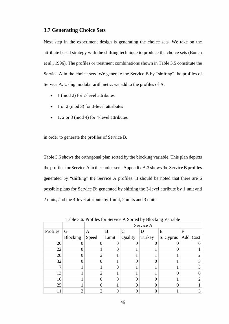
46
3.7 Generating Choice Sets
Next step in the experiment design is generating the choice sets. We take on the
attribute based strategy with the shifting technique to produce the choice sets (Bunch
et al., 1996). The profiles or treatment combinations shown in Table 3.5 constitute the
Service A in the choice sets. We generate the Service B by “shifting” the profiles of
Service A. Using modular arithmetic, we add to the profiles of A:
1 (mod 2) for 2-level attributes
1 or 2 (mod 3) for 3-level attributes
1, 2 or 3 (mod 4) for 4-level attributes
in order to generate the profiles of Service B.
Table 3.6 shows the orthogonal plan sorted by the blocking variable. This plan depicts
the profiles for Service A in the choice sets. Appendix A.3 shows the Service B profiles
generated by “shifting” the Service A profiles. It should be noted that there are 6
possible plans for Service B: generated by shifting the 3-level attribute by 1 unit and
2 units, and the 4-level attribute by 1 unit, 2 units and 3 units.
Table 3.6: Profiles for Service A Sorted by Blocking Variable
Service A
Profiles G A B C D E F
Blocking Speed Limit Quality Turkey S. Cyprus Add. Cost
20 0 0 0 0 0 0 0
22 0 1 0 1 1 0 1
28 0 2 1 1 1 1 2
32 0 0 1 0 0 1 3
7 1 1 0 1 1 1 3
13 1 2 1 1 1 0 0
16 1 0 0 0 0 1 2
25 1 0 1 0 0 0 1
11 2 2 0 0 0 1 3

47
12 2 0 1 1 1 0 1
14 2 0 0 1 1 1 2
21 2 1 1 0 0 0 0
8 3 2 0 0 0 0 1
9 3 0 0 1 1 0 0
10 3 0 1 1 1 1 3
18 3 1 1 0 0 1 2
3 4 1 0 0 1 0 3
4 4 0 0 1 0 0 2
17 4 0 1 1 0 1 1
19 4 2 1 0 1 1 0
1 5 0 0 1 0 1 0
2 5 2 1 0 1 0 2
5 5 1 0 0 1 1 1
24 5 0 1 1 0 0 3
6 6 0 0 0 1 1 0
15 6 0 1 0 1 0 3
23 6 1 1 1 0 0 2
29 6 2 0 1 0 1 1
26 7 0 1 0 1 1 1
27 7 2 0 1 0 0 3
30 7 1 1 1 0 1 0
31 7 0 0 0 1 0 2
At this point, let us investigate our design for the desired properties of an efficient
experimental design: orthogonality, level balance and minimal overlap. Our design
fulfills “orthogonality” because the profiles of Service A are generated as an
orthogonal design in the first place, and the shifting technique maintains the
orthogonality of Service B. This can be verified by adding up orthogonal codes of
columns to find each column sums up to zero. The “level balance” property refers to
having all the attribute levels show up the same number of times in the profiles. In our
design, each level appears 16 times for the 2-level attributes, 8 times for the 4-level
attribute, and 8 times for the two non-zero levels of the 3-level attribute (note that the
number of profiles is not divisible by 3, so this is the best that can be done for level
balance). Last, our design has also “minimal overlap” property as the shifting

48
technique to generate Service B ensures that no attribute is used more than once in
each choice set.
A fourth desirable property for design efficiency is “utility balance”. Utility balance is
maintained by reducing the utility gap among Service A and Service B in each choice
set. If the expected utility of the respondents from the alternatives is closer to each
other, the analyst is able to extract more information from the Choice Experiment. The
last column titled “Code-sum difference” in Appendix A.3 is included in order to
determine which of the 6 scenarios for Service B produce better utility balance, and
hence we can choose the most preferable Service B to use in our study.
Code-sum difference, as the name suggests, is the absolute difference between the sum
of codes in Service A and the sum of codes in Service B, for each choice set. The
higher the code for each attribute, the higher is the expected utility level from that
attribute, except the cost attribute. Therefore we add the negative of the level of the
cost attribute when calculating code-sums. By this way, we also make sure the higher
the code-sum for each alternative, the higher is the expected utility level for that
alternative. Thus, the code-sum difference between Services A and B gives us the
utility gap between A and B: the higher the code-sum difference the higher the utility
gap, and the lower the code-sum difference the lower the utility gap.
The above information tells us to look for the minimum code-sum differences in order
to have the best utility balance. Looking at Appendix A.3, we see that the Service B in
scenario 5 produces the minimum code-sum differences.

49
We choose to continue with the Service B in scenario 5. Table 3.7 depicts the final
versions of Service A and Service B in design codes. Table 3.8 depicts again Service
A and Service B in labelled attribute levels.

Table 3.7: Final Version of Service A and Service B in Design Codes
Service A Service B
Profil
es G A B C D E F A B C D E F
Code-sum
difference
Blocki
ng Speed Limit Quality Turkey
S.
Cyprus
Add.
Cost Speed Limit Quality Turkey
S.
Cyprus
Add.
Cost
20 0 0 0 0 0 0 0 1 1 1 1 1 3 0,5
22 0 1 0 1 1 0 1 2 1 0 0 1 0 2,5
28 0 2 1 1 1 1 2 0 0 0 0 0 1 4,5
32 0 0 1 0 0 1 3 1 0 1 1 0 2 2,5
7 1 1 0 1 1 1 3 2 1 0 0 0 2 0,5
13 1 2 1 1 1 0 0 0 0 0 0 1 3 8,5
16 1 0 0 0 0 1 2 1 1 1 1 0 1 4,5
25 1 0 1 0 0 0 1 1 0 1 1 1 0 4,5
11 2 2 0 0 0 1 3 0 1 1 1 0 2 1,5
12 2 0 1 1 1 0 1 1 0 0 0 1 0 0,5
14 2 0 0 1 1 1 2 1 1 0 0 0 1 0,5
21 2 1 1 0 0 0 0 2 0 1 1 1 3 1,5
8 3 2 0 0 0 0 1 0 1 1 1 1 0 3,5
9 3 0 0 1 1 0 0 1 1 0 0 1 3 3,5
10 3 0 1 1 1 1 3 1 0 0 0 0 2 1,5
18 3 1 1 0 0 1 2 2 0 1 1 0 1 2,5
3 4 1 0 0 1 0 3 2 1 1 0 1 2 4,5
4 4 0 0 1 0 0 2 1 1 0 1 1 1 4,5
17 4 0 1 1 0 1 1 1 0 0 1 0 0 0,5
19 4 2 1 0 1 1 0 0 0 1 0 0 3 8,5

1 5 0 0 1 0 1 0 1 1 0 1 0 3 3,5
2 5 2 1 0 1 0 2 0 0 1 0 1 1 0,5
5 5 1 0 0 1 1 1 2 1 1 0 0 0 2,5
24 5 0 1 1 0 0 3 1 0 0 1 1 2 2,5
6 6 0 0 0 1 1 0 1 1 1 0 0 3 3,5
15 6 0 1 0 1 0 3 1 0 1 0 1 2 2,5
23 6 1 1 1 0 0 2 2 0 0 1 1 1 2,5
29 6 2 0 1 0 1 1 0 1 0 1 0 0 0,5
26 7 0 1 0 1 1 1 1 0 1 0 0 0 0,5
27 7 2 0 1 0 0 3 0 1 0 1 1 2 1,5
30 7 1 1 1 0 1 0 2 0 0 1 0 3 5,5
31 7 0 0 0 1 0 2 1 1 1 0 1 1 4,5
Table 3.8: Final Version of Service A and Service B with Labelled Attribute Levels
Service A Service B
Profile
s G A B C D E F A B C D E F
Blocki
ng Speed Limit
Qualit
y
Turk
ey
S.
Cyprus
Add.
Cost Speed Limit
Qualit
y
Turk
ey
S.
Cyprus
Add.
Cost
20 0
Present
speed Limited
Present
level No No 20 TL
10 times
faster Unlimited
Better
quality Yes Yes 80 TL
22 0
10 times
faster Limited
Better
quality Yes No 40 TL
100 times
faster Unlimited
Present
level No Yes 20 TL
28 0
100 times
faster Unlimited
Better
quality Yes Yes 60 TL
Present
speed Limited
Present
level No No 40 TL
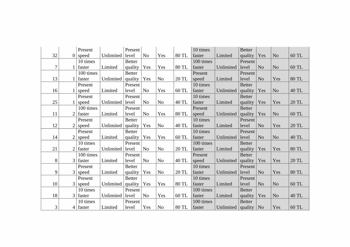
32 0
Present
speed Unlimited
Present
level No Yes 80 TL
10 times
faster Limited
Better
quality Yes No 60 TL
7 1
10 times
faster Limited
Better
quality Yes Yes 80 TL
100 times
faster Unlimited
Present
level No No 60 TL
13 1
100 times
faster Unlimited
Better
quality Yes No 20 TL
Present
speed Limited
Present
level No Yes 80 TL
16 1
Present
speed Limited
Present
level No Yes 60 TL
10 times
faster Unlimited
Better
quality Yes No 40 TL
25 1
Present
speed Unlimited
Present
level No No 40 TL
10 times
faster Limited
Better
quality Yes Yes 20 TL
11 2
100 times
faster Limited
Present
level No Yes 80 TL
Present
speed Unlimited
Better
quality Yes No 60 TL
12 2
Present
speed Unlimited
Better
quality Yes No 40 TL
10 times
faster Limited
Present
level No Yes 20 TL
14 2
Present
speed Limited
Better
quality Yes Yes 60 TL
10 times
faster Unlimited
Present
level No No 40 TL
21 2
10 times
faster Unlimited
Present
level No No 20 TL
100 times
faster Limited
Better
quality Yes Yes 80 TL
8 3
100 times
faster Limited
Present
level No No 40 TL
Present
speed Unlimited
Better
quality Yes Yes 20 TL
9 3
Present
speed Limited
Better
quality Yes No 20 TL
10 times
faster Unlimited
Present
level No Yes 80 TL
10 3
Present
speed Unlimited
Better
quality Yes Yes 80 TL
10 times
faster Limited
Present
level No No 60 TL
18 3
10 times
faster Unlimited
Present
level No Yes 60 TL
100 times
faster Limited
Better
quality Yes No 40 TL
3 4
10 times
faster Limited
Present
level Yes No 80 TL
100 times
faster Unlimited
Better
quality No Yes 60 TL

4 4
Present
speed Limited
Better
quality No No 60 TL
10 times
faster Unlimited
Present
level Yes Yes 40 TL
17 4
Present
speed Unlimited
Better
quality No Yes 40 TL
10 times
faster Limited
Present
level Yes No 20 TL
19 4
100 times
faster Unlimited
Present
level Yes Yes 20 TL
Present
speed Limited
Better
quality No No 80 TL
1 5
Present
speed Limited
Better
quality No Yes 20 TL
10 times
faster Unlimited
Present
level Yes No 80 TL
2 5
100 times
faster Unlimited
Present
level Yes No 60 TL
Present
speed Limited
Better
quality No Yes 40 TL
5 5
10 times
faster Limited
Present
level Yes Yes 40 TL
100 times
faster Unlimited
Better
quality No No 20 TL
24 5
Present
speed Unlimited
Better
quality No No 80 TL
10 times
faster Limited
Present
level Yes Yes 60 TL
6 6
Present
speed Limited
Present
level Yes Yes 20 TL
10 times
faster Unlimited
Better
quality No No 80 TL
15 6
Present
speed Unlimited
Present
level Yes No 80 TL
10 times
faster Limited
Better
quality No Yes 60 TL
23 6
10 times
faster Unlimited
Better
quality No No 60 TL
100 times
faster Limited
Present
level Yes Yes 40 TL
29 6
100 times
faster Limited
Better
quality No Yes 40 TL
Present
speed Unlimited
Present
level Yes No 20 TL
26 7
Present
speed Unlimited
Present
level Yes Yes 40 TL
10 times
faster Limited
Better
quality No No 20 TL
27 7
100 times
faster Limited
Better
quality No No 80 TL
Present
speed Unlimited
Present
level Yes Yes 60 TL
30 7
10 times
faster Unlimited
Better
quality No Yes 20 TL
100 times
faster Limited
Present
level Yes No 80 TL

31 7
Present
speed Limited
Present
level Yes No 60 TL
10 times
faster Unlimited
Better
quality No Yes 40 TL

55
3.8 Versions of Choice Sets
Profiles for the Service A and Service B in the choice sets are now final. The
experiment design is divided into 8 blocks of 4 profiles each, therefore each survey
respondent will be presented with 4 choice sets. These blocks constitute the versions
of the CE study. Table 3.9 displays the 8 versions.
Table 3.9: Versions of the Choice Experiment
Profile Version Choice Set
20 1 1
22 1 2
28 1 3
32 1 4
7 2 1
13 2 2
16 2 3
25 2 4
11 3 1
12 3 2
14 3 3
21 3 4
8 4 1
9 4 2
10 4 3
18 4 4
3 5 1
4 5 2
17 5 3
19 5 4
1 6 1
2 6 2
5 6 3
24 6 4
6 7 1
15 7 2
23 7 3
29 7 4
26 8 1
27 8 2
30 8 3
31 8 4

56
3.9 Randomizing Choice Sets
Last but not the least step in CE design is randomizing the choice sets.
The need for randomizing occurs for two reasons. For one, there could be “learning
effects” in a CE study. People’s responses to the choice sets early in the experiment
may be of poor quality since they are still learning how to relate the choice sets to
reality. For two, there could be “fatigue effects” in a CE study. People’s responses
towards the end of the experiment may deteriorate because they get tired of answering
the questions and would like to get to the end as quickly as possible. Therefore, if the
choice sets for each version are presented to all the respondents in the same order, then
the study will be prone to “order bias”.
Completely randomizing the order of the choice sets is one option, however it would
require too many versions of the survey and make the administration of the CE study
very difficult. Instead, we duplicate each version of the survey by switching the order
of the first two choice sets and the last two choice sets. For instance, for the survey
version 1, we create two versions 1a and 1b. Version 1a, has the first two choice sets
(20, 22) and the last two choice sets (28, 32). This order is reversed in version 1b; the
first two choice sets are (28, 32) and the last two choice sets are (20, 22). The complete
list of 16 randomized versions of the survey is given in Table 3.10.
Table 3.10: Complete List of Randomized CE Versions
Version Choice Set Profile Version Choice Set Profile
1a 1 20 1b 1 28
1a 2 22 1b 2 32
1a 3 28 1b 3 20
1a 4 32 1b 4 22
2a 1 7 2b 1 16
2a 2 13 2b 2 25

57
2a 3 16 2b 3 7
2a 4 25 2b 4 13
3a 1 11 3b 1 14
3a 2 12 3b 2 21
3a 3 14 3b 3 11
3a 4 21 3b 4 12
4a 1 8 4b 1 10
4a 2 9 4b 2 18
4a 3 10 4b 3 8
4a 4 18 4b 4 9
5a 1 3 5b 1 17
5a 2 4 5b 2 19
5a 3 17 5b 3 3
5a 4 19 5b 4 4
6a 1 1 6b 1 5
6a 2 2 6b 2 24
6a 3 5 6b 3 1
6a 4 24 6b 4 2
7a 1 6 7b 1 23
7a 2 15 7b 2 29
7a 3 23 7b 3 6
7a 4 29 7b 4 15
8a 1 26 8b 1 30
8a 2 27 8b 2 31
8a 3 30 8b 3 26
8a 4 31 8b 4 27
3.10 Constructing the Survey Instrument
Finally, “Current Service” is added to every choice set as a third alternative in addition
to Service A and Service B. This makes the CE study more realistic for the respondent,
and enables her to relate the attributes of A and B to the current mobile service she is
using. If she does not find the Services A and B attractive, she has the option of staying
with her current service. The current service has the following attribute levels, for all
the respondents:

58
1. Current service internet speed: Present speed (The only mobile technology currently
available in TRNC is 3G)
2. Current service internet limit: Limited/meter-rate (Current GSM operators in TRNC
have no plans or packages which offer unlimited mobile internet use)
3. Current service internet quality: Present level
4. Use in Turkey w/out roaming cost with current service: No
5. Use in South Cyprus w/out roaming cost with current service: No
6. Additional monthly cost: 0 TL (No additional cost because it’s the current service)
Table 3.11 shows a sample choice set from the survey.
Table 3.11: A Sample Choice Set
Version 2a Choice Set 1
Service A Service B Service C
(Current
Service)
Internet speed 10 times faster 100 times faster Present speed
Internet limit Limited Unlimited Limited
Quality (speaking and internet) Better quality Present level Present level
Turkey w/out add.expenses Yes No No
S.Cyprus w/out add.expenses Yes No No
Additional monthly GSM cost 80 TL 60 TL 0 TL
Your Choice [ ] [ ] [ ]

59
Chapter 4
4 SURVEY DESIGN AND ADMINISTRATION
4.1 Introduction
In the last chapter, we established the design for the choice experiment, and produced
the choice questions to be included in the survey. In Chapter 4, we move on to the
contents of the questionnaire and to the administration of the survey.
4.2 Survey Sections
The survey consists of 5 sections in total. Two of these sections are devoted to
extracting the data for the CVM (Contingent Valuation Method) and the CE (Choice
Experiment) studies. Two other sections collect background information about the
respondents, regarding their mobile experience and their demographic characteristics.
The last section is spared for the interviewer’s use in order to rate the quality of the
interview.
The first section is titled “Mobile Phone and Internet Use” and includes questions to
gather data on the respondent’s mobile experience. These questions collect
information such as the type of mobile devices owned, the monthly amount paid for
mobile services, the frequency of mobile internet use, the purposes for mobile internet
use, and the type of mobile internet plan. These questions are followed by additional
questions about the respondent’s use of mobile services abroad. The survey
specifically asks for the frequency of travel to Turkey and South Cyprus, and the
respondent’s desire to use her local plan in these two destinations.

60
The second section is the CVM section. This is where we directly ask the respondent
to state her willingness to pay for 4G service. In this section, we first present the
interviewee with a detailed description of what 4G is, and what benefits 4G has over
3G. This is done in order to ensure the interviewee is as informed as possible, when
stating her WTP. The CVM question is asked in the ‘payment ladder’ format. In this
format, the respondent is presented with a ladder of prices, and she is asked to mark
the highest amount she would pay for 4G, and the first (lowest) amount she would not
pay. The first stands for her minimum WTP, and the latter for her maximum WTP.
Therefore, we obtain an interval where the observer’s true WTP lies. It should be noted
that the payment ladder approach is preferable to an open-ended question. In the open-
ended elicitation technique, many respondents may prefer not to answer due to the lack
of a benchmark, and also, some may answer strategically making this technique prone
to strategic bias.
The next section is the Choice Experiment section. There are 16 different versions of
this section as described in Chapter 3, section 3.9. Each respondent is given a set of 4
choice questions similar to that in Table 3.11. The interviewers are trained beforehand
to assist the respondents with answering choice questions without affecting their
responses.
The fourth section is titled “Demographic Questions” and this is where we extract the
respondents’ demographic characteristics. The information we gather include age,
gender, education, employment and net monthly income.
The last section is for interviewer use only. The interviewer rates the interview on a
scale of very poor to very good. The interviewer considers the concentration of the

61
interviewee and the quality of her understanding of the survey, while doing the rating.
A copy of the complete survey is given in Appendix B.
4.3 Sample Size
Orme (2006) suggests a rule of thumb to determine the minimum sample size required
to study choice based data. According to this rule, the minimum number of respondents
𝑛 can be calculated as follows:
𝑛𝑡𝑎
𝑐> 500
where 𝑡 is the number of choice sets answered by each respondent, 𝑎 is the number of
alternatives in every choice set not including the current alternative, and 𝑐 is the largest
number of levels in the attributes (for designs not considering interaction effects). In
our case, 4 choice sets are given to each respondent, there are 2 alternatives in each
choice set, and 4 is the largest number of levels in the attributes. The calculations lead
to a figure of 250 as the minimum sample size required. Orme (2006) adds that a
minimum of 300 respondents is advisable for quantitative studies, so we determine our
sample size to be 320. Since we have 16 versions of the choice experiment, we allocate
20 respondents for each version.
Louviere et al. (2000) gives another method for calculating total sample size in a
choice experiment:
𝑛 ≥(1−𝑝)
𝑟𝑝𝑎2𝛷−1(
1+𝛼
2)
where 𝑝 is the true choice probability (true population proportion), 𝑟 is the number of
choice sets that each individual respondent is given, 𝛷−1(⋅) is the inverse cumulative
normal distribution function, and we wish to estimate the true population proportion
within 𝑎 per cent of the true value 𝑝 with probability 𝛼 or greater. Taking 𝑝 = 0.5,

62
𝑟 = 4, 𝑎 = 10% and 𝛼 = 0.95, we calculate 𝑛 ≥ 96. Therefore, our choice of 320
respondents is a satisfactory sample size.
4.4 Sampling Method
Once we decide on the sample size, the next task is to identify the relevant (target)
population. The relevant population is determined by the objectives of the study. In
our study, we aim to quantify the value of improvements in mobile services, so our
target group is the users of mobile services. Therefore, we choose to admit respondents
to our survey by one question: Do you purchase mobile service for personal use? In
the case of North Cyprus, this amounts to an overwhelming majority of the total
population above 18 years of age.
Next, we pick the sampling method, which we will use to choose the individuals to be
included in the survey sample. According to Champ et al. (2003), there are two types
of sampling techniques: non-probability sampling and probability sampling. Non-
probability sampling refers to when there is no known probability that any member of
the population will be included in the sample. We cannot use the sample’s results to
make statistical inferences for the population. Probability sampling, on the other hand,
refers to when the probability of each individual being in the sample is known, so the
results of the survey can be used to infer for the population.
Louviere et al. (2000) lists the ‘probability sampling’ methods as follows: choice based
sampling (CBS), simple random sampling (SRS) and exogenously stratified random
sampling (ESRS). CBS requires the observation of choices made by the population. It
is mostly used in revealed preference studies, and not suitable for stated choice
experiments. SRS is where a random sample is picked from the population, and all

63
individuals in the population have the same chances of being selected to the sample.
ESRS, on the other hand, divides the population into mutually exclusive strata, and
performs random sampling within each stratum. The number of sample units to be
chosen from each stratum is in proportion with the relative sizes of the strata.
In our study, we prefer to have a fair representation from all regions of North Cyprus.
Therefore, we opt to use exogenously stratified random sampling (ESRS), with the
strata being the 5 districts of North Cyprus. We use the latest census data (2013) to
calculate the number of respondents to be picked from each district, as shown in Table
4.1.
Table 4.1: ESRS Sampling according to Districts
District Population % of Total Target number of
respondents
Lefkoşa 94,824 33% 106
Gazimağusa 69,741 24% 78
Girne 69,163 24% 77
Güzelyurt 30,037 10% 34
İskele 22,492 8% 25
Total 286,257 100% 320
4.5 Questionnaire Results
The survey was conducted in March 2015 by a professional polling firm, Prologue
Consulting Ltd. A total of 320 individuals were interviewed in all five districts of
North Cyprus. Random sampling was performed within each district, reflecting the
characteristics of the population with reasonable accuracy.
In-person interviewing was used as the survey administration mode, because the
concepts in the study are fairly complicated and respondents may need guidance in
answering choice questions. The concepts and attributes were explained thoroughly in

64
a document preceding the section containing the choice questions. As described in
section 4.1, the survey included a section that elicits information from respondents
about their experience with mobile services, and a section that collects demographic
data. Table 4.2 below presents a summary of this data.
Table 4.2: Questionnaire Results
Variable No.
obs.
Mean /
% Std dev.
Min
.
25th
%tile
Med
ian
75th
%tile Max.
Mobile exp. & travel
data
Mobile device
ownership 320
Regular mobile
phone 68 21%
Smart phone 283 88%
Tablet 76 24%
Laptop 144 45%
Mobile
subscription 320
I have 320 100%
I do not have 0 0%
Mobile subs.
expenditure
(TL/month) 320 107.23 91.98 20 50 80 130 800
Frequency of
mobile int.use 320
Every day 221 69%
Several times a
week 61 19%
Several times a
month 4 1%
Very rarely 3 1%
Never 31 10%
Purpose for mobile
int. use 288
Search engines 172 60%
E-mail 100 35%
Instant messaging 190 66%
Voice over IP 97 34%
Videophone 72 25%
Social
networking sites 255 89%
News sites 175 61%
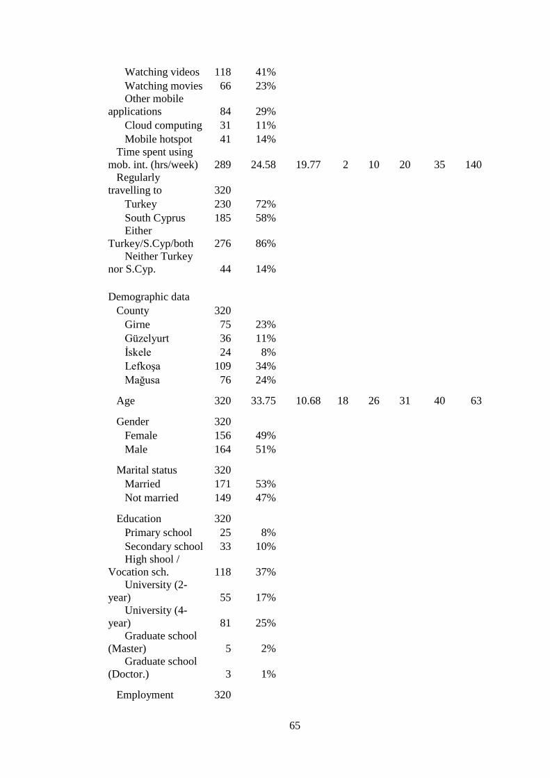
65
Watching videos 118 41%
Watching movies 66 23%
Other mobile
applications 84 29%
Cloud computing 31 11%
Mobile hotspot 41 14%
Time spent using
mob. int. (hrs/week) 289 24.58 19.77 2 10 20 35 140
Regularly
travelling to 320
Turkey 230 72%
South Cyprus 185 58%
Either
Turkey/S.Cyp/both 276 86%
Neither Turkey
nor S.Cyp. 44 14%
Demographic data
County 320
Girne 75 23%
Güzelyurt 36 11%
İskele 24 8%
Lefkoşa 109 34%
Mağusa 76 24%
Age 320 33.75 10.68 18 26 31 40 63
Gender 320
Female 156 49%
Male 164 51%
Marital status 320
Married 171 53%
Not married 149 47%
Education 320
Primary school 25 8%
Secondary school 33 10%
High shool /
Vocation sch. 118 37%
University (2-
year) 55 17%
University (4-
year) 81 25%
Graduate school
(Master) 5 2%
Graduate school
(Doctor.) 3 1%
Employment 320

66
Employed 226 71%
Unemployed/out
of labour 94 29%
Net monthly
income (TL/month) 269
2,504.4
1
1,557.5
0 300
1,60
0
2,00
0 3,000
11,00
0

67
Chapter 5
5 CHOICE EXPERIMENT RESULTS
5.1 Revisiting the CE Model
As described in Chapter 2, CE methodology makes use of the random utility theory.
An individual, when faced with an alternative 𝑖, derives a utility from this alternative
as follows:
𝑈𝑖 = 𝑉𝑖 + 𝜀𝑖
The component 𝑉𝑖 is observable to the researcher, and the random component 𝜀𝑖 is not.
The observed component 𝑉𝑖 is where the set of attributes that are observable and
measurable reside. The simplest assumption for 𝑉𝑖 would be that it is a linear function
of the attributes, each of which is weighted by a unique weight to account for that
attribute’s marginal utility input. Using 𝑓 as a generalized notation for functional form,
but noting that the functional form can be different for each attribute, we can write 𝑉𝑖
as:
𝑉𝑖 = 𝛽0𝑖 + 𝛽1𝑖𝑓(𝑋1𝑖) + 𝛽2𝑖𝑓(𝑋2𝑖) + 𝛽3𝑖𝑓(𝑋3𝑖) + ⋯ + 𝛽𝐾𝑖𝑓(𝑋𝐾𝑖)
where 𝑋𝑘𝑖 represents the 𝑘 = 1 to 𝐾 attributes of alternative 𝑖, 𝛽𝑘𝑖 represents the
weights of these attributes, and 𝛽0𝑖 is a parameter that is not associated with any
observed attribute, but represents the role of all unobserved sources of utility.
We treat each attribute in our study to be linear so that 𝑓(𝑋) = 𝑋; we assume the
random component of utility 𝜀𝑖 to be inclusive of all sources of variance from

68
unobserved components of 𝛽 and 𝑋, and also that 𝜀𝑖 is IID (independently and
identically distributed). We end up with the multinomial logit (MNL) model:
𝑈 = 𝐴𝑆𝐶 + 𝛽𝑓𝑎𝑠𝑡𝑋𝑓𝑎𝑠𝑡 + 𝛽𝑣𝑒𝑟𝑦𝑓𝑎𝑠𝑡𝑋𝑣𝑒𝑟𝑦𝑓𝑎𝑠𝑡 + 𝛽𝑢𝑛𝑙𝑖𝑚𝑖𝑡𝑒𝑑𝑋𝑢𝑛𝑙𝑖𝑚𝑖𝑡𝑒𝑑 +
𝛽𝑞𝑢𝑎𝑙𝑖𝑡𝑦𝑋𝑞𝑢𝑎𝑙𝑖𝑡𝑦 + 𝛽𝑡𝑢𝑟𝑘𝑒𝑦𝑋𝑡𝑢𝑟𝑘𝑒𝑦 + 𝛽𝑠𝑜𝑢𝑡ℎ𝑐𝑦𝑝𝑟𝑢𝑠𝑋𝑠𝑜𝑢𝑡ℎ𝑐𝑦𝑝𝑟𝑢𝑠 + 𝛽𝑝𝑟𝑖𝑐𝑒𝑋𝑝𝑟𝑖𝑐𝑒 + 𝜀
The alternative-specific constant (𝐴𝑆𝐶) represents the utility derived from the existing
service, and it captures the real and psychological costs of switching to a new service.
The attribute variables 𝑋, except for the price attribute, are binary variables taking on
the value 1 when the attribute is present in the service and 0 if it is not present. It should
also be noted that we split the attribute for mobile internet speed into two attributes:
fast speed and very fast speed. This is because we would like to detect the non-linear
impact of moving from the present speed (3 Mbps) to 10 times faster (30 Mbps), and
also from 10 times faster (30 Mbps) to 100 times faster (300 Mbps).
As the form of the utility expression is identified, we turn to how an individual makes
a choice in a CE. The individual faces 𝑗 = 1 to 𝐽 alternatives, where 𝐽 = 3 in our
survey. In order to make a choice, the individual will evaluate the utility she or he will
derive for each alternative and pick the one with the highest utility. Putting this into
notation, the probability that alternative 𝑖 will be chosen is:
𝑃𝑖 = 𝑃 ((𝑈𝑖 ≥ 𝑈𝑗) ∀ 𝑗 ∈ 𝑗 = 1, … , 𝐽; 𝑖 ≠ 𝑗)
Rearranging gives us:
𝑃𝑖 = 𝑃 ((𝑉𝑖 + 𝜀𝑖 ≥ 𝑉𝑗 + 𝜀𝑗) ∀ 𝑗 ∈ 𝑗 = 1, … , 𝐽; 𝑖 ≠ 𝑗)
𝑃𝑖 = 𝑃 (((𝜀𝑗 − 𝜀𝑖) ≤ (𝑉𝑖 − 𝑉𝑗)) ∀ 𝑗 ∈ 𝑗 = 1, … , 𝐽; 𝑖 ≠ 𝑗)
Since the left-hand side of the inequality is not observable, estimating the model
requires picking up a probability distribution for the ‘error term’. A popular

69
distribution in discrete choice analysis is the extreme value type 1 (EV1) distribution,
which has the following form:
𝑃(𝜀𝑗 ≤ 𝜀) = exp(− exp −𝜀)
Equipped with the IID and EV1 assumptions, we proceed to complete the model.
Louviere et al. (2000, Chapter 3) took on the full derivation of the MNL model, and
ended with the following:
𝑃𝑖 =exp 𝑉𝑖
∑ exp 𝑉𝑗𝐽𝑗=1
; 𝑗 = 1, … , 𝑖, … , 𝐽 𝑖 ≠ 𝑗
In words, this states that the probability of an individual choosing alternative 𝑖 out of
𝐽 alternatives is equal to the ratio of the exponential of the observed utility index for
alternative 𝑖 to the sum of the exponentials of the observed utility indices for all 𝐽
alternatives including the 𝑖th alternative.
5.2 Estimating the Model
Our model can be estimated using maximum likelihood techniques. Letting 𝐼𝑛𝑗 be a
dummy variable that takes value 1 if individual 𝑛 chooses the alternative 𝑗 and 0
otherwise, the log-likelihood function of the model for a total number of respondents
𝑁 is given by:
ln 𝐿 = ∑ ∑ 𝐼𝑛𝑗 ln 𝑃𝑛𝑗
𝐽
𝑗=1
𝑁
𝑛=1
The parameters to be estimated are the weights 𝛽 of the attributes in the utility function,
and these can be estimated by maximizing the log-likelihood function above (it should
be noted that the weights 𝛽 reside inside the term 𝑃𝑛𝑗). Once 𝛽 are estimated, we can
calculate the WTP figures. Since 𝑋 consists of 𝐾 = 7 attributes and one of the

70
attributes is the price attribute 𝑝, the marginal willingness to pay (MWTP) for a change
in the level of one attribute 𝑘 and the willingness to pay (WTP) for the whole service
in question resulting from changes in the levels of all the attributes can be calculated
as shown by Lancsar and Savage (2004):
𝑀𝑊𝑇𝑃𝑘 =
𝑑𝑉
𝑑𝑋𝑘
−𝑑𝑉
𝑑𝑝
=𝛽𝑘
−𝛽𝑝
𝑊𝑇𝑃 = ∑𝛽𝑘
𝛽𝑝(𝛥𝑋𝑘)𝐾
𝑘=1
5.3 Results
5.3.1 The Goodness of Fit of the Model
The MNL model is estimated using NLOGIT v5.0 software package. In order to
determine the goodness of fit of the estimated model, we compare it to the constants-
only model using the likelihood-ratio (LL-ratio) test. LL for our model was computed
as −1,154.13, and LL for the constants-only model as −1,340.89. The LL-ratio test is
given as follows:
−2 ∗ (𝐿𝐿 𝑐𝑜𝑛𝑠𝑡𝑎𝑛𝑡𝑠 𝑜𝑛𝑙𝑦 𝑚𝑜𝑑𝑒𝑙 − 𝐿𝐿 𝑒𝑠𝑡𝑖𝑚𝑎𝑡𝑒𝑑 𝑚𝑜𝑑𝑒𝑙) ~ 𝑐ℎ𝑖 𝑠𝑞𝑢𝑎𝑟𝑒
For our model,
−2𝐿𝐿 = −2(−1340.89 − (−1154.13)) = 373.52
The critical value of chi square at 95% significance level with d.f. 7 (degrees of
freedom for the test is the difference in the number of estimated parameters in the two
models = 8 – 1 = 7) is 14.07. The LL-ratio test result, 373.52, is larger than this chi-
critical, so we reject the null hypothesis that the estimated model is not better than the
constants-only model.
5.3.2 Results of MNL Estimation
The results of the model estimation are presented in Table 5.1.

71
Table 5.1: Results of MNL Model Estimation
Variables β-coefficient Standard Error
95% Confidence
Interval
ASC −.59350*** .16673 −.92029 −.26671
FAST .63411*** .11140 .41578 .85245
VERYFAST .71585*** .12728 .46638 .96531
UNLIMITED .25375*** .08938 .07857 .42893
QUALITY −.15118*** .08865 −.32494 .02257
TURKEY .92894*** .09394 .74482 1.11307
SOUTHCYPRUS .61745*** .09041 .44025 .79465
PRICE −.03141*** .00234 −.03599 −.02683
Note: ***, **, * indicate statistical significance at the 1%, 5%, 10% levels,
respectively.
All the estimated coefficients for the attributes in the utility function are significant at
the 1% level, except the coefficient for the quality attribute. The coefficient of quality
is statistically insignificant at the 1% and 5% levels, and its 95% confidence interval
contains zero. We conclude that the study finds no evidence that an improved quality
of mobile services will enhance consumers’ utility.
The signs of the estimated coefficients are consistent with our expectations (again,
except for the quality attribute, which we already accepted to be statistically
insignificant). Attributes for fast speed, very fast speed, unlimited internet,
unrestrained use in Turkey and unrestrained use in South Cyprus all have a positive
impact on consumers’ utility, whereas price has a negative impact. The estimated
coefficient for unrestrained use in Turkey is the greatest, which implies that this is the
attribute that improves consumers’ utility the most. Coefficients for very fast speed,
fast speed, unrestrained use in South Cyprus, and unlimited internet use follow,
respectively.
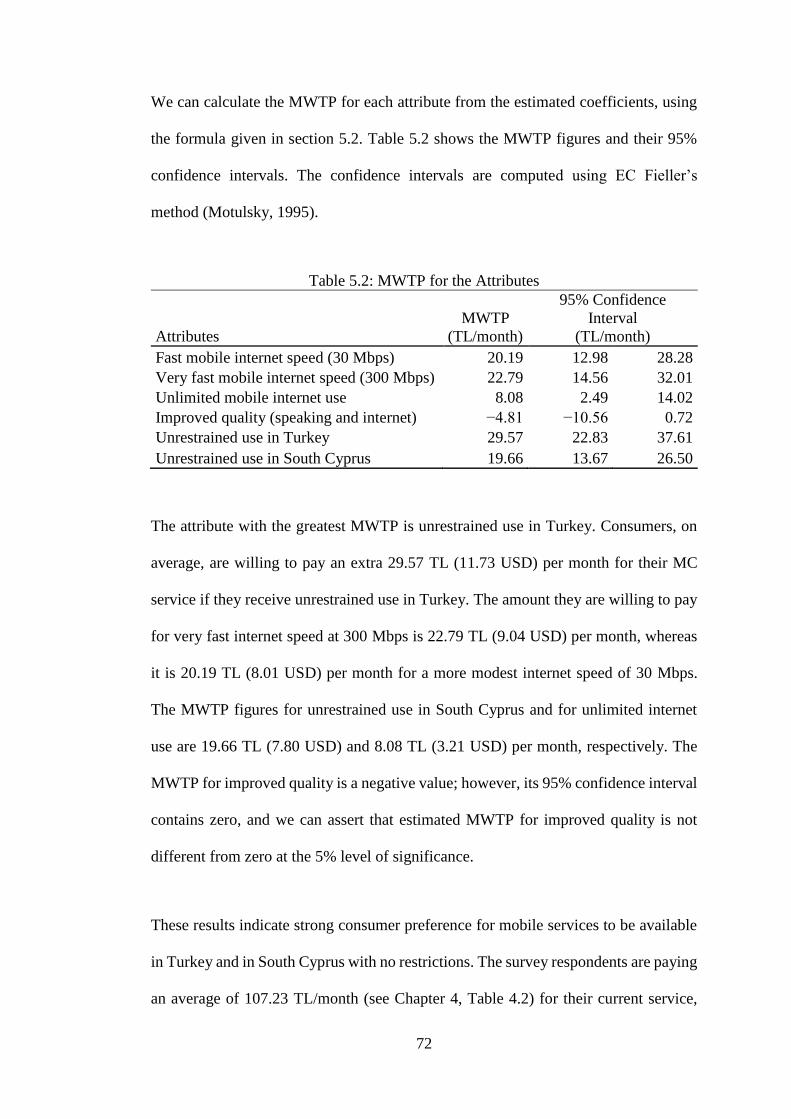
72
We can calculate the MWTP for each attribute from the estimated coefficients, using
the formula given in section 5.2. Table 5.2 shows the MWTP figures and their 95%
confidence intervals. The confidence intervals are computed using EC Fieller’s
method (Motulsky, 1995).
Table 5.2: MWTP for the Attributes
Attributes
MWTP
(TL/month)
95% Confidence
Interval
(TL/month)
Fast mobile internet speed (30 Mbps) 20.19 12.98 28.28
Very fast mobile internet speed (300 Mbps) 22.79 14.56 32.01
Unlimited mobile internet use 8.08 2.49 14.02
Improved quality (speaking and internet) −4.81 −10.56 0.72
Unrestrained use in Turkey 29.57 22.83 37.61
Unrestrained use in South Cyprus 19.66 13.67 26.50
The attribute with the greatest MWTP is unrestrained use in Turkey. Consumers, on
average, are willing to pay an extra 29.57 TL (11.73 USD) per month for their MC
service if they receive unrestrained use in Turkey. The amount they are willing to pay
for very fast internet speed at 300 Mbps is 22.79 TL (9.04 USD) per month, whereas
it is 20.19 TL (8.01 USD) per month for a more modest internet speed of 30 Mbps.
The MWTP figures for unrestrained use in South Cyprus and for unlimited internet
use are 19.66 TL (7.80 USD) and 8.08 TL (3.21 USD) per month, respectively. The
MWTP for improved quality is a negative value; however, its 95% confidence interval
contains zero, and we can assert that estimated MWTP for improved quality is not
different from zero at the 5% level of significance.
These results indicate strong consumer preference for mobile services to be available
in Turkey and in South Cyprus with no restrictions. The survey respondents are paying
an average of 107.23 TL/month (see Chapter 4, Table 4.2) for their current service,

73
and are willing to accept a 28% increase in their monthly mobile bill for unrestrained
roaming in Turkey and an 18% increase for the same in South Cyprus. One reason that
roaming in Turkey is valued higher than that in South Cyprus could be that citizens of
North Cyprus travel to South Cyprus by car mostly for day trips, whereas they take a
flight to visit Turkey and stay longer. It could be argued that consumers can handle
missing out on mobile services for short periods, but not for longer trips. Therefore,
an individual who travels to both destinations may value free roaming more in Turkey
than in South Cyprus. An additional factor is that the number of survey respondents
regularly traveling to Turkey is larger than the number regularly traveling to South
Cyprus. 230, out of the 320 surveyed, report that Turkey is a regular destination,
whereas 185 report the same for South Cyprus (see Chapter 4, Table 4.2). Since more
people need mobile services in Turkey, the average MWTP for Turkish roaming rises.
It should be further noted from the survey statistics in Table 4.2, that 276 respondents,
or 86% of the surveyed, travel to either or both of the two destinations, which explains
why people are interested in unrestrained roaming so much.
The results of the study also suggest that there is substantial demand for the upgrade
of mobile services in North Cyprus to the 4G grade, with unlimited use if possible.
Consumers are willing to pay 19% to 21% more than they currently pay in order to
have faster 4G-rate connection speeds, and 8% more in order to receive unlimited
mobile internet use. These results are in line with the survey statistics (Table 4.2),
which show that consumers are already using data-intensive mobile applications such
as social networking (89%), instant messaging (66%) and watching videos (41%).
Faster data rates will enhance consumers’ mobile experience.
74
Chapter 6
6 CVM RESULTS
6.1 Introduction
The second section of the survey is devoted to the Contingent Valuation Method
(CVM) study. As described in detail in Chapter 2, CVM asks the respondents to state
their willingness to pay directly, as opposed to having them make choices and inferring
their WTP from these choices.
The section starts with a description of the Fourth Generation (4G) mobile technology.
This is intended so that the respondents are as informed as possible, while stating their
WTP for 4G. According to this description, 4G enables both high-quality voice
conversation and very high speed mobile internet connectivity, easily in the range of
30 Mbps, whereas 3G offers a data rate of about 3 Mbps. The benefits of 4G are listed
as follows:
Mobile “videophone” conversations can be made.
Videos and movies on the internet will display instantly.
Real-time games on the internet can be played while mobile.
No freezing/disconnection in the video/movie/game stream while on the move.
(e.g. travelling in a car)
Very large file transfers can be made instantly over the internet.

75
Cloud computing can be used while mobile. With the very high speed mobile
internet connectivity, all personal files can be stored on the internet and
displayed on all personal mobile devices.
Because 4G mobile internet service can be used for home internet connection
as well, you may opt not to purchase a separate home internet service.
The descriptive introduction also states that another advantage of the 4G technology
when compared with 3G, is that 4G is better in quality. In other words 4G provides a
higher quality voice conversation and mobile internet connection capability, as 4G
users never experience any freezing or disconnection while speaking on their mobile
phone or surfing the internet.
Then, the respondents are asked to state their WTP, as an additional cost on their
current mobile expenditure, for a “4G service which provides mobile internet speed 10
times faster than 3G, unlimited internet use, and no freezing/disconnection in speaking
or internet connectivity”. The CVM question is asked in the ‘payment ladder’ format.
In this format, the respondents are presented with a ladder of prices, and they are
required to tick the highest amount they would pay for 4G, and to cross the first
(lowest) amount they would not pay. The tick stands for the minimum WTP, and the
cross stands for the maximum WTP. Therefore, we obtain an interval where the
respondent’s true WTP lies. It should be noted that the payment ladder approach is
preferable to an open-ended question because the open-ended elicitation technique is
prone to non-responses and to strategic bias as mentioned in Section 4.2.

76
6.2 Data
All 320 respondents of the survey answered the CVM section. Of these 320, 26 stated
that they would not go for 4G (i.e., their WTP is nil). These respondents were further
required to state the reason(s) why they would not go for 4G. Table 6.1 presents the
list and the frequency of the reasons given.
Table 6.1: Reasons for Zero WTP
# Reason Frequency
1 3G is good enough/do not need 4G 12
2 Do not need to use mobile internet 6
3 Do not know how to use internet 3
4 4G should be introduced without extra cost 2
5 3G is bad, 4G is even worse (?) 1
6 Prefers to use WiFi instead of 3G/4G 1
7 No specific reason 1
Total 26
Reason #4 is considered to be a protest response, since it does not necessarily imply
that the respondent puts zero value on a 4G service. Therefore we remove these 2
protest responses from the CVM study, so as to avoid a bias due to invalid zero bids.
We are left with 318 observations, 24 of which are true zero WTP bids, and the
remaining 194 are non-zero bids. Table 6.2 shows the frequencies for the ticks and for
the crosses provided by the survey takers.
Table 6.2: Frequencies of Ticks and Crosses
Bid
(TL)
Ticks
(lower bound of WTP)
Crosses
(higher bound of WTP)
0 24 24
5 47 0
10 66 14
15 50 25
20 56 36
25 37 47
30 18 42
40 9 46

77
50 8 45
70 2 28
100 0 9
150 1 0
200 0 2
300 0 0
Total 318 318
6.3 Turnbull Lower Bound Mean for WTP
If we use a parametric approach to estimate the WTP using the CVM data, we need to
make a distributional assumption. The estimated result is not robust against
distributional misspecification. Therefore, we opt to take a non-parametric approach
to estimating the mean WTP for 4G.
The first non-parametric estimate we take on is the Turnbull Lower Bound Mean
(LBM), suggested by Turnbull (1976). Turnbull LBM is known to be a conservative
WTP estimate, because it utilises only the lower bound information (the ‘ticks’) from
the CVM survey. As the first step, we take the tick data from Table 6.2, remove the
zero frequency bids, and calculate the cumulative number and proportion of ticks for
each bid. This is given in Table 6.3. The empirical survivor function is graphed in
Figure 6.1.
Table 6.3: Cumulative Number and Proportion of Ticks
i Bid (Bi) Number
of ticks
Cumulative
number of
ticks
Cumulative
proportion of ticks
(pi)
1 0 24 318 100,00%
2 5 47 294 92,45%
3 10 66 247 77,67%
4 15 50 181 56,92%
5 20 56 131 41,19%
6 25 37 75 23,58%
7 30 18 38 11,95%

78
8 40 9 20 6,29%
9 50 8 11 3,46%
10 70 2 3 0,94%
11 150 1 1 0,31%
12 200 0 0 0,00%
Figure 6.1: The Empirical Survivor Function
The steps to calculate the Turnbull LBM mean is given by Haab and McConnell
(1997). The formula for the mean is given as:
𝐿𝐵𝑀(𝑇𝑢𝑟𝑛𝑏𝑢𝑙𝑙) = 𝑝1𝐵1 + ∑ 𝑝𝑖(𝐵𝑖 − 𝐵𝑖−1)𝑚
𝑖=2
where 𝑚 is the total number of bids. The formula for the variance of the LBM is given
as:
𝑉𝑎𝑟(𝐿𝐵𝑀) = ∑𝑝𝑖(1 − 𝑝𝑖)(𝐵𝑖 − 𝐵𝑖−1)2
𝑁
𝑚
𝑖=1
where 𝑁 is the total number of observations (which is 318 in our study).
Table 6.4 shows the calculation of Lower Bound Mean, and the variance of LBM.
0%
10%
20%
30%
40%
50%
60%
70%
80%
90%
100%
0 25 50 75 100 125 150 175 200
Cu
mu
lati
ve p
rop
ort
ion
of
tick
s
Bid
Empirical Survivor Function
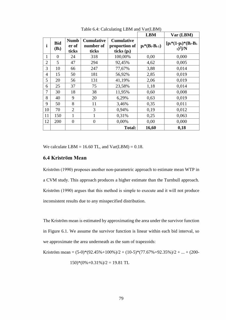
79
Table 6.4: Calculating LBM and Var(LBM)
LBM Var (LBM)
i Bid
(Bi)
Numb
er of
ticks
Cumulative
number of
ticks
Cumulative
proportion of
ticks (pi)
pi*(Bi-Bi-1) [pi*(1-pi)*(Bi-Bi-
1)2]/N
1 0 24 318 100,00% 0,00 0,000
2 5 47 294 92,45% 4,62 0,005
3 10 66 247 77,67% 3,88 0,014
4 15 50 181 56,92% 2,85 0,019
5 20 56 131 41,19% 2,06 0,019
6 25 37 75 23,58% 1,18 0,014
7 30 18 38 11,95% 0,60 0,008
8 40 9 20 6,29% 0,63 0,019
9 50 8 11 3,46% 0,35 0,011
10 70 2 3 0,94% 0,19 0,012
11 150 1 1 0,31% 0,25 0,063
12 200 0 0 0,00% 0,00 0,000
Total: 16,60 0,18
We calculate LBM = 16.60 TL, and Var(LBM) = 0.18.
6.4 Kriström Mean
Kriström (1990) proposes another non-parametric approach to estimate mean WTP in
a CVM study. This approach produces a higher estimate than the Turnbull approach.
Kriström (1990) argues that this method is simple to execute and it will not produce
inconsistent results due to any misspecified distribution.
The Kriström mean is estimated by approximating the area under the survivor function
in Figure 6.1. We assume the survivor function is linear within each bid interval, so
we approximate the area underneath as the sum of trapezoids:
Kriström mean = (5-0)*(92.45%+100%)/2 + (10-5)*(77.67%+92.35%)/2 + ... + (200-
150)*(0%+0.31%)/2 = 19.81 TL

80
6.5 Upper Bound Mean
Vaughan and Rodriguez (2001) demonstrate a procedure to calculate an Upper Bound
Mean for WTP, similar to the procedure for calculating the Turnbull Lower Bound
Mean:
𝑈𝐵𝑀 = ∑ 𝑝𝑖(𝐵𝑖+1 − 𝐵𝑖)𝑚
𝑖=1
Taking on the calculation:
UBM = (5-0)*100% + (10-5)*92.45% + ... + (200-150)*0.31% = 23.02 TL
Therefore, the estimated non-parametric means for the WTP of a 30 Mbps 4G service
can be ordered as follows:
Turnbull Lower Bound Mean (16.60 TL) < Kriström mean (19.81 TL) < Upper Bound
Mean (23.02 TL)
6.6 Sensitivity Analysis
Having calculated the WTP means estimated by the CVM methodology, we turn to
analysing the sensitivity of the WTP to mobile use frequency and demographic
characteristics of the respondents.
For this purpose, we estimate an empirical model for the maximum WTP for 4G, which
depends in turn on the following explanatory variables: mobile use frequency (hours
per week), age, gender, education (years of schooling) and income (net monthly
income in Turkish Liras). We use the lower bound information (the ‘ticks’ from the
CVM question) for the WTP data, and the answers to the survey questions for the
explanatory variables data. We run an Ordinary Least Squares (OLS) regression in
SPSS software package version 20. Table 6.5 depicts the estimation results from the
sensitivity analysis.

81
Table 6.5: Sensitivity Analysis
Model
Unstandardized
Coefficients
Standardized
Coefficients t
p-
value B
Std.
Error Beta
(Constant) -7,015*** 5,875 -1,194 0,234
mobileuse ,123*** 0,043 0,178 2,882 0,004
age ,505*** 0,108 0,324 4,685 0,000
gender 1,386*** 1,773 0,049 0,782 0,435
education ,756*** 0,35 0,144 2,162 0,032
income -,002*** 0,001 -0,223 -3,099 0,002
R 0,345
R Square 0,119
Adjusted R Square 0,101
Std. Error of the Estimate 13,539
F 6,414
p-value 0,000
Asterisks *, ** and *** denote significance at the 10 percent, 5 percent and 1 percent
level, respectively.
The regression output displays an R-Squared value of 0,119 and an Adjusted R-
Squared value of 0,101. This means only about 10% of the variation in WTP figures
can be explained by the explanatory variables that we picked. However, this does not
mean that our analysis is not useful, as our main aim is to find if there is any statistically
significant relationship between demographic characteristics and willingness to pay
for 4G.
The estimation results indicate that mobile use, age, education and income are
significantly related with people’s WTP for 4G, whereas we find that gender has no
role to play (with a p-value of 0,435). The higher the mobile use frequency, the age,
and the years of schooling the more money people are willing to pay for 4G.
Surprisingly, we find a negative relation between monthly income and WTP. People
are willing to pay 0,123TL more for 4G for every hour of mobile use per week, or
0,505TL more for every year they are older, or 0,756TL more for every year spent in

82
schooling. People are willing to pay 0,002TL less, for every TL more in monthly
earnings. These results suggest that a hypothetical respondent whose mobile use and
demographic characteristics are at the means of those of the respondents used in the
OLS regression (i.e., 25,72 hours of mobile use per week, 32,47 years of age, 12,29
years of education, and 2571,54 TL of monthly income) would display a willingness
to pay for 4G of 16,69 TL per month. This is in fact very close to the Turnbull Lower
Bound Mean WTP for 4G, estimated to be 16,60 TL per month in Section 6.3.
We suspect the surprising sign of the coefficient on income occurs due to missing
values in the data. 51 respondents of the survey refused to report their monthly income.
SPSS handles the missing values in the data by the ‘listwise deletion’ method which
means it completely omits the cases with the missing values in its analysis. It is highly
probable that the missing values in income are not random; we believe that it is mostly
those people with higher incomes who did not answer the income question. This
produces bias in the estimated coefficient of the income variable in the regression
analysis. Therefore the outcome that there is a negative relation between WTP for 4G
and income is not reliable.
We conclude from the sensitivity analysis that the willingness to pay for 4G is
positively related with mobile use frequency, age and education. This finding should
be of interest to telecommunications policy makers, and to GSM operators analysing
4G investment possibilities.
6.7 Revenue and Consumer Surplus
We further investigate the contingent valuation data by aggregating the respondents’
WTP responses to form a demand curve of 4G services for the whole market, and to

83
develop an estimate of the consumer surplus, which is measured by the area under the
demand curve but above the price charged. Demand curve formed using the sample
data is given in Figure 6.2.
Figure 6.2: Demand Curve for 4G
We apply this curve to the total number of mobile subscribers in the market, by
assuming the same structure of WTP frequencies as the sample. According to
Yeniduzen (2015), as of July 2015, there are more than 500.000 active subscribers of
mobile services in the North Cyprus market. We use this information to calculate the
aggregate monthly revenue and consumer surplus figures under alternative pricing
strategies, as shown in Table 6.6.
Table 6.6: Aggregate Monthly Revenue and Consumer Surplus with Alternative
Prices
Price
willing
to pay
(TL/m
onth)
Num
ber of
respo
ndent
s
Cumulat
ive
number
of
respond
ents
Cumulati
ve
percentag
e of
responden
ts
Number
of active
mobile
subscriber
s
Total
revenue
(TL/month)
Consumer
Surplus
(TL/month)
Price
Elastici
ty
0 24 318 100,00% 500.000 0 9.903.125 NA
0
50
100
150
200
250
0 50 100 150 200 250 300 350
Pri
ce
Demand

84
5 47 294 92,45% 462.250 2.311.250 7.497.500 0,04
10 66 247 77,67% 388.350 3.883.500 5.371.000 0,26
15 50 181 56,92% 284.600 4.269.000 3.688.625 0,77
20 56 131 41,19% 205.950 4.119.000 2.462.250 1,12
25 37 75 23,58% 117.900 2.947.500 1.652.625 2,45
30 18 38 11,95% 59.750 1.792.500 1.208.500 3,60
40 9 20 6,29% 31.450 1.258.000 752.500 2,17
50 8 11 3,46% 17.300 865.000 508.750 2,61
70 2 3 0,94% 4.700 329.000 288.750 3,44
150 1 1 0,31% 1.550 232.500 38.750 1,39
200 0 0 0,00% 0 0 0 7,00
300 0 0 0,00% 0 0 0 NA
As observed from Table 6.6, a consumer surplus of almost 10M TL will accrue every
month, if 4G is introduced without additional fees. As the price is increased, the 4G
providers will start to earn revenues, but the aggregate consumer surplus will fall. The
higher the price, the participation of mobile subscribers in 4G will drop. For instance,
if 4G is priced at 10TL per month, 77,67% of mobile subscribers will participate, but
if the price is raised to 40TL per month, only 6,29% will participate. Reynisdottir et
al. (2008) suggest that a good way to price a new service is to look at the price
elasticity. If the price is picked from the inelastic part of the demand curve, this will
prevent a higher than proportional decrease in participation numbers. Therefore, the
total revenue will increase, without hurting participation too much. As shown in Table
6.6, demand for 4G is inelastic up to the price of 20TL per month. A price of 15 TL
per month, for instance, will both maximise monthly revenues at 4,27M TL, and also
keep more than half of mobile users benefiting from 4G.
Estimating the revenues and the resulting consumer surplus is essential in designing
tenders and licensing auctions. Policy makers can combine this knowledge with
additional information about the cost requirements of the investment to maximise the

85
value of the tender/auction for the government. Without an informed auction design
on the government’s side, the GSM operators will easily get all of the surplus for
themselves.

86
Chapter 7
7 CONCLUSION
7.1 Discussion and Conclusion
The aim of this dissertation is to explore the current issues in the North Cyprus mobile
services market, and to find out the most valuable service improvements for the people.
We select the attributes of interest through a careful process of preliminary research.
MNP is one important improvement that people demand, but without any additional
cost, as they believe MNP is a consumer right. Therefore, we exclude MNP from our
final list of attributes.
The current mobile technology available in North Cyprus is 3G. It is rumoured that the
government will be auctioning 4G licences in the near future. Although 4G is already
launched in many countries, there are many regions and countries which are not yet
covered. In fact, most areas which do have 4G coverage have to settle for only a
fraction of the top speeds offered by the most advanced technology. According to a
report by OpenSignal in March 2015 (Westwood, 2015), the USA ranks 26th in the
world for 4G data rates, with an average rate of 7 Mbps, much less than the 300 Mbps
achieved by 4G LTE-A CA technology. There is room for growth for the 4G market
all over the world, and there is need for more empirical research on the sector in order
to determine whether new investments on technology are viable. This study is the first
attempt in the MC literature to evaluate consumer preferences for several levels of
mobile data rates, including the top rate possible as of today.

87
Another potential value of mobile telecommunications is that it could replace fixed
broadband connection to homes, especially in remote areas where there is no existing
fixed infrastructure. It would be very costly to lay new fibre or cable infrastructure to
sparsely populated regions, and wireless connection via mobile operators could be a
solution. The EU’s Digital Agenda requires that the entire EU be covered by
broadband above 30 Mbps by 2020 (EC, 2015). 4G could prove to be the most
economical way to achieve this aim in areas currently lagging behind, such as North
Cyprus. However, 4G needs to be offered to the consumer with no data caps if it is to
compete with fixed broadband technologies. This study also addresses the question of
whether removing the data caps has any value for consumers.
Finally, it is a common problem for people who are travelling to have to pay excessive
roaming fees for their mobile services while abroad. The high cost in a roaming
transaction arises because the foreign operator providing the roaming service charges
the home operator with profit-maximising incentives, and this gets passed down to the
user usually with some added retail mark-up from the home operator. Inter-operator
roaming tariffs are negotiated between operators individually, but at an uneven table.
The initially technical and lately commercial obstacles to switching roaming traffic
between networks, and the need for multiple contracts with several operators in every
country (for continued coverage) have limited competition between the suppliers of
roaming services (Salsas and Koboldt, 2004). Benefits obtained through trans-national
mergers, acquisitions and operator alliances have not been passed on to the consumers.
Suppliers seek profit maximisation, and the roaming tariffs remain high (Sutherland,
2012). This problem could be solved through bilateral action between governments
aimed at regulating roaming fees for visitors in their countries. By this way, both

88
governments partaking in the bilateral agreement can dictate price caps on their
domestic operators for the roaming traffic provided to the partnering country. The EU,
for one, has put great effort into regulating roaming between EU member states.
Infante and Vallejo (2012) reported that “intra-EU voice and SMS roaming prices have
suffered a steep decline from 2007 to 2010, following the glidepath set by regulation”.
Unfortunately, roaming regulation is very low down on government agendas
elsewhere, and this study is the first to quantify how valuable free roaming policy
could be for the population in a developing country.
The most obvious policy implication of the study presented in this dissertation is that
the government of North Cyprus can produce great value for the population simply by
making bilateral roaming deals with the governments of neighbouring countries. We
find that unrestrained use in Turkey is the most valued item in our attributes list (29.57
TL per month). In addition, using the formula in Chapter 5, Section 5.2 for the addition
of MWTPs, we find that the elimination of roaming fees in both Turkey and South
Cyprus is worth a total of 49.23 TL per month for consumers. This is more than twice
the value of introducing 4G, which we find to be worth around 20 TL per month. In
fact, it is about 2% of the average monthly income of the survey respondents (reported
as 2,504.41 TL per month in Table 4.2). These are remarkable findings which policy-
makers cannot overlook.
Although we find the benefits of roaming regulation to be noteworthy, potential
drawbacks should also be considered. Opponents of the policy claim that it will lead
to the so-called “waterbed effect”: forcing roaming mobile prices down will cause
domestic mobile prices to go up. Sutherland (2012) analyses the regulatory measures
undertaken by the European Union for intra-EU roaming, and observes that the

89
waterbed effects have been in foreign rather than domestic prices. Operators have
sought to recover their lost revenues by raising their wholesale prices for non-
European operators, and retail prices for European customers travelling beyond
Europe. However, it should be noted that there is no economic force pushing the prices
up; operators are simply switching their focus to other markets where they have limited
competition and no regulation, in order to maximise their profits. Therefore,
Sutherland (2012) recommends that any proposal for roaming regulation should be
thoroughly evaluated and coordinated as widely as possible. For instance, in the case
of North Cyprus, the government may consider to sign a roaming agreement with
Turkey and South Cyprus, only if it includes the wider EU region, since a fair number
of North Cypriots travel to various European destinations as well.
Coming back to the results of our study, we find 4G is also very valuable for consumers
in North Cyprus. This is a message to the government of North Cyprus, and to the
administrations of all regions not covered by 4G, that they need to accelerate the pace
of introduction of 4G. Two other very useful findings concerning 4G relate to the
quality and the data rates to be provided with 4G. First, we find that consumers are
happy with the quality they experience with 3G, and are not willing to pay anything
extra for improved quality. We conclude that 4G investments in North Cyprus may opt
not to focus on quality improvements. Second, we find that consumers’ MWTPs for a
30 Mbps 4G experience (20.19 TL per month) and for a 300 Mbps 4G experience
(22.79 TL per month) do not differ greatly. In fact, we calculate the 80% confidence
limits for the difference of these MWTPs to be −4.30 and 9.51, using EC Fieller’s
method (Motulsky, 1995). This interval contains the zero point, so we cannot reject at
the 20% level the null hypothesis that people are indifferent between 30 Mbps 4G and

90
300 Mbps 4G. Restating this from another perspective, we can reject the null
hypothesis that 300 Mbps 4G is worth at least 10 TL more than 30 Mbps 4G, with 90%
confidence. Either way, the conclusion is that mobile operators in North Cyprus (and,
possibly, in most countries in the world) need not build the most advanced (and costly)
4G technology that provides the top data rates that are technically possible, at least not
for the time being.
Consumers’ nonlinear valuation of mobile data rates deserves some attention. A
similar result was noted by Rosston et al. (2010), where the authors report a very small
difference between the MWTPs for a fast broadband service and for a very fast
broadband service. There are two possible explanations for these findings. On one
hand, the consumers may be fully aware of what they can do with the top data rates,
but do not find any considerable value in it. Most data-intensive applications such as
HD video streaming and online gaming run seamlessly at 300 Mbps, but they can also
be used at 30 Mbps with only a few hiccups. Although tech enthusiasts will always
aspire to better and faster technology, regular people might simply find the super-fast
rates unnecessary. On the other hand, it is possible that the consumers are lacking the
experience needed to make an accurate valuation of the technology. After all, our
survey respondents have experience only with the slow 3G rates, and although the
survey carefully informs them about the benefits of faster rates, it may be difficult to
appreciate the difference between a 30 Mbps service and a 300 Mbps service without
actually using both. Consumers may have a higher opinion of the technology, once
they are familiar with it. It should be further noted that, as in the case of most
technological improvements, the market may evolve in time to introduce more uses
for the super-fast data rates, enhancing the value for consumers in due course.

91
The arguments above also hold for the broader valuation of the 4G technology. The
realized welfare impact may exceed the figures calculated in this study after the launch
of 4G in North Cyprus. Since the consumers will be more aware of the capabilities of
the technology, they could place a higher value on 4G when asked about the
compensation they would require to give up 4G. This is in fact the difference between
WTP and WTA (willingness to accept) evaluations, and theorists have long debated
which of these represents the true valuation of a commodity or a service (Hanemann,
1991). Practitioners like Mitchell and Carson (1989) or the members of the NOAA
panel (1993) recommend to use WTP for practical purposes, since WTP is the
conservative choice and should be preferred in a cost-benefit study to be on the safe
side. While the recommendation justifies our use of WTP methodology, we
acknowledge that we find a lower limit for the value of 4G in North Cyprus.
We conclude by noting that bilateral roaming regulation could also prove to be more
valuable for the overall economy, than the figures we estimate. This is because, in this
study, we focused on the local consumers of mobile services in North Cyprus, but the
policy may have an additional benefit for the country. North Cyprus is a small island
economy which thrives on tourism. When the government of North Cyprus makes a
deal with its counterpart in Turkey, for instance, to take action on excessive roaming
fees in both territories, this will benefit not only North Cypriot citizens travelling to
Turkey, but also Turkish tourists visiting North Cyprus. This, in turn, will enhance the
tourist package that North Cyprus is offering to the Turkish market and attract more
tourists to North Cyprus from Turkey. The roaming regulation will create considerable
value for the tourism sector in North Cyprus, in addition to the value created for the

92
local consumers of mobile services. Quantifying the impact on tourism is the subject
of another study, but this is one more argument in favour of free roaming policy.

93
REFERENCES
Amirnejad, H., Khalilian, S., Assareh, M. H., & Ahmadian, M. (2006). Estimating the
existence value of north forests of Iran by using a contingent valuation method.
Ecological Economics, 58(4), 665-675.
Arrow, K., Solow, R., Portney, P. R., Leamer, E. E., Radner, R., & Schuman, H.
(2001). Report of the NOAA panel on contingent valuation.
Bartik, T.J. (1988). Evaluating the benefits of non-marginal reductions in pollution
using information on defensive expenditures. Journal of Environmental
Economics and Management, 15(1), 111-127.
Becker, G. S. (1965). A theory of the allocation of time. Economic Journal, 75(299),
493-517.
Biel, A., Johansson-Stenman, O., & Nilsson, A. (2006). Emotions, morality and public
goods: The WTA-WTP disparity revisited. Working paper. Department of
Economics, School of Business, Economics and Law, Göteborg University.
Blumenschein, K., Blomquist, G., & Johannesson, M. (2008). Eliciting willingness to
pay without bias using follow-up certainty statements: Comparisons between
probably/definitely and a 10-point certainty scale. Economic Journal, 118, 114-
137.

94
Bockstael, N., & McConnell, K. (1999). The behavioral basis of non-market valuation.
Herriges and Kling, eds. Valuing Recreation and the Environment: Revealed
Preference Methods in Theory and Practice. New Horizons in Environmental
Economics. Cheltenham, UK and Northampton, MA: Edward Elgar Publishing.
Bouwman, H., Carlsson, C., Molina-Castillo, F. J., & Walden, P. (2007). Barriers and
drivers in the adoption of current and future mobile services in Finland.
Telematics and Informatics, 24(2), 145–160.
Bunch, D. S., Louviere, J.J., & Anderson, D. A. (1996). A comparison of experimental
design strategies for choice-based conjoint analysis with generic-attribute
multinomial logit models. Working Paper. Graduate School of Management,
University of California, Davis.
Carare, O., McGovern, C., Noriega, R., & Schwarz, J. (2015). The willingness to pay
for broadband of non-adopters in the us: Estimates from a multi-state survey.
Information Economics and Policy, 30, 19-35.
Carlsson, F., Frykblom, P., & Liljenstolpe, C. (2003). Valuing wetland attributes: An
application of choice experiments. Ecological Economics, 47(1), 95-103.
Champ, P. A., Boyle, K. J., & Brown, T. C. (2003). A primer on non-market valuation.
The Economics of Non-Market Goods and Resources. Kluwer Academic
Publishers, Boston, MA.
95
Ciriacy-Wantrup, S. V. (1947). Capital returns from soil conservation practices.
Journal of Farms Economics, 29, 1180-1190.
Cummings, R., & Taylor, L. (1999). Unbiased value estimates for environmental
goods: A cheap talk design for the contingent valuation method. American
Economic Review, 89, 649-665.
Ericsson (2014). Ericsson mobility report, Sweden: Rima Qureshi.
EC (European Commission), 2015. Digital agenda for Europe. Available at:
http://ec.europa.eu/dgs/connect/en/content/digital-agenda-europe. [Accessed 26
March 2015].
Fabrizi, S., & Wertlen, B. (2008). Roaming in the mobile internet.
Telecommunications Policy, 32(1), 50-61.
Fuentelsaz, L., Maícas, J. P., & Polo, Y. (2008). The evolution of mobile
communications in Europe: The transition from the second to the third
generation. Telecommunications Policy, 32(6), 436-449.
Haab, T. C., & McConnell, K. E. (1997). Referendum models and negative willingness
to pay: Alternative solutions. Journal of Environmental Economics and
Management, 32(2), 251-270.
Hanemann, W. M. (1991). Willingness to pay and willingness to accept: How much
can they differ? American Economic Review, 81(3), 635-647.

96
Hanemann, W. M. (1984). Welfare evaluations in contingent valuation experiments
with discrete responses. American Journal of Agricultural Economics, 66(3),
332-341.
Hanley, N., Wright, R. E., & Adamowicz, V. (1998). Using choice experiments to
value the environment. Environmental and Resource Economics, 11(3-4), 413-
428.
Haucap, J., & Heimeshoff, U. (2011). Consumer behavior towards on-net/off-net price
differentiation. Telecommunications Policy, 35(4), 325-332.
Hensher, D. A., Rose, J. M., & Greene, W. H. (2005). Applied choice analysis: a
primer. Cambridge University Press, NY.
Horowitz, J. K., & McConnell, K. E. (2002). A review of WTA/WTP studies. Journal
of Environmental Economics and Management, 44(3), 426-447.
Ida, T., & Kuroda, T. (2006). Discrete choice analysis of demand for broadband in
Japan. Journal of Regulatory Economics, 29(1), 5-22.
Independent (2011). Malaysia, Singapore to slash telecom roaming fees. The
Independent, 21 April 2011. Available at:
http://www.independent.co.uk/lifestyle/gadgets-and-tech/malaysia-singapore-
to-slash-telecom-roaming-fees-2270808.html. [Accessed 14 May 15].

97
Infante, J., & Vallejo, I. (2012). Regulation of international roaming in the European
Union—Lessons learned. Telecommunications Policy, 36(9), 736-748.
ITU (International Telecommunication Union) (2008). Report M.2134, Requirements
related to technical performance for IMT-Advanced radio interface(s), : ITU.
ITU (International Telecommunication Union) (2015). Statistics. Available at:
http://www.itu.int/en/ITU-D/Statistics/Pages/stat/default.aspx. [Accessed 09
March 15].
Klein, A., & Jakopin, N. (2014). Consumers’ willingness-to-pay for mobile
telecommunication service bundles. Telematics and Informatics, 31(3), 410-421.
Klemperer, P. (2002). How (not) to run auctions: The European 3G telecom auctions.
European Economic Review, 46(4), 829-845.
Kim, Y. (2005). Estimation of consumer preferences on new telecommunications
services: IMT-2000 service in Korea. Information Economics and Policy, 17(1),
73-84.
Kriström, B. (1990). A non-parametric approach to the estimation of welfare measures
in discrete response valuation studies. Land Economics, 66(2), 135-139.
Kwak, S. Y., & Yoo, S. H. (2012). Ex-ante evaluation of the consumers' preference
for the 4th generation mobile communications service. Technological
Forecasting and Social Change, 79(7), 1312-1318.

98
Lancaster, K. J. (1966). A new approach to consumer theory. The journal of political
economy, 132-157.
Lancsar, E., & Savage, E. (2004). Deriving welfare measures from discrete choice
experiments: Inconsistency between current methods and random utility and
welfare theory. Health Economics, 13(9), 901-907.
Lee, C. K., & Han S. Y. (2002). Estimating the use and preservation values of national
parks’ tourism resources using a contingent valuation method. Tourism
Management, 23(5), 531-540.
List, J. A. (2001). Do explicit warnings eliminate the hypothetical bias in elicitation
procedures? Evidence from field auctions for sports cards. The American
Economic Review, 91(5), 1498-1507.
List, J., Sinha, P., & Taylor, M. (2006). Using choice experiments to value non-market
goods and service: Evidence from field experiments. Advances in Economic
Analysis & Policy, 6(2), 1-37.
Louviere, J. J., Hensher, D. A., Swait, J. D., & Adamowicz, W. (2000). Stated choice
methods: analysis and application. Cambridge University Press, UK.
Madden, G., & Simpson M. (1997). Residential broadband subscription demand: An
econometric analysis of Australian choice experiment data. Applied Economics,
29(8), 1073-1078.

99
Maynard, P. W. (1996). A discrete choice conjoint analysis and a discrete contingent
valuation assessment of southern appalachian resources: A comparison and
contrast. Ph.D. Dissertation. The University of Tennessee.
McFadden, D. (1972). Conditional logit analysis of qualitative choice behavior.
Zarembka P, ed. Frontiers in econometrics. New York: Academic Pr., 105-42.
Ministry of Business, Innovation and Employment (MBIE), Australia (2013). Trans-
Tasman roaming, Final Report, April 2013. Australian Government. Available
at: http://www.med.govt.nz/sectors-industries/technology-communication/pdf-
docs-library/communications/mobile-phones/transtasman-
roaming/TTR%20Final%20Report%20-%208%20Feb%202013.pdf. [Accessed
14 May 2015].
Mitchell, R. & Carson, R. (1989). Using surveys to value public goods: The contingent
valuation method. Resources for the Future, Washington D.C.
Montes de Oca, G., & Bateman, I. J. (2006). Scope sensitivity in households'
willingness to pay for maintained and improved water supplies in a developing
world urban area: Investigating the influence of baseline supply quality and
income distribution upon stated preferences in Mexico City. Water Resources
Research 42.7.
Motulsky, H. (1995). Intuitive biostatistics (Vol. 1). Oxford University Press, New
York.

100
National Oceanic and Atmospheric Administration (1993). Report of the NOAA panel
on contingent valuation. Federal Register 58/10, 4602-4614.
Orme, B. (2006). Getting started with conjoint analysis: Strategies for product design
and pricing research. Research Publishers LLC, Madison, Wisconsin.
Pagani, M. (2004). Determinants of adoption of third generation mobile multimedia
services. Journal of interactive marketing, 18(3), 46-59.
Randall, A., & Stoll, J. R. (1980). Consumer's surplus in commodity space. American
Economic Review, 70(3), 449-455.
Reynisdottir, M., Song, H., & Agrusa, J. (2008). Willingness to pay entrance fees to
natural attractions: An Icelandic case study. Tourism Management, 29(6), 1076-
1083.
Rice, R. E., & Katz, J. E. (2003). Comparing internet and mobile phone usage: digital
divides of usage, adoption, and dropouts. Telecommunications Policy, 27(8),
597-623.
Rosston, G., Savage, S., & Waldman, D. (2010). Household demand for broadband
internet in 2010. The B.E. Journal of Economic Analysis & Policy, 10(1).
Ryan, M., & Gerard, K. (2003). Using discrete choice experiments to value health care
programmes: Current practice and future research reflections. Applied health
economics and health policy, 2(1), 55-64.

101
Salsas, R., & Koboldt, C. (2004). Roaming free?: Roaming network selection and
inter-operator tariffs. Information Economics and Policy, 16(4), 497-517.
Savage, S., & Waldman, D. (2008). Learning and fatigue during choice experiments:
A comparison of online and mail survey modes. Journal of Applied
Econometrics, 23, 351-371.
Shin, H. K., Kim, A., & Lee, C. W. (2011). Relationship between consumer’s
preference and service attributes in mobile telecommunication service. Expert
Systems with Applications, 38(4), 3522-3527.
Shortall, T. (2010). A structural solution to roaming in Europe. Available at SSRN
2354941.
Silberberg, E., & Suen, W. (2001). The structure of economics: A mathematical
analysis. McGraw-Hill, Third Edition, Singapore.
Stühmeier, T. (2012). Roaming and investments in the mobile internet market.
Telecommunications Policy, 36(8), 595-607.
Sutherland, E. (2012). International mobile roaming: competition, economics and
regulation. Available at:
https://www.wto.org/english/tratop_e/serv_e/sym_march12_e/doc_other_docs_
a.pdf. [Accessed 9 July 2015].

102
Thurstone, L. L. (1927). A law of comparative judgment. Psychological review, 34(4),
273.
Turnbull, B. W. (1976). The empirical distribution function with arbitrarily grouped,
censored and truncated data. Journal of the Royal Statistical Society, B38(3),
290–295.
Vaughan, W. J., & Rodriguez, D. J. (2001). Obtaining welfare bounds in discrete-
response valuation studies: Comment. Land Economics, 77(3), 457-465.
Venkatachalam, L. (2004). The contingent valuation method: A review.
Environmental Impact Assessment Review, 24, 89–124.
Westwood, S., 2015. The state of LTE. OpenSignal, USA. Available at:
http://opensignal.com/assets/pdf/reports/2015_03_opensignal-state-of-lte-
report_mar_2015.pdf. [Accessed 14 May 2015].
Whittington, D. (1998). Administering contingent valuation studies in developing
countries. World Development, 26(1), 21–30.
Yeniduzen (2015). Abone sayıları mercek altında. Yeniduzen, 9 July 2015. Available
at: http://www.yeniduzen.com/Haberler/ozel-haber/abone-sayilari-mercek-
altinda/53461. [Accessed 22 February 2016].

APPENDICES

Appendix A: Experiment Design Tables
A.1 Two-way Interactions
Profiles A B C D E F G AB AC AD AE AF AG BC BD BE BF BG CD CE CF CG DE DF DG EF EG FG
1 0 0 1 0 1 0 5 0 0 0 0 0 0 0 0 0 0 0 0 1 0 5 0 0 0 0 5 0
2 2 1 0 1 0 2 5 2 0 2 0 4 10 0 1 0 2 5 0 0 0 0 0 2 5 0 0 10
3 1 0 0 1 0 3 4 0 0 1 0 3 4 0 0 0 0 0 0 0 0 0 0 3 4 0 0 12
4 0 0 1 0 0 2 4 0 0 0 0 0 0 0 0 0 0 0 0 0 2 4 0 0 0 0 0 8
5 1 0 0 1 1 1 5 0 0 1 1 1 5 0 0 0 0 0 0 0 0 0 1 1 5 1 5 5
6 0 0 0 1 1 0 6 0 0 0 0 0 0 0 0 0 0 0 0 0 0 0 1 0 6 0 6 0
7 1 0 1 1 1 3 1 0 1 1 1 3 1 0 0 0 0 0 1 1 3 1 1 3 1 3 1 3
8 2 0 0 0 0 1 3 0 0 0 0 2 6 0 0 0 0 0 0 0 0 0 0 0 0 0 0 3
9 0 0 1 1 0 0 3 0 0 0 0 0 0 0 0 0 0 0 1 0 0 3 0 0 3 0 0 0
10 0 1 1 1 1 3 3 0 0 0 0 0 0 1 1 1 3 3 1 1 3 3 1 3 3 3 3 9
11 2 0 0 0 1 3 2 0 0 0 2 6 4 0 0 0 0 0 0 0 0 0 0 0 0 3 2 6
12 0 1 1 1 0 1 2 0 0 0 0 0 0 1 1 0 1 2 1 0 1 2 0 1 2 0 0 2
13 2 1 1 1 0 0 1 2 2 2 0 0 2 1 1 0 0 1 1 0 0 1 0 0 1 0 0 0
14 0 0 1 1 1 2 2 0 0 0 0 0 0 0 0 0 0 0 1 1 2 2 1 2 2 2 2 4
15 0 1 0 1 0 3 6 0 0 0 0 0 0 0 1 0 3 6 0 0 0 0 0 3 6 0 0 18
16 0 0 0 0 1 2 1 0 0 0 0 0 0 0 0 0 0 0 0 0 0 0 0 0 0 2 1 2
17 0 1 1 0 1 1 4 0 0 0 0 0 0 1 0 1 1 4 0 1 1 4 0 0 0 1 4 4
18 1 1 0 0 1 2 3 1 0 0 1 2 3 0 0 1 2 3 0 0 0 0 0 0 0 2 3 6
19 2 1 0 1 1 0 4 2 0 2 2 0 8 0 1 1 0 4 0 0 0 0 1 0 4 0 4 0
20 0 0 0 0 0 0 0 0 0 0 0 0 0 0 0 0 0 0 0 0 0 0 0 0 0 0 0 0
21 1 1 0 0 0 0 2 1 0 0 0 0 2 0 0 0 0 2 0 0 0 0 0 0 0 0 0 0
22 1 0 1 1 0 1 0 0 1 1 0 1 0 0 0 0 0 0 1 0 1 0 0 1 0 0 0 0
23 1 1 1 0 0 2 6 1 1 0 0 2 6 1 0 0 2 6 0 0 2 6 0 0 0 0 0 12
24 0 1 1 0 0 3 5 0 0 0 0 0 0 1 0 0 3 5 0 0 3 5 0 0 0 0 0 15

25 0 1 0 0 0 1 1 0 0 0 0 0 0 0 0 0 1 1 0 0 0 0 0 0 0 0 0 1
26 0 1 0 1 1 1 7 0 0 0 0 0 0 0 1 1 1 7 0 0 0 0 1 1 7 1 7 7
27 2 0 1 0 0 3 7 0 2 0 0 6 14 0 0 0 0 0 0 0 3 7 0 0 0 0 0 21
28 2 1 1 1 1 2 0 2 2 2 2 4 0 1 1 1 2 0 1 1 2 0 1 2 0 2 0 0
29 2 0 1 0 1 1 6 0 2 0 2 2 12 0 0 0 0 0 0 1 1 6 0 0 0 1 6 6
30 1 1 1 0 1 0 7 1 1 0 1 0 7 1 0 1 0 7 0 1 0 7 0 0 0 0 7 0
31 0 0 0 1 0 2 7 0 0 0 0 0 0 0 0 0 0 0 0 0 0 0 0 2 7 0 0 14
32 0 1 0 0 1 3 0 0 0 0 0 0 0 0 0 1 3 0 0 0 0 0 0 0 0 3 0 0
A.2 Correlation Matrix
A B C D E F G AB AC AD AE AF AG BC BD BE BF BG CD CE CF CG DE DF DG EF EG FG
A 1
B 0 1
C 0 0 1
D 0 0 0 1
E 0 0 0 0 1
F 0 0 0 0 0 1
G 0 0 0 0 0 0 1
AB 0,6 0,5 0 0,2 0
-
0,2
-
0,1 1
AC 0,6 0 0,5 0 0 0 0 0,4 1
AD 0,6 0,2 0 0,5 0
-
0,1
-
0,2 0,7 0,4 1
AE 0,6 0 0 0 0,5 0 0,0 0,4 0,4 0,4 1
AF 0,7 -0,2 0 -0,1 0 0,5 0,0 0,2 0,4 0,3 0,4 1
AG 0,7 -0,1 0 -0,2 0,0 0,0 0,4 0,3 0,4 0,2 0,4 0,6 1

BC 0 0,6 0,6 0 0 0 0 0,3 0,3 0,1 0
-
0,1
-
0,1 1
BD 0,2 0,6 0 0,6 0 0 0 0,5 0,1 0,5 0,1 0,0 0,0 0,3 1
BE 0 0,6 0 0 0,6 0 0 0,3 0 0,1 0,3
-
0,1
-
0,1 0,3 0,3 1
BF
-
0,2 0,7 0 0 0 0,5 0 0,1
-
0,1 0,0
-
0,1 0,0
-
0,2 0,4 0,4 0,4 1
BG
-
0,1 0,7 0 0 0 0 0,5 0,3
-
0,1 0,0
-
0,1
-
0,2 0,1 0,4 0,4 0,4 0,5 1
CD 0 0 0,6 0,6 0 0
-
0,5 0,1 0,3 0,3 0 0,0
-
0,3 0,3 0,3 0 0
-
0,2 1
CE 0 0 0,6 0 0,6 0 0 0 0,3 0 0,3 0 0,0 0,3 0 0,3 0 0 0,3 1
CF 0 0 0,7 0 0 0,5 0 -0,1 0,4 0,0 0 0,2 0,0 0,4 0 0 0,3 0 0,4 0,4 1
CG 0 0 0,7 -0,4 0 0 0,5 -0,1 0,4
-
0,3 0,0 0,0 0,4 0,4
-
0,2 0 0 0,2
-
0,1 0,4 0,5 1
DE 0 0 0 0,6 0,6 0 0 0,1 0 0,3 0,3 0,0
-
0,1 0 0,3 0,3 0 0 0,3 0,3 0,3
-
0,2 1
DF
-
0,1 0 0 0,7 0 0,5 0 0,0 0,0 0,3 0,0 0,1
-
0,2 0 0,4 0 0,3 0,0 0,4 0,3 0,3
-
0,3 0,4 1
DG
-
0,2 0 -0,4 0,7 0 0 0,5 0,0
-
0,3 0,2
-
0,1
-
0,2
-
0,1
-
0,2 0,4 0 0,0 0,2
-
0,1
-
0,2
-
0,3
-
0,4 0,4 0,5 1
EF 0 0 0 0 0,7 0,5
-
0,4 -0,1 0 0,0 0,4 0,2
-
0,2 0 0 0,4 0,3
-
0,2 0,3 0,4 0,3
-
0,2 0,4 0,3 -0,2 1
EG 0,0 0 0 0 0,7
-
0,4 0,5 -0,1 0,0
-
0,1 0,4
-
0,2 0,2 0 0 0,4
-
0,2 0,3
-
0,2 0,4
-
0,2 0,2 0,4 -0,2 0,2 0,1 1
FG 0,0 0 0 0
-
0,3 0,7 0,6 -0,2 0,0
-
0,2
-
0,2 0,4 0,3 0 0,0
-
0,2 0,3 0,3
-
0,3
-
0,2 0,4 0,3
-
0,2 0,3 0,3 -0,1 -0,2 1

A.3 Profiles for Service B – 6 possible scenarios
Service A Service B
Profiles G A B C D E F A B C D E F
Code-sum
difference
Scenario 1 Blocking Speed Limit Quality Turkey
S.
Cyprus
Add.
Cost Speed Limit Quality Turkey
S.
Cyprus
Add.
Cost
20 0 0 0 0 0 0 0 1 1 1 1 1 1 3,5
22 0 1 0 1 1 0 1 2 1 0 0 1 2 0,5
28 0 2 1 1 1 1 2 0 0 0 0 0 3 7,5
32 0 0 1 0 0 1 3 1 0 1 1 0 0 5,5
7 1 1 0 1 1 1 3 2 1 0 0 0 0 3,5
13 1 2 1 1 1 0 0 0 0 0 0 1 1 5,5
16 1 0 0 0 0 1 2 1 1 1 1 0 3 1,5
25 1 0 1 0 0 0 1 1 0 1 1 1 2 1,5
11 2 2 0 0 0 1 3 0 1 1 1 0 0 4,5
12 2 0 1 1 1 0 1 1 0 0 0 1 2 2,5
14 2 0 0 1 1 1 2 1 1 0 0 0 3 2,5
21 2 1 1 0 0 0 0 2 0 1 1 1 1 1,5
8 3 2 0 0 0 0 1 0 1 1 1 1 2 0,5
9 3 0 0 1 1 0 0 1 1 0 0 1 1 0,5
10 3 0 1 1 1 1 3 1 0 0 0 0 0 1,5
18 3 1 1 0 0 1 2 2 0 1 1 0 3 0,5
3 4 1 0 0 1 0 3 2 1 1 0 1 0 7,5
4 4 0 0 1 0 0 2 1 1 0 1 1 3 1,5
17 4 0 1 1 0 1 1 1 0 0 1 0 2 2,5

19 4 2 1 0 1 1 0 0 0 1 0 0 1 5,5
1 5 0 0 1 0 1 0 1 1 0 1 0 1 0,5
2 5 2 1 0 1 0 2 0 0 1 0 1 3 3,5
5 5 1 0 0 1 1 1 2 1 1 0 0 2 0,5
24 5 0 1 1 0 0 3 1 0 0 1 1 0 5,5
6 6 0 0 0 1 1 0 1 1 1 0 0 1 0,5
15 6 0 1 0 1 0 3 1 0 1 0 1 0 5,5
23 6 1 1 1 0 0 2 2 0 0 1 1 3 0,5
29 6 2 0 1 0 1 1 0 1 0 1 0 2 3,5
26 7 0 1 0 1 1 1 1 0 1 0 0 2 2,5
27 7 2 0 1 0 0 3 0 1 0 1 1 0 4,5
30 7 1 1 1 0 1 0 2 0 0 1 0 1 2,5
31 7 0 0 0 1 0 2 1 1 1 0 1 3 1,5
Scenario 2 Blocking Speed Limit Quality Turkey
S.
Cyprus
Add.
Cost Speed Limit Quality Turkey
S.
Cyprus
Add.
Cost
20 0 0 0 0 0 0 0 2 1 1 1 1 1 4,5
22 0 1 0 1 1 0 1 0 1 0 0 1 2 2,5
28 0 2 1 1 1 1 2 1 0 0 0 0 3 6,5
32 0 0 1 0 0 1 3 2 0 1 1 0 0 6,5
7 1 1 0 1 1 1 3 0 1 0 0 0 0 1,5
13 1 2 1 1 1 0 0 1 0 0 0 1 1 4,5
16 1 0 0 0 0 1 2 2 1 1 1 0 3 2,5
25 1 0 1 0 0 0 1 2 0 1 1 1 2 2,5
11 2 2 0 0 0 1 3 1 1 1 1 0 0 5,5
12 2 0 1 1 1 0 1 2 0 0 0 1 2 1,5
14 2 0 0 1 1 1 2 2 1 0 0 0 3 1,5

21 2 1 1 0 0 0 0 0 0 1 1 1 1 0,5
8 3 2 0 0 0 0 1 1 1 1 1 1 2 1,5
9 3 0 0 1 1 0 0 2 1 0 0 1 1 0,5
10 3 0 1 1 1 1 3 2 0 0 0 0 0 2,5
18 3 1 1 0 0 1 2 0 0 1 1 0 3 2,5
3 4 1 0 0 1 0 3 0 1 1 0 1 0 5,5
4 4 0 0 1 0 0 2 2 1 0 1 1 3 2,5
17 4 0 1 1 0 1 1 2 0 0 1 0 2 1,5
19 4 2 1 0 1 1 0 1 0 1 0 0 1 4,5
1 5 0 0 1 0 1 0 2 1 0 1 0 1 0,5
2 5 2 1 0 1 0 2 1 0 1 0 1 3 2,5
5 5 1 0 0 1 1 1 0 1 1 0 0 2 2,5
24 5 0 1 1 0 0 3 2 0 0 1 1 0 6,5
6 6 0 0 0 1 1 0 2 1 1 0 0 1 0,5
15 6 0 1 0 1 0 3 2 0 1 0 1 0 6,5
23 6 1 1 1 0 0 2 0 0 0 1 1 3 2,5
29 6 2 0 1 0 1 1 1 1 0 1 0 2 2,5
26 7 0 1 0 1 1 1 2 0 1 0 0 2 1,5
27 7 2 0 1 0 0 3 1 1 0 1 1 0 5,5
30 7 1 1 1 0 1 0 0 0 0 1 0 1 4,5
31 7 0 0 0 1 0 2 2 1 1 0 1 3 2,5
Scenario 3 Blocking Speed Limit Quality Turkey
S.
Cyprus
Add.
Cost Speed Limit Quality Turkey
S.
Cyprus
Add.
Cost
20 0 0 0 0 0 0 0 1 1 1 1 1 2 2
22 0 1 0 1 1 0 1 2 1 0 0 1 3 2
28 0 2 1 1 1 1 2 0 0 0 0 0 0 3

32 0 0 1 0 0 1 3 1 0 1 1 0 1 4
7 1 1 0 1 1 1 3 2 1 0 0 0 1 2
13 1 2 1 1 1 0 0 0 0 0 0 1 2 7
16 1 0 0 0 0 1 2 1 1 1 1 0 0 6
25 1 0 1 0 0 0 1 1 0 1 1 1 3 0
11 2 2 0 0 0 1 3 0 1 1 1 0 1 3
12 2 0 1 1 1 0 1 1 0 0 0 1 3 4
14 2 0 0 1 1 1 2 1 1 0 0 0 0 2
21 2 1 1 0 0 0 0 2 0 1 1 1 2 0
8 3 2 0 0 0 0 1 0 1 1 1 1 3 1
9 3 0 0 1 1 0 0 1 1 0 0 1 2 2
10 3 0 1 1 1 1 3 1 0 0 0 0 1 0
18 3 1 1 0 0 1 2 2 0 1 1 0 0 4
3 4 1 0 0 1 0 3 2 1 1 0 1 1 6
4 4 0 0 1 0 0 2 1 1 0 1 1 0 6
17 4 0 1 1 0 1 1 1 0 0 1 0 3 4
19 4 2 1 0 1 1 0 0 0 1 0 0 2 7
1 5 0 0 1 0 1 0 1 1 0 1 0 2 2
2 5 2 1 0 1 0 2 0 0 1 0 1 0 1
5 5 1 0 0 1 1 1 2 1 1 0 0 3 2
24 5 0 1 1 0 0 3 1 0 0 1 1 1 4
6 6 0 0 0 1 1 0 1 1 1 0 0 2 2
15 6 0 1 0 1 0 3 1 0 1 0 1 1 4
23 6 1 1 1 0 0 2 2 0 0 1 1 0 4
29 6 2 0 1 0 1 1 0 1 0 1 0 3 5
26 7 0 1 0 1 1 1 1 0 1 0 0 3 4

27 7 2 0 1 0 0 3 0 1 0 1 1 1 3
30 7 1 1 1 0 1 0 2 0 0 1 0 2 4
31 7 0 0 0 1 0 2 1 1 1 0 1 0 6
Scenario 4 Blocking Speed Limit Quality Turkey
S.
Cyprus
Add.
Cost Speed Limit Quality Turkey
S.
Cyprus
Add.
Cost
20 0 0 0 0 0 0 0 2 1 1 1 1 2 3
22 0 1 0 1 1 0 1 0 1 0 0 1 3 4
28 0 2 1 1 1 1 2 1 0 0 0 0 0 2
32 0 0 1 0 0 1 3 2 0 1 1 0 1 5
7 1 1 0 1 1 1 3 0 1 0 0 0 1 0
13 1 2 1 1 1 0 0 1 0 0 0 1 2 6
16 1 0 0 0 0 1 2 2 1 1 1 0 0 7
25 1 0 1 0 0 0 1 2 0 1 1 1 3 1
11 2 2 0 0 0 1 3 1 1 1 1 0 1 4
12 2 0 1 1 1 0 1 2 0 0 0 1 3 3
14 2 0 0 1 1 1 2 2 1 0 0 0 0 3
21 2 1 1 0 0 0 0 0 0 1 1 1 2 2
8 3 2 0 0 0 0 1 1 1 1 1 1 3 0
9 3 0 0 1 1 0 0 2 1 0 0 1 2 1
10 3 0 1 1 1 1 3 2 0 0 0 0 1 1
18 3 1 1 0 0 1 2 0 0 1 1 0 0 2
3 4 1 0 0 1 0 3 0 1 1 0 1 1 4
4 4 0 0 1 0 0 2 2 1 0 1 1 0 7
17 4 0 1 1 0 1 1 2 0 0 1 0 3 3
19 4 2 1 0 1 1 0 1 0 1 0 0 2 6
1 5 0 0 1 0 1 0 2 1 0 1 0 2 1

2 5 2 1 0 1 0 2 1 0 1 0 1 0 2
5 5 1 0 0 1 1 1 0 1 1 0 0 3 4
24 5 0 1 1 0 0 3 2 0 0 1 1 1 5
6 6 0 0 0 1 1 0 2 1 1 0 0 2 1
15 6 0 1 0 1 0 3 2 0 1 0 1 1 5
23 6 1 1 1 0 0 2 0 0 0 1 1 0 2
29 6 2 0 1 0 1 1 1 1 0 1 0 3 4
26 7 0 1 0 1 1 1 2 0 1 0 0 3 3
27 7 2 0 1 0 0 3 1 1 0 1 1 1 4
30 7 1 1 1 0 1 0 0 0 0 1 0 2 6
31 7 0 0 0 1 0 2 2 1 1 0 1 0 7
Scenario 5 Blocking Speed Limit Quality Turkey
S.
Cyprus
Add.
Cost Speed Limit Quality Turkey
S.
Cyprus
Add.
Cost
20 0 0 0 0 0 0 0 1 1 1 1 1 3 0,5
22 0 1 0 1 1 0 1 2 1 0 0 1 0 2,5
28 0 2 1 1 1 1 2 0 0 0 0 0 1 4,5
32 0 0 1 0 0 1 3 1 0 1 1 0 2 2,5
7 1 1 0 1 1 1 3 2 1 0 0 0 2 0,5
13 1 2 1 1 1 0 0 0 0 0 0 1 3 8,5
16 1 0 0 0 0 1 2 1 1 1 1 0 1 4,5
25 1 0 1 0 0 0 1 1 0 1 1 1 0 4,5
11 2 2 0 0 0 1 3 0 1 1 1 0 2 1,5
12 2 0 1 1 1 0 1 1 0 0 0 1 0 0,5
14 2 0 0 1 1 1 2 1 1 0 0 0 1 0,5
21 2 1 1 0 0 0 0 2 0 1 1 1 3 1,5
8 3 2 0 0 0 0 1 0 1 1 1 1 0 3,5

9 3 0 0 1 1 0 0 1 1 0 0 1 3 3,5
10 3 0 1 1 1 1 3 1 0 0 0 0 2 1,5
18 3 1 1 0 0 1 2 2 0 1 1 0 1 2,5
3 4 1 0 0 1 0 3 2 1 1 0 1 2 4,5
4 4 0 0 1 0 0 2 1 1 0 1 1 1 4,5
17 4 0 1 1 0 1 1 1 0 0 1 0 0 0,5
19 4 2 1 0 1 1 0 0 0 1 0 0 3 8,5
1 5 0 0 1 0 1 0 1 1 0 1 0 3 3,5
2 5 2 1 0 1 0 2 0 0 1 0 1 1 0,5
5 5 1 0 0 1 1 1 2 1 1 0 0 0 2,5
24 5 0 1 1 0 0 3 1 0 0 1 1 2 2,5
6 6 0 0 0 1 1 0 1 1 1 0 0 3 3,5
15 6 0 1 0 1 0 3 1 0 1 0 1 2 2,5
23 6 1 1 1 0 0 2 2 0 0 1 1 1 2,5
29 6 2 0 1 0 1 1 0 1 0 1 0 0 0,5
26 7 0 1 0 1 1 1 1 0 1 0 0 0 0,5
27 7 2 0 1 0 0 3 0 1 0 1 1 2 1,5
30 7 1 1 1 0 1 0 2 0 0 1 0 3 5,5
31 7 0 0 0 1 0 2 1 1 1 0 1 1 4,5
Scenario 6 Blocking Speed Limit Quality Turkey
S.
Cyprus
Add.
Cost Speed Limit Quality Turkey
S.
Cyprus
Add.
Cost
20 0 0 0 0 0 0 0 2 1 1 1 1 3 1,5
22 0 1 0 1 1 0 1 0 1 0 0 1 0 0,5
28 0 2 1 1 1 1 2 1 0 0 0 0 1 3,5
32 0 0 1 0 0 1 3 2 0 1 1 0 2 3,5
7 1 1 0 1 1 1 3 0 1 0 0 0 2 1,5
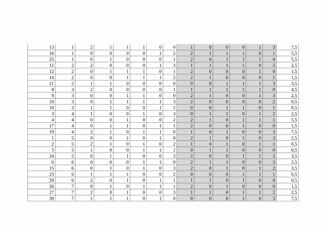
13 1 2 1 1 1 0 0 1 0 0 0 1 3 7,5
16 1 0 0 0 0 1 2 2 1 1 1 0 1 5,5
25 1 0 1 0 0 0 1 2 0 1 1 1 0 5,5
11 2 2 0 0 0 1 3 1 1 1 1 0 2 2,5
12 2 0 1 1 1 0 1 2 0 0 0 1 0 1,5
14 2 0 0 1 1 1 2 2 1 0 0 0 1 1,5
21 2 1 1 0 0 0 0 0 0 1 1 1 3 3,5
8 3 2 0 0 0 0 1 1 1 1 1 1 0 4,5
9 3 0 0 1 1 0 0 2 1 0 0 1 3 2,5
10 3 0 1 1 1 1 3 2 0 0 0 0 2 0,5
18 3 1 1 0 0 1 2 0 0 1 1 0 1 0,5
3 4 1 0 0 1 0 3 0 1 1 0 1 2 2,5
4 4 0 0 1 0 0 2 2 1 0 1 1 1 5,5
17 4 0 1 1 0 1 1 2 0 0 1 0 0 1,5
19 4 2 1 0 1 1 0 1 0 1 0 0 3 7,5
1 5 0 0 1 0 1 0 2 1 0 1 0 3 2,5
2 5 2 1 0 1 0 2 1 0 1 0 1 1 0,5
5 5 1 0 0 1 1 1 0 1 1 0 0 0 0,5
24 5 0 1 1 0 0 3 2 0 0 1 1 2 3,5
6 6 0 0 0 1 1 0 2 1 1 0 0 3 2,5
15 6 0 1 0 1 0 3 2 0 1 0 1 2 3,5
23 6 1 1 1 0 0 2 0 0 0 1 1 1 0,5
29 6 2 0 1 0 1 1 1 1 0 1 0 0 0,5
26 7 0 1 0 1 1 1 2 0 1 0 0 0 1,5
27 7 2 0 1 0 0 3 1 1 0 1 1 2 2,5
30 7 1 1 1 0 1 0 0 0 0 1 0 3 7,5

31 7 0 0 0 1 0 2 2 1 1 0 1 1 5,5

116
Appendix B: Survey Questionnaire
FIELD SURVEY FOR
MOBILE TELECOMMUNICATIONS USE AND DEMAND FOR SERVICE
IMPROVEMENTS IN TRNC
This survey is being conducted for use in an ongoing dissertation research project at
Eastern Mediterranean University Economics Department, on the topic of mobile
telecommunications use and demand for service improvements (such as 4G and cost-
free use when abroad) in TRNC.
Section 1: Mobile Phone and Internet Use
1. Which mobile telecommunications devices listed below do you possess? (Please
check all that apply)
a. Regular mobile phone [ ]
b. Smart phone (iPhone, Samsung Galaxy and likes) [ ]
c. Tablet (iPad and likes) [ ]
d. Laptop [ ]
2. Do you possess any personal GSM numbers/sim cards (registered in TRNC) which
you use in your mobile devices?
a. Yes I do [ ] ...................How many?: ______________ number(s)
b. No I don’t [ ]
If your response to Question 2 is “No I don’t”, please continue with Question 21.

117
3. How much do you pay monthly on average for your personal GSM number? If you
own more than one number, please write seperately the monthly amount you pay for
each of your GSM numbers. (Inclusive of mobile speaking, SMS, internet service costs
and taxes)
Please write: _______ TL per month (for my primary GSM number)
_______ TL per month (for my 2nd GSM number)
_______ TL per month (for my 3rd GSM number)
4. How frequently do you use the mobile internet service provided by your GSM
subscription?
a. Every day [ ]
b. Several times a week [ ]
c. Several times a month [ ]
d. Very rarely [ ]
e. Never [ ]
If your response to Question 4 is “Never”, please continue with Question 9.
5. For which purposes do you use the mobile internet service provided by your GSM
subscription? (Please check all that apply)
a. Search engines (e.g. Google) [ ]
b. E-mail [ ]
c. Instant messaging (e.g. WhatsApp) [ ]
d. Voice over IP (speaking on the internet) [ ]
e. Videophone (speaking on the internet with video) [ ]
f. Social networking sites (e.g. Facebook, Twitter, Instagram) [ ]

118
g. News sites [ ]
h. Watching videos [ ]
i. Watching movies [ ]
j. Other mobile applications (e.g. downloaded from App Store) [ ]
k. Cloud computing (i.e. storing personal documents over the net) [ ]
l. To connect my laptop/computer to the internet wirelessly [ ]
6. For how many hours per week on average do you use the mobile internet service
provided by your GSM subscription?
Please write: ______________ hours per week
7. How do you purchase the mobile internet service provided by your GSM
subscription?
a. Monthly flat-sum plan (I buy a mobile internet package with a data
limit) [ ]
b. Meter-rate billing plan (I pay as much as I use) [ ]
If your response to Question 7 is “Meter-rate billing plan”, please continue with
Question 9.
8. What is the data limit of the mobile internet package you have on your GSM
subscription?
Please write: ______________ MB/GB per month

119
9. Do you experience any problems with your GSM services such as
noise/disconnection when speaking, or slowing/freezing/not connecting with your
mobile internet?
a. Yes I do [ ]
b. No I don’t [ ]
If your response to Question 9 is “No I don’t”, please continue with Question 11.
10. How frequently do you face the problems mentioned in Question 9?
a. Every day [ ]
b. Once or several times a week [ ]
c. Once or several times a month [ ]
d. Once every few months [ ]
e. Never [ ]
11. Speaking or using mobile internet in Turkey with your TRNC GSM
number/subscription are subject to “roaming” costs. How frequently do you travel to
Turkey? Please write the average number of days which you are in Turkey in one year.
Please write: ______________ days on average, in one year
12. Suppose it was possible to speak and use mobile internet in Turkey with your
current TRNC GSM subcription, number and plan. Would you be interested?
a. Yes I would be interested [ ]
b. No I wouldn’t be interested [ ]

120
13. Speaking or using mobile internet in South Cyprus with your TRNC GSM
number/subscription is not possible due to the current political problem (except for
regions which are close to the Northern border and have signal coverage from
transmitters in the North). How frequently do you travel to South Cyprus? Please write
the average number of days which you are in South Cyprus in one year.
Please write: ______________ days on average, in one year
14. Suppose it was possible to speak and use mobile internet in South Cyprus with
your current North Cyprus GSM subscription, number and plan. Would you be
interested?
a. Yes I would be interested [ ]
b. No I wouldn’t be interested [ ]

121
Section 2: Willingness to Pay for 4G
Fourth generation mobile communications technology, known as 4G, is a new
technology which enables both high-quality voice conversation and very high speed
mobile internet connectivity. 4G mobile internet has a minimum connection speed of
30 Mbit/s, and it is capable of providing speeds up to 300 Mbit/s. The 3G technology
currently in use in TRNC provides an average speed of 3 Mbit/s. This means 4G
mobile internet is 10 to 100 times faster than 3G mobile internet.
“Very high speed” mobile internet connectivity provided by 4G technology will make
it possible to take advantage of the following:
Mobile “videophone” conversations can be made.
Videos and movies on the internet will display instantly.
Real-time games on the internet can be played while mobile.
No freezing/disconnection in the video/movie/game stream while on the move.
(e.g. travelling in a car)
Very large file transfers can be made instantly over the internet.
Cloud computing can be used while mobile. With the very high speed mobile
internet connectivity, all personal files can be stored on the internet and
displayed on all personal mobile devices.
Because 4G mobile internet service can be used for home internet connection
as well, you may opt not to purchase a seperate home internet service.
Another advantage of the 4G technology when compared with 3G, is that 4G is better
in quality, in other words 4G provides a higher quality voice conversation and
mobile internet connection capability. 4G users never experience any freezing or
disconnection while speaking on their mobile phone or surfing the internet.
In order for 4G technology to be available in TRNC, investments need to be made to
build the infrastructure. In order to elaborate on the investments to make, the returns

122
of the 4G for the people of TRNC should be established. This section aims to quantify
the monetary value of 4G for the consumer.
Note 1: Please respond to the question below, considering only your own needs and
your own budget.
Note 2: The purpose of this survey is only academic. It is not being administered by
the government or by any private firm for pricing 4G. Your responses will not affect
any possible 4G prices in the future.
15. Would you be willing to pay for a 4G service which provides mobile internet
speed 10 times faster than 3G, unlimited internet use, and no
freezing/disconnection in speaking or internet connectivity, if the additional cost
on your monthly GSM bill (per subscription) were...
Put a tick [ ]
next to the
HIGHEST amount
that you are sure
you would pay.
Put a cross [ ]
next to the FIRST
amount that you
are sure you would
not pay.
Additional cost on monthly GSM bill
1. Would not go for 4G. [ ]
2. 5 TL additional per month [ ]
3. 10 TL additional per month [ ]
4. 15 TL additional per month [ ]
5. 20 TL additional per month [ ]
6. 25 TL additional per month [ ]
7. 30 TL additional per month [ ]
8. 40 TL additional per month [ ]
9. 50 TL additional per month [ ]
10. 70 TL additional per month [ ]
11. 100 TL additional per month [ ]

123
12. 150 TL additional per month [ ]
13. 200 TL additional per month [ ]
14. 300 TL additional per month [ ]
15. More than 300 TL per month
Minimum WTP: _____TL per month
Maximum WTP: _____TL per month
[ ]
If your response to Question 17 is “Would not go for 4G”, please continue with
Question 18. If not, please continue with Section 3.
16. What are the reasons that you would not go for 4G?
Please write:
________________________________________________________
________________________________________________________
________________________________________________________
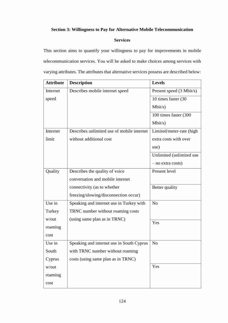
124
Section 3: Willingness to Pay for Alternative Mobile Telecommunication
Services
This section aims to quantify your willingness to pay for improvements in mobile
telecommunication services. You will be asked to make choices among services with
varying attributes. The attributes that alternative services possess are described below:
Attribute Description Levels
Internet
speed
Describes mobile internet speed Present speed (3 Mbit/s)
10 times faster (30
Mbit/s)
100 times faster (300
Mbit/s)
Internet
limit
Describes unlimited use of mobile internet
without additional cost
Limited/meter-rate (high
extra costs with over
use)
Unlimited (unlimited use
– no extra costs)
Quality Describes the quality of voice
conversation and mobile internet
connectivity (as to whether
freezing/slowing/disconnection occur)
Present level
Better quality
Use in
Turkey
w/out
roaming
cost
Speaking and internet use in Turkey with
TRNC number without roaming costs
(using same plan as in TRNC)
No
Yes
Use in
South
Cyprus
w/out
roaming
cost
Speaking and internet use in South Cyprus
with TRNC number without roaming
costs (using same plan as in TRNC)
No
Yes

125
Additional
monthly
cost
Additional monthly GSM cost per
subscription
20 TL
40 TL
60 TL
80 TL
Now you will be asked to make 4 service choices. You will be presented with 3
alternatives (A, B, C) in every choice question: 2 new mobile telecommunication
services (A, B) and 1 current service you are actually using now (C). The 2 new
services will have varying levels for the attributes listed above. Your current service,
to remind you, has the following attribute levels:
1. Current service internet speed: Present speed (The only mobile technology currently
available in TRNC is 3G)
2. Current service internet limit: Limited/meter-rate (Current GSM operators in TRNC
have no plans or packages which offer unlimited mobile internet use)
3. Current service internet quality: Present level
4. Use in Turkey w/out roaming cost with current service: No
5. Use in South Cyprus w/out roaming cost with current service: No
6. Additional monthly cost: 0 TL (No additional cost because it’s the current service)
Please make every choice as you would do if you faced a similar situation in real life.
If you prefer one of the new services please select that service, or if you prefer to stay
with your current service please select the current service.
(Note: In order to comprehend the amount of mobile internet offered by a
“limited/meter-rate” service, you may consider it will be similar to the “limited/meter-
rate” experience you have with your current service.)

126
17. Among 3 alternative mobile telecommunication services listed below (Service A,
Service B and Service C), please choose the one you prefer.
Service A Service B Service C (Current Service)
Internet speed 10 times faster Present speed Present speed
Internet limit Unlimited Limited/meter-
rate Limited/meter-
rate
Quality (voice and internet) Better quality Present level Present level
Use in Turkey w/out roaming cost
No Yes No
Use in S. Cyprus w/out roaming cost
No Yes No
Additional monthly cost 80 TL 60 TL 0 TL
Your choice: [ ] [ ] [ ]
18. Among 3 alternative mobile telecommunication services listed below (Service A,
Service B and Service C), please choose the one you prefer.
Service A Service B Service C (Current Service)
Internet speed Present speed 10 times faster Present speed
Internet limit Unlimited Limited/meter-
rate Limited/meter-
rate
Quality (voice and internet) Present level Better quality Present level
Use in Turkey w/out roaming cost
Yes No No
Use in S. Cyprus w/out roaming cost
Yes No No
Additional monthly cost 60 TL 40 TL 0 TL
Your choice: [ ] [ ] [ ]

127
19. Among 3 alternative mobile telecommunication services listed below (Service A,
Service B and Service C), please choose the one you prefer.
Service A Service B Service C (Current Service)
Internet speed Present speed 10 times faster Present speed
Internet limit Limited/meter-
rate Unlimited
Limited/meter-rate
Quality (voice and internet) Present level Better quality Present level
Use in Turkey w/out roaming cost
No Yes No
Use in S. Cyprus w/out roaming cost
No Yes No
Additional monthly cost 20 TL 80 TL 0 TL
Your choice: [ ] [ ] [ ]
20. Among 3 alternative mobile telecommunication services listed below (Service A,
Service B and Service C), please choose the one you prefer.
Service A Service B Service C (Current Service)
Internet speed 10 times faster Present speed Present speed
Internet limit Limited/meter-
rate Unlimited
Limited/meter-rate
Quality (voice and internet) Better quality Present level Present level
Use in Turkey w/out roaming cost
Yes No No
Use in S. Cyprus w/out roaming cost
Yes No No
Additional monthly cost 40 TL 20 TL 0 TL
Your choice: [ ] [ ] [ ]

128
Section 4: Demographic Questions
21. District: a. Girne [ ] b. G.yurt [ ] c. İskele [ ] d. Lefkoşa [ ] e. Mağusa [ ]
22. Your age: ______________ (please write)
23. Your gender: a. Female [ ] b. Male [ ]
24. Your marital status: a. Married [ ] b. Not married [ ]
25. Your education: a. Primary school [ ] b. Secondary school [ ] c. High school
/ Vocational [ ] d. University (2-year) [ ] e. University (4-
year) [ ] f. Graduate school (Master) [ ] g. Graduate school
(Doctorate) [ ]
26. Employment: a. Employed [ ] b. Unemployed [ ]
27. Your net monthly income (After-tax net income inclusive of your wage, family
contributions, state contributions, rents and returns on investment):
______________ TL per month
28. Nationality: a. Only TRNC [ ] b. Dual (TRNC and other) [ ]
c. Other [ ]
THE END
THANK YOU FOR YOUR VALUABLE TIME.

129
Section 5: Post Interview (For interviewer only)
Please rate the quality of the interview based on the concentration of the person to be
interviewed, attentiveness to the questions, and number of questions answered:
a. Very good [ ]
b. Good [ ]
c. Fair [ ]
d. Poor [ ]
e. Very poor [ ]
Name of the interviewer: ...................................................................
Date of interview: ...................................................................
Time started: ...................................................................
Duration of the interview: ...................................................................