1

Estimating Zonal Electricity Supply Curves in

Transmission-Constrained Electricity Markets

Mostafa Sahraei-Ardakani*, Seth Blumsack**, Andrew Kleit**

*School of Electrical, Computer, and Energy Engineering, Arizona State University

**John and Willie Leone Family Department of Energy and Mineral Engineering,

The Pennsylvania State University

Corresponding author: Seth Blumsack, Department of Energy and Mineral Engineering, 124

Hosler Building, University Park PA, 16802. Tel: +1 (814) 863-7597. E-mail: sab51@psu.edu

Keywords: carbon tax; demand response policy; electricity markets; Pennsylvania’s act 129;

transmission constraints; zonal electricity supply curve

Abstract

Many important electricity policy initiatives would directly affect the operation of electric

power networks. This paper develops a method for estimating short-run zonal supply curves in

transmission-constrained electricity markets that can be implemented quickly by policy analysts

with training in statistical methods and with publicly available data. Our model enables analysis

of distributional impacts of policies affecting operation of electric power grid. The method uses

fuel prices and zonal electric loads to determine piecewise supply curves, identifying zonal elec-

tricity price and marginal fuel. We illustrate our methodology by estimating zonal impacts of

Pennsylvania’s act 129, an energy efficiency and conservation policy. For most utilities in Penn-

sylvania, act 129 would reduce the influence of natural gas on electricity price formation and in-

crease the influence of coal. The total resulted savings would be around 267 million dollars, 82

percent of which would be enjoyed by the customers in Pennsylvania. We also analyze the im-

pacts of imposing a $35/ton tax on carbon dioxide emissions. Our results show that the policy

would increase the average prices in PJM by 47 to 89 percent under different fuel price scenarios

in the short run, and would lead to short-run interfuel substitution between natural gas and coal.

1. Introduction

Many energy and environmental policy initiatives (including emissions regulations; renewa-

ble portfolio standards; and efficiency policies) would affect the operation of electric power grid.

2

Analysis of such policies is however difficult in the absence of reliable models of the electric

power system. The North American power transmission grid has been called “the largest and

most complex machine in the world” [1]. Detailed modeling of the system requires complete en-

gineering data on every element of the system such as transmission lines, transformers and gen-

erators. This engineering approach is often not feasible in the context of policy analysis due to

the proprietary nature of the data and engineering model complexity. Moreover, policy analysis

involves the study of future scenarios. Thus, the inputs to the model should be estimated for the

future, which always involves some degree of uncertainty. Since the engineering models need

detailed data, the set of input uncertainties becomes extremely large. There exist, many other

methods in the literature for forecasting short term electricity prices, including probabilistic es-

timation of price duration curves [2], short term forecast with fuzzy neural networks [3-4], trans-

fer functions [5], and linear and nonlinear time series[6-9]. These methods are designed to fore-

cast short term prices from hours to a week ahead. They estimate short-term prices well but can-

not be used in policy analysis, where acceptable performance over longer periods of time is

needed. Abstract equilibrium models such as [10] can provide insights into strategic gaming and

market design efficiency, but cannot be directly applied to real markets.

As a result, many policy models in the existing literature neglect the effects of the transmis-

sion system and use the relatively simple dispatch curve models [11-19]. In order to construct a

dispatch curve, power plants in a system are sorted according to their marginal cost. The data

needed for calculating marginal cost includes heat rate, fuel type and capacity, which are publi-

cally available through e-GRID [20] or other similar data sources. Fig. 1 shows an estimated

dispatch curve for Pennsylvania-New Jersey-Maryland interconnection (PJM) and is calculated

similar to [13]. PJM currently serves all or parts of Delaware, Illinois, Indiana, Kentucky, Mary-

3

land, Michigan, New Jersey, North Carolina, Ohio, Pennsylvania, Tennessee, Virginia, West

Virginia and the District of Columbia. Given data on electricity demand, the dispatch curve can

be utilized to determine the marginal unit in the system, as well as the market price in the ab-

sence of transmission constraints (the so-called “System Marginal Price”). However, because of

the transmission constraints, both prices and marginal technologies can be potentially different at

different locations within the power system. For example in PJM during the peak hours prices

are much higher in eastern areas such as Philadelphia and Washington, D.C. than Western Penn-

sylvania and West Virginia. At such times, coal may be on the margin in the western PJM while

oil is on the margin in eastern PJM.

Locational price differences induced by transmission congestion can introduce challenges in

the context of policy analysis. We take as an example Pennsylvania’s Act 129, which is an ener-

gy conservation and efficiency policy that requires the state’s utilities to reduce their annual de-

mand by one percent with 4.5% additional peak demand shaving.1 By looking at the dispatch

curve in Fig. 1, one can see that the slope of the supply curve is low when the demand is less

than 250 GWh, and a policy analyst assessing the price impact of Act 129 would predict that the

Act would not materially reduce wholesale prices in the PJM system (and, consequently, in

Pennsylvania). Such an assessment would ignore important locational price differences, with

two potential consequences. First, the estimated potential impacts of an efficiency policy such as

Act 129 are likely to be biased downwards, since they would not capture the steeper supply

curves (higher-cost generation) used in locations downstream from transmission constraints.

Second, the policy analyst would not be able to estimate locational differences in price impacts

and fuels utilization. These locational impacts may be important outcomes of the policy.

1 The full text of Act 129 can be found online at

http://www.puc.state.pa.us/electric/pdf/Act129/HB2200-Act129_Bill.pdf

4

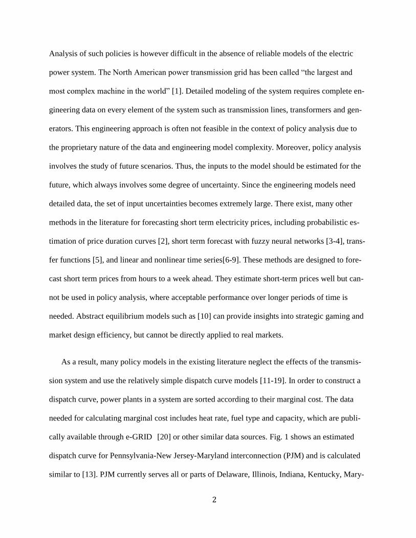
Fig. 1 suggests that, for a year similar to 2008, we can differentiate the technologies in the

supply curve and find thresholds based on demand levels, where the marginal input fuel switch-

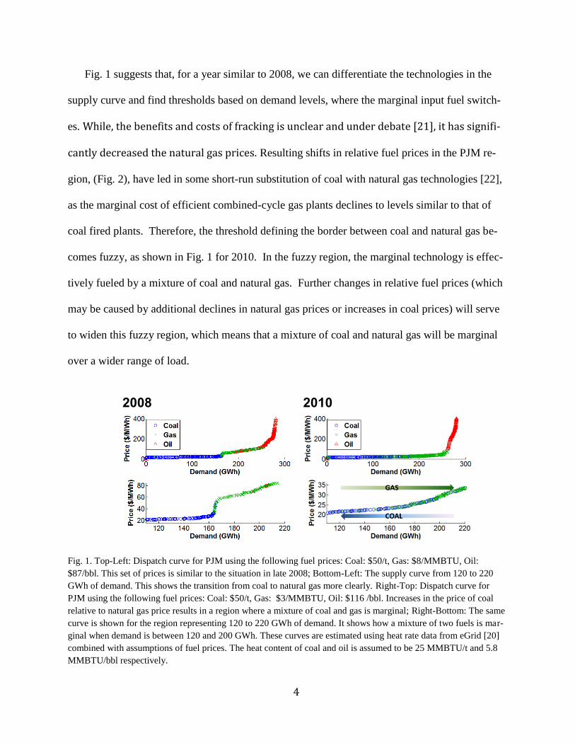
es. While, the benefits and costs of fracking is unclear and under debate [21], it has signifi-

cantly decreased the natural gas prices. Resulting shifts in relative fuel prices in the PJM re-

gion, (Fig. 2), have led in some short-run substitution of coal with natural gas technologies [22],

as the marginal cost of efficient combined-cycle gas plants declines to levels similar to that of

coal fired plants. Therefore, the threshold defining the border between coal and natural gas be-

comes fuzzy, as shown in Fig. 1 for 2010. In the fuzzy region, the marginal technology is effec-

tively fueled by a mixture of coal and natural gas. Further changes in relative fuel prices (which

may be caused by additional declines in natural gas prices or increases in coal prices) will serve

to widen this fuzzy region, which means that a mixture of coal and natural gas will be marginal

over a wider range of load.

Fig. 1. Top-Left: Dispatch curve for PJM using the following fuel prices: Coal: $50/t, Gas: $8/MMBTU, Oil:

$87/bbl. This set of prices is similar to the situation in late 2008; Bottom-Left: The supply curve from 120 to 220

GWh of demand. This shows the transition from coal to natural gas more clearly. Right-Top: Dispatch curve for

PJM using the following fuel prices: Coal: $50/t, Gas: $3/MMBTU, Oil: $116 /bbl. Increases in the price of coal

relative to natural gas price results in a region where a mixture of coal and gas is marginal; Right-Bottom: The same

curve is shown for the region representing 120 to 220 GWh of demand. It shows how a mixture of two fuels is mar-

ginal when demand is between 120 and 200 GWh. These curves are estimated using heat rate data from eGrid [20]

combined with assumptions of fuel prices. The heat content of coal and oil is assumed to be 25 MMBTU/t and 5.8

MMBTU/bbl respectively.

2008 2010

5

Here we seek to develop a model with publicly available data that can capture locational dif-

ferences in technologies and fuels that are on the margin in transmission-constrained electricity

systems. Our method implicitly models transmission constraints by estimating electricity price

and marginal fuel at the zonal level as a function of zonal and system-level electricity demand.

(Large-scale power systems are often divided into geographic “zones” for planning, pricing or

other purposes; see [23]). The rest of this paper is organized as follows: A simple example

which motivates our method is presented in section 2. Our econometric model is described in

section 3. Section 4 presents the application of our method to seventeen utility zone of PJM as

well as the simulation of Pennsylvania Act 129 and a carbon tax policy. Section 5 concludes the

paper.

Fig. 2. Fuel price trends since January 2006.

2. Motivating Example

The following example shows how transmission constraints introduce complexities in build-

ing supply curves and performing policy analysis. Fig. 3 shows a simple electric system with

two nodes. There is a single generator and single customer or “load” at each node. The genera-

tors are assumed to have simple linear marginal cost functions; MC(G1) = 5 + G1 for the genera-

0

5

10

15

20

25

Jan

-06

Ap

r-0

6

Jul-

06

Oct

-06

Jan

-07

Ap

r-0

7

Jul-

07

Oct

-07

Jan

-08

Ap

r-0

8

Jul-

08

Oct

-08

Jan

-09

Ap

r-0

9

Jul-

09

Oct

-09

Jan

-10

Ap

r-1

0

Jul-

10

Oct

-10

$/M

MB

TU

OIL

GAS

COAL

6

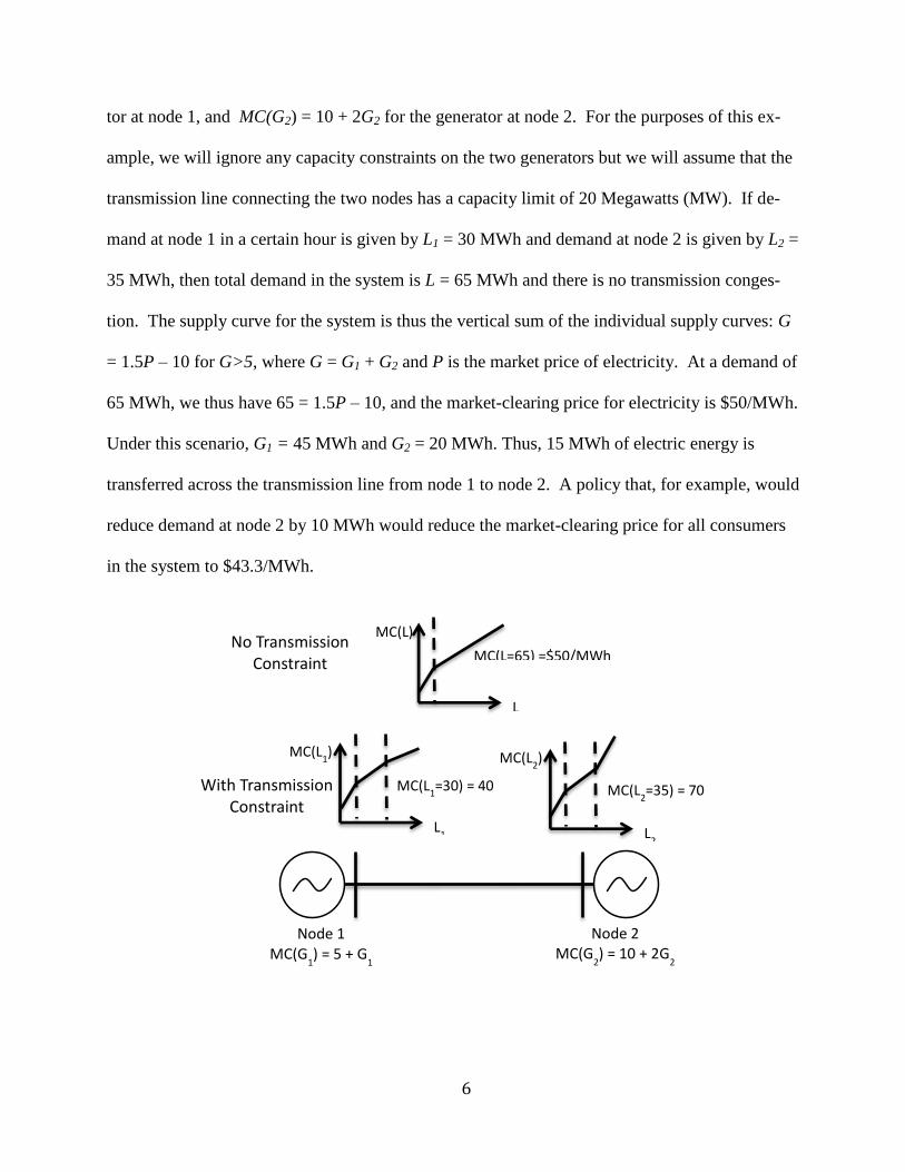
tor at node 1, and MC(G2) = 10 + 2G2 for the generator at node 2. For the purposes of this ex-

ample, we will ignore any capacity constraints on the two generators but we will assume that the

transmission line connecting the two nodes has a capacity limit of 20 Megawatts (MW). If de-

mand at node 1 in a certain hour is given by L1 = 30 MWh and demand at node 2 is given by L2 =

35 MWh, then total demand in the system is L = 65 MWh and there is no transmission conges-

tion. The supply curve for the system is thus the vertical sum of the individual supply curves: G

= 1.5P – 10 for G>5, where G = G1 + G2 and P is the market price of electricity. At a demand of

65 MWh, we thus have 65 = 1.5P – 10, and the market-clearing price for electricity is $50/MWh.

Under this scenario, G1 = 45 MWh and G2 = 20 MWh. Thus, 15 MWh of electric energy is

transferred across the transmission line from node 1 to node 2. A policy that, for example, would

reduce demand at node 2 by 10 MWh would reduce the market-clearing price for all consumers

in the system to $43.3/MWh.

Node 1

MC(G1) = 5 + G

1

Node 2 MC(G

2) = 10 + 2G

2

L1

MC(L1)

L2

MC(L2)

L

MC(L) No Transmission

Constraint

With Transmission Constraint

MC(L=65) =$50/MWh

MC(L1=30) = 40 MC(L

2=35) = 70

7

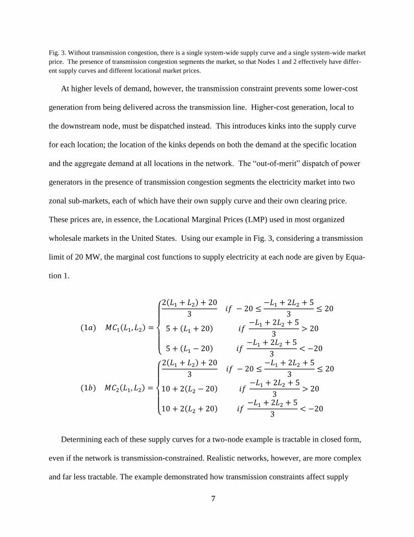
Fig. 3. Without transmission congestion, there is a single system-wide supply curve and a single system-wide market

price. The presence of transmission congestion segments the market, so that Nodes 1 and 2 effectively have differ-

ent supply curves and different locational market prices.

At higher levels of demand, however, the transmission constraint prevents some lower-cost

generation from being delivered across the transmission line. Higher-cost generation, local to

the downstream node, must be dispatched instead. This introduces kinks into the supply curve

for each location; the location of the kinks depends on both the demand at the specific location

and the aggregate demand at all locations in the network. The “out-of-merit” dispatch of power

generators in the presence of transmission congestion segments the electricity market into two

zonal sub-markets, each of which have their own supply curve and their own clearing price.

These prices are, in essence, the Locational Marginal Prices (LMP) used in most organized

wholesale markets in the United States. Using our example in Fig. 3, considering a transmission

limit of 20 MW, the marginal cost functions to supply electricity at each node are given by Equa-

tion 1.

(1𝑎) 𝑀𝐶1(𝐿1, 𝐿2) =

{

2(𝐿1 + 𝐿2) + 20

3𝑖𝑓 − 20 ≤

−𝐿1 + 2𝐿2 + 5

3≤ 20

5 + (𝐿1 + 20) 𝑖𝑓 −𝐿1 + 2𝐿2 + 5

3> 20

5 + (𝐿1 − 20) 𝑖𝑓 −𝐿1 + 2𝐿2 + 5

3< −20

(1𝑏) 𝑀𝐶2(𝐿1, 𝐿2) =

{

2(𝐿1 + 𝐿2) + 20

3𝑖𝑓 − 20 ≤

−𝐿1 + 2𝐿2 + 5

3≤ 20

10 + 2(𝐿2 − 20) 𝑖𝑓 −𝐿1 + 2𝐿2 + 5

3> 20

10 + 2(𝐿2 + 20) 𝑖𝑓 −𝐿1 + 2𝐿2 + 5

3< −20

Determining each of these supply curves for a two-node example is tractable in closed form,

even if the network is transmission-constrained. Realistic networks, however, are more complex

and far less tractable. The example demonstrated how transmission constraints affect supply

8

curves at different locations of the system. It should be noted that, transmission constraints are

much more complicated in realistic meshed networks and we do not use this simplistic limit in

the rest of the paper.

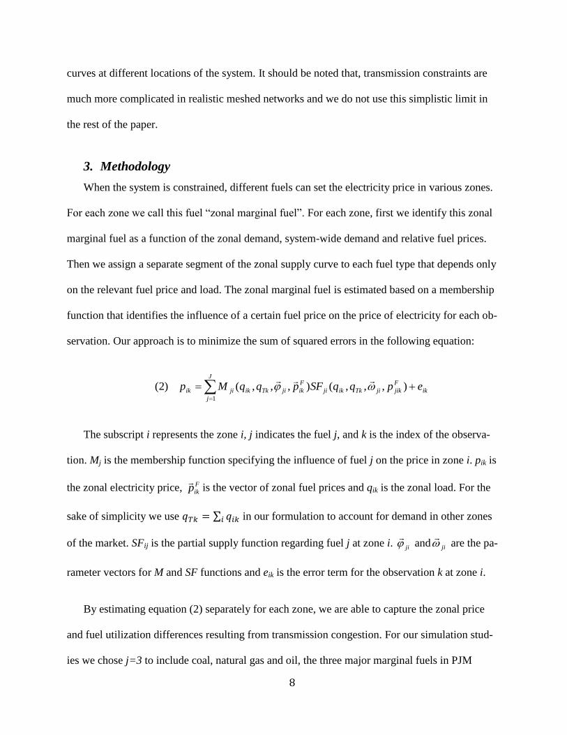
3. Methodology

When the system is constrained, different fuels can set the electricity price in various zones.

For each zone we call this fuel “zonal marginal fuel”. For each zone, first we identify this zonal

marginal fuel as a function of the zonal demand, system-wide demand and relative fuel prices.

Then we assign a separate segment of the zonal supply curve to each fuel type that depends only

on the relevant fuel price and load. The zonal marginal fuel is estimated based on a membership

function that identifies the influence of a certain fuel price on the price of electricity for each ob-

servation. Our approach is to minimize the sum of squared errors in the following equation:

J

j

ik

F

jikjiTkikji

F

ikjiTkikjiik epqqSFpqqMp1

),,,(),,,()2(

The subscript i represents the zone i, j indicates the fuel j, and k is the index of the observa-

tion. Mj is the membership function specifying the influence of fuel j on the price in zone i. pik is

the zonal electricity price, F

ikp

is the vector of zonal fuel prices and qik is the zonal load. For the

sake of simplicity we use 𝑞𝑇𝑘 = ∑ 𝑞𝑖𝑘𝑖 in our formulation to account for demand in other zones

of the market. SFij is the partial supply function regarding fuel j at zone i. ji

and ji

are the pa-

rameter vectors for M and SF functions and eik is the error term for the observation k at zone i.

By estimating equation (2) separately for each zone, we are able to capture the zonal price

and fuel utilization differences resulting from transmission congestion. For our simulation stud-

ies we chose j=3 to include coal, natural gas and oil, the three major marginal fuels in PJM

9

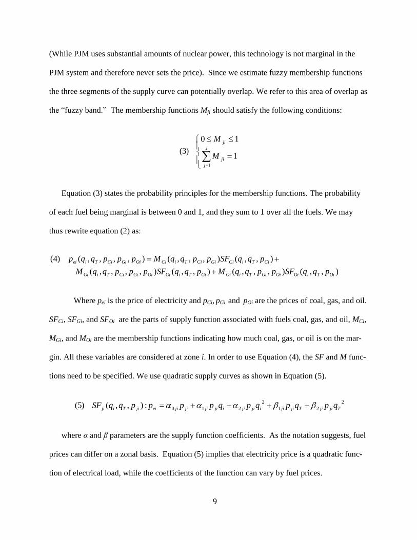
(While PJM uses substantial amounts of nuclear power, this technology is not marginal in the

PJM system and therefore never sets the price). Since we estimate fuzzy membership functions

the three segments of the supply curve can potentially overlap. We refer to this area of overlap as

the “fuzzy band.” The membership functions Mji should satisfy the following conditions:

J

j

ji

ji

M

M

1

1

10

)3(

Equation (3) states the probability principles for the membership functions. The probability

of each fuel being marginal is between 0 and 1, and they sum to 1 over all the fuels. We may

thus rewrite equation (2) as:

),,(),,,(),,(),,,,(

),,(),,,(),,,,()4(

OiTiOiOiGiTiOiGiTiGiOiGiCiTiGi

CiTiCiGiCiTiCiOiGiCiTiei

pqqSFppqqMpqqSFpppqqM

pqqSFppqqMpppqqp

Where pei is the price of electricity and pCi, pGi and pOi are the prices of coal, gas, and oil.

SFCi, SFGi, and SFOi are the parts of supply function associated with fuels coal, gas, and oil, MCi,

MGi, and MOi are the membership functions indicating how much coal, gas, or oil is on the mar-

gin. All these variables are considered at zone i. In order to use Equation (4), the SF and M func-

tions need to be specified. We use quadratic supply curves as shown in Equation (5).

2

21

2

210:),,()5( TjijiTjijiijijiijijijijieijiTiji qpqpqpqppppqqSF

where α and β parameters are the supply function coefficients. As the notation suggests, fuel

prices can differ on a zonal basis. Equation (5) implies that electricity price is a quadratic func-

tion of electrical load, while the coefficients of the function can vary by fuel prices.

10

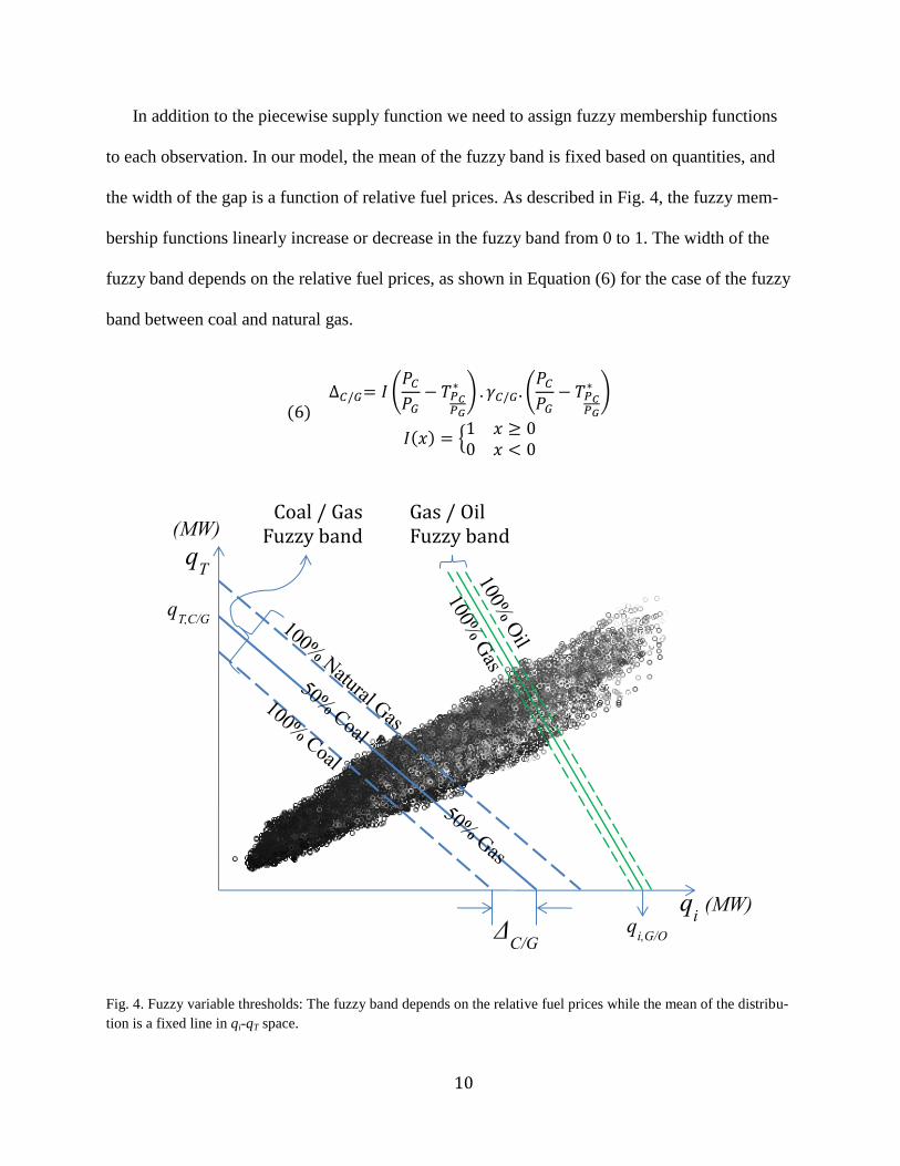
In addition to the piecewise supply function we need to assign fuzzy membership functions

to each observation. In our model, the mean of the fuzzy band is fixed based on quantities, and

the width of the gap is a function of relative fuel prices. As described in Fig. 4, the fuzzy mem-

bership functions linearly increase or decrease in the fuzzy band from 0 to 1. The width of the

fuzzy band depends on the relative fuel prices, as shown in Equation (6) for the case of the fuzzy

band between coal and natural gas.

(6)∆𝐶/𝐺= 𝐼 (

𝑃𝐶𝑃𝐺− 𝑇𝑃𝐶

𝑃𝐺

∗ ) . 𝛾𝐶/𝐺 . (𝑃𝐶𝑃𝐺− 𝑇𝑃𝐶

𝑃𝐺

∗ )

𝐼(𝑥) = {1 𝑥 ≥ 00 𝑥 < 0

Fig. 4. Fuzzy variable thresholds: The fuzzy band depends on the relative fuel prices while the mean of the distribu-

tion is a fixed line in qi-qT space.

qi (MW)

(MW)

qT

ΔC/G

Gas / Oil Fuzzy band

qT,C/G

qi,G/O

Coal / Gas Fuzzy band

11

In Equation (6), PC is the price of coal, PG is the price of natural gas and 𝑇𝑃𝐶𝑃𝐺

∗ is the mini-

mum relative price (i.e., the price of coal relative to the price of gas) needed for the existence of

a fuzzy band. For relative prices below this limit, our probabilistic model becomes similar to the

model described and used in [24-26], where the thresholds separating segments of the supply

curve are defined by deterministic lines. The term 𝛾𝐶/𝐺 specifies how the fuzzy band widens

when the relative prices increase. We can write the same equation for the transition from gas to

oil as shown in Equation 7.

(7) ∆𝐺/𝑂= 𝐼 (𝑃𝐺𝑃𝑂− 𝑇𝑃𝐺

𝑃𝑂

∗ ) . 𝛾𝐺/𝑂 . (𝑃𝐺𝑃𝑂− 𝑇𝑃𝐺

𝑃𝑂

∗ )

Thus to fully identify the fuzzy thresholds we need to find qi,C/G , qi,G/O, qT,C/G , qT,G/O, 𝑇𝑃𝐶𝑃𝐺

∗ ,

𝛾𝐶/𝐺 ,𝑇𝑃𝐺𝑃𝑂

∗ and 𝛾𝐺/𝑂. Once these parameters are specified we can use an ordinary least squared

(OLS) regression method to estimate the parameters in Equation (5). To minimize the sum of

squared errors in Equation (2), we need to find the optimal parameters for the fuzzy threshold.

Estimation of the membership functions’ parameters is an optimization problem with the objec-

tive of minimizing the sum of squared errors. With different threshold parameters, the set of ob-

servations belonging to a specific fuel would change. However, marginal perturbation of the

threshold parameters would likely not change such sets. Thus, the objective function has a step-

wise shape, with billions of steps and flat regions, making it non-linear, non-differentiable, and

non-convex. Moreover, our examinations show that the objective function is multi-modal with

multiple local minima. Therefore, classical optimization algorithms fail to handle the problem.

We use a powerful evolutionary optimization algorithm known as Covariance Matrix Adapta-

tion-Evolution Strategy (CMA-ES). It takes samples from the decision space and approximates

12

the covariance matrix from the fitness of the samples. In the first step of the algorithm, a number

of individual solutions (sets of parameter estimates) are generated. In each generation, OLS is

used to estimate the ω parameters (see Equation 2) for each individual solution. Then the sum of

squared errors is calculated and fed back to CMA-ES as the fitness of each solution. The fitness

values are used to rank individuals and generate the next generation of parameters for the mem-

bership functions. This process is repeated until the stopping criteria are met [27-28].

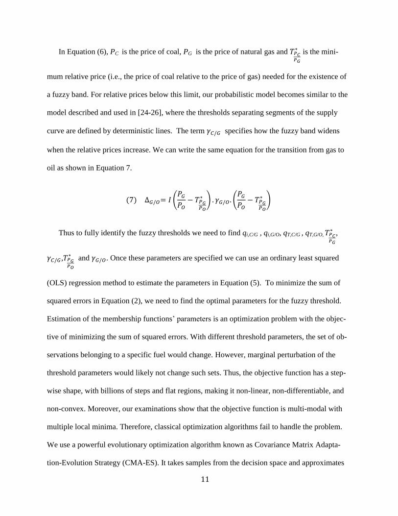
Fig. 5. Fuzzy membership function assignment for coal using analytical geometry formulation for linear plane.

After specifying all eight parameters needed for the fuzzy thresholds we use them to assign

membership functions to the data points. While the width of the fuzzy band depends on relative

fuel prices (and thus may vary from observation to observation), we assume that the mean of the

fuzzy band (the solid lines in Fig. 4) is fixed based on own area and PJM loads. Fig. 5 shows

qT,C/G

qi,C/G

qi,C/G

-ΔC/G

qi,C/G

+ΔC/G

qT,C/G

+m.ΔC/G

qT,C/G

-m.ΔC/G

m=qT,C/G

/ q

i,C/G

A

D

B

C

qi (MW)

qT (MW)

13

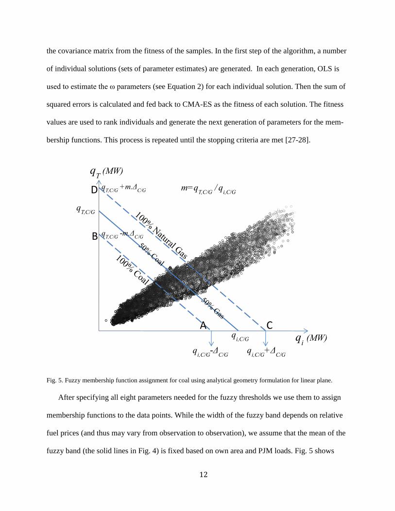
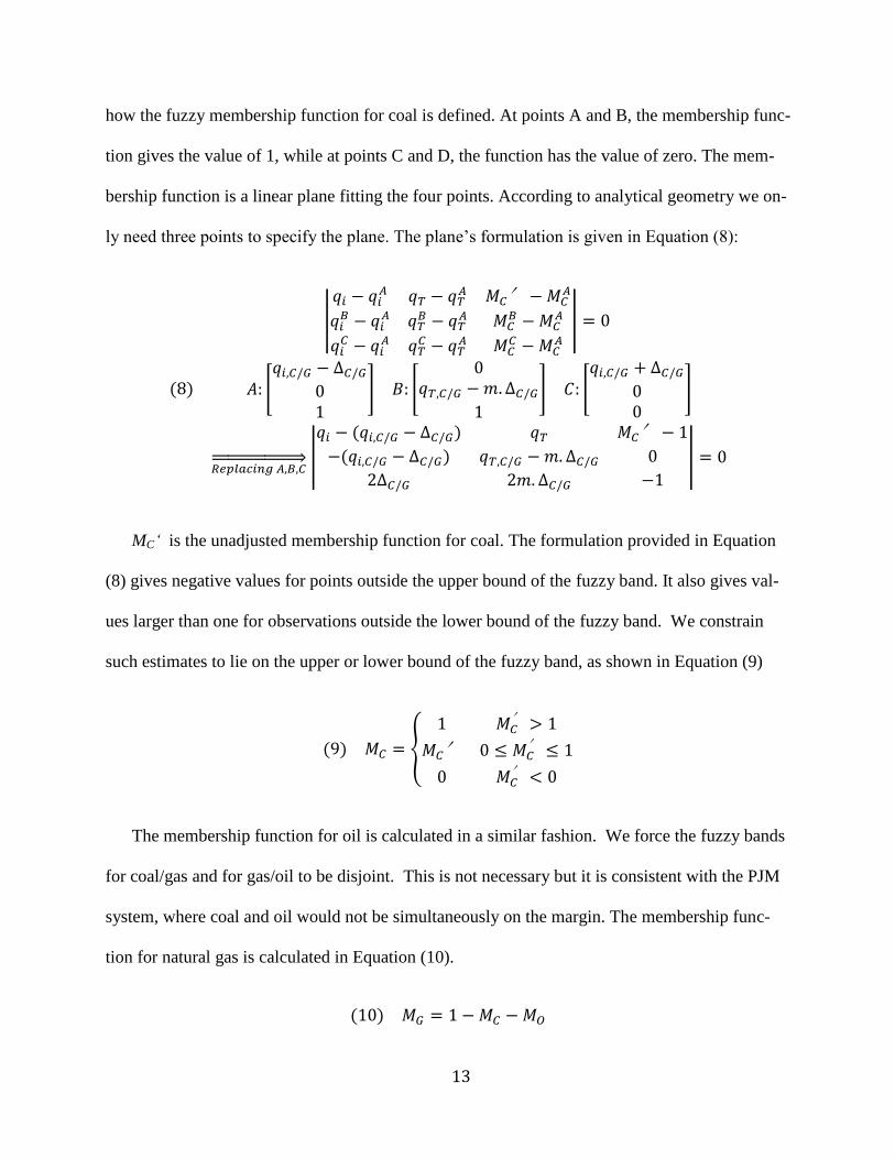
how the fuzzy membership function for coal is defined. At points A and B, the membership func-

tion gives the value of 1, while at points C and D, the function has the value of zero. The mem-

bership function is a linear plane fitting the four points. According to analytical geometry we on-

ly need three points to specify the plane. The plane’s formulation is given in Equation (8):

(8)

|

𝑞𝑖 − 𝑞𝑖𝐴 𝑞𝑇 − 𝑞𝑇

𝐴 𝑀𝐶′−𝑀𝐶𝐴

𝑞𝑖𝐵 − 𝑞𝑖

𝐴 𝑞𝑇𝐵 − 𝑞𝑇

𝐴 𝑀𝐶𝐵 −𝑀𝐶

𝐴

𝑞𝑖𝐶 − 𝑞𝑖

𝐴 𝑞𝑇𝐶 − 𝑞𝑇

𝐴 𝑀𝐶𝐶 −𝑀𝐶

𝐴

| = 0

𝐴: [𝑞𝑖,𝐶/𝐺 − ∆𝐶/𝐺

01

] 𝐵: [0

𝑞𝑇,𝐶/𝐺 −𝑚. ∆𝐶/𝐺1

] 𝐶: [𝑞𝑖,𝐶/𝐺 + ∆𝐶/𝐺

00

]

𝑅𝑒𝑝𝑙𝑎𝑐𝑖𝑛𝑔 𝐴,𝐵,𝐶⇒ |

𝑞𝑖 − (𝑞𝑖,𝐶/𝐺 − ∆𝐶/𝐺) 𝑞𝑇 𝑀𝐶′− 1

−(𝑞𝑖,𝐶/𝐺 − ∆𝐶/𝐺) 𝑞𝑇,𝐶/𝐺 −𝑚. ∆𝐶/𝐺 0

2∆𝐶/𝐺 2𝑚. ∆𝐶/𝐺 −1

| = 0

MC‘ is the unadjusted membership function for coal. The formulation provided in Equation

(8) gives negative values for points outside the upper bound of the fuzzy band. It also gives val-

ues larger than one for observations outside the lower bound of the fuzzy band. We constrain

such estimates to lie on the upper or lower bound of the fuzzy band, as shown in Equation (9)

(9) 𝑀𝐶 = {

1 𝑀𝐶′ > 1

𝑀𝐶′ 0 ≤ 𝑀𝐶′ ≤ 1

0 𝑀𝐶′ < 0

The membership function for oil is calculated in a similar fashion. We force the fuzzy bands

for coal/gas and for gas/oil to be disjoint. This is not necessary but it is consistent with the PJM

system, where coal and oil would not be simultaneously on the margin. The membership func-

tion for natural gas is calculated in Equation (10).

(10) 𝑀𝐺 = 1 −𝑀𝐶 −𝑀𝑂

14

Implementation of our method also requires adjustment of the price when estimating zonal

electricity prices within the fuzzy band. This is due to the fact that summation of coal and gas

parts of the supply curve, in the fuzzy region, would result in a higher price than the price influ-

enced by the mixture of the two fuels. We address this issue by adjusting zonal and system loads

within the fuzzy band to bound electricity price estimates from above. Our mechanism for

bounding price estimates in this way is described in detail in Appendix A.

4. Simulation Studies

We used zonal load and real time electricity prices obtained from the PJM website. We also

gathered state level fuel prices for electricity industry from the U.S. Energy Information Admin-

istration. Our data is from January 2006 to December 2010. The method explained in previous

section is utilized to estimate supply curves for each of the seventeen utility zones of PJM2. A

map of PJM is depicted in Fig. 6. The utility names with their abbreviations are presented in Ta-

ble 1.

Fig. 6. Geographical distribution of utilities in PJM electricity market

Table 1

PJM utility names and abbreviation

Utility Name Abbr. Utility Name Abbr.

2 Estimated Membership function and regression parameters, are available within the request from the

authors.

15

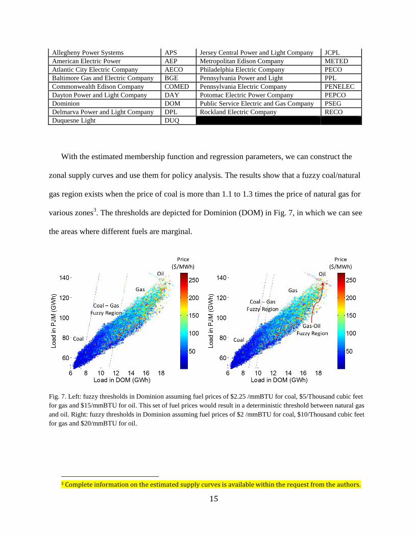
Allegheny Power Systems APS Jersey Central Power and Light Company JCPL

American Electric Power AEP Metropolitan Edison Company METED

Atlantic City Electric Company AECO Philadelphia Electric Company PECO

Baltimore Gas and Electric Company BGE Pennsylvania Power and Light PPL

Commonwealth Edison Company COMED Pennsylvania Electric Company PENELEC

Dayton Power and Light Company DAY Potomac Electric Power Company PEPCO

Dominion DOM Public Service Electric and Gas Company PSEG

Delmarva Power and Light Company DPL Rockland Electric Company RECO

Duquesne Light DUQ

With the estimated membership function and regression parameters, we can construct the

zonal supply curves and use them for policy analysis. The results show that a fuzzy coal/natural

gas region exists when the price of coal is more than 1.1 to 1.3 times the price of natural gas for

various zones3. The thresholds are depicted for Dominion (DOM) in Fig. 7, in which we can see

the areas where different fuels are marginal.

Fig. 7. Left: fuzzy thresholds in Dominion assuming fuel prices of $2.25 /mmBTU for coal, $5/Thousand cubic feet

for gas and $15/mmBTU for oil. This set of fuel prices would result in a deterministic threshold between natural gas

and oil. Right: fuzzy thresholds in Dominion assuming fuel prices of $2 /mmBTU for coal, $10/Thousand cubic feet

for gas and $20/mmBTU for oil.

3 Complete information on the estimated supply curves is available within the request from the authors.

16

We use our zonal supply curve to simulate the impacts of two policies in PJM. We first simu-

late the effects of imposing a carbon tax on electric generation. Then we study the impacts of

Pennsylvania Act 129 on utility zones in Pennsylvania and other PJM states.

4.1. Carbon Tax

The representative emissions of CO2 produced from each fuel per billion BTU of energy are

as follows: 94.35 tons for coal; 53.07 tons for natural gas; and 74.39 tons for oil. Each thousand

cubic feet of natural gas contains 1.03 MMBTU of energy. With the data on carbon emission by

fuel, we can calculate the equivalent fuel prices considering the carbon tax.

𝑃𝐶𝑜𝑎𝑙𝑇𝑎𝑥 = 𝑃𝐶𝑜𝑎𝑙 + 0.094 × 𝑇𝑎𝑥𝐶𝑎𝑟𝑏𝑜𝑛 (

$

𝑚𝑚𝐵𝑇𝑈)

𝑃𝐺𝑎𝑠𝑇𝑎𝑥 = 𝑃𝐺𝑎𝑠 + 0.054 × 𝑇𝑎𝑥𝐶𝑎𝑟𝑏𝑜𝑛 (

$

𝑇ℎ𝑜𝑢𝑠𝑎𝑛𝑑 𝑞𝑢𝑏𝑖𝑐 𝑓𝑒𝑒𝑡)

𝑃𝑂𝑖𝑙𝑇𝑎𝑥 = 𝑃𝑂𝑖𝑙 + 0.074 × 𝑇𝑎𝑥𝐶𝑎𝑟𝑏𝑜𝑛 (

$

𝑚𝑚𝐵𝑇𝑈)

PTax

represents the fuel price including the carbon tax. TaxCarbon has the unit of $/Ton of CO2.

British Columbia has implemented a carbon tax of $30/ton and comparable taxes are proposed

for Washington State [29]. Here, we study the impacts of imposing a carbon tax in the similar

range as in BC, $35 per ton of CO2, under two fuel price scenarios: a high natural gas price sce-

nario similar to [13] and a low natural gas price similar to fall 2010. For both scenarios we as-

sume price elasticity of demand to be -0.1 [30]. The fuel prices under each scenario are presented

in table 2.

Table 2

Fuel prices under the two scenarios

High gas price scenario [13] Low gas price scenario (Fall 2010)

Coal ($/MMBTU) 1.73 2.25

Natural Gas ($/MMBTU) 9.95 4

Oil ($/MMBTU) 8.49 15

17

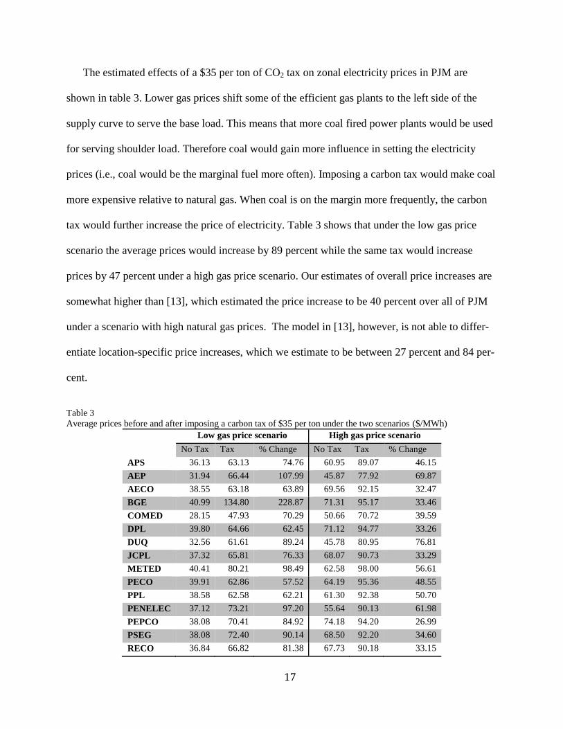
The estimated effects of a $35 per ton of CO2 tax on zonal electricity prices in PJM are

shown in table 3. Lower gas prices shift some of the efficient gas plants to the left side of the

supply curve to serve the base load. This means that more coal fired power plants would be used

for serving shoulder load. Therefore coal would gain more influence in setting the electricity

prices (i.e., coal would be the marginal fuel more often). Imposing a carbon tax would make coal

more expensive relative to natural gas. When coal is on the margin more frequently, the carbon

tax would further increase the price of electricity. Table 3 shows that under the low gas price

scenario the average prices would increase by 89 percent while the same tax would increase

prices by 47 percent under a high gas price scenario. Our estimates of overall price increases are

somewhat higher than [13], which estimated the price increase to be 40 percent over all of PJM

under a scenario with high natural gas prices. The model in [13], however, is not able to differ-

entiate location-specific price increases, which we estimate to be between 27 percent and 84 per-

cent.

Table 3

Average prices before and after imposing a carbon tax of $35 per ton under the two scenarios ($/MWh)

Low gas price scenario High gas price scenario

No Tax Tax % Change No Tax Tax % Change

APS 36.13 63.13 74.76 60.95 89.07 46.15

AEP 31.94 66.44 107.99 45.87 77.92 69.87

AECO 38.55 63.18 63.89 69.56 92.15 32.47

BGE 40.99 134.80 228.87 71.31 95.17 33.46

COMED 28.15 47.93 70.29 50.66 70.72 39.59

DPL 39.80 64.66 62.45 71.12 94.77 33.26

DUQ 32.56 61.61 89.24 45.78 80.95 76.81

JCPL 37.32 65.81 76.33 68.07 90.73 33.29

METED 40.41 80.21 98.49 62.58 98.00 56.61

PECO 39.91 62.86 57.52 64.19 95.36 48.55

PPL 38.58 62.58 62.21 61.30 92.38 50.70

PENELEC 37.12 73.21 97.20 55.64 90.13 61.98

PEPCO 38.08 70.41 84.92 74.18 94.20 26.99

PSEG 38.08 72.40 90.14 68.50 92.20 34.60

RECO 36.84 66.82 81.38 67.73 90.18 33.15

18

DAY 32.74 91.92 180.75 42.43 78.23 84.39

DOM 37.78 60.26 59.52 74.42 97.21 30.63

PJM 35.32 67.05 89.52 59.89 86.63 47.15

The carbon tax policy would also change fuels utilization. Table 4 presents our estimates of

how often each fuel is on the margin in each zone of PJM. Under a low gas price scenario, the

carbon tax would shift more low-cost natural gas to serving base-load demand. Under a high gas

price scenario, the carbon tax induces similar fuel-switching, but to a lesser extent in most zones

than under the low gas price scenario. Under the high gas price scenario we estimate 7.2 percent

reductions in CO2 emissions across PJM, while [13] estimated a 10.6 percent reduction. We es-

timate 12.35 percent CO2 reduction under the low gas price. When the gas prices are low, coal

fired plants shift from base load to shoulder load and play a more important role in setting the

electricity prices. Therefore carbon tax would have a larger effect on electricity prices when nat-

ural gas prices are low.

Our model estimates higher price increases and lower emission reductions compared to the

transmission-less model [13]. When transmission constraints are taken into the consideration,

some expensive units (likely gas fired power plants) would be used before some cheaper units

(likely coal fired plants). Those coal fired plants that would have been used to serve the base

load, would now be used to serve the shoulder load. Therefore, the resulting out-of-merit dis-

patch would shift some of the coal plants to the right hand side of the supply curve, leading to

increased influence of coal on the electricity prices. The more often coal sets the price, the more

the electricity price will increase as a result of a carbon tax policy.

Table 4

The frequency with which, each fuel is marginal before and after the carbon tax (%). Low gas price scenario High gas price scenario

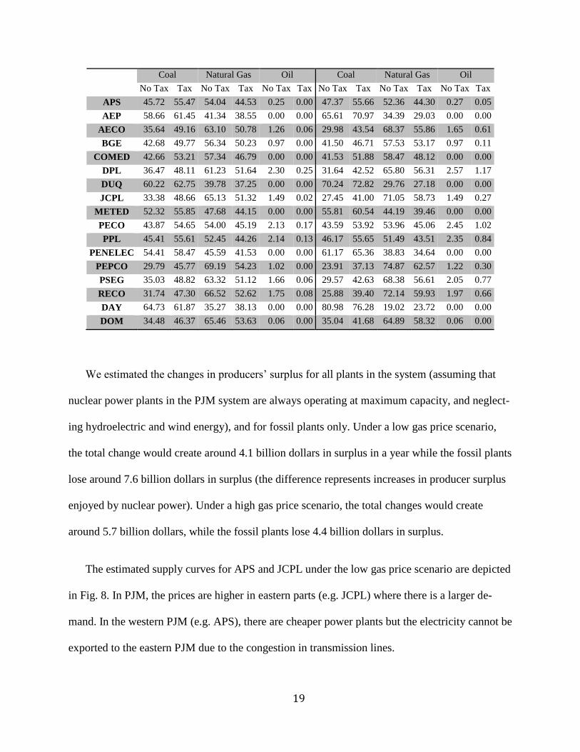
19

Coal Natural Gas Oil Coal Natural Gas Oil

No Tax Tax No Tax Tax No Tax Tax No Tax Tax No Tax Tax No Tax Tax

APS 45.72 55.47 54.04 44.53 0.25 0.00 47.37 55.66 52.36 44.30 0.27 0.05

AEP 58.66 61.45 41.34 38.55 0.00 0.00 65.61 70.97 34.39 29.03 0.00 0.00

AECO 35.64 49.16 63.10 50.78 1.26 0.06 29.98 43.54 68.37 55.86 1.65 0.61

BGE 42.68 49.77 56.34 50.23 0.97 0.00 41.50 46.71 57.53 53.17 0.97 0.11

COMED 42.66 53.21 57.34 46.79 0.00 0.00 41.53 51.88 58.47 48.12 0.00 0.00

DPL 36.47 48.11 61.23 51.64 2.30 0.25 31.64 42.52 65.80 56.31 2.57 1.17

DUQ 60.22 62.75 39.78 37.25 0.00 0.00 70.24 72.82 29.76 27.18 0.00 0.00

JCPL 33.38 48.66 65.13 51.32 1.49 0.02 27.45 41.00 71.05 58.73 1.49 0.27

METED 52.32 55.85 47.68 44.15 0.00 0.00 55.81 60.54 44.19 39.46 0.00 0.00

PECO 43.87 54.65 54.00 45.19 2.13 0.17 43.59 53.92 53.96 45.06 2.45 1.02

PPL 45.41 55.61 52.45 44.26 2.14 0.13 46.17 55.65 51.49 43.51 2.35 0.84

PENELEC 54.41 58.47 45.59 41.53 0.00 0.00 61.17 65.36 38.83 34.64 0.00 0.00

PEPCO 29.79 45.77 69.19 54.23 1.02 0.00 23.91 37.13 74.87 62.57 1.22 0.30

PSEG 35.03 48.82 63.32 51.12 1.66 0.06 29.57 42.63 68.38 56.61 2.05 0.77

RECO 31.74 47.30 66.52 52.62 1.75 0.08 25.88 39.40 72.14 59.93 1.97 0.66

DAY 64.73 61.87 35.27 38.13 0.00 0.00 80.98 76.28 19.02 23.72 0.00 0.00

DOM 34.48 46.37 65.46 53.63 0.06 0.00 35.04 41.68 64.89 58.32 0.06 0.00

We estimated the changes in producers’ surplus for all plants in the system (assuming that

nuclear power plants in the PJM system are always operating at maximum capacity, and neglect-

ing hydroelectric and wind energy), and for fossil plants only. Under a low gas price scenario,

the total change would create around 4.1 billion dollars in surplus in a year while the fossil plants

lose around 7.6 billion dollars in surplus (the difference represents increases in producer surplus

enjoyed by nuclear power). Under a high gas price scenario, the total changes would create

around 5.7 billion dollars, while the fossil plants lose 4.4 billion dollars in surplus.

The estimated supply curves for APS and JCPL under the low gas price scenario are depicted

in Fig. 8. In PJM, the prices are higher in eastern parts (e.g. JCPL) where there is a larger de-

mand. In the western PJM (e.g. APS), there are cheaper power plants but the electricity cannot be

exported to the eastern PJM due to the congestion in transmission lines.

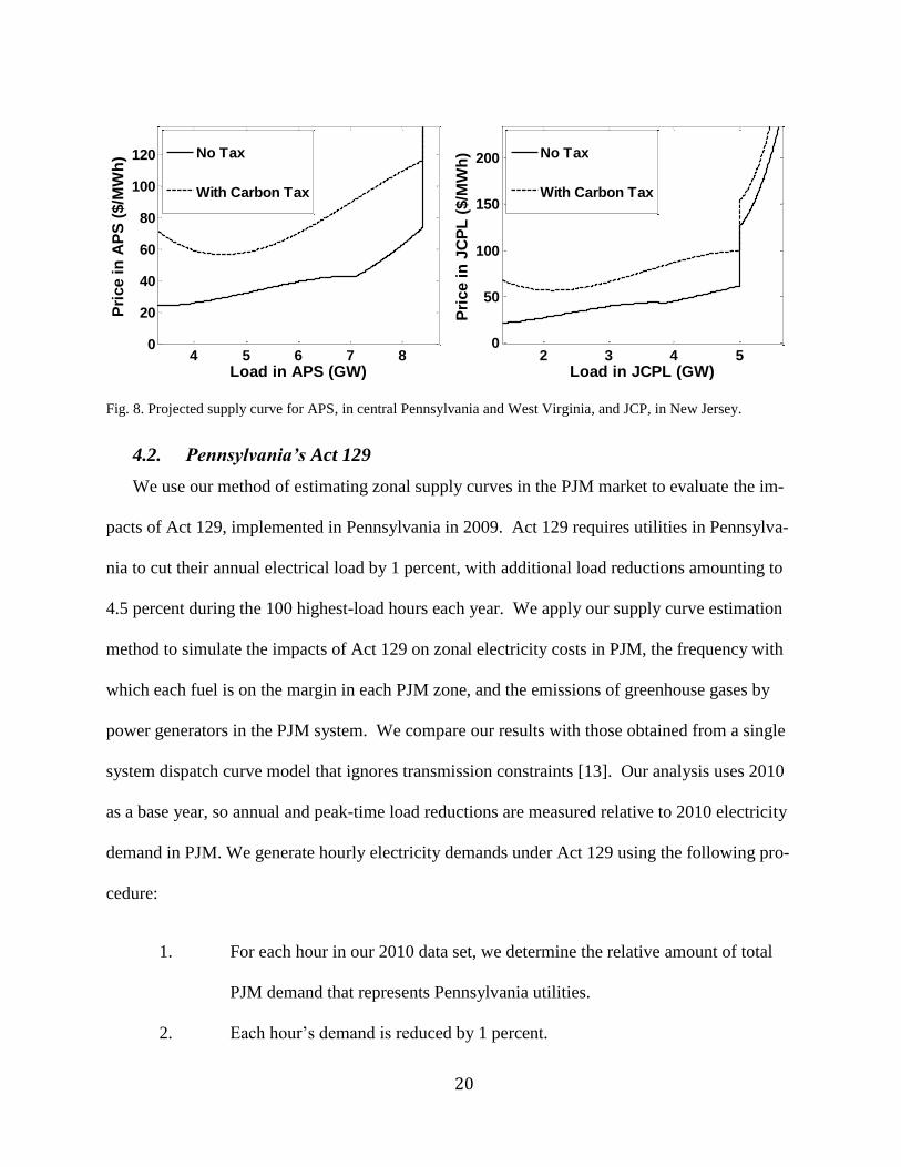
20

Fig. 8. Projected supply curve for APS, in central Pennsylvania and West Virginia, and JCP, in New Jersey.

4.2. Pennsylvania’s Act 129

We use our method of estimating zonal supply curves in the PJM market to evaluate the im-

pacts of Act 129, implemented in Pennsylvania in 2009. Act 129 requires utilities in Pennsylva-

nia to cut their annual electrical load by 1 percent, with additional load reductions amounting to

4.5 percent during the 100 highest-load hours each year. We apply our supply curve estimation

method to simulate the impacts of Act 129 on zonal electricity costs in PJM, the frequency with

which each fuel is on the margin in each PJM zone, and the emissions of greenhouse gases by

power generators in the PJM system. We compare our results with those obtained from a single

system dispatch curve model that ignores transmission constraints [13]. Our analysis uses 2010

as a base year, so annual and peak-time load reductions are measured relative to 2010 electricity

demand in PJM. We generate hourly electricity demands under Act 129 using the following pro-

cedure:

1. For each hour in our 2010 data set, we determine the relative amount of total

PJM demand that represents Pennsylvania utilities.

2. Each hour’s demand is reduced by 1 percent.

4 5 6 7 80

20

40

60

80

100

120

Load in APS (GW)

Pri

ce i

n A

PS

($/M

Wh

)

No Tax

With Carbon Tax

2 3 4 50

50

100

150

200

Load in JCPL (GW)

Pri

ce i

n J

CP

L (

$/M

Wh

)

No Tax

With Carbon Tax

21

3. In the top 100 hours of demand, each hour’s demand is reduced by an addition-

al 4.5 percent.

Given our new set of hourly PJM demands, adjusted to reflect successful implementation of

Act 129, hourly market-clearing prices and generator dispatch are obtained by determining the

intersection between the short-run supply curve and a vertical demand curve at each hour’s level

of demand. The same procedure is used to obtain hourly market-clearing prices and generator

dispatch for our baseline case, based on the PJM market in 2010.

Our estimates of Act 129’s impact generated using the single dispatch curve model projects

that total electricity costs in the PJM territory would decline by $150 million on an annual basis

following the successful implementation of Act 129. Using plant-level average emissions data

from the e-GRID database, we calculate that Act 129 reduces annual carbon dioxide emissions in

the PJM territory by 2.9 million tons. For simplicity, we assumed that APS meets Act 129 de-

mand reduction goals in its entire territory. The fuel prices in our estimation are the ones pre-

sented as the low gas price scenario (Table 2).

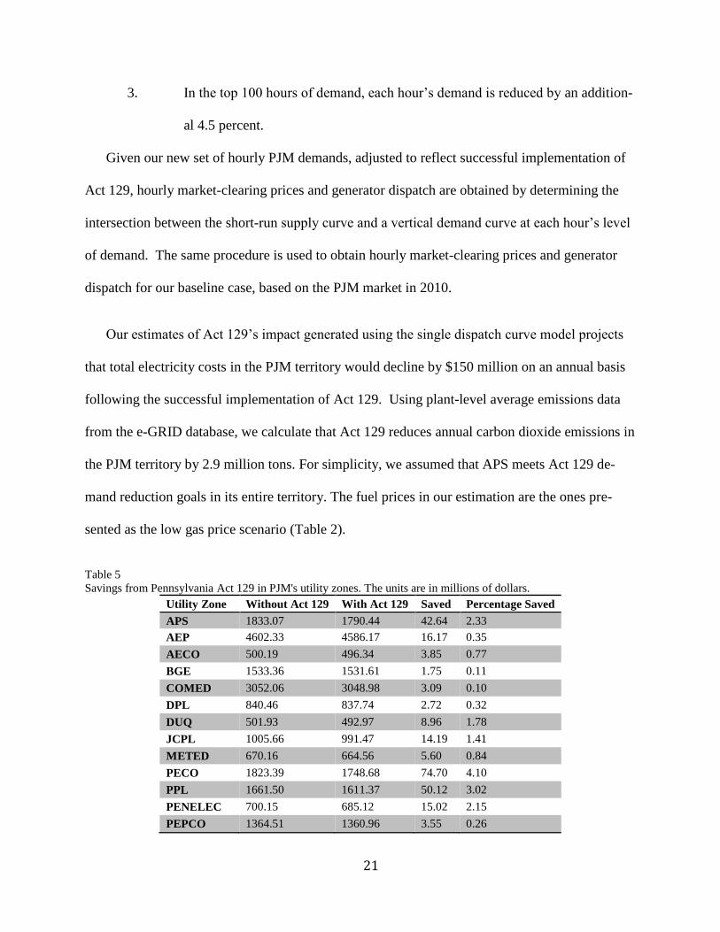
Table 5

Savings from Pennsylvania Act 129 in PJM's utility zones. The units are in millions of dollars.

Utility Zone Without Act 129 With Act 129 Saved Percentage Saved

APS 1833.07 1790.44 42.64 2.33

AEP 4602.33 4586.17 16.17 0.35

AECO 500.19 496.34 3.85 0.77

BGE 1533.36 1531.61 1.75 0.11

COMED 3052.06 3048.98 3.09 0.10

DPL 840.46 837.74 2.72 0.32

DUQ 501.93 492.97 8.96 1.78

JCPL 1005.66 991.47 14.19 1.41

METED 670.16 664.56 5.60 0.84

PECO 1823.39 1748.68 74.70 4.10

PPL 1661.50 1611.37 50.12 3.02

PENELEC 700.15 685.12 15.02 2.15

PEPCO 1364.51 1360.96 3.55 0.26

22

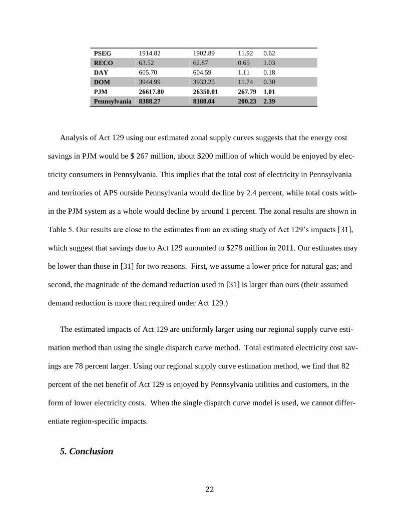
PSEG 1914.82 1902.89 11.92 0.62

RECO 63.52 62.87 0.65 1.03

DAY 605.70 604.59 1.11 0.18

DOM 3944.99 3933.25 11.74 0.30

PJM 26617.80 26350.01 267.79 1.01

Pennsylvania 8388.27 8188.04 200.23 2.39

Analysis of Act 129 using our estimated zonal supply curves suggests that the energy cost

savings in PJM would be $ 267 million, about $200 million of which would be enjoyed by elec-

tricity consumers in Pennsylvania. This implies that the total cost of electricity in Pennsylvania

and territories of APS outside Pennsylvania would decline by 2.4 percent, while total costs with-

in the PJM system as a whole would decline by around 1 percent. The zonal results are shown in

Table 5. Our results are close to the estimates from an existing study of Act 129’s impacts [31],

which suggest that savings due to Act 129 amounted to $278 million in 2011. Our estimates may

be lower than those in [31] for two reasons. First, we assume a lower price for natural gas; and

second, the magnitude of the demand reduction used in [31] is larger than ours (their assumed

demand reduction is more than required under Act 129.)

The estimated impacts of Act 129 are uniformly larger using our regional supply curve esti-

mation method than using the single dispatch curve method. Total estimated electricity cost sav-

ings are 78 percent larger. Using our regional supply curve estimation method, we find that 82

percent of the net benefit of Act 129 is enjoyed by Pennsylvania utilities and customers, in the

form of lower electricity costs. When the single dispatch curve model is used, we cannot differ-

entiate region-specific impacts.

5. Conclusion

23

Analysis of electricity policies often requires understanding the effects of transmission con-

straints, which can be very complex. Incorporating transmission-system in engineering models

requires detailed information that is neither publicly available nor practical to use for many

economists and policy analysts. Many existing analyses thus abstract from transmission con-

straints. While this assumption makes modeling more tractable, it can underestimate the impacts

of electricity policies, sometimes by substantial margins. Moreover, abstraction from transmis-

sion constraints prevents the estimation of location-specific impacts. We develop a method to

estimate zonal prices in a transmission-constrained electricity markets. Our method also esti-

mates the marginal fuel based on zonal load and the total demand in the market. It can also detect

when a mixture of two fuels is on the margin. Our model is particularly useful when the distribu-

tional impacts of a policy are of special interest.

We applied our model to the seventeen utility zones in the PJM footprint and calculated the

fuzzy zonal thresholds where the marginal fuel switches. Our results show the sensitivity of the

marginal fuel to the zonal and system loads. We found that the price of electricity in PJM is

mostly driven by natural gas prices, although in some zones coal-fired power plants are on the

margin during the majority of hours. We simulated a carbon tax of $35 per ton in PJM and

found that such a policy would increase the prices by 47 to 89 percent in PJM. Such a carbon tax

would increase the influence of coal on formation of electricity prices and reduce the CO2 emis-

sions by 7.2 to 10.6 percent. Our example analysis of Pennsylvania’s Act 129 shows that compli-

ance with Act 129 demand-reduction targets lowers total electric generation costs in Pennsylva-

nia by 2.4 percent. We estimate the total cost reduction in PJM to be around 1 percent which

translates to $267 million. While the assumption that transmission constraints can be ignored

24

makes policy models more tractable, our analysis of Pennsylvania Act 129 suggests that these

models may underestimate the impacts of electricity policies.

In order to be able to construct this model, there is an essential need for data. It should be

noted that, price and load data is not publically available for some power systems such as South-

ern Company. Moreover, similar to any statistical method, the accuracy of the results relies on

the consistency of the historical data. Any significant structural change in the system, such as

major new transmission lines, would affect the reliability of the model.

Appendix: Correcting for Electricity Price Over-Estimation in the Fuzzy band

For the sake of simplicity assume that the marginal fuel is just a function of zonal load.

Moreover assume that the electricity price is a linear function of load in each segment. Fig. A1-a

shows such a condition when the difference between natural gas and coal price is large enough

that there is no overlap between segments of the zonal supply curve (the threshold between the

coal and gas segments is a deterministic line). At the threshold the most expensive coal fired

power plant sets the price at p1. Now assume that natural gas prices drop to a lower level result-

ing in a fuzzy band between the coal and natural gas segments of the zonal supply curve. The

price is still equal to p1 but it could be set either by a high-cost coal plant with a marginal cost of

p1 at the relevant level of production, or a low-cost natural gas plant, also with a marginal cost of

p1 at the relevant level of production. This situation is shown in Fig. A1-b.

In the fuzzy band, either coal or gas could be the marginal fuel, but in either case the prevail-

ing price should be p1. The estimation problem arises when projecting the coal portion of the

supply curve to the upper boundary of the fuzzy band. Within the fuzzy band, both the coal and

gas segments of the supply curve would predict a price of p1. But on the boundary of the fuzzy

25

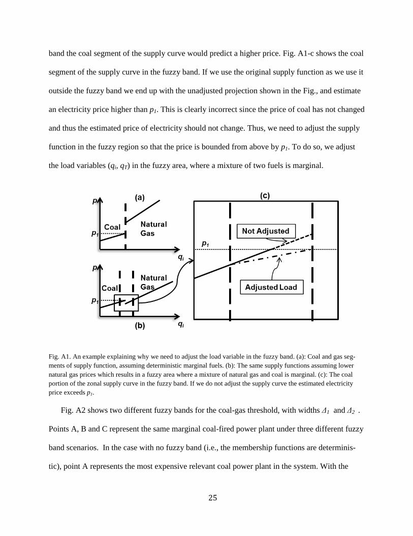
band the coal segment of the supply curve would predict a higher price. Fig. A1-c shows the coal

segment of the supply curve in the fuzzy band. If we use the original supply function as we use it

outside the fuzzy band we end up with the unadjusted projection shown in the Fig., and estimate

an electricity price higher than p1. This is clearly incorrect since the price of coal has not changed

and thus the estimated price of electricity should not change. Thus, we need to adjust the supply

function in the fuzzy region so that the price is bounded from above by p1. To do so, we adjust

the load variables (qi, qT) in the fuzzy area, where a mixture of two fuels is marginal.

Fig. A1. An example explaining why we need to adjust the load variable in the fuzzy band. (a): Coal and gas seg-

ments of supply function, assuming deterministic marginal fuels. (b): The same supply functions assuming lower

natural gas prices which results in a fuzzy area where a mixture of natural gas and coal is marginal. (c): The coal

portion of the zonal supply curve in the fuzzy band. If we do not adjust the supply curve the estimated electricity

price exceeds p1.

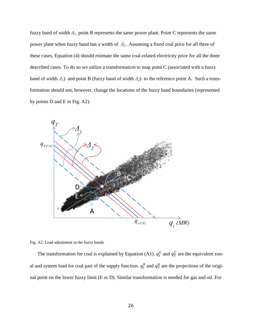
Fig. A2 shows two different fuzzy bands for the coal-gas threshold, with widths Δ1 and Δ2 .

Points A, B and C represent the same marginal coal-fired power plant under three different fuzzy

band scenarios. In the case with no fuzzy band (i.e., the membership functions are determinis-

tic), point A represents the most expensive relevant coal power plant in the system. With the

26

fuzzy band of width Δ1 , point B represents the same power plant. Point C represents the same

power plant when fuzzy band has a width of Δ2 . Assuming a fixed coal price for all three of

these cases, Equation (4) should estimate the same coal-related electricity price for all the three

described cases. To do so we utilize a transformation to map point C (associated with a fuzzy

band of width Δ1) and point B (fuzzy band of width Δ2) to the reference point A. Such a trans-

formation should not, however, change the locations of the fuzzy band boundaries (represented

by points D and E in Fig. A2).

Fig. A2. Load adjustment in the fuzzy bands

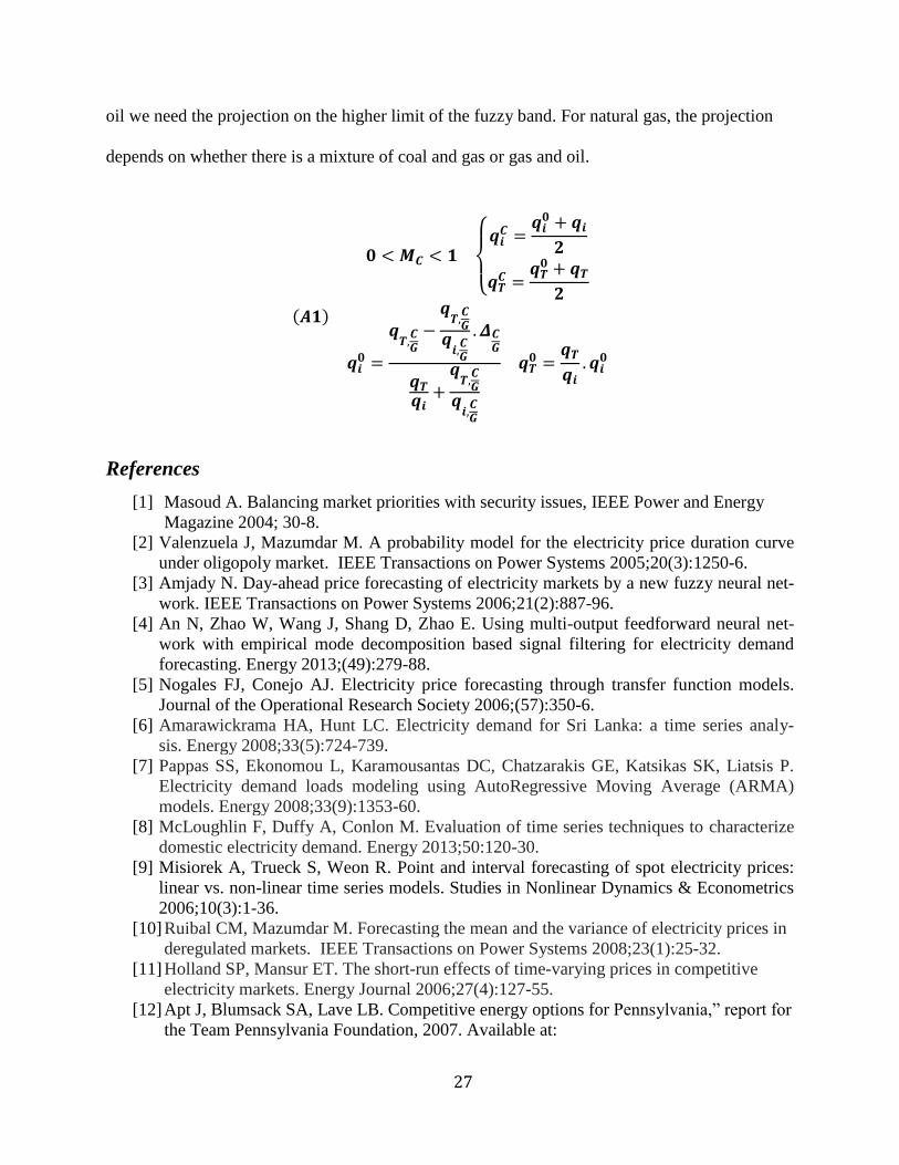
The transformation for coal is explained by Equation (A1). 𝑞𝑖𝐶 and 𝑞𝑇

𝐶 are the equivalent zon-

al and system load for coal part of the supply function. 𝑞𝑖0 and 𝑞𝑇

0 are the projections of the origi-

nal point on the lower fuzzy limit (E or D). Similar transformation is needed for gas and oil. For

qT,C/G

qi,C/G

Δ1

Δ2

C B

A

E

D

qi (MW)

qT

(MW)

27

oil we need the projection on the higher limit of the fuzzy band. For natural gas, the projection

depends on whether there is a mixture of coal and gas or gas and oil.

(𝑨𝟏)

𝟎 < 𝑴𝑪 < 𝟏

{

𝒒𝒊𝑪 =

𝒒𝒊𝟎 + 𝒒𝒊𝟐

𝒒𝑻𝑪 =

𝒒𝑻𝟎 + 𝒒𝑻𝟐

𝒒𝒊𝟎 =

𝒒𝑻,𝑪𝑮−

𝒒𝑻,𝑪𝑮

𝒒𝒊,𝑪𝑮

. 𝜟𝑪𝑮

𝒒𝑻𝒒𝒊+

𝒒𝑻,𝑪𝑮

𝒒𝒊,𝑪𝑮

𝒒𝑻𝟎 =

𝒒𝑻𝒒𝒊. 𝒒𝒊𝟎

References

[1] Masoud A. Balancing market priorities with security issues, IEEE Power and Energy

Magazine 2004; 30-8.

[2] Valenzuela J, Mazumdar M. A probability model for the electricity price duration curve

under oligopoly market. IEEE Transactions on Power Systems 2005;20(3):1250-6.

[3] Amjady N. Day-ahead price forecasting of electricity markets by a new fuzzy neural net-

work. IEEE Transactions on Power Systems 2006;21(2):887-96.

[4] An N, Zhao W, Wang J, Shang D, Zhao E. Using multi-output feedforward neural net-

work with empirical mode decomposition based signal filtering for electricity demand

forecasting. Energy 2013;(49):279-88.

[5] Nogales FJ, Conejo AJ. Electricity price forecasting through transfer function models.

Journal of the Operational Research Society 2006;(57):350-6.

[6] Amarawickrama HA, Hunt LC. Electricity demand for Sri Lanka: a time series analy-

sis. Energy 2008;33(5):724-739.

[7] Pappas SS, Ekonomou L, Karamousantas DC, Chatzarakis GE, Katsikas SK, Liatsis P.

Electricity demand loads modeling using AutoRegressive Moving Average (ARMA)

models. Energy 2008;33(9):1353-60.

[8] McLoughlin F, Duffy A, Conlon M. Evaluation of time series techniques to characterize

domestic electricity demand. Energy 2013;50:120-30.

[9] Misiorek A, Trueck S, Weon R. Point and interval forecasting of spot electricity prices:

linear vs. non-linear time series models. Studies in Nonlinear Dynamics & Econometrics

2006;10(3):1-36.

[10] Ruibal CM, Mazumdar M. Forecasting the mean and the variance of electricity prices in

deregulated markets. IEEE Transactions on Power Systems 2008;23(1):25-32.

[11] Holland SP, Mansur ET. The short-run effects of time-varying prices in competitive

electricity markets. Energy Journal 2006;27(4):127-55.

[12] Apt J, Blumsack SA, Lave LB. Competitive energy options for Pennsylvania,” report for

the Team Pennsylvania Foundation, 2007. Available at:

28

http://wpweb2.tepper.cmu.edu/ceic/papers/Competitive_Energy_Options_for_Pennsylva

nia.htm

[13] Newcomer A, Blumsack SA, Apt J, Lave LB, Morgan MG. Short run effects of a price

on carbon dioxide emissions from US electric generators. Environmental Science &

Technology 2008;42(9):3139-44..

[14] Newcomer A, Apt J. Near-term implications of a ban on new coal-fired power plants in

the United States. Environmental science & technology 2009;43(11):3995-4001.

[15] Blumsack, S. Electric rate design and emissions reductions. In Proc. of IEEE Power and

Energy Society General Meeting 2009, Calgary AB.

[16] Dowds J, Hines P, Farmer C, Watts R. Estimating the impact of electric vehicle charging

on electricity costs given electricity-sector carbon cap. Transportation Research Record.

Journal of the Transportation Research Board 2010:2191(1):43-9.

[17] Dowds J, Hines P, Blumsack S. Estimating the impact of fuel-switching between liquid

fuels and electricity under electricity-sector carbon-pricing schemes. Socio-Economic

Planning Sciences 2013;47(2):76–88.

[18] Borenstein S, Bushnell JB, Wolak FA. Measuring market inefficiencies in California’s

restructured wholesale electricity market. The American Economic Review 2002;

92(5):1376-404.

[19] Joskow P, and Kahn E. Identifying the exercise of market power: refining the estimates.

Technical report 2001.

[20] US Environment Protection Agency. The Emissions & Generation Resource Integrated

Database (eGRID). Available at: www.epa.gov/egrid

[21] Fisk JM. The right to know? state politics of fracking disclosure. Review of Policy Re-

search 2013;30(4):345–65.

[22] Holladay JS, LaRiviere J. The effect of abundant natural gas on air pollution from elec-

tricity production. Working Paper 2013.

[23] Sahraei-Ardakani M, Blumsack S, Kleit A. Zonal supply curve estimation in transmis-

sion-constrained electricity markets. Available at SSRN 2011;

http://ssrn.com/abstract=1937411

[24] Sahraei-Ardakani M, Blumsack, SA, Kleit A. Distributional impacts of state-level ener-

gy efficiency policies in regional electricity markets. Energy Policy 2013; 49:365-72.

[25] Kleit A, Blumsack SA, Lei Z, Hutelmyer L, Sahraei-Ardakani S, Smith S. Impacts of

electricity restructuring in rural Pennsylvania. The Center for Rural Pennsylvania 2011.

[26] Govindarajan A, Blumsack SA. Equilibrium modeling of combined heat and power de-

ployment. In Proc. of 32nd

USAEE North American Conference, 2012.

[27] Hansen N, Muller S, Koumoutsakos P. Reducing the time complexity of the derandom-

ized evolution strategy with covariance matrix adaptation (CMA-ES). Evolutionary

Strategy 2003;11(1):1-18.

[28] Hansen N, Ostermeier A. Completely Derandomized Self-Adaptation in Evolution Strat-

egies. Evolutionary Computation 2001;9(2):159-95.

[29] Schnoor, J. Responding to Climate Change with a Carbon Tax. Environmental science &

technology 2014.

[30] Spees K, and Lave L. Demand response and electricity market efficiency. The Electricity

Journal 2007; 20(3):69-85.

29

[31] PennFuture. Pennsylvania 2013-2018 Energy Efficiency Goals. 2011; Available at:

http://www.pennfuture.org/UserFiles/File/FactSheets/Report_Act129goals_20111220.pd

f