Estimation of Lateritic-Type Orebodies

By A. G. JOURNEL,' aM CH. HUIJBREGTS

S¥NOPS[S

Special problems' arise in the evaluation of lateritic-type orebodies (Ni.Co, bauxite) or, more senerally, orebodles affected by surface weathering. In this type of orcbody, the vertical grade distribution shows. fwm the hangingwaU downwards, a systematic increase followed sometimes by a certain decrease, or vice-versa. These trends appear together with irregular variations from one drill hole to the other. '

The problem is to characterize It vcctica.l structure that is representative nol only of the drill hole but of an entire pane.! or zone of infl uence., in order to define: mineable thicknesses for giveo cut·oIT grades. The vertical grade distribution observed on lhe drillhole is replaced by a DeW curve, called 'derive' (drift), which is computed by 'universall:riging'.

Once the vertical study is completed, new '$«'Vice-variables' arc defined in the borizootal plane, such as mineable thiclmess and the corresponding average grade, economical functions (combination of the grades of several minerals). Tho local and global estimation of these variables can then be performed by a simple bl-dimensional krisioa plan. The global cstimlU!on is summed up by several tonnage-cut-off grade curves.

The practk:al vllluation according to the above scheme of a New Caledonian lateritlc nickel orebody is pf'C$C:oted.

INTRODUCTION

A great number of orebodies affected by surface weathering processes show a particular direction in trend which should be rustinguished when estimating. This characteristic direction is generally vertical, but whatever it lOay be (for example, radial from a pipe) the methodology described here wowd apply. witb some simple modifications. For greater clarity, the method is demonstrated by means of a practical valuation of the Prony orebody (New Caledonia). This method has been applied also to lateritic-type bauxite orebodics (Les Baux in France) and is being applied to a phosphate orebody in Togo (West Africa), For reasons of security all data in thi! paper have been multiplied by a factor.

The ProllY orebody appears as a nickd-bearing fonnalion of surface-weathered basic rocks. From lop to bottom, tbe following are distinguished:

(i) • COHUginOU' oop,

(ii) different types oC ore, from the laterites to the magnesian. silicated products down to the garnierites which are at the contact of the bed-rock: peridotites.

The available inCormati.on is derived Crom several vertical boreho[es, analyzed at each meter, and set

(i) aloog , "gola< squ"" odd (400 m) 0'"'' th, whol, orcbody, of about 20 km2,

(H) along two crosses with a regular 20 tU spacing, to define the small-scale structures.

With this information the ore reserve valuatiOQ of the deposit is performed. taking into account the two selection criteria, namely, nickel cut-off grade, t c. and limit OD mineable thickness PLo

VERTICAL REGIONALIZATION

Existellce of a drift

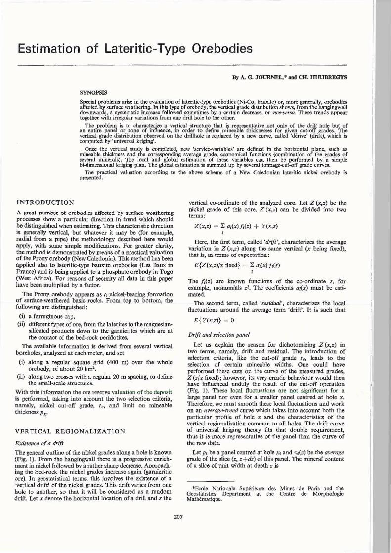
The general outline of the nickel grades along a hole is known (Fig. 1). From the hangingwall there is a progressive enr.ich­ment ill nickel followed by a rather sharp decrease. Approach­iug the bed-rock the nickel grades increase again (garnieritic ore). In geostatistical terms, this involves the existence of a 'vertical drift' of the nickel grades. This drift varies from one hole to another, so that it will be collSidered as a random drift. Let x denote the borizontallocation of a drill and:z the

207

vertical co·ordioate of the analyzed core. Let Z (x,z) be the nickel grade of tbis core. Z (x,z) can be divided ioto two terms:

Z(x,z) - I: ar(x)fI(z) + Y(x,z)

Here, the first term, called 'drift', characterizes tbe average variation io Z (x,t) along the same vertical (x being fixed), iliat is, in terms of expectation:

E{Z(x,z)/x fixed} = Z a/ex) Nz) , The f«z) are known functions of the ClH>rdinate z, for example, monomials ;1. The coefficients a«x) must be esfi­maled.

1bc second tenn, called 'residuaF, charncterizes the local liuctuations around the average term ·drift'. It is such that

E{Y(x,z)) - 0

Drift and selection panel

Let us explain lbe reason for dicbotomizing Z (x,z) in two terms, namely, drift and .res.idual. The introduction of selection criteria, like tbe cut-<lff grade t c, leads to the selection of certaia mineable widths, Oae could have performed these cuts on the curve of the measured grades, Z (z/x fixed); however, its very erratic behaviour would then bnve influenced unduJy the result of the cut-<lff operation (Fig. 1). These loca1 fluctuations are not Significant for a large paocl Dor even for a smaller panel centred at hole x. Therefore. we must smooth these local fluctuations and work on an average-trend curve which takes into account both the particular profile of hole x and the characteristics of the vertical regionalization common to all holes. The drift curve of universal kriging theory fits that double requirement, thus it is more represeotative of the paoel than the curve of the raw data.

Let JJj be a panel ccntred at hole x, and "\j(;) be the average grade of the slice (z, z + dz) of this panel. The mineral content or a slice of unit width at depth :z is

+Ecole Nationale Su~rieure des Mines de Paris and the Geoslatistics Department at the Centre de Morphologie Mathtmatique.

(pf) '\"f(Z) = f Z(x,z)dx - Lfr(z) f a,(x)dx + f Y(x,z)dx ~ l Pf P'

The cut-off grade la must be applied to the curve '\"/(l') and not to the raw data Z (Xi,Z) curve. To define the character of the 'residual fluctuation', that is, of the tcnn Y(x,z), we can considcr its range as being very small in comp."lrison with the horizontal dimcnsions of panel p/..

Hence,

f Y(x,z) dx ::::: E{y(x,z)} = o. p,

Next, we must estimate the integral of the drift. Accurate estimation of this integml is possible as long as the character­istics of the coefficients OAX) are known, particularly covaflances such as E {odx) a~x+h)}. Generally, the available grid of holes is too wide to permit a correct e.~timatioll of these covariances.

Our basic hypothesis is {hat the elementary panel, on which the cut-off t ~ grade operation is to be performed, is defined so that its horizontal dimensions are SO small that variations in the coefficients oI(x) across it are negligible. Hence,

1't(z) ~ 1; ft(z) o,(x.).

It is therefore sufficient to estimate the drift curve correspon­ding to the central hole x(. This estimation is performed by means of universal kriging, Matheron (1969), and needs only the knowledge of the vertical regionalizatioll of the grades, thllt is, Z (z/x f'ixod). This regionalization is known from experiment.

40O ....

1 J 08 09' • ••• •. , 0

• 0

15 .... m.

" ••

.. 1r ..........

Fig. 1.

208

It may be noted that the same hypothesis underlies the classical process which consists of cutting the raw data curve Z (Xf,Z) of the borehole, Xt. In tllis case the whole Z (x/,z) curve is assumed to be constant throughout the elementary paneJ Pi and not only its drift or 'average trend'. Moreover, in the classiCl11 approach, panel p, coincided with the grid panel P i centred On hole Xf, that is, it was a large panel say 400 x 400 m in this study. It is evident from Fig. j that the dimensions of the grid panel are generally much too large to verify the above hypothesis. Holes DB and D9, some 400 Ol apart, are essentially different . The dimensions of the elementary panels are limitcd to 20 X 20 m, as 20 ID is the hole spacing of our small-scale crosses. The raw data curves for tbe two boles drilled 20 m apart, 09 and D9', are st ill quite different, tbough the drift curves are almost identical.

Cuts and ser~/ce ~ariables

We adopted the marginal definition of the cut-off grade I r, that is, a width with a te average grade in nickel which would just payoff its cost of mining and dressing. Thus, for le ~ 0.8 per cent nickel, we would keep a mineable thickness of 7.6 m for the 20 X 20 m panel ceotred on hole D9 (Fig. I). According to the particular conditions of each ombody, the political system of the owner country etc., alternative defini­tions of the cut-olT grade could be adopted.

In any event, at this stage of the valuation, the two cuts, grade tt and mineable thickness limit, Po must not be ntixed. Indeed, it will be seen that the panel considered last is not the 20 x 20 m elementary panel, but a much larger one. The selective criterion Pr. will be applied to (hat last panel.

20m

., O. d •• U

, . 1.'m

'0

..

So, for each cut-off grade l e. we define a certain number of variabtes which we will call service-I'ariables. These service­variables are representative of the elementary 20 X 20 m panel PI centred at hole Xt. Wc, shaH write them v(XI), For example. they represent:

(i) the stripping thickness, (ii) the mioeable thickness, and

(iii) the corresponding quantity of metal.

The cut-o{f is perfonned on an estimated drift curve and not on the actual but unknown drifl curve. As a result the service variables are affected by an error in estimation, the variance of which eau be calculated. It has been found that for stripping thickness and mineable thickness the relative standard deviation is about 15 per cent aod for the quantity of nickel is about 10 perceJll. Thus, thecstimate5coocerningeven those elementary panels which are pierced by a central hole, have, at best, a relative standru'd deviation of 10 per cent. As the holes tU'e placed on a 400 X 400 m grid, we expect the local estimation of less well-located elemeotary panels to be very bad. Anyway, these new estimations require horizontal extrapolation of known values to unknown values, that is, the introduction of thc stl.1dy of horizontal regionalizations.

HORIZONTAL REGIONALlZATIONS

Horizontal v(Iriograms

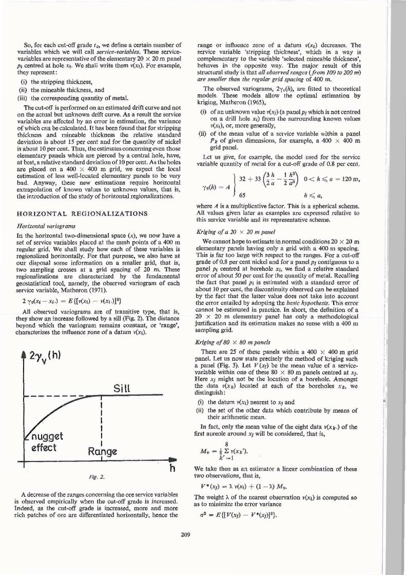
In the horizontal two-dimensional space (x) , wo now have a set of service vru::iables placed at the mesh poiots of a 400 lD regular grid. We shall study how cach of these variables is regionalized horizontaUy. For that purpose, we also have al our disposal some information on a smaller grid, that is, two sampling crosses at a grid spacing of 20 m. Theso regionalizations are characterized by the fundamental geostatistical tool. namely. the observed variogram of each service variable, Mathcrou (1971).

2 yV<~ - Xj .) = E ([v(Xt) - V(XI.W}

All observed variograms are of transitive type, that is, they mow an increase followed by a sill (Pig. 2). The distance beyond which the variogram remains constant, or 'range', characterizes the influence zone of a datum v(XI).

Sill - - - - - -:.;-,.-,---':";';';""--

I I I I I I

Range

Fig. 2. h

A decrease of the ranges concerning tne ore service variables is observed empirically wben the cut-off grade is increased. Indeed, as the cut-off grade is increased, more and more ricll patches of ore are differentiated horizontally, bence tbe

209

range or influencc zone of a datum v(x,) decreases. The service variable 'stripping thickness', which in a way is complementary to tne variable 'selected mineable thickness', behaves in the opposite way. The major result of this structural study is tbat all observed ranges (from 100 to 200 m) are smaller titan the regular grid spacing of 400 m.

The observed variograms, 2y~(h) , are filted to theoretical models. These models allow the optimal estimation by kriging, Matheron (196:5),

(i) of an unknown value y(Xj) (a panclPi which is Dot centred 00 a dr ill hole x,) from the surrounding known values v(Xi), or, more generally,

(ii) of the mean value of a service variable within a panel p } of given dimensions, for example, a 400 x 400 m grid panel.

Let us give, for example, the model used for the service variable quantity of metal for a cut-off grade of 0.8 per cent.

1 J2 + 33 (-2

3 ~ --21 h:) 0 < IT. ::;;;; 0 = nOm,

YtAh) = A u er

6$ h ::;;;; a,

where A is a multiplicative factor. This is a spherical scheme. All va lues g iven later as examples are cxpressed relative to this service variable and its representa tive scheme,

Krig lng oJ a 20 X 20 m panel

We cannot hope to estimate in normal conditions 20 X 20 m elementary panels baving only a grid with a 400 m spacing. TIllS is far too large wi th respect to the ranges. For a cut-off grade of 0.8 per cent nickel and for a panel Pt contiguous to a panel PI. centred at borehole Xl, we find a relative standard error of about 50 per cent for the quantity of metal. Recalling the fact that paoeJ Pi is estimated with a standard error of about 10 per cent, the discontinuity obscrved can be exptained by the fact that tbe latter value does not take into account the error entailed by adopting the basie hypotltesis. This error cannot be estimated in practice. In short, the definition of a 20 x 20 m elementary panel has only a methodological justification and its estimation makes no sense with a 400 m sampling grid.

Krigihg oJ 80 x 80 m panels

There are 25 of tbese panels within a 400 x 400 m grid panel. let us now state precisely the method of kriging such a panel (Fig, 3). Let V(Xj) be the mean value of a service­variable within one of these 80 x 80 m panels centred at XI. He", XI miiht not be tbe location Qf a borehole, Amongst the d:ua P(Xk) located at each of the borehoJes x } , we distinauish:

(i) the datum v(Xj) Dearest to XI and (ii) the set of the other data which contribute by means of

their arithmetic mean.

In fact, only the mean value or the cight data v(Xl") of tbe first aureole around '''(1 will be considered, that is,

8 M ., - t E y(Xk' ).

k' =>< 1

We take then as an estimator a linear combination of these two observations, that is,

V·(XJ} - A f(xt) + (J - A) M ,.

The weight A of the nearest observation vex,) is computed so as to minimize the error variance

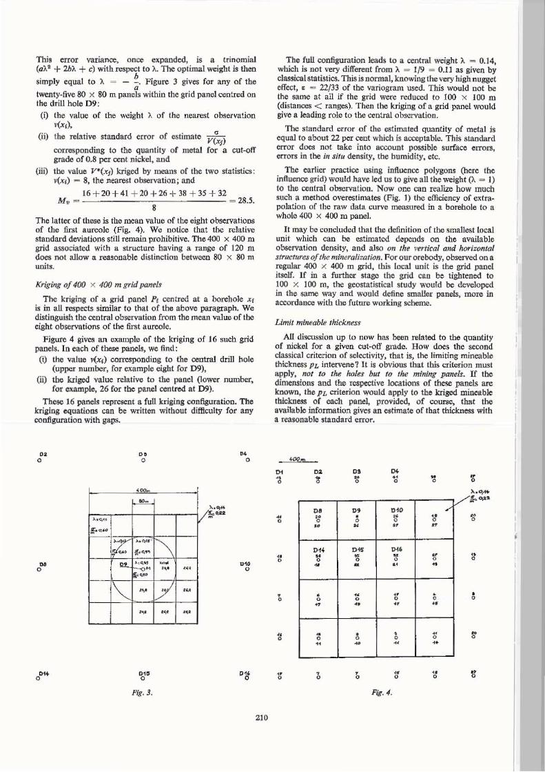
This error variance, once expanded, is a trinomial (a>.1 + 2b>. + c) with re!lpoct to A. 1be optimal weight is then

simply equal to A = - ~. Figure 3 gives for any of the a

twenty-five 80 x 80 m panels within the grid panel centred on the drill hole D9:

0) the value of the weight A of the nearest observation I{X,).

(ii) the relative standard error of estimate

corresponding to the quantity of metal grade of 0.8 per cent nickel. and

a Vex,) for a

(iii) tbe value V·(.q) kriged by means of the two statistics : V(X,) - 8, the nearest observation; and

16 + 20 + 41 + 20 + 26 + 3S + 35 + 32 Mv - = 28.5.

8 The latter of these is the mean value of the eight observations of tile first aureole (Fig. 4). We notice that the relative standard deviations still remain prohibitive. The 400 x 400 m grid associated with a structure having a range of 120 m does not allow a reasonable distinction betWCCll 80 x SO m umlS.

Kriging of 400 x 400 m grid pant/~

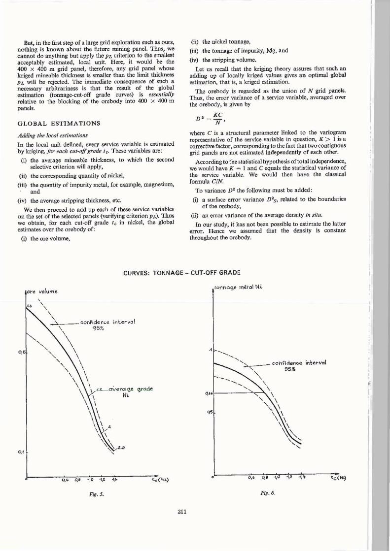
The kriging of a grid panel P, centred at a borehok: XI

is in a U respects similar to that of the above paragraph. We distinguish the central observation from the mean value of the eight observations of the first aureole.

Figure 4 gives an example of tbe kriging of 16 such grid panels. In each of these panels, we find:

(i) the value l'(xd corresponding to the central drill hole (upper number, for example ei.ght for 09),

(ii) tbe kriged value rdative to the panel (lower number, for example, 26 for lbe panel centred at 09).

These 16 panel! represent a full krialna configuration, The lcrij:in8 equations can be written witbout difficulty for any configuration with gaps.

" o

.. o

0 .. o

~'<\"

! . <>. ...

~ . ~, "-

1"'-

o. o

• i--""-

~.<\oIlI ..

~.<\.~

~; ".

~

'" o

Fig. 3.

'\ ..• "0

;/ 'V

.. ,

.., "'

.. ... ~.

" 0

O~ o

210

The fuU configuration lead! to a central weight A _ 0.14, wlUch is not very differeut from>. = 1/9 = 0.11 as given by classicaL statistics. Thisisnormal, knowing the very highnugget effect, 11: '"" 22/33 of tbe variograrn used. This would not be the same at all if the grid were reduced to 100 x 100 m (distances < ranges). Then the kriging of a grid panel would give a leading role to the central observation.

1be standard error of the estimated quantity of metal is equal to about 22 per cent which is acceptable. This standard error does not take into account possible surface errors, «ran in the in situ density. the humidity. etc.

The earlier practice using inftuence polygons (here the influence grid) would have led us to give all the weight (>' = 1) to the central observation. Now one caD. realize how much such a method overestimates (Fig. 1) the efficiency of extra­poiatiOD. of the raw data curve measured in a borehole to a whole 400 x 400 ill panel.

It may be concluded that the definition of the smallest local unit which can be estimated depends on the available observation density, and also on the vertical and horizontal structllresoflhe mineralization. For ourorebody, observed on a regular 400 x 400 m grid, this local uOlt is the grid panel itself. if in a furthcc ~Iago the grid caD be lightened 10 100 X 100 rn, the geostatistical study would be developed in the same way and would define smaller panels, more in accordance with the future working scheme.

Limit mineable thickness

All discussion up to now has been related to the quantity of nickel for a given cut-ofJ g.rade. How does the second classical criterion of selectivity, that is, the limiting mineable thickness PL intervene? It is obvious that this criterion must apply. not to the Iwles but to the mining panels. If tbe dimensions and the respective locations of these panels are known. tbe PL crilerjoo would apply to the lceigcd mineable twekness of each panel. provided. of course, that the available information gives an ~timate of that thickness with a reasonable standard error,

O. .. ,

.. o

.. o

!f!!Z!ll

O. • 0

D • ,. 0 ,.

0" .. 0 .. • 0 .. .. 0 ..

O. .. 0

D. • 0 ..

D« .. 0 .. .. 0 .. , 0 ..

0< o. 0

0.0

~ .. 0<6 ..

0 .. ., 0 .. , 0 ..

Fig. 4.

.. 0

.. .-0 .. " 0 .. • 0 .. .. 0 .. .. o

, o

But, in the first step of a large grid exploration such as ours, nothing is known about the future mining panel. Thus, we cannot do anything but apply the PL criterion to the smallest acceptably estimated, local unit. Here, it would be the 400 x 400 m grid panel, therefore, any grid panel whose kriged. mineable thid::oess is smaller than the limit thickness P L wiU be rejected. The irrunediate consequence of such a necessary arbitrariness is that the Ct.'lult o f the global estimation (tonnage-cut-off grade curves) is ellScntialfy relative to the blocking of the orebody into 400 x 400 m panels.

GLOBAL ESTIMATIONS

Adding Ihe locol estimations

In the local unit defined, every service variable is estimated by kriging, for each cut-off grade t~. These variables are:

(i) the average mineable thickness, to which the second selective criterion will apply,

(il) tbe corresponding quantity of nickel.

(Hi) the quantity of impurity metal, for example, magnesium, and

(iv) the average stripping thickness, etc.

We then proceed to add up each of these service variables on tbe set of tile selected panels (verifying criterionpL)' Thus we obtain, for each cut-off grade t e in nickel, the global estimates over the orebody of:

(i) the ore volume,

(i i) the nickel tonnage,

(iii) the tonnage of impurity, Mg, and

(iv) the stripping volume.

Let us recall tbat the kriging theory assures that such an adding up of locally kriged values gives an optimal global estimation, that is. a kriged estimation.

The orebody is regru:ded as the union of N grid panels. Thus, the error variance of a service variable, averaged over tbe orebody. is given by

DI = KC N '

wbe:re C is a s tructural parameter linked to the variogram representative of the service variable in question, K > I is a corrective factor ,corresponding to the fact that two contiguous grid panels are not estimated independently of each other.

According to the statistical hypothesis of total independence, we would have K - t and C equals the statistical varianco of the service valiabJc. We would then have the classical formula C/N.

To variance DI the following must be added:

(i) a surface error variance D2s, related to the boundaries of the orebody,

(ii) an error variance of the average density in situ.

In our study. it has not been possible to estimate tho latter error. Hence 'Ne assumed that the density is constant throughout the orcbo<iy.

CURVES: TONNAGE - CUT-OFF GRADE

••

ore volume ,

< •• , , , ,

"">''c--- cQn~ic:le nee int.crvo\ • \ '3'5%

"'" '\ , \

" \ , \ , \ , \ \ \ \ \

\

."'_ Q\!t'!I"O qe \ Ni..

\ \ \ \ \ \

\ \ , \ \ \

\ \ , \ ~. l.2: ,

Fig. 5.

211

-" "-,,-O:>~~,--- cQh~lderlce

... 95,.

" -..................... " \ ."1--- - -''''-,' \ , \

" \ \ \ \ \

\ \

Fig. 6.

\ \ \ ,

\ "-

"

inhrvol

We obtained the following relative standard errors for our particular orebody:

(i) for the total ore volume from about six to about nine per cent, depending on the different cut-off grades,

(ii) for the nickel tonnage: about six per cent to about eight per cent, and

(ill) for the stripping volume: about seven per cent to about eight per cent.

It will be recalled that the local estimation of each grid­panel was associated with relative standard errors greater than 20 per cent. We can note that the global estimation is carried out with much improved accuracy. We shall recall though that this global estimation is relative to an arbitrary definition concerning criterion PI,.

Tonnage-cut-offgrade curves

To demonstrate the significance of the global estimates, curves relating various tonnages to cut-off grades can be constructed.

First, the curve that gives the ore volume with respect to the nickel cut-off grade is plotted in Fig. 5. 'Ibis curve is

212

drawn together with its about 95 per cent confidence interval (two standard deviations of the Gaussian distribution). The curve is parametered with the average nickel grade.

Second, the curve that gives the nickel tonnage with respect to to is shown in Fig. 6. The approximate 95 per cent confidence interval is shown also.

It should be noted that geostatistics allows a theoretical calculation of the shifting of a tonnage-cut-off grade curve and its confidence zone, should the definition of the panel selection be changed. These problems, difficult but of a major importance for the miner and his financier, will be the subject of a future pUblication.

REFERENCES

MATHEllON, G. (1965). Les Variables regionalise~ et leur estimation, Masson and Co. Ed. - Paris. MATIlERON, G. (1969). Le Krigeage Universe!. Les Cahiers du Centre de Morphologie Mathematiquc; Editor: Ecole Nationale Superieure des Mines de Paris. MATHERON, G. (1971). The theory of regionalized variables. Les Cahiers du Centre de Morphologie Mathematique. Editor: Ecole Nationalc Superieure des Mines de Paris.