estimation of query-result distribution and its

Estimation of Query-Result Distribution and its Application in Parallel- Join Load Balancing

Viswanath Poosala Yannis E. Ioannidis* [email protected] [email protected]

Computer Sciences Department University of Wisconsin

Madison, WI 53705

Abstract

Many commercial database systems use some form of statistics, typically histograms, to summa- rize the contents of relations and permit efficient estimation of required quantities. While there has been considerable work done on identifying good histograms for the estimation of query-rest&sizes, little attention has been paid to the estimation of the data distribution of the result, which is of importance in query optimization. In this paper, we prove that the optimal histogram for estimating the size of the result of a join operator is optimal for estimating its data distribution as well. We also study the effectiveness of these optimal histograms in the context of an important application that requires estimates for the data distribution of a query result: load-balancing for parallel Hybrid hash joins. We derive a cost formula to capture the effect of data skew in both the input and output relations on the load and use the optimal histograms to estimate this cost most accurately. We have developed and implemented a load balancing algorithm using these histograms on a simulator for the Gamma parallel database system. The experiments establish the superiority of this approach compared to earlier ones in handling all kinds and levels of skew while incurring negligible overhead.

*Partially supported by the National Science Fhndation under Grants IRI-9113736 and IRI-9157368 (PYI Award) and by grants from DEC. IBM, HP, AT&T, Informix, and Oracle.

Permission to copy withoutfee all or part @this material is grantedpro- vided that the copies are not made or distributedfor direct commercial ad- vantage. the VLDB copyright notice and the title of the publication and its date appear; and notice is given that copying is by permission of the Very Large Data Base Endowment. To copy otherwise, or to republish, requires a fee and/or specialpermis$mfrom the Endowment.

Proceedings of the 22nd VLDB Conference Mumbai(Bombay), India, 1996

1 Introduction

Several aspects of query processing in a database man- agement system (DBMS) depend on the distribution of attribute values in the input relations to the query operators. For example, selectivities of operators, which are used by query optimizers in choosing the most efficient access plan for a query, are dependent on the data distribution in the input relations. Computing and maintaining accurate knowledge about the distributions can be prohibitively expen- sive for data with high cardinality. Hence, most commercial database systems maintain some statistics to approximate the data distributions of the relations in the database, and make estimates based on these statistics. In several cases, such as query optimization and approximate query processing, the data distributions of intermediate query results in a query may themselves be of importance. For example, in a query in which the result of an operator opi is used as the input to an operator 0~2, the data distribution of opl ‘s result is required to estimate 0~2’s selectivity. None of the current systems, however, permit good estimates of the distributions of intermediate relations. The resulting estimates are often inaccurate and may undermine the validity of the particular application using these estimates. For example, earlier work has shown that errors in selectivity estimates may increase exponentially with the number of joins [IC91]. This result, in conjunction with increasing com- plexity of queries, demonstrates the critical importance of statistics that provide better estimates.

In this paper, we will be studying the importance of accurately estimating the data distributions of query results and database relations and demonstrating its application in the context of parallel DBMSs. For more than a decade, multiprocessor database systems have been held as viable al- ternatives to traditional mainframe computers for processing large transactions. A few implementations of parallel database systems (e.g., [DGS+90, B+90]) based on the shared-nothing hardware architecture [Sto86] have verified that among multiprocessor systems, this architecture offers

448

the most dramatic scale-up and speed-up performance. This high performance is achieved mainly because, the most ex- pensive operator in query processing, namely join, can be parallelized very efficiently. Research has shown that hash join algorithms can be very effectively parallelized, offer- ing almost linear speed-up [SD89, DGG+86]. While this claim is true in the ideal case, skew in the underlying data introduces load imbalances in parallel join execution that can have a devastating effect on performance [LY88]. Dif- ferent kinds of skew have been identified, each affecting the parallel hash join at different stages. The skew in the distribution of the join attribute in the input relations (attribute value skew) affects the amount of join processing on each node, while the skew in the distribution of the join attribute in the result relation Cjoin product skew) affects the amount of work done by each node after join processing, e.g., for storing or transferring the result tuples [WDJ91]. Also, skew in the distribution of any attribute in the join result (not necessrarily the join attribute) that participates in the next operator’s processing affects the load distribution during that operator’s processing.

Most load-balancing algorithms use estimates of the skew in the input data distributions in order to distribute load among processors. When the input is a relation in the database, its attribute value skew can be estimated efficiently using precomputed statistics or sampling techniques, before the join processing begins. But, no efficient techniques exist to precompute the skew in the attributes in the result relation. Nearly all the earlier efforts to load balancing in the shared-nothing architecture have fo- cused on handling attribute value skew in the build relation [KO90, HL91, DNSS92]. As we show later, attribute value skew in the probe relation and join product skew can have significant impact on the performance of parallel join execution. The algorithm due to Shatdal and Naughton [SN93] handles join product skew as well as attriubute value skew in the build and probe relations in the context of a shared virtual memory architecture by dynamically distributing tu- pies to idle nodes during join processing.

From the above discussion it appears that, query result distribution plays an important role in obtaining general solutions to the problems of load balancing and selectivity estimation. In this paper, we propose histogram-based techniques to approximate the distributions of data in the base relations and the query result. Histograms use a small number of buckets to approximate the data distribution of each attribute, and are usually precomputed for the relations in a database. Due to their typically low-error estimates and low costs, they are the most commonly used form of statistics in practice (e.g., DB2, Informix, Ingres, Sybase) and are the focus of this paper. While there has been considerable work on identifying good histograms for estimating the result sizes of various query operators with reasonable accuracy [PIHS96, IP95b, IP95a, MD88, PSC84], we are not aware of any work on estimation of query result distri-

butions using any kind of statistics. In our earlier work on histograms [IP95a], we have identified the optimal class of histograms (serial histograms) for minimizing errors in selectivity estimation of of selections and equi-joins. A taxonomy of histograms, several efficient construction algorithms, and accurate histograms for selectivity estimation of range queries are published in [PIHS96].

In this paper, we identify the optimal histograms in approximating the data distributions of query results, and ap- ply them in balancing load during parallel Hybrid hash joins [Sha86]. The following are the primary novel contributions of our work:

A theorem that, among all possible histograms requiring the same storage space, identifies the optimal ones for approximating the distribution of data in the attributes of database relations as well as in the results of equi-joins. We show that the same serial histograms on the input relations are optimal for estimates of the data distributions of both input and output relations. A very important aspect of this result is that these optimal histograms are the same histograms that are optimal for selectivity estimation, thus showing their universality.

A new and efficient algorithm for load balancing that is based on a cost formula for the join execution. The formula is expressed in terms of the data distributions of the input relations and the join result and captures the effects of various kinds of skew on performance.

The idea of using the optimal histograms on the input relations to approximate all three necessary frequency distributions. The main benefit of this is that the load balancing algorithm mentioned above incurs minimal runtime overhead, since histograms are precomputed.

We have conducted experiments demonstrating the importance of using optimal histograms for result distribution estimation by comparing them with traditional histograms. In the context of load-balancing, we have also implemented a conventional algorithm, a sampling-based algorithm, our histogram-based algorithm, and the basic Hybrid hash join algorithm without load balancing in a simulator for the Gamma parallel database system [Bro94] and have studied their performance under various inputs. For the histogram- based algorithm, we use end-biased histograms, a sub-class of serial histograms, which can be constructed and stored very inexpensively and have proved very effective in selectivity estimation. The results of our experiments show that our overall approach, using optimal end-biased histograms, deals with all kinds and levels of skew most effectively while requiring negligible runtime overhead.

All theorems in this paper are given without proof due to lack of space. The full proofs, as well as the results of some more experiments, can be found in a longer version of this paper [PI96].

449

2 Definitions and Problem Formulation

The query operators that we consider are equi-join predicates of the form R.A = S.B, where A and B are real or integer-valued attributes in relations R and S respectively.

2.1 Data Distributions

Let 2) = { dk ] 1 5 Ic 5 I< for some integer K} be the domain of the join attribute Q in some relation X. The frequency fx(&) of value dk is the number of tuples in X with dk in a~‘. Consider an equi-join query of relations R and S on attribute cr. It is easy to see that the frequency of dk in the join result J is given by

fJ(dk) = h(b) X fs(dk).

2.2 Histograms

In a histogram on cr, the set V is partitioned into buckers and a uniform frequency distribution is assumed within each bucket. That is, for any bucket b in the histogram, if dk E b then f(dk) is approximated by the average of the frequencies of all the values in that bucket. Note that any arbitrary subset of V may form a bucket, e.g., bucket {dl , dy}. For brevity of notation, we sometime refer to the histogram on the join attribute of a relation simply as the histogram on that relation. In general a histogram can be constructed on multiple attributes of a relation.

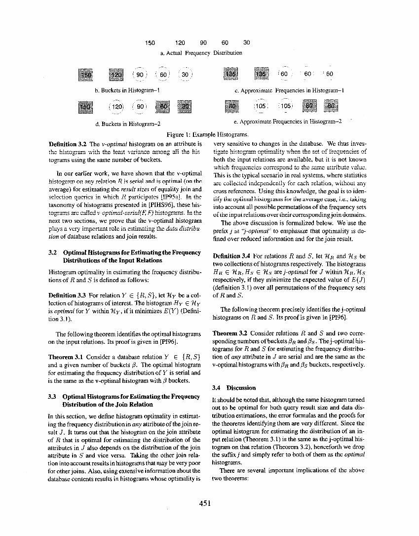
The example in Figure 1 illustrates the above by listing two different histograms on an attribute of relation with two buckets in each. The frequencies of all the attribute values are listed in Figure 1 a. Figures 1 b and 1 d show the grouping of frequencies into buckets for the two histograms. Figures lc and le show the resulting approximate frequencies.

Next we define a class of histograms that is important to the problem at hand.

Definition 2.1 [Ioa93] A histogram for attribute 0 of a relation is serial, if for all pairs of buckets 61, ba, either tldk E bl, dl E ba, the inequality f(dk) 2 f(dl) holds, or Vdk E bl, dl E bz, the inequality f(dk) < f(dl) holds.

Note that the buckets of a serial histogram group frequencies that are close to each other with no interleaving. For example, in Figure 1, Histogram- 1 is a serial histogram while Histogram-2 is not. This is in contrast to the traditional equi-width and equi-deprh histograms which group contiguous ranges of attribute values into buckets.

A histogram bucket whose domain values are associated with equal frequencies is called univalued. Otherwise, it is called multivalued. Univalued buckets characterize the following important classes of histograms. Definition 2.2 [Ioa93] A histogram with p - 1 univalued buckets and one multivalued bucket is called biased. If

1 We often denote the frequency simply as f (dk ) when the name of the relation is clear from the context.

these univalued buckets correspond to the domain values with the p - 1 highest and lowest frequencies, then it is called end-biased.

Note that end-biased histograms are serial.

3 Histogram Optimality

Let R and S be two relations participating in the equi-join on attribute cr, and J be the resulting relation. We estimate the data distributionof & in J from the histograms on R and sas:

f;(d) = fkb-4 x f;(d).

where, J$ (d) is the approximate frequency of d in relation X, obtained from a histogram.

An important issue to be addressed is the accuracy of these estimations. For this purpose, we first define the error incurred in using an approximate frequency distribution. The following metric is a standard measure of the deviation between two distributions.

Definition 3.1 The error of a histogram in approximating the frequency distribution of an attribute (Y of relation X is defined as the squared deviation of the actual and approximate distributionsover all the attribute values in the domain V of o, i.e,

E(X) = ~(fx(d) - fkW2.

Since the number of histogram buckets is determined by the available catalog space, accuracy depends only on how the domain values are grouped into buckets in the two histograms. In the next few sections, we present the results identifying the optimal histograms on the input relations R and S, which minimize the errors in estimating the frequency distributions of R, S, and the join result J.

3.1 V-optimal histograms

In this section, we characterize an important class of histograms, which are relevant to our optimality results. First some useful notation:

bi The i-th bucket in the histogram, 1 5 i 2 p (numbering is in no particular order).

Pi The number of frequencies in bucket bi.

x The variance of the frequencies in bucket bi .2

Define the variance of a histogram to be

Y=&pjv,. i=l

(1)

2v, = c , dE6 (f(4--d2 Pi

, ai is the average of frequencies in b,.

450

150 120 90 60 30

a. Actual Frequency Distribution

b. Buckets in Histogram-l

i 12i) (90 i -* -*

d. Buckets in Histogram-2

c. Approximate Frequencies in Histogram-l _- -

(,105 I 1105i -

f$g&j

e. Approximate Frequencies in Histogram-2 .

Figure 1: Example Histograms.

Definition 3.2 The v-optimal histogram on an attribute is the histogram with the least variance among all the histograms using the same number of buckets.

In our earlier work, we have shown that the v-optimal histogram on any relation R is serial and is optimal (on the average) for estimating the result sizes of equality join and selection queries in which R participates [IP95a]. In the taxonomy of histograms presented in [PIHS96], these histograms are called v-optimal-serial(~ F) histograms. In the next two sections, we prove that the v-optimal histogram plays a very important role in estimating the data distribution of database relations and join results.

3.2 Optimal Histograms for Estimating the Frequency Distributions of the Input Relations

Histogram optimality in estimating the frequency distributions of R and S is defined as follows:

Definition 3.3 For relation Y E {R, S}, let 31~ be a col- lection of histograms of interest. The histogramHy E 3cy is optimal for Y within 31y, if it minimizes E(Y) (Defini- tion 3.1).

The following theorem identifies the optimal histograms on the input relations. Its proof is given in [P196].

Theorem 3.1 Consider a database relation Y E {R, S} and a given number of buckets /3. The optimal histogram for estimating the frequency distribution of Y is serial and is the same as the v-optimal histogram with /3 buckets.

3.3 Optimal Histograms for Estimating the Frequency Distribution of the Join Relation

In this section, we define histogram optimality in estimating the frequency distribution in any attribute of the join result J. It turns out that the histogram on the join attribute of R that is optimal for estimating the distribution of the attributes in J also depends on the distribution of the join attribute in S and vice versa. Taking the other join relation into account results in histograms that may be very poor for other joins. Also, using extensive information about the database contents results in histograms whose optimality is

very sensitive to changes in the database. We thus inves- tigate histogram optimality when the set of frequencies of both the input relations are available, but it is not known which frequencies correspond to the same attribute value. This is the typical scenario in real systems, where statistics are collected independently for each relation, without any cross references. Using this knowledge, the goal is to identify the optimal histograms for the average case, i.e., taking into account all possible permutations of the frequency sets of the input relations over their corresponding join domains.

The above discussion is formalized below. We ‘use the prefix j in “j-optimal” to emphasize that optimality is defined over reduced information and for the join result.

Definition 3.4 For relations R and S, let %R and 7i.s be two collections of histograms respectively. The histograms HR E ‘h!~, Hs E 31s are j-optimal for J within %~,‘?ts respectively, if they minimize the expected value of E(J) (definition 3.1) over all permutations of the frequency sets of R and S.

The following theorem precisely identifies the j-optimal histograms on R and S. Its proof is given in [PI96].

Theorem 3.2 Consider relations R and S and two corresponding numbers of buckets PR and p.s. The j-optimal histograms for R and S for estimating the frequency distribution of any attribute in J are serial and are the same as the v-optimal histograms with /!IR and ps buckets, respectively.

3.4 Discussion

It should be noted that, although the same histogram turned out to be optimal for both query result size and data distribution estimations, the error formulas and the proofs for the theorems identifying them are very different. Since the optimal histogram for estimating the distribution of an input relation (Theorem 3.1) is the same as the j-optimal histogram on that relation (Theorem 3.2), henceforth we drop the suffixj and simply refer to both of them as the optimal histograms.

There are several important implications of the above two theorems:

451

1. A single precomputed histogram on each input relation is sufficient for estimating the data distributions of the input as well as the result relations most accurately.

2. The optimal histogram on R is independent of S and vice versa. Each can therefore be identified by focus- ing on the frequency set of that relation alone. This histogram will be optimal for any query where the relation is joined on the same attribute with any relation of any contents.

3. Since the optimal histogram on a relation is the same as the v-optimal histogram, algorithms for identifying the latter can be applied to precisely identify the optimal histogram for result distribution estimation. This is also very significant in practice because the same histograms can be used for multiple purposes.

4 Construction, Storage, and Effectiveness of Optimal Histograms

In this section, we deal with the efficiency of construction and maintenance of optimal serial and end-biased histograms. Algorithms for constructing both these histograms require computing the frequency distributionof the attribute, which involves a scan of the relation and exces- sive CPU costs. In practice, the desired frequencies can be estimated quite accurately from a small random sample (ti 2000 tuples) obtained using reservoir sampling [Vit85]. The estimated frequency of a value di is simply niN/n, where ni is the number of tuples in the sample with attribute value di, n and N are the total number of tuples in the sample and the relation respectively.

4.1 Serial Histograms

Construction (Algorifhm OptHist)[IP95a]: The algorithm identifies the optimal serial histogram with ,L3 buckets on a relation R as follows. The frequency set of R is sorted and then partitioned into /3 contiguous sets in all possible ways. Each partitioning corresponds to a unique serial histogram with the contiguous sets as its buckets. The error corresponding to each histogram is computed using definition 3.1 and the histogram with the minimum error is returned as optimal. In our earlier work we had shown that this.algorithm is exponential in /? [IP95a].

Storage and Maintenance: Since there is usually no order-correlation between attribute values and their frequencies, for each bucket in the histogram we need to store the average of the frequencies in it and a list of the attribute values mapped to the bucket. Clearly, for a high cardinality attribute, this structure requires too much space. By storing the boundaries of buckets instead of the entire set of values, the space requirements become easily manageable, at the expense of losing optimality.

4.2 End-Biased Histograms

In our earlier work [Ioa93], we have proved that the v- optimal biased histogram for a relation R is end-biased. End-biased histograms are important in practice because they are inexpensive to compute and maintain as we show below.

Construction (Algorihn OptBiasHist)[IP95a]: The algorithm works by enumerating all possible end-biased histograms on the chosen attribute and picking one with the least variance (Definition 3.1). They can be efficiently generated by using a heap tree to pick the highest and lowest p - 1 frequencies and enumerating the combinations of placing them in univalued buckets. Fortunately, the number of end-biased histograms is approximately equal to the number of buckets ,0. It can be shown that, given the fre-. quency set B of a relation R and an integer ,0 > 1, this algorithm finds the optimal end-biased histogram with ,0 buckets in O(M+(P- 1)ZogM) time, where A4 is thecardinality ofB.

Storageand Maintenance: In order to store an end- biased histogram, all the univalued buckets (<domain value, frequency> pairs) need to be stored in some catalog structure. By assuming that all other domain values fall in the multi-valued bucket, we only need to store the frequency corresponding to the multi-valued bucket in the catalog. Since the number of buckets tends to be quite small in practice (5 20), the space requirement is small and sequen- tial search of the buckets will be sufficient to access the information efficiently.

4.3 Database Updates After any update to a relation, the corresponding histogram may need to be updated as well. Delaying the propagation of database updates to the histogram, which is the usual approach taken by systems, can introduce errors. We are currently studying appropriate schedules of database update propagation. Any proposals in that direction do not affect the results presented here, so this issue is not discussed any further.

4.4 Comparison of Costs The above algorithms were implemented on a SUN-SPARC workstation with a 10 MIPS CPU and their execution times were observed for varying cardinalities of frequency sets and numbers of buckets. Table 1 illustrates the difference in construction costs between the two algorithms. It does not include the cost for obtaining the frequencies. For end- biased histograms, the numbers presented are for p = 10 buckets, and are very similar to what was observed for /3 ranging between 3 and 200. The times increase drastically for the algorithms for the optimal serial histograms. We did not compute the remaining entries for the serial histograms because that would take take too much time and the results obtained already convey the construction cost differences between the two histograms.

452

z=l , M=lOO (Result Size = 60760)

. _ --- 5000 v +- * ‘.“,, _ --._ + ..____ _.--

5 5 4000- z E ‘Z 3000 - ‘5 d E d 2000-

5 * lOOO-

Uniform Equi-Width

Equi-Height End-S:;;:

04 0 5 10 Num&Tof bu%ts 25 30 35 0.5 1 1.5 2 2.5 3 3.5 4 4.5 5

(b) Zipf skew (z)

Figure 2: d as a function of the number of buckets. Figure 3: u as a function of skew (z parameter of Zipf).

5 Parallel Joins

Table 1: Construction cost for optimal serial and end-biased histograms

Time taken (XX) Number of Serial 1 End-biased

attribute values P=Sl p=51 B= 10

4.5 Effectiveness of Optimal Histograms in Result- Distribution Estimation

We studied the performance of various histograms with varying number of buckets and skew in the data. We used five types of histograms: trivial, optimal serial, optimal end-biased, equi-width and equi-depth histograms, with the number of buckets p ranging from 1 to 30. The trivial histogram is the usual uniform distribution assumption over the entire column,. In an equi-width histogram, the number of attribute values associated with each bucket is the same; in an equi-depth (or equi-height) histogram, the total number of tuples having the attribute values associated with each bucket is the same. The frequency sets of the relations follow the Zipf distribution, since it presumably reflects reality [Chr84, Zip49]. Its t parameter takes values in the range [0 - 51, which allows experimentation with varying degrees of skew and the number of frequencies (M) was kept at 100. Figures 2 and 3 show the square root of variance (Eq. 1) generated by the five types of histograms as ,B and z are varied respectively [IP95a]. In almost all cases, the histograms can be ranked in the following order from lowest to highest error: optimal serial, optimal end- biased, equi-depth, equi-width, and trivial (uniformity assumption). We can see that the serial and end-biased histograms handle all levels of skew quite satisfactorily and increasing the number of buckets beyond a point adds little to their accuracies.

2oooc

b b 15OOa

‘ii s ‘Z 2 10000 9” E $ 5 5000 cn

M=lOO, Number of buckets=5

Uniform - Equi-Width -+----

Equi-Height -‘EL End-Biased I-

Serial -.A-.-.

I-

l-

I-

‘k. ‘..,

‘.., ‘...

‘h. ‘.,.

‘._, “R,,

.._, ‘.__

Q...,.

1

In the remainder of the paper, we study an application of our optimality results to load balancing during parallel Hybrid hash joins. We assume a shared-nothing environment con- sisting of several nodes connected by a fast network, similar to the Gamma system [DGG+86]. Each node consists of a single CPU with reasonably large memory and two disks attached to it. All relations are assumed to be partitioned across all the disks. The exact partitioning algorithm used is not relevant to our discussion below. More details about the Gamma system can be.found elsewhere [DGG+86].

5.1 Description of Parallel Hybrid Hash Join Algo- rithm (P%‘?L~O~JV)

In this section we describe a typical parallel execution of the Hybrid hash join algorithm [DGS+90]. In the rest of the paper, R and S denote the build and probe relations, respectively. Usually, the smaller relation is chosen as the build relation. Some of important steps in the algorithm are listed below. We omit some issues such as hash bucket overflows in this discussion.

1. Split Table Computation: The split table contains mappings of attribute values to nodes, which are used in distributing the tuples below. In Gamma, its computation is a trivial step, involving mapping the attribute values to various nodes using a hash function. In general, this step may involve more complicated load- balancing algorithms (to be discussed later). Next, all the processors execute the following steps:

2. Redistribution: Scan R and S in succession from the local disk and use the split table to direct the tuples to the nodes.

3. Build: As the R tuples are being received, build a hash table using a hash function h. The number of hash buckets is determined from the amount of available

453

memory and the size of R [Sha86]. The first bucket is retained in memory, while others are stored on disk.

4. Probe: As the S tuples are being received, hash them using h. If they map to the first hash bucket, they are joined with the tuples from the first hash bucket of h!. Otherwise, they are stored in the corresponding hash bucket of S on disk. After all the S tuples have been received, corresponding hash buckets of R and S are read from the disk and their tuples are joined.

5. Postprocess: The tuples resulting from joining the input relations in the previous step are possibly redistributed across the nodes using another split table, either to be stored on disk or to participate in the next operator in the query.

Next, we present various kinds of skew that affect the performance of QU’K?c?Z~/.

5.2 Data Skew

Like most parallel operations in a shared-nothing environment, parallel hash joins also perform poorly under data skew. Data skew can lead to imbalances’in the number of tuples processed by each node. This causes problems in re- alizing high performance because the total runtime of a parallel algorithm is determined by the busiest node. We describe the two most important kinds of skew identified in the literature [WDJ91], which cause load imbalances during join execution.

1. Attribute Value Skew (AVS): It arises due to non- uniform data distributions in the join attribute in the input relations. It may result in biased distributions of data among the nodes when the split table maps values to nodes without taking their frequencies into account. This causes different workloads across nodes during join processing, bucket overflows when nodes are allocated very large hash buckets, and network hot spots because few of the nodes may receive a large number of tuples.

2. Join Product Skew (JPS): It arises due to differences in the join selectivities of data processed by different nodes. It can occur even if R and S have no AVS and is one of the subtler kinds of skew to detect. It mainly affects the postproces.s phase of join execution, by requiring a node with large output to do more work distributing the result tuples.

5.3 Cost Model

The goal of a load-balancing algorithm is to equalize load (the amount of CPU and I/O work) done by various nodes participating in the parallel execution. In this section, we

’ develop a numerical measure to capture the effects of AVS and JPS on the load on each node duringQ‘MgC32N. We

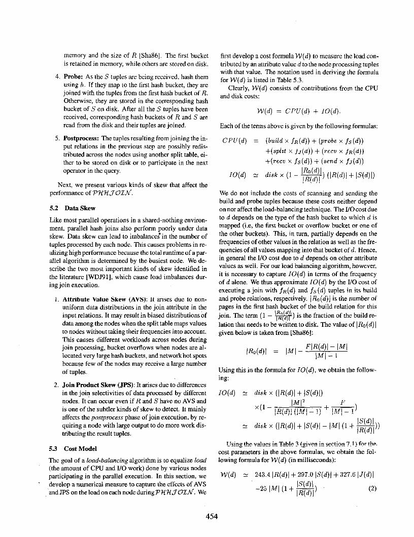
first develop a cost formula W(d) to measure the load con- tributed by an attribute value d to the node processing tuples with that value. The notation used in deriving the formula for W(d) is listed in Table 5.3.

Clearly, W(d) consists of contributions from the CPU and disk costs:

W(d) = CPU(d) + IO(d).

Each of the terms above is given by the following formulas:

CPU(d) = (build x fR(d)) + (probe x fs(d))

+(s$it x fJ(d)) + (mcv x fR(d)) +(recv x fs(d)) + (send x fJ(d))

IW4l IO(d) 2: disk x (1 - - JR(d), ) (‘R(d)’ + ‘S(d)‘)

We do not include the costs of scanning and sending the build and probe tuples because these costs neither depend on nor affect the load-balancing technique. The I/O cost due to d depends on the type of the hash bucket to which d is mapped (i.e, the first bucket or overflow bucket or one of the other buckets). This, in turn, partially depends on the frequencies of other values in the relation as well as the frequencies of all values mapping into that bucket of d. Hence, in general the I/O cost due to d depends on other attribute values as well. For our load balancing algorithm, however, it is necessary to capture IO(d) in terms of the frequency of d alone. We thus approximate IO(d) by the I/O cost of executing a join with fR(d) and fs (d) tuples in its build and probe relations, respectively. 1 Ro(d) 1 is the number of pages in the first hash bucket of the build relation for this join. The term (1 - l/$$$) is the fraction of the build relation that needs to be written to disk. The value of (Ro (d) 1 given below is taken from [Sha86]:

IRo( = IMI - “T$rl’“’

Using this in the formula for IO(d), we obtain the following:

IO(d) 21 disk x ([R(d)1 + IS(d

WI2 ‘(’ - IR(d)l (IMI - 1) + ,Mr- 1)

= disk x (IWI + IS( - lMl (I+ ,R(d), IS( ))

Using the values in Table 3 (given in section 7.1) for the. cost parameters in the above formulas, we obtain the following formula for W(d) (in milliseconds):

W(d) N 243.4 [R(d)1 + 297.0 IS(d)( + 327.6 jJ(d)l

IS(d) I -25 i”i ci + lR(d)l) (2)

454

J fx (4 IV) I

PI F

build probe split send recv disk

Table 2: Description of terms used in the cost model Result of joining relations R and S Frequency of d in relation X, X E {R, S, J} Number of pages necessary to hold the tuples with value d in relation X (i.e., IX(d) ( Number of main memory pages “Fudge factor” to take into account space overheads of a hash table (2 1.4) [Sha86] Cost of inserting a tuple in the build hash table Cost of probing the hash table for a single tuple Cost of hashing a tuple using a split table Cost of writing a tuple into the output buffer Cost of reading a tuple from the input buffer Disk I/O cost for a page after the redistribution phase

The load on a node is simply the sum of the costs W(d) of all the values d mapped to that node by the split table, where W(d) is computed using (2). Note that, despite our attempts to choose a reasonable model for the execution environment, the parameter values in the cost formula (or the cost formula itself) may be different in any given real system. In that case, the cost formula must be approppriately updated.

5.4 Histogram Optimality in Load Balancing

In section 5.3, we introduced thecost formula for W, which depends only on the frequency distributions of the join attribute Q in the two input relations R, S and in thejoin result J. We have developed a load balancing algorithm, called ‘HZS’H, that makes use of this formula in creating a split table, so that the loads on all the nodes in the system are approximately equal, thus achieving load balancing. In order to estimate the cost formula most accurately, we need reasonably accurate approximations of these three data distributions. This is precisely what we achieved in Theorems 3.1 and 3.2, which show that the v-optimal histograms constructed on rr in R and S identify the data distribution of a in R, S, and J most optimally. Next, we present describe our algorithm for load balancing.

5.5 Histogram-Based Algorithm for Skew Handling (%ZS31)

Let HA and Hg be the optimal histograms on the join attribute of two input relations A and B, respectively, precomputed using algorithm OptBiasHist (section 4). The first phase of ‘liZS’?i below analyzes the input relations to make some important decisions for join execution3. The second phase computes the split table for load balancing. Some of the techniques presented in the second phase were originally proposed by Dewitt et al. in [DNSS92].

Analysis Phase: The histograms HA and HB are ana- lyzed to detect the levels of AVS in the input relations. We

3 In practice, this step will be performed by the optimizer w~hile choosing the optimal query plan.

use the variance of the frequencies in the approximate distributions as a measure of skew. Next, the build and probe relations are chosen from A and B for the best join performance. Let A be the smaller relation. If the level of skew in both the relations is very small, exit from this algorithm and execute P?i?tJOZN without load balancing, with A as the build relation R and B as the probe relation S. If A is much smaller than B or fits in memory, choose A as the build relation R and B as the probe relation S. Otherwise, choose the relation with the highest skew as the probe rela- . tion S and the other relation as the build relation R. This choice is justified in our experiments (Section 7.4).

Partition Phase: The cost formula W (Eq. 2) is eval- uated for the attribute values in the histograms using their frequencies from the approximate frequency distributions of R, S and J. Next, the attribute values are divided into a fixed number of partitions, which are assigned to the nodes in a round robin scheme, such that the sum of W over all values in the partitions are approximately equal. Values not occurring in the histogram are assumed to be mapped to the nodes using a static hash function, similar to Gamma. In order to avoid large hash buckets that arise when the same value occurs with very high frequency, an attribute value may be mapped to multiple nodes [DNSS92]. In this case, the fraction of W(d) assigned to each node is also recorded in the split table. During the redistribution phase of thejoin, tuples from one of the relations having’d in their join attribute are sent to various nodes in proportion of these frac- tions. For correctness all the tuples from the other relation with this attribute value should be sent to each such node (i.e., multicast), incurring some additional overhead. In our algorithm, tuples from the relation with the smaller frequency of d are multicast in order to minimize the number of tuples processed. The results of our experiments on handling skew in the probe relations (section 7.4) justify this decision.

The number of partitions is chosen as k x v, where k is the number of nodes and v is the fixed number of virtual

455

processors per node [DNSS92]. The number 21 is chosen so that there are small partitions and an attribute value d occurring with high frequency is mapped to multiple partitions.

5.51 cost of 312sx

Since the histograms on the base relations are usually precomputed, their construction does not add to the cost of XZS7i which is run at join execution time. %!cZSX incurs no additional I/OS other than reading the small histogram structures from the catalogs, which are usually present in main memory. The CPU costs during the two phases are also negligible because the number of buckets in the histograms is very small (typically 20). The only significant cost is incurred during join processing because some of the attribute values may be mapped to multiple nodes, thus increasing the size of the split tables and hence the search time. But, our results show that this cost is insignificant compared to the savings in the execution time overhead from load balancing.

6 Earlier Approaches to Load Balancing

Most of the earlier approaches can be classified into two cat- egories - Conventional and Sampling-Based. Based on earlier analyses of these algorithms [HY95] and our own studies, we have identified the best proposed solutions in both classes. Their split table computation phases are described below.

6.1 Conventional : Extended Adaptive Load Balanc- ing Parallel Hash Join (ABP)

This algorithm was proposed in [HL91]. Each node scans and partitions its local portion of build relation into hash buckets and stores them back on the disk. All nodes report the sizes of their portions of the hash buckets to a pre- designated coordinator. The coordinator creates a split table by mapping the hash buckets to the nodes so that approximately the same number of tuples are allocated to each node.

This approach incurs an additional read and write of the relation if the local partitions of relations do not fit in memory. Also, since alltuples with the same attribute value are sent to a single node, some nodes may end up with a very large hash bucket in case of skewed distributions and the algorithm fails to balance load. Finally, the algorithm ignores AVS of the probe relation and JPS.

6.2 Sampling-Based : Virtual Processor Partitioning WPP)

This algorithm was proposed in [DNSS92]. A small sample of the relations is collected and the relation with the highest skew is chosen as the build relation. The sampled attribute values are sorted and partitioned into (k x v) equal sized partitions, where k is the number of nodes and w is a fixed

number of virtualprocessors per node. These partitions are assigned to the nodes using a simple round robin scheme, resulting in a split table.

Compared to d&7+, this approach replaces a complete scan of the relations by an inexpensive sampling phase. Like %ZS’?t, this algorithm also maps a frequent value to multiple nodes, thus handling AVS better than d&T'+. But, this algorithm ignores AVS in the probe relation (once the build and probe relations are chosen) and JPS. Also, page level sampling can introduce errors when the tuples in a page are correlated on the join attribute, e.g, when the relation is clustered on that attribute.

7 Experiments

In this section, we study the performance of the four load balancing algorithms: BASIC (no load balancing), dBJ+, VPP, and 3cZS31, under various inputs and system parameters.

7.1 Execution Environment

All our experiments were conducted on a simulator for the Gamma parallel database system. The basic simulator was written in the CSIM/C++ process-oriented machine lan- guage and accurately captures the algorithms and costs of Gamma [Bro94]. The simulator assumes uniform data, so its use of split tables is trivial. Hence, we enhanced it with the capability to operate on non-uniform data and to use a split table computed by the load balancing algorithms. We describe some relevant parts of the simulator below.

Query Processing: The query is submitted by a simulated terminal to the scheduler process. A thread is created for every simulated node for each operator to be executed. The scheduler sets up communication channels with these threads and broadcasts the split table and the operator to be executed. Each thread executes the operator on the tuples from a simulated disk corresponding to its node. Resulting tuples are redistributed using the split table. This process is repeated for every operator in the query plan.

Hardware Environment: The simulator models la- tency in the interconnection network but assumes a very large bandwidth. This is in agreement with most real systems (iPSC/2 Hypercube, CM-5, Paragon). Communica- tion between threads is in units of 8 KByte messages. The disk is modeled based on the Fujitsu Model M2266 (1 GB, 5.25”) disk drive. The CPU is scheduled using a round- robin policy and the page replacement in the buffer pool is based on LRU with love/hate [Ht90] hints. The instruction counts for various operations in the validated simulator are taken from [SN93] and are listed in Table 3.

7.2 Experiment Testbed

Algorithms: The following algorithms are used to compute the split table in ‘P’?KU~c1Z~. All the experiments compute the time taken by PW?L?OZN using the split table

456

CPU Cost Parameter Table 3: Simulation Parameter Settings

] No. Instr. )I Configuration/NodeParameter 1 Value

____ _- r-- ----- - -- I--- ------ , ___ - ____ __-_- ___.. ___.. - _ -.--. --.I--

Probe Hash Table 200 I] Disk Settle Time 2.0 msec Insert Tuple in Hash Table I

I 100 11 Disk Transfer Rate

II --~~ ----~~---~ 3.09 MB/set

HashTuple ~_ I usine Solit Table 1 I 500 II Disk CacheC II ~~~~ ontext Size 4 pages ADOIV a Predicate 100 11 Disk Cache Size 8 contexts

I. .

Copy 8K Message to Memory Message Protocol Costs

10000 Disk Cylinder Size 1000 Sampling Overhead

83 pages 0.6 set

resulting from these schemes, including the time taken by of unique values was chosen, up to 1 million, depending on the split table computation step. the skew such that the lowest frequency equals 1.

l BdSZC: No load balancing. For this algorithm, we obtained the split table by mapping equal number of attribute values to the nodes.

7.3 Effect of Virtual Processors on the Performance of ?-US31

l d&7+: Extended adaptive load balancing (section 6.1).

l VPP: Sampling-based virtual processor partitioning (section 6.2). The number of virtual processors per node was fixed at 60 as recommended in [DNSS92]. Sample size was fixed at 14400 tuples.

l 7iZS’X: Histogram-based skew handling (section 5.5). In order to study the effects of AVS in the probe relation, the Analysis Phase of ‘liZS%! was not executed in any of the experiments. All experiments were conducted using the optimal end-biased histograms obtained from a sample of 14400 tuples from the data. The number of buckets in the histogram was fixed at 20, because accuracy is not very sensitive to the number of buckets beyond this. The number of virtual processors per node was varied from 1 to 100 in the first experiment (section 7.3) and fixed at a single value of 60 for all the subsequent experiments.

In section 5.5, we briefly described the role of the number of virtual processors (v) in ‘l-lZS%. While higher values of w ensure that a value with high frequency is mapped to multiple nodes, they also incur overheads due to multicasting tuples to many nodes. We conducted experiments to measure this trade-off in terms of the time taken for join execution for different values of 21 ranging from 1 to 100. Build relation’s skew was varied from z = 0 to 2 = 5 and probe relation was chosen to be uniform. Based on the results we decided to use n = 60 for all our remaining experiments [PI96]. The same value was arrived at in [DNSS92] also.

Resources: The number of nodes participating in the join was fixed at 16, except for the speed-up experiments. Scheduling and other administrative operations were run on a separate node. Values of other resources are given in Ta- ble 3.

7.4 Effect of Attribute Value Skew

The first experiment studies the effect of AVS in the build relation’s join attribute. The skew is varied from t = 0 to ,z = 5. The probe relation is chosen to have a uniform distribution. The results are plotted in Figure 4. It can be seen that as skew increases, dBJ’+ fails to balance load, because it does not distribute the large join buckets containing the most frequent values. On the other hand, both ?lZS’Jf and YPP handle AVS in the build relation satisfactorily because they split these large hash buckets.

m: All the input relations consisted of 220 (approximately 1 million) tuples of 100 bytes each. Frequencies of the join attribute values are taken from the Zipf distribution [Zip49, Chr84]. Skew is modeled by varying the z parameter of the Zipf distribution from 0 to 5. The number

The second experiment studies the effect of AVS in the probe relation, while the build relation is chosen to be uniform, and the results are plotted in Figure 5. For this case, V’PP will choose the skewed relation as the build relation and have the same performance as in the previous experiment. For comparison purposes, we are including the result of running YPP by forcing it to use the skewed relation as the probe relation. We call this modified algorithm VPP’. d&7+ performs the worst because it totally ig-

451

2500 , A

2000 -

g 1500.

2 I= .c lOOO- 4

~ BASIC + , ABJ+ .d....

VPP --a- HISH -*---

0 1 2 3 4 5 skew (z)

Figure 4: Effect of Build Relation Skew.

nores the skew in the probe relation. It is clear that 31ZSX almost completely eliminates the effect of probe relation’s skew on join performance, because it distributesvalues with high frequency in the probe relation across multiple nodes. Note that all algorithms perform significantly better than in the previous experiment, justifying our decision to use the most skewed relation as the probe relation. 7.5 Effect of join product skew

In this experiment, we restricted the attribute value skews of both the build and probe relations to be very small (0 - 0.8). Even these low AVS values can still result in significant JPS. The performance results shown in Figure 6 demon- strate that ?&!GJf achieves significantly better load balancing. This is because its cost formula W takes JPS into account, while other schemes fail to detect it.

8 50000-

.E 40000 - I-

5 3OOoo-

20000 -

10000-I / ,A ,’ 0 __

0 0.2 0.4 0.6 0.8 1 skew (z)

Figure 6: Effect of Join Product Skew.

7.6 Speed-up Performance

Load imbalances have significant adverse effects on the speed-up of a parallel system. Hence, we studied the behav- ior of various load balancing algorithms as system configuration is varied. To study speed-up, the number of nodes was varied from 1 to 19. Data in both the inputrelations was moderately skewed (.z = 0.6). The join costs for various

220- BASIC * ABJ+ -+---

200- vpp’ ..B... 180- HISH -*

160-

140-

-I 0 1 2

eke: (z) 4 5 6

Figure 5: Eflect of Probe Relation Skew.

algorithms are plotted in Figure 7. The curve IDEAL corresponds to a hypothetical algorithm with linear speed-ups and is included for comparison purposes. It is clear that all the load balancing algorithms (d&7+, VPP, and ‘KZS%) have very good speed-ups, with 312831 having almost linear speed-up. Referring back to Figure 6, it becomes clear that for higher skews 31ZS31 will perform much better than the other two algorithms. -

5OGQ r

4500 -

4000-

3500-

3 3000.

E 2500 - I= .c 2OOQ- 3

1500-

iooo-

BASIC - ABJ+ ---- “pp ..o.... HISH -n --

IDEAL ----

5 10 15 Number of Nodes

Figure 7: Speed-Up Performance.

8 Conclusions

Estimation of result distributions plays an important role in several components of a DBMS. Using precomputed histograms is a feasible technique in practical systems. A major result of the paper is that the same histograms on database relations are optimal for estimating the distribution of those relations as well as the results of equi-joins, and are independent of all other relations in the database. These histograms were also shown earlier to be optimal for join selectivity estimation, thus establishing their universality. As a special application, we also developed an efficient solution for load balancing in parallel DBMSs by handling all kinds of skew in the data. We derived a cost for-

458

mula for the load on a machine which captures the effects of various kinds of skew. We presented a load balancing algorithm which uses histograms on the base relations to estimate the cost formula and balances the load across all the nodes. Experimental comparison with the current state- of-the-art approaches demonstrated that our algorithm balances load most effectively under all levels and kinds of skew. Acknowledgements: The idea of using optimal histograms in the context of load-balancing was suggested to us by Sridhar Chandrasekharan. The authors are also grateful to Minos Garofalakis, Joe Hellerstein, Navin Kabra, and Dha- rani Nandakuru for carefully reviewing the paper, and to Prof. David Dewitt for correcting some of our citations to work in parallel databases.

References [B+ 901

[Bro94]

[Chr84]

[DGG+ 861

[DGS+ 901

[DNSS92]

[H+90]

[HL91]

[HY95]

[IC91]

[Ioa93]

H. Boral et al. Prototyping Bubba: A highly parallel database system. IEEE Knowl. Data Engineering, 2(l), March 1990. Kurt Brown. Zetasim user’s guide. Unpublished Manuscript, Univ of Wisconsin, Madison, 1994. S. Christodoulakis. Implications of certain assump- tions in database performance evaluation. ACM TODS, 9(2): 163-186, June 1984. David J. Dewitt, R. H. Gerber, Goetz Graefe, M. L. Heytens, K. B. Humar, and M. Mu- ralikrishna. GAMMA - a high performance dataflow database machine. Proc. of the 12th Int. Conf: on Very Large Databases, August 1986. David J. Dewitt, S. Ghandeharizadeh, D. A. Schnei- der, A. Bricker, H. I. Hsiao, and R. Rasmussen. The Gamma database machine project. IEEE Trans. on Knowledge and Data Eniineering, 2(l), 1990. .

David J. Dewitt, J. F. Naughton, D. A. Schneider,and S. Seshadri. Practical skew handling in parallel joins. Proc. of the 18th Int. Cor$ on Very Large Databases, August 1992. Laura Haas et al. Starburst mid-flight: As the dust clears. IEEE Trans. Knowledge Data Eng., 2(l), 1990. Kien A. Hua and Chiang Lee. Handling data skew in multiprocessor database computers using partition tuning. Proc. of the 17th Int. Conj on Very Large Databases, September 199 1. Kien A. Hua and Honesty C. Young. A performance evaluation of load balancing techniques for join operations on multicomputer database systems. Proc. of IEEE Con$ on Data Engineering, 1995. Yannis Ioannidis and Stavros Christodoulakis. On the propagation of errors in the size of join results. Proc. of ACM SIGMOD ConA pages 268-277,199l. Yannis Ioannidis. Universality of serial histograms. Proc. of the 19th Int. Con5 on Very Large Databases, pages 256-267, December 1993.

[IP95a]

[IP95b]

[K090]

[LY88]

[MD881

[PI961

[PIHS96]

[PSC84]

[SD891

[Sha86]

[SN93]

[St0861

[Vit85]

[WDJ91]

[Zip491

Yannis Ioannidis and Viswanath Poosala. Balancing histogram optimality and practicality for query result size estimation. Proc. of ACM SIGMOD Conf, pages 233-244, May 1995.

Yannis Ioannidis and Viswanath Poosala. Histogram- based solutions to diverse database estimationprob- lems. IEEE Data Engineering Bulletin, 18(3):10-18, December 1995.

Masaru Kitsueregawa and Yasushi Ogawa. Bucket spreading parallel hash: A new, robust, parallel hash join method for data skew in the super databasecom- puter (SDC). Proc. of the 16th Int. Cons on Very Large Databases, 1990.

S. Lakshmi and P. S. Yu. Effect of skew on join performance in parallel architectures. Proc. of In- ternational Symp. on Databases in Parallel and Dis- tributed Systems, December 1988.

M. Muralikrishna and David J Dewitt. Equi- depth histograms for estimating selectivity factors for multi-dimensional queries. Proc. of ACM SIGMOD Conf, pages 28-36,1988.

Viswanath Poosala and Yannis Ioannidis. Estima- tion of query-result distribution and its application in parallel-join load balancing. Unpublished technical report, University of Wisconsin-Madison, July 1996.

Viswanath Poosala, Yannis Ioannidis, Peter Haas, and Eugene Shekita. Improved histograms for selectivity estimation of range predicates. Proc. of ACM SIGMOD Con$ pages 294-305, June 1996.

Gregory Piatetsky-Shapiro and Charles Connell. Ac- curate estimation of the number of tuples satisfying a condition. Proc. of ACM SIGMOD Conf, pages 256- 276,1984.

Donovan A. Schneider and David J. Dewitt. A performance evaluation of four parallel join algo- rtihms in a shared-nothing multiprocessor environment. Proc. ofACMSIGMOD Conf, June 1989.

Leonard D. Shapiro. Join processing in database systems with large main memories. ACM Transac- tions on Database Systems, 11(3):239-264, Septem- ber 1986.

Ambuj Shatdal and Jeffrey F. Naughton. Using shared virtual memory for parallel join processing. Proc. of ACM SIGMOD ConJ May 1993.

Michael Stonebraker. The case for shared nothing. Database Engineering, 9(l), 1986.

J. S. Vitter. Random sampling with a reservoir. ACM Trans. Math. Sojware, 11:37-57,1985.

C. B. Walton, A. G. Dale, and R. M. Jenevin. A taxonomy and performance model of data skew effects in parallel joins. Proc. of the 17th Int. Con5 on Very Large Databases, April 199 1.

G. K. Zipf. Human behaviour and the principle of least effort. Addison-Wesley, Reading, MA, 1949.

459

estimation of query-result distribution and its

Documents