query estimation techniques in database systems
TRANSCRIPT

Query Estimation Techniques in Database Systems
Dissertation
zur Erlangung des Grades
Doktor der Ingenieurwissenschaften (Dr.-Ing.)
der Naturwissenschaftlich-Technischen Fakultat I
der Universitat des Saarlandes
von
Diplom-Informatiker
Arnd Christian Konig
Saarbrucken,
im Dezember 2001
brought to you by COREView metadata, citation and similar papers at core.ac.uk
provided by Acronym


Contents
1 Introduction 11.1 Motivation . . . . . . . . . . . . . . . . . . . . . . . . . . . . . . . . . . . . . . . 11.2 Problem Description . . . . . . . . . . . . . . . . . . . . . . . . . . . . . . . . . . 3
1.2.1 Synopsis Construction . . . . . . . . . . . . . . . . . . . . . . . . . . . . . 41.2.2 Physical Design Problem for Data Synopses . . . . . . . . . . . . . . . . . 5
1.3 Contribution and Outline . . . . . . . . . . . . . . . . . . . . . . . . . . . . . . . 51.3.1 Limitations of This Work . . . . . . . . . . . . . . . . . . . . . . . . . . . 6
2 Related Work 82.1 Notation . . . . . . . . . . . . . . . . . . . . . . . . . . . . . . . . . . . . . . . . . 82.2 Query Processing . . . . . . . . . . . . . . . . . . . . . . . . . . . . . . . . . . . . 102.3 Query Optimization . . . . . . . . . . . . . . . . . . . . . . . . . . . . . . . . . . 122.4 Query Result Estimation . . . . . . . . . . . . . . . . . . . . . . . . . . . . . . . . 13
2.4.1 Design Space for Data Synopses . . . . . . . . . . . . . . . . . . . . . . . 132.4.2 Approximation Techniques . . . . . . . . . . . . . . . . . . . . . . . . . . 162.4.3 A Classification of All Approaches . . . . . . . . . . . . . . . . . . . . . . 202.4.4 Sampling . . . . . . . . . . . . . . . . . . . . . . . . . . . . . . . . . . . . 21
2.5 Physical Design of Data Synopses . . . . . . . . . . . . . . . . . . . . . . . . . . . 22
3 Approximation of a Single Attribute 243.1 Approximation of the Attribute-Value Frequencies . . . . . . . . . . . . . . . . . 25
3.1.1 Fitting the Frequency Function within a Bucket . . . . . . . . . . . . . . 263.1.2 Computation of the Error for a Single Bucket . . . . . . . . . . . . . . . . 273.1.3 Partitioning of V . . . . . . . . . . . . . . . . . . . . . . . . . . . . . . . . 28
3.2 Approximation of the Value Density . . . . . . . . . . . . . . . . . . . . . . . . . 323.3 Synopsis Storage . . . . . . . . . . . . . . . . . . . . . . . . . . . . . . . . . . . . 35
3.3.1 Storage Requirements . . . . . . . . . . . . . . . . . . . . . . . . . . . . . 353.3.2 Reconciling Frequency and Density Synopses for One Attribute . . . . . . 363.3.3 Reconciling Multiple Synopses . . . . . . . . . . . . . . . . . . . . . . . . 373.3.4 Matching Frequency and Density Synopses . . . . . . . . . . . . . . . . . 373.3.5 Weighted Approximation . . . . . . . . . . . . . . . . . . . . . . . . . . . 38
3.4 Using Spline Synopses for Query Estimation . . . . . . . . . . . . . . . . . . . . . 383.4.1 Projections (and Grouping Queries) . . . . . . . . . . . . . . . . . . . . . 393.4.2 Range Selections . . . . . . . . . . . . . . . . . . . . . . . . . . . . . . . . 393.4.3 The Inherent Difficulty of Join Estimation . . . . . . . . . . . . . . . . . . 413.4.4 Join Synopses . . . . . . . . . . . . . . . . . . . . . . . . . . . . . . . . . . 433.4.5 Integrating Join Synopses . . . . . . . . . . . . . . . . . . . . . . . . . . . 463.4.6 Experimental Evaluation of Join Synopses . . . . . . . . . . . . . . . . . . 47
3.5 Experiments . . . . . . . . . . . . . . . . . . . . . . . . . . . . . . . . . . . . . . . 48

Table of Contents
3.5.1 Experimental Setup . . . . . . . . . . . . . . . . . . . . . . . . . . . . . . 483.5.2 Results . . . . . . . . . . . . . . . . . . . . . . . . . . . . . . . . . . . . . 493.5.3 Running Times . . . . . . . . . . . . . . . . . . . . . . . . . . . . . . . . . 51
4 Approximation of Multidimensional Correlation 534.1 Multidimensional Partitioning and the “Curse of Dimensionality” . . . . . . . . . 534.2 Preserving Correlation . . . . . . . . . . . . . . . . . . . . . . . . . . . . . . . . . 544.3 Spline Synopses and Mapping Multidimensional Data . . . . . . . . . . . . . . . 554.4 The Sierpinski Space-Filling Curve Construction . . . . . . . . . . . . . . . . . . 55
4.4.1 Properties of the Sierpinski Curve . . . . . . . . . . . . . . . . . . . . . . 584.5 Using Multidimensional Spline Synopses for Query Estimation . . . . . . . . . . 594.6 Experiments . . . . . . . . . . . . . . . . . . . . . . . . . . . . . . . . . . . . . . . 60
4.6.1 Results . . . . . . . . . . . . . . . . . . . . . . . . . . . . . . . . . . . . . 60
5 Physical Design for Data Synopses 625.1 Introduction . . . . . . . . . . . . . . . . . . . . . . . . . . . . . . . . . . . . . . . 625.2 Notation . . . . . . . . . . . . . . . . . . . . . . . . . . . . . . . . . . . . . . . . . 625.3 Framework . . . . . . . . . . . . . . . . . . . . . . . . . . . . . . . . . . . . . . . 63
5.3.1 Storage of Multiple Synopses . . . . . . . . . . . . . . . . . . . . . . . . . 645.3.2 The Error Model . . . . . . . . . . . . . . . . . . . . . . . . . . . . . . . . 64
5.4 Synopsis Selection and Memory Allocation . . . . . . . . . . . . . . . . . . . . . . 655.4.1 Pruning the Search Space . . . . . . . . . . . . . . . . . . . . . . . . . . . 665.4.2 Selecting the Synopses for a Single Relation R . . . . . . . . . . . . . . . 705.4.3 Selecting the Synopses for all Relations . . . . . . . . . . . . . . . . . . . 72
5.5 Enumeration of all synopses combinations . . . . . . . . . . . . . . . . . . . . . . 725.6 Reducing the Computational Overhead . . . . . . . . . . . . . . . . . . . . . . . . 735.7 Putting the Pieces Together . . . . . . . . . . . . . . . . . . . . . . . . . . . . . . 76
5.7.1 Running Times . . . . . . . . . . . . . . . . . . . . . . . . . . . . . . . . . 775.8 Experiments . . . . . . . . . . . . . . . . . . . . . . . . . . . . . . . . . . . . . . . 77
5.8.1 Base Experiment . . . . . . . . . . . . . . . . . . . . . . . . . . . . . . . . 775.8.2 Skewed and Correlated Data . . . . . . . . . . . . . . . . . . . . . . . . . 795.8.3 Query Locality . . . . . . . . . . . . . . . . . . . . . . . . . . . . . . . . . 80
6 Conclusion 81
7 Summary of this Thesis 83
8 Zusammenfassung der Arbeit 85
4
Abstract
The effectiveness of query optimization in database systems critically depends on the system’sability to assess the execution costs of different query execution plans. For this purpose, the sizesand data distributions of the intermediate results generated during plan execution need to beestimated as accurately as possible. This estimation requires the maintenance of statistics on thedata stored in the database, which are referred to as data synopses.
While the problem of query cost estimation has received significant attention for over a decade,it has remained an open issue in practice, because most previous techniques have focused onsingular aspects of the problem such as minimizing the estimation error of a single type of queryand a single data distribution, whereas database management systems generally need to supporta wide range of queries over a number of datasets.
In this thesis I introduce a new technique for query result estimation, which extends existingtechniques in that it offers estimation for all combinations of the three major database operatorsselection, projection, and join. The approach is based on separate and independent approxi-mations of the attribute values contained in a dataset and their frequencies. Through the useof space-filling curves, the approach extends to multi-dimensional data, while maintaining itsaccuracy and computational properties. The resulting estimation accuracy is competitive withspecialized techniques and superior to the histogram techniques currently implemented in com-mercial database management systems.
Because data synopses reside in main memory, they compete for available space with thedatabase cache and query execution buffers. Consequently, the memory available to data synopsesneeds to be used efficiently. This results in a physical design problem for data synopses, which isto determine the best set of synopses for a given combination of datasets, queries, and availablememory. This thesis introduces a formalization of the problem, and efficient algorithmic solutions.
All discussed techniques are evaluated with regard to their overhead and resulting estimationaccuracy on a variety of synthetic and real-life datasets.

Kurzfassung
Die Effektivitat der Anfrage-Optimierung in Datenbanksystemen hangt entscheidend von derFahigkeit des Systems ab, die Kosten der verschiedenen Moglichkeiten, eine Anfrage auszufuhren,abzuschatzen. Zu diesem Zweck ist es notig, die Großen und Datenverteilungen der Zwischen-resultate, die wahrend der Ausfuhrung einer Anfrage generiert werden, so genau wie moglich zuschatzen. Zur Losung dieses Schatzproblems benotigt man Statistiken uber die Daten, welchein dem Datenbanksystem gespeichert werden; diese Statistiken werden auch als Daten Synopsenbezeichnet.
Obwohl das Problem der Schatzung von Anfragekosten innerhalb der letzten 10 Jahre in-tensiv untersucht wurde, gilt es weiterhin als offen, da viele der vorgeschlagenen Ansatze nureinen Teilaspekt des Problems betrachten. In den meisten Fallen wurden Techniken fur das Ab-schatzen eines einzelnen Operators auf einer einzelnen Datenverteilung untersucht, wohingegenDatenbanksysteme in der Praxis eine Vielfalt von Anfragen uber diverse Datensatze unterstutzenmussen.
Aus diesem Grund stellt diese Arbeit einen neuen Ansatz zur Resultatsabschatzung vor, welcherinsofern uber bestehende Ansatze hinausgeht, als dass er akkurate Abschatzung beliebiger Kom-binationen der drei wichtigsten Datenbank-Operatoren erlaubt: Selektion, Projektion und Join.Meine Technik basiert auf separaten und unabhangigen Approximationen der Verteilung der At-tributwerte eines Datensatzes und der Verteilung der Haufigkeiten dieser Attributwerte. Durchden Einsatz raumfullender Kurven konnen diese Approximationstechniken zudem auf mehr-dimensionale Datenverteilungen angewandt werden, ohne ihre Genauigkeit und geringen Berech-nungskosten einzubußen. Die resultierende Schatzgenauigkeit ist vergleichbar mit der von aufeinen einzigen Operator spezialisierten Techniken, und deutlich hoher als die der auf Histogram-men basierenden Ansatze, welche momentan in kommerziellen Datenbanksystemen eingesetztwerden.
Da Daten Synopsen im Arbeitsspeicher residieren, reduzieren sie den Speicher, der fur den Sei-tencache oder Ausfuhrungspuffer zur Verfugung steht. Somit sollte der fur Synopsen reservierteSpeicher effizient genutzt werden, bzw. moglichst klein sein. Dies fuhrt zu dem Problem, dieoptimale Kombination von Synopsen fur eine gegebene Kombination an Daten, Anfragen undverfugbarem Speicher zu bestimmen. Diese Arbeit stellt eine formale Beschreibung des Prob-lems, sowie effiziente Algorithmen zu dessen Losung vor.
Alle beschriebenen Techniken werden in Hinsicht auf ihren Aufwand und die resultierendeSchatzgenauigkeit mittels Experimenten uber eine Vielzahl von Datenverteilungen evaluiert.
1 Introduction
One of the symptoms of an approaching nervousbreakdown is the belief that one’s work is terriblyimportant.
– Bertrand Russell
1.1 Motivation
A central paradigm unique to database systems is the independence between the way a query isposed (specified by the user) and how it is executed (which is decided to the database system).For each query posed, the database system enumerates all possible ways of executing the query (orin case of very complex queries a suitable subset thereof), called query plans. Then the optimalplan, that is, the one with the lowest execution cost, is selected [GLSW93, GD87, GM93]. Inorder to select the optimal query plan for a query, the costs of query plans with respect toall affected resources (CPU time, I/O costs, necessary memory, communication overhead) haveto be assessed accurately; these costs depend on the physical properties of the hardware thedatabase runs on and the sizes of the intermediate results generated during the execution ofthe respective plan and, therefore, the data distribution in the queried base relations. A queryplan itself is represented by a physical operator tree (Figure 1.1), with the cost of each operatorbeing determined by the (size of the) data distribution resulting from the operator(s) at thechild node(s). Whereas the properties of the underlying hardware are known at query-time, therelevant data sizes and distributions are not, making it necessary to estimate them, as determiningthem exactly would entail overhead similar to executing the queries themselves. In most cases,providing an estimation of the data size and distribution is sufficient, for only the ranks of thequery plans with regard to their costs matter for choosing the correct plan. Providing this typeof estimation is the topic of this thesis.
Besides query optimization there is a number of additional applications for this type of esti-mations:
• When executing queries in a data-mining or OLAP environment, these queries have thepotential to monopolize a server. Therefore, knowledge of their running times is necessaryto assign the proper priorities to each query or to decide whether spawning a long-runningdata-extraction query is worthwhile at all. Similarly, in scenarios with multiple servers, thecost estimations can be used to implement a load balancing mechanism, which distributesqueries among the servers to improve overall system throughput [PI96]. Unlike the previousscenario, not only do the ranks of the query plans but also the absolute values of theestimated costs matter for these types of applications.
• For initial data exploration it may be sufficient for a database system or data mining plat-form to provide an approximate result for a resource-intensive query. Such approximationscan be provided by the same techniques that estimate data distributions, for the approxi-mate result can be generated from these.
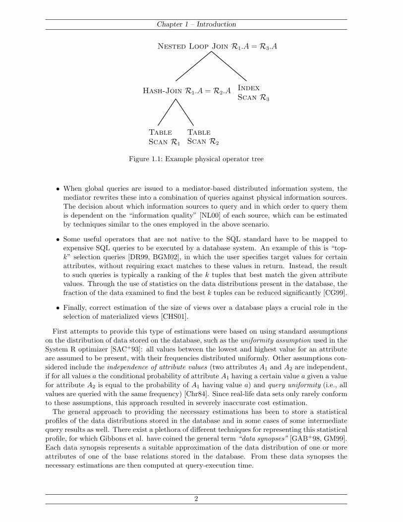
Chapter 1 – Introduction
TableTable
Hash-Join R1.A = R2.A
Nested Loop Join R1.A = R3.A
Scan R1 Scan R2
Scan R3
Index
Figure 1.1: Example physical operator tree
• When global queries are issued to a mediator-based distributed information system, themediator rewrites these into a combination of queries against physical information sources.The decision about which information sources to query and in which order to query themis dependent on the “information quality” [NL00] of each source, which can be estimatedby techniques similar to the ones employed in the above scenario.
• Some useful operators that are not native to the SQL standard have to be mapped toexpensive SQL queries to be executed by a database system. An example of this is “top-k” selection queries [DR99, BGM02], in which the user specifies target values for certainattributes, without requiring exact matches to these values in return. Instead, the resultto such queries is typically a ranking of the k tuples that best match the given attributevalues. Through the use of statistics on the data distributions present in the database, thefraction of the data examined to find the best k tuples can be reduced significantly [CG99].
• Finally, correct estimation of the size of views over a database plays a crucial role in theselection of materialized views [CHS01].
First attempts to provide this type of estimations were based on using standard assumptionson the distribution of data stored on the database, such as the uniformity assumption used in theSystem R optimizer [SAC+93]: all values between the lowest and highest value for an attributeare assumed to be present, with their frequencies distributed uniformly. Other assumptions con-sidered include the independence of attribute values (two attributes A1 and A2 are independent,if for all values a the conditional probability of attribute A1 having a certain value a given a valuefor attribute A2 is equal to the probability of A1 having value a) and query uniformity (i.e., allvalues are queried with the same frequency) [Chr84]. Since real-life data sets only rarely conformto these assumptions, this approach resulted in severely inaccurate cost estimation.
The general approach to providing the necessary estimations has been to store a statisticalprofiles of the data distributions stored in the database and in some cases of some intermediatequery results as well. There exist a plethora of different techniques for representing this statisticalprofile, for which Gibbons et al. have coined the general term “data synopses” [GAB+98, GM99].Each data synopsis represents a suitable approximation of the data distribution of one or moreattributes of one of the base relations stored in the database. From these data synopses thenecessary estimations are then computed at query-execution time.
2

Chapter 1 – Introduction
There are a number of important issues to consider regarding the construction and use of datasynopses.
• In all application scenarios outlined above, the data synopses need to support queries madefrom all three major logical database operators: selection, projection, and join (SPJ). Thisnot only entails being able to provide an estimation for the result (size) of each query type,but also having effective means to bound the estimation error for each query type. Manyof the existing approaches are geared towards minimizing the estimation error for range-selection queries only, and only very few techniques are capable of reducing the estimationerror for join queries effectively.
• Whenever the base data in the database is made up of relations over more than a singleattribute, the issue arises over which (combination of) attributes synopses should be con-structed. If no synopsis over a combination of two attributes exists, information over thecorrelation between the values stored in these attributes is lost. For example, in a relation Rwith the attributes Order-Date and Ship-Date, any query containing filter-conditions onboth attributes (e.g. “SELECT * FROM R WHERE |Ship-Date−Order-Date| ≤ 10”) wouldpotentially exhibit a significant estimation error. On the other hand, the accuracy of datasynopses is generally adversely affected by to the number of attributes it spans. Therefore,choosing the optimal combination of synopses for a given relational schema, the data distri-butions in the base relations, and the query workload is a complex optimization problem.Because finding a “good” combination of synopses requires significant knowledge about thedata distributions stored and the characteristics of the techniques used in connection withdata synopses, the decision which synopses to construct should not be left to the databaseadministrator, but instead has to be made by the database system automatically.
• In many cases it is not possible to optimize a query when it is first submitted to the databasesystem (this is referred to as the query’s compilation time), as some of the parameters whichdetermine the exact query statement may not be instantiated yet. These parameters arethen only specified immediately before the query is executed by the database (this is thequery’s execution time), so that any delay caused by the overhead of query optimizationis noticeable to the user. Because the estimation is invoked (possibly multiple times) forevery candidate plan (the number of which can be very large [Cha98]) at query executiontime, the estimation process itself may not result in significant overhead. Therefore, datasynopses are generally stored in main memory and thus have to be a small as possible, inorder not to take away space otherwise reserved for data caches or buffers for intermediatequery results. Consequently, the estimation accuracy relative to the amount of memoryconsumed becomes the critical measure when assessing the performance of data synopses.Furthermore, whenever multiple synopses are stored, the memory dedicated to data syn-opses overall has to be divided between them. This gives rise to a further optimizationproblem, which is closely connected to the question, which synopses to store overall.
The contribution of this thesis is to provide an overall framework addressing all of the issuesdiscussed above.
1.2 Problem Description
This thesis is concerned with examining two problem areas in the applications discussed above.The first one is how to construct synopses for accurate estimation using as little storage and
3

Chapter 1 – Introduction
computational overhead as possible. Based on these synopses the second problem area becomeshow to automatically compute the optimal combination of synopses for a given set of relations,a (characterization) of the system workload, and limits on the amount of memory available forall synopses overall; this I refer to as the physical design problem for data synopses.
In the following, I will introduce the general approach for addressing both problems and de-scribe by which criteria the proposed solutions will be evaluated. Throughout the thesis, I willdescribe the different requirements on and properties of data synopses using the query optimiza-tion as application scenario. However, whenever necessary I will describe the extensions necessaryfor other applications.
1.2.1 Synopsis Construction
All the outlined application scenarios require estimation of the result size for all major logi-cal database operators (select-project-join). A number of approaches [SLRD93, CR94, LKC99,MVW98], provide a function estimateΘ for each operator Θ, which takes the filter conditionsof a given query and returns an integer representing the number of tuples of the result. Forexample, a range-selection estimator selecting all tuples in a interval [a, b], with a, b chosen fromthe respective attribute’s domain D, is defined as
estimaterange : D ×D 7→ N.
Each of these estimators is then modelled as a function of two variables, resulting in a reductionof the estimation problem to a problem of the well-researched field of function estimation.
However, most real-life database queries consist of a combination of multiple operators, sothe above approach infeasible: because now all possible combinations of operators correspondto separate estimate functions, the number of functions becomes too large. Instead, for eachrelation stored in the database, an approximate representation of the underlying data distributionis stored. Now, when executing a query operator, this operator is executed on the approximatedata distribution. Any property of the approximate data distribution such as size (relevant forthe approximation of the cost of join queries), the number of different attribute values (relevantfor size estimation in queries with duplicate elimination or grouping), skew (relevant for providingsufficient memory for large join computation), etc. can be derived directly from the approximatedata.
While this approach makes it possible to estimate virtually every query operator, it does notnecessarily result in accurate estimation. I will discuss which requirements are necessary to ensureaccurate estimation of the three major logical operators and how these requirements are reflectedby different design choices for query estimation techniques.
Criteria for Success
In the query-optimization scenario, the benefit provided by a synopsis lies in the improvement inplan selection. However, this measure is heavily influenced by the particularities of both the queryworkload and the optimizer itself. Therefore, the estimation accuracy provided by a synopsis isused as a measure of its quality instead. Better estimation accuracy typically leads to betterplan selection as well, but there is not necessarily a direct correspondence: in some situations,even extremely poor estimation may have no adverse effect on plan selection, if the ranking ofthe candidate plans remains unchanged.
The accuracy of estimation itself is important when using result-size estimation to estimatethe overall running time of a resource-intensive query, in order to schedule it or decided whether
4

Chapter 1 – Introduction
to spawn it at all, as the absolute running time is the deciding factor for this decision. For sometypes of decision-support queries, knowing the size of the final query result before issuing it isalso useful in assessing whether a query returns compact enough information to be handled bya human user. If not, it may be necessary to add some aggregation or issue a different queryaltogether. In each case, the necessary information on query cost and result size need to beassessed as accurately as possible.
Because data synopses are stored in main memory, the accuracy of a synopsis has to be judgedrelative to the amount of memory its storage consumes. In addition to the memory overhead, thecomputational overhead required for (a) the construction and (b) the evaluation of a synopsisneed to be considered as well.
1.2.2 Physical Design Problem for Data Synopses
The optimal combination of synopses is dependent on three factors: (a) the characteristics of thedata stored in the database, (b) the current workload, and (c) the amount of memory available forsynopses overall. Initially, all possible combinations of synopses that can be used to answer thegiven mix of queries are determined. Among them, the combination is selected that minimizesthe estimation error for all attribute values selected by the given set of queries (with each error-term weighted by the number of times the corresponding attribute value is selected). Note thatthis does not only involve the selection of the optimal set of synopses, but also determining howthe available memory is divided among them.
Criteria for Success
Estimating all possible combinations of synopses and their sizes results in additional overhead,which commercial database systems avoid by using much simpler schemes for synopsis selection.In most cases, only synopses over single attributes are employed, with all synopses of equal size(which severely limits the queries that can be estimated accurately in itself). In order to justifythis additional overhead, the additional estimation accuracy gained through our more elaborateapproach needs to be significant.
In addition, an algorithmic solution to the physical design problem would be a step towardseliminating synopsis selection from the responsibility of a database administrator. Since choosinga good set of synopses requires in-depth knowledge of the data and the techniques used forquery estimation, and in addition this set needs to be periodically adapted to evolving workloadproperties, this task is not well-suited to human administration.
1.3 Contribution and Outline
The remainder of this thesis is divided into 5 chapters:
In Chapter 2, the design space for data synopses is discussed, with the different design alter-natives illustrated in terms of previous approaches. With regard to most design alternatives, itis possible to identify one design choice as clearly superior; these choices are then incorporatedinto the design of my own approach to data synopses. In addition, based on this system of designalternatives, I construct a taxonomy for the plethora of techniques proposed in related work.
Chapter 3 describes how to solve the limited problem of query estimation for queries on a singleattribute only. The salient property of the approach is that – unlike all other approaches to data
5
Chapter 1 – Introduction
synopses – separate and independent approximations are used for the distribution of the attributevalues and the distribution of their frequencies. Consequently, more memory can be assigned tothe more difficult or important approximation problem. In both cases, the approximation isreduced to a problem of linear fitting, with the attribute values and their frequencies beingapproximated through linear spline functions. The resulting technique has been named splinesynopses.
The chapter further elaborates the computation, storage, and use of spline synopses for queryestimation. Special attention is given to join queries, because unlike all other operators, accurateapproximation of the joining relations does not necessarily result in accurate join estimation.This leads to the introduction of special join synopses capturing the distribution of attributevalues that appear in the join result. Finally, the efficiency and accuracy of spline synopses isevaluated in comparison to the current state of the art through experiments on various syntheticand real-life datasets. In the experiments, spline synopses consistently outperform the best his-togram techniques, while being of identical computational complexity.
Chapter 4 then extends the previous approach to datasets and queries on multiple attributes.Here, the Sierpinski space-filling curve is used to map the multi-dimensional data to a linearlyordered domain, over which the approximation is then constructed. This approach leverages theadvantages of one-attribute spline synopses (efficiency, fast computation, independent represen-tation of attribute values and their frequencies) while avoiding the problems normally inherentto multi-dimensional synopses (distortion of the attribute-value domain, intractable overheadfor synopsis construction). Again, the efficiency of the resulting synopses is evaluated throughexperiments. Again, spline synopses outperform histograms, while offering accuracy competitivewith the best specialized techniques geared towards the limited class of range-selection queriesonly.
Chapter 5 finally discusses the physical design problem for data synopses, i.e., how to computethe optimal combination of synopses for given workload, data, and available memory. Initially,a formalization of the problem is developed through which the overall problem can be solvedthrough the enumeration of all potential synopsis combinations and a minimization over the ap-proximation errors computed during synopsis construction. This approach returns the best setof synopses as well as how much of the available memory is given to each of them. To reduce thenumber of synopsis combinations that need to be considered, the search space is pruned basedon two general observations on the behavior of data synopses. Since these observation not onlyhold for spline synopses, but for a large class of data synopsis techniques, a limited form of thesolution can be extended to these other techniques, as well. The practicability and potentialimpact of the proposed solution is evaluated on a subset of the queries and data of the TPC-Hdecision support benchmark.
Finally, chapter 6 offers a summary of the work and outlines future areas of research. Prelim-inary results of my work have been published in [KW99, KW00, KW02].
1.3.1 Limitations of This Work
The techniques described in this thesis are limited to numerical data (for both discrete andreal domains). Although string data can be mapped to N using enumeration schemes, someof the operators specific to strings (such as prefix- and substring-matching [JNS99]) can notbe estimated accurately when approximating this data using spline synopses (or any other of
6

Chapter 1 – Introduction
the approximation techniques discussed in the next section). This is due to the fact that theseoperators require the approximation technique to maintain the correlation between adjacentoccurrences of characters (or substrings). Because the approximation techniques used queryoptimization are geared towards representing other types of correlation, string data requires adifferent type of approximation, such as (approximate) suffix trees [NP00, JNS99, Ukk93]. Howto reconcile both classes of approximation techniques for estimation of queries requiring bothtypes of functionality is an open research problem at this time.
7

2 Related Work
One of the problems of taking things apart and seeing how they work– supposing you’re trying to find out how a cat works – you take thatcat apart to see how it works, what you’ve got in your hands is anon-working cat. The cat wasn’t a sort of clunky mechanism that wassusceptible to our available tools of analysis.
– Douglas Adams
This chapter gives an overview over work related to the topics of this thesis. When describingthe different approaches it is necessary to identify their distinguishing characteristics concerningdetails of how relational tables are approximated. Therefore, it is first necessary to introducesome notation in Section 2.1. In Section 2.2 the the necessary concepts regarding query processingare briefly reviewed. Section 2.3 provides a compact introduction to relevant aspects of queryoptimization. In Section 2.4 all previous approaches for result (size) estimation are introduced.In order to provide a classification of these as well as our own work, I initially discuss the designspace for query estimation techniques by introducing the most important design alternatives inthis domain. Previous approaches to the less studied problem of physical design of data synopsesare then discussed in Section 2.5.
2.1 Notation
Relational database systems store data in relations, which can intuitively be thought of as tableswith a certain number of rows and columns. Each row is referred to as a tuple, each column isreferred to as an attribute. An example relation is shown in Figure 2.1.
Employee ID Name Age Salary1076 Lennon 35 50.0001077 Harrison 49 75.0001078 Watters 18 15.000
Table 2.1: Example of a relation
In the following work, I consider a set of relations R = {R1, . . . , Rn}. Each relationRi ∈ R has atti attributes Att(Ri) = {Ri.A1, . . . , Ri.Aatti}. The values for each of these At-tributes Ri.Aj are defined over a domain DRi.Aj of possible values. The value set VRi.Aj ⊂DRi.Aj ,VRi.Aj = {v1, . . . , vn} is the set of values for Aj actually present in the underlying relationRi. The density of attribute Ri.Aj in a value range from a through b, a, b ∈ DRi.Aj , is the numberof unique values v ∈ VRi.Aj with a ≤ v < b. The frequency fk of value vk is the number of tuplesin R with value vk in attribute Ri.Aj . The cumulative frequency ck of value vk is defined as

Chapter 2 – Related Work
the sum of all frequencies fl for tuples vl < vk (i.e., ck =∑k−1
l=1 fl). The spread si of value vi isdefined as si = vi+1 − vi (with sn = 1). The area ai of value vi is defined as ai = fi · si.
Definition 2.1 (Data Distribution) :Based on the above, a (one-dimensional) data distribution over a single attribute Ri.Aj
is defined as the set of pairs TRi.Aj = {(v1, f1), (v2, f2), . . . , (vn, fn)}, with fk being thefrequency of value vk. When it is clear or immaterial which relation and attribute arereferred to, the subscript Ri.Aj is dropped when defining data distributions, domains, andvalue sets.
To give an example, consider a unary relation R1 over the domain DR1.A1 = N containing thefollowing tuples t1 = 10, t2 = 10, t3 = 20, t4 = 31, t5 = 40, t6 = 40, t7 = 40, t8 = 70, t9 = 90. ThenVR1.A1 = {10, 20, 31, 40, 70, 90} and TR1.A1 = {(10, 2), (20, 1), (31, 1), (40, 3), (70, 1), (90, 1)}.Definition 2.2 (Joint Data Distribution) :
A joint data distribution over d attributes Ri.Aj1 , . . . , Ri.Ajdis a set of pairs
TRi.Aj1,...,Ri.Ajd
= {(v1, f1), (v2, f2), . . . , (vn, fn)}, with vt ∈ VRi.Aj1× · · · × VRi.Ajd
and fk
being the number of tuples with value vk. In the following we use the general term datadistribution to refer to both single-attribute and joint data distributions.
The cumulative frequency ci of a value vi = (v1i , . . . v
di ) is defined as ci =
∑k∈{1,...,|TRi.Aj1
,...,Ri.Ajd|}
v1k≤v1
i∧...∧vd
k≤vd
i
fk.
It is sometimes necessary to strip tuples of some of their attributes. For this, I use the opera-tor |A with the set of attributes A describing the attributes, whose values remain after the opera-tion. For example, if t1 denotes the first tuple in table 2.1, then t1|{R.Age,R.Salary} = (35, 50.000).
Some approaches to data synopses provide their estimation in the form of an approximatedata distribution. In order to distinguish between the original data and its approximation,the approximation of the attribute value vi is denoted by vi and correspondingly the ap-proximation of frequency fi by fi. Thus, an approximate data distribution is written asTRi.Aj = {(v1, f1), (v2, f2), . . . , (vn, fn)}.
Definition 2.3 (Frequency Distribution, Cumulative Frequency Distribution) :Many approaches reduce the part of the estimation problem to a problem of functionestimation by treating a (joint) data distribution as a function f : VRi.Aj 7→ N with f(vi) =fi. This f is referred to as the frequency distribution function.
The cumulative frequency distribution function is defined analogously, but with f(vi) = ci.
While most of the mathematical notation in this thesis is standard, I use a notation introducedin [Ive62] that allows simplifying most case statements. The idea is to enclose a true-or-falsestatement in brackets, which is treated as a mathematical expression with result 1 if the statementis true, and result 0 if the statement is false. For example, [12 is prime] = 0 and [102 = 100] = 1.
As many variables used in this thesis have both subscripts and superscripts (e.g., x1k, . . . x
nk)
these can easily be confused with exponents. For this reason, all exponents (when applied tovariables) are separated from these by parentheses (i.e. (x)2 = x · x).
9
Chapter 2 – Related Work
2.2 Query Processing
Throughout this thesis, I will concentrate on the estimation of three major query operatorsSelection, Projection and Join. The reason for this focus is that most queries specified in the SQLdatabase language (which is the standard adopted by all commercial database systems [O’N94])can be specified as a combination of these 3 operators. To illustrate this, it is first necessary toexplain the basic SQL syntax. The basic form of an SQL query is a follows:
SELECT [DISTINCT] result−attributesFROM relations[WHERE selection-condition ][GROUP BY group-attributes [HAVING selection-condition]]
with relations specifying a subset of R; the set
A :=⋃
R′∈relations
{R′.A1, . . . , R′.A|Att(R′)|}
denotes all attributes present in these relations. Then result-attributes is a subset of A specifyingthe attributes present in the query answer. Each selection-condition specifies a filter on the tuplesselected. Only tuples, for which the filter condition holds are included in the query answer. Aselection-condition is of the form
selection-condition := [[NOT] A1 θ A2 [{AND | OR} selection-condition]|True|False]
with A1 ∈ A, A2 ∈ A ∪ DA1 and θ specifying a binary comparison operator from {<,≤,=,≥, >, 6=}. Depending on the underlying domains, some limited mathematical expressions are alsopossible for A1 or A2. In addition, it is possible to use results of different SQL queries (which arethen referred to as sub-queries) in place of A2 in a selection-condition. This extension gives SQLthe expressive power of first-order predicate logic. While our approach is capable of estimatingthis type of nested queries, I will focus on selection conditions limited to propositional logic.
It is further possible to specify aggregation operators in on single members of the result-attributes, that return an aggregate of the values in the respective column. The possible op-erators are (a) Count, (b) Sum, (c) Avg, (d) Max, and (e) Min, which specify (a) the numberof values, (b) the sum of the values, (c) the average of the values, (d) the highest value and (e) thelowest value in the column. These operators may also be used in a selection-condition followinga HAVING clause.
The result of a query specified through an SQL statement is another table, which containsall tuples present in the cross-product of the relations in relations, except for the tuples thatdo not satisfy the selection-condition and the attributes not present in result-attributes. Thus,SQL queries are operations on tables that also have results in the form of tables. The DISTINCTkeyword is optional. It indicates that the table computed as an answer to this query shouldnot contain duplicates (i.e., two copies of the same tuple). If DISTINCT is not specified, thenduplicates are not eliminated; so the result can be a multiset. Finally, the result of a query may bepartitioned into groups using the GROUP BY and HAVING clauses. Here the set group-attributes⊆ Aspecifies which combinations of attributes determine the grouping, i.e., all tuples that have thesame value for the attributes in group-attributes are assigned to the same equivalence class. Theselection-condition in the HAVING clause can specify additional conditions on the groups selectedin the final query result. Note that expressions appearing there must have a single value pergroup; therefore, aggregation operators are often used here.
10

Chapter 2 – Related Work
A query can now be answered using selection, projection and join operators, I now define theirsemantics with regard to data distributions. Data distributions are equivalent to the relationsor query results they represent in the sense that it is possible to reconstruct these from thedata distribution(s) over all attributes that either (a) are selected by the query (i.e., they arespecified in the result attributes clause) or (b) appear in the query’s filter conditions (i.e., theyare contained in at least one selection-condition). Thus, by defining the semantics of an operatorwhen applied to a data distribution, it is implicitly defined when applied to (part of) a relationas well. The operator semantics are defined as follows:
Selection: A selection over a selection-condition P is defined as an operation Select[P ] mappinga (joint) data distribution TA over a set of attributes A ⊆ A to a (joint) data distributionT ′A with
Select[P ](TA) = {(vi, fi) | (vi, fi) ∈ TA ∧ P (vi)}.A special sub-class of this query class are range-selection queries, which are characterizedby every attribute having filter condition of type
P := A1 ≤ constant1 ∧A1 ≥ constant2.
Note that with the exception of aggregation operators, all selection conditions in the WHEREclause express predicates on the attribute values present in the data distribution. Thismeans that any technique capable of estimating arbitrary selection conditions has to storean (approximate) representation of the attribute value distribution.
Projection A projection of a data distribution TA over a set of attributes A ⊆ A onto a set ofattributes A′ ⊂ A is defined as follows.
Project(TA) = {(v′, f ′) | v′ = vi|A′ ∧ vi ∈ VA ∧ f ′ =∑
(vi,fi)∈TAv′=vi|A′
fi}.
Intuitively this means that all tuples in TA, that are indistinguishable when considering onlythe attributes in A′ are combined into one tuple in the result returned by the projection.
Join A join is an operation over two data distributions TA = {(v1, f1), . . . , (vn, fn)}, TA′ ={(v′1, f ′1), . . . , (v′h, f ′h)} and a simple selection-condition P of the type P := [A1 θ A2 | True]with A1 ∈ A and A2 ∈ A′. The result is a data distribution TA∪A′ over the union of theattributes of TA and TA′ defined as
Join[P ](TA) = {(v, f) | v ∈ DA∪A′ ∧ v|A = vi ∈ VA ∧ v|A′ = v′j ∈ VA′ ∧ vi|A1 Θ v′j |A2 ∧ f = fi·f ′j}.In the special case of the selection-condition being True, the join result is identical tothe cross-product of the tables corresponding to TA and TA′ . Throughout this thesis Iconcentrate on joins with the selection condition of the form A1 = A2 (this type of join iscalled equi-join), as it is the most common and also the most difficult to approximate (thisis discussed in detail in Section 3.4.3). To denote the data distribution resulting from anequi-join between two relations Ri, Rj over the condition Ri.Ak = Rj .Al I use the notation
RiAk=Al
./ Rj .
For the sake of simplicity, assume that all selection conditions are connected via AND (this isnot really a limitation as all queries involving OR can be reformulated as the union of multiplequeries that only use AND). Now the evaluation of an SQL query as described above query canconceptually be described through the use of the above operators.
11
Chapter 2 – Related Work
1. First, for all sub-conditions A1 θ A2 in the selection-condition with A1 and A2 from differentrelations, compute the join over the involved relations. Then compute the cross-product(using the join operator) of the intermediate result(s) and all tables in relations whichwere not included in the first pass of joins. The result of these steps corresponds to thecross-product over all relations in relations, after all tuples not satisfying the sub-conditionsbetween relations have been removed.
2. From this intermediate result, select all the tuples satisfying the remainder of the selection-condition.
3. Through projection, remove all the attributes not appearing in result-attributes.4. If DISTINCT is specified, all frequencies in the resulting data distribution are set to 1.
While the above approach will result in the correct answer, it is in most cases not efficient, forsome tuples may be created only to be removed later. In order to make the execution of a querymore efficient, the single join, project, and select operations are reordered through the queryoptimizer in such a way that the query result stays the same. To assess the efficiency of queryexecution by different plans (i.e., operator orderings), information on the size, (and in some casesalso the data distribution) of relations and intermediate results is needed.
Definition 2.4 (Result Estimation, Size Estimation, Selectivity) :Estimation techniques used in query optimization can be distinguished by what type ofestimate they return. When given a query and data distribution the query is applied to,most techniques return an estimate for the size (expressed as the number of tuples) of theresult. This is referred to as query result size estimation. The fraction of tuples from theoriginal data still present in the query result is referred to as the selectivity of the query.
In contrast, other techniques provide an estimation of the result data itself (in the form ofa data distribution T ). All necessary aggregate information, such as the size, can than becomputed from T . This is referred to as query result estimation.
2.3 Query Optimization
Different approaches to query optimization can be classified by when the optimization for a givenquery is performed.
Static or compile-time optimizers (for example, IBM’s System-R query optimizer [SAC+93]) op-timize a query at the time it is being compiled, thereby avoiding additional overhead at run-time,and potentially assessing a larger number of query execution plans, because the optimization timeis less critical. This, however, is problematic as parameters important to the cost computation(such as available disk bandwidth, processing power and search structures, set cardinality or pred-icate selectivity) may change between compile-time and run-time, resulting in sub-optimal queryplans. More significantly, in many cases, not all parameters determining a query may be knownat compile-time (for example, when query parameters are specified remotely via host-variablesof a web session). In addition, when queries are specified through tools that generate SQL state-ments directly, compile and execution time may fall together. As a result, static optimizationcan only be applied to a limited number of application scenarios.
An alternative approach is dynamic query optimization [Ant93, CG94, AZ96] (used in OracleRdb), which chooses the execution plan at run-time, thereby benefitting from accurate knowledgeof run-time resources, host variables, and result sizes for sub-queries that have already beencomputed. However, in order to restrict the time necessary for optimization, a large part of the
12

Chapter 2 – Related Work
plan is still optimized statically [Ant93]. Thus, good estimation of intermediate result sizes isstill necessary. Another alternative is parametric query optimization [INSS97] which (at compile-time) generates the optimal plan for several potential values of the parameters on which thechoice of the optimal execution plan is contingent and (at run-time) selects among them.
A hybrid approach called dynamic query re-optimization [KD98] (implemented in the Paradisedatabase system [PYK+97]), collects statistics at key points in the execution of complex queries,which are then used to optimize the remainder of the query by either improving resource allocationor changing the execution plan.
A different approach to dealing with inaccurate result-size estimation at the level of the opti-mizer is presented in [SLMK01]. IBM’s DB2 optimizer [GLSW93] monitors query executions anduses the feedback to compute adjustments to cost estimates and statistics, which are then usedin future optimizations. These future optimization are again subject to monitoring, resulting in afeedback loop. As the adjustments themselves have very limited expressive power (mostly factorsthat are multiplied to the original estimates) they cannot replace query estimation techniques;so this approach does not invalidate the need for query estimation that is accurate in the firstplace.
2.4 Query Result Estimation
2.4.1 Design Space for Data Synopses
Recent research in the area of data synopses has led to a plethora of techniques providing thenecessary functionality. In order to categorize all available techniques for query estimation, I nowdescribe a number of different features characteristic for the different approaches:
Size Estimation vs. Result Estimation
As mentioned before, many techniques estimate only the size of the query result, providing theestimation for a query operator Θ ∈ {selection, projection, join} by approximating a functionwith dimensionality equal to the number of parameters of Θ representing the correspondingfrequency distribution function. For example, a range-selection over a single attribute R.A queryselecting all values in the interval [a, b) can be represented by the 2-dimensional cumulativefrequency function f . For example, to estimate a range selection over a single attribute R.A, thecumulative frequency function f , the approximation of which we refer to as f . Now, the resultsize of a range query selecting all values in the interval [vi, vj) is then estimated1 as Sel[i,j) :=f(vj) − f(vi). The estimations for other operators are then provided using a different functionfor each operator. Because estimations provided by these different functions cannot be combinedwithout additional information on the data distribution, additional functions would have tobe constructed and approximated to provide estimations for queries using multiple operators.Because the number of different operator-combinations occurring in real-life database applications
1For d-dimensional distributions the result size of a selection (v1i ≤ R.A1 ≤ v1
j ) ∧ . . . ∧ (vdi ≤ R.Ad ≤ vd
j ) is
estimated using the d-dimensional function f approximating the cumulative frequency as follows:
Sel[i,j) :=X
xk∈{vki
,vkj}
1≤k≤d
dY
l=1
−1[xl=vli]
!· f(x1, . . . , xd)
!.
13

Chapter 2 – Related Work
is large, this approach is not practical for query optimization. Furthermore, the approach failswhen the filter-predicates are more complex than the range-selection example above.
Example 2.1: Consider the query
SELECT DISTINCT R.Order-date FROM R WHERE |Ship-Date−Order-Date| ≤ 10.
While approaches that approximate the (cumulative) frequency distribution function arecapable of estimating the number of tuples for any possible value of Ship-Date or Order-Date, they have no representation of the value domain itself, so the (number of) actualvalues in the result cannot be estimated.
The problems discussed in the above example stem from the fact that these types of techniques– when given a range of attribute values – offer accurate estimation of the number of tuples(or values, when Θ =projection) in that range; however they do not offer any information onwhich attribute values vi are contained in V (the only way this information can be gatheredis by checking whether a given value has a frequency different from 0, which typically leadsto significant overestimation of the number of unique values). Summing up, one may say thattechniques that approximate the (cumulative) frequency function only offer good approximationof the value frequencies fi, but not of the values vi themselves. To make this distinction explicit,we introduce the following notation.
Definition 2.5 (Value Frequency Approximation, Value Density Approximation) :When approximating a given data distribution T , the technique used for representing theattribute value frequencies f1, . . . , f|T | is referred to as the value frequency approximation.
The technique used for representing the attribute values v1, . . . , v|T | occurring in T them-selves is referred to as the value density approximation.
In order to deal with the above problems, a number of approaches use techniques capable ofestimating the query result itself and not only its size, meaning they store the approximatedata distribution T of a relation stored in the database and apply operators directly to thisdistribution. The result of each operation is another approximate data distribution, to whichfurther operators may be applied. Because the approximation contains information on both theattribute values and their frequencies, all potential filter conditions can be applied.
The potential drawback of this approach is the fact, that providing estimation of the queryresult itself potentially requires more computational overhead, than the query-result size becausepotentially the entire data-distribution has to be materialized (consequently, the computationaloverhead for computing result size estimation is typically lower). Still, only techniques capableof estimating the query result as well are capable of dealing with the wide range of selectionpredicates occurring in real-life applications; thus, only query result estimation techniques aresuitable candidates for the support of query-optimization.
Support for different Operators
An estimation technique needs to be able to support estimations for all major operators: selec-tion, projection, join. However, offering the functionality of estimating a query operator resultis meaningless if the technique is not capable of bounding the corresponding estimation erroreffectively.
For example, a large number of techniques are geared towards minimizing the variance in fre-quency approximation error only, i.e. synopsis construction selects the synopsis with the smallest
14

Chapter 2 – Related Work
error-function f err :=∑|T |
l=0(fi− fi)2. This minimizes the estimation error for a class of equalityqueries(equality queries of type R.A = x under the assumption that only values x ∈ VR.A arequeried) and is effective in minimizing the error for range-selection queries [IP95]. However, forjoin queries this approach fails, as accurate placement of the approximate attribute values is notin any way reflected in the error-function f err. Therefore, the number (and approximate value)of attribute values finding a join-partner when estimating an equi-join query may be significantlyoff, leading to large estimation errors when computing a join over a data distribution (see Sec-tions 2.2). Adding more memory to the corresponding synopses does not necessarily alleviatethis problem, but may make it worse. In essence, this rules out approaches minimizing f erronly, when join queries need to be estimated.
Because most research in the area of data synopses has been geared towards improving range-selectivity estimation, a large number of approaches result in problems of the described nature forjoin and projection queries, the specifics of which will be discussed in Sections 4.1 (for projectionqueries) and 3.4.3 (for joins). In summary, data synopses need not only support operators, buthave to be able to reduce the corresponding errors effectively.
High-dimensional Data
When estimating queries specifying filter conditions on more than one attribute of a relation, itbecomes necessary to take into account the correlation between multiple attributes of the data.To illustrate this, consider the following example: Given a table Employees, containing theattributes Height (in centimeters) and Weight (in kilograms). Now consider the query
SELECT * FROM Employees WHERE Height < 160 AND Weight ≥ 100.
Assuming one has exact knowledge over both the data distribution THeight and the data distribu-tion TWeight, and the number of tuples satisfying the condition on Height is 20% of the relationand the number of tuples satisfying the condition on Weight is 25% of the relation. Still, withoutany additional information on the correlation present between the attributes, the only knowledgegained about the selectivity of the entire query is that its result contains between 0% and 20% ofthe relation. Many early approaches use the attribute value independence assumption [SAC+93]at this point, estimating the selectivity of the composite filter as 25/100 · 20/100 = 5/100, whichoften leads to significant estimation errors (in the example, the selectivity is likely to be closerto 0%). Consequently, even data synopses over single attributes that perfectly estimate theunderlying distributions do not permit accurate estimation for this type of correlation.
In order to provide accurate estimations for this type of queries, the data synopsis has to takeinto account the joint data distribution of the queried attributes. This entails preserving theamount of correlation present in the data.
Definition 2.6 (Correlation) :Correlation is defined for data points that have two values of different quantity; it measuresinhowfar the value of one quantity can be used to predict the value of another. In the aboveexample, Height is strongly correlated to Weight, as the taller a person is, the highertypically his weight. If two quantities are independent (for example: salary and shoe size),they are said to have zero or no correlation.
As this thesis is concerned with ordinal and particularly cardinal numeric attributes, it ispossible to use numerical measures of the present correlation. Depending on the context,the linear correlation coefficient [PTVF96] or the Spearman rank-order correlation coeffi-cient [PTVF96] are used. The latter is more robust with regard to quantities of radically
15
Chapter 2 – Related Work
different domains, as it does not measure the absolute values of the quantities, but theirrank within the respective domains.
For query (size) estimation two types of correlation are of importance: (a) the correlationbetween the multi-dimensional attribute values and their frequencies (this correlation is alsoknown as the skew of the value distribution) and (b) the correlation between the values differentattributes themselves. While most techniques focus on the first problem, both of them are equallyimportant for query estimation, which will be discussed in more detail in Section 3.4.3.
Handling of Data Updates
Because the data distributions approximated through data synopses are subject to change when-ever the corresponding relations or data sets are updated, these changes have to be propagatedto the data synopses as well. For this reason, some approaches offer the option of incrementalupdates which either use feedback obtained from observing the actual query results or monitorupdates, deletions and insertions on the data itself and propagate these to the relevant synopses.
Unlike the previously discussed features, where it was possible to identify a ’correct’ designalternative, there is a trade-off between flexibility towards updates and estimation accuracy.Because efficient compression (i.e., data reduction) schemes are generally very sensitive to changesin the data to be compressed, a single insertion, deletion or update may require a completereconstruction of the corresponding synopses. This means that substantial overhead for synopsisconstruction is incurred whenever data is changed, which is prohibitive in real-life applications.On the other hand, data synopses that immediately integrate updates immediately with onlynegligible overhead generally offer significantly less data compression and thus typically worseestimation accuracy within the given memory space. Furthermore, when too many updates areperformed, synopses based on this type of techniques may even require complete reconstruction.
As the memory required to store data synopses is normally a critical resource, it is oftenpreferable to construct synopses that do not immediately integrate changes to the data andreconstruct these synopses during low system load whenever the data has changed significantly.While these synopses degrade over time when not updated, their accuracy is typically superiorto begin with, thereby freeing up more space for cache and buffer memory.
2.4.2 Approximation Techniques
The final characteristic feature of approaches providing data synopses is the technique they usefor data reduction. In the following, I introduce the most important classes of techniques.
Histograms
Histogram techniques [PSC84, Poo97, PIHS96, JKM+98, MD88, PI97, BCG01] approximate adata distribution T by partitioning it into disjoint intervals called buckets. In one-dimensionalhistograms (for one attribute) each bucket stores the sum of the frequencies of the attributevalues contained in the corresponding interval, the number of distinct values in the interval andthe highest attribute value. In multi-attribute histograms each bucket stores the sum of thefrequencies of the attribute values contained in the interval, and for each attribute the lowest andhighest value contained as well as the number of distinct values2. There exist a large number of
2A more space-efficient way of storing multi-dimensional histograms is introduced in [DGR01].
16
Chapter 2 – Related Work
different histogram variants; the different classes can be classified by three3 parameters:
Sort Parameter Specifies which domain is partitioned into histogram buckets (the choices beingattribute values, frequency, and area).
Partition Constraint A mathematical constraint on the source parameter that uniquely identifiesthe rule by which the domain of the sort parameter is partitioned.
Source Parameter A parameter derived from the distribution T (the choices being attributevalue spread, frequency, cumulative frequency, and area) used in the partition constraintto identify the unique bucketization.
A complete taxonomy of histogram variants can be found in [Poo97]. A histogram characterizedin this way is generally described in the following notation:
Partition-Constraint (Sort-Parameter, Source-Parameter)
For example, the well-know Equi-depth histograms, which choose their buckets in such a waythat the sum of the frequencies in each bucket is (approximately) equal among all buckets, arewritten as Equi-Sum (V,F).
The most important class of single-attribute histograms use the partitioning constraint V-Optimal , meaning the buckets are chosen in such a way that the variance between the actualvalue and its approximation of the source parameter is minimized (i.e., if the source parameteris frequency, the error function f err :=
∑|T |l=0(fi − fi)2 is minimized).
It can be shown that V-Optimal(F,F) histograms [IC93, Ioa93, IP95] are optimal for estimatingthe result size of tree join, equality join and selection queries. However, as this type of histogramuses frequency as sort-parameter, information on the exact position of each attribute value has tobe stored explicitly to use this histogram type for estimation, resulting in O(n) storage overheadand rendering this type of histogram pointless for real-life applications, as the correspondingdata distribution T itself could be stored using less space. The histogram types generally usedin practice are V-Optimal(V,F), V-Optimal(V,A) and Max-Diff(V,A) histograms, as they offerthe best performance for a wide range of data distributions and queries [PIHS96]. Once the datadistribution T is known, construction of an histogram with m buckets requires O(m · |T |2) over-head for V-Optimal histograms [JKM+98] and O(log2 m · |T |) for Max-Diff histograms [PIHS96].Producing a query result estimation requires O(|T |) cost when histograms are used; if only theresult-size is of interest, the cost is O(m).
When constructing histograms over multi-attribute distributions, the problem of partitioningthe attribute value domain in such a way that the variance of a source parameter over all bucketsin minimized becomes NP-hard [MPS99]. Thus, any variant of V-Optimal histograms resultsin unacceptable computational overhead in practice. In [MD88] a multidimensional variant ofthe well-know Equi-depth histogram is introduced, which partitions the attribute value domainone dimension at a time into buckets enclosing (approximately) the same number of tuples.In [PI97] several alternatives were introduced, with the most accurate one being multidimensionalMax-Diff(V,A) histograms, which do not base their partitioning on the full multi-dimensionaldistribution, but choose the partitioning based on one-dimensional projections of the frequencydistribution.
3In [Poo97] a 4th parameter Partition Class is used, but as all histograms proposed in the literature are of theclass serial. This means that that buckets group elements from T that are contiguous in order and that thereis no restraint on the number of elements that may be assigned to a bucket.
17

Chapter 2 – Related Work
All the discussed multidimensional histograms are static in the sense that they cannot adaptthemselves to changes in the data distribution without reconstructing the histogram completely.To overcome this, [AC99, BCG01] introduce a new approach to histogram construction in thatthey observe the query workload and the query results and leverage this information for histogramconstruction. The resulting histograms are constructed on the fly and continuously updatedthrough new query feedback. This process not only reflects the data, but also locality in theaccess pattern of the workload, and the histograms of [BCG01] are more expressive in that theyallow overlap between buckets. Therefore, the resulting histograms often offer better accuracythan static multidimensional histograms.
While histograms are typically less accurate than the techniques discussed below, they are easyto construct, maintain and use. All types of histogram can be used to estimate a query result infrom of a data distribution [IP99] and may thus be used for estimation of virtually any query.For these reasons, histograms are used in virtually any commercial database system [Poo97].However, no histogram type is capable of providing both accurate estimation of attribute valuefrequency and attribute value density (see Section 3.2), which is problematic for estimating queriesrequiring accuracy in both domains (see Section 3.4.3).
Hybrid Techniques for Real-Valued Domains
[GKTD00] introduces a variant of multidimensional histograms aimed at continuous value do-mains (typically the set of real numbers R) called GENHIST (GENeralized HIStograms). Thepartitioning algorithm constructs progressively coarser grids over the data set, with each cellcontaining information on the density of values in the corresponding interval. The algorithmthen removes points from (combinations of) dense cells, storing an approximation of the removedtuples in a bucket. Not all tuples in the area are removed, but only sufficiently many so thatthe density decreases to the level of the neighboring cells. Thus creation of a new bucket has asmoothing effect on the remaining data, making it easier to approximate.
The resulting histograms show good estimation accuracy for range selectivity queries, but offerno support for other query types (because of the real domain, the authors assume that it isunlikely that a given attribute value will appear more than once – obviously, this assumption isviolated in most non-real domains). For this reason they are not grouped with other histogramapproaches in this classification.
In [BKS99], a different approach for real-valued value domains is introduced. Here, the so-called probability density function (PDF) F (x) =
∫ x−∞ f(t)dt over the frequency distribution
function f is modelled using kernel [Sco92] functions as density estimators. The partitioningalgorithm introduces bucket boundaries at points where the PDF is not sufficiently smooth tobe approximated using a kernel. Inside the buckets themselves, kernel estimators are used. Thisapproach is generalized to higher dimensions in [GKTD00]. Again, the resulting technique is notsuitable for queries other than range-selectivity estimation.
Parametric Techniques
Parametric techniques (also known as curve-fitting or regression models) [Chr83, Lyn88, SLRD93,CR94] approximate the data distributions using a mathematical distribution function with alimited number of free parameters (e.g., coefficients of polynoms). Values for these parametersare then chosen to fit the actual distribution. If the model is a good fit for the distribution, thisprovides an accurate and compact approximation; however, since the shape of the distribution isgenerally not known beforehand, this is often not the case.
18

Chapter 2 – Related Work
To gain some degree of flexibility, the approaches of [SLRD93, CR94] use a general polynomialfunction and apply least-squares fitting to choose its coefficients. To avoid both overfitting andthe corresponding fitting problem from becoming ill-conditioned [PTVF96], the degree of thepolynomials still has to remain small (both techniques use polynomials of degree less than 10).In addition, the approach of [CR94] leverages feedback from the actual result sizes to re-fit thecoefficients. Thus it is able to adapt to changes in the value distribution as well as to locality inthe ranges of the distribution being queried by improving the estimation of attribute values thatare queried more frequently.
Generally, parametric techniques only estimate result sizes, and are not capable of providingfull result estimation.
Discrete Transforms
A different approach to achieve the data reduction necessary for synopsis construction is to treatthe frequency distribution function f as a signal on which a discrete transformation is performed(such as the fast fourier transform(FFT) [PTVF96], the discrete cosine transform(DCT) [Lim90]or one of many possible wavelet transformation [SRS96]) returning |T | coefficients representingthe original signal. The constructed data synopses then only retains the most significant mcoefficients, from which an approximate frequency distribution function f is reconstructed atestimation time.
This approach is used in [MVW98], where the wavelet-transform (using Haar wavelets) isused on the cumulative frequency distribution function. To select the the m most significantwavelet coefficients, four different thresholding schemes are introduced, the first one selecting thecoefficients by the size of their absolute normalized value4 (thereby minimizing the error-functionf err :=
∑|T |l=0(f(vi)− f(vi))2 [SRS96]), and the other three greedy variants choosing coefficients
by their overall effect on the chosen error metric. The key feature here is that for all thresholdingschemes only the approximation of the value frequencies is examined. There is no approximationof the attribute-value distribution, resulting in a technique unsuitable for projection and joinqueries. While this effectively rules out this approach in the context of query optimization, it canstill effectively be used for approximate answering of OLAP range queries on multidimensionaldata cubes [VWI98, VW99]. In [MVW00], a framework for handling incremental updates isadded. The overhead for constructing the wavelet decomposition over a data distribution T isO(|T |), selecting m final coefficients through thresholding requires at most O(|T |·log2 |T |·log2 m)operations and the estimation of the size range query has overhead O(min{m, log |T |}).
To overcome the limitations of the previous approach, [CGRS00] approximates an frequencydistribution function f extended by adding the tuple (v′, 0) for all v′ ∈ D, v′ 6∈ V to the datadistribution. To exploit multi-dimensional locality, a different decomposition scheme is used; stillthe retained coefficients are selected by their absolute normalized values. While this approachmakes it possible to process aggregation, projection, and join operators, the approximation ofthe attribute value distribution is only a by-product of the fitting of the frequency distribution,meaning that the estimation error for this type of queries is not minimized (this phenomenonis discussed in more detail in Section 3.4.3). The significant contribution of this work is thatall operators are defined on the wavelet coefficients and also have wavelet coefficients as results,thereby eliminating the need to materialize intermediate results, and thus speed up the estimationof complex queries significantly.
4This means that a coefficient at resolution i is divided by√
2i. This way, coefficients that play a role in thereconstruction of a large number of frequencies have a correspondingly higher value.
19

Chapter 2 – Related Work
The basic approach of [LKC99] is similar to [MVW98] but a discrete cosine transformationis used here instead, as this transformation results in better energy compaction than the Haartransform [Lim90, RY90]. The final coefficients are then selected via geometrical zonal samplingmeaning that the coefficients are chosen by their geometric position, and not by their value.Because the DCT is linear transform5, incremental updates are realized by computing the coeffi-cients of the inserted/deleted data and adding/subtracting them to/from the stored coefficients.In contrast to [MVW00] any changes to the data do not result in a different set of coefficientsbeing retained, but is only reflected in the value of the coefficients selected earlier. Because noinformation on the attribute value distribution is stored, this approach is limited to selectivityestimation for range-selection queries.
Probabilistic Models
The techniques introduced in [DGR01, GTK01] approximate the frequency distribution functionby treating it as a probability distribution, which in turn is modelled through probabilistic rela-tional models [DGR01] or statistical interaction models [GTK01]. As only the value frequencydistribution is modelled, this results in the limitations discussed above; to make join approxima-tion possible [DGR01] extend their model by introducing binary indicator variables for attributevalues involved in equality joins which indicate whether or not the tuple is present in the joinresult.
2.4.3 A Classification of All Approaches
Summing up the different design alternatives discussed in Section 2.4.1, a data synopsis used forquery estimation should have the following properties: It needs to be able to provide estimationof the query result (and not only its size) , be able to express the correlations found in multi-dimensional data distributions, support selection, projection, and join queries, and must be ableto effectively minimize the estimation error for each query type. While the ability to update thesynopsis incrementally can save the cost incurred by synopsis recomputations, it generally resultsin less efficient data reduction6.
Table 2.2 characterizes all approaches discussed above with regard to these criteria. Eachcolumn signifies the ability of a given approach to provide the functionality stated at the top of thecolumn. Whenever this is the case, I reference the paper(s) in which this is described. Wheneverthe same paper appears in multiple columns, the approach introduced in it supports the features ofmultiple columns. On the other hand, the features of different papers are typically not compatible.For example, although both [SLRD93, CR94] are parametric techniques, only [SLRD93] supportsmulti-dimensional data and only [CR94] supports incremental updates. The only exception to thisrule are histogram techniques: all of them support all 3 major query operators (the correspondingtechniques being discussed in [PIHS96]) and all of them can be used for result estimation (asdiscussed in [IP99]).
The most important fact expressed through this classification is that even though query esti-mation has been extensively studied, no single technique is capable of bounding the estimationerror for selection, projection and join queries effectively (this will be discussed in more detail
5The DCT is linear in the following sense: Let Fc be the DCT, γ, δ scalars and x, y general k-dimensional vectors.Then it holds that Fc(γ · x + δ · y) = γ · Fc(x) + δ · Fc(y).
6The fact that the histograms of [BCG01] outperform multi-dimensional Max-Diff histograms is not a con-tradiction to this, but merely a reflection of the suboptimal partitionings generated through the MHIST-npartitioning algorithm. With regard to estimation accuracy, all other discussed techniques also outperformMax-Diff histograms by a wide margin.
20

Chapter 2 – Related Work
SPJ-queries SPJ-queries Multidimensional Query Result Incrementalsupported optimized distributions Estimation Updates
[PI97, AC99] [GMP97, AC99]Histograms all ([Poo97])[BCG01]
all ([IP99])[DIR00, BCG01]
HybridTechniques
[GKTD00]
Parametric [SLRD93, CR94] [SLRD93] [CR94]Discrete [VW99, CGRS00]Transforms
[CGRS00][LKC99, VWI98]
[CGRS00] [LKC99, MVW00]
ProbabilisticModels
[DGR01, GTK01]
SplineSynopses
√ √ √ √
Table 2.2: Functionality of the different approaches
in Sections 3.2 and 3.4.3). In addition, only histograms and [CGRS00] are capable of providingquery result estimation. Because both criteria are essential to accurate query estimation in thecontext of query optimization, query cost estimation is still considered an open issue in thiscontext [CG94, Cha98].
As for the problem of capturing the correlation present in multidimensional distributions, alarge number of approaches exist that are capable of maintaining multidimensional correlations.While histogram-based approaches suffer from a variant of the ”curse of dimensionality” causingunacceptable computational overhead for some histogram types [MPS99] and rapid decline inestimation accuracy with rising number of dimensions (this is discussed in detail in Section 4.1),most other techniques offer accurate estimation of multi-dimensional range-queries. However,the only non-histogram techniques capable of estimating joins and projections are [SLRD93,CGRS00].
Spline Synopses [KW99, KW00] offer both query result and size estimation for selection, pro-jection and join queries and consequently support estimation of all major query types. They canprovide estimation for queries over multiple correlated attributes. In addition, they are capableof minimizing the estimation error for range-selections (see Section 3.5.2), projections (see Sec-tion 3.5.2) and join-queries (see Section 3.4.4) efficiently. While spline synopses are not capableto incorporate changes to the data distribution without recomputing the entire synopsis, thisis a consequence of the efficiency of the techniques used forn data reduction. Spline synopsescompute the optimal representation (i.e., the representation with the smallest error) for anydataset they approximate. As this is a global optimum over the entire data, small changes in thedata may result in a completely different approximation, thereby causing the need for completerecomputation.
2.4.4 Sampling
Sampling-based techniques [HS92, HNSS95, Haa96, CMN98, GGMS96, LS95] provide result-sizeestimation by collecting a small random sample from the data and then scaling the result.
This approach works particularly well for certain types of aggregation: count, sum and average.Here the sample constitutes an unbiased estimator, with the expected value for performing theaggregation over the sample being equal to the result of the query itself. In addition, it is possibleto leverage the central limit theorem [Nel95] to obtain confidence intervals for the estimatedanswer.
21
Chapter 2 – Related Work
On the other hand, queries, where infrequent attribute values may significantly influence thequery result (e.g., join estimation, as discussed in [CMN99]), or estimation of the number of dis-tinct values for an attribute (as discussed in [CCMN00]) require a very large sample to guaranteea low estimation error. This is problematic, as the process of sampling the disk-resident data isslow. This is made worse by that fact that even to obtain a small sample, often a large number ofdatabase pages need to be read, as the tuples stored on a given page are often highly correlatedand thus do not constitute a random sample. As an alternative, some systems create a randomsample of the data called a reservoir sample [Vit85] and update it whenever updates, insertionsor deletions occur [GMP97, GM98]. This reservoir can then be accessed much more efficiently.While the reservoir sample could be stored in main memory and serve as a type of data synopsisthere, the size of such a sample is normally prohibitively large.
In summary, the applications of sampling and data synopses do not overlap significantly, asdata synopses are mainly concerned with the approximate representation of data distributions,and sampling with the approximate acquisition of them. Thus, I do not compare our approachto sampling techniques in this thesis. There is, however, a chicken-and-egg relationship betweensampling and data synopses. In many cases, when scanning an entire data set results in too muchoverhead, sampling is employed to obtain an approximate data distribution from which a datasynopsis for the given relation is then constructed [CMN98]. In addition, a reservoir sample (ondisk) can be used to incrementally reconstruct a data synopsis in main memory at much reducedcost [GMP97]. But data synopses can also aid sampling: when using sampling to estimate theresult of a join query (without computing the join itself), partial statistics on the high frequencyvalues are vital to the efficiency of the sampling algorithm [CMN99].
2.5 Physical Design of Data Synopses
The problem of selecting the optimal combination of synopses for a given combination of data andworkload has not received much attention until recently. This is problematic for in virtually allapplication scenarios for data synopses more than one synopsis is needed. While the techniquesdescribed above have resulted in increasingly accurate estimation, to a large degree the efficiencythus gained is lost through the use of overly simple schemas for selecting synopses and allocatingtheir memory.
The reconciliation of different synopses as well as dedicated synopses for join queries (a uni-form random sample over a foreign key join) was initially considered in [AGPR99]. These ideasare generalized in this thesis, as [AGPR99] is limited to samples as base synopses and a datawarehouse environment with a central fact table connected (via foreign keys) to the respectivedimension tables. An extension of this approach to incorporate workload information (in theform of access locality) can be found in [GLR00], but it is also limited to the above applicationscenario.
The reconciliation problem for spline synopses was first discussed in our own work [KW00],where a dynamic programming approach is proposed to minimize the error for a given set ofsynopses. However, this work offers no solution regarding which set of synopses to construct anddoes not take into account the characteristics of the workload. A similar approach for histogramswas proposed in [JJOT01], extending [KW00] by offering heuristics that reduce the overhead ofthe dynamic programming problem.
[CN00] considers a limited version of the problem: a set of synopses for query optimizationare selected, based on whether or not they make a difference in plan selection. However, theapproach is limited in a number of ways. Most importantly, synopsis selection is a series of yes-
22

Chapter 2 – Related Work
or-no decisions, with no consideration of the effect that variations of the size of a synopsis mayhave. This also has the consequence that the overall memory allotted to the selected synopses isutilized in a sub-optimal way. Furthermore, there is no consideration of special, dedicated (join-)synopses which do not constitute a (sub-)set of the attributes of a single relation.
The physical design problem for data synopses resembles the index selection problem for phys-ical database design, which has been intensively studied [FST88, CWBC95, RS91, CN99]. How-ever, there are a couple of fundamental differences between these two problems that make thesynopses problem much more difficult: (1) a synopsis not only chooses an attribute combinationon which it maintains statistics, but its quality is highly dependent on the memory allocated toit (e.g., for a certain number of buckets in a histogram), and (2) a synopsis on a proper subsetof attributes over which another synopsis is already maintained can be advantageous becauseof different approximation accuracies for different query types, whereas with B-tree indexes anindex on a subset of an already indexed attribute combination would (to a first approximation)be superfluous.
23

3 Approximation of a Single Attribute
Size matters not. Look at me. Judge me by mysize, do you?
– Yoda
In this chapter I address, the problem of building an approximation for a data distribution T ={(v1, f1), . . . , (vn, fn)} over a single attribute. The approach is similar to histogram techniquesin that the underlying value domain V is partitioned into buckets, which store a summary of thedata points contained in them. The way this is done in histograms has significant drawbacks: thepartitioning of V via buckets determines the quality of approximation for both attribute valuefrequency and value density. Thus, choosing a partitioning that results in a good approximation ofboth domains is often impossible, as these optimization goals are in conflict. Histograms thereforeare generally aimed at minimizing the estimation error for either the attribute value frequencies(all histograms with source-parameter Frequency) or attribute value density (source-parameterValues)1.
)UHTXHQF\�$SSUR[LPDWLRQ
Att
ribu
te v
alue
fre
quen
cy
Attribute value density
'HQVLW\�$SSUR[LPDWLRQ
��IUHTXHQF\�DSSUR[LPDWLRQ�EXFNHWV
��GHQVLW\�DSSUR[LPDWLRQ�EXFNHWV
Figure 3.1: Example of a spline synopsis
Consequently, spline synopses construct two different, independent approximations (and thus1Histograms with source parameter Area use an error function that aims to reconcile the approximation of both
domains, but merely place bucket boundaries at the points with the largest gaps in Area, thereby often failingto construct a good partitioning for either domain.

Chapter 3 – Approximation of a Single Attribute
partitionings) for capturing the frequency and the density distribution of an attribute (see Fig-ure 3.1). Not only does this eliminate the above problems, but as the number of buckets for eachdistribution is not fixed a priori, it also allows us to assign more memory to the more difficult(or more important) of the two approximation problems.
The construction of the approximation of attribute-value frequencies is described in Section 3.1and the approximation of attribute-value density in Section 3.2. Section 3.3 then describes howto combine the two different approximations and how to choose their sizes for a limited amountof available memory. In Section 3.4, I then discuss how to use the resulting spline synopsis forestimation. It turns out that accurate estimation of join queries requires additional information.This leads to an additional type of dedicated join synopsis, which is discussed in Sections 3.4.3 –3.4.6. The chapter concludes with an experimental evaluation of join synopses in Section 3.5.
In the following, it is assumed that there is a limit on the number of buckets, M , of the synopsisrepresenting T . The number of buckets for the two approximations is assumed to be set at m(for frequency approximation) and m′ (for density approximation) with M = m + m′. It will beshown that by generating the optimal partitioning for a given number of buckets, the optimalpartitioning for all smaller numbers of buckets is also generated at negligible additional cost.This property is exploited in Section 3.3.2, where I discuss how to choose the values of m and m′
in adaption to the difficulty of the corresponding approximation problems.
3.1 Approximation of the Attribute-Value Frequencies
To approximate a given value-frequency distribution T , the (observed) value set V is partitionedinto m disjoint buckets, bi = [vlowi
, vhighi) in the following manner, where lowi and highi denote
the subscripts of the values from V (i.e., not the actual values) that form the left and right boundsof the (left-side closed and right-side open) value interval covered by the bucket:
∀i ∈ {1, 2, . . . ,m− 1} : highi = lowi+1(low1 = 1, highm = n + 1). (3.1)
For the sake of a simple, uniform notation, T is extended by an artificial tuple (vn+1, 0) withvn < vn+1.
Unlike histograms, spline synopses approximate the frequency in an interval by a linear func-tion, resulting in a linear spline function [dB78, Die93] over the m buckets. Because my interestis in the compact representation of distributions and not in the features more advanced formsof splines offer (smoothness, differentiability), I have chosen simple linear spline functions forthis task. In contrast to previous approaches to spline-based histograms [PIHS96] these are notrequired to form a continuous approximation of T C+
, thereby simplifying the problem of find-ing the optimal partitioning (see Subsection 3.1.3) and increasing the resulting approximationaccuracy as well.
Using a linear function fi(x) = αi · x + βi to approximate the frequencies for the val-ues x in a bucket leads to an improvement in accuracy, depending on the linear correla-tion [PTVF96] of the data within a bucket. First, I define v[low,high) := 1
high−low
∑high−1l=low vl
as the average attribute value within [vlow, vhigh); analogously, I define the average frequencyf[low,high) := 1
high−low
∑high−1l=low fl. The linear correlation for interval bi is then defined as
r[lowi,highi) :=
highi−1Pl=lowi
(vl−v[lowi,highi))(fl−f[lowi,highi)
)
vuuthighi−1Pl=lowi
(vl−v[lowi,highi))2
vuuthighi−1Pl=lowi
(fl−f[lowi,highi))2
(3.2)
25

Chapter 3 – Approximation of a Single Attribute
For each interval bi, r[lowi,highi) ∈ [−1, 1]. In traditional histograms, the frequency in a bucket bi
is approximated by f[lowi,highi). Using the sum of the squares of the error at each frequency asan error metric, this results in the error for bucket bi if a histogram were used:
histogram err[lowi,highi) =highi−1∑
l=lowi
(fl − f[lowi,highi))2.
In a spline-based synopsis, using the same error metric the estimation error can be written as:
spline err[lowi,highi) =highi−1∑
l=lowi
(frqi(vl)− fl)2 (3.3)
Equation 3.3 is minimized to determine the values for αi and βi. At its minimum, derivatives ofspline err[lowi,highi) with respect to αi, βi vanish:
∂spline err[lowi,highi)
∂αi= 0 and
∂spline err[lowi,highi)
∂βi= 0
Solving these equations for αi, βi results in
βi =
( ∑highi−1l=lowi
(vl)2)( ∑highi−1
l=lowifl
)− ( ∑highi−1l=lowi
vl
)(∑highi−1l=lowi
vl · fl
)∑highi−1
l=lowi(vl)2 −
( ∑highi−1l=lowi
vl
)2 and (3.4)
αi =
( ∑highi−1l=lowi
vl · fl
)− ( ∑highi−1l=lowi
vl
)( ∑highi−1l=lowi
fl
)∑highi−1
l=lowi(vl)2 −
( ∑highi−1l=lowi
vl
)2 .
By inserting the above terms for αi, βi into Equation 3.3, it is possible to express the errorfor this type of estimation as a function of the error in histograms and the linear correlationrlowi,highi) of the values in bi:
spline err[lowi,highi) = (1− r[lowi,highi)2) · histogram err[lowi,highi). (3.5)
Obviously, spline err[lowi,highi) is always less than or equal to histogram err[lowi,highi). However,because of the separation of frequency and density approximation, the storage requirements forhistograms and spline synopses cannot be compared directly. The resulting trade-off will befurther examined by means of experiments in Section 3.5. Summing up the error over all bucketsin the synopsis, the overall error becomes:
spline err =m∑
i=1
((1− r[lowi,highi)
2) · histogram err[lowi,highi)
). (3.6)
3.1.1 Fitting the Frequency Function within a Bucket
For the derivation of this basic building block suppose it is assumed that the boundaries of abucket are already fixed. For each bucket bi = [vlowi , vhighi) the linear approximation frqi(x) =αi · x + βi of the attribute frequency that minimizes the squared error in Equation 3.3 has to becomputed. As the Formulas 3.4 are suceptible to roundoff error, I use a numerically more stablemethod for the computation of the final values of the coefficients.
Using Definition 3.3, finding frqi that minimizes the error becomes a problem of linearleast squares fitting [PTVF96]; i.e. the data (vl, fl)l=lowi,...,highi−1 is fit via the linear function
26

Chapter 3 – Approximation of a Single Attribute
frqi(x) = αi ·X1(x) + βi ·X0(x) with X1(x) = x,X0(x) = 1 and the optimal αi, βi to be deter-mined. To do this, define the design matrix A of (highi−lowi)×2 components by Al,h = Xl−1(vh),for l = 1, 2 and h = lowi, . . . , highi − 1. Furthermore, define vector b = (flowi
, . . . , fhighi−1)t.Now the fitting problem can be rephrased to: find a =
(αiβi
)so as to minimize
spline erri = |A · a− b|2.
This problem can now be solved by Singular Value Decomposition (SVD) [PTVF96, BDF+97] inthe following way: Let the SVD of A be
A = U × Λ× V t , with Λ =
s1
. . .shighi−lowi
with s1, . . . , shighi−lowi being the singular values of A (i.e., the Eigenvalues of A× AT ). Then acan be expressed as
a =2∑
l=1
(U(i) · b
si
)V(i),
with V(i) and U(i) being the i-th column of V and U , respectively. While computing the SVD ofthe design matrix causes considerable overhead, it is only computed m times, namely, once foreach bucket of the final partitioning.
3.1.2 Computation of the Error for a Single Bucket
Because of Formula 3.5, it is possible to compute the error for fitting an interval of frequencyvalues by a linear function without calculating the function frq itself, thereby making the com-putation of the the optimal partitioning of V computationally efficient. For this purpose, it isnecessary to initially compute and store the following prefix-sums for i = 1, . . . , n, requiring O(n)steps:
ff [i] :=i∑
l=0
(fl)2 vv[i] :=i∑
l=0
(vl)2 vf [i] :=i∑
l=0
fl · vl
f [i] :=i∑
l=0
fl v[i] :=i∑
l=0
vl
These sums stored for the entire duration of the synopsis construction and span all values in Vand their frequencies. Using the prefix sums, it is possible to compute the corresponding sums forintervals; for example the sum of all frequencies in the bucket bi = [vlowi , vhighi) can be computedas v[lowi,highi) := v[highi − 1]− v[lowi] =
∑highi−1l=lowi
vl in constant time (i.e. a single subtraction).Using this notation for the above sums also when restricted to an interval, it is now possible to
27
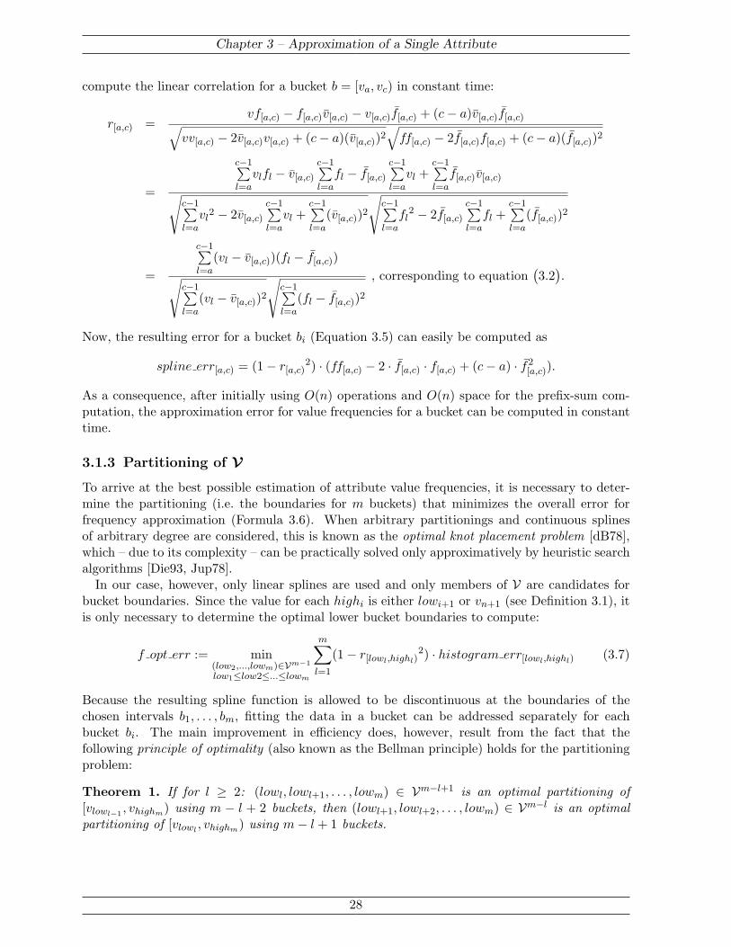
Chapter 3 – Approximation of a Single Attribute
compute the linear correlation for a bucket b = [va, vc) in constant time:
r[a,c) =vf[a,c) − f[a,c)v[a,c) − v[a,c)f[a,c) + (c− a)v[a,c)f[a,c)√
vv[a,c) − 2v[a,c)v[a,c) + (c− a)(v[a,c))2√
ff[a,c) − 2f[a,c)f[a,c) + (c− a)(f[a,c))2
=
c−1∑l=a
vlfl − v[a,c)
c−1∑l=a
fl − f[a,c)
c−1∑l=a
vl +c−1∑l=a
f[a,c)v[a,c)
√c−1∑l=a
vl2 − 2v[a,c)
c−1∑l=a
vl +c−1∑l=a
(v[a,c))2√
c−1∑l=a
fl2 − 2f[a,c)
c−1∑l=a
fl +c−1∑l=a
(f[a,c))2
=
c−1∑l=a
(vl − v[a,c))(fl − f[a,c))√
c−1∑l=a
(vl − v[a,c))2√
c−1∑l=a
(fl − f[a,c))2, corresponding to equation
(3.2
).
Now, the resulting error for a bucket bi (Equation 3.5) can easily be computed as
spline err[a,c) = (1− r[a,c)2) · (ff[a,c) − 2 · f[a,c) · f[a,c) + (c− a) · f2
[a,c)).
As a consequence, after initially using O(n) operations and O(n) space for the prefix-sum com-putation, the approximation error for value frequencies for a bucket can be computed in constanttime.
3.1.3 Partitioning of VTo arrive at the best possible estimation of attribute value frequencies, it is necessary to deter-mine the partitioning (i.e. the boundaries for m buckets) that minimizes the overall error forfrequency approximation (Formula 3.6). When arbitrary partitionings and continuous splinesof arbitrary degree are considered, this is known as the optimal knot placement problem [dB78],which – due to its complexity – can be practically solved only approximatively by heuristic searchalgorithms [Die93, Jup78].
In our case, however, only linear splines are used and only members of V are candidates forbucket boundaries. Since the value for each highi is either lowi+1 or vn+1 (see Definition 3.1), itis only necessary to determine the optimal lower bucket boundaries to compute:
f opt err := min(low2,...,lowm)∈Vm−1
low1≤low2≤...≤lowm
m∑
l=1
(1− r[lowl,highl)2) · histogram err[lowl,highl) (3.7)
Because the resulting spline function is allowed to be discontinuous at the boundaries of thechosen intervals b1, . . . , bm, fitting the data in a bucket can be addressed separately for eachbucket bi. The main improvement in efficiency does, however, result from the fact that thefollowing principle of optimality (also known as the Bellman principle) holds for the partitioningproblem:
Theorem 1. If for l ≥ 2: (lowl, lowl+1, . . . , lowm) ∈ Vm−l+1 is an optimal partitioning of[vlowl−1
, vhighm) using m − l + 2 buckets, then (lowl+1, lowl+2, . . . , lowm) ∈ Vm−l is an optimalpartitioning of [vlowl
, vhighm) using m− l + 1 buckets.
28

Chapter 3 – Approximation of a Single Attribute
Proof: Because (lowl, lowl+1, . . . , lowm) is optimal, it minimizes
E :=m∑
i=l−1
spline err[lowi,highi) = spline err[lowl−1,highl−1) +m∑
i=l
spline err[lowi,highi).
Now assume that (lowl+1, . . . , lowm) is not optimal, i.e. there exists a partitioning(low′l+1, . . . , low
′m) with
∑mi=lspline err[low′i,high′i) <
∑mi=lspline err[lowi,highi). But then
(lowl, . . . , lowm) is not optimal either, for the partitioning (lowl, low′l+1, low
′l+2, . . . , lowm) re-
sults in the overall error E′ = spline err[lowl−1,highl−1) +∑m
i=l spline err[low′i,hig′hi) < E.
Because of this property, the problem of finding an optimal partitioning can be formulated asa dynamic programming problem [Sni92]. To do this, I first formulate a recursive redefinition ofFormula 3.7. Define
f opt errhigh,m := the optimal overall error for fitting [v1, vhigh) by m buckets.
Trivially, f opt errhigh,1 = spline err[1,high). Because of Theorem 1, the error for the optimalfitting over multiple buckets can be computed as
f opt errhigh,m = minl∈{1,2,...,high}
f opt errl,m−1 + spline err[l,high]. (3.8)
Then the overall error produced by the optimal partitioning is
f opt errn,m = minl∈{1,2,...,n}
f opt errl,m−1 + spline err[l,n].
Computing the optimal partitioning
Using the above definition, the optimal partitioning of V can be computed in the followingway: f opt errhigh,m is computed for all m = 1, . . . , m (outer loop) and high = 1, . . . , n + 1(see Algorithm 1)2; these intermediate results are stored. Note that this means,that by solvingthe partitioning problem for m buckets, the solution for any number of buckets less than m isalso computed at no additional cost. Each computation requires finding the minimum among ivalues, each of which can be computed in constant time. Because the intermediate results arestored, this requires O(n) operations. Therefore the overall running time is O(m · n2) and thecomputation requires O(m) storage (the values for f opt err1,m . . . , f opt errn,m can be droppedonce m becomes greater than m + 1).
The computation of each f opt errhigh,m can be further sped up by using the idea proposedin [JKM+98] to prune the search space through the use of upper bounds for the values of f opt err.To do this, an upper bound S0 for the size of f opt errhigh,m is used. S0 can be obtained bycomputing the error corresponding to an equi-width partitioning, where all buckets are chosenso that they cover intervals of roughly the same size. This error can be computed in O(j)steps. When now computing f opt errhigh,m as defined in Equation 3.8, by iterating over allpossible values of l, all values of l for which spline err[l,high) > S0 can be ignored, as they cannotresult in an optimal partitioning. To this end the largest value for l is initially located (usinga binary search), such that spline err[l,high) > S0, which is referred to as l0. When computingf opt errhigh,m, it is now sufficient to consider only values above l0 for l, thereby improvingperformance.
2In all algorithms I have ignored the special case occurring if n < 2m. In this case there is sufficient storage spaceto store T directly and thus no approximation is necessary.
29
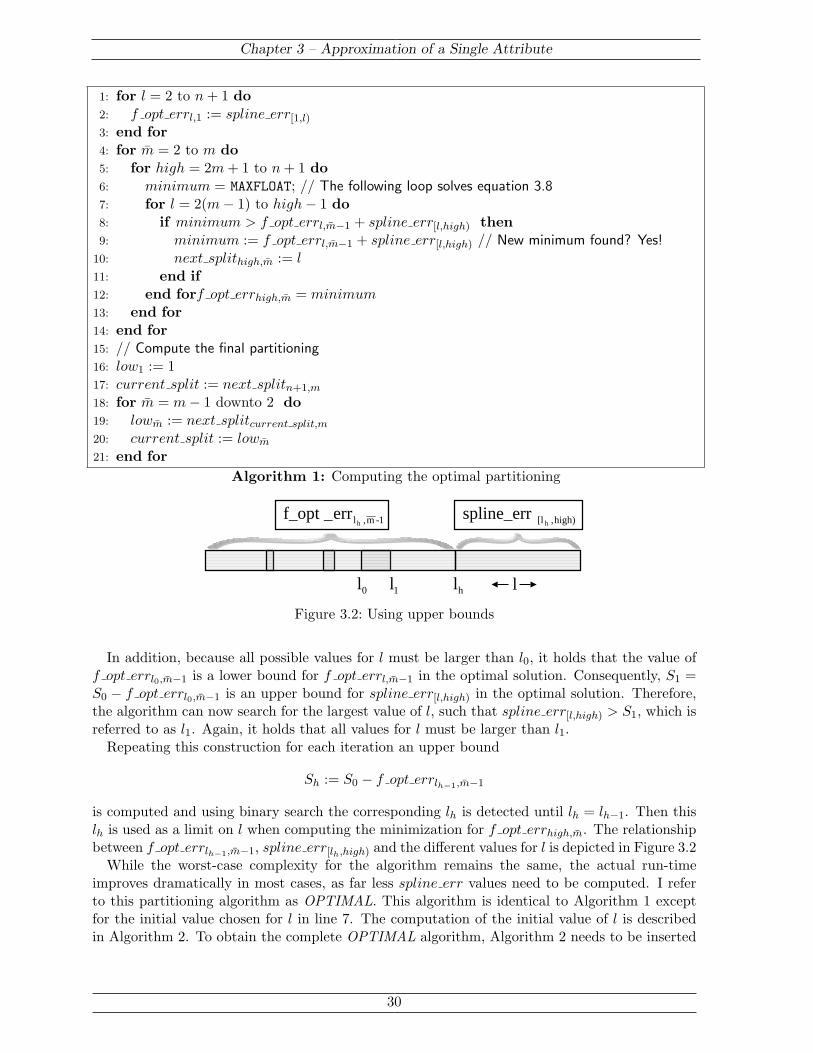
Chapter 3 – Approximation of a Single Attribute
1: for l = 2 to n + 1 do2: f opt errl,1 := spline err[1,l)
3: end for4: for m = 2 to m do5: for high = 2m + 1 to n + 1 do6: minimum = MAXFLOAT; // The following loop solves equation 3.87: for l = 2(m− 1) to high− 1 do8: if minimum > f opt errl,m−1 + spline err[l,high) then9: minimum := f opt errl,m−1 + spline err[l,high) // New minimum found? Yes!
10: next splithigh,m := l11: end if12: end forf opt errhigh,m = minimum13: end for14: end for15: // Compute the final partitioning16: low1 := 117: current split := next splitn+1,m
18: for m = m− 1 downto 2 do19: lowm := next splitcurrent split,m
20: current split := lowm
21: end forAlgorithm 1: Computing the optimal partitioning
high),[l hspline_err
l
1-m,lherr_f_opt
0l 1l hl
Figure 3.2: Using upper bounds
In addition, because all possible values for l must be larger than l0, it holds that the value off opt errl0,m−1 is a lower bound for f opt errl,m−1 in the optimal solution. Consequently, S1 =S0 − f opt errl0,m−1 is an upper bound for spline err[l,high) in the optimal solution. Therefore,the algorithm can now search for the largest value of l, such that spline err[l,high) > S1, which isreferred to as l1. Again, it holds that all values for l must be larger than l1.
Repeating this construction for each iteration an upper bound
Sh := S0 − f opt errlh−1,m−1
is computed and using binary search the corresponding lh is detected until lh = lh−1. Then thislh is used as a limit on l when computing the minimization for f opt errhigh,m. The relationshipbetween f opt errlh−1,m−1, spline err[lh,high) and the different values for l is depicted in Figure 3.2
While the worst-case complexity for the algorithm remains the same, the actual run-timeimproves dramatically in most cases, as far less spline err values need to be computed. I referto this partitioning algorithm as OPTIMAL. This algorithm is identical to Algorithm 1 exceptfor the initial value chosen for l in line 7. The computation of the initial value of l is describedin Algorithm 2. To obtain the complete OPTIMAL algorithm, Algorithm 2 needs to be inserted
30

Chapter 3 – Approximation of a Single Attribute
between lines 6 and 7 in Algorithm 1 and the final value for lh used as the lower bound for theloop in line 7.
1: // Compute S0
2: S0 := 03: width = (high− 1)/m4: for i = 0 to m− 1 do5: S0 := S0 + spine err[1+i·width,1+(i+1)·width)
6: end for7: h := 08: repeat9: // Now compute the lh corresponding to Sh
10: left := 111: right := high− 212: while right ≥ left do13: mid := (left + right)/214: if spline errmid,high > Sh then15: left := mid + 116: else17: right := mid− 118: end if19: end while20: lh := right · [spline errleft,high ≤ Sh] + left · [spline errleft,high > Sh]21: h := h + 122: Sh := S0 − f opt errlh−1,m−1
23: until lh = lh − 1
Algorithm 2: Computing the initial value for l
Greedy Partitioning
Despite the above improvements, the cost for computing an optimal partitioning could still beunacceptable when n is large. In these cases, a greedy method for the partitioning of V can beused, which results in a partitioning that is close to optimal while being much more efficient.This algorithm first partitions V into n/2 trivial bucket and then merges the ones that lead tothe smallest increase in the overall error, until only m buckets are left (see Algorithm 3). Here,the increase in the error by merging two buckets b1 = [va, vb), b2 = [vb, vc) is denoted as
error[a,b),[b,c) := spline err[a,c) − (spline err[a,b) + spline err[b,c)).
The algorithm consists of 2 loops; the for loop has n/2 iterations in which the error of mergingthe trivial buckets is computed, which can be done in constant time. The repeat loop is executed(n/2) −m times (each repetition reduces the number of buckets by one, there are n/2 bucketsinitially, and m upon termination), and executes 4 different types of operations:
1. Removing an item from the priority queue Q. An implementation of priority queues basedon Fibonacci heaps [MNU97] is used in the algorithm, allowing the removal of an item in aqueue of size n in O(log2 n) time.
2. Merging two buckets, requiring constant time.
31

Chapter 3 – Approximation of a Single Attribute
1: Partition V into n2 buckets bi = [v2i−1, v2i+1).
2: for l = 0 to n2 do
3: Compute the error[2l−1,2l+1),[2l+1,2l+3) resulting from merging the buckets bl and bl +1 andinsert the error value into priority queue Q.
4: end for5: repeat6: Remove the minimal error[a,b),[b,c) from Q.7: Merge the buckets corresponding to [a, b) and [b, c).8: Remove error[a′,a),[a,b), error[b,c),[c,c′) from Q.9: Calculate the error of joining the new bucket with its left and right neighbor (if these exist);
insert the resulting error[a′,a),[a,c), error[a,c),[c,c′) into Q.10: until there are only m buckets left.
Algorithm 3: GREEDY-MERGE
3. Calculating the error resulting from a merge, requiring constant time.
4. Inserting an item into Q, again requiring O(log2 n) time.
Since each operation is carried out no more than three times, computing a greedy partitioning isof complexity O(n log2 n). The algorithm requires O(n) storage. By performing additional m−1merge operations (i.e., until only one bucket remains), the greedy partitionings for all numbersof buckets less than m is obtained at very low additional cost. I will refer to this algorithm asGREEDY-MERGE .
In addition, I consider a second greedy partitioning-algorithm (see Algorithm 4, which takesthe opposite approach: Initially, all tuples are grouped in one bucket. Then the split that leadsto the greatest reduction in the overall error (formula 3.6) is computed and executed, resulting inan additional bucket. This is repeated, until (after m−1 splits) m buckets remain. Each time thelocation of a split is computed, at most O(n) possible split-locations need to be considered. Thesesplits are then stored in a priority queue holding at most m− 1 values (as only one split-locationis stored for each bucket). Thus the inner loop (lines 12-35) of the algorithm require O(n · log2 m)overhead. The loop itself is repeated O(m) times, and lines 1-11 compute the optimal splitlocation in the initial bucket (O(n) operations). Consequently, the overall algorithm requiresO(m · n log2 m) time and O(n) space. Like the optimal partitioning, the greedy partitionings ofV for less that m buckets are computed at no additional cost. I will refer to this algorithm asGREEDY-SPLIT .
3.2 Approximation of the Value Density
Accurate approximation of the density distribution is of critical importance for the estimation ofall queries involving grouping and aggregation. Therefore, the value densities in V are approxi-mated in addition to and independently of the value frequencies, such that:
1. the approximation captures the same number of values as V (although it should require lessvalues to represent V) and
2. the squared deviation between the actual attribute values vl ∈ V and their approximatedcounterparts vl is minimized.
32

Chapter 3 – Approximation of a Single Attribute
1: all buckets := ∅2: Insert b = [v1, vn+1) into all buckets3: minimum :=MAXFLOAT4: // Find the optimal split for the initial bucket5: for i = 3 to n− 1 do6: if minimum > error[1,i)[i,n+1) then7: minimum := error[1,i)[i,n+1)
8: min index := i9: end if
10: end for11: Insert the tuple (minimum,min index) into the priority queue Q12: for i = 3 to m do13: Remove the tuple (min, ind) from Q with the smallest min14: Remove the corresponding bucket b′ = [vlow, vhigh) with low < min < high from
all buckets15: Insert bleft = [vlow, vind) and bright = [vind, vhigh) into all buckets16: if i 6= m then17: // Find the optimal split for the new buckets18: minimum :=MAXFLOAT19: for i = low + 1 to ind− 1 do20: if minimum > error[low,i)[i,ind) then21: minimum := error[low,i)[i,ind)
22: min index := i23: end if24: end for25: Insert the tuple (minimum,min index) into the priority queue Q26: minimum :=MAXFLOAT27: for i = ind + 1 to high− 1 do28: if minimum > error[ind,i)[i,high) then29: minimum := error[ind,i)[i,high)
30: min index := i31: end if32: end for33: Insert the tuple (minimum,min index) into the priority queue Q34: end if35: end for36: // Now all buckets contains the final buckets
Algorithm 4: GREEDY-SPLIT
Analogously to the approach for frequency distributions, V is partitioned into m′ disjointintervals which are referred to as density buckets dbi = [vdlowi , vdhighi), with dlowi and dhighi
denoting the subscripts of the values from V that constitute the bucket boundaries. Analogouslyto Formula 3.1, for all i ∈ {1, 2, . . . , m′ − 1} the partitioning requires:
dhighi = dlowi+1 and dlow1 = 1, dhighm′ = n + 1.
Note that the number of buckets, m′, can be chosen independently of the number of buckets, m,for the frequency distribution of the same attribute. Using the squared deviation of attribute
33

Chapter 3 – Approximation of a Single Attribute
values, the error within bucket dbi is
density err[dlowi,dhighi) =dhighi∑
l=dlowi
(vl − vl
)2. (3.9)
In order to estimate the value distribution within a bucket, histograms use the equi-spreadassumption [Poo97], meaning that they assume that the values are spread evenly over the bucket’swidth. This means that the j-th value in a density bucket db = [dlow, dhigh) containing D valuesis approximated as v = vdlow +(j−1) · vdhigh−vdlow
D . Thus, denoting the number of values in bucketdbi by Di, the error of the bucket becomes:
histogram density err[dlowi,dhighi) =Di−1∑
l=0
(vdlowi+l −
(vdlowi +
(l · vdhighi − vdlowi
Di
)))2
. (3.10)
Using the upper and lower values to estimate the approximate spread in buckets has the dis-advantage that even when the estimation of vdhigh and vdlow is correct3, all possible partitionconstraints do not consider the width of a bucket vdhigh − vdlow as a source parameter and thusare not capable of identifying the best partitioning with regards to attribute density estimation.To illustrate this, consider the following example:
Example 3.1: Consider the set of attribute values V = {0, 1, 7, 9, 10, 13, 15}, which is approxi-mated using a 2-bucket V-optimal(V,S) histogram. This means that the final partitioningof the value domain is based on the variance of the value spreads in the resulting buckets:
o variance :=2∑
i=1
dhighi−1∑
j=dlowi
si −(
1dhighi−dlowi
dhighi−1∑
j=dlowi
si
)
2
.
However, minimizing the overall variance does not necessarily result in the optimal es-timation of the value domain. If V is partitioned into the 2 buckets b1 = [0, 9),b2 = [9, 15) the overall variance becomes o variance1 = 33/2 and the overall estimationerror error1 := histogram density err[0,9) + histogram density err[9,15) = 145/4. Onthe other hand, the partitioning b1 = [0, 10), b2 = [10, 15) results in the overall varianceo variance2 = 18 and the overall estimation error error2 := histogram density err[0,10) +histogram density err[10,15) = 47/2. Thus o variance1 < o variance2, but error1 >error2. Similar examples can be constructed for all other combinations of partitioningconstraint, source parameter and error-function (e.g., if the linear deviation of the attributevalues is used as a measure of the density error (Equation 3.9)).
The above problem has the additional unwanted side-effect, that a density-estimation may becomeworse if it receives additional memory.
In order to minimize the error defined in Equation 3.10, the termvdhighi
−vdlowiDi
, which denotesthe “gap” between adjacent values in the approximation, is treated as a control variable, denoted∆i, whose value should be chosen optimally. Note that the best value of ∆i may be larger thanboth
vdhighi−vdlowi
Diand
vdhighi+1−vdlowiDi
if the density distribution is skewed towards values closerto the interval’s upper boundary.
3This is not necessarily the case, as histograms with the sort parameter values typically only store the highestvalue in a bucket and estimate the lowest value as the successor of the highest value contained in the previousbucket [Poo97].
34

Chapter 3 – Approximation of a Single Attribute
The formula for the resulting bucket error then is obtained from equation 3.10 by replacingvdhighi
−vdlowiDi
with ∆i:
density err[dlowi,dhighi) =Di−1∑
l=0
(vdlowi+l −
(vdlowi
+ l ·∆i
))2
. (3.11)
The parameter ∆i should be chosen such that the bucket’s error is minimized, i.e.
∂density err[dlowi,dhighi)
∂∆i= 0.
Computing the derivative and solving this equation for ∆i yields
∆i = −3−vlowiDi + vlowi(Di)2 +
Di−1∑l=1
(−2l · vlowi+l)
Di (2(Di)2 − 3Di + 1), (3.12)
and this indeed results in the minimum value for Equation 3.11.The optimal density error for a bucket can now be computed by substituting vopti into equa-
tion 3.11. The overall optimal error for the entire attribute-value density synopsis then is thesum of the errors over all buckets 1,. . . , m′:
d opt errn,m′ =m′∑
i=1
density err[dlowi,dhighi). (3.13)
Using the prefix-sums defined in Section 3.1.2 it is possible to evaluate Equation 3.12 andthus density err[dlowi,dhighi) in constant time. Therefore, finding an optimal partitioning of Vand computing the optimal values for the control parameters ∆i is mathematically equivalent tothe partitioning and per-bucket parameter fitting problem for frequency distributions that weresolved in the previous section. Thus the same dynamic programming algorithm or, alternatively,one of the greedy heuristics can be applied to compute an optimal density synopsis with a givennumber m′ of buckets. I refer to the resulting error as d opt err1,m′ .
3.3 Synopsis Storage
In the following I will describe what information is stored in the buckets used for attribute-value frequency and attribute-value density approximation and how the memory M available tothe entire synopses is divided between the two approximation types (Section 3.3.2). A similarapproach is used to divide the available memory between multiple spline synopses (Section 3.3.3).To ensure accurate estimation of value frequencies, it is also important to match up the differentapproximations to some degree, which is being discussed in Section 3.3.4.
3.3.1 Storage Requirements
The buckets for both frequency and density approximation store 3 values each. Frequency-approximation buckets store:
(a) the leftmost attribute value in the bucket, and(b) the two coefficients αi and βi.
35
Chapter 3 – Approximation of a Single Attribute
Density-approximation buckets store:
(a) the leftmost attribute value in the bucket,(b) the fitting-parameter ∆i, and(c) the number Di of unique attribute values contained in the bucket.
Assuming each value is stored using a constant length number, the storage requirements for bothbucket types are identical.
3.3.2 Reconciling Frequency and Density Synopses for One Attribute
So far I have shown how to minimize the error for each aspect separately, but assumed that thenumber of buckets, m for frequency and m′ for density synopses, is fixed and a priori given for eachsynopsis. To reconcile both synopses for an attribute, the problem is how to divide the availablememory space between them, i.e., how to choose the values of m and m′ under the constraintthat their sum should not exceed a given constant M . Intuitively, we are interested in allocatingthe memory in such a way that the aspect that is more difficult to approximate is given a highernumber of buckets. This amounts to minimizing the combined error of both approximations.However, to make sure that we do not to compare “apples with oranges” (i.e., value frequenciesversus actual data values), it has to be taken into account that the two approximations refer todomains with possibly radically different scales. Therefore, the error metrics are first normalizedfor the two classes of synopses thereby defining a relative error for each aspect. As the normalizingfactor, I use the highest possible approximation error for each domain, i.e. the maximal differencebetween the actual value fi (or vi) and it’s approximation fi (or vi, respectively), when therespective domain is approximated using one bucket only. Intuitively, these factors represent the”difficulty” of approximating each domain. I refer to these factors as f domain and v domain;the relative error for a single value vi then becomes
(vl−vl
v domain
)2 = (vl−vl)2
(v domain)2. The relative error
for a single frequency is(fj−frq(vj)
f domain
)2 = (fj−frq(vj))2
(f domain)2.
In addition to this normalization it is desirable to consider the relative importance of the twosynopses. With a query workload that is dominated by range or exact-match queries, frequencyestimations are obviously the key point. On the other hand, with a workload that requires manyestimations of the result size of projection and grouping queries, the density synopses becomemore important. This consideration will be discussed in more detail in Chapter 5 in the contextof the physical design problem for data synopses.
To divide the available memory, I exploit the fact that computing the optimal partitioningof either approximation type for j buckets, using the algorithms of Section 3.1.3, also generatesthe optimal partitionings for 1, . . . , j − 1 buckets at no additional computational cost. The sameholds for the GREEDY-SPLIT heuristics; and for GREEDY-MERGE the additional output canbe generated at very small extra cost (with j additional merge operations). Thus, with a givenamount of memory for a total of M buckets, I compute the optimal partitionings and resultingrelative errors for each approximation with up to M − 1 buckets, and then divide the availablememory in such a way that the sum of the combined relative error terms
f d err =f opt err1,m
(f domain)2+
d opt err1,m′
(v domain)2(3.14)
is minimized under the constraint that m ≥ 1, m′ ≥ 1 and m + m′ = M . This is a trivialcombinatorial problem, solvable in O(M) steps.
36

Chapter 3 – Approximation of a Single Attribute
3.3.3 Reconciling Multiple Synopses
When the overall available memory M needs to be divided between h different synopses over theattributes Ri1 .Aj1 ,. . . ,Rih .Ajh
, the sizes of the single frequency and density approximations areagain chosen in such a way that the combined relative error over all synopses is minimized. Thus,if f d errRil
.Ajldenotes the combined relative error for the approximation of attribute Ril .Ajl
,the sizes of each separate approximation is choose so that the term
overall f d errM :=h∑
l=1
f d errRil.Ajl
is minimized. Similar to the partitioning problem for V, the bellman principle holds, therebyallowing to compute the optimal memory allocation using O(h ·M2) operations. While a goodapproximative solution can again be computed using greedy heuristics, it is generally the casethat M ¿ n, and therefore the time for computing the optimal memory partitioning insignif-icant (see Section 3.5.3). Note that solving the minimization problem also gives the values foroverall f d errM for all values M ≤ M .
3.3.4 Matching Frequency and Density Synopses
While the above techniques allow us to minimize the weighted sum of the approximation error forattribute value density and frequency, this is not always sufficient to guarantee a low estimationerror for the queries described in the previous subsection.
In order to illustrate the problem, I examine a value-frequency pair (vl, fl) from a data distri-bution T and its approximation
(vl, fl
). Since frequencies are approximated as linear spline func-
tions frqi, i = 1, . . . , m over V,(vl, fl
)can be written as
(vl, frqk(vl)
)for some k ∈ {1, . . . , m}.
When approximating attribute-value frequencies, the error of Formula 3.3 is minimized andthe frequencies at the original attribute values v1, . . . , vn are fit, rather than their approxima-tions v1, . . . , vn. In most cases (when vl and vl belong to the same frequency bucket k, withfrqk(x) = αk · x + βk) this still results in accurate approximation, since the approximation error
for fl := |fl − frqk(vl)|= |fl − frqk(vl + (vl − vl))|= | fl − frqk(vl)︸ ︷︷ ︸
minimized by frequency approx
+αk · (vl − vl)︸ ︷︷ ︸minimized by density approx
|.
The problem becomes apparent either for large values of αk (resulting in a large second term inthe above formula) or when vl and vl belong to different frequency buckets. In the latter case(demonstrated in Figure 3.3), the frequency of vl is estimated as frqk(vl), whereas the frequencyof vl by frqt(vl), t 6= k. Now, frqk is chosen to fit all points in [lowk, highk), among them (vl, fl),optimally, thereby reducing the error |fl− frqk(vl)|. The function frqt is fitted to a different setof points, not including (vl, fl), and therefore a possibly poor estimator for fl.
To avoid this problem, I use T = {(v1, f1), . . . , (vn, fn)} for the approximation of the frequencydomain, thereby minimizing the approximation error for the attribute values which will laterbe used in estimation. So density is approximated first, and the frequency approximation thenuses the approximate density rather than the original distribution. However, T depends on thenumber of buckets m′ used for the approximation of the attribute value density, which in turndepends on the error f opt err1,m (see Formula 3.8) made when fitting T . A straightforwardsolution would be to compute the resulting T for all possible M − 1 values of m′, fit them, and
37

Chapter 3 – Approximation of a Single Attribute
Val
ue F
requ
ency
Attribute Valuevl
Bucket2
vl
Bucket1
frq1
�vl, frq1(vl)
�
frq2
�vl, frq2(vl)
�
Figure 3.3: The need for matching approximations
then determine the optimal combination of density and frequency error. This, however, wouldincrease the computational complexity of our approach by the factor of M . Therefore, I use asimpler approach. First, the error f opt err1,m for fitting T is computed and used to determinethe corresponding numbers of buckets, m,m′, for frequency and density approximation. Then Tis re-computed for this value for m′, which is then used to compute the optimal approximationof the value frequency, with the resulting spline being the final synopsis. Thus the optimalpartitioning of V for value frequency approximation is only computed twice, instead of M times.Furthermore, since the f opt err1,m values for fitting T and for fitting T typically close to eachother, both approaches tend to result in the same values for m and m′ and therefore in identicalapproximations.
3.3.5 Weighted Approximation
In Chapter 5 it will become necessary to solve a modified version of the approximations described,for the estimation for each value vi and frequency fi will be assigned a relative weight wi. Thismeans that the error-functions to be minimized when approximating a bucket bi = [lowi, highi)are
highi∑
l=lowi
wl(frqi(vl)− fl)2 andhighi∑
l=lowi
wl(vl − vl)2.
While this results in changes to some details for the approximation (the prefix-sums used needto be weighted as well, and the formulas for evaluating the error for a bucket in constant timechange), the computational properties and the overall approach remain the same.
3.4 Using Spline Synopses for Query Estimation
In the following I describe how to use the resulting synopses for estimating the result sizesof various types of basic queries and for approximative query answering. The focus is on thefollowing query types: projections or, equivalently as far as result-size estimation is concerned,grouping with aggregation, range queries on a single attribute, and joins, with projections andjoins possibly restricted to a specified value range (i.e., in conjunction with a range filter). Theextension to complex operator-trees is then straightforward: the initial approximate query-resultsat every branch of the operator tree are then subjected to the further operators using the operatorsemantics described in Section 2.2.
Because the estimation of join queries is inherently difficult when using synopses for the twojoining relations only (independent of which approximation technique is used ), special join
38
Chapter 3 – Approximation of a Single Attribute
synopses are introduced, which provide additional information on the number and value of theattribute values that find join-partners in the two relations.
3.4.1 Projections (and Grouping Queries)
When estimating the (number of) unique values resulting from a projection over the interval[a, b), there are three cases to differentiate:
• If [a, b) corresponds to the boundaries of a density bucket dbi (i.e., a = vdlowi and b =vdlowi+1), the resulting value distribution is
V :={
vdlowi+ l ·∆i
∣∣∣l = 0, . . . , Di − 1}
.
If only the size of the query result is of interest, the estimation corresponds to the numberof values in bucket i:
P i[a,b) = Di.
The notation P i[a,b) is used to indicate that the query over [a, b) is answered using only
bucket i.
• If [a, b) is completely contained in density bucket dbi (i.e., a ≥ vdlowi and b < vdlowi+1), theresulting value distribution is computed analogously, the only difference being that onlyvalues between a and b are considered:
V :={
vdlowi + l ·∆i
∣∣∣l =⌈
a−vdlowi∆i
⌉, . . . ,
⌊b−vdlowi
∆i
⌋}.
Again, when only the result size is of interest, the estimation returns only the number ofunique values occurring in V:
P i[a,b) =
⌈b−vdlowi
∆i+ 1
⌉−
⌊a−vdlowi
∆i
⌋.
• Finally, an approximate projection query for [a, b) that spans more than one density bucketcan easily be estimated by clipping [a, b) against the buckets and building the union of theestimations for the intervals [a, vdlowj ), [vdlowj , vdlowj+1), . . . [vdlowj+l
, b). Thus, the estima-tion problem is reduced to the previous formulas.
Consequently, any projection query requiring the approximation of an approximate value distri-bution V can be estimated using O(|V|) operations. If only the result size is of interest, it can beestimated using O(m′) operations. Whenever approximating values over discrete value domains(e.g., integer domains), one can improve the estimation quality by rounding to the next discretevalue.
3.4.2 Range Selections
For purpose of range selections, it is first necessary to introduce a unified notation for the splinefunctions frq1, . . . , frqm that approximate the frequency distribution.
Definition 3.1 (Frequency Approximation Function) :The frequency approximation function described through the attribute frequency approxi-mation of an attribute Ri.Aj is a mapping frequencyRi.Aj : DRi.Aj 7→ N defined by
frequencyRi.Aj (x) :=m∑
l=1
frql(x) · [lowl ≤ x < highl].
39
Chapter 3 – Approximation of a Single Attribute
If the result it not in N, it is rounded to the next integer. When it is clear, which relationand attribute are referred to, the subscript Ri.Aj is dropped.
To estimate the query result for a range query with range [a, b), first the approximative den-sity distribution V is computed for [a, b) using the above technique for projection queries (seeSection 3.4.1), and then the frequency distribution of the range query result is computed asF = {frequency(v) | v ∈ V}.
When only the number of tuples in [a, b), i.e., the query result size, is to be estimated, thecomputation can be sped up in the following way. Here, it is necessary to differentiate two cases:
• The interval [a, b) is completely contained in a density bucket dbi (i.e., a ≥ vdlowi andb ≤ vdlowi+1).In this case, the estimation of the result size requires the evaluation of mterms, with m corresponding to the number of buckets bl, . . . , bl+m−1 (used for frequencyestimation) that intersect the interval [a, b). For these buckets I now estimate the numberof tuples in the corresponding intervals [a, vlowl+1
), [vlowl+1, vlowl+2
), . . . , [vlowl+m−1, b). For
each interval I = [start, end) that corresponds to the intersection of density-bucket dbi andfrequency-bucket bj , the number of tuples is estimated as
Si,j[start,end) : =
bend−vdlowi/∆ic∑
l=dstart−vdlowi/∆ie
frqj
(vdlowi
+ l ·∆i
)(3.15)
=(⌈
end−vdlowi∆i
⌉−
⌊start−vdlowi
∆i
⌋+ 1
)(βj + αj · vdlowi)
+∆iαj
2
(⌈end−vdlowi
∆i
⌉−
⌊start−vdlowi
∆i
⌋+ 1
)(⌈end−vdlowi
∆i
⌉−
⌊start−vdlowi
∆i
⌋).
The importance of the second equality is that it means Si,j[start,end) can be evaluated in
constant time. The estimation over [a, b) can now be computed as
Si[a,b) := Si,j
[a,vlowl+1) +
(l+m−2∑
h=l+1
Si,h[vlowh
,vlowh+1)
)+ Si,l+m−1
[vlowl+m−1,b),
requiring O(m) operations.
• When interval [a, b) spans multiple density-buckets the estimation problem can be reducedto the previous formulas by clipping [a, b) against the buckets and building the union of theestimations for the intervals [a, vdlowj ), [vdlowj , vdlowj+1), . . . [vdlowj+l
, b). Then the selectivitycan be computed as
S[a,b) := Sj[a,vdlowj
+( l−1∑
h=1
Sj+h[dlowj+h,dlowj+h+1)
)+ Sj+l
[dlowj+l,b). (3.16)
For all intervals [start, end) for which the term 3.15 is evaluated the values for start, endcome from the set
Bounds := {max{start, vlow1}, vlow2 , . . . , vlowm , vdlow2 , . . . , vdlowm′ , min{end, vn+1}}
with @middle ∈ Bounds ∴ start < middle < end (otherwise the intervals [start, middle)and [middle, end) would be evaluated instead). Because there are only m + m′ such com-binations possible, expression 3.16 can be evaluated using at most O(m + m′) evaluationsof term 3.15.
40

Chapter 3 – Approximation of a Single Attribute
Consequently, any range-selection query requiring the approximation of an approximate datadistribution V can be estimated using O(|V|) operations. If only the result size is of interest, theestimation requires O(m + m′) operations.
Because spline synopses provide query result estimation, they can be used to estimate anyfilter condition other than range-specifications as well.
3.4.3 The Inherent Difficulty of Join Estimation
In principle, the data synopses constructed so far can also be used when estimating a joinquery between two relation R1 and R2: first the approximative density distributions V1 andV2 would be computed and the join between them would be performed, resulting in the approx-imate density distribution Vjoin. The join result’s frequency distribution would be computed asFjoin = {frequency1(v) · frequency2(v) | v ∈ Vjoin}, with frequency1 and frequency2 being thefrequency functions of the two join attributes.
This approach is similar to how joins are estimated by histograms and in [CGRS00] (the onlytechniques besides spline synopses capable of both query result and join estimation) in thatfirst a join is performed on the approximate attribute value distribution and the frequencies ofthe values with join partners are then computed as the product of the corresponding frequencyapproximations. Unfortunately, this approach does not lead to accurate join estimation. Thereason for this is that even small errors incurred when approximating the attribute value domaincan lead to drastic changes in the number and value of attribute values that find a join partner4.Therefore, minimizing the average error in the approximation is not sufficient to ensure accuratejoin estimation.
Example 3.2: To illustrate this point, consider the approximation of the equi-join between twodata distributions T1 = {(v1, f1), . . . , (vn, fn)} and T2 = {(v1, f
′1), . . . , (vk, f
′k)} via spline
synopses. Assume that T1 is approximated exactly. If the approximation of the attributedensity of T2 has very low error, but is not exact, i.e., at least a single value vi and itsapproximation vi differ by more than 1, then it will not find its correct join-partner. Incase it does not find a join-partner at all (i.e. @j ∈ {1, . . . , n} : vi = vj , the join is thenunderestimated by at least fi · f ′i .
The same problem exists for histograms, especially since most histogram types are geared towardsminimizing the estimation error for attribute value frequency only. To limit the estimation errorwhen either fi or f ′i are very large, high-biased [IP95] and various kinds of end-biased [Poo97]histograms have been proposed, which keep the attribute values with the highest (and in the caseof end-biased histograms also the lowest) frequencies in singleton buckets storing only a singleattribute value. Thereby, these attribute values and frequencies are estimated correctly. Still,this approach fails whenever an attribute value involved in a join is not in a singleton bucket forboth histograms. Especially in foreign-key joins, where all values are keys in one of the joiningrelations and thus only have frequency 1, most high-frequency tuples in the joining relation tendto be matched up with tuples not in singleton buckets.
Example 3.3: To illustrate that the same problem arises also for join estimation via wavelets,consider the following example:
T1 = {(v1, 2), (v2, 0), (v3, 7), (v4, 2)} T2 = {(v1, 10), (v2, 10000), . . .}4The only exception to this are scenarios involving band-joins [DaJB93] with sufficiently large sizes of the band
interval.
41

Chapter 3 – Approximation of a Single Attribute
Even if the approximation keeps all coefficients necessary to represent T2 and dropsonly a single coefficient of the representation of T1, the approximation of the joinbetween the two distributions exhibits a large error, for the approximation T1 ={(v1, 1), (v2, 1), (v3, 7), (v4, 2)} now joins the 10000 T2 tuples with value v2. The reasonfor this phenomenon is the fact that the thresholding scheme employed in [CGRS00] mini-mizes the overall mean squared error
∑Ti=1(fi− fi)2 for each relation, which minimizes the
error regarding range selection queries, but disregards accurate join estimation.
In general, regardless of which data approximation technique is used, it holds that it is not fea-sible to estimate arbitrary join queries from approximations of the joining base relations withacceptable accuracy. This phenomenon was first discussed extensively in [CMN99] in the contextof sampling:
Theorem [CMN99]: Assume the samples S1, S2 of two joining attributes R1.A1, R2.A2, with S1
sampling the fraction 1/ε1 of R1, and S2 sampling the fraction 1/ε2 of R2. Both samples do notcapture the entire data distribution, i.e. ε1 > 1 and ε2 > 1. Then it is not possible to generate asample of the join R1
A1=A2./ R2 for any fraction 1/εj > 0 from S1, S2.
A similar result can be formulated for all other estimation technqiues as well. In the case ofspline synopses it holds that
Theorem 2. Given two synopses over two relations R1.A1, R2, A2, approximating data distri-butions T1 = {(v1, f1) . . . , (vn, fn)}, T2 = {(v′1, f ′1) . . . , (vk, f
′k)} with the attribute value domain
being N and rounding used in estimation. Assume that T1 is captured exactly by a spline synopsis.Further assume that the attribute frequency approximation for T2 is exact, and the attribute den-sity approximation has error d opt err1,m′ ≤ (min{n, k}), with m′ being the number of bucketsused in the density approximation for T2. Then the estimation of the number of values that finda join partner may be off by no match := min{n, k} −m′, potentially resulting in an error forestimating the number of tuples in the join result of
join error max := maxi1,...,ino match∈{1,...n}
∀t∈{1,...,no match−1}:it<it+1
max
l1,...,lno match∈{1,...k}∀t∈{1,...,no match−1}:it<it+1
no match∑
j=1
fij · f ′lj
.
(3.17)
Proof: To show this, I first illustrate how to construct example data distributions T1, T2 for agiven number of buckets m′ used in density approximation for T2 so that the join-estimation erroris equal to the one stated in Term 3.17. Then I show that this term constitutes an upper boundfor the join error, i.e., that it is not possible to construct distributions resulting in greater joinerror.Let T2 = {(v′1, f ′1) . . . , (vk, f
′k)} with k = 3 ·m and the attribute values defined as follows:
for l = 0, . . .m′ − 1 : v′3l+1 = 4l · k, v′3l+2 = v′3l+1 + 1, v′3(l+1) = v′3l+1 + 5
Consequently, the final partitioning always groups the values v′3l+1, . . . , v′3(l+1) in a single bucket
(otherwise there is a least one bucket containing values v′3l+1, v′3l and either v′3l+2 or v′3l−1 for
some l ∈ {l = 1, . . .m′ − 1}, resulting in an estimation error of d opt err1,m′ ≥ (k)2; thus, this isnot the optimal partitioning).
42
Chapter 3 – Approximation of a Single Attribute
This partitioning results in an error of less than 2 per bucket and thus d opt err1,m′ ≤ (k)and the value for the fitting parameter ∆i = 1.8 for any bucket. Therefore the approximationv′i, i = 1, . . . , k of the attribute values has the following properties:
for l = 0, . . . m′ − 1 : v′3l+1 = v′3l+1, v′3l+2 = v′3l+2 − 1, v′3(l+1) = v′3(l+1) − 1.
So out of three values in each bucket, only the first is approximated correctly. Now choose thefrequencies f ′i , i = 1, . . . , k in T2 in such a way, that for fi = 1 for all i mod l = 1 (i.e. thecorresponding value is approximated exactly), and fi > 1 otherwise. The the 2m′ = min{k, n}−m′ values that are not estimated exactly do not find a join partner when estimating the join.
Finally, define T1 := {(v′1, f ′1), . . . , v′k, f ′k} (i.e. identical to T2); then the attribute values corre-sponding to the min{k, n}−m′ largest frequency join with each other. So the join is estimated asjoin estimate = k/3 with the real size being join exact = k/3 + join error max. Analogously,if T1 is defined as T1 = {(v′1, f ′1), . . . , v′k, f ′k} the estimated join size is k/3 + join error max andthe correct result size k/3.
On the other hand, the join error cannot grow beyond the value of Term 3.17, when thefrequency distribution is captured correctly. This is due to the fact that no matter how largethe error for value density estimation, the smallest values in each bucket are always estimatedcorrectly. As a consequence, in the above example at least m′ values find the correct join partner.Therefore the estimation of the number of values that find a join partner may be off by min{k, n}−m′ at most and thus the overall error for estimating the result size is limited to the min{k, n}−m′
largest combinations of frequencies.
The key result here is that the estimation error for join estimation is not limited directly by(a function of) the estimation error for the attribute frequencies or attribute densities, i.e., itis not possible to formulate an upper bound for the join error join error max of the naturejoin error max ≤ g(f opt errn,m, d opt errn,m′) for some function g. For this reason, I nowintroduce join-synopses dedicated to capturing the distributions present in the join result, therebylimiting the error for join-estimation. Through these join synopses it is then possible to limitthe join-estimation error by limiting the estimation error for value frequency and value densityestimation.
3.4.4 Join Synopses
In order to provide accurate estimation for equi-joins and also other types of joins, I extendthe idea proposed in [APR99] for sampling to capture join-result distributions in a special classof join synopses. This approach is feasible because there is typically only a small number ofattribute combinations (when compared to the number of all possible attribute combinations)that are used in join-operations. Therefore, the number of additional join synopses typically isof cardinality similar to the number of synopses itself.
There are two types of join synopses: join density synopses, which approximate the distributionattribute values common to both join attributes and thus present in the join themselves (with thecorresponding frequencies computed via the base relations) and full join synopses which capturethe frequency distribution of the join as well.
Definition 3.2 (Join Density Synopses) :
A join density synopsis for the join R1A1=A2
./ R2 is an attribute density approximation ofthe set J = {v1, . . . , vl} of values that are present in both the data distribution of R1.A1
and that of R2.A2.
43

Chapter 3 – Approximation of a Single Attribute
When estimating a join R1A1=A2
./ R2 query using a join density synopsis, initially the approx-imate value distribution J = {v1, . . . , vl} is computed. Then the value frequencies are computedusing the frequency functions frequencyR1.A1 , frequencyR2.A2 (see Section 3.4.2) described bythe spline functions used to approximate the frequency distributions of the joining attributes:
F = {frequencyR1.A1(v) · frequencyR2.A2(v) | (v) ∈ (J )}.As a result, the worst-case error for join estimation is reduced significantly.
Theorem 3. Given two synopses over two relations R1.A1, R2.A2 which approximate the datadistributions T1 = {(v1, f1) . . . , (vn, fn)}, T2 = {(v′1, f ′1) . . . , (vk, f
′k)} with the attribute value do-
main being N and rounding used in estimation. Then the subscripts of the joining values in R1.A1
and R2.A2 are I = {(i, j) | vi = v′j , i ∈ {1, . . . n}, j ∈ {1, . . . k}}.Consider the set of values finding a join partner J = {vi | ∃j ∈ {1, . . . k} : (i, j) ∈ I}.
When R1A1=A2
./ R2 is estimated using a join density synopsis approximating J ⊆ VR1.A1 asJ = {vl1 , . . . , vl|J |}, the largest possible error is the size of the join estimation can be describedas
join error max :=∑
(i,j)∈I|frequency1(vi) · frequency2(vi)− fi · f ′j |. (3.18)
Proof: The size of the join result R1A1=A2
./ R2 is the sum of the product of the frequencies of thevalues finding a join-partner: join size :=
∑(i,j)∈I fi · f ′j . The size of its estimation is then the
estimation of the above sum join size est :=∑
(i,j)∈I frequency1(vi)·frequency2(vi). If the esti-mation of all the frequencies in the join result are either over- or underestimated (i.e., ∀(i, j) ∈ I :fi · f ′j ≥ frequency1(vi) · frequency2(vi)∨∀(i, j) ∈ I : fi · f ′j ≤ frequency1(vi) · frequency2(vi)),the difference |join size− join size est| is equal to Term 3.18.
Thus, the join estimation error results from inaccuracies in the attribute frequency approximationonly. The error in join size estimation is bounded by the sum of the errors in estimation of thefrequency approximation for all frequencies f join
i,j = fi · f ′j present in the join result.However, the above formulation conceals one additional problem: while join density synopses
result in correct estimation of the number of joining attribute values (over the entire value do-main), the fact that the frequencies present in the join result are estimated through the frequencyapproximation of the base relation results in the matching problem discussed for range-selectionqueries in Section 3.3.4. Unlike the case of the matching problem for range-selection queries,using the approximate attribute values as additional points for the spline-fitting problem is notpossible without making the frequency approximation more difficult, for the approximate valuesin the approximation of joining tuples J are not necessarily a subset of the approximate values inthe approximation of the attribute density V for either relation. Thus, for every join considered inthe fitting of value frequencies, the number of values for which the fitting is computed potentiallyincreases by |J |, significantly increasing the resulting overhead and decreasing the accuracy ofthe resulting frequency approximation.
This problem can be avoided by separating the approximation of frequencies in the base rela-tions from the frequency approximation for the join result.
Definition 3.3 (Full Join Synopses) :
A full join synopsis for a join R1A1=A2
./ R2 is an approximation of the data distributionTJ = {(v1, f1), . . . , (vl, fl)} of the join result. It includes both attribute frequency anddensity approximation.
44

Chapter 3 – Approximation of a Single Attribute
Theorem 4. Given two synopses over two relations R1.A1, R2.A2 which approximate the datadistributions T1 = {(v1, f1) . . . , (vn, fn)}, T2 = {(v′1, f ′1) . . . , (vk, f
′k)} with the attribute value do-
main being N and rounding used in estimation. Then the subscripts of the joining values areI = {(i, j) | vi = v′j , i ∈ {1, . . . n}, i ∈ {1, . . . k}}.
Consider the set of values finding a join-partner J = {vi | ∃j ∈ {1, . . . k} : (i, j) ∈ I}. Thus the
data distribution of the join result is TJ = {(vi, fi,j) | (i, j) ∈ I∧fi,j = fi ·f ′j}. When R1A1=A2
./ R2
is estimated using a full join synopsis approximating TJ as TJ = {(vi, fi,j) | (i, j) ∈ I}, the largestpossible error for the join size estimation is
join error max :=∑
(i,j)∈I|fi,j − fi · f ′j |. (3.19)
Proof: This proof is analogous to the one of Theorem 3. The size of the join result R1A1=A2
./ R2
is the sum of the product of the frequencies of the values finding a join-partner: join size :=∑(i,j)∈I fi ·f ′j . The size of its estimation is then the sum of the approximate frequencies in the ap-
proximation of TJ : join size est :=∑
(i,j)∈I fi,j . If the estimation of all the frequencies in the joinresult are either over- or underestimated (i.e., ∀(i, j) ∈ I : fi ·f ′j ≥ fi,j∨∀(i, j) ∈ I : fi ·f ′j ≤ fi,j ,the difference |join size− join size est| is equal to Term 3.19.
Because of the drawbacks of density join synopses discussed above, I only consider full joinsynopses in the following sections.
The overall drawback of using additional join synopses is that they compete for the limitedmemory reserved for synopses overall. Thus, by creating and storing additional join synopses,the quality of frequency and density approximation is reduced elsewhere. For this reason, joinsynopses should only be constructed in cases, where “normal” join estimation as described aboveis sufficiently inaccurate to justify the required space. In the following (Section 3.4.5), I introducea self-tuning algorithm which computes join synopses only in this case. To assess the error for joinestimation for query result estimation, it is necessary to define a new error metric (Section 3.4.4).Based on the values of this error the algorithm then chooses for which joins to construct joinsynopses and chooses their sizes (Section 3.4.5). Finally, the improvement resulting from thisapproach and the different types of join synopses is evaluated (Section 3.4.6).
Computing the Join Error
To assess the improvement from the use of additional join synopses it is necessary to define anerror metric for a join estimation, i.e., the error between a join result J and its approximation J .
For the purpose of selectivity estimation, it might be sufficient to use the deviation in the num-ber of tuples; however, this is not sufficient for other purposes, since the approximate join-resultmight be subject to further operations. This means that both the deviation in the individual tu-ple frequencies and the deviation in the attribute density distribution of the join-attribute valuesthat are present in the join result have to be taken into account. In addition, the approximatedand the actual join result may contain a different number of unique attribute values. A priori itis unclear how to match the values in the approximated join with the values that occur in theactual result. Simply matching the i-th value in each distribution is not satisfactory, even if Jand J contained the same number of values.
Example 3.4: To illustrate this point, consider the case where J = {(v1, f1), . . . , (vn−1, fn−1)}and J = {(v2, f2), . . . , (vn, fn)}, which would incur a large error if tuples were simply
45
Chapter 3 – Approximation of a Single Attribute
matched pairwise in the above orders, although the join result and its approximation matchperfectly except for one value.
Instead, individual tuples should be matched by their join-attribute-value distances to computethe error between the approximation and the actual result. For tractability this is done in agreedy fashion:
1. First, match all tuples of equal attribute values, i.e. all (va, fa) ∈ J, (vb, fb) ∈ J where va =vb.
2. Then, match the tuples (va, fa) ∈ J, (vb, fb) ∈ J where the distance between va and vb isminimal. This is repeated until only tuples from either J of J remain.
3. Finally ||J | − |J || unmatched tuples remain. Each is matched with an artificial value withfrequency 0, located in the center of the value set of the join attribute.
Using a merge-based approach, it is possible to compute this matching efficiently. Initially,both J and J are merged into a single list sorted by the attribute value of each tuple; in thisprocess, all exact matches are eliminated (step 1). For each matching in step 2, only the up to2 ·min{|J |, |J |} distances between tuples adjacent in the resulting list, and coming from differentsets are considered; these are stored in a priority queue [MNU97]. Each time a pair of tuples ismatched, these are eliminated from the list, and at most one new distance needs to be computed.Therefore the computational complexity of the three steps is (with p = min{|J |, |J |} and l =max{|J |, |J |}): O(p) (steps 1&3) and O(l log2 l) (step 2). All steps have to be executed once foreach possible allocation of join buckets, so if M denotes the overall number of buckets and k thenumber of different attributes in the approximation, the matching has to be carried out M −2 ·ktimes, resulting in the overall complexity of O((M − k) · (p + l log2 l)).
Once this matching is obtained, the overall error is computed analogously to the error forfrequency and density distributions, namely, by computing the relative difference in valueand frequency for each matching pair of tuples. The normalizing factors f join domain andv join domain are computed as before (see Section 3.3.2).
join error :=∑
all matched tuples (a,b)
(va−vb
v join domain
)2+
(fa−fb
f join domain
)2
+∑
all unmatched tuples q in J
(vq−(v|J|−v0)/2
v domain
)2+
(fq−0
f join domain
)2
+∑
all unmatched tuples q in J
(vq−(v|J|−v0)/2
v domain
)2+
(fa−0
f join domain
)2
3.4.5 Integrating Join Synopses
Join synopses have been shown to limit the worst-case estimation error for join-queries; still,because they compete for the memory used by spline synopses, they should only be added, whenthe estimation of the corresponding join improves significantly through this. Integrating dedicatedjoin synopses for selected equijoins again means solving the problem of how to divide memorybetween the approximations over all synopses. In the following, I explain how to determinewhether a join synopsis for a particular equijoin Ri
Ac=Ad./ Rj should be included and how many
buckets this join synopsis receives. As before, I assume that there is memory for a total of Mbuckets. Further, let Vjoin denote the density distribution of the join result.
46

Chapter 3 – Approximation of a Single Attribute
Assuming that the problem of dividing up the memory for the density and frequency synopsesfor all k attributes (see Section 3.3.3) is solved already. This means that the optimal partitioningfor each attribute and corresponding errors for all numbers of buckets (overall) less or equalto M are known. Now the error resulting from estimating the join using no additional joinsynopsis is computed. For this purpose, I compute the approximate join Ri
Ac=Ad./ Rj using the
straightforward join computation described in Section 3.4.3 and then compute the resulting error,which is referred to as standard join err.
Furthermore, for l = 1, . . . ,M − 2k, the join approximation resulting from using l bucketsfor an additional join synopsis is computed as follows. For each l, the algorithm computesthe join-synopsis using l buckets, and the resulting approximate data distribution Tl. Basedon Tl, the corresponding join error is computed, which I refer to as join errl. Also, I definejoin err0 := standard join err.
Since essentially the same error metrics are used for join-result and base-data distributions,their values may be compared directly. Then, the problem of partitioning the available memoryagain means finding l such that the overall error
final syn err := overall f d errM−l + join errl is minimal.
For multiple joins, the optimization can be extended analogously to Section 3.3.3; the problemof partitioning the available memory M for k synopses and h possible joins is again a dynamicprogramming problem, requiring O(M2 · (2 · k + h)) operations.
3.4.6 Experimental Evaluation of Join Synopses
As shown in Section 3.4.4, the use of join synopses has significant impact on limiting the worst-case error for join estimation. To examine how much the use of dedicated join synopses alsoimpacts join estimation in practice, I consider the following experimental setup. Given twosingle-attribute relations R1 and R2 corresponding to the data distributions T1, T2 over the valuedomains DR1 = DR2 := {1, . . . , 100}. T1 are T2 defined so that both distribution contain 40randomly chosen values with |VR1 ∩ VR2 | = 20 (i.e., 20 values find a join partner in the equi-joinR1 ./ R2). The frequencies of the joining tuples are chosen uniformly between 10 and 50.
For these distributions, I then construct two different combinations of synopses for a givenamount of memory M :
(a) A synopsis of each T1 and T2.(b) A synopsis of T1 and T2 and a full join synopsis of R1 ./ R2.The sizes for the different synopses are chosen in such a way that the synopses for T1 and T2
have equal size (if M ÷3 is uneven, T1 receives the extra bucket) and the size of the join synopsisis computed as detailed in Section 3.4.5. I then measure the error for estimating the number oftuples in R1 ./ R2 for different values of M in Figure 3.4. Even for trivial join-synopses (when18 values of storage are used, the join-synopsis has only a single bucket for each frequency anddensity estimation), the use of a join-synopsis reduces the estimation error by several orders ofmagnitude.
This is consistent with other experiments on similar scenarios conducted with and withoutjoin-synopses. As a consequence, when discussing the physical design problem for data synopsesin Chapter 5, join synopses will be used for all joins occurring in the workload.
47

Chapter 3 – Approximation of a Single Attribute
0
5e+06
1e+07
1.5e+07
2e+07
2.5e+07
22 24 26 28 30 32 34 36
Mea
n S
quar
ed E
rror
Number of values used for storage
Error in Join-Size Estimation
Full Join SynopsisNo Join Synopsis
Figure 3.4: Error in join size estimation with and without join synopses
3.5 Experiments
In this section, I examine the accuracy on spline synopses for different estimation problems onsynthetic and real-life datasets, comparing them to existing techniques. In order to make a faircomparison, I compare the estimation error when giving the same amount of storage space toeach technique.
3.5.1 Experimental Setup
The Techniques: I compare spline synopses with the following existing histogram techniques:equi-width and equi-depth [PSC84], MaxDiff(V,A) [PIHS96], and V-Optimal(V,F) [JKM+98]histograms. The storage requirements are 3 values (number of distinct attribute values, averagefrequency and largest attribute value) for a one-dimensional histogram bucket.
For workloads consisting solely of range selections, I also examine the accuracy of discretetransform techniques based either on the Wavelet transform [MVW98], using Haar Wavelets,or the discrete cosine transform (DCT) [LKC99] (because both techniques do not approximatethe attribute-value density, they are not suitable for projection and join approximation). Todetermine which Wavelet coefficients to keep for the first technique, I use the first thresholdingmethod introduced in [MVW98], keeping the largest M coefficients for the experiments shownhere (the other three thresholding methods show only insignificant changes in the approximationaccuracy for the data sets used here). For the discrete cosine transform, the kept coefficients areselected by reciprocal sampling, which was shown to perform best among all filtering methodspresented in [LKC99]. For both techniques we store 2 values for each coefficient, storing thecoefficient’s value and its index/position.
These techniques are compared with spline synopses using the OPTIMAL, GREEDY-MERGEand GREEDY-SPLIT partitioning techniques. As described in Section 3.3.1, the storage is 3values per bucket for the frequency approximation (lowest value, two coefficients of the frequency-function) or density approximation (lowest value, number of unique values, ∆i). For a faircomparison, in every experiment instances of each technique that consume the same amount ofstorage are compared to each other.
Datasets: The experiments with one-dimensional distributions are carried out with the fol-lowing representative datasets: two real-life datasets provided by the KDD Data Archive of theUniversity of California [KDD] and a synthetic one serving as a stress test for the different spline
48

Chapter 3 – Approximation of a Single Attribute
techniques. The two real-life data sets are single attributes of the Forest CoverType data set(581012 tuples, 54 attributes, 75.2MB data size) of which I use (1) the attribute elevation (1978unique values, medium distortion of frequency and density distribution) and (2) the attributehorizontal distance to hydrology (189 unique values, small distortion of frequency and densitydistribution). Finally, I use a synthetic data set with randomly chosen frequencies (uniform dis-tribution) and regular density distribution (1000 unique values). Because there is no correlationbetween adjacent frequency-values, this results in buckets with very small linear correlation r(see formula 3.2) and thus constitutes a stress test for the frequency approximation by linearsplines. The datasets are visualized in Figure 3.5.
0
200
400
600
800
1000
1200
1400
1600
1800
2000 2200 2400 2600 2800 3000 3200 3400 3600 3800
Attr
ibut
e F
requ
ency
Attribute Value
Data Set I: Forest Cover Type Data, Attribute Elevation
0
2000
4000
6000
8000
10000
12000
14000
0 50 100 150 200 250
Attr
ibut
e F
requ
ency
Attribute Value
Data Set II: Forest Cover Type Data, Attribute Hillshade Noon
0
100
200
300
400
500
600
700
800
900
1000
0 100 200 300 400 500 600 700 800 900 1000
Attr
ibut
e F
requ
ency
Attribute Value
Data Set III: Synthetic Data
Figure 3.5: The one-dimensional datasets used in the experiments
Query Workload: First, an approximation of each data set is computed, which is then usedfor three different estimation tasks:
(a) Estimating the size of a self-join. A self join query is used so that the matching problemdiscussed in Section 3.4.3 does not affect the join-estimation, because every value has a joinpartner. Thus the accuracy of join estimation for self-joins depends solely on the attributevalue frequency approximation. For any other type of join, techniques that do not usededicated join synopses perform much worse than spline synopses (see Section 3.4.6). Toenable a fair comparison between all techniques, the spline synopses constructed do notcontain a join synopsis.
(b) Estimating the size |V| range-selection queries of the type SELECT * FROM R1 WHERER1.A1 < v, which are issued for all values v ∈ V. The accuracy for this type of esti-mation depends on both the attribute value frequency approximation and attribute valuedensity approximation.
(c) Estimating the size |V| projection queries of the type SELECT DISTINCT * FROM R1 WHERER1.A1 < v, which are issued for all values v ∈ V. The accuracy of this type of estimationdepends on attribute value density approximation.
In each case I measure the mean squared error
MSE :=1|V|
∑
i=1,...,|V|(exact sizei − approx sizei)2.
3.5.2 Results
The results of the experiments on the two real-life datasets are shown in Figures 3.6 – 3.8.The x-axis shows the size (specified through the number of values stored) given to the different
49

Chapter 3 – Approximation of a Single Attribute
0
5e+06
1e+07
1.5e+07
2e+07
40 50 60 70 80 90 100
Mea
n S
quar
ed E
rror
Number of values used for storage
Error in Range-Selectivity Estimation: Data Set I
Discrete Cosine TransformWavelet Transform
Equi-width HistogramEqui-depth Histogram
Max-Diff(V,A) HistogramV-Optimal(V,F) HistogramSpline Synopsis (Optimal)
Spline Synopsis (g-split)Spline Synopsis (g-merge)
0
1e+06
2e+06
3e+06
4e+06
5e+06
6e+06
40 50 60 70 80 90 100
Mea
n S
quar
ed E
rror
Number of values used for storage
Error in Range-Selectivity Estimation: Data Set II
Discrete Cosine TransformWavelet Transform
Equi-width HistogramEqui-depth Histogram
Max-Diff(V,A) HistogramV-Optimal(V,F) HistogramSpline Synopsis (Optimal)
Spline Synopsis (g-split)Spline Synopsis (g-merge)
Figure 3.6: Accuracy of different techniques for range queries on two real-life datasets
0
5
10
15
20
25
30
35
40
45
50 100 150 200 250
Mea
n S
quar
ed E
rror
Number of values used for storage
Error in Projection Estimation: Data Set I
Equi-width HistogramEqui-depth Histogram
Max-Diff(V,A) HistogramV-Optimal(V,F) HistogramSpline Synopsis (Optimal)
Spline Synopsis (g-split)Spline Synopsis (g-merge)
0
50
100
150
200
250
300
350
400
450
20 40 60 80 100 120 140
Mea
n S
quar
ed E
rror
Number of values used for storage
Error in Projection Estimation: Data Set II
Equi-width HistogramEqui-depth Histogram
Max-Diff(V,A) HistogramV-Optimal(V,F) HistogramSpline Synopsis (Optimal)
Spline Synopsis (g-split)Spline Synopsis (g-merge)
Figure 3.7: Accuracy of different techniques for projection queries on two real-life datasets
0
2e+14
4e+14
6e+14
8e+14
1e+15
50 100 150 200 250
Squ
ared
Err
or
Number of values used for storage
Error in Self-Join Estimation: Data Set I
Equi-width HistogramEqui-depth Histogram
Max-Diff(V,A) HistogramV-Optimal(V,F) HistogramSpline Synopsis (Optimal)
Spline Synopsis (g-split)Spline Synopsis (g-merge)
0
5e+15
1e+16
1.5e+16
2e+16
2.5e+16
3e+16
3.5e+16
4e+16
4.5e+16
5e+16
20 40 60 80 100 120 140
Squ
ared
Err
or
Number of values used for storage
Error in Self-Join Estimation: Data Set II
Equi-width HistogramEqui-depth Histogram
Max-Diff(V,A) HistogramV-Optimal(V,F) HistogramSpline Synopsis (Optimal)
Spline Synopsis (g-split)Spline Synopsis (g-merge)
Figure 3.8: Accuracy of different techniques for self-join estimation on two real-life datasets
approximation techniques, which is varied to show how efficiently different techniques use addi-tional memory. The y-axis of each graph shows the MSE for a given query type and size of theapproximation.
50
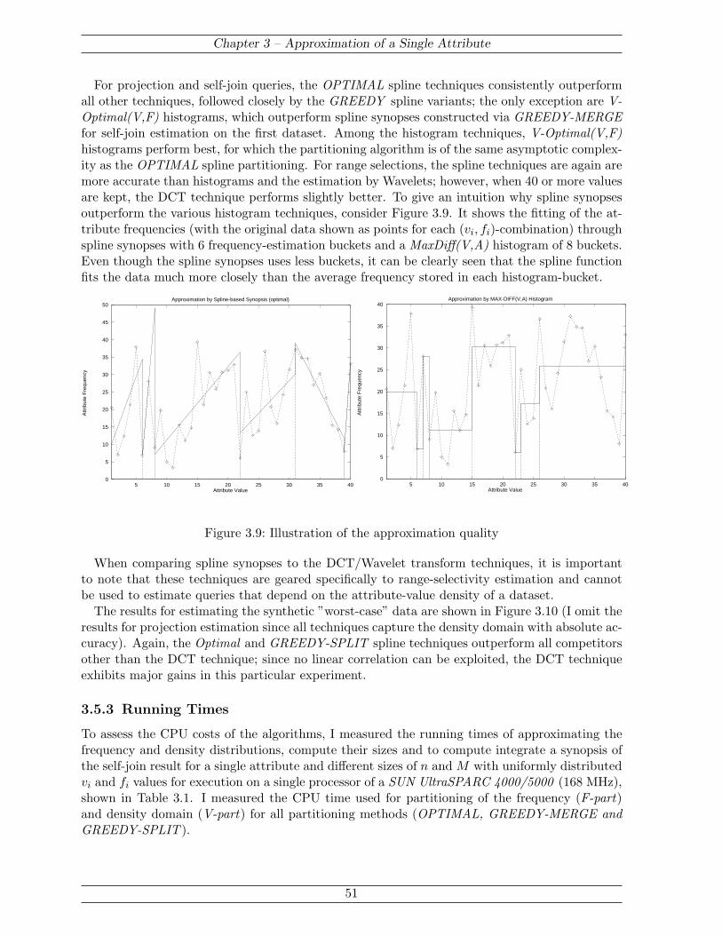
Chapter 3 – Approximation of a Single Attribute
For projection and self-join queries, the OPTIMAL spline techniques consistently outperformall other techniques, followed closely by the GREEDY spline variants; the only exception are V-Optimal(V,F) histograms, which outperform spline synopses constructed via GREEDY-MERGEfor self-join estimation on the first dataset. Among the histogram techniques, V-Optimal(V,F)histograms perform best, for which the partitioning algorithm is of the same asymptotic complex-ity as the OPTIMAL spline partitioning. For range selections, the spline techniques are again aremore accurate than histograms and the estimation by Wavelets; however, when 40 or more valuesare kept, the DCT technique performs slightly better. To give an intuition why spline synopsesoutperform the various histogram techniques, consider Figure 3.9. It shows the fitting of the at-tribute frequencies (with the original data shown as points for each (vi, fi)-combination) throughspline synopses with 6 frequency-estimation buckets and a MaxDiff(V,A) histogram of 8 buckets.Even though the spline synopses uses less buckets, it can be clearly seen that the spline functionfits the data much more closely than the average frequency stored in each histogram-bucket.
0
5
10
15
20
25
30
35
40
45
50
5 10 15 20 25 30 35 40
Attr
ibut
e F
requ
ency
Attribute Value
Approximation by Spline-based Synopsis (optimal)
0
5
10
15
20
25
30
35
40
5 10 15 20 25 30 35 40
Attr
ibut
e F
requ
ency
Attribute Value
Approximation by MAX-DIFF(V,A) Histogram
Figure 3.9: Illustration of the approximation quality
When comparing spline synopses to the DCT/Wavelet transform techniques, it is importantto note that these techniques are geared specifically to range-selectivity estimation and cannotbe used to estimate queries that depend on the attribute-value density of a dataset.
The results for estimating the synthetic ”worst-case” data are shown in Figure 3.10 (I omit theresults for projection estimation since all techniques capture the density domain with absolute ac-curacy). Again, the Optimal and GREEDY-SPLIT spline techniques outperform all competitorsother than the DCT technique; since no linear correlation can be exploited, the DCT techniqueexhibits major gains in this particular experiment.
3.5.3 Running Times
To assess the CPU costs of the algorithms, I measured the running times of approximating thefrequency and density distributions, compute their sizes and to compute integrate a synopsis ofthe self-join result for a single attribute and different sizes of n and M with uniformly distributedvi and fi values for execution on a single processor of a SUN UltraSPARC 4000/5000 (168 MHz),shown in Table 3.1. I measured the CPU time used for partitioning of the frequency (F-part)and density domain (V-part) for all partitioning methods (OPTIMAL, GREEDY-MERGE andGREEDY-SPLIT ).
51
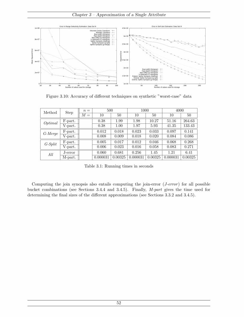
Chapter 3 – Approximation of a Single Attribute
0
2e+07
4e+07
6e+07
8e+07
1e+08
20 30 40 50 60 70 80 90 100
Mea
n S
quar
ed E
rror
Number of values used for storage
Error in Range-Selectivity Estimation: Data Set III
Discrete Cosine TransformWavelet Transform
Equi-width HistogramEqui-depth Histogram
Max-Diff(V,A) HistogramV-Optimal(V,F) HistogramSpline Synopsis (Optimal)
Spline Synopsis (g-split)Spline Synopsis (g-merge)
1e+18
1.5e+18
2e+18
2.5e+18
3e+18
3.5e+18
4e+18
4.5e+18
50 100 150 200 250
Squ
ared
Err
or
Number of values used for storage
Error in Self-Join Estimation: Data Set III
Equi-width HistogramEqui-depth Histogram
Max-Diff(V,A) HistogramV-Optimal(V,F) Histogram
Extend. Spline Synopsis (Optimal)Extend. Spline Synopsis (g-split)
Extend. Spline Synopsis (g-merge)
Figure 3.10: Accuracy of different techniques on synthetic ”worst-case” data
n = 500 1000 4000Method StepM = 10 50 10 50 10 50
F-part. 0.38 1.99 1.98 10.27 51.16 264.63OptimalV-part. 0.38 1.00 1.97 5.93 41.35 133.43F-part. 0.012 0.018 0.023 0.033 0.097 0.141G-MergeV-part. 0.008 0.009 0.018 0.020 0.084 0.086F-part. 0.005 0.017 0.012 0.046 0.068 0.268G-SplitV-part. 0.006 0.023 0.016 0.058 0.083 0.271J-error 0.060 0.681 0.256 1.45 1.21 6.41AllM-part. 0.000031 0.00325 0.000031 0.00325 0.000031 0.00325
Table 3.1: Running times in seconds
Computing the join synopsis also entails computing the join-error (J-error) for all possiblebucket combinations (see Sections 3.4.4 and 3.4.5). Finally, M-part gives the time used fordetermining the final sizes of the different approximations (see Sections 3.3.2 and 3.4.5).
52

4 Approximation of MultidimensionalCorrelation
I could be bounded in a nutshell, and count myselfking of infinite space, were it not that I have baddreams.
– Hamlet
This chapter describes how to extend spline synopses over a single attribute to represent infor-mation on the correlation between multiple attributes. Sections 4.1 and 4.2 give an overview ofthe problems connected with approximating multidimensional data. In Section 4.3 and overviewof my novel approach is given. The approach is based on the use of a space-filling curve originallyproposed by Sierpinski, the properties of which are described in detail in Section 4.4. Section 4.5then describes how the resulting synopses are used for query estimation. Finally, Section 4.6contains an experimental evaluation of the overall approach.
4.1 Multidimensional Partitioning and the “Curse of Dimension-ality”
A straightforward approach to multidimensional approximation would be to extend our tech-nique through the use of multi-dimensional buckets. Then a multi-dimensional attribute valuedistribution could be partitioned into buckets of this type, which would then store a compactrepresentation (of constant size) of the contained values and frequencies.
Unfortunately, such an approach is problematic: because the space of possible partitioningsincreases exponentially with the dimensionality of the data, the problem of finding an optimalpartitioning becomes NP-complete already for much simpler error functions than the ones usedin spline synopsis construction [MPS99]. In addition, to achieve good approximation of the valuedensity in one-dimensional synopses, it was only necessary that the values contained in a bucketwere (approximately) evenly spaced in a single dimension. To achieve good approximation ofvalue density in d dimensions (using constant-size buckets), it becomes necessary for the valuesto be evenly spaced in all d dimensions, which is only the case for high-dimensional distributions.To illustrate the problem, consider the approximation in multidimensional histograms. In eachbucket, the number of distinct values present in each dimension is stored. For purposes of estima-tion it is then assumed that all possible combinations of these values are present, which is knownas the (multi-dimensional) uniform spread assumption. This leads to consistent overestimation ofthe number of attribute values (see Figure 4.1) and underestimation of their frequencies, therebymaking histograms very inaccurate for projection and join estimation in more than a single di-mension. Note that this problem becomes exponentially worse with increase of the dimensionalityof the histogram.

Chapter 4 – Approximation of Multidimensional Correlation
The specification of constant-sized buckets requires the formulation of rigid assumptions onthe placement of attribute values within a single bucket, which typically do not hold for real-lifedata distributions. As a consequence, I use a different approach than the one outlined above.
5HDO�'DWD $SSUR[LPDWLRQ
1A
2A
1A
2A
Figure 4.1: Approximation of multidimensional attribute value distributions in histograms
4.2 Preserving Correlation
As discussed in Section 2.4.1, size estimation for every query specifying filter conditions onmore than one attribute of the same table requires that the estimation technique maintainsthe correlation between attribute values and their frequencies accurately. In addition, it is alsoimportant to maintain the correlation between values of different attributes as well.
To illustrate this, consider a relation R with the attributes Order-Date and Ship-Date(each coded as an integer). These are strongly correlated, in the sense that the value Ship-Dateis typically a fixed number of days larger than Order-Date (or at least has very small variancefor the difference between these dates). Such a data set (250 tuples, requiring 750 values ofstorage) is depicted in Figure 4.2: the values for Order-Date were generated uniformly withinthe interval [1, 500], the values for Ship-Date uniformly within [Order-Date, Order-Date + 10].
Preserving this type of correlation is crucial for a large number of queries, as the conditionsspecifying the inclusion/exclusion of attribute values generally depend on the attribute-valuedistribution. For example a query checking for delayed deliveries:
SELECT DISTINCT ∗ FROM R1 WHERE R1.Ship-Date − R1.Order-Date > 20.
would return no tuples on the original data. Therefore, an estimation technique needs to be ableto preserve the correlation in such a way that none or only very few tuples are returned whenestimating this query.
Figure 4.3 shows the approximation of the data using 30 values of storage space using a 2-dimensional MaxDiff(V,A) histogram (constructed using the MHIST technique). It can be seenthat the use of the uniform spread assumption within buckets limits the ability of histograms (orhistogram-based techniques) to express the present correlation.
As a measure of the amount of correlation present between the attribute values of 2 attributesR.A1, R.A2, I use the Spearman rank-order correlation coefficient [PTVF96], which is defined asfollows. Let Li be the rank of the value of attribute A1 in the i-th tuple, Si be the rank of thevalue of attribute A2 in the i-th tuple (in case of ties, we use the appropriate midrank), and L, S
54

Chapter 4 – Approximation of Multidimensional Correlation
100
200
300
400
500
50 100 150 200 250 300 350 400 450 500
Figure 4.2: Original Data
0
50
100
150
200
250
300
350
400
450
500
0 50 100 150 200 250 300 350 400 450 500
""
Figure 4.3: MHIST Histogram Approximation
the corresponding average rank. Then the linear correlation coefficient of the ranks is defined as
rs =∑|T |
i=1(Li − L)(Si − S)√∑|T |i=1(Li − L)2
√∑|T |i=1(Si − S)2
. (4.1)
The linear correlation coefficient of the example distributions is rs = 0.88, the approximatedistributions resulting from histogram estimation has rs = 0.99, corresponding to the intuitiveinterpretation of Figures 4.2 and 4.3.
Most approximation techniques are geared towards preserving the correlation between attributevalue and the corresponding frequency, but disregard correlation between attribute values.
4.3 Spline Synopses and Mapping Multidimensional Data
First, an injective mapping θ : Rd 7→ R is applied to the attribute-value domain of the base data,reducing the d-dimensional distribution to a one-dimensional one, which is then approximated bythe techniques introduced previously. We store the resulting approximation; when it is used toestimate a multi-dimensional query, the approximated data is mapped back to Rd via the inversemapping ψ := θ−1.
This approach leverages the advantages of the spline techniques discussed previously (efficiency,accurate representation of both attribute frequency and attribute value density, fast computation)while avoiding the rigid requirements of multidimensional buckets (see Section 4.1), the compu-tational overhead entailed by computing the optimal partitioning of multidimensional space andthe lack of accurate value density estimation of transform-based approaches (see Sections 2.4.2and 3.4.3). The only drawback of this approach is an increase in the overhead necessary forestimation of range conditions, because unlike in the one-dimensional case (where buckets cor-respond to intervals containing all values in them) all buckets and values have to be examined,as the bucket boundaries do not have a simple geometrical interpretation. This is discussed indetail in Section 4.5. Figure 4.4 shows the interaction between spline synopses and space-fillingcurves.
4.4 The Sierpinski Space-Filling Curve Construction
Definition 4.1 (Space-Filling Curves) :A Space Filling Curve is a surjective, continuous mapping from the unit interval I1 = [0, 1]to the d-dimensional unit hyper-cube Id = [0, 1]d.
55

Chapter 4 – Approximation of Multidimensional Correlation
Approximation via Spline Synopses
Approximate Data ∈ [0,1)Original Data ∈ [0,1)
Original Data ∈ Rd Approximate Data ∈ Rd
Inverse SFC θ SFC ψ
Figure 4.4: Combining Space-Filling Curves (SFC) and Spline Synopses
The first space-filling curve can be traced to Peano [Pea90]. In 1912 W. Sierpinski proposeda curve construction [Sie12] (Figure 4.7) which is the basis for the curve construction used inthis thesis. While both the Peano and Sierpinski curves described the mapping [0, 1] 7→ [0, 1]d
for d = 2 only, [SR94] extends the construction by Sierpinski to arbitrary values of d. Space-filling curves have successfully been used in a number of applications [Man83], including high-dimensional indexing [KF94, LK01] and graphics compression [DCOM00]; the Sierpinski curvehas also been used for heuristic solutions to the Traveling Salesman Problem with Euclidiandistances [PB89, GS92] and partitioning problems in VLSI design [AK95].
�
�
��
��
�� ��
���
���
���
���
���
������
���
����
����
����
����
����
����
����
����
����
����
����
����
����
����
����
����
Figure 4.5: Successive partitionings of I2 into 2k identical triangles, each containing a k-digitbinary label and a marked vertex for k = 1, . . . , 4
� �
�� ���� ��
������ ��� ������ ��� ������
Figure 4.6: Successive partitionings of the unit interval into 2k identical subintervals, each con-taining a k-digit binary label. The marked endpoint is always on the left. k = 1, . . . , 3
The original Sierpinski curve can be constructed by successively partitioning I2 as shown inFigure 4.5. Here, the k-th partition of I2 consists of 2k identical triangles, each labelled with the
56

Chapter 4 – Approximation of Multidimensional Correlation
binary representation of an integer in the range of 0, . . . 2k − 1. One vertex in each triangle ismarked to distinguish it from the others. The unit interval I1 is similarly partitioned, as shownin Figure 4.6, into subintervals, each labelled and marked at one endpoint.
Each successive partition is obtained by bisecting every triangle or subinterval in the previouspartition. A new label is created by appending an additional digit to the parent’s label; thehalf containing the parent’s marked vertex receives a zero, the other half receives a one. Thespace-filling curve maps each subinterval onto the subtriangle bearing an identical label and itmaps the marked endpoint of the subinterval to the marked vertex of each triangle. The markedvertices are therefore visited in a sequence determined by their labels. The curve resulting fromthis construction is depicted in Figure 4.7. For the first two instances of the curve in the, thevalue corresponding to the position of the vertices in I1 is marked along the curve.
24
34
1516
216
616
04
516
716
1016
816
916
1116
1216
14
416
316
116
016
1416
1316
Figure 4.7: The Sierpinski Curve [Sie12] for d = 2 and k = 2, 4, 6 iterations of the recursiveconstruction
The Sierpinski Curve extension to d dimensions of [SR94] is defined in terms of two iteratedfunction systems (IFS) [Bar88]. The first system W generates a sequence of subdivisions on thehypercube. W defines a family of mappings wi : Rd 7→ Rd as follows:
wi(x1, x2, . . . , xd) =
1/2− (1/2− δ1,i) · x1
1/2− (1/2− δ2,i) · x2...
1/2− (1/2− δd,i) · xd
where δj,i ∈ {0, 1}, j = 1, . . . , d, i = 1, . . . 2d − 1. Each of the 2d members of W is thus uniquelydefined by the vector Di,d = (δ1,i, δ2,i, . . . , δd,i)T . These vectors are now chosen in such a waythat vector Di,d corresponds to the Gray code [Gra53] value for i of length d. The key idea hereis the fact that the Gray codes for two consecutive values of i differ only by one position.
The second system G of 2d iterated functions gi : [0, 1] 7→ subsets of [0, 1] is used to partitionthe unit interval. G is defined as follows:
gi(t) = bd · 2−2d + 2−2d · (i− 1) + 2−d · t, (for 0 ≤ t ≤ 1, i = 1, . . . , 2d − 1) andg0(t) = [t ≤ (2d − bd) · 2−d]− (2d − bd) · 2−2d + 2−d · t (for 0 ≤ t ≤ 1)
with b1 = 1, bk = 2k−1 − bk−1 + 1, k = 2, . . . , d
Let the unit interval [0, 1] be denoted as I1 and the unit hypercube as Id. Now a one-to-onecorrespondence between the system of hypercubes and the sequence of subintervals is defined bymatching the interval defined through t ∈ gi1 ◦ gi2 ◦ . . . gik(I1) with the sub-cube t ∈ wi1 ◦ wi2 ◦. . . wik(Id). As the number of iterations of both iterated function systems approaches infinity,the space-filling curve is obtained (as the limit of this construction). We denote the resultingsurjective mapping as ψ : I1 7→ Id and its inverse as φ := ψ−1 : Id 7→ I1.
57
Chapter 4 – Approximation of Multidimensional Correlation
The overhead for computing the mapping via either φ or ψ of a single point depends on thedimensionality d of the space-filling curve and on the number of iterations t of the IFS. The valuet itself is limited by the accuracy of the data type used to store the values vi and their mapping.To be able to store all possible mapped values after t iterations of the curve construction, theunderlying value type needs to be able to store 2t·(d−1) different values. Consequently, the size oft corresponds to the size (in bits) of this data type divided by d− 1 and is thus a small constant.As a consequence, it becomes necessary for synopses over large number of attributes d, to use adifferent data type for the lowest value in a bucket (for both frequency and density buckets).
Since in any case t is constant, the overhead for computing the mapping of a single value isO(d). When using φ to map values from their original domain to I1 for approximation, themapped values have to be sorted afterwards. Thus, for a data distribution T , the overhead forapproximation increases by O(d·|T |) plus the overhead for sorting |T | values. In my experiments,the overhead for sorting generally dominated the mapping costs.
4.4.1 Properties of the Sierpinski Curve
The Sierpinski curve has a number of salient properties important for its use in connection withspline synopses:
• It contains no distortion, i.e., for arbitrary x, x′ ∈ R, the ranges [x, x + δ], [x′, x′ + δ]correspond to pieces of the curve of identical length.
• It is symmetric (unlike the Hilbert or Peano curve), i.e. invariant to rotations by multiplesof 90 degrees in the direction of each dimensional axis. This means that independent ofwhich dimension the different attributes are mapped to, the approximation quality can beexpected to be similar.
• The mapping ψ preserves the Lebesque measure in the following sense: for every Borel setA ⊆ Id
µ1(φ(A)) = µd(A) [SR94],
when µ1 and µd are the Lebesque measure in R and in Rd respectively. Intuitively, this canbe interpreted as the fact that the Sierpinski curve fills Id with uniform density everywhere.
• The resulting projection ψ preserves distances very well, as ψ is a Lipschitz continuousmapping of order 1/d, in the following sense:
∀v1, v2 ∈ [0, 1] : ‖ψ(v1)− ψ(v2)‖ ≤ 2√
d + 6 |v1 − v2|1d [SR94] (4.2)
with ‖ · ‖ denoting the L2 norm (Euclidian Distance) between the data points in Rd. Thisis optimal in the sense that it can be shown that a surjection from I1 to Id that is Lipschitzcontinuous of order σ > 1/d is not possible [Mil80].
The last property is crucial for the use of the Sierpinski curve for the estimation of (multi-dimensional) attribute value density. Consider the case of a d-dimensional value distributionV = {v1, . . . , vn}. Each value vi ∈ Rd is then mapped to a value vlin
i ∈ [0, 1], by normalizing eachvalue (i.e., dividing the i-th component of vi by the highest value in the corresponding domain, fori = 1, . . . , d) and then applying φ. I then approximate the mapped values V lin := {vlin
1 , . . . , vlinn }
as V lin := {vlin1 , . . . vlin
n }, minimizing∑|T |
i=1(vlini − vlin
i )2. In order to use the resulting approxi-mation for query estimation, the vlin
i are mapped back via ψ at query processing time and thenormalization reversed (i.e., the i-th component of ψ(vlin
i ) is multiplied by highest value in the
58

Chapter 4 – Approximation of Multidimensional Correlation
corresponding domain, for i = 1, . . . , d). Because of Equation 4.2, the final approximation errorfor a value vi (i.e., ‖ψ(vlin
i )− ψ(vlini )‖) is limited by the upper bound of 2
√d + 6 |vlin
i − vlini |
1d .
Therefore, the process of constructing a synopsis over d-dimensional minimizes an upper boundfor the overall approximation error
|T |∑
i=0
(fi − fi)2 + v domainf domain · (‖vi − vi‖)2. (4.3)
Unlike in the case of one-dimensional synopses, where the overall approximation error is min-imized, the synopsis construction is only optimal with regard to the (mean squared) error inI1, but not with regard to the error in Rd. However the notion of minimizing the upper boundfor Equation 4.3 and minimizing the equation itself coincide for all practical purposes when thelarge data distribution to be estimated becomes large, as the different mappings of a distancein I1 to different distances in Id distances average out. In this sense (and the interests of asimple notation), I refer to the spline synopsis construction in higher dimensions as minimizingEquation 4.3.
Because our approach means that no rigid assumptions on the placement of attribute valueswithin a bucket are used, the resulting estimation preserves correlation between values of differentattributes much better. Consider the example data shown in Figure 4.2. The approximation ofthis data using a spline synopses requiring 30 values storage is shown in Figure 4.8. Not onlydoes this estimation resemble the shape of the original data much more than the histogramapproximation (Figure 4.3), it also has a linear correlation coefficient rs = 0.83 much closer tothe original one.
50
100
150
200
250
300
350
400
450
50 100 150 200 250 300 350 400 450
""
Figure 4.8: Spline Synopsis Approximation
4.5 Using Multidimensional Spline Synopses for Query Estima-tion
The key difference between multidimensional and one-dimensional spline synopses is that the geo-metrical interpretation (in Id) of a bucket’s boundaries are fractals themselves (not d-dimensionalranges as with multidimensional histograms). Therefore, information on the bucket bound-aries cannot be leveraged efficiently to eliminate buckets from consideration for range-selectionqueries1. Instead, all attribute values have to be materialized and mapped back using ψ beforefiltering, resulting in O(d · |T |) overhead, as discussed in Section 4.4. Still, as d is generally a
1However, the process of transforming a d-dimensional range query into a set of one-dimensional range-queries,that may then be evaluated using all optimizations introduced in Section 3.4 is straightforward. Initially,all intersections between the curve and the range-boundaries are computed. As the curve itself is a fractal,
59
Chapter 4 – Approximation of Multidimensional Correlation
small value (with the possible exception of materialized views in large decision-support systems,relations used in databases generally have less than 15 attributes), this approach is still suffi-ciently fast to be used in query optimization. Otherwise, the overall approach remains the sameas for one-dimensional synopses (Section 3.4).
4.6 Experiments
The Techniques: I compare spline synopses with two multidimensional MaxDiff(V,A) his-tograms computed using the MHIST-2 partitioning algorithm, which were found to be the mostaccurate histogram technique for multidimensional data [PI97]. In addition, for workloads con-sisting solely of range selections, I also examine the accuracy of discrete transform techniquesbased either on the Wavelet transform [MVW98], using Haar Wavelets, or the discrete cosinetransform (DCT) [LKC99].
Datasets: The experiments on multidimensional distributions were carried out on two data sets:(1) 1970 PUMS Census data, of which we use the attributes migplac5 and chborn (661 uniqueattribute-value pairs, 70817 tuples), provided by the KDD Archive [KDD], and (2) a syntheticstress test similar to the one used before, with 400 unique value pairs, 10000 tuples, and randomlychosen density distribution and attribute-value frequencies.
Query Workload: First, an approximation of each data set is computed, which is then usedfor three different estimation tasks:
(a) Estimating the size |V| range-selection queries of the type SELECT * FROM R1 WHERER1.A1 < v1 AND R1.A2 < v2, which are issued for all values (v1, v2) ∈ V. The accuracyfor this type of estimation depends on both the attribute value frequency approximationand the attribute value density approximation.
(b) Estimating the size |V| projection queries of the type SELECT DISTINCT * FROM R1 WHERER1.A1 < v1 AND R1.A2 < v2, which are issued for all values (v1, v2) ∈ V. The accuracyof this type of estimation depends on attribute value density approximation.
In each case I measure the mean squared error
MSE :=1n
∑
i=1,...,n
(exact sizei − approx sizei)2,
with n being the number of queries.
4.6.1 Results
The results of the two experiments on multi-dimensional data are shown in Figures 4.9 and 4.10.For range-selectivity estimation the histogram-based techniques consistently outperformed themultidimensional MaxDiff(V,A) histograms. Wavelets turned out to be superior to splines for
the number of such intersections is infinite in theory, however, because of the limited accuracy of the datatypes used to store the mapped values, the curve is only computed for a limited number t of iterations of thecurve construction (see Section 4.4), resulting in a limited number of intersections (for a detailed treatmentof this topic with regards to the Hilbert curve, see [MJFS01]). Now the intervals along the curve connectingtwo of these intersections (without another intersection in between) encompass values that satisfy the rangecondition. Furthermore, each of these ranges corresponds to a one-dimensional range in I1. Thus, the result ofthe d-dimensional range query can be estimated as the union of the results for all these one-dimensional rangequeries.
60
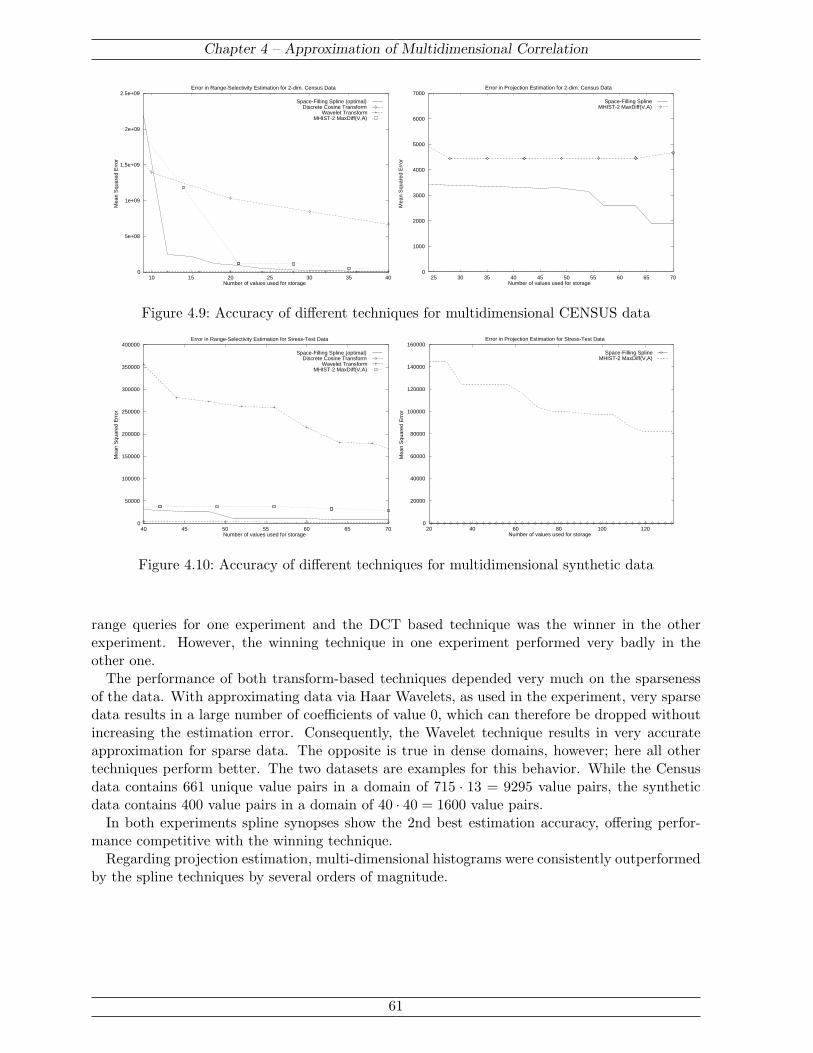
Chapter 4 – Approximation of Multidimensional Correlation
0
5e+08
1e+09
1.5e+09
2e+09
2.5e+09
10 15 20 25 30 35 40
Mea
n S
quar
ed E
rror
Number of values used for storage
Error in Range-Selectivity Estimation for 2-dim. Census Data
Space-Filling Spline (optimal)Discrete Cosine Transform
Wavelet TransformMHIST-2 MaxDiff(V,A)
0
1000
2000
3000
4000
5000
6000
7000
25 30 35 40 45 50 55 60 65 70
Mea
n S
quar
ed E
rror
Number of values used for storage
Error in Projection Estimation for 2-dim. Census Data
Space-Filling SplineMHIST-2 MaxDiff(V,A)
Figure 4.9: Accuracy of different techniques for multidimensional CENSUS data
0
50000
100000
150000
200000
250000
300000
350000
400000
40 45 50 55 60 65 70
Mea
n S
quar
ed E
rror
Number of values used for storage
Error in Range-Selectivity Estimation for Stress-Test Data
Space-Filling Spline (optimal)Discrete Cosine Transform
Wavelet TransformMHIST-2 MaxDiff(V,A)
0
20000
40000
60000
80000
100000
120000
140000
160000
20 40 60 80 100 120
Mea
n S
quar
ed E
rror
Number of values used for storage
Error in Projection Estimation for Stress-Test Data
Space-Filling SplineMHIST-2 MaxDiff(V,A)
Figure 4.10: Accuracy of different techniques for multidimensional synthetic data
range queries for one experiment and the DCT based technique was the winner in the otherexperiment. However, the winning technique in one experiment performed very badly in theother one.
The performance of both transform-based techniques depended very much on the sparsenessof the data. With approximating data via Haar Wavelets, as used in the experiment, very sparsedata results in a large number of coefficients of value 0, which can therefore be dropped withoutincreasing the estimation error. Consequently, the Wavelet technique results in very accurateapproximation for sparse data. The opposite is true in dense domains, however; here all othertechniques perform better. The two datasets are examples for this behavior. While the Censusdata contains 661 unique value pairs in a domain of 715 · 13 = 9295 value pairs, the syntheticdata contains 400 value pairs in a domain of 40 · 40 = 1600 value pairs.
In both experiments spline synopses show the 2nd best estimation accuracy, offering perfor-mance competitive with the winning technique.
Regarding projection estimation, multi-dimensional histograms were consistently outperformedby the spline techniques by several orders of magnitude.
61
5 Physical Design for Data Synopses
According to an optimist, the glass is half-full,according to a pessimist, the glass is half-empty,according to an engineer, the glass has twice the necessarysize.
– Unknown
5.1 Introduction
In this chapter, I develop a novel framework for and algorithmic solution to the physical designproblem for data synopses, covering the entire class of SPJ (i.e., select-project-join) queries. Incontrast to the work in [CN00], the approach goes beyond the binary decisions on building vs.not building a certain synopsis by addressing the fundamentally important issue of how muchmemory each synopsis should be given. This is especially important when the role of statisticsmanagement goes beyond choosing good query execution plans, and synopses also serve to predictabsolute run-times and result sizes, which in turn is highly relevant in data mining or Web sourcemediation environments. I characterize the exact solution for the optimal choice of synopses fora given workload. For complexity reasons, I derive various problem-specific heuristics that makemy approach reasonably efficient and thus practical.
The chapter is organized as follows. First, it is necessary to introduce additional notation inSection 5.2. In Section 5.3 the underlying optimization problem and the used error model aredefined. Section 5.4 then describes how to determine the optimal set of synopses exactly, usingtwo assumptions which (in earlier experiments) have been found to hold for nearly all datasetsand which lead to a compact formulation of the necessary computations. For large instancesof the optimization problem, I discuss several heuristics to remove potential bottlenecks. InSection 5.7 it is then shown how to combine the various building blocks of the framework into aunified algorithm. Section 5.8 contains an empirical validation of the approach in form of severalexperiments conducted with the TPC-H decision support benchmark.
5.2 Notation
I consider a set of queries Q := {Q1, . . . , Q|Q|}. Queries can be “approximately answered” by aset of synopses S := {S1, . . . , Sl} corresponding to the data distributions T1, . . . , Tl. Because inour context there is never more than one synopsis for a given set of attributes I also write SA withA being the set of attributes captured by the synopsis, i.e., S{R1.A2,R1.A3} denotes the synopsisover the two attributes A2 and A3 of relation R1. Analogously, we use the notation T{R1.A2,R1.A3}to describe the corresponding joint data distribution in the full data set. The size of a synopsisSA (in terms of the number of values necessary to store SA) is denoted by Size(SA).
A simple (range) selection or projection query can be answered using the data distributionof the queried relation over the attributes involved in the range selection. A join query can be

Chapter 5 – Physical Design for Data Synopses
processed by examining the joint data distribution of the joining relations. Thus it is possible toassign to each query Qi on relation Rp the minimum set of attributes Min(Qi) ⊆
⋃Rp∈RAtt(Rp),
whose joint data distribution must be examined to answer the query. For example consider thequery q1
SELECT R1.A1 WHERE R1.A2 > 100.
This query can be answered by examining the joint data distribution of relation R1 over theattributes R1.A1 and R1.A2, thus Min(q1) = {R1.A1, R1.A2}.
When only the size of a result is of interest (for example in the context of query optimization),it is sufficient to query the attributes that determine the number of tuples in the result; assumingthat no duplicate elimination is performed, in this case the minimum set becomes Min(q1) ={R1.A2}. Consequently, the set Min(Qi) contains the information which synopses need to bebuilt in order to answer query Qi while observing all correlations between the relevant attributes.
As join synopses have been shown to be vital to accurate estimation of joins for nearly allreal-life datasets (see Sections 3.4.3 and 3.4.6), I adopt the following approach for all queriesin Q involving joins. For each query Qi involving one or more joins, I add a “virtual relation”R′ to R representing the joint data distribution of the top node in the corresponding join tree(i.e. the complete n-way join if the join tree has n leaves). A query involving a join could thusbe modelled by introducing join synopsis over the relevant attributes from the joining relations;consider query q2:
SELECT R1.A1 FROM R1, R2, R3 WHERE R1.A2 = R2.A3 AND R2.A4 = R3.A5
Here I introduce R′ := R1A2=A3
./ R2A4=A5
./ R3. Then Min(q2) = {R′.A1}. Note that it isonly necessary to introduce this R′ if is not present already. If q2 appears more than once inthe workload (either solitary or as a sub-query), R′ is still only introduced once. This approachcorresponds to introducing a full join synopsis (see Section 3.4.4) for every unique join presentin the workload.
5.3 Framework
The physical design problem for data synopses is defined as follows:
Definition 5.1 (Physical Design Problem for Data Synopses) :When given a number of datasets R := {R1, . . . , Rn}, a workload consisting of SPJ (select-project-join) queries Q := {Q1, . . . , Qk} and a limited amount of available memory M ,the physical design problem for data synopses is to determine the best combination S ofsynopses that can be stored using up to M memory, so that the estimation error over allqueries is minimized.
This corresponds to the natural goal of maximizing accuracy for query optimization, approximatequery answering, or minimizing the query time when supporting top-k queries [CG99]. If thesynopses in S are only used for query optimization, additional pruning of S may be beneficial, assynopses that do not influence plan selection can be omitted (see [CN00]); in addition, maximizingthe estimation accuracy for the final set of selected synopses (in this case, by tuning their sizes)can further improve query optimization.
In the following, it is assumed that each query Qi is mapped to exactly one synopsis Sj ∈ Swhich captures all attributes that are relevant for Qi, i.e., attributes on which filter conditions are
63
Chapter 5 – Physical Design for Data Synopses
defined as well as attributes that appear in the SELECT clause of the query (see Section 2.2). Thisis no limitation, as it is always possible to decompose a more complex query into subqueries suchthat the above condition holds for each subquery, when full join synopses are used for each joinin the workload. In fact, an SPJ query would often be the result of decomposing a complex SQLquery (e.g., to produce an intermediate result for a group-by and aggregation decision-supportquery). The subqueries that matter in this context are those for which I wish to estimate theresult or result size. In commercial query engines and in most of the prior work on data synopses,these subqueries were limited to simple range selections. This approach improves the state of theart in that we consider entire SPJ queries as the building blocks for data synopses.
5.3.1 Storage of Multiple Synopses
In the discussed scenario, the database system has to store multiple synopses over a number ofdifferent attribute combinations. Therefore, in addition to the buckets stored by each synopsisitself, the following bookkeeping information needs to be stored to construct a directory of allsynopses:
(1) the relation approximated by the synopsis,(2) the combination of attributes approximated by the synopsis (coded as a bit vector),(3) the total number of buckets,(4) the number of buckets used for frequency approximation,(5) the highest attribute value stored in the synopsis/relation, and(6) a pointer to the synopsis itself.
Consequently, each synopsis requires additional 6 values storage for this bookkeeping information.As discussed in Section 4.4, the values used for (2) and (5) may be represented by a different (i.e.,larger) data type than the other values, when the number of attributes stored in the correspondingsynopsis is very large. This will later be important in connection for the proof of Theorem 5.
5.3.2 The Error Model
The overall goal is to minimize the estimation error over all queries Qj ∈ Q. First considera scenario in which all queries only depend on a single synopsis S0 over the data distributionT = {(v1, f1), (v2, f2), . . . , (vn, fn)}. I define the error for a given query Qj ∈ Q by characterizinghow well the query result Result(Qj) ⊆ T is approximated. Then I define the error over allqueries in Q with respect to a data distribution T as
Error(Q, S0) :=∑
Qj∈Q
( ∑
i∈{k|vk∈Result(Qj)}(fi − fi)2 + r · (‖vi − vi‖)2
)(5.1)
with the factor r determining the importance of frequency-approximation relative to the im-portance of density approximation. Thus, if the weights wi are defined as wi := |{Q′ | vi ∈Result(Q′), Q′ ∈ Q}|, and the factor1 v domain/f domain is used for r, the sum of the errorsfor each query posed to synopsis S0 can be written as:
Error(Q, S0) :=|T |∑
i=1
wi · (fi − fi)2 + v domainf domain · wi · (‖vi − vi‖)2, (5.2)
1The choice of the value r does not influence the algorithmic properties of the approach, as any value for r caneasily be incorporated into the reconciliation of frequency and density synopses described in Section 3.3.2.
64
Chapter 5 – Physical Design for Data Synopses
with the appropriate values for f domain and d domain. Except for the weights wi, this isthe error function (Equation 4.3) minimized (in the sense described in Section 4.4) by splinesynopses. Since the weights wi can be easily incorporated into the spline construction process(see Section 3.3.5), minimizing the query error in the case of a single distribution has become aproblem of constructing the optimal spline synopsis.
This is a slight simplification as it ignores approximation errors with regard to the boundaryconditions of a query: when using a synopsis for answering a query some attribute values vi
may be included in the approximate answer even though the corresponding vi would not bein the query result. Likewise, some attribute values may be erroneously excluded. However,incorporating these effects into our model would result in an optimization problem of intractablecomplexity.
In a scenario with multiple synopses S := {S1, . . . , Sl}, each query Qj is answered (dependingon Min(Qj)) by a synopsis in S. To assign each queried attribute combination to exactly onesynopsis, a mapping function
map :⋃
2{Att(R)|R∈R} 7→ {1, . . . , l} (5.3)
is used. I will describe how to automatically obtain this mapping in Section 5.4.2.Note that this model assumes that queries over the same attribute combination are always
mapped to the same synopsis (otherwise it would be necessary to store additional informationon the mapping of specific queries, which would in turn compete for the memory available forsynopses). Thus, the error over a set of synopses S := {S1, . . . , Sl} is defined as:
Error(Q,S) =l∑
i=1
(Error({Qj ∈ Q | map(Min(Qj)) = i}, Si).
Since the error of each synopsis Si is dependent on the memory size Size(Si) of the synopsis,this is more accurately stated as:
Error(Q,S) = min(Size(S1),...,Size(Sl))∈Nl
l∑
i=1
(Error({Qj ∈ Q | map(Min(Qj)) = i}, Si)) (5.4)
under the constraint that∑l
i=1 Size(Sl) is equal to the memory size M available for all synopsestogether. Thus the problem of optimizing the estimation error for the entirety of queries in theworkload can be seen as a problem of selecting the optimal set of synopses and choosing theirsizes.
5.4 Synopsis Selection and Memory Allocation
To illustrate the issues involved in the selection of the optimal set of synopses, consider a workloadQ = Q1 ∪ Q2, Q1 containing no1 queries Q′ (i.e., queries of type Q′ whose fraction in the entireworkload is proportional to no1) with Min(Q′) = {{R1.A1}} and Q2 containing no2 queries Q′′
with Min(Q′′) = {{R1.A2}}. Then these can be answered by either
(a) two synopses S{R1.A1} and S{R1.A2} over each single attribute(b) one synopsis S{R1.A1,R1.A2} over the joint data distribution of R1.A1 and R1.A2.
65

Chapter 5 – Physical Design for Data Synopses
Therefore, to compute the optimal error for the overall available memory M we have to evaluate
Error(Q) :=
min{Error for combination (b)︷ ︸︸ ︷
Error(Q, S{R1.A1,R1.A2}) , (with Size(S{R1.A1,R1.A2}) = M)
minSize(S{R1.A1})∈NSize(S{R1.A2})∈N
(Error(Q1, S{R1.A1}) + Error(Q2, S{R1.A2})
)
︸ ︷︷ ︸Error for combination (a)
}(with Size(S{R1.A1}) + Size(S{R1.A2}) = M)
and keep track of the resulting synopses and memory partitioning. So the problem of computingthe optimal set of synopses (and the corresponding memory allocation) becomes a two-stepprocess:
(1) Computing Error(Q′, Sx) for all candidate synopses Sx and all possible combinations ofqueries Q′ ⊆ Q that may be mapped to Sx and the maximum amount of Memory Mto be used for Sx. This requires O(M · |Tx|2) steps (for the OPTIMAL partitioning, seeSection 3.1.3) for each pair of Sx and Q′ and also generates the values of Error(Q′, Sx) forall values of Size(Sx) ≤ M .
(2) Selecting the optimal set of synopses from a set of candidates computing an optimal memorypartitioning such that the weighted sum over all synopsis errors (weighted by the numberof times each synopsis is queried) becomes minimal for the synopses included in the optimalsolution. Since the weights change according to the combinations of synopses in the solu-tion, this is a different and more difficult problem than finding the optimal combination ofsynopses for different relations. It will be shown in Section 5.4.2, the problem of synopsisselection and memory partitioning are closely related and thus solved together.
In the following (Sections 5.4.1 and 5.4.2), I will show how to solve the above problem for asingle dataset R ∈ R. The sub-solutions for all datasets in R can then be combined to solve theoverall problem (Section 5.4.3). Since the resulting solutions are computationally expensive, Iwill describe in Section 5.6 how to reduce the computational cost through the use of heuristics.
The key idea of my approach is to use two properties that hold for over the plethora of query(size) estimation techniques to prune the search space of all possible combinations of synopsesand their sizes significantly. While both properties were found to hold for all combinations ofqueries and data sets tested in this thesis, only one of them can be shown to hold for everyquery/data combination possible. For the other property datasets can be constructed, for whichit does not hold; therefore it should be seen as an efficient heuristic.
5.4.1 Pruning the Search Space
Note that in the example of Section 5.4 the combinations S ′ = {S{R1.A1}, S{R1.A1,R1.A2}} orS ′′ = {S{R1.A2}, S{R1.A1,R1.A2}} were never considered. This is due to a simple property of splinesynopses, which also generally holds for both histograms and Wavelet-based approximations:
Observation 5.1 “Pruning Property” :When answering queries over the set of attributes a, a synopsis Sx, over the set of attributesx with a ⊆ x will yield more accurate answers than a synopsis Sy if x ⊂ y and both synopsesare of identical size.
66

Chapter 5 – Physical Design for Data Synopses
While artificial data distributions can be constructed that do not obey the above observation,the pruning property was found to hold in all experiments on real-life datasets. The intuitionbehind it is the fact that by including more attributes in a synopsis, the number of uniqueattribute-value combinations vi in the corresponding data distribution increases as well (in thisrespect, the synopsis selection problem is similar to the one of index selection), making it harderto capture all attribute values/frequencies with acceptable accuracy.
In the above case, it means that S{R1.A1} answers queries posed to R1.A1 better thanS{R1.A1,R1.A2} (using the same memory). Similarly S{R1.A2} is an improvement over S{R1.A1,R1.A2}for queries posed to R1.A2. Thus the combination S = {S{R1.A1}, S{R1.A2}} generally outperformsS ′ or S ′′.
Using the above observation, it becomes possible to characterize the set of candidate synopsesin a compact manner. Consider a single relation R. Then the sets of attribute combinations ofR queried is
Syn(R,Q) := {Min(Qi) | Qi ∈ Q}Now the set of all candidate synopses for R can be defined as:
Cand(R,Q) := {Sx | x =⋃
z, z ⊆ Syn(R,Q)}
This means that the set of all candidate synopses forms a lattice (see Figure 5.1) over theattribute-combinations queried; e.g. if the set of all queried attribute combinations is
Syn(R,Q) = {{R.A1}, {R.A2}, {R.A2, R.A3}, {R.A3}}
then the set of candidate synopses becomes
Cand(R,Q) ={{R.A1}, {R.A2}, {R.A3}, {R.A1, R.A2}, {R.A1, R.A3}, {R.A2, R.A3}, {R.A1, R.A2, R.A3}}.
The intuition behind the definition of Cand(R,Q) is the following: if a Synopsis Sy is in
2A1A
321 AAA
21AA 32AA
3A
31AA
Figure 5.1: The lattice of candidate synopses
Cand(R,Q), it must be considered, for it is the most efficient way to answer a subset of queriesof R using only one synopsis (all other synopses capable of answering the same subset would beless efficient, due to the pruning property). Conversely, if Sy 6∈ Cand(R,Q) then y must be ofthe form y = cand ∪ nocand with cand ∈ {⋃ z, z ⊆ Syn(R,Q)}, nocand ⊆ Att(R), and ∀x ∈nocand : (cand ∪ x) 6∈ {⋃ z, z ⊆ Syn(R,Q)}. But then Scand answers the same set of queries asSy and does so more efficiently, since cand ⊂ y.
In addition to the pruning property, I utilize a second property of spline synopses to prune thesearch space even further.
67

Chapter 5 – Physical Design for Data Synopses
Observation 5.2 “Merge Property” :For a set of queries Q each querying the same combination of attributes A, the error foranswering the queries using one synopsis S over A with M memory is smaller than theerror using two synopses S1, S2 over A, which together use memory M .
The intuition for this property is the following: By joining the synopses S1 and S2, the esti-mation for the (potentially) overlapping regions in S1 and S2 is improved, as additional memoryis invested in its estimation. It is a trivial consequence that the merge property also holds forcombinations of more than two synopses over A. In contrast to the pruning property, it is possibleto prove that the merge property always holds.
Theorem 5. For a set of queries Q over the same attribute combination A, the error for an-swering these queries by a single synopsis Sunion is less to or equal to the error for Q with twosynopses S1, S2, which together require the same amount of memory as Sunion.
Proof: In Section 5.3.2 it was shown that the error for a set of queries corresponds to the error ofthe fitting-problem posed in Equation 5.2. Therefore, if I can show that the value for Equation 5.2is smaller for Sunion than for S1 and S2, the overall statement follows.
This will be done in the following manner: Based on a given S1, S2 and Q, I will constructa corresponding Sunion in terms of the bucket-partitioning used for fitting attribute frequenciesand values. I will show that the overall error is less or equal for Sunion; now, since our parti-tioning method for constructing spline synopses traverses the space of all possible partitionings,either Sunion or a synopsis with better overall error will result from running the spline synopsesconstruction on Q.
First, it is necessary to consider the storage requirements for spline synopses: buckets for bothfrequency- and attribute-value approximation store 3 values (see Section 3.3.1); in addition, a to-tal of 6 values storage for bookkeeping information is required (see Section 5.3.1). Therefore, eachsynopsis requires 6 + 3 · (number of buckets) of storage. Because no further further bookkeepinginformation is stored, it is necessary to require that each synopsis approximates all values be-tween the lowest and highest value stored2. Otherwise it would not be possible to decide whetherat run-time whether a query can be approximated by a synopsis or not, for the incoming queriesmay not be part of the workload the synopses were constructed over.
I also need to introduce the following notation: Define F Erri as the respective error forthe problem of fitting the frequencies (i.e.
∑Ti=0 wi · (fi − fi)2) in Synopsis Si. Define the
constraint error F Erri[low,high) as
∑high−1i=low wi ·(fi−fi)2 for Si. Define D Erri and D Erri
[low,high)analogously, only with regard to fitting of the attribute-values.
Define Ii = [vstarti , vendi) as this interval of the values approximated by Si. If I1 and I2 overlap,it has to be decided to which synopses to map the (parts of) queries in Q querying I1∩I2. As it isnot possible to map every single query to a synopsis individually without introducing additionalinformation, each query (part) querying the interval I1 ∩ I2 is mapped to the synopsis with thelower overall error in the area of intersection.
Without loss of generality I assume that vstart1 ≤ vstart2 . For purposes of approximation,each interval Ij is partitioned into buckets; I define a partitioning into k buckets as a k − tuple
P = (lowj1, . . . , low
jk) corresponding to the buckets [v
lowj1, v
lowj2), . . . , [v
lowjk, vendj ).
Now, given synopses S1 using b1 buckets (of which bf1 are used for frequency-approximation)
and S2, using b2 buckets (bf2 defined analogously), I construct Sunion with at most b1 + b2 + 2
2For synopses over more than one attribute, it suffices to require that all values between the highest and lowestvalue in I1 after the mapping by the space-filling curve are stored.
68
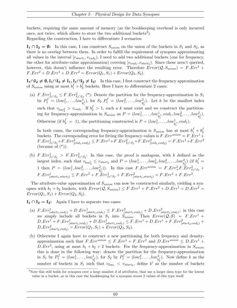
Chapter 5 – Physical Design for Data Synopses
buckets, requiring the same amount of memory (as the bookkeeping overhead is only incurredonce, not twice, which allows to store the two additional buckets3).Regarding the construction, I have to differentiate 3 scenarios:
I1 ∩ I2 = ∅: In this case, I can construct Sunion on the union of the buckets in S1 and S2, asthere is no overlap between them. In order to fulfill the requirement of synopses approximatingall values in the interval [vstart1 , vend2), I need to add two additional buckets (one for frequency,the other for attribute-value approximation) covering [vend1 , vstart2). Since these aren’t queried,however, this doesn’t influence the resulting error. Therefore Error(Q, Sunion) = F Err1 +F Err2 + D Err1 + D Err2 = Error(Q1, S1) + Error(Q2, S2).
I1∩I2 6= ∅, I1∩I2 6= I1, I1∩I2 6= I2: In this case, I first construct the frequency approximationof Sunion using at most bf
1 + bf2 buckets. Here I have to differentiate 2 cases:
(a) F Err1I1∩I2
≤ F Err2I1∩I2
(*): Denote the partition for the frequency-approximation in S1
by P f1 = (low1
1, . . . , low1bf1
), for S2 P f1 = (low2
1, . . . , low2bf2
). Let k be the smallest index
such that vlow2k
> vend1 . If bf2 > 1, such a k must exist and we construct the partition-
ing for frequency-approximation in Sunion as P = (low11, . . . , low
1bf1
, end1, low2k, . . . , low
2bf2
).
Otherwise (if bf2 = 1), the partitioning constructed is P = (low1
1, . . . , low1bf1
, end1).
In both cases, the corresponding frequency-approximation is Sunion has at most bf1 + bf
2
buckets. The corresponding error for fitting the frequency-values is F Errunion = F Err1+F Err1
I1∩I2+F Err2
[end1,end2) ≤ F Err1+F Err2I1∩I2
+F Err2[end1,end2) = F Err1+F Err2
(because of (*)).
(b) F Err1I1∩I2
> F Err2I1∩I2
: In this case, the proof is analogous, with k defined as thelargest index, such that vlow1
k≤ vstart2 and P = (low1
1, . . . , low1k, low
21, . . . , low
2bf2
) (if bf1 =
1 then P = (low11, low
21, . . . , low
2bf2
)). In this case F Errunion = F Err2+F Err2
I1∩I2+
F Err1[start1,start2) ≤ F Err2 + F Err1
I1∩I2+ F Err2
[start1,start2) = F Err1 + F Err2.
The attribute-value approximation of Sunion can now be constructed similarly, yielding a syn-opses with b1 + b2 buckets, with Error(Q, Sunion) ≤ F Err1 + F Err2 + D Err1 + D Err2 =Error(Q1, S1) + Error(Q2, S2).
I1 ∩ I2 = I2: Again I have to separate two cases:
(a) F Err1[start1,end1) + D Err1
[start1,end1) ≤ F Err2[start1,end1) + D Err2
[start1,end1): in this casewe simply include all buckets in S1 into Sunion. Then Error(Q,S) = F Err1 +D Err1 + F Err1
[start1,end1) + D Err1[start1,end1) ≤ F Err1 + D Err1 + F Err2
[start2,end2) +D Err2
[start2,end2) = Error(Q1, S1) + Error(Q2, S2).
(b) Otherwise I again have to construct a new partitioning for both frequency and density-approximation such that F Errunion ≤ F Err1 + F Err2 and D Errunion ≤ D Err1 +D Err2, using at most b1 + b2 + 2 buckets. For the frequency-approximation in Sunion
this is done in the following way: denote the partition for the frequency-approximationin S1 by P f
1 = (low11, . . . , low
1bf1
), for S2 by P f1 = (low2
1, . . . , low2bf2
). Now define k as the
number of buckets in S1 such that vlowi < vstart2 , define k′ as the number of buckets3Note this still holds for synopses over a large number d of attributes, that use a larger data type for the lowest
value in a bucket, as in this case the bookkeeping for a synopsis stores 2 values of this type itself.
69

Chapter 5 – Physical Design for Data Synopses
in S1 such that vlowi ≥ vend2 . Then I construct P = (low11, . . . , low
1k, low
21, . . . , low
2bf2
,
end2, low1k′ , . . . , low
1bf1
). This results in k+1+bf2 +(bf
1−k′+1) buckets, which is at most bf1 +
bf2+1, since k′−k ≥ 1. The resulting error for approximation of value frequencies is F union =
F Err1[start1,start2) + F Err2. The construction for the attribute-value approximation is
similar.
Because both of these properties typically apply also to approximation by histograms orwavelets, the following results also apply to the physical design problem when these techniquesare used as base synopses4. It is necessary to use a different error measure, however, as it is notpossible to match pairs of values and frequencies in the original data and the approximation,because the size of a data distribution |Tx| is not invariant when approximated by either of thesetechniques. Instead, I suggest the use of an error measure that tracks the difference betweenthe actual and the approximated data distribution, and computes its own matching, such as theMAC distance [IP99] or the error-metric introduced for join-errors in Section 3.4.4.
5.4.2 Selecting the Synopses for a Single Relation R
In the following I will describe, for a given set Q of queries over a single relation R, how tocompute the optimal combination S of synopses, their sizes, and the corresponding mapping ofqueries, such that all queries can be answered and the overall error becomes minimal.
The problem resembles the issue of selecting the optimal set of (multicolumn) indices for a givenworkload, as the trade-off is similar: by selecting a synopsis or an index over a larger number ofattributes, the number of queries this synopsis or index supports is increased, while at the sametime its cost also rises. However, the synopsis selection problem is unique, and substantially moredifficult, for a number of reasons:
(1) The size of the synopsis for a given attribute combination is not fixed. Therefore, a synopsisthat provides poor estimations at size m might be quite useful at size m′,m′ > m. Sonot only all potential combinations of synopses have to evaluated, but also all possiblecombinations of their sizes.
(2) A standard B-tree index over attributes A1, . . . , Ah can be used to support queries over anyprefix A1, . . . , Ah′ , h
′ ≤ h; thus the presence of such an index makes indexes over prefixessuperfluous. In contrast, a synopsis over the set of attributes A = {A1, . . . , Ah} can answerqueries over all subsets of A, but because the approximation quality deteriorates with theinclusion of additional attributes (see Section 5.4.1), additional synopses over subsets of Amay still be beneficial.
(3) The maintenance costs of data synopses are only a second-order issue, as synopses donot have to be constantly kept up-to-date, but can be re-computed once their accuracydeteriorates too far.
Therefore, exact or heuristic optimization methods for index selection, such as the formulation asa 0-1 integer linear program [CFM95] or index merging [CN99], cannot be applied in this context.
As shown before, the optimal combination of synopses Sopt can consist of synopses over singleattribute combinations from Syn(R,Q) that are optimal for a particular query in Q, as well assynopses for the joint attribute combinations of multiple members of Syn(R,Q), which are not
4Because both techniques generally only optimize the approximation of the attribute value frequencies, this holdsonly with regard to the corresponding frequency error
P|T |i=0((fi − fi)
2.
70

Chapter 5 – Physical Design for Data Synopses
optimal for any single query but more efficient than other combinations of synopses (using thesame amount of memory) capable of answering the same queries. Now I want to capture this no-tion algorithmically, describing a method to construct a set of synopses for a given workload/datacombination. I first introduce the necessary notation:
Opt SynA,M is defined as the combination of synopses for answering all queries over the attributecombinations in A ⊆ Syn(R,Q) using memory M as constructed below.
Opt ErrA,M describes the overall error resulting from Opt SynA,M .
Now consider the problem of computing the optimal combination of synopses Opt SynA,M forgiven A and M . Opt SynA,M has one of the following forms:
(a) Opt SynA,M = {SSA} with Size(SSA) = M (one synopsis for all queries over the attributecombinations in A).
(b) Opt SynA,M = Opt SynA′,m′ ∪ Opt SynA−A′,M−m′
(a combination of the optimal synopses for answering two disjoint subsets ofA with A′ 6= ∅).Because of the merge property, only decompositions for which Opt SynA′,m′ ∩Opt SynA−A′,M−m′ = ∅ have to be considered.
Which combination is optimal depends on the error resulting from each alternative:
In case (a) Opt ErrA,M = Error( {Q′ | Min(Q′) =⋃A}
︸ ︷︷ ︸The set of queries answered by SSA
, {SSA}) with Size(SSA) = M .
In case (b) Opt ErrA,M = minm′∈{1,...,M−1}
Opt ErrA′,m′ + Opt ErrA−A′,M−m′
Therefore, it is possible to compute the optimal set of synopses for A by computing the minimalerror for cases (a) and (b) and choosing the memory partitioning that minimizes the correspond-ing error. Note that by computing the optimal combination of synopses in the above manner, amapping that dictates which attribute combinations from Syn(R,Q) are mapped to which syn-opses is also computed implicitly: because of the above decomposition, S := Opt ErrSSyn(R,Q),M
is of the form S = {SSA1, . . . , SSAl
} with each a ∈ Syn(R,Q) being a member of exactly oneA1, . . . ,Al. While more complex models are possible, in which queries over the same attributecombination are mapped to different members of S, this would mean that additional information,from which the correct mapping for each single query could be derived at run-time, would haveto be stored (creating contention for memory with the actual data synopses).
Using the above definitions, the final set of synopses kept for R using memory M isOpt SynSSyn(R,Q),M , the corresponding error being Opt ErrSSyn(R,Q),M . However, it is stillnecessary to prove that the optimal solution can indeed be obtained based on the decompositionsdescribed above:
Theorem 6. The set Opt SynA,M constructed in the above manner is the optimal combinationof synopses for answering all queries in Q over the attribute combinations in A, when the pruningand merge properties hold.
Proof: I show that S := Opt SynA,M using the above construction implies that S is the optimalcombination of synopses answering all queries over the attribute combinations in A using memoryM . This is proven by induction over |A|:
71

Chapter 5 – Physical Design for Data Synopses
|A| = 1 : Then Opt SynA,M = {SA} (no partitioning involving multiple synopses possible be-cause of the merge property), and because of the pruning property SA is the best way toanswer queries over A.
|A| → |A|+ 1 : Now I assume that all Opt SynA,M for |A| ≤ h are indeed optimal and try toshow the optimality for Opt SynA,M with |A| = h+1. This is shown by contradiction:
Assumption: There exists a solution Sopt = {Sx1 , . . . , Sxt} (with Size(Sxi) = mi, i =1, . . . , t) such that the resulting overall error Erropt over all queries is indeed smaller thanOpt ErrA,M with Sopt 6= Opt SynA,M .
• (Case 1) |Sopt| = 1 : Then Sopt = {SA′}, with Size(SA′) = M . Since Sopt has asmaller Error than Opt ErrA,M , Sopt 6= {SA (as SA is a possible synopsis combinationfor Opt SynA,M and thus Error(Q, {SA) ≥ Opt ErrA,M > Erropt). However, sinceSopt must be able to answer all queries over A, A ⊂ A′ holds. Then it follows from thepruning property that Opt SynA,M results in better accuracy than Sopt, contradictingthe previous assumption.
• (Case 2) |Sopt| > 1 : Because of the merge property, I assume that all queries tothe same attribute combination a ∈ A are mapped to the same synopsis. Should thisnot be the case, it is possible replace Sopt by S ′opt, for which all synopses over thesame attribute have been merged, resulting in a smaller error. If it is now possible tocontradict the assumption for S ′opt, it is thereby contradicted for Sopt, too.Sopt can now be written as Sopt = S1 ∪ S2,S1 6= ∅,S1 6= S,S2 := S − S1 with S1 ={Sx1
1, . . . , Sx1
p},S2 = {Sx2
1, . . . , Sx2
q}, p ≤ h, q ≤ h. Because all queries over the same
attribute combination are mapped to the same synopsis, both S1 and S2 each answerqueries over the attribute combinations in disjoint subsets A1,A2 of A with A1 ∪A2 = A. Then it follows from the induction hypothesis that Opt SynA1,
Ppi=0 Size(S
x1i)
results in a smaller error than S1 for queries over attribute combinations in A1, andOpt SynA1,
Pqi=0 Size(S
x1i) results in a smaller error than S2 for queries over attribute
combinations in A2. It follows that the error for OptA,M is less than the one causedby Sopt, contradicting the assumption.
5.4.3 Selecting the Synopses for all Relations
The error over all relations for total memory size M can now be written as
Error(Q,S) = min(M1,...,M|R|)∈N|R|
|R|∑
i=1
Opt ErrSSyn(Ri,Q),Mi(5.5)
under the constraint that∑|R|
i=1 Mi = M . This is equivalent to the initial definition in Equa-tion 5.4. Expression 5.5 can be solved by dynamic programming using O(M2 · |R|) operations.By keeping track of the memory partitioning (M1, . . . , M|R|), it is then possible to determine theoptimal set of synopses S :=
⋃i=1,...,|R|
Opt SynSSyn(Ri,Q),Mi.
5.5 Enumeration of all synopses combinations
To enumerate all possible combinations of synopses and mappings for a given relation R and aset of queries Q over R, the following algorithm (Algorithm 5) is used. Each single combinationis encoded the following way:
72

Chapter 5 – Physical Design for Data Synopses
Definition 5.2 (Combination of synopses and map) :A single combination of a candidate set of synopses, a corresponding mapping-function mapand a set of (yet) unmapped queries is described as a 3-tuple (synopses, map, free queries),with synopses being the set containing the attribute combinations over which synopses areto be constructed. map corresponds to the mapping function defined in Section 5.3.2; i.e. forevery queried attribute combination a ∈ Syn(R,Q) map contains the pair (a, a′) meaningqueries on a are mapped to the synopsis Sa′ . Attribute combinations not yet mapped arestored in the set free queries. The 3 components of a combination x are referred to asx.synopses, x.map and x.free queries, respectively.
In order to compute all synopses combinations, the algorithm iterates over all members of theset of candidate synopses Cand(R,Q) and for each member Sx computes all possible synopsiscombinations capable of answering all queries in Q over the attributes contained in x. As de-scribed in Section 5.4.1, Cand(R,Q) forms a lattice, which is traversed bottom-up; i.e. if y ⊂ x,then Sy is traversed before Sx. To this end, the set of candidate synopses is enumerated asCand(R,Q) = Sc1 , . . . , Sc|Cand(R,Q)| (with ci denoting attribute combinations) in such a way that∀l = 1 . . . |Cand(R,Q)| − 1 : |ci| ≤ |ci+1|. The outer loop of the algorithm then traverses thesynopses in this order. In the inner loop, the algorithm computes all combinations for synopsesover a set of attributes ci, which are stored as Candidates(ci). After iterating over all candidates,all possible synopses combinations for all queries on R are stored in Candidates(ctop) with ctop
being the top element of the lattice (i.e. ∃Sci ∈ Cand(R,Q) : ∀Sc′ ∈ Cand(R,Q) : c′ ⊂ ci).If the pruning of candidate synopses described in Section 5.6 is employed, the lattice structure
may be destroyed, for some of its elements are missing. In this case, the candidates are stilltraversed in the same way, however, it is necessary to execute lines 6-33 one more time, substi-tuting the set of all elements that are the top-elements of a limited subset of Candidates (i.e.{ci ∈ Cand(R,Q : @c′ ∈ Cand(R,Q) : ci ⊂ c′}) for Predecessors(c1) in line 6 and 8.
5.6 Reducing the Computational Overhead
So computing the optimal set of synopses S for a given query Q can be broken down into threesteps:
(1) Computing the error for each candidate synopsis and each combination of queries.
(2) Computing the optimal set of synopses for each relation Ri ∈ R and all possible values Mi
for the allocated memory.
(3) Solving Equation 5.5 to determine how much memory to dedicate to each relation’s syn-opses.
Only step 3 is of low computational overhead, while steps 1 and 2 are expensive even for smallinstances of Syn(R,Q). This means that while the described method scales up well with a risingnumber of relations, it still becomes necessary to ensure the tractability of the computationof Opt SynSSyn(R,Q),M for relations in which many different attribute combinations are beingqueried (recall that the potential application domains include data mining tasks on datasets thatmay have dozens of attributes). I address potential bottlenecks for both step 1 and 2 for a singlerelation R in the following sections.
73

Chapter 5 – Physical Design for Data Synopses
1: for i = 0, . . . , |Cand(R,Q)| do2: if ci ∈ Syn(R,Q) then3: Temp Candidates.insert({Sci}, {(ci, ci)}, ∅)4: Temp Candidates.insert(∅, ∅, {ci})5: end if6: Temp Candidates.insert(∅, ∅, ∅)7: for all p′ ∈ Predecessors(c1) do8: for all x ∈ Temp Candidates do9: for all y ∈ Candidates(p′) do
10: if (x.synopses∩y.synopses = ∅∧x.free queries∩y.free queries = ∅)∧@cj , ck, cq ∈Cand(Ri,Q : ((cj , ck) ∈ x.map ∧ (cj , cq) ∈ x.map ∧ ck 6= cq) then
11: if ci ∈ Syn(R,Q) then12: Temp Cand2.insert(x.synopses∪y.synopses∪{Sci}, x.map∪y.map∪{(ck, ci) |
ck ∈ (x.free queries ∪ y.free queries)} ∪ (ci, ci), ∅)13: Temp Cand2.insert(x.synopses ∪ y.synopses, x.map ∪ y.map,
x.free synopses ∪ y.free synopses ∪ {ci})14: else15: Temp Cand2.insert(x.synopses∪y.synopses∪{Sci}, x.map∪y.map∪{(ck, ci) |
ck ∈ (x.free queries ∪ y.free queries)}, ∅)16: Temp Cand2.insert(x.synopses ∪ y.synopses, x.map ∪ y.map,
x.free synopses ∪ y.free synopses)17: end if18: end if19: end for20: end for21: Temp Candidates = Temp Cand2
22: Temp Cand2.clear()23: end for24: for all cand ∈ Temp Candidates do25: if |cand.map| ≥ |{a | a ∈ Cand(R,Q) ∧ a ⊆ ci ∧ @a′ ∈ Cand(R,Q) : a′ * ci ∧ a ⊆ a′}|
then26: Temp Candidates(ci).delete(cand) // Not all subsumed queries mapped27: end if28: Candidates(ci) = Temp Candidates29: Temp Candidates.clear()30: end for31: end for
Algorithm 5: Enumeration of all synopsis combinations
Computation of the Error Values
Before computing Opt SynSSyn(R,Q),M for a given relation R, it is necessary to computeError(Q′, Sx) for Size(Sx) ranging from 1 to M , for all Sx ∈ Cand(R,Q) and all combinationsof queries Q′ ⊆ Q that can be answered by Sx (i.e., all combinations of queries correspondingto disjoint attribute combinations ⊆ x). Computing each Error(Q′, Sx) means constructing thecorresponding synopsis with memory M and requires O(|Tx|2 · M + M2) operations (becausethe construction process computes Error(Q′, Sx) for all Size(Sx) < M at no additional cost, its
74

Chapter 5 – Physical Design for Data Synopses
necessary to construct the synopsis only once). It follows that this potential bottleneck can beaddressed by either reducing the number of combinations of x and Q′ considered or by reducingthe complexity of computing each Error(Q′, Sx), i.e., of constructing the corresponding synopsis.
Reducing the number of x, Q0 combinations: It is possible to significantly reduce thenumber of combinations under consideration by assuming that all future queries are equally likelyto access a given (multidimensional) attribute-value region in the synopsis. This would mean thatinstead of minimizing the weighted error in Equation 5.2, all weights would be uniformly set towi := 1. So the workload information in Q is then used to obtain how often certain attributecombinations are queried, however, no information on query locality is used with regard toattribute values. This makes it possible to maintain large traces of previously executed querieswithout using significant memory, for now only the number of queries to each synopsis have tobe tracked.
It is important, that this simplification is only made when computing the Error values usedfor determining the combination and size of the synopses stored. Locality information (if col-lected) can still be used when computing the final synopses themselves. Under this assumption,Error(Q′, Sx) has to be computed only once for each x. Q′ then corresponds to the set ofall possible queries on Sx. Thus the number of different synopses to compute would be givenby |Cand(R,Q)| (I will discuss methods for reducing |Cand(R,Q)| itself in Section 5.6). AlsoError(Q′, Sx) with Size(Sx) = M can now be characterized as
Error(Q′, Sx) = |Q′| · error for approximating Tx in M memory.
= |Q′| ·|T |∑
i=1
(fi − fi)2 + r · (‖vi − vi‖)2
This approach also allows the Error values to be computed lazily (i.e., whenever the underly-ing database system, data-mining or mediation platform has free resources) and stored until thecorresponding datasets change significantly. I refer to this heuristic as Uniform-Locality.
Reducing the overhead of synopsis construction: The overhead caused by this part of thealgorithm can be reduced significantly, by (initially) not using the OPTIMAL algorithm whengenerating synopses, but using the faster and less accurate GREEDY-MERGE and GREEDY-SPLIT heuristics. The important, empirically observed, feature here is that the loss in accuracyis relatively uniform for all candidate synopses, resulting in Error values that lead to a synopsisset S′ very close to the optimal set S. A similar approach is possible using histograms; anapproximate algorithm for partitioning V-Optimal histograms can be found in [JKM+98].
After S has been selected, the final synopses in S can be (re-)computed using the optimalalgorithm; the resulting overall running time is significantly shorter than before, since generally| ⋃i=1,...,n
Cand(Ri,Q)| À |S|. We refer to this heuristic as Greedy-Construction.
Reducing |Cand(R, Q)|With the modifications of the previous subsection, the overhead of both step 1 & 2 in theconstruction of the (near-)optimal synopses is determined by the size of the set of candidatesynopses Cand(R,Q):
In step 1 we have to construct |Cand(R,Q)| synopses to obtain the resulting Error values, and
in step 2, reducing the cardinality of Cand(R,Q) is crucial to limit the number of differentcombinations of attributes A′,A−A′ examined in sub-case (b) of the construction of Opt Syn.
75

Chapter 5 – Physical Design for Data Synopses
Therefore, I consider merely a small number of “promising” attribute combinations for synopsesin Cand(R,Q). The key to finding such promising attribute combinations is to be able to“guess” the resulting Error values with reasonable accuracy without having to actually computethem. I found during our experiments with multidimensional spline synopses, that |Tx| is a goodindicator regarding the size of the resulting approximation error, i.e., if |Tx| < |Ty| then typicallyError(Q′, Sx) < Error(Q′, Sy) when Size(Sx) = Size(Sy). Intuitively, utilizing this rule meansassuming that all data distributions are “equally difficult” to approximate and thus the resultingapproximation error depends on the size of the data distribution.
Based on these considerations, the set of “promising” synopses Cand(R,Q) is chosen in thefollowing way. Initially, for each synopsis Sa ∈ Syn(R,Q), Sa is added to Cand(R,Q), as itis the best way to answer queries over the attribute combination a only. For the remainingsynopses Sa ∈ Cand(R,Q) then a rating of each synopsis val(x) := |Tx|/|Q′| is computed, withQ′ being the number of queries in Q for which Sa can be used. Then, only a small number of theremaining synopses Sy corresponding to the lowest values for val(y) is included in Cand(R,Q).In the following, I will refer to this heuristic as Small-Cand.
5.7 Putting the Pieces Together
Solving the physical design problem for data synopses can be characterized as a 4-step process:
(a) Collection of workload information: Initially, it is necessary to acquire the necessaryinformation about the access behavior of the workload, which can be done automaticallyby the data manager that processes the queries. The details of this information depend onthe heuristics employed for solving the physical design problem: when assuming that alldata points of a table are equally likely to be accessed (Small-Cand, see Section 5.6), it isonly necessary to collect the access frequency of each attribute combination present in theworkload. Otherwise, it is also necessary to store the access frequencies for attribute valuecombinations; however, this should only be done for tables that are both very important(e.g., resource-intensive) and exhibit significant locality in their access behavior.
(b) Enumeration of all possible synopsis combinations: As described in Section 5.4.3 thesynopses selection problem can be solved for each relation independently; from the resultingsub-solutions the overall combination can then be obtained by solving Equation 5.5. Toobtain the sub-solution for each relation Ri ∈ R, first all possible synopsis combinations ofOpt SynA,M for Ri are computed. This is done by traversing the lattice of the attributecombinations in Cand(Ri,Q) in the order of the sizes |Tx| of the data distributions at eachnode. For each node we compute all synopsis combinations possible from its attributecombinations Ai and all subsets of Ai corresponding to nodes in the lattice (as well aspotential mappings from queries to synopses).
(c) Minimization of the error values As described in Section 5.4.2, each of the combinationsof synopses and mappings corresponds to an Opt Err expression, which is defined in theform of a minimization problem. In order to determine the best synopsis combination, it isnecessary to compute the corresponding values for Opt Err. This is done by constructingthe corresponding synopses and evaluating the error for the resulting data distributions.The minimum Opt Err expression corresponds to the optimal synopsis combination.
By combining the enumeration and minimization steps, it is furthermore possible to avoidsolving identical minimization-problems more than once. Each time a new (sub-) combi-
76

Chapter 5 – Physical Design for Data Synopses
nation of synopses/mapping is created, the corresponding minimization problem is solvedimmediately. Because each new combination is either created by joining two previouslyknow combinations together, plus at most one additional synopsis, the corresponding min-imization problem can be solved using the solutions for the two joining synopses in at mostO(M) steps.
(d) Construction of the final synopses The overall optimal solution can now be obtainedfrom the sub-solutions for each relation by minimizing Equation 5.5.
5.7.1 Running Times
The computational overhead of our techniques is caused by (a) the computation of the candidatesynopses, (b) the solving of the resulting minimization problems, and (c) the enumeration of allpossible minimization problems. The running times for (a) and (b) are discussed in Section 3.5.3,including the cost of memory reconciliation. The loss in estimation quality connected withGREEDY synopsis construction is discussed in Section 3.5.2. In order to assess the cost of (c),enumerating all minimization problems, I measured the time the algorithm uses to construct allpossible synopsis combinations for a given set of attributes A for which all possible subsets werequeried (i.e. 2|A| different types of queries and thus the same worst-case number of potentialsynopses). The running times for this worst-case stress test are shown in Table 5.1. Obviously,even though the space of all combinations grows exponentially with the size ofA, the enumerationis still reasonably efficient for up to 20 attributes, which covers the range of query-relevantattributes in most tables (including join views) in relational databases.
# Attributes Running time (sec.) # Attributes Running time (sec.)4 0, 009 sec. 12 1, 23 sec.8 0, 049 sec. 16 93, 93 sec.
Table 5.1: Running times for the enumeration of all synopses on a SUN UltraSPARC 4000 (168Mhz)
5.8 Experiments
To validate the approach and to demonstrate its accuracy, I have implemented the techniques andapplied them to a scenario based on the TPC-H decision support benchmark. In this scenario,I compared the synopses selection techniques introduced in this paper against several simplerheuristics. Because I am not aware of other approaches to the given problem, these heuristicsare not intended to represent opponents. Rather, some represent assumptions commonly used inconnection with synopses selection in commercial database systems. Others are used to examinehow much approximation accuracy is affected by simpler approaches to either synopses selectionor memory allocation.
5.8.1 Base Experiment
I used a subset of the queries of TPC-H , chosen to be large enough to make the synopses-selectionproblem non-trivial yet small enough to facilitate understanding of the resulting physical design.The queries selected were Q1, Q6, Q13, Q15 and Q17, referring to the Lineitem, Part, Orders,
77

Chapter 5 – Physical Design for Data Synopses
and Customer tables5. Table 5.2 shows the query-relevant attribute sets, the minimum setsMin(Qi), for the above five queries.
Query Min-SetQ1 L.ShipdateQ6 L.Shipdate, L.Discount, L.QuantityQ13 J1.Extended price, J1.Clerk, J1.Discount, J1.Return FlagQ15 L.Extended price, L.Shipdate, L.DiscountQ17 J2.Container, J2.Discount, J2.Quantity, J2.Brand
Table 5.2: The Mininmum Sets for the used queries
I chose the minimum sets in Table 5.2 according to a result-size approximation scenario, i.e.,I only selected those attributes that are necessary to estimate the number of tuples in the queryresults (for queries which have an aggregation as the last operator, the result-size was estimatedbefore the aggregation). This results in five multidimensional data distributions. Three of theseare projections of the Lineitem table, referred to as L onto subsets of its attributes (which alloverlap so that there are a number of different, potentially suitable combinations of synopses).The other two data distributions to be approximated are join synopses J1 := Lineitem ./Orders and J2 := Lineitem ./ Part. For our experiments, I used a scaled-down versionof the TPC-H data with scale factor SF= 1/100 ) and SF ∗ 500 KBytes memory available for allsynopses together).
The physical design technique presented in this paper was compared to six heuristic competi-tors that were generated from the following two option sets for synopses selection and memoryallocation.
Synopses selection:
Single A single-dimensional synopsis was allocated for each attribute that appears at least oncein the minimum sets of the five queries. While this heuristics cannot be expected to performcomparably to the more sophisticated allocation schema, I included it since most commercialdatabase systems still use one-dimensional synopses/histograms only. So this heuristic givesan idea of the loss in accuracy when ignoring multi-attribute correlation.
Table One multidimensional synopsis is allocated for each table, and this synopsis covers allattributes of the table that appear in the minimum sets. This heuristic results in a largesingle synopsis reflecting all correlations between attributes. However, because of the merge-property, its accuracy may be significantly less than synopses using subsets of attributes.
and Memory allocation:
Uniform Each synopsis is given the same size. Again, this assumption can be found in commercialdatabase systems.
Tuples The size of a synopsis is proportional to the size of the table that it refers to, measuredin the number of tuples that reside in the table (where a join result is viewed as a table,too) multiplied with the number of attributes covered by the synopsis.
5The non-numerical values present in a TPC-H database are coded as numbers. For example, P.Brand consistsof a constant text string and two integers in the range [1, 5]. We only store the 25 possible number combinations.
78
Chapter 5 – Physical Design for Data Synopses
Values The size of a synopsis is proportional to the size of the unique value combinations amongthe attributes over which the synopsis is built.
The synopsis-selection technique of this paper is referred to as Opt Syn, the corresponding mem-ory reconciliation as Opt Size. To illustrate the importance of memory reconciliation for ouroverall approach, we also combined our synopsis-selection with the Uniform, Tuples and Values-based memory allocation; i.e., the optimal set of synopses was first generated and the sizes ofthese synopses were then computed using the above heuristics. For each set of synopses I exe-cuted 1000 instances of each query (using different, uniformly distributed, inputs for the queryparameters, as specified in the benchmark) and used the available synopses to estimate the resultsizes. I measured the average relative error of the result sizes:
Relative Error := 1n
∑
i=1,...,n
|(exact size(i)−estimated size(i))|exact size(i)
with n being the number of instances of all queries together. All queries occur with the samefrequency in all experiments. The results of the first experiment are shown in the first threecolumns of Table 5.3. In this set of experiments, the technique employed for synopses selection
Selection Memory Original data Skewed data Query localitySingle Uniform 1.98 7.98 10.19
Tuples 1.98 7.42 9.72Values 1.92 7.62 9.34
Table Uniform 1.46 3.14 4.96Tuples 1.47 3.17 5.11Values 1.43 3.47 5.01
Opt Syn Uniform 1.05 1.14 1.04Values 1.04 1.01 1.27Tuples 1.03 1.08 1.17Opt Size 1.04 0.83 0.85
Table 5.3: Experiment I, II and III : The relative error for the original TPC-H data, skewed dataand data with strong locality
had significant impact on the resulting approximation accuracy, whereas the way memory isallocated only results in negligible changes to the overall error.
5.8.2 Skewed and Correlated Data
As described in Section 4.2, for purposes of approximation it is crucial to preserve the correlationcontained in the data. Unfortunately, the original TPC-H data is generated using uniformly ran-dom distributions for each attribute, resulting in almost completely uncorrelated data6, whichis not a good benchmark for data approximation techniques. Therefore, I ran a second set ofexperiments using the same schema, but with skewed and correlated data. This more realistickind of data was generated the following way:
6The exceptions being O.Totalprice (correlated with L.Tax, L.Discout, L.Extendedprice), L.Shipdate(correlated with O.Orderdate), L.Commitdate (correlated with O.Orderdate) and L.Receiptdate (cor-related with L.Shipdate).
79
Chapter 5 – Physical Design for Data Synopses
Skew in attribute-value frequencies. The attribute-value frequencies were generated so thatthe frequency of the attribute values was Zipf-like distributed; i.e., the frequency of the i-th mostfrequent value is proportional to (1/i)θ where θ is a control parameter for the degree of skew. Inthis experiment θ = 1 was used.
Correlation between attributes Here the generated data was permuted in order to obtainthe desired correlation. After creating the data according to the TPC-H specification, then(randomly chosen) permutations were performed on the values of selected attributes in order tocreate specific correlations between pairs of attributes. The correlation itself was specified in termsof the linear correlation coefficient rs as defined in Equation 4.1. For each of the following pairs ofattributes data with a linear correlation coefficient rs ∈ [0.725, 0.775] was created: (L.Shipdate,L.Quantity), (J2.Brand, J2.Container), (P.Partkey, P.Brand).The results for this experiment are shown in the fourth column of Table 5.3. Again, the choice ofthe synopses-selection technique was most important with regards to the resulting approximationerror: the Opt Syn technique developed in this paper reduced the error by a factor of 7 and 3compared to the Single and Table heuristics, respectively. In addition, with Opt Syn for synopsesselection, the use of our memory reconciliation technique Opt Size resulted in noticeable furtherimprovement. So for this more realistic dataset, the combination of Opt Syn and Opt Sizeoutperformed all competitors by a significant margin.
5.8.3 Query Locality
The above experiments were repeated using a workload that exhibited significant locality, againusing the data exhibiting significant skew and correlation. For this experiment, the input pa-rameters were generated for the TPC-H queries using a Zipf-like distribution (θ = 0.25), firstexecuting 1000 queries of each type to obtain the weights wi (see equation 5.2) then used toconstruct the synopses. Subsequently, I ran another 1000 queries (with different parameters gen-erated by the same probability distribution) for which the error was measured. The results forthis experiment are shown in the fifth column of Table 5.3. The trends from the previous ex-periment can be observed here as well: the synopses-selection technique clearly outperforms thesimpler approaches, with the estimation accuracy further improving when memory reconciliationis used.
80
6 Conclusion
When in Rome, burn it.
- GCU Arbitrary, “The state of the art”
In this thesis, I have developed a new framework for providing query result (size) estimationbased on spline synopses. Unlike most previous approaches, spline synopses provide a unifiedapproach for a number of different estimation problems, such as accurate estimation for (combi-nations of) different operators, representation of the correlation present between both the valuesof different attributes in one relation and also multidimensional attribute values and their fre-quencies, and the physical design problem for data synopses. Spline synopses have been designedbased on the set of design choices identified through the study of the design space for data syn-opses in Chapter 2. They have been shown to cause low overhead, and with regards to estimationaccuracy consistently outperform the best known histogram techniques and offer estimation ac-curacy to specialized techniques geared towards minimizing the estimation error for a singleoperator only.
While a number of important questions has been answered in this work, it has also raised newissues that may lead to interesting areas of research. In the following, I will briefly discuss someof these.
Further Pruning through Principal Component Analysis In order to achieve furtherreduction on the number of synopsis combinations considered in the solution of the physicaldesign problem for data synopses, I hope to be able to characterize very weak and very strongcorrelation between values of different attributes in compact form, and then prune synopses thatcontain the joint data distribution over these attributes. Future work will include exploring theuse of Principal Component Analysis as a dimensionality reduction technique to exploit situationswhen two or more attributes are highly correlated or, in the extreme form, functionally dependent.
Context-based Space-Filling Curves and Data Rearrangements The mapping of multi-dimensional data to a linear domain by the Sierpinski curve is limited in the sense that manydata sets that show a very simple structure in their original domain, do not exhibit this structureafter mapping and thus become much harder to approximate. For example, consider a datadistributions that have a value distribution corresponding to a grid. A solution to this problemwould the the construction of context-based space-filling curves [DCOM00], that adapt themselvesto the given data and are then used in place of the Sierpinski curve.
The tradeoff involved here is the fact that now the shape of the context-based curve hasto be stored in addition to the approximation, thus making this approach only feasible, whenthe resulting increase in approximation accuracy is significant. In [DCOM00], where the context-based curves are used for data compression, the approach did not result in improved compression;however, the formalism used to describe curves was able to express a very large number of differentcurves, thereby resulting in prohibitive storage overhead for the curve description itself. In the
Chapter 6 – Conclusion
scenario of data synopses, the context-based curves would only be employed, when the multi-dimensional distribution of attribute values exhibits a significant amount of structure, which canthe be leveraged in the curve construction. Suitable techniques for the detection of structure(most importantly self-similarity) and variable-sized encoding of curve descriptions have beendeveloped in the context of iterated function systems. Combining context-based curves withthe techniques of this thesis may result in a hybrid approach that represents value distributionpartially through linear fitting and partially through encoding of structure information througha suitable curve.
A closely related area is the study of how data can be rearranged to improve the efficiencyof compression or approximation. While this combination may result in very difficult problems(for example, concerning compression through run-length encoding, the problem of finding adata rearrangement that minimizes the number of runs is NP-complete [OR86]), the fact thatthe simple process of sorting the data by value frequencies results in a class of histograms [IC93]optimal for many estimation problems, may lead to a hybrid approach similar to the one discussedabove for spline synopses where the data is initially rearranged, then approximated via splinesynopses and after estimation the reordering reversed.
82

7 Summary of this Thesis
Query estimation is vital for a number of applications in the context of database systems, mostimportantly query estimation. Techniques used in this scenario must be able to estimate queriesmade up of arbitrary combinations of selection, projection, and join operators, use the spaceavailable for synopses storage efficiently (for more memory may then be used for the page cacheand workspace buffers), must be able to represent the correlation present between both values ofdifferent attributes and between attribute values and their frequencies, and provide both queryresult and size estimation.
To this end, I have proposed a technique called spline synopses, that is based on independentand separate approximations of the distributions of attribute values and their frequencies. Thismakes it possible to assign more memory to the more difficult or important estimation problem,which is crucial for overall accuracy, for both types of approximation are relevant for query es-timation. For both approximation types, efficient algorithms have been developed that computethe optimal approximation for each domain and also find the best combination of both types ofapproximations. To ensure accurate estimation of join queries, an additional class of join syn-opses has been introduced, which was shown to limit the worst-case join error and improved thejoin estimation for experimental data by several orders of magnitude.
Through the use of the Sierpinski curve to map multi-dimensional data to a linearly ordereddomain (where it is approximated) and back (at estimation time), it is possible to extend splinesynopses to represent the correlation between multiple attributes, while still being able to lever-age their other advantages. The only disadvantage of this approach is a slight increase in theoverhead of query estimation.
I have motivated and defined the physical design problem for data synopses, and developed analgorithmic approach to its solution. Based on two general observations on the properties of datasynopses it is possible to prune the space of synopsis combinations that need to be considered bythe algorithm significantly. As these properties hold for a wide class of data synopsis techniquesit is further possible to extend the algorithm (within the limits of the base synopses employed) toother techniques such as histograms. For large instances of the design problem, heuristics existthat alleviate computational bottlenecks.
For all of the studied subproblems, my algorithms were shown to have small enough overheadto be used in practice and to be efficient with regard to the tradeoff between used memory andestimation accuracy. Regarding estimation accuracy, spline synopses consistently outperform thebest known histogram techniques, while offering accuracy competitive with specialized techniquesgeared towards range-selectivity estimation only. Regarding the physical design problem for datasynopses, it has been shown that the proposed algorithm significantly increases the estimationaccuracy compared to combinations of various heuristics. This is the first comprehensive solution

Chapter 7 – Summary of this Thesis
to the physical design problem for data synopses.
In summary, spline synopses satisfy all requirements on query estimation techniques and outper-form all previously proposed techniques, thereby increasing the flexibility, efficiency, and practi-cability of query estimation in database systems.
84

8 Zusammenfassung der Arbeit
Das akkurate Schatzen der Große von Datenbankanfragen ist von entscheidender Bedeutung furdiverse Anwendungen im Bereich von Datenbanksystemen, insbesondere bei der Auswahl desbesten Ausfuhrungsplans einer Anfrage. Techniken, die hierfur eingesetzt werden, mussen in derLage sein, die Resultate von Anfragen, die aus beliebigen Kombinationen der Operatoren Selek-tion, Projektion und Join bestehen, schatzen zu konnen. Weiterhin mussen sie den Speicher, derfur Daten Synopsen reserviert ist, effizient nutzen (so dass mehr Speicher fur den Seitencache undAusfuhrungspuffer bleibt), in der Lage sein, die Korrelationen zwischen den Werten verschiedenerAttribute innerhalb einer Relation und zwischen verschiedenen Attributwerten und deren Fre-quenz zu reprasentieren, und akkurate Abschatzungen sowohl fur das Resultat einer Anfrage alsauch dessen Große liefern.
Zu diesem Ziel wurden Spline Synopsen vorgestellt, eine Technik, die auf der separaten und un-abhangigen Approximation der Verteilung der Attributwerte eines Datensatzes und der Verteilungder Haufigkeiten dieser Attributwerte basiert. Dieser Ansatz ermoglicht es, anders als bei bish-erigen Techniken, mehr Speicher fur das wichtigerer bzw. schwerere Approximations-Problem zuverwenden. Da beide Arten der Approximation relevant fur die Abschatzung von Anfragen sind,ist dies essentiell, um hohe Genauigkeit der Abschatzungen zu erzielen. In beiden Fallen war esmoglich, effiziente Algorithmen zur Bestimmung der optimalen Approximation fur eine gegebenegegebenen Verteilung zu formulieren. Um ferner die genaue Abschatzung von Join-Operatorenzur gewahrleisten, wurden zusatzliche Join Synopsen eingefuhrt, welche den Schatzfehler furJoin-Anfragen sowohl im Bezug auf dessen Obergrenze, als auch in Experimenten mit synthetis-chen Datenverteilungen effektiv minimieren.
Durch die Benutzung der Sierpinski Kurve war es ferner moglich, mehr-dimensionale Daten-verteilungen in einen linear geordneten Raum (wo diese dann approximiert werden) und dieresultierende Approximation (zum Zeitpunkt der Abschatzung) wieder in den ursprunglichenRaum abzubilden. Durch diesen Ansatz konnten Spline Synopsen fur die Approximation mehr-dimensionaler Daten eingesetzt werden, ohne ihre sonstigen Eigenschaften zu verlieren. Dereinzige Nachteil unserer Methode im Vergleich zur Approximation ein-dimensionaler Daten istzusatzlicher Rechenaufwand bei der Abschatzung einer Anfrage.
Das Problem, die optimale Kombination von Synopsen fur eine gegebene Kombination aus Daten,Anfragen und verfugbarem Speicher zu bestimmen, wurde zunachst motiviert, und ein algorith-mischer Ansatz zu dessen Losung entwickelt. Aufgrund von zwei allgemeinen Eigenschaften vonDaten Synopsen war es moglich, den Suchraum der Kombinationen von Synopsen, welche hierfurbetrachtet werden mussen, stark einzuschranken. Da diese Eigenschaften nicht nur fur SplineSynopsen, sondern fur eine Vielzahl von Techniken gelten, ist es moglich, den algorithmischenAnsatz (im Rahmen der Moglichkeiten der genutzten Daten Synopsen) auf diese Techniken, wiez.B. Histogramme, auszuweiten. Fur große Instanzen des Problems wurden ferner Heuristiken

Chapter 8 – Zusammenfassung der Arbeit
vorgeschlagen, welche gezielt den Aufwand fur rechenintensive Teilprobleme verringern.
Fur alle untersuchten Bereiche konnte gezeigt werden, dass die resultierenden Algorithmen ef-fizient genug sind, um in der Praxis Verwendung zu finden und zudem den verfugbaren Speichereffektiv nutzen. Im Bezug auf die Schatzgenauigkeit ubertreffen Spline Synopsen durchgehend diebesten bekannten Histogramm-basierten Ansatze und bieten mit auf einzelne Operatoren spezial-isierten Techniken vergleichbare Resultate. Ferner erhoht die Auswahl der Synopsen durch denvorgestellten Algorithmus die Schatzgenauigkeit gegenuber der Synopsenauswahl durch Kom-binationen diverser Heuristiken drastisch. Unsere Arbeit ist die erste umfassende Studie desAuswahlproblems fur Datensynopsen.
Zusammenfassend ist festzuhalten, dass Spline Synopsen alle Anforderungen an Anfrage-Abschatzung in Datenbanksystemen erfullen, und in Bezug auf Genauigkeit, Flexibilitat undEffizienz die bisher bekannten Techniken uberbieten.
86

Bibliography
[AC99] Ashraf Aboulnaga and Surajit Chaudhuri. Self-tuning Histograms: Building His-tograms Without Looking at Data. In Proceedings ACM SIGMOD InternationalConference on Management of Data, June 1-3, Philadephia, Pennsylvania, pages181–192. ACM Press, 1999.
[AGPR99] Swarup Acharya, Phillip B. Gibbons, Viswanath Poosala, and Sridhar Ramaswamy.Join Synopses for Approximate Query Answering. In Proceedings of the ACM SIG-MOD Conference, pages 275–286. ACM Press, 1999.
[AK95] Charles J. Alpert and Andrew B. Kahng. Multi-Way Partitioning Via GeometricEmbeddings, Orderings and Dynamic Programming. IEEE Transactions on CAD,14(11):1342–1358, 1995.
[Ant93] Gennady Antoshenkov. Dynamic Query Optimization in Rdb/VMS. In Proceedingsof the Ninth International Conference on Data Engineering, April 19-23, Vienna,Austria, pages 538–547, 1993.
[APR99] Swarup Acharya, Viswanath Poosala, and Sridhar Ramaswamy. Selectivity Estima-tion in Spatial Databases. In Proceedings ACM SIGMOD Conference, pages 13–24.ACM Press, 1999.
[AZ96] Gennady Antoshenkov and Mohamed Ziauddin. Query Processing and Optimizationin Oracle Rdb. VLDB Journal, 5(4):229–237, 1996.
[Bar88] Michael F. Barnsley. Fractals Everywhere. Academic Press, New York, 1988.
[BCG01] Nicolas Bruno, Surajit Chaudhuri, and Luis Gravano. STHoles: A MultidiemsnionalWorkload-Aware Histogram. In Proceedings of the ACM SIGMOD Conference, SantaBarbara, California, 2001.
[BDF+97] Daniel Barbara, William DuMochel, Christos Faloutsos, Peter J. Haas, Joseph M.Hellerstein, Yannis Ioannidis, H.V. Jagadish, Theodore Johnson, Raymond Ng,Viswanath Poosala, Kenneth A. Ross, and Kenneth C. Sevcik. The New JerseyData Reduction Report. IEEE D.E. Bulletin, 1997.
[BGM02] Nicolas Bruno, Luis Gravano, and Amelie Marian. Evaluating Top-k Queries overWeb-Accessible Databases. In Proceedings of the 18th ICDE Conference, Santa Jose,California, 2002.
[BKS99] Bjorn Blohsfeld, Dieter Korus, and Bernhard Seeger. A Comparison of SelectivityEstimators for Range Queries on Metric Attributes. In Proceedings of the ACMSIGMOD Conference, pages 239–250, 1999.
87

Bibliography
[CCMN00] Moses Charikar, Surajit Chaudhuri, Rajeev Motwani, and Vivek R. Narasayya. To-wards Estimation Error for Distinc Values. In Proceedings of the ACM PODS Con-ference, pages 268–276, 2000.
[CFM95] Alberto Caprara, Matteo Fischetti, and Dario Maio. Exact and approximate algo-rithms for the index selection problem in physical database design. TKDE, 7(6):955–967, 1995.
[CG94] Richard L. Cole and Goetz Graefe. Optimization of Dynamic Query Evaluation Plans.In Proceedings of the 1994 ACM SIGMOD International Conference on Managementof Data, Minneapolis, Minnesota, USA, pages 150–160, 1994.
[CG99] Surajit Chaudhuri and Luis Gravano. Evaluating Top-k Selection Queries. In Pro-ceedings of the 25th VLDB Conference, pages 399–410, 1999.
[CGRS00] Kaushik Chakrabarti, Minos N. Garofalakis, Rajeev Rastogi, and Kyuseok Shim.Approximate query processing using wavelets. In VLDB 2000, Proceedings of 26thInternational Conference on Very Large Data Bases, September 10-14, 2000, Cairo,Egypt, pages 111–122, 2000.
[Cha98] Surajit Chaudhuri. An Overview of Query Optimization in Relational Systems. InProceedings of ACM PODS Conference, pages 34–43, 1998.
[Chr83] Stavros Christodoulakis. Estimating Block Transfers and Join Sizes. In Proceedingsof the ACM SIGMOD Conference, pages 40–54. ACM Press, 1983.
[Chr84] S. Christodoulakis. Implications of certain Assumptions in Database PerformanceEvaluation. In ACM TODS, pages 163–186, June 1984.
[CHS01] Rada Chirkova, Alon Y. Halevy, and Dan Suciu. A Formal Perspective on the ViewSelection Problem. In Proc. of the 27th Int. Conference on Very Large Databases,2001.
[CMN98] Surajit Chaudhuri, Rajeev Motwani, and Vivek Narasayya. Random Sampling forHistogram Construction: How much is enough? In Proceedings of ACM SIGMODConference, pages 436–447, 1998.
[CMN99] Surajit Chaudhuri, Rajeev Motwani, and Vivek R. Narasayya. On Random Samplingover Joins. In Proceedings of the ACM SIGMOD Conference, pages 263–274, 1999.
[CN99] Surajit Chaudhuri and Vivek R. Narasayya. Index Merging. In Proceedings of the15th International Conference on Data Engineering, 23-26 March 1999, Sydney, Aus-trialia, pages 296–303, 1999.
[CN00] Surajit Chaudhuri and Vivek R. Narasayya. Automating Statistics management forQuery Optimizers. In Proceedings of the IEEE Conference on Data Engineering,pages 339–348, 2000.
[CR94] Chungmin Melvin Chen and Nick Roussoploulos. Adaptive Selectivity EstimationUsing Query Feedback. In Proceedings of the ACM SIGMOD Conference, pages161–172, May 1994.
88

Bibliography
[CWBC95] Sunil Choenni, Henk Wagterveld, Henk M. Blanken, and Thiel Chang. TOPYDE: aTool for Physical Database Design. In 6. Conference on Database and Expert SystemsApplications, pages 502–511, London,UK, 1995.
[DaJB93] David DeWitt and Jeffrey Naughton an J. Burger. Nested Loops revisited. In In-ternational Conference on Parallel and Distributed Information Systems, January1993.
[dB78] Carl de Boor. A practical guide to splines. Springer-Verlag, 1978.
[DCOM00] Revital Dafner, Daniel Cohen-Or, and Yossi Matias. Context-based Space FillingCurves. In Eurographics 2000, volume 19, 2000.
[DGR01] Amol Deshpande, Minos Garofalakis, and Rajeev Rastogi. Independence is Good:Dependency-Based Histogram Synopses for High-Dimensional Data. In Proceedingsof the ACM SIGMOD Conference, 2001.
[Die93] Paul Dierckx. Curve and Surface Fitting with Splines. Monographs on NumericalAnalysis. Oxford Science Publications, 1993.
[DIR00] Donko Donjerkovic, Yannis Ioannidis, and Raghu Ramakrishnan. Dynamic His-tograms: Capturing Evolving Data Sets. In Proceedings of the 16th InternationalConference on Data Engineering, San Diego, California, USA, page 86, 200.
[DR99] Donko Donjerkovic and Raghu Ramakrishnan. Probabilistic Optimization of Top NQueries. In Proceedings of 25th International Conference on Very Large Data Bases,Edinburgh, Scotland, UK, pages 411–422, 1999.
[FST88] Sheldon J. Finkelstein, Mario Schkolnick, and Paolo Tiberio. Physical DatabaseDesign for Relational Databases. TODS, 13(1):91–128, 1988.
[GAB+98] Phillip B. Gibbons, S. Acharya, Y. Bartal, Y. Matias, S. Muthukrishnan, V. Poosala,S. Ramaswamy, and T. Suel. Aqua: System and techniques for approximate queryanswering. Technical report, Bell Labs, 1998.
[GD87] Goetz Graefe and David J. DeWitt. The EXODUS Optimizer Generator. In Proceed-ings of the Association for Computing Machinery Special Interest Group on Manage-ment of Data 1987 Annual Conference, San Francisco, California, May 27-29, 1987,pages 160–172. ACM Press, 1987.
[GGMS96] Sumit Ganguly, Philip B. Gibbons, Yossi Matias, and Avi Silberschatz. BifocalSampling for skew-resistant Join-Size Estimation. In Proc. of the ACM SIGMODConf, 1996.
[GKTD00] Dimitrios Gunopulos, George Kollios, Vassilis J. Tsotras, and Carlotta Domeniconi.Approximating Multi-Dimensional Aggregate Range Queries Over Real Attributes.In Proceedings of the ACM SIGMOD Conference, 2000.
[GLR00] Venkatesh Ganti, Mong-Li Lee, and Raghu Ramakrishnan. Icicles: Self-tuning sam-ples for approximate query answering. In VLDB 2000, Proceedings of 26th Interna-tional Conference on Very Large Data Bases, September 10-14, 2000, Cairo, Egypt,pages 176–187, 2000.
89

Bibliography
[GLSW93] Peter Gassner, Guy M. Lohman, K. Bernhard Schiefer, and Yun Wang. QueryOptimization in the IBM DB2 Family. Data Engineering Bulletin, 16(4):4–18, 1993.
[GM93] Goetz Graefe and William J. McKenna. The Volcano Optimizer Generator: Exten-sibility and Efficient Search. In Proceedings of the Ninth International Conferenceon Data Engineering, April 19-23, Vienna, Austria, pages 209–218. IEEE ComputerSociety, 1993.
[GM98] Philip B. Gibbons and Yossi Matias. New Sampling-Based Summary Statistics forImproving Approximate Query Answers. In Proceedings of the ACM SIGMOD Con-ference, 1998.
[GM99] Phillip B. Gibbons and Yossi Matias. Synopsis Data Structures for Massive DataSets. In Symposium on Discrete Algorithms, 1999.
[GMP97] Phillip B. Gibbons, Yossi Matias, and Viswanath Poosala. Fast Incremental Mainte-nance of Approximate Histograms. In Proceedings of the 23rd International Confer-ence on Very Large Databases, 1997.
[Gra53] F. Gray. Pulse Code Communications. US Patent 2632058, March 17 1953.
[GS92] Jun Gao and J. Michael Steele. General Spacefilling Curve Heuristics and LimitTheory for the Traveling Salesman Problem. Journal of Complexity, 10:230–245,1992.
[GTK01] Lise Getoor, Ben Taskar, and Daphne Koller. Selectivity Estimation using Proba-bilistic Models. In Proceedings of the ACM SIGMOD Conference, 2001.
[Haa96] Peter J. Haas. Selectivity and Cost Estimation for Joins Based on Random Sampling.Journal of Computer and System Sciences, pages 550–569, 1996.
[HNSS95] P.J. Haas, J.F. Naughton, S. Seshardi, and L. Stokes. Sampling-based Estimation ofthe Number of Distinct Values of an Attribute. In Proc. of the 21st InternationalConference on Very Large Databases, 1995.
[HS92] Peter J. Haas and Arun N. Swami. Sequential Sampling Procedures for Query SizeEstimation. In Proceedings of the ACM SIGMOD Conference, pages 341–350, 1992.
[IC93] Yannis Ioannidis and Stavros Christodoulakis. Optimal Histograms for limitingWorst-Case Error Propagation in the Size of Join Results. In ACM TODS, 1993.
[INSS97] Yannis E. Ioannidis, Raymond T. Ng, Kyuseok Shim, and Timos K. Sellis. ParametricQuery Optimization. VLDB Journal, 6(2):132–151, 1997.
[Ioa93] Yannis Ioannidis. Univeratility of Serial Histograms. In Proceedings of the 19th VLDBConference, pages 256–267, December 1993.
[IP95] Yannis Ioannidis and Viswanath Poosala. Balancing Histogram Optimality and Prac-ticality for Query Result Size Estimation. In Proceedings of the ACM SIGMODConference, pages 233–244, May 1995.
[IP99] Yannis E. Ioannidis and Viswanath Poosala. Histogram-Based Approximation ofSet-Valued Query-Answers. In Proceedings of 25th International Conference on VeryLarge Data Bases, pages 174–185, 1999.
90
Bibliography
[Ive62] Kenneth A. Iverson. A Programming Language. Wiley, 1962.
[JJOT01] H.V. Jagadish, Hui Jin, Beng Chin Ooi, and Kian-Lee Tan. Global Optimization ofHistograms. In Proceedings of the ACM SIGMOD Conference. ACM Press, 2001.
[JKM+98] H. V. Jagadish, N. Koudas, S. Mutukrishnan, V. Poosala, K. Sevcik, and T. Suel.Optimal Histograms with Quality Guarantees. In Proceedings 24th InternationalConference on Very Large Databases, pages 275–286, 1998.
[JNS99] H. V. Jagadish, Raymond T. Ng, and Divesh Srivastava. Substring Selectivity Es-timation. In Proceedings of the 18th ACM SIGACT-SIGMOD-SIGART Symposiumon Principles of Database Systems, Philadelphia, Pennsylvania, pages 249–260. ACMPress, 1999.
[Jup78] D.L.B. Jupp. Approximation to data by splines with free knots. SIAM Journal onNumerical Analysis, 15:328–343, 1978.
[KD98] Navin Kabra and David J. DeWitt. Efficient mid-query re-optimization of sub-optimal query execution plans. In Proceedings of the ACM SIGMOD Conference,1998.
[KDD] The UCI KDD Archive (http://kdd.ics.uci.edu).
[KF94] Ibrahim Kamel and Christos Faloutsos. Hilbert R-Tree: An Improved R-Tree us-ing Fractals. In Proceedings of the 20th International Conference on Very LargeDatabases, pages 500–509, 1994.
[KW99] A.C. Konig and G. Weikum. Combining Histograms and Parametric Curve Fittingfor Feedback-Driven Query Result-size Estimation. In 25th International Conferenceon Very Large Databases, 1999.
[KW00] A.C. Konig and G. Weikum. Auto-Tuned Spline Synopses for Database StatisticsManagement. In 10th International Conference on the Management of Data, Pune,India (COMAD), 2000.
[KW02] A.C. Konig and G. Weikum. A Framework for the Physical Design Problem onData Synopses. In Advances in Database Technology - EDBT 2002, Prague, CzechRepublic, 2002.
[Lim90] J.S. Lim. Two Dimensional Signal and Image Processing. Prentice Hall, 1990.
[LK01] Jonathan K. Lawder and Peter J. H. King. Querying Multi-dimensional Data IndexedUsing the Hilbert Space-filling Curve. SIGMOD Record, 30(1):19–24, 2001.
[LKC99] Ju-Hong Lee, Deok-Hwan Kim, and Chin-Wan Chung. Multi-dimensional SelectivityEstimation Using Compressed Histogram Information. In Proceedings of the ACMSIGMOD Conference, pages 205–214, 1999.
[LS95] Yibei Ling and Wei Sun. An Evaluation of Sampling-Based Size Estimation Methodsfor Selections in Database Systems. In Proceedings of the ICDE Conference, 1995.
[Lyn88] Clifford A. Lynch. Selectivity Estimation and Query Optimization in Large Databaseswith Highly Skewed Distributions of Column Values. In Proc. on the 14th Interna-tional Conference on Very Large Databases, pages 240–251, 1988.
91

Bibliography
[Man83] Benoit B. Mandelbrot. The Fractal Geometry of Nature. Freeman, New York, 1983.
[MD88] M. Muralikrishna and David J. Dewitt. Equi-depth histogramms for estimating se-lectivity factors for multi-dimensional queries. In Proc. of the ACM SIGMOD Conf.,pages 28–36, 1988.
[Mil80] S.C. Milne. Peano Curves and the Smoothness of Functions. In Advances in Mathe-matics 35, pages 129 – 157, 1980.
[MJFS01] Bongki Moon, H.V. Jagadish, Christos Faloutsos, and Joel H. Saltz. Analysis ofthe Clustering Properties of the Hilbert Space-Filling Curve. IEEE Transactions onKnowledge and Data Engineering, 13(1):124–141, 2001.
[MNU97] K. Mehlhorn, St. Naher, and Ch. Uhrig. LEDA: Library of Efficient Datatypes andAlgorithms. available via ftp:mpi-sb.mpg.de, 1997.
[MPS99] S. Muthukrishnan, Viswanath Poosala, and Thorsten Suel. On Rectangular Parti-tionings in Two Dimensions. In Proceedings of International Conference on DatabaseTheory, pages 236–256, 1999.
[MVW98] Yossi Matias, Jeffrey Scott Vitter, and Min Wang. Wavelet-Based Histograms forSelectivity Estimation. In Proceedings of the ACM SIGMOD Conference, pages 448–459. ACM Press, 1998.
[MVW00] Yossi Matias, Jeffrey Scott Vitter, and Min Wang. Dynamic Maintenance of Wavelet-Based Histograms. In Proceedings of 26th International Conference on Very LargeData Bases, September 10-14, Cairo, Egypt, pages 101–110. Morgan Kaufmann, 2000.
[Nel95] Randolph Nelson. Probability, Stochastic Processes and Queueing Theory. Springer-Verlag, 1995.
[NL00] Felix Naumann and Ulf Leser. Cooperative Query Answering with Density Scores.In 10th International Conference on the Management of Data, Pune, India, pages33–44, 2000.
[NP00] Joong Chae Na and Kunsoo Park. Data Compression with Truncated Suffix Trees.In Data Compression Conference, page 565, Snowbird, Utah, USA, 2000.
[O’N94] Patrick O’Neil. Database – Principles, Programming, Performance. Morgan Kauf-man, 1994.
[OR86] Frank Olken and Doron Rotem. Rearranging Data to Maximize the Efficiency ofCompression. In Proceedings of the 5th ACM SIGACT-SIGMOD Symposium onPrinciples of Database Systems, Cambridge, Massachusetts, pages 78–90, 1986.
[PB89] Loren K. Platzman and John J. Bartholdi, III. Spacefilling Curves and the PlanarTravelling Salesman Problem. Journal of the ACM, pages 719–737, Oct 1989.
[Pea90] G. Peano. Sur une courbe qui remplit toute une aire plane. Math. Ann., 36:157–160,1890.
92
Bibliography
[PI96] Viswanath Poosala and Yannis E. Ioannidis. Estimation of Query-Result Distributionand its Application in Parallel-Join Load Balancing. In Proceedings of 22th Inter-national Conference on Very Large Data Bases, Mumbai (Bombay), India, pages448–459. Morgan Kaufmann, 1996.
[PI97] Viswanath Pooosala and Yannis E. Ioannidis. Selectivity Estimation Without theAttribute Value Independence Assumption. In Proceedings of the ACM SIGMODConference, Athens, Greece, 1997.
[PIHS96] V. Poosala, Y.E. Ioannidis, P.J. Haas, and E.J. Shekita. Improved Histograms forSelectivity Estimation or Range Predicates. In Proceedings of the ACM SIGMODConference, pages 294–305. ACM Press, 1996.
[Poo97] Viswanath Poosala. Histogram-based Estimation Techniques in Database Systems.PhD thesis, University of Wisconsin-Madison, 1997.
[PSC84] Gregory Piatetsky-Shapiro and Charles Connel. Accurate Estimation of the Numberof Tuples Satisfying a Condition. In Proceedings of the ACM SIGMOD Conference,Boston, Massachusetts, pages 256–276, 1984.
[PTVF96] W.H. Press, S.A. Teukolsky, W.T. Vetterling, and B.P Flannery. Numerical Receipesin C. Cambridge University Press, 1996.
[PYK+97] Jignesh M. Patel, Jie-Bing Yu, Navin Kabra, Kristin Tufte, Biswadeep Nag, JosefBurger, Nancy E. Hall, Karthikeyan Ramasamy, Roger Lueder, Curt Ellman, JimKupsch, Shelly Guo, David J. DeWitt, and Jeffrey F. Naughton. Building a ScaleableGeo-Spatial DBMS: Technology, Implementation, and Evaluation. In ProceedingsACM SIGMOD International Conference on Management of Data, Tucson, Arizona,USA, pages 336–347, 1997.
[RS91] Steve Rozen and Dennis Shasha. A Framework for Automating Physical DatabaseDesign. In 17th International Conference on Very Large Data Bases, September 3-6,1991, Barcelona, Catalonia, Spain, pages 401–411, 1991.
[RY90] K.R. Rao and P. Yip. Discrete Cosine Transform Algorithms, Advantages, Applica-tions. Academic Press, 1990.
[SAC+93] P. Selinger, M. Astrahan, D. Chamberlain, R. Lorie, and T. Price. Access PathSelection in Relational Database Managment Systems. In Proc. ACM SIGMODConf., pages 23–34, 1993.
[Sco92] David W. Scott. Multivariante Density Estimation. Wiley, 1992.
[Sie12] Waclaw Sierpinski. Sur une nouvelle courbe contine qui remplit toute une air plane.Bull. Acad. Sci. de Cracovie (Sci. math. en nat., Serie A), pages 462–478, 1912.
[SLMK01] Michael Stillger, Guy Lohman, Volker Markl, and Mokhtar Kandil. LEO - DB2’sLearning Optimizer. In Proceedings of the 27th Conference on Very Large Databases,Rome, Italy, pages 19–28, 2001.
[SLRD93] Wei Sun, Yibei Ling, Naphtali Rishe, and Yi Deng. An instant and accurate SizeEstimation Method for Joins and Selections in an Retrival-Intensive Environment.In Proceedings of the ACM SIGMOD Conference, pages 79–88, 1993.
93
Bibliography
[Sni92] Moshe Sniedovich. Dynamic Programming. Marcel Dekker, Inc., 1992.
[SR94] Eva Skubalska-Rafajlowicz. The Closed Curve Filling Multidimensional Cube, Tech-nical Report no. 46/94. ICT Technical University of Wroclaw, 1994.
[SRS96] E.J. Stollnitz, T.D. Rose, and D.H. Salesin. Wavelets for Computer Graphics –Theory and Applications. Morgan Kaufman Publishers, Inc., San Francisco, CA,1996.
[Ukk93] Esko Ukkonen. Approximate String-Matching over Suffix Trees. In Proceedings of the4th Annual Symposium on Combinatorial Pattern Matching, pages 228–242, Padova,Italy, 1993.
[Vit85] Jeffrey Scott Vitter. Random Sampling with a Reservoir. In ACM Proceedings onMathematical Software, Volume 11, pages 37–57. ACM Press, 1985.
[VW99] Jeffrey Scott Vitter and Min Wang. Approximate Computation of MultidimensionalAggregates of Sparse Data using Wavelets. In Proceedings 1999 ACM SIGMOD Inter-national Conference on Management of Data, June 1-3, Philadephia, Pennsylvania,USA, pages 193–204. ACM Press, 1999.
[VWI98] Jeffrey Scott Vitter, Min Wang, and Bala Iyer. Data Cube Approximation andHistograms via Waveletts. In Proceedings of the 7th International Conference onInformation and Knowledge Managment, pages 96–104, November 1998.
94