european funded project report on adviser extensions tip3 ... · 2 tracking module 2.1 introduction...
TRANSCRIPT

European funded project Report on ADVISER Extensions TIP3-CT-2004-506503 AP-SP73-0010-C
Project no.
FP6-PLT-506503
APROSYS
Integrated Project on
Advanced Protection Systems
Instrument: Integrated Project
Thematic Priority 1.6. Sustainable Development
Global Change and Ecosystems
Due date of deliverance: 36
Actual submission date: 46
Start date of project: 1 April 2004 Duration: 60 months
Nederlandse Organisatie voor toegepast natuurwetenschappelijk onderzoek (TNO)
Revision: Final.

European funded project Report on ADVISER Extensions TIP3-CT-2004-506503 AP-SP73-0010-C
APROSYS SP 7
Report on ADVISER Extensions
Deliverable D731A
AP-SP73-0010-C
Confidential level: Public
Rev. Issuing
date
Pages Written by Visa Verified by Visa Approved by Visa
A. october 17,
2006 62
F. Delcroix
M. Marro
T. Bekkour
S. Bidal
R. Happee
J. Watson
√ F. Delcroix √
Modifications: updated contributions
B. July 13,
2007 62
F. Delcroix
M. Marro
T. Bekkour
S. Bidal
R. Happee
J. Watson
√ F. Delcroix √ K. Kayvantash √
Modifications: Include reviewers comments
C. January 16,
2008 62
F. Delcroix √ K. Kayvantash √
Leading company: ALTAIR

European funded project TIP3-CT-2004-506503 AP-SP73-0010-C
AP-SP73-0010-C 3/62
Publishable summary
This SP7 deliverable presents improvement to the tools related to evaluation and rating
protocol proposed in ADVISER. A first extension is proposed, offering movie and
animation tracking features in order to allow for kinematics comparisons (chapter 2).
Other extensions such as a new criteria for frequency domain (chapter 3) and barrier
footprints (chapter 4). A new LSDYNA results reading protocol is then presented
(chapter 6) and a discussion on relative error evaluation and rating methods is provided
(chapter 5).
All those extensions are intended to provide software tools in order to perform automated
and objective analysis and comparison of crash/safety signals (responses) and support the
Virtual Testing rating procedures (WP74).
Acknowledgement
Following participants contributed to this deliverable report.
Company Representative Chapters
ALTAIR F. Delcroix, T. Bekkour, M.Marro,
S.Bidal
1, 2, 3, 4
TNO R. Happee 5
CIC J. Watson 6

European funded project TIP3-CT-2004-506503 AP-SP73-0010-C
AP-SP73-0010-C 4/62
Table of contents
1 INTRODUCTION ..................................................................................................... 6
2 TRACKING MODULE ............................................................................................ 7
2.1 Introduction ..................................................................................................................................... 7
2.2 Step by Step description of the tracking feature in ADVISER ................................................... 7
2.3 Tracking Module : Technical Annex ........................................................................................... 12 2.3.1 Segmentation of moving object .............................................................................................. 12 2.3.2 Region tracking....................................................................................................................... 14
3 FREQUENCY CORRELATION CRITERIA...................................................... 16
3.1 Introduction ................................................................................................................................... 16
3.2 Theoretical Aspects ....................................................................................................................... 16 3.2.1 Introduction ............................................................................................................................ 16 3.2.2 Transformation to the frequency domain................................................................................ 16 3.2.3 Cross spectral density ............................................................................................................. 18 3.2.4 Other approaches .................................................................................................................... 19
3.3 Proposed criteria ........................................................................................................................... 20 3.3.1 Signals power comparison...................................................................................................... 20 3.3.2 Signals power comparison in bands........................................................................................ 20 3.3.3 Frequency comparison per power level .................................................................................. 21 3.3.4 Maximal Signals power densities comparison........................................................................ 21 3.3.5 Comparsion of PSD approximations (by a polynomial) ......................................................... 22 3.3.6 Comparsion of PSD approximations (by a spline).................................................................. 22 3.3.7 Comparison of PSD local extrema.......................................................................................... 23 3.3.8 Comparsion of PSD slopes ..................................................................................................... 23 3.3.9 Comparsion of differences between signals and their approximations................................... 23 3.3.10 Comparsion of signals correlation as a function of the frequency.......................................... 24
3.4 ADVISER Frequency Correlation features ................................................................................ 25 3.4.1 Criteria Implemented .............................................................................................................. 25 3.4.2 Example .................................................................................................................................. 26
4 FOOTPRINT CRITERIA FOR BARRIERS ....................................................... 31
4.1 Introduction ................................................................................................................................... 31
4.2 Review of some footprint methods ............................................................................................... 31 4.2.1 Footprint methods based on load cell wall measurements...................................................... 31 4.2.2 Footprint methods based on barrier deformation.................................................................... 34
4.3 Implementation in ADVISER ...................................................................................................... 36
4.4 Application of the footprint criteria............................................................................................. 38

European funded project TIP3-CT-2004-506503 AP-SP73-0010-C
AP-SP73-0010-C 5/62
4.4.1 Graphical Illustration of the footprint criteria......................................................................... 39 4.4.2 Computation of the footprint criteria ...................................................................................... 40
5 EXTENSION OF RATING METHODS............................................................... 41
5.1 Signal Rating.................................................................................................................................. 41 5.1.1 Associative Scalar Scores ....................................................................................................... 41 5.1.2 Associative Signal Scores....................................................................................................... 43 5.1.3 Addition of Scores .................................................................................................................. 45 5.1.4 Vector Scores.......................................................................................................................... 46 5.1.5 Matching Peak Values ............................................................................................................ 46 5.1.6 Corridor Rating....................................................................................................................... 48
5.2 Case study ...................................................................................................................................... 49 5.2.1 Optimisation of a model using two tests................................................................................. 49 5.2.2 Results for more complex situations....................................................................................... 51
5.3 Investigate the relation between rating values for signals and Injury Criteria ....................... 52
6 LS-DYNA READING FOR ADVISER ................................................................. 54
6.1 Introduction ................................................................................................................................... 54
6.2 Glossary of Terms ......................................................................................................................... 54 6.2.1 Post-Processing Tools............................................................................................................. 54 6.2.2 Commercial Finite Element Software Packages..................................................................... 54 6.2.3 Formats of Outputs ................................................................................................................. 54 6.2.4 Additional Files ...................................................................................................................... 54
6.3 Defined Output from LS-DYNA .................................................................................................. 54 6.3.1 ASCII data .............................................................................................................................. 55 6.3.2 Binary Data............................................................................................................................. 58
6.4 Implementation into ADVISER ................................................................................................... 59
6.5 The LS-DYNA Output Converter................................................................................................ 60
6.6 Conclusions .................................................................................................................................... 60
7 REFERENCES ........................................................................................................ 61

European funded project TIP3-CT-2004-506503 AP-SP73-0010-C
AP-SP73-0010-C 6/62
1 Introduction
This SP7 deliverable presents improvement to the tools related to evaluation and rating
protocol proposed in ADVISER. The improvements were driven by use made within SP7
(and other projects) of the ADVISER tool to evaluate and rate models, signals, results.
The software extensions have been implemented in the tool and will be used in following
SP7 activities.
Chapter 2 present the superimposition and tracking module (which offers movie and
animation tracking features in order to allow for kinematics comparisons).
The set of comparison and evaluation criteria in ADVISER (used to analyse, rate and
compare signals) is extended with new criteria for frequency domain (chapter 3) and
barrier footprints (chapter 4).
A new LSDYNA results reading protocol is then presented (chapter 6) and a discussion
on relative error evaluation and rating methods is provided (chapter 5).
All those extensions are intended to provide software tools in order to perform automated
and objective analysis and comparison of crash/safety signals (responses) and support the
Virtual Testing rating procedures (WP74).

European funded project TIP3-CT-2004-506503 AP-SP73-0010-C
AP-SP73-0010-C 7/62
2 Tracking Module
2.1 Introduction
Analysis of simulation results by comparing curves between simulation and reference is
the most common approach. However, movies and animations are sometimes available
and can bring to the analyst a lot of additional information.
The purpose of a tracking module is to provide a tool dedicated to the analysis of movies
and animations by allowing :
- Superimpostion of reference movie and simulation animations
- tracking on both movie and animations
- importing 2D image comparative data into ADVISER rating templates
This tracking module has been developed by ALTAIR and implemented in ADVISER.
The features of this module are :
• Track a selected region of a movie (AVI or Animated Gifs), for example, a real
crash-test
• Compare the trajectory of the movie with an animation simulation
• Quantify the trajectory of the spotted region of the movie and the simulation
2.2 Step by Step description of the tracking feature in ADVISER
In what follows, the main features of the tracking module are presented step by step.
First, a movie is loaded (It can be either an AVI file or an animated Gif file) from the 3D
plotter of ADVISER. On this movie, the region to be tracked must be selected by the
user. Selection is made using the methods presented in the previous section.

European funded project TIP3-CT-2004-506503 AP-SP73-0010-C
AP-SP73-0010-C 8/62
Figure 2.6 : Selection of the area to track
Animation files to be superimposed to the current movie are now loaded.
Figure 2.7 : Open animation files
The next step consists of an automatic spatial synchronisation between the movie and the
animation files. This is done by selecting first 3 nodes on the movie then the equivalent 3
points on the animations.

European funded project TIP3-CT-2004-506503 AP-SP73-0010-C
AP-SP73-0010-C 9/62
Figure 2.8 : Position animation and select three points (red cross) for spatial synchronisation
Figure 2.9 : Select three equivalent points on the animation (blue dot)
The animation frames are then automatically scaled and translated to match the movie
reference.

European funded project TIP3-CT-2004-506503 AP-SP73-0010-C
AP-SP73-0010-C 10/62
Figure 2.10 : Automatic spatial synchronisation performed by the tracking module
For the traking on the animation files, a node or a set of nodes must be selected by the
user.
Figure 2.11 : Select nodes for trajectory analysis
In case the movie and animations do not cover the same instants, it is possible to edit the
movies’ frames to adjust times.

European funded project TIP3-CT-2004-506503 AP-SP73-0010-C
AP-SP73-0010-C 11/62
Figure 2.12 : Adjust movies and animations for time synchronisation
Having definec the superposition settings, users can play the movie to display movie,
animation and tracking of selected items (both region and nodes).
Figure 2.13 : Play the movie and visualize : tracking of areas and nodes trajectories
Once the movie has been played once completely, trajectories of the selected items can
be displayed in the 3D plotter. The first complete cycle is necessary in order to accelerate
the superposition for further steps.

European funded project TIP3-CT-2004-506503 AP-SP73-0010-C
AP-SP73-0010-C 12/62
Figure 2.14 : Visualize (as curves) tracking of areas and nodes trajectories
Finally, the output channels (identified by the markers) can now be read into an
ADVISER Evaluation table to compute their distance and hence obtain a rating of the
simulation compared to the reference movie.
2.3 Tracking Module : Technical Annex
To develop this module, ALTAIR has performed a study on tracking region methods.
The objective was to detect any regions in an image and follow them on the others movie
frames. This feature is needed for a new ADVISER module which allows for
superimposition of simulations and movies and tracking of a region on this movie.
First ALTAIR studied segmentation methods which allow separating homogeneous
regions on images. Then tracking methods were studied in order to follow a specific
region chosen by the user on every movie’s frames.
2.3.1 Segmentation of moving object
There are many segmentation methods [ZHA01]. They can be classified in two main
groups : motion based method and spatio-temporal methods. We focus our work on the
spatial subclass of spatio-temporal methods, and more precisely on a contour based
method, thresholding, and a region based method, watershed.
First of all a segmentation criterion which emphasis the region to detect must be defined.
European funded project TIP3-CT-2004-506503 AP-SP73-0010-C
AP-SP73-0010-C 13/62
Segmentation criterion
A movie is a succession of 2D images which can be seen as a 3D image. As 2D images
are composed of pixels, 3D images are composed of voxels (a volume element
representing a value on a regular grid in 3D space).
A segmentation criterion is affected to each voxel and allows defining regions to
separate.
A simple segmentation criterion can be the greyscale value on black and white images.
On colour images it can be calculated by a linear combination of the red, green and blue
values of the voxel [LUC01]. By allowing the user to set the coefficients applied to the
three colours we can use his knowledge of the images. For example he can set a high
coefficient to the red value to emphasis a region which is red and surrounded by blue or
green areas.
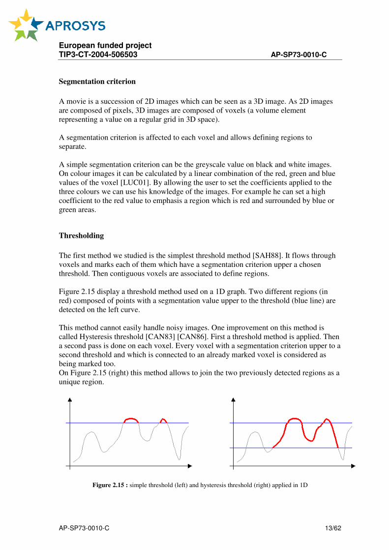
Thresholding
The first method we studied is the simplest threshold method [SAH88]. It flows through
voxels and marks each of them which have a segmentation criterion upper a chosen
threshold. Then contiguous voxels are associated to define regions.
Figure 2.15 display a threshold method used on a 1D graph. Two different regions (in
red) composed of points with a segmentation value upper to the threshold (blue line) are
detected on the left curve.
This method cannot easily handle noisy images. One improvement on this method is
called Hysteresis threshold [CAN83] [CAN86]. First a threshold method is applied. Then
a second pass is done on each voxel. Every voxel with a segmentation criterion upper to a
second threshold and which is connected to an already marked voxel is considered as
being marked too.
On Figure 2.15 (right) this method allows to join the two previously detected regions as a
unique region.
Figure 2.15 : simple threshold (left) and hysteresis threshold (right) applied in 1D

European funded project TIP3-CT-2004-506503 AP-SP73-0010-C
AP-SP73-0010-C 14/62
Watershed
Watershed is a well documented algorithm [BEU92] [JAS02] [ROE99]. It works on 2D
or 3D images gradients which are considered as topographic surfaces (or hyper-surfaces).
To prevent the merging of waters coming from different sources, images are partitioned
into different sets, defining catchment basins and watershed lines.
The segmentation is deduced from catchment basins which should theoretically
correspond to the homogeneous grey level regions of images. Figure 2.16 shows a
watershed method applies to a 1D graph, from the initial drowning to the final
segmentation.
(a)
(b)
(c)
Figure 2.16 : (a) beginning of the drowning (water level in blue), (b) catchment bassins defined (in red),
(c) final segmentation.
2.3.2 Region tracking
The region tracking is only necessary when a 2D detection is performed on all the images
and a region is selected to be tracked on the others. If a 3D detection is applied to all the
images considered as a 3D matrix, a region and its corresponding representations on the
other images are linked during the segmentation.
Many region tracking exist [RAD05] and we decided to use a corresponding method
which calculates the mean segmentation criterion on each detected regions. Then the

European funded project TIP3-CT-2004-506503 AP-SP73-0010-C
AP-SP73-0010-C 15/62
algorithm detects regions which can be linked by comparing the segmentation criterion
means and the superposition percentage of the two regions.
Figure 2.17 : Region tracking on four frames
For example (Figure 2.17) on frame 1 a region is selected by the user. It is projected on
frame 2 and a corresponding region is detected (similar segmentation criterion value and
superposition of regions). Then the process is repeated on each succession of frame until
the movie’s end is reached or a corresponding region is not detected.

European funded project TIP3-CT-2004-506503 AP-SP73-0010-C
AP-SP73-0010-C 16/62
3 Frequency Correlation Criteria
3.1 Introduction
Amongst the extensions provided to ADVISER within this task 7.3.1, a set of criteria
based on analysis of signals in the frequency domain have been added. The primary
purpose is to improve the rating procedure and obtain criteria by analysing the
differences in the frequency domain.
These criteria, analysing in the frequency domain, bring a new series of tools to analyse
and compare curves assuming that a switch to high frquency domain can highlight
characteristics of the signals which are not seen in the time domain. The criteria are
introduced below.
3.2 Theoretical Aspects
3.2.1 Introduction
In this approach, a comparison between different experimental/simulation results is
carried out in
the frequency domain. The discrete fourier transform (DFT) is used to transform original
signals from the time domain.
The formulated criteria are used for comparing two signals. One of the signals (called
“reference signal”) is obtained for example from a “reference” crash test experiment (or a
virtual/simulation test); the other (called “test signal”) is a result of computer simulation
or is obtained from a new experiment. Both signals represent the same physical quantity,
e.g. driver’s head acceleration or seat belt tension.
Some assumptions are made before processing the data:
1. Both signals are sampled with the same sampling frequency.
2. Both signals consist of the same number of samples.
3. Both signals were initially processed in the same way (e.g. both were filtered with
exactly the same filter).
4. Both signals are defined in the time domain.
5. Both signals before comparison were filtered with low-pass filter. The applied
filtering frequency depends on the physical nature of the signal. The signals are
being compared in the frequency domain only below the filtering frequency.
3.2.2 Transformation to the frequency domain
The signal given in the time domain is transformed to the frequency domain. The signal’s
power spectral density (PSD) is calculated using Welch method. The algorithm of
calculations is following:

European funded project TIP3-CT-2004-506503 AP-SP73-0010-C
AP-SP73-0010-C 17/62
1. Signal is padded with trailing zeros to length N, which is the closest power of 2.
As a result of zero padding the same continuous spectrum is obtained, but it is
sampled in different points.
2. The signal given in the time domain is divided into S ( S = 2M
−1, M is user-
defined) overlapping segments of equal width K = N / 2M-1
. The subsequent
segments are shifted by half of their width, as it is illustrated in the figure below.
Figure 3.1. Signal divided into overlapping segments.
3. The Hanning window is applied to each segment. The widowing consists in
multiplication of i-th sample (xi) with i-th coefficient of the window (hi): yi = hi•xi
, i = 1, …,K
4. The coefficients (hi) of K-point Hanning window are given by:
(1)
The H value (which is necessary later on) is calculated as the sum of squares of
window coefficients:
(2)
5. The discrete Fourier transform (DFT) is applied to each segment of the signal.
The number of samples is a power of 2, so the fast Fourier transform (FFT)
algorithm can be applied. Prior to FFT calculation (but after the windowing) the
signal in each segment is zero padded to length N. This way the obtained
frequency resolution is the same as the FFT resolution of signal not divided into
segments. Discrete Fourier transform of N-point signal {yi} is defined as:
(3)
The l-th sample of FFT corresponds to frequency fl, given by:

European funded project TIP3-CT-2004-506503 AP-SP73-0010-C
AP-SP73-0010-C 18/62
(4)
where fs is the sampling frequency.
A single point of discrete Fourier transform is a complex number:
(5)
6. The power spectrum of signal is calculated. It is defined as a square of magnitude
of Fourier transform, divided by the number of samples N and by the sum of
squares of window coefficients H divided by N:
(6)
7. The power spectrum is symmetrical about the Nyquist frequency (Nyquist
frequency is equal half of the sampling frequency fs). Therefore, only the first half
of power spectrum, i.e. frequency range from 0 to fs/2 is considered (the power is
multiplied by 2). The power spectra for all S segments are averaged and then
divided by sampling frequency fs, to obtain the power spectral density (PSD):
(7)
3.2.3 Cross spectral density
Unlike the real-valued PSD the cross spectral density (CSD) is a complex function. To
estimate the CSD of two equal length signals x and y the Welch method (described
above) is applied to obtain FFT of the signal x and FFT of signal y. The CSD is
calculated as the FFT of signal x and conjugate of the FFT of y. The sectioning and
windowing of x and y is handled in the same way as in the method described above.
(8)
It is known that cross spectral densities can be obtained as Fourier transforms of cross-
correlations functions of signals x and y. The cross spectral densities of signals x and y
are denoted as SXY(f) (CSD is a function of frequency f).
The signals considered here are characterized by large PSD value corresponding to low
frequencies and small value for higher frequencies. The signal power associated to high
frequencies is relatively small. Higher frequency components cannot be, however,

European funded project TIP3-CT-2004-506503 AP-SP73-0010-C
AP-SP73-0010-C 19/62
neglected during signal analysis, because they are responsible for peaks visible in the
time domain. It can be easily observed in the following example. The Figure 3.2 shows
signal x, for which DFT was calculated. The high frequency samples responsible for only
5% of power were set to zero.
Next, the inverse discrete Fourier transform (IDFT) was calculated. The obtained signal
x%
is also presented in the figure. The comparison of x with x%
shows, that high
frequencies are responsible for amplitudes of peaks in time domain.
Figure 3.2. Signal comparison
There are great differences between values Xl corresponding to low and high frequencies.
That is why it is sometimes convenient to present the PSD values in decibels, calculated
as follows:
(9)
The Figure below presents an example of signal in the time domain (x(t)), power spectral
density of this signal (X(f)) and power spectral density in decibels (XdB
(f)).
Figure 3.3. Signal in time domain, PSD and PSD in decibels
3.2.4 Other approaches

European funded project TIP3-CT-2004-506503 AP-SP73-0010-C
AP-SP73-0010-C 20/62
PSD and CSD are basic elements for the evaluation of the proposed criteria. Some other
tools (such as approximation of the PSD by polynomial or splines) are used. The
referenced reports (from VITES project) give all mathematical details related to those
criteria.
3.3 Proposed criteria
3.3.1 Signals power comparison
Two signals x(t) and y(t) can be transformed into frequency domain and their power
spectral densities can be calculated, as it is described in section 2.2.2. As it was assumed,
the power spectral densities are being compared only in the frequency band from 0 to
filtering frequency ff. Discrete PSD contains L samples (the L value depends on sampling
frequency and on filtering frequency). The Px value, which is proportional to signal X(f)
power, can be calculated as follows (for Y(f) the formula is analogous):
(10)
Powers of signals can be used for their comparison. The following formula of
quantitative signals comparison was proposed:
(11)
3.3.2 Signals power comparison in bands
All the analyzed frequency range can be divided into several bands. Power associated
with each band can be calculated using equation (10). Power in each band can be then
compared separately. For each band the partial score can be calculated using (11).
This way, instead of single score we obtain as many scores, as many bands we have. The
partial scores can be then averaged to obtain single value. If for some reason similarity of
signals in selected frequency band is more important than in other bands, then it is
possible to consider this fact by using appropriate weight coefficient during calculation of
average score. During test calculations it was found, that the number of frequency bands
should be greater than four.
This criterion can also be used repeatedly. The number of frequency bands can be
gradually increased.

European funded project TIP3-CT-2004-506503 AP-SP73-0010-C
AP-SP73-0010-C 21/62
3.3.3 Frequency comparison per power level
The basis of this criterion is comparison of frequencies below which certain percent of
total signal power is included. The percentage of signal power below selected frequency
fk can be calculated as follows:
(12)
The Px value is defined by equation (10).
Let fx denote the frequency below which certain percent of total power of signal X(f) is
included, and let fy denote frequency below which the same percent of total power of
signal Y(f) is included. The following formula of quantitative signals comparison was
proposed:
(13)
Symbol fref denotes reference frequency range. It was chosen to be a half of analyzed
frequency range, defined by the filtering frequency:
(14)
During calculations equation (13) can be replaced with similar one, using X(f) and Y(f)
sample indices rather than sample frequencies (in this case information about sampling
frequency is not needed). Frequencies fx and fy should be replaced with respective
indices kx and ky. In equation (14) the filtering frequency ff should be replaced with
number of points in analyzed spectrum – L. Equation (13) can be then rewritten as:
(15)
Test calculations proved that reasonable results are obtained when frequencies
corresponding to 50%, 75%, 90%, 95% and 99% of signal power are being compared.
For each power level a partial score is calculated.
3.3.4 Maximal Signals power densities comparison
In this criterion, the maximal values Xmax and Ymax in power spectral densities of signal X(f)
and Y(f) being compared, as well as corresponding to them indices kx and ky are sought for.
Two scores that enable values and frequencies comparison were proposed:
(16)

European funded project TIP3-CT-2004-506503 AP-SP73-0010-C
AP-SP73-0010-C 22/62
(17)
The proposed method of scoring can be classified as a point criterion generating two
partial scores. Signal power spectral densities serve as input data.
3.3.5 Comparsion of PSD approximations (by a polynomial)
The considered power spectral densities X(f) and Y(f) can be approximated by
polynomials. Analytical formulae describing approximating polynomials can be treated
as an analytical description of PSD. For higher frequencies the PSD values are close to
zero, which is why the polynomial approximation is made only for lower frequencies.
Let fx90
and fy90
denote frequencies, below which 90% of signals X(f) and Y(f) total power
is included. Power spectral densities of both signals are approximated by fourth degree
polynomials in the frequency range from 0 to fap and fap is defined as follows:
(18)
Let ax and ay denote corresponding coefficients of polynomials approximating power
spectral densities X(f) and Y(f). The following score, enabling for coefficient comparison
was proposed:
(19)
The proposed criterion generates five partial scores (there are five coefficients of 4th
degree polynomial). It should be emphasized that coefficients of approximating
polynomials must be calculated separately for each pair of compared signals, because
each time the value fap is different.
3.3.6 Comparsion of PSD approximations (by a spline)
Same approach as for polynomial coefficients, but since there are many coefficients, only
the mean value of those coefficients is considered.

European funded project TIP3-CT-2004-506503 AP-SP73-0010-C
AP-SP73-0010-C 23/62
3.3.7 Comparison of PSD local extrema
If we denote Xsp(f) and Ysp(f) the spline approximations of the signals to compare (X and
Y), then in the proposed method of signals comparison the maxima found in Ysp(f) are
being compared with the maxima found in Xsp(f). Then, the same procedure is applied to
the minima. The values, as well as the frequencies of local extrema are being compared.
The first local maximum of Xsp(f) is compared with the first local maximum of Ysp(f); the
second is compared with the second, etc. For each pair of local maxima/minima Xm and Ym
(and corresponding to them indices kx and ky) two scores were proposed:
(20)
3.3.8 Comparsion of PSD slopes
The similarity of Xsp(f) and Y sp(f) can be evaluated by comparison of power spectral
density slope on the right hand side of the global maximum. The slope (the magnitude of
the first derivative of spline function) is varying. The maximal values of slope are being
compared.
Let dx and dy denote maximal slopes (the values of the first derivatives) of PSD on the
right hand side of global maximum for signals Xsp(f) and Y sp(f), respectively. The
following score was proposed:
(21)
3.3.9 Comparsion of differences between signals and their approximations
There are differences between power spectral density in decibels XdB(f) and their spline
approximation Xsp(f). The smoother the PSD is, the smaller the differences are. The
measure of difference between PSD and its spline approximation can be defined as
follows:
(22)

European funded project TIP3-CT-2004-506503 AP-SP73-0010-C
AP-SP73-0010-C 24/62
In the above equation N denotes the number of spline segments, M is the number of
discrete PSD points corresponding to each spline segment and XdB(j) is the j-th point of
discrete PSD.
Examples of signals with small and large value of r are presented below:
Figure 3.4. Signals with small (left side) and large (right side) value of r.
The similarity of XdB (f) and YdB(f) can be evaluated by comparison of rx and ry measures.
The following score was proposed:
(23)
3.3.10 Comparsion of signals correlation as a function of the frequency
Other characteristics can be formulated basing on comparison of the signals correlation
for different frequencies f. As a measurement quotient the magnitude squared coherence
function between signals x and y is used, defined as:
(24)
First the PSD of signals X and Y are estimated and the cross spectral density function
SXY(f) is evaluated in turn. Using these results the quotient is evaluated.
Two criteria for evaluation of signals correlations are proposed. The first criterion
consists in evaluation of signals correlation in the frequency interval [f1,f2]. The sum of
subinterval lengths in the interval [f1,f2] is found where C < C1 or separately C > C2.
Two scores are defined. The first is:
(25)

European funded project TIP3-CT-2004-506503 AP-SP73-0010-C
AP-SP73-0010-C 25/62
where LC>C2 is number of discrete frequencies from the frequency range [f1, f2], for which
C>C2 , and Lf1 f 2 is number of all discrete frequencies from the range [f1, f2]. This criterion
indicates percentage of frequency interval [f1, f2] for which signals are strongly correlated.
The analogous criterion, but serving as a quotient measuring the percentage of frequency
interval [f1, f2] where signals are nearly not correlated is given by the formula:
(26)
where LC>C2 is number of discrete frequencies from the frequency range [f1,f2], for which
C < C1. The values of f1 and f2 can be taken arbitrarily. However, the default application
of this criterion is proposed in three variants:
1. f1=0 and f2 is upper bound of frequency analysis range (resulting form the cutting
frequency of the filter)
2. In two frequency intervals with equal lengths, resulting from division the
frequency analysis range into two intervals
3. Ditto, but with division of frequency analysis range into three intervals with equal
lengths.
3.4 ADVISER Frequency Correlation features
3.4.1 Criteria Implemented
A generic keyword called “signal” has been choosen to implement in ADVISER all the
criteria presented above. The syntax is as follows :
filexy[a=a.xy]
filexy[b=b.xy]
param[3,1,1,1]
signal[c=~spc(a,b)]
Here, 2 curves (a and b, initially in the time domain) are compared using the ~spc
operator (signal power comparison) and the comparison score is returned in c. The param
command is used to define some options of the ~spc operator.
The selected operators available are :
- ~spc : signals power comparison
- ~spb : signals power comparison in bands
- ~fcp : frequency comparison per level
- ~msp : maximal signal power densities comparison
- ~pol : comparsion of polynomial coefficients
- ~spl : comparsion of spline coefficients
- ~lep : local extrema position comparison
- ~slo : power spectral density slope comparison

European funded project TIP3-CT-2004-506503 AP-SP73-0010-C
AP-SP73-0010-C 26/62
- ~sad : comparison between signals and their approximations
- ~scr : comparison of signal correlation (frequency)
3.4.2 Example
Example 1 : Accelerometer signal from dummy head.
The two curves displayed below are compared with the new frequency-based criteria.
Figure 3.5. First Example
~spc
param[3,1000,3,5]
signal[@S1=~spc(A,B)] Signal Power comparison value score = 7.88297125E+01
~spb
param[4,1000,3,10,5] (5 frequency bands are considered)
signal[@S1=~spb(A,B)] Signal Power score (band 1) = 7.76973075E+01
Signal Power score (band 2) = 4.85957367E+01
Signal Power score (band 3) = 3.87843470E+01
Signal Power score (band 4) = 5.30379918E+00
Signal Power score (band 5) = 8.88132998E+00
~fcp
signal[@S1=~fcp(A,B)] Signal Frequency comparison score 1 = 9.75903614E+01
Signal Frequency comparison score 2 = 9.75903614E+01
Signal Frequency comparison score 3 = 1.00000000E+02
Signal Frequency comparison score 4 = 9.75903614E+01
Signal Frequency comparison score 5 = 7.10843373E+01

European funded project TIP3-CT-2004-506503 AP-SP73-0010-C
AP-SP73-0010-C 27/62
~msp
signal[@S1=~msp(A,B)] Maximal Power Spectral Densities Value score = 1.00000000E+02
Maximal Power Spectral Densities Frequency score = 9.28962976E+01
~pol
signal[@S1=~pol(A,B)] Polynomial Coefficient comparison score 1 = 9.28920503E+01
Polynomial Coefficient comparison score 2 = 0.00000000E+00
Polynomial Coefficient comparison score 3 = 3.26722791E+01
Polynomial Coefficient comparison score 4 = 0.00000000E+00
Polynomial Coefficient comparison score 5 = 3.82153037E+01
~spl
signal[@S1=~spl(A,B)] Spline Coefficients comparison scores :
- Score 1 = 9.98314662E+01
- Score 2 = 9.54116074E+01
- Score 3 = 9.93079024E+01
- Score 4 = 9.43316628E+01
- Score 5 = 9.02492893E+01
...
- Score 38 = 2.77655545E+01
- Score 39 = 2.08537495E+01
- Score 40 = 0.00000000E+00
~lep
param[4,1000,3,10,6] (up to 6 extrema are considered)
signal[@S1=~lep(A,B)] Local Extrema Position comparison scores :
Frequency score for local extremum 1 = 9.81915160E+01
Frequency score for local extremum 2 = 2.84253923E+01
Frequency score for local extremum 3 = 0.00000000E+00
Frequency score for local extremum 4 = 0.00000000E+00
Frequency score for local extremum 5 = 0.00000000E+00
Frequency score for local extremum 6 = 0.00000000E+00
Value score for local extremum 1 = 9.91514837E+01
Value score for local extremum 2 = 8.43523763E+01
Value score for local extremum 3 = 0.00000000E+00
Value score for local extremum 4 = 0.00000000E+00
Value score for local extremum 5 = 0.00000000E+00
Value score for local extremum 6 = 0.00000000E+00
~slo
signal[@S1=~slo(A,B)] Power Spectral Density Slope comparison score = 9.60225758E+01

European funded project TIP3-CT-2004-506503 AP-SP73-0010-C
AP-SP73-0010-C 28/62
~sad
signal[@S1=~sad(A,B)] Signal vs. Approximation comparison score = 8.41526328E+01
~scr
signal[@S1=~scr(A,B)] Signals correlation comparison - max coherence score = 1.00000000E+02
Signals correlation comparison - min coherence score = 9.87951807E+01
Example 2 :
Figure 3.6. Second Example
~spc
param[3,1000,3,5]
signal[@S1=~spc(A,B)] Signal Power comparison value score = 6.32884161E+01
~spb
param[4,1000,3,10,5]
signal[@S1=~spb(A,B)] Signal Power score (band 1) = 6.55626818E+01
Signal Power score (band 2) = 1.42581300E+01
Signal Power score (band 3) = 2.03645588E+00
Signal Power score (band 4) = 2.66515443E+00
Signal Power score (band 5) = 5.66535337E+00
~fcp
signal[@S1=~fcp(A,B)] Signal Frequency comparison score 1 = 9.95121951E+01
Signal Frequency comparison score 2 = 9.80487805E+01
Signal Frequency comparison score 3 = 9.36585366E+01
Signal Frequency comparison score 4 = 8.78048780E+01
Signal Frequency comparison score 5 = 0.00000000E+00
European funded project TIP3-CT-2004-506503 AP-SP73-0010-C
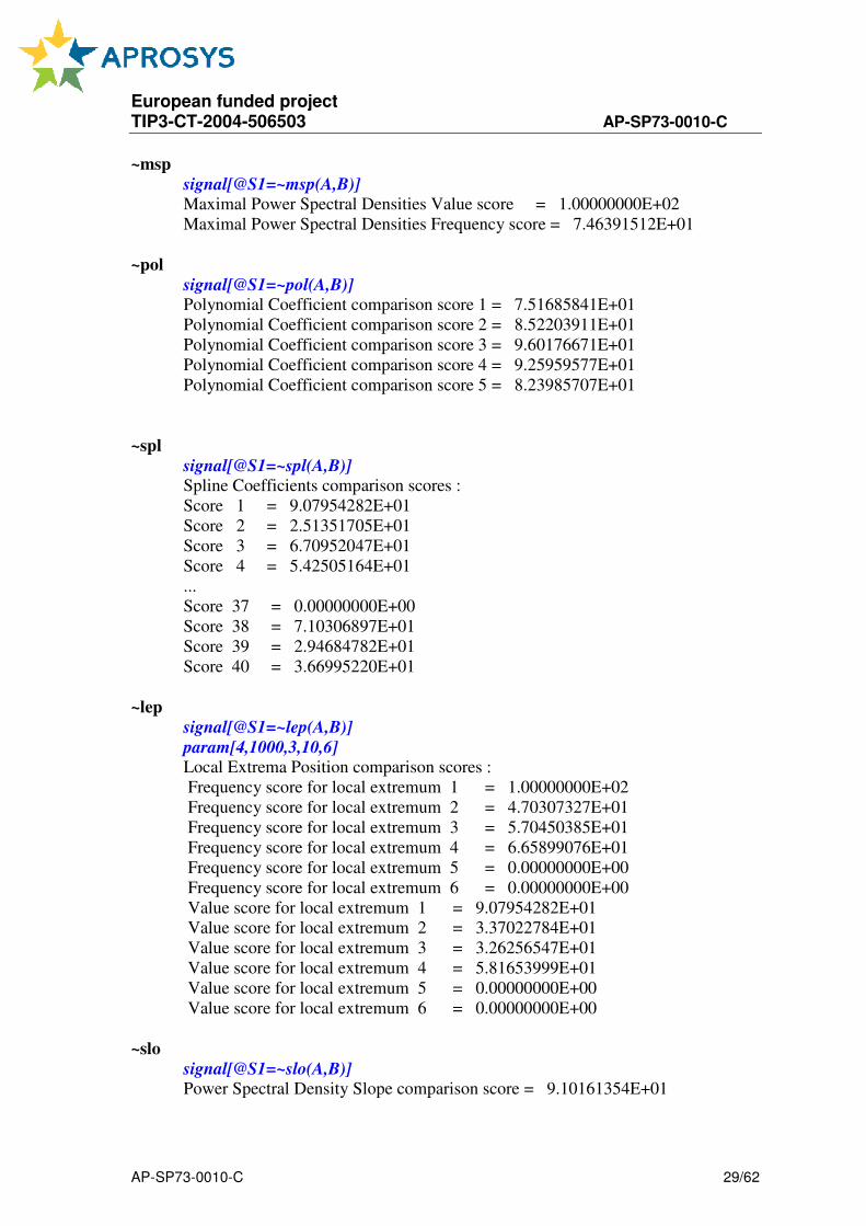
AP-SP73-0010-C 29/62
~msp
signal[@S1=~msp(A,B)] Maximal Power Spectral Densities Value score = 1.00000000E+02
Maximal Power Spectral Densities Frequency score = 7.46391512E+01
~pol
signal[@S1=~pol(A,B)] Polynomial Coefficient comparison score 1 = 7.51685841E+01
Polynomial Coefficient comparison score 2 = 8.52203911E+01
Polynomial Coefficient comparison score 3 = 9.60176671E+01
Polynomial Coefficient comparison score 4 = 9.25959577E+01
Polynomial Coefficient comparison score 5 = 8.23985707E+01
~spl
signal[@S1=~spl(A,B)] Spline Coefficients comparison scores :
Score 1 = 9.07954282E+01
Score 2 = 2.51351705E+01
Score 3 = 6.70952047E+01
Score 4 = 5.42505164E+01
...
Score 37 = 0.00000000E+00
Score 38 = 7.10306897E+01
Score 39 = 2.94684782E+01
Score 40 = 3.66995220E+01
~lep
signal[@S1=~lep(A,B)]
param[4,1000,3,10,6]
Local Extrema Position comparison scores :
Frequency score for local extremum 1 = 1.00000000E+02
Frequency score for local extremum 2 = 4.70307327E+01
Frequency score for local extremum 3 = 5.70450385E+01
Frequency score for local extremum 4 = 6.65899076E+01
Frequency score for local extremum 5 = 0.00000000E+00
Frequency score for local extremum 6 = 0.00000000E+00
Value score for local extremum 1 = 9.07954282E+01
Value score for local extremum 2 = 3.37022784E+01
Value score for local extremum 3 = 3.26256547E+01
Value score for local extremum 4 = 5.81653999E+01
Value score for local extremum 5 = 0.00000000E+00
Value score for local extremum 6 = 0.00000000E+00
~slo
signal[@S1=~slo(A,B)]
Power Spectral Density Slope comparison score = 9.10161354E+01

European funded project TIP3-CT-2004-506503 AP-SP73-0010-C
AP-SP73-0010-C 30/62
~sad
signal[@S1=~sad(A,B)] Signal vs. Approximation comparison score = 2.91140308E+01
~scr
signal[@S1=~scr(A,B)] Signals correlation comparison - max coherence score = 0.00000000E+00
Signals correlation comparison - min coherence score = 0.00000000E+00

European funded project TIP3-CT-2004-506503 AP-SP73-0010-C
AP-SP73-0010-C 31/62
4 Footprint Criteria for barriers
4.1 Introduction
In the deliverable report D713B (Report on frontal impact barriers), a section is dedicated
to investigations on footprint methods for assessing barrier models results. These
methods have been implemented in ADVISER as standard criteria.
The objective of these criteria based on footprints is to offer advanced ratings going
further than the classical “global force measures” and taking into account the local
deformation patterns.
4.2 Review of some footprint methods
Please refer to the deliverable D713B for the complete description of these methods and
examples of their application.
4.2.1 Footprint methods based on load cell wall measurements
The main footprint criteria are based upon the analysis of load cell wall forces measured
at the rear of a barrier (either numerical or experimental) in a frontal impact.
The load cell wall consists in a set of Nrow x Ncol data channels. Each data channel
represents the record of the load cell force versus time. Nrow is the number of rows
(vertically) and Ncol the number of columns (horizontally) of the load cell wall.
Two main families of footprint criteria are investigated here: Homogeneity criteria and
Performance criteria.
Homogeneity criteria
This first family of criteria can be used to assess the vehicle performance, to quantify the
effectiveness of a car in meeting the requirements for frontal impact compatibility, but
also to validate a numerical barrier in comparison to an experimental barrier.
The data is first processed as follows:
1. Standard data set:
Each channel of the load cell wall is filtered with a CFC60 filter and will be denoted
by Fi,j, where i denotes the row and j denotes the column.
2. Smoothed data set:

European funded project TIP3-CT-2004-506503 AP-SP73-0010-C
AP-SP73-0010-C 32/62
The standard data set is spatially smoothed to form a new channel array, in which
every channel is the average of four channels from the standard data set.
If a new channel is denoted sFi,j, it is computed as:
)(4
11,1,11,,, −−−− +++= jijijijijis FFFFF
If any channel from the standard data set does not exist (for example if i=1 or j=1),
then it is substituted by the value 0 and the denominator (for the computation of sFi,j)
is reduced.
3. Smoothed footprint array:
The maximum value against time (denoted by sfi,j) of each channel of the smoothed
data set is computed to compose the smoothed footprint array.
The various homogeneity criteria are then computed as follows :
Target Load Level (L)
It is defined as the mean of the peak cell forces (from the smoothed data set). It is
equal to the sum of the peak cell forces divided by the number of cells of the load cell
wall:
colrow
N
i
N
j
jis
NN
f
L
row col
×=∑∑
= =1 1
,
Overall Cell Homogeneity (Hcl)
It describes the variability of load peaks between individual cells in the footprint. It is
defined as:
colrow
N
i
N
j
jis
clNN
fL
H
row col
×
−
=∑∑
= =1 1
2
, )(
Vertical Homogeneity (Hr)
It describes the variability of the mean value (of load peaks) for each row and
provides an indication of the vertical force distribution. It is defined as:

European funded project TIP3-CT-2004-506503 AP-SP73-0010-C
AP-SP73-0010-C 33/62
row
N
i
N
j
jis
col
rN
fN
L
H
row col
∑ ∑= =
−
=1
2
1
,
1
Horizontal Homogeneity (Hc)
It describes the variability of the mean value (of load peaks) for each column and
provides an indication of the horizontal force distribution. It is defined as:
col
N
j
N
i
jis
row
cN
fN
L
H
col row
∑ ∑= =
−
=1
2
1
,
1
Total Homogeneity (Ho)
A total homogeneity criterion can defined as:
crcl cHbHaHH ++=0
where: a, b and c are constants defined by the user.
Performance criteria
The compatibility of vehicles to protect their occupants, the pedestrians as well as
limiting damage to the other vehicles can be controlled by a vehicle-structure interaction.
Performance criteria are a way to quantify the structural interaction.
Each channel of the load cell wall is denoted by Fi,j, where i denotes the row and j
denotes the column. The height of a load cell (from the ground to the centre of the load
cell) is denoted by hi, where i denotes the row.
The two performance criteria are computed as follows :
1. Height of Force (HOF):
It represents the sum of the load cell forces multiplied by their respective height from
ground, divided by the total force (sum of all load cell forces). It is computed for each
time step.
It is defined as:

European funded project TIP3-CT-2004-506503 AP-SP73-0010-C
AP-SP73-0010-C 34/62
∑∑
∑∑
= =
= =
×
=row col
row col
N
i
N
j
ji
N
i
N
j
iji
F
hF
tHOF
1 1
,
1 1
,
)(
2. Average Height of Force (AHOF):
The height of force is averaged using the total force from each time step as a
weighting function. It is defined as:
∑
∑
=
=
×
=final
final
t
t
t
t
tF
tFtHOF
AHOF
0
0
)(
)()(
4.2.2 Footprint methods based on barrier deformation
This family of footprint methods can be used to assess the protection of the vehicle
environment.
These criteria are based on the deformation of the barrier. Indeed the shape of the barrier
after a crash gives information about front unit homogeneity as a combination of the
force distribution and the pushing surface.
As for the load cell wall, the front face of the barrier can be "cut" in several surfaces, for
which we need to get three main parameters: the average height of the surface, the
average deformation of the surface and the surface area.
- Zi represents the average height of the surface i (in mm).
- Xi represents the average deformation of the surface i (in mm).
- Si represents the surface of the surface i (in cm²).
- Nsurf represents the number of surfaces.
These values are obtained at the end of the crash (using barrier digitization for
experiments or the final nodal displacement for simulations).

European funded project TIP3-CT-2004-506503 AP-SP73-0010-C
AP-SP73-0010-C 35/62
Partner Protection Assessment (PPA) criteria
The various PPA criteria are expressed as follows:
1. Maximum Deformation (Dmax):
It corresponds to the maximum value of the barrier deformation. It is defined as:
surfi NiXD ,1)max(max ==
2. Height of Maximum Deformation (Z(Dmax)):
It corresponds to the height for which the barrier deformation is maximum.
3. Total Volume Deformed (V):
It is defined as:
∑=
×=surfN
i
ii SXV1
4. Partner Protection Assessment of Deformation (PPAD):
The aim of this criterion [UTA04, DEL05] is to provide the user an aggressiveness
scale of the vehicle. It is defined as:
∑=
×
×
=
surfN
i
iii S
X
X
Z
ZR
1
2
lim
4
lim
55.0
10
52.0RPPAD =
This criterion gives values from 1 to 12:
� 1 means the vehicle is non aggressive
� 12 means the vehicle is aggressive
The drawback of this criterion is that it uses two limit factors (Xlim and Zlim), which
must be adapted to the kind of cars the user want to protect.
Default values are:
Zlim = 420 mm corresponding to the average longitudinal height in Europe.
Xlim = 300 mm.

European funded project TIP3-CT-2004-506503 AP-SP73-0010-C
AP-SP73-0010-C 36/62
4.3 Implementation in ADVISER
The footprint criteria presente above have been implemented in ADVISER through a new
keyword called "footprint".
Four scalar can be extracted, 3 using forces measured on a load cell wall (rear of the
barrier) and 1 based on barrier deformation (measured on the front of the barrier):
1. Height of Force (operator "hof"):
7 input parameters are needed :
1) Number of load cells (horizontal)
2) Number of load cells (vertical)
3) Type of input (0 for XY curves - 1 for LST curves)
4) Filtering frequency (in Hz)
5) Scale factor to have curves in 1/s (1000 if curves are given in ms)
6) Minimum height of the barrier (from the ground)
7) Maximum height of the barrier (from the ground)
1 argument is needed :
One ASCII curve (XY or LST) per cell (representing total force measured on the
cell) must exist. The argument given to the operator is the rootname for curves (curves
are then read as "rootname_i_j.xy" where i is the horizontal index of the cell and j its
vertical index)
1 ouput is produced :
a curve called "height of force"
The syntax to use is :
param[7,6,16,0,60,1000,50,800]
footprint[a=~hof(TEST_FOOTPRINT/BAFW1T_LOAD_CELL)]
2. Average Height of Force (operator "ahof"):
7 input parameters are needed :
1) Number of load cells (horizontal)
2) Number of load cells (vertical)
3) Type of input (0 for XY curves - 1 for LST curves)
4) Filtering frequency (in Hz)
5) Scale factor to have curves in 1/s (1000 if curves are given in ms)
6) Minimum height of the barrier (from the ground)
7) Maximum height of the barrier (from the ground)

European funded project TIP3-CT-2004-506503 AP-SP73-0010-C
AP-SP73-0010-C 37/62
1 argument is needed :
One ASCII curve (XY or LST) per cell (representing total force measured on the
cell) must exist. The argument given to the operator is the rootname for curves (curves
are then read as "rootname_i_j.xy" where i is the horizontal index of the cell and j its
vertical index)
1 ouput is produced :
Average height of force (see manual for its formulation)
The syntax to use is :
param[7,6,16,0,60,1000,50,800]
footprint[a=~ahof(TEST_FOOTPRINT/BAFW1T_LOAD_CELL)]
3. Homogeneity criteria (operator "hom"):
8 input parameters are needed :
1) Number of load cells (horizontal)
2) Number of load cells (vertical)
3) Type of input (0 for XY curves - 1 for LST curves)
4) Filtering frequency (in Hz)
5) Scale factor to have curves in 1/s (1000 if curves are given in ms)
6) Scale factor for the computation of the total homogeneity
7) Scale factor for the computation of the total homogeneity
8) Scale factor for the computation of the total homogeneity
1 argument is needed :
One ASCII curve (XY or LST) per cell (representing total force measured on the
cell) must exist. The argument given to the operator is the rootname for curves (curves
are then read as "rootname_i_j.xy" where i is the horizontal index of the cell and j its
vertical index)
5 ouputs are produced :
1) Target Load Level
2) Overall Cell Homogeneity
3) Vertical Homogeneity
4) Horizontal Homogeneity
5) Total Homogeneity
The syntax to use is :
param[8,6,16,0,60,1000,1,1,1]
footprint[a=~hom(TEST_FOOTPRINT/BAFW1T_LOAD_CELL)]

European funded project TIP3-CT-2004-506503 AP-SP73-0010-C
AP-SP73-0010-C 38/62
4. Partner Protection Assessment (operator "ppa")
2 input parameters are needed :
1) Limit for deformation (300 mm by default)
2) Limit for height ( 420 mm by default)
3 arguments are needed :
1) Data file containing the deformation (actually a displacement) measured on
the different surfaces of the front of the barrier (in mm)
2) Data file containing the height of each surface (in mm)
3) Data file containing the surface of each surface (in cm²)
7 ouputs are produced :
1) Average Depth of Deformation
2) Average Height of Deformation
3) Maximum Deformation
4) Height at Maximum Deformation
5) Total Volume Deformed
6) Aggressiveness Scale (R)
7) Partner Protection Assessment of Deformation (PPAD)
The syntax to use is :
param[2,300,420]
footprint[a=~ppa(ppa_deformation.data,ppa_height.data,ppa_surface.data)]
4.4 Application of the footprint criteria
The criteria introduced in the previous section can be applied either to a set of numerical
responses or to the results of an experiment. Comparison of footprint criteria can then be
used to validate the barrier model.
These footprint methods have been applied to the RADIOSS TRL barrier for a full
impact with a rigid wall at 56 km/h. The load cell wall of TRL barrier model is composed
of 6 rows and 16 columns, i.e. 96 cells. So we have 96 channels as input data, which are
defined as:
TRL_MODEL_LOAD_CELL_i_j.xy (where i=1 to 6 and j=1 to
16)

European funded project TIP3-CT-2004-506503 AP-SP73-0010-C
AP-SP73-0010-C 39/62
4.4.1 Graphical Illustration of the footprint criteria
To illustrate this example, we have created tables (using the Evaluation Module of
ADVISER ) representing the load cell wall (see Figure 4.1: each test corresponds to a
row of the cell wall and each property to a column). Each element of the table represents
a cell of the rear wall of the TRL barrier.
Figure 4.1: ADVISER Evaluation module – Table representing the load cell wall
From this table we are able to compute the cell forces at different times and display it
with the ColorMap Module (Figure 4.2), in order to see the evolution of the forces
distribution against time:
Figure 4.2: ADVISER ColorMap module – Load cell forces [kN] at t= 23 ms
For the homogeneity criteria, each channel of the standard data set (initial array) is
filtered at CFC60 and then smoothed to compose the smoothed data set.
European funded project TIP3-CT-2004-506503 AP-SP73-0010-C
AP-SP73-0010-C 40/62
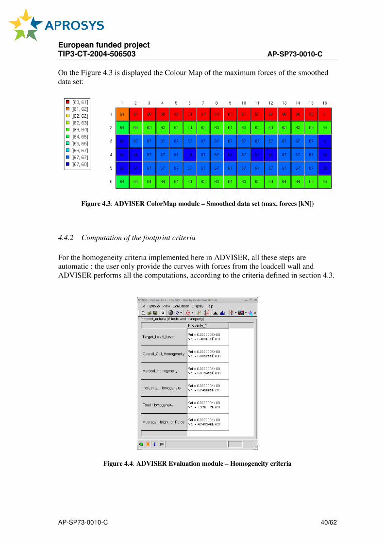
On the Figure 4.3 is displayed the Colour Map of the maximum forces of the smoothed
data set:
Figure 4.3: ADVISER ColorMap module – Smoothed data set (max. forces [kN])
4.4.2 Computation of the footprint criteria
For the homogeneity criteria implemented here in ADVISER, all these steps are
automatic : the user only provide the curves with forces from the loadcell wall and
ADVISER performs all the computations, according to the criteria defined in section 4.3.
Figure 4.4: ADVISER Evaluation module – Homogeneity criteria

European funded project TIP3-CT-2004-506503 AP-SP73-0010-C
AP-SP73-0010-C 41/62
5 Extension of Rating Methods
5.1 Signal Rating
After completion of the VITES project TNO started to systematically rate MADYMO
dummy models & human models. The primary objective of these efforts was to quantify
model accuracy while a second objective was to use ADVISER rating for model
parameter estimation.
In the VITES project dummy models have been rated using dummy certification data and
some sled tests [PUP01]. The current validation database of the MADYMO Hybrid III
contains over 4000 signals, where for each signal the shape, peak amplitude and peak
timing, and where applicable the derived injury criteria, are rated. The handling of such
large sets of data calls for automated data post-processing, as it can no longer be expected
that all signal output is inspected visually on a regular basis.
Parameter estimation leads to additional requirements for the rating methods applied. In
particular it is desirable that the rating values do not show discontinuities when model
parameters are changed. Furthermore, the optimum of such criteria should provide an
unbiased estimation of the parameter at hand, and local minima should be avoided.
Below some requirements and solutions are presented. Not all these developments were
made as part of the APROSYS project.
5.1.1 Associative Scalar Scores
To compare two scalar values, for example peak values or injury values, the following
expression is commonly used:
−−=
exp
simexp1,0maxcrit (5.1)
In this document, the above method will be called the Relative Error Method (REM). The
Relative Error Method is not associative: crit(exp, sim) ≠ crit(sim, exp). The REM score
drops off faster with over-prediction than with under-prediction: an over-prediction by a
factor of 2 results in a much lower score than an under-prediction by a factor of two. The
rating score drop-off of the REM method is shown in figure 5.1, where a log2 scale is
used for the abscissa to show ratios that are powers of two on a linear scale:

European funded project TIP3-CT-2004-506503 AP-SP73-0010-C
AP-SP73-0010-C 42/62
As a result, applying this formula to optimize a model for a set of tests tends to result in a
model that systematically under-predicts test outcomes. Since this under-prediction is
undesirable for the dummy models the following calculation is proposed, called the
Factor Method:
( )( )22 sim,expmax
simexp,0maxcrit
⋅= (5.2)
The Factor Method (FM) calculates the correlation between exp and sim, resulting in a
value that lies between 0 and 1. This expression is associative: crit(exp, sim) =
crit(sim,exp). For small differences between exp and sim the results are identical or
almost identical to the results of the REM. However, it is important to realize that for
over-predictions the FM calculates values that do not drop off faster than for under-
prediction, as is the case with the REM, see figure 5.2.
0
0.2
0.4
0.6
0.8
1
1.2
-1.5 -1 -0.5 0 0.5 1 1.5
log2(sim/exp)
sco
re
Figure 5.1: REM method score drop-off (log2 scale).
0
0.2
0.4
0.6
0.8
1
1.2
-1.5 -1 -0.5 0 0.5 1 1.5
log2(sim/exp)
sco
re
Figure 5.2: Rating score drop off for the FM method (log2 scale)

European funded project TIP3-CT-2004-506503 AP-SP73-0010-C
AP-SP73-0010-C 43/62
For example, for an over-prediction of 100% (log2(sim/exp)=1) the FM rating results in a
score of 0.5, whereas the REM score will have dropped to 0. When optimizing a target
function using the FM, the solution will not tend to under-predict most tests as it does
with the REM method. The Factor Method can be used to compare two scalar values, for
example a peak amplitude or the timing of the peak amplitude.
The implementation of REM in an algorithm has to take care of a special situation:
1) when the values of exp and sim both are equal to zero. In this case, the divisor
in formula 1 becomes zero and it is not possible to calculate the criterion. An
example of a situation in which this occurs is in the calculation of a peak
timing score in a situation where the largest amplitude occurs at t=0.
2) A second example in which problems occur is that in which both signals that
are compared are equal to zero for the entire interval.
The algorithm handles this by first comparing the two scalars, before computation of the
rating score according to formula 5.1. If the two values are equal, a rating score of 5.1
(perfect correlation) is returned immediately. In this way, if two zeros are compared, then
the result of the rating calculation is 1.
5.1.2 Associative Signal Scores
Comparing experiments with simulations requires examining entire time-histories, i.e.
comparing two vectors. A criterion is proposed here that is a combination of the Factor
Method (formula 5.2) and the RMS Addition method (formula 5.5). It is called the WIFac
method, which stands for Weighted Integrated Factor method. Its formulation is as
follows:
( ) ( )( )
( )∑
∑
⋅−⋅
−=22
2
22
22
][,][max
][,][max
][][,0max1][,][max
1ngnf
ngnf
ngnfngnf
crit (5.3)
Effectively this is formula 5, where crit has been replaced by formula 5.2, the weight
factor has been chosen as the square of the absolute maximum of the function values, and
the summation has been replaced by integration.
Formula 5.2 has been included to get a consistent set of criteria definitions. The weight
factor has been chosen similar to the function itself.
Note that TNO previously proposed to use a linear weighting of the scalar scores, i.e:
( ) ( )( )
( )∑
∑
⋅−⋅
−=][,][max
][,][max
][][,0max1][,][max
1
2
22
ngnf
ngnf
ngnfngnf
crit (5.4)
This formula was changed after two years of experience of using the WIFac function. It
was found that formulation 5.4 has limitations in situations where:

European funded project TIP3-CT-2004-506503 AP-SP73-0010-C
AP-SP73-0010-C 44/62
• The shape of the signals was similar, but there was a small phase shift between them
• The signals crossed the abscissa one or more times
• A large part of the signal consists of values around zero, an example is the signal of
the acceleration of the dummy head drop certification test, which consists of a single
high amplitude peak followed by a tail that is close to 0.
Figures 5.3 and 5.4 show examples of deflection signals, on the right of a EuroSID-2 rib
certification impact, and to the right of a Hybrid-III 50 chest impact with a rigid
impactor.
Figure 5.3: EuroSID 2 model rib certification test response.
Figure 5.4: Hybrid-III Rib impact response
These models were rated as follows:
EuroSID-2 rib
impact
displacement
Hybrid-III rib
impact
displacement
Peak value 100.0 90.1
Peak timing 98.1 94.0
WIFac 85.0 88.8
Total 91.3 90.7
Table 5.1: Rating scores for displacement signals, original criteria

European funded project TIP3-CT-2004-506503 AP-SP73-0010-C
AP-SP73-0010-C 45/62
The scores for peak value and peak timing appear to be correct in relationship with each
other, but the WIFac scores do not appear to represent the situation correctly, because the
correlation of the EuroSID-2 rib displacement with the experimental data appears to be
much better than that of the Hybrid-III rib displacement data. The reason for the lower
ES-2 score is the second half of the signal where the amplitude of the signal is low and
the definition of the WIFAC scores results in low scores for those parts of the signal
where it is close to zero.
Two changes were therefore made to the WIFac definition:
- the WIFac calculation algorithm now uses formula 5.3 instead of formula 5.4.
- If for a point in the interval the amplitudes of the two signals to be compared are
both below 1% of the absolute maximum amplitude of the signals, they are
considered to be equal and a rating score of 1 is assigned to that point.
Applying these two changes results in the following scores for the two tests described
above:
EuroSID-2 rib
impact
displacement
Hybrid-III rib
impact
displacement
Peak value 99.2 88.7
Peak timing 98.5 97.2
WIFac 95.5 87.1
Total 97.2 88.7
Table 5.2: Rating scores for displacement signals, enhanced criteria
Note that Table 5.2 presents results derived from results from runs with a later version of
MADYMO and that there are some differences in all scores of table 5.2. The point of
interest in Table 5.2, indicated with a bold font type, is the higher WIFac score of the ES-
2 rib certification test simulation. These scores appear to be more in agreement with
Figures 5.3 and 5.4.
5.1.3 Addition of Scores
The sections above describe methods to derive a scalar rating for a single signal output.
To obtain a single rating number for the complete model or model component, results
from different tests and signals need to be combined. For reasons of comparison, the
domain of the combined number is often taken identical to the domain of the individual
numbers. Therefore for the combined numbers the domain [0, 1] (x100%) is used. Just as
for the individual numbers, 0 is the lowest possible score, and 1 (100%) indicates a
perfect match.
Sometimes the following expression is used to achieve a combined score, and in this
document the method is called the Simple Addition Method (SAM):

European funded project TIP3-CT-2004-506503 AP-SP73-0010-C
AP-SP73-0010-C 46/62
∑∑ ⋅
=W
)critW(comb (5.4)
In this formula W are weight factors for the individual criteria.
When a model is optimised using the maximum value of the combined score according to
formula 5.5, it might very well end in a point where it has a maximum score for one test,
and a low score for all other tests. For this type of optimal solution, the solution is not
sensitive to small variations in all, but one or some tests in specific. The value of the
Simple Addition Method will vary when one of the less important tests varies, but the
optimal design point will not be adjusted in all cases. This is illustrated in the case study.
The risk of an optimal solution that lacks sensitivity for the results of many tests is the
main disadvantage of the Simple Addition Method. Therefore the Root Mean Square
(RMS) Addition is used now. The RMS Addition method is given by the following
formula:
( )
∑∑ −⋅
−=W
)crit1W(1comb
2
(5.5)
In this formula W are weight factors for the individual criteria.
When this formula is used in an optimisation process, the optimal design point will
always vary when the result of one of the tests varies. Furthermore optimising the total
score calculated with the RMS Addition method is equal to optimising the problem with
the generally known least squares method.
5.1.4 Vector Scores
For accelerations and other vector signals until now the individual x, y, z components
have been rated separately. This provides several problems. It is difficult to define useful
weighting factors for the x, y, z components. In many applications one of the components
is very small such as the y acceleration in frontal impact. The smaller component may
contain significant “noise” which provides a low rating. When similar weightings are
applied for the three components, the smaller component may lower the overall score.
Applying a lower or zero weighting to this smaller component is therefore justified, but
then a case where this component is not as low as expected, may remain unnoticed.
Rating the resultant acceleration is a poor alternative because a perfect score may be
obtained with a poorly matching direction of the vector. Therefore, a criterion for rating
of vector signals is needed that gives a fair score even when one of the components is
relatively small. This would also provides a reduction of the number of rating values to
consider. Such vector signal scores may be studied in the DIP3 period.
5.1.5 Matching Peak Values

European funded project TIP3-CT-2004-506503 AP-SP73-0010-C
AP-SP73-0010-C 47/62
Initially absolute peak values were used for rating in initial implementations of the rating
software. This default choice may not always be correct or what is actually wanted. An
example is the rating of the signals that are shown in Figure 5.5. The quality values of
this curve are given in table 5.3.
Figure 5.5: Example signal of upper neck load cell (2 tests).
Absolute
Old default
Positive Negative Largest
New default
Peak 0.00% 85.16% 75.62% 85.16%
PeakTime 12.23% 93.36% 89.27% 93.36%
Wifac 80.48% 80.48% 80.48% 80.48%
Total 22.36% 85.33% 80.93% 85.33%
Table 5.3: quality of example signal.
If the absolute maximum of the two signals is used to rate peak amplitude the score will
be 0, because the peak amplitude of the blue signal is negative and the peak amplitude of
the red signal is positive. If either the positive maximum values or the negative maximum
scores were taken to generate the quality values the result is more realistic, see Table 5.3.
The current implementation of the rating method no longer uses the absolute peak values.
The algorithm now first scans the first signal to be compared (typically an experimental
signal) and determines if the highest signal amplitude is positive or negative. The largest
of the two is the default choice for the rating calculation. The default choice can be
overridden by the user. It is in principle not possible to design an algorithm that always
picks the correct peak values to compare, because this choice depends on the
requirements of the user. The maximum peak may not be relevant for the application. An
example of this is when in a sled or full scale test the dummy head contacts some part of
the vehicle interior or the head rest in the rebound phase, which will result in a high
acceleration head response. The user may want to only rate the signals in the loading
phase and ignore the rebound effects.
In addition it is possible to limit the interval in which the comparison of the signals is
made. The default is to use the same interval for an entire set of signals. Again, this has to
be explicitly defined by the user.

European funded project TIP3-CT-2004-506503 AP-SP73-0010-C
AP-SP73-0010-C 48/62
Instead a criterion could be developed which combines the larget Positive Peak and the
largest Negative Peak with appropriate weighting factors. Such a combined peak criterion
may be studied in the DIP3 period.
For more complicated signals with multiple positive & negative peaks, even more
advanced solutions may be needed.
5.1.6 Corridor Rating
For rating the biofidelity of crash dummies and mathematical human body models,
biofidelity corridors have been proposed. Rating procedures for corridors have been
proposed in various working groups [ISO97 & RHU02]. The MADYMO multibody
human body model has been validated using ISO TR9790 corridor rating methods
[LAN05]. The applied corridor rating was deemed a useful method to demonstrate
biofidelity. However the corridor rating provides a discontinuity and therefore it is not
useful in the model development and tuning process.
ISO TR9790 Corridor Rating Procedure
In addition to the test defined in ISO TR9790, a rating procedure was developed by ISO
to quantify the lateral biofidelity in an objective manner. For each corridor, scores are
given to the response measurements, according to following formula:
- a rating of 10 is given when the response meets its requirement,
- a rating of 5 is given when the response is outside the requirement but is within
one corridor width of the requirement
- a rating of 0 is given when neither of the above are met
An alternative corridor score was developed in the VITES project [MEI04]. This score
counts the relative number of points of the model response signal that exceed the upper or
lower corridor. However this criterion has not been accepted further.
It is proposed to develop a continuous corridor criterion which is, on average, equivalent
to the ISO TR9790 criterion. It shall be noted that this is a political issue where the
support of parties such as ISO work groups, and Virtual testing workgroups & NHTSA is
desired. This would preferably be done in APROSYS SP5 since SP7 lacks budget.
The above approach uses corridors representing real world scatter, to validate
deterministic models. The next step, correlating a stochastic model to corridors has
already been made for stochastic dummy models [DAL05].
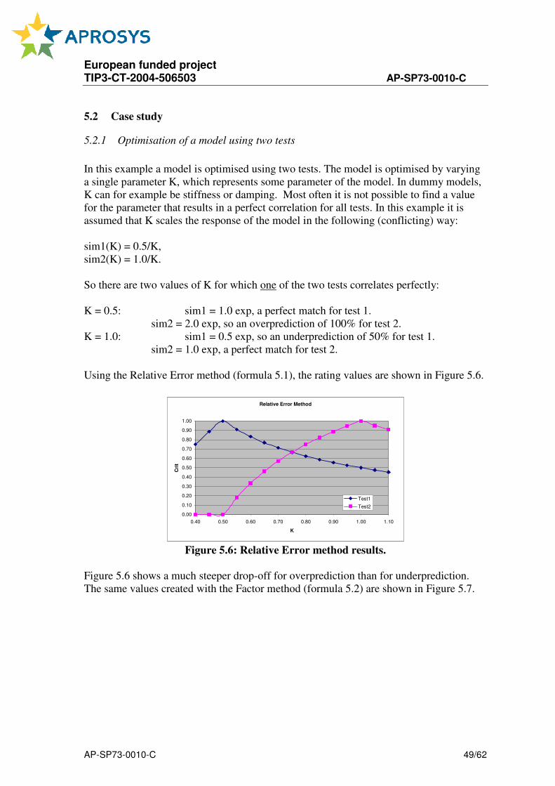
European funded project TIP3-CT-2004-506503 AP-SP73-0010-C
AP-SP73-0010-C 49/62
5.2 Case study
5.2.1 Optimisation of a model using two tests
In this example a model is optimised using two tests. The model is optimised by varying
a single parameter K, which represents some parameter of the model. In dummy models,
K can for example be stiffness or damping. Most often it is not possible to find a value
for the parameter that results in a perfect correlation for all tests. In this example it is
assumed that K scales the response of the model in the following (conflicting) way:
sim1(K) = 0.5/K,
sim2(K) = 1.0/K.
So there are two values of K for which one of the two tests correlates perfectly:
K = 0.5: sim1 = 1.0 exp, a perfect match for test 1.
sim2 = 2.0 exp, so an overprediction of 100% for test 2.
K = 1.0: sim1 = 0.5 exp, so an underprediction of 50% for test 1.
sim2 = 1.0 exp, a perfect match for test 2.
Using the Relative Error method (formula 5.1), the rating values are shown in Figure 5.6.
Relative Error Method
0.00
0.10
0.20
0.30
0.40
0.50
0.60
0.70
0.80
0.90
1.00
0.40 0.50 0.60 0.70 0.80 0.90 1.00 1.10
K
Cri
t
Test1
Test2
Figure 5.6: Relative Error method results.
Figure 5.6 shows a much steeper drop-off for overprediction than for underprediction.
The same values created with the Factor method (formula 5.2) are shown in Figure 5.7.

European funded project TIP3-CT-2004-506503 AP-SP73-0010-C
AP-SP73-0010-C 50/62
Factor method
0.00
0.10
0.20
0.30
0.40
0.50
0.60
0.70
0.80
0.90
1.00
0.40 0.50 0.60 0.70 0.80 0.90 1.00 1.10
K
Cri
t
Test1
Test2
Figure 5.7: Factor method results.
Here the drop-off for under- and overprediction is about equal within a certain range from
the peak value. The two scores of the tests can be combined using the Simple Addition
Method (formula 5.4), and RMS Addition Method (formula 5.5). The results for the
Simple Addition Method are shown in Figure 5.8.
Simple Addition
0.00
0.10
0.20
0.30
0.40
0.50
0.60
0.70
0.80
0.90
1.00
0.40 0.50 0.60 0.70 0.80 0.90 1.00 1.10
K
av
era
ge
Relative Error criterion
Factor criterion
Figure 5.8: SAM using Relative Error and Factor Method.
For the Relative Error Method Figure 5.8 shows a maximum average score of 0.75 at K =
1.0. For this value of K the performance for test 2 is optimal, but the result of test 1 is
underpredicted by 50%. The fact that the optimum value gives a perfect match for one
test, and a poor for another is because the Simple Addition Method uses linear terms in
its calculation, and the REM drop-off is not symmetric for under- and overprediction. In
this example, the optimum is found at that test that requires the highest value of K. Other
tests will be underpredicted. Using the Factor Method two maximum values are found,
one for K = 0.5 and one for K = 1.0. Two maxima are found because the Factor Method
is symmetric for over- and underprediction.
Whichever method is used to calculate the single rating scores, using the Simple Addition
Method results in a optimum that has a high score for one test and a poor score for the
other test. However, in model optimization, a solution is sought that finds a balance
between the two tests, i.e. that the results of both tests are as close as possible to the
required values.
The results for addition with the RMS method are shown in Figure 5.9.

European funded project TIP3-CT-2004-506503 AP-SP73-0010-C
AP-SP73-0010-C 51/62
RMS Addition
0.00
0.10
0.20
0.30
0.40
0.50
0.60
0.70
0.80
0.90
1.00
0.40 0.50 0.60 0.70 0.80 0.90 1.00 1.10
Relative Error criterion
Factor criterion
Figure 5.9: RMS using Relative Error and Factor Method
Because the RMS addition does not use linear terms in its calculations, none of the tests
in this example can dominate the calculation of the optimum value. For both the Relative
Error Method and the Factor Method, the optimal value for K lies between 0.5 and 1.0. If
used with the Factor Method ( = Wifac), the optimum value is K = 0.707. If used with the
Relative Error Method, the optimum value is much closer to K = 1.0, because the
Relative Error Method is in favor of underprediction.
5.2.2 Results for more complex situations
The previous example showed that for a model with two tests and one model parameter
that scales the test results, the Factor Method combined with RMS Addition gives much
better results than the combination of the Relative Error Method and Simple Addition.
However, the question is if this is still the case for a model with more parameters and
more tests.
In this section the results are shown for a model with a single parameter K and 6 tests.
The optimal values for K are chosen as 0.5, 0.6, 0.7, 0.8, 0.9 and 1.0. Only the Factor
Method criterion has been used during this evaluation.
6 tests
0
0.1
0.2
0.3
0.4
0.5
0.6
0.7
0.8
0.9
0.4 0.5 0.6 0.7 0.8 0.9 1 1.1
K
Av
era
ge
Simple addition
RMS addition
Figure 5.10: SAM and RMS for 6 tests with equal weight factors.
For this case the Simple Addition curve is much more fluent than in the case for two
tests. However there are still peaks at every test. The optimum value for the Simple
Addition is 0.8, which is exactly at one of the tests (K=0.8). Another peak is at 0.7, but its

European funded project TIP3-CT-2004-506503 AP-SP73-0010-C
AP-SP73-0010-C 52/62
value is slightly lower. The reason that these values are not equal is that the distribution
of the optimal K values between 0.5 and 1.0 was chosen linear, not harmonic.
If one of the tests has a weighting factor such that it counts more in the addition than the
other tests, the results for the Simple Addition Method are not optimal, as is shown in
Figure 5.11.
3 tests, weighted
0
0.1
0.2
0.3
0.4
0.5
0.6
0.7
0.8
0.9
0.4 0.5 0.6 0.7 0.8 0.9 1 1.1
K
Avera
ge
Simple addition
RMS addition
Figure 5.11: SAM and RMS for 6 tests with unequal weight factors.
In this example there are 3 tests with optimal K at 0.5, 0.7 and 1.0. The test with optimum
at K = 1.0 weighs just as much as the other two tests together. The optimum with the
Simple Addition Method is at K = 1.0, which more or less ignores the other tests. The
RMS Addition has its optimum around K = 0.78, which is between the optimal K values
for the tests. From this more complicated example it is concluded that the Simple
Addition Method can result in sub-optimal solutions. MADYMO therefore uses the RMS
Addition. However, it should be noted that the RMS Addition leads to a lower score than
the Simple Addition. The exact difference depends on the case, so it can not be
compensated for using a scaling factor.
5.3 Investigate the relation between rating values for signals and Injury Criteria
Objective rating of the accuracy of predicted injury criteria is essential and
interpretation is straightforward. Rating of signals is very important in building &
validating component and full system models. However the interpretation is not
necessarily straightforward. For instance, a Hybrid III pelvis acceleration rating of 0.50
may be adequate since no injury criteria directly depend on it.
In the DIP3 period we will investigate the relation between rating values for signals and
rating values for injury criteria. Here we will also consider different signal rating methods
and filtering approaches.
The final objective will be to define requirements for the accuracy of signals to obtain a
certain rating level for injury criteria.
We can investigate this in two ways:
- Analysis of an existing full dummy validation database with realistic applications.

European funded project TIP3-CT-2004-506503 AP-SP73-0010-C
AP-SP73-0010-C 53/62
- Analysis of well validated cases + variations on these cases where parameters are
changed to lower the correlation.
On either kind of database statistical analysis can be performed using regression and
RSM.
Remark on Noise Reduction:
In the rating method used, phenomena as noise and spikes in the signals still have a
negative and unwanted influence on the outcome. In particular peak values will be
affected by noise. The rating algorithm should be advanced to take into account such
disturbing effects automatically. When applying the standard SAE filters often a
significant noise level remains. The noise level is generally larger in the experimental
signal as compared to the simulation but in FE models the noise may be high also.
Different noise levels in 2 signals being compared will lead to systematic differences.
Noise can have a major effect on the rating in particular for peak values but also for
shape based criteria. For instance peak amplitude will be typically overestimated in the
signal having a higher noise level.
Our impression is that stronger low pass filtering will generally be justified to obtain a
fair rating.
There are two different problems here: the first is the problem with noisy data, in which
noise is present during one or more intervals of some significant duration. The only
solution to this problem is to low-pass filter the entire signal. The trick is of course to
determine how much filtering needs to be applied. Signal analysis using FFT is possible,
but this is quite CPU intensive and will make the rating procedure for very large data sets
a very lengthy process.
Signals that are not noisy but suffer from peaks and glitches may be low-pass filtered to
identify the peaks/glitches, which are then removed from the original by attenuation of
the signal at the point in time at which the peaks occurs. Again, the problem is to
determine which filter to use. Simply using a CFC60 filter to remove all peaks and noise
from a head acceleration signal is not a good solution because it will identify almost
everything as noise. A CFC600 or CFC180 filter may be sufficient.

European funded project TIP3-CT-2004-506503 AP-SP73-0010-C
AP-SP73-0010-C 54/62
6 LS-DYNA reading for ADVISER
6.1 Introduction
Partners need to read LS-DYNA in ADVISER to perform evaluations and stochastic
analysis. So, an extension has been develop to allow for direct reading of LS-DYNA
outputs in ADVISER sfotware.
This section demonstrates a methodology for converting LS-DYNA output into the
ADVISER program. An example has been used of a frontal impact barrier model to show
the methodology.
To complete and implement the conversion tool within the ADVISER software package a
program
has been written to convert the data from LS-DYNA output to the ADVISER output
format.
6.2 Glossary of Terms
The following terms are used within this report and are listed here to aid the reader.
6.2.1 Post-Processing Tools
T-HIS Time HIStory – A software package developed and licensed by Ove Arup to post
process data from a LS-DYNA finite element simulation.
ADVISER – A software package developed and licensed by Mecalog and freely available
for APROSYS partners.
6.2.2 Commercial Finite Element Software Packages
LS-DYNA – Livermore Software Dynamic
RADIOSS - ALTAIR
MADYMO - TASS
6.2.3 Formats of Outputs
CSV – Comma Separated Variable
ASCII – American Standard Code for Information Interchange
Binary – Binary file
6.2.4 Additional Files
To accompany this report a number of files with typical output formats have been
produced and are available from the author.
6.3 Defined Output from LS-DYNA

European funded project TIP3-CT-2004-506503 AP-SP73-0010-C
AP-SP73-0010-C 55/62
The output from a typical FE simulation in LS-DYNA can be produced in two formats,
ASCII and binary. A flow chart of this process is shown in Figure 6.1. For detailed FE
models there will be a large amount of data generated and therefore the binary data may
be a preferred option as it has the capability to store more data in a compressed format.
ASCII data has the advantage of being able to be read by a wide range of software
packages whereas the binary data will be only be able to be imported into a few
purposefully designed packages. There also a few instances when the specific output data
is only available in certain formats, which will then dictate the option chosen by the
analyst. However the vast majority of data is available in both formats.
6.3.1 ASCII data
The ASCII formatted data can be processed by two methods - option 1 and 2. the format
for the ASCII data is shown in Figure 6.2. There have been two nodes selected for output,
nodes 40802 and 177482. These are shown in the left hand column (lines 4,5,8 and 9).
Reading from left to right there are a number of data points which refer to the respective
nodes and the headings supplied in line 3 explain their definition. Lines 8 and 9 are a
continuation of lines 4 and 5.
The nodal accelerations, velocities and displacements can be read directly from this file
for any particular node at any particular time. The block of data shown in Figure 6.2 is
repeated for the next specified time state, which is shown in line 2. The LS-DYNA user
has the capability to specify the number of time states that are recorded for the
simulation. For the example with the barrier output, a time interval of 1e-4 sec was
specified.
The data shown in Figure 6.2 is written to a file called NODOUT after the completion of
a LS-DYNA simulation. There are other data time histories which can be gleamed from
other files and these are detailed in the T-HIS manual.
From Figure 6.1, Option 1 describes a process of reading this format of data and
converting it into a format suitable for ADVISER. To aid this conversion process an
example of the output format can be supplied.
Option 2 describes a different approach of using the T-HIS software package which will
be able to convert the ASCII formatted output into a CSV type of data output. This can
then be subsequently imported into ADVISER. This method involves another step in the
conversion process and the capability to have access to the T-HIS software and is
therefore not recommended.
There is a software package commercially available [OAS01] which will automatically
run immediately after a LS-DYNA simulation has finished and generate files in a CSV
format which can be read into ADVISER. This use of Reporter has been shown as
Option 3 in Figure 6.1.

European funded project TIP3-CT-2004-506503 AP-SP73-0010-C
AP-SP73-0010-C 56/62
Figure 6.1: Flow Diagram of Conversion from LS-DYNA output to ADVISER
LS-DYNA
Simulation of
Frontal Barrier
Model
ASCII
data Binary data
Read into
ADVISER
Import to
THIS
and
convert
to CSV
file
format.
Convert
Binary
data
directly
into
Read
directly into
ADVISER
with
Conversion
Tool
Read into
ADVISE
R
Option 1 Option 2 Option 3 Option 4
Import to
THIS
and
convert
to CSV
file
format.

European funded project TIP3-CT-2004-506503 AP-SP73-0010-C
AP-SP73-0010-C 57/62
1. BAR IMPACT- FINE MESH WITH TOPPLATE 0.2 SHEAR AND 0.2 TENSILE
i. ls-dyna ls970s.6763.169 date 11/28/2005
2. n o d a l p r i n t o u t f o r t i m e s t e p 1 ( at time 0.00000E+00 )
3. nodal point x-disp y-disp z-disp x-vel y-vel z-vel x-accl y-accl z-accl x-coor y-coor z-coor
4. 40802 0.0000E+00 0.0000E+00 0.0000E+00 0.0000E+00 -1.0000E+04 0.0000E+00 0.0000E+00 0.0000E+00 0.0000E+00 1.6925E+02 2.0000E+00 4.4575E+02
5. 177482 0.0000E+00 0.0000E+00 0.0000E+00 1.0000E+04 0.0000E+00 0.0000E+00 0.0000E+00 0.0000E+00 0.0000E+00 9.2500E+00 4.2000E+01 4.8575E+02
6. n o d a l p r i n t o u t f o r t i m e s t e p 1 ( at time 0.00000E+00 )
7. nodal point x-rot y-rot z-rot x-rot vel y-rot vel z-rot vel x-rot acc y-rot acc z-rot acc
8. 40802 0.0000E+00 0.0000E+00 0.0000E+00 0.0000E+00 0.0000E+00 0.0000E+00 0.0000E+00 0.0000E+00 0.0000E+00
9. 177482 0.0000E+00 0.0000E+00 0.0000E+00 0.0000E+00 0.0000E+00 0.0000E+00 0.0000E+00 0.0000E+00 0.0000E+00
Figure 6.2. ASCII format of LS-DYNA Output

AP-SP73-0010-C 58/62
6.3.2 Binary Data
The binary formatted output can also be processed by two methods - option 3 and 4. In a
similar manner to option 2, the binary data can also be processed by T-HIS and Reporter and
delivered in a CSV format. This process has been shown as Option 3 and an example of CSV
formatted output is shown in Figure 6.3.
0 0
9.90E-05 0.010905
0.00019998 0.67154
0.00029898 0.990801
0.00039996 1.22673
0.00049896 1.53442
0.00059994 2.03845
0.00069894 2.54804
0.00079992 1.98976
0.00089892 1.78006
0.0009999 1.51683
0.0010989 1.61363
0.00119988 1.56959
0.00129888 1.12019
0.00139986 1.08225
0.00149886 0.915008
0.00159984 0.659422
………………… ……………
………………… ……………
↓↓↓↓↓↓↓↓↓ ↓↓↓↓↓↓
Figure 6.3: CSV formatted Output
The binary output obtained from an LS-DYNA simulation is used by packages such as THIS
and converted into graphical plots of data as shown in Figure 6.4. An attempt was made to
convert the binary output to a format suitable to read directly into ADVISER. In the event,
this operation was difficult to perform as it involved deciphering a complex binary notation.
The ASCII format of LS-DYNA was a more logical and less complex type of data for the
conversion process. This conversion of binary data has been shown as Option 4 in Figure 6.2

AP-SP73-0010-C 59/62
Figure 6.4: T-HIS Graphical Output for Nodes 40802/177482
6.4 Implementation into ADVISER
To implement the conversion of LS-DYNA results into ADVISER a program will be
necessary to read the format as shown in Figure 6.2. The selection method of which nodes to
use in the analysis part of ADVISER, will be similar to what is currently available for other
software packages, such as RADIOSS and MADYMO. The aim of the conversion tool is to
reproduce graphs similar to the nodal results as shown in Figure 6.5. The graph shown has
been generated by using Option 2, but is reliant on using the T-HIS software package. With
the conversion tool the output from such a package will be able to be read directly from LS-
DYNA using Option 1.

AP-SP73-0010-C 60/62
Figure 6.5: ADVISER Graphical Output for Nodes 40802/177482
6.5 The LS-DYNA Output Converter
An executable has been created to read the ASCII data from a typical LS-DYNA output and
convert the files to a format which can be read into ADVISER.
The executable is entitled ‘LS-DYNA Convert’
When the executable runs the program searches for the ‘nodout’ file in the same directory as
the executable. The output from the program is then delivered to the same directory. Each
node is identified by its number followed by an extension which indicates its data component.
The following data components are obtained from the program:
‘node number’.xac x acceleration
‘node number’.yac y acceleration
‘node number’.zac z acceleration
‘node number’.xvel x velocity
‘node number’.yvel y velocity
‘node number’.zvel z velocity
‘node number’.xdis x displacement
‘node number’.ydis y displacement
‘node number’.zdis z displacement
6.6 Conclusions
1. Various options of translating output files from LS-DYNA into an ADVISER format
have been investigated and demonstrated.
2. It has been shown that the Option 1 method of translating LS-DYNA results into
ADVISER is the most efficient and practical method.
3. Option 1 will be most adaptable to a wide range of analysts, as there is not a pre-
requisite for additional interface software.
4. An additional interface software code has been written to allow nodal data to be
incorporated into ADVISER to allow the translation process to be complete.

AP-SP73-0010-C 61/62
7 REFERENCES
[BEU92] Beucher S., Meyer F., The morphological approach to segmentation : the
watershed transformation, In E. Dougherty, editor, Mathematical Morphology in Image
Processing, Marcel Dekker, New-York, 1992.
[CAN83] J.F. Canny, Finding edges and lines in images, Technical report AI-TR-720,
MIT Artificial Intelligence Laboratory, Cambridge, Massachussets, USA, 1983
[CAN86] J.F. Canny, A computational approach to edge detection, IEEE Trans. Pattern
Analysis and Machine Intelligence, 8(6):768-769, November 1986
[CHAN98] Chan S. L., Purisima E. O., A new tetrahedral tessellation scheme for
isosurface generation, Computer and Graphics, 1998, 22(1), 83-90.
[JAS02] Jasjit S. Suri, S. Kamaledin Setarehdan, Sameer Singh, Kamaledin
Setarehdan, "Advanced Algorithmic Approaches to Medical Image Segmentation: State Of
The Art Applications in Cardiology, Neurology, Mammography and Pathology", Springer
Verlag February, 2002 Hardcover, ISBN: 1852333898
[LUC01] L. Lucchese and S. Mitra., “Color image segmentation: A state-of-the-art
survey.”, Proc. of the Indian National Science Academy (INSA-A), 67(2):207--221, 2001.
[RAD05] Radke RJ, Andra S, Al-Kofahi O, Roysam B., ”Image change detection
algorithms: a systematic survey”, IEEE Trans Image Process. 2005 Mar;14(3):294-307.
[ROE99] J. B. T. M. Roerdink and A. Meijster, "The Watershed Transform: Definitions,
Algorithms and Parallelization Techniques," Institute for Mathematics and Computer Science,
University of Groningen, Groningen, The Netherlands, IWI 99--9-06, 1999.
[SAH88] Sahoo, P. K., Soltani, S., Wong, A. K. C. and Chen, Y. C., A Survey of
Thresholding Techniques, Computer Vision, Graphics and Image Processing, Vol. 41, 1988,
pp. 233-260
[ZHA01] D. Zhang, G. Lu, "Segmentation of Moving Objects in Image Sequence: A
Review," Circuits, Systems and Signal Processing, Vol. 20(2) , 143-183, 2001.
[ISO97] ISO Technical Report 9790 (1997) Road vehicles – Anthropomorphic side
impact dummy- lateral impact response requirements to assess the biofidelity of the dummy,
ISO/TC22/SC12/WG5 (Anthropometric Test Devices), Document N455 – Revision 4 (May
1997).
[DAL05] Dalenoort, A., Griotto, G., Mooi, H., Baldauf, H., Weissenbach, G. (2005). A
Stochastic Virtual Testing Approach in Vehicle Passive Safety Design: Effect of Scatter on
Injury Response, SAE 2005 World Congress and Exhibition, paper number 2005-01-1763,
April 2005.
[DEL05] Delannoy P., Martin T., Castaing P., Comparative evaluation of frontal offset
tests to control self and partner protection, ESV Paper 05-0010.

AP-SP73-0010-C 62/62
[HOV05] Hovenga P.E., Spit H.H., Uijldert M. , Dalenoort A.M. (2005), Improved
prediction of Hybrid-III injury values using advanced multibody techniques and objective
rating. SAE World Conference 2005, paper SAE 2005-01-1307.
[HOOF03] Hoof J van, Puppini R., Baldauf H., Oakley C., Kayvantash K. (2003).
Adviser: A Software Tool for Evaluation and Rating of Numerical Models in Crash Safety
Analyses, ESV Conference 2003, Paper Number 483.
[HOOF03b] Hoof J. van., Lange R. de, Wismans J.S.H.M. (2003). Improving Pedestrian
Safety Using Numerical Human Models. Stapp Car Crash Journal, Vol. 47 (October 2003).
[LAN05] Lange Ronald de, Rooij Lex van, Mooi Herman, Wismans Jac (2005).
Objective Biofidelity Rating of a Numerical Human Occupant Model in Frontal to Lateral
Impact. Stapp Car Crash Journal, Vol. 49 (November 2005), pp. 457-479.
[MEI04] Meijer R., Rooij L. van (2004), HUMAN MODEL VALIDATION
PROCEDURES VITES Deliverable D1-8 and D1-9, VITES document 14/040112/TB
[RHU02] Rhule, H.H., Maltese, M.R., Donelly, B.R., Eppinger, R.H. (2002)
Development of a new biofidelity ranking system for anthropometric test devices, Stapp Car
Crash Journal, Vol. 46, pp. 477-512, Paper no. 2002-22-0024.
[PUP01] Puppini R., Hoof J. van (2001) General Validation Procedure for Numerical
Models used in Automotive Safety Simulations. VITES Deliverable D1-4, 1/011213/D/A,
VITES-GenValProc, Issuing date, A 2001-12-12.
[UTA04] UTAC, April 2004, Self and partner protection test and assessment protocol
based on current regulation r94 and PDB barrier.
[VIT03] VITES Reports on correlation criteria
[OAS01] REPORTER, Oasys LSDYNA environment software, version 9.2, Ove Arup.