evaluating circuit emulation adapters

EEvvaalluuaattiinngg CCiirrccuuiitt EEmmuullaattiioonn AAddaapptteerrss

TTIIKK--RReeppoorrtt 225544

Rainer Baumann, [email protected] Dr. Ulrich Fiedler, [email protected]

6th July 2006

Abstract In metropolitan areas the deployment of optical fiber and Gigabit Ethernets leads to an expansion of packet-switched networks with large available capacities. These capacities could thus be employed to carry traffic from existing GSM/UMTS base stations and PBX (Private Branch Exchanges). Carrying this traffic requires an emulation of E1/T1 telephone circuits over Ethernets, i.e. E1/T1 PDH/SDH signals from base stations need to be packetized and encapsulated in a circuit emulation adapter (CEA) before being sent over the Ethernet. The key problem with this emulation is to adjust the buffer play-out rate in the receiving CEA to the rate of the sending CEA. This synchronization is necessary: (i) to avoid long-time receiver buffer under- or overflows since base stations are up for weeks and months and (ii) to preserve the frequency of PDH signals across the Ethernet. TIK/ETH and Siemens have started the CoP (Circuit-over-Packets) project to address this problem and to build a new CEA demonstrator. This thesis documents laboratory measurements of the synchronization between pairs of CEA demonstrators over metropolitan Gigabit Ethernets, i.e. we have measured the Maximum Relative Time Interval Error (MRTIE) between the PDH signal that goes into the sending CEA and the PDH signal that comes out of the receiving CEA. To make measurements reproducible, we have employed the network emulator RplTrc [2] to emulate traffic patterns of a Gigabit Ethernets. RplTrc has also been developed by TIK/ETH. To get a feel for the achievements of the CoP project, we have additionally compared measurements of the CoP's CEA to measurements with three commercially available CEAs ("product A, B, C"). From our measurements, we conclude that the CoP's CEA generally outperforms the CEA C. The CoP's CEA also shows better performance in long-term synchronization stability than the CEA B. However, the synchronization algorithm of the CEA B is more robust to variable network conditions. Finally, we have found that the CEA A shows higher quality level for short-term synchronization stability than the CoP's CEA, while long-term behaviors are comparable. The CEA A is slightly more robust to different traffic scenarios, but equally sensitive to the limited delay (im)precision of RplTrc. We explain this slightly better performance of the CEA A with the arithmetic limitations of the Siemens board used to implement the CoP's CEA demonstrator.

Contents Contents .................................................................................................................3 1. Introduction......................................................................................................4

1.1 Circuit Emulation Services over Packets – Backgrounds and Basic Properties.......5 1.2 Circuit over Packets Project..........................................................................6

2. Backgrounds and Applications ........................................................................... 10 2.1 Introduction............................................................................................. 10

2.1.1 Traditional TDM Networks ....................................................................................10 2.1.2 SDH/SONET Networks ..........................................................................................12 2.1.3 Disadvantages of TDM ..........................................................................................12 2.1.4 Evolution of Packet networks ...............................................................................13 2.1.5 Going to Packet Networks ....................................................................................13 2.1.6 Circuit emulation Services....................................................................................14 2.1.7 Conclusion..............................................................................................................21

3. Evaluation Methodology.................................................................................... 22 3.1 Measurement setup .................................................................................. 22

3.1.1 PDH Signal .............................................................................................................23 3.1.2 Investigated Network Conditions.........................................................................23 a) Normal Mode .........................................................................................................23 b) Extreme mode .......................................................................................................24 c) Artificial Scenarios.................................................................................................24

3.2 Metrics for Performance Evaluation ............................................................. 26 3.2.1 Metrics for Jitter UI (Unit Intervals) ....................................................................26 3.2.2 Metrics for Wander................................................................................................26 a) Time Interval Error (TIE)......................................................................................27 b) Maximum Time Interval Error (MTIE) .................................................................27 c) Time Deviation (TDEV) .........................................................................................27

4. Evaluation Results ........................................................................................... 29 4.1 CoP Demonstrator Measurement Results...................................................... 29

4.1.1 Test time and procedure ......................................................................................29 4.1.2 Measurement results ............................................................................................30 d) Normal Mode .........................................................................................................30 e) Extreme Mode .......................................................................................................36 f) Disconnections.......................................................................................................37 g) Spanning Tree Rebuilding.....................................................................................39 h) Heavy Bursts .........................................................................................................40 i) Losses ....................................................................................................................41

4.2 Performances of competitors CEAs .............................................................. 42 4.2.1 CEA of the Competitor A.......................................................................................42 4.2.2 CEA of the Competitor B.......................................................................................47 4.2.3 CEA of the Competitor C.......................................................................................51

4.3 The CoP Demonstrator against Competitors CEAs.......................................... 51 5. Conclusion...................................................................................................... 52 Annexes................................................................................................................ 53 ANNEX A REQUIREMENTS FOR INPUT FREQUENCY TOLERANCE............................ 54 ANNEX B REQUIREMENTS FOR JITTER AND WANDER.......................................... 54

B.1 Jitter and wander tolerances.............................................................. 54 B.2 TDM jitter generation........................................................................ 56 ANNEX C-TRACES ........................................................................................... 60 ANNEX D- TEST PLAN...................................................................................... 66

Bibliography .......................................................................................................... 68

Evaluation of COP /68

1. Introduction

Data traffic on the world's telecommunication scene is now much more widespread than the voice traffic. Almost all predictions state that the tendency of replacing voice with data services is still rising very fast.

It is also evident that majority of profit is still generated by the voice traffic. However, data-centric networks which present a great part of today networks have quite different infrastructure and technology requirements than that designed to carry voice samples. Packet networks have been designed specifically for use with data services. The variable nature of data traffic flow, coupled with the time insensitivity, have required designers to develop networks with characteristics well suited to managing these features. Today’s packet networks have significant advantages over the circuit-switched PSTN (Public Switched Telephone Network), namely their scalability, cost efficiency relative to bandwidth, large available capacity and simplicity. Even though, this equipment must be capable to deliver voice services equal in quality to the current best solution i.e. to the PSTN.

Big potential of the newly developed packet based networks has also been seen by many service providers’ customers. Within the Enterprise, these customers are moving very fast towards an all packet future; however they still demand high levels of quality of service (QoS) for voice services. To achieve carrier-grade QoS, service providers may choose to route Enterprise Voice over Packet (VoP) traffic over the PSTN. This requires converting VoP traffic back into TDM (Time Division Multiplexing), thus gaining access to PSTN’s quality features, while maintaining data traffic within the packet network (see Figure 1.1)

Figure 1.1: Two ways of VoP Traffic Routing:

1. back over PSTN, 2. over low latency Packet Network

Conversely, with a low latency Packet Network, delivering high levels of QoS, service providers may choose to route all voice traffic over the Packet Network via a Media Gateway and Softswitch.

Access technologies are also various, ranging from DSL (Digital Subscriber Line) to cable, T1/E1 to POTS (Plain Old Telephone Service) and the widely deployed Dial-up. All these technologies are adding to the increase in data traffic. Fiber is also pushing closer to the edge, providing for aggregation of ever increasing data traffic. Fiber deployment encourages the increase of packet networks and the proliferation of Gigabit Ethernet, although Ethernet is not exclusively wedded to fiber.

The interesting questions are now coming: Should a service provider choose to implement a packet network at the edge? How would it interface already installed technologies, such as TDM, ATM (Asynchronous Transfer Mode) and even Ethernet? The new solution must be cost effective, at the same time providing levels of service for which customers will pay. Here the choice of architecture is crucial and is the place where the Circuit Emulation over Packets (CoP) technology wins through.


1.1 Circuit Emulation Services over Packets – Backgrounds and Basic Properties

The growth of data information has been much heralded over the last few years. The logical conclusion is that the world is going to go IP (Internet Protocol). Since data is playing the dominant traffic role, the world's telecommunications networks should be of a type best suited for carrying data, easing the engineering problems and operational expenditure associated with running the networks.

One of the challenges for carriers in changing their networks is how to connect old customers with already existing TDM-based equipment to a completely new network. VoIP (Voice over Internet Protocol) seems to be one way to handle this, but not the only one. Furthermore, it is not a complete solution, since not all TDM connections are voice based. Most companies' data networks are currently connected via TDM connections, e.g. T1 or E1.

The revolutionary approach is to convert the traffic right at the edge of the network. That means a company's data traffic would be terminated at the network edge, and then routed onto the data network. However, this is a radical change, endangering the carrier's primary revenue stream if it fails.

The evolutionary solution is found in replacing only the parts of the network which are under the biggest pressure due to volumes of traffic. Most often, this is the access network, especially in concentrated locations such as the metropolitan area. For instance, the access network could be replaced by a packet based network, such as Metropolitan Ethernet, or Resilient Packet Ring (RPR).

The main point underlying this great idea is the fact that it is not necessarily required to replace the entire existing equipment base. On one side this enables the customers to maintain their existing infrastructure, and on the other the carriers to evolve their network gradually, replacing only the parts that need replacing. Hence it reduces the risk to the existing revenue stream that the revolutionary, disruptive replacement model could represent.

Term Circuit Emulation (“to perform the same behavior as circuit does”) has its origin in the ATM world, for much the same reason: at that time carriers were trying to upgrade their TDM networks to ATM, but with necessity to maintain support of customers already using TDM-based equipment. Therefore the ATM Forum defined a way to "emulate" a TDM circuit across an ATM network, such that at the network ends it appeared as though the circuit was being transmitted across a conventional TDM network.

This approach has been taken up in the packet switched world by several bodies, including the IETF (Internet Engineering Task Force), the Metro Ethernet Forum and the MPLS (Multiprotocol Label Switching) Forum. The essential concept is to emulate a circuit-switched service on top of a packet-switched network (see Figure 1.2 CESoP stands for Circuit Emulation Services over Packets)

Figure 1.2: Circuit Emulation Services over Packets-

A tool to emulate a circuit-switched service on top of a packet-switched network


Some of the basic properties and challenges of Circuit Emulation Services over Ethernet networks are:

• Granularity: Instead of switching at the individual channel level, CESoP switches at the circuit level, where the circuit can be T1/E1, T3/E3 or even OC3/STM-1 or higher. This gives rise to efficiencies in terms of network management and control.

• Low Latency and more efficient Bandwidth (cheap bandwidth due to the large capacity of fiber).

• Flexibility: Circuit emulation makes no assumptions about the type of traffic being carried across the network. The traffic could be voice, video, or packet data.

• Synchronization: This is certainly one of the main technical challenges to overcome with circuit emulation. The bits have to be played out of the packet network at the same rate as which they entered it, otherwise the buffer at the destination node will either fill up or empty. The net result would be the same: loss of data integrity. In a TDM network, the circuit itself carries the clock. With a packet network, this is no longer the case. Therefore, unless a common clock can be distributed to each end by an alternative means, some kind of clock recovery is necessary, e.g. recovering the frequency of the original clock from the arrival rate of packets at the destination node.

The main carrier application of circuit emulation comes from emerging deployment of fiber which fosters the proliferation of Metropolitan Gigabit Ethernets on the top of wavelength division multiplexing equipment. Thus a major aspect of interest is to employ these networks to connect legacy Private Branch Exchanges (PBX) and GSM (Global System for Mobile Communications)/UMTS (Universal Mobile Telecommunication System) base stations to the core telephony network. This protects investments in existing infrastructure and creates new revenues for network providers.

Figure 1.3: Circuit emulation over MAN Gigabit Ethernet: to connect base station to the core PDH network

the sending circuit emulation adapter (CEA) packetizes E1/T1 the PDH signal from the base station into

Ethernet frames; the receiving CEA reassembles the original PDH signal

1.2 Circuit over Packets Project

The CoP (Circuit over Packets) project together with this thesis heads towards both implementation and verification of such an emulator. First part of the project was dedicated to evaluation of already existing algorithms for timing synchronization, i.e. algorithms for adjusting the receiver buffer play-out rate to the sender packetizing rate, where both sender and receiver are CEA (Circuit Emulation Adapter) Units. In the second stage one completely new circuit emulation adapter is developed. The main task was to resolve the


problem of two-level synchronization: board and interface synchronization since both are very important in clock recovery mechanism.

• Synchronization issues A CEA has more than one PDH interface. These plesynchronous interfaces may run at

slightly different frequencies. In the case of TDM signals nominal frequency is 8000Hz with variation ± 50ppm. This means that signals coming at different PDH interfaces may not have the same frequency (relative difference between each two interface frequencies has to be less than δ, for δ small, positive number). However, it is desirable to reproduce the frequency of each incoming signal at the receiving CEA since the circuit emulation needs to prevent loss of information while having no means to adjust frequencies of incoming signals. Put simply, different PDH interfaces of the sending CEA could be unsynchronized but reproduced signal of the corresponding interface at the receiving CEA should have the same frequency as the original incoming one (see figure 1.4).

Figure 1.4: Two stage synchronization: 1. board level / 2. interface level

Board level synchronization stands for the problem of eliciting Master and Slave units since all units have to be synchronized to one common clock source in order to avoid packet losses. If several CEAs should be interconnected algorithm has to determine which board will play Master role to which all other units should synchronize their clocks. This leads to spanning-tree like relations as depicted in figure 1.5. In the case of CoP demonstration adapter this problem is addressed by manually assigning priorities.

Figure 1.5: Logic spanning tree for board clock rate synchronization

• Evaluation setup Evaluation of CEAs looks as following (see the Figure 1.6):

PDH signal is given externally to the sending CEA as the input signal. At the sender's

side, a CEA packetizes and encapsulates TDM signals and sends them over packet-switched network emulated by the NistNet. NistNet is a tool capable to reproduce dynamics of real


networks in order to test the performance of network sensitive applications, devices, and protocols. Due to the ability to replay large packet traces, the tool is capable to account for traffic characteristics such as long-range dependence which are key in performance evaluations. At the receiver's side, a CEA de-encapsulates and de-packetizes the incoming packets. Depending on the algorithm for adjusting the receiver buffer play-out rate to the sender packetizing rate, recovered E1 signal would have to have the same frequency as the original signal. This play-out buffer is necessary since frame delays on an Ethernet are highly variable. The output of the receiving CEA is than fed back to the PDH analyzer to evaluate the quality of clock recovery. Ethernet links were using 100 Mbps, full duplex mode.

Moreover, a CEA usually works bi-directional since the TDM signal is also bidirectional and supports emulation of multiple circuits. Albeit the quality of service problem with regards to frame loss and delay is believed to be solvable in metropolitan networks, clock rate synchronization over the Ethernet is still a remaining problem. As we have mentioned above highly accurate clock rate synchronization of sending and receiving circuit emulation adapter is necessary to prevent long-term receiver buffer over-/underrun. For VoIP these overflows are not a problem since calls only last for a few minutes. However, base stations are up for weeks and months. As consequence, requirements on clock rate synchronization between sending and receiving circuit emulation adapters are much more stringent. The adjustment may be very difficult at the presence of bursty cross traffic

Figure 1.6: Measurement setup: TDM signal from PDH generator is given to the sending CEA as an input. After encapsulation and packetization signal is sent to the receiving CEA

over packet-switched network emulated by the NistNet. Receiving CEA de-encapsulates and de-packetizes the incoming packets. Recovered TDM signal should have to have the same

frequency as the original one. Quality of clock recovery is checked by PDH analyser

• Performance metrics and delay patterns

The two most important characteristics of the signal propagating through the network are jitter and wander. They are defined respectively as “the short-term and the long-term variations of the significant instants of a digital signal from their ideal position in time”. In ITU-T G.801 standard jitter is defined as phase variation with frequency components greater than or equal to 10 Hz while wander is defined to be a phase variation at a rate less than 10 Hz. The most important thing in measuring jitter and wander is the reference clock they are compared to. By definition, a signal has no phase variation when referenced to itself.

In this project we are more interested in wander measurements especially in the two wander metrics: MTIE (Maximum Time Interval Error related to Peak-to-Peak wander) and TDEV (Time Deviation related to root mean square wander) which are defined in the Chapter 3.

To test performance of all CEAs we use different classes of delay patterns. We have generated exponentially distributed delays and also measured patterns with no special events in real networks (see the 3.1). Besides traffic without special events we have tested


the CEAs on classes that can cause difficulties for their synchronization algorithm. These potentially critical situations are: outage, heavy bursts and the spanning tree reconfiguration. We have generated outages of: 10ms, 100ms, 1s, 10s and 100s, heavy bursts as uniformly distributed delays up to 200µs, 1 ms, 10 ms and 100 ms lasting for 100s and 1000s and reconfiguration of the spanning tree with delays 0ms, 10ms, 500ms, 1s and 5s and the minimum delay change equals: -100μs, 0μs, +100μs.

• Results, conclusion and thesis structure

The thesis is structured as follows: Chapter 2 explains to readers, in more details then written above, the reasons why it was necessary to come up with the new solution in carrying TDM traffic. It presents some background approaches and also some application scenarios. As previously mentioned Chapter 3 introduces measurement setup, MTIE/TDEV measurements to determine how good the synchronization is, as well as some interesting traffic patterns which are tested in order to see whether CEAs are capable to perform the emulation under different network conditions. We have measured the performance of CEA developed in the CoP project and have compared this performance to the performance of other CEAs available on the market. Chapter 4 provides readers with the obtained results. From our measurements we conclude that the performance of the CoP demonstrator is on the very high level for all realistic scenarios including extreme network conditions and packet losses. In several tested traffic patterns results show no successful clock recovery. These behaviors are due to the well known issues: arithmetic limitations on the CoP board which can easily be solved, delay precision and limited buffer size of the NistNet which are configuration subjects. Compared to three tested competitors’ CEAs, already full products, CoP demonstrator shows almost the same or in one case significantly higher quality of clock recovery. We thus recommend to give the special attention to the fact that CEA developed in the CoP project is only a demo version which has high-grade properties and huge space for improvements in further developments. Chapter 5 ends this thesis giving an short overall conclusion of the CoP demonstrator performance.


2. Backgrounds and Applications

In traditional telecommunication networks, voice has always been carried using Time Division Multiplexing. The reason lies in very high reliability and robustness for connections, and predictable delays for voice samples, which together provides a superior quality. On the other side popular Internet Protocol (IP) networks are characterized by ubiquitous nature and significant cost advantages; attributes that has led more and more to the convergence of TDM traffic into the IP networks. Packet networks, initially developed to carry only data traffic, are now facing the challenge of carrying real time services like voice and video. Both, economical advantage of low rates data traffic and technological improvement of multiple packetized data streams using statistical multiplexing, are pushing the evolution of convergence. Some devices which bridge the TDM and IP traffic are also able to transparently handle structured or unstructured primary rate data traffic over IP networks, thus providing circuit emulation inter-working function.

This Chapter begins with evolution of TDM based networks. It faces the challenges of creating circuit emulation services over data packet networks. It also presents schematic description of an optimal architecture of the device capable to do both the packetization and re-assembly process, providing in the same time timing recovery over packet networks. Chapter ends with the most common network scenarios, as well as with provisioned future applications.

2.1 Introduction

Rapid increase in access and edge network transport is forcing service providers to consider other cost effective transport mechanisms. For a long time circuit switched networks, such as E1/T1/E3/T3 and SDH/SONET, have been the core of voice traffic. With the evolution of packet networks, there are efforts to transport voice over packet switched network. Circuit Emulation Services transport digital trunks such as E1/T1/E3/T3 as well as SDH/SONET circuits over packet networks. There are many challenges facing the realization of those virtual circuits; how to provide interfaces which give the same performance characteristics as the circuit switched networks is certainly one of the most important tasks.

2.1.1 Traditional TDM Networks

The digital transport networks were gradually developed from isolated links connecting analog switching systems for Analog Public Switched Telephone Networks (PSTN). Digitized voice channels were multiplexed to form serial streams and then transported over twisted pairs or coaxial cables; after performing framing and line coding. At the receiver end, the clocks were extracted from the line, data clocked on to receive buffers and afterwards de-framed in order to get the voice channels. Since the digital interfaces were transparent to networks, there was no special requirement to relate the internal clock rates of different systems. The same fact stands for the original higher multiplexing techniques: they allowed all digital signals in the network to operate with completely unsynchronized clocks.


Figure 2.1: PDH receiver interfaces

The term Plesiochronous originally means “near synchronous”. In other words, PDH signals are allowed to have frequencies varying from the nominal one, but only inside the given interval of tolerance. In the primary rates this difference is taken care of by elastic stores; in higher multiplexing rates by bit stuffing.

Predominantly there are three standards for digital trunks of primary rates: the E1 interfaces, popular in Asia and Europe, the T1 interfaces in North America and the J1 interfaces in Japan. T1 and J1 are identical except for the alarm signals and the error correction mechanism. T1 and E1 differ in framing techniques, number of digital voice channels multiplexed as well as in line coding. In PDH transmission chain, a number of lower level digital signals are bit-wise time division multiplexed together to form a higher level signal, and the bit rate of the higher level signal is greater than the sum of the rates of the forming signals. There are various overhead functions in the higher rate signal, such as framing patterns to allow identification of the individual signals, parity or other error detection bits, various types of communication channels for alarms and maintenance etc. Table 2.1 shows the hierarchy of signals.

Table 2.1: Digital Hierarchies

The bits of each lower level digital signal are written into an input buffer (one buffer per input signal), with the frequency equal to the incoming signal instantaneous bit rate. The forming bits are then read, according to the local system clock, and multiplexed by bit-interleaving. In order to adjust close deviations in the frequencies among different forming signal and the overall multiplexed signal, certain bit positions within the output frame (justification or stuffing opportunity bits) can carry either signal or dummy bits. In most standard frame formats, one justification opportunity position is reserved for each signal in each multiplex frame. Decision, if the stuffing opportunity bit should carry information or be a dummy, is made frame by frame on the basis of a buffer threshold mechanism. Therefore, the actual number of useful bits in the output multiplex frame varies dynamically and the transmission capacity gets adapted to the actual bit rate of the incoming signals.


Figure 2.2:Plesiochronous Digital Hierarchy

2.1.2 SDH/SONET Networks

PDH networks are working using independent clocking mechanisms. The small differences in clock rates eventually results in buffer slips. The effects of buffer slips in voice conversations are negligible and cause no real performance degradation to voice transport within the specified slip limits. But if the networks are assumed to carry traffic other that voice, like data or video, those slips are no longer affordable. The buffer slips starts to cause serious performance degradations. To avoid this effect new synchronous network architecture was proposed. The basic property is synchronization of all network elements which in this case all are running on the same average frequency. The transient variations were taken care by a mechanism called pointer adjustments. The Asian and European standard for the synchronous network is called SDH and the North American standard is called SONET.

SONET/SDH technology has been accepted as a proven standard for transport networks. Traditionally, the backbone networks for high speed transport are built on SONET/SDH technology, due to its inherent nature of robustness and performance advantages. For example self-healing bi-directional ring architectures offered superior availability with error performance monitoring capabilities, enough provisions for network management and rapid provisioning of services with “Add-Drop” architecture.

Table 2.2: SDH and SONET

2.1.3 Disadvantages of TDM

For a long time, circuit-switched networks have been the principal medium for the information transfer. They dedicate a circuit with a fixed amount of bandwidth for the whole duration of connection, regardless of a user's actual bandwidth usage. The recent growth in data traffic, particularly the growth in the number of Internet users, has placed significant strains on the capacity of traditional circuit-switched networks. This is due to the fact that these networks were initially deployed to handle only voice communications. They are not able to handle data efficiently and can not scale cost-effectively to accommodate the growth in volume of data traffic. Moreover, circuit-switched networks were built based on complex technologies which have historically limited the entrance of new competitors and have made the development and introduction of new services to be very difficult.

The main disadvantage of SONET/SDH networks lies in their optimality specifically for TDM traffic. The protocol lacks functions required to effectively manage traffic other than traditional voice traffic based on TDM technology. Most of the high speed transport backbones are based on SDH/SONET ring architecture. In a SONET/SDH ring, there are limitations on the number of nodes that can be placed over. There is another category of SONET/SDH terminal equipment, which is used in point to point applications. In order to increase bandwidth in point to point networks the technology needs to implement multiple optical fibres; which is not so cheap solution. The robustness of SONET/SDH networks is guaranteed by protection circuits. But even though it offers an excellent recovery in minimal time, considerable bandwidth is consumed. That makes the networks inflexible; the whole ring has to run on the same rate.


2.1.4 Evolution of Packet networks

Last few years, the development and deployment of packet based networks have increased tremendously. This growth is primarily driven by the growth of internet and multimedia traffic. The main advantages of IP networks, besides obvious simplicity and lower relative costs, are their ability to handle variety of media types, resilience, and the huge amounts of bandwidth (tens of Mbps) they offer.

Packet switched networks were originally designed only for data communications and computer networking. The information is divided into the form of small packets; packets from multiple sources are then sent over a single network simultaneously, and afterwards reassembled at the destinations. Compared to circuit-switching, packet switching enables more efficient utilization of available network bandwidth, as the former mostly works on statistical multiplexing. Single node-to-node link can be dynamically shared by packets over time; it can assign priorities to packets and also enable the new connections even the traffic increases. Packet networks allow for the cost-efficient expansion of capacity as communications traffic increases. In addition, packet networks are built using open, well understood standards, allowing a number of vendors to build products and applications that can interoperate with one another which was nod the case in SDH/SONET networks. Considering the network level protocols, Internet Protocol (IP) packet networks have dominated over other protocols. They support all type of data, which makes them to be one universal platform. By using packet technologies based on open standards, new services can be deployed rapidly and economically.

At the data link layer, Ethernet is the most popular networking technology, used to transport IP packets, inside home and enterprise networks. Ethernet is a well understood technology and also very popular because it provides a good balance between speed, cost and ease of installation. Ethernet is widely accepted in the Personal Computer marketplace, which is the dominant Multimedia device, today. The ability to support virtually all popular network protocols makes Ethernet an ideal networking technology for most computer users. The 802.3 Standard defines rules for configuring an Ethernet network specifying how elements in an Ethernet network mutually interact. By adhering that rules, network equipment and network protocols can communicate efficiently.

2.1.5 Going to Packet Networks

Compared to the contemporary Circuit switching technology the convergence of voice and data in an enterprise network saves considerable equipment and installation costs and offers a higher level of service integration. In order to convert voice, video and data communications into packet networks, it is necessary to find a solution that provides reliable real-time functionality, in the same way as reliability, availability and quality achieved in already existing network.

These new networks have to be flexible, scalable, interoperable with each other and also with the already established ones. Voice over Internet Protocol (VoIP) generally refers to using IP packets to transport voice bytes of a phone conversation. It could be used at the enterprise or access network, at the core of the network, or end to end terminals. In an enterprise scenario, IP Phones communicate to an IP PBX or a gateway over IP protocol where the voice channels are converted and switched through the circuit switched network. If VoIP is applied to the edge of the network, the access is still circuit switched or PSTN and the voice connection is switched through the packet network, through a media gateway. At the terminating end, another media gateway does the protocol conversion, if the call is destined to a PSTN phone. For end to end IP phones, the IP packets containing voice is traversed all the way through packet networks. There are special protocols, for specifying a universal real-time standard for real-time voice and video communication over packet networks and are widely used in VoIP applications. Unlike VoIP, where individual telephone calls are transported over packet networks, the new trends are going into direction to


transport digital trunks themselves over packet networks. Their application is mostly in the access networks as well as in the edge of the network, where a lot of legacy digital trunk infrastructures is already present. The network upgrade and expansion force to have another high capacity packet switching infrastructure to the edge of the network, providing a suitable environment. The technologies which mimic a circuit connection over the packet networks generally fall under the category of “Circuit Emulation Services.”

2.1.6 Circuit emulation Services

Circuit Emulation Services (CES) technologies are developed to transport E1/T1/E3/T3 or SONET/SDH traffic over packet networks. CES over ATM is an already established technique in which E1/T1 circuits are transparently extended across an ATM network using constant bit rate (CBR) ATM permanent virtual circuits (PVCs) or soft PVCs.

Circuit emulation Services over packet networks transport digital channels such as E1/T1/E3/T3 as well as SDH/SONET circuits over packet networks. A CES – IWF (Inter Working Function) converts the T–n or E–n frame arriving from the customer premises equipment (CPE) or an access network to packets and transmits them across the packet network. One of the IETF (Internet Engineering Task Force) working group, Pseudo Wire Emulation Edge-to-Edge (PWE3) defines the emulation of services (such Frame Relay, ATM, Ethernet T1, E1, T3, E3 and SONET/SDH) over packet switched networks (PSNs) using Internet Protocol (IP) or Multiprotocol Label Switching (MPLS). Another standard for Circuit Emulation is from the Metro Ethernet Forum which proposes a draft which discusses the methods to carry TDM traffic over the Ethernet network.


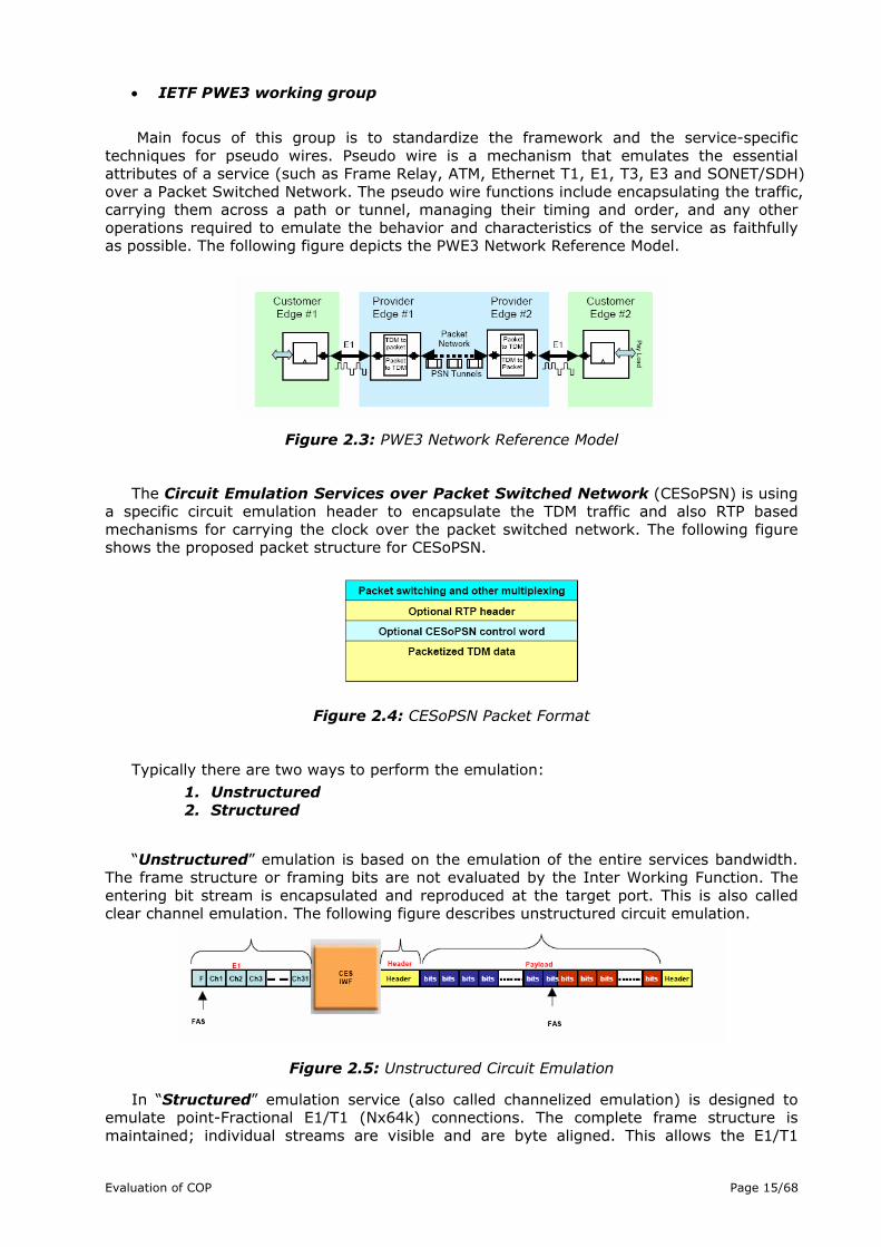
• IETF PWE3 working group

Main focus of this group is to standardize the framework and the service-specific techniques for pseudo wires. Pseudo wire is a mechanism that emulates the essential attributes of a service (such as Frame Relay, ATM, Ethernet T1, E1, T3, E3 and SONET/SDH) over a Packet Switched Network. The pseudo wire functions include encapsulating the traffic, carrying them across a path or tunnel, managing their timing and order, and any other operations required to emulate the behavior and characteristics of the service as faithfully as possible. The following figure depicts the PWE3 Network Reference Model.

Figure 2.3: PWE3 Network Reference Model

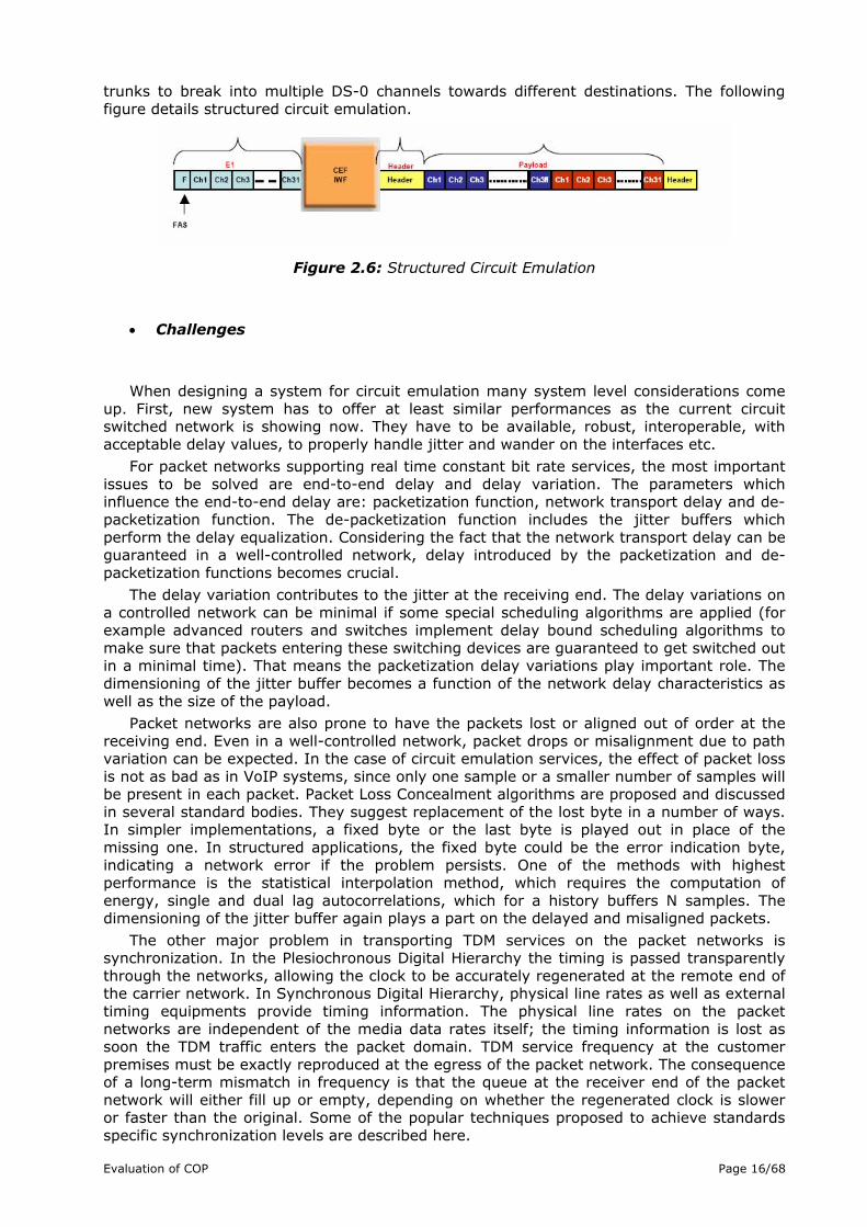
The Circuit Emulation Services over Packet Switched Network (CESoPSN) is using a specific circuit emulation header to encapsulate the TDM traffic and also RTP based mechanisms for carrying the clock over the packet switched network. The following figure shows the proposed packet structure for CESoPSN.

Figure 2.4: CESoPSN Packet Format

Typically there are two ways to perform the emulation:

1. Unstructured 2. Structured

“Unstructured” emulation is based on the emulation of the entire services bandwidth. The frame structure or framing bits are not evaluated by the Inter Working Function. The entering bit stream is encapsulated and reproduced at the target port. This is also called clear channel emulation. The following figure describes unstructured circuit emulation.

Figure 2.5: Unstructured Circuit Emulation

In “Structured” emulation service (also called channelized emulation) is designed to emulate point-Fractional E1/T1 (Nx64k) connections. The complete frame structure is maintained; individual streams are visible and are byte aligned. This allows the E1/T1


trunks to break into multiple DS-0 channels towards different destinations. The following figure details structured circuit emulation.

Figure 2.6: Structured Circuit Emulation

• Challenges

When designing a system for circuit emulation many system level considerations come up. First, new system has to offer at least similar performances as the current circuit switched network is showing now. They have to be available, robust, interoperable, with acceptable delay values, to properly handle jitter and wander on the interfaces etc.

For packet networks supporting real time constant bit rate services, the most important issues to be solved are end-to-end delay and delay variation. The parameters which influence the end-to-end delay are: packetization function, network transport delay and de-packetization function. The de-packetization function includes the jitter buffers which perform the delay equalization. Considering the fact that the network transport delay can be guaranteed in a well-controlled network, delay introduced by the packetization and de-packetization functions becomes crucial.

The delay variation contributes to the jitter at the receiving end. The delay variations on a controlled network can be minimal if some special scheduling algorithms are applied (for example advanced routers and switches implement delay bound scheduling algorithms to make sure that packets entering these switching devices are guaranteed to get switched out in a minimal time). That means the packetization delay variations play important role. The dimensioning of the jitter buffer becomes a function of the network delay characteristics as well as the size of the payload.

Packet networks are also prone to have the packets lost or aligned out of order at the receiving end. Even in a well-controlled network, packet drops or misalignment due to path variation can be expected. In the case of circuit emulation services, the effect of packet loss is not as bad as in VoIP systems, since only one sample or a smaller number of samples will be present in each packet. Packet Loss Concealment algorithms are proposed and discussed in several standard bodies. They suggest replacement of the lost byte in a number of ways. In simpler implementations, a fixed byte or the last byte is played out in place of the missing one. In structured applications, the fixed byte could be the error indication byte, indicating a network error if the problem persists. One of the methods with highest performance is the statistical interpolation method, which requires the computation of energy, single and dual lag autocorrelations, which for a history buffers N samples. The dimensioning of the jitter buffer again plays a part on the delayed and misaligned packets.

The other major problem in transporting TDM services on the packet networks is synchronization. In the Plesiochronous Digital Hierarchy the timing is passed transparently through the networks, allowing the clock to be accurately regenerated at the remote end of the carrier network. In Synchronous Digital Hierarchy, physical line rates as well as external timing equipments provide timing information. The physical line rates on the packet networks are independent of the media data rates itself; the timing information is lost as soon the TDM traffic enters the packet domain. TDM service frequency at the customer premises must be exactly reproduced at the egress of the packet network. The consequence of a long-term mismatch in frequency is that the queue at the receiver end of the packet network will either fill up or empty, depending on whether the regenerated clock is slower or faster than the original. Some of the popular techniques proposed to achieve standards specific synchronization levels are described here.


Figure 2.7: Synchronous Clocking

In a Synchronous service scenario, it is assumed that synchronized clocks are available on each end. The clocking information need not to be transported or derived using packets. The above figure details the Synchronous network circuit emulation.

Timing information need to be transported over the packets or need to be derived from the packets when there are no end-to-end synchronous mechanisms. There are number of methods proposed for regenerating the clock. In the differential clock recovery method, the difference between the service clock (received on the CBR interface) and a network-wide reference clock (like the GPS reference equivalent to Primary Reference Source) is carried over the packets to the destination. At the destination, the information is processed with the reference clock and the source timing is regenerated. It could be depicted by the following figure:

Figure 2.8: Differential Clocking

This clock recovery technique can only be used when a network reference clock is available at the TDM – packet interfaces. Another algorithm uses average packet arrival rate to extrapolate the timing information. Either the data packet arrival rate or specific timing packets from the source at a specific rate can be used for synchronization. The averaging time is chosen both to be long enough not to produce excessive jitter on the recovered clock, and short enough to track any deviations in the source accuracy. The disadvantage of this scheme is that it may be difficult to reproduce a clock which fulfils the wander requirements of the PDH networks. The network delay variation could also be interpreted as the deviation in the source accuracy. The following figure illustrates adaptive clock recovery.

Figure 2.9: Adaptive Clocking

• An Optimal Solution


For an optimal implementation of Circuit Emulation Services, many parameters are of the significant importance: density, power, interfaces, standard compliance etc. One system level solution in the form of block diagram is presented on the figure 2.10

Figure 2.10: System Solution

• Applications

The key applications of Circuit Emulation Services over Packet Networks can be summarized as follows:

• E1/T1 voice/data access services for businesses

• E1/T1 leased line services between businesses

• Backhaul

– Cellular base stations

– DSLAMs (Digital Subscriber Line Access Multiplexer)

– Cable headends

– WiMAX base stations

Metro Ethernet Forum (MEF) has defined four general service types for CESoE functionality.

1. TDM Access Line Services (TALS) in which the MEN provider provisions and

manages TDM leased lines via CESoE, with at least one endpoint terminating in the PSTN

2. TDM Line Service (T-Line) in which the MEN provider provisions and manages TDM private lines via CESoE between enterprise endpoints.

3. Customer-Operated CESoE in which enterprises and other classes of customers manage TDM private lines via CESoE over E-Line (point to point Ethernet) service from MEN provider.

4. Mixed-Mode CESoE in which hybrid combinations of the other three service types are implemented.

1. TDM Access Line Services (TALS)

It enables Metro Ethernet carriers to deliver T1, E1, T3, E3, OC-3, STM-1 based services for voice, Frame relay and ATM over Ethernet networks. TALS supports legacy voice and data applications transparently. Circuit quality matches that of traditional PSTN/circuit based networks.


2. TDM Line (T-line) Services

T-Line service supports all traditional TDM-based private line services over a Metro Ethernet infrastructure.

Enterprise can implement T-lines for:

i. Private/Hybrid frame, ATM, IP, voice and video networking ii. Centralized voice services iii. Private line/toll bypass iv. TDM Backup/Disaster recovery for high uptime and

regulatory compliance v. TDM PBX migration to Ethernet MAN

That way customers get a range of inter-office bandwidth options including:

1. Signal rates from 64 kbps to 51.84 Mbps 2. Point-to-Point and Point-to-Multipoint capability 3. Clear channel capability

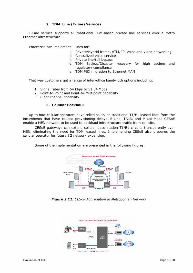
3. Cellular Backhaul

Up to now cellular operators have relied solely on traditional T1/E1 leased lines from the incumbents that have caused provisioning delays. E-Line, TALS, and Mixed-Mode CESoE enable a MEN network to be used to backhaul infrastructure traffic from cell site.

CESoE gateways can extend cellular base station T1/E1 circuits transparently over MEN, eliminating the need for TDM leased lines. Implementing CESoE also prepares the cellular operator for future 3G network expansion.

Some of the implementation are presented in the following figures:

Figure 2.11: CESoP Aggregation in Metropolitan Network


Figure 2.12: Digital Loop Carrier CESoP

Figure 2.13: Multi Tenant/Multi Dwelling Units

Figure 2.14: CESoP over Passive Optical Network

Figure 2.15: CESoP in IP DSLAM

Figure 2.16: CESoP SONET/SDH Extension


Figure 2.17: CESoP over Wireless LAN

• Benefits

CESoE (Circuit Emulation over Ethernet) provides many benefits to existing carriers, competitive operators, mobile/wireless service providers and enterprise users. For instance, it enables providers to offer a complete service portfolio that integrates emerging Ethernet services along with full-featured TDM voice services and private line services (for voice or data). This means that, for the first time, service providers do not have to sacrifice revenues from the widespread and still growing legacy TDM services; they can leverage business models based on all the advantages of Ethernet as a converged packet network. They can use CESoE to provide a group of services for a fixed monthly charge including data VPN access and flat rate local phone service within the network. Carriers can also use CESoE to provide enterprises with interworking to the PSTN at the PSTN central office.

For competitive operators that have built the next generation Ethernet-only networks, circuit emulation ability to enable voice and private line services represents incremental profit opportunities. On the other side for 2G/2.5G cellular providers this is nice opportunity to lower leased line costs and begin migration towards 3G.

Using CESoE enterprise customers can cut their subscriber costs, extend the lives of TDM-based equipment and network architectures.

2.1.7 Conclusion

Constant increasing in the access network traffic forces the service providers to look for options to improve network demands in a reliable, flexible and cost effective way. Circuit Emulation Services over Packet Networks gives one solution how to use existing infrastructure, still enabling service providers to move a packet network based back bone, providing a cost advantage and ensuring the same performance levels as the circuit switched network.


3. Evaluation Methodology

This chapter introduces the test-setup employed to measure performance of CEAs synchronization algorithms. Moreover, the chapter briefly reviews the traffic patterns considered in measurements and the performance metrics used for evaluation.

The Chapter 3 is organized as follows: The section Measurement setup gives detailed description of the system under test. It explains all elements in the setup, their functionality and the complete evaluation process, addressing the main issue in circuit emulation over packets - synchronization. Section is then followed by an analysis of traffic patterns used to test both CEA developed in the CoP project and competitors CEAs. The second part of the Chapter 3, section Metrics for Performance Evaluation defines the most common metrics describing the packet network signal: jitter and wander. The intention is rather to give a short overview of measured properties than to provide a complete tutorial. For more detailed explanations readers are encouraged to look at [7].

3.1 Measurement setup

For the evaluation purposes two Circuit Emulation Adapters (CEAs) are connected together over a Network emulator (see Figure 3.1). A basic test is also done with sending CEA (called “Master”) and receiving CEA (“Slave”) connected back to back. Instead of a network testbed we use a network emulator. As a network emulator we use enhanced NistNet (see [2] ) that has two possibilities to reproduces network dynamics: by accessing internal tables that implement a mathematical model of the emulated network and from traces that were previously captured in a real network. In other words, besides the possibility to work in a standard mode enhanced NistNet is also capable to reproduce wide variety in nature recorded or artificially created traces to simulate events like disconnections, bursts, spanning trees rebuilding and many others. This capability is achieved by replaying large packet delay traces that are previously generated or captured with network probing, simulation, or network calculus Under term “standard mode” we assume originally developed commands to perform packet loss, reordering and duplication, delay and jitter, bandwidth limitations, and network congestion..

PDH signal from PDH generator is given externally to the sending CEA as the input signal. The basic data transfer rate is a data stream of 2.048 Mbit/s. At the sender's side, a CEA packetizes and encapsulates TDM signals and sends them over packet-switched network emulated by the NistNet. As described above emulator influence the signal in the way real network would do. It introduces constant delays and losses, simulates bursts, disconnections and spanning tree rebuilding. At the receiver's side, a receiving CEA de-encapsulates and de-packetizes the incoming packets. Depending on the algorithm for adjusting the receiver buffer play-out rate to the sender packetizing rate, recovered E1 signal would have to have the same frequency as the original signal. This play-out buffer is necessary since frame delays on an Ethernet are highly variable. The output of the receiving CEA is than fed back to the PDH analyzer to evaluate the quality of clock recovery. Ethernet links were using 100 Mbps, full duplex mode. This was necessary for maximum network performance and minimum delays

Albeit the quality of service problem with regards to frame loss and delay is believed to be solvable in metropolitan networks, clock rate synchronization over the Ethernet is still a remaining problem. Highly accurate clock rate synchronization of sending and receiving circuit emulation adapter is necessary to prevent long-term receiver buffer over-/underrun. For VoIP these overflows are not a problem since calls only last for a few minutes. However, base stations are up for weeks and months. As consequence, requirements on clock rate synchronization between sending and receiving circuit emulation adapters are much more stringent. The adjustment may be very difficult at the presence of bursty cross traffic

.


Figure 3.1: Measurement setup: TDM signal from PDH generator is given to the sending CEA as an input. After encapsulation and packetization signal is sent to the receiving CEA

over packet-switched network emulated by the NistNet. Receiving CEA de-encapsulates and de-packetizes the incoming packets. Recovered TDM signal should have to have the same

frequency as the original one. Quality of clock recovery is checked by PDH analyzer

3.1.1 PDH Signal

The PDH signal is one of the important test parameters. Based on the ITU-T G.823 the following guidelines are given

Interface Frequency accuracy

Jitter limit (20…100kHz)

Wander limit

Observation intervals

Traffic interface E1 ±50 ppm 1.50 UI 18 us 64 - 1000 s Synchronization interface E1

±4.6 ppm 1.50 UI 2 us 20 - 2000 s

Table 3.1: Guidelines for 2 Mbps PDH signals

3.1.2 Investigated Network Conditions

In our tests we systematically investigate how CEAs behave under normal, extreme and artificial network conditions. Therefore, we configured the network emulator to work most of the time in trace mode, i.e. to simulate specific events captured in real network environment while standard commands we only need to check CEAs in the presence of constant network delays, statistically varying delays or in the case of lost packets. For that reason we can classify the NistNet setup to be one of the following:

a) Normal Mode b) Extreme Mode c) Artificial Scenarios

a) Normal Mode

The aim of normal mode scenarios is to test the CEAs under normal network conditions, with average daily traffic volume and no strong disturbing interruptions. Such kind of network behavior assumes for example short, light bursts and pulsed events, both with small mean delay values. Delays can also follow some specific probability distribution; in our case delays probability distribution is exponential with given maximum value; such probability model is very common in communication networks.


For testing purposes we use already recorded traces without any special occurrences and some new artificial traces without any special events.

The two typical, real events are:

• Intensive pulsed variations labeled in Test Plan D as: 20000223_1448_etx_rz_8_3m

• Typical short burst labeled as: 20000217_0323_etx_rz_4_3m As artificial trace without special events we have created the following one:

• Delays exponentially distributed up to 200μs with loss ratio 10-8

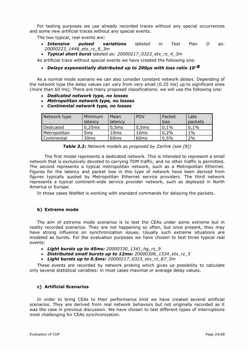
As a normal mode scenario we can also consider constant network delays. Depending of the network type the delay values can vary from very small (0.25 ms) up to significant ones (more than 60 ms). There are many proposed classifications; we will use the following one:

• Dedicated network type, no losses • Metropolitan network type, no losses • Continental network type, no losses

Network type Minimum

latency Mean latency

PDV Packet loss

Late packets

Dedicated 0,25ms 0,5ms 0,5ms 0,1% 0,1% Metropolitan 5ms 10ms 10ms 0,2% 1% Continental 30ms 60ms 60ms 0,5% 2%

Table 3.2: Network models as proposed by Zarlink (see [8])

The first model represents a dedicated network. This is intended to represent a small network that is exclusively devoted to carrying TDM traffic, and no other traffic is permitted. The second represents a typical metropolitan network, such as a Metropolitan Ethernet. Figures for the latency and packet loss in this type of network have been derived from figures typically quoted by Metropolitan Ethernet service providers. The third network represents a typical continent-wide service provider network, such as deployed in North America or Europe.

In those cases NistNet is working with standard commands for delaying the packets.

b) Extreme mode

The aim of extreme mode scenarios is to test the CEAs under some extreme but in reality recorded scenarios. They are not happening so often, but once present, they may have strong influence on synchronization issues. Usually such extreme situations are modeled as bursts. For the evaluation purposes we have chosen to test three typical real events:

• Light bursts up to 45ms: 20000330_1341_hg_rz_9 • Distributed small bursts up to 12ms: 20000306_1334_etx_rz_5 • Light bursts up to 0.5ms: 20000217_0323_etx_rz_67_3m

These events are recorded by network probing which gives us possibility to calculate only several statistical variables: in most cases maximal or average delay values.

c) Artificial Scenarios

In order to bring CEAs to their performance limit we have created several artificial scenarios. They are derived from real network behaviors but not originally recorded as it was the case in previous discussion. We have chosen to test different types of interruptions most challenging for CEAs synchronization.


It is important to point out that in all trace files settling time before the event is set to 300s. This time interval should be long enough for CEAs to adapt to the changed network conditions.

c_1) Disconnections

In networks, disconnections occur rarely but are not impossible. For example when a router gets reconfigured / exchanged or a cable gets damaged. Disconnections can last arbitrarily long. We have chosen several average values to examine CEAs performance under such kinds of interruptions.

Disconnection times are: 10ms, 100ms, 1s, 10s, 100s.

The minimal delay before and after the event is set to 0μs i.e. network is ideal, calm, without any occurrences. Disconnection is than represented with a huge, maximal value supported by NistNet (536870912 decimal value or in binary notation 00100000000000000000000000000000). NistNet is programmed to drop all the packets having delays equal to this specific number.

Remark: A disconnection is the same as a loss rate of 1.

c_2) Spanning tree rebuilding

Sometimes in a network it is necessary to change the routing paths, i.e. to do some traffic reconfiguration. As a consequence spanning tree rebuilding must be deployed. During that period, the packets get very long delays and minimal delays existing in previous configuration, i.e. before event, may be in- or decreased. In other words, after the spanning tree is rebuilt network again operates in standard mode but with high probability minimal delays will have some different values. This is the reason why stable mode before and after tree rebuilding is simulated with delay values different from 0μs. In our case it is 500μs, with changes ± 100μs.

Some interesting delays, occurring during the spanning tree rebuilding, we have chosen to test are: 10ms, 100ms, 500ms, 1s and 5s with changes of minimal delays: -100μs, 0μs, +100μs. Investigated combinations are the following:

• Delay 10ms, delay change -100μs • Delay 10ms, delay change +0μs • Delay 10ms, delay change +100μs • Delay 500ms, delay change -100μs • Delay 500ms, delay change +0μs • Delay 500ms, delay change +100μs • Delay 0ms, delay change -100μs • Delay 1s, delay change +0μs • Delay 5s, delay change +0μs

In all scenarios settling time is set to 300s with default delay 500μs. Spanning tree rebuilding lasts 40ms, 1s, 2s or 5s depending on the delay value during the event. For delay equals 10ms rebuilding lasts 40ms, for 500ms 1s; delays of 0ms and 1s invoke at least 2s for spanning tree rebuilding, while in the case of 5s delay we have chosen also 5s for the event duration. Values for spanning tree duration are chosen from experience i.e. investigating the ratio between delays introduced in the network during the event and measured time needed to go back into the normal operating mode. After the event minimal delay of 500μs stays the same or changes ± 100μs.

c_3) Heavy bursts

Heavy bursts, characterized by fast changing delays, are typical phenomena in communication networks. They are very critical despite of CEAs performance. Like in a normal operating mode burst delay values can also follow some specific probability


distribution. Usually bursts delays are uniformly distributed with the maximum value depending on the network type. The scenarios we have chosen to test are:

• Uniformly distributed delays 0us-100μs • Uniformly distributed delays 0ms-1ms • Uniformly distributed delays 0ms-10ms • Uniformly distributed delays 0ms-100ms

The 300s time interval before burst starts simulates a network without any special occurrences. Minimum delay equals 0μs i.e. it is assumed there are no other interruptions even any constant delays, which is an ideal case. Besides absolute delay values the important parameter for synchronization is burst duration. It influences CEAs stability. For that reason both short and long lasting burst i.e. burst for 100s and 1000s are tested.

c_4) Losses

In networks, losses occur due to many different reasons: due to traffic congestion, misconfiguration or hardware errors. Loss ratios interested for testing are:

• 10-4 • 10-3

• 10-2

3.2 Metrics for Performance Evaluation

The synchronization of two PDH signals can be assessed by looking at their phase variation. Telecommunication standardization sector, the ITU-T for digital systems and networks in the series G.801 suggests evaluating of both phase variations at a rate less than 10Hz and phase variations with frequency components greater than or equal to 10Hz. It should be noted that in these two regions different criteria are used.

3.2.1 Metrics for Jitter UI (Unit Intervals)

Jitter is normally specified and measured as maximum phase amplitude within one or more measurement bandwidth. A single interface may be specified using several different bandwidths since the effect of jitter varies depending on its frequency, as well as its amplitude.

Jitter amplitude is specified in Unit Intervals (UI), such that one jitter UI is one data bit-width, irrespective of the data rate. For example, at a data rate of 2.048 Mbit/s, one UI is equivalent to 488 ns, whereas at a data rate of 155.52 Mbit/s, one UI is equivalent to 6.4 ns.

Jitter amplitude is usually quantified as a peak-to-peak value rather than an rms (root mean square), since it is the peak jitter that causes a bit error made in network equipment.

On the other side rms values are very useful in characterizing and modeling of long line system jitter accumulation, much more than corresponding peak-to-peak values.

3.2.2 Metrics for Wander

Wander measurements are very similar to jitter measurements. However, instead of using an internal reference clock generator, as it is customary in jitter measurement, an external reference clock with minimum intrinsic wander must be supplied. This is due to the fact that phase fluctuations down to nearly 0 Hz would be measured.

Because they involve low frequencies with long periods, wander measurement results can consist of hours of phase information. However, we are more interested in phase


transients, rather than absolute values, so high temporal resolution is also needed. To provide a concise measure of synchronization quality, three wander parameters have been defined and are used to specify performance limits:

a) TIE – Time Interval Error (wander in ns) b) MTIE – Maximum Time Interval Error (related to Peak-to-Peak

wander) c) TDEV – Time Deviation (related to root mean square wander)

Formal mathematical definitions of these and other parameters can be found in Appendix A and B and ITU-T G.801 specification.

a) Time Interval Error (TIE)

The TIE value represents the time deviation of a synchronized receiver clock time t (tested signal) relative to reference sender clock time tref (reference source), typically

measured in ns, i.e. TIE(t) = t – tref. The measurement is always referred to an

Observation Interval τ (in seconds). It is usual to arbitrary set the start of the interval to zero, i.e. TIE(0)=0. For total test period T, therefore TIE gives the phase change since the measurement began.

b) Maximum Time Interval Error (MTIE)

MTIE is a measure that characterizes frequency offset and phase transient. It is again a function of a parameter τ i.e. of the observation interval. The definition (Figure 3.2) is:

MTIE(τ) is the largest Peak-to-Peak TIE (i.e. wander) in any observation interval of the length τ.

Figure 3.2: Functional Definition of MTIE: Maximum peak-to-peak variation of TIE in all the possible observation intervals τ

within a measurement period T

We can also define Relative Maximum Time Interval Error (MRTIE). MRTIE is the maximum peak-to-peak delay variation of an output timing signal with respect to a given input timing signal within an observation time (τ=nτ0) for all observation times of that length within the measurement period (T).

c) Time Deviation (TDEV)

TDEV is a measure of wander that characterizes its spectral component i.e. phase error variation versus the integration time (statistical value). It is calculated from the TIE samples as the maximum TIE deviation for the increasing size of the observation interval τ.

As in the MTIE calculation, it is also a function of the parameter τ i.e. of the observation interval. The definition is:


TDEV(τ) is the rms (root mean square) value of filtered TIE where the bandpass filter (BPF) is centered on a frequency 0.42/τ.

Figure 3.3:. Functional Definition of TDEV: Root mean square deviation of the filtered TIE

We should also point out that TDEV is insensitive to constant phase slope i.e. to frequency offset.

In order to calculate TDEV for a particular τ, the overall measurement period T must be at least 3τ. For an accurate measurement, period T of at least 12τ is required. This is caused by the fact the rms part of TDEV calculation requires sufficient time to get a good statistical average.

For more detailed information about jitter and wander requirements, see Appendix A and B.


4. Evaluation Results

In this chapter we address two important issues: First, we describe in details measurement results obtained by testing the new Circuit Emulation Adapter developed in the CoP project. The overview of the results follows the structure in the Chapter 3, i.e. we discuss the CoP CEA behavior under specific network conditions. In the next part, the CoP demonstrator is compared with tested competitors CEAs available on the market. Chapter 4 ends with the overall conclusion containing the most interesting findings we have discovered during the tests.

4.1 CoP Demonstrator Measurement Results This section lists the most important issues concerning the CoP demonstrator

measurements results. In general we have found very useful features and satisfactory performance. In several tested traffic patterns results show no successful clock recovery. These behaviors are due to the well known issues: arithmetic limitations on the CoP board, delay precision and limited buffer size of the RplTrc (Trace Replicator, see [2]) NistNet which are configuration subjects. Namely, it should be clear that NistNet has a timer set to 121µs. That means, all packets with delays less than or equal to 61µs are immediately forwarded with precision equals to the processing delay which is less than 2µs. But, for packets having delays higher than 61µs, forwarding time, due to discrete interrupts, now equals: actual packet delay ± 61µs, i.e. precision is 121µs. The CoP demonstrator is based on the synchronization algorithm which looks at the real minima in the delay distribution. In the trace mode of the NistNet there are no difficulties due to many real minima. But, in the case of constant network delays higher than 61µs these minima are almost uniformly smeared with the imprecision of 121µs. In other words, there are very few actual minima. That fact causes the problem for synchronization algorithm. The other issue is limited buffer size which is not configured to work with massive packet reordering.

Interesting results will be explained in details while for the rest only important features will be pointed out. Measurements in legends are labeled according to the test plan given in the Appendix D. Sometimes the labels also include additional information about measurements.

4.1.1 Test time and procedure

A very important factor for testing is the observation interval. Based on the Appendix A and B of the MRTIE and TDEV requirements, observation intervals up to 100’000s (28h) are recommended. The proposed traces from section 3.1.2 contain each 3·106 events (delay values). Based on the SAToP standard with a payload size of 256 Bytes/packet there are 1000 packets per second, i.e. one packet per ms. To see the influence of each event, in correspondence one event-one packet, the traces should last for 3000s, i.e. every ms the new trace event should happen. For simplicity reasons and due to the fact that CEA units need some additional time to get settled after reset, we adjust the observation interval for trace based scenarios to be smaller then the trace length, i.e. to be precisely 2500s. The same measurement time holds also for standard NistNet tests.

Every test is performed according to the following procedure:

1. Checking the link sending CEA-receiving CEA in order to see if there is a clear communication between them in the case of no delays or special events on the network; just packet forwarding

2. Starting the selected trace


3. Waiting for the units to be ready according to the synchronization algorithm

4. Starting the MRTIE/TDEV measurement

5. Monitoring the units behavior: boards and interfaces frequencies, measured metrics (MTIE, TDEV, TIE) and link status (bit errors, potential loss of signal synchronization)

6. Noting if there are transmission errors or some unpredictable units’ behavior as well as saving the results for jitter levels, MTIE, TDEV, TIE and other (frequency offset and frequency drift) wander measurements.

4.1.2 Measurement results

d) Normal Mode

As we have mentioned normal mode is represented by some already existing recorded traces without special occurrences, one artificial trace with exponentially distributed delays and specific network models which we have tested with standard NistNet commands.

The results for the traces without any special occurrences (intensive pulsed variations and typical short burst, labeled 20000223_1448_etx_rz_8_3m and 20000217_0323_etx_rz_4_3m respectively) and exponentially distributed delays up to 200µs are as expected: MTIE synchronization mask (see Figure 4.1) is just slightly crossed for short observation periods of up to 10s. That means: looking at the very short time intervals, from 0.02ms up to 10s, we can notice linearly increasing values for Maximum Relative Time Interval Errors with upper bound less than 2000ns. Afterwards, for longer time windows, saturation, i.e. stabilization of MRTIE values is obvious. Put simply, CoP units need some more time, than it is recommended by ITU-T G.823 to adjust the clocks; but afterwards they are pretty stable. This behavior is also seen in TDEV measurements where all curves approach the TDEV mask as observation interval becomes longer and longer (Figure 4.2). This is due to the hardware and software arithmetic limitations of the CoP board which we have mentioned above. For the important long-term stability the CoP CEA shows excellent performance. Additional information about the CoP demonstrator’s performance can be obtained by monitoring values for frequency drift, offset, as well as TIE (examples for the trace without any special occurrences labeled 20000223_1448_etx_rz_8_3m are given on figures 4.5-4.7, together with basic MRTIE and TDEV curves on 4.3 and 4.4 respectively). Careful studying of these figures shows regular changes of the frequency offset frequency drift and TIE values which do not exceed the limits proposed in ITU-T G.823. Maximal frequency offset equals ca. 0.4 ppm, the highest value for frequency drift is approximately 1 ppm/s, while maximal TIE is ca. 2000ns as it is mentioned above.

Link sending CEA – receiving CEA does not show any errors or synchronization losses. Values for jitter measurements are satisfactory inside the limits specified by ITU-T G.823.


Figure 4.1: Normal mode scenarios: MRTIE curves for all important traffic patterns do

not violate the synchronization mask for long-term behavior

Figure 4.2: Normal mode scenarios: TDEV curves approach the synchronization mask for

long-term behavior


Figure 4.3: MRTIE for the intensive pulsed variations: synchronization mask violated only for short observation intervals,

long-term behavior excellent

Figure 4.4: TDEV for the intensive pulsed variations: for longer observation intervals TDEV values approach the limit synchronization curve


Figure 4.5: Frequency offset for the intensive pulsed variations: regular changes with good absolute values

Figure 4.6: Frequency drift for the intensive pulsed variations: regular changes with good absolute values


Figure 4.7: TIE for the intensive pulsed variations: regular changes with good absolute values

The CoP demonstrator’s behavior seen during the measurement for the Dedicated

Network Type with parameters: mean latency 0.5ms, PDV (Packet Delay Variation-approximately equals 4xsigma where sigma is a standard deviation of the delay distribution) also 0.5ms, and no losses is not as good as previous ones. This time MTIE synchronization interface limit is violated (see figures 4.1 and 4.8), but not the MTIE traffic interface one. For detailed explanations of synchronization and traffic interfaces readers are encouraged to look at the subchapters 5.2 and 6.2 of ITU-T G.823.

Explanation for such behavior, including Metropolitan (mean latency 10ms, PDV 10ms) and Continental networks (mean value 60ms, PDV 60ms) scenarios, is given in the introduction of this section and lies in the delay precision of the RplTrc [2]. Results for Metropolitan and Continental networks are not presented because they do not depict the real CoP synchronization stability.


Figure 4.8: MRTIE for Dedicated network type, no losses, mean latency 0.5ms and delay variation 0.5ms: synchronization mask is violated


e) Extreme Mode

As extreme conditions to challenge the CoP CEAs we have chosen some already existing

and recorded traces. Those are bursts already mentioned in the chapter dealing with investigated network conditions i.e.: light bursts up to 45ms (20000330_1341_hg_rz_9), distributed small bursts up to 12ms (20000306_1334_etx_rz_5) and light bursts up to 0.5ms (20000217_0323_etx_rz_67_3m). The results are mainly as we have expected: some errors have occurred in the network; in the case of light burst with maximum value 45ms units have experienced few seconds of signal synchronization loss due to the RplTrc [2] limited buffer size not configured to handle massive packet reordering. Even though short periods of synchronization losses did not have any influence on clock recovery. MRTIE, TDEV and TIE wander measurement results are as good as those in the normal mode scenarios. That means, even under the extreme network conditions long-term synchronization stability of the CoP demonstrator is achieved. Synchronization MTIE mask and corresponding TDEV mask are violated only for short observation windows due to the arithmetic limitations of the CoP boards. All explanations, written in the subchapter above, for CoP CEAs’ behavior in the network without any special occurrences and exponentially distributed delays, are also valid in the case of extreme mode scenarios. MRTIE and TDEV curves are shown below on the Figures 4.9 and 4.10.

Figure 4.9: MRTIE curves for Extreme mode scenarios: long-term synchronization stability


Figure 4.10: Extreme mode scenarios:

TDEV curves approach synchronization limit for long observation intervals

f) Disconnections Not very often but not impossible, network disconnections can happen. CEAs should be

able to handle them with good clock recovery performance. This behavior is proven in the case of the CoP demonstrator. For all tested disconnection times (10ms, 100ms, 1s, 10s and 100s) the results are as expected: sometimes with errors and synchronization losses during the disconnection interrupts. The explanation is the same as the one given for the extreme network conditions: massive packet reordering. Only during disconnections lasting 10s and 100s unavailable seconds occur. This is due to the ITU-T G.821 standard which number of error seconds greater than 10 defines as unavailable. As the figure 4.11 shows, in all tests of interests MRTIE wander curves are below the traffic synchronization mask. For the 10ms, 100ms and 1s events MRTIE values do not even violate the synchronization mask (except for small τ – arithmetic limitations). Similar situation is seen in TDEV measurements: measured curves gradually approach the corresponding mask, i.e. clocks become synchronized for longer observation intervals.


Figure 4.11: Disconnections scenarios: MRTIE curves showing satisfactory synchronization

Figure 4.12: Disconnections mode scenarios: TDEV curves gradually meet the

synchronization limit curve The results for 100s disconnection are not shown on the figures because they are not

realistic, but fully expected. TIE values for disconnection lasting 10s are given in the figure 4.13. The reason for

putting this figure in the thesis is to show regular and satisfactory behavior of the CoP CEA even under strong interrupts. Huge peak around 100s represents the disconnection. It does not match the time in the original trace where this event is happening exactly in 300th second. As we have explained in 4.1.1 this situation is due to the additional CoP demonstrator settling time after the reset. It can easily be seen that soon after the event is finished the CoP CEA is completely back in to standard operation mode with high-grade performance.

Figure 4.13: TIE for10s Disconnections mode scenarios: Peak represents disconnection Good synchronization stability before and after the event

Again the number of unavailable seconds reflects the fact that units go back to the

stable operation mode very quickly after the event in the trace file is finished.


g) Spanning Tree Rebuilding

In this group of tests errors and synchronization losses in the network are expected

considering the fact that minimum delay to occur is 10ms (except of 0ms). In such situations there is no functionality of RplTrc [2]. Depending on how long the spanning tree rebuilding lasts, values for error seconds, i.e. synchronization losses are different; but always in good matching with the events in corresponding traces (example: for tree rebuilding lasting 5s, synchronization is lost for only 7s). In general, a good clock recovery is revealed for all tested scenarios. MTIE and TDEV (see figures 4.14 and 4.15) masks are always violated but this behavior is not influenced by the spanning tree rebuilding, more because of 500µs constant minimal delay before and 400, 500 or 600µs after the event which gives 121µs of imprecision in forwarding delays (see the first paragraph of 4.1).

Figure 4.14: MRTIE curves for Spanning tree rebuilding scenarios:

synchronization mask is violated due to the delay (im)precision of the RplTrc

Figure 4.15: Spanning tree rebuilding scenarios: TDEV curves are still approaching synchronization mask for the long observation intervals


h) Heavy Bursts

Different from disconnections, heavy bursts are very common in communication

networks. This is the reason why it is important to test Circuit Emulation Adapters under these conditions too. We have chosen to test the CoP CEAs’ behavior in a short (100s) and long (1000s) lasting burst environment and for several maximum delay values (200μs, 1ms, 10ms and 100ms). For maximum delays equal 200μs no matter how long burst is neither errors nor synchronization losses are detected. The explanation why devices do not register any errors is found in the 121μs RplTrc [2] timer and uniform distribution of delay values. Most of the packets are forwarded immediately. Clock recovery was very successful for maximum delay values 200μs and 1ms, and not influenced by the burst length.

Figure 4.16: MRTIE curves for Heavy bursts scenarios: very good long term synchronization for short and long burst in the case of small maximal delay values,

satisfactory performance for higher delays if the burst is not too long

Figure 4.17: TDEV curves for Heavy bursts scenarios: for the higher delays, under assumption that burst does not last too long, TDEV curve is higher above the

synchronization mask but still with tendency of approaching it


Interesting results are obtained for the burst scenario with maximum delay value equals 10ms. For the 100s long burst MTIE synchronization mask is violated but the CoP CEAs still show stable behavior for long observation intervals. This is not the case for the burst lasting 1000s or for the maximum delay 100ms. There are simple explanations: First, in real networks burst delays are not uniformly distributed. Looking at the 10ms maximum delay distribution it can easily be concluded that there are many delays which are smaller than 10ms. If the burst is not too long, like in 100s scenario, influence of no functionality for massive reordering and delay imprecision of the RplTrc [2] is still not too strong and the CoP synchronization algorithm can still find many delay minima and perform good clock recovery. But if network delays are high (100ms burst) or the burst last long (1000s), both RplTrc configuration issues have very strong impact on the CoP demonstrator synchronization stability.

i) Losses

In communication networks losses are very common due do many factors: traffic

congestion, misconfiguration or hardware errors. To investigate clock recovery performance

of the CoP demonstrator loss ratios 10-4, 10-3 and 10-2 are chosen. Resistance to losses is a very important criterion in circuit emulation services. The CoP CEAs show excellent robustness due to packet losses. This behavior can easily be seen on the figures below. The CoP CEAs show the same performance as in the traffic patterns without any special occurrences. This feature is very useful.

Figure 4.18: MRTIE values for network with packet losses: high level of robustness and

good long-term synchronization stability


Figure 4.19: TDEV values for network with packet losses: the CoP demonstrator shows

good resistance to packet losses; very high probability to fulfill synchronization requirements for longer observation intervals

4.2 Performances of competitors CEAs The first phase of the CoP project was dedicated to evaluation of competitors’ CEAs

performances. The competitors’ CEAs are called A, B and C and are already available on the market. Industry partner of the CoP project was only interested in their MRTIE wander performances. For that reason this section gives just measurement results for MRTIE values. The performance of each CEA is described in general while the figures show behaviors under different traffic patterns.

4.2.1 CEA of the Competitor A

The performance of the CEA A is on the very high level for almost all investigated

network conditions. The CEA A shows excellent short and long time synchronization stability and robustness due to various traffic patterns and packet losses. MRTIE values do not violate the traffic synchronization mask even for the long lasting burst with high maximum delay value (scenario: 1000s long burst, maximal delay 100ms- figure 4.24). Potential difficulties in clock recovery are found in the Metropolitan and Continental Network scenarios. They can also be explained by the delay imprecision of the RplTrc [2] .Corresponding MRTIE results are not presented in the figures below because they are not the real results.

It should be noted that CEA A offers many parameters to be adjusted in order to achieve good clock recovery. In majority of our tests, the parameter which is adjusted is the size of the jitter buffer. Usually to obtain MRTIE values that fulfill synchronization interface requirements it is necessary to increase the jitter buffer size. The price paid is the higher network delay.


Figure 4.20: Normal mode scenarios: MRTIE curves for all important traffic patterns are

perfectly below the synchronization mask


Figure 4.21: Extreme scenarios: MRTIE curves showing excellent clock recovery


Figure 4.22: Disconnections: For all disconnection times MRTIE values reflect perfect synchronization

Figure 4.23: Spanning tree rebuilding: MRTIE values almost always fulfill

the synchronization interface requirements

Figure 4.24: Heavy bursts: Only for the long lasting burst with high maximum delay

value, MTIE synchronization, but not traffic interface limit is violated


Figure 4.25: Losses: Excellent robustness due to packet losses


4.2.2 CEA of the Competitor B

The CEA B shows better short than long- term synchronization stability. This feature is seen for all tested scenarios. For most investigated traffic patterns MTIE synchronization interface limit, but not the traffic one, is slightly violated. MRTIE values have a tendency to saturate for longer observation intervals. The important characteristic of the CEA B is its robustness due to variety of network conditions, including Metropolitan and Continental Networks. MRTIE values for the Metropolitan Network with parameters: mean delay value 10ms and delay variation 10ms are shown on the figure 4.28. The figure shows that long term synchronization stability is achieved.

Figure 4.26: Normal network conditions: tendency towards synchronization stability for

longer observation intervals; in most cases synchronization mask violated

Figure 4.27: Extreme traffic patterns: MRTIE values


Figure 4.28: MRTIE values for the Metropolitan Network with mean delay 10ms and delay variation 10ms

:long-term behavior tested; synchronization stability achieved

Figure 4.29: Disconnections


Figure 4.30: Spanning tree rebuilding


Figure 4.31: Heavy bursts: difficulties for long lasting burst with high maximal delay value

Figure 4.32: Packet losses: potential synchronization stability for longer observation

intervals, obvious difficulties during measurements


4.2.3 CEA of the Competitor C

The performance of the CEA C is very bad. Only for no special occurrences (intensive pulsed variations and typical short burst) scenarios long-term clock recovery is on the satisfactory level. Under all other investigated network conditions synchronization stability does not fulfill requirements given by ITU-T G.823.

Figure 4.33: MRTIE values for all tested traffic patterns: very bad performance, synchronization mask always violated, for several network scenarios traffic mask also

4.3 The CoP Demonstrator against Competitors CEAs

By careful studying of MTIE values for all evaluated CEAs and for all tested traffic patterns we conclude that:

1. The performance of the CoP CEA is far better than the performance of the CEA C. 2. The performance of the CoP CEA is generally better than the performance of the

CEA B for long-term synchronization stability. This feature is very important for circuit emulation. The synchronization algorithm of the CEA B is more robust to variable network conditions and limited functionality of the RplTrc [2], while the synchronization algorithm implemented on the CoP demonstrator board is much more sensitive to RplTrc configuration.

3. The CEA A performs excellent in almost all traffic scenarios of interest. Both, good short and long-term clock recoveries are proven. Compared to the CoP demonstrator the CEA A shows higher quality level for short-term synchronization stability, while long-term behaviors are comparable. The CEA A is slightly more robust to different traffic scenarios, but also sensitive to delay (im)precision of the RplTrc.


5. Conclusion

The main goal of this thesis is to evaluate the performance of the CEA demonstrator developed in the CoP project. For correct evaluation it is very important to compare the performance of the newly developed CoP CEA against the competitors’ CEAs already available on the market. To test all CEAs we are using various traffic patterns, captured from the real networks or artificially created. From our measurements we conclude that the synchronization algorithm implemented in the CoP demonstrator is of the very high quality for all realistic scenarios including extreme network conditions and packet losses. For several tested network patterns results show no successful clock recovery. These behaviors are due to the well known issues: arithmetic limitations on the CoP board, which can easily be solved in the future development of CEA, delay (im)precision and limited buffer size of the enhanced NistNet (RplTrc), which are configuration subjects. Compared to three tested competitors’ CEAs, the CoP demonstrator shows almost the same, or in one case significantly better, clock recovery. It should be pointed out that the CoP demonstrator is just a demo version of CEA, while the competitors’ CEAs are full products with many parameters to be adjusted in order to achieve satisfactory clock recovery. Further developments in the CoP project should improve the functionalities of the RplTrc as well as they should resolve hardware and software limitations of the CoP board.


Annexes


ANNEX A REQUIREMENTS FOR INPUT FREQUENCY TOLERANCE

In the Plesiochronous Digital Hierarchy (PDH) the timing is passed transparently through the networks, allowing the clock to be accurately regenerated at the remote end of the carrier network.

The input signal frequency of E1 has any value in the range of 2048 kbit/s ± 50 ppm, [G.703]. The digital input port shall be able to tolerate a digital signal that has a rate of change in frequency up to at least 1 ppm/minute [G.823]. However, the Pull-in Range for synchronization purpose is at least: 2048 kbit/s ± 4.6 ppm.

ANNEX B REQUIREMENTS FOR JITTER AND WANDER

Jitter and wander characteristics are organized into limits for jitter and wander tolerance and jitter and wander generation. The jitter and wander tolerance is used to specify the robustness of the data recovery circuits of input ports whereas the jitter and wander generation specifies the timing stability of the output signals.

B.1 Jitter and wander tolerances

The jitter and wander tolerances are beyond the scope of this test plan.

B.1.1 TDM input jitter and wander tolerance of traffic interfaces

The input jitter and wander that can be accommodated by an E1 network interface shall exceed the following limits according to [G.823], chapter 7.1. The levels are expressed in peak-to-peak sinusoidal phase amplitude.

The test sequence to be used is a PRBS of length 215 –1. Thus the signal to encode this sequence is 215 –1 UI (unit interval in time) long. The signal uses a pulse to encode 1 and does nothing to encode 0.

We want to express the tolerance how much a test signal at the input interface can deviate from a reference (ideal signal), i.e. how far rising and falling edges of the test signal can be shifted compared to the reference signal.

Frequency f[Hz]

Requirement [pk-pk phase amplitude] 1 UI = 488 ns

Referenced standard

12u < f ≤ 4,88m 18us G.823 4,88m < f ≤ 10m 0,088 f -1 us G.823 10m < f ≤ 1,67 8,8 us G.823 1,67 < f ≤ 20 15 f -1 us G.823 20 < f ≤ 2,4k 1,5 UI G.823 2,4 < f ≤ 18k 3,6x103 f -1 UI G.823 18 < f ≤ 100k 0,2 UI G.823

Table B-1: Minimum jitter and wander tolerances at traffic input interfaces


Figure B-1: Input jitter and wander tolerance limit

The functional description for measuring input jitter and wander tolerances at a digital interface is provided in [O.171]

The measurement principle is straightforward. What jitter amplitude, using sinewave modulation, at a certain jitter frequency is required to cause the element to violate an error performance criteria? When the test is performed at different jitter frequencies, a complete characteristic is obtained which is compared against the specification mask limit of Figure B-1 (no transformation).

B.1.2 TDM input jitter and wander tolerance of synchronization interfaces

Out of scope of this Thesis (lower priority)


B.2 TDM jitter generation

Jitter characteristics are organized into limits for jitter tolerance and jitter generation. The jitter tolerance is used to specify the robustness of the data recovery circuits of input ports whereas the jitter generation specifies the timing stability of the output signals.

At any network interface, the following output jitter specifications must be met within the defined bandwidth of the measurement filter (Butterworth type). The measurement bandwidth is specified by the lower and the higher cut-off frequencies (-3dB point). At frequencies below the lower cut-off point, the filter has 20 dB/decade roll off characteristic (1st order), while at frequencies above the upper cut-off point the filter is defined as having a 60 dB/decade roll off characteristic (3rd order).

Due to the stochastic nature of jitter, the peak-to-peak values given in this section eventually are exceeded. The requirements shall therefore be fulfilled in at least 99% of all measurements made. I.e. we consider the 99th percentile of these shifts ("phase amplitude") over various measurement time intervals to express the TDM output jitter.

B.2.1 Network limits for TDM output jitter at traffic interfaces

The network limits for the maximum output jitter at any hierarchical interface shall be measured according [G.823], chapter 5.1. This specification must be met at any PDH network node interface (NNI) which works in normal timing mode. These network limits are compatible with the minimum tolerance to jitter that all equipment input ports are required to provide. The specified values below are also valid for PDH synchronization.

The measurement interval lasts 60 seconds.

Measuring filter [Hz]

Peak-to-peak amplitude [UIpp] 1 UI = 488 ns

Referenced standard

20 to 100k (wide-band) 1,50 G.823 700 to 100k 0,2 DTAG 18k to 100k (high-band)

0,2 G.823

Table B-2: Maximum jitter at traffic interfaces

The functional description for measuring output jitter at a digital interface is provided in [O.171].

B.2.2 Network limits for TDM output wander at traffic interfaces

The network limits for the maximum output wander at any hierarchical interface shall be measured according, [G.823] chapter 5.2. This specification must be met at any PDH network node interface (NNI) which works in normal timing mode. These network limits are compatible with the minimum tolerance to wander that all equipment input ports are required to provide.

For the asynchronous mode the maximum observation interval to be considered is 80 seconds.


Observation Interval τ[s]

MRTIE requirement [us]

Referenced standard

0,05 < τ ≤ 0,2 46 τ G.823 0,2 < τ ≤ 32 9 G.823 32 < τ ≤ 64 0,28 τ G.823 64 < τ ≤ 1000 18 G.823

Table B-3: Maximum wander at traffic interfaces

These wander requirements for traffic interfaces comply with ETSI EN 302 084 v1.1.1 (2000-02), chapter 5.2.1.

0.01 0.1 1 10 1k 10k 100k

0.1

1

10

100

MR

TIE

[µs]

329

6418

1k18

Traffic interface

2k2

100k

5.33

SEC interface(MTIE)

0.10.732

7.30.732

Synchronization interface(MTIE)

Freq

. offs

et 4

.6pp

m

Freq

. offs

et 5

0ppm

Freq

. offs

et 5

0ppb

Freq

. offs

et 1

0ppt

0.29

0.052.3

0.10.25

Freq

. offs

et 1

00pp

b

202

2.50.25

Observation Interval t [s]

100

Figure B-2: Output wander limits



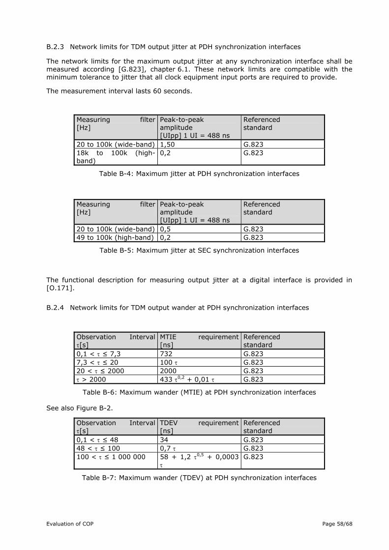
B.2.3 Network limits for TDM output jitter at PDH synchronization interfaces

The network limits for the maximum output jitter at any synchronization interface shall be measured according [G.823], chapter 6.1. These network limits are compatible with the minimum tolerance to jitter that all clock equipment input ports are required to provide.

The measurement interval lasts 60 seconds.



Referenced standard

20 to 100k (wide-band) 1,50 G.823 18k to 100k (high-band)

0,2 G.823

Table B-4: Maximum jitter at PDH synchronization interfaces



Referenced standard

20 to 100k (wide-band) 0,5 G.823 49 to 100k (high-band) 0,2 G.823

Table B-5: Maximum jitter at SEC synchronization interfaces


B.2.4 Network limits for TDM output wander at PDH synchronization interfaces


MTIE requirement [ns]

Referenced standard

0,1 < τ ≤ 7,3 732 G.823 7,3 < τ ≤ 20 100 τ G.823 20 < τ ≤ 2000 2000 G.823 τ > 2000 433 τ0,2 + 0,01 τ G.823

Table B-6: Maximum wander (MTIE) at PDH synchronization interfaces

See also Figure B-2.


TDEV requirement [ns]

Referenced standard

0,1 < τ ≤ 48 34 G.823 48 < τ ≤ 100 0,7 τ G.823 100 < τ ≤ 1 000 000 58 + 1,2 τ0,5 + 0,0003

τ G.823

Table B-7: Maximum wander (TDEV) at PDH synchronization interfaces


Figure B-3: Output wander limit (TDEV) at PDH synchronization interfaces

The measurement period for TDEV should be at least T ≥ 3τ. However, in order to provide accurate results, T > 12τ is recommended.

These wander requirements for synchronization interfaces comply with ETSI ETS 300 462-3 (Jan 97), chapter 7.2.4.


ANNEX C-TRACES

Figure C-4: Trace T01 20000223_1448_etx_rz.dat.txt.8.ana.3m.txt.png



0 0.5 1 1.5 2 2.5 3

x 106

0

20

40

60

80

100

120

140

160

180

200

220

Time(ms)

Del

ay(u

s)

Exponential Delays up to 200us

0 0.5 1 1.5 2 2.5 3

x 106

0

20

40

60

80

100

120

140

160

180

200Exponential Delays up to 200us

Sorted time(ms)

Del

ay(u

s)

Figure C-6: Trace T04 Delay exponentially distributed up to 200us, loss ratio 10-8

FigureC-7: Trace T11 20000330_1341_hg_rz_sent_recv.dat.txt.9.s.ana.txt.png


FigureC-8: Trace T12 20000306_1334_etx_rz_sent_recv.dat.txt.5.s.ana.txt.png



0 0.5 1 1.5 2 2.5 3

x 106

0

1

2

3

4

5

6x 108

Time (ms)

Del

ay (u

s)

disconn 100s

Figure C-10: Trace T22 Disconnection time 100s

0 0.5 1 1.5 2 2.5 3

x 106

0

1

2

3

4

5

6x 106

Time (ms)

Del

ay (u

s)

Sanning Tree Rebuilt 5s change 0us

Figure C-11: Trace T39 Spanning tree rebuilt, delay 5s, delay change 0s 0 0.5 1 1.5 2 2.5 3

6x 106

x 106

0

1

2

3

4

5

Time (ms)

Del

ay (u

s)

Sanning Tree Rebuilt 5s change 0us


0 0.5 1 1.5 2 2.5 3

x 106

0

1

2

3

4

5

6

7

8

9

10x 104 Heavy burst up to 100 ms long 1000s

Time (ms)

Del

ay (u

s)

FigureC-12: Trace T44 Heavy burst, delay 0-100ms, duration 1000s


ANNEX D- TEST PLAN

Traces and Test Signals

Network Behaviour File / Trace Name Trace Description

Trace No.

Trace Type

Duration Trace/Even

t [s]

Mean Latency

PDV [ms]

Packet Loss

Normal 20000223_1448_etx_rz_8_3m no special occurrences T01 REC 3k ≈0 -- 0

Normal 20000217_0323_etx_rz_4_3m no special occurrences T02 REC 3k ≈0 -- 0

Normal exp_delay_200us Delay exponential distributed T04 ART 3k -- …200us 10-3

Normal native NISTNet command Dedicated network type, no losses T05 FIX ∞ 0.5ms 0.5ms 0

Normal native NISTNet command Metropolitan network type, no losses T06 FIX ∞ 10ms 10ms 0

Normal native NISTNet command Continental network type, no losses T07 FIX ∞ 60ms 60ms 0

Extreme 20000330_1341_hg_rz_9 light bursts up to 45ms T11 REC 3k ≈0 ...45ms 0

Extreme 20000306_1334_etx_rz_5 distributed small bursts up to 12ms T12 REC 3k ≈0 ...12ms 0

Extreme 20000217_0323_etx_rz_67_3m light bursts up to 0.5ms T13 REC 3k ≈0 ...0.5m

s 0

Disconn. disconn_10ms Disconnection time: 10ms T21 ART 3k/10m ≈0 -- --

Disconn. disconn_100ms Disconnection time: 100ms T22 ART 3k/100m ≈0 -- --

Disconn. disconn_1s Disconnection time: 1s T23 ART 3k/1 ≈0 -- --



SPTree spann_tree_10ms_change_minus100us Delay 10ms, delay change -100us T31 ART 3k/40m 0.5ms 10ms --

SPTree spann_tree_10ms_change_0us Delay 10ms, delay change +0us T32 ART 3k/40m 0.5ms 10ms --

SPTree spann_tree_10ms_change_plus100us Delay 10ms, delay change +100us T33 ART 3k/40m 0.5ms 10ms --

SPTree spann_tree_500ms_change_minus100us Delay 500ms, delay change -100us T34 ART 3k/1 0.5ms 500ms --

SPTree spann_tree_500ms_change_0us Delay 500ms, delay change +0us T35 ART 3k/1 0.5ms 500ms --

SPTree spann_tree_500ms_change_plus100us Delay 500ms, delay change +100us T36 ART 3k/1 0.5ms 500ms --


SPTree spann_tree_0ms_change_plus100us Delay 0ms, delay change +100us T37 ART 3k/2 0.5ms 0 --

SPTree spann_tree_1s_change_plus0us Delay 1s, delay change +0us T38 ART 3k/2 0.5ms 0 --

SPTree spann_tree_5s_change_plus0us Delay 5s, delay change +0us T39 ART 3k/5 0.5ms 0 --

Burst heavy_bursts_upto200us_long100s Uniform distributed delays 0us-200us T41 ART 3k/100 ≈0 ..200us --

Burst heavy_bursts_upto200us_long1000s Uniform distributed delays 0us-200us T41a ART 3k/1000 ≈0 ..200us --

Burst heavy_bursts_upto1ms_long100s Uniform distributed delays 0ms-1ms T42 ART 3k/100 ≈0 …1ms --

Burst heavy_bursts_upto1ms_long1000s Uniform distributed delays 0ms-1ms T42a ART 3k/1000 ≈0 …1ms --

Burst heavy_bursts_upto10ms_long100s Uniform distributed delays 0ms-10ms T43 ART 3k/100 ≈0 …10ms --

Burst heavy_bursts_upto10ms_long1000s Uniform distributed delays 0ms-10ms T43a ART 3k/1000 ≈0 …10ms --

Burst heavy_bursts_upto100ms_long100s Uniform distributed delays 0ms-100ms T44 ART 3k/100 ≈0 ..100ms --

Burst heavy_bursts_upto100ms_long1000s Uniform distributed delays 0ms-100ms T44a ART 3k/1000 ≈0 ..100ms --

Losses native NISTNet command Loss ratio to test: 10-2 T51 FIX ∞ ≈0 -- 10-2



tion of COP /68

Evalua

Bibliography

[1] Rainer Baumann, Ulrich Fiedler, “Implementing CoP’s Circuit Emulation Adapter

Demonstrator", TIK Report Nr. 221, June, 2005 [2] Rainer Baumann, Ulrich Fiedler, “ReplTrc: A Tool for Emulating Real Network

Dynamics", TIK Report Nr. 218, June, 2005 [3] Ullas Kumar, “Circuit Emulation Over Packet Networks”, www.zarlink.com [4] Slobodan Milijevic, “Timing Synchronization in Packet Networks”,

www.zarlink.com [5] Tim Frost, “Circuit Emulation Over Packet Switched Networks”, www.zarlink.com [6] ITU-T G.823, “The control of jitter and wander within digital network which are

based on the 2048 kbit/s hierarchy”, March, 2000 [7] Tektronix, “Performance Assessment of Timing and Synchronization in

Broadband Networks”, 1996, Tektronix UK [8] www.zarlink.com [9] www.metroethernetforum.org

Title, WHO 6. July 2006 /68

evaluating circuit emulation adapters

Documents