evaluating hfc network readiness for deployment of … docsis network... · evaluating hfc network...
TRANSCRIPT
© 2016 Society of Cable Telecommunications Engineers, Inc. All rights reserved.
Evaluating HFC Network Readiness for Deployment of D3.1 Technology and Services
An Operational Practice prepared for SCTE/ISBE by
Dean Stoneback, SCTE/ISBE Member Senior Director, Engineering and Standards
SCTE/ISBE 140 Philips Road, Exton, PA 19341-1318
484-252-2363 [email protected]
Jack Moran, SCTE/ISBE Member Distinguished Expert of Cable Access Research
Huawei [email protected]
Lamar West, PhD, SCTE/ISBE Member Owner
LEW Consulting, LLC [email protected]
Daniel Howard, SCTE/ISBE Member Director, Consulting Services, Energy, Efficiency and Environmental Solutions
Hitachi Consulting Corp. [email protected]

© 2016 Society of Cable Telecommunications Engineers, Inc. All rights reserved. 2
Table of Contents
Title Page Number
Introduction ________________________________________________________________________ 4 1. Executive Summary _____________________________________________________________ 4 2. Scope ________________________________________________________________________ 4 3. Background ___________________________________________________________________ 5
Operational Practices ________________________________________________________________ 5 4. Example Goals for HFC Readiness Activities _________________________________________ 5 5. General Aspects of HFC Readiness: Logistics, Planning and Overall Optimiztion of the
Downstream and Upstream Paths __________________________________________________ 8 5.1. Logistics and Planning ____________________________________________________ 8 5.2. Downstream Optimization _________________________________________________ 10 5.3. Upstream Optimization ___________________________________________________ 11
6. Tests and Measurements for HFC Readiness Activities ________________________________ 13 6.1. Key Performance Metrics _________________________________________________ 13 6.2. Required Equipment _____________________________________________________ 14 6.3. Calibration and Equipment Preparation ______________________________________ 15 6.4. Detailed Procedures _____________________________________________________ 15
6.4.1. Histograms: MER, MTR, GDV, Amplitude Ripple, and Other DOCSIS CPE Metrics _______________________________________________________ 15
6.4.2. Laser Dynamic Range via In-service NPR ____________________________ 17 6.4.3. Determination of Laser Margin Required to Prevent Clipping ______________ 20 6.4.4. Plant Sweeps __________________________________________________ 27 6.4.5. Piecemeal Upstream Sweeps via DOCSIS Carriers _____________________ 28 6.4.6. Intermodulation Distortion Characterization via Unmodulated Carriers ______ 30 6.4.7. Transient Noise Characterization ___________________________________ 30 6.4.8. Leakage Characterization at Planned D3.1 Frequencies _________________ 30 6.4.9. Phase Noise via High Order QAM Constellation Analysis and Carrier
Injection with PNM ______________________________________________ 31 6.4.10. Peak to Average Power Ratio (PAPR) _______________________________ 31 6.4.11. Contention Minislot Sufficiency _____________________________________ 33 6.4.12. Upstream Power Spectral Distribution and Alignment ___________________ 34
7. Coexistence of DOCSIS 3.1 and MoCA in the Home Environment ________________________ 38
Conclusion ________________________________________________________________________ 38
Appendix A: Comparison of DOCSIS 3.1 to 3.0 ___________________________________________ 38
Abbreviations ______________________________________________________________________ 41
Bibliography & References ___________________________________________________________ 42
List of Figures
Title Page Number
Figure 1 - NPR curves for different upstream laser technology using a 9 dB margin for interference [Howard, Howald & Moran] 11
Figure 2 - MER distribution from Comcast, 22M devices [Urban] 15
Figure 3 - Downstream received signal level distribution before and after 1 GHz plant upgrade [Benevides] 17
© 2016 Society of Cable Telecommunications Engineers, Inc. All rights reserved. 3
Figure 4 – Major Elements of NPR Curve [SCTE 119] 18
Figure 5 - Nine Carrier – 16-QAM – 6.4 MHz Carriers Input Power to Node versus EQ-MER (Similar to NPR Curve) given 25 km of Fiber 19
Figure 6 - Test Setup For In-service NPR Measurement 20
Figure 7 - Transient Noise Interference 21
Figure 8 – Upstream Loaded with DOCSIS Carriers 22
Figure 9 – Additional Carriers Added 22
Figure 10 – Distortion Visible Due to Increased Carrier Levels 23
Figure 11 – Upstream MER vs. Total Input Power 23
Figure 12 - Upstream MER vs. Total Input Power With 4 dB Less Ingress Margin 24
Figure 13 - Upstream MER vs. Total Input Power With 6 dB Less Ingress Margin 25
Figure 14 – Upstream Interference Noise, Example 1 25
Figure 15 - Upstream Interference Noise, Example 2 26
Figure 16 – Upstream Laser Clipping Due To Impulse Noise 27
Figure 17 - Group Delay Variation As a Function of Cascade Depth [SCTE Impairments] 28
Figure 18 - Typical Data Available from PNM Upstream Characterization Per Channel [SCTE PNM] 29
Figure 19 - Example Spectrum Capture From CM Showing Direct Pickup of LTE Signal 31
Figure 20 - PAPR As a Function of OFDM Subcarriers [Wambach]) 32
Figure 21 – Simulation of Large Numbers of Collisions in Contention Minislots 33
Figure 22 – Simulation of Increasing Numbers of Collisions in Contention Minislots 34
Figure 23 – Constant Power per Carrier vs. Constant Power per Hertz 34
Figure 24 - Constant Power per Carrier – Four Identical Channel Width Carriers Bonded 35
Figure 25 - Constant Power per Carrier – Eight Identical Channel Width Carriers Bonded 36
Figure 26 - Constant Power per Carrier – Four Carriers, Two Channel Widths 36
Figure 27 - Constant Power per Hertz – Four Bonded Carriers, Two Channel Widths 37

© 2016 Society of Cable Telecommunications Engineers, Inc. All rights reserved. 4
Introduction
1. Executive Summary
Target Audience: Network engineers, network architects, access network engineers, critical facility engineers, outside plant technicians, field and installation technicians, and training content developers.
What are the immediate and long-term benefits of adopting it?
Maximizing the capacity/spectral efficiency of HFC networks when D3.1 is deployed Reducing customer care calls, truck rolls/repeat truck rolls, and the mean time to repair (MTTR) Ensuring initial deployment of D3.1 equipment functions properly and does not degrade existing
services and equipment
What are some of the key points of this operational practice?
Performing a complete RF network characterization using test equipment, existing monitoring solutions, proactive network maintenance (PNM) capabilities in cable modems and settops, or a combination of these methods
Characterizing and optimizing laser margins on upstream/downstream using passive and active measurements to enable greater occupancy of existing spectrum
Developing histograms of modulation error ratios (MERs) and other key performance indicators (KPIs) of the network to determine types of Data Over Cable Service Interface Specification (DOCSIS) 3.1 profiles that can be used, and estimate the resulting capacity
Sweeps of upstream and downstream to determine optimal cyclic prefix settings for DOCSIS 3.1 signals
Verifying the upstream capacity and configuration, e.g. contention minislots, are ready for additional downstream traffic
Determining optimal signal placement and spacing between DOCSIS 3.1 and legacy signals on the network
Setting signal levels to optimize spectral efficiency in bits/s/Hz Moving from a constant power per carrier upstream configuration to constant power per Hz or
other power spectral density distributions to optimize capacity
What can you do to achieve maximum benefit from implementing this operational practice? Customize it for your workforce/cable network specifics. Implement the practices, keeping track of key performance indicators (KPIs) both before and after the implementation to insure it is meeting the business goals of the cable operator.
How can you learn more about this operational practice? Join the Network Operations Subcommittee (NOS) working group in the SCTE/ISBE Standards Program and assist in revisions and updates to this document. Visit http://www.scte.org/standards, or email: [email protected] for more information.
2. Scope
This operational practice covers tests, measurements, and overall processes by which cable operators can ensure their HFC networks are optimized for the rollout of DOCSIS 3.1 technology. Not covered are
© 2016 Society of Cable Telecommunications Engineers, Inc. All rights reserved. 5
activities such as expanding the downstream RF spectrum of the HFC network or moving the upstream-downstream split point, which is covered in a CableLabs report [CAB] and a previous SCTE/ISBE paper [Moran1]. Coexistence of DOCSIS 3.1 (D3.1) and Multimedia over Coax Alliance (MoCA) is discussed briefly in section 7 and is also addressed in another SCTE/ISBE paper [Thompson].
While D3.1 technology was designed for existing plants with little or no changes required to the existing DOCSIS 3.0 (D3.0) HFC network, there are nonetheless simple and more extensive testing and measurement activities cable operators can perform to maximize the capacity D3.1 provides. This is the mission of the SCTE/ISBE Special Working Group on HFC Readiness and this document.
Finally, the proactive network maintenance (PNM) technologies referred to in this document are typically those that are currently available with D3.0 customer premises equipment (CPE). New D3.1 PNM features and measurements will occasionally be mentioned, but detailed procedures for using them will be saved for a subsequent version of this document.
3. Background
HFC readiness for D3.1 is about maximizing the capacity achieved and minimizing the potential issues that might arise from deploying D3.1 in current cable networks. In addition, HFC readiness entails determining which new operational practices, key performance indicators (KPIs), tools and training are needed to optimize customer satisfaction, plant health, and robustness using D3.1. The operational practices in this document are focused on all of these aspects, but in particular the goal of maximizing the capacity achieved with D3.1 deployment. Both downstream and upstream characteristics of the HFC network should thus be optimized as part of HFC readiness activities.
DOCSIS 3.1 signals, capabilities, and features are significantly different from those of DOCSIS 3.0. Appendix A is a partial description of key differences between the two specifications to aid in training the workforce as part of HFC readiness, and is expected to expand as this document evolves in the special working group.
Operational Practices
4. Example Goals for HFC Readiness Activities
The high level goals of D3.1 deployment are well known, the most important of which is to increase network capacity overall and also enabling greater than 1 Gbps downstream burst rates with a more robust signaling scheme to all customers. And very importantly, to be able to do so without requiring extensive plant modifications thereby effecting the upgrade to D3.1 cost-effectively. There are also new features in D3.1 such as active queue management that improve the latency performance, and of course a plethora of new, built-in proactive network maintenance (PNM) features [Currivan & Wolcott]. Finally, all new technology deployment plans have the underlying goal of preventing any negative impact of the new technology deployment on existing signals and services.
The goals of an HFC readiness program can be extensive. At the highest level, all signaling schemes provide their greatest possible capacity, namely the spectral efficiency in bits per second per Hz (bps/Hz) of RF spectrum when integrated across the entire RF spectrum, when the channel is as clean and free of impairments as possible. But the network equipment in place must also have the capability to support the new signaling scheme to the greatest extent possible.
© 2016 Society of Cable Telecommunications Engineers, Inc. All rights reserved. 6
In this light, a partial list of specific HFC readiness goals that have been given in the various industry forums and publications is listed below, grouped into eight major categories, with an indication of whether the category is primarily test and measurement (T&M) or analysis:
1. Characterization of Current Networks (T&M) a. Develop a histogram of modulation error ratio (MER) (both unequalized and equalized),
codeword error (CWE) ratios (corrected and uncorrected) and other KPIs to plan D3.1 configurations and deployment
b. Sweep the plant to identify, locate and if possible correct large microreflections in the downstream that may affect D3.1 cyclic prefix requirements
c. Perform detailed composite intermodulation distortion (CID) characterization of the network to ensure it is possible to fully load the downstream without significant clipping
d. Measure laser dynamic range to determine the proper system laser margin required vs. signal to noise performance and set the operating points for lasers and amplifiers
e. Sweep the plant for ingress and leakage that causes D3.1 to interact with external signals such as LTE
f. Characterize plant issues that may cause frequency/timing errors to which D3.1 and higher order modulations can be more sensitive
g. Characterize the system group delay variation, especially near band edges, to determine viability of using D3.1 near or even within band edges and/or rolloff regions
2. Identification of Network Improvements (if any) (analysis) a. Assess need for/benefits of downstream laser replacements such as with better distributed
feedback (DFB) cooled downstream lasers b. Assess need for/benefits of upstream laser replacements, such as with higher powered
upstream lasers c. Assess need for/benefits of passive and RF active replacements d. Determine the incremental benefits achievable through plant spectrum extensions. e. Determine which network improvements, if any, should be done before D3.1 deployment
to optimize network capacity and which, if any, should be done afterwards f. Identify low performing outliers in network/device performance and develop a plan to
mitigate their issues and tighten the overall distribution á la Deming quality control methods, e.g. mitigating the lowest MER cases.
g. Evaluate changes needed to the plant balance/alignment to support full loading and future growth of capacity and burst rates
h. Identify network improvements that can minimize the number of different D3.1 modulation profiles used initially (e.g., how to tighten up the distribution of MERs from cable modems and move the average upward)
3. Configuration Planning/Capacity Optimization (analysis) a. Optimize currently deployed D3.0 systems in the process, in particular the upstream
which may remain primarily D3.0 for some time b. Determine the best profiles (modulation orders, cyclic prefixes, windowing, etc.) to use
for D3.1 for a given cable operator’s individual networks and/or architectures and assess the capacity provided thereby relative to the robustness of the profile
c. Determine the best D3.1 deployment strategy to minimize disruption and maximize capacity (configurations, signal placement and next phase of plant actions)
© 2016 Society of Cable Telecommunications Engineers, Inc. All rights reserved. 7
d. Determine how closely D3.1 carriers can be placed next to existing carriers (as a function of D3.1 windowing parameters) and also to band edges
e. Determine the new D3.1 operating KPIs/metrics to use for network monitoring, assessment, and alarming
4. Interoperability Testing (T&M) a. Ensure complete compatibility with existing HFC architecture, especially if RF over
Glass ( RFoG) is used [SCTE 174] b. Ensure that adding D3.1 to downstream does not overload upstream with requests on
large nodes (collisions in contention mini-slots can cause clipping) c. Assess the system peak to average rower ratio (PAPR) before and after D3.1 deployment
to validate laser margins used and RFoG functionality
5. Field Testing (T&M) a. Verify long term network performance and stability of D3.1 on actual networks b. Verify performance predictions and stability of speeds provided c. Verify no interoperability issues with existing D3.0 services, devices, and maintenance
procedures d. Verify whether D3.1 can be used in the rolloff regions of the network e. Finalize D3.1 configuration parameters for full deployment
6. Update NetOps (analysis) a. Modify and augment existing network metrics, measurements, baselines and KPI’s b. Develop new processes needed or enabled by D3.1, even if only in sparse deployments c. Identify which features of D3.1 proactive network maintenance (PNM) are most desired
for initial use d. Identify new test equipment or test equipment upgrades needed for maintaining D3.1 in
the network
7. Workforce Training a. Develop workforce training programs for D3.1 and OFDM, such as the SCTE/ISBE D3.1
Bootcamp b. Develop or update PNM training programs for 3.1 PNM technology and measurements c. Develop new sales and customer care training programs for D3.1 deployment
8. Business Planning (market selection, speed tier offerings; analysis) a. Determine the best initial markets in which to deploy D3.1 (although this may be
completely market-driven, not network readiness-driven) b. Determine the best transition path to complete D3.1 deployment c. Optimize energy efficiency, e.g. kWh/TB consumed via D3.1 deployment (an
SCTE/ISBE Energy 2020 goal) d. Develop capacity and burst rate/speed tier expectations for sales teams

© 2016 Society of Cable Telecommunications Engineers, Inc. All rights reserved. 8
5. General Aspects of HFC Readiness: Logistics, Planning and Overall Optimiztion of the Downstream and Upstream Paths
5.1. Logistics and Planning
Successful plant readiness activities potentially affect the entire network, and thus require engineering planning and project/budget management, organization communications, company commitment, supply chain planning and coordination, and workforce training. As with any major engineering effort associated with the deployment of new technology, the usual top level areas for planning and logistics apply, for example [Benivides]:
Engineering activities: Overall project management and planning and may also include repair and construction, technology selection, contractor/field tech selection and training
Procurement/logistics: Vendor and contractor RFP’s, equipment purchase and materials distribution
Customer service/impact: Identification of any service interruption/impacts from HFC readiness activities, planning for customer care responses, and coordination with call center agents
Network operations: Training for field tests and measurements, new network equipment/technology, additional truck rolls required, and post migration monitoring
And note that it is advisable to do a partial or full suite of current plant and device monitoring and characterization tasks before and after any service-impacting measurements to ensure that all modems and set top boxes are back online from any outage that resulted from testing. This is especially important if plant issues that should be repaired are detected during HFC readiness activities, which often happens in any plant characterization effort. These issues in the outside plant (OSP) can include, but are not limited to [Benevides], [SCTE Impairments], [Hranac]:
Failed line connectors Damaged or missing end of line terminators Damaged (chewed, kinked or cracked) cable or corroded cable Burned taps Network design maps not current (for example, amplifiers that have been moved from their
design location) and lack of design maps for some locations like multiple dwelling units Damaged/missing chassis terminators on directional coupler, splitter, or amplifier unused ports Loose center conductor seizure screws Unused tap ports not terminated Poor isolation in splitters, taps and directional couplers Use of so-called self-terminating taps at feeder ends-of-line Defective or damaged actives or passives Some traps and filters have poor return loss in the upstream
From a high level planning perspective, there are tests and characterizations of HFC readiness that can and should be done first over the entire footprint of the cable operator’s network, such as the MER and other key histogram tests described later, using either PNM technology or widely deployed centralized monitoring systems. In this manner, an overall sense of the distribution of network health can be gathered and used to plan the more detailed labor and/or test equipment intensive tests such as laser margin testing. For these tests, since it is not feasible to test all nodes within a cable operator’s network, the SCTE/ISBE
© 2016 Society of Cable Telecommunications Engineers, Inc. All rights reserved. 9
Special Working Group on HFC Readiness has recommended that cable operators use the data on network health from the entire footprint to select at least four sites that represent the diversity of network architectures and/or performance conditions as follows:
Typical top performing network site: One that is well-maintained as evidenced by current KPI data, well shielded and bonded/grounded coax plant (as evidenced by leakage data) with a flat thermal noise background on the upstream and minimal impulse/burst noise seen the vast majority of the time. A plant that is nearly identical to a clean laboratory environment, and may for example use the most fiber-deep architecture such as N+0 or N+1.
Average performing typical network site: Typically maintained & shielded coax plant that is representative of the largest number of coax plants in the operator’s footprint, with some steady state ingress, transient impulse/burst noise and micro-reflections present on the upstream for example and some incidence of LTE or other leakage seen on the downstream. Node plus a few actives, e.g. N+3 type plant if it is found throughout the cable operator’s footprint.
Relatively challenged network site: A system where most of the MERs are in the lower half of the overall distribution, or where the largest number of low MER modems are found. Often a coax plant with some un-terminated tap ports and/or poor grounding/bonding practices; several coax breaks in need of repair, and significant levels of steady state ingress, transient impulse/burst noise, and micro-reflections seen throughout the network. Often a site with the largest number of actives per node and/or the oldest portion of the cable operator’s footprint.
Advanced deployment network site: A fourth site that represents either the first planned market deployment from a competitive perspective, or alternately a site that represents a targeted upgrade to the newest and most advanced architecture, for example a remote PHY node with passive coax, or other remote architectures. To reiterate, these advanced architectures are not necessary for leveraging the benefits of D3.1; the technology was designed to use plants without any major modifications to them. However, advanced distributed access architectures (DAA) are seen in one sense as a possible means of achieving the highest possible spectral efficiencies from D3.1 (8192 or even 16,384 QAM), and if such architectures are available, then the opportunity to test their HFC readiness for the highest spectral efficiencies possible with D3.1 should not be ignored.
Given the variation seen in KPIs from measurements, it is recommended that for each of the four diverse sites just described, at least 8 nodes per site should be tested, again striving for maximum diversity in the nodes selected in order to bound the domain of performances seen in existing networks.
Finally, the importance of using new PNM features in D3.1 technology cannot be overstated. Since as of this writing, D3.1 modems and cable modem termination system (CMTS) or converged cable access platform (CCAP) systems are available, it is now possible to deploy D3.1 headend systems and a sparse deployment of advanced D3.1 modems with early phase implementations of these PNM features (or alternately, use cable modems specifically designed for use as remote characterization devices as proposed in [Moran2]) and accomplish all three HFC readiness activities:
Characterizing HFC readiness for full deployment of D3.1. Deploying modems in specific locations to monitor plant health such as at the end of line, in
power supplies, or in locations such as those recommended in [Moran2]. Training the workforce ahead of full deployment on the next generation of PNM technology (as
well as proofing out the new PNM tools in the process and developing a tool-adoption plan for 3.1-based PNM technology) which will be used by all field technicians when D3.1 is fully deployed.
© 2016 Society of Cable Telecommunications Engineers, Inc. All rights reserved. 10
This can be done well-ahead of full scale deployment and provides the cable operator with a means of getting much more diverse, robust and granular PNM data on their plant health early on in the D3.1 deployment process.
5.2. Downstream Optimization
Downstream challenges to achieving maximum spectral efficiency include micro-reflections, group delay variation at RF band edges, LTE ingress, available laser dynamic range for fully loading the downstream spectrum, and composite intermodulation distortion (CID). In systems with an all-digital downstream, CID appears not as narrowband composite triple beat (CTB) or composite second order (CSO) interference that could be easily mitigated by D3.1’s subcarrier nulling/QAM order reduction capability, but rather as a raised broadband noise floor [Howard]. This CID noise floor cannot be cancelled and thus limits the MER and therefore the maximum spectral efficiency possible. Proper design rules on network alignment are even more important in D3.1 downstream optimization so that nonlinearities do not produce a raised noise floor. The noise floor from composite intermodulation distortion is best characterized via the noise power ratio test [SMRP NPR], which is also now part of the planned PNM capabilities in D3.1 through a combination of nulling a block of subcarriers and then doing an RF band spectrum capture to characterize the noise floor.
The total input power into the laser in the head-end has received few modifications over the past several years to reflect the ever expanding downstream bandwidth demands. A reevaluation of the linearity requirements of the downstream (as well as upstream) lasers may be in order for the laser to attain the performance objectives, and these are, in order of importance:
Total input power into the laser: Keeping the total input power relative to the capability of the laser such that the peak characteristics of the total composite signal hitting the laser will not clip the laser a significant percentage of the time, e.g. more than 20% of the minimum symbol duration on the network [SMRP Peak-Avg].
Distribution of power among the various downstream services: It has been observed that there exists quite a large variance worldwide in power settings between analog and digital carriers, and even among the types of digital carriers on the downstream. Determining the recommended level that digital carriers should be transmitting will be important to optimizing the downstream, especially since D3.1 technology may alter previous assumptions and rationale used for power level planning.
HFC amplifier cascade depth: Given the previous discussion about CID potentially limiting the maximum achievable MER and thus spectral efficiency on the HFC network, the number of amplifiers in cascade following the node will have a definite impact on the downstream capacity achievable with D3.1.
Unused tap termination policy and unused drop coaxial cable termination policy: As is the case in the upstream, the HFC plant should be tightened against all interference signals for optimum downstream capacity. New tap technology may change the general approach to terminations and shielding effectiveness, and thus they should also be considered if they afford significant capacity and performance improvements.
All the optimizations listed above will maximize the performance of the system for D3.1 operation. It is worth a reminder that, even without network optimization, D3.1 will, in general, perform at least as good as D3.0 when deployed. The optimizations described in this paper are designed to achieve the maximum
© 2016 Society of Cable Telecommunications Engineers, Inc. All rights reserved. 11
possible performance of the D3.1 network, resulting in significant improvements in capacity and reliability over D3.0.
5.3. Upstream Optimization
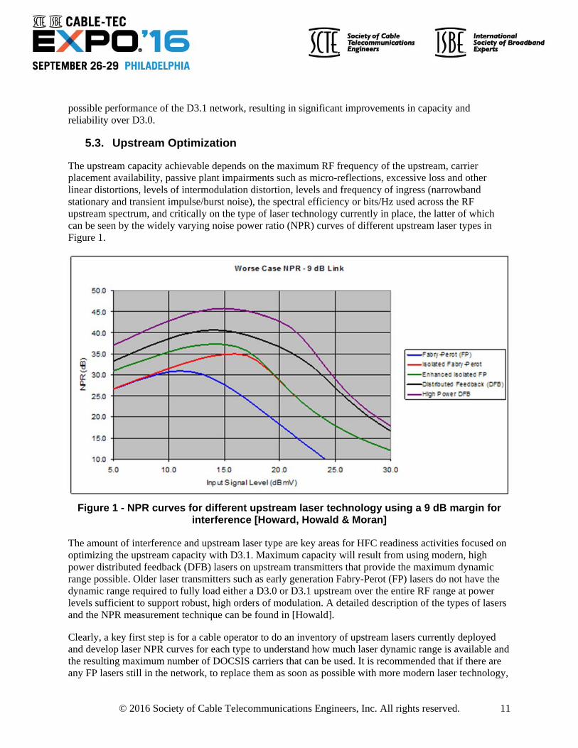
The upstream capacity achievable depends on the maximum RF frequency of the upstream, carrier placement availability, passive plant impairments such as micro-reflections, excessive loss and other linear distortions, levels of intermodulation distortion, levels and frequency of ingress (narrowband stationary and transient impulse/burst noise), the spectral efficiency or bits/Hz used across the RF upstream spectrum, and critically on the type of laser technology currently in place, the latter of which can be seen by the widely varying noise power ratio (NPR) curves of different upstream laser types in Figure 1.
Figure 1 - NPR curves for different upstream laser technology using a 9 dB margin for interference [Howard, Howald & Moran]
The amount of interference and upstream laser type are key areas for HFC readiness activities focused on optimizing the upstream capacity with D3.1. Maximum capacity will result from using modern, high power distributed feedback (DFB) lasers on upstream transmitters that provide the maximum dynamic range possible. Older laser transmitters such as early generation Fabry-Perot (FP) lasers do not have the dynamic range required to fully load either a D3.0 or D3.1 upstream over the entire RF range at power levels sufficient to support robust, high orders of modulation. A detailed description of the types of lasers and the NPR measurement technique can be found in [Howald].
Clearly, a key first step is for a cable operator to do an inventory of upstream lasers currently deployed and develop laser NPR curves for each type to understand how much laser dynamic range is available and the resulting maximum number of DOCSIS carriers that can be used. It is recommended that if there are any FP lasers still in the network, to replace them as soon as possible with more modern laser technology,

© 2016 Society of Cable Telecommunications Engineers, Inc. All rights reserved. 12
preferably a high power DFB type. Note that even if the operator is beginning a migration to digital returns via remote PHY or other digital return technologie, there is still a potential dynamic range issue with for example remote PHY due to the limited dynamic range of the analog to digital converter used in technology.
To maximize the laser dynamic range, one must also minimize the laser margin required for transient interference impairments and composite signal peaking. The high peak-to-average power ratio (PAPR) of higher order modulation and/or higher complexity waveforms like orthogonal frequency-division multiple access (OFDMA), and even collisions of grant requests in contention mini-slots, can rob the upstream of precious laser headroom that would be better used for improving the MER of all carriers. This is true whether advanced time division multiple access (ATDMA) or OFDMA is used on the upstream.
Thus, a close examination of the upstream laser properties under fully loaded conditions is recommended, as well as procedures for characterizing, locating, and eliminating sources of plant impairments that lead to high levels of impulse/burst noise on the upstream. Intermittent (loose) connections in particular can allow the ingress of considerable upstream interference, and can potentially cause an entire node from operating properly for a short period, even though a single home is the source of the intermittent connection. However, it is now possible to use PNM technology to identify such intermittent connections and fix them [Hunter].
Based on the additional PNM measurements thereby provided, the recommended approach for testing the upstream under fully loaded conditions is to use actual DOCSIS carriers to load up the upstream, rather than injecting noise, e.g. This allows testing of all three key upstream characteristics simultaneously: upstream laser dynamic range, presence of significant amounts of upstream impulse/burst noise (via significant codeword error ratios), and the possibility of significant numbers of collisions from insufficient contention mini-slots on the upstream that would cause increased clipping incidents. Following coarse readiness determination via this technique, more granular data can be obtained via specific measurements and procedures that are also given or referenced in this document.
Finally, the upstream signal levels themselves should be carefully planned and coordinated so that optimal use of available laser margin is achieved. The method recommended for this is the constant power per Hz method, as opposed to the constant power per carrier method [Howald].
In summary, an upstream optimization process for HFC readiness involves the following:
1. Determine the maximum theoretical capacity possible on currently deployed HFC upstream lasers by fully loading a typical upstream configuration (initially in the lab, and then verifying it in the field) that is free of impairments of any form.
2. Characterize the reduction in capacity that results from different laser upstream power margins being added.
3. Characterize the level of steady state ingress and transient impulse/burst noise present on the upstream as currently maintained to determine the value of upstream laser margin that is required to prevent clipping for current maintenance levels. Then, if excessive margins are required, develop a process using PNM and/or centralized monitoring solutions to eliminate these impairments to reduce the margin required to avoid clipping.
© 2016 Society of Cable Telecommunications Engineers, Inc. All rights reserved. 13
4. Develop a power and modulation profile for DOCSIS carriers on the upstream that maximizes the capacity under the various upstream profiles conditions discovered from the MER histogram and PNM (or centralized monitoring system) data collection, and thereby minimizes the potential for disrupting existing services as new carriers are added and the laser upstream dynamic range is fully utilized.
If the cable operator discovers the margins required for impairments are too large to achieve market goals for speed tiers, an aggressive plan of tightening the HFC network can be put in place including, among other things, proactively eliminating sources of steady state ingress and transient impulse/burst noise, minimizing group delay variation via reducing the cascade depth, assuring proper amplitude tilt, reducing the magnitude and number of micro-reflections in the network by replacing damaged sections or components, replacing older coax, especially partially shielded series 59 drop lines, and ensuring proper termination and grounding/bonding practices are implemented throughout the network.
Finally in the longer term, although not in scope of this document, for homes that are particularly troublesome in terms of generating upstream interference, several options exist and have been discussed in various forums such as: use of low spectrum filters on the input to upstream lasers; rewiring homes; modifying CPE placement, upgrading home set top boxes to modern MoCA media gateways with two F-connectors that isolate the home coax network from the rest of the cable network (however note that this effectively becomes a point of entry device, which could impact Wi-Fi coverage unless separate Wi-Fi access points are used within the home) ; using Wi-Fi access to the home from cable Wi-Fi hotspots; RFoG or other fiber-to-the-home solutions; and moving the upstream split point to open up cleaner spectrum for DOCSIS carriers.
6. Tests and Measurements for HFC Readiness Activities
6.1. Key Performance Metrics
This section will include the key performance metrics to be measured and will provide a brief overview of the theory behind each one.
Bit error ratio (BER) and associated metrics such as errored seconds (ES) and severely errored seconds (SES)
Carrier-to-noise ratio (CNR) Modulation error ratio (MER) and derivative metrics such as average MER, standard deviation of
MER, minimum and maximum MER over ensembles and over time per modem, corner quadrant MER (since this is where amplifier compression and phase noise issues are most prominent) and so on
Codeword error ratio (CWER), RC Maximum group delay variation (GDV) Noise power ratio (NPR) Main tap ratio (MTR) of the pre-equalization process, and related equalizer tap metrics Achievable order of modulation for reliable communications Required power margin for upstream and downstream laser operation Number of laser clipping events and/or mean time between laser clipping events Incidence of impulse/burst noise events above a given level and for longer than 20% of the
minimum signal period
© 2016 Society of Cable Telecommunications Engineers, Inc. All rights reserved. 14
In addition, histograms of the above metrics, e.g. MER, should be plotted for all cable operator CPE devices, for individual systems/markets, and per node within a system, and possibly versus various parameters such as plant age, plant repair activity, temporal history, construction nearby, etc. so that long term trends in plant impairments can be proactively identified in the future and repaired before they cause customer complaints.
In addition to the above network performance metrics, others that relate to the workforce or effectiveness of ingress elimination can be collected. These may include metrics such as:
Mean time to repair (MTTR) ingress cause after detection and location; Mean time between repeated detections on a node, system or region; Average number of ingress detections per node, system, or region.
On the qualitative front, RF spectrum and quadrature amplitude modulation (QAM) constellation snapshots of both the cable upstream, from the CMTS or CCAP (and with D3.1, from the CM), and also on the cable downstream from the CM (using full band/full spectrum capture capabilities), should be collected and analyzed as an additional means of assessing the average health of the network, portions of the network that may require attention as part of an HFC readiness program, and specific issues that should be addressed over time to optimize D3.1 performance.
6.2. Required Equipment
It is now possible to use existing CMTS/CCAP equipment and CM (or DOCSIS-based STBs) to monitor and characterize plant impairments and, in the absence of existing centralized monitoring solutions deployed throughout the network, this is the preferred method since these devices are already in use in the network. Further, PNM technology will be significantly enhanced in D3.1, to include upstream spectrum capture at the CM, triggered captures, and greater resolution in impairment identification and location.
Additionally, traditional cable network monitoring equipment such as the following can be used to assess HFC readiness:
Spectrum analyzer (SA) and QAM-based SA Digital sampling oscilloscope (DSO) Fast Fourier transform (FFT) real time analyzer Vector signal analyzer (VSA) Handheld digital signal analyzers Centralized monitoring systems (e.g. the Viavi PathTrakTM, Arris ServAssureTM, or the VeEx
VeSionTM systems, among others)
For capturing stationary narrowband ingress such as HF or FM radio stations, a spectrum analyzer is often the easiest to use, while for transient ingress events, including impulse and burst noise events, a time domain capture from a DSO or FFT real time analyzer is often better.
There is also a need for some of the intermodulation tests below to inject carriers into the HFC network, which can be done via any of the following
RF signal generator (5-1000 MHz) DOCSIS 3.1 CMTS (unmodulated pilot tones)
© 2016 Society of Cable Telecommunications Engineers, Inc. All rights reserved. 15
Arbitrary waveform generator (for upstream multicarrier intermodulation characterization)
6.3. Calibration and Equipment Preparation
All equipment used for measurements should be properly calibrated and maintained per the manufacturer’s instructions.
6.4. Detailed Procedures
6.4.1. Histograms: MER, MTR, GDV, Amplitude Ripple, and Other DOCSIS CPE Metrics
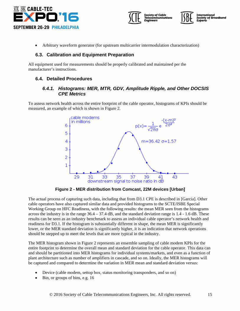
To assess network health across the entire footprint of the cable operator, histograms of KPIs should be measured, an example of which is shown in Figure 2.
Figure 2 - MER distribution from Comcast, 22M devices [Urban]
The actual process of capturing such data, including that from D3.1 CPE is described in [Garcia]. Other cable operators have also captured similar data and provided histograms to the SCTE/ISBE Special Working Group on HFC Readiness, with the following results: the mean MER seen from the histograms across the industry is in the range 36.4 – 37.4 dB, and the standard deviation range is 1.4 - 1.6 dB. These results can be seen as an industry benchmark to assess an individual cable operator’s network health and readiness for D3.1. If the histogram is substantially different in shape, the mean MER is significantly lower, or the MER standard deviation is significantly higher, it is an indication that network operations should be stepped up to meet the levels that are more typical in the industry.
The MER histogram shown in Figure 2 represents an ensemble sampling of cable modem KPIs for the entire footprint to determine the overall mean and standard deviation for the cable operator. This data can and should be partitioned into MER histograms for individual systems/markets, and even as a function of plant architecture such as number of amplifiers in cascade, and so on. Ideally, the MER histograms will be captured and compared to determine the variation in MER mean and standard deviation versus:
Device (cable modem, settop box, status monitoring transponders, and so on) Bin, or groups of bins, e.g. 16

© 2016 Society of Cable Telecommunications Engineers, Inc. All rights reserved. 16
Frequency (when multiple bonded D3.0 carriers are used) Time (diurnal and seasonal) Location Climate Plant architecture/particulars (cascade depth, RFoG, etc.) NetOps policies (if they vary market to market)
In this manner, the variation in KPIs that can be improved due to plant architecture and NetOps policies, for example, can be isolated from the natural variation that is inevitable. The former can be used over time to increase the network capacity provided by D3.1, while the latter points to the range of modulation profiles required.
In particular, it is recommended to capture the MER histogram data over time to ensure that the values seen in the histogram are stable and thus truly indicate what order of modulation the modem would typically support in D3.1. From a signal processing and analysis point of view, if time variations in KPIs are identical to ensemble variations, the variable is ergodic and thus for example, individual markets can use time averages to aggressively seek to improve the KPIs and the results would apply equally well to the larger ensemble of the entire cable operator’s footprint. However, many experts do not expect such KPIs to be ergodic, believing KPIs will be a strong function of plant architecture, age, climate, and NetOps policies. This should be confirmed via a comprehensive histogram analysis program during HFC readiness efforts.
Downstream MER is not the only KPI for which histograms are recommended in order to assess current network health and HFC readiness for D3.1. Others include, but are not limited to:
Main tap ratio (MTR) Maximum group delay variation per widest possible signal bandwidth (max GDV) Maximum amplitude ripple, both in channel and across the entire RF spectrum used Downstream receive levels and codeword error ratios (CWER) as a proxy for BER Upstream transmit and receive levels Upstream CWER
Note that the CWER is given by the total number of uncorrectable codewords divided by the total codewords sent (the sum of correctable, unerrored and uncorrectable codewords) collected by the following MIBs:
docsIfSigQUnerroreds docsIfSigQCorrecteds docsIfSigQUncorrectables
Many of these other KPIs may also have normal distributions, for example the histograms shown in Figure 3 of downstream received signal level were measured by a cable operator before and after expanding the plant RF spectrum to 1 GHz.

© 2016 Society of Cable Telecommunications Engineers, Inc. All rights reserved. 17
Figure 3 - Downstream received signal level distribution before and after 1 GHz plant upgrade [Benevides]
From a longer term viewpoint, the histograms should be seen as part of a Deming-type quality improvement program: first characterize the statistical variation the network, and then look at the outliers below the mean to figure out how to tighten up the distribution, and above the mean to figure out how to make system-wide changes that improve the mean for the entire ensemble. In the above figure, after upgrading the plant to 1 GHz RF, the mean signal level went up by about 0.6 dB due to plant improvements made in the process of making the upgrade, but the standard deviation also went up by about 0.5 dB. The process should thus be repeated to tighten the distribution back up, identifying outliers, fixing issues, and so on.
6.4.2. Laser Dynamic Range via In-service NPR
Currently, the SCTE recommends doing NPR measurements only for equipment that is out of service using a broadband noise generator with notch filters [SMRP NPR], [SCTE 119]. In this section, a set of new in-service procedures will be given that will allow characterization of plant non-linearity and readiness for fully loaded upstreams and downstreams using both D3.0 and also D3.1 signals. This procedure can also be used in laboratory or other out of service settings. This procedure description is for testing upstream laser nonlinearity, however it could also be modified to use for downstream laser nonlinearity testing, especially if a D3.1 modem is used.
When enough D3.0 SC-QAM or D3.1 carriers are injected into the upstream, the distribution of amplitudes turns out to be nearly Gaussian, and thus the DOCSIS signal loading is not only a good
25 Sept: Mean = ‐2.19 dBmV, Std = 5.07 dBmV
26 Sept: Mean = ‐1.67 dBmV, Std = 5.58 dBmV (24 hours after network upgrade completed)
© 2016 Society of Cable Telecommunications Engineers, Inc. All rights reserved. 18
approximation of a truly noise-like waveform, but is more realistic in terms of the actual signals to be transmitted over the HFC network. And the use of actual D3.1 signals improves this approximation via both the higher order modulation and the expected slightly higher PAPR of OFDMA as compared to TDMA.
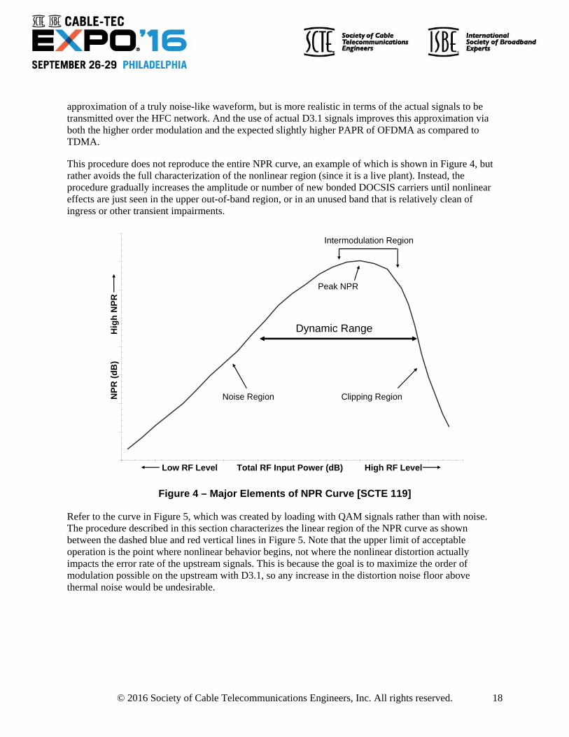
This procedure does not reproduce the entire NPR curve, an example of which is shown in Figure 4, but rather avoids the full characterization of the nonlinear region (since it is a live plant). Instead, the procedure gradually increases the amplitude or number of new bonded DOCSIS carriers until nonlinear effects are just seen in the upper out-of-band region, or in an unused band that is relatively clean of ingress or other transient impairments.
Figure 4 – Major Elements of NPR Curve [SCTE 119]
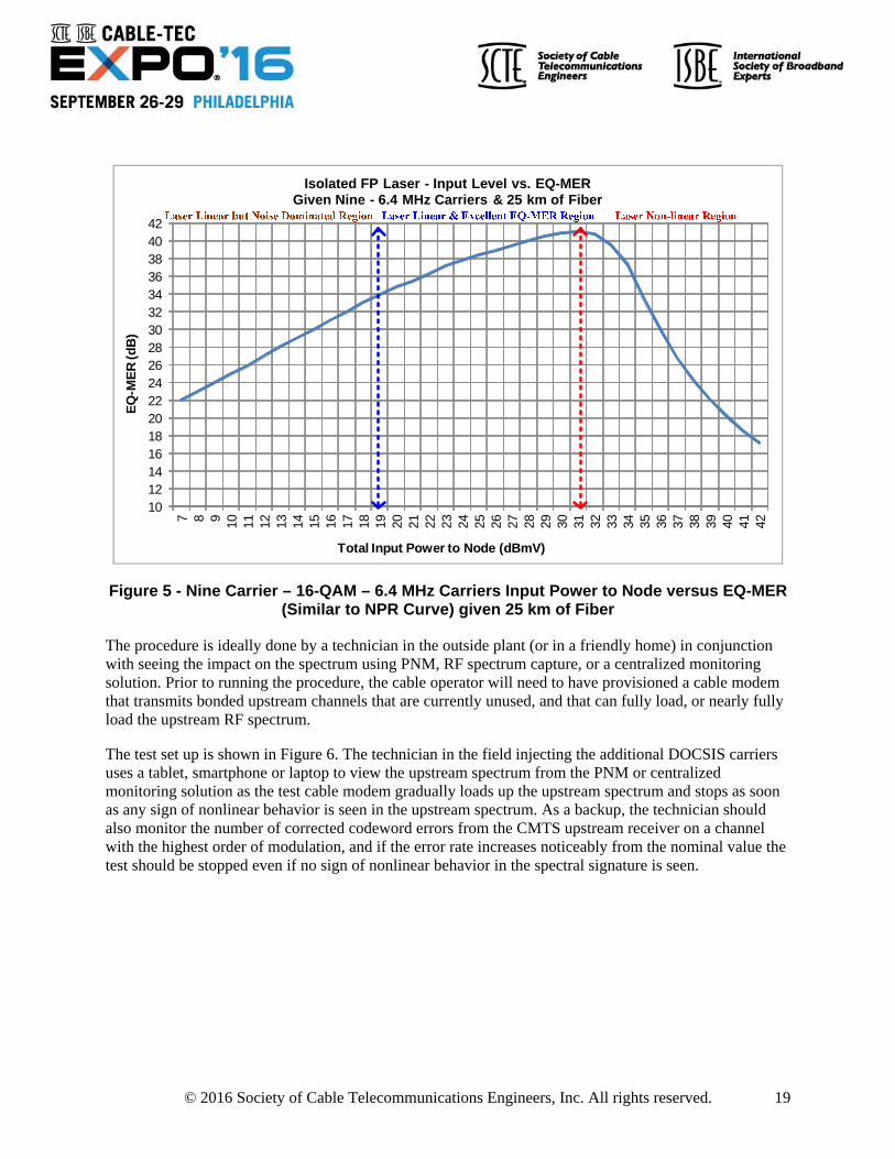
Refer to the curve in Figure 5, which was created by loading with QAM signals rather than with noise. The procedure described in this section characterizes the linear region of the NPR curve as shown between the dashed blue and red vertical lines in Figure 5. Note that the upper limit of acceptable operation is the point where nonlinear behavior begins, not where the nonlinear distortion actually impacts the error rate of the upstream signals. This is because the goal is to maximize the order of modulation possible on the upstream with D3.1, so any increase in the distortion noise floor above thermal noise would be undesirable.
Low RF Level Total RF Input Power (dB) High RF Level
NP
R (
dB
)
Hig
h N
PR
Dynamic Range
Clipping RegionNoise Region
Peak NPR
Intermodulation Region
© 2016 Society of Cable Telecommunications Engineers, Inc. All rights reserved. 19
Figure 5 - Nine Carrier – 16-QAM – 6.4 MHz Carriers Input Power to Node versus EQ-MER (Similar to NPR Curve) given 25 km of Fiber
The procedure is ideally done by a technician in the outside plant (or in a friendly home) in conjunction with seeing the impact on the spectrum using PNM, RF spectrum capture, or a centralized monitoring solution. Prior to running the procedure, the cable operator will need to have provisioned a cable modem that transmits bonded upstream channels that are currently unused, and that can fully load, or nearly fully load the upstream RF spectrum.
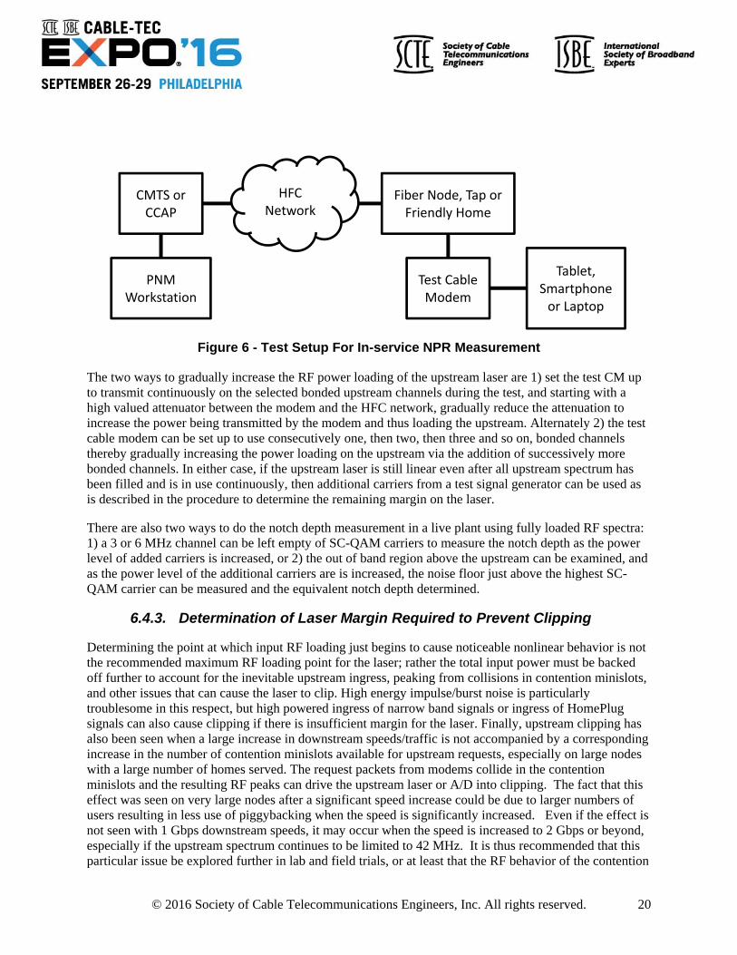
The test set up is shown in Figure 6. The technician in the field injecting the additional DOCSIS carriers uses a tablet, smartphone or laptop to view the upstream spectrum from the PNM or centralized monitoring solution as the test cable modem gradually loads up the upstream spectrum and stops as soon as any sign of nonlinear behavior is seen in the upstream spectrum. As a backup, the technician should also monitor the number of corrected codeword errors from the CMTS upstream receiver on a channel with the highest order of modulation, and if the error rate increases noticeably from the nominal value the test should be stopped even if no sign of nonlinear behavior in the spectral signature is seen.
1012141618202224262830323436384042
7 8 9 10 11 12 13 14 15 16 17 18 19 20 21 22 23 24 25 26 27 28 29 30 31 32 33 34 35 36 37 38 39 40 41 42
EQ
-ME
R (d
B)
Total Input Power to Node (dBmV)
Isolated FP Laser - Input Level vs. EQ-MERGiven Nine - 6.4 MHz Carriers & 25 km of Fiber
© 2016 Society of Cable Telecommunications Engineers, Inc. All rights reserved. 20
Figure 6 - Test Setup For In-service NPR Measurement
The two ways to gradually increase the RF power loading of the upstream laser are 1) set the test CM up to transmit continuously on the selected bonded upstream channels during the test, and starting with a high valued attenuator between the modem and the HFC network, gradually reduce the attenuation to increase the power being transmitted by the modem and thus loading the upstream. Alternately 2) the test cable modem can be set up to use consecutively one, then two, then three and so on, bonded channels thereby gradually increasing the power loading on the upstream via the addition of successively more bonded channels. In either case, if the upstream laser is still linear even after all upstream spectrum has been filled and is in use continuously, then additional carriers from a test signal generator can be used as is described in the procedure to determine the remaining margin on the laser.
There are also two ways to do the notch depth measurement in a live plant using fully loaded RF spectra: 1) a 3 or 6 MHz channel can be left empty of SC-QAM carriers to measure the notch depth as the power level of added carriers is increased, or 2) the out of band region above the upstream can be examined, and as the power level of the additional carriers are is increased, the noise floor just above the highest SC-QAM carrier can be measured and the equivalent notch depth determined.
6.4.3. Determination of Laser Margin Required to Prevent Clipping
Determining the point at which input RF loading just begins to cause noticeable nonlinear behavior is not the recommended maximum RF loading point for the laser; rather the total input power must be backed off further to account for the inevitable upstream ingress, peaking from collisions in contention minislots, and other issues that can cause the laser to clip. High energy impulse/burst noise is particularly troublesome in this respect, but high powered ingress of narrow band signals or ingress of HomePlug signals can also cause clipping if there is insufficient margin for the laser. Finally, upstream clipping has also been seen when a large increase in downstream speeds/traffic is not accompanied by a corresponding increase in the number of contention minislots available for upstream requests, especially on large nodes with a large number of homes served. The request packets from modems collide in the contention minislots and the resulting RF peaks can drive the upstream laser or A/D into clipping. The fact that this effect was seen on very large nodes after a significant speed increase could be due to larger numbers of users resulting in less use of piggybacking when the speed is significantly increased. Even if the effect is not seen with 1 Gbps downstream speeds, it may occur when the speed is increased to 2 Gbps or beyond, especially if the upstream spectrum continues to be limited to 42 MHz. It is thus recommended that this particular issue be explored further in lab and field trials, or at least that the RF behavior of the contention
PNM Workstation
CMTS or CCAP
HFC Network
Fiber Node, Tap or Friendly Home
Test Cable Modem
Tablet, Smartphone or Laptop
© 2016 Society of Cable Telecommunications Engineers, Inc. All rights reserved. 21
minislots is closely monitored via triggered upstream captures to determine if the peak to average ratio is increasing as more subscribers take and use the higher speed services.
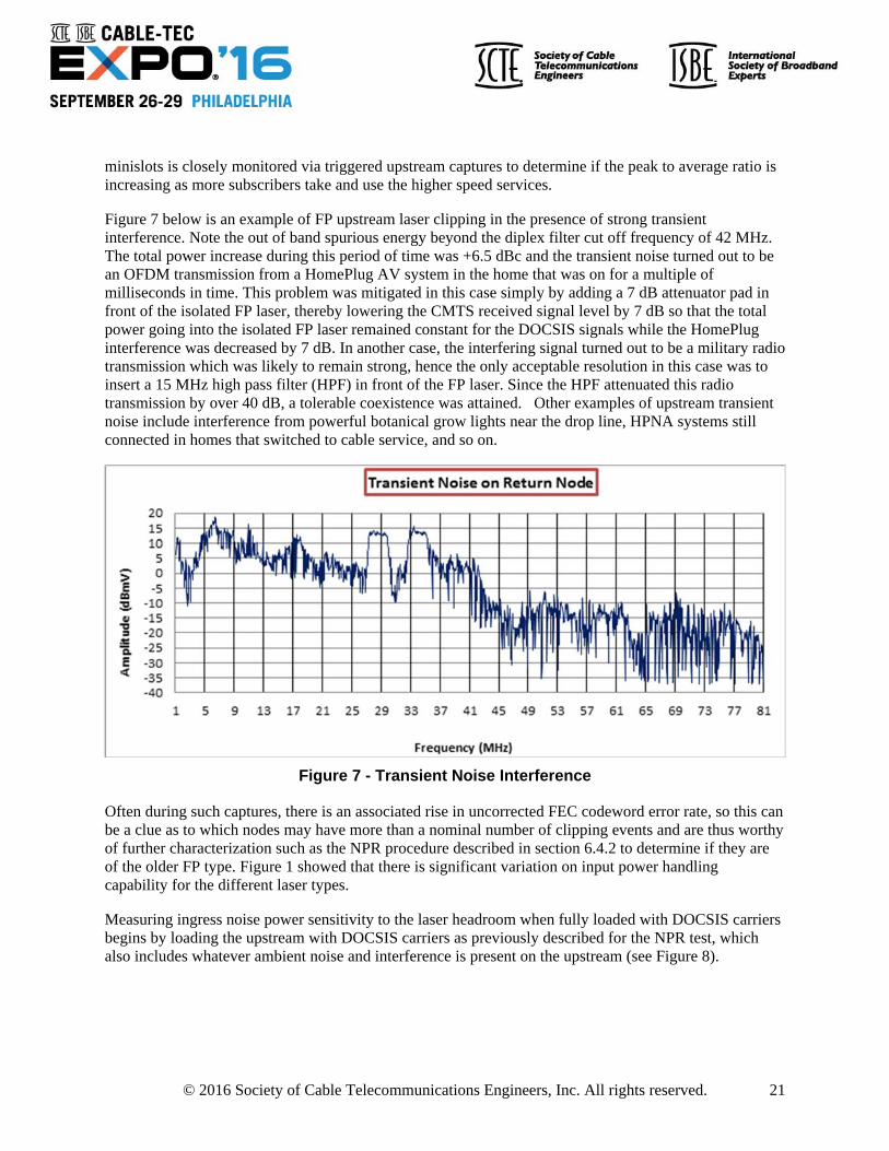
Figure 7 below is an example of FP upstream laser clipping in the presence of strong transient interference. Note the out of band spurious energy beyond the diplex filter cut off frequency of 42 MHz. The total power increase during this period of time was +6.5 dBc and the transient noise turned out to be an OFDM transmission from a HomePlug AV system in the home that was on for a multiple of milliseconds in time. This problem was mitigated in this case simply by adding a 7 dB attenuator pad in front of the isolated FP laser, thereby lowering the CMTS received signal level by 7 dB so that the total power going into the isolated FP laser remained constant for the DOCSIS signals while the HomePlug interference was decreased by 7 dB. In another case, the interfering signal turned out to be a military radio transmission which was likely to remain strong, hence the only acceptable resolution in this case was to insert a 15 MHz high pass filter (HPF) in front of the FP laser. Since the HPF attenuated this radio transmission by over 40 dB, a tolerable coexistence was attained. Other examples of upstream transient noise include interference from powerful botanical grow lights near the drop line, HPNA systems still connected in homes that switched to cable service, and so on.
Figure 7 - Transient Noise Interference
Often during such captures, there is an associated rise in uncorrected FEC codeword error rate, so this can be a clue as to which nodes may have more than a nominal number of clipping events and are thus worthy of further characterization such as the NPR procedure described in section 6.4.2 to determine if they are of the older FP type. Figure 1 showed that there is significant variation on input power handling capability for the different laser types.
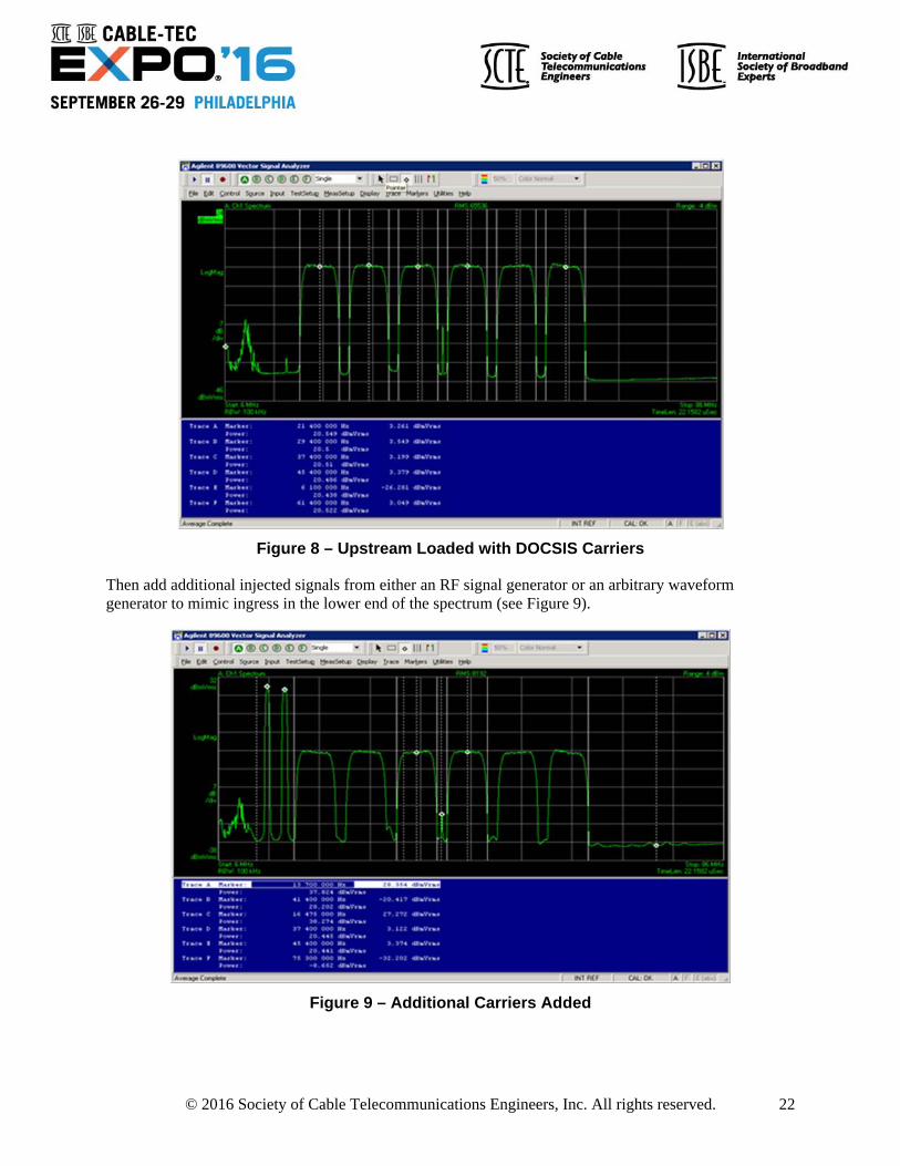
Measuring ingress noise power sensitivity to the laser headroom when fully loaded with DOCSIS carriers begins by loading the upstream with DOCSIS carriers as previously described for the NPR test, which also includes whatever ambient noise and interference is present on the upstream (see Figure 8).
© 2016 Society of Cable Telecommunications Engineers, Inc. All rights reserved. 22
Figure 8 – Upstream Loaded with DOCSIS Carriers
Then add additional injected signals from either an RF signal generator or an arbitrary waveform generator to mimic ingress in the lower end of the spectrum (see Figure 9).
Figure 9 – Additional Carriers Added
© 2016 Society of Cable Telecommunications Engineers, Inc. All rights reserved. 23
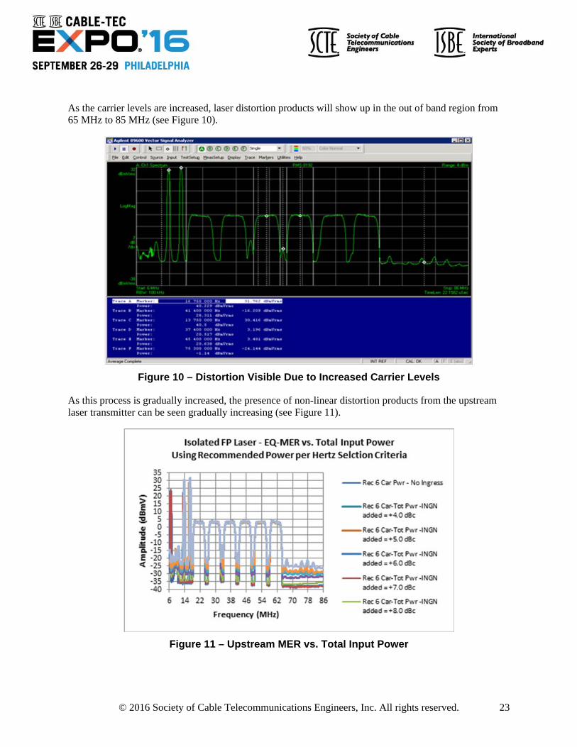
As the carrier levels are increased, laser distortion products will show up in the out of band region from 65 MHz to 85 MHz (see Figure 10).
Figure 10 – Distortion Visible Due to Increased Carrier Levels
As this process is gradually increased, the presence of non-linear distortion products from the upstream laser transmitter can be seen gradually increasing (see Figure 11).
Figure 11 – Upstream MER vs. Total Input Power
© 2016 Society of Cable Telecommunications Engineers, Inc. All rights reserved. 24
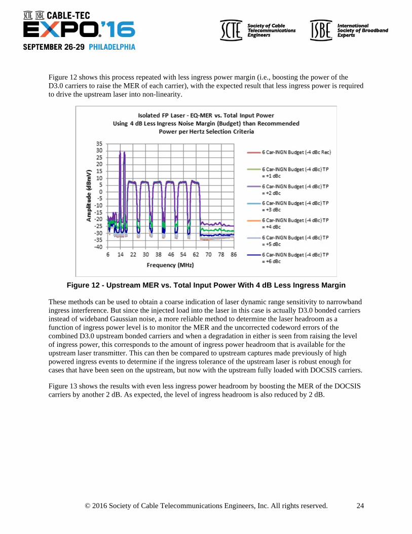
Figure 12 shows this process repeated with less ingress power margin (i.e., boosting the power of the D3.0 carriers to raise the MER of each carrier), with the expected result that less ingress power is required to drive the upstream laser into non-linearity.
Figure 12 - Upstream MER vs. Total Input Power With 4 dB Less Ingress Margin
These methods can be used to obtain a coarse indication of laser dynamic range sensitivity to narrowband ingress interference. But since the injected load into the laser in this case is actually D3.0 bonded carriers instead of wideband Gaussian noise, a more reliable method to determine the laser headroom as a function of ingress power level is to monitor the MER and the uncorrected codeword errors of the combined D3.0 upstream bonded carriers and when a degradation in either is seen from raising the level of ingress power, this corresponds to the amount of ingress power headroom that is available for the upstream laser transmitter. This can then be compared to upstream captures made previously of high powered ingress events to determine if the ingress tolerance of the upstream laser is robust enough for cases that have been seen on the upstream, but now with the upstream fully loaded with DOCSIS carriers.
Figure 13 shows the results with even less ingress power headroom by boosting the MER of the DOCSIS carriers by another 2 dB. As expected, the level of ingress headroom is also reduced by 2 dB.

© 2016 Society of Cable Telecommunications Engineers, Inc. All rights reserved. 25
Figure 13 - Upstream MER vs. Total Input Power With 6 dB Less Ingress Margin
Figure 14and Figure 15 are samples of interference seen in historical captures to make the point that the interference (narrowband ingress plus transient impulse/burst noise) can drive the upstream laser into nonlinearity.
Figure 14 – Upstream Interference Noise, Example 1
© 2016 Society of Cable Telecommunications Engineers, Inc. All rights reserved. 26
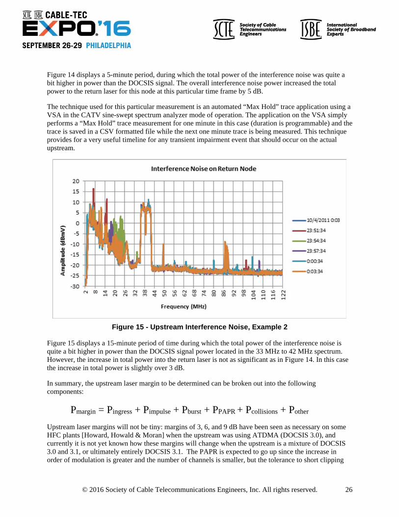
Figure 14 displays a 5-minute period, during which the total power of the interference noise was quite a bit higher in power than the DOCSIS signal. The overall interference noise power increased the total power to the return laser for this node at this particular time frame by 5 dB.
The technique used for this particular measurement is an automated “Max Hold” trace application using a VSA in the CATV sine-swept spectrum analyzer mode of operation. The application on the VSA simply performs a “Max Hold” trace measurement for one minute in this case (duration is programmable) and the trace is saved in a CSV formatted file while the next one minute trace is being measured. This technique provides for a very useful timeline for any transient impairment event that should occur on the actual upstream.
Figure 15 - Upstream Interference Noise, Example 2
Figure 15 displays a 15-minute period of time during which the total power of the interference noise is quite a bit higher in power than the DOCSIS signal power located in the 33 MHz to 42 MHz spectrum. However, the increase in total power into the return laser is not as significant as in Figure 14. In this case the increase in total power is slightly over 3 dB.
In summary, the upstream laser margin to be determined can be broken out into the following components:
Pmargin = Pingress + Pimpulse + Pburst + PPAPR + Pcollisions + Pother
Upstream laser margins will not be tiny: margins of 3, 6, and 9 dB have been seen as necessary on some HFC plants [Howard, Howald & Moran] when the upstream was using ATDMA (DOCSIS 3.0), and currently it is not yet known how these margins will change when the upstream is a mixture of DOCSIS 3.0 and 3.1, or ultimately entirely DOCSIS 3.1. The PAPR is expected to go up since the increase in order of modulation is greater and the number of channels is smaller, but the tolerance to short clipping

© 2016 Society of Cable Telecommunications Engineers, Inc. All rights reserved. 27
events should be greater due to the longer symbol durations of DOCSIS 3.1 OFDMA and improved error correction capability. It is recommended to explore this issue further in subsequent versions of this document.
As the power margins are increased, the maximum order of modulation and/or number of carriers possible on the upstream will correspondingly decrease for the older laser technology, thereby lowering the total capacity achievable on the network. Further, new sources of upstream interference such as HomePlugAV and HPNA have already been seen on the cable upstream, and their use is increasing. HomePlug AV2 extends the upper frequency range of the power line OFDM waveform from 30 MHz to 86 MHz, which would effectively cover the entire upstream even if expanded to 85 MHz. Therefore, characterizing the amount of laser margin required as the upstream is fully loaded is of paramount importance, as is an aggressive program to eliminate the source of such impairments on the upstream.
Upstream laser clipping can be clearly identified on analog upstream links by looking for any significant energy at frequencies above the highest active upstream frequency. This is clearly shown in Figure 16, where the green line shows a flat laser noise floor with no clipping and the blue trace shows strong laser clipping. In an HFC network using a digital return upstream optical link there may be a nominal amount of energy at frequencies above the highest active upstream frequency even when there is no clipping distortion taking place, so the key would be to look for energy in this part of the spectrum that is significantly above the nominal amount.
Figure 16 – Upstream Laser Clipping Due To Impulse Noise
6.4.4. Plant Sweeps
It is now possible using PNM technology to perform many aspects of plant sweeps using RF spectrum capture functionality. While early versions of PNM provided only amplitude vs. frequency characteristics, which is quite useful for detecting amplitude ripple, excessive tilt, adjacency issues, resonant peaking, LTE ingress, FM radio ingress, suckout, and rolloff and filter issues, see for example [SCTE PNM], D3.1
© 2016 Society of Cable Telecommunications Engineers, Inc. All rights reserved. 28
PNM promises full complex spectrum characterization, which would obviate the need for traditional unmodulated carrier-based sweep measurements.
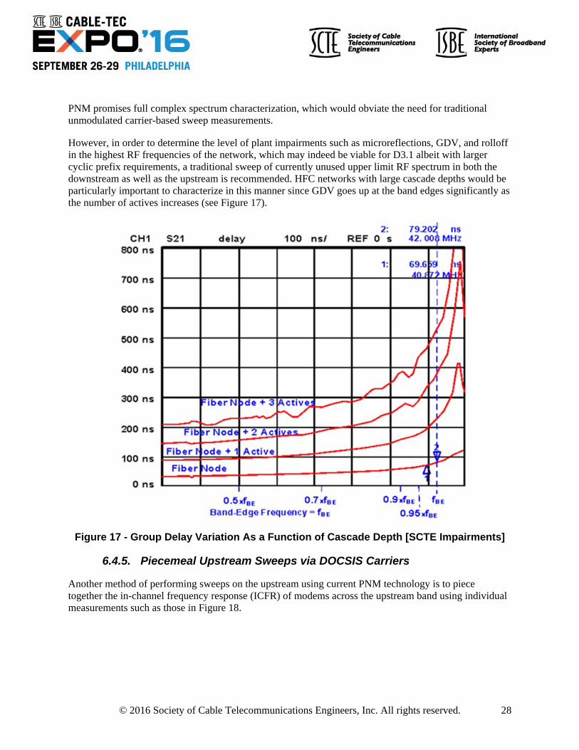
However, in order to determine the level of plant impairments such as microreflections, GDV, and rolloff in the highest RF frequencies of the network, which may indeed be viable for D3.1 albeit with larger cyclic prefix requirements, a traditional sweep of currently unused upper limit RF spectrum in both the downstream as well as the upstream is recommended. HFC networks with large cascade depths would be particularly important to characterize in this manner since GDV goes up at the band edges significantly as the number of actives increases (see Figure 17).
Figure 17 - Group Delay Variation As a Function of Cascade Depth [SCTE Impairments]
6.4.5. Piecemeal Upstream Sweeps via DOCSIS Carriers
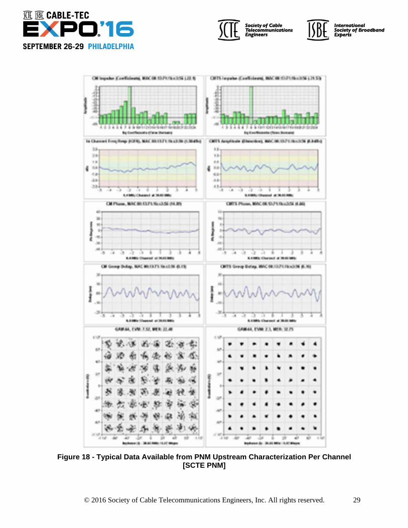
Another method of performing sweeps on the upstream using current PNM technology is to piece together the in-channel frequency response (ICFR) of modems across the upstream band using individual measurements such as those in Figure 18.
© 2016 Society of Cable Telecommunications Engineers, Inc. All rights reserved. 29
Figure 18 - Typical Data Available from PNM Upstream Characterization Per Channel [SCTE PNM]
© 2016 Society of Cable Telecommunications Engineers, Inc. All rights reserved. 30
6.4.6. Intermodulation Distortion Characterization via Unmodulated Carriers
Nonlinear distortion may appear to be decreasing as HFC networks become all-digital, but in actuality, the nonlinear distortion has been converted from narrowband carriers such as seen by CTB, CSO, and common path distortion (CPD) measurements, into a broadband overall noise floor. NPR measurement will be the most viable method of characterizing this composite intermodulation distortion, and this is now a feature of D3.1 PNM technology.
However, it is also possible to measure nonlinear distortion in the traditional way using injected carriers. The SCTE has planned two new updates to existing procedures since it has been shown that they can now be done in the field as well as in the lab [CableLabs PNM guideline update doc]. First, to characterize CPD there are a variety of test and monitoring equipment manufacturers that have novel and proprietary methods. It has also been shown in [CableLabs PNM] that by injecting an additional carrier into the downstream that is about 40 MHz offset from an existing leakage monitoring carrier found in many HFC networks (that does not interfere with existing signals), that the 40 MHz difference frequency CPD tone can be seen via upstream captures, thereby replicating the SCTE 109 2010 [SCTE 109] procedure for CPD characterization. 40 MHz was used since that frequency was unused and clean of interference, but other upstream frequencies could also be used to set the offset between the existing downstream leakage monitoring carrier and the additionally injected carrier for CPD measurement.
Second, the SCTE/ISBE plans to update SCTE 115 2011 [SCTE 115] for intermodulation distortion characterization using two carriers that proposes to use multiple carriers in advance of the ability to generate multiple, unmodulated carriers using D3.1. A separate operational practice for implementing this intermodulation distortion measurement is planned.
6.4.7. Transient Noise Characterization
A separate operational practice is in development for characterizing transient noise on the upstream, which includes both procedures using traditional equipment such as SAs, DSOs and VSAs, but also includes new ways to characterize transient impairments using D3.1 PNM features, including e.g. impulse noise statistics.
6.4.8. Leakage Characterization at Planned D3.1 Frequencies
SCTE/ISBE has released several recent operational practices on modern leakage prevention, detection, and mitigation practices, in particular covering measuring leakage in the UHF band in addition to traditional VHF band techniques [Hranac].
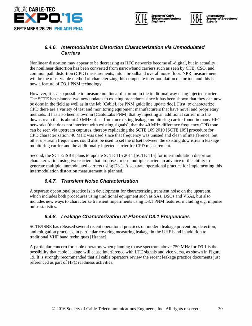
A particular concern for cable operators when planning to use spectrum above 750 MHz for D3.1 is the possibility that cable leakage will cause interference with LTE signals and vice versa, as shown in Figure 19. It is strongly recommended that all cable operators review the recent leakage practice documents just referenced as part of HFC readiness activities.
© 2016 Society of Cable Telecommunications Engineers, Inc. All rights reserved. 31
Figure 19 - Example Spectrum Capture From CM Showing Direct Pickup of LTE Signal
6.4.9. Phase Noise via High Order QAM Constellation Analysis and Carrier Injection with PNM
As the order of modulation increases, sensitivity to system phase noise increases. There are already procedures for measuring phase noise using injected carriers [SMRP Phase Noise] that use conventional test equipment. However, there are two approaches for monitoring phase noise that are now possible with PNM technology.
First, the signal QAM constellation can be captured and the usual azimuthal smearing of phase noise seen on the outermost constellation points will be an indication of phase noise issues. One way to enhance this measurement would be to use D3.1 modems transmitting at the highest possible order of modulation, even if the error rate is higher than typically desired for normal operation, in order to amplify the effects of phase noise on the constellation.
Second, there are often narrowband carriers injected into the downstream, and unmodulated carriers can also be injected on the upstream from a test point in the outside plant or in a friendly home, that could be captured using PNM RF spectrum capture at the highest possible resolution and the resulting spectrum compared to the spectrum of the carrier prior to passing through the HFC network that is captured either at the headend where the leakage monitoring carrier is injected (for downstream phase noise) or from the signal generator used for upstream phase noise. Viability of using PNM for phase noise measurement will depend on the minimum effective resolution bandwidth of the RF spectrum capture, and has yet to be tested in the field as of this writing.
6.4.10. Peak to Average Power Ratio (PAPR)
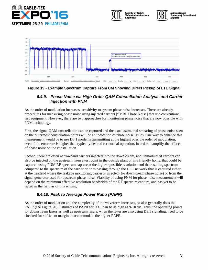
As the order of modulation and the complexity of the waveform increases, so also generally does the PAPR (see Figure 20). Estimates of PAPR for D3.1 can be as high as 9-10 dB. Thus, the operating points for downstream lasers as well as upstream lasers, when the latter are also using D3.1 signaling, need to be checked for sufficient margin to accommodate the higher PAPR.
© 2016 Society of Cable Telecommunications Engineers, Inc. All rights reserved. 32
Figure 20 - PAPR As a Function of OFDM Subcarriers [Wambach])
However, due to the large number of carriers and use of 256 QAM on the downstream, the PAPR for the existing downstream is likely already close to that of a Gaussian broadband signal, which means about 15 dB [SMRP PAPR]. Thus adding D3.1 signals is not expected to significantly affect PAPR on the downstream.
The upstream is another matter. As seen in the section on peak voltage addition in [SMRP], a small number of carriers that use lower orders of modulation such as is currently common on the upstream have a much lower PAPR, and thus could see a measurable increase in the PAPR when the upstream is fully loaded with D3.1 signals using higher order modulation.
Most modern DSOs and VSAs can measure PAPR for the upstream frequency band, and it is recommended to perform this measurement both in a clean laboratory HFC network (to determine the PAPR of the signals alone) and also for actual upstream signals in live plants (to determine the additional PAPR due to interference). A PAPR measurement using current upstream signals should be measured and compared to one using either additional D3.0 carriers to emulate a fully loaded plant, or ideally using all D3.1 OFDMA signals over the entire band of the upstream to determine the change in PAPR and thus the additional laser margin required on the upstream when converting all signals to D3.1 and fully loading the upstream.
© 2016 Society of Cable Telecommunications Engineers, Inc. All rights reserved. 33
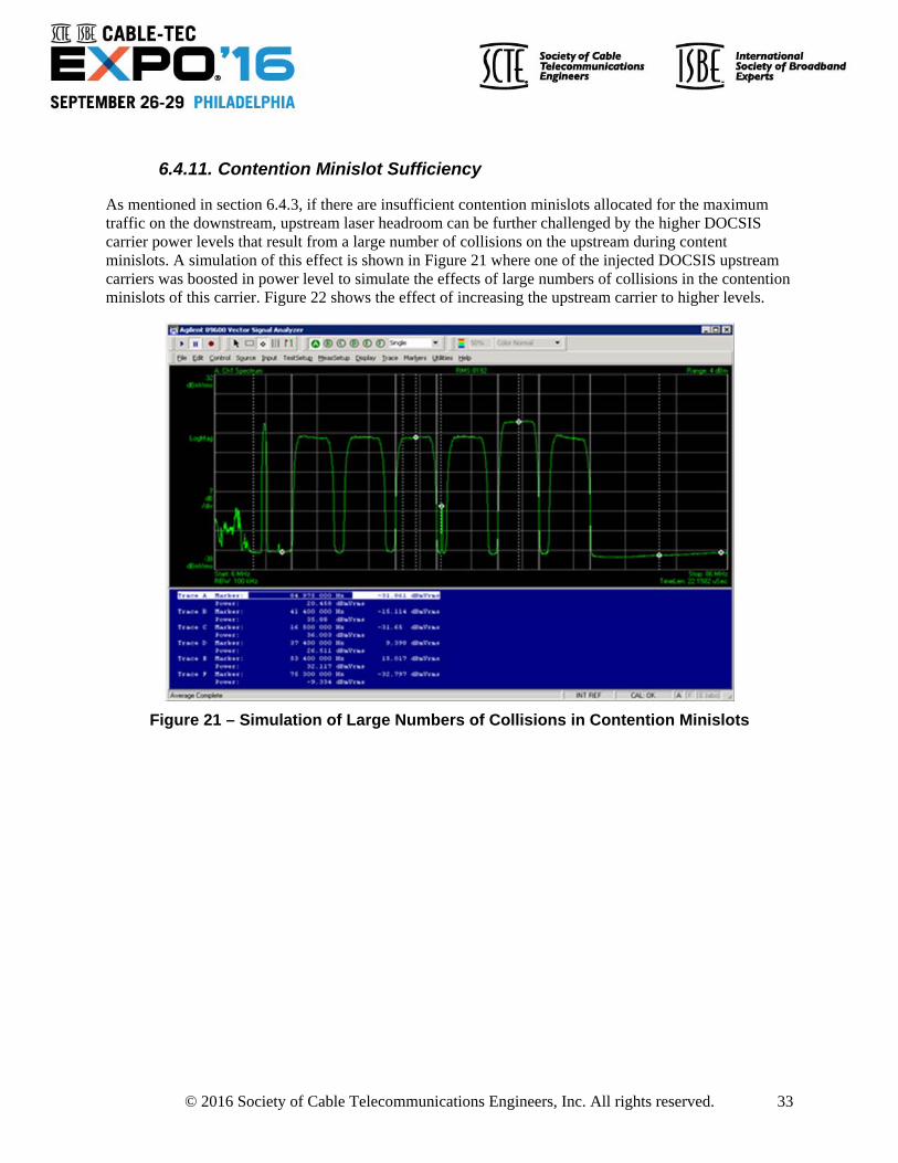
6.4.11. Contention Minislot Sufficiency
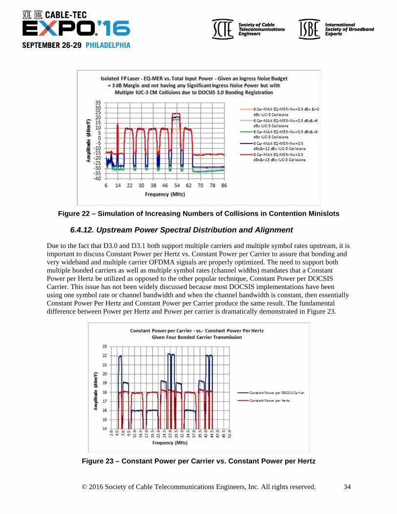
As mentioned in section 6.4.3, if there are insufficient contention minislots allocated for the maximum traffic on the downstream, upstream laser headroom can be further challenged by the higher DOCSIS carrier power levels that result from a large number of collisions on the upstream during content minislots. A simulation of this effect is shown in Figure 21 where one of the injected DOCSIS upstream carriers was boosted in power level to simulate the effects of large numbers of collisions in the contention minislots of this carrier. Figure 22 shows the effect of increasing the upstream carrier to higher levels.
Figure 21 – Simulation of Large Numbers of Collisions in Contention Minislots
© 2016 Society of Cable Telecommunications Engineers, Inc. All rights reserved. 34
Figure 22 – Simulation of Increasing Numbers of Collisions in Contention Minislots
6.4.12. Upstream Power Spectral Distribution and Alignment
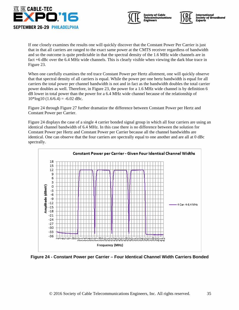
Due to the fact that D3.0 and D3.1 both support multiple carriers and multiple symbol rates upstream, it is important to discuss Constant Power per Hertz vs. Constant Power per Carrier to assure that bonding and very wideband and multiple carrier OFDMA signals are properly optimized. The need to support both multiple bonded carriers as well as multiple symbol rates (channel widths) mandates that a Constant Power per Hertz be utilized as opposed to the other popular technique, Constant Power per DOCSIS Carrier. This issue has not been widely discussed because most DOCSIS implementations have been using one symbol rate or channel bandwidth and when the channel bandwidth is constant, then essentially Constant Power Per Hertz and Constant Power per Carrier produce the same result. The fundamental difference between Power per Hertz and Power per carrier is dramatically demonstrated in Figure 23.
Figure 23 – Constant Power per Carrier vs. Constant Power per Hertz
© 2016 Society of Cable Telecommunications Engineers, Inc. All rights reserved. 35
If one closely examines the results one will quickly discover that the Constant Power Per Carrier is just that in that all carriers are ranged to the exact same power at the CMTS receiver regardless of bandwidth and so the outcome is quite predictable in that the spectral density of the 1.6 MHz wide channels are in fact +6 dBc over the 6.4 MHz wide channels. This is clearly visible when viewing the dark blue trace in Figure 23.
When one carefully examines the red trace Constant Power per Hertz allotment, one will quickly observe that that spectral density of all carriers is equal. While the power per one hertz bandwidth is equal for all carriers the total power per channel bandwidth is not and in fact as the bandwidth doubles the total carrier power doubles as well. Therefore, in Figure 23, the power for a 1.6 MHz wide channel is by definition 6 dB lower in total power than the power for a 6.4 MHz wide channel because of the relationship of 10*log10 (1.6/6.4) = -6.02 dBc.
Figure 24 through Figure 27 further dramatize the difference between Constant Power per Hertz and Constant Power per Carrier.
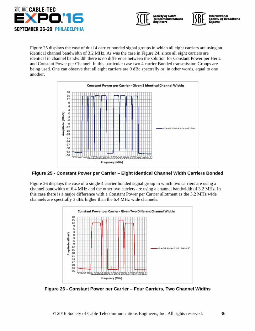
Figure 24 displays the case of a single 4 carrier bonded signal group in which all four carriers are using an identical channel bandwidth of 6.4 MHz. In this case there is no difference between the solution for Constant Power per Hertz and Constant Power per Carrier because all the channel bandwidths are identical. One can observe that the four carriers are spectrally equal to one another and are all at 0 dBc spectrally.
Figure 24 - Constant Power per Carrier – Four Identical Channel Width Carriers Bonded
© 2016 Society of Cable Telecommunications Engineers, Inc. All rights reserved. 36
Figure 25 displays the case of dual 4 carrier bonded signal groups in which all eight carriers are using an identical channel bandwidth of 3.2 MHz. As was the case in Figure 24, since all eight carriers are identical in channel bandwidth there is no difference between the solution for Constant Power per Hertz and Constant Power per Channel. In this particular case two 4 carrier Bonded transmission Groups are being used. One can observe that all eight carriers are 0 dBc spectrally or, in other words, equal to one another.
Figure 25 - Constant Power per Carrier – Eight Identical Channel Width Carriers Bonded
Figure 26 displays the case of a single 4 carrier bonded signal group in which two carriers are using a channel bandwidth of 6.4 MHz and the other two carriers are using a channel bandwidth of 3.2 MHz. In this case there is a major difference with a Constant Power per Carrier allotment as the 3.2 MHz wide channels are spectrally 3 dBc higher than the 6.4 MHz wide channels.
Figure 26 - Constant Power per Carrier – Four Carriers, Two Channel Widths
© 2016 Society of Cable Telecommunications Engineers, Inc. All rights reserved. 37
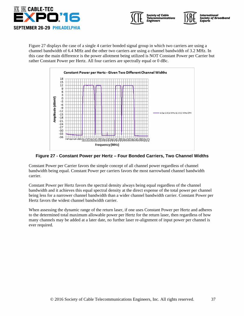
Figure 27 displays the case of a single 4 carrier bonded signal group in which two carriers are using a channel bandwidth of 6.4 MHz and the other two carriers are using a channel bandwidth of 3.2 MHz. In this case the main difference is the power allotment being utilized is NOT Constant Power per Carrier but rather Constant Power per Hertz. All four carriers are spectrally equal or 0 dBc.
Figure 27 - Constant Power per Hertz – Four Bonded Carriers, Two Channel Widths
Constant Power per Carrier favors the simple concept of all channel power regardless of channel bandwidth being equal. Constant Power per carriers favors the most narrowband channel bandwidth carrier.
Constant Power per Hertz favors the spectral density always being equal regardless of the channel bandwidth and it achieves this equal spectral density at the direct expense of the total power per channel being less for a narrower channel bandwidth than a wider channel bandwidth carrier. Constant Power per Hertz favors the widest channel bandwidth carrier.
When assessing the dynamic range of the return laser, if one uses Constant Power per Hertz and adheres to the determined total maximum allowable power per Hertz for the return laser, then regardless of how many channels may be added at a later date, no further laser re-alignment of input power per channel is ever required.
© 2016 Society of Cable Telecommunications Engineers, Inc. All rights reserved. 38
7. Coexistence of DOCSIS 3.1 and MoCA in the Home Environment
DOCSIS 3.1 and MoCA signals can both exist at frequencies above 1 GHz. The SCTE/ISBE has been working with MoCA representatives to create an operational practice [SWG MoCA] that explains how operators can use frequencies above 1 GHz for both types of services. The operational practice applies to any network that contains DOCSIS downstream signals at frequencies greater than 1 GHz and has MoCA signals in the premises. The calculations are valid for DOCSIS 3.1 and for MoCA 1.1 and 2.0 single channel operation. The three cases of how these signals may coexist are:
• Overlapping • Adjacent • Non-overlapping
The document provides many recommendations for operational best practices for the coexistence between DOCSIS 3.1 and MoCA. It explains the need for sufficient isolation and suggests the proper location and required performance of filters. Filters are necessary in most architectures to:
• Prevent MoCA signals from one residence from bridging to a nearby residence • Prevent overload of DOCSIS and MoCA receivers
Filter locations can be at the CPE and/or at the point of entry (PoE).
Home run vs. loop-through architectures are explained, with the final recommendation that non-overlapping channels and home run architectures be used whenever possible.
The recommendations are designed to assure that the DOCSIS and MoCA networks perform with minimal impact on each other. If the recommendations are not followed, significant performance degradation could occur to either network and, in some scenarios, one or both networks could completely fail to operate.
Conclusion The large number of HFC readiness activities possible could expand to overtake normal operations, if not prioritized properly. Thus the most important initial step is to look at all of the possible activities of interest to a given cable operator and rank them in terms of impact and benefit. In this manner, cable operators can focus their resources initially on the most important issues to resolve in preparing for a successful DOCSIS 3.1 deployment, and stage the remaining activities over a longer timeframe.
Appendix A: Comparison of DOCSIS 3.1 to 3.0 There are significant differences between DOCSIS 3.1 and 3.0, including specifically those at the physical, media access control, network layers of the open systems interconnect model, but other changes as well. A full comparison of the DOCSIS 3.1 specifications to those of 3.0 is beyond the scope of this document. However since part of HFC readiness involves training technicians, this appendix contains an initial description of key differences between the two specifications that would be most notable to technicians. As this document evolves in the SCTE special working group, this appendix will expand and perhaps become a separate document for training professionals in the cable industry.
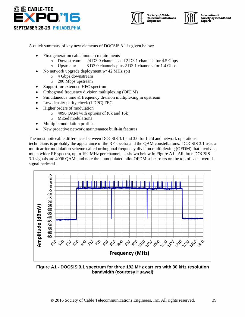
© 2016 Society of Cable Telecommunications Engineers, Inc. All rights reserved. 39
A quick summary of key new elements of DOCSIS 3.1 is given below:
First generation cable modem requirements o Downstream: 24 D3.0 channels and 2 D3.1 channels for 4.5 Gbps o Upstream: 8 D3.0 channels plus 2 D3.1 channels for 1.4 Gbps
No network upgrade deployment w/ 42 MHz spit o 4 Gbps downstream o 200 Mbps upstream
Support for extended HFC spectrum Orthogonal frequency division multiplexing (OFDM) Simultaneous time & frequency division multiplexing in upstream Low density parity check (LDPC) FEC Higher orders of modulation
o 4096 QAM with options of (8k and 16k) o Mixed modulations
Multiple modulation profiles New proactive network maintenance built-in features
The most noticeable differences between DOCSIS 3.1 and 3.0 for field and network operations technicians is probably the appearance of the RF spectra and the QAM constellations. DOCSIS 3.1 uses a multicarrier modulation scheme called orthogonal frequency division multiplexing (OFDM) that involves much wider RF spectra, up to 192 MHz per channel, as shown below in Figure A1. All three DOCSIS 3.1 signals are 4096 QAM, and note the unmodulated pilot OFDM subcarriers on the top of each overall signal pedestal.
Figure A1 - DOCSIS 3.1 spectrum for three 192 MHz carriers with 30 kHz resolution bandwidth (courtesy Huawei)
‐65‐60‐55‐50‐45‐40‐35‐30‐25‐20‐15‐10‐505
1015
Amplitude (dBmV)
Frequency (MHz)
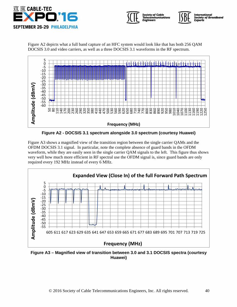
© 2016 Society of Cable Telecommunications Engineers, Inc. All rights reserved. 40
Figure A2 depicts what a full band capture of an HFC system would look like that has both 256 QAM DOCSIS 3.0 and video carriers, as well as a three DOCSIS 3.1 waveforms in the RF spectrum.
Figure A2 - DOCSIS 3.1 spectrum alongside 3.0 spectrum (courtesy Huawei)
Figure A3 shows a magnified view of the transition region between the single carrier QAMs and the OFDM DOCSIS 3.1 signal. In particular, note the complete absence of guard bands in the OFDM waveform, while they are easily seen in the single carrier QAM signals to the left. This figure thus shows very well how much more efficient in RF spectral use the OFDM signal is, since guard bands are only required every 192 MHz instead of every 6 MHz.
Figure A3 – Magnified view of transition between 3.0 and 3.1 DOCSIS spectra (courtesy Huawei)
‐60‐55‐50‐45‐40‐35‐30‐25‐20‐15‐10‐505
50
80
110
140
170
200
230
260
290
320
350
380
410
440
470
500
530
560
590
620
650
680
710
740
770
800
830
860
890
920
950
980
1010
1040
1070
1100
1130
1160
1190
1220
1250
Amplitude (dBmV)
Frequency (MHz)
‐55‐50‐45‐40‐35‐30‐25‐20‐15‐10‐505
605 611 617 623 629 635 641 647 653 659 665 671 677 683 689 695 701 707 713 719 725
Amplitude (dBmV)
Frequency (MHz)
Expanded View (Close In) of the full Forward Path Spectrum
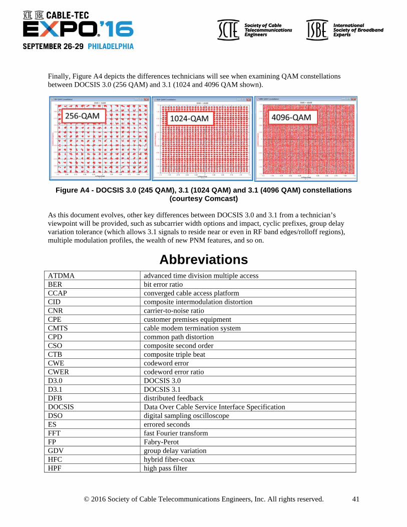
© 2016 Society of Cable Telecommunications Engineers, Inc. All rights reserved. 41
Finally, Figure A4 depicts the differences technicians will see when examining QAM constellations between DOCSIS 3.0 (256 QAM) and 3.1 (1024 and 4096 QAM shown).
Figure A4 - DOCSIS 3.0 (245 QAM), 3.1 (1024 QAM) and 3.1 (4096 QAM) constellations (courtesy Comcast)
As this document evolves, other key differences between DOCSIS 3.0 and 3.1 from a technician’s viewpoint will be provided, such as subcarrier width options and impact, cyclic prefixes, group delay variation tolerance (which allows 3.1 signals to reside near or even in RF band edges/rolloff regions), multiple modulation profiles, the wealth of new PNM features, and so on.
Abbreviations ATDMA advanced time division multiple access BER bit error ratio CCAP converged cable access platform CID composite intermodulation distortion CNR carrier-to-noise ratio CPE customer premises equipment CMTS cable modem termination system CPD common path distortion CSO composite second order CTB composite triple beat CWE codeword error CWER codeword error ratio D3.0 DOCSIS 3.0 D3.1 DOCSIS 3.1 DFB distributed feedback DOCSIS Data Over Cable Service Interface Specification DSO digital sampling oscilloscope ES errored seconds FFT fast Fourier transform FP Fabry-Perot GDV group delay variation HFC hybrid fiber-coax HPF high pass filter

© 2016 Society of Cable Telecommunications Engineers, Inc. All rights reserved. 42
ICFR in-channel frequency response ISBE International Society of Broadband Experts KPI key performance indicator MER modulation error ratio MoCA Multimedia over Coax Alliance MTR main tap ratio MTTR mean time to repair NPR noise power ratio OFDM orthogonal frequency division multiplexing OFDMA orthogonal frequency-division multiple access PAPR peak to average rower ratio PNM proactive network maintenance POE point of entry QAM quadrature amplitude modulation RFoG RF over Glass SA spectrum analyzer SCTE Society of Cable Telecommunications Engineers SES severely errored seconds VSA vector signal analyzer
Bibliography & References [CAB] “Midsplit Migration Implications on the HFC Network Technical Report,” CM-TR-MID-SPLIT-V01-150223, available from www.cablelabs.com, 2015.
[Moran1] J. Moran, “How to increase the upstream spectrum,” SCTE Cable-Tec Expo 2014 paper and presentation, available from www.scte.org, September, 2014.
[Thompson] R. Thompson, “What Home LAN Dreams May Come,” SCTE Cable-Tec Expo 2016 paper and presentation, Philadelphia, PA 2016, September 2016, available from www.scte.org
[Currivan & Wolcott] B. Currivan and L. Wolcott, “Leveraging DOCSIS 3.1 PNM measurements for plant performance optimization,” SCTE Cable-Tec Expo 2015 paper and presentation, New Orleans, LA, October 2015, available from www.SCTE.org.
[SCTE 174] SCTE 174 210, “Radio Frequency over Glass Fiber-to-the-Home Specification,” available from www.scte.org
[Benivedes] H. Benavides O., “Upgrade to 1 GHz networks,” SCTE Cable-Tec Expo 2014, International Breakfast presentation, Denver CO, September 2014, available from www.SCTE.org.
[SCTE Impairments] “Signal Impairments Recommended Practices,” Module in SCTE Broadband Distribution Specialist training course, available from www.SCTE.org.
[Hranac] S. Windle, R. Hranac, N. Segura, K. Couch, M. Darragh, G. Tresness and D. Howard “Operational practices for minimizing signal leakage in the UHF spectrum,” SCTE Journal of Network Operations volume 1, number 1, p. 55, January 2016.

© 2016 Society of Cable Telecommunications Engineers, Inc. All rights reserved. 43
[Moran2] J. Moran, “A new class of proactive network maintenance (PNM) measurements and tools,” SCTE Cable-Tec Expo 2015 paper and presentation, New Orleans, LA, October 2015, available from www.SCTE.org.
[Howard] D. Howard, “Detection and classification of RF impairments for higher capacity upstreams using advanced TDMA,” NCTA Spring Technical Forum proceedings, available from www.nctatechnicalpapers.com.
[SMRP NPR] “Noise Power Ratio (PNR),” page 190, in SCTE Measurement Recommended Practices For Cable Systems, 4th ed., 2012, available from www.SCTE.org.
[SMRP Peak-Avg] “Peak-to-Average Ratio,” page 31, in SCTE Measurement Recommended Practices For Cable Systems, 4th ed., 2012, available from www.SCTE.org.
[Howard, Howald & Moran] D. Howard, R. Howald, and J. Moran, “HFC readiness for DOCSIS 3.1,” presented at SIT March 2014 to Cablevisión Argentina, and also found in [SCTE Signal Impairments Module] reference above.
[Howald] R. Howald, P. Chang, R. Thompson, D. Stoneback, V. Rathod, C. Moore, “Characterizing and Aligning the HFC Return Path for Successful DOCSIS 3.0 Rollouts,” SCTE Cable-Tec Expo 2009 paper and presentation, Denver, CO, October 2009, available from www.SCTE.org.
[Hunter] D. Hunter, “Improved customer service through intermittent detection,” SCTE Cable-Tec Expo 2015 paper and presentation, New Orleans, LA, October 2015, available from www.SCTE.org.
[Urban] D. Urban MER histogram, found in many DOCSIS 3.1 white papers and presentations. See for example T. Cloonan and M. Emmendorfer, “Examining the future evolution of the access network,” available from www.arris.com, or R. Howald, J. Moran and D. Howard “DOCSIS 3.1 HFC readiness special working group update,” presentation at DOCSIS 3.1 Engineering Symposium, SCTE Cable-Tec Expo 2013, available from www.SCTE.org.
[Garcia] M. Garcia, “Device testing and evaluation of PNM test operations via signal analysis,” SCTE Cable-Tec Expo 2016 paper and presentation, Philadelphia, PA 2016, September 2016, available from www.scte.org
[SCTE 119] SCTE 119 2011, “Measurement Procedure for Noise Power Ratio,” available from www.scte.org
[SCTE PNM] Module 3, “Using PNM,” in Proactive Network Maintenance, SCTE online course, available from www.SCTE.org
[CableLabs PNM] “CPD Detection,” in Proactive Network Maintenance Using Pre-equalization, (draft revision, to be published in late 2016), available from www.cablelabs.com.
[SCTE 109] ANSI/SCTE 109 2010, “Test Procedure for Common Path Distortion (CPD),” available from www. scte.org
[SCTE 115] ANSI/SCTE 115 2011, “Test Method for Reverse Path (Upstream) Intermodulation Using Two Carriers,” available from www.scte.org

© 2016 Society of Cable Telecommunications Engineers, Inc. All rights reserved. 44
[SMRP Phase Noise] “Phase Noise,” page 51, in SCTE Measurement Recommended Practices For Cable Systems, 4th ed., 2012, available from www.SCTE.org
[Wambach] H. Wambach, “DOCSIS 3.1 benefits and HFC readiness,” SCTE Cable-Tec Expo 2015, International Breakfast presentation, New Orleans, LA, October 2015, available from www.SCTE.org.
[SMRP PAPR] “Peak Voltage Addition,” p. 249 in SCTE Measurement Recommended Practices For Cable Systems, 4th ed., 2012, available from www.SCTE.org
[SWG MoCA] “Operational Practice for the Coexistence of DOCSIS 3.1 and MoCA in the Home Environment,” HFCR001r5, preliminary draft, available from www.scte.org (must be member of SCTE Standards program), June 2016.