evaluating municipal water conservation policies using · pdf filewater resour manage (2010)...

Water Resour Manage (2010) 24:3371–3395DOI 10.1007/s11269-010-9611-2

Evaluating Municipal Water Conservation PoliciesUsing a Dynamic Simulation Model

Sajjad Ahmad · Dinesh Prashar

Received: 11 August 2009 / Accepted: 3 February 2010 /Published online: 17 February 2010© Springer Science+Business Media B.V. 2010

Abstract A dynamic simulation model is developed for South Florida to capture theinterrelationships between water availability and competing municipal, agricultural,and environmental water demands. This paper presents the model structure andfindings related to municipal water demand and potential for water conservation.The policies of introducing low flow appliances, xeriscaping, and pricing are testedfor their effectiveness in reducing municipal water demand. Performance criteria ofreliability, resilience, and vulnerability are used to measure the success of policies.Policies are also evaluated for their impact on environmental flow requirements. Themodel is calibrated using data from 1975 to 2005 for population growth, municipalwater demand, and water levels in Lake Okeechobee; and simulations are carriedout from 2005 to 2030 on a monthly time step. Sensitivity analysis is performed andextreme condition tests are conducted to evaluate the robustness of the model. Thestatus-quo (defined as no changes in the current water use patterns) simulations showa reduction in environmental flows after 2010 leading to an increase in the numberof minimum flow level violations. Policies tested show potential for a reduction inmunicipal demand and for improvement in environmental flows.

Keywords System dynamics · Water conservation · South Florida ·Municipal water demand · Pricing · Xeriscaping · Low flow appliances

1 Introduction

With rapidly growing populations, many regions in the world are finding it difficultto meet municipal, agricultural, and environmental water demands simultaneously.South Florida, located in the southeastern USA, is an example of such a region. At

S. Ahmad (B) · D. PrasharDepartment of Civil and Environmental Engineering, University of Nevada,Las Vegas, NV 89154-4015, USAe-mail: [email protected]

3372 S. Ahmad, D. Prashar

first glance, it would appear very unlikely for South Florida to face water shortages,since it experiences a sub-tropical climate and an average annual rainfall of 134 cm.However, several factors contribute towards the region’s distinct characteristic ofbeing water rich and yet not having enough freshwater resources. Seventy-threepercent, or 98 cm, of the region’s spatially averaged annual rainfall occurs in the sixmonth period from May through October (Ali and Abtew 1999). Rainfall in SouthFlorida has a high spatial and temporal variability and annual rainfall totals varybetween 112 cm and 168 cm (Alaa et al. 2000). Although water due to rainfall isrelatively abundant in Florida, a major portion of it is never available for use dueto high evapotranspiration rates. Measured runoff averages from 0 to 25 cm peryear in much of south Florida. The region overlies two major aquifer systems, theBiscayne and Floridian Aquifer Systems; and the main source of water supply inSouth Eastern Florida is the Biscayne Aquifer. It is classified as a sole source of watersupply by the US Environmental Protection Agency (EPA) and is highly susceptibleto contamination due to its permeability and shallow depth.

In Florida, water, both surface and ground, is managed by five water managementdistricts; the South Florida Water Management District (SFWMD) is the largestamong them managing nearly 49% of all freshwater withdrawals in the State. Itsjurisdiction covers a land area of 46,400 km2 and its population is expected togrow from 7.5 million in 2010 to 10.7 million by 2030 (USACE and SFWMD 1999;Florida Consensus Estimating Conference 2000). The Lower East Coast (LEC),which covers an area of 15,800 km2, is the most densely populated region in thestate with more than 5 million people. The municipal water demand alone in SouthFlorida in 2005 was 1,640 million cubic meters (Mm3) (1.33 million acre-feet [ac-ft]).Ninety six percent of this demand is primarily fulfilled from Biscayne Aquifer, whichunderlies the LEC.

In addition to municipal water demands, agriculture is another major waterconsumer in South Florida. The region’s favorable climate allows for a large numberof crops to be grown in all seasons. The major crops grown in South Florida includesugarcane, citrus, and other row crops. Total agricultural water demand in SouthFlorida in 2005 was 3,650 Mm3 (2.96 million ac-ft). Sixty two percent of agriculturalwater demand is met from ground water sources and the remaining 38% is met fromsurface water sources. Because of population increase and land use conversions thetotal agricultural area is likely to remain at the current level or decrease in the future.Therefore, no significant increase in agricultural water demand is expected. Most ofthe future growth in water demand will be in the municipal sector.

Figure 1 shows the physical features of South Florida. Lake Okeechobee, whichis also called the “liquid heart” of South Florida’s water supply and flood controlsystem, covers 1,792 km2 and is the biggest source of fresh surface water in the region.It has an average depth of 2.4 meters and maximum depth of less than 6 meters.Recharge of the lake comes from rainfall and from the Kissimmee River in the North.The lake has two outlets: the Caloosahatchee River to the West and the St. LucieCanal to the East, discharging to the Gulf of Mexico and the Atlantic Ocean,respectively. Four major canals (West Palm Beach, Hillsboro, North New River andMiami) are used to release water from the Lake to meet demands. The Lake hasa water storage capacity of over 4,624 Mm3. It provides irrigation water for the1,792 km2 Everglades Agriculture Area (EAA) and supplements the water supplyfor the Everglades National Park during dry periods (SFWMD 2002). Operation of

Evaluating Municipal Water Conservation Policies. . . 3373

Fig. 1 Study area: SouthFlorida Water ManagementDistrict (Source SFWMDwebsite)

the Lake has numerous environmental and economic consequences (Vedwan et al.2008).

South of the EAA, Water Conservation Areas (WCA) are located that coveran approximate area of 3,550 km2 and have a storage capacity of 2,344 Mm3

(1.9 million ac-ft). These surface water impoundments were developed to provideflood control, water storage, ground water recharge, and wildlife conservationbenefits for the region.

South Florida is also home to vital environmental resources that have significantwater demands. Everglades National Park is the largest subtropical wilderness in theUSA. The park contains temperate and tropical plant communities including saw-grass prairies, mangrove and cypress swamps, pinelands and hardwood hammocks,as well as marine and estuarine environments. Known for its abundant bird andwildlife, the park has large wading bird colonies of various species and is host torare and endangered wildlife, including the American crocodile, Florida panther,and West Indian manatee. Everglades National Park was the first national park tobe established to preserve biological resources—to protect the natural conditions ofthe subtropical Everglades ecosystem. The park is designated as an InternationalBiosphere Reserve, a World Heritage Site, and a Wetland of InternationalImportance, in recognition of its significance (Davis and Ogden 1994).

The 1997 Florida State Water Act required the Water Management Districts toset up minimum flow levels (MFLs) for all water bodies within their jurisdiction tomaintain the environmental resources and ecosystem functions of the region. These


minimum flows are maintained while managing the system in accordance with thelaws set by the Florida Legislature to protect the environment from ‘harm’, whichhas been defined in Florida administrative code as the temporary or permanent lossof water resource functions (FAC 2006). The act also requires the governing bodiesto undertake studies to assess the water availability for not less than 20 years in thefuture and make contingency plans wherever required.

This study draws inspiration from the Water Act and consumptive use permittingrequirements, and is focused on evaluating different policies for their potential toreduce municipal water demand and meet environmental flow requirements in SouthFlorida. Indoor water use can be reduced by using low flow appliances such as toilets,faucets, showers, and washers. Outdoor water use can be reduced by using nativeplants and water smart landscaping (i.e., xeriscaping). Water pricing has the potentialto reduce water demand both for outdoor and indoor use. We use a system dynamicsmodeling approach to develop a dynamic simulation model to evaluate these waterconservation policies over a time horizon of 25 years (2005–2030).

The remainder of the paper is organized as follows. First, a brief and selectivereview of system dynamics applications in water resources is presented. This isfollowed by the details of the dynamics model developed and data used. Modelresults are presented and discussed in the subsequent section. Finally, a summaryof the work is presented and conclusions are drawn.

2 System Dynamics

The system dynamics (SD) modeling approach is used in this study to developa dynamic simulation model. The underlying difference between SD and othermodeling approaches is the study of a system in terms of stocks and flows, whichaffect each other through feedback loops. Together, stocks and flows produce effectsand display system properties that cannot be attributed to any of the individualcomponents making up a system. A SD modeling approach can also capture timedelays and internal feedback loops that alter the behavior of the system (Sterman2000).

Over the years a number of studies on water resources planning and managementhave been conducted using SD. Winz et al. (2009) have discussed the theoreticaland practical evolution of SD in the area of water resources management over thepast 50 years. Some notable applications in water resources include Gao and Liu(1997) who developed a SD model for analysis of the regional water resources systemin Hanzhong Basin, China. Simonovic and Fahmy (1999) illustrated the use of SDin structuring water resources policy for the Nile River Basin in Egypt. Ahmadand Simonovic (2000) developed a SD model for reservoir operation and evaluatedthe capacity of a reservoir to handle large floods. Guo et al. (2001) developed aSD model for environmental planning and management in the Lake Erhai Basin,China. Xu et al. (2002) developed a SD model to evaluate the sustainability ofYellow River water resources in China. Stave (2003) developed a SD model tofacilitate stakeholder participation in water resources planning process in the LasVegas Valley in Nevada. Tidwell et al. (2004) developed a SD model to assist incommunity based planning for water resources in the Middle Rio-Grande Basin.Simonovic and Ahmad (2005) developed a SD model to simulate human behavior


during emergency evacuation orders for floods. Ahmad and Simonovic (2006) usedSD to develop a decision support system for management of floods. Chung et al.(2008) presented a SD based water supply planning model for urban settings.

Some SD models on a larger scale (i.e., country or world level) have also beendeveloped by Simonovic (2002), wherein the future development of world, based onWorld3 simulations, is used to estimate the stressors on water supply. An offshootof the same model, the CanadaWater model was developed to evaluate the waterresources of Canada (Simonovic and Rajasekaram 2004). SD has also found applica-tion in describing hydrological processes such as in Li and Simonovic (2002). Sayseland Barlas (2001) display the effects of salinization and water availability on regionalcrop yields. Ahmad and Simonovic (2004) introduced the idea of Spatial SystemDynamics by integrating SD with GIS to represent spatial processes. Elshorbagyet al. (2005) developed a SD model to assess the sustainability of reclamationof disturbed watersheds. Some recent studies using SD include management of ariver basin in Iran (Madani and Mariño 2009), water accounting system for watermanagement (Graham et al. 2009), a decision support system for water management(Jesús et al. 2009) and reservoir operation performance under climate change (Liet al. 2010).

Taking into account the large number of components, feedback mechanisms,behavioral responses and time lags in the system to be modeled, SD is considered tobe an appropriate tool for this study. The elements in the modeled system including:population growth, land use changes, water demand (municipal, agricultural, andenvironmental) and water availability (surface water and groundwater), are intercon-nected in several ways directly and indirectly. For example, urban population growthnecessitates the conversion of agricultural or natural land into urban land resultingin an increase in urban demand and a reduction in agricultural water consumption.Such connections may not be intuitively obvious to decision makers when policies arebeing formulated. In addition, behavioral response of municipal water consumers toprice changes is captured in the model. Thus helping the planners and managers toexplore hypothesis and evaluate the impacts of their decisions in avenues, which arenot directly connected to the point of intervention. The SD model developed forthis study, using the concepts of rainfall-runoff transformation and water balance,estimates water availability for the competing uses of municipal, agricultural, andenvironmental demands. Based on population growth and land use changes, themodel generates water demands for municipal, agricultural, and environmental use.Several policies to reduce municipal water demand are evaluated. The model alsoimproves the understanding of the internal workings of a complex hydrologicalsystem. The laws and the legislations, leading to the formulation of the district widewater management plans and MFLs, provide a framework within which this study isconducted. Details of the model are presented in the following section.

3 Model Structure

This paper is derived from a larger study, which evaluates the water conservationpotential of different policies aimed at agricultural and municipal water use inSouth Florida. The model structure and findings related to conservation in themunicipal water use are reported in this paper. The SD model is divided into eight


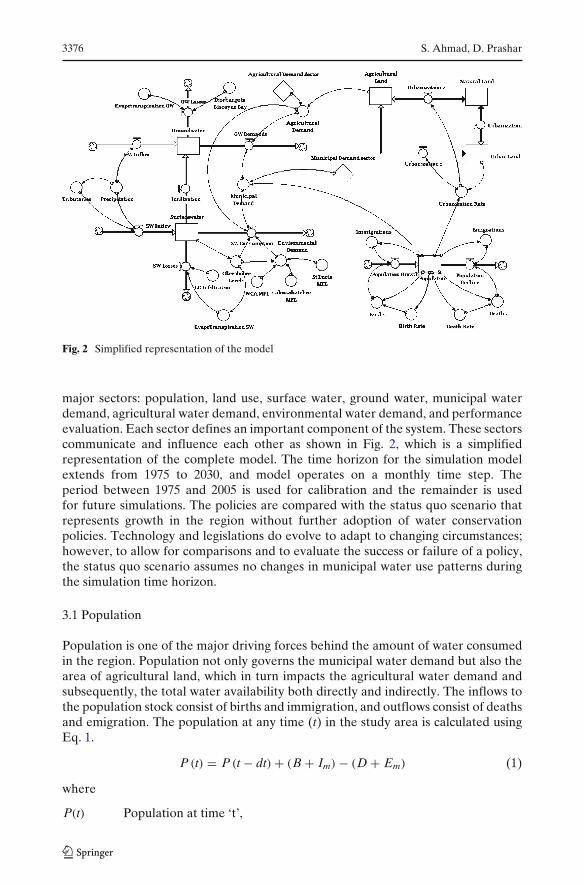
Fig. 2 Simplified representation of the model

major sectors: population, land use, surface water, ground water, municipal waterdemand, agricultural water demand, environmental water demand, and performanceevaluation. Each sector defines an important component of the system. These sectorscommunicate and influence each other as shown in Fig. 2, which is a simplifiedrepresentation of the complete model. The time horizon for the simulation modelextends from 1975 to 2030, and model operates on a monthly time step. Theperiod between 1975 and 2005 is used for calibration and the remainder is usedfor future simulations. The policies are compared with the status quo scenario thatrepresents growth in the region without further adoption of water conservationpolicies. Technology and legislations do evolve to adapt to changing circumstances;however, to allow for comparisons and to evaluate the success or failure of a policy,the status quo scenario assumes no changes in municipal water use patterns duringthe simulation time horizon.

3.1 Population

Population is one of the major driving forces behind the amount of water consumedin the region. Population not only governs the municipal water demand but also thearea of agricultural land, which in turn impacts the agricultural water demand andsubsequently, the total water availability both directly and indirectly. The inflows tothe population stock consist of births and immigration, and outflows consist of deathsand emigration. The population at any time (t) in the study area is calculated usingEq. 1.

P (t) = P (t − dt) + (B + Im) − (D + Em) (1)

where

P(t) Population at time ‘t’,


P(t− dt) Population at previous time step,B Number of births in time dt,Im Number of immigrations in time dt,D Number of deaths in time dt, andEm Number of emigrations in time dt.

The immigration rate, emigration rate, death rate, and birth rate are obtainedfrom a study on Florida’s population growth and demographics (Smith 2005). Theshift of populations within the district is assumed not to impact the overall water con-sumption, therefore, is not accounted for. Population growth in the model is trackedseparately for periods before and after 2010. This division helps in implementing thewater conservation policies that are introduced after 2010.

3.2 Land Use

Land use in the study area is divided into three categories: urban, agricultural, andnatural. Land use data is obtained from the GIS catalog of SFWMD land use and landcover maps (http://my.sfwmd.gov/gisapps/sfwmdxwebdc/). The land use coverage isavailable for 1988, 1995, 1999, and 2004. The distribution of land use in 1988 was59.1% natural, 29.5% agricultural, and 11.4% urban (USACE and SFWMD 1999),and changes to 57.8% natural, 27.7% agricultural, and 14.5% urban by 2005. Forthe simulation horizon, land use in the district is expected to undergo considerablechanges. These changes are capable of bringing about a significant increase in waterconsumption as well as the relative distribution of water demand among variouscompeting uses.

Land use changes are governed by several factors such as population growth,economy, and legislations. While it is not possible to include the impacts of un-foreseen changes in economy and legislations in the model, it is able to simulatethe changes arising due to population growth, agricultural policies, water use andwater availability. The transfers in the status quo scenario are assumed to be drivenby anticipated population growth, which result in land transfers from natural toagricultural, natural to urban, and agricultural to urban land uses. Beyond the statusquo scenario, the model allows testing of several policy options of shifting landuses and controlling the rates at which land use changes take place. For example,it is possible to evaluate the water savings if some agricultural land is set aside forconservation purposes and converted to natural land. The amount of agriculturalland in the study area at any time (t) is calculated using Eq. 2.

LAg (t) = LAg (t − dt) + (CAg

) − (Pgr × F

)(2)

where

LAg Agricultural land,CAg Conversion of natural land into agricultural land in time dt,Pgr Population growth in time interval dt, andF Urbanization factor in time interval dt.

Conversion from natural and agricultural to urban land uses is controlled bythe urbanization factor which takes into account the negative feedback betweenpopulation growth and dwindling land availability. The allocation rate decreasesas population density increases and less land is available for further conversion.

http://my.sfwmd.gov/gisapps/sfwmdxwebdc/


The rate of conversion is derived from a study conducted to determine the rate ofurbanization of Florida due to increasing population (Zwick and Carr 2006).

3.3 Surface Water

Lake Okeechobee is the primary stock in the surface water sector. The inflow intoLake Okeechobee comprises of rainfall occurring over the lake, and the runofffrom Kissimmee River basin. The outflows consist of evapotranspiration, and con-sumption that includes agricultural and municipal water demands, flood protectiondischarges, and environmental flows to St. Lucie, Caloosahatchee River, and WCAs.The amount of water in the lake at a time (t) is calculated using Eq. 3.

SW (t) = SW (t − dt) + Qin − (ET + Wd + ILO) (3)

where

SW(t) The volume of water contained in the lake at time t,Qin Inflow in the time interval dt,ET Evapotranspiration in the time interval dt,Wd Water demand in the time interval dt, andILO Infiltration from Lake Okeechobee in the time interval dt.

Monthly evapotranspiration estimates are used from a study conducted in SouthFlorida by Abtew et al. (2003). The water levels in Lake Okeechobee are maintainedthrough regulatory and non regulatory releases. The regulatory releases are madeaccording to a calendar based schedule, shown in Fig. 3 and Table 1, established byUS Army Corps of Engineers and SFWMD to ensure the peripheral integrity of thelevee constructed around the lake. The schedule is designed to have minimum impacton the ecology of the downstream systems and at the same time meeting the floodcontrol requirements. Non regulatory discharges are made in order to serve a varietyof purposes such as irrigation, municipal water supply, prevention of saltwater intru-sion, and maintenance of MFLs. Operating rules for Lake Okeechobee are defined

12

13

14

15

16

17

18

19

Jan Feb Mar Apr May Jun Jul Aug Sep Oct Nov Dec

Lake

Sta

ge (

ft a

bove

NG

VD

)

Zone A

Zone B

Zone E

Zone D

Zone C

Fig. 3 Lake Okeechobee water surface elevation regulation schedule


Table 1 Lake Okeechobee water surface elevation regulation schedule

Zone Flow to WCAs Caloosahatchee River St. Lucie Canal

A Max practicable Up to max capacity at S-77 Up to max capacity at S-80B Max practicable 184 m3/s (6,500 cfs) at S-77 100 m3/s (3,500 cfs) at S-80C Max practicable Up to 127 m3/s (4,500 cfs at S-77) Up to 70 m3/s (2,500 cfs) at S-80D Max practicable Max non-harmful discharge to Max non-harmful discharge to

estuary when stage rising estuary when stage risingE No regulatory No regulatory discharge No regulatory discharge

discharge

in the model using if-then-else statements using information from Fig. 2 and Table 1.Inflow to Lake Okeechobee is estimated from excess precipitation information avail-able at SFWMD GIS Data Catalogue (http://my.sfwmd.gov/gisapps/sfwmdxwebdc/)and Abtew et al. (2007).

3.4 Groundwater

In order to estimate the capacity of Biscayne Aquifer, it is idealized as a wedge withits thicker end towards the Atlantic Ocean. The average storage coefficient for theBiscayne Aquifer is approximately 0.2 (Klein and Hull 1978). The product of thevolume and storage coefficient gives the amount of water the aquifer can hold, whichis approximately 34,068 Mm3. The groundwater stock at a time (t) in the model iscalculated using Eq. 4.

GW (t) = GW (t − dt) + R − (Wd + GWL) (4)

where

GW(t) The volume of water contained in the aquifer at time (t),R Recharge in the time interval dt,Wd Water demand in the time interval (dt), andGWL Ground water losses in the time interval (dt).

The recharge primarily comes from percolation of precipitation, recharge fromagricultural water use, and the infiltration from the surface water bodies. Therecharge into the groundwater is obtained using Eq. 5.

R = (CI × P) + RAg + IWCA + ILO (5)

Where

CI Coefficient of infiltration,P Precipitation,RAg Recharge from agricultural water use, andIWCA Infiltration from WCAs

Recharge is estimated from recharge/discharge information available for SouthFlorida Water Management Model at SFWMD GIS Data Catalogue (http://my.sfwmd.gov/gisapps/sfwmdxwebdc/).

The outflows from Biscayne Aquifer consist of withdrawals for 62% of agricul-tural and 96% of municipal water requirements in the district. These withdrawals incombination with evapotranspiration and seepage into the Bay of Biscayne lead to





a significant amount of outflows from Biscayne Aquifer. The total outflows fromthe groundwater for status quo scenario are calculated using Eq. 6. For futuresimulations, the division of water withdrawals from surface and groundwater waskept flexible to explore different allocation options.

Wd = (0.96 × Mu) + (0.62 × Ag) + Env (6)

where

Mu Municipal demand,Ag Agricultural demand,Env Environmental demand.

GWL = ET + Qb (7)

Where

Qb discharge to Biscayne Bay.

Estimates of evapotranspirations from ground water and discharge to BiscayneBay were adopted from Parker et al. (1955).

3.5 Municipal Water Demand

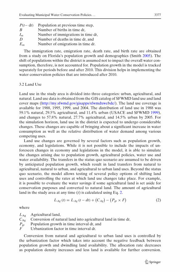
The average per capita per day water consumption of 658 l (174 gallons per personper day) is used as a base demand (SAFE 1995). The municipal water conservationpolicies are then implemented to estimate the potential water savings compared tothe base demand. Base demand includes municipal, industrial, and commercial wateruses. Sixty one percent of this demand is municipal use. Moreover, approximately70% of water in municipal use is used indoors and the rest is used outdoors for lawnirrigation (Marella 2000, 2008; Kaminski 2004). The water conservation in this studyonly focuses on municipal indoor and outdoor uses. Figure 4 shows components ofmunicipal water demand that are impacted by water conservation policies.

The municipal water use is split into indoor and outdoor uses and the indoorwater use is further divided into use in bath/showers, toilet, faucets, laundry, andleaks. The average distribution of indoor water use in the USA is as follows: shower19%, toilet 26%, faucet 16%, laundry 22%, leaks 14%, and others 3% (Mayer et al.1999). This division of indoor water use allows the implementation of low flowappliances separately for each water use. Different numbers have been reported inthe literature for conservation that can be achieved using low flow appliances. Ahousehold water conservation study estimated savings of up to 44% by using low flowappliances (Vickers 2001). However it is widely recognized that actual savings due tolow flow appliances are usually lower than rated because of the behavioral responseof consumers (Davis 2008; Mayer et al. 1999; Renwick and Green 2000). Such studiesuse intrusive data collection methods, which can lead to unreliable results. The savingfrom low flow appliances may not be fully realized if not used in conjunction withincrease in municipal water rates (Timmins 2003). This model incorporates the effectof the behavioral response of consumers by lowering the savings achieved by the lowflow appliances twenty percent below their rated efficiencies.


MunicipalDemand

Non-domesticSupply

DomesticSupply

OutdoorDomestic

IndoorDomestic

Kitchen

Laundry

Bath

Toilet

Leakages

PublicSupply

IndustrialSupply

CommercialSupply

Final MunicipalDemand

ModifiedDomestic

Interventions

Interventions

Fig. 4 Chart showing components of municipal water demand that are impacted by water conserva-tion policies

In addition to low flow appliances, raising the price of municipal water is alsotested for its potential in water conservation. Pricing has impacts on water con-sumption and it can enhance the conservation achieved using other methods suchas low flow appliances and xeriscaping. Therefore, it can be potentially used as anoption to reduce water consumption by itself or in conjunction with other methods.The relation between the price of a commodity and its consumption is called ‘priceelasticity’ (Renwick et al. 1998). Price elasticity for municipal water consumptionaccording to a number of studies varies from −0.15 to −0.52 depending upon the baseprice of water (Nieswiadomy 1992; Renwick et al. 1998; Olmstead et al. 2007). Sincewater is an essential commodity, a certain amount of water is required irrespectiveof the price, therefore, beyond a certain point, a further increase in pricing does notaffect consumption. For US customers, the price elasticity has been estimated to bearound −0.33 (Olmstead et al. 2007) and has been used in the model.

Approximately 30% of the municipal water is used for irrigation and otheroutdoor water uses (Kaminski 2004). Potential water conservation in outdoor useis evaluated by implementing pricing, xeriscaping or a combination of the two.Section 373.185, Florida Statutes, defines xeriscape or Florida friendly landscapeas “quality landscapes that conserve water and protect the environment and areadaptable to local conditions and which are drought tolerant. The principles ofxeriscape include planning and design, appropriate choices of plants, soil analysiswhich may include the use of solid waste compost, efficient irrigation, practical useof turf, appropriate uses of mulches and proper maintenance.” A number of studiesconducted on xeriscaping at different locations within the USA suggest that watersaving range between 25% and 42% (Nelson 1994; Testa and Newton 1993; Sovocool2005; Vickers 2006). In this study we use a conservative estimate of 30% reduction inoutdoor municipal water use when xeriscaping is implemented.


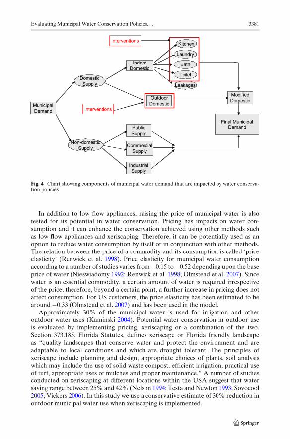
Table 2 Annualenvironmental water demands

Water body Minimum flow requirements

Lake Okeechobee Average three monthly waterlevels 3.35 m (11 ft) NGVD

Caloosahatchee River Annual flow 268 Mm3

(217,200 ac-ft)Flow to WCAs Annual flow 129 Mm3

(105,000 ac-ft)St. Lucie Canal Annual Flow 25 Mm3

(20,272 ac-ft)

3.6 Environmental Water Demand

The environmental demands of Lake Okeechobee, Caloosahatchee River, andSt. Lucie Canal are governed by the Lake Okeechobee outflow regulation schedules.Table 2 shows the minimum annual water requirements of the water bodies tomaintain their ecological functions. The demands are derived from Section 40E-8.221 of Florida Administrative Code (FAC 2006). Caloosahatchee River, St LucieCanal, and the WCAs receive water from Lake Okeechobee. The model calculatesthe amount of water available and amount of water required annually to maintainthe flows in these water bodies. A year when the environmental flow requirementsof a water body are not met is termed as a failure.

4 Performance Evaluation

The performance of Lake Okeechobee under various scenarios is evaluated usingthree criteria: reliability, resilience, and vulnerability, developed by Hashimoto et al.(1982). Reliability is the probability that the system is in a satisfactory state at anygiven time. In order to calculate the reliability of Lake Okeechobee for variousscenarios, a water level of 3.35 m (11 ft) NGVD (National Geodetic Vertical Datum)is considered as the threshold between failure and satisfactory states. The risk orprobability of failure is simply one minus the reliability. Mathematically, reliabilitycan be calculated using Eq. 8.

α = P (S) (8)

where

α reliability,P(S) probability of the system being in a satisfactory state

In practice, it is uneconomical to build systems that are so large that failuresare completely eliminated. Therefore, it is essential to determine the extent of thedamage a failure event can cause. Vulnerability is defined as the magnitude ofa failure. Even if the probability of failure is low, it should be ensured that theconsequences of a failure event are not very severe. The depth by which the lake


level falls below the 3.35 m (11 ft) mark is considered to be the magnitude of failure.The failure depth is then averaged over the total number of failure months. Thevulnerability of a system can be calculated using Eq. 9.

β =∑N

1 MN

(9)

where

β Vulnerability of a system,M Magnitude of each failure, andN Total number of failures over the simulation horizon.

Resilience is defined as the average length of failure (we depart from Hashimotoet al. 1982 definition). The model estimates the average length of failure, whichequals the average time the lake level is below 3.35 m (11 ft). Resilience in the modelis calculated using Eq. 10.

χ =∑N

1 TN

(10)

where

χ Resilience,T Duration of each failure, andN Total number of failures over the simulation horizon.

5 Results and Discussion

The simulation time horizon for the model is from 1975 to 2030 with a monthlytime step. The period from 1975–2005 is used for calibration and the rest for futuresimulations. First the results of calibration are presented, followed by results ofdifferent policy options to reduce municipal water demand. The policies include(1) low flow appliances (2) xeriscaping, and (3) pricing. The details of various policiestested are available in Table 3. Change in municipal water demand as a result ofimplementing different policies is reported in Table 4. Table 5 shows the extentof policy implementation required to achieve a 5% reduction in municipal waterdemand. The performance of Lake Okeechobee, in response to different policies,based on reliability, resilience, and vulnerability criteria is reported in Table 6. Due toimplementation of different policies the changes in incidences of failure, in differentwater bodies, to meet environmental flow requirements are reported in Table 7.

Table 3 Policy options tested to reduce municipal water demand

Policy Details

1 Mandatory low flow appliances (new homes) Homes constructed after 20102 Retrofit low flow appliances (existing homes) Existing homes3 Mandatory Xeriscaping (new homes) Lawns for homes constructed after 20104 Xeriscaping Conversion (existing homes) Conversion of existing lawns5 Price Increase A gradual 30% increase beginning 2010


Table 4 Comparison of different policy options to reduce municipal water demand

Policy option Demand in 2030 Reduction in 2030 Saving in(Mm3[1,000 ac-ft]) (Mm3[1,000 ac-ft]) 2030 (%)

1 Status quo 2,560 (2,075) – –2 Mandatory low flow 2,450 (1,983) 110 (92) 4.3

appliances in new homes3 Low flow appliances 2,500 (2,026) 60 (49) 2.3

(20% retrofit)4 Combined low flow appliances 2,390 (1,934) 170 (141) 6.65 Mandatory xeriscaping 2,520 (2,043) 40 (32) 1.66 Xeriscaping (20% old homes) 2,540 (2,058) 20 (17) 0.87 Combined xeriscaping 2,500 (2,027) 60 (48) 2.38 Pricing (30% increase) 2,420 (1,961) 140 (114) 5.59 Combined 2,220 (1,803) 340 (272) 13.2

5.1 Calibration

Calibration is a process by which certain model variables are adjusted to obtain amatch between model output and historical data. Model calibration is performedfor land use, municipal water demand, agricultural water demand and lake waterlevels by adjusting land conversion rates, water reuse rate, infiltration rates, and floodcontrol discharges. Only the results more relevant to this study are reported hereincluding calibration for population, municipal water demand, and lake water levels.

US Census Bureau reports the population within SFWMD around 7 million in2005 and projects it to reach 10.7 million by 2030. The model is able to reproducethe population growth successfully following nearly the same pattern as suggested bythe US Census estimates and projections. The historical trend in municipal waterdemand is also well replicated. Figure 5 shows the results of calibration for themunicipal water demand from 1975 to 2005 in the study area.

Currently, 38% of agricultural water demand and 4% of municipal water demandis fulfilled from Lake Okeechobee. However, as the demand will increase in thefuture there will be more stress on surface water sources. It is necessary to makesure that the model is able to reproduce lake water levels. The calibration for thelake levels is done using precipitation data from 1975 to 2005, of a gauging station

Table 5 Required extent of policy implementation to achieve a 5% reduction in municipal waterdemand

Policy option To achieve 5% Max possiblereduction in demand reduction (%)

1 Mandatory low flow appliances (new homes) – 4.32 Low flow appliances (old homes) 58.5% 11.73 Combined low flow appliances Mandatory + 8.2% 16

old homes retrofit4 Mandatory xeriscaping (new homes) – 1.65 Xeriscaping (old homes) – 3.96 Combined xeriscaping Mandatory + 88.2% 5.5

old homes modified7 Pricing 27.50% –


Table 6 Performance of Lake Okeechobee for different scenarios of meeting additional waterdemands from surface water sources

Policy Reliability Resilience Vulnerability

1 Status quo 0.95 1.31 0.412 Additional demand = 10% 0.92 1.41 0.433 10% with low flow appliances 0.93 1.37 0.424 10% with xeriscaping 0.91 1.39 0.435 10% with 30% price increase 0.93 1.35 0.426 10% with combined policy 0.94 1.33 0.417 Additional demand = 20% 0.90 1.51 0.478 20% with combined policy 0.92 1.43 0.449 Additional demand = 30% 0.88 1.69 0.6310 30% with combined policy 0.90 1.41 0.56

(S 135) located above the lake surface. For calibration of lake levels, flood controldischarges were adjusted to achieve a close fit. The calibration results for the annualaverage Lake Okeechobee levels between 1975 and 2005 are shown in Fig. 6.

Besides calibration other tests such as extreme condition tests and sensitivityanalysis tests were also performed to ensure the integrity of the system dynamicsmodel (Sterman 2000). Extreme conditions tests were performed for precipitationvs. water demands, precipitation vs. water levels, and population growth rate vs.land use. Sensitivity analysis tests were performed for pricing and population growthrates. Overall the results of calibration were satisfactory and the model was able toreproduce the historic changes in population, municipal water demand, and LakeOkeechobee water levels.

5.2 Policies Tested

This section discusses the policy options tested to reduce the municipal water de-mands. The water savings achieved and their impact on fulfillment of environmentalflow requirements are discussed. Water conservation refers to reductions in wateruse; it is also known as demand management. The policies tested include use of lowflow appliances, xeriscaping, and pricing. The policies are compared with the statusquo scenario.

Table 7 Number of incidences of failures to meet environmental flow requirements for differentscenarios of meeting additional water demands from surface water sources

Policies Okeechobee Flow to Caloosahatchee St. Lucielevels WCAs River Canal

1 Status quo 3 4 4 42 Additional demand = 10% 5 7 6 63 10% with combined policy 2 4 3 34 Additional demand = 20% 10 12 11 115 20% with combined policy 8 10 9 96 Additional demand = 30% 12 14 13 137 30% with combined policy 10 12 11 11


Fig. 5 Comparison of historic data and model simulations for municipal water demand (calibration)

5.3 Status Quo

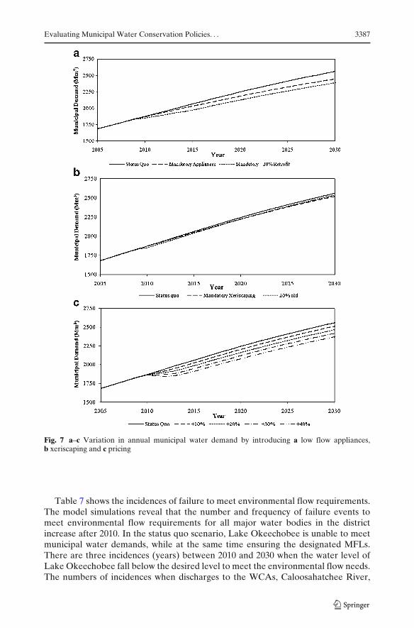
The status quo scenario assumes no changes in the current municipal water usepatterns during simulation time horizon. Precipitation and evapotranspiration ratesare also assumed to follow the historic average values. Figure 7a shows the variationof annual municipal demand from 2005 to 2030. It increases from 1,490 Mm3

(1.2 million ac-ft) in 2005 to 2,560 Mm3 (2.07 million ac-ft) in 2030 for an increaseof 72%.

Table 6 shows the performance evaluation results for Lake Okeechobee forvarious policies. For the status quo scenario, a reliability of 0.95 indicates that thelake levels stay above 3.35 m (11 ft) NGVD for 95% of the simulation time horizon.Thus, it fulfills all of its functions for 95% of the time. Resilience has a value of 1.31indicating that average duration of failure i.e., when the water level in the lake dropsbelow 3.35 m and recovers, is 1.31. Vulnerability, which represents the magnitude offailure, has a value of 0.41 for the status quo scenario. This implies that the lake levelson average drop below the 3.35 m (11 ft) mark by 0.41 feet per failure event.

Fig. 6 Comparison of historicdata and model simulations forLake Okeechobee water levels(m from NGVD) (calibration)

3.5

4.0

4.5

5.0

5.5

1975 1980 1985 1990 1995 2000 2005

Lak

e le

vels

(m

)

Years

Simulated Observed


Fig. 7 a–c Variation in annual municipal water demand by introducing a low flow appliances,b xeriscaping and c pricing

Table 7 shows the incidences of failure to meet environmental flow requirements.The model simulations reveal that the number and frequency of failure events tomeet environmental flow requirements for all major water bodies in the districtincrease after 2010. In the status quo scenario, Lake Okeechobee is unable to meetmunicipal water demands, while at the same time ensuring the designated MFLs.There are three incidences (years) between 2010 and 2030 when the water level ofLake Okeechobee fall below the desired level to meet the environmental flow needs.The numbers of incidences when discharges to the WCAs, Caloosahatchee River,


and St. Lucie Canal do not meet the designated environmental flows are four, four,and four, respectively.

5.4 Water Conservation policies to Reduce Municipal Water Demand

The municipal demand, as seen from the results of the status quo simulation,increases substantially from 2005 to 2030. Different policies are evaluated for theirpotential to decrease the municipal demand through conservation. These policiesinclude use of low flow appliances, reducing outdoor water consumption throughxeriscaping and price changes. All policies are implemented starting from 2010.

5.5 Low Flow Appliances

Conservation in indoor municipal water demand is evaluated by (1) mandatinginstallation of low flow appliances in all new homes constructed after 2010, and(2) retrofitting a selected percentage of existing homes with low flow appliances.The savings are applied independently for different types of domestic water uses(e.g., shower, toilets, faucet, laundry, and outdoor irrigation). Figure 7a shows thevariation of municipal water demand with the use of low flow appliances. Table 4shows the change in municipal demand due to the adoption of low flow appliancesin new homes, and separately, change in municipal demand when twenty percentof old homes are retrofit with low flow appliances. The water demand, due to theadoption of mandatory low flow appliances for new housing developments, dropsfrom 2,560 Mm3to 2,450 Mm3, for a savings of 4.3%. Retrofitting twenty percent ofthe old homes results in an annual water savings of 2.3%. Combined together, bothmeasures result in a savings of 170 Mm3 (141,000 ac-ft), a 6.64% reduction in annualmunicipal water demand by 2030.

5.6 Xeriscaping

The conservation in outdoor municipal water demand is evaluated by (1) mandatingxeriscaping in all new home constructed after 2010, and (2) converting a selectedpercentage of existing lawns to xeriscaping Fig. 7b shows the variation of municipalwater demand with xeriscaping.

Table 4 shows the change in municipal demand due to the adoption of xeriscapingin new homes, and when twenty percent of old homes are converted to xeriscaping.The water demand, due to the adoption of xeriscaping in new housing developments,drops from 2,560 Mm3 to 2,520 Mm3, for a savings of 1.6%. Converting twentypercent of existing lawns to xeriscaping results in 0.8% of annual water saving.Combined together, both measures result in a savings of 60 Mm3 (48,000 ac-ft), a2.34% reduction in annual municipal water demand by 2030.

5.7 Pricing

Figure 7c shows the variation of municipal water demand with price. Multiple modelsimulations are realized with water prices ranging from status quo to an increasein price of up to 40% at a 10% increment. As a result of price increase of 30% total


municipal water demand reduces from 2,560 Mm3to 2,420 Mm3, which translates into5.5% or 140 Mm3 (114,000 ac-ft) of municipal water savings per year by 2030.

5.8 Combined Policy

A combined policy scenario of low flow appliances, xeriscaping, and pricing areconsidered together. Figure 8 shows the reduction in municipal water demand dueto the combined policy. The water savings achieved by each policy are summarizedin Table 4. As a result, total municipal water demand reduces from 2,560 Mm3 to2,220 Mm3,which translates into 13.2% or 340 Mm3 (272,000 ac-ft) of municipal watersavings per year by 2030.

5.9 Achieving 5% Reduction in Municipal Water Demand

Table 5 shows the extent of implementation required for each policy option toachieve a 5% reduction in overall municipal water demand. Results show that a5% reduction in overall municipal water demand may be achieved through anyone of the following options: (1) retrofitting 58% of older homes with low flowappliances, (2) mandating low flow appliances in all new homes constructed after2010 and retrofitting 8.2% of old homes, (3) mandatory xeriscaping in all new homesconstructed after 2010 and changing existing lawns to xeriscaping in 88% of oldhomes, or (4) increasing price of water by 28%.

The maximum possible reduction in municipal water demand that can be achievedby each policy is also estimated and reported in Table 5. Results show that a pricehike of approximately 28% will result in an overall reduction of 5% in municipalwater demand. Retrofitting low flow appliances in all old homes offers the maxi-mum potential reduction, 11.7%, in municipal water demand. The second greatestreduction is through use of low flow appliances in all new homes constructed after2010 that results in 4.3% savings. Xeriscaping in old homes is ranked number three,

Fig. 8 Comparison of reduction in annual municipal water demand due to various water conserva-tion policies


and it offers 3.9% savings. Ranked last is mandatory xeriscaping in all new homeswith water savings of only 1.6%. Low flow appliance both in new and old homesprovide water savings almost three times (16%) greater than water savings offeredby xeriscaping both in new and old homes (5.5%). This is likely due to the fact that70% of water is used indoors in South Florida.

5.10 Population Growth

The future growth in population would translate into a growth in demand for freshwater. Considering the impacts of water withdrawals, it becomes imperative to assessthe impacts of growing population on water availability for fulfilling environmentalwater demands.

Population growth has a major impact on the total and municipal water demandsin the SFWMD. The increase in municipal water demand, as a result of populationgrowth, is 36.7% from 2010 to 2030 under the status quo scenario. However, if theregion experiences a growth greater than anticipated, then it will require additionalwater to meet municipal demands. Figure 9 shows the change in municipal waterdemand as a result of varying population growth rates. The annual municipal demandin 2030 for an accelerated growth rate increases to 2,720 Mm3 as compared to2,560 Mm3 for status quo growth rate. Thus a 10% increase in population growth rateover the period between 2010 and 2030 leads to an increase in the annual municipalwater demand by 6.3%. Similarly, in the case of a population growth rate that is 10%under the status quo growth rate, municipal demand in 2030 is 2,400 Mm3and thereduction in demand is 6.3%.

Fig. 9 Comparative graph for change in municipal water demand due to change in populationgrowth rate


5.11 Meeting Municipal Water Demands from Lake Okeechobee

Currently, only 4% of municipal water demand is fulfilled from surface watersources, the remaining 96% is withdrawn from ground water. Thus any change inpopulation growth rate or municipal water demand has negligible impacts on waterlevels in Lake Okeechobee.

Considering the possibility that ground water sources may not be able to meetthe increasing demand in the future, we ran scenarios where we divert a percentageof future demands (i.e., 10%, 20% and 30%) to surface water sources. This optionresults in increasing competition with agricultural demands and impacts the environ-mental water releases. We compared the system performance for these scenarios withand without implementation of conservation policies. Results of Lake Okeechobeeperformance and its ability to meet environmental flow requirements are reported inTables 6 and 7, respectively.

For example, in a scenario when 20% of future municipal demands are fulfilledfrom surface water sources, comparison of performance with status quo shows thatreliability decreases from 0.95 to 0.90, average duration of failure increases from1.31 months to 1.51 months, and average magnitude per failure increases from 0.41 ftto 0.47 ft. Comparison of performance with status quo, in terms of number of failuresto meet environmental flow requirements, shows that failure incidences duringsimulation time horizon (2005–2030) increase from 3 to 10 for Lake Okeechobeewater level, from 4 to 12 for flow to WCA’s, from 4 to 11 for Caloosahatchee River,and from 4 to 11 for St. Lucie Canal.

For the scenario of 20% future municipal demand from surface water scenario,when combined conservation policies are implemented, there is improvements inperformance indicators and a reduction in environmental flow violations. For ex-ample, reliability increases from 0.90 to 0.92, average duration of failure reducesfrom 1.51 months to 1.43 months, and average magnitude per failure reduces from0.47 ft to 0.44 ft. Comparison of performance in terms of number of failures to meetenvironmental flow requirements shows that failure incidences during simulationtime horizon (2005–2030) decrease from 10 to 8 for Lake Okeechobee water level,from 12 to 10 for flow to WCA’s, from 11 to 9 for Caloosahatchee River, and from11 to 9 for St. Lucie Canal.

5.12 Ongoing Water Conservation Efforts

There are multiple efforts going on in the region to conserve water that include,among others, water reuse and aquifer storage and recovery. Currently, 316 Mm3 ofmunicipal water is reused in South Florida, which is about 20% of the SFWMD’scurrent municipal water demand. The SFWMD anticipates that reuse will reach927 Mm3 by 2030 (about 36% of total municipal water demand in 2030). If this isachieved it will have a significant impact in terms of reducing demand for fresh water.

6 Summary and Conclusions

For a region that hosts a diversity of land use from natural wetlands to large urbanand agricultural areas, it is often a difficult task to balance all of the competing water


demands. Use of a simulation model allows for testing of different hypothesis and forevaluating the impacts of different policies for their potential to conserve water andmeet environmental flow requirements. A dynamic simulation model, using a systemdynamics modeling approach, is developed to estimate water availability and waterdemands in South Florida. Different water conservation policies to reduce municipalwater demand are evaluated using performance criteria of reliability, resilience, andvulnerability and for their ability to meet environmental flow requirements. Themodel is calibrated and simulations, on a monthly time step, are carried out upto 2030.

The model simulations show that the SFWMD, given its growth rate of waterconsumption, will suffer setbacks with regards to its objective of avoiding a conflictbetween the various competing uses. The water resources of the district will prove tobe insufficient to satisfy the growing demands of the region if the present growthrate is continued without significant effort to make the water use more efficient.Therefore, it is essential to use the existing sources of water more efficiently.

Considering that municipal water demand will rise with increases in populationand that the sources of water remain limited, any solution to water managementconflicts will require a focus on conserving water and reducing per capita waterdemand. Water conservation in municipal water sector can go a long way in resolvingthe conflict due to competing water demands.

Based upon the findings of this research, the following conclusions can be drawn(1) the status quo scenario leads to reduction in water supply to meet environmentalflow requirements and therefore is not acceptable, (2) water conservation measures,as evaluated, are effective in saving water and reducing the environmental flowfailures, (3) pricing appears to be a valuable instrument for reduction in waterdemand (4) use of low flow appliances offers the best potential to reduce waterdemand, and (4) xeriscaping offers a promising solution to reduce outdoor water use.Policy makers should consider a combined use of raising prices, mandating use of lowflow appliances and mandating xeriscaping to increase potential savings in municipalwater use. When raising the price of water a tiered structure should be used to avoidthe regressive nature of this policy.

We would also like to point out some limitations of this study. The focus was onwater quantity, water quality issues have not been addressed in the study. Althoughmultiple policies are tested for their potential to reduce municipal water demandand increase environmental flows, no economic analysis was performed to estimatethe cost of implementing the policies. A detailed economic analysis incorporating allcosts and who will pay them will help in prioritizing the policies for implementation.All models are simplifications of reality and require making assumptions, especiallywhen the future is simulated. There are inherent limitations in making those as-sumptions. There are numerous scenarios, especially socio-political changes that caninfluence the outcomes of this model. For example future growth, demand, andsupply trends may be different due to a recession in the economy, increases in marketprices for agricultural crops, adoption of desalination or increased water reuse, andchanges in the political situation such as US–Cuban relationships. Moreover, waterutilities and regional development boards when faced with water shortages oftenregulate the density of development, implement restrictions on water uses (such asoutdoor irrigation), or purchase or exchange water with other entities as needed. Wehave not incorporated these management options in the base model; however, the


model presented here allows the user to set-up and simulate these assumptions in awhat-if type scenario.

For this study SD proved to be a suitable tool to model a large system with areasonable degree of accuracy. In a single model, it was possible to use disparatedata and integrate science and decision making. The model provides the decisionmakers with an insight into the total system behavior rather than the behavior of theindividual components, thus facilitating more informed decisions.

Acknowledgements The funding for this work was provided by National Oceanic and At-mospheric Administration’s Social Application and Research Program (NOAA-SARP) AwardNA070AR4310324.

References

Abtew W, Obeysekera J, Irizarry-Ortiz M, Lyons D, Reardon A (2003) Evapotranspiration esti-mation for South Florida. In: Proceedings of ASCE world water & environmental resourcescongress, Philadelphia

Abtew W, Pathak C, Huebner RS, Ciuca V (2007) Chapter 2 hydrology of the South Floridaenvironment. In: Redfield G (ed) 2007 South Florida environmental report. South Florida WaterManagement District, West Palm Beach

Ahmad S, Simonovic S (2000) System dynamics modeling of reservoir operations for flood manage-ment. J Comput Civ Eng 14(3):190–198

Ahmad S, Simonovic S (2004) Spatial system dynamics: new approach for simulation of waterresources systems. J Comput Civ Eng 18(4):331–340

Ahmad S, Simonovic S (2006) An intelligent decision support system for management of floods.Water Resour Manag 20:391–410

Alaa A, Abtew W, Horn SV, Khanal N (2000) Temporal and spatial characterization of rainfall overcentral and south Florida. J Am Water Resour Assoc 36(4):833–848

Ali A, Abtew W (1999) Regional rainfall frequency analysis for central and Southern Florida. Tech-nical Publication WRE #380, Water Resources Evaluation Department, South Florida WaterManagement District, West Palm Beach

Chung G, Lansey K, Blowers P, Brooks P, Ela W, Stewart S, Wilson P (2008) A general water supplyplanning model: evaluation of decentralized treatment. Environ Model Softw 23(7):893–905

Davis LW (2008) Durable goods and residential demand for energy and water: evidence from a fieldtrial. RAND J Econ 39(2):530–546

Davis SM, Ogden JC (1994) Everglades: the ecosystem and its restoration. St. Lucie Press, DelrayBeach

Elshorbagy A, Jutla A, Barbour L, Kells J (2005) System dynamics approach to assess the sustain-ability of reclamation of disturbed watersheds. Can J Civ Eng 32:144–158

FAC (2006) Rule: 40E-8.221, minimum flows and levels: surface waters, Florida Administrative Code(FAC). http://www.flrules.org/gateway/RuleNo.asp?ID=40E-8.221

Florida Consensus Estimating Conference (2000) http://edr.state.fl.us/population.htmGao Y, Liu C (1997) Research on simulated optimal decision making for a regional water resources

system. Water Resour Dev 13(1):123–134Graham M, Turner GM, Baynes TM, McInnis BC (2009) A water accounting system for strategic

water management. Water Resour Manag 24(3):513–545Guo HC, Liu L, Huang GH, Fuller GA, Zou R, Yin YYA (2001) System dynamics approach for

regional environmental planning and management: a study for the Lake Erhai Basin. J EnvironManag 61:93–111

Hashimoto T, Stedinger JR, Loucks DP (1982) Reliability, resilience, and vulnerability criteria forwater resource system performance evaluation. Water Resour Res 18(1):14–20

Jesús R, Gastélum JR, Valdés JB, Stewart S (2009) A decision support system to improve waterresources management in the Conchos basin. Water Resour Manag 23(8):1519–1548

http://www.flrules.org/gateway/RuleNo.asp?ID=40E-8.221

http://edr.state.fl.us/population.htm


Kaminski LE (2004) Public sector water conservation: technology and practices outside theGreat Lakes—St. Lawrence Region. Great Lakes Commission. http://www.glc.org/wateruse/conservation/pdf/BestTechnologiesReport.pdf. Accessed 21 Nov 2008

Klein H, Hull JW (1978) Biscayne Aquifer, South East Florida. GS Water-Resources InvestigationReport, pp 78–107

Li L, Simonovic S (2002) System dynamics model for predicting floods from snowmelt in NorthAmerican prairie watersheds. Hydrol Process 16:2645–2666

Li L, Xu H, Chen X, Simonovic SP (2010) Streamflow forecast and reservoir operation performanceassessment under climate change. Water Resour Manag 24(1):83–104

Madani K, Mariño M (2009) System dynamics analysis for managing Iran’s Zayandeh-Rud RiverBasin. Water Resour Manag 23(11):2163–2187

Marella RL (2000) Water withdrawals, use, discharge, and trends in Florida. Scientific InvestigationsReport 2004-5151

Marella RL (2008) Water use in Florida, 2005 and trends 1950–2005 Fact sheet 2008-3080.http://pubs.usgs.gov/fs/2008/3080/

Mayer PW, DeOreo WB, Opitz EM, Kiefer JC, Davis WY, Dziegielewski B, Nelson JO (1999)Residential end uses of water. American Waterworks Association Research Foundation, Denver

Nelson J (1994) Water saved by single family Xeriscapes. In: 1994 AWWA annual conferenceproceedings, Novato, CA, pp 1763–1775

Nieswiadomy ML (1992) Estimating urban residential water demand: effects of price structure,conservation, and public education. Water Resour Res 28(3):609–615

Olmstead SM, Stavins RN, Hanemann WM (2007) Water demand under alternative price structure.J Environ Econ Manage 54:181–198

Parker GG, Fergson GE, Love SK (1955) Water resources of southeastern Florida with specialreference to the geology and ground water of the Miami area: US Geological Survey WaterSupply Paper 1255, p 965

Renwick ME, Green RD (2000) Do residential water demand side management policies measureup? An analysis of eight California water agencies. J Environ Econ Manage 40(1):37–55

Renwick M, Green R, McCorkle C (1998) Measuring the price responsiveness of residential waterdemand in California’s urban areas. Report prepared for the California Department of WaterResources, Sacramento

SAFE (Strategic Assessment of Florida’s Environment) (1995) Florida per capita water use.http://www.pepps.fsu.edu/safe/pdf/sc1.pdf. Accessed 23 Mar 2008

Saysel AK, Barlas Y (2001) A dynamic modeling of salinization on irrigated lands. Ecol Model139:177–199

SFWMD (2002) 2000–2001 Drought in South Florida. http://www.sfwmd.gov/org/ema/reports/drought_report_2001/index.htm

Simonovic SP (2002) World water dynamics: global modeling of water resources. J Environ Manag66:249–267

Simonovic SP, Ahmad S (2005) Computer based model for flood evacuation emergency planning.Nat Hazards 34:25–51

Simonovic SP, Fahmy H (1999) A new modeling approach for water resources policy analysis. WaterResour Res 35(1):295–304

Simonovic SP, Rajasekaram V (2004) Integrated analyses of Canada’s water resources: a systemdynamics model. Can Water Resour J 29(4):223–250

Smith SK (2005) Florida population growth: past present and future. Bureau of Economic andBusiness Research, University of Florida, Gainesville

Sovocool KA (2005) Xeriscape conversion study: final report. A report Submitted to SouthernNevada Water Authority, Las Vegas

Stave KA (2003) A system dynamics model to facilitate public understanding of water managementoptions in Las Vegas, Nevada. J Environ Manag 67:303–313

Sterman JD (2000) Business dynamics: systems thinking and modeling for a complex world.McGraw-Hill, New York

Testa A, Newton A (1993) An evaluation of landscape rebate program. In: AWWA conserv‘93proceedings, Mesa, pp 1763–1775

Tidwell VC, Passell HD, Conrad SH, Thomas RP (2004) System dynamics modeling for community-based water planning: application to the middle Rio Grande. Aquat Sci 66:357–372

Timmins C (2003) Demand-side technology standards under inefficient pricing regimes. EnvironResour Econ 26(1):107–124

USACE and SFWMD (1999) http://www.evergladesplan.org/facts_info/publications.aspx

http://www.glc.org/wateruse/conservation/pdf/BestTechnologiesReport.pdf

http://www.glc.org/wateruse/conservation/pdf/BestTechnologiesReport.pdf

http://pubs.usgs.gov/fs/2008/3080/

http://www.pepps.fsu.edu/safe/pdf/sc1.pdf

http://www.sfwmd.gov/org/ema/reports/drought_report_2001/index.htm

http://www.sfwmd.gov/org/ema/reports/drought_report_2001/index.htm

http://www.evergladesplan.org/facts_info/publications.aspx


Vedwan N, Ahmad S, Miralles-Wilhelm F, Broad K, Letson D, Podesta G (2008) Institutionalevolution in Lake Okeechobee Management in Florida: characteristics, impacts, and limitations.Water Resour Manag 22:699–718

Vickers A (2001) Handbook of water use and conservation: homes, landscapes, industries, busi-nesses, farms. WaterPlow Press, Amherst

Vickers A (2006) Perspectives—new directions in lawn and landscape water conservation. J AWWA98(2):56–61

Winz I, Brierley G, Trowsdale S (2009) The use of system dynamics simulation in water resourcesmanagement. Water Resour Manag 23(7):1301–1323

Xu ZX, Takeuchi K, Ishidaira H, Zhang XW (2002) Sustainability analysis for yellow river waterresources using the system dynamics approach. Water Resour Manag 16:239–261

Zwick PD, Carr MH (2006) Florida 2060: a population distribution scenario for the state ofFlorida. A research project prepared for the 1000 Friends of Florida. http://www.1000fof.org/PUBS/2060/Florida-2060-Report-Final.pdf

http://www.1000fof.org/PUBS/2060/Florida-2060-Report-Final.pdf

http://www.1000fof.org/PUBS/2060/Florida-2060-Report-Final.pdf

evaluating municipal water conservation policies using · pdf filewater resour manage (2010)...

Documents