evaluating particulate matter 2.5 in the yangtze river delta

BearWorks BearWorks

MSU Graduate Theses

Summer 2020

Evaluating Particulate Matter 2.5 in the Yangtze River Delta Evaluating Particulate Matter 2.5 in the Yangtze River Delta

Muhammad Abdullah Missouri State University, [email protected]

As with any intellectual project, the content and views expressed in this thesis may be

considered objectionable by some readers. However, this student-scholar’s work has been

judged to have academic value by the student’s thesis committee members trained in the

discipline. The content and views expressed in this thesis are those of the student-scholar and

are not endorsed by Missouri State University, its Graduate College, or its employees.

Follow this and additional works at: https://bearworks.missouristate.edu/theses

Part of the Earth Sciences Commons, Environmental Sciences Commons, and the Statistics

and Probability Commons

Recommended Citation Recommended Citation Abdullah, Muhammad, "Evaluating Particulate Matter 2.5 in the Yangtze River Delta" (2020). MSU Graduate Theses. 3560. https://bearworks.missouristate.edu/theses/3560

This article or document was made available through BearWorks, the institutional repository of Missouri State University. The work contained in it may be protected by copyright and require permission of the copyright holder for reuse or redistribution. For more information, please contact [email protected].

https://bearworks.missouristate.edu/

https://bearworks.missouristate.edu/theses

https://bearworks.missouristate.edu/theses?utm_source=bearworks.missouristate.edu%2Ftheses%2F3560&utm_medium=PDF&utm_campaign=PDFCoverPages

http://network.bepress.com/hgg/discipline/153?utm_source=bearworks.missouristate.edu%2Ftheses%2F3560&utm_medium=PDF&utm_campaign=PDFCoverPages




https://bearworks.missouristate.edu/theses/3560?utm_source=bearworks.missouristate.edu%2Ftheses%2F3560&utm_medium=PDF&utm_campaign=PDFCoverPages

mailto:[email protected]

EVALUATING PARTICULATE MATTER 2.5 IN THE YANGTZE RIVER DELTA

A Master’s Thesis

Presented to

The Graduate College of

Missouri State University

In Partial Fulfillment

Of the Requirements for the Degree

Master of Science, Geospatial Sciences

By

Muhammad Abdullah

August 2020

ii


Geology, Geography, and Planning

Missouri State University, August 2020

Master of Science

Muhammad Abdullah

ABSTRACT

Particulate Matter 2.5 (PM2.5) is a growing concern in industrialized countries. In China, high

concentrations of PM2.5 are causing devastating health and environmental effects for the people

living there. Coal-burning for domestic and industrial purposes is the main culprit for decreasing

air quality in China. The focus of this paper is on the Yangtze River Delta (YRD) located on the

eastern coast of China. Hourly PM2.5 readings from March 2015 to June 2016 were obtained

from 125 air quality monitoring stations (AQMS) in 23 cities in the YRD. In this study, PM2.5

readings were examined using TIBCO Spotfire and ArcGISPro. Space-time pattern analysis and

inverse distance weighting (IDW) were adopted in observing space-time trends and dispersion of

PM2.5 in the region. Inverse distance weighting (IDW) interpolation represents the distribution of

PM2.5 in YRD, with peak values greater than 61 ug/m3 observed across the study area in

December 2015, January 2016 and February 2016. Zhejiang had lower interpolated values in

comparison with Jiangsu and Shanghai. Based on the space-time pattern analysis, PM2.5

demonstrated a downtrend along the Yangtze River during the study period. Furthermore, a

relationship between global gridded weather type classification (GWTC-2) weather types was

examined with declining PM2.5 concentrations. The results show Humid (H), Humid Warm

(HW), and Warm (W) weather types are associated with declining levels of PM2.5 in Jiangsu and

Shanghai in March, April, May, June 2015. While in March, April, May, June 2016, Warm (W),

Humid (H), and Cold Front Passage (CFP) are associated with declining levels of PM2.5 in

Zhejiang and only Warm (W) in Jiangsu.

KEYWORDS: Particulate Matter 2.5, PM2.5, China, Yangtze River Delta, IDW, GWTC-2,

space-time pattern analysis, GIS

iii


By

Muhammad Abdullah

A Master’s Thesis

Submitted to the Graduate College

Of Missouri State University

In Partial Fulfillment of the Requirements

For the Degree of Geospatial Sciences

August 2020

Approved:

Xiaomin Qiu, Ph.D., Thesis Committee Chair

David R. Perkins, Ph.D., Committee Member

Judith L. Meyer, Ph.D., Committee Member

Julie Masterson, Ph.D., Dean of the Graduate College

In the interest of academic freedom and the principle of free speech, approval of this thesis

indicates the format is acceptable and meets the academic criteria for the discipline as

determined by the faculty that constitute the thesis committee. The content and views expressed

in this thesis are those of the student-scholar and are not endorsed by Missouri State University,

its Graduate College, or its employees.

iv

ACKNOWLEDGEMENTS

I wish to express my deepest gratitude to everyone who gave me support throughout this

research project. Firstly, I would like to thank my committee chair, Dr. Qiu, who not only helped

me excel in my application of innovative GIS methods through this research but also provided

me with the opportunity to teach our future leaders the everyday importance of GIS.

I would like to thank Dr. Perkins and Dr. Meyer, who collectively, enhanced my

application of sustainability in my research and everyday life. Furthermore, I would like to

especially thank Dr. Mario Daoust for motivating me to pursue a Master’s of Science at our

prestigious institution. I would also like to thank my fellow peers from our department,

especially Jordan Vega and Charlie Hoffman, who supported me over the last two years.

Finally, I would like to thank my parents for the unconditional love and support they gave

me over the last six years of my life. Accomplishing this feat would be impossible if it was not

for Dr. Abdur Rehman Jami and Shazia Abdur Rehman. Thank you for everything.

v

TABLE OF CONTENTS

Introduction

1

Literature Review 3

Particulate Matter 3

Harmful Effects of PM2.5 5

Regulatory Policies in China 7

Meteorological Conditions and PM2.5

9

Materials and Methodology 12

Study Area 12

Data Source 13

Methods

14

Results 20

TIBCO Spotfire 20

Inverse Distance Weighted Interpolation 22

Space-Time Pattern Mining 23

Multiple Linear Regression Analysis

24

Discussion

35

Conclusions

39

References

40

Appendices 46

Appendix A: Power Stations – Jiangsu, Shanghai, Zhejiang 46

Appendix B: GWTC-2 - Jiangsu, Shanghai, Zhejiang 48

vi

LIST OF TABLES

Table 1: The 11 GWT-2 Weather Types

10

Table 2: Air Quality Index (AQI)

17

Table 3: Multiple Linear Regression Summary Table (2015)

26

Table 4: Multiple Linear Regression Summary Table (2016)

26

vii

LIST OF FIGURES

Figure 1: China vs. global coal consumption

2

Figure 2: Satellite image of smog covering eastern China

10

Figure 3: Averaged PM2.5 concentrations of 190 cities

11

Figure 4: Location of Yangtze River

17

Figure 5: Operating coal power stations locations with heatmap

18

Figure 6: AQMS locations in YRD

18

Figure 7: Cities with AQMS in YRD

18

Figure 8: Illustration of space-time cube

19

Figure 9: Illustration of space-time bin

19

Figure 10: Monthly mean PM2.5 (a) Jiangsu (b) Shanghai (c) Zhejiang

27

Figure 11: Monthly PM2.5 readings (a) Jiangsu (b) Shanghai (c)

Zhejiang

28

Figure 12: Tibco Spotfire: AQI levels – Jiangsu

29

Figure 13: Tibco Spotfire: AQI levels – Shanghai

29

Figure 14: Tibco Spotfire: AQI levels – Zhejiang

30

Figure 15: IDW: March – June (2015)

30

Figure 16: IDW: July – October (2015)

31

Figure 17: IDW: November and December (2015); January and

February (2016)

31

Figure 18: IDW: March – June (2016)

31

Figure 19: Visualizing time-cube in 2D

32

Figure 20: Emerging hot spot analysis

33

Figure 21: GWTC-2 avg. PM2.5 (spring-to-summer 2015 and 2016):

Shanghai

34


Zhejiang

34


Jiangsu

34

1

INTRODUCTION

Since the Industrial Revolution, countries such as China, the United States of America

(USA), and Russia (formerly known as USSR) have gained great economic wealth as a result of

their highly industrialized economies. In 2018, IMF reported that China's economy generated

$25.3 trillion, making it the world’s largest economy (CRS, 2019). China's reliance on its coal

reserves is a key factor driving its economic success. According to a report published in 2013 by

Mining-Technology, China's coal reserves in 2012 stood at 115 billion tons (Bt) trailing the USA

and Russia at 237 Bt and 157 Bt, respectively. Furthermore, China is the biggest coal importer in

the world as it imported 289 million tons (Mt) of coal that year (Mining-Technology, 2014).

China consumes more coal than all the world's countries combined, resulting in reduced air

quality (China Power Project, 2016). Figure 1 displays China’s growing coal consumption from

1965 to 2015.

Acute levels of air pollution have become a cause for significant concern in industrialized

and urban settings of developing nations (Nagpure, Gurjar, & Martel, 2014; Shu et al., 2017;

Xing, Xu, Shi, & Lian, 2016). The Ambient Air Quality Standards that are currently effective in

China, were released by the Ministry of Environmental Protection on February 29, 2012 (LOC,

2018). The standards set mandatory limits for the primary pollutants – sulfur dioxide (SO2),

nitrogen dioxide (NO2), carbon monoxide (CO), ozone (O3), particulate matter 10 (PM10), and

particulate matter 2.5 (PM2.5) – and took effect nationwide on January 1, 2016. The standards set

two classes of limit values:

• Class I: the limit set at 35 µg/m3 daily mean per city, apply to regions needing

special protection such as nature reserves and natural scenic areas.

• Class II: limit set 75 µg/m3 daily mean per city, apply to all other areas including

residential, mixed-use, industrial, and rural areas.

2

Identifying how airborne particulate matter as it relates to the health of the population is

complex. Earlier studies (Pope III et al., 2002; Rahman, & MacNee, 1996; Schwartz, 2000)

determined that PM levels contribute to significant human health concerns and environmental

degradation, while more recent studies have looked at developing unique techniques in dealing

with this issue (Brook et al., 2010; Cesaroni et al., 2014; Hussey et al., 2017; Krewski et al.,

2009; Lim et al., 2012; Mohapatra & Biswal, 2014; Nawrot, Perez, Künzli, Munters, & Nemery

2011; Xing et al., 2016).

The present research evaluates PM2.5 concentrations using hourly PM2.5 readings

monitored by 125 air quality monitoring stations (AQMS) in the Yangtze River Delta (YRD).

Data were collected from March 2015 to June 2016 in 23 cities within the YRD. The readings

were spatially analyzed using inverse distance weighted (IDW) interpolation and space-time

pattern mining tools in ArcGIS Pro. The relationship of the global gridded weather typing

classification (GWTC-2) (Lee, 2015b) and its effect on PM2.5 was then explored. All of these

provide an understanding of how widespread the issue of PM2.5 was in the YRD, which can be

used to help the local governments reduce air pollution.

Figure 1: China vs. global coal consumption (China Power Project, 2016)

3

LITERATURE REVIEW

Particulate Matter (PM)

Particulate matter (PM) is a widespread pollutant made of all solid and liquid particles

suspended in air -- many of which are hazardous to human health (Arita & Costa, 2011). This

complex mixture includes both organic and inorganic particles, such as dust, pollen, soot, smoke,

and liquid droplets. Common chemical components of PM include sulfates, nitrates, ammonium,

and other inorganic ions such as ions of sodium, potassium, calcium, magnesium, and chloride,

organic, and elemental carbon, crustal material, particle-bound water, metals (including

cadmium, copper, nickel, vanadium, and zinc), and polycyclic aromatic hydrocarbons (PAH)

(WHO, 2013). Furthermore, biological components such as allergens and microbial compounds

are found in PM (Kalisa et al., 2019). PM varies significantly in size, composition, and origin.

Commonly used indicators describing PM that are relevant to health, refer to the mass

concentration of particles with a diameter fewer than 10 micrometers as coarse particulate matter

or PM10 and particles with a diameter of fewer than 2.5 micrometers as fine particulate matter or

PM2.5.

The particles in the air are either directly emitted or indirectly formed. Primary PM and

gaseous predecessors such as oxides of nitrogen, ammonia, and non-methane volatile organic

compounds (secondary particles) have both anthropogenic and natural sources. Anthropogenic

sources include combustion for energy production in households and industrial activities. This

combustion for energy includes construction, ceramic production, smelting, manufacture of

cement, agriculture, and mining, which is particularly a concern in China. Secondary particles

found in PM2.5 are formed through chemical reactions of gaseous pollutants, e.g. the chemical

4

transformation of nitrogen oxides (from traffic and industrial processes) and the combustion of

sulfur-containing fuels. Furthermore, long-range transport of dust is also an element of

particulate matter (William, M.H., & William R.B., 2004) . Figure 2 shows acute levels of smog

covering eastern China during the winter months in 2013. Fine particles or particulate matter 2.5

(PM2.5) tend to stay in the atmosphere longer than the coarse particles, or particulate matter 10

(PM10). This increases the chance of humans and animals inhaling them into their bodies and

thus causing devastating health effects (WHO, 2003). To remedy concerns about PM emissions,

electrostatic precipitators are used in many Chinese coal-fired power plants; however, they are

generally only effective for PM10, as most of them do not have a high collective efficiency of

PM2.5 (Pui, Chen, & Zuo, 2014).

According to the World Health Organization (WHO), less than 1% of the 500 largest

cities in China met the air quality guideline in 2013 (10 ug/m3 for annual mean and 25 ug/m3 for

a 24-hour mean). Seven of these cities are ranked among the ten most polluted cities in the world

(Zhang & Cao, 2015). Figure 3 shows the study conducted by Zhang and Cao in 2015, where

they averaged seasonal fine particulate matter concentrations of 190 cities in China. The annual

average concentration of PM2.5 was 57+- 18 ug/m3, exceeding the new National Ambient Air

Quality Standard (NAAQS) (35 ug/m3) of China and WHO air quality guidelines (10 ug/m3).

The findings show that the winter season had the highest average concentration of PM2.5 which

was associated with intensified anthropogenic emissions from fossil fuel combustion and

biomass burning. In addition, unfavorable meteorological conditions, such as temperature

inversions, also played a role in pollution dispersion (Zhang & Cao, 2015). A study conducted in

2018 by Id et al. provides further insight into the sources of PM2.5 emissions in the Yangtze River

Delta (YRD). The authors concluded that PM2.5 sources were both local and regional in nature as

5

64% of emissions were from local sources, and 36% of emissions were from circumjacent

regions. Furthermore, corresponding to modeling scenarios where all anthropogenic emissions

were proportionally reduced, the authors’ results demonstrated a nearly linear correlation

between anthropogenic emissions reduction and the PM2.5 concentration decrease: a 10%

reduction in anthropogenic emissions resulted in a 10% reduction in PM2.5 concentration. A 20%,

30%, 40%, or 50% reduction in anthropogenic activities showed a corresponding PM2.5

concentration reduction by 19%, 28%, 37%, or 46% respectively.

Harmful Effects of PM2.5

Health Issues. Short-term and long-term exposure to PM2.5 is harmful to the human

body. Several studies have linked particle pollution exposure to a variety of health problems.

This includes premature death in people with heart or lung diseases, non-fatal heart attacks,

aggravated asthma, decreased lung function, and increased respiratory symptoms (EPA, 2016). It

is estimated that approximately 3% of cardiopulmonary and 5% of lung cancer deaths are

attributable to PM globally (WHO, 2009). Daily mortality is estimated to increase by 0.2–0.6%

per 10 μg/m3 of PM10 (Samoli et al., 2008). Long-term exposure to PM2.5, a higher risk factor in

comparison to PM10, is associated with an increase in the long-term risk of cardiopulmonary

mortality by 6–13% per 10 μg/m3 of PM2.5 (Krewski et al., 2009). This is particularly worse for

individuals with pre-existing lung and heart conditions, children, and elderly populations (Brook

et al., 2010). PM2.5 can penetrate deep into the lungs, irritating, and corroding the alveolar wall

leading to decreasing lung function (Xing et al., 2016). According to the Global Burden of

Disease (GBD) assessment, long-term exposure to PM2.5 contributes to 3.2 million deaths

globally each year, ranking it as the sixth-largest contributor to the GBD (Lim et al., 2012). Fine

6

particulate matter (PM2.5) causes vascular inflammation and atherosclerosis as PM2.5 leads to high

depositions of plaque in arteries, solidifying the arteries and reducing elasticity, leading to heart

attacks and other cardiovascular problems (Pope III et al., 2002). In the results of the European

Study of Cohorts for Air Pollution Effects (ESCAPE), 11 groups totaling 100,166 participants

were followed for an average of 11.5 years and showed a 13% increased risk of heart attacks

linked to an increase in estimated exposure of PM2.5 by 5 μg/m3 (Cesaroni et al., 2014). PM not

only affects human cells and tissues but also impacts bacteria that cause disease in humans

(Hussey et al., 2017). Hussey et al.'s study (2017) concluded that biofilm formation, antibiotic

tolerance, and colonization of both Staphylococcus aureus and Streptococcus pneumonia

bacteria was altered by PM exposure.

Exposure to fine particulate matter (PM2.5) during pregnancy is associated with high

blood pressure in children (Zhang et al., 2018) as well as other physiological problems such as

inflammation, oxidative stress, endocrine disruption, and impaired oxygen transport access to the

placenta (Erickson & Arbour, 2014). All of these are mechanisms that can increase the risk of

low birth weight (Lee et al., 2012). Toxicological and epidemiologic evidence suggests that a

strong relationship exists between long-term PM2.5 exposure and cardiovascular effects (EPA,

2009a). According to Li et al. (2017), an estimated 4,172 non-accidental deaths in Beijing alone

in 2015 are attributed to long-term PM2.5 exposure. China lacks strict ambient air control policies

and these statistics are alarming, considering the population of the country.

Climatic Effects. Particulate matter (PM) contributes to cloud formation, playing a role

in the greenhouse effect and climate change (Mohapatra & Biswal, 2014). The amount of solar

radiation and outgoing terrestrial longwave radiation is affected by atmospheric aerosols (Ayash,

Gong, & Jia, 2009). Atmospheric aerosols control Earth’s climate by influencing the radiation

7

budget at regional and global scales (Krishna et al., 2018). They directly influence the climate by

absorbing and scattering the incoming solar radiation (Charlson et al., 1992). Atmospheric

aerosols also influence climate indirectly by altering the cloud microphysics (Twomey, 1974).

The aerosol-climate effects are considered the largest source of uncertainty in future climate

predictions (Boucher et al., 2013).

Environmental Effects. Depending on the chemical constituents of the particulate

matter, PM can result in the acidification of lakes and streams, alter the nutrient balance in

coastal waters and large river basins, deplete the nutrients in the soil, damage sensitive forests

and farm crops, and negatively affect the diversity of ecosystems (EPA, 2019). Acid rain has a

damaging effect on infrastructure by accelerating the weathering of buildings and outdoor

sculptures and statues (Nguyen, 2018). Furthermore, PM2.5 is responsible for the smog that can

be seen in both urban and rural regions (Jin, Luo, Fu, & Li, 2017). Smog is characterized by high

PM2.5 levels and reduced visibility and has been reported in China, especially in developed and

high city clusters such as the YRD (Zhang & Cao, 2015).

Regulatory Policies in China

Since the initial passage of the framework Environmental Protection Law in 1979, China

has enacted many laws, regulations, and standards addressing environmental protection.

Executing the environmental protection laws efficiently has been difficult, however, it has

become increasingly robust over the past few decades since severe air pollution has caused

colossal health and social costs. The social costs of air pollution extend far beyond health,

including climate, water, renewable energy, and agriculture (Seddon, Contrerars, & Elliot, 2019).

The primary law dealing with air pollution, Air Pollution Prevention and Control Law, provides

8

comprehensive measures on air pollution prevention and control (LOC, 2018). The government

has recognized that air pollution is severe and that the pressure to control pollution is expected to

increase due to growing energy consumption resulting from industrialization and urbanization of

the country (CAAC, 2013). Air pollution has been addressed in a series of national policies,

including the national five-year plan (2016 - 2020) for economic and social development which

set clean air-targets for the country with corresponding time limits (LOC, 2018). The State

Council of China issued the Air Pollution Prevention and Control Action Plan in September

2013. The Action Plan guides national efforts to control air pollution in the present and near

future by setting quantitative targets for improving the air quality of the whole country and of

key regions within specified time limits -- this includes heavily polluted regions such as the

Yangtze River Delta, where PM2.5 concentrations must fall by 20% by 2017 (LOC, 2018).

According to the Environmental Protection Law and the Air Law, the environmental

protection agency under the State Council is tasked with formulating national environmental

quality standards, including air quality standards. Provincial governments may establish local

standards on items not covered in the national standards and set stricter limits on items covered

by national standards. Regions that have not met the national standards must formulate an

attainment plan showing how they will meet the standards by a specific time. Although this

demonstrates that China is heading in a direction tackling the issue of air pollution, PM2.5

concentrations are still a concern. According to a report submitted by China's top legislature, Li

Ganjie, the country's Ecology, and Environment Minister, 256 out of 365 cities nationwide

exceeded the national secondary standard (35 ug/m3), accounting for 70% of the total number of

cities (Greenpeace China, 2018).

9

Meteorological Conditions and PM2.5

Meteorological conditions greatly influence PM2.5 pollution. Regions with high PM2.5

levels in China had unfavorable meteorological conditions, such as low wind speed, high

humidity, and low rainfall (Xu et al., 2018). Furthermore, Xu et al. (2018) established a

relationship between PM2.5 and meteorological factors from January 2016 to January 2017

among key regions of China of Beijing-Tanjian-Heibei (JJJ), Pearl Delta (PRD), Chengdu-

Chongqing (CYB), and Yangtze River Delta (YRD) regions. The study concluded that the

meteorological conditions in JJJ, PRD, and CYB regions contributed to PM2.5 worsening by

29.7%, 42.6%, and 7.9% respectively. However, in YRD the meteorological conditions

contributed to better air quality, improving by approximately 8.5% from January 2016 to January

2017. Increased wind frequency and more ocean currents contributed to low PM2.5 concentrations

in YRD.

The global gridded weather typing classification (GWTC-2) system is a geographic and

seasonal-relative classification of multivariate surface weather conditions, i.e., weather types.

The GWTC-2 system is based upon the gridded weather typing classification (GWTC) system

built for North America. It uses six weather variables: temperature, dew point, sea-level pressure,

cloudiness, wind speed, and wind direction (Mesinger, Dimego, Oceanic, & Mitchell, 2006).

Table 1 represents the 11 weather types, with 9 being “core weather types” relating to different

temperature and humidity conditions. The two transitional weather types identify the passage of

traditional cold fronts and warm fronts (Lee, 2015b). The idea behind the GWTC-2 classification

system is based on a “feels-like” classification. For example, say in Dubai, U.A.E in mid-June

the daytime high temperature is 61°F (16°C). People in Dubai would consider that to be quite

cold for the time of the year. However, someone living in the state of Michigan, U.S.A, would

10

describe the same temperature as warm. Similarly, if the same scenario were to happen in mid-

December in Dubai, the locals would think it is quite warm for winter. What makes GWTC-2

different from other classifications is that it classifies multivariate surface weather situations

relative to a climatological normal. Associating GWTC-2 weather types to human health and

other biological systems might respond to multivariate departures from normal more-so than raw

meteorological conditions (Lee, 2015a).

Increasing Humidity Increasing Temperature

Humid Cool (HC) Humid (H) Humid Warm (HW)

Cool (C) Seasonal (S) Warm (W)

Dry Cool (DC) Dry (D) Dry Warm (DW)

Cold Frontal Passage

(CFP)

Warm Front Passage

(WFP)

Table 1. The 11 GWTC-2 weather types (Lee, 2015b).

Figure 2: Satellite Image of smog covering Eastern China on December 7, 2013. NASA obtained

this image using Terra satellite with a Moderate Resolution Imaging Spectroradiometer

(MODIS) sensor.

11

Figure 3: a) The averaged PM2.5 concentrations (ug/m3) of the 190 cities of China, during the

year of 2014/2015 and b) during spring, c) summer, d) autumn and e) winter (Y. L. Zhang et al.,

2015).

12

MATERIALS AND METHODOLOGY

Study Area

The Yangtze River Delta (YRD) area is composed of Jiangsu province, Zhejiang

province, and the city of Shanghai. The terrain in YRD is generally flat and low-lying floodplain

with hilly areas in Hangzhou located in Zhejiang province. The YRD region has a marine

monsoon subtropical climate with hot and humid summers, cool and dry winters (Gu, Hu, Zhang,

Wang, & Guo, 2011). Rapid urbanization in the YRD has transformed this area into a key

economic region, covering a total area of 81,350 mi2 (Jiangsu: 39,600mi2, Zhejiang: 39,900 mi2,

Shanghai: 2,450 mi2), 1% of the total land area of China, and home to over 162 million people

(China National Bureau of Statistics, 2018). The Yangtze River flows through Jiangsu and into

the East China Sea through the Yangtze River Delta as seen in Figure 4. Figure 5 shows the

operating coal power stations in Jiangsu and Zhejiang provinces, with 76 and 23 respectively.

Shanghai, a logistics and financial center in mainland China, has only eight operation coal power

stations (Global Energy Monitor, 2020). The heatmap in Figure 6, shows the highest energy

generated in the coal power stations is located along the Yangtze River, indicating high levels of

economic activity. Appendix A-1, A-2, and A-3 show the total number of operating units and

power stations in the YRD. Jiangsu province had a GDP of $1.2 trillion followed by Zhejiang

province at $735.3 billion and Shanghai at $425.6 billion in 2017 (Textor, 2020). Major

industries contributing to the GDP of YRD include electronics, chemicals, textiles, steel, metal

fabrication, automobiles, petrochemicals, and power generation (International Trade

Administration, 2014). Nearly 22% of China's GDP, with an average annual economic growth of

20%, is concentrated in the YRD (Shanghai Expo, 2020).

13

Data Source

This study focuses on PM2.5, one of the six pollutants (SO2, NO2, CO, O3, PM10, and

PM2.5) recorded by the AQMS in the YRD. The hourly pollutant readings were obtained from

March 2015 – June 2016 through the assistance of Dr. Xiaomin Qiu. The readings were

measured in micrograms (ug/m3). Figure 6 shows the locations of 125 AQMS in 23 cities within

the YRD where data was collected for this study. Jiangsu and Zhejiang provinces had 73 and 44

AQMS while Shanghai only had 8 AQMS. The 23 cities in this study are shown in Figure 7. An

Air Quality Index (AQI), issued by EPA (2009b), comprises of six levels evaluating all six air

pollutants (Table 2): good (Grade I, 0–50 ug/m3), moderate (Grade II, 51–100 ug/m3), unhealthy

for sensitive groups (Grade III, 101–150 ug/m3), unhealthy (Grade IV, 151-200 ug/m3), very

unhealthy (Grade V, 201–300 ug/m3) and hazardous (Grade VI, 301-500 ug/m3). The value 100

ug/m3 is considered the acceptable standard from a public health perspective where few

hypersensitive individuals should reduce outdoor exercise. Hence, the Grade II standard has been

widely used and generally accepted by governments and the public. It is a critical ambient air

quality standard for judging whether air pollution is out of limits.

At each monitoring site, the real-time concentrations of PM2.5 are measured using the beta

ray absorption method (BAM) from commercial instruments and/or the tapered element

oscillating microbalance (TEOM) ( Jakowiuk, Urbański, Świstowski, Machaj, & Pieńkos, 2008);

Patashnick & Rupprecht, 1991). The beta ray absorption (BAM) technique employs the

absorption of beta radiation by solid particles extracted from the airflow, which allows for the

detection of PM2.5 (Jakowiuk et al., 2008). In contrast, TEOM collects PM on a vibrating

substrate and measures the change in the oscillation frequency that decreases with mass loading

(Patashnick & Rupprecht, 1991). Another requirement in the data collection by the AQMS is that

14

they must be a thousand meters clear of tall buildings, trees, or other obstructions that could

impede air circulation. The AQMS data was observed at 3-15 meters above ground in open areas

with no emission sources (She et al., 2017).

Methods

Data Visualization. TIBCO Spotfire is a data visualization tool that allows us to access

and combine data in a single analysis and get a holistic view of interactive visualization. TIBCO

Spotfire allowed the processing of large amounts of hourly PM2.5 information stored in MS Excel

at once. It generated maps, observing spatial trends of PM2.5 in each AQMS provincially. Figures

with monthly mean and all readings of PM2.5 provincially were also produced.

Inverse Distance Weighted (IDW) Interpolation. Prior studies have utilized numerous

interpolation techniques that are used to create a continuous surface from sampled point values in

estimating PM. Interpolation methods such as spatial averaging, nearest neighbor, inverse

distance weighting (IDW), and Kriging have been used (Krewski et al., 2009; Wong, Yuan, &

Perlin, 2004). These interpolation tools are divided into two methods: (1) geostatistical and (2)

deterministic interpolation. Geostatistical techniques create a prediction surface and provide

some measures of the certainty or accuracy or predictions, e.g. Kriging interpolation.

Deterministic interpolation methods assign values to locations based on the surrounding

measured values and on specified mathematical formulas that determine the smoothness of the

resulting surface (ESRI, 2016). These methods include inverse distance weighting (IDW), the

interpolation technique used in this study.

Based on Tobler’s First Law of Geography, where things close to one another share more

similarities than those afar (Tobler, 1970), the IDW technique calculates an average value for

15

unsampled locations using values from nearby weighted locations. The weights are proportional

to the proximity of the sampled points to the unsampled location and can be specified by the

IDW power coefficient. The larger the power coefficient, the stronger the weight of nearby

points as can be gathered from the following equation that estimates the value z at an unsampled

location j:

The carat (^) above the variable z reminds us that we are approximating the value at j. The

parameter n is the weight parameter that is applied as an exponent to the distance thus

magnifying the irrelevance of a point at location i as the distance to j increases. Nearby points

wield greater influence on unsampled locations than a point further away when the n value is

large. In contrast, a small n value generates all points within the search radius equal weight such

that all unsampled locations will represent nothing more than the mean values of all sampled

points within the search radius (Gimond, 2019). In summary IDW interpolation involves: (a)

defining the search area or neighborhood around the point to be predicted; (b) locating the

observed data points within this neighborhood; and (c) assigning appropriate weights to each of

the observed data points (Wong et al., 2004).

Space-Time Pattern Mining. Further analysis involves the application of the space-time

pattern mining toolbox in ArcGIS Pro. Space-time analysis considers both location and time

when determining patterns and relationships to provide a better understanding of a geographic

phenomenon (ESRI, 2019b). This toolbox answers data where geography does not change, but

the PM2.5 readings associated with it change over time. Space-time pattern mining facilitates an

examination of intricate data trends that prevail across an area and vary over time. For example,

16

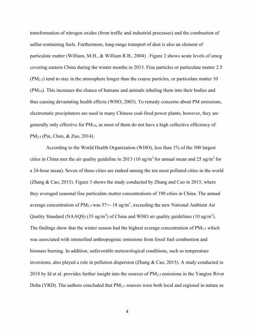
a space-time cube created from defined locations can structure data into a NetCDF (a

multidimensional dataset where defined locations are aggregated) data format by creating space-

time bins as seen in Figure 8 (ESRI, 2020). Every bin has a fixed position in space (x and y

values) and in time (t) (Figure 9). The hourly PM2.5 data for each station was aggregated into a

monthly time-step interval to understand the PM2.5 variation over the study period. Once the

space-time cube is created, it was visualized in 2D helping understand monthly trends at each

station. Furthermore, the emerging hot spot analysis tool in the space-time toolbox recognized

the pattern of these trends. This tool identified hot spot (rising PM2.5 levels) and cold spot (falling

PM2.5 levels) patterns. These hot and cold spot patterns were categorized in the following manner

(ESRI, 2019a):

• Sporadic Hot Spot Pattern: present at AQMS with an on-again then off-again

hotspot. Less than 90% of the time-step intervals are statistically significant hot

spots and none of the time-step intervals are statistically significant cold spots.

• Oscillating Hot Spot Pattern: statistically significant hot spot for the final time-

step interval and had a history of being a statistically significant cold spot during a

prior time-step. Less than 90% of the time-step intervals have been statistically

significant hot spots.

• Persistent Cold Spot Pattern: present at AQMS that have been statistically

significant cold spots for 90% of the time-step intervals with no observable trend

indicating an increase or decrease in the intensity of values over time.

• Sporadic Cold Spot Pattern: present at AQMS that is an on-again then off-again

cold spot. Less than 90% of the time-step intervals are statistically significant cold

spots and none of the time-step intervals are statistically significant hot spots.

• Oscillating Cold Spot Pattern: statistically significant cold spot for the final time-

step interval and had a history of being a statistically significant hot spot during a

prior time-step. Less than 90% of the time-step intervals have been statistically

significant cold spots.

• No Pattern Detected: Does not fall into any of the hot or cold spot patterns.

Multiple Linear Regression Analysis. Daily average PM2.5 readings in the months of

March, April, May, and June 2015 and 2016 with the 11 GWTC-2 weather types classified as

dummy variables were analyzed by multiple linear regression. The dummy variables took the

17

value 0 or 1 to indicate the presence or absence of the GWTC-2 variables' categorical effect that

may shift the outcome. The months of March, April, May, and June were selected for both years

as they allowed for a comparison of the PM2.5 and the GWTC-2 variables over the sixteen-month

study period. The starting and ending months acted as “transitionary months” with March going

to spring from the winter season and June fading into summer from the spring season. The

multiple linear regression analysis helped understand the GWTC-2 weather types affecting

PM2.5.

Air Quality Index (AQI) by EPA

Values of Index (ug/m3) Levels of Concern Daily AQI Color

0 – 50 Good Green

51 – 100 Moderate Yellow

101 – 150 Unhealthy for Sensitive Groups Orange

151 – 200 Unhealthy Red

201 – 300 Very Unhealthy Purple

301 – 500 Hazardous Maroon

Table 2. Air Quality Index (AQI) by the EPA containing the six levels of evaluating air quality.

Figure 4: Location of the Yangtze River.

18

Figure 5: Operating coal power station in YRD with annual energy generated in Megawatts

(MW) (Global Energy Monitor, 2020).

Figure 6: AQMS locations in YRD. Jiangsu

Province (76 AQMS); Zhejiang province (44

AQMS); Shanghai (8 AQMS).

Figure 7: Cities with AQMS observed in the

study.

19

Figure 8: Illustration of Space-time cube (ESRI, 2020).

Figure 9: Illustration of Space-time bin. Every bin has a position in space (x and y) and time (t).

(ESRI, 2019a).

20

RESULTS

TIBCO Spotfire

The PM2.5 levels showed significant monthly variation with the warmer months

displaying low levels of pollutants in contrast to the cooler months, where the entire region

displayed high levels of pollutants. Enhanced emissions from fossil fuel combustion, biomass

burning for domestic heating, and “unfavorable” metrological conditions contribute to the

pollution dispersion. An example of unfavorable meteorological conditions is when cold weather

makes it difficult for car emission control systems to operate effectively (She et al., 2017).

Temperature inversion plays a key role, as a dense layer of cold air gets trapped under a layer of

warm air which acts as a lid, trapping PM2.5 in the cold air near the ground and as a result

limiting diffusion of air pollutants (TCHD, 2016).

As observed in Figure 10 (a), (b), and (c), the highest monthly averages were observed in

December 2015 for Jiangsu, Shanghai, and Zhejiang at 93 ug/m3, 106 ug/m3, and 75 ug/m3

respectively. Zhejiang compared with Jiangsu and Shanghai, has a relatively lower monthly

mean for December 2015. In contrast, the lowest mean PM2.5 readings in Jiangsu, Shanghai, and

Zhejiang were at 34 ug/m3 (September 2015), 51ug/m3 (May 2015), and 29 ug/m3 (July 2015)

respectively.

Figures 11 (a), (b), (c) display the readings in ug/m3 on the y-axis and months on the x-

axis. Jiangsu province recorded the highest reading at 789 ug/m3 in February 2016, which is

greater than EPA’s hazardous level (Grade VI, 301-500 ug/m3). In contrast to Jiangsu, Shanghai

recorded a high of 237 ug/m3 in December 2015 while Zhejiang province had the highest

recorded in January 2016 at 438 ug/m3. It is important to note that all these values were recorded

21

in the winter months of December 2015, January 2016, and February 2016. Figure 12 displays

the AQI levels in the Jiangsu province. The criteria were set at good (Grade I, 0–50 ug/m3),

moderate (Grade II, 51–100 ug/m3), unhealthy for sensitive groups (Grade III, 101–150 ug/m3),

unhealthy (Grade IV, 151–200 ug/m3), very unhealthy (Grade V, 201–300 ug/m3) and hazardous

(Grade VI, 301-500 ug/m3). We can see that Grades I-VI were observed at every station over the

course of the study. However, readings greater than Grade VI were observed in AQMS in

Taizhou, Nantong, Wuxi, Suzhou, Xuzhou, and Lianyungang. Shanghai, recorded readings

between Grade I-V (Figure 12). We can see in Figure 13 that Shanghai covers much less area in

comparison to Jiangsu and Zhejiang provinces and there are only 8 AQMS present in Shanghai

meaning substantially less hourly recorded data. Only one station in Shanghai was recorded as

very unhealthy (Grade V, 201–300 ug/m3) levels. All but one AQMS recorded unhealthy levels

for sensitive groups (Grade III, 101–150 ug/m3), while the remaining AQMS recorded unhealthy

(Grade IV, 151–200 ug/m3) levels.

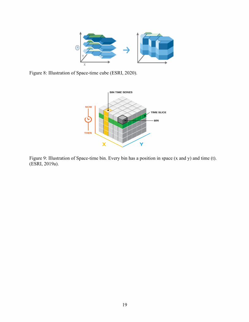
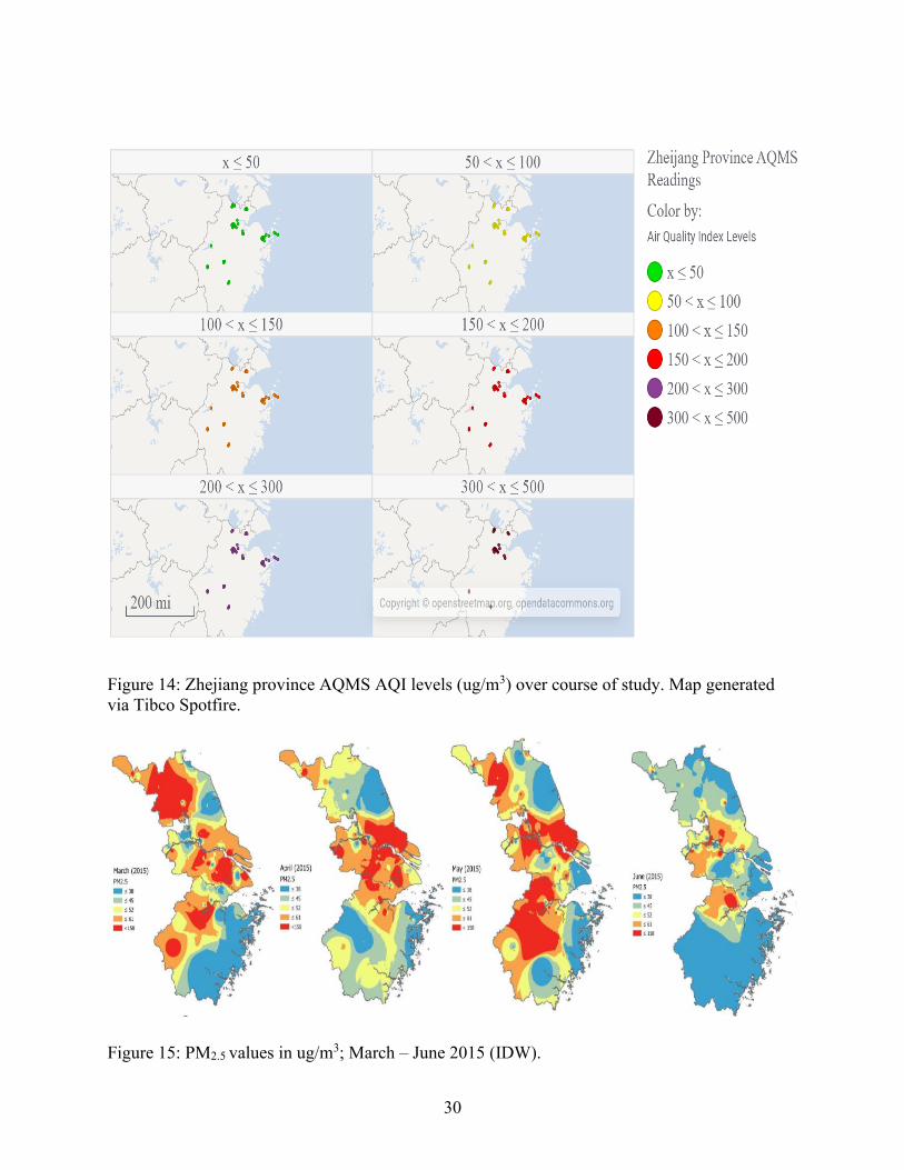
Air quality monitoring stations (AQMS) in Zhejiang province attained AQI levels

ranging from Grade I to Grade VI (Figure 14). All AQMS experienced good (Grade I, 0–50

ug/m3) to very unhealthy (Grade V, 201–300 ug/m3) levels on the AQI. Jinhua, Ningbo, and

Zhoushan were the only cities in Zhejiang province exempted from hazardous (Grade VI, 301-

500 ug/m3) levels. It is important to note that out of the 125 AQMS, 73 are in Jiangsu province

(13 cities), 8 in Shanghai, and 44 in Zhejiang province (9 cities).

22

Inverse Distance Weighted (IDW) Interpolation

The data produced 16 interpolated maps (monthly), showing concentration spread over

the YRD. PM2.5 categories were manually classified by obtaining the average of all IDW values

from the product of quantile classification. The manual classifications are: ≤ 38 ug/m3, ≤ 45

ug/m3, ≤ 52 ug/m3, ≤ 61 ug/m3, and <158 ug/m3. Figure 15 displays the first four months of the

readings (March - June 2015) which portray an interesting spread of PM2.5. During March 2015,

we observe the majority of Jiangsu province, and Shanghai were covered in the highest

interpolated values (61 ug/m3 ≤ x < 158 ug/m3), while only the western part of Zhejiang province

was dominated by the highest interpolated values. In April 2015, the highest interpolated values

transferred to central YRD where the southern Jiangsu, and northern Zhejiang provinces are

located. The highest interpolated values dispersed into May 2015 as it did in March 2015;

however, it accommodated a larger area in Zhejiang. As summer approached, June 2015

generated the lowest interpolated values (≤ 38 ug/m3) through the YRD except along the Yangtze

River where majority of industrialization takes place. In Figure 16, July, August, and September

2015 followed decreasing levels, indicating better air quality in the summer months. However, as

fall approached, the highest interpolated values dominated the central and northern regions of the

YRD. Figure 17 shows that as November 2015 transitioned into the colder months, high PM2.5

levels covered Jiangsu and by December 2015 covered the whole YRD. January 2016 followed

the same pattern, while the eastern parts of Zhejiang started to show signs of lower interpolated

values in February 2016. High interpolated PM2.5 values remained throughout the YRD in March

2016 (Figure 18). As warmer weather surged, the values dramatically dropped through the whole

Zhejiang province during April 2016. By May 2016, the higher interpolated values concentrated

23

in the eastern half of the YRD less than the previous year (March 2015). Like June 2015, the

lower interpolated values dominated June 2016.

Space-Time Pattern Mining

Decreasing trends in PM2.5 concentrations were observed over the study area through the

2D space-time cube visualization (Figure 19). It is important to note that not all stations have the

same downward trend. Most cities on the Yangtze River show a downward trend with a 95%

confidence over time. While in Jiangsu province, most stations in the cities of Nantong and

Suzhou portray 99% confidence in a downward trend. Huzhou and Jiaxing in Zhejiang province

compile of some stations with 99% confidence in a downward trend. Stations 95% and greater in

a downward trend are located near the central region of the YRD. This indicates that PM2.5 levels

have been going down over the study period along the Yangtze River. Figure 20 is the product of

emerging hot spot analysis with the hourly data aggregated in monthly time-step intervals.

AQMS located in the city of Suqian in Jiangsu province produced a sporadic hot spot pattern. In

Zhejiang province, the cities of Shaoxing, Hangzhou, Jinhua, and Quzhou produced an

oscillating hot spot pattern. While Xuzhou was the only city in Jiangsu province with an

oscillating hot spot pattern. AQMS located in the far eastern region of Zhejiang province

produced persistent and sporadic cold spot patterns. All the AQMS in Zhoushan and two AQMS

from Ningbo illustrated persistent cold spot patterns. The other 7 AQMS in Ningbo produced a

sporadic cold spot pattern indicating an on-again then off-again cold spot. The AQMS situated in

cities along the Yangtze River including Zhenjiang, Taizhou, Yangzhou, and Nantong from

Jiangsu province and Shanghai, produced an oscillating cold spot pattern. The AQMS present in

the city of Yancheng in Jiangsu province also produced an oscillating cold spot pattern. The rest

of the AQMS in the YRD did not detect a pattern.

24

Most of the AQMS along the river were oscillating cold spots, with others showing no

pattern. The trend in PM2.5 levels over the study period were expected to be higher due to the

high energy output of coal power stations. However, that was not the case from the space-time

pattern analysis. The northern-eastern city of Xuzhou in Jiangsu province and southern cities of

Hangzhou, Shaoxing, Jinhua, and Quzhou in Zhejiang province were the only cities to present

oscillating hot spot patterns. They are located far from the Yangtze River and these cities in

Zhejiang (3 power stations) oversee less presence of coal power stations contrary to Xuzhou (13

power stations in Jiangsu.

Multiple Linear Regression Analysis

The readings were obtained from AQMS in the YRD over 16 months starting in March

2015 until June 2016. Data for the months of March, April, May, and June (spring-to-summer)

which is ideal for understanding the relationship between GWTC-2 and PM2.5. Tables 3 and 4

examined the weather types in each province and their p-values in relation to PM2.5. The p-values

for the weather types Humid Warm (HW), Warm (W) and Dry Warm (DW) in Jiangsu prove to

be statistically significant (<0.05) at 0.01200, 0.00001 and 0.02278 respectively. For Jiangsu, in

the spring-to-summer months in 2016, only W had a p-value statistically significant at 0.01944.

Statistically significant p-values in Shanghai were only present in 2015. Like Jiangsu, Shanghai

had HW, W, and DW with p-values at 0.05033, 0.00268, and 0.00548 respectively. In contrast,

GWTC-2 weather types in Zhejiang only had statistically significant p-values in 2016 at

0.03418, 0.01851, and 0.00714 for Humid (H), Warm (W) and Cold Front Passage (CFP)

respectively. Figures 21, 22, and 23 illustrate the average PM2.5 present on statistically significant

GWTC-2 classification (H, HW, W, CFP) days during spring-to-summer months in 2015 (orange

25

bar) and spring-to-summer months in 2016 (aqua bar). In Jiangsu and Shanghai, the average

PM2.5 values are higher for each GWTC-2 variable except CFP for Shanghai in 2015 than 2016.

Zhejiang follows a similar trend except for DW where the 2016 average is higher than 2015. In

Jiangsu, presence of HW had an average PM2.5 reading of 53 ug/m3 (7 days), W at 72.4 ug/m3 (11

days) and DW at 58.6 ug/m3 (5 days) in the spring-to-summer months in 2015, while W was at

63 ug/m3 (8 days) in the spring-to-summer months in 2016. Similarly, in Shanghai HW had an

average reading of 53.2 ug/m3 (8 days), W at 67.9 ug/m3 (14 days), and DW at 68.8 ug/m3 (5

days) during spring-to-summer in 2015. In contrast, Zhejiang portrayed a strong relationship

between H, W, and CFP, while the average PM2.5 readings were lower than Jiangsu and Shanghai

during the spring-to-summer months 2016. Humid weather type occupied 26 days with an

average PM2.5 reading of 35 ug/m3, Warm at 32.8 ug/m3 (17 days), and CFP at 22.5 ug/m3 (3

days). More information regarding other GWTC-2 weather types in Jiangsu, Shanghai, and

Zhejiang are present in Appendix B-1, B-2, B-3, B-4, B-5, and B-6.

26

GWTC-2 Classification Jiangsu Shanghai Zhejiang

Humid Warm (HW) 0.01200 0.05034 0.26014

Warm (W) 0.00001 0.00268 0.09869

Dry Warm (DW) 0.02278 0.00548 0.18259

Humid (H) N/A N/A 0.13735

Cold Front Passage (CFP) 0.433058 0.09012 0.54079

GWTC-2 Classification Jiangsu Shanghai Zhejiang

Humid Warm (HW) 0.06433 0.95817 0.07458

Warm (W) 0.01944 0.28070 0.01851

Dry Warm (DW) 0.15646 0.93892 0.17427

Humid (H) 0.16580 0.79515 0.03418

Cold Front Passage (CFP) 0.20359 0.53160 0.00714

Table 4. Multiple linear regression p-value summary table for statistically significant GWTC-2

variables during March, April, May, and June (2016) for Jiangsu, Shanghai, and Zhejiang.

Table 3. Multiple linear regression p-value summary table for statistically significant GWTC-2

variables during March, April, May, and June (2015) for Jiangsu, Shanghai, and Zhejiang.

27

Figure 10: Monthly mean PM2.5 (x-axis) for (a) Jiangsu, (b) Shanghai, (c) Zhejiang. All averages

in ug/m3. AQMS recording period on y-axis. Produced using TIBCO Spotfire.

a)

b)

c)

28

a)

b)

c)

Figure 11: Monthly PM2.5 readings (x-axis) for (a) Jiangsu, (b) Shanghai, (c) Zhejiang. All

readings in ug/m3. AQMS recording period on y-axis. Produced using TIBCO Spotfire.

29

Figure 12: Jiangsu province AQMS AQI levels (ug/m3) over course of study. Map generated via

Tibco Spotfire.

Figure 13: Shanghai municipal AQMS AQI levels (ug/m3) over course of study. Map generated

via Tibco Spotfire.

30

Figure 14: Zhejiang province AQMS AQI levels (ug/m3) over course of study. Map generated

via Tibco Spotfire.

Figure 15: PM2.5 values in ug/m3; March – June 2015 (IDW).

31

Figure 16: PM2.5 values in ug/m3; July – October 2015 (IDW).

Figure 17: PM2.5 values in ug/m3; November, December 2015, January and February 2016 (IDW).

Figure 18: PM2.5 values in ug/m3; March – June 2016 (IDW).

32

Figure 19: Visualizing time cube in 2D. Displays trend over time; visible decreasing trend over

time around the Yangtze River. Product of space-time cube created through space-time pattern

mining on ArcGISPro.

33

Figure 20: Emerging hot spot analysis. Displays pattern over time (aggregated monthly); Product

of space-time cube created through space-time pattern mining on ArcGISPro.

34

0

20

40

60

80

H HW DW W CFP

ug/

m3

Shanghai

Avg. PM2.5 (2015) Avg. PM2.5 (2016)

Figure 21: Average PM2.5 in Shanghai on days H, HW, DW, W, CFP are present.

0

20

40

60

80

H HW DW S W CFP

ug/m

3

Zhejiang

Avg. PM2.5 (2015) Avg. PM2.5 (2016)

Figure 22: Average PM2.5 in Zhejiang on days H, HW, DW, W, CFP are present.

0

20

40

60

80

H HW DW W CFP

ug/

m3

Jiangsu

Avg. PM2.5 (2015) Avg. PM2.5 (2016)

Figure 23: Average PM2.5 in Jiangsu on days H, HW, DW, W, CFP are present.

35

DISCUSSION

Using ambient air readings collected at the AQMS in YRD, this study investigated the

trends and distribution of PM2.5 using TIBCO Spotfire, IDW interpolation, and space-time

pattern analysis. IDW interpolation (Figure 17) demonstrated that PM2.5 levels are elevated

highest in the winter months of December 2015, January 2016, and February 2016. This finding

is unsurprising given the regularity of temperature inversions, intensified anthropogenic

emissions from coal combustion, and biomass burning during the winter months (Zhang & Cao,

2015). The interpolated surface portrays Zhejiang to have lower values in comparison to Jiangsu

and Shanghai. These are affected not only by the spread of the AQMS in the southern cities in

the YRD but by meteorological factors and locations of operating coal power stations. The

uneven distribution of AQMS throughout the YRD could have resulted in a decreased quality of

the interpolated result as the maximum and minimum values only occurred at the AQMS

(Gimond, 2019).

The 2D visualization of the space-time cube showed that over the study period there is a

downward trend in the PM2.5 concentration in 20 cities out of the 23 considered in the study area.

Nearly all the AQMS along the Yangtze River portray a downward trend. This is further

strengthened by the output of the emerging hot spot analysis. Most of the AQMS along the river

show oscillating cold spots, while others see no pattern. The cities of Ningbo and Zhoushan

AQMS observed persistent and oscillating cold spot patterns indicating low levels of PM2.5. Over

time, the overall trend in PM2.5 levels was expected to be higher due to the high annual energy

output of the coal power stations. However, as observed in the space-time pattern analysis, that is

not the case in this study. According to Xu et. al (2018), precipitation, wind speed, and relative

36

humidity have major influences on the removal or accumulation of air pollutants any of which

could be contributing factors in the observed decrease of PM2.5 concentrations. Furthermore, the

policies enacted by local governments could also be contributing to this downward trend. In

contrast, a few cities (Hangzhou, Shaoxing, Jinhua, and Quzhou) in Zhejiang province and

Xuzhou in Jiangsu showed an oscillating hot spot pattern indicating a rise in PM2.5 levels in the

last month. While only the city of Suqian in Jiangsu displayed a sporadic hot spot pattern.

Furthermore, being in a marine subtropical climate, the YRD is expected to have received lots of

annual rainfall during the study period; however, data limitations made it impossible to consider

precipitation into the analysis.

A multiple linear regression analysis between GWTC-2 weather types and average daily

PM2.5 readings in March, April, May, and June 2015 and 2016 determined the effect of HW, W,

and DW weather on PM2.5 in Jiangsu and Shanghai in the spring-to-summer months of 2015 as

well as W for Jiangsu in the spring-to-summer months of 2016. In Zhejiang, W, H, and CFP

weather influenced PM2.5 during March, April, May, and June of 2016. In the spring-to-summer

months, these weather types influenced the product of the space-time pattern analysis in the

oscillating hot spot and cold spot patterns. This study shows a connection between GWTC-2

weather types and PM2.5; however further study with multiple years of data is needed to

understand the seasonal effect of these weather types on particle pollution.

The main drawback of this study is that the PM2.5 readings were limited to only 16

months of data. Multiple years of data would help to understand the seasonal effects on PM2.5

longitudinally, but this study provides an essential first step in long-term monitoring and

research. The data on the energy output from the operating power stations in YRD was

insufficient, as it was only available annually. For an in-depth seasonal analysis of coal energy

37

output and PM2.5 concentration, more specific data would be required. In this study, precipitation

data was not considered due to data unavailability. Future studies could include wind speed,

relative humidity, precipitation, monthly coal power stations energy output, and other

anthropogenic sources data, allowing for a principal component analysis (PCA) to better

understand the problem of PM2.5 in the YRD.

The latest Air Laws in China are a sign of progress; however, the implementation is

likely to fall short as the enforcement of these laws is weak (King, 2016). The responsibility of

environmental protection in China is assigned to multiple agencies with overlapping mandates,

hindering the enforcement of environmental law (Zhang & Cao, 2015). Another part of the

problem is that most of the work of environmental protection is done locally, with the national

government given limited authority. While the Ministry of Environmental Protection (MEP) can

give guidance to local environmental protection bureaus, its actual power over them is weak.

This is a problem because local governments are often more concerned with economic growth

than with the environment, and polluting companies are often key generators of local economic

activity (King, 2016). Corruption plays a massive role as Chinese officials have been known to

take bribes from companies in exchange for ignoring violations (Huang, 2015). While China’s

anti-corruption efforts may help to stop such wrongdoings, the problem is likely to continue.

Furthermore, China needs to reduce its coal power capacity by 40 percent over the next decade,

to meet its climate goal stipulated in the Paris Agreement (Oberhaus, 2019). China is the world’s

leader in the manufacture of clean energy industrial components. as it produces the most solar

panels, wind turbines, batteries, and electric vehicles (REN21, 2019). China prioritized pollution

control from the 17 Sustainable Development Goals (SDGs) adopted by the United Nations to

meet its climate goal set forth in the Paris Agreement (UNDP, 2015). If China can shift its

38

demand for coal energy to sustainable energy, China can sustain a healthy and stable long-term

economic growth.

39

CONCLUSIONS

This study investigated ambient air readings recorded at 125 AQMS throughout the YRD

region, examining trends and distribution of PM2.5 using TIBCO Spotfire, IDW interpolation, and

space-time pattern analysis. The results from TIBCO Spotfire, IDW interpolation, and space-

time pattern analysis demonstrated that trends in PM2.5 went down during the period of study.

Furthermore, the multiple linear regression determined that HW, W, DW weather types affected

the PM2.5 levels in Jiangsu and Shanghai during March, April, May, and June 2015. While

during March, April, May, and June 2016 only W effected declining PM2.5 levels in Jiangsu and

W, DW, and CFP in Zhejiang.

Understanding the spatial and temporal nature of PM2.5 emissions, policymakers in China

must look to sectoral pathways that shift energy demand, implement power market reforms, act

on new clean energy technology, and engage provincial leaders in a new investment approach

(Layke, 2019). The findings of this research can serve basis for local governments in the YRD

region to rethink their policy strategies by avoiding future coal powerplant development,

implementing stronger Air Laws, levying fines for polluters, and lead the country towards a

cleaner and more sustainable future.

40

REFERENCES

Arita, A., & Costa, M. (2011). Environmental agents and epigenetics. Handbook of epigenetics

459-476. https://doi.org/10.1016/B978-0-12-375709-8.00028-9

Ayash, T., Gong, S., & Jia, C. Q. (2009). Understanding the climatic effects of aerosols:

Modeling radiative effects of aerosols. ACS symposium series, 149-166.

https://doi:10.1021/bk-2009-1005.ch010

Boucher, O., Randall, D., Artaxo, P., Bretherton, C., Feingold, G., Forster, P., & Zhang, X.-Y.

(2013). Clouds and aerosols. Climate change 2013: The physical science basis.

Contribution of working Group I to the Fifth Assessment Report of the Intergovernmental

Panel on climate change [Stocker, T.F., D. Qin, G.-K. Plattner, M. Tignor, S.K. Allen, J.

Boschung, A. Nauels, Y. Xia. https://doi.org/10.1017/CBO9781107415324.016

Brook, R. D., Rajagopalan, S., Pope, C. A., Brook, J. R., Bhatnagar, A., Diez-Roux, A. V., &

Kaufman, J. D. (2010). Particulate matter air pollution and cardiovascular disease: An

update to the scientific statement from the american heart association. Circulation, 121(21),

2331–2378. https://doi.org/10.1161/CIR.0b013e3181dbece1

Cesaroni, G., Forastiere, F., Stafoggia, M., Andersen, Z. J., Badaloni, C., Beelen, R., & Peters,

A. (2014). Long term exposure to ambient air pollution and incidence of acute coronary

events: Prospective cohort study and meta-analysis in 11 european cohorts from the escape

project. BMJ (Online), 348(January), 1–16. https://doi.org/10.1136/bmj.f7412

Charlson, R. J., Schwartz, S. E., Hales, J. M., Cess, R. D., Coakley, J. A., Hansen, J. E., &

Hofmann, D. J. (1992). Climate forcing by anthropogenic aerosols. Science,255, 423–430,

https://doi:10.1126/science.255.5043.423.

China National Bureau of Statistics. (2018). China statistical yearbook 2018.

https://www.stats.gov.cn/tjsj/ndsj/2018/indexeh.htm

China Power Project. (2016). How is China's energy footprint changing? Retrieved from

https://chinapower.csis.org/energy-footprint/

Clean Air Alliance of China (CAAC). (2013). Air Pollution Prevention and Control Action

Plan. Retrieved from http://en.cleanairchina.org/file/loadFile/26.html

Morrison, W.M. (2019). China's economic rise: History, trends, challenges, and implications

for the United States. Congressional Research Service.

https://www.everycrsreport.com/files/20190625_RL33534_088c5467dd11365dd4ab5f7

2133db289fa10030f.pdf

EPA. (2009a). Integrated Science Assessment (ISA) for particulate matter (Final report, Dec

41

2009). https://cfpub.epa.gov/ncea/risk/recordisplay.cfm?deid=216546

EPA. (2009b). Air quality index (AQI) basics. Retrieved from

https://cfpub.epa.gov/airnow/index.cfm?action=aqibasics.aqi

EPA. (2016). Health and environmental effects of particulate matter (PM). Retrieved from

https://www.epa.gov/pm-pollution/health-and-environmental-effects-particulate-matter-

pm

EPA. (2019). Health and environmental effects of particulate matter ( PM ) Health effects

visibility impairment further reading. 1–2. https://www.epa.gov/pm-pollution/health-and-

environmental-effects-particulate-matter-pm

Erickson, A. C., & Arbour, L. (2014). The shared pathoetiological effects of particulate air

pollution and the social environment on fetal-placental development. Journal of

Environmental and Public Health, 2014. https://doi.org/10.1155/2014/901017

ESRI. (2016). An overview of the interpolation toolset. Retrieved from

https://desktop.arcgis.com/en/arcmap/10.3/tools/spatial-analyst-toolbox/an-overview-of-

the-interpolation-tools.htm

ESRI. (2019a). Emerging hot spot analysis—ArcGIS. Retrieved from

https://pro.arcgis.com/en/pro-app/tool-reference/space-time-pattern-

mining/emerginghotspots.htm

ESRI. (2019b). An overview of the space-time pattern mining toolbox. Retrieved from

https://pro.arcgis.com/en/pro-app/tool-reference/space-time-pattern-mining/an-

overview-of-the-space-time-pattern-mining-toolbox.htm

ESRI. (2020). Create space time cube from defined locations (Space time pattern mining).

https://pro.arcgis.com/en/pro-app/tool-reference/space-time-pattern-

mining/createcubefromdefinedlocations.htm

Gimond. (2019). Spatial analysis (Interpolation). Retrieved from

https://docs.qgis.org/2.18/en/docs/gentle_gis_introduction/spatial_analysis_interpolatio

n.html#figure-idw-interpolation

Global Energy Monitor. (2020). Retrieved from https://globalenergymonitor.org/coal/global-

coal-plant-tracker/

Greanpeace China. (2018). Greenpeace released the 2017 ranking of PM2.5 concentrations

in 365 cities in China: "Atmospheric Ten" goal completed, national ozone pollution and

air management in non-Beijing-Tianjin-Hebei areas need to be strengthened. Retrieved

from https://www.greenpeace.org.cn/air-pollution-2017-city-ranking/andprev=search

Gu, C., Hu, L., Zhang, X., Wang, X., & Guo, J. (2011). Climate change and urbanization in the

42

Yangtze River Delta q. Habitat International, 1–9.

https://doi.org/10.1016/j.habitatint.2011.03.002

Huang, Y. (2015). The truth about Chinese corruption. Retrieved from

https://carnegieendowment.org/2015/05/29/truth-about-chinese-corruption-pub-60265

Hussey, S. J. K., Purves, J., Allcock, N., Fernandes, V. E., Monks, P. S., Ketley, J. M., &

Morrissey, J. A. (2017). Air pollution alters Staphylococcus aureus and Streptococcus

pneumoniae biofilms, antibiotic tolerance and colonisation. Environmental Microbiology,

19(5), 1868–1880. https://doi.org/10.1111/1462-2920.13686

International Trade Administration. (2014). Fact sheets: YRD. Retrieved from

https://2016.export.gov/china/build/groups/public/@bg_cn/documents/webcontent/bg_c

n_075985.pdf

Jakowiuk, A., Urbański, P., Świstowski, E., Machaj, B., & Pieńkos, J. (2008). Meteorological

features of a beta absorption particulate air monitor operating with wireless

communication system. 53, 37–42.

http://www.nukleonika.pl/www/back/full/vol53_2008/v53s2p037f.pdf

Jin, L., Luo, X., Fu, P., & Li, X. (2017). Airborne particulate matter pollution in urban China: A

chemical mixture perspective from sources to impacts. National Science Review, 4, 593–

610. https://doi.org/10.1093/nsr/nww079

Kalisa, E., Archer, S., Nagato, E., Bizuru, E., Lee, K., Tang, N., Pointing, S., Hayakawa, K., &

Lacap-Bugler, D. (2019). Chemical and Biological Components of Urban Aerosols in

Africa: Current Status and Knowledge Gaps. International journal of environmental

research and public health, 16(6), 941. https://doi.org/10.3390/ijerph16060941

King. (2016). Why China's tougher environmental laws are likely to fail. Retrieved from

https://intpolicydigest.org/2016/11/03/china-s-tougher-environmental-laws-likely-fail/

Krewski, D., Jerret, M., Burnett, R. T., Ma, R., Hughes, E., Shi, Y., & J.Thun, M. (2009).

Extended follow-up and spatial analysis of the American Cancer Society study linking

particulate air pollution and mortality. Health Effects Institute,140.

https://www.healtheffects.org/system/files/Krewski140.pdf

Krishna, R. K., Panicker, A. S., Yusuf, A. M., & Ullah, B. G. (2018). On the contribution of

PM2.5 to direct radiative forcing over two urban environments in India. Aerosol Air Qual.

Res. 19: 399-410. https://doi.org/10.4209/aaqr.2018.04.0128

Lee, C. C. (2015a). A systematic evaluation of the lagged effects of spatiotemporally relative

surface weather types on wintertime cardiovascular-related mortality across 19 US cities.

International Journal of Biometeorology, 59(11), 1633–1645.

https://doi.org/10.1007/s00484-015-0970-5

43

Lee, C. C. (2015b). The development of a gridded weather typing classification scheme. 659,

641–659. https://doi.org/10.1002/joc.4010

Lee, P.-C., O.Talbott, E., M. Roberts, J., M. Catov, J., A. Bilonick, R., A. Stone, R., & Ritz, B.

(2012). Ambient air pollution exposure and blood pressure changes during pregnancy. NIH-

PA, 23(1), 1–7. https://doi.org/10.1038/jid.2014.371

Library of Congress (LOC). (2018). Regulation of air pollution. Retrieved from

https://www.loc.gov/law/help/air-pollution/china.php

Lim, S. S., Vos, T., Flaxman, A. D., Danaei, G., Shibuya, K., Adair-Rohani, H., & Ezzati, M.

(2012). A comparative risk assessment of burden of disease and injury attributable to 67

risk factors and risk factor clusters in 21 regions, 1990–2010: a systematic analysis for the

Global Burden of Disease Study 2010. The Lancet, 380 (9859), 2224–2260.

https://doi.org/https://doi.org/10.1016/S0140-6736(12)61766-8

Mesinger, F., Dimego, G., Oceanic, N., & Mitchell, K. (2006). North American regional re-

analysis. Bull. Amer. Meteor. Soc., 87 (3), 343-360. https://doi.org/10.1175/BAMS-87-3-

343

Mining-Technology. (2014). Coal giants: The world’s biggest coal producing countries.

Retrieved from https://www.mining-technology.com/features/featurecoal-giants-the-

worlds-biggest-coal-producing-countries-4186363/

Mohapatra, K., & Biswal, S. . (2014). Effect of particulate matter (PM) on plants , climate ,

ecosystem, and human health. International Journal Fof Advanced Technology in

Engineering and Science, 2(04), 118–129.

http://ijates.com/images/short_pdf/1404370755_P118-129.pdf

Nagpure, A. S., Gurjar, B. R., & Martel, J. (2014). Human health risks in national capital

territory of Delhi due to air pollution. Atmospheric Pollution Research, 5(3), 371–380.

https://doi.org/10.5094/apr.2014.043

National Bureau of Statistics of China. (2018). Retrieved from https://www.stats.gov.cn/english/

Nawrot, T. S., Perez, L., Künzli, N., Munters, E., & Nemery, B. (2011). Public health importance

of triggers of myocardial infarction: A comparative risk assessment. The Lancet, 377(9767),

732–740. https://doi.org/10.1016/S0140-6736(10)62296-9

Nguyen. (2018). How does acid rain affect buildings and statues? Retrieved from

https://sciencing.com/acid-rain-affect-buildings-statues-22062.html

Oberhaus, D. (2019). China is still building an insane number of new coal plants. Retrieved from

https://www.wired.com/story/china-is-still-building-an-insane-number-of-new-coal-plants

Patashnick, H., & Rupprecht, E. G. (1991). Continuous PM10 measurements using the tapered

44

element oscillating microbalance. Journal of the Air and Waste Management Association,

41(8), 1079–1083. https://doi.org/10.1080/10473289.1991.10466903

Pope III, C. A., Burnett, R. T., Thun, M. J., Calle, E. E., Krewski, D., & Thurston, G. D. (2002).

Lung cancer, cardiopulmonary mortality, and long-term exposure to fine particulate air

pollution. The Journal of the American Medical Association, 287(9), 1132–1141.

https://doi.org/10.1001/jama.287.9.1132

Pui, D. Y. H., Chen, S.-C., & Zuo, Z. (2014). PM2.5 in China: Measurements, sources, visibility

and health effects, and mitigation. Particuology, 13, 1–26.

https://doi.org/https://doi.org/10.1016/j.partic.2013.11.001

Rahman, I., & MacNee, W. (1996). Role of oxidants/antioxidants in smoking-induced lung

diseases. Free Radical Biology and Medicine, 21(5), 669–681.

https://doi.org/https://doi.org/10.1016/0891-5849(96)00155-4

REN21. (2019). Global status report. https://www.ren21.net/wp

content/uploads/2019/05/gsr_2019_full_report_en.pdf

Richard, D., Fintan, H., Sally, J. L., David, S., Leonor, T., & Leendart, van B. (2006). Health

risks of PM from long-range transboundary air pollution.

Samoli, E., Peng, R., Ramsay, T., Pipikou, M., Touloumi, G., Dominici, F., & Katsouyanni, K.

(2008). Acute effects of ambient particulate matter on mortality in Europe and North

America : Results from the APHENA study. 1480(11), 1480–1486.

https://doi.org/10.1289/ehp.11345

Schwartz, J. (2000). Harvesting and long term exposure effects in the relation between air

pollution and mortality. 151(5), 440–448.

https://doi.org/10.1093/oxfordjournals.aje.a010228

Seddon, J., Contrerars, S., & Elliot, B. (2019). 5 under-recognized impacts of air pollution.

World Resources Institute. https://www.wri.org/blog/2019/06/5-under-recognized-impacts-

air-pollution

Shanghai Expo. (2020). Exhibition economy and development of the Yangtze River Delta.

Retrieved from https://www.encyclopedia.com/electronics/international-

magazines/exhibition-economy-and-development-yangtze-river-delta

She, Q., Peng, X., Xu, Q., Long, L., Wei, N., Liu, M., & Zhou, T. (2017). Air quality and its

response to satellite-derived urban form in the Yangtze River Delta, China. Ecological

Indicators, 75(November), 297–306. https://doi.org/10.1016/j.ecolind.2016.12.045

Shu, L., Xie, M., Gao, D., Wang, T., Fang, D., Liu, Q., & Peng, L. (2017). Regional severe

particle pollution and its association with synoptic weather patterns in the Yangtze River

Delta region , China. 12871–12891. https://doi.org/10.5194/acp-17-12871-2017

45

Textor. (2020). GDP of Jiangsu, Shanghai, Zhejiang. Retrieved from

https://www.statista.com/statistics/1070331/china-gdp-of-

jiangsu/;https://www.statista.com/statistics/802355/china-gdp-of-

shanghai/;https://www.statista.com/statistics/1092992/china-gross-domestic-product-of-

zhejiang-province/

Tobler, W. (1970). A computer movie simulating urban growth in the Detroit region.

Economic Geography, 46, 234-240. https://doi:10.2307/143141

Tooele County Health Department (TCHD). (2016). Winter inversions. Retrieved from

https://tooelehealth.org/winter-inversions/

Twomey, S. (1974). Pollution and the planetary albedo. Atmospheric Environment (1967), 8(12),

1251–1256. https://doi.org/https://doi.org/10.1016/0004-6981(74)90004-3

UNDP. (2015). SDGs in China. https://www.cn.undp.org/content/china/en/home.html

WHO. (2009). Global health risks: Mortality and burden of disease attributable to selected major

risks. Epidemiology and Statistics. https://apps.who.int/iris/handle/10665/44203

William, M. H., & William R. B. (2004). Evaluating the contribution of PM2.5 precursor gases

and re-entrained road emissions to mobile source PM2.5 particulate matter emissions.

https://www3.epa.gov/ttnchie1/conference/ei13/mobile/hodan.pdf

Wong, D. W., Yuan, L., & Perlin, S. A. (2004). Comparison of spatial interpolation methods for

the estimation of air quality data. Journal of Exposure Analysis and Environmental

Epidemiology, 14(5), 404–415. https://doi.org/10.1038/sj.jea.7500338

Xing, Y., Xu, Y., Shi, M., & Lian, Y. (2016). The impact of PM2.5 on the human respiratory

system. 8(I), 69–74. https://doi.org/10.3978/j.issn.2072-1439.2016.01.19

Xu, Y., Xue, W., Lei, Y., Zhao, Y., Cheng, S., & Ren, Z. (2018). Impact of meteorological

conditions on PM2.5 pollution in China during Winter.

https://doi.org/10.3390/atmos9110429

Zhang, M., T.Mueller, N., Wang, H., Hon, X., J. Appel, L., & Wang, X. (2018). Maternal

exposure to ambient PM2.5 during pregnany and the risk for high blood pressure in

childhood. 25(3), 289–313. https://doi.org/110.1016/j.bbi.2017.04.008

Zhang, Y. L., & Cao, F. (2015). Fine particulate matter (PM2.5) in China at a city level. Scientific

Reports, 5(2014), 1–12. https://doi.org/10.1038/srep14884

46

APPENDICES

Appendix A: Power Stations (Global Energy Monitor, 2020) – Jiangsu, Shanghai, Zhejiang

Appendix A-1. Number of operating power stations in Jiangsu; city and total power station units

included.

City Number of Operating Power Stations Total Units

Suzhou 20 56

Zhenjiang 13 42

Xuzhou 13 31

Wuxi 7 22

Nantong 3 11

Taizhou 3 9

Yangzhou 3 9

Yancheng 3 6

Linagyungang 3 9

Huaien 3 7

Changzhou 2 4

Nanjing 2 4

Suqian 1 2

Total 76

212

47

Appendix A-2. Number of operating power stations in Shanghai; total power station units

included.

Appendix A-3. Number of operating power stations in Zhejiang; city and total power station

units included.

Number of Power Stations Total Units

8 34

City Number of Operating Power Stations Total Units

Ningbo 8 35

Jiaxing 5 14

Lishui 3 12

Quzhou 2 9

Zhoushan 2 6

Huzhou 2 6

Shaoxing 1 6

Total 23 88

48

Appendix B: GWTC-2 - Jiangsu, Shanghai, Zhejiang

Appendix B-1. The presence of GWTC-2 weather types during March, April, May, and June

(2015) in Jiangsu province; last column has Avg. PM2.5 per weather type calculated.


(2016) in Jiangsu province; last column has Avg. PM2.5 per weather type calculated.

Type Abbreviation # Days Present Avg. PM2.5

Humid Cool HC 12 33.3

Humid H 15 44.5

Humid Warm HW 14 53.0

Cool C 6 33.6

Seasonal S 34 42.6

Warm W 8 63.0

Dry Cool DC 1 19.7

Dry D 8 45.7

Dry Warm DW 1 54.4

Cold Front Passage CFP 3 45.1

Warm Front Passage WFP 0 N/A



Humid H 18 54.0


Cool C 10 34.9

Seasonal S 42 48.7

Warm W 11 72.4

Dry Cool DC 0 N/A

Dry D 8 37.9

Dry Warm DW 5 58.6



49


(2015) in Shanghai; last column has Avg. PM2.5 per weather type calculated.


(2016) in Shanghai; last column has Avg. PM2.5 per weather type calculated.

Spring-to Summer: March, April, May, and June 2016 (Shanghai)



Humid H 17 40.7


Cool C 0 N/A

Seasonal S 39 49.1

Warm W 13 59.5

Dry Cool DC 1 34.8

Dry D 8 58.4

Dry Warm DW 1 37.2





Humid H 19 52.2


Cool C 7 34.5

Seasonal S 37 41.9

Warm W 14 67.9

Dry Cool DC 0 N/A

Dry D 11 38.2

Dry Warm DW 5 68.8



50


(2015) in Zhejiang province; last column has Avg. PM2.5 per weather type calculated.



Humid H 15 42.0


Cool C 9 41.6

Seasonal S 33 39.3

Warm W 17 39.9

Dry Cool DC 1 61.4

Dry D 11 44.8

Dry Warm DW 4 42.6




(2016) in Zhejiang province; last column has Avg. PM2.5 per weather type calculated.



Humid H 26 35.0


Cool C 5 35.9

Seasonal S 35 36.5

Warm W 17 32.8

Dry Cool DC 3 39.0

Dry D 1 52.6

Dry Warm DW 1 66.3



evaluating particulate matter 2.5 in the yangtze river delta

Documents