Contents lists available at ScienceDirect

Dendrochronologia

journal homepage: www.elsevier.com/locate/dendro

Original Article

Evaluating the robustness of three ring-width measurement methods forgrowth release reconstruction

Sybryn L. Maesa,⁎, Astrid Vannoppenb, Jan Altmanc, Jan Van den Bulcked, Guillaume Decocqe,Tom De Mild, Leen Depauwa, Dries Landuyta, Michael P. Perringa,f, Joris Van Ackerd,Margot Vanhellemonta, Kris Verheyena

a Forest & Nature Lab, Ghent University, Geraardsbergsesteenweg 267, BE-9090 Melle-Gontrode, BelgiumbUniversity of Leuven, Division Forest, Nature and Landscape, Department of Earth and Environmental Sciences, Celestijnenlaan 200E, Box 2411, BE-3001 Leuven,Belgiumc Institute of Botany of The Czech Academy of Sciences, Zámek 1, 25243 Průhonice, Czech RepublicdUGCT-Woodlab-UGent, Ghent University, Laboratory of Wood Technology, Department of Forest and Water Management, Coupure Links 653, BE-9000 Gent, Belgiume Ecologie et Dynamique des Systèmes Anthropisés (EDYSAN, FRE 3498 CNRS—UPJV), Jules Verne University of Picardie, Rue des Louvels 1, 80037 Amiens Cédex,Francef School of Biological Sciences, The University of Western Australia, 35 Stirling Highway, Crawley, WA 6009, Australia

A R T I C L E I N F O

Keywords:DendrochronologyRing-width measurementGrowth releaseLintabmeasuRingXCTRing-porousDiffuse-porousDisturbance reconstructionTRADERForest disturbanceHistorical ecologyMethodological evaluation

A B S T R A C T

Growth release analysis on tree rings can be used to validate forest disturbances from the known past or re-construct those beyond the time line or resolution of documentary evidence. Differences in ring-width mea-surements may result in incorrect disturbance reconstruction. Yet, little is known about how growth releasedetection is influenced by the ring-width measurement method. Methodological comparisons mostly do not takeinto account the ultimate objective of the measurements nor their practicalities, such as time consumption orsample preparation. We assessed differences in ring-width measurements between three methods (Lintab,measuRing, and DHXCT), in a ring-porous (Quercus robur) and diffuse-porous (Fagus sylvatica) species, andevaluated whether detection of growth releases was consistent among methods We also comprehensivelycompared the methods, including quantitative and qualitative criteria. Growth releases were consistent amongmethods despite small, but significant differences in ring-width values. The apparent robustness of the methodssuggests that they may be substitutable in future growth release studies, although the highlighted drawbacks andnecessary improvements may advocate combined approaches. Furthermore, we propose an evaluation frame-work for quantitative and qualitative methodological decision-making and advocate the need for similarmethodological comparisons within other fields of dendrochronology.

1. Introduction

Ring-width (RW) series contain highly valuable and versatile in-formation to monitor and understand a variety of natural (e.g. succes-sion dynamics) and anthropogenic (e.g. forest management) processes(Speer, 2010). In dendroecology, growth release analyses allow thedetection of historical forest disturbance events (e.g. Nowacki andAbrams, 1997; Altman et al., 2013). A growth release is an abrupt in-crease in radial growth in a tree which experienced improved light ornutrient conditions after mortality of a neighbouring tree (Oliver andLarson, 1990).

Obtaining reliable RW series is essential in growth release studies,since measurement or crossdating (CD) errors in RW series may give

rise to incorrect disturbance reconstruction (Cook and Kairiukstis,1990; Stokes and Smiley, 1996; Speer, 2010). In literature, three typesof RW measurement methods are often used. First, a measuring stagewhich combines a sliding table with a microscope and software package(e.g. Lintab + TSAP-Win) is considered the conventional method(Stokes and Smiley, 1996). Second, semi-automatic image analysis onscanned digital images has gained interest and popularity thanks toincreased availability and improved performance of affordable Flatbedscanners and software for image analysis (Speer, 2010; Maxwell et al.,2011). Commercial (e.g. CooRecorder) or user-created image analysisprograms (e.g. measuRing, Lara et al., 2015) allow manual or automaticdetection of ring boundaries based on properties of scanned imagessuch as colour or light intensity (Maxwell et al., 2011). Third, semi-

https://doi.org/10.1016/j.dendro.2017.10.005Received 22 May 2017; Received in revised form 28 September 2017; Accepted 20 October 2017

⁎ Corresponding author.E-mail address: Sybryn.Maes@UGent.be (S.L. Maes).

Dendrochronologia 46 (2017) 67–76

Available online 31 October 20171125-7865/ © 2017 Elsevier GmbH. All rights reserved.

MARK

automatic image analysis on micro-focus X-ray computed tomography(XCT)-scanned images is a recent, innovative application for tree-ringanalysis (Okochi et al., 2007; Grabner et al., 2009; Van den Bulckeet al., 2014; De Mil et al., 2016; Vannoppen et al., 2017).

Measurement methods have been compared in terms of accuracy ofthe resulting ring widths (Levanič, 2007; Maxwell et al., 2011; Nuttoet al., 2012; Lara et al., 2015; Arenas-Castro et al., 2015). The majorityof these comparative studies evaluated whether a more recent methodmeasured RWs as accurately as a more conventional method (i.e. the“reference” for accuracy), and thus could substitute the latter.

However, the final objective of the measurements has mostly beenignored. Hence, to date, it remains for example unknown to what extentthe employed method for RW measurement affects growth release re-sults. Yet, it is highly relevant to investigate which methods are (more)robust for certain tree-ring analysis types, and thus might be moresuited to use when performing that type of analysis. Firstly because anincreasing number of available methods currently exist and are beingused, without a thorough understanding of how the measurementmethod used influences the measurements and subsequent tree-ringanalysis. Secondly because the resolution of measurements, for in-stance, might be a bigger issue in dendroclimatological studies (preciseannual dating necessary for linking with climate events) than in growthrelease studies. That is, in growth release analyses, mean growth ratesaround a year of interest are relatively compared along the tree-ringseries to identify growth increases above a critical level, so that theprecise RW values might not be of key importance in the release de-tection process. Also, minor dating errors that can arise from using alower resolution might be less of an issue in growth release analyses,since the timing and duration of a release is often allowed to differ witha number of years and still be considered “the same”. This accounts forthe fact that growth responses of trees following the same disturbancecan be delayed in time as well as differ between trees or even withincores of the same tree (e.g. Copenheaver et al., 2009; Šamonil et al.,2015; Müllerová et al., 2016).

Comparative studies, besides generally ignoring the final measure-ment objective, usually do not consider more practical aspects of themeasurement methods, such as time or cost efficiency, required samplepreparation steps, or the user-friendliness of a method, either (Maxwellet al., 2011; Lara et al., 2015; Arenas-Castro et al., 2015). However,besides resolution, these practical aspects may influence the results aswell, and may be well-worth considering when choosing a method,since there are often important trade-offs involved. For instance, if alarge number of cores has to be measured, greater financial investmentsto use a specific method with a higher time efficiency may be justified.On the other hand, when cost price is a cut-off criterion, scientists mayopt for the method that involves the lowest financial investment, bothin terms of hardware and software as well as salaries. Nevertheless,resolution/accuracy remains a key characteristic to consider, and oneshould not accept a lower accuracy in a method, if this leads to un-reliable measurements and thus compromises inferences drawn fromany estimates.

This study aims to address these knowledge gaps by (i) evaluatingthe robustness of three RW measurement methods with a specific ob-jective in mind, i.e. growth release analyses, and (ii) taking into accountall relevant criteria of the methods involved during this evaluation.Furthermore, anatomical differences in ring visibility are accounted forby performing this assessment for a ring-porous (Quercus robur L.) aswell as a diffuse-porous (Fagus sylvatica L.) hardwood species. An im-portant note concerning our first study objective should be made. Ourevaluation of robustness should not be confused with comparativestudies that assess the accuracy of RW measurements with a newermethod compared to a reference method. Contrastingly, we want toevaluate whether expected differences in RW measurements, measuredwith three methods as commonly implemented, actually lead to dif-ferent results of the ultimate growth release analysis. Therefore, we firstevaluate how large or important these differences are, and next,

whether these differences result in different release detection.

2. Material and methods

2.1. Study area

Increment cores were collected from Quercus robur trees in Skåne (SSweden) and Fagus sylvatica in Lyons-la-forêt (N France). The trees weresampled in 20 × 20 m2 forest plots from the European PASTFORWARDproject (ERC Consolidator Grant; Grant Agreement Number 614839): 9plots in Skåne (55.81°N, 13.58°E, 79 masl), and 10 plots in Lyons-la-forêt (49.44°N, 1.48°E, 149 masl). The climate of the Swedish study siteis temperate/subhumid (mean annual precipitation 550 mm, meanannual temperature 7.6 °C), the French site has a temperate climate(MAP 580 mm, MAT 10.0 °C, WorldClim, 2016).

2.2. Increment cores

We cored dominant trees to extract the longest possible tree-ringseries. In each plot, we sampled two trees (max 14.1 m apart); whileonly one dominant tree was present in two plots in Lyons-la-forêt. Twotrees per plot is a sufficient sample size for reconstructing (past) localdisturbance events based on growth release analyses and historical plotrecords (for the ERC-project PASTFORWARD). From each tree, twoperpendicular cores were taken at breast height to enable crossdating(CD) per tree and to increase the reliability of the detected releases,following Woodall (2008) and Buchanan and Hart (2011). In total, wecollected 72 cores (18 trees of each species, 2 cores per tree), which wasconsidered sufficient for an in-depth methodological evaluation (cf.Maxwell et al., 2011; Nutto et al., 2012; Lara et al., 2015; Arenas-Castroet al., 2015).

2.3. Sample processing

The samples were stored in paper straws. Before the X-rayComputed Tomography (XCT) scanning, the samples were dried for24 h at 103 °C to ensure correct density estimates and then mounted incustom-made cardboard holders which can contain 33 intact cores ofvariable length (De Mil et al., 2016). The cores were scanned in batch at110 μm resolution using NanoWood XCT facility, developed by Woo-dlab in collaboration with XRE (www.xre.be) (Dierick et al., 2014; Vanden Bulcke et al., 2014; De Mil et al., 2016). After reconstruction withthe Octopus Reconstruction software licensed by InsideMatters (www.insidematters.eu), core image extraction, tilt and tangential alignmentof the 3D volumes was done (De Mil et al., 2016). To make the ringsvisible on the Lintab and the Flatbed scans, all cores were unwrappedand planed with a Core Microtome (Gärtner and Nievergelt, 2010). ForF. sylvatica, additional sanding with two grades of sandpaper (320 and400 grit) was needed to facilitate ring boundary demarcation. All coreswere scanned with an Epson Perfection Photo (Flatbed) scanner and the2D core images were cropped from the scanned images using the open-source software package ImageJ (Schindelin et al., 2015). The Lintaband Flatbed measurements were performed at equilibrium moisturecontent (i.e. air-dry) since this is custom procedure when using thesemethods. Table S2 provides a workflow including all steps for the threemethods.

2.4. Ring-width measurements

Ring widths were measured with three different methods: (i) aLintab measuring stage with TSAP-Win software (the “Lintab” method),(ii) Flatbed-scanned image analysis with measuRing in R (“Flatbed”) and(iii) XCT-scanned image analysis with the software program DHXCT inMatlab (“XCT”). These methods differ in (i) resolution, (ii) ring de-marcation procedure, and (iii) fibre structure correction. First, the re-solution was determined for each method as a compromise between

S.L. Maes et al. Dendrochronologia 46 (2017) 67–76

68

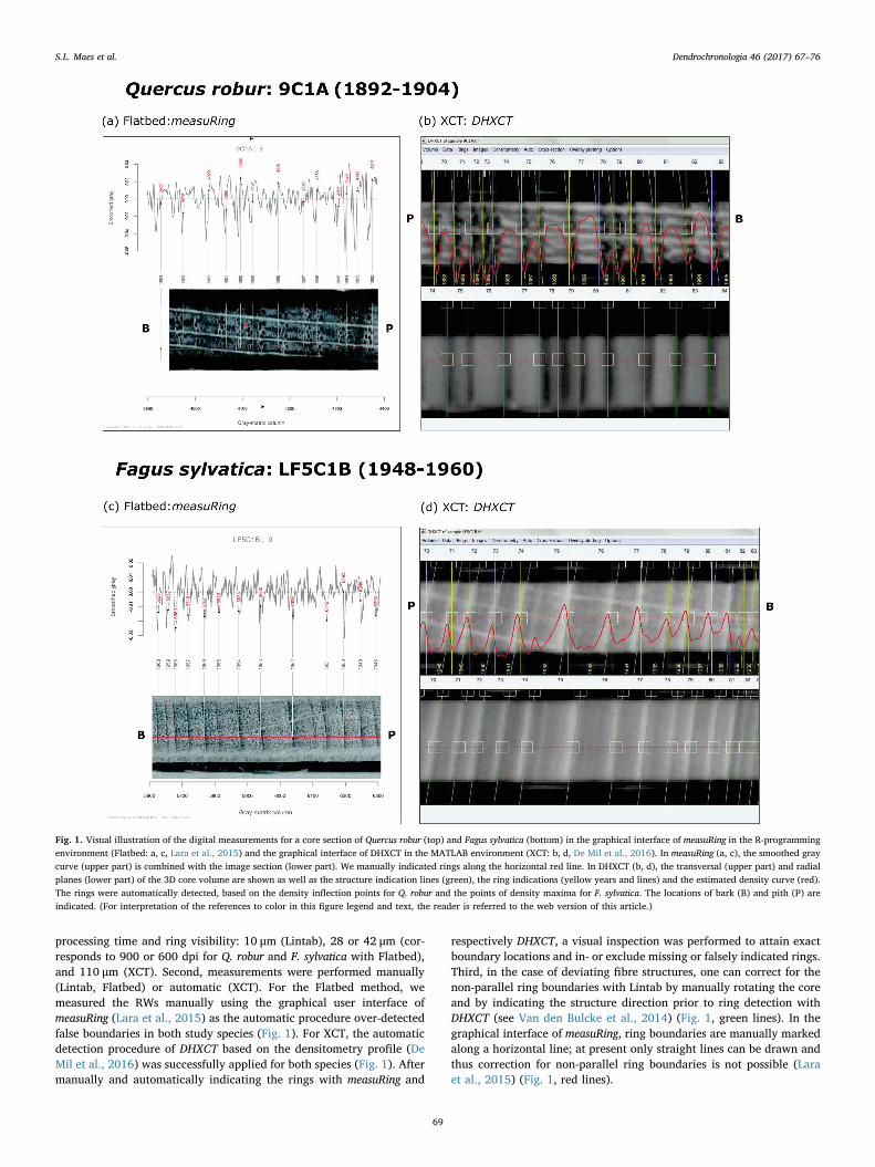
processing time and ring visibility: 10 μm (Lintab), 28 or 42 μm (cor-responds to 900 or 600 dpi for Q. robur and F. sylvatica with Flatbed),and 110 μm (XCT). Second, measurements were performed manually(Lintab, Flatbed) or automatic (XCT). For the Flatbed method, wemeasured the RWs manually using the graphical user interface ofmeasuRing (Lara et al., 2015) as the automatic procedure over-detectedfalse boundaries in both study species (Fig. 1). For XCT, the automaticdetection procedure of DHXCT based on the densitometry profile (DeMil et al., 2016) was successfully applied for both species (Fig. 1). Aftermanually and automatically indicating the rings with measuRing and

respectively DHXCT, a visual inspection was performed to attain exactboundary locations and in- or exclude missing or falsely indicated rings.Third, in the case of deviating fibre structures, one can correct for thenon-parallel ring boundaries with Lintab by manually rotating the coreand by indicating the structure direction prior to ring detection withDHXCT (see Van den Bulcke et al., 2014) (Fig. 1, green lines). In thegraphical interface of measuRing, ring boundaries are manually markedalong a horizontal line; at present only straight lines can be drawn andthus correction for non-parallel ring boundaries is not possible (Laraet al., 2015) (Fig. 1, red lines).

Fig. 1. Visual illustration of the digital measurements for a core section of Quercus robur (top) and Fagus sylvatica (bottom) in the graphical interface of measuRing in the R-programmingenvironment (Flatbed: a, c, Lara et al., 2015) and the graphical interface of DHXCT in the MATLAB environment (XCT: b, d, De Mil et al., 2016). In measuRing (a, c), the smoothed graycurve (upper part) is combined with the image section (lower part). We manually indicated rings along the horizontal red line. In DHXCT (b, d), the transversal (upper part) and radialplanes (lower part) of the 3D core volume are shown as well as the structure indication lines (green), the ring indications (yellow years and lines) and the estimated density curve (red).The rings were automatically detected, based on the density inflection points for Q. robur and the points of density maxima for F. sylvatica. The locations of bark (B) and pith (P) areindicated. (For interpretation of the references to color in this figure legend and text, the reader is referred to the web version of this article.)

S.L. Maes et al. Dendrochronologia 46 (2017) 67–76

69

2.5. Crossdating

To ensure correctly dated tree-ring series, we crossdated the twocores per tree, the four cores per plot and ultimately all cores per studysite. To allow comparison of the results, we performed CD in a similarway for all methods, following a graphical and statistical crossdatingprocedure in TSAP-Win. The CD was considered acceptable if the glei-chläufigkeit (percentage of simultaneous RW increases or decreases,Buras and Wilmking, 2015), CD index (index of possible best matchpositions for two or more series) and t-value after Ballie-Pilcherwere> 65,> 30 and>6 (see Table S1 for CD details). We omittedfour series of Q. robur and four of F. sylvatica with bad CD results due tonarrow and unclear rings from further analyses.

2.6. Data analysis

Because a growth release can be expressed on only one side of thetree (Copenheaver et al., 2009), they are not necessarily detected inboth cores of a sampled tree. Therefore, we performed all furtheranalyses on the individual series and not on average series per tree.

2.6.1. Measurement differencesTo assess the differences in RW measurements among methods,

distributions of all RWs were first graphically and then statisticallycompared by evaluating boxplots and performing two-sampleKolmogorov-Smirnoff tests (ks.test function in R-package “stats”) forboth species (R Development Core Team, 2016).

To reveal systematic methodological biases, the difference in pairedRWs between two methods was plotted against the average of thesepaired RWs (Bland and Altman, 1986, 1999). In these Bland and Altmangraphs, the overall mean RW difference is compared with the equalityline (i.e. zero difference) and the observed RW differences are com-pared with the limits of agreement (mean RW difference± 1.96 timesthe standard deviation of the differences) (Bland and Altman, 1999;Giavarina, 2015; Bland and Altman, 1986). Histograms and QQ plotsdetermined quite heavy-tailed distributions of differences, violating theassumption of normality of differences to calculate the limits ofagreement in a correct way (Bland and Altman, 1999). However, fol-lowing Bland and Altman (1999), this violation is not an issue to in-terpret the plots.

To test for significant differences in RWs among methods, we usedunivariate Repeated Measures ANOVA (factor “method” with 3 levels).To create a sensible sample size to perform this statistical test (the totalS.S. of ca. 3600 RWs resulted in very low p-values, thus always sig-nificant results), 10.000 tests of 32 randomly chosen RWs (one RWmeasurement per core, same measured ring in all methods) were per-formed and the resulting p-value histograms and frequency of sig-nificant results were assessed. At the same time, random selection re-moved any dependencies in the RW data of each method due tointerrelatedness of rings from the same core (i.e. autocorrelation), ofcores from the same tree and cores from the same plot. All assumptionsfor the Repeated Measures ANOVA were evaluated, including normaldata distributions (with QQ plots), homoscedasticity (with variancetests), independence of measurements per method (solved by randomselection) and sphericity (with Mauchly’s test). Mauchly’s test resultswere used to determine per test result whether the sphericity assumedp-value (if Mauchley’s p > 0.05) or the Greenhouse-Geisser correctedp-value (if p < 0.05) reflected the Repeated Measures result (Parket al., 2009).

Finally, to assess which methods were different from each other,post-hoc pairwise comparison tests were performed for each test datasetof the 10.000 replicates for which a significant difference among thethree methods was found. This was done with the function pairwise.t.testusing the Bonferroni correction in R (R Development Core Team, 2016)and both assumptions of normality and homoscedasticity were fulfilled.

2.6.2. Growth release analysesRelease events were determined with Radial Growth Averaging

(RGA), i.e. one of the most common “running mean release identifica-tion” methods using the “TRADER” package (Altman et al., 2014) in R(R Development Core Team, 2016; Rubino and McCarthy, 2004). Thistechnique computes the percentage growth change (%GC) for eachtarget year as %GC = [(M2 − M1)/M1]*100, with M1 and M2 beingthe average radial growth over the preceding and subsequent 10-yearperiod, including (M1) and excluding (M2) the target year (Nowackiand Abrams, 1997). TRADER detects a release as a sustained period ofincreased growth by running comparisons of the sequential%GC values.We selected a 10-year span for the GC calculation since this tends toaverage out short-term growth responses related to climate (Nowackiand Abrams, 1997). Furthermore, a release was only detected if theperiod of increased growth (i) exceeded the threshold of 25%GC and50%GC for a moderate and a major release; (ii) was sustained for atleast seven years; and (iii) if the release was a minimum of ten yearsapart from another detected release. Within a release, or the time periodin which all criteria are fulfilled, TRADER identifies the release year asthe year with the maximum% GC. Since we were interested in whetherrelease detection results would be different among measurementmethods, we used fixed criteria for our analysis.

To examine the differences in release detection observed amongmeasurement methods, we considered differences in magnitude or timingof the observed releases. A difference in magnitude was defined if arelease was detected by one method but not by another, or if a releasewas classified as a major release by one method and moderate by an-other. A difference in timing occurred when the release year differedbetween methods.

2.7. Comprehensive evaluation of the three methods

The following (i) quantitative and (ii) qualitative criteria wereevaluated for each method: (i) time consumption, cost, data storage,sample length, RW resolution, and (ii) fibre structure correction, woodanatomy, availability of hard- and software, core destructiveness, coredrying, verifiability/repeatability, added value and user-friendliness. Allcriteria were scored from 1 (best) to 3 (worst) for each method, basedon real values or orders of magnitude for the quantitative criteria andon personal experience for the qualitative ones.

3. Results & discussion

3.1. Measurement differences

The majority of the ring widths measured with the three methodswas quite similar (Figs. 2 and 3), and no method showed an extrememeasurement bias (Fig. 3). However, the ring-width distributions diddiffer significantly between XCT and Flatbed (p < 0.001 for Q. roburand F. sylvatica) and Lintab (p = 0.02, p = 0.005), but not betweenLintab and Flatbed (p = 0.06, p = 0.6). Flatbed also tended to over-estimate ring widths compared to Lintab or XCT for Q. robur (Fig. 3a, c:more outliers below than above the limits of agreement). For bothspecies, RW measurements were smallest with XCT (Figs. 2 and 3),reflected also by the lower median RW of 1.88 and 2.02 mm for Q. roburand F. sylvatica with XCT compared to 1.96 and 2.12 mm with Lintaband 1.99 and 2.14 mm with Flatbed. Although not statistically sig-nificant, Flatbed measured slightly bigger RWs than Lintab in bothspecies (Figs. 2 and 3). Overall, RW measurements increased from XCTto Lintab to Flatbed (Figs. 2 and 3, Table 1).

These differences might be explained by a combination of the fol-lowing factors. First, XCT scanning was performed on oven-dry cores toenable correct density estimates, whereas Lintab and Flatbed mea-surements were performed on cores at equilibrium moisture content. Asa result, a dimensional wood shrinkage factor likely led to narrowerrings in XC Vannoppen et al. (2017), investigating the same study

S.L. Maes et al. Dendrochronologia 46 (2017) 67–76

70

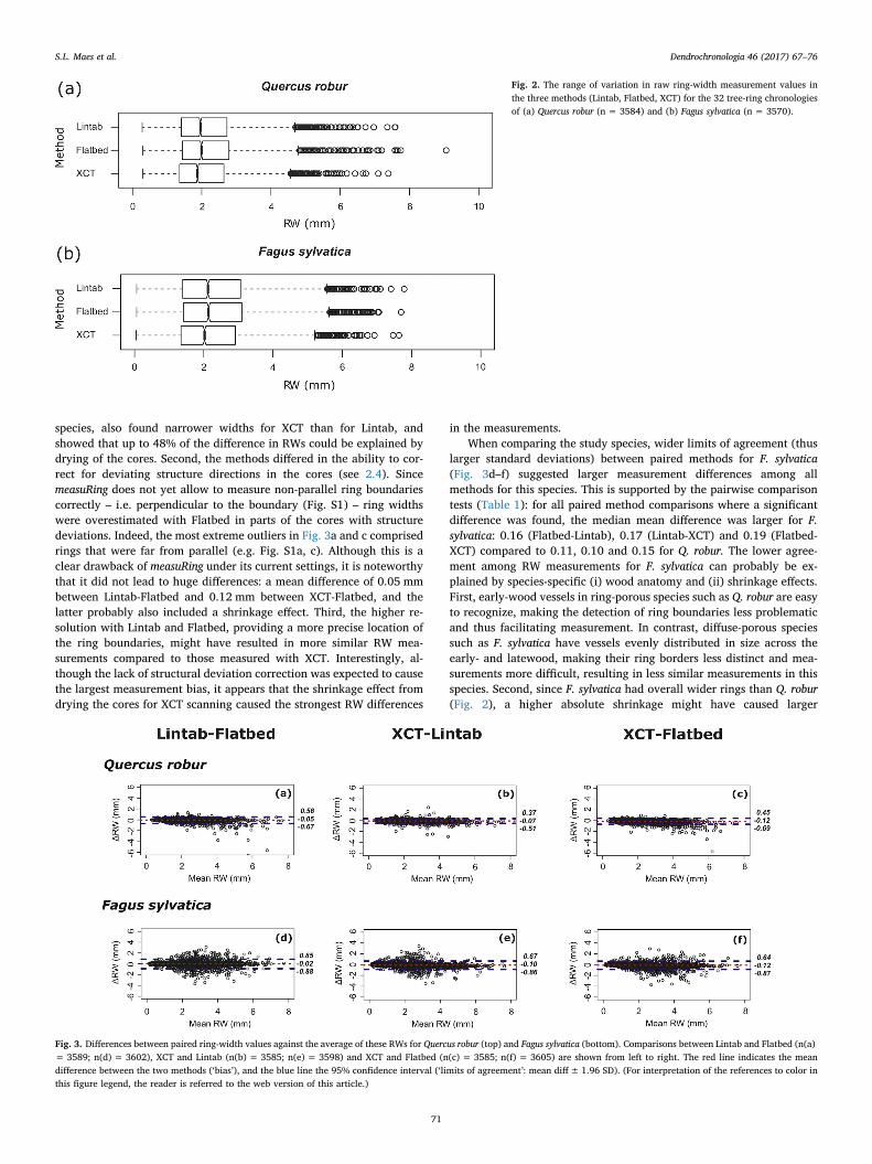
species, also found narrower widths for XCT than for Lintab, andshowed that up to 48% of the difference in RWs could be explained bydrying of the cores. Second, the methods differed in the ability to cor-rect for deviating structure directions in the cores (see 2.4). SincemeasuRing does not yet allow to measure non-parallel ring boundariescorrectly – i.e. perpendicular to the boundary (Fig. S1) – ring widthswere overestimated with Flatbed in parts of the cores with structuredeviations. Indeed, the most extreme outliers in Fig. 3a and c comprisedrings that were far from parallel (e.g. Fig. S1a, c). Although this is aclear drawback of measuRing under its current settings, it is noteworthythat it did not lead to huge differences: a mean difference of 0.05 mmbetween Lintab-Flatbed and 0.12 mm between XCT-Flatbed, and thelatter probably also included a shrinkage effect. Third, the higher re-solution with Lintab and Flatbed, providing a more precise location ofthe ring boundaries, might have resulted in more similar RW mea-surements compared to those measured with XCT. Interestingly, al-though the lack of structural deviation correction was expected to causethe largest measurement bias, it appears that the shrinkage effect fromdrying the cores for XCT scanning caused the strongest RW differences

in the measurements.When comparing the study species, wider limits of agreement (thus

larger standard deviations) between paired methods for F. sylvatica(Fig. 3d–f) suggested larger measurement differences among allmethods for this species. This is supported by the pairwise comparisontests (Table 1): for all paired method comparisons where a significantdifference was found, the median mean difference was larger for F.sylvatica: 0.16 (Flatbed-Lintab), 0.17 (Lintab-XCT) and 0.19 (Flatbed-XCT) compared to 0.11, 0.10 and 0.15 for Q. robur. The lower agree-ment among RW measurements for F. sylvatica can probably be ex-plained by species-specific (i) wood anatomy and (ii) shrinkage effects.First, early-wood vessels in ring-porous species such as Q. robur are easyto recognize, making the detection of ring boundaries less problematicand thus facilitating measurement. In contrast, diffuse-porous speciessuch as F. sylvatica have vessels evenly distributed in size across theearly- and latewood, making their ring borders less distinct and mea-surements more difficult, resulting in less similar measurements in thisspecies. Second, since F. sylvatica had overall wider rings than Q. robur(Fig. 2), a higher absolute shrinkage might have caused larger

Fig. 2. The range of variation in raw ring-width measurement values inthe three methods (Lintab, Flatbed, XCT) for the 32 tree-ring chronologiesof (a) Quercus robur (n = 3584) and (b) Fagus sylvatica (n = 3570).

Fig. 3. Differences between paired ring-width values against the average of these RWs for Quercus robur (top) and Fagus sylvatica (bottom). Comparisons between Lintab and Flatbed (n(a)= 3589; n(d) = 3602), XCT and Lintab (n(b) = 3585; n(e) = 3598) and XCT and Flatbed (n(c) = 3585; n(f) = 3605) are shown from left to right. The red line indicates the meandifference between the two methods (‘bias’), and the blue line the 95% confidence interval (‘limits of agreement’: mean diff±1.96 SD). (For interpretation of the references to color inthis figure legend, the reader is referred to the web version of this article.)

S.L. Maes et al. Dendrochronologia 46 (2017) 67–76

71

differences between XCT and the other methods in this species. This issupported by the higher mean difference between XCT and the othermethods (0.10 mm Lintab, 0.12 mm Flatbed) than between Lintab-Flatbed (0.02 mm) (Fig. 3d–f).

3.2. Growth release analyses

The number of releases detected for Q. robur and F. sylvatica differedslightly among the three methods, for moderate and major releases aswell as the total number of releases, with Lintab and Flatbed more si-milar than XCT (Table 3). This trend agrees with the higher similarity inRW measurements found between Lintab and Flatbed compared tothose from XCT (see 3.1). While the majority of the detected releases inQ. robur were moderate (e.g. 25 moderate, 4 major for XCT), moremajor releases were detected for F. sylvatica (e.g. 23 moderate, 19major) (Table 3).

Even though measurement method did not seem to influence thenumber of releases considerably, the release signals did differ amongthe three methods (Tables 4 and S3). Out of all the releases detected forQ. robur and F. sylvatica, 48 and 59% were equally detected in the seriesfrom the three methods. Of the remaining growth releases, their dif-ference in detection between methods included differences in timing(10 for Q. robur, 8 for F. sylvatica), magnitude (5 Q. robur, 7 F. sylvatica),or both magnitude and timing (3 for F. sylvatica). The majority of thetiming differences was less than 5 years (only 1 out of 21 releases dif-fered with 6 years: Table S3b), and the majority of the magnitude dif-ferences were releases that remained undetected with one or two of thethree methods (9 out of 15 releases: see Table S3b). Only a few releaseswere differently detected with all three methods.

Examining the differences in detail revealed two causes. Differentlengths of the measured tree-ring series caused one magnitude differ-ence; while all others originated from the differences in absolute RWvalues between methods (see Fig. S2 for examples). First, the detectiondifference caused by different lengths of the measured tree-ring series,even though measuring the exact same core, arose because the micro-scopic and scanned images with Lintab and Flatbed were unclear before1899. We could not reliably demarcate ring boundaries with thesemethods anymore before 1899, while the XCT images were clear en-ough to measure until 1880. Because of this, a 1900 release that wasdetected with XCT remained undetected with the other two methods(i.e. the magnitude difference). Of course, measuring different lengthswith a chosen method would not be an issue in a “real” tree-ring studysince one measures only one core, thus creating one tree-series (length).However, this example nicely illustrates a specific advantage of the XCTmethod over Flatbed or Lintab here, related to “how” each methodvisualizes the tree rings. Namely, the XCT measurements are based on3D volumes coupled with density values to aid with tree-ring de-marcation, thus unclear core sections on the 2D volume might still bereliably measured with XCT compared to Lintab or Flatbed. Second, themore frequent differences in detection caused by different RW valuesbetween methods ensued from the subtle differences in calculated

growth change values along the time series leading to variations intiming, number and magnitude of identified releases (Fig. S2). For in-stance, the 1924 release detected with Flatbed and XCT remained un-detected with Lintab because of small differences in absolute measuredvalues resulting in different% growth change values (Fig. S2).Specifically, the growth change was not sustained for long enoughabove the threshold (only 6 years> 25% instead of 7) to be detected asa moderate release by TRADER. Similarly, the 1960 release detectedwith Lintab remained undetected with Flatbed and XCT.

When interpreting the graphical growth release output for all cores,however, all the aforementioned different growth releases amongmethods could be identified as the same releases. Specifically, de-pending on the exact detection technique used for the growth releaseanalysis, these differences could ultimately be interpreted as the sameresults. First, for the timing differences, all but one consisted of a< 5-year difference in release year. If we accept here a buffer of 6 yearsaround the exact timing of a release as is commonly accepted in growthrelease studies, all the differences between measurement methods canbe considered the same. In growth release studies, this timing buffer isused to account for delayed growth responses following a disturbanceevent or variation in individual tree growth (e.g. Šamonil et al., 2015;Müllerová et al., 2016; Copenheaver et al., 2009). Nevertheless, wereason that it is suitable to use this buffer in this context, since we areassessing which releases would ultimately be considered as the result ofindividual disturbance events when interpreting the results for dis-turbance reconstruction. Second, when reassessing the magnitude dif-ferences graphically, we found that these can also be tackled, butthrough a more thorough evaluation of the parameter values during therelease analysis (in TRADER). Here, we used fixed criteria, since wewere primarily interested in whether detection would be differentamong methods. However, changing the criteria to characterize re-leases – a process referred to as adjusting their sensitivity (Altman et al.,2014) – is common in growth release studies and might be appropriatedepending on the study objectives. For instance, by lowering thenumber of years that the growth increase needs to be sustained, onemight detect the “undetected” releases that were graphically visiblewith that method, but just did not reach all fixed criteria. Also, byediting the thresholds for a major or moderate release, one could detectthe releases with a different magnitude. Finally, even with a sensitivityanalysis of the criteria, a visual inspection is recommended after everygrowth release analysis, to estimate the validity of every detected re-lease, as well as to include other, missing releases (Fraver and White,2005).

3.3. Comprehensive evaluation of the three methods

Each method has specific benefits and drawbacks (Table 2). Forinstance, the low data storage requirement for Lintab was a benefit(best score), whereas the difficulty to double-check RW measurementswas a clear drawback (lowest score). The digital workflow of Flatbed,but especially of XCT with its automatic ring detection procedure,

Table 1Post-hoc pairwise comparison tests (Bonferroni correction) for significant differences of RW values among the three methods as determined by Repeated Measures ANOVA (i.e. 7287replicates of Quercus robur and 2771 of Fagus sylvatica).

species Pairwise comparison % significant tests(a) median sign level(b) median mean Δ (mm) interpretation

Quercus robur Lintab-Flatbed 9% * −0.11 Flatbed > LintabXCT-Lintab 39% * −0.10 Lintab > XCTXCT-Flatbed 60% * −0.15 Flatbed > XCT

Fagus sylvatica Lintab-Flatbed 1% * −0.16 Flatbed > LintabXCT-Lintab 15% * −0.17 Lintab > XCTXCT-Flatbed 19% * −0.19 Flatbed > XCT

a i.e. number of significant paired tests/significant repeated measures tests. Note that the sum of these can be> 100 per species since more than one pair can differ significantly withinone three-way difference test.

b ns: p > 0.1, (*): (p < 0.1); *: p < 0.05; **: p < 0.01; ***: p < 0.001.

S.L. Maes et al. Dendrochronologia 46 (2017) 67–76

72

Table 2Comprehensive evaluation of the three measurement methods: Lintab (L), Flatbed (F) and XCT (C). Several quantitative (Type = Q1) and qualitative (Type = Q2) criteria are scored from1 (best) to 3 (lowest) for each method. Quantitative criteria were scored based on real values or orders of magnitude, and qualitative criteria were scored based on personal experience.“Arguments” explains the reasoning behind the scores. The white, light grey and dark grey shading reflects the best, medium and lowest scored method per criterion.

(continued on next page)

S.L. Maes et al. Dendrochronologia 46 (2017) 67–76

73

allowed large sets of cores to be measured in a short time span and theadditional visual back-up was of high value in the post-editing process(good score for time consumption and verifiability). In terms of soft-ware requirements, Flatbed and XCT both scored well, because they use

freely available computer programs. At the same time, however, theexpert knowledge or “learning” time needed to use these programs wasconsidered a drawback (low score for user-friendliness). The time re-quired to measure the RWs of a core was less than half for XCT com-pared with Flatbed for Q. robur (25 vs. 58 min), but the difference wassmaller for F. sylvatica (42 vs. 53 min) (Table S2). This was probablybecause of the more difficult ring recognition in F. sylvatica, more timewas required for the measurements, independent of the method used.

The evaluation of our three methods (Table 2) provides a frame-work for method evaluation, but it remains a snapshot and should bereassessed in the context of other studies. That is, the criteria werescored according to the exact settings of this particular study, but thesescores may change when a different measurement method (e.g. Atrics,Levanič, 2007) or semi-automatic image analysis program (e.g. Co-oRecorder, Cybis Elektronik, 2010) is involved, as well as if technolo-gical advances (e.g. better scanners) or simply other choices (e.g. higherscan resolution) are made. A number of other, proprietary programs

Table 2 (continued)

*XCT: Cost can be lower when building a dedicated tree-ring analysis scanner (Nanowood was built for different purposes).**For both Flatbed and XCT, you could rotate the core or use another scanner (e.g. A3 flatbed) to increase maximum length.***Spatial resolution, i.e. 25.4 [mm/inch]/optical resolution [dpi].****Flatbed and XCT: This depends of course to a large extent on the scanning resolution, which can be increased.

Table 3Summary table of the growth release results using Radial Growth Averaging for releasedetection. Values denote the number of moderate (Mod), major (Maj) and total(Tot = Mod + Maj) releases detected with the three methods in the tree-ring series ofQuercus robur and Fagus sylvatica (Details Table S2).

Method Mod Maj Tot Mod Maj Tot

Quercus robur Fagus sylvatica

Lintab 24 3 27 22 17 39Flatbed 24 3 27 22 17 39XCT 25 4 29 23 19 42

S.L. Maes et al. Dendrochronologia 46 (2017) 67–76

74

such as CooRecorder, which also use semi-automatic image analysis onFlatbed scanned images, do allow correcting for deviating rings. Yet, wedecided to use measuRing because it is open-source (i.e. an R-package (RDevelopment Core Team, 2016)), which is attractive for scientific stu-dies. As another example, the HECTOR scanner (http://www.ugct.ugent.be/instruments.php) allows to scan longer cores (up to 1 m) thanthe NanoWood XCT scanner we used, but requires much longer scan-ning times (Masschaele et al., 2013). Finally, increasing the resolutionof Flatbed or XCT scans might increase the ease of ring boundary re-cognition, but also implies higher costs, longer scanning times as well aslarger data volumes.

3.4. General discussion

In our study, probably a combination of methodological factors –i.e. different sample preparation (drying), different potential to correctfor non-parallel rings and different resolutions used – gave rise to thevariation in RW measurements with the three methods, as hypothe-sized. These results highlight a number of important technical aspectsregarding the accuracy of RW measurements, which should be takeninto account during (preliminary) method evaluation. For instance, theshrinkage effect from drying is usually not taken into considerationduring tree-ring studies, which mainly focus on the year-to-year growthvariability (Latte et al., 2015). However, this caused strong methodo-logical differences in RW measurements in our study as well as in asimilar study by Vannoppen et al. (2017). Tree-ring scientists shouldthus consider this issue in the future. Our results also demonstrated thatmethodological choices should be assessed per study species, i.e. ameasurement method with a higher resolution might be required for F.sylvatica compared to for Q. robur, in order to minimize the potentiallylarger errors that were found.

Next, comparing the growth release results among methods de-monstrated that measurement method in itself did not affect the ulti-mate release results. This suggests that these methods are robust interms of growth release detection, despite their obvious methodologicaldifferences. However, the initially perceived differences in growth re-leases did emphasize the need for a critical interpretation of releaseresults when using a certain method, for instance by a sensitivity ana-lysis of the parameter values defining a release. Also our findingsshould not be interpreted as an advocacy to use lower-resolutionmethods for growth release analysis. Instead, we put forward the ideathat although the use of a certain method may entail a lower resolutionand thus lower RW precision, this does not necessarily imply a badchoice in the case of release analysis.

From this apparent robustness, we suggest that the three methodscould substitute each other in the case of growth release studies, if onecarefully considers the potential measurement biases. This idea mightopen up new perspectives in the domain of dendroecology. For

instance, tree RW datasets that were measured with various methodscould be used within the same growth release analysis if one accepts theidea of measurement substitutability. This could offer opportunities toperform larger-scale data analyses on databases such as theInternational Tree Ring Data Bank. However, two important pointsshould be considered. First, we add that – whenever possible – acombination of methods may be even more useful than a substitution,and at the same time increase reliability of the measurements. It wasclearly shown that every method visualizes cores, hence growth rings inanother way, offering specific benefits and limitations which could beoptimized by combining rather than substituting methods (see Table 2).For instance, measuring a large batch of cores with DHXCT, but usingLintab to measure very narrow ring sections could optimize workflowby combining the higher time efficiency of DHXCT with the higherresolution of Lintab. Second, the idea that measurement methods couldsubstitute each other is proposed here in the case of growth releaseanalysis and should not be generalized for other applications of tree-ring series.

Besides these technical “accuracy” aspects, there are more facets toconsider during the evaluation of a measurement method, which is whywe performed an overall comparison of the three methods. In Table 2,we brought forward a method evaluation framework that might beuseful for future tree-ring studies to determine which method might bemore suitable in order to achieve ones’ study objective. This is relevantsince the barriers to perform tree-ring studies are strongly diminishingbecause of (i) decreasing cost prices of data storage and material, (ii)increasing availability and accessibility of newer, often digitally ad-vanced methods, as well as (iii) increased importance of tree-ring re-cords in scientific studies.

Which method to choose in a particular study will strongly dependon the study context though. For instance, if low cost is crucial, Lintabor Flatbed might be a better option than XCT although the salariesneeded to perform measurements also require consideration. Besidesmore practical criteria such as cost, time consumption, or hardwareavailability, the versatility of a method can also be important. XCTscanning of increment cores provides wood density information in ad-dition to the RW measurements performed on the 3D volumes (Van denBulcke et al., 2014), which might be used in paleoclimatic (e.g. Fritts,1976) or physiological studies (e.g. Koga and Zhang, 2004). From amulti-value perspective, Lintab will generally be the lesser choice, asthe Lintab measuring stage and TSAP-Win software was designed onlyfor measuring RWs. Overall, we recommend that the complete set ofmethod characteristics is important in deciding upon a method anddifferent trade-offs will have to be made in each study design.

3.5. Conclusion

To conclude, our results demonstrated that measurement method in

Table 4Summary table of differences in detected releases in the RW series obtained with Lintab (L), Flatbed (F) and XCT (C) for Quercus robur (top) and Fagus sylvatica (bottom). The number ofequal (Tot=) and different (Tot Δ, L ≠ F = C, F ≠ L = C, C≠ L = F, L≠ F ≠ C) release signals detected among the methods is expressed in absolute numbers and percentage of alldetected release signals (i.e. Tot #). L ≠ F = C implies the different release signal was detected in the Lintab series, but the same signal was detected in the Flatbed and XCT series. Eitherthe release signals differed in magnitude (Δ magnitude), in timing (Δ timing) or in both (Δ magnitude + Δ timing).

Tot # Tot= Tot Δ L ≠ F = C F ≠ L = C C≠ L = F L≠ F ≠ C

Quercus robur29 14 (48%) 15 (52%) 4 (14%) 3 (10%) 6 (21%) 2 (7%)Δ magnitude: 2 (7%) 0 (0%) 3 (11%) 0 (0%)Δ timing: 2 (7%) 3 (11%) 3 (11%) 2 (7%)

Fagus sylvatica44* 26 (59%) 18 (41%) 6 (14%) 2 (5%) 9 (20%)** 1 (2%)Δ magnitude: 2 (5%) 0 (0%) 5 (11%) 0 (0%)Δ timing: 4 (9%) 2 (5%) 2 (5%) 0 (0%)Δ magnitude + Δ timing: 0 (0%) 0 (0%) 2 (5%) 1 (2%)

* = 42 (maximum no. releases detected was with XCT, see Table 3) + 2 (undetected releases with XCT, but detected with Lintab and Flatbed).** Sum of the numbers below will be 21% due to rounding.

S.L. Maes et al. Dendrochronologia 46 (2017) 67–76

75

itself did not affect the ultimate release results, suggesting that thesemethods are robust in terms of growth release detection, despite theirobvious methodological differences. Furthermore, the differences inRW measurements among methods were larger for F. sylvatica than forQ. robur, indicating that methodological choices should be assessed perspecies. For methodological choices in future tree-ring studies, we re-commend that the complete set of method characteristics be con-sidered, including both accuracy as well as more practical aspects suchas time consumption or sample preparation steps.

Finally, more methodological evaluations taking into account thefinal goal of RW measurements would be useful in future studies.Especially since measurements from an increasing number of availablemethods are being used for a variety of analyses without a thoroughunderstanding of how the method, in all its aspects may have influ-enced the RWs and thus the ultimate tree-ring analysis. Furthermore, asthis study focused on release differences caused by differences in theRW measurements and not by differences in dating, future studiesshould evaluate the effect of measurement method on the temporalprecision as well.

Acknowledgements

We thank the European Research Council [ERC Consolidator grantno. 614839: PASTFORWARD] for funding SLM, LD, KV, DL and MP forscientific research and fieldwork involved in this study. AV was sup-ported by FWO [grant no. G.0C96.14N]. JA was supported by the GrantAgency of the Czech Republic [grants no. 14-12262S and 17-07378S]and the long-term research development project no. RVO 67985939.TDM was supported by the Special Research Fund [grant no.BOF.DOC.2014.0037.01] from the University of Ghent. MV and DLwere funded as postdoctoral fellows by FWO-Vlaanderen. We thank Krisand Filip Ceunen, Haben Blondeel and Jorgen Op de Beeck for theirsupport with the fieldwork in Sweden and France. We are also gratefulto Jörg Brunet and Ulf Johansson (Swedish University of AgriculturalSciences) for their help in site selection, fieldwork and compiling his-torical information in Skåne and similarly to Déborah Closset-Kopp,Jérôme Buridant and the Office National des Forêts for their help inLyons-La-Forêt.

Appendix A. Supplementary data

Supplementary data associated with this article can be found, in theonline version, at http://dx.doi.org/10.1016/j.dendro.2017.10.005.

References

Šamonil, P., Kotík, L., Vašíčková, I., 2015. Uncertainty in detecting the disturbance his-tory of forest ecosystems using dendrochronology. Dendrochronologia 35, 51–61.

Altman, J., et al., 2013. Tree-rings mirror management legacy: dramatic response ofstandard oaks to past coppicing in central europe. PLoS One 8 (2), 1–11.

Altman, J., et al., 2014. TRADER: a package for tree ring analysis of disturbance events inR. Dendrochronologia 32, 107–112.

Arenas-Castro, S., Fernandez-Haeger, J., Jordano-Barbudo, D., 2015. A method for tree-ring analysis using DIVA-GIS freeware. Tree-Ring Res. 71 (2), 118–129.

Bland, J.M., Altman, D.G., 1986. Statistical methods for assessing agreement between twomethods of clinical measurement. Lancet 1 (1), 307–310.

Bland, J.M., Altman, D.G., 1999. Measuring agreement in method comparison studies.Stat. Methods Med. Res. 8 (2), 135–160.

Buchanan, M.L., Hart, J.L., 2011. A methodological analysis of canopy disturbance

reconstructions using Quercus alba. Can. J. For. Res. 41, 1359–1367.Buras, A., Wilmking, M., 2015. Correcting the calculation of Gleichläufigkeit.

Dendrochronologia 34, 29–30.Cook, E.R., Kairiukstis, L.A., 1990. Methods of Dendrochronology: Applications in the

Environmental Science. Kluwer Academic Publishers, Doredrecht.Copenheaver, C.A., et al., 2009. Identifying dendroecological growth releases in

American beech, jack pine, and white oak: within-tree sampling strategy. For. Ecol.Manage. 257 (11), 2235–2240.

Cybis Elektronik, 2010. CDendro and CooRecorder. http://www.cybis.se/forfun/dendro/index.htm.

De Mil, T., et al., 2016. A field-to-desktop toolchain for X-ray CT densitometry enablestree ring analysis. Ann. Bot. 117 (7), 1187–1196.

Dierick, M., et al., 2014. Nuclear instruments and methods in physics research B recentmicro-CT scanner developments at UGCT. Nucl. Instrum. Methods Phys. Res. B 324,35–40.

Fraver, S., White, A.S., 2005. Identifying growth releases in dendrochronological studiesof forest disturbance. Can. J. For. Res. 35 (7), 1648–1656.

Fritts, H.C., 1976. Tree rings and climate, London.Gärtner, H., Nievergelt, D., 2010. The core-microtome: a new tool for surface preparation

on cores and time series analysis of varying cell parameters. Dendrochronologia 28(2), 85–92.

Giavarina, D., 2015. Understanding Bland Altman analysis. Biochem. Med. 25 (2),141–151.

Grabner, M., Salaberger, D., Okochi, T., 2009. The need of high resolution & X-ray CT indendrochronology and in wood identification. 2009 Proceedings of 6th InternationalSymposium on Image and Signal Processing and Analysis 349–352.

Koga, S., Zhang, S.Y., 2004. Inter-tree and intra-tree variations in ring width and wooddensity components in balsam fir [Abies balsamea]. Wood Sci. Technol. 38 (2),149–162.

Lara, W., Bravo, F., Sierra, C. a, 2015. measuRing: an R package to measure tree-ringwidths from scanned images. Dendrochronologia 34, 43–50.

Latte, N., et al., 2015. A novel procedure to measure shrinkage-free tree-rings from verylarge wood samples combining photogrammetry, high-resolution image processingand GIS tools. Dendrochronologia 34, 24–28.

Levanič, T., 2007. Research report atrics – a new system for image acquisition. Tree-RingRes. 63 (2), 117–122.

Müllerová, J., et al., 2016. Detecting coppice legacies from tree growth. PLoS One 11 (1),1–14.

Masschaele, B., et al., 2013. HECTOR: a 240 kV micro-CT setup optimized for research. J.Phys.: Conf. Ser. 463 (1), 12012.

Maxwell, R.S., Wixom, J.a., Hessl, A.E., 2011. A comparison of two techniques formeasuring and crossdating tree rings. Dendrochronologia 29 (4), 237–243.

Nowacki, G.J., Abrams, M.D., 1997. Radial-growth averaging criteria for reconstructingdisturbance histories from presettlement-origin oaks. Ecol. Monogr. 67 (2), 225–249.

Nutto, L., et al., 2012. Comparação de Metodologias para Medição de Anéis deCrescimento de Mimosa scabrella e Pinus taeda. Sci. For./For. Sci. 40 (94), 135–144.

Okochi, T., et al., 2007. Nondestructive tree-ring measurements for Japanese oak andJapanese beech using micro-focus X-ray computed tomography. Dendrochronologia24 (2–3), 155–164.

Oliver, C.D., Larson, B.C., 1990. Forest Stand Dynamics. John Wiley and Sons, New York,NY, US.

Park, E., Cho, M., Ki, C.S., 2009. Correct use of repeated measures analysis of variance.Korean J. Lab. Med. 29 (1), 1–9.

R Development Core Team, 2016. R: A Language and Environment for StatisticalComputing. Version 3.3.1. R Foundation for Statistical Computing, Vienna, Austria.

Rubino, D.L., McCarthy, B.C., 2004. Comparative analysis of dendroecological methodsused to assess disturbance events. Dendrochronologia 21 (3), 97–115.

Schindelin, J., et al., 2015. The ImageJ ecosystem: an open platform for biomedical imageanalysis. Mol. Reprod. Dev. 82 (7–8), 518–529.

Speer, J.H., 2010. Fundamentals of Tree-Ring Research. University of Arizona Press,Tucson, AZ.

Stokes, M.A., Smiley, T.L., 1996. An Introduction to Tree-ring Dating. University ofArizona Press, Tucson, AZ.

Van den Bulcke, J., et al., 2014. 3D tree-ring analysis using helical X-ray tomography.Dendrochronologia 32 (1), 39–46.

Vannoppen, A., et al., 2017. Using X-ray CT based tree-ring width data for tree growthtrend analysis. Dendrochronologia 44, 66–75.

Woodall, C.W., 2008. Research Report: when is one core per tree sufficient to characterizestand attributes? Results of a Pinus ponderosa case study. Tree-Ring Res. 64 (1),55–60.

WorldClim, 2016. WorldClim. (Available at: http://www.worldclim.org/ [Accessed April21 2016]).

S.L. Maes et al. Dendrochronologia 46 (2017) 67–76

76