evaluation of base isolation and soil structure interaction effects on seismic...
TRANSCRIPT

EVALUATION OF BASE ISOLATION AND SOIL STRUCTURE
INTERACTION EFFECTS ON SEISMIC RESPONSE OF BRIDGES
A Dissertation
by
WENTAO DAI
Submitted to the Office of Graduate Studies of Texas A&M University
in partial fulfillment of the requirements for the degree of
DOCTOR OF PHILOSOPHY
August 2005
Major Subject: Civil Engineering

EVALUATION OF BASE ISOLATION AND SOIL STRUCTURE
INTERACTION EFFECTS ON SEISMIC RESPONSE OF BRIDGES
A Dissertation
by
WENTAO DAI
Submitted to the Office of Graduate Studies of Texas A&M University
in partial fulfillment of the requirements for the degree of
DOCTOR OF PHILOSOPHY
Approved by:
Chair of Committee, Jose M. Roësset Committee Members, Charles P Aubeny
Giovanna Biscontin James D Murff Chii-Der (Steve) Suh
Head of Department, David Rosowsky
August 2005
Major Subject: Civil Engineering

iii
ABSTRACT
Evaluation of Base Isolation and Soil Structure Interaction Effects on Seismic Response
of Bridges. (August 2005)
Wentao Dai, B. En., Tongji University, China;
M.S., Tongji University, China
Chair of Advisory Committee: Dr. Jose M. Roësset
A continuous formulation to calculate the dynamic stiffness matrix of structural
members with distributed masses is presented in detail and verified with some simple
examples.
The dynamic model of a specific bridge (the Marga-Marga bridge in Chile) was
developed using this formulation, and the model was then used to obtain the transfer
functions of the motions at different points of the bridge due to seismic excitation. The
model included rubber pads, used for base isolation, as additional members. The transfer
functions were obtained with and without rubber pads to investigate their effect.
The dynamic stiffness of complete pile foundations was calculated by a semi-analytical
solution with Poulos’ assumption. General observations on group effects under various
conditions were obtained from the result of these studies. The dynamic stiffness of the
pile foundations for the Marga-Marga bridge was then obtained and used to study the
soil structure interaction effects on the seismic response of the bridge.
Records obtained during a real earthquake were examined and interpreted in light of the
results from all these analyses. Finally, conclusions and recommendations on future
studies are presented.

iv
To Everybody
In My Dreams!

v
ACKNOWLEDGMENTS
I would like to express my cordial gratitude to Dr. Jose M. Roësset, the chair of my
committee. He taught and gave me much during my 3 year study at Texas A&M
University. He is a model for me, for he has demonstrated to me how to become a
professional and successful researcher, as well as a complete man with integrity.
I also want to extend my thanks to Dr. Charles Aubeny, Dr. Giovanna Biscontin and Dr.
Don Murff. Their encouragement and suggestions helped me very much with my
research.
The information and knowledge I learned from Dr. Steve Suh’s courses enlightened me
during my research. I extend sincere appreciation to him, and I wish I could learn more
from him.
I am also indebted to my family and friends for their enduring support.

vi
TABLE OF CONTENTS
Page
ABSTRACT……………………………………………………………………….. iii
DEDICATION………………………………………………………….…………. iv
ACKNOWLEDGMENTS…………………………………………….……...…… v
TABLE OF CONTENTS…………………………………………………………. vi
LIST OF FIGURES……………………………………………………...……....... viii
LIST OF TABLES………………………………………………………..……...... xviii
CHAPTER
I DESCRIPTION OF PROBLEM…………………………………... 1
1.1 Objective………………………………...…...……….…… 1 1.2 Base Isolation…………………..…………………….……. 1 1.3 Soil Structure Interaction (SSI)…..…………………….…. 3 1.4 Marga-Marga Bridge…………..……………………….…. 5 1.5 Previous Studies……..………………………………..…… 6 1.6 Outline of Research………………..…………………..….. 6 1.7 Dissertation Outline……………………..………………… 7
II STRUCTURAL FORMULATION……………………………..… 8
2.1 Dynamic Stiffness Matrix of a Prismatic Member…..….… 8 2.2 Verification of the Program Spfram.for……..………….… 18 2.3 Program Bridge.for………………………..……….…...…. 21
III DYNAMIC STIFFNESS OF PILE FOUNDATIONS………....…. 37
3.1 Formulation of Dynamic Stiffness of Pile Groups..………. 37 3.2 Results…………………………..…………………………. 42
IV DYNAMIC STIFFNESS OF FOUNDATIONS OF
MARGA-MARGA BRIDGE’S PIERS…………..…….…………. 71

vii
CHAPTER Page
4.1 Introduction…………………..……………………………. 71 4.2 Dimensions of Pile Groups and Soil Properties..…………. 72 4.3 Dynamic Stiffness of Pile Foundations…………..…….…. 76 4.4 Dynamic Stiffness with Reduced Soil Shear Modulus……. 88
V EFFECT OF RUBBER PADS’ STIFFNESS……………………... 97
5.1 Properties of Structure..………………………………...…. 97 5.2 Numbering of Structure………..………………………….. 103 5.3 Results………………………………………..………...….. 104 5.4 Conclusions…………………………..……………...…….. 120
VI EFFECT OF SOIL STRUCTURE INTERACTION……..………. 122
6.1 Assumptions………………………..…………….………. 122 6.2 Loads…………………………………..……………….…. 123 6.3 Results………………………………………..……...……. 124 6.4 Conclusions…………………………………..…...………. 141
VII CONCLUSIONS AND RECOMMENDATIONS……….………. 142
7.1 General Observations………….………………….….…… 142 7.2 Data from a Real Earthquake…………………….….……. 143 7.3 Recommendations for Future Studies……..……………… 149
REFERENCES…………….…..………………..………………………..………. 150
APPENDIX…………….……………………………………………..……….….. 157
VITA………………………………………………………………………...……. 173

viii
LIST OF FIGURES
FIGURE Page
I.1 Normal Rubber Bearing (NRB) (Made of Alternating Layers of Rubber and Steel)……....……………….. 2
I.2 The Marga-Marga Bridge………………….………………...……………. 5
II.1 A Beam Pinned at Two Ends…………..……………………………….…. 19
II.2 Overview of the Marga-Marga Bridge in Chile…..………….………….... 21
II.3 Cross Section of the Bridge…..……………………………………….…... 22
II.4 Nodal and Element Number of a Bridge with Rubber Pads………..…….. 23
II.5 Nodal and Element Number of a Bridge without Rubber Pads…………... 23
II.6 Forces and Displacements Transformation of Deck Members……...……. 24
II.7 Stiffness Matrix Transformation of Deck Members…..………….………. 26
II.8 Displacement at Node 11 in X Direction due to X Motion at Node 1……. 29
II.9 Displacement at Node 11 in Y Direction due to Y Motion at Node 1……. 29
II.10 Displacement at Node 11 in Z Direction due to Z Motion at Node 1….… 30
II.11 Displacement at Node 12 in X Direction due to X Motion at Node 4.…… 30
II.12 Displacement at Node 12 in Y Direction due to Y Motion at Node 4.…… 31
II.13 Displacement at Node 12 in Z Direction due to Z Motion at Node 4.…… 31
III.1 Interaction of Two Piles in Horizontally Layered Soil Deposit………….. 39
III.2 Definition of Equivalent Area for Pile Groups…………………………… 43
III.3 Static Group Reduction Factors (EP/ES=1000)…………………………… 45
III.4 Effect of EP/ES on Group Factors (No Threshold Distance)………….….. 46
ix
FIGURE Page
III.5 Static Stiffness Comparison (ES=Constant=5E7 N/m2, H=40m)………… 47
III.6 Effect of Number of Piles on Normalized Real Coefficients (k1) (EP/Es=1000, 2% Material Damping, No Threshold Distance, End Bearing Piles)....................................................................................... 48
III.7 A Single Degree of Freedom System…………………………………...... 49
III.8 Least Square Fit of the Real Stiffness Coefficients………….…………… 49
III.9 Equivalent Mass from Least Square Fit (EP =1000Es=5E10, 2% Material Damping, No Threshold Distance, End Bearing Piles)…...... 50
III.10 Effect of Smax on Real Stiffness Coefficients of a 6 by 6 Pile Group (EP=1000ES=5E10, 2% Material Damping, End Bearing Piles)…............. 51
III.11 Effect of Number of Pile on Normalized Imaginary Coefficients (c1) (EP/ES=1000, 2% Material Damping, No Threshold Distance,
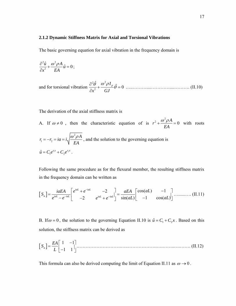
End Bearing Piles) ……………………………………………….............. 52
III.12 Effect of EP/ES on Normalized Imaginary Coefficients (c1) of Single Pile (ES=Constant=5E7, 2% Material Damping, No Threshold Distance,
End Bearing Piles) ……………………………………………….............. 53
III.13 Effect of Smax on Imaginary Stiffness Coefficients of a 6 by 6 Pile Group (EP=1000ES=5E10, 2% Material Damping, End Bearing Piles) ………… 53
III.14 Effect of Smax on Equivalent Dashpot Constant of a 6 by 6 Pile Group (EP=1000ES=5E10, 2% Material Damping, End Bearing Piles) ………… 54
III.15 Vertical Static Group Factors for Vertical Stiffness (EP/ES=1000, Floating Piles)...………………………………………….... 55
III.16 Vertical Static Group Factors for Vertical Stiffness (EP/ES=1000, End Bearing Piles)………………………………………..... 56
III.17 Effect of EP/ES on Vertical Group Factors (No Threshold Distance, Floating Piles) ………………………….……... 57
III.18 Effect of EP/ES on Vertical Group Factors (No Threshold Distance, End Bearing Piles) ……...……………………... 57

x
FIGURE Page
III.19 Effect of Number of Piles on Real Coefficients (EP=1000ES=5E10, 2% Material Damping, No Threshold Distance, Floating Piles) ………… 58
III.20 LSF of Equivalent Mass of Vertical Stiffness…………………………..... 59
III.21 Equivalent Mass with Number of Piles…………………..……………..... 60
III.22 Effect of Threshold Distance on Real Coefficients of 6 by 6 Pile Groups (EP=1000ES=5E10, 2% Material Damping, Floating Piles)…….………... 60
III.23 Effect of Number of Piles on Imaginary Coefficients (EP=1000ES=5E10, 2% Material Damping, No Threshold Distance, Floating Piles)..………... 60
III.24 Effect of EP/ES on Imaginary Coefficients of Single Piles (ES=Constant =5E10, 2% Material Damping, No Threshold Distance, Floating Piles).... 62
III.25 Static Group Reduction Factor for Rocking Stiffness (EP/ES=1000, Floating Piles) …………………..………………….……... 63
III.26 Static Group Reduction Factor for Rocking Stiffness (EP/ES=1000, End Bearing Piles)..……...…………….…………………... 64
III.27 Effect of EP/ES on Static Group Factor (No Threshold Distance, Floating Piles) …………….…………………... 65
III.28 Effect of EP/ES on Static Group Factor (No Threshold Distance, End Bearing Piles)…...…….…………………... 65
III.29 Effect of Number of Piles on Real Coefficients (EP=1000ES=5E10, 2% Material Damping, No Threshold Distance, Floating Piles).……….... 66
III.30 Least Square Fit of Equivalent Inertia of Rotation of Rocking Stiffness.... 67
III.31 Equivalent Inertia of Rotation with Number of Piles…………………...... 68
III.32 Effect of Limit Distance on Real Coefficients of 6 by 6 Pile Groups (EP=1000ES=5E10, 2% Material Damping, Floating Piles)...….……….... 69
III.33 Effect of Number of Piles on Imaginary Coefficients (EP=1000ES=5E10, 2% Material Damping, No Threshold Distance, Floating Piles)...….…..... 70

xi
FIGURE Page
III.34 Effect of EP/ES on Imaginary Coefficients of 2 by 2 Pile Groups (2% Material Damping, No Threshold Distance, Floating Piles).….…...... 70
IV.1 Piers and Pile Groups of Marga-Marga Bridge…………………….…...... 71
IV.2 A Pier and Its Pile Foundation………………..…………………….…...... 72
IV.3 Dimensions of Cap and Pile Spacing……………………………....…....... 73
IV.4 Real Part of Horizontal Stiffness in Y Direction…………………………. 77
IV.5 Imaginary Part of Horizontal Stiffness in Y Direction………...…………. 77
IV.6 Real Part of Horizontal Stiffness in X Direction…………………………. 78
IV.7 Imaginary Part of Horizontal Stiffness in X Direction………...…………. 78
IV.8 Real Part of Horizontal Stiffness of an Equivalent Surface Mat…………. 79
IV.9 Imaginary Part of Horizontal Stiffness of an Equivalent Surface Mat…… 79
IV.10 Real Part of Vertical Stiffness………………………………...………….. 80
IV.11 Imaginary Part of Vertical Stiffness…...……………………...………….. 82
IV.12 Real Part of Vertical Stiffness of an Equivalent Surface Mat……...…….. 82
IV.13 Imaginary Part of Vertical Stiffness of an Equivalent Surface Mat…..….. 83
IV.14 Real Part of Rocking Stiffness around X Axis………………………..….. 83
IV.15 Imaginary Part of Rocking Stiffness around X Axis………...………..….. 84
IV.16 Real Part of Rocking Stiffness around Y Axis………………………..….. 84
IV.17 Imaginary Part of Rocking Stiffness around Y Axis………...………..….. 85
IV.18 Real Part of Rocking Stiffness around X Axis of an Equivalent Surface Mat………..………………………………..….. 85
IV.19 Imaginary Part of Rocking Stiffness around X Axis of an Equivalent Surface Mat………..………………………………..….. 86

xii
FIGURE Page
IV.20 Real Part of Rocking Stiffness around Y Axis of an Equivalent Surface Mat………..………………………………..….. 86
IV.21 Imaginary Part of Rocking Stiffness around Y Axis of an Equivalent Surface Mat………..………………………………..….. 87
IV.22 Stiffness of Surface Mat of Pier #1 & Pier #7………….………………… 88
IV.23 New Real Part of Horizontal Stiffness in X Direction...…..……………... 91
IV.24 New Imaginary Part of Horizontal Stiffness in X Direction…..…..……... 91
IV.25 New Real Part of Horizontal Stiffness in Y Direction...…..……………... 92
IV.26 New Imaginary Part of Horizontal Stiffness in Y Direction…..…..……... 92
IV.27 New Real Part of Vertical Stiffness………………..………...………..….. 93
IV.28 New Imaginary Part of Vertical Stiffness………………………...…..…... 93
IV.29 New Real Part of Rocking Stiffness around X Axis……………...…..…... 94
IV.30 New Imaginary Part of Rocking Stiffness around X Axis…..………..….. 94
IV.31 New Real Part of Rocking Stiffness around Y Axis………...………..….. 95
IV.32 New Imaginary Part of Rocking Stiffness around Y Axis………..…..….. 95
IV.33 New Stiffness of Surface Mat under Pier #1 & Pier #7…….…………..… 96
V.1 Overview of Marga-Marga Bridge……………………………………….. 97
V.2 Cross Section of Deck……………………………………………………. 98
V.3 Transverse View of Pier and Its Dimensions…………………………….. 99
V.4 Cross Section of Pier……………………………………………….…….. 100
V.5 Rubber Pads on Top of Pier………………………………………..……... 101
V.6 Elements and Nodal Numbering of Marga-Marga Bridge (without Rubber Pads)…………………..………………………………... 103
xiii
FIGURE Page
V.7 Elements and Nodal Numbering of Marga-Marga Bridge (with Rubber Pads)…………………..…………………………….……... 104
V.8 Displacement in X Direction at Top of Pier 4 due to Unit Motion at Base of All Piers (without Rubber Pads)…….………………………… 106
V.9 Displacement in X Direction due to Unit Motion at Base of All Piers (with Rubber Pads, 66.0 10G = × Pa, Free Deck)………………………… 107
V.10 Displacement in X Direction due to Unit Motion at Base of Pier 4 (with Rubber Pads, 66.0 10G = × Pa, Free Deck)………………………… 108
V.11 Displacement in X Direction due to Unit Motion at Base of All Piers (with Rubber Pads, 61.8 10G = × Pa, Free Deck)…………………….…… 109
V.12 Displacement in X Direction due to Unit Motion at Base of All Piers (with Rubber Pads, 61.0 10G = × Pa, Free Deck)…………………….…… 109
V.13 Displacement in X Direction due to Unit Motion at Base of All Piers (with Rubber Pads, 66.0 10G = × Pa, Constrained Deck)………………… 111
V.14 Displacement in X Direction due to Unit Motion at Base of Pier 4 (with Rubber Pads, 66.0 10G = × Pa, Constrained Deck)………………… 111
V.15 Displacement in X Direction due to Unit Motion at Base of All Piers (with Rubber Pads, 61.8 10G = × Pa, Constrained Deck)…………….….. 112
V.16 Displacement in X Direction due to Unit Motion at Base of All Piers (with Rubber Pads, 61.0 10G = × Pa, Constrained Deck)…………….…... 112
V.17 Displacement in Y Direction at Top of Pier 4 due to Unit Motion at Base of All Piers (without Rubber Pads)…….………………………… 113
V.18 Displacement in Y Direction due to Unit Motion at Base of All Piers (with Rubber Pads, 66.0 10G = × Pa, Free Deck)………………………… 114
V.19 Displacement in Y Direction due to Unit Motion at Base of All Piers (with Rubber Pads, 61.8 10G = × Pa, Free Deck)…………………….…… 115

xiv
FIGURE Page
V.20 Displacement in Y Direction due to Unit Motion at Base of All Piers (with Rubber Pads, 61.0 10G = × Pa, Free Deck)…………………….…… 115
V.21 Displacement in Y Direction due to Unit Motion at Base of All Piers (with Rubber Pads, 66.0 10G = × Pa, Constrained Deck)………………… 116
V.22 Displacement in Y Direction due to Unit Motion at Base of All Piers (with Rubber Pads, 61.8 10G = × Pa, Constrained Deck)…………….….. 117
V.23 Displacement in Y Direction due to Unit Motion at Base of All Piers (with Rubber Pads, 61.0 10G = × Pa, Constrained Deck)…………….….. 117
V.24 Displacement in Z Direction at Top of Pier 4 due to Unit Motion at Base of All Piers (without Rubber Pads)…….………………………… 118
V.25 Displacement in Z Direction due to Unit Motion at Base of All Piers (with Rubber Pads, 91.8 10E = × Pa, Free Deck)…………………….…… 119
V.26 Displacement in Z Direction due to Unit Motion at Base of All Piers (with Rubber Pads, 91.8 10E = × Pa, Free Deck)…………………………. 120
VI.1 Displacement in X Direction at Top of Pier 4 due to Unit Motion at Base of All Foundations (without Rubber Pads)…….………………… 124
VI.2 Displacement in X Direction due to Unit Motion at Base of All Foundations (with Rubber Pads, 66.0 10G = × Pa, Free Deck)………………………… 126
VI.3 Displacement in X Direction due to Unit Motion at Base of Foundation under Pier 4 (with Rubber Pads, 66.0 10G = × Pa, Free Deck)..….………. 127
VI.4 Displacement in X Direction due to Unit Motion at Base of All Foundations (with Rubber Pads, 61.8 10G = × Pa, Free Deck)…………………….…… 127
VI.5 Displacement in X Direction due to Unit Motion at Base of All Foundations (with Rubber Pads, 61.0 10G = × Pa, Free Deck)…………………….…… 128
VI.6 Displacement in X Direction due to Unit Motion at Base of All Foundations (with Rubber Pads, 66.0 10G = × Pa, Constrained Deck)………………… 128

xv
FIGURE Page
VI.7 Displacement in X Direction due to Unit Motion at Base of the Foundation under Pier 4 (with Rubber Pads, 66.0 10G = × Pa, Constrained Deck)..….. 129
VI.8 Displacement in X Direction due to Unit Motion at Base of All Foundations (with Rubber Pads, 61.8 10G = × Pa, Constrained Deck)…………….…... 129
VI.9 Displacement in X Direction due to Unit Motion at Base of All Foundations (with Rubber Pads, 61.0 10G = × Pa, Constrained Deck)…………….…... 130
VI.10 Motion of the Base of Pier 4 When All Foundations Are Excited in the X Direction (Free Deck)…………………………………….…...… 130
VI.11 Motion of the Base of Pier 4 When All Foundations Are Excited in the X Direction (Constrained Deck)…………………………….…...… 131
VI.12 Displacement in Y Direction at Top of Pier 4 due to Unit Motion at Base of All Foundations (without Rubber Pads)…….………………… 132
VI.13 Displacement in Y Direction due to Unit Motion at Base of All Foundations (with Rubber Pads, 66.0 10G = × Pa, Free Deck)………………………… 133
VI.14 Displacement in Y Direction due to Unit Motion at Base of All Foundations (with Rubber Pads, 61.8 10G = × Pa, Free Deck)…………………….…… 134
VI.15 Displacement in Y Direction due to Unit Motion at Base of All Foundations (with Rubber Pads, 61.0 10G = × Pa, Free Deck)…………………….…… 134
VI.16 Displacement in Y Direction due to Unit Motion at Base of All Foundations (with Rubber Pads, 66.0 10G = × Pa, Constrained Deck)………………… 135
VI.17 Displacement in Y Direction due to Unit Motion at Base of All Foundations (with Rubber Pads, 61.8 10G = × Pa, Constrained Deck)…………….…... 135
VI.18 Displacement in Y Direction due to Unit Motion at Base of All Foundations (with Rubber Pads, 61.0 10G = × Pa, Constrained Deck)…………….…... 136
VI.19 Motion of the Base of Pier 4 When All Foundations Are Excited in the Y Direction (Free Deck)…………………………………….…...… 136

xvi
FIGURE Page
VI.20 Motion of the Base of Pier 4 When All Foundations Are Excited in the Y Direction (Constrained Deck)…………………………….…...… 137
VI.21 Displacement in Z Direction at Top of Pier 4 due to Unit Motion at Bottom of All Foundations (without Rubber Pads)…….……………… 138
VI.22 Displacement in Z Direction due to Unit Motion at Base of All Foundations (with Rubber Pads, 96.0 10E = × Pa, Free Deck)………………………… 138
VI.23 Displacement in Z Direction due to Unit Motion at Base of All Foundations (with Rubber Pads, 96.0 10E = × Pa, Free Deck)…………………….…... 139
VII.1 FFT of Recorded Longitudinal (X) Motion of Marga-Marga Bridge during the Earthquake of July 24, 2001…………………………………... 145
VII.2 FFT of Recorded Transverse (Y) Motion of Marga-Marga Bridge during the Earthquake of July 24, 2001…………………………………... 145
VII.3 FFT of Recorded Vertical (Z) Motion of Marga-Marga Bridge during the Earthquake of July 24, 2001………………………………….. 148
VII.4 One-dimensional Horizontal Soil Amplification of the Soil Deposit…….. 148
A.1 The 1st Mode Shape of the Bridge in Figure II.5…………………..……... 157
A.2 The 2nd Mode Shape of the Bridge in Figure II.5…...……………..……... 158
A.3 The 3rd Mode Shape of the Bridge in Figure II.5…………………..…….. 158
A.4 The 4th Mode Shape of the Bridge in Figure II.5…………………..….….. 159
A.5 The 5th Mode Shape of the Bridge in Figure II.5…………………..……... 159
A.6 The 6th Mode Shape of the Bridge in Figure II.5…………………..….….. 160
A.7 The 7th Mode Shape of the Bridge in Figure II.5…………………...…….. 160
A.8 The 8th Mode Shape of the Bridge in Figure II.5…………………..……... 161
A.9 The 9th Mode Shape of the Bridge in Figure II.5…………………..……... 161
A.10 The 10th Mode Shape of the Bridge in Figure II.5………………..………. 162

xvii
FIGURE Page
A.11 The 11th Mode Shape of the Bridge in Figure II.5………………..………. 162
A.12 The 12th Mode Shape of the Bridge in Figure II.5………………..………. 163
A.13 The 13th Mode Shape of the Bridge in Figure II.5………………..………. 163
A.14 The 14th Mode Shape of the Bridge in Figure II.5………………..………. 164
A.15 The 15th Mode Shape of the Bridge in Figure II.5………………..………. 164
A.16 The 16th Mode Shape of the Bridge in Figure II.5………………..………. 165
A.17 The 17th Mode Shape of the Bridge in Figure II.5………………..………. 165
A.18 The 18th Mode Shape of the Bridge in Figure II.5………………..………. 166
A.19 The 19th Mode Shape of the Bridge in Figure II.5………………..………. 166
A.20 The 20th Mode Shape of the Bridge in Figure II.5………………..………. 167
A.21 The 21st Mode Shape of the Bridge in Figure II.5………………..………. 167
A.22 The 22nd Mode Shape of the Bridge in Figure II.5…...…………..………. 168
A.23 The 23rd Mode Shape of the Bridge in Figure II.5………………..……… 168
A.24 The 24th Mode Shape of the Bridge in Figure II.5………………..………. 169
A.25 The 25th Mode Shape of the Bridge in Figure II.5………………..………. 169
A.26 The 26th Mode Shape of the Bridge in Figure II.5………………..………. 170
A.27 The 27th Mode Shape of the Bridge in Figure II.5………………..………. 170
A.28 The 28th Mode Shape of the Bridge in Figure II.5………………..………. 171
A.29 The 29th Mode Shape of the Bridge in Figure II.5………………..………. 171
A.30 The 30th Mode Shape of the Bridge in Figure II.5………………..………. 172

xviii
LIST OF TABLES
TABLE Page
II.1 Natural Frequencies for Different Values of Axial Load…………………. 20
II.2 Natural Frequencies and Mode Shapes Description of the Bridge in Figure II.5 (from ABAQUS) (Length of each segment is 0.05m).……………….. 33
II.3 Natural Frequencies and Mode Shapes Description of the Bridge in Figure II.5 (from ABAQUS) (Each member is considered as one segment, which is 10~14m-long)……………………………………………………. 34
II.4 Natural Frequencies and Mode Shapes Description of the Bridge in Figure II.5 (from ABAQUS) (Each member is considered as two segments, which is 5~7m-long)………………………………………………………. 35
II.5 Natural Frequencies and Mode Shapes Description of the Bridge in Figure II.5 (from ABAQUS) (Each member is about 3m-long)..……………….... 36
IV.1 Dimension of the Pier and Cap………………………………………...….. 73
IV.2 Length and Diameter of Piles……………………………………….…….. 74
IV.3 Soil Properties for Pier #2…….…………………………………….…….. 74
IV.4 Soil Properties for Pier #3 and #4…….…………………...………….…… 75
IV.5 Soil Properties for Pier #5…….…………………………………….…….. 75
IV.6 Soil Properties for Pier #6…….…………………………………….…….. 76
IV.7 Reduced Soil Properties for Pier #2…….……………………………..….. 89
IV.8 Reduced Soil Properties for Pier #3 and #4……………………………….. 89
IV.9 Reduced Soil Properties for Pier #5…….……………………………..….. 89
IV.10 Reduced Soil Properties for Pier #6…….…..………………………..……. 90
V.1 Natural Frequencies of Marga-Marga Bridge from Former Studies…….... 105
VI.1 Effect of SSI on Peaks of Transfer Function in Longitudinal Direction….. 125

xix
TABLE Page
VI.2 Effect of SSI on Peaks of Transfer Function in Transverse Direction….… 132
VI.3 Effect of SSI on Peaks of Transfer Function in Longitudinal Direction (with New Soil Properties)………………………………………………... 140
VI.4 Effect of SSI on Peaks of Transfer Function in Transverse Direction (with New Soil Properties)………………………………………………... 140

1
CHAPTER I
DESCRIPTION OF PROBLEM
1.1 Objective
The purpose of this work is to evaluate the effectiveness and efficiency of base isolation
on the seismic response of bridges and the potential importance of soil-structure
interaction effects. The dynamic stiffness of the complete system, including the
structure, the foundations and the isolation pads, is obtained in the frequency domain.
The transfer functions of the motions at some points on the bridge due to motions at the
base of all the piers or only one pier are calculated to examine the frequency response
characteristics of the system.
The objective of this research is to evaluate through some parametric studies the effects
of base isolation and soil structure interaction on the seismic response of bridges, with
application to a particular bridge, the Marga-Marga bridge, in Chile, for which data were
available, in order to use realistic parameters. This bridge uses hard rubber pads at the
abutments and on top of each pier for base isolation and has pile foundations for five of
its seven piers.
1.2 Base Isolation
Although I-Elastomeric bearings were first used in 1969 in Italy, base isolation
techniques were not widely used in civil structures to resist lateral forces before the
1990’s. Since the first design provisions appeared in the 1991 Uniform Building Code
(UBC), the use of base isolators as a part of a structure in addition to conventional
This dissertation follows the style and format of the Journal of Geotechnical and Environmental Engineering, ASCE.

2
materials (steel, concrete, etc.) has become more and more popular in severe seismic
hazard areas, and now base isolation plays an important part in the area of structural
control.
Extensive research has been done on the effect of base isolation on bridges since the
1990’s, when the technique started to be widely used to protect bridges from the effect
of seismic motions. Tan et al. (1993, 1996, 2000), Chaudhary et al. (1998, 2000, 2001a,
2001b, 2002a), Shinozuka et al. (2001) and Crouse and McGuire (2001) worked on the
system identification of base isolated bridges, in some cases considering the effect of
soil structure interaction. Park et al. (2002), Chaudhary et al. (2002b) and Su et al. (1989,
1990) used real earthquake records to investigate the behavior of base isolated bridges
and compared the performance of different kinds of base isolators.
Figure I.1 Normal Rubber Bearing (NRB)
(Made of Alternating Layers of Rubber and Steel)
The base isolators used in the Marga-Marga bridge are Normal Rubber Bearings (NRB).
As shown in Figure I.1, they are made of alternating layers of steel and rubber to achieve

3
a low horizontal stiffness with a high vertical stiffness, to provide a uniform transfer of
vertical load from the girder to the piers but to mitigate the horizontal load transfer from
the piers to the girder during the earthquake. The NRBs can extend the natural period of
the structure as well as absorb the earthquake energy though their hysteretic damping
(Skinner et al. 1993).
There have been many models proposed by researchers to study the behavior of the
isolated structure or of the bearings by themselves. Most of them have been nonlinear
models in the time domain to perform time history analysis. In some linear models, each
rubber layer of the bearing has been considered to be linear, homogeneous and isotropic
and treated as an equivalent column to calculate its stiffness matrix using beam theory
(Haringx, 1949). All rubber and steel layers were then combined to get the stiffness
matrix of the bearing pad and the matrix was then condensed to relate only end forces
and displacements (Chang, 2002). Seki et al. (1987), Takayama et al. (1990), Billings
(1993) and Matsuda (1999, 2001) developed two- or three-dimensional finite element
models of the NRBs to investigate the internal stress-strain relationship under large
deformations and gave some recommendations on the value of the hysteretic damping.
In this research, the whole rubber pad will be considered as an equivalent structural
member to evaluate its dynamic stiffness in the same way as for the structural members,
using Timoshenko beam theory.
1.3 Soil Structure Interaction (SSI)
The conventional design method of a building or a bridge assumes that the foundations
are fixed. The internal forces in the structural members, including the forces transferred
from the base columns or the piers to the foundation, are calculated, and the strength of
the foundation and settlements of the subsoil are then estimated. The problem is that the
settlement of the foundation will change the internal forces in the superstructure. The

4
stiffness of the foundation should be incorporated in the model of the structure to
perform a soil structure interaction analysis.
The effects of soil structure interaction (SSI) on the dynamic response of bridges have
been extensively studied. The superstructures were normally discretized into structural
members with concentrated or consistent mass matrices, while the foundations could be
modeled using different methods. The simplest model is to use Winkler’s assumption to
model the soils as springs to support spread footings or piles (Crouse et al. 1987; Casas,
1997; Mylonakis et al. 1997; McGuire et al. 1998; Hutchinson et al. 2004). With this
model the effect of inertia forces of the soil and the radiation damping were not
included. Other researchers (Levine and Scott, 1989; Spyrakos, 1990; Spyrakos and
Loannidis, 2003; Harada et al. 1994; Makins et al. 1994, 1996; Chaudhry and Prakash,
1998; Tongaokar and Jangid, 2003) modeled the soils or piles as a single degree freedom
with coefficients for the mass, spring and dashpot, as recommended by Wolf (1988).
Iwasaki et al. (1984) and Takemiya (1985) simplified the subsoil into a one-dimensional
soil column to calculate its dynamic stiffness. Finite element (Kuribaya and Iida, 1974;
Yamada and Kawano, 1979; Dendrou et al. 1984; Zheng and Takeda, 1995; Consolazio
et al. 2003) or Boundary element formulations (Betti, 1995; Guin and Banerjee, 1998)
were also widely used in the modeling of the soils and piles. Crouse and Price (1993),
Takemiya and Yamada (1981) and Saadeghvaziri et al. (2000) used analytical or semi-
analytical formulations similar to the one used in this research. Lee and Dasgupta (1984)
modeled the soil under the piers with nonlinear finite elements and the outer region with
an analytical frequency dependent stiffness. Other studies concentrated on the nonlinear
soil behavior (Hino and Tanabe, 1986; Zechlin and Chai, 1998; Carrubba et al. 2003).
In this work, the dynamic stiffness of pile groups is investigated using an Elasto-
dynamic solution with Poulos’ method (1971) in the frequency domain. The dynamic
stiffness of the surface foundations for the piers without pile foundations was calculated

5
using also an Elasto-dynamic solution. After combining the dynamic stiffness of the
structure and the foundation, the effect of soil structure interaction is evaluated.
1.4 Marga-Marga Bridge
The Marga-Marga bridge, shown schematically in Figure I.2, is an actual bridge in
Chile. The deck, which is 383 meters long, consists of 8 spans, all 50 meters long, except
for the first one (connecting the south abutment and pier 1), which is 33 meters long. On
top of each pier and of the two abutments are rubber pads (base isolators). The bridge
has seven piers (P1~P7), five of them (P2~P6) with pile foundations. Each of the pile
foundations consists of a 5 by 2 pile group (rows of 5 piles in the direction perpendicular
to the figure and 2 in the longitudinal direction of the bridge). Piers P1 and P7 have
surface mat foundations without any supporting piles. The bridge was instrumented after
construction and a number of earthquake records were obtained.
Pier
Girder
Rubber Pad(Base Isolator)
Pile Foundation
SurfaceFoundation
Figure I.2 The Marga-Marga Bridge
6
1.5 Previous Studies
Seismic analyses of the Marga-Marga bridge had been conducted by a number of
students at the University of Chile. M.E. Segovia developed in 1997 a model to calculate
the natural frequencies of the bridge with or without rubber pads; D. Romo (1999)
develop in 1999 a different model using finite elements (shell elements), studying the
effect of the boundary conditions at the two ends of the deck; Another finite element
model has implemented by V.M. Daza in 2003 including soil structure interaction
effects.
1.6 Outline of Research
The research conducted in this work consists of the following steps:
• Development of a computational model for a three-dimensional bridge structure
with distributed masses in the frequency domain. This model includes the piers,
girders and slab as well as the isolation pads. It will accept as input the dynamic
stiffness of the foundations, computed separately, as functions of frequency. The
model was implemented in a computer program and tested for accuracy;
• Determination of the dynamic stiffness terms for pile foundations. Some
preliminary studies were conducted to investigate the nature and importance of
group effects and the effect of limiting the interaction between piles when their
separation exceeds a given distance. The program developed to determine the
dynamic stiffness of pile groups was then used to compute the stiffness of the
pile foundations of the Marga-Marga bridge. A separate program was used to
compute the stiffness of the surface foundations of two piers;

7
• Parametric studies were conducted to assess the effectiveness of the base
isolation assuming first rigid foundations, without soil structure interaction
effects. The stiffness of the rubber pads was changed to study the effect of their
properties on the seismic response of the bridge, looking at the transfer functions
for the motions at various points due to unit motions at the base of the piers;
• The same type of studies were carried out including now soil structure interaction
effects to assess their potential importance;
1.7 Dissertation Outline
The formulation of the structural model in the frequency domain is presented in Chapter
II with some simple analyses to validate it. Chapter III discusses the dynamic stiffness of
pile groups. The results for the foundations of the Marga-Marga bridge are included in
Chapter IV. The effect of the stiffness of the rubber pads is investigated and reported in
Chapter V while Chapter VI presents the studies on soil structure interaction effects.
Conclusions and recommendations for further work are included in Chapter VII.

8
CHAPTER II
STRUCTURAL FORMULATION
2.1 Dynamic Stiffness Matrix of a Prismatic Member
The use of the dynamic stiffness matrices in the frequency domain for linear structural
members with distributed masses provides a more efficient and accurate procedure for
the dynamic analysis of frames than lumped or consistent mass matrices. The higher
accuracy provided is a major consideration in the interpretation of dynamic non-
destructive tests based on impact loads and wave propagation.
The dynamic stiffness matrix for linear structural members with distributed masses were
first used by Latona (1969) and extended by Papaleontiou (1992) later to validate the
accuracy of lumped and consistent mass matrices. Formulations for beam members and
shell elements were then obtained by Kolousěk (1973), Banerjee and William (1985,
1994a, 1994b), Doyle (1989a, 1989b), Gopalakrishnan and Doyle (1994) and Yu and
Roësset (2001). Chen and Sheu (1993, 1996), Yu (1995, 1996) and Yu and Roësset
(1998) used these formulations to carry out some studies on structural dynamics, soil
structure interaction and non-destructive testing. In this chapter, the derivation of the
dynamic stiffness matrix associated with the exact continuous solution is carried out
using the same approach followed to obtain the static stiffness matrix. The following
paragraphs give the main steps of this approach deriving the dynamic stiffness matrix of
a prismatic flexural member.
2.1.1 Dynamic Stiffness Matrix for Transverse Deflection
For the transverse behavior of a flexural member, the Timoshenko beam theory includes
the shear deformation and rotational inertia of the beam. The governing equations in the
frequency domain are

9
2
2
ˆ ˆ ˆ
ˆˆ
ˆˆ
ˆˆ ˆ( )
ˆˆ ˆ
M V Ix
Y Avx
M EIx
vV GAxvY V Nx
ω ρ ϕ
ω ρ
ϕ
κ ϕ
⎧∂+ = −⎪ ∂⎪
⎪∂= −⎪ ∂⎪
∂⎪ =⎨ ∂⎪∂⎪ = −⎪ ∂⎪∂⎪ = +
⎪ ∂⎩
.………………………..…………………………….……... (II.1)
in which
, ,E Gρ ………...………....density, Young’s modulus and shear modulus of the material;
, ,I Aκ ...effective shear area coefficient, moment of inertia and area of the cross section;
, , , ,M V Y vϕ ……………………….………………………….…..bending moment, shear
force, vertical force, bending rotation and transverse displacement of the cross section;
ˆ ˆ ˆ ˆ ˆ, , , ,M V Y ϕ ν ………………………..…... , , , ,M V Y vϕ in frequency domain, respectively;
N ………………………………………………...………………………….…axial force.
In this case, to obtain a linear ordinary differential equation with constant coefficients,
all the material properties and cross-section properties are assumed to be constant along
the beam. These properties include , , , , ,E G I Aρ κ and N .
After combining the above equations, we can get a governing equation with only one
unknown- v .
2 22 2ˆ ˆ ˆ1 1 " 1 0IVN A N IEI v EI N I v A v
GA GA GA GAω ρ ω ρω ρ ω ρ
κ κ κ κ⎡ ⎤ ⎛ ⎞⎛ ⎞ ⎛ ⎞+ + − + + + − =⎜ ⎟ ⎜ ⎟ ⎜ ⎟⎢ ⎥⎝ ⎠ ⎝ ⎠⎣ ⎦ ⎝ ⎠
……………...…………………………..…...…………………………….………… (II.2)

10
Solving this equation and finding v as a function of x andω , we can find M ,V , Y and
ϕ by substituting v back into Equation II.1.
Defining
2 2
2 22
21 1
11
A N IN N EIGA EIGA GA
A IN GAEIGA
ω ρ ω ρβκ
κ κ
ω ρ ω ρακ
κ
⎧= − +⎪ ⎛ ⎞ ⎛ ⎞⎜ ⎟ ⎜ ⎟⎪ + +⎜ ⎟ ⎜ ⎟⎪ ⎝ ⎠ ⎝ ⎠
⎨ ⎛ ⎞⎪ ⎜ ⎟= −⎜ ⎟⎜ ⎟⎪ ⎛ ⎞ ⎝ ⎠⎜ ⎟+⎪ ⎜ ⎟⎝ ⎠⎩
we get the characteristic equation 4 2 22 0r rβ α+ + = …………...….…….………. (II.3)
It is convenient to express the solution of Equation II.3 for three different cases.
A. Static case without axial force, 0ω = and 0N = ;
In this case, 22 0β α= = . The governing equation becomes ˆ 0IVEIv = . The solution
of this equation is 2 31 2 3 4v C C x C x C x= + + + . From Equation II.1, the expressions for the
bending moment, shear force, transverse force and bending rotation can be derived in
terms of the transverse displacement v . Since 0Nω = = , the expressions are
ˆ ˆ"ˆ ˆ ˆ
ˆ ˆ ˆ'
III
III
M EIv
Y V EIvEIv vGA
ϕκ
⎧=⎪
⎪= =⎨
⎪⎪ = +⎩
.…………………………………………………………….……. (II.4)
The end displacements u of this case can be expressed in terms of the constants iC .

11
[ ]
1
212 3
3
2 4
1 0 0 0ˆ ˆ(0) 60 1 0ˆ ˆ(0)
ˆˆ ˆ( ) 1
ˆˆ ( ) 60 1 2 3
A
A
B
B
Cv v EICGAu T CCv v L L L L
L EI CL LGA
ϕ ϕ κ
ϕϕκ
⎡ ⎤⎢ ⎥ ⎧ ⎫⎧ ⎫ ⎧ ⎫⎢ ⎥ ⎪ ⎪⎪ ⎪ ⎪ ⎪⎪ ⎪ ⎪ ⎪ ⎪ ⎪⎢ ⎥= = = =⎨ ⎬ ⎨ ⎬ ⎨ ⎬⎢ ⎥⎪ ⎪ ⎪ ⎪ ⎪ ⎪⎢ ⎥⎪ ⎪ ⎪ ⎪ ⎪ ⎪⎩ ⎭ ⎢ ⎥⎩ ⎭ ⎩ ⎭+⎢ ⎥⎣ ⎦
.
The end forces F can also expressed in terms of the constants iC .
[ ]
1
22
3
4
ˆ ˆ(0) 0 0 0 6ˆ ˆ (0) 0 0 2 0ˆˆ ˆ 0 0 0 6( )
0 0 2 6ˆˆ ( )
A
A
B
B
Y Y CCM M
F T CCY Y L
L CM LM
⎧ ⎫ ⎧ ⎫− ⎧ ⎫⎡ ⎤⎪ ⎪ ⎪ ⎪ ⎪ ⎪⎢ ⎥− −⎪ ⎪ ⎪ ⎪ ⎪ ⎪⎢ ⎥= = = =⎨ ⎬ ⎨ ⎬ ⎨ ⎬−⎢ ⎥⎪ ⎪ ⎪ ⎪ ⎪ ⎪⎢ ⎥⎪ ⎪ ⎪ ⎪ ⎪ ⎪⎣ ⎦ ⎩ ⎭⎩ ⎭⎩ ⎭
.
The computation of the stiffness matrix fS⎡ ⎤⎣ ⎦ can be carried out numerically as
[ ] [ ][ ] 12 2 1
ˆ ˆ ˆfF T C T T u S u− ⎡ ⎤= = = ⎣ ⎦
[ ][ ] 12 1fS T T −⎡ ⎤ =⎣ ⎦
The result can be written in explicit form as
3 2 3 2
2 2
3 2 3 2
2 2
12 6 12 6
6 2(2 ) 6 2(1 )
12 6 12 61 2
6 2(1 ) 6 2(2 )
f
L L L L
EI L L L LS
L L L L
L L L L
η η
η
η η
⎡ ⎤−⎢ ⎥⎢ ⎥
+ −⎢ ⎥−⎢ ⎥⎡ ⎤ = ⎢ ⎥⎣ ⎦ + ⎢ ⎥− − −
⎢ ⎥⎢ ⎥− +
−⎢ ⎥⎢ ⎥⎣ ⎦
...…..……….……..……….……. (II.5)
in which 2
6EIGAL
ηκ
= .

12
B. For static case with axial force, 0ω = and 0N ≠ ;
In this case, 2 0α = , but 2 01
NNEIGA
β
κ
−= ≠
⎛ ⎞+⎜ ⎟⎝ ⎠
. The governing equation becomes
ˆ ˆ1 " 0IVNEI v NvGAκ
⎛ ⎞+ − =⎜ ⎟⎝ ⎠
.
The solution to this equation is 1 21 2 3 4ˆ r x r xv C C x C e C e= + + + , in which 1 2 2r r β= − = − .
The expressions of bending moment, shear force, transverse force and bending rotation
in the frequency domain are
ˆ ˆ1 "
ˆ ˆ1
ˆ ˆ ˆ ˆ ˆ' ' 1
ˆ ˆ ˆ' 1
III
III
III
NM EI vGANV EI vGA
NY V Nv Nv EI vGA
EI Nv vGA GA
κ
κ
κ
ϕκ κ
⎧ ⎛ ⎞= +⎜ ⎟⎪ ⎝ ⎠⎪⎪ ⎛ ⎞= − +⎜ ⎟⎪⎪ ⎝ ⎠⎨
⎛ ⎞⎪ = + = − +⎜ ⎟⎪ ⎝ ⎠⎪
⎛ ⎞⎪ = + +⎜ ⎟⎪ ⎝ ⎠⎩
……………….....……...…………….……. (II.6)
The end displacements u and end forces F can be expressed in terms of the
constants iC .
[ ] 1 2
1 2
11 2
21
3
41 2
1 0 1 1ˆ ˆ(0)
0 1 1 1ˆ ˆ(0)ˆ
ˆ ˆ( ) 1ˆˆ ( )
0 1 1 1
A
Ar L r L
B
r L r LB
Cv v N Nr rCGA GA
u T CCv v L L e e
L CN Nr e r eGA GA
ϕ ϕ κ κ
ϕϕκ κ
⎡ ⎤⎢ ⎥ ⎧ ⎫⎧ ⎫ ⎧ ⎫ ⎛ ⎞ ⎛ ⎞⎢ ⎥+ + ⎪ ⎪⎪ ⎪ ⎜ ⎟ ⎜ ⎟⎪ ⎪ ⎢ ⎥⎪ ⎪ ⎪ ⎪ ⎝ ⎠ ⎝ ⎠ ⎪ ⎪= = = =⎨ ⎬ ⎨ ⎬ ⎨ ⎬⎢ ⎥
⎪ ⎪ ⎪ ⎪ ⎪ ⎪⎢ ⎥⎪ ⎪ ⎪ ⎪ ⎪ ⎪⎢ ⎥⎛ ⎞ ⎛ ⎞⎩ ⎭⎩ ⎭ ⎩ ⎭+ +⎢ ⎥⎜ ⎟ ⎜ ⎟
⎝ ⎠ ⎝ ⎠⎣ ⎦
13
1 2
12 21 2
2
3
2 2 41 2
0 0 0ˆ ˆ(0)
0 0 1 1ˆ ˆ (0)ˆˆ ˆ 0 0 0( )
ˆˆ ( ) 0 0 1 1
A
A
B
r L r LB
NY Y CN NEI r EI r
CM M GA GAF
CNY Y LCN NM LM EI r e EI r e
GA GAT
κ κ
κ κ
−⎡ ⎤⎢ ⎥⎧ ⎫ ⎧ ⎫− ⎧ ⎫⎛ ⎞ ⎛ ⎞⎢ ⎥⎪ ⎪ ⎪ ⎪ − + − + ⎪ ⎪⎜ ⎟ ⎜ ⎟− ⎢ ⎥⎪ ⎪ ⎪ ⎪ ⎝ ⎠ ⎝ ⎠ ⎪ ⎪= = =⎨ ⎬ ⎨ ⎬ ⎨ ⎬⎢ ⎥
⎪ ⎪ ⎪ ⎪ ⎪ ⎪⎢ ⎥⎪ ⎪ ⎪ ⎪ ⎪ ⎪⎢ ⎥⎛ ⎞ ⎛ ⎞ ⎩ ⎭⎩ ⎭⎩ ⎭ + +⎢ ⎥⎜ ⎟ ⎜ ⎟
⎝ ⎠ ⎝ ⎠⎣ ⎦= [ ] 2 C
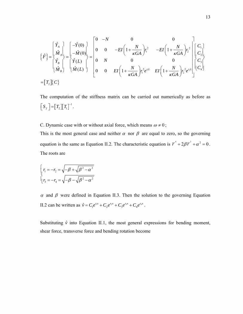
The computation of the stiffness matrix can be carried out numerically as before as
[ ][ ] 12 1fS T T −⎡ ⎤ =⎣ ⎦ .
C. Dynamic case with or without axial force, which means 0ω ≠ ;
This is the most general case and neither α nor β are equal to zero, so the governing
equation is the same as Equation II.2. The characteristic equation is 4 2 22 0r rβ α+ + = .
The roots are
2 21 2
2 23 4
r r
r r
β β α
β β α
⎧ = − = − + −⎪⎨⎪ = − = − − −⎩
α and β were defined in Equation II.3. Then the solution to the governing Equation
II.2 can be written as 31 2 41 2 3 4ˆ r xr x r x r xv C e C e C e C e= + + + .
Substituting v into Equation II.1, the most general expressions for bending moment,
shear force, transverse force and bending rotation become

14
2
2
2 2
2
2
ˆ ˆ ˆ1 "
1ˆ ˆ ˆ1 1 '
ˆ ˆ ˆ '
1ˆ ˆ ˆ' 1
III
III
N AM EI v vGA GA
GA N AV EI v GA GA EI vGA I GA GA I GA
Y V Nv
A NGA EI v EI vGA I GA GA
ω ρκ κ
κ ω ρκ κκ ω ρ κ κ ω ρ κ
ω ρϕ κκ ω ρ κ κ
⎧ ⎡ ⎤⎛ ⎞= + +⎪ ⎜ ⎟⎢ ⎥⎝ ⎠⎣ ⎦⎪⎪ ⎡ ⎤⎛ ⎞⎛ ⎞⎪ = − + − + −⎢ ⎥⎜ ⎟ ⎜ ⎟⎪ − −⎝ ⎠ ⎝ ⎠⎣ ⎦⎨⎪ = +⎪⎪ ⎡ ⎤⎛ ⎞ ⎛ ⎞⎪ = + + +⎢ ⎥⎜ ⎟⎜ ⎟− ⎝ ⎠⎪ ⎝ ⎠⎣ ⎦⎩
.... (II.7)
Equation II.7 can be simplified using the characteristic equation 4 2 22 0r rβ α+ + = as
242
1
24
1
24
1
24
1
ˆ 1
ˆ ˆ '
ˆ
ˆ 1
i
i
i
i
r xi i
i
r xi i
i i
r xi
i i
r xi i
i i
N AM EI r C eGA GA
AV Y Nv Nr C er
AY C er
N Ar C eGA GAr
ω ρκ κ
ω ρ
ω ρ
ω ρϕκ κ
=
=
=
=
⎧ ⎡ ⎤⎛ ⎞= + +⎪ ⎜ ⎟⎢ ⎥⎝ ⎠⎣ ⎦⎪⎪ ⎛ ⎞⎪ = − = − +⎜ ⎟⎪ ⎝ ⎠⎨⎪ = −⎪⎪⎪ ⎡ ⎤⎛ ⎞= + +⎪ ⎢ ⎥⎜ ⎟
⎝ ⎠⎣ ⎦⎩
∑
∑
∑
∑
.
The end displacements u and end forces F can also be derived in the same way as
before.
[ ] 31 2 4
31 2 4
1
21 2 3 41
3
1 2 3 4 4
ˆ ˆ 1 1 1 1(0)ˆ ˆ(0)
ˆˆ ˆ( )
ˆˆ ( )
A
Ar Lr L r L r L
Br Lr L r L r L
B
Cv vCR R R R
u T Ce e e e Cv v L
R e R e R e R eL C
ϕ ϕ
ϕϕ
⎧ ⎫⎧ ⎫ ⎧ ⎫ ⎡ ⎤⎪ ⎪⎪ ⎪ ⎢ ⎥⎪ ⎪⎪ ⎪ ⎪ ⎪ ⎪ ⎪⎢ ⎥= = = =⎨ ⎬ ⎨ ⎬ ⎨ ⎬⎢ ⎥⎪ ⎪ ⎪ ⎪ ⎪ ⎪⎢ ⎥⎪ ⎪ ⎪ ⎪ ⎪ ⎪⎩ ⎭ ⎣ ⎦⎩ ⎭ ⎩ ⎭

15
31 2 4
31 2
2 2 2 2
1 2 3 4
1 1 2 2 3 3 4 42 2 2 2
1 2 3 4
1 1 2 2 3 3 4 4
ˆ ˆ(0)ˆ ˆ (0)ˆˆ ˆ( )
ˆˆ ( )
A
A
r Lr L r L r LB
Br Lr L r L
A A A AY Y r r r rM EIR r EIR r EIR r EIR rM
FA A A AY Y L e e e e
r r r rM LMEIR re EIR r e EIR r e EIR r e
ω ρ ω ρ ω ρ ω ρ
ω ρ ω ρ ω ρ ω ρ
⎧ ⎫ ⎧ ⎫−⎪ ⎪ ⎪ ⎪
− − − −−⎪ ⎪ ⎪ ⎪= = =⎨ ⎬ ⎨ ⎬⎪ ⎪ ⎪ ⎪ − − − −⎪ ⎪ ⎪ ⎪
⎩ ⎭⎩ ⎭
[ ]
4
1
2
3
4
2
r L
CCCC
T C
⎡ ⎤⎢ ⎥ ⎧ ⎫⎢ ⎥ ⎪ ⎪⎢ ⎥ ⎪ ⎪⎢ ⎥ ⎨ ⎬⎢ ⎥ ⎪ ⎪⎢ ⎥ ⎪ ⎪⎩ ⎭⎢ ⎥⎢ ⎥⎣ ⎦
=
in which ( )2
1 , 1, 2,3,4i ii
N AR r iGA GAr
ω ρκ κ
⎛ ⎞⎜ ⎟= + + =⎜ ⎟⎝ ⎠
. The computation of the stiffness
matrix can be carried out numerically again as [ ][ ] 12 1fS T T −⎡ ⎤ =⎣ ⎦ .
The resulting stiffness matrices for case A and B can also be derived from the limit of
fS⎡ ⎤⎣ ⎦ for this case as 00N
ω →⎧⎨ →⎩
and 0ω → , respectively.
In Equation II.7, if 2GA Iκ ω ρ= , the denominators of V and ϕ will become zero. So for
this special case, the governing equation becomes
( )ˆ ˆ1 ' 0IIINEI v EA GA vGA
κκ
⎛ ⎞+ + + =⎜ ⎟⎝ ⎠
………………...……...………..…..…… (II.8)
The corresponding characteristic equation is ( )31 0NEI r EA GA rGA
κκ
⎛ ⎞+ + + =⎜ ⎟⎝ ⎠
with roots
1
2 3
0
1
r
EA GAr rNEIGA
κ
κ
=⎧⎪⎪ +
= − =⎨⎛ ⎞⎪ +⎜ ⎟⎪ ⎝ ⎠⎩
. The solution to the governing Equation II.8 can
be written as 321 2 3ˆ r xr xv C C e C e= + + .

16
Substituting v into Equation II.1, the expressions for bending moment, shear force,
transverse force and bending rotation can be written as
( )
2 232
12
2 2 23
1 42
22
1
ˆ ˆ ˆ1 " 1
ˆ ˆ ˆ1 ' 1
ˆ ˆ ˆ '
i
i
r xi
i
r xi
i i
ii
N A N AM EI v v EIC EI r eGA GA GA GA
N A A N Av v dx C x r e CGA GA GA GA GAr
AV GA v AC x Nrr
ω ρ ω ρκ κ κ κ
ω ρ ω ρ ω ρϕκ κ κ κ κ
ω ρκ ϕ ω ρ
=
=
⎡ ⎤ ⎡ ⎤⎛ ⎞ ⎛ ⎞= + + = + + +⎜ ⎟ ⎜ ⎟⎢ ⎥ ⎢ ⎥⎝ ⎠ ⎝ ⎠⎣ ⎦ ⎣ ⎦⎡ ⎤⎛ ⎞ ⎛ ⎞= + + = + + + +⎜ ⎟ ⎜ ⎟⎢ ⎥⎝ ⎠ ⎝ ⎠⎣ ⎦
= − − = − − +
∑
∑∫3
42
232
1 42
ˆ ˆ ˆ '
i
i
r x
i
r x
i i
e GAC
AY V Nv AC x e GACr
κ
ω ρω ρ κ
=
=
⎧⎪⎪⎪⎪⎪⎨
⎛ ⎞⎪ −⎜ ⎟⎪ ⎝ ⎠⎪⎪
= + = − − −⎪⎩
∑
∑
... (II.9)
The end displacements and end forces are
[ ] 32
32
1
22 31
3
2 3 4
ˆ ˆ 1 1 1 0(0)ˆ ˆ 0 1(0)
ˆˆ ˆ 1 0( )
ˆˆ 1( )
A
Ar Lr L
Br Lr L
B
Cv vCR R
u T Ce e Cv v L
L R e R eL C
ϕ ϕ
ϕϕ
⎧ ⎫⎧ ⎫ ⎧ ⎫ ⎡ ⎤⎪ ⎪⎪ ⎪ ⎢ ⎥⎪ ⎪⎪ ⎪ ⎪ ⎪ ⎪ ⎪⎢ ⎥= = = =⎨ ⎬ ⎨ ⎬ ⎨ ⎬⎢ ⎥⎪ ⎪ ⎪ ⎪ ⎪ ⎪⎢ ⎥⎪ ⎪ ⎪ ⎪ ⎪ ⎪⎩ ⎭ ⎣ ⎦⎩ ⎭ ⎩ ⎭
[ ]32
32
2 2
12 3
22 2 3 322 2
3
2 3 4
2 2 3 3
0ˆ ˆ(0)ˆ ˆ 0(0)ˆˆ ˆ( )
ˆˆ ( )0
A
A
r Lr LB
Br Lr L
A A GAY Y Cr rCM EI EIR r EIR rM
F TCA AY Y L GAL e e GA
r r CM LMEI EIR r e EIR r e
ω ρ ω ρ κ
ω ρ ω ρκ κ
⎡ ⎤⎢ ⎥⎧ ⎫ ⎧ ⎫− ⎧ ⎫⎢ ⎥⎪ ⎪ ⎪ ⎪ ⎪ ⎪⎢ ⎥− − −−⎪ ⎪ ⎪ ⎪ ⎪ ⎪= = = =⎨ ⎬ ⎨ ⎬ ⎢ ⎥ ⎨ ⎬
⎪ ⎪ ⎪ ⎪ ⎢ ⎥ ⎪ ⎪− − − −⎪ ⎪ ⎪ ⎪ ⎢ ⎥ ⎪ ⎪⎩ ⎭⎩ ⎭⎩ ⎭ ⎢ ⎥
⎢ ⎥⎣ ⎦
C
in which ( )2
1 , 1, 2,3,4i ii
N AR r iGA GAr
ω ρκ κ
⎛ ⎞⎜ ⎟= + + =⎜ ⎟⎝ ⎠
. The computation of the stiffness
matrix can be carried out numerically as [ ][ ] 12 1fS T T −⎡ ⎤ =⎣ ⎦ .
17
2.1.2 Dynamic Stiffness Matrix for Axial and Torsional Vibrations
The basic governing equation for axial vibration in the frequency domain is
2 2
2
ˆ ˆ 0u A ux EA
ω ρ∂+ =
∂;
and for torsional vibration 22
2
ˆ ˆ 0pIx GJ
ω ρθ θ∂+ =
∂ …..………....…………....………. (II.10)
The derivation of the axial stiffness matrix is
A. If 0ω ≠ , then the characteristic equation of is 2
2 0ArEA
ω ρ+ = with roots
2
1 2Ar r ia i
EAω ρ
= − = = , and the solution to the governing equation is
1 21 2ˆ r x r xu C e C e= + .
Following the same procedure as for the flexural member, the resulting stiffness matrix
in the frequency domain can be written as
[ ] cos( ) 121 cos( )sin( )2
iaL iaL
a iaL iaL iaL iaL
aLe eiaEA aEASaLe e aLe e
−
− −
−⎡ ⎤+ − ⎡ ⎤= =⎢ ⎥ ⎢ ⎥−− − + ⎣ ⎦⎣ ⎦
…......…. (II.11)
B. If 0ω = , the solution to the governing Equation II.10 is 1 2u C C x= + . Based on this
solution, the stiffness matrix can be derived as
[ ] 1 11 1a
EASL
−⎡ ⎤= ⎢ ⎥−⎣ ⎦
.……………………….…..……………….….……..….……. (II.12)
This formula can also be derived computing the limit of Equation II.11 as 0ω → .

18
[ ]
[ ] ( )( ) [ ]
0 0
0
0 0
00 0
cos( ) 1lim
1 cos( )sin( )
cos( ) 1lim
1 cos( )sin( )
lim cos( ) lim 1lim
sin( ) lim 1 lim cos( )
1 11 1
a
a
a a
aa a
aLaEASaLaL
aLaEAaLaL
aLaEAaL aL
EAL
ω ω= →
→
→ →
→→ →
⎛ − ⎞⎡ ⎤= ⎜ ⎟⎢ ⎥−⎣ ⎦⎝ ⎠
⎛ − ⎞⎡ ⎤= ⎜ ⎟⎢ ⎥−⎣ ⎦⎝ ⎠
⎡ ⎤−⎛ ⎞ ⎢ ⎥= ⎜ ⎟ −⎢ ⎥⎝ ⎠ ⎣ ⎦−⎡ ⎤
= ⎢ ⎥−⎣ ⎦
The torsional stiffness matrix can be obtained just changing EA and Aρ into GJ and
pIρ in [ ]aS , respectively.
After deriving the fS⎡ ⎤⎣ ⎦ , [ ]aS and [ ]TS matrices, they can be assembled to get the
general stiffness matrix [ ]S in three dimensions.
2.2 Verification of the Program Spfram.for
Using the formulation described above a FORTRAN program was implemented to
perform dynamic analysis of three-dimensional frames. The program Spfram.for consists
of two parts:
• subroutines to compute the stiffness matrix of a single member;
• subroutines to assemble the global stiffness matrix and solve the system of linear
equations.
To test the program, a case was run to find the natural frequencies and buckling load of a
beam comparing the results with the analytical solution.
For a three-dimensional beam pinned at two ends in one direction, as shown in Figure
II.1, the natural frequencies and buckling load can be easily found analytically.

19
Figure II.1 A Beam Pinned at Two Ends
At end A, the rotation around the Z axis is free; at end B, the rotation around the Z axis
and the displacement along the X axis are free. All other end displacements are
constrained. The governing equation of this beam is also Equation II.2. The mode shapes
(Eigen-functions) of this pinned beam are
( )ˆ sin , 1,2...........nn xv C n
Lπ
= = ,
because they satisfy both the boundary conditionsˆ ˆ( 0) ( ) 0
ˆ ˆ( 0) ( ) 0M x M x Lv x v x L
⎧ = = = =⎨
= = = =⎩ and
governing Equation II.2.
Substituting the first mode shape into Equation II.2 to find the first natural frequency and
first buckling load, the resulting formula in implicit form is obtained
4 2 2 22 2
4 21 1 1 0N A N IEI EI N I AGA L GA GA L GA
π ω ρ π ω ρω ρ ω ρκ κ κ κ
⎡ ⎤ ⎛ ⎞⎛ ⎞ ⎛ ⎞+ − − + + + − =⎜ ⎟⎜ ⎟ ⎜ ⎟⎢ ⎥⎝ ⎠ ⎝ ⎠⎣ ⎦ ⎝ ⎠.. (II.13)
If we know the axial force N , we can compute the corresponding natural frequency ω
from this equation. For a given frequency ω one can compute on the other hand the
buckling load N .

20
For a rectangular-cross-section with
10 3
2 4
1 10 , 0.25 , 1000 /59 , 2.25 , 10 ,6z
E Pa kg m
A m I m L m
ν ρ
κ
⎧ = × = =⎪⎨
= = = =⎪⎩
,
the natural frequencies corresponding to different values of the axial load are
summarized in Table II.1.
Table II. 1 Natural Frequencies for Different Values of Axial Load
Axial Load (N)
Natural Frequency from Analytical Solution
(HZ)
Natural Frequency from Program Spfram.for
(HZ) 1000000000 28.8830 28.883 500000000 26.4246 26.425
0 23.7127 23.713 -500000000 20.6475 20.647 -1000000000 17.0395 17.039 -1500000000 12.4244 12.424 -2000000000 4.2881 4.288 -2067612136
(Buckling Load) 0 0.000
With program Spfram.for, a unit bending moment was applied at end B as shown in
Figure II.1. The output provided the end rotations as a function of frequency for a given
axial load. When the rotation at end B became infinite, the frequency was the natural
frequency. The results from the program are also tabulated in Table II.1.
The results indicate that the program is working correctly.

21
2.3 Program Bridge.for
2.3.1 Introduction to the Program
The ultimate goal of this work was to study the seismic behavior of the Marga-Marga
bridge (Figure II.2), assessing the effect of the isolation rubber pads between the girders
and piers (Figure II.3) and the potential importance of soil structure interaction.
A second program Bridge.for was implemented to analyze a bridge under seismic
loading in the frequency domain using the direct stiffness method. The program mainly
consists of three parts:
• a main program to perform the nodal and element generation;
• subroutines to compute the stiffness matrix of the members;
• subroutines to assemble the global stiffness matrix and solve the linear equations.
The last two parts are identical to those of the Spfram.for program.
Figure II.2 Overview of the Marga-Marga Bridge in Chile

22
There are in general three kinds of structural members: deck, piers and rubber pads
(Figures II.4 and II.5). To assess the effect of isolation pads the program allows
including or omitting the rubber pads in order to compare the corresponding response.
Figure II.3 Cross Section of the Bridge
If there are n piers, the deck will consist of 1n + members, as shown in Figure II.2. If
there are rubber pads, rubber pads are on the top of each pier. All the rubber pads on the
top of one pier are regarded as one member in the program. In the program, each pier is
divided into 3 members according to changes of the cross section to accommodate a
situation as shown in Figure II.3, because the stiffness matrix derived before is only
valid for prismatic members with constant cross section.
Figures II.4 and II.5 show the nodal and element numbers of the bridge for the cases
with and without rubber pads. In the two figures, dashed lines represent the deck
members, while continuous lines and solid lines represent the pier members and rubber
pads, if they exist, respectively.

23
5
6
1
17
7
8
9
10
13
14
2
11
12
3
15
16
4
18
Figure II.4 Nodal and Element Number of a Bridge with Rubber Pads
5
6
1
7
12
8
9
11
10
2
13
3 4
Figure II.5 Nodal and Element Number of a Bridge without Rubber Pads
2.3.2 Stiffness Matrix Transformation
The deck members consist of the deck itself and the steel girders. They are modeled as
an equivalent member. The centroidal axis of these equivalent members will be at some
vertical distance from the top of the piers or the rubber pads. To account for this
eccentricity rigid links are assumed between the centroidal axis of the equivalent deck
member and the top surface of the rubber pads (points A and 'A in Figure II.6).

24
Figure II.6 Forces and Displacements Transformation of Deck Members
One way to incorporate the rigid links is to transform the stiffness matrix of the deck
members. If we assume that the cross section cannot deform out of the plane, the
relationship between the displacements at A and 'A is
( )( )
( ) ( )( ) ( )( ) ( )
' 1 '
' 1 '
'
'
'
'
A A y A
A A x A
A A
x xA A
y yA A
z zA A
u u D
v v D
w w
θ
θ
θ θ
θ θ
θ θ
⎧ = +⎪⎪ = −⎪
=⎪⎨ =⎪⎪ =⎪⎪ =⎩
.
The relationship in matrix form is

25
( )( )( )
( )( )( )
[ ]
'1
'1
'
'
'
'
'
1 0 0 0 00 1 0 0 00 0 1 0 0 00 0 0 1 0 00 0 0 0 1 00 0 0 0 0 1
A A
A A
A A
x xA A
y yA A
z zA A
A U A
u uDv vDw w
U L U
θ θ
θ θ
θ θ
⎧ ⎫ ⎧ ⎫⎡ ⎤⎪ ⎪ ⎪ ⎪⎢ ⎥⎪ ⎪ ⎪ ⎪−⎢ ⎥⎪ ⎪ ⎪ ⎪⎢ ⎥⎪ ⎪ ⎪ ⎪=⎨ ⎬ ⎨ ⎬⎢ ⎥⎪ ⎪ ⎪ ⎪⎢ ⎥⎪ ⎪ ⎪ ⎪⎢ ⎥⎪ ⎪ ⎪ ⎪⎢ ⎥
⎢ ⎥⎣ ⎦⎪ ⎪ ⎪ ⎪⎩ ⎭ ⎩ ⎭=
.………….…....………..………….. (II.14)
where [ ]UL is the transformation matrix.
The transformation matrix for forces is derived in the same way as that of for
displacements.
( ) ( )( ) ( )( ) ( )( ) ( ) ( )( ) ( ) ( )( ) ( )
'
'
'
1' '
1 ''
'
x xA A
y yA A
z zA A
x x yA A A
y y x AA A
z zA A
F F
F F
F F
M M D F
M M D F
M M
⎧ =⎪
=⎪⎪
=⎪⎪⎨
= +⎪⎪
= −⎪⎪
=⎪⎩
( )( )( )( )( )( )
( )( )( )( )( )( )
'
'
'
1 '
1'
'
1 0 0 0 0 00 1 0 0 0 00 0 1 0 0 00 0 1 0 0
0 0 0 1 00 0 0 0 0 1
x xA A
y yA A
z zA A
x xA A
y yA A
z zA A
F F
F F
F F
DM MDM M
M M
⎧ ⎫ ⎧ ⎫⎡ ⎤⎪ ⎪ ⎪ ⎪⎢ ⎥⎪ ⎪ ⎪ ⎪⎢ ⎥⎪ ⎪ ⎪ ⎪⎢ ⎥⎪ ⎪ ⎪ ⎪⎪ ⎪ ⎪ ⎪=⎨ ⎬ ⎨ ⎬⎢ ⎥
⎪ ⎪ ⎪ ⎪⎢ ⎥⎪ ⎪ ⎪ ⎪⎢ ⎥−⎪ ⎪ ⎪ ⎪⎢ ⎥
⎢ ⎥⎣ ⎦⎪ ⎪ ⎪ ⎪⎪ ⎪ ⎪ ⎪⎩ ⎭ ⎩ ⎭
.………….……..…..…..……….. (II.15)
[ ] 'A F AF L F= or [ ] [ ] 1'
TA F A U AF L F L F−= = because [ ] [ ]1 T
F UL L− = .

26
We can then derive the transformed stiffness matrix for a span member as below in
Figure II.7.
Figure II.7 Stiffness Matrix Transformation of Deck Members
( ) ( ) ( ) ( ) ( ) ( )
( ) ( ) ( ) ( ) ( ) ( ) ( ) ( ) ( ) ( ) ( ) ( )
( ) ( ) ( ) ( ) ( ) ( )
( ) ( ) ( ) ( ) ( )' ' ' ' ' ' ' '' ' ' '' '
' ' ''
, , , , , , , , , , , ,
, , , , , , , , , , ,
,
' , , , , , , , , , , , ,
' , , , ,
T TA A A x y z B B B x y z A BA A B BA B
T
x y z x y z x y z x y zA A A A B B B BA A B B
TA B
T TA A A x y z B B B x y z A BA A B BA B
x y z x yA A AA A
U u v w u v w U U
F F F F M M M F F F M M M
F F
U u v w u v w U U
F F F F M M
θ θ θ θ θ θ
θ θ θ θ θ θ
= =
=
=
= =
= ( ) ( ) ( ) ( ) ( ) ( ) ( )
' ' ' ' '' ' '
' '
, , , , , , ,
,
T
z x y z x y zA B B B BB B
TA B
M F F F M M M
F F=
[ ]
[ ]
[ ][ ]
[ ]
[ ][ ]
[ ] [ ][ ]
[ ][ ]
[ ] [ ][ ]
[ ]
1 1
1 1
1
1
0 0'
0 0
0 00 0' '
0 00 0
' '
F FA A
F FB B
TF UU UA AA A
TU UB BF UB B
L LF F S U
L L
L LL LS U S U
L LL L
S U
− −
− −
−
−
⎡ ⎤ ⎡ ⎤⎢ ⎥ ⎢ ⎥= =⎢ ⎥ ⎢ ⎥⎣ ⎦ ⎣ ⎦
⎡ ⎤ ⎡ ⎤⎡ ⎤ ⎡ ⎤⎢ ⎥ ⎢ ⎥= =⎢ ⎥ ⎢ ⎥⎢ ⎥ ⎢ ⎥⎣ ⎦ ⎣ ⎦⎣ ⎦ ⎣ ⎦
=

27
Defining [ ] AA AB
BA BB
S SS
S S⎡ ⎤
= ⎢ ⎥⎣ ⎦
and [ ] ' ' ' '
' ' ' '
' A A A B
B A B B
S SS
S S⎡ ⎤
= ⎢ ⎥⎣ ⎦
,
[ ] [ ][ ] [ ][ ] [ ][ ] [ ]
' '
' '
' '
' '
TA A U AA UA A
TA B U AB UA B
TB A U BA UB A
TB B U BB UB B
S L S L
S L S L
S L S L
S L S L
⎧ =⎪⎪ =⎪⎨
=⎪⎪
=⎪⎩
..…………...……….…..………………....………….…. (II.16)
2.3.3 Program Bridge.for Verification
To validate the program runs were conducted for the bridge sketched in Figure II.5,
without rubber pads and with 3 piers. The properties are
9 2 2
2 4 4 4
9 2 2
2 4 4 4
1 10 / , 0.25, 1000 / , 0.011 210 / , 2 , 0.85, , , 0.466 3
1 10 / , 0.25, 1000 / , 0.011 214 , 2 , 0.85, , , 0.466 3
y z
y z
E N m kg mdeck
L m span A m I m I m J m
E N m kg mpier
L m A m I m I m J m
ν ρ µ
κ
ν ρ µ
κ
⎧ ⎧ = × = = =⎪⎪ ⎨⎪ = = = = = =⎪⎪ ⎩
⎨⎧ = × = = =⎪ ⎪⎪ ⎨
⎪ = = = = = =⎪⎩⎩
And the displacement boundary conditions in this case are:
• the left end of the deck and the bottom of all piers are completely fixed, which
means that all six possible displacements and rotations are constrained;
• the right end of the deck is also fixed except for the displacement in the
x direction.
The excitations are unit harmonic motions at each of the supports in each of the three
directions.

28
The same case was studied with the program ABAQUS to determine the natural
frequencies and mode shapes. Because ABAQUS does not allow considering distributed
masses each member was divided into a number of sub-elements (segments) to obtain
comparable results to those of Bridge.for. In this case, the length of each segment is
0.05m.
The results are illustrated in Figures II.8, II.9 and II.10, which give the response
(displacements) of node 11 in all three directions due to a unit excitation at node 1 in the
same directions, respectively; and in Figures II.11, II.12 and II.13, showing the
displacements of node 12 due to a unit excitation at node 4. In these figures, the peaks in
the plots represent the natural frequencies from the program Bridge.for (for small values
of damping ratio, as used in this case, the peaks are almost exactly the natural
frequencies.), while the vertical dashed lines represent those calculated with the program
ABAQUS using a very fine discretization of each member (0.05m/member).
As we can see, the natural frequencies from the two programs are almost identical,
which indicates that the program Bridge.for gives the correct results. Table II.2 also
gives the natural frequencies and a brief description of the corresponding mode shapes
from ABAQUS, and the mode shapes are also shown in Appendix (Figures A.1~A.30).
In Figures II.8~II.13, some natural frequencies from ABAQUS do not correspond to any
peaks in the plots. When referring to the mode shape corresponding to that natural
frequency, one will find that in that mode, the displacement of node 11 has no
components in that direction. For example, in Figure II.12, one cannot find the
corresponding peaks to the 11th and 15th modes, because in these modes, the
displacement of node 12 in the y direction is zero (in Figures A.11 & A.15 in
Appendix).

29
0
0.5
1
1.5
2
2.5
0 2 4 6 8 10 12 14 16 18 20Frequency (Hz)
Dis
plac
emen
t (m
)
Results from Program Bridge.for
Natural Frequencies from ABAQUS
Figure II.8 Displacement at Node 11 in X Direction due to X Motion at Node 1
0
1
2
3
4
5
6
7
0 2 4 6 8 10 12 14 16 18 20Frequency (Hz)
Dis
plac
emen
t (m
)
Results from Program Bridge.for
Natural Frequencies from ABAQUS
Figure II.9 Displacement at Node 11 in Y Direction due to Y Motion at Node 1

30
0
2
4
6
8
10
12
14
16
0 2 4 6 8 10 12 14 16 18 20Frequency (Hz)
Dis
plac
emen
t (m
)
Results from Program Bridge.for
Natural Frequencies from ABAQUS
Figure II.10 Displacement at Node 11 in Z Direction due to Z Motion at Node 1
0
0.5
1
1.5
2
2.5
3
0 2 4 6 8 10 12 14 16 18 20Frequency (Hz)
Dis
plac
emen
t (m
)
Results from Program Bridge.for
Natural Frequencies from ABAQUS
Figure II.11 Displacement at Node 12 in X Direction due to X Motion at Node 4

31
0
1
2
3
4
5
6
7
0 2 4 6 8 10 12 14 16 18 20Frequency (Hz)
Dis
plac
emen
t (m
)
Results from Program Bridge.for
Natural Frequencies from ABAQUS
Figure II.12 Displacement at Node 12 in Y Direction due to Y Motion at Node 4
17th5th 10th12th 16th 19th 23rd
0
2
4
6
8
10
12
14
16
18
0 2 4 6 8 10 12 14 16 18 20Frequency (Hz)
Dis
plac
emen
t (m
)
Results from Program Bridge.for
Natural Frequencies from ABAQUS
Figure II.13 Displacement at Node 12 in Z Direction due to Z Motion at Node 4

32
In the above analysis using ABAQUS, to get good results each member was divided into
a number of very small 0.05m-long segments. But typically in engineering practice each
number has one segment. Table II.3 gives the results obtained with this model using
lumped masses at the joint. Comparing with Table II.2 which contains almost the exact
solution, this model only gives a good approximation of the first two modes. From the
3rd mode on, the results are no longer reliable. The accuracy of the usual model would
improve somewhat using consistent mass matrices.
Tables II.4 and II.5 list the natural frequencies obtained using lumped mass matrices and
dividing each member into 2 segments ( good accuracy for 10 or 15 modes) and diving
the members into 3m-long segments, which means each span is divided into 3 segments
and pier into 5 segments. The approximation is then reasonable for the first 30 modes
and the maximum error in the natural frequencies is about 3%.

33
Table II. 2 Natural Frequencies and Mode Shapes Description of the Bridge in Figure II.5
(from ABAQUS, Length of each segment is 0.05m)
ModeNatural
Frequency (Hz)
Mode Shape Description Mode
Natural Frequency
(Hz) Mode Shape Description
1 1.4285 Transverse, in y direction;symmetric 16 12.235 Longitudinal & Axial,
in x-z plane
2 3.0588 Transverse, in y direction;anti-symmetric 17 12.650 Longitudinal & Axial,
in x-z plane
3 4.0408 Longitudinal, in x-z plane;anti-symmetric 18 12.964 Longitudinal & Axial,
in x-z plane
4 4.1685 Longitudinal & Axial, mainly in x direction 19 13.686 Longitudinal & Axial,
in x-z plane; symmetric
5 4.3829 Longitudinal & Axial, in x-z plane 20 14.106 Transverse, in y direction;
symmetric
6 4.9865 Transverse, in y direction;symmetric 21 14.928 Longitudinal & Axial,
in x-z plane
7 6.2708 Longitudinal & Axial, mainly in x direction 22 16.176 Transverse, in y direction;
anti-symmetric
8 6.7674 Longitudinal, in x-z planeanti-symmetric 23 16.557 Longitudinal & Axial,
in x-z plane; symmetric
9 7.0866 Transverse, in y directionsymmetric 24 16.671 Transverse, in y direction;
anti-symmetric
10 7.3603 Longitudinal & Axial, in x-z plane; symmetric 25 16.794 Transverse, in y direction;
symmetric
11 7.4381 Transverse, in y direction;anti-symmetric 26 17.755 Transverse, in y direction;
symmetric
12 8.2621 Longitudinal, in x-z plane;anti-symmetric 27 18.003 Longitudinal & Axial,
mainly in x direction
13 8.3444 Longitudinal & Axial, in x-z plane; symmetric 28 18.070 Transverse, in y direction;
anti-symmetric
14 8.3851 Transverse, in y direction;symmetric 29 19.796 Transverse, in y direction;
anti-symmetric
15 10.333 Transverse, in y direction;anti-symmetric 30 20.035 Longitudinal, in x-z plane;
anti-symmetric

34
Table II. 3 Natural Frequencies and Mode Shapes Description of the Bridge in Figure II.5 (from ABAQUS, Each member is considered as one segment, which is 10~14m-long)
ModeNatural
Frequency (Hz)
Mode Shape Description Mode
Natural Frequency
(Hz) Mode Shape Description
1 1.3192 Transverse, in y direction;symmetric 16 37.202 Longitudinal & Axial,
in x-z plane
2 3.9152 Transverse, in y direction;anti-symmetric 17 41.589 Transverse, in y direction;
anti-symmetric
3 4.7401 Transverse, in y direction;symmetric 18 44.727 Longitudinal & Axial,
in x-z plane, symmetric
4 4.0711 Longitudinal & Axial, in x-z plan 19 51.143 Longitudinal & Axial,
in x-z plane
5 10.339 Longitudinal & Axial, in x-z plan, symmetric
6 10.439 Longitudinal & Axial, in x-z plan, anti-symmetric
7 10.609 Longitudinal & Axial, in x-z plan, symmetric
8 14.304 Longitudinal & Axial, in x-z plan
9 21.319 Transverse, in y direction;symmetric
10 21.577 Transverse, in y direction;anti-symmetric
11 22.702 Transverse, in y direction;anti-symmetric
12 23.776 Transverse, in y direction;symmetric
13 26.782 Longitudinal & Axial, in x-z plan
14 27.754 Transverse, in y direction;anti-symmetric
15 35.386 Transverse, in y direction;symmetric

35
Table II. 4 Natural Frequencies and Mode Shapes Description of the Bridge in Figure II.5 (from ABAQUS, Each member is considered as two segments, which is 5~7m-long)
ModeNatural
Frequency (Hz)
Mode Shape Description ModeNatural
Frequency(Hz)
Mode Shape Description
1 1.4020 Transverse, in y direction;symmetric 16 13.687 Longitudinal & Axial,
in x-z plan, symmetric
2 3.0551 Transverse, in y direction;anti-symmetric 17 13.809 Transverse, in y direction
symmetric
3 4.1865 Transverse, in y direction;anti-symmetric 18 14.435 Longitudinal & Axial,
in x-z plan, anti-symmetric
4 4.3521 Longitudinal & Axial, mainly in x direction 19 14.833 Transverse, in y direction;
anti-symmetric
5 4.5228 Longitudinal & Axial, in x-z plan 20 15.048 Transverse, in y direction;
anti-symmetric
6 5.1644 Transverse, in y direction;symmetric 21 15.205 Longitudinal & Axial,
in x-z plane, symmetric
7 5.9847 Longitudinal & Axial, mainly in x direction 22 15.241 Transverse, in y direction;
symmetric
8 7.0123 Longitudinal & Axial, in x-z plan, anti-symmetic 23 16.490 Longitudinal & Axial,
mainly in x direction
9 7.0705 Transverse, in y direction;symmetric 24 17.621 Transverse, in y direction;
anti-symmetric
10 7.3389 Transverse, in y direction;anti-symmetric 25 18.861 Transverse, in y direction;
symmetric
11 7.6540 Longitudinal & Axial, in x-z plan, symmetric 26 19.998 Transverse, in y direction;
anti-symmetric
12 7.8519 Transverse, in y direction;symmetric 27 20.275 Transverse, in y direction;
symmetric
13 8.5618 Longitudinal & Axial, in x-z plan, anti-symmetric 28 20.694 Transverse, in y direction;
symmetric
14 8.6085 Longitudinal & Axial, in x-z plan, symmetric 29 21.011 Longitudinal & Axial,
mainly in x direction
15 10.398 Transverse, in y direction;anti-symmetric 30 26.518 Longitudinal & Axial,
mainly in x direction

36
Table II. 5 Natural Frequencies and Mode Shapes Description of the Bridge in Figure II.5 (from ABAQUS, Each member is about 3m-long)
ModeNatural
Frequency (Hz)
Mode Shape Description ModeNatural
Frequency(Hz)
Mode Shape Description
1 1.4265 Transverse, in y direction;symmetric 16 12.571 Longitudinal & Axial,
in x-z plane
2 3.0721 Transverse, in y direction;anti-symmetric 17 12.950 Longitudinal & Axial,
in x-z plane
3 4.0973 Longitudinal, in x-z plane; anti-symmetric 18 13.345 Longitudinal & Axial,
in x-z plane
4 4.2309 Longitudinal & Axial, mainly in x direction 19 13.874 Longitudinal & Axial,
in x-z plane; symmetric
5 4.4585 Longitudinal & Axial, in x-z plane 20 14.180 Transverse, in y direction;
symmetric
6 5.0452 Transverse, in y direction;symmetric 21 15.115 Longitudinal & Axial,
in x-z plane
7 6.2748 Longitudinal & Axial, mainly in x direction 22 15.987 Transverse, in y direction;
anti-symmetric
8 6.9318 Longitudinal, in x-z plane anti-symmetric 23 16.422 Transverse, in y direction;
anti-symmetric
9 7.1017 Transverse, in y direction symmetric 24 16.584 Transverse, in y direction;
symmetric
10 7.4487 Transverse, in y direction anti-symmetric 25 16.677 Longitudinal & Axial,
in x-z plane; symmetric
11 7.5645 Longitudinal & Axial, in x-z plane; symmetric 26 17.812 Transverse, in y direction;
symmetric
12 8.3428 Transverse, in y direction symmetric 27 17.930 Longitudinal & Axial,
mainly in x direction
13 8.5337 Longitudinal & Axial, in x-z plane; anti-symmetric 28 18.251 Transverse, in y direction;
anti-symmetric
14 8.6185 Longitudinal & Axial, in x-z plane; symmetric 29 19.398 Transverse, in y direction;
anti-symmetric
15 10.420 Transverse, in y direction;anti-symmetric 30 19.896 Transverse, in y direction;
symmetric

37
CHAPTER III
DYNAMIC STIFFNESS OF PILE FOUNDATIONS
The dynamic stiffness of pile foundations are obtained in this chapter using an Elasto-
Dynamics solution assuming linear strain-stress behavior for both piles and soil. The
formulation assumes also that the piles (end bearing or floating piles) are welded to the
soil in a horizontally layered soil deposit of finite depth. The contact between the piles
and the soil is assumed to be continuous in all three directions, without any slippage or
gap. This guarantees that the equations are linear.
3.1 Formulation of Dynamic Stiffness of Pile Groups
The dynamic stiffness of pile groups or complete pile foundations has been investigated
using an Elasto-Dynamic solution and assuming linear behavior in the frequency
domain. Solutions were obtained, by Gomez (1982) for small pile groups (2 by 2, 3 by 3
or 4 by 4 piles) accounting for the complete interaction between all piles and enforcing
compatibility of displacements between piles and surrounding soil in all three coordinate
directions. Alternatively, one can get an approximate solution extending Poulos’ Method
(1971), originally presented for the static case, to the dynamic case. Gomez (1982)
showed that the results of this approximation were in very good agreement with those of
the more accurate formulation for these small groups. This approach is the one followed
in the present study.
In this approach as shown in Figure III.1, one considers two piles (a cavity and a dot-
dashed line) at a time neglecting the presence of the other piles. Applying unit forces
along a cylindrical cavity in the soil deposit, corresponding to the space to be occupied
by a pile, one can determine the displacements at various points along this cavity and
along the axis of a second cavity, using a formulation in cylindrical coordinates (Kausel,

38
1974). These displacements provide a flexibility matrix for the soil. Its inverse is a
dynamic stiffness matrix to which one adds the dynamic stiffness matrices of the 2 piles.
The sum provides the dynamic stiffness matrix of the combined soil-piles system. Using
this dynamic stiffness matrix and applying unit forces at the head of each pile or just
condensing the matrix, one can get the head displacements of the piles.
[ ] [ ][ ]( )
1
2 2soil soil ij n n
soil pile
hh hr h hh
rh rr r rr
h
r
K F d
K K U PK K U PU
U K K U PU
PP
P
−
×⎫⎡ ⎤= = ⎣ ⎦ ⎪⎪⎡ ⎤+ =⎣ ⎦ ⎪
⎡ ⎤ ⎧ ⎫ ⎧ ⎫⎪⎧ ⎫ ⇒ =⎬ ⎨ ⎬ ⎨ ⎬⎢ ⎥= ⎨ ⎬ ⎩ ⎭ ⎩ ⎭⎣ ⎦⎪⎩ ⎭ ⎪⎧ ⎫ ⎪
= ⎨ ⎬ ⎪⎩ ⎭ ⎭
[ ] [ ]
[ ] [ ] [ ] [ ][ ] [ ]( )1
1
0h
r
r rr rh
h hh hr r hh hr rr rh
U UP
U K K U
P P K U K U K K K K U
−
−
=⎧⎪ =⎪⎪⇒ ⎨ = −⎪⎪ = = + = −⎪⎩
…………….……. (III.1)
where h denotes the pile head degrees of freedom and r denotes the remaining degrees
of freedom;
1
2h
PP P
P⎧ ⎫
= = ⎨ ⎬⎩ ⎭
and 1
2h
uU U
u⎧ ⎫
= = ⎨ ⎬⎩ ⎭
are the pile head forces and displacements.

39
Layer i
........
d1,i
d2,id3,i
di,i
d(n+1),i
d(n+2),id(n+3),i
d(n+i),i
........
........
........
........
Unit Force
Layer n
........
Layer 3
Layer 1
Layer 2Cavity
Figure III.1 Interaction of Two Piles in Horizontally Layered Soil Deposit
(Displacements of Two Cavities at Each Layer due to Unit Force Applied at Layer i)
Alternatively, we can write the last equation in Equation III.1 into the following form.
1 1,1 1 1,2 2 1,1 1 1,2 2
2 2,1 1 2,2 2 2,2 2,1 1 2
( )( )
u u P u P u P Pu u P u P u P P
αα
= + = +⎧⎪⎨ = + = +⎪⎩
………………...……………….……………. (III.2)
where ,i ju denotes the displacement at the head of pile i due to a unit force at the head of
pile j ; ,,
,
i ji j
i i
uu
α = are the interaction coefficients; iu and iP are the head displacement
and force for pile i ; and , 1, 2i j ∈ .
The above procedure is known as Poulos’ method.
This procedure can be used with horizontal or vertical forces, rocking (around an axis in
the horizontal plane) or torsional moments (around the vertical axis). The coupling

40
between them is relatively small and always ignored in the following derivation.
Furthermore, for a pile group with a rigid cap, rocking and torsional stiffness of a single
pile can be neglected because they are much smaller than the contribution of the vertical
or horizontal stiffness multiplied by the distance squared.
• Horizontal Stiffness of Pile Group
Defining
1,1 1,2 1,11
2,2 2,1 2,2
0 1 1/ 0, ,
0 1 0 1/u u
f A K fu u
αα
−⎡ ⎤ ⎡ ⎤ ⎡ ⎤= = = =⎢ ⎥ ⎢ ⎥ ⎢ ⎥
⎣ ⎦ ⎣ ⎦ ⎣ ⎦,
one can write
1U fAP K AP−= = or 1P A KU−= ……………………………….…...…....……(III.3)
where ,1/ i iu denotes the pile head stiffness of pile i alone and U and P are
horizontal displacements and forces at the pile heads. If the external horizontal force
is applied on the top of the rigid cap, all the piles have the same horizontal
displacement at their heads. The external force applied on the cap Hp can be
expressed as 1 1 11,1 1,1 1,1
1H H Hg Hp P A KU A K u k u− − ⎧ ⎫= = = =⎨ ⎬
⎩ ⎭ or
1THgk I A KI−= , where Hu is the horizontal displacement of the rigid cap and
11
I ⎧ ⎫= ⎨ ⎬
⎩ ⎭.
Similarly, if the pile group consists of n piles, then
1THg H Hk I A K I−= …………………………………...…………...……….……… (III.4)

41
where
1
1...1
n
I
×
⎧ ⎫⎪ ⎪= ⎨ ⎬⎪ ⎪⎩ ⎭
,
1, 1,
,1 ,
,1 ,
1 ... ...... ... ... ... ...
... 1 ...... ... ... ... ...
... ... 1
i n
i i nH
n n i n n
A
α α
α α
α α×
⎡ ⎤⎢ ⎥⎢ ⎥⎢ ⎥=⎢ ⎥⎢ ⎥⎢ ⎥⎣ ⎦
and
1,1
,
,
1 ... 0 ... 0
... ... ... ... ...10 ... ... 0
... ... ... ... ...10 ... 0 ...
Hi i
n n n n
u
Ku
u×
⎡ ⎤⎢ ⎥⎢ ⎥⎢ ⎥⎢ ⎥⎢ ⎥= ⎢ ⎥⎢ ⎥⎢ ⎥⎢ ⎥⎢ ⎥⎢ ⎥⎣ ⎦
.
• Vertical Stiffness of Pile Group
1TVg V Vk I A K I−= ……………………………………..………….……………… (III.5)
where VA and VK are similar to HA and HK but correspond to the vertical interaction
coefficients and vertical stiffness of an individual pile.
• Rocking Stiffness of Pile Group
1TRg V Vk D A K D−= …………………………………..……………..……….…… (III.6)
where
1
1
...
...i
n n
d
D d
d×
⎧ ⎫⎪ ⎪⎪ ⎪⎪ ⎪= ⎨ ⎬⎪ ⎪⎪ ⎪⎪ ⎪⎩ ⎭
and ( 1,2.... )id i n= is the horizontal distance between the pile i and
the center of the pile cross section.

42
3.2 Results
Computer programs were developed implementing the above formulation. Results were
then obtained for pile groups of 2 by 2, 4 by 4, 6 by 6, 8 by 8 and 10 by 10 piles. The
soil properties used in the study were:
3
100( / )0.252000( / )0.02
s
s
s
c m s
kg mD
ν
ρ
=⎧⎪ =⎪⎨
=⎪⎪ =⎩
,
where
sc ………………………………………………...…shear wave velocity of soil deposit;
ν …………………………………………………..……..Poisson’s ratio of soil deposit;
sρ ………………………………………………………….mass density of soil deposit;
sD …………………………………...……….linear hysteretic damping of soil deposit.
The piles were assumed to have a radius of 0.5 meters, pile spacing of 3 meters, a mass
density of 2500 kg/m3 and 2% damping. The modulus of elasticity of the piles was
changed to investigate the effect of the EP/ES ratio. The depth of the soil deposit was
assumed to be 40 meters in all cases. End bearing and floating piles were considered.
The end bearing piles had a length of 40 meters, the same as the depth of the soil
deposit, while the floating piles were 20 meters long.
3.2.1 Horizontal Stiffness
The horizontal stiffness of the pile groups was calculated accounting for the full
interaction coefficients computed from the elastic analyses and assuming no interaction
for pile spacings larger than a limiting value. The reason to use a limiting distance is

43
that, a number of field tests showed that the interaction coefficients obtained from an
elastic solution may be too large and that almost no interaction was observed
experimentally for a spacing of 10 or even 5 diameters. Approximate nonlinear analyses
considering separation effects also indicate that the interaction decreases for large
spacing. The dynamic horizontal stiffness of a foundation can be expressed as
1 1( )dynamic real imaginary real staticS
RK K i K K i C K k i cc
Ω= + = + Ω = +i ………......……..… (III.7)
in which
Ω …………………………………………………...….…..………......forcing frequency;
C …………….…………………………………...…....…..…equivalent viscous dashpot;
/R A π= …….…………...………………...………equivalent radius of the pile group;
A ……..…………………......…….…equivalent area of the pile group (see Figure III.2);
Sc ……….…………..…………………...…..……shear wave velocity of the soil deposit;
11 ,ck …………………………………..…...…...……….…dynamic stiffness coefficients.
Figure III.2 Definition of Equivalent Area (Shaded Area) for Pile Groups

44
We first consider the variation of the static stiffness staticK for a pile group.
(1) Static Stiffness
Figure III.3 shows the static group factors for end bearing piles. The group factor is
defined as the ratio of the group stiffness to that of a single pile multiplied by the total
number of piles.
G
S
KGFn K
=⋅
……………..………..………………………………………………... (III.8)
where 2n N= for the case of N by N piles while GK and SK are static group stiffness
and single pile stiffness, respectively.
The ratio of Young’s modulus of the piles to that of the soil is 1000 for the results in
Figure III.3. maxS is the threshold distance. From the figure we can conclude that, if no
threshold distance is specified, the group factor is approximately inversely proportional
to N , which implies that the static stiffness is proportional to N . This is very similar to
the case of a rigid mat on an elastic foundation, whose horizontal stiffness is
proportional to the radius and not to the area. When a threshold distance is imposed, the
group factor decreases with increasing N initially but tends to become constant later,
which implies that the horizontal stiffness increases proportionally to N initially and then
proportionally to 2N .
For floating piles 20 meters long, the group factors and the dynamic stiffness
coefficients are almost exactly the same as those of 40 meters long end bearing piles.
The reason is that the horizontal stiffness is only governed by the properties of the pile
and soils near the surface (a few radii from the surface). So if the length of the pile is
equal to or longer than 10 times its diameter, the horizontal stiffness will not change
significantly when increasing the pile length.

45
0.52
0.43
0.390.37 0.37
0.52
0.27
0.230.2 0.19
0.52
0.26
0.17
0.130.11
0
0.1
0.2
0.3
0.4
0.5
0.6
0 2 4 6 8 10N by N Piles
Gro
up F
acto
r
Smax=5D
Smax=10D
NO LIMIT
Figure III.3 Static Group Reduction Factors (EP/ES=1000)
The group factors will depend, of course, on the pile spacing and on the ratio of the
Young’s modulus of the pile to that of the soil. Basically, the group factor decreases
with increasing EP/ES but only slightly. Figure III.4 shows the results for the case
without threshold distance and values of EP/ES of 100, 500 and 1000, normally the range
of practical interest. Similar variations were obtained for max 10S D= and5D .
To illustrate further the similarity between the horizontal static stiffness of a pile group
when accounting for the full interaction coefficients (without a limit distance) and that of
a rigid mat foundation with the same area (as defined in Figure III.2), results were
obtained for circular mats with areas corresponding to the 2 by 2, 4 by 4, 6 by 6, 8 by 8
and 10 by 10 piles.

46
0.52
0.26
0.17
0.130.11
0.54
0.27
0.19
0.140.12
0.59
0.33
0.23
0.180.15
0
0.1
0.2
0.3
0.4
0.5
0.6
0 2 4 6 8 10N by N Piles
Gro
up F
acto
r
Ep=1000Es
Ep=500Es
Ep=100Es
Figure III.4 Effect of EP/ES on Group Factors (No Threshold Distance)
For comparison purposes the stiffness of a mat was computed using the formula
proposed by Elsabee and Morray (1977)
8 1 2 51 1 12 2 3 4
m mstatic
m
GR R E EKH R Hν
⎛ ⎞⎛ ⎞ ⎛ ⎞= + + +⎜ ⎟⎜ ⎟⎜ ⎟− ⎝ ⎠⎝ ⎠⎝ ⎠
where G is the shear modulus of the soil deposit, and H , mR and E are the depth of the
soil deposit, the radius of the mat and the depth of embedment. As shown in Figure III.5,
for small EP/ES, say 100, the static group stiffness is very similar to that of a rigid
surface mat with the same radius. For EP/ES=500, the static pile group stiffness is 15%
higher than that of the rigid mat; for EP/ES=1000, it is 20~30% higher.

47
For embedded rigid mats, the static stiffness increases substantially even for a small
value of embedment. Figure III.5 shows that if the rigid mat is embedded 1.5 meters its
static stiffness is similar to that of a pile group with EP/ES=500.
0.00E+00
5.00E+08
1.00E+09
1.50E+09
2.00E+09
2.50E+09
0 1 2 3 4 5 6 7 8 9 10
N by N Piles
Stiff
ness
(N/m
)
Ep=100Es
Ep=500Es
Ep=1000Es
Equivalent Rigid Mat(Surface Foundation)Equivalent Rigid Mat(1.5m Embedment)
Figure III.5 Static Stiffness Comparison (ES=Constant=5E7 N/m2, H=40m)
(2) Real and Imaginary Stiffness Coefficients
The real stiffness coefficient 1k is nearly independent of frequency for a single pile, with
a dip at the natural frequency of the soil deposit in shear (0.625 Hz in this case) and
some small fluctuations around a horizontal line (with a value of 1) for higher
frequencies. As the number of piles in the group increases the variation of 1k with
frequency becomes more pronounced, as illustrated in Figure III.6.
Basically, the real stiffness coefficients decrease with increasing frequency exhibiting a
parabolic variation, especially for small groups (2 by 2, 4 by 4), which would indicate

48
that there is a soil mass entrapped between the piles vibrating in-phase with all the piles.
For larger pile groups, the real coefficient 1k oscillates around a second degree parabola.
The larger the pile group the bigger the fluctuations, as shown in Figure III.6.
-4
-3
-2
-1
0
1
2
0 1 2 3 4 5 6 7 8 9 10
Frequency(Hz)
k 1
1 by 12 by 24 by 46 by 68 by 810 by 10
Figure III.6 Effect of Number of Piles on Normalized Real Coefficients (k1)
(EP/ES=1000, 2% Material Damping, No Threshold Distance, End Bearing Piles)
Using a second degree parabola to fit each curve in Figure III.6, an equivalent mass can
be determined to simulate the pile-soil system as a single degree of freedom system. For
a single degree of freedom system as shown in Figure III.7, the dynamic stiffness can be
expressed as 2dynamicK k m i cω ω= − + , in which k is the stiffness of the spring, m is the
mass and c is the viscous damping constant of the dashpot. One can fit the real part
stiffness coefficients 1k of a pile group by an expression of the form 21 bω− as shown in
Figure III.8, and the equivalent mass is then eq staticm K b= i .

49
c
km
Figure III.7 A Single Degree of Freedom System
Figure III.8 Least Square Fit of the Real Stiffness Coefficients

50
Figure III.9 shows the equivalent mass resulting from a least squares fit as a function of
the number of piles. Basically, it is a second degree parabola and proportional to ( )21N − ,
which implies that the equivalent mass is almost proportional to the number of piles or
the equivalent area defined in Figure III.2. The equivalent mass for a single pile is
almost zero. Its real stiffness does not change very much with frequency, and it is
normally assumed to be constant.
Figure III.10 shows the variation of the real stiffness coefficient 1k with frequency for a 6
by 6 pile group when a limit (threshold) distance is imposed for the interaction
coefficients. It can be seen that with the introduction of a limit distance the fluctuations
decrease substantially, leading to a much smoother variation, and the curvature of the
second degree parabola decreases also significantly, implying a smaller mass of the soil
vibrating in phase with the foundation. The effect is relatively small for a threshold
distance of 10 diameters but very pronounced for 5 diameters.
Y = 7.4*103*(N-1)2
0.00E+00
1.00E+06
2.00E+06
3.00E+06
4.00E+06
5.00E+06
6.00E+06
0 1 2 3 4 5 6 7 8 9 10N by N Piles
Equv
alen
t Mas
s (k
g)
Equivalent Mass
Figure III.9 Equivalent Mass from Least Square Fit
(EP =1000ES=5E10, 2% Material Damping, No Threshold Distance, End Bearing Piles)

51
The imaginary stiffness coefficient c1, representing the radiation damping, after
subtracting the effect of the internal soil damping, should be zero below the fundamental
shear frequency of the soil layer (0.625 Hz in this case), then jump suddenly and
oscillate around a constant value. In reality, if there is some internal soil damping the
jump is not sudden but there is a small amount of leakage of energy before the
fundamental frequency.
-4
-3
-2
-1
0
1
2
0 1 2 3 4 5 6 7 8 9 10
Frequency(Hz)
k 1
NO LIMITSmax=10DSmax=5D
Figure III.10 Effect of Smax on Real Stiffness Coefficients of a 6 by 6 Pile Group
(EP=1000ES=5E10, 2% Material Damping, End Bearing Piles)
Figure III.11 shows the variation of the coefficient c1 the number of piles for EP/ES
equal to 1000. For frequencies larger than 1 the results oscillate around a value of
approximately 0.7, the fluctuations increasing with increasing number of piles (as in the
case of the real coefficient). For pile groups the coefficient c1 seems to continue to
increase slightly with increasing frequency rather than oscillating around a constant
value but use of this value should be reasonable over the range of frequencies of normal
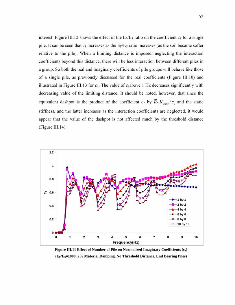
52
interest. Figure III.12 shows the effect of the EP/ES ratio on the coefficient c1 for a single
pile. It can be seen that c1 increases as the EP/ES ratio increases (as the soil became softer
relative to the pile). When a limiting distance is imposed, neglecting the interaction
coefficients beyond this distance, there will be less interaction between different piles in
a group. So both the real and imaginary coefficients of pile groups will behave like those
of a single pile, as previously discussed for the real coefficients (Figure III.10) and
illustrated in Figure III.13 for c1. The value of c1above 1 Hz decreases significantly with
decreasing value of the limiting distance. It should be noted, however, that since the
equivalent dashpot is the product of the coefficient c1 by /static sR K ci and the static
stiffness, and the latter increases as the interaction coefficients are neglected, it would
appear that the value of the dashpot is not affected much by the threshold distance
(Figure III.14).
0
0.2
0.4
0.6
0.8
1
1.2
0 1 2 3 4 5 6 7 8 9 10Frequency(Hz)
c 1
1 by 12 by 24 by 46 by 68 by 810 by 10
Figure III.11 Effect of Number of Pile on Normalized Imaginary Coefficients (c1)
(EP/ES=1000, 2% Material Damping, No Threshold Distance, End Bearing Piles)

53
0
0.2
0.4
0.6
0.8
1
1.2
0 1 2 3 4 5 6 7 8 9 10Frequency(Hz)
c 1Ep=100EsEp=500EsEp=1000Es
Figure III.12 Effect of EP/ES on Normalized Imaginary Coefficients (c1) of Single Pile
(ES=Constant=5E7, 2% Material Damping, No Threshold Distance, End Bearing Piles)
0
0.2
0.4
0.6
0.8
1
1.2
0 1 2 3 4 5 6 7 8 9 10
Frequency(Hz)
c 1
NO LIMITSmax=10DSmax=5D
Figure III.13 Effect of Smax on Imaginary Stiffness Coefficients of a 6 by 6 Pile Group
(EP=1000ES=5E10, 2% Material Damping, End Bearing Piles)
54
0.00E+00
1.00E+08
2.00E+08
3.00E+08
4.00E+08
5.00E+08
6.00E+08
7.00E+08
8.00E+08
9.00E+08
0 1 2 3 4 5 6 7 8 9 10Frequency(Hz)
Equi
vale
nt D
ashp
ot C
onst
ant (
N .
s/m
)
NO LIMITSmax=10DSmax=5D
Figure III.14 Effect of Smax on Equivalent Dashpot Constant of a 6 by 6 Pile Group
(EP=1000ES=5E10, 2% Material Damping, End Bearing Piles)
3.2.2 Vertical Stiffness
The vertical stiffness can also be expressed in the general form of Equation III.7. Unlike
the horizontal cases in which the results are insensitive to the pile length and the tip
conditions for most practical cases, the vertical stiffness is sensitive to the pile length
and boundary conditions at the pile end , so in this section we consider primarily the
vertical stiffness of floating piles and only that of end bearing piles for static loads.
(1) Static Stiffness
The group factor for the vertical stiffness is defined in the same way as for the horizontal
stiffness by Equation III.8, except that GK and SK represent the static vertical group
stiffness and static vertical stiffness of a single pile, respectively.

55
0.45
0.360.34 0.35
0.24
0.45
0.210.18
0.16 0.15
0.45
0.19
0.130.10
0.08
0.00
0.10
0.20
0.30
0.40
0.50
0 1 2 3 4 5 6 7 8 9 10Frequency (Hz)
Gro
up F
acto
r
Smax=5DSmax=10DNO LIMIT
Figure III.15 Vertical Static Group Factors for Vertical Stiffness
(EP/ES=1000, Floating Piles)
The vertical group factors of floating and end bearing piles are illustrated in Figures
III.15 & III.16 with the ratio of Young’s modulus of the piles to that of the soil (EP/ES)
equal to 1000. The vertical group factors are much larger than1/ N for end bearing piles
as shown in Figure III.16, but a little smaller than 1/ N for floating piles as shown in
Figure III.15. The reason is that, unlike the horizontal static stiffness, the vertical static
stiffness will increase substantially as the pile length increases and rigid rock is reached.
For end bearing piles there will be a lower bound for the vertical stiffness corresponding
to a value of ES equal to 0. In this case the total stiffness will be proportional to the
number of piles.
The limiting distance has the same effect on vertical group factors as on the horizontal
ones. The limit distance decreases the interaction between different piles in a pile group,
so the group factors increase substantially. The vertical group factors of end bearing
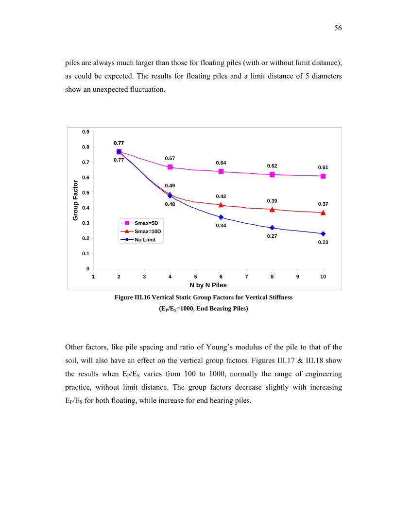
56
piles are always much larger than those for floating piles (with or without limit distance),
as could be expected. The results for floating piles and a limit distance of 5 diameters
show an unexpected fluctuation.
0.77
0.670.64 0.62 0.61
0.77
0.49
0.420.39 0.37
0.77
0.48
0.34
0.270.23
0
0.1
0.2
0.3
0.4
0.5
0.6
0.7
0.8
0.9
1 2 3 4 5 6 7 8 9 10N by N Piles
Gro
up F
acto
r
Smax=5DSmax=10DNo Limit
Figure III.16 Vertical Static Group Factors for Vertical Stiffness
(EP/ES=1000, End Bearing Piles)
Other factors, like pile spacing and ratio of Young’s modulus of the pile to that of the
soil, will also have an effect on the vertical group factors. Figures III.17 & III.18 show
the results when EP/ES varies from 100 to 1000, normally the range of engineering
practice, without limit distance. The group factors decrease slightly with increasing
EP/ES for both floating, while increase for end bearing piles.

57
0.45
0.19
0.130.1
0.08
0.47
0.21
0.140.11
0.09
0.55
0.27
0.180.14
0.12
0
0.1
0.2
0.3
0.4
0.5
0.6
0 1 2 3 4 5 6 7 8 9 10Frequency (Hz)
Gro
up F
acto
r
Ep=1000EsEp=500EsEp=100Es
Figure III.17 Effect of EP/ES on Vertical Group Factors
(No Threshold Distance, Floating Piles)
0.77
0.47
0.34
0.270.23
0.69
0.38
0.260.2
0.17
0.6
0.31
0.210.17
0.14
0
0.1
0.2
0.3
0.4
0.5
0.6
0.7
0.8
0.9
1 2 3 4 5 6 7 8 9 10
N by N Piles (Hz)
Gro
up F
acto
r
Ep=1000EsEp=500EsEp=100Es
Figure III.18 Effect of EP/ES on Vertical Group Factors
(No Threshold Distance, End Bearing Piles)

58
(2) Real and Imaginary Stiffness Coefficients
-20
-15
-10
-5
00 1 2 3 4 5 6 7 8 9 10
Frequency (Hz)
k 1 1 by 12 by 24 by 46 by 68 by 810 by 10
Figure III.19 Effect of Number of Piles on Real Coefficients
(EP=1000ES=5E10, 2% Material Damping, No Threshold Distance, Floating Piles)
The real coefficient 1k of a single pile is nearly a constant for all frequencies with a dip at
the dilatational natural frequency of the soil deposit (about 1.0 Hz in this case) for the
assumed Poisson’s ratio of 0.25. As the number of piles increases the coefficient 1k
exhibits a parabolic variation with frequency like that of the horizontal stiffness, as
illustrated in Figure III.19, but with smaller fluctuations around the second degree
parabola.
Using the same method described earlier, one can find an equivalent mass for the
vertical case. The results of LSF (Least Square Fit) for the vertical stiffness of floating

59
piles are shown in Figure III.20. For a single pile, the equivalent mass is essentially zero.
As the number of piles increases, the equivalent mass increases and is proportional
to 2( 1)N − , as illustrated in Figure III.21, which suggests that the equivalent mass for
vertical vibration of floating pile groups is proportional to the equivalent area (as for the
horizontal case).
0 2 4 6 8 10-1
0
1
2
Frequency(Hz)
k1
0 2 4 6 8 10-2
-1
0
1
Frequency(Hz)
k1
0 2 4 6 8 10-20
-15
-10
-5
0
5
Frequency(Hz)
k1
0 2 4 6 8 10-40
-30
-20
-10
0
10
Frequency(Hz)
k1
0 2 4 6 8 10-60
-40
-20
0
20
Frequency(Hz)
k1
0 2 4 6 8 10-80
-60
-40
-20
0
20
Frequency(Hz)
k1
k1 of Single PileLeast Square Fit
k1 of 2 by 2 Pile GroupsLeast Square Fit
k1 of 4 by 4 Pile GroupsLeast Square Lit
k1 of 6 by 6 Pile GroupsLeast Square Fit
k1 of 8 by 8 Pile GroupsLeast Square Fit
k1 of 10 by 10 Pile GroupsLeast Square Fit
Figure III.20 LSF of Equivalent Mass of Vertical Stiffness

60
Y = 6.67*105*(N-1)2
0.00E+00
1.00E+07
2.00E+07
3.00E+07
4.00E+07
5.00E+07
6.00E+07
0 1 2 3 4 5 6 7 8 9 10N by N Piles
Equi
vale
nt M
ass
(kg)
Equivalent Mass
Figure III.21 Equivalent Mass with Number of Piles
Figure III.22 shows the variation of the real coefficient 1k with frequency for a 6 by 6
pile group when a limit distance is imposed. It can be seen that the introduction of a limit
distance of 5 or even 10 diameters will decrease the fluctuation, leading to a variation
very similar to that of a smaller pile group with smaller equivalent mass, which results
from the reduction of interaction between different piles.
The imaginary stiffness coefficients 1c of floating piles for different number of piles,
shown in Figure III.23, remain zero below the fundamental frequency in dilatation
compression (about 1 Hz in this case), then jump suddenly and decrease to a constant
value for a single pile, but are nearly a constant for pile groups in the normal range of
interest. Figure III.24 shows the coefficients 1c of single floating piles for different
values of the EP/ES ratio. The coefficient 1c for a single pile decreases with decreasing
EP/ES.

61
-7
-6
-5
-4
-3
-2
-1
0
1
2
0 1 2 3 4 5 6 7 8 9 10
Frequency (Hz)
k 1
Smax=5DSmax=10DNO LIMIT
Figure III.22 Effect of Threshold Distance on Real Coefficients of 6 by 6 Pile Groups
(EP=1000ES=5E10, 2% Material Damping, Floating Piles)
0
0.5
1
1.5
2
2.5
3
3.5
4
0 1 2 3 4 5 6 7 8 9 10
Frequency (Hz)
c 1
1 by 12 by 24 by 46 by 68 by 810 by 10
Figure III.23 Effect of Number of Piles on Imaginary Coefficients
(EP=1000ES=5E10, 2% Material Damping, No Threshold Distance, Floating Piles)

62
The effect of imposing a limit distance on the interaction coefficients in the imaginary
coefficient 1c is similar to that discussed earlier for the horizontal case, the coefficient
decreasing with decreasing limit distance. The same observations made earlier apply
here. Although the coefficient decreases the static stiffness increases so that the
equivalent dashpot may not change very much.
0
0.5
1
1.5
2
2.5
3
3.5
4
0 1 2 3 4 5 6 7 8 9 10Frequency (Hz)
c 1
Ep=100EsEp=500EsEp=1000Es
Figure III.24 Effect of EP/ES on Imaginary Coefficients of Single Piles
(ES=Constant=5E10, 2% Material Damping, No Threshold Distance, Floating Piles)
3.2.3 Rocking Stiffness
As in the vertical case the rocking stiffness is affected significantly by the length and tip
condition of the piles, since it is a function of the vertical stiffness of each pile. Only the
dynamic case of floating piles is studied in this section. End bearing piles are considered
for the static case for comparison purposes.

63
(1) Static Stiffness
The definition of the static group reduction factor the for rocking stiffness is
2
1
GRocking n
S ii
KGFK d
=
=
∑i
where
n ……………………………….……………………………………...… number of piles;
id …………………………...….....distance from i -th pile to the center of the pile group;
GK …………………………….………………...static rocking stiffness of the pile group;
SK …………………………..……………..……...static vertical stiffness of a single pile.
1.56
1.33
0.36 0.370.29
1.56
0.58
0.360.27 0.22
1.56
0.69
0.39
0.260.20
0.0
0.2
0.4
0.6
0.8
1.0
1.2
1.4
1.6
1.8
0 1 2 3 4 5 6 7 8 9 10Frequency (Hz)
Gro
up F
acto
r
Smax=5DSmax=10DNO LIMIT
Figure III.25 Static Group Reduction Factor for Rocking Stiffness
(EP/ES=1000, Floating Piles)

64
Figures III.25 & III.26 show the group factor for the rocking stiffness of floating piles
and end bearing piles, respectively, with EP/ES=1000. The group factor is larger than 1
for 2 by 2 pile groups, which implies the interaction between piles will increase the
group static stiffness, while smaller than 1 for pile groups larger than 4 by 4.
With the introduction of a limiting distance, the group factor of end bearing piles will
decrease for smaller pile groups while increasing for larger groups. The group factor of
floating piles for max 10S D= is almost the same as that without limit distance, while that
for max 5S D= exhibits some unexpected fluctuations more pronounced for small pile
groups.
1.1
0.80.72
0.68 0.66
1.1
0.86
0.61
0.520.47
1.1
0.92
0.72
0.57
0.46
0
0.2
0.4
0.6
0.8
1
1.2
0 2 4 6 8 10N by N Piles
Gro
up F
acto
r
Smax=5DSmax=10DNo Limit
Figure III.26 Static Group Reduction Factor for Rocking Stiffness
(EP/ES=1000, End Bearing Piles)

65
0.69
0.39
0.260.2
0.71
0.41
0.280.21
0.75
0.48
0.340.26
1.561.49
1.31
0
0.2
0.4
0.6
0.8
1
1.2
1.4
1.6
1.8
0 1 2 3 4 5 6 7 8 9 10Frequency (Hz)
Gro
up F
acto
r
Ep=1000Es
Ep=500Es
Ep=100Es
Figure III.27 Effect of EP/ES on Static Group Factor
(No Threshold Distance, Floating Piles)
0.92
0.72
0.57
0.46
0.88
0.63
0.47
0.37
0.79
0.53
0.380.3
1.11.151.24
0
0.2
0.4
0.6
0.8
1
1.2
0 1 2 3 4 5 6 7 8 9 10N by N Piles
Gro
up F
acto
r
Ep=1000EsEp=500EsEp=100Es
Figure III.28 Effect of EP/ES on Static Group Factor
(No Threshold Distance, End Bearing Piles)

66
The group factor also depends on other factors, like EP/ES, as shown in Figures III.27 &
III.28. All curves in the two figures intersect at about 3N = (It depends on pile spacing.).
As EP/ES increases, the group factors decrease for 2 by 2 pile groups and increase for
larger groups.
The group factors of end bearing piles are larger than those of floating piles for larger
pile groups while smaller for 2 by 2 groups.
(2) Real and Imaginary Stiffness Coefficients
-6
-5
-4
-3
-2
-1
0
1
2
0 1 2 3 4 5 6 7 8 9 10
Frequency (Hz)
k 1
2 by 24 by 46 by 68 by 810 by 10
Figure III.29 Effect of Number of Piles on Real Coefficients
(EP=1000ES=5E10, 2% Material Damping, No Threshold Distance, Floating Piles)
The real stiffness coefficient 1k of the rocking stiffness, shown in Figure III.29, behaves
like that of the single degree of freedom system in Figure III.7. Unlike the real

67
coefficient 1k of the horizontal stiffness, 1k of the rocking stiffness does not have large
fluctuations even for large pile groups like 10 by 10. One can also fit (Least Square Fit)
the coefficients 1k by an expression of the form 21 b ω− ⋅ to find an equivalent mass
moment of inertia ( eq staticI K b= i ), as in the case of horizontal and vertical stiffness.
Figure III.30 Least Square Fit of Equivalent Inertia of Rotation of Rocking Stiffness

68
Y = 7.75*105*(N-2)4
0.00E+00
5.00E+08
1.00E+09
1.50E+09
2.00E+09
2.50E+09
3.00E+09
3.50E+09
0 1 2 3 4 5 6 7 8 9 10N by N Piles
Equi
vale
nt In
ertia
of R
otat
ion
(kg*
m2 )
Equivalent Inertia of Rotation
Figure III.31 Equivalent Inertia of Rotation with Number of Piles
Figure III.30 shows the results of the LSF (Least Square Fit) for the real coefficient 1k .
It can be seen that one can approximate the coefficient 1k of the rocking stiffness by a
second degree parabola of the form of 21 b ω− ⋅ and the equivalent moment of inertia is
proportional to 4( 2)N − , as illustrated in Figure III.31. This is very similar to a
cylindrical rigid mass, whose rotational inertia is proportional to the radius to the fourth
order.
The introduction of a limiting distance will lead to an even smoother variation with
frequency and decrease in the curvature of the second degree parabola, as illustrated in
Figure III.32, indicating a smaller equivalent mass vibrating in phase with the
foundation, but the reduction is not as marked as for the horizontal stiffness.

69
-6
-5
-4
-3
-2
-1
0
1
2
0 1 2 3 4 5 6 7 8 9 10
Frequency (Hz)
k 1
Smax=5DSmax=10DNO LIMIT
Figure III.32 Effect of Limit Distance on Real Coefficients of 6 by 6 Pile Groups
(EP=1000ES=5E10, 2% Material Damping, Floating Piles)
Figure III.33 shows the imaginary coefficient 1c of the rocking stiffness for different
number of piles. The coefficient 1c jumps at 1 Hz and keeps increasing slowly and
smoothly for 2 by 2, 4 by 4 and 6 by 6 pile groups, while it oscillates around a constant
(about 0.4 in this case) for 8 by 8 and 10 by 10 pile groups. It can be seen that the
coefficient 1c of a 2 by 2 pile group is much smaller than that of larger pile groups.
The effect of EP/ES on the imaginary coefficient 1c for a 2 by 2 pile group is illustrated
in Figure III.34. For EP/ES varying from 100 to 1000 in the normal range of engineering
practice, 1c increases a little bit for increasing EP/ES but the shape of the curves is very
similar.

70
0
0.1
0.2
0.3
0.4
0.5
0.6
0 1 2 3 4 5 6 7 8 9 10Frequency (Hz)
c 12 by 24 by 46 by 68 by 810 by 10
Figure III.33 Effect of Number of Piles on Imaginary Coefficients
(EP=1000ES=5E10, 2% Material Damping, No Threshold Distance, Floating Piles)
0
0.05
0.1
0.15
0.2
0.25
0.3
0 1 2 3 4 5 6 7 8 9 10Frequency (Hz)
c 1
Ep=100EsEp=500EsEp=1000Es
Figure III.34 Effect of EP/ES on Imaginary Coefficients of 2 by 2 Pile Groups
(2% Material Damping, No Threshold Distance, Floating Piles)

71
CHAPTER IV
DYNAMIC STIFFNESS OF FOUNDATIONS OF MARGA-MARGA
BRIDGE’S PIERS
In this chapter, the procedures described in the previous one are applied to determine the
dynamic stiffness of the pile foundations of piers P2 to P6 of the Marga-Marga bridge.
The stiffness of the foundations for piers P1 and P7 were determined with an existing
program for mat foundations.
4.1 Introduction
The Marga-Marga bridge, shown schematically in Figure IV.1, has seven piers (P1~P7),
five of them (P2~P6) with pile foundations. Each of the pile foundations consists of a 5
by 2 pile group (rows of 5 piles in the direction perpendicular to the figure and 2 in the
longitudinal direction of the bridge). Piers P1 and P7 have surface mat foundations
without any supporting piles.
Figure IV. 1 Piers and Pile Groups of Marga-Marga Bridge

72
To calculate the stiffness of these pile groups, the interaction between two different pile
groups was neglected, assuming each pile group embedded in a horizontal layered soil
deposit extending to infinity in the two horizontal directions, based on the fact that the
distance between pile groups is much larger than the horizontal dimension of the pile
groups themselves.
4.2 Dimensions of the Pile Groups and Soil Properties
The dimensions of the piers and their pile foundations are illustrated in Figure IV.2 and
Table IV.1. For piers P2~P6, which have pile foundations, the dimensions of the caps
are the same,13.5 5× m. The pile spacings in the x and y directions are 3 and 4 meters
respectively, as illustrated in Figure IV.3. The length and diameter of the piles are listed
in Table IV.2.
Figure IV. 2 A Pier and Its Pile Foundation

73
Table IV. 1 Dimension of the Pier and Cap
Pier # H
(m)
H1
(m)
Width of Cap
(m)
1 21.865 1.5 10.5
2 26.317 2.0 13.5
3 27.138 2.0 13.5
4 26.260 2.0 13.5
5 26.082 2.0 13.5
6 30.154 2.0 13.5
7 30.086 1.5 10.5
Y
X
Figure IV. 3 Dimensions of Cap and Pile Spacing
The soil properties under each pier, including the thickness of each layer and its shear
wave velocity, are shown in Tables IV.3 to IV.6. The soil under the dashed line at the
bottom of Figure IV.1 is assumed to have a shear wave velocity of 550 m/s, while the
layers above the line have shear wave velocities in the range of 200~400 m/s. All the

74
soils are assumed to have a Poisson’s ratio, mass density and internal damping of 0.25,
2000 kg/m3 and 5%, respectively.
Table IV. 2 Length and Diameter of Piles
Pier #L
(m)
Diameter
(m)
2 19.50 1.0
3 30.00 1.0
4 15.06 1.0
5 14.02 1.0
6 31.70 1.0
Table IV. 3 Soil Properties for Pier #2
Thickness
(m)
Depth
(m)
Shear Wave
Velocity (m/s)
Layer 1 7.20 7.20 240
Layer 2 5.00 12.20 210
Layer 3 27.80 40.00 550
Layer 4 50.00 90.00 550
The piles are made of concrete with a Young’s modulus of about 103 10× Pa. The mass
density and internal damping are assumed to be 2500kg/m3 and 5%, respectively. This
represents an EP/ES ratio of 75 to 100, indicating a stiffer soil than the one normally
encountered with pile foundations.
No limiting distance was used in the calculation of the dynamic stiffness terms.

75
Table IV. 4 Soil Properties for Pier #3 and #4
Thickness
(m)
Depth
(m)
Shear Wave
Velocity (m/s)
Layer 1 7.20 7.20 240
Layer 2 5.00 12.20 210
Layer 3 4.69 16.89 330
Layer 4 13.11 30.00 360
Layer 5 10.00 40.00 390
Layer 6 50.00 90.00 550
Table IV. 5 Soil Properties for Pier #5
Thickness
(m)
Depth
(m)
Shear Wave
Velocity (m/s)
Layer 1 7.20 7.20 240
Layer 2 5.00 12.20 310
Layer 3 4.69 16.89 330
Layer 4 13.11 30.00 360
Layer 5 10.00 40.00 390
Layer 6 50.00 90.00 550

76
Table IV. 6 Soil Properties for Pier #6
Thickness
(m)
Depth
(m)
Shear Wave
Velocity (m/s)
Layer 1 1.35 1.35 240
Layer 2 5.00 6.35 310
Layer 3 4.69 11.04 330
Layer 4 13.11 24.15 210
Layer 5 10.00 35.15 390
Layer 6 50.00 84.15 550
4.3 Dynamic Stiffness of Pile Foundations
The dynamic stiffness terms (real and imaginary parts) were computed by the programs
described in the previous chapter using the data shown above. Figures IV.4 to IV.13
show the dynamic stiffness of the pile foundations P2~P6.
The real and imaginary parts of the horizontal dynamic stiffness in the X and Y
directions are shown in Figures IV.4 to IV.7. The horizontal stiffness is similar in the
two directions and slightly larger in the longitudinal direction of the bridge, because
group effects are less important in this direction (only rows of 2 piles instead of 5). Since
the horizontal stiffness depends only on the soil and pile properties near the surface,
those of P3 and P4 are almost the same, though the length of the piles in the two groups
is very different (P3 has piles 30m long but those of P4 are only 15.06m long).
The real part of the horizontal stiffness is nearly constant, with some oscillations. The
real part of the horizontal stiffness for pier P6 is the largest of the five with an apparent
dip at the fundamental natural frequency in shear (about 1.4 Hz in this case), which
results from the stiffer soil near the surface (Table IV.6).
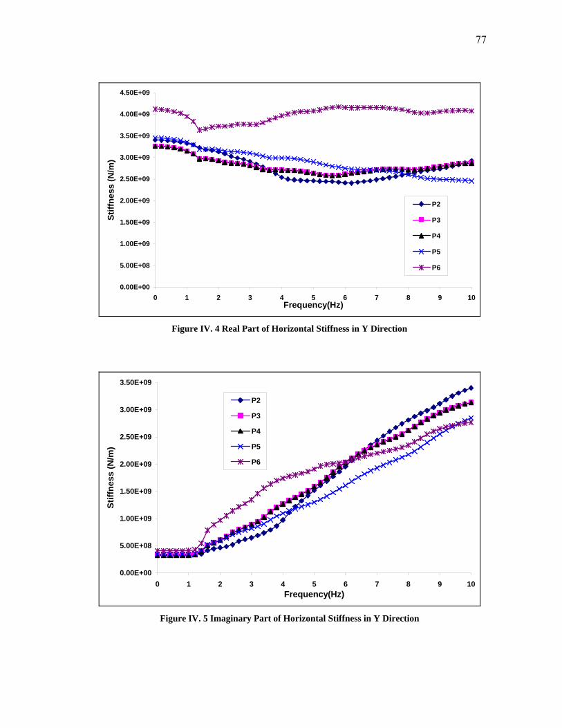
77
0.00E+00
5.00E+08
1.00E+09
1.50E+09
2.00E+09
2.50E+09
3.00E+09
3.50E+09
4.00E+09
4.50E+09
0 1 2 3 4 5 6 7 8 9 10Frequency(Hz)
Stiff
ness
(N/m
)
P2
P3
P4
P5
P6
Figure IV. 4 Real Part of Horizontal Stiffness in Y Direction
0.00E+00
5.00E+08
1.00E+09
1.50E+09
2.00E+09
2.50E+09
3.00E+09
3.50E+09
0 1 2 3 4 5 6 7 8 9 10Frequency(Hz)
Stiff
ness
(N/m
)
P2
P3
P4
P5
P6
Figure IV. 5 Imaginary Part of Horizontal Stiffness in Y Direction

78
0.00E+00
5.00E+08
1.00E+09
1.50E+09
2.00E+09
2.50E+09
3.00E+09
3.50E+09
4.00E+09
4.50E+09
5.00E+09
0 1 2 3 4 5 6 7 8 9 10Frequency(Hz)
Stiff
ness
(N/m
)
P2
P3
P4
P5
P6
Figure IV. 6 Real Part of Horizontal Stiffness in X Direction
0.00E+00
5.00E+08
1.00E+09
1.50E+09
2.00E+09
2.50E+09
3.00E+09
3.50E+09
4.00E+09
0 1 2 3 4 5 6 7 8 9 10Frequency(Hz)
Stiff
ness
(N/m
)
P2
P3
P4
P5
P6
Figure IV. 7 Imaginary Part of Horizontal Stiffness in X Direction

79
0.00E+00
5.00E+08
1.00E+09
1.50E+09
2.00E+09
2.50E+09
3.00E+09
3.50E+09
4.00E+09
4.50E+09
0 1 2 3 4 5 6 7 8 9 10Frequency(Hz)
Stiff
ness
(N/m
)
P2
P3(P4)
P5
P6
Figure IV. 8 Real Part of Horizontal Stiffness of an Equivalent Surface Mat
0.00E+00
5.00E+08
1.00E+09
1.50E+09
2.00E+09
2.50E+09
3.00E+09
0 1 2 3 4 5 6 7 8 9 10Frequency(Hz)
Stiff
ness
(N/m
)
P2
P3(P4)
P5
P6
Figure IV. 9 Imaginary Part of Horizontal Stiffness of an Equivalent Surface Mat

80
0.00E+00
2.00E+09
4.00E+09
6.00E+09
8.00E+09
1.00E+10
1.20E+10
1.40E+10
0 1 2 3 4 5 6 7 8 9 10Frequency(Hz)
Stiff
ness
(N/m
)
P2
P3
P4
P5
P6
Figure IV. 10 Real Part of Vertical Stiffness
The imaginary parts are constant below the fundamental natural frequency in shear, with
a value representing the effect of the internal (material) damping, then increase almost
linearly with frequency.
As a matter of interest, Figures IV.8 & IV.9 show the horizontal stiffness for mat
foundations representing the cap of the pile groups for each pier. It can be seen that the
values are very similar to those of the pile foundations and just slightly smaller. In
comparing these values, the rectangular mats are replaced by an equivalent circular
foundation with the same area leading to the same value in both horizontal directions.
From the real parts of the vertical stiffness shown in Figure IV.10, one can identify the
dilatational fundamental frequency (2.4 Hz in this case). Basically, the real part
decreases slowly with frequency, except for P6. P2 has the largest static vertical stiffness
because the distance to the hard material is the smallest. The variation of the imaginary

81
parts of the vertical stiffness with frequency, shown in Figure IV.11, is very similar to
that of the horizontal stiffness with the difference in the threshold frequency for radiation
damping (from 1.4 to 2.4 Hz).
Figures IV.12 & IV.13 show the vertical stiffness of the pile caps by themselves. As
expected these values are much smaller than those of the pile groups by a factor of
almost 2.5.
The rocking stiffness, illustrated in Figure IV.14 to IV.17, has a much smoother
variation with frequency than either the horizontal or the vertical stiffness. It is hard to
identify from the figures for the real part the fundamental frequencies of the soil. The
real part decreases with frequency in the normal range of engineering practice. The real
parts of P2 and P6 are larger than those of the other piers, which implies that the rocking
stiffness is sensitive to both pile tip conditions and soil properties. The imaginary parts
follow the same shape as those of the horizontal and vertical stiffness but they have less
variation with frequency. As could be expected, the rocking stiffness around an axis
perpendicular to the longitudinal direction of the bridge is smaller than the stiffness
around the longitudinal axis by a factor of about 3.
Figures IV.18 to IV.21 show the rocking stiffness for the pile caps as surface
foundations (without piles). The equivalent circular foundations had the radii selected so
as to yield the same moment of inertia. Once again the pile foundations have a much
larger stiffness by a factor of about 4.

82
0.00E+00
2.00E+09
4.00E+09
6.00E+09
8.00E+09
1.00E+10
1.20E+10
1.40E+10
1.60E+10
1.80E+10
0 1 2 3 4 5 6 7 8 9 10Frequency(Hz)
Stiff
ness
(N/m
)P2
P3
P4
P5
P6
Figure IV. 11 Imaginary Part of Vertical Stiffness
0.00E+00
1.00E+09
2.00E+09
3.00E+09
4.00E+09
5.00E+09
6.00E+09
0 1 2 3 4 5 6 7 8 9 10Frequency(Hz)
Stiff
ness
(N/m
)
P2
P3(P4)
P5
P6
Figure IV. 12 Real Part of Vertical Stiffness of an Equivalent Surface Mat

83
0.00E+00
5.00E+08
1.00E+09
1.50E+09
2.00E+09
2.50E+09
3.00E+09
3.50E+09
4.00E+09
4.50E+09
5.00E+09
0 1 2 3 4 5 6 7 8 9 10Frequency(Hz)
Stiff
ness
(N/m
)
P2
P3(P4)
P5
P6
Figure IV. 13 Imaginary Part of Vertical Stiffness of an Equivalent Surface Mat
0.00E+00
5.00E+10
1.00E+11
1.50E+11
2.00E+11
2.50E+11
3.00E+11
3.50E+11
4.00E+11
0 1 2 3 4 5 6 7 8 9 10Frequency(Hz)
Stiff
ness
(N*m
)
P2
P3
P4
P5
P6
Figure IV. 14 Real Part of Rocking Stiffness around X Axis

84
0.00E+00
2.00E+10
4.00E+10
6.00E+10
8.00E+10
1.00E+11
1.20E+11
1.40E+11
1.60E+11
1.80E+11
2.00E+11
0 1 2 3 4 5 6 7 8 9 10Frequency(Hz)
Stiff
ness
(N*m
)
P2
P3
P4
P5
P6
Figure IV. 15 Imaginary Part of Rocking Stiffness around X Axis
0.00E+00
2.00E+10
4.00E+10
6.00E+10
8.00E+10
1.00E+11
1.20E+11
0 1 2 3 4 5 6 7 8 9 10Frequency(Hz)
Stiff
ness
(N*m
)
P2
P3
P4
P5
P6
Figure IV. 16 Real Part of Rocking Stiffness around Y Axis

85
0.00E+00
5.00E+09
1.00E+10
1.50E+10
2.00E+10
2.50E+10
3.00E+10
0 1 2 3 4 5 6 7 8 9 10Frequency(Hz)
Stiff
ness
(N*m
)
P2
P3
P4
P5
P6
Figure IV. 17 Imaginary Part of Rocking Stiffness around Y Axis
0.00E+00
2.00E+10
4.00E+10
6.00E+10
8.00E+10
1.00E+11
1.20E+11
1.40E+11
1.60E+11
1.80E+11
0 1 2 3 4 5 6 7 8 9 10Frequency(Hz)
Stiff
ness
(N*m
)
P2
P3(P4)
P5
P6
Figure IV. 18 Real Part of Rocking Stiffness around X Axis of an Equivalent Surface Mat

86
0.00E+00
1.00E+10
2.00E+10
3.00E+10
4.00E+10
5.00E+10
6.00E+10
0 1 2 3 4 5 6 7 8 9 10Frequency(Hz)
Stiff
ness
(N*m
)
P2
P3(P4)
P5
P6
Figure IV. 19 Imaginary Part of Rocking Stiffness around X Axis of an Equivalent Surface Mat
0.00E+00
5.00E+09
1.00E+10
1.50E+10
2.00E+10
2.50E+10
3.00E+10
3.50E+10
4.00E+10
4.50E+10
0 1 2 3 4 5 6 7 8 9 10Frequency(Hz)
Stiff
ness
(N*m
)
P2
P3(P4)
P5
P6
Figure IV. 20 Real Part of Rocking Stiffness around Y Axis of an Equivalent Surface Mat

87
0.00E+00
1.00E+09
2.00E+09
3.00E+09
4.00E+09
5.00E+09
6.00E+09
7.00E+09
8.00E+09
9.00E+09
0 1 2 3 4 5 6 7 8 9 10Frequency(Hz)
Stiff
ness
(N*m
)P2
P3(P4)
P5
P6
Figure IV. 21 Imaginary Part of Rocking Stiffness around Y Axis of an Equivalent Surface Mat
P1 and P7 only have surface mats without supporting piles. One can find an equivalent
circular mat (having the same area as the rectangular mat shown in Figure IV.3) to
calculate their horizontal stiffness (the same in the two directions) and vertical stiffness,
while using a circle having the same moment of inertia as the rectangular mat to
calculate the rocking stiffness. Results are shown in Figure IV.22, assuming that the
subsoil is 90 meters deep with a shear wave velocity of 550m/s.
It can be seen that the natural frequency in shear is about 1.6 Hz and the dilatational
natural frequency is about 2.5 Hz for this case.

88
0 2 4 6 8 100
0.5
1
1.5
2x 10
10
Frequency (Hz)
Hor
izon
tal S
riffn
ess
in Y
Dire
ctio
n (N
/m)
0 2 4 6 8 100
0.5
1
1.5
2x 10
10
0 2 4 6 8 100
0.5
1
1.5
2x 10
10
0 2 4 6 8 100
2
4
6
8x 10
11
0 2 4 6 8 100
0.5
1
1.5
2x 10
11
RealImaginary
RealImaginary
RealImaginary
RealImaginary
RealImaginary
Frequency (Hz)
Hor
izon
tal S
riffn
ess
in X
Dire
ctio
n (N
/m)
Ver
tical
Srif
fnes
s (
N/m
) R
ocki
ng S
riffn
ess
arou
nd X
Axi
s (N
*m)
Roc
king
Srif
fnes
s ar
ound
Y A
xis
(N*m
)
Frequency (Hz)
Frequency (Hz) Frequency (Hz) Figure IV. 22 Stiffness of Surface Mat of Pier #1 and Pier #7
4.4 Dynamic Stiffness with Reduced Soil Shear Modulus
To study further the potential SSI effects, the shear wave velocities were reduced over
the top 12 meters to simulate some nonlinear soil behavior. Other properties of the soils
are the same as used before. The foundation stiffness terms were calculated again for this
case. The assumed properties and the calculated foundation stiffness are shown in Tables
IV.7 - IV.10 and Figures IV.23 - IV.33.

89
Table IV. 7 Reduced Soil Properties for Pier #2
Thickness
(m)
Depth
(m)
Shear Wave
Velocity (m/s)
Layer 1 7.20 7.20 150
Layer 2 5.00 12.20 150
Layer 3 27.80 40.00 550
Layer 4 50.00 90.00 550
Table IV. 8 Reduced Soil Properties for Pier #3 and #4
Thickness
(m)
Depth
(m)
Shear Wave
Velocity (m/s)
Layer 1 7.20 7.20 150
Layer 2 5.00 12.20 150
Layer 3 4.69 16.89 330
Layer 4 13.11 30.00 360
Layer 5 10.00 40.00 390
Layer 6 50.00 90.00 550
Table IV. 9 Reduced Soil Properties for Pier #5
Thickness
(m)
Depth
(m)
Shear Wave
Velocity (m/s)
Layer 1 7.20 7.20 150
Layer 2 5.00 12.20 150
Layer 3 4.69 16.89 330
Layer 4 13.11 30.00 360
Layer 5 10.00 40.00 390
Layer 6 50.00 90.00 550

90
Table IV. 10 Reduced Soil Properties for Pier #6
Thickness
(m)
Depth
(m)
Shear Wave
Velocity (m/s)
Layer 1 1.35 1.35 150
Layer 2 5.00 6.35 150
Layer 3 4.69 11.04 150
Layer 4 13.11 24.15 210
Layer 5 10.00 35.15 390
Layer 6 50.00 84.15 550
The new horizontal stiffness in both directions decreases by 50% because it depends on
the properties of the soil near the surface, while the new rocking stiffness decreases by
about 20%~30%. Only the vertical stiffness is almost the same as before. The shapes of
the curves of the dynamic stiffness with frequency are very similar to those obtained
before. The natural frequency in shear has been reduced from 1.6Hz to 1.4Hz while the
dilatational natural frequency is almost the same as before.

91
0.00E+00
5.00E+08
1.00E+09
1.50E+09
2.00E+09
2.50E+09
0 1 2 3 4 5 6 7 8 9 10Frequency(Hz)
Stiff
ness
(N/m
)
P2
P3
P4
P5
P6
Figure IV. 23 New Real Part of Horizontal Stiffness in X Direction
0.00E+00
5.00E+08
1.00E+09
1.50E+09
2.00E+09
2.50E+09
3.00E+09
3.50E+09
0 1 2 3 4 5 6 7 8 9 10Frequency(Hz)
Stiff
ness
(N/m
)
P2
P3
P4
P5
P6
Figure IV. 24 New Imaginary Part of Horizontal Stiffness in X Direction

92
0.00E+00
2.00E+08
4.00E+08
6.00E+08
8.00E+08
1.00E+09
1.20E+09
1.40E+09
1.60E+09
1.80E+09
2.00E+09
0 1 2 3 4 5 6 7 8 9 10Frequency(Hz)
Stiff
ness
(N/m
)
P2
P3
P4
P5
P6
Figure IV. 25 New Real Part of Horizontal Stiffness in Y Direction
0.00E+00
5.00E+08
1.00E+09
1.50E+09
2.00E+09
2.50E+09
0 1 2 3 4 5 6 7 8 9 10Frequency(Hz)
Stiff
ness
(N/m
)
P2
P3
P4
P5
P6
Figure IV. 26 New Imaginary Part of Horizontal Stiffness in Y Direction

93
0.00E+00
2.00E+09
4.00E+09
6.00E+09
8.00E+09
1.00E+10
1.20E+10
1.40E+10
0 1 2 3 4 5 6 7 8 9 10Frequency(Hz)
Stiff
ness
(N/m
)
P2
P3
P4
P5
P6
Figure IV. 27 New Real Part of Vertical Stiffness
0.00E+00
2.00E+09
4.00E+09
6.00E+09
8.00E+09
1.00E+10
1.20E+10
1.40E+10
1.60E+10
0 1 2 3 4 5 6 7 8 9 10Frequency(Hz)
Stiff
ness
(N/m
)
P2
P3
P4
P5
P6
Figure IV. 28 New Imaginary Part of Vertical Stiffness

94
0.00E+00
5.00E+10
1.00E+11
1.50E+11
2.00E+11
2.50E+11
3.00E+11
3.50E+11
0 1 2 3 4 5 6 7 8 9 10Frequency(Hz)
Stiff
ness
(N*m
)
P2
P3
P4
P5
P6
Figure IV. 29 New Real Part of Rocking Stiffness around X Axis
0.00E+00
2.00E+10
4.00E+10
6.00E+10
8.00E+10
1.00E+11
1.20E+11
1.40E+11
1.60E+11
1.80E+11
2.00E+11
0 1 2 3 4 5 6 7 8 9 10Frequency(Hz)
Stiff
ness
(N*m
)
P2
P3
P4
P5
P6
Figure IV. 30 New Imaginary Part of Rocking Stiffness around X Axis

95
0.00E+00
1.00E+10
2.00E+10
3.00E+10
4.00E+10
5.00E+10
6.00E+10
7.00E+10
8.00E+10
9.00E+10
0 1 2 3 4 5 6 7 8 9 10Frequency(Hz)
Stiff
ness
(N*m
)
P2
P3
P4
P5
P6
Figure IV. 31 New Real Part of Rocking Stiffness around Y Axis
0.00E+00
5.00E+09
1.00E+10
1.50E+10
2.00E+10
2.50E+10
0 1 2 3 4 5 6 7 8 9 10Frequency(Hz)
Stiff
ness
(N*m
)
P2
P3
P4
P5
P6
Figure IV. 32 New Imaginary Part of Rocking Stiffness around Y Axis

96
Figure IV. 33 New Stiffness of Mat under Pier #1 and Pier #7

97
CHAPTER V
EFFECT OF RUBBER PADS’ STIFFNESS
The formulation and computer software described in Chapter II were applied to the
Marga-Marga bridge to estimate its frequency response characteristics due to base
motions, ignoring first soil-structure interaction effects. The main objective was to study
the effect of the stiffness of the rubber pads on the dynamic response of the bridge.
5.1 Properties of Structure
5.1.1 Deck
The Marga-Marga bridge is shown schematically in Figure V.1.
Figure V. 1 Overview of Marga-Marga Bridge
The deck of the bridge consists of 8 spans, which are all 50 meters long except the span
connecting the north abutment and pier 1, which is 33 meters long. The deck is
composite with a concrete slab over 4 steel I-beams. It is modeled as an equivalent beam
with a mass density, Poisson’s ratio and Young’s modulus of 2940kg/m3, 0.245 and

98
103.3 10× Pa, respectively. The centroid of the equivalent beam cross section is 2.65
meters above the top of the base isolators (rubber pads) and 0.45 meters below the upper
surface (as shown in Figure V.2).
CentroidSteel Girders
Concrete Slab
Y
Z
Figure V. 2 Cross Section of Deck
The properties of the deck cross section are:
2
2
4
2
4
4
8.13(m )3.85(m )
238.6(m )
2.25(m )
5.98(m )
0.116(m )
sy
z
sz
y
AA
I
A
I
J
⎧ =⎪
=⎪⎪ =⎪⎨
=⎪⎪ =⎪⎪ =⎩
in which A is the area of the deck’s cross section; syA and szA are the shear areas of the
composite cross section in the Y and Z direction, respectively; zI and yI are the bending
moments of inertia in the Z and Y direction, respectively, and J is the torsional moment
of inertia.

99
5.1.2 Piers
The piers and their dimensions are illustrated in Figure V.3. The formulation of the
dynamic stiffness of prismatic members assumes a constant cross section. Each pier was
therefore divided into three members according to the variation of the cross section.
As shown in Figures V.3 and V.4, the top and bottom parts (members) are solid, while
the long member in between is hollow. The mass density, Poisson’s ratio and Young’s
modulus used in the analysis for the piers are 2500 kg/m3, 0.2 and 103.3 10× Pa,
respectively.
Figure V. 3 Transverse View of Pier and Its Dimensions
Pier # H
(m)
H1
(m)
B
(m)
1 21.865 1.5 10.5
2 26.317 2.0 13.5
3 27.138 2.0 13.5
4 26.260 2.0 13.5
5 26.082 2.0 13.5
6 30.154 2.0 13.5
7 30.086 1.5 10.5

100
The properties of the pier cross sections are:
2
2
4
2
4
4
31.6(m )26.86(m )
657.385(m )
26.86(m )
10.533(m )
37.92(m )
sy
x
sx
y
AA
I
A
I
J
⎧ =⎪
=⎪⎪ =⎪⎨
=⎪⎪ =⎪⎪ =⎩
and
2
2
4
2
4
4
6.38(m )4.17(m )
63.33(m )
1.25(m )
4.18(m )
12.658(m )
sy
z
sz
y
AA
I
A
I
J
⎧ =⎪
=⎪⎪ =⎪⎨
=⎪⎪ =⎪⎪ =⎩
for the top member and the middle member, respectively.
X
Y
Figure V. 4 Cross Sections of Pier

101
The properties of the bottom members’ cross-sections are:
2
2
4
2
4
4
74.25(m )63.113(m )
1127.672(m )
63.113(m )
187.172(m )
552.531(m )
sy
x
sx
y
AA
I
A
I
J
⎧ =⎪
=⎪⎪ =⎪⎨
=⎪⎪ =⎪⎪ =⎩
and
2
2
4
2
4
4
57.75(m )49.088(m )
530.578(m )
49.088(m )
145.578(m )
396.555(m )
sy
x
sx
y
AA
I
A
I
J
⎧ =⎪
=⎪⎪ =⎪⎨
=⎪⎪ =⎪⎪ =⎩
for piers 2~6 and piers 1 & 7, respectively, where sxA is the shear area in the X direction
and xI is the bending moment of inertia around the X axis.
5.1.3 Rubber Pads
The rubber pads in the structure act as base isolators to mitigate the motion of the deck
due to earthquakes. On the top of each pier, four rubber pads (each under one of the four
steel I-beams) were placed in a line, separately, along the Y axis, as shown in Figure
V.5. They were combined into one structural member in the analysis.
Neoprene Pads
Top Member of Pier
Y
X
Figure V. 5 Rubber Pads on Top of Pier

102
The rubber pads were made of alternating layers of rubber and steel, so they have a
relatively high axial stiffness and lower shear stiffness. To model this, we selected
equivalent Young’s modulus, eqvlE and shear modulus, eqvlG to match the axial and shear
stiffness according to
1
1
eqvlaxial
i ii
i i
eqvl sshear
j jj
j j s
E AS L L
E AG A
S L LG A
⎧= =⎪
⎪⎪⎨⎪ = =⎪⎪⎩
∑∑
∑∑
where kE , kG and kL represent the Young’s modulus, shear modulus and thickness of
the k th layer; A and sA are the area and shear area of the cross section; i denotes all
rubber and steel layers while j only denotes the rubber layers.
Rubber is a non-linear material, so kE and kG of the rubber pads actually depend on the
magnitude of the deformation. The equivalent Young’s modulus and shear modulus of
the rubber pads corresponding to 5% shear deformation is 9108.1 × Pa and 61.85 10× Pa.
V.M. Daza (2003) suggested a variation of the shear modulus with shear strain given by 3764.05100.6 −⋅×= γG .
The length of the rubber pad members is 0.2 m and the mass density is 3000 kg/m3.
The cross section properties of the rubber pad members are summarized as:

103
2
2
4
2
4
4
1.738(m )1.477(m )
168.269(m )
1.477(m )
0.099(m )
35.845(m )
sy
x
sx
y
AA
I
A
I
J
⎧ =⎪
=⎪⎪ =⎪⎨
=⎪⎪ =⎪⎪ =⎩
,
2
2
4
2
4
4
0.906(m )0.770(m )
87.747(m )
0.770(m )
0.017(m )
18.672(m )
sy
x
sx
y
AA
I
A
I
J
⎧ =⎪
=⎪⎪ =⎪⎨
=⎪⎪ =⎪⎪ =⎩
and
2
2
4
2
4
4
1.109(m )0.943(m )
107.387(m )
0.943(m )
0.037(m )
22.856(m )
sy
x
sx
y
AA
I
A
I
J
⎧ =⎪
=⎪⎪ =⎪⎨
=⎪⎪ =⎪⎪ =⎩
for rubber pads on top of the piers, at the north abutment and at the south abutment,
respectively.
5.2 Numbering of Structure
Figure V. 6 Elements and Nodal Numbering of Marga-Marge Bridge (without Rubber Pads)
Figure V.6 shows the numbering of the nodes and members of the model of the Marga
Marga bridge without rubber pads while Figure V.7 shows the numbering with rubber
pads. In these two figures, dashed lines represent the deck; solid normal lines and solid
bold lines represent piers and rubber pads, respectively. The bridge is initially fixed at
the bottom of all piers. (In the next chapter, the stiffness of the foundations is included.)

104
The left end of the deck (node 22 in Figure V.6) is fixed in all directions and the right
end (node 30 in Figure V.6) is fixed in the transverse and vertical direction; for the
model with rubber pads, the bottom faces of the two rubber pads (nodes 1 and 30 in
Figure V.7) under the two ends of the deck are fixed in all directions.
Figure V. 7 Elements and Nodal Numbering of Marga-Marge Bridge (with Rubber Pads)
5.3 Results
Running the program Bridge.for for the structural models of Figures V.6 & V.7, one can
get the transfer functions of the displacements of each node due to a unit harmonic
motion at the base of each pier or any combination of these motions.
In the figures in this chapter and the next chapter, transfer functions of node 26 (top of
pier 4) in Figure V.6 due to unit harmonic motion at base of pier 4 or of all piers will be
illustrated for the case without rubber pads and transfer functions of node 17 (top of pier
4) and node 35 (deck at pier 4) for the case with rubber pads.

105
A number of dynamic studies were conducted by students at the University of Chile
using different structural models for the bridge. Their results provided natural
frequencies and mode shapes rather than transfer functions as done here.
The original design had assumed that under the design earthquake the shear deformation
of the rubber pads might reach 30%. This yielded a first natural frequency in the
longitudinal direction of 0.49 Hz and in the transverse direction 0.59 Hz.
Table V. 1 Natural Frequencies of Marga-Marga Bridge from Former Studies (Hz) Longitudinal Transverse Vertical
Experimental Data 1 May 1996 1.86 1.17 1.42 2.1
Experimental Data 2 July 1996 1.71 1.07 1.27 1.9
no Rubber Pads 3.85 2 2.22 2.7 M.E. Segovia (1997) 5% Deformation 1.54 0.71 1.02 1.85
no Rubber Pads 2.01 2.13 2.39 2.77 1.29 1.79 2.67 3.36
Free Deck 0.65 2.09 2.24 0.93 2.18 1.87 D. Romo (1999) Constrained Deck 2.01 2.03 2.1 2.25 0.93 1.28 2.18
V.M. Daza (2003) 0.67 2.5 2.8 0.96 1.5 1.88 2.1 2.56
The other studies gave some recommended values of the natural frequencies of the
Marga-Marga bridge, as shown in Table V.1. Different studies used different models and
assumptions and therefore yielded different results.
The models of D. Romo and V.M. Daza used a finite element idealization of the bridge
(with shell elements), so they may provide us better results. It can be seen from Romo’s
results that whether or not the deck is constrained the first transverse natural frequency is
the same as long as the amount of the shear deformation in the pads is the same.

106
5.3.1 Longitudinal Direction (X direction)
0.00E+00
5.00E+00
1.00E+01
1.50E+01
2.00E+01
2.50E+01
0 1 2 3 4 5 6 7 8 9 10Frequency (Hz)
Dis
plac
emen
t
Figure V. 8 Displacement in X Direction at Top of Pier 4 due to Unit Motion at Base of All Piers
(without Rubber Pads)
Figure V.8 shows the transfer function of the top of pier 4 for the structure without
rubber pads due to a unit harmonic motion in the longitudinal direction (X direction) at
the bottom of all piers. It can be seen that, in the longitudinal direction, the first two
significant peaks of the transfer function due to the same unit harmonic base motion at
all piers are 2.15 Hz and 5.85 Hz, respectively. The first one is very similar to the first
two modes reported by D. Romo (2.01Hz and 2.13Hz) for the same case.
The use of rubber pads will change the frequency response characteristics of the
structure. Figure V.9 shows the transfer functions of the deck and the top of pier 4 for
the structure with rubber pads. In this case, the equivalent tangent shear modulus of the
rubber pads is 6.0 Mpa, which corresponds to a shear deformation of 0.23% according to

107
the result of a regression analysis of experimental data ( 3764.05100.6 −⋅×= γG ). It can be
seen from Figure V.9 that the first two significant peaks have been reduced to 0.65 Hz
and 2.75 Hz. It should be noted that, the peak at 0.65Hz is larger for the deck than for the
top of the pier, whereas at 2.75 Hz, the displacement at the deck has been greatly
reduced compared with that at the top of the pier, showing the effect of the rubber pads.
The third peak for this case is around 10 Hz. The first significant peak agrees well with
the first natural frequency reported by both V.M. Daza and D. Romo (for a free deck).
The second peak occurs at a frequency in between the second and third natural
frequencies of V.M. Daza’s model.
0.00E+00
2.00E+00
4.00E+00
6.00E+00
8.00E+00
1.00E+01
1.20E+01
1.40E+01
1.60E+01
1.80E+01
0 1 2 3 4 5 6 7 8 9 10
Frequency(Hz)
Dis
plac
emen
t
DECKTOP OF PIER
Figure V. 9 Displacement in X Direction due to Unit Motion at Base of All Piers
(with Rubber Pads, 6100.6 ×=G Pa, Free Deck)
It appears that some of the natural modes reported by D. Romo are not excited by an
equal base motion of all the piers in the longitudinal direction.

108
Figure V.10 shows the transfer function due to motion only at the base of pier 4. For this
case the first peak is much smaller. The amplitudes of the second peak are however very
similar for both cases, implying the response at this frequency (particularly on top of the
pier) is essentially controlled by the motion at the base of pier 4. Figures V.11 and V.12
show the transfer functions due to unit motions at the bottom of all piers with smaller
shear modulus of the rubber pads of 1.8Mpa and 1.0 Mpa, which correspond to shear
deformations of 5% and 26%, respectively. The first two significant peaks occur now at
0.45 Hz, 1.95Hz and 0.35Hz, 1.7Hz, respectively. The displacements at the deck are
always smaller than those at the top of the pier for all frequencies except at the first
peak.
0.00E+00
2.00E+00
4.00E+00
6.00E+00
8.00E+00
1.00E+01
1.20E+01
1.40E+01
0 1 2 3 4 5 6 7 8 9 10
Frequency(Hz)
Dis
plac
emen
t
DECKTOP OF PIER
Figure V. 10 Displacement in X Direction due to Unit Motion at Base of Pier 4
(with Rubber Pads, 6100.6 ×=G Pa, Free Deck)

109
0.00E+00
2.00E+00
4.00E+00
6.00E+00
8.00E+00
1.00E+01
1.20E+01
1.40E+01
1.60E+01
1.80E+01
2.00E+01
0 1 2 3 4 5 6 7 8 9 10
Frequency (Hz)
Dis
plac
emen
t
DECKTOP OF PIER
Figure V. 11 Displacement in X Direction due to Unit Motion at Base of All Piers
(with Rubber Pads, 6108.1 ×=G Pa, Free Deck)
0.00E+00
5.00E+00
1.00E+01
1.50E+01
2.00E+01
2.50E+01
3.00E+01
0 1 2 3 4 5 6 7 8 9 10
Frequency (Hz)
Dis
plac
emen
t
DECKTOP OF PIER
Figure V. 12 Displacement in X Direction due to Unit Motion at Base of All Piers
(with Rubber Pads, 6100.1 ×=G Pa, Free Deck)

110
In all these cases it was assumed that the deck was free to displace at the ends in both
directions on top of the rubber pads. A more realistic assumption is that the motions of
the ends of the deck are partly prevented. The results obtained fixing the left end of the
deck (node 1 in Figure V.7) in both longitudinal and transverse directions and the right
end (node 30 in Figure V.7) in the transverse direction are shown in Figures V.13 to
V.16. The true situation is likely somewhere in between these 2 extreme cases.
For the case of rubber pads with a shear modulus of 6.0Mpa and a constrained deck, the
first significant peak occurs at 1.7 Hz (rather than the 0.65Hz for free deck). This value
agrees well with some experimental data. It is followed by two small peaks at 2.5Hz and
2.85Hz at the top of pier 4, as shown in Figure V.13. But the motion of the deck is
apparently amplified at 6.5Hz in this case. When the motion of the deck is constrained at
the ends the amplitude of the first peak is again dramatically reduced when only the base
of pier 4 is excited and the amplitude of the second peak on top of the deck at 2.85Hz is
amplified (compare Figures V.13 and V.14). It should be noticed that the frequency and
amplitude of this peak are essentially in unaffected by the boundary conditions at the
ends of the deck.
Figures V.15 and V.16 also show the results for rubber pads with shear modulus of
1.8Mpa and 1.0Mpa. In these two cases, the transfer functions of both the deck and the
top of the pier have several peaks between 1.5Hz and 2.0Hz.

111
0.00E+00
5.00E+00
1.00E+01
1.50E+01
2.00E+01
2.50E+01
0 1 2 3 4 5 6 7 8 9 10
Frequency (Hz)
Dis
plac
emen
t
DECKTOP OF PIER
Figure V. 13 Displacement in X Direction due to Unit Motion at Base of All Piers
(with Rubber Pads, 6100.6 ×=G Pa, Constrained Deck)
0.00E+00
2.00E+00
4.00E+00
6.00E+00
8.00E+00
1.00E+01
1.20E+01
1.40E+01
0 1 2 3 4 5 6 7 8 9 10
Frequency (Hz)
Dis
plac
emen
t DECKTOP OF PIER
Figure V. 14 Displacement in X Direction due to Unit Motion at Base of Pier 4
(with Rubber Pads, 6100.6 ×=G Pa, Constrained Deck)
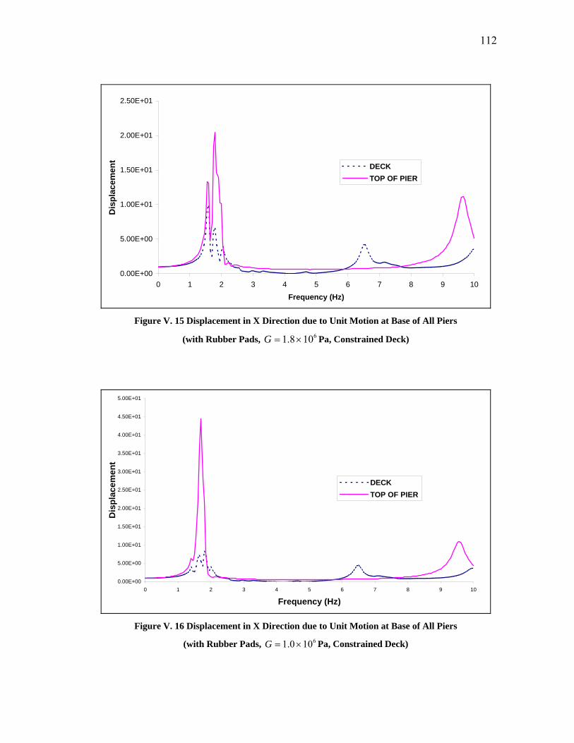
112
0.00E+00
5.00E+00
1.00E+01
1.50E+01
2.00E+01
2.50E+01
0 1 2 3 4 5 6 7 8 9 10
Frequency (Hz)
Dis
plac
emen
t
DECKTOP OF PIER
Figure V. 15 Displacement in X Direction due to Unit Motion at Base of All Piers
(with Rubber Pads, 6108.1 ×=G Pa, Constrained Deck)
0.00E+00
5.00E+00
1.00E+01
1.50E+01
2.00E+01
2.50E+01
3.00E+01
3.50E+01
4.00E+01
4.50E+01
5.00E+01
0 1 2 3 4 5 6 7 8 9 10
Frequency (Hz)
Dis
plac
emen
t
DECKTOP OF PIER
Figure V. 16 Displacement in X Direction due to Unit Motion at Base of All Piers
(with Rubber Pads, 6100.1 ×=G Pa, Constrained Deck)

113
5.3.2 Transverse Direction (Y direction)
In the transverse direction, without rubber pads, the first three significant peaks would be
at 1.85Hz, 2.70Hz and 4.90Hz, respectively, as shown in Figure V.17, which illustrates
the transfer function at the top of pier 4 due to a unit harmonic motion in the transverse
direction at the bottoms of all the piers. The first two significant peaks are in relatively
good agreement with those of the second and third mode in D. Romo’s model for the
same case (1.79Hz and 2.67Hz).
0.00E+00
5.00E+00
1.00E+01
1.50E+01
2.00E+01
2.50E+01
3.00E+01
0 1 2 3 4 5 6 7 8 9 10Frequency (Hz)
Dis
plac
emen
t
Figure V. 17 Displacement in Y Direction at Top of Pier 4 due to Unit Motion at Base of All Piers
(without Rubber Pads)
Figure V.18 shows the transfer functions for a free deck and a shear modulus of the
rubber pads of 6.0Mpa. It can be seen that the motion of the deck has a significant peak
at 0.90 Hz and two small peaks at 1.15Hz and 5.7Hz, while the motion of the top of the
pier has a significant peak at 5.7Hz and a small one at 0.9Hz. As the shear modulus
reduces to 1.8Mpa and 1.0Mpa as shown in Figure V.18 and Figure V.19, the significant

114
peak for the deck decreases to 0.55Hz and 0.45Hz, respectively; while that of the top of
the deck takes place at 5.3Hz and 5.25Hz, respectively. The peak at 0.90Hz frequency
agrees with the results of D. Romo and the V.M. Daza (0.93Hz and 0.96Hz) while the
1.15Hz frequency agrees with the experimental data (1.17Hz and 1.07Hz).
0.00E+00
5.00E+00
1.00E+01
1.50E+01
2.00E+01
2.50E+01
0 1 2 3 4 5 6 7 8 9 10
Frequency(Hz)
Dis
plac
emen
t
DECKTOP OF PIER
Figure V. 18 Displacement in Y Direction due to Unit Motion at Base of All Piers
(with Rubber Pads, 6100.6 ×=G Pa, Free Deck)

115
0.00E+00
5.00E+00
1.00E+01
1.50E+01
2.00E+01
2.50E+01
0 1 2 3 4 5 6 7 8 9 10Frequency (Hz)
Dis
plac
emen
t
DECKTOP OF PIER
Figure V. 19 Displacement in Y Direction due to Unit Motion at Base of All Piers
(with Rubber Pads, 6108.1 ×=G Pa, Free Deck)
0.00E+00
5.00E+00
1.00E+01
1.50E+01
2.00E+01
2.50E+01
3.00E+01
0 1 2 3 4 5 6 7 8 9 10
Frequency (Hz)
Dis
plac
emen
t
DECKTOP OF PIER
Figure V. 20 Displacement in Y Direction due to Unit Motion at Base of All Piers
(with Rubber Pads, 6100.1 ×=G Pa, Free Deck)
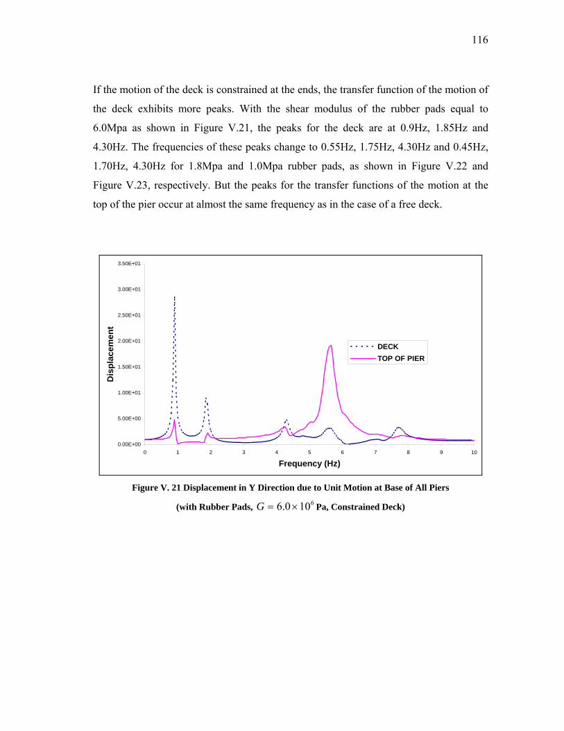
116
If the motion of the deck is constrained at the ends, the transfer function of the motion of
the deck exhibits more peaks. With the shear modulus of the rubber pads equal to
6.0Mpa as shown in Figure V.21, the peaks for the deck are at 0.9Hz, 1.85Hz and
4.30Hz. The frequencies of these peaks change to 0.55Hz, 1.75Hz, 4.30Hz and 0.45Hz,
1.70Hz, 4.30Hz for 1.8Mpa and 1.0Mpa rubber pads, as shown in Figure V.22 and
Figure V.23, respectively. But the peaks for the transfer functions of the motion at the
top of the pier occur at almost the same frequency as in the case of a free deck.
0.00E+00
5.00E+00
1.00E+01
1.50E+01
2.00E+01
2.50E+01
3.00E+01
3.50E+01
0 1 2 3 4 5 6 7 8 9 10
Frequency (Hz)
Dis
plac
emen
t
DECKTOP OF PIER
Figure V. 21 Displacement in Y Direction due to Unit Motion at Base of All Piers
(with Rubber Pads, 6100.6 ×=G Pa, Constrained Deck)

117
0.00E+00
5.00E+00
1.00E+01
1.50E+01
2.00E+01
2.50E+01
3.00E+01
3.50E+01
0 1 2 3 4 5 6 7 8 9 10
Frequency (Hz)
Dis
plac
emen
t
DECKTOP OF PIER
Figure V. 22 Displacement in Y Direction due to Unit Motion at Base of All Piers
(with Rubber Pads, 6108.1 ×=G Pa, Constrained Deck)
0.00E+00
5.00E+00
1.00E+01
1.50E+01
2.00E+01
2.50E+01
0 1 2 3 4 5 6 7 8 9 10
Frequency (Hz)
Dis
plac
emen
t
DECKTOP OF PIER
Figure V. 23 Displacement in Y Direction due to Unit Motion at Base of All Piers
(with Rubber Pads, 6100.1 ×=G Pa, Constrained Deck)

118
5.3.3 Vertical Direction (Z direction)
The frequency response in the vertical direction depends on the Young’s modulus of the
rubber pads rather than their shear modulus. Since the rubber pads are made of
alternating layers of rubber and steel, they are not isotropic. Some studies indicated that
the rubber pads used in the Marga-Marga bridge have a Young’s modulus between
1.35Gpa and 2.40Gpa.
0.00E+00
2.00E-01
4.00E-01
6.00E-01
8.00E-01
1.00E+00
1.20E+00
1.40E+00
1.60E+00
1.80E+00
2.00E+00
0 1 2 3 4 5 6 7 8 9 10Frequency (Hz)
Dis
plac
emen
t
Figure V. 24 Displacement in Z Direction at Top of Pier 4 due to Unit Motion at Base of All Piers
(without Rubber Pads)
Without rubber pads, the transfer function of the displacement at the top of pier 4 due to
a unit vertical harmonic motion at the bottoms of all piers is shown in Figure V.24. It can
be seen that the first significant peak occurs around 3.55Hz. This value agrees well with
the first natural frequency of 3.36Hz reported by D. Romo for the same case.

119
With the introduction of rubber pads with a Young’s modulus of 6.0Gpa or 1.8Gpa, the
first significant peak still happens around 3.55Hz although there are some small
fluctuations between 2.20Hz and 2.80Hz, as shown in Figures V.25 and V.26. A peak at
2.20Hz would be consistent with the natural frequency of 2.18Hz reported by D. Romo
and frequencies of 1.88Hz and 2.10Hz obtained by V.M. Daza. The largest amplification
occurs however at 3.55Hz, a frequency not reported in their studies. It can be concluded
that the frequency at which the significant peak happens is almost independent of the
introduction of the rubber pads or their Young’s modulus. But as the Young’s modulus
decreases, the amplitude of the peak corresponding to the displacement at the deck
increases.
0.00E+00
5.00E-01
1.00E+00
1.50E+00
2.00E+00
2.50E+00
3.00E+00
3.50E+00
0 1 2 3 4 5 6 7 8 9 10
Frequency (Hz)
Dis
plac
emen
t
DECKTOP OF PIER
Figure V. 25 Displacement in Z Direction due to Unit Motion at Base of All Piers
(with Rubber Pads, 9108.1 ×=E Pa, Free Deck)

120
0.00E+00
5.00E-01
1.00E+00
1.50E+00
2.00E+00
2.50E+00
3.00E+00
0 1 2 3 4 5 6 7 8 9 10
Frequency(Hz)
Dis
plac
emen
t
DECKTOP OF PIER
Figure V. 26 Displacement in Z Direction due to Unit Motion at Base of All Piers
(with Rubber Pads, 9100.6 ×=E Pa, Free Deck)
5.4 Conclusions
1. When comparing the results of the present study to those reported by previous
researchers at the University of Chile one should take into account that, in
addition to the difference in the structural models, the results presented here are
transfer functions reflecting the natural frequencies and also the participation
factors of various modes, while the previous studies provided the natural
frequencies of all the modes. Some of these modes might have a very small
participation factor, not get excited by the assumed base motions, and not show
as a result in the transfer functions;
2. In the longitudinal direction, this study yields results very similar to those of D.
Romo, except that if the deck is free and the rubber pads have a 5% shear

121
deformation, the first natural frequency from this work (0.45Hz) is much lower
than that from the model of D. Romo (0.65Hz). This study has 0.65Hz as the first
longitudinal natural frequency when the shear modulus of the rubber pads is
6.0Mpa, which corresponds to a shear deformation of only 0.23%;
3. In the transverse direction, this research gives smaller natural frequencies than
the model of D. Romo. But when the shear modulus of the rubber pads is 6.0Mpa
(0.23% shear deformation), the results from this research are again very similar
to the model of D.Romo with 5% shear deformation;
4. For the cases with rubber pads, the transfer function at the top of the pier
assuming a constrained deck are almost the same as for a free deck. This implies
that the constraints on the ends of the deck will not change the motion at the top
of the pier very much. Actually, the two ends of the deck are neither entirely
fixed in the two horizontal directions, nor absolutely free. The abutments will
restrain the motion of the deck but the deck can still slide over the abutments;
5. The constraints on the two ends of the deck will not change the first transverse
natural frequency, in which mode the deck slides over the relatively soft rubber
pads. This is because the deck is very long so the bending strain energy in the
first mode (half harmonic shape) is very small if the two ends of the deck are
fixed transversely compared with the strain energy associated with the shear
deformation of the rubber pads. For smaller values of the shear modulus of the
rubber pads, restraining the motion of the deck at the ends will have a larger
effect on the first natural frequency.

122
CHAPTER VI
EFFECT OF SOIL STRUCTURE INTERACTION
The transfer functions in the previous chapter were obtained assuming rigid foundations.
This assumption may not be very realistic in some cases, especially for soft soils. To
account for the finite stiffness of the foundations, soil structure interaction (SSI) analyses
are conducted in this chapter.
The numbering of the structure’s model is the same as shown in Figures V.6 & V.7. The
nodes on the south and north abutment (nodes 22 and 30 in Figure V.6 or nodes 1 and 30
in Figure V.7) are still fixed for all 6 degrees of freedom, while the nodes under each
pier (nodes 1, 4, 7, 10, 13, 16 and 19 in Figure V.6 or nodes 2, 6, 10, 14, 18, 22 and 26 in
Figure V.7) are fixed against rotation around the Z axis but supported by springs with
finite stiffness for the other 5 degrees of freedom to model the finite stiffness of the
foundation. The properties and stiffness of the pile foundations (at the pile heads) of the
Marga-Marga bridge were obtained in Chapter IV. The properties of the deck, piers and
rubber pads are the same as those used in Chapter V.
The computer software described in previous chapters was applied again to the Marga-
Marga bridge, but including the stiffness of the pile foundations, to compare the results
with those without SSI and, to evaluate its potential importance.
6.1 Assumptions
Two important assumptions were made to calculate the transfer functions of the system
in this chapter. First, each pile cap has 6 degrees of freedom (DoFs), and the application
of a unit force in any direction may cause displacements in the others. This is known as
the coupling between the different DoFs, such as the coupling between the horizontal

123
and the rocking stiffness. In this study, the coupling terms were neglected because they
are relatively unimportant. (The coupling term between the horizontal and the rocking
stiffness is very small compared with the horizontal or rocking stiffness themselves.)
The stiffness matrix of a pile foundation used here is a diagonal matrix, and all the non-
diagonal terms are zero, as shown in equation VI.1.
[ ]
⎥⎥⎥⎥⎥⎥⎥
⎦
⎤
⎢⎢⎢⎢⎢⎢⎢
⎣
⎡
=
)(000000)(000000)(000000)(000000)(000000)(
)(
ωω
ωω
ωω
ω
z
y
x
z
y
x
Pile
TR
RS
SS
K …………....….…...(VI.1)
in which xS , yS , zS , xR and yR denote the horizontal dynamic stiffness in the X and
Y directions, the vertical stiffness in the Z direction, and the rocking stiffness around
the X axis and around the Y axis, respectively; zT represents the torsional stiffness
around the Z axis, assumed to be infinite in this case.
The other simplifying assumption is that in calculating the dynamic stiffness of one pile
group, the existence of the other pile groups can be neglected, because the distance
between two pile groups (about 50 meters for the Marga-Marga bridge) is much larger
than the horizontal dimension of the pile groups themselves (5.5 meters in the X
direction).
6.2 Loads
In the previous chapter, for the structure with rigid foundations, a unit harmonic
displacement was applied at the bottom of each pier. In this chapter, the bottoms of the
piers are not fixed any more due to the finite stiffness of the pile foundations. The unit
displacement would be applied at the bottom of the equivalent springs representing the
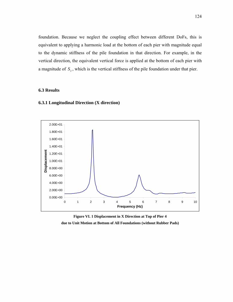
124
foundation. Because we neglect the coupling effect between different DoFs, this is
equivalent to applying a harmonic load at the bottom of each pier with magnitude equal
to the dynamic stiffness of the pile foundation in that direction. For example, in the
vertical direction, the equivalent vertical force is applied at the bottom of each pier with
a magnitude of zS , which is the vertical stiffness of the pile foundation under that pier.
6.3 Results
6.3.1 Longitudinal Direction (X direction)
0.00E+00
2.00E+00
4.00E+00
6.00E+00
8.00E+00
1.00E+01
1.20E+01
1.40E+01
1.60E+01
1.80E+01
2.00E+01
0 1 2 3 4 5 6 7 8 9 10Frequency (Hz)
Dis
plac
emen
t
Figure VI. 1 Displacement in X Direction at Top of Pier 4
due to Unit Motion at Bottom of All Foundations (without Rubber Pads)

125
Table VI. 1 Effect of SSI on Peaks of Transfer Function in Longitudinal Direction (Hz) Without SSI With SSI
Shear Modulus of Rubber Pads First
Peak
Second
Peak
Third
Peak
First
Peak
Second
Peak
Third
Peak
No Rubber Pads 2.15 5.85 2.13 5.75
6.0Mpa(free deck) 0.65 2.75 0.60 2.65
1.8Mpa(free deck) 0.45 1.95 0.40 1.80
1.0Mpa(free deck) 0.35 1.70 0.35 1.60
6.0Mpa(constrained deck) 1.70 2.50 2.85 1.70 2.45 2.60
1.8Mpa(constrained deck) Between 1.5 and 2.0 Between 1.5 and 2.0
1.0Mpa(constrained deck) Between 1.5 and 2.0 Between 1.5 and 2.0
Due to the finite stiffness of the foundations, the natural frequencies of the soil structure
system are expected to be smaller than those of the structure on rigid foundations.
Figure VI.1 shows the transfer function at the top of pier 4 in the X direction without
rubber pads. It can be seen that the two significant peaks are at 2.13Hz and 5.75Hz,
which are only slightly smaller than those of the case without SSI (2.15Hz and 5.85Hz).
Figures VI.2 to VI.9 show the transfer functions at the top of pier 4 and the deck for the
case with rubber pads and SSI. The change in the frequencies of the significant peaks
due to the consideration of the SSI is summarized in Table VI.1.
It can be concluded that the effect of SSI is very small in the longitudinal direction in
relation to the first few natural frequencies of the structure because the positions of the
peaks change very little. Even some small peaks appear at the same frequencies as in the
case without SSI. (For example, there is also a small peak for the motion of the deck
around 6.6Hz for the constrained deck.)
The SSI effects are more pronounced for high frequencies. Whether the deck is
constrained or not, the motion at the top of the pier has a large peak around 10.0Hz

126
without SSI. This peak is greatly de-amplified and shifted to a value between 8Hz to
9Hz (shown in Figures VI.2 to VI.9) when the SSI effect is included. Figures VI.10 &
VI.11 show the transfer functions for the motion at the base of pier 4 in the longitudinal
direction when the same harmonic motion is applied at the base of all foundations. It can
be seen that the motion is a function of the frequency, rather than a constant of 1 as
would be obtained without SSI effect. The base motion of the pier can be amplified up to
30% or de-amplified up to 40%. Between 0.0 and 3.0 Hz the SSI effect results in small
changes in the frequencies of the peaks resulting in a relatively sharp peak followed by a
valley. The motion increases smoothly between 3.0 and 7.5 Hz. Between approximately
8.0 and 10.0 Hz there is a significant reduction in the amplitude of the motions. This is
the range of frequencies over which the flexibility of the foundations would have the
most significant effect in the longitudinal direction.
0.00E+00
5.00E+00
1.00E+01
1.50E+01
2.00E+01
2.50E+01
3.00E+01
0 1 2 3 4 5 6 7 8 9 10
Frequency(Hz)
Dis
plac
emen
t
DECKTOP OF PIER
Figure VI. 2 Displacement in X Direction due to Unit Motion at Base of All Foundations
(with Rubber Pads, 6100.6 ×=G Pa, Free Deck)

127
0.00E+00
2.00E+00
4.00E+00
6.00E+00
8.00E+00
1.00E+01
1.20E+01
1.40E+01
1.60E+01
1.80E+01
2.00E+01
0 1 2 3 4 5 6 7 8 9 10
Frequency(Hz)
Dis
plac
emen
t
DECKTOP OF PIER
Figure VI. 3 Displacement in X Direction due to Unit Motion at Base of Foundation under Pier 4
(with Rubber Pads, 6100.6 ×=G Pa, Free Deck)
0.00E+00
5.00E+00
1.00E+01
1.50E+01
2.00E+01
2.50E+01
3.00E+01
0 1 2 3 4 5 6 7 8 9 10
Frequency(Hz)
Dis
plac
emen
t
DECKTOP OF PIER
Figure VI. 4 Displacement in X Direction due to Unit Motion at Base of All Foundations
(with Rubber Pads, 6108.1 ×=G Pa, Free Deck)

128
0.00E+00
5.00E+00
1.00E+01
1.50E+01
2.00E+01
2.50E+01
3.00E+01
3.50E+01
0 1 2 3 4 5 6 7 8 9 10
Frequency(Hz)
Dis
plac
emen
t DECKTOP OF PIER
Figure VI. 5 Displacement in X Direction due to Unit Motion at Base of All Foundations
(with Rubber Pads, 6100.1 ×=G Pa, Free Deck)
0.00E+00
5.00E+00
1.00E+01
1.50E+01
2.00E+01
2.50E+01
3.00E+01
0 1 2 3 4 5 6 7 8 9 10
Frequency(Hz)
Dis
plac
emen
t
DECKTOP OF PIER
Figure VI. 6 Displacement in X Direction due to Unit Motion at Base of All Foundations
(with Rubber Pads, 6100.6 ×=G Pa, Constrained Deck)

129
0.00E+00
2.00E+00
4.00E+00
6.00E+00
8.00E+00
1.00E+01
1.20E+01
1.40E+01
1.60E+01
1.80E+01
2.00E+01
0 1 2 3 4 5 6 7 8 9 10
Frequency(Hz)
Dis
plac
emen
t DECKTOP OF PIER
Figure VI. 7 Displacement in X Direction due to Unit Motion at Base of Foundation under Pier 4
(with Rubber Pads, 6100.6 ×=G Pa, Constrained Deck)
0.00E+00
5.00E+00
1.00E+01
1.50E+01
2.00E+01
2.50E+01
3.00E+01
3.50E+01
4.00E+01
0 1 2 3 4 5 6 7 8 9 10
Frequency(Hz)
Dis
plac
emen
t
DECKTOP OF PIER
Figure VI. 8 Displacement in X Direction due to Unit Motion at Base of All Foundations
(with Rubber Pads, 6108.1 ×=G Pa, Constrained Deck)

130
0.00E+00
5.00E+00
1.00E+01
1.50E+01
2.00E+01
2.50E+01
3.00E+01
3.50E+01
4.00E+01
4.50E+01
5.00E+01
0 1 2 3 4 5 6 7 8 9 10
Frequency(Hz)
Dis
plac
emen
t
DECKTOP OF PIER
Figure VI. 9 Displacement in X Direction due to Unit Motion at Base of All Foundations
(with Rubber Pads, 6100.1 ×=G Pa, Constrained Deck)
0.00E+00
2.00E-01
4.00E-01
6.00E-01
8.00E-01
1.00E+00
1.20E+00
1.40E+00
0 1 2 3 4 5 6 7 8 9 10
Frequency(Hz)
Dis
plac
emen
t
G=1Mpa
G=1.8Mpa
G=6Mpa
Figure VI. 10 Motion of the Base of Pier 4 When All Foundations Are Excited in the X Direction
(Free Deck)

131
0.00E+00
2.00E-01
4.00E-01
6.00E-01
8.00E-01
1.00E+00
1.20E+00
1.40E+00
0 1 2 3 4 5 6 7 8 9 10Frequency(Hz)
Dis
plac
emen
t
G=1Mpa
G=1.8Mpa
G=6Mpa
Figure VI. 11 Motion of the Base of Pier 4 When All Foundations Are Excited in the X Direction
(Constrained Deck)
6.3.2 Transverse Direction (Y direction)
The effects of the SSI on the frequencies of the peaks of the transfer functions in the
transverse direction are summarized in Table VI.2 and illustrated in Figures VI.12 to
VI.18. It is somewhat larger than in the longitudinal direction. The reason is that the
bending stiffness of the 7 piers is larger transversely than longitudinally.
For the structure without rubber pads, the effect is very clear. The first three significant
peaks change from 1.85Hz, 2.70Hz and 4.90Hz to 1.45Hz, 2.45Hz and 4.75Hz. With the
introduction of the rubber pads, the effect of soil structure interaction is less pronounced.
Table VI.2 shows that the change in the frequency of the peaks for the isolated system is
very small for the first peak (about 10% with a free deck and less when the deck is
restrained). It is more significant on the motion and peaks of the pier than those of the
deck (comparing the fourth peak without SSI and the third peak with SSI). Both for the

132
0.00E+00
2.00E+00
4.00E+00
6.00E+00
8.00E+00
1.00E+01
1.20E+01
1.40E+01
1.60E+01
1.80E+01
0 1 2 3 4 5 6 7 8 9 10Frequency (Hz)
Dis
plac
emen
t
Figure VI. 12 Displacement in Y Direction at Top of Pier 4
due to Unit Motion at Bottom of All Foundations (without Rubber Pads)
Table VI. 2 Effect of SSI on Peaks of Transfer Function in Transverse Direction (Hz)
Without SSI With SSI Shear Modulus of
Rubber Pads 1st
Peak
2nd
Peak
3rd Peak
(Deck)
4th Peak
(Pier)
1st
Peak
2nd
Peak
3rd Peak
(Pier)
4th Peak
(Deck)
No Rubber Pads 1.85 2.70 4.90 1.45 2.45 4.75
6.0Mpa(free deck) 0.90 5.70 0.85 1.12 4.05
1.8Mpa(free deck) 0.55 5.30 0.50 3.70
1.0Mpa(free deck) 0.45 5.25 0.40 3.60
6.0Mpa(constrained deck) 0.90 1.85 4.30 5.70 0.85 1.85 4.05 4.45
1.8Mpa(constrained deck) 0.55 1.75 4.30 5.30 0.55 1.75 3.70 4.30
1.0Mpa(constrained deck) 0.45 1.70 4.30 5.25 0.45 1.70 3.60 4.27

133
pier and the deck the main interaction effects in the transverse direction occur in the
frequency range between 3 and 6Hz, whereas in the longitudinal direction the range was
8 to 11Hz.
From Figures VI.19 & VI.20, it can also be seen that the SSI effect is more prominent in
the transverse direction than in the longitudinal direction, because the base motion of
pier 4 is amplified or de-amplified more in the transverse than in the longitudinal
direction.
0.00E+00
5.00E+00
1.00E+01
1.50E+01
2.00E+01
2.50E+01
0 1 2 3 4 5 6 7 8 9 10
Frequency(Hz)
Dis
plac
emen
t
DECKTOP OF PIER
Figure VI. 13 Displacement in Y Direction due to Unit Motion at Base of All Foundations
(with Rubber Pads, 6100.6 ×=G Pa, Free Deck)

134
0.00E+00
2.00E+00
4.00E+00
6.00E+00
8.00E+00
1.00E+01
1.20E+01
1.40E+01
1.60E+01
1.80E+01
0 1 2 3 4 5 6 7 8 9 10
Frequency(Hz)
Dis
plac
emen
t
DECKTOP OF PIER
Figure VI. 14 Displacement in Y Direction due to Unit Motion at Base of All Foundations
(with Rubber Pads, 6108.1 ×=G Pa, Free Deck)
0.00E+00
1.00E+01
2.00E+01
3.00E+01
4.00E+01
5.00E+01
6.00E+01
7.00E+01
0 1 2 3 4 5 6 7 8 9 10
Frequency(Hz)
Dis
plac
emen
t
DECKTOP OF PIER
Figure VI. 15 Displacement in Y Direction due to Unit Motion at Base of All Foundations
(with Rubber Pads, 6100.1 ×=G Pa, Free Deck)

135
0.00E+00
5.00E+00
1.00E+01
1.50E+01
2.00E+01
2.50E+01
3.00E+01
3.50E+01
4.00E+01
0 1 2 3 4 5 6 7 8 9 10
Frequency(Hz)
Dis
plac
emen
t
DECKTOP OF PIER
Figure VI. 16 Displacement in Y Direction due to Unit Motion at Base of All Foundations
(with Rubber Pads, 6100.6 ×=G Pa, Constrained Deck)
0.00E+00
5.00E+00
1.00E+01
1.50E+01
2.00E+01
2.50E+01
3.00E+01
3.50E+01
4.00E+01
4.50E+01
0 1 2 3 4 5 6 7 8 9 10
Frequency(Hz)
Dis
plac
emen
t
DECKTOP OF PIER
Figure VI. 17 Displacement in Y Direction due to Unit Motion at Base of All Foundations
(with Rubber Pads, 6108.1 ×=G Pa, Constrained Deck)

136
0.00E+00
2.00E+00
4.00E+00
6.00E+00
8.00E+00
1.00E+01
1.20E+01
1.40E+01
1.60E+01
1.80E+01
0 1 2 3 4 5 6 7 8 9 10
Frequency(Hz)
Dis
plac
emen
t
DECKTOP OF PIER
Figure VI. 18 Displacement in Y Direction due to Unit Motion at Base of All Foundations
(with Rubber Pads, 6100.1 ×=G Pa, Constrained Deck)
0.00E+00
2.00E-01
4.00E-01
6.00E-01
8.00E-01
1.00E+00
1.20E+00
1.40E+00
1.60E+00
0 1 2 3 4 5 6 7 8 9 10Frequency(Hz)
Dis
plac
emen
t
G=1Mpa
G=1.8Mpa
G=6Mpa
Figure VI. 19 Motion of the Base of Pier 4 When All Foundations Are Excited in the Y Direction
(Free Deck)

137
0.00E+00
2.00E-01
4.00E-01
6.00E-01
8.00E-01
1.00E+00
1.20E+00
1.40E+00
1.60E+00
0 1 2 3 4 5 6 7 8 9 10Frequency(Hz)
Dis
plac
emen
t
G=1Mpa
G=1.8Mpa
G=6Mpa
Figure VI. 20 Motion of the Base of Pier 4 When All Foundations Are Excited in the Y Direction
(Constrained Deck)
6.3.3 Vertical Direction (Z direction)
As shown in Figures VI.21 to VI.23, the effect of SSI in the vertical direction is still very
small. The position of the only significant peak decreases from 3.55Hz to 3.45Hz due to
the effect of SSI, and the introduction of the rubber pads has a negligible effect on it.
The major effect of SSI is to increase the amplification ratio, an effect very similar to
that of the rubber pads. For the case without rubber pads the ratio increases from 1.8 to
2.4 due to SSI. As the Young’s modulus of the rubber pads decreases, the effect of SSI
becomes smaller.

138
0.00E+00
5.00E-01
1.00E+00
1.50E+00
2.00E+00
2.50E+00
0 1 2 3 4 5 6 7 8 9 10Frequency (Hz)
Dis
plac
emen
t
Figure VI. 21 Displacement in Z Direction at Top of Pier 4
due to Unit Motion at Bottom of All Foundations (without Rubber Pads)
0.00E+00
5.00E-01
1.00E+00
1.50E+00
2.00E+00
2.50E+00
3.00E+00
3.50E+00
0 1 2 3 4 5 6 7 8 9 10
Frequency(Hz)
Dis
plac
emen
t
DECKTOP OF PIER
Figure VI. 22 Displacement in Z Direction due to Unit Motion at Base of All Foundations
(with Rubber Pads, 9100.6 ×=E Pa, Free Deck)

139
0.00E+00
5.00E-01
1.00E+00
1.50E+00
2.00E+00
2.50E+00
3.00E+00
3.50E+00
0 1 2 3 4 5 6 7 8 9 10
Frequency(Hz)
Dis
plac
emen
t
DECKTOP OF PIER
Figure VI. 23 Displacement in Z Direction due to Unit Motion at Base of All Foundations
(with Rubber Pads, 9108.1 ×=E Pa, Free Deck)
6.3.4 Effect of Soil Properties
To study further the potential SSI effects, the soil properties were reduced over the top
12 meters to simulate some nonlinear soil behavior. The foundation stiffness terms were
calculated again for this case. The assumed properties and the calculated foundation
stiffness were shown in Tables IV.7 ~ IV.10 and Figures IV.23 ~ IV.33. The new
foundation stiffness terms with reduced soil shear modulus were discussed in §4.4.
Tables VI.3 & VI.4 show the change of the frequencies of the peaks of the transfer
functions due to the new soil profile. The decrease in the frequencies for the structure on
the new, softer, soils is larger than that on the original soils, as could be expected but it is
still very small in the longitudinal direction and only a little larger in the transverse
direction.

140
Table VI. 3 Effect of SSI on Peaks of Transfer Function in Longitudinal Direction (Hz)
(with New Soil Properties)
Without SSI With SSI
(New Soil Properties) Shear Modulus of Rubber Pads 1st
Peak
2nd
Peak
3rd
Peak
1st
Peak
2nd
Peak
3rd
Peak
No Rubber Pads 2.15 5.85 2.10 5.62
6.0Mpa(free deck) 0.65 2.75 0.60 2.60
1.8Mpa(free deck) 0.45 1.95 0.40 1.75
1.0Mpa(free deck) 0.35 1.70 0.35 1.55
6.0Mpa(constrained deck) 1.70 2.50 2.85 1.70 2.40 2.60
1.8Mpa(constrained deck) Between 1.5 and 2.0 Between 1.5 and 2.0
1.0Mpa(constrained deck) Between 1.5 and 2.0 Between 1.5 and 2.0
Table VI. 4 Effect of SSI on Peaks of Transfer Function in Transverse Direction (Hz) (with New Soil Properties)
Without SSI With SSI
(New Soil Properties) Shear Modulus of Rubber Pads 1st
Peak
2nd
Peak
3rd Peak
(Deck)
4th Peak
(Pier)
1st
Peak
2nd
Peak
3rd Peak
(Pier)
4th Peak
(Deck)
No Rubber Pads 1.85 2.70 4.90 1.30 2.35 4.60
6.0Mpa(free deck) 0.90 5.70 0.80 1.10 3.85
1.8Mpa(free deck) 0.55 5.30 0.50 3.40
1.0Mpa(free deck) 0.45 5.25 0.40 3.35
6.0Mpa(constrained deck) 0.90 1.85 4.30 5.70 0.80 1.80 3.85 4.30
1.8Mpa(constrained deck) 0.55 1.75 4.30 5.30 0.55 1.75 3.40 4.30
1.0Mpa(constrained deck) 0.45 1.70 4.30 5.25 0.45 1.70 3.35 4.27

141
6.4 Conclusions
1) Generally, soil structure interaction (SSI) changes the frequencies of the peaks of
the transfer functions. The effects of SSI on the first natural frequencies are very
small for the conditions of the Marga-Marga bridge. These conclusions had also
been reached by V.M. Daza in his work. They are somewhat larger in the
transverse than in the longitudinal direction;
2) For the structure without rubber pads, the effect of soil structure interaction is
more pronounced. The frequencies of the peaks of the transfer functions decrease
clearly;
3) For the structure with rubber pads, SSI has some small effects on the motion at
the top of the pier, but since the deck has been isolated by rubber pads, the
motions of the deck are affected much less;
4) The main SSI effects are in the range of frequencies between 3.0 and 5.0 Hz in
the transverse direction and above 8.0Hz in the longitudinal direction.

142
CHAPTER VII
CONCLUSIONS AND RECOMMENDATIONS
7.1 General Observations
The studies carried out and described in Chapters V and VI indicate that:
1) The presence of the isolation pads reduces considerably the amplitude of the
longitudinal deck motions with respect to those at top of the pier except at the
first natural frequency of the system, which varies from 0.35Hz to 1.7Hz
depending on the assumed conditions at the ends of the deck (free deck or
constrained deck). At this frequency the motion of the deck seems to be larger
than that of the top of the pier for a free deck (the frequency is that of the deck
vibrating as a free body on top of the rubber pads). For a constrained deck, the
amplitude of the motion of the deck is much smaller than that of the pier for the
smaller values of the assumed shear modulus (as the level of excitation and
therefore the level of deformation of the rubber pads increase). The only other
exception is at around 6.5Hz when the deck is constrained and the same motion
is applied at the base of all the piers.
Comparing the transfer functions for the motion of the deck in Figures VI.2 ~
VI.9 with that for the case without rubber pads (Figure VI.1) one can reach the
same conclusion. The inclusion of the rubber pads will reduce the motions of the
deck over most ranges of frequencies (except for the fundamental frequency).
If the energy of the earthquake is not around the fundamental frequency of the
deck (Chilean earthquakes tend to have predominant frequencies of 3.0Hz to
4.0Hz) the effect of the rubber pads on the seismic motions of the deck in the
longitudinal direction will be very beneficial. Comparing on the other hand the

143
transfer functions of the motion on the top of pier 4 with and without rubber pads
(same figures) it can be seen that the main effect is in the change in the natural
frequencies but there is no longer a reduction over most of the frequency range:
the amplitudes decrease at the frequencies of the structure without rubber pads
and increase instead at the frequencies (more than one) of the structure with
rubber pads;
2) The effect of the rubber pads on the motion of the deck in the transverse direction
is less pronounced than in the longitudinal direction. While there are important
reductions in amplitude with respect to the top of the pier or with respect to the
deck without rubber pads, there are now several frequency ranges over which the
motion of the deck may be larger than that of the pier (several peaks associated
with the motion of the deck);
3) Comparing the motion at the top of the pier without rubber pads with that with
rubber pads, one can conclude that the presence of the rubber pads increases the
amplitude of the transfer functions around the first vertical natural frequency
(about 3.3Hz for the Marga-Marga bridge). Over the other frequency ranges, the
value of the transfer functions is almost 1. Around the first vertical natural
frequency, the amplitude of the motion at the deck with rubber pads is always
larger than that at the top of the pier.
7.2 Data from a Real Earthquake
Figures VII.1, VII.2 and VII.3 show the Power spectra (square of the amplitude Fourier
spectra of the motions) recorded on the Marga-Marga bridge in the longitudinal,
transverse and vertical directions under an earthquake that occurred on July 24, 2001. In
these three figures, the motion at the free field (on rock at the left of the left abutment) is
shown at the upper-left corner, the motion at the bottom of pier 4 at the upper-right

144
corner, the motion at the top of pier 4 at the lower-left corner, and the motion on top of
the deck at the lower-right corner.
These experimental data show:
1) In the longitudinal direction:
a) A considerable reduction in the motion above 3.0Hz at the three locations
(compared to the free field);
b) A significant peak at about 1.5Hz in the base motion of the pier, which is
considerably reduced on top of the pier and on the deck (square of the
amplitude is 8105.1 × at the base, 7100.2 × at the top of the pier and 6100.6 × on the deck. (a reduction in amplitude by factors of
74.25.7 = at the top of the pier and 0.525 = on the deck);
c) A significant amplification at about 2.7Hz on top of the pier, which is not
present on the deck. (amplification ratio of the amplitude is about
2.3)104/()104( 78 ≈×× from the base to the top of the pier). The
amplitude at the base of the pier at this frequency was slightly smaller
than in the free field;
The first natural frequency in shear of the soil deposit itself is about 1.4Hz from the
analysis in Chapter IV, which explains the peak at about 1.5Hz in the base motion of the
pier. As for the amplification at 2.7Hz, one can find from Figures VI.2 or VI.3 that this
is a natural frequency of the structure and the motion at the top of pier 4 is amplified
very much while the motion of the deck is not. The analysis conducted cannot explain,
on the other hand, the large reductions in motion above 3Hz.

145
Figure VII. 1 FFT of Recorded Longitudinal (X) Motion of Marga-Marga Bridge
during the Earthquake of July 24, 2001
Figure VII. 2 FFT of Recorded Transverse (Y) Motion of Marga-Marga Bridge
during the Earthquake of July 24, 2001

146
2) In the transverse direction,
a) A considerable reduction in the motion above 3.5Hz (especially around
4.0Hz) at the base of the pier and on the deck (compared to the free field).
On the top of the pier the amplitude of motion around 4Hz is similar to
that in the free field;
b) A peak at about 1.3Hz at the base of the pier with an amplitude squared
of 7105.7 × . It is only 7100.4 × at the top of the pier and 7100.2 × on the
deck, a reduction in amplitude by factors of 7.5 / 4.0 1.37≈ at the top of
the pier and 7.5/ 2.5 1.73≈ on the deck;
c) A number of small peaks around 1.0Hz and a more significant peak at
1.5Hz on the deck motions with an amplitude squared of 8105.1 × . This
peak is not present on the motion on top of the pier;
d) A peak at the base and on top of the pier at about 2.8~2.9Hz, with
amplification ratios with respect to the motion at the free field of
35.22/11 ≈ (for the base of the pier) and 32.32/22 ≈ (for the top of
the pier), while the motion is greatly de-amplified on the deck.
The reduction in the motions between 3.5 and 4.5Hz at the base of the pier is
consistent with the reported SSI effect in the transverse direction, but the
reduction above 4.5Hz is not explained by this research. The peak in the base
motion at 1.3Hz is also very close to the shear natural frequency of the soil
deposit calculated in Chapter IV (1.4Hz). For the case with a constrained deck,
Figures VI.16 ~ VI.18 show that the structure has a natural frequency at about
1.7~1.85Hz, where the motion of the deck is greatly amplified (not too far from
the 1.5Hz of the data). From Figure VII.4, which shows the transfer function for
one-dimensional soil amplification, one can find that around 2.8~2.9Hz the

147
amplification ratio of the motion from the outcrop of rock to the free surface is
about 2.2. As one can find from Figures VI.13 ~ VI.20, the amplification ratio at
this frequency from the free surface to the bottom of the pier is about 1.1, to the
top of the pier 2.0 to 2.5 and to the deck 0.25 to 0.35, depending on the shear
modulus of the rubber pads. So the amplification from rock outcrop to the base of
the pier is about 2.4 to 2.7, to the top of the pier about 4.0 and to the deck about
0.55. While these figures do not coincide exactly with those reported from the
experimental data, they follow the same general trend. It should be noticed that
the amplification values will depend on the assumed values of damping.
3) In the vertical direction,
a) These are peaks in the free field motion at 4.0Hz and 4.8Hz. These two
peaks have a very similar amplitude in the motions recorded at the base
and on top of the pier but are amplified on the deck by factors of
0.25.1/6 ≈ (for 4.0Hz) or 9 / 3.5 1.6≈ (for 4.8Hz);
b) A peak at about 2.6Hz at the base, the top of pier and the deck with an
amplitude square of 7105.1 × .
The soil deposit has a dilatational natural frequency of about 2.4Hz as stated in
Chapter IV. The amplitude of the transfer functions at this frequency is nearly
equal at all three locations in the bridge, as shown in Figures VI.22 & VI.23. The
amplification in the motion of the deck at 4Hz and 4.8Hz cannot be explained in
the studies conducted.

148
Figure VII. 3 FFT of Recorded Vertical (Z) Motion of Marga-Marga Bridge
during the Earthquake of July 24, 2001
0
1
2
3
4
5
6
0 1 2 3 4 5 6 7 8 9 10Frequency (Hz)
Tran
sfer
Fun
ctio
n
Figure VII. 4 One-dimensional Horizontal Soil Amplification of the Soil Deposit

149
7.3 Recommendation for Future Studies
1) Nonlinear one-dimensional or two dimensional soil amplification analyses in the
time domain may be needed to give a better estimate of the natural frequencies of
the soil deposit and soil amplification effects;
2) Because the amplification ratio depends strongly on the damping, iterations may
be needed in a linearized analysis of the complete soil-structure-rubber pads
system to get better estimates of the effective hysteretic damping and shear
modulus;
3) The transfer functions are sensitive to the modeling of the rubber pads, which
means that more realistic, nonlinear models of the rubber pads and time domain
nonlinear analyses would improve the prediction of the structural response;
4) The transfer functions can change substantially if the motions at the base of the
various peers are different. In this study it was assumed in most cases that all
supports had the same motion although the program allowed to consider and
combine different motions. On would need however more information on the
potential variations in the motions of the supports.

150
REFERENCES Banerjee, J. R. and William, F. W. (1985). “Exact Bernoulli-Euler dynamic stiffness
matrix for a range of tapered beams.” International Journal for Numerical Methods in Engineering, 21, 2289-2302.
Banerjee, J. R. and William, F. W. (1994a). “An exact dynamic stiffness matrix for coupled extentional-torsional vibration of structural members.” Computers and Structures, 50, 161-166.
Banerjee, J. R. and William, F. W. (1994b). “Coupled bending-torsional dynamic stiffness matrix for an axially loaded Timoshenko beam element.” International Journal of Solids and Structures, 31, 749-762.
Betti, R. (1995). “Dynamic soil-bridge interaction.” Proceedings of Engineering Mechanics, 1, 82-85.
Billings, L. J. (1993). “Finite element modeling of elastomeric seismic isolation bearings.” Ph.D. Dissertation, University of California, Irvine, California.
Carrubba, P., Massimino, M. R. and Maugeri, M. (2003). “Soil nonlinear stiffnesses for SSI involving embedded foundations.” Computational Engineering, 4, 53-62.
Casas, J.R. (1997). “Horizontal bridge-soil interaction assessment by dynamic testing.” Experimental Mechanics, 37(1), 69-77.
Chang C. H. (2002). “Modeling of laminated rubber bearings using an analytical stiffness matrix.” International Journal of Solids and Structures 39, 6055–6078.
Chaudhary, M.T.A., Abe, M. and Fujino, Y. (2001a). “Identification of soil-structure interaction effect in base-isolated bridges from earthquake records.” Soil Dynamics and Earthquake Engineering, 21(8), 713-725.
Chaudhary, M.T.A., Abe, M. and Fujino, Y. (2001b). “Performance evaluation of base-isolated Yama-age bridge with high damping rubber bearings using recorded seismic data.” Engineering Structures, 23(8), 902-910.
Chaudhary, M. T. A., Abe, M. and Fujino, Y. (2002a). “Investigation of atypical seismic response of a base-isolated bridge.” Engineering Structures, 24(7), 945-953.

151
Chaudhary, M.T.A., Abe, M. and Fujino, Y. (2002b). “Role of structural details in altering the expected seismic response of base-isolated bridges.” Mechanical Systems and Signal Processing, 16(2-3), 413-428.
Chaudhary, M. T. A., Abe, M., Fujino, Y. and Yoshida, J. (2000). “System identification of two base-isolated bridges using seismic records.” Journal of Structural Engineering, 126(10), 1187-1195.
Chaudhry, M. S. and Prakash, S. (1998). “Dynamic soil structure interaction for bridge abutments on piles.” Geotechnical Special Publication, 2, 1247-1258.
Chen, Y. H. and Sheu, J. T. (1993). “Axial loaded damped Timoshenko beam on viscoelastic foundation.” International Journal for Numerical Methods in Engineering, 36, 1013-1027.
Chen, Y.-H. and Sheu, J.-T. (1996). “Beam length and dynamic stiffness.” International Computer Methods in Applied Mechanics and Engineering, 129, 311-318.
Consolazio, G. R., Lehr, G. B. and McVay, M. C. (2003). “Dynamic finite element analysis of vessel-pier-soil interaction during barge impact events.” Transportation Research Record, 1849(03-3230), 81-90.
Crouse, C. B. and Price, T. (1993). “Dynamic soil-foundation interaction at the Meloland Road overcrossing.” Engineering in Natural Hazards Mitigation, 355-360.
Crouse, C. B., Hushmand, B. and Martin, G. R. (1987). “Dynamic soil structure interaction of a single-span bridge.” Earthquake Engineering & Structural Dynamics, l5(6), 7ll-729.
Crouse, C.B. and McGuire, J. (2001). “Energy dissipation in soil-structure interaction.” Earthquake Spectra, 17(2), 235-259.
Daza, V. M. (2003). “Interaccion sismica suelo-estructura en el Puente Marga-Marga.” Engineering Thesis, Civil Engineering Department, University of Chile, Santiago, Chile.
Dendrou, B., Werner, S. and Toridis, T. (1984). “Three-dimensional response of a concrete bridge system to traveling seismic waves.” Computers and Structures, 20(1-3), 593-6.

152
Doyle, J. F. (1989a). Wave propagation in structures – an FFT-based spectral analysis methodology, Springer, Verlag, New York.
Doyle, J. F. (1989b). Wave propagation in structures – spectral analysis using fast discrete fourier transform, 2nd. Ed. Springer, Verlag, New York.
Elsabee F. and Morray J. P. (1977). “Dynamic behavior of embedded foundations.” Research Report R77-33, Department of Civil Engineering, MIT, Cambridge, Massachusetts.
Gomez R. (1982). “Rigideces dinamicas de grupos de pilotes.” Tesis de Doctorado Presentada en la Universidad Autonoma de Mexico, Mexico City.
Gopalakrishnan, S. and Doyle, J. F. (1994). “Wave propagation in connected waveguides of varying cross-section.” Journal of Sound and Vibration, 175, 374-363.
Guin, J. and Banerjee, P.K. (1998). “Coupled soil-pile-structure interaction analysis under seismic excitation.” Journal of Structural Engineering, 124(4), 434-444.
Harada, T., Yamashita, N. and Sakanashi, K. (1994). “Theoretical study on fundamental period and damping ratio of bridge pier-foundation system.” Doboku Gakkai Rombun-Hokokushu/Proceedings of the Japan Society of Civil Engineers, 489(1-27), 227-234.
Haringx J. A. (1949). “On highly compressible helical springs and rubber rods, and their application for vibration-free mountings.” III. Philips Research Reports 4, 206–220.
Hino, K. and Tanabe, T. A. (1986). “Nonlinear dynamic response analysis of RC structures on the ground with infinite boundaries.” Transactions of the Japan Concrete Institute, 8, 443-450.
Hutchinson, T.C., Chai, Y.H., Boulanger, R.W. and Idriss, I.M. (2004). “Inelastic seismic response of extended pile-shaft-supported bridge structures.” Earthquake Spectra, 20(4), 1057-1080.
Iwasaki, T., Kawashima, K., Takagi, Y. and Aizawa, K. (1984). “Dynamic soil-structure interaction analysis of Kaihoku Bridge.” Transactions of the Japan Society of Civil Engineers, 14, 67-68.

153
Kaito, K., Abe, M, Fujino, Y and Chaudhary, M. T. A. (1999). “Performance evaluation of a base-isolated bridge using complex modal analysis.” Proceedings of the International Modal Analysis Conference - IMAC, 2, 1749-1755.
Kausel E. (1974). “Forced vibrations of circular foundations on layered media.” Research Report R74-11, Department of Civil Engineering, MIT, Cambridge, Massachusetts.
Kolousěk, V. (1973). Dynamics in engineering structures, Butterworth, London.
Kuribaya, E. and Iida, Y. (1974). “Application of finite element method to soil-foundation interaction analysis.” Radio Engineering and Electronic Physics, 151-158.
Latona, R. W. (1969). “Analysis of building frames for natural frequencies and natural mode shapes.” Inter American Program, Civil Engineering Department, MIT, Cambridge, Massachusetts.
Lee, L. J. and Dasgupta, G. (1984). “Finite element formulation of nonlinear structure-soil interacting system for seismic response analysis.” American Society of Mechanical Engineers, Pressure Vessels and Piping Division (Publication) PVP, 80, 133-146.
Levine, M. B. and Scott, R. F. (1989). “Dynamic response verification of simplified bridge-foundation model.” Journal of Geotechnical Engineering, 115(2), 246-260.
Makris, N., Badoni, D., Delis, E. and Gazetas, G. (1994). “Prediction of observed bridge response with soil-pile-structure interaction.” Journal of Structural Engineering, 120(10), 2992-3011.
Makris, N., Gazetas, G. and Delis, E. (1996). “Dynamic soil-pile-foundation-structure interaction: Records and predictions.” Geotechnique, 46(1), 33-50.
Matsuda, A. (1999). “Three-dimensional finite element analysis of laminated rubber bearings using the selective integration method.” JSME Int. J., Ser. A, 42(1), 40-48.

154
Matsuda, A. (2001). “Evaluation for mechanical properties of laminated rubber bearings using nonlinear finite element analysis with hyperelasticity.” Ph.D. Dissertation, Tsukuba University, Japan.
McGuire, J. W., Cannon, I. B. S., Cofer, W. F. and McLean, D. I. (1998). “Seismic evaluation of pile-founded highway bridge on saturated peat.” Journal of Structural Engineering, 124(1), 71-79.
Mylonakis, G., Nikolaou, A. and Gazetas, G. (1997). “Soil-pile-bridge seismic interaction: kinematic and inertial effects. Part I: soft soil.” Earthquake Engineering & Structural Dynamics, 26(3), 337-359.
Papaleontiou, C. G. (1992). “Dynamic analysis of building structures under combined horizontal and vertical vibrations.” Ph.D. Dissertation, University of Texas, Austin, Texas.
Park, K. S., Jung, H. J. and Lee, I. W. (2002). “A comparative study on seismic performances of base isolation systems for multi-span continuous bridge.” Engineering Structures, 24(8), 1001-1013.
Poulos H. G. (1971). “Behavior of laterally loaded piles II-piles groups.” Journal of the Soil Mechanics and Foundations Division, ASCE, 97(5), 733-751.
Romo, D. (1999). “Analisis de registros sismicos y microambientales en el Puente Marga-Marga.” Engineering Thesis Civil Engineering Department, University of Chile, Santiago, Chile.
Saadeghvaziri, M. A., Yazdani-Motlagh, A. R. and Rashidi, S. (2000). “Effects of soil-structure interaction on longitudinal seismic response of MSSS bridges.” Soil Dynamics and Earthquake Engineering, 20(1-4), 231-242.
Segovia, M. E. (1997). (reference of Daza V. M. (2003) ).
Seki, W., Fukahori, Y., Iseda, Y. and Matsunaga, T. (1987). “A large deformation finite element analysis for multilayer elastomeric bearings.” Transaction of the Meeting of the Rubber Division, 856-870.

155
Shinozuka, M., Chung, H. C., Ichitsubo, M. and Liang, J. (2001). “System identification by video image processing.” Proceedings of SPIE - The International Society for Optical Engineering, 4330, 97-107.
Skinner, R. I., Robinson, H. W. and McVerry, H. C. (1993). An introduction to seismic isolation, Wiley, Chichester, England.
Spyrakos, C. C. (1990). “Assessment of SSI on the longitudinal seismic response of short span bridges.” Engineering Structures, 12(1), 60-66.
Spyrakos, C. C. and Loannidis, G. (2003). “Seismic behavior of a post-tensioned integral bridge including soil-structure interaction (SSI).” Soil Dynamics and Earthquake Engineering, 23(1), 53-63.
Su L., Ahmadi G. and Tadjbakhsh I. G. (1989). “A comparative study of performances of various base isolation systems, part I: shear beam structures.” Earthquake Engineering and Structural Dynamics, 18, 11–32.
Su L., Ahmadi G. and Tadjbakhsh I. G. (1990). “A comparative study of performances of various base isolation systems, Part II: Sensitivity analysis.” Earthquake Engineering and Structural Dynamics, 19, 21–33.
Takayama, M., Tada, H. and Tanaka, R. (1990). “Finite element analysis of laminated rubber bearing used in base-isolation system.” Transaction of the Meeting of the Rubber Division, American Chemical Society, Washington, D.C., 46-62.
Takemiya, H. (1985). “Seismic analysis and design of multi-span continuous high-pier bridges with emphasis on soil-structure interaction.” Transactions of the Japan Society of Civil Engineers, 15, 553-556.
Takemiya, H. and Yamada, Y. (1981). “Layered soil-pile-structure dynamic interaction.” Earthquake Engineering & Structural Dynamics, 9(5), 437-457.
Tan, R.Y. and Cheng, W.M. (1993). “System identification of a non-classically damped linear system” Computers and Structures, 46(1), 67-75.
Tan, R.Y. and Huang, M.C. (2000). “System identification of a bridge with lead-rubber bearings.” Computers and Structures, 74(3), 267-280.

156
Tan, R.Y. and Weng, I.W. (1996). “Identification of dynamic properties of isolated structures.” Engineering Structures, 18(3), 240-246.
Tongaonkar, N. P. and Jangid, R. S. (2003). “Seismic response of isolated bridges with soil-structure interaction.” Dynamics and Earthquake Engineering, 23(4), 287-302.
Wolf, J. P. (1988). Soil-structure-interaction analysis in time domain, Prentice Hall,Englewood Cliffs, New Jersey.
Yamada, Y. and Kawano, K. (1979). “Efficiency of the FEM in the analysis of dynamic soil structure interaction.” Proceedings of the Technical Program, INTERNEPCON: International Electronic Packaging and Production Conferences, 541-551.
Yu, C. P. (1995). “Determination of pile lengths using flexural waves.” Report GR95-3, Geotechnical Engineering Center, Civil Engineering Department, University of Texas, Austin, Texas.
Yu, C. P. (1996). “Effect of vertical earthquake components on bridge response.” Ph.D. Dissertation, University of Texas, Austin, Texas.
Yu, C. P. and Roësset, J. M. (1998). “Dynamic analysis of structures using continuous solutions in frequency domain.” Proceedings of EASEC-6 Conference on Structural Engineering & Construction, Taipei, Taiwan, 2, 1369-1375.
Yu C. P. and Roësset J. M. (2001). “Dynamic stiffness matrix for linear members with distributed mass.” Tamkang Journal of Science and Engineering, 4(4), 253-263.
Zechlin, E. T. and Chai, J. (1998). “Nonlinear dynamic analysis of large diameter pile foundations for the Bay Bridge.” Geotechnical Special Publication, 2, 1223-1234.
Zheng, J. Z. and Takeda, T. (1995). “Effects of soil-structure interaction on seismic response of PC cable-stayed bridge.” Soil Dynamics and Earthquake Engineering, 14(6), 427-43.

157
APPENDIX
MODE SHAPES OF THE BRIDGE IN FIGURE II.5
Figure A.1 The 1st Mode Shape of the Bridge in Figure II.5

158
Figure A.2 The 2nd Mode Shape of the Bridge in Figure II.5
Figure A.3 The 3rd Mode Shape of the Bridge in Figure II.5

159
Figure A.4 The 4th Mode Shape of the Bridge in Figure II.5
Figure A.5 The 5th Mode Shape of the Bridge in Figure II.5

160
Figure A.6 The 6th Mode Shape of the Bridge in Figure II.5
Figure A.7 The 7th Mode Shape of the Bridge in Figure II.5
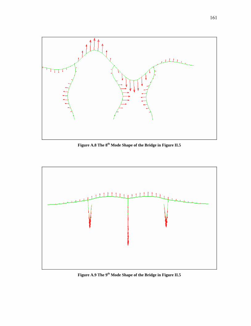
161
Figure A.8 The 8th Mode Shape of the Bridge in Figure II.5
Figure A.9 The 9th Mode Shape of the Bridge in Figure II.5

162
Figure A.10 The 10th Mode Shape of the Bridge in Figure II.5
Figure A.11 The 11th Mode Shape of the Bridge in Figure II.5

163
Figure A.12 The 12th Mode Shape of the Bridge in Figure II.5
Figure A.13 The 13th Mode Shape of the Bridge in Figure II.5

164
Figure A.14 The 14th Mode Shape of the Bridge in Figure II.5
Figure A.15 The 15th Mode Shape of the Bridge in Figure II.5

165
Figure A.16 The 16th Mode Shape of the Bridge in Figure II.5
Figure A.17 The 17th Mode Shape of the Bridge in Figure II.5

166
Figure A.18 The 18th Mode Shape of the Bridge in Figure II.5
Figure A.19 The 19th Mode Shape of the Bridge in Figure II.5
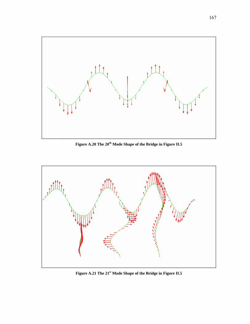
167
Figure A.20 The 20th Mode Shape of the Bridge in Figure II.5
Figure A.21 The 21st Mode Shape of the Bridge in Figure II.5

168
Figure A.22 The 22nd Mode Shape of the Bridge in Figure II.5
Figure A.23 The 23rd Mode Shape of the Bridge in Figure II.5

169
Figure A.24 The 24th Mode Shape of the Bridge in Figure II.5
Figure A.25 The 25th Mode Shape of the Bridge in Figure II.5
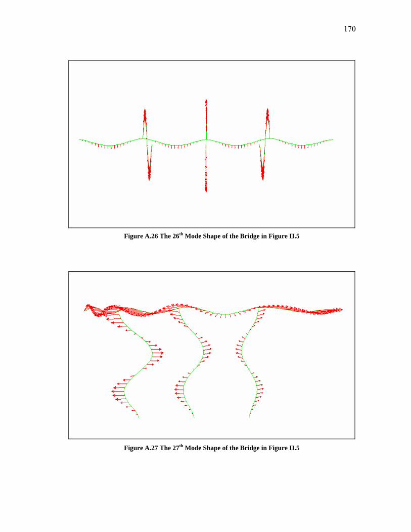
170
Figure A.26 The 26th Mode Shape of the Bridge in Figure II.5
Figure A.27 The 27th Mode Shape of the Bridge in Figure II.5

171
Figure A.28 The 28th Mode Shape of the Bridge in Figure II.5
Figure A.29 The 29th Mode Shape of the Bridge in Figure II.5

172
Figure A.30 The 30th Mode Shape of the Bridge in Figure II.5

173
VITA
Wentao Dai was born in Qingdao, China in August 1976. He received his B.En. and
M.S. degrees in civil engineering from Tongji University, Shanghai, China in July 1999
and March 2002, respectively.
His permanent address and email address are:
4 Le An Er Rd. Apt. 2-302, Qingdao, Shandong 266044, China