Evaluation of Estimation Models using the MinimumInterval of Equivalence

Jose Javier Doladoa,∗, Daniel Rodriguezb, Mark Harmanc,William B. Langdonc, Federica Sarroc

aFacultad de Informatica, UPV/EHU, Univ. of the Basque Country, Spain.bDept. of Computer Science, Universidad de Alcala, 28871, Spain.

cCREST, University College London, WC1E 6BT, UK.

Abstract

This article proposes a new measure to compare soft computing methods for

software estimation. This new measure is based on the concepts of Equivalence

Hypothesis Testing (EHT). Using the ideas of EHT, a dimensionless measure

is defined using the Minimum Interval of Equivalence and a random estima-

tion. The dimensionless nature of the metric allows us to compare methods

independently of the data samples used.

The motivation of the current proposal comes from the biases that other

criteria show when applied to the comparison of software estimation methods.

In this work, the level of error for comparing the equivalence of methods is set

using EHT. Several soft computing methods are compared, including genetic

programming, neural networks, regression and model trees, linear regression

(ordinary and least mean squares) and instance-based methods. The experi-

mental work has been performed on several publicly available datasets (CSC,

China, ISBSG, Maxwell, Desharnais, Atkinson and Telecom1)

Given a dataset and an estimation method we compute the upper point

of Minimum Interval of Equivalence, MIEu, on the confidence intervals of the

errors. Afterwards, the new measure, MIEratio, is calculated as the relative

IReplication package available at https://github.com/danrodgar/mieratio.∗Corresponding authorEmail addresses: javier.dolado@ehu.eus (Jose Javier Dolado),

daniel.rodriguezg@uah.es (Daniel Rodriguez), m.harman@cs.ucl.ac.uk (Mark Harman),W.Langdon@cs.ucl.ac.uk (William B. Langdon), f.sarro@ucl.ac.uk (Federica Sarro)

Preprint submitted to Journal of Applied Soft Computing January 19, 2016

distance of the MIEu to the random estimation.

Finally, the data distributions of the MIEratios are analyzed by means of

probability intervals, showing the viability of this approach. In this experimental

work, it can be observed an advantage for the genetic programming and linear

regression methods by comparing the values of the intervals.

Keywords: software estimations, soft computing, equivalence hypothesis

testing, credible intervals, bootstrap

1. Introduction

The search for the best model to estimate software development effort or the

code size is a recurring theme in software engineering research. The evaluation

and comparison of various estimation models is usually performed using classical

hypothesis tests [1, 2] and other tools [3, 4]. Although statistical testing methods5

have been considered as very powerful techniques in showing that two models are

different, the estimates so obtained may not be within a range of any interest.

There is a controversy related to the use of the p-values, which have been one

of the most used criteria when assessing experimental results [5]. The ban on

p-values established by a journal [6] implies that additional criteria must be10

used when comparing experimental data and methods. One of the most used

criterion for comparing software estimation methods is the Mean Magnitude

of the Relative Error (MMRE). Despite the fact that it has been proved as

inadequate and inconsistent [7, 8], it is still one of the most frequently reported

evaluation criterion in the literature. The MMRE is a biased measure that15

should not be used for comparing models [9].

In this paper, a measure based on the approach of Equivalence Hypothesis

Testing (EHT) is proposed. Using the upper point of the Minimum Interval

of Equivalence (MIEu) for the absolute error and a random estimation as a

reference point, we propose the MIEratio as the relative distance of the MIEu20

with respect to the random estimation. In this way, those measures will be

computed on several publicly available datasets using a variety of estimation

2

methods. At the end of the process, we construct several probability intervals

that will allow us the comparison of the methods.

The following steps summarise the evaluation method:25

1. Different estimations for each dataset are generated with different estima-

tion methods, varying parameters. A bootstrapped confidence interval of

the absolute error of the geometric mean is computed for each dataset, for

each estimation method and for each set of parameters.

2. From the confidence intervals generated in the previous step, the one with30

the upper limit closest to 0 is selected and we take that upper limit point

as the “Minimum Interval of Equivalence” (MIEu).

3. A random estimation is computed for each dataset. We assume this is the

worst estimation an analyst can make.

4. For each dataset, the values obtained in steps 2 and 3 are used to compute35

the MIEratio as the measure for assessing the precision of the method.

5. Finally, the MIEratios are grouped by method. The distributions are

analyzed and plotted using credible intervals and highest posterior density

intervals, taking a Bayesian point of view.

The rest of the article is organized as follows. Section 2 describes the ap-40

proach followed in step 2, which takes its roots in the bioequivalence analysis

method used in the medical and pharmacological fields. The elements described

form the basis for the rest of the work. Section 3 describes the concepts used in

steps 3 and 4 and defines a new measure for classifying methods, the MIEratio

(see Section 3.2). Section 4.1 describes the estimation methods and Section 4.245

shows the datasets used. Section 4.3 describes in detail the data analysis pro-

cedures and Section 5 presents our results. Next, Section 6 analyzes the data

distributions of the MIEratios obtained. Threats to the validity are discussed in

Section 7. Finally, Section 8 concludes the paper and highlights future research

directions.50

3

2. Equivalence Hypothesis Testing and Confidence Intervals

When making inferences about a population represented by a parameter w,

the usual way to proceed is to state a null hypothesis H0 about the population

mean µw, H0 : µw = µ0, with µ0 a specified value, and usually µ0 = 0 when

analysing differences. Classical hypothesis testing proceeds by computing a55

statistic test and examining whether the null hypothesis H0 : µw = 0 can

be rejected or not in favour of the alternative hypothesis H1 : µw 6= 0. The

statistical tests try to disprove the null hypothesis.

Although classic “Null Hypothesis Significance Test” (NHST) is the standard

approach in the software data analysis area, there is an equally valid alternative60

for the comparison of methods. Under the name of “Equivalence Hypothesis

Testing” the null hypothesis is that of “inequality” between the things that

we want to compare. This difference is assumed to be larger than a limit ∆.

Therefore, the burden of the proof is on the alternative hypothesis of equiva-

lence within the interval (−∆,+∆). This interval has different names such as65

“equivalence margin”, “irrelevant difference”, “margin of interest”, “equivalence

range”, “equivalence limit”, “minimal meaningful distance”, etc [10].

In EHT, the statistical tests and the confidence intervals are computed to

check whether the null hypothesis of inequivalence can be rejected. The main

benefit of this approach is that the statistical Type I Error when the null hy-70

pothesis is true, commonly named α, is controlled by the analyst, because it has

to be predetermined in the null hypothesis. This α is the risk that the analyst

is willing to take by wrongly accepting the equivalence of the things compared

(i.e., rejecting the assumption of inequivalence). Note that in the NHST the

error α has a different interpretation from EHT, i.e., it is the probability of75

wrongly accepting the difference of the things (rejecting the null difference).

Here, the α, or Type I Error, is interpreted in the sense of EHT, i.e., the prob-

ability of concluding that the estimates and actual values differ (in absolute

terms of the mean) by less than the MIEu when in fact they differ by a value of

the MIEu or more. A review of the basic concepts used in EHT can be found80

4

in [11, 12, 10, 13].P

robabili

ty D

ensity

Ha01

+ ∆− ∆

H01

β

1−β

α

| |

1−2α CI

− ∆ 0 zobs µw

MIE

(a) H01 at −∆.

Pro

babili

ty D

ensity

+ ∆− ∆

H02 Ha02

| |

1−2α CI

zcrit zobs ∆ MIE

β

α

1 − β

(b) H02 at ∆.

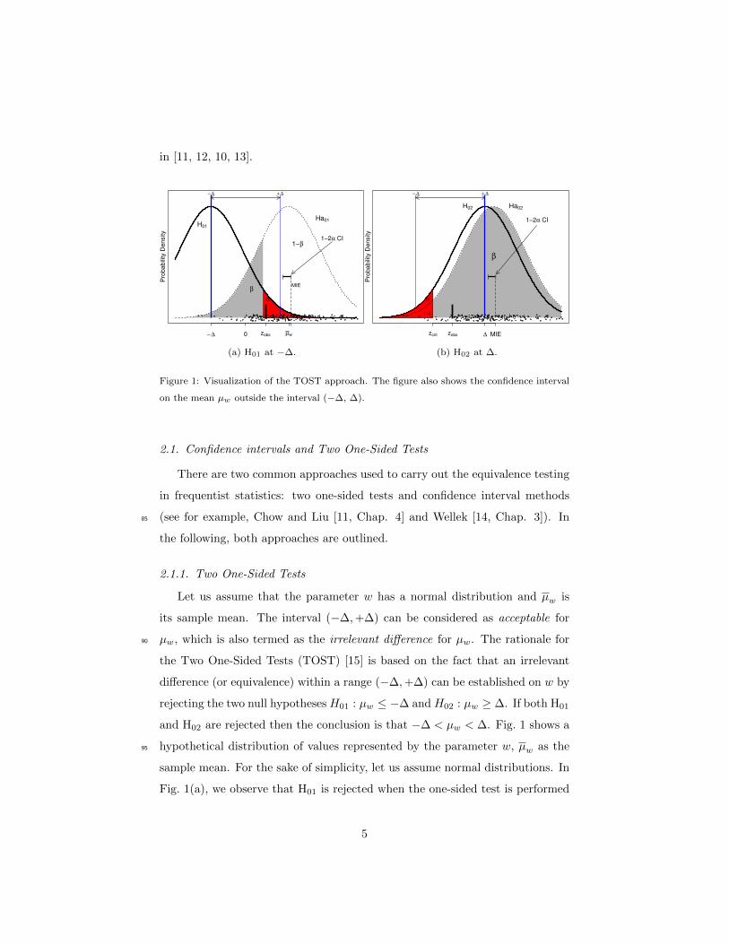
Figure 1: Visualization of the TOST approach. The figure also shows the confidence interval

on the mean µw outside the interval (−∆, ∆).

2.1. Confidence intervals and Two One-Sided Tests

There are two common approaches used to carry out the equivalence testing

in frequentist statistics: two one-sided tests and confidence interval methods

(see for example, Chow and Liu [11, Chap. 4] and Wellek [14, Chap. 3]). In85

the following, both approaches are outlined.

2.1.1. Two One-Sided Tests

Let us assume that the parameter w has a normal distribution and µw is

its sample mean. The interval (−∆,+∆) can be considered as acceptable for

µw, which is also termed as the irrelevant difference for µw. The rationale for90

the Two One-Sided Tests (TOST) [15] is based on the fact that an irrelevant

difference (or equivalence) within a range (−∆,+∆) can be established on w by

rejecting the two null hypotheses H01 : µw ≤ −∆ and H02 : µw ≥ ∆. If both H01

and H02 are rejected then the conclusion is that −∆ < µw < ∆. Fig. 1 shows a

hypothetical distribution of values represented by the parameter w, µw as the95

sample mean. For the sake of simplicity, let us assume normal distributions. In

Fig. 1(a), we observe that H01 is rejected when the one-sided test is performed

5

at −∆ (with the risk α, Type I Error, set at 0.05) because the observed value

from the data, zobs, is within the critical region. Therefore, it can be concluded

that the value represented by µw is of no practical importance. However, in100

Fig. 1 (b), when performing a t-test at +∆, it can be observed that H02 is not

rejected, therefore equivalence cannot be established. H02 is the null hypothesis

at ∆ and the observed value of the test, zobs, is outside the critical region, so

that the null hypothesis of inequivalence cannot be rejected.

2.1.2. Confidence Interval approach105

A procedure equivalent to the TOST method is the “confidence interval

approach” which basically checks whether the 1− 2α confidence interval of the

parameter under study lies within the range (−∆,+∆) [11, Chap. 4.2].

For illustration purposes, Fig. 1 shows the confidence interval on the mean for

the data of a parameter w. The parameter w has practical difference because the110

confidence interval is outside the interval (−∆,+∆). Had the confidence interval

lied within (−∆,+∆), the variable would have been considered to represent an

irrelevant difference.

Although the size 1 − 2α seems a logical consequence of the two one-side

tests, Berger and Hsu [16] reported different problems that could arise when115

generalizing the method to higher dimensions. The origin of the use of a con-

fidence interval for bioequivalence testing dates back to 1972 in an article by

Westlake [17]. However, the so-called “Westlake confidence intervals,” symmet-

ric around 0, are not in use nowadays due to their larger spans. There were

several discussions about the type of interval that should be computed for bioe-120

quivalence [18, 19, 15]. The conclusion is that the classical confidence interval

with length 1−2α for the mean difference should lie within the range (−∆,+∆)

in order to determine equivalence. The confidence interval approach is simple

to use and it avoids confusing the interpretation of the p-values of the statistical

tests, either under NHST or EHT.125

The principle of inclusion of the (1 − 2α) confidence interval within the

margins is one of the established criteria for showing equivalence and this is the

6

approach adopted in this work. In EHT, the margin limits constitute the range

that splits the regions of equivalence-inequivalence.

2.2. Bootstraping Confidence Intervals with the BCa130

An important element of our approach is to compute the confidence intervals

and to guarantee that they match the corresponding α-test. Since error distribu-

tions do not follow a normal distribution, bootstraping is applied, with the BCa

(bootstrap bias corrected and accelerated) being the recommended procedure.

The statistic bootstraped is the geometric mean, which is more appropriate to135

log-normal distributions than the standard mean.

The use of the bootstrap method for computing confidence intervals has

been applied by several authors in software engineering. A comparison of the

application and performance of the different types of confidence intervals in

software engineering is described by Lei and Smith [20]. These authors evaluated140

four bootstrap methods (Normal, Percentile, Student’s t and BCa) and observed

that the BCa behaved consistently across different software metrics, but the

procedure was not free of problems while computing some metrics.

Our present work does not intend to revise the application of bootstrapping

to the selected metric used (geometric mean of the absolute error), thus we145

apply to the standard BCa procedure. A brief description of the BCa method is

explained by Ugarte et al. [21, p. 473]. We report the BCa confidence interval

following their recommendations [21, Sec. 10.9]. A discussion about the different

approaches to the bootstrap of confidence intervals can be found in [22]. The

R [23] implementation of the bootstrap, boot.ci, guarantees an equi-tailed150

two-sided nonparametric confidence interval.

2.3. Using EHT for model comparison

Robinson et al. [24, 25] applied equivalence tests for validating prediction

models for forest growth measurements in the area of ecological modelling. The

authors’ starting position (null hypothesis) is that the model is unacceptable155

and it is the model that has to show some accuracy properties. Although they

7

reported a limited practical utility of their models, the authors showed a good

application of equivalence tests as a tool for model validation. As in the current

work, they also used bootstraped confidence intervals instead of model-based

ones since the assumption of normality could not be guaranteed.160

Among other works using EHT for validation purposes in other application

areas, Leites et al. [26] used equivalence tests for the assessment of different

forest growth models. Equivalence tests were used for validation of the bias,

which was defined as the mean of the error of measurements minus predictions.

The main benefit reported by these authors is that the “error of mistakenly165

validating the model is a Type I Error with a fixed probability.”

There are recent applications of EHT in the software engineering field. For

example, Borg and Pfahl [27] carried out an experiment with eight subjects to

compare two requirement traceability tools (Retro and ReqSmile) using EHT.

Dolado et al. [13] compared the results of several experimental crossover designs170

using EHT.

This work is restricted to study to the values of the absolute effort estimation

errors. To do so, confidence intervals for the geometric mean of those values are

calculated, because we are dealing with the absolute error between observations

yi and predictions yi, |yi−yi|. The objective is to find the method that minimizes175

the geometric mean of the absolute error (gMAR) without any specific interest

in any particular estimation in the dataset. We are only interested in setting

a limit for equivalence. The margin of equivalence is the smallest value that

would include the confidence interval. This value is the largest absolute value of

the extreme values of the confidence interval since establishing that value on the180

margins on −∆ and +∆ will make the confidence interval “equivalent” within

the limits. The principle of inclusion within a margin will be further described

in Section 3.1.

2.4. Other Types of Intervals

There are several works dealing with the evaluation of estimation models185

using other types of intervals, although those works are not in the line of EHT.

8

The use of the “Prediction Interval” for estimation purposes has been shown in

the works of [28, 29, 30], [31]. The purpose of a prediction interval is different

from that of a confidence interval. Heskes [32] shows the differences between

confidence intervals and prediction intervals. We refer the reader to [33, Chap-190

ter 3] for an explanation with examples about these differences. Mittas et al. [3]

have also constructed the tool StatREC that provides different types of graphical

intervals and statistical tests.

In Section 6, all data points generated by means of probability intervals are

evaluated, which are constructed from a Bayesian perspective.195

3. Measures of Accuracy

There are several ways to measure effect size and accuracy of an estimation

method. The most common measures used in the software estimation field are

the mean of the magnitude of the relative error (MMRE), the median mag-

nitude of the relative error (MdMRE) and the level of predicion at the 25%200

(LPred(0.25)). A list of the most used measures in other fields can be found in

[34, Section 2/5]. They include: root mean squared error (RMSE), mean abso-

lute percentage error (MAPE) and mean absolute scaled error (MASE). The list

of measures of accuracy can be extended further. For example, Cumming [35,

p. 39] describes a list of potential measures of effect size, such as difference205

of means, Cohen’s d, the correlation coefficient, etc., each one having specific

properties. The selection of one of these measures depends on several factors,

such as the field of application, measures previously used in the literature and

characteristics of the data.

The comparison of models using machine learning approaches has been a210

common topic of research since the early works comparing neural networks and

genetic programming [36, 37] to the recent systematic review [38]. All compar-

isons were performed primarily using the MMRE, Level of Prediction at 25%

and Median of the MRE. These measures have been used alone or in combina-

tion with different statistical tests. A list of problems related to the comparison215

9

of estimation methods can be found in [39]. Other issues related to effect size

and statistical power in estimation studies have also been reported by [40].

To overcome many of the problems of measuring forecasting accuracy in

times series data, Hyndman and Koehler [41] proposed to use the random esti-

mation as a reference point for computing the accuracy of an estimation. Their220

idea was to scale the error based on the mean absolute error with respect to the

naıve (random walk) point.

Shepperd and MacDonell clearly showed the inadequacy of the MMRE for

software estimates [7, Table 1]. Based on the idea of Hyndman and Koehler,

Shepperd and MacDonell defined a new measure in the field of software esti-225

mation called the Standardised Accuracy (SA), which is based on computing a

value using both the MAR and the random estimation, MARP0, as a reference

point:

SA = 1− MAR

MARP0

× 100. (1)

SA is defined between the values of 0 and 1 (or in percentage between 0%

and 100%). Using this measure, the authors concluded that the previous studies230

about the empirical evaluations of prediction systems are “unsafe.”

We review these concepts already established in software effort estimation

field to define a new measure that uses a specific point. That point is the upper

limit of a confidence interval of the gMAR. This has the advantage that the

evaluation is computed with a preset α level or Type I Error if H0 is true.235

3.1. Minimum Interval of Equivalence

In this Section, the ideas of the EHT for justifying the use of one of the

extreme points of a confidence interval as a reference point in a measure of

accuracy are described. The EHT procedure uses the margin limits ±∆ as

the reference points for checking whether or not the confidence interval of the240

mean lies in (−∆,+∆). When those margin limits are unavailable or have not

been defined, there is the possibility of computing those margins based on a

percentage over the mean or over another reference point. There are several

10

works that have used this approach as explained in Section 2.3. In any case, it

is possibe to use the equivalence confidence interval itself as a reference point245

for subsequent uses.

The concept of Minimum Interval of Equivalence (MIE) implies that if there

are no clear guidelines for setting the limits of the equivalence interval, one

may establish the smallest interval that includes the 1 − 2α confidence inter-

val. This is the minimum interval that rejects the null hypothesis of difference250

or inequivalence, and this is called the MIE. Reporting the MIE for validat-

ing a model provides the analyst with the idea of “how close the model was

to rejecting the null hypothesis of dissimilarity”. Robinson et al. [25, p.912]

concluded that the interval of equivalence can be used as a decision-making

tool. In this case, the burden of proof is put on the model since the starting255

assumption is “dissimilarity”. The authors suggested to use “the smallest in-

terval of equivalence that would still lead to rejection of the null hypothesis”.

As an example of application, Miranda et al. compared fire spread algorithms

using EHT [42] and reported the minimum interval of equivalence as “the small-

est interval that would lead to rejection of the null hypothesis of dissimilarity”260

(following [24, 25]). Units of MIE were proportions of the mean. Despite the

mixed results obtained, the authors found that the information provided by the

relative changes in average MIE [42, pp.595] was useful.

The concept of MIE was developed independently by Meyners [43, 10]. He

proposed to use “the Least Equivalent Allowable Difference (LEAD)” in equiv-265

alence testing for defining the smallest value for which equivalence could be

claimed. In this way, given a confidence interval with range (l, u), the largest

absolute value of l, u is the LEAD. The positive and negative LEAD values es-

tablish an interval in which the confidence interval is included. That interval is

the smallest region of equivalence that contains the confidence interval. Meyn-270

ers [10, Section 10] also found that “the LEAD is particularly useful in situations

in which the investigator was unable to choose an equivalence margin.”

In the current work, we follow these ideas about finding the confidence inter-

vals and the MIE (or LEAD) will be computed for each parameterised instance

11

of an estimation model. For a given method and dataset we consider as the275

best confidence interval the one that gives the best MIEu (the upper limit of

the interval). Afterwards we compute the corresponding MIEratio, which takes

into account the distance with respect to a random estimation. It means that

we do not compare the MIEu directly but we use the MIEratio, which is defined

in the next section. The use of the MIE concept is valuable since it allows us the280

comparison of limits irrespectively of any previous definition of the equivalence

margin. Also, it is important to remark that the MIEu value depends solely

on α, the Type I Error when the null hypothesis is true. Fig. 2 illustrates the

concept of the MIE. Given a distribution of residuals or errors – in this case the

absolute values are used– a confidence interval for the mean of those values is285

built. The largest value of the confidence interval sets the limit for equivalence;

hence, we can define the upper limit of the Minimum Interval of Equivalence.

It is interpreted in the sense of the following: if the limit +∆ had been set at

the MIEu we could have declared “equivalence.”

3.2. A New Measure of Accuracy: MIEratio290

In this section, a dimensionless measure based on the MIE is defined. The

main problem with the previous uses of the MIE is that it has been defined

with respect to the sample mean. Using the sample mean as a reference point

makes it difficult to compare different models on different datasets. This is

especially important in estimation models where the larger the error, the worse295

it is. Therefore, the concept of “random estimation” is used as part of the new

measure for effort estimation in a similar way to the Standardised Accuracy (SA)

proposed by Shepperd and MacDonell [7]. The random estimation value is used

as a reference point, as originally suggested by Hyndman [41] for measuring the

accuracy of time series. The reference point defined by Shepperd and MacDonell300

for software engineering data is denoted by MARP0.

The MARP0is defined as the “mean value of a large number runs of random

guessing”. It equates as predict a yi for the target case i by randomly sampling

over all the remaining n− 1 cases and take yi = yr, where r is drawn randomly

12

+ ∆

| |

0 ∆ MIE MARP0

1−2α CI

Minimum Equivalence Inequivalence

OMARP0

Figure 2: Plot of the 1 − 2α confidence interval of the Absolute Residuals (errors) and the

corresponding MIE. The MIEu is the value of the MIE that would lead to rejection of the null

hypothesis of dissimilarity.

from 1...n ∧ r 6= i (see [7, p. 222]). However, we use ”the exact MARP0“305

proposed by Langdon et al. [44] which consists in iterating over all n(n − 1)

different combinations of the n data elements and computing the mean of the

absolute error. In this way, we avoid ”randomness“.

Using both the MIEu and the reference point MARP0 , the MIEratio is

defined as:310

MIEratio =MIEu

(MARP0−MIEu)

(2)

which measures how far the method is from the random estimation, with respect

to the minimum range that sets the limit to equivalence. The lower the MIEratio

is, the better the estimation method is because it is closer to 0, i.e., further away

from MARP0. The MARP0

is constant for each dataset.

13

While in SA the range of values lies between 0 and 1, in the MIEratio the315

range of values goes from 0 to +∞. When the MIEratio is equal to 1 there is a

situation in which the estimations are equally distant from the perfect estimation

(value 0) and from the worst estimation (MARP0). Negative values of the

MIEratio are discarded. Values of the MIEratio approach the limit +∞ when

the value of the MIEu gets closer to MARP0, which represents bad estimations.320

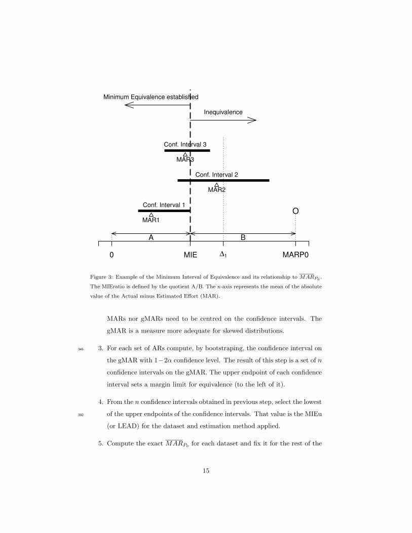
Fig. 3 shows a hypothetical situation in which we have obtained three con-

fidence intervals on the mean of the absolute value of the difference between

the actual and the estimated effort. In Fig. 3 it can be observed that the Con-

fidence Interval 1 (computed with a specific α) sets the limit for equivalence

and that the MIEratio is defined by the quotient A/B. From the EHT point of325

view, the A and B regions have an opposite interpretation, equivalence versus

inequivalence. The MIEratio is the variable reflecting that relationship.

Due to the fact that the MIEu splits the parameter space into two clear re-

gions with different interpretation (equivalence versus inequivalence, for a spe-

cific α), the MIEratio may be used as a measure for comparing estimation330

methods.

4. Experimental Work

The procedure that we will apply in the next sections is as follows:

1. Take a dataset that provides the Actual Effort of a project, split it in

three folds, and compute one or several n estimations (Estimation 1 to335

Estimation n for the dataset). The n different estimations are obtained

varying different parameters of the estimation method: adjusting con-

stants, adding factors or variables, etc.

2. Compute the Absolute Error, which we call it here Absolute Residual

(AR), for each estimation. This results in n sets of ARs. Each estimation340

will have a geometric Mean of the Absolute Residuals (gMAR). Fig. 3

shows the MAR for each confidence interval of the ARs. Note that neither

14

0 MIE ∆1 MARP0

OConf. Interval 1

MAR1

Conf. Interval 2

MAR2

Conf. Interval 3

MAR3

Inequivalence

Minimum Equivalence established

A B

Figure 3: Example of the Minimum Interval of Equivalence and its relationship to MARP0.

The MIEratio is defined by the quotient A/B. The x-axis represents the mean of the absolute

value of the Actual minus Estimated Effort (MAR).

MARs nor gMARs need to be centred on the confidence intervals. The

gMAR is a measure more adequate for skewed distributions.

3. For each set of ARs compute, by bootstraping, the confidence interval on345

the gMAR with 1−2α confidence level. The result of this step is a set of n

confidence intervals on the gMAR. The upper endpoint of each confidence

interval sets a margin limit for equivalence (to the left of it).

4. From the n confidence intervals obtained in previous step, select the lowest

of the upper endpoints of the confidence intervals. That value is the MIEu350

(or LEAD) for the dataset and estimation method applied.

5. Compute the exact MARP0for each dataset and fix it for the rest of the

15

computations.

6. Compute the MIEratio using both the MIEu value and the MARP0of the

previous steps.355

7. Repeat steps 1 to 6 for each dataset and for each fold.

8. Sort the results in ascending order of the MIEratio values. The closer the

result is to zero, the better the result is.

9. Group the MIEratio values by method, compute the probability intervals

and compare their distributions. The closer the result is to zero, the better360

the result is.

The previous procedure may be repeated for every dataset available and for

every estimation method that the analyst wishes to compare.

4.1. Machine Learning software effort estimation methods

The purpose of this work is to show how to compare software estimation365

methods using the MIEratio, therefore we have generated different software

effort estimates using different machine learning algorithms covering most rele-

vant types of techniques usually applied in the software estimation literature. As

there can be a high variability in the results depending on the parameters used

when applying machine learning methods, we have obtained multiple estimates370

varying the most important parameters of each technique.

Regression models Regression techniques are the most applied techniques to

estimate software effort and in this work we have applied the classical

Ordinary Least Squares (OLS) and Least Median Squared (LMS). These

techniques fit a multiple linear equation between a dependant variable375

(software estimation effort) with a set of or independent variables that

can be numeric or nominal such as the number of function points, team

size or the type of development platform.

16

The aim is to find, using matrix based operations, the slope coefficients of

a linear model y = β0 + β1x1 + β2x2 + ... + βkxk + e that minimises the380

square root error. In this work we have used Weka’s implementation [45].

Weka is a well-known machine learning software.

Instance based techniques In Instance Based techniques (IB-k), there is no

model as such to classify new samples, instead all training instances are

stored and the nearest instance(s) is/are retrieved to provide the class or385

calculate the estimate. In addition to different distance metrics used to

compare, other parameters that need to be considered include the number

of neighbours (k), use of weights with the attributes, normalisation of

the attributes, etc. This technique has been extensively applied by the

software engineering community as Case-based Reasoning (CBR) [46].390

Genetic Programming Genetic Programming (GP)[47, 48] is a type of evo-

lutionary computation technique in which free form equations evolve to

form a symbolic regression equation without assuming any distribution.

Several authors have reported on the suitability of using GP in software

effort estimation for over a decade [36]. In this work, we have used a395

canonical implementation based on Weka, which employs trees as a repre-

sentation and that it is capable of dealing with classification and regression

problems.

Neural Networks Neural networks (NN) are one of the classical machine

learning techniques applied to software effort estimation. NNs are com-400

posed of nodes and arcs organised in layers (usually an input layer, one

or two hidden layers and an output layer). Their arcs have weights to

control the propagation of the information that is propagated through

the network. There are multiple types of neural networks; the Multilayer

Perceptron (MLP) is one of the most popular type in which the informa-405

tion is propagated forward from the input layer composed of attributes

such as functional size to the output layer nodes (e.g., effort, time, etc.)

through one or more hidden layers. Weka’s MLP implementation is the

17

Multilayer Perceptron algorithm in which nodes are sigmoid except with

numeric classes in which case output nodes are unthresholded linear units.410

The loss function during training is the squared-error function.

Regression and model trees Classification and Regression Tress (CART) [49]

are binary trees which are induced minimising the subset variation at each

branch. In the case of numeric prediction, as it is our case, each leaf rep-

resents the average value of the training examples covered at that leaf.415

We have used Weka’s REPTree (Reduction-Error Pruning) [45] algorithm

for classification or regression. In the case of regression, variance is used

as a splitting criterion and the induced tree can be postpruned to both

simplify the tree and to avoid overfitting.

Model trees, originally proposed by Quilan as the M5 algorithm [50], are420

similar to regression trees but each leaf is composed of a regression equa-

tion instead of the average of the observations covered at each leaf, i.e.,

a linear regression model is induced with the observations of each leaf.

Weka’s M5P is a improvement of the original M5 algorithm.

In addition to the postpruning process there is also a smoothing process425

to avoid discontinuities between adjacent linear models. Model tree algo-

rithms should provide higher accuracy than regression trees but they are

also more complex.

4.2. Software Engineering Effort Datasets

We apply the methods described in the previous section on seven publicly430

available datasets. Two of them, China and ISBSG, have a relatively large

number of instances. A third one, the CSC dataset is more homogeneous as it

is composed of projects that belong to a single company. The Desharnais and

Maxwell datasets are well-known and can be found in the PROMISE repositories

1 and in [51], respectively. The two remaining datasets (Atkinson and Telecom1)435

1http://openscience.us/repo/effort/

18

are used to compare our results with the results available in the literature, in

particular with the results obtained by Shepperd and MacDonell [7].

CSC dataset The CSC data set [52], also known as Kitchenham’s data set, is

provided by a single company CSC and it is composed of 145 instances.

In our study we used the attributes duration, adjusted function points440

and first estimate as independent variables to estimate the Actual effort

(after running an attribute selection algorithm, these were found to be the

relevant attributes to deal with effort estimation). This was also the most

homogeneous dataset (all data belonged to a single company)

China dataset The China dataset is composed of 499 projects developed in445

China by various software organisation in multiple domains (cross-company

dataset). It has been used in several works, in particular by Menzies et

al. [53].

We found some issues with the original dataset and as a consequence we

carried out some preprocessing. The DevType attribute could not be used450

as the value of this attribute was zero for all instances. However, we could

differentiate between new developments and enhancements (or redevelop-

ments) if the number of function points of the Changed or Deleted field

was not zero. We did not use the productivity attributes as they were

directly derived from the class attribute (effort).455

The ISBSG dataset The International Software Benchmarking Standards Group

(ISBSG) [54] maintains a software project management repository from

multiple organisations.

In this work, we have used ISBSG v10 and it was also necessary to perform

some preprocessing in order to apply machine learning techniques, for se-460

lecting projects and attributes and for cleaning the data (the preprocessing

carried out in this dataset is explained in detail in [55]).

Atkinson and Telecom1 datasets Although the Atkinson and Telecom1 datasets

are very small datasets (at least for data mining purposes), these have

19

been extensively used in the past for assessing the estimation-by-analogy465

method, regression-to-the-mean and other methods.

The Atkinson dataset contains 16 data points relating real-time function

points to effort. The Telecom1 dataset contains 18 points relating effort

to changes in the configuration management and number of files changed

during the development of a software system [46, 56].470

The Atkinson dataset is reproduced in full in Appendix B of [56]. The

authors report that some cases were removed from the analysis based on

the homogeneity of the projects. The 16 points of this dataset have been

used for computing the SA (see Table 2 of [7]). The Telecom1 dataset

is available in Appendix A of [56] and in Appendix A [46]. It contains475

18 data points. This dataset was used for comparing EBA to step-wise

regression, among other methods. In these two datasets, we only use

the Actual Effort and Estimated Effort variables for computing the MIE,

gMAR, etc.

Maxwell dataset The Maxwell dataset [51] is composed of 63 projects and the480

following attributes: application size (in Function Points), effort in hours,

duration in months. It also provides 21 discrete attributes (applicaytion

type, hardware platform, DBMS architecture, user interface, language(s)

used, and other 15 attributes using the Likert scale about the development

environment characteristics. Although this dataset suffers from the curse485

of dimensionality as there is a large number of attributes compared with

the number of instances, we used all attributes with the exception of the

project starting date.

4.3. Data Analysis

All previously described machine learning algorithms are implemented in490

Weka [45] and they were used to obtain sets of effort estimates per technique

(with the exception of the Atkinson and Telecom1 datasets as explained previ-

ously). In order to ensure that the same instances were used for training and

20

testing in each technique, we partitioned each dataset into three folds using

stratified sampling before applying the machine learning algorithms. Stratified495

sampling ensures a random sampling following the distribution of the class (ef-

fort attribute). We used 2 folds for training (2/3 of the instances) and and 1

fold for testing (1/3 of the instances) and repeat the procecedure three time so

that all data points were used for training and testing and to have more points

for further analysis. This is in line with the work by Mittas and Angelis [57].500

Each machine learning technique was run varying combinations of different

parameters to induce a set of different estimates per method (except for the

Atkinson and Telecom1 datasets in which the results are those provided in their

respective publications). Table 1 shows the parameters modified per method and

their respective range. In the case of regression with Ordinary Least Squares505

(OLS), it is possible to vary the ridge parameter (this variation only minimally

affects the output) and whether Feature Selection (FS) is used to generate the

model. The FS method can be based on the M5 model tree (M5P) which removes

attributes until there is no improvement. With Least Median Squared (LMS),

it is possible to induce multiple models varying the size of the sample (S) used510

to generate the regressions. For the GP, we obtained different estimates varying

the size of the population (pop) and number of generations that we allowed the

algorithm to run (com). We only allowed arithmetic operators, exponential and

logarithms excluding logical (if, and, or) and functions (min, max). In all cases

the fitness function selected was the Root Mean Square Error (RMSE).515

In the case of IBk, there is also a large number of possible parameters but we

varied the number of neighbours (k) and the function distance used (Euclidean

or Manhattan). For regression and model trees, with the REPTree algorithm

(regression tree), the parameters were minimum proportion of the variance on

all the data that needs to be present at a node for splitting (V ), the number520

of folds (N) which determines the amount of data used for pruning (one fold

is used for pruning, the rest for growing the rules) and minimum total weight

of the instances in a leaf (M). In the case of M5P (model tree), the parameter

modified was the minimum number of instances allowed at a leaf node (M). For

21

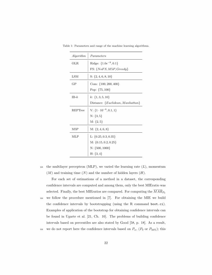
Table 1: Parameters and range of the machine learning algorithms.

Algorithm Parameters

OLR Ridge: {1.0e−8, 0.1}

FS: {NoFS,M5P,Greedy}

LSM S: {2, 4, 6, 8, 10}

GP Com: {100, 200, 400}

Pop: {75, 100}

IB-k k: {1, 3, 5, 10}

Distance: {Euclidean,Manhattan}

REPTree V: {1 · 10−8, 0.1, 1}

N: {3, 5}

M: {2, 5}

M5P M: {2, 4, 6, 8}

MLP L: {0.25, 0.3, 0.35}

M: {0.15, 0.2, 0.25}

N: {500, 1000}

H: {3, 4}

the multilayer perceptron (MLP), we varied the learning rate (L), momentum525

(M) and training time (N) and the number of hidden layers (H).

For each set of estimations of a method in a dataset, the corresponding

confidence intervals are computed and among them, only the best MIEratio was

selected. Finally, the best MIEratios are compared. For computing the MARP0

we follow the procedure mentioned in [7]. For obtaining the MIE we build530

the confidence intervals by bootstrapping (using the R command boot.ci).

Examples of application of the bootstrap for obtaining confidence intervals can

be found in Ugarte et al. [21, Ch. 10]. The problems of building confidence

intervals based on percentiles are also stated by Good [58, p. 18]. As a result,

we do not report here the confidence intervals based on Pα, (P0 or P50%); this535

22

option could be justified in the work by Shepperd and MacDonell [7] since their

histograms showed symmetry.

Absolute Residuals (Errors)

Fre

qu

en

cy

0 2000 4000 6000 8000

05

01

00

15

0

(a) China dataset using the M5P method.

Absolute Residuals (Errors)

Fre

qu

en

cy

0 10000 20000 30000 40000 50000

05

01

00

15

02

00

(b) ISBSG dataset using the IBK method.

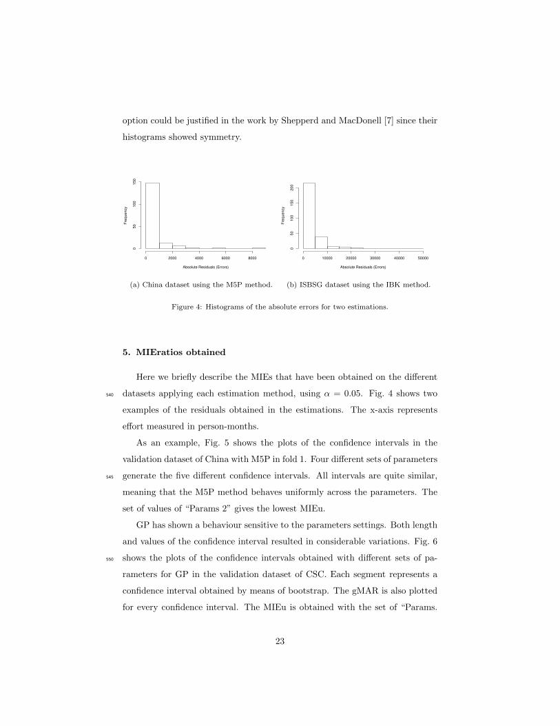
Figure 4: Histograms of the absolute errors for two estimations.

5. MIEratios obtained

Here we briefly describe the MIEs that have been obtained on the different

datasets applying each estimation method, using α = 0.05. Fig. 4 shows two540

examples of the residuals obtained in the estimations. The x-axis represents

effort measured in person-months.

As an example, Fig. 5 shows the plots of the confidence intervals in the

validation dataset of China with M5P in fold 1. Four different sets of parameters

generate the five different confidence intervals. All intervals are quite similar,545

meaning that the M5P method behaves uniformly across the parameters. The

set of values of “Params 2” gives the lowest MIEu.

GP has shown a behaviour sensitive to the parameters settings. Both length

and values of the confidence interval resulted in considerable variations. Fig. 6

shows the plots of the confidence intervals obtained with different sets of pa-550

rameters for GP in the validation dataset of CSC. Each segment represents a

confidence interval obtained by means of bootstrap. The gMAR is also plotted

for every confidence interval. The MIEu is obtained with the set of “Params.

23

0 1061.01 3929

MIE MARP0

753.08 1063.01

Params. 1

gMAR

752.81 1061.01

Params. 2

gMAR

753.44 1073.94

Params. 3

gMAR

752 1068.11

Params. 4

gMAR

OMARP0

Figure 5: Confidence intervals and the Minimum Intervals of Equivalence for the M5P method

applied to the China dataset in fold 1.

5” and it is shown with the vertical dotted line: there is no other smaller value

that contains a confidence interval.555

The application of neural networks has shown a large variation in the size

and location of the confidence intervals depending on the parameters used for

adjusting the NNs.

The lowest MIEu values for every dataset and method applied were selected.

Visual inspection of the MIEu values does not help to determine which of the560

methods has performed the best since theMARP0s are different for each dataset.

Therefore, the dimensionless MIEratio will help us to establish which of the

confidence intervals performs best with respect to the random estimation.

Table 2 shows a subset of the values obtained, using α = 0.05, sorted in

ascending order by the MIEratio, from the lowest value (best method) up to the565

highest (worst) value. Each row of the table contains the computed values for

a specific estimation method and a dataset.

The list of methods shown in the first column are: genetic programming

(GP), IB-k for case-based reasoning, Ordinary Least Squares (LR) and Least

Median Square (LMS) for linear regressions, Multilayer Perceptron (MLP) for570

24

0 280.09 2292

MIE MARP0

372.1 608.5

Params. 1

gMAR

381.97 544.34

Params. 2

gMAR

376.81 543.8

Params. 3

gMAR

137 301.32

Params. 4

gMAR

136.75 280.09

Params. 5

gMAR

218.54 358.69

Params. 6

gMAR

OMARP0

Figure 6: Confidence intervals and the Minimum Intervals of Equivalence for GP and CSC in

fold 2.

neural networks, model trees (M5P) and RTree for regression trees. The next

columns show the MMRE, MdMRE, Level of prediction and the MIE. The

column SA is the “standardised accuracy” of Shepperd and MacDonell. The

MIEratio is the criterion used for sorting the table. Therefore, this table com-

pares the most usual measures of accuracy using the MIEratio as the reference.575

It can be observed that the order obtained in the last column is not main-

tained in the rest of the columns. In this situation the main advantage of the

MIEratio is that it is computed with a fixed known α, which is essential when

comparing estimates obtained from different datasets. The ordering of values

that are not matched between the SA and the MIEratio are shown in italics in580

the column SA.

When establishing an ordering among the estimation methods based on the

MIEratio as an accuracy metric, it is observed that the datasets themselves were

25

the main grouping variable in the ordering. This result is in line with some

conclusions reported by other authors [57, 59], with respect to the importance585

of the data itself.

6. Evaluation of the Methods with Probability Intervals

The final question “Which is the best estimation method?” can stated as

“which method provides a probability of the MIEratio closer to 0?.” A good

method should have generated a set of values as close to 0 as possible with590

respect to the random estimation. The data grouped by method provide a

source for making these inferences.

In order to compare the methods, the data of the MIEratios is grouped by

method and different probability intervals are constructed for each method. The

data that we can use to select an estimation method as the best candidate are595

the values of the MIEratio obtained in the previous sections. In our case there

are 5 datasets (not including the Atkinson and Telecom datasets) multiplied by

number of folds (3), that is, a total of 15 data points per method. Had we not

splitted the datasets into 3-folds, the number of data points that corresponds

to the number of datasets would be very low (5) for the analysis. We consider600

the data of the MIEratios “observational”, hence it is reasonable to generate a

probability interval that describes the data distribution.

Probabily intervals are different from confidence intervals. Confidence inter-

vals are constructed from a frequentist point of view. The concept of “probabil-

ity interval” comes from the area of Bayesian inference. A probability interval,605

usually called “credible interval”, is a range of values in which we can be certain

that the parameter falls with a given probability. A 95% credible interval is the

range of values in which we are 95% certain that the parameter θ of interest

falls (e.g. the MIEratio, a mean or other). On the other hand, a frequentist

confidence interval does not convey a probability distribution. A frequentist610

confidence interval is based on the long-run frequency of the events. Frequentist

confidence intervals are computed with the sample data; the procedure guaran-

26

tees that in the long run a specific percentage of them (e.g. 95%) will contain

the true value of the parameter.

Frequentist and Bayesian methods approach the construction of intervals in615

different ways, because their purpose and aim are different. A Bayesian credible

interval is a posterior probability that the parameter lies within the interval

constructed. The reader may refer to [60, 61] for a detailed explanation of the

differences betweem frequentism and bayesianism.

For our purposes, it suffices to say that a 95% confidence interval is a set of620

values constructed in such a way that 95% of such intervals will contain the true

value of the population and a credible interval is a set of values that represent

the probability that the parameter under study will lie within the interval. This

probability is computed after the data is observed.

A detailed comparison of the construction between these two types of inter-625

vals is described by Cowles [62, Chapter 4] and a description of the construction

of probability intervals can be found in Neapolitan’s book [63, Section 6.3]. The

Bayesian technique is most adequate to make inferences with few data points.

It is the interpretation that we are interested in because it is the probability

that the true value of the parameter (θ) is in the interval. In some situations630

both types of intervals (confidence and credible) may provide similar or equal

values, but their interpretation is different.

Given the data provided by the MIEratios and grouped by method, we com-

pute three types of Bayesian intervals with the LaplacesDemon package for

R [64] and other R code.635

� A quantile-based interval that computes a 95% probability interval, given

the marginal posterior samples of θ. It is simply the 2.5% and 97.5%

quantiles of the samples for the distribution. It doesn’t take the prior

distribution into account.

� The Highest Posterior Density intervals (HPD), recommended for asym-640

metric distributions. It is the shortest possible interval enclosing (1−α)%

of the distribution. This interval doesn’t take the prior distribution into

27

account.

� Credible interval based on Metropolis-Hastings sampling with the use of

the non-informative Jeffreys prior for a lognormal model, using the R code645

of 2

Table 3 shows the intervals computed, using α = 0.05. It can be observed

that the best HPD intervals are those of GP. LMS provides good results too.

By comparing the values of the intervals in Tables 3 and 5 we see more discrim-

inative power in table 3 due to the scale. Hence, this being the benefit of the650

current approach.

Table 4 shows the credible intervals for the means of 10 runs, in order to

have a perception of how the methods work under different splits of the data.

Each run involves variation of all parameters and a different seed for dividing

the datasets.655

Fig. 7 shows the HPDs for each method. The black areas in the figures

represent the 95% probability that the true value of the MIEratio will fall within

the interval. The values of the HPDs are those of the second column in Table 3.

7. Threats to Validity

There are some threats to validity that need to be considered in this study.660

Construct validity is the degree to which the variables used in the study ac-

curately measure the concepts they are supposed to measure. The datasets

analyzed here have been extensively used to study effort estimation and other

software engineering issues. However, the data is provided “as it is.” There is

also a risk in the way that the preprocessing of the datasets was performed but665

it is common to find such approaches in the literature. Furthermore, the aim

of this paper is to show how the EHT approach makes it possible to define the

MIEratio and to examine what their probability distributions are. Organisa-

tions should select and perform the studies and estimations with subsets of the

2http://stats.stackexchange.com/a/33395

28

data close to their domain and organisation since there is no clear agreement if670

cross organisations data can ensure acceptable estimates.

Internal validity is the degree to which conclusions can be drawn. The hold-

out approach used could be improved with more complex approaches such as

cross validation or “leave one out” validation. A much further range of parame-

ters could have been used to obtain the estimates. However, the computational675

time makes this difficult in practice. We selected the most important param-

eters of the algorithms and we used ranges to ensure enough variability of the

estimates.

8. Conclusions

This work has shown an analysis of the predictive capabilities of different680

estimation algorithms from the perspective of Equivalence Hypothesis Testing in

the context of software effort estimation. The dimensionless measure MIEratio,

which is independent of the units of measurements, was defined as a criterion

for the assessment of evaluation models.

A probability distribution for each method was generated by grouping all685

MIEratios by method. These distributions answer the question: How close is

the method to the best estimation? The final goal in the estimation task would

be to have a perfect estimation, i.e., the absolute residual is 0. Therefore, the

lower the MIEratio is the closer we are to 0. The limit for improvement lies

at 0, which is the point where the estimations match the actual values and690

where there is no room for further improvement. The scale (0−∞) used in the

MIEratios allows a more clear identification of the differences.

According to the experimental simulations, the best intervals among all

techniques, obtained by comparing the High Posterior Density intervals in the

datasets used, are those of the genetic programming technique and of the linear695

regression with least mean squares.

29

Acknowledgements

Partial support has been received by Project Iceberg FP7-People-2012-IAPP-

324356 (D. Rodriguez) and Project TIN2013-46928-C3 (D. Rodriguez and J.J.

Dolado) and EPSRC. The authors are thankful to Mannu Satpathy for his valu-700

able comments.

References

[1] A. Arcuri, L. Briand, A practical guide for using statistical tests to assess

randomized algorithms in software engineering, in: 33rd International Con-

ference on Software Engineering (ICSE’11), ACM, New York, NY, USA,705

2011, pp. 1–10.

[2] J. Derrac, S. Garcıa, D. Molina, F. Herrera, A practical tutorial on the use

of nonparametric statistical tests as a methodology for comparing evolu-

tionary and swarm intelligence algorithms, Swarm and Evolutionary Com-

putation 1 (2011) 3–18.710

[3] N. Mittas, I. Mamalikidis, L. Angelis, A framework for comparing multiple

cost estimation methods using an automated visualization toolkit, Infor-

mation and Software Technology 57 (2015) 310–328.

[4] C. Catal, Performance evaluation metrics for software fault prediction stud-

ies, Acta Polytechnica Hungarica 9 (4) (2012) 193–206.715

[5] R. Nuzzo, Statistical errors, Nature 506 (7487) (2014) 150–152.

[6] C. Woolston, Psychology journal bans p values, Nature 519 (2015) 9.

[7] M. Shepperd, S. MacDonell, Evaluating prediction systems in software

project estimation, Information and Software Technology 54 (8) (2012)

820–827.720

[8] E. Stensrud, T. Foss, B. Kitchenham, I. Myrtveit, An empirical validation

of the relationship between the magnitude of relative error and project size,

30

in: Eighth IEEE Symposium on Software Metrics (Metrics’02), 2002, pp.

3–12.

[9] T. Foss, E. Stensrud, B. Kitchenham, I. Myrtveit, A simulation study of725

the model evaluation criterion mmre, IEEE Transactions on Software En-

gineering 29 (11) (2003) 985–995.

[10] M. Meyners, Equivalence tests – a review, Food Quality and Preference

26 (2) (2012) 231–245.

[11] S.-C. Chow, J.-P. Liu, Design and Analysis of Bioavailability and Bioequiv-730

alence Studies, Chapman&Hall, 2009.

[12] D. Hauschke, V. Steinijans, I. Pigeot, Bioequivalence Studies in Drug De-

velopment. Methods and Applications, John Wiley & Sons, 2007.

[13] J. J. Dolado, M. C. Otero, M. Harman, Equivalence hypothesis testing in

experimental software engineering, Software Quality Journal 22 (2) (2014)735

215–238.

[14] S. Wellek, Testing statistical hypotheses of equivalence and noninferiority,

2nd Edition, Chapman & Hall, Boca Raton, Florida, USA, 2010.

[15] D. J. Schuirmann, A comparison of the two one-sided tests procedure and

the power approach for assessing the equivalence of average bioavailability,740

Journal of Pharmacokinetics and Biopharmaceutics 15 (6) (1987) 657–680.

[16] R. L. Berger, J. C. Hsu, Bioequivalence trials, intersection-union tests and

equivalence confidence sets, Statistical Science 11 (4) (1996) 283–302.

[17] W. J. Westlake, Use of confidence intervals in analysis of comparative

bioavailability trials, Journal of Pharmaceutical Sciences 61 (8) (1972)745

1340–1341.

[18] W. J. Westlake, Symmetrical confidence intervals for bioequivalence trials,

Biometrics 32 (4) (1976) 741–744.

31

[19] T. B. Kirkwood, W. Westlake, Bioequivalence testing–a need to rethink,

Biometrics 37 (3) (1981) 589–594.750

[20] S. Lei, M. R. Smith, Evaluation of several nonparametric bootstrap meth-

ods to estimate confidence intervals for software metrics, IEEE Transactions

on Software Engineering 29 (11) (2003) 996–1004.

[21] M. D. Ugarte, A. F. Militino, A. T. Arnholt, Probability and Statistics

with R, CRC Press, 2008.755

[22] B. Efron, Better bootstrap confidence intervals, Journal of the American

Statistical Association 82 (397) (1987) 171–185.

[23] R Core Team, R: A Language and Environment for Statistical Computing,

R Foundation for Statistical Computing, Vienna, Austria (2015).

URL http://www.R-project.org/760

[24] A. P. Robinson, R. E. Froese, Model validation using equivalence tests,

Ecological Modelling 176 (3-4) (2004) 349–358.

[25] A. P. Robinson, R. A. Duursma, J. D. Marshall, A regression-based equiv-

alence test for model validation: shifting the burden of proof, Tree Physi-

ology 25 (2005) 903–913.765

[26] L. P. Leites, A. P. Robinson, N. L. Crookston, Accuracy and equivalence

testing of crown ratio models and assessment of their impact on diameter

growth and basal area increment predictions of two variants of the forest

vegetation simulator, Canadian Journal of Forest Research 39 (2009) 655–

665.770

[27] M. Borg, D. Pfahl, Do better ir tools improve the accuracy of engineers

traceability recovery?, in: Proceedings of the International Workshop on

Machine Learning Technologies in Software Engineering (MALETS ’11),

2011, pp. 27–34.

32

[28] M. Jørgensen, K. H. Teigen, K. Moløkken, Better sure than safe? over-775

confidence in judgement based software development effort prediction in-

tervals, Journal of Systems and Software 70 (1) (2004) 79–93.

[29] N. Mittas, L. Angelis, Bootstrap prediction intervals for a semi-parametric

software cost estimation model, in: Software Engineering and Advanced

Applications, 2009. SEAA’09. 35th Euromicro Conference on, IEEE, 2009,780

pp. 293–299.

[30] N. Mittas, Evaluating the performances of software cost estimation models

through prediction intervals, Journal of Engineering Science and Technol-

ogy Review 4 (3) (2011) 266–270.

[31] M. Klas, A. Trendowicz, Y. Ishigai, H. Nakao, Handling estimation uncer-785

tainty with bootstrapping: Empirical evaluation in the context of hybrid

prediction methods, in: International Symposium on Empirical Software

Engineering and Measurement (ESEM 2011), IEEE, 2011, pp. 245–254.

[32] T. Heskes, Practical confidence and prediction intervals, Advances in neural

information processing systems (1997) 176–182.790

[33] D. R. Helsel, R. M. Hirsch, Statistical methods in water resources, Vol.

323, US Geological survey Reston, Va., 2002.

[34] R. Hyndman, G. Athanasopoulos, Forecasting: principles and practice,

2013, accessed on April, 2013.

URL http://otexts.com/fpp/795

[35] G. Cumming, Understanding the New Statistics: Effect Sizes, Confidence

Intervals, and Meta-Analysis, Routled, 2011.

[36] J. J. Dolado, L. Fernandez, Genetic programming, neural networks and

linear regression in software project estimation, in: C. Hawkins, M. Ross,

G. Staples, J. B. Thompson (Eds.), International Conference on Software800

Process Improvement, Research, Education and Training, British Com-

puter Society, London, 1998, pp. 157–171.

33

[37] J. J. Dolado, On the problem of the software cost function, Information

and Software Technology 43 (1) (2001) 61–72.

[38] J. Wen, S. Li, Z. Lin, Y. Hu, C. Huang, Systematic literature review of805

machine learning based software development effort estimation models, In-

formation and Software Technology 54 (1) (2012) 41–59.

[39] T. Menzies, M. Shepperd, Special issue on repeatable results in software

engineering prediction, Empirical Software Engineering 17 (1) (2012) 1–17.

[40] V. Kampenes, T. Dyba, J. Hannay, D. Sjøberg, A systematic review of810

effect size in software engineering experiments, Information and Software

Technology 49 (11) (2007) 1073–1086.

[41] R. J. Hyndman, A. B. Koehler, Another look at measures of forecast accu-

racy, International Journal of Forecasting 22 (4) (2006) 679–688.

[42] B. Miranda, B. Sturtevant, J. Yang, E. Gustafson, Comparing fire spread815

algorithms using equivalence testing and neutral landscape models, Land-

scape Ecology 24 (2009) 587–598.

[43] M. Meyners, Least equivalent allowable differences in equivalence testing,

Food Quality and Preference 18 (2007) 541–547.

[44] W. Langdon, J. Dolado, F. Sarro, M. Harman, Exact mean absolute error of820

baseline predictor marp0, Information and Software Technology, accepted

for publication.

[45] I. Witten, E. Frank, M. Hall, Data Mining: Practical machine learning tools

and techniques, 3rd Edition, Morgan Kaufmann, San Francisco, 2011.

[46] M. Shepperd, C. Schofield, Estimating software project effort using analo-825

gies, IEEE Transactions on Software Engineering 23 (11) (1997) 736–743.

[47] W. B. Langdon, R. Poli, Foundations of Genetic Programming, Springer,

2001.

34

[48] R. Poli, W. B. Langdon, N. F. Mcphee, A Field Guide to Genetic Program-

ming, no. March, Lulu, 2008.830

URL http://www.gp-field-guide.org.uk/

[49] L. Breiman, J. Friedman, R. Olshen, C. Stone, Classification and Regres-

sion Trees, Chapman and Hall (Wadsworth and Inc.), 1984.

[50] J. Quinlan, Learning with continuous classes, in: Proceedings of the 5th

Australian Joint Conference on Artificial Intelligence, 1992, pp. 343–348.835

[51] K. Maxwell, Applied Statistics for Software Managers, Software Quality

Institute Series, Prentice Hall PTR, 2002.

[52] B. Kitchenham, S. L. Pfleeger, B. McColl, S. Eagan, An empirical study

of maintenance and development estimation accuracy, Journal of Systems

and Software 64 (1) (2002) 57–77.840

[53] T. Menzies, A. Butcher, A. Marcus, T. Zimmermann, D. Cok, Local vs.

global models for effort estimation and defect prediction, in: Proceed-

ings of the 2011 26th IEEE/ACM International Conference on Automated

Software Engineering, ASE’11, IEEE Computer Society, Washington, DC,

USA, 2011, pp. 343–351.845

[54] C. Lokan, T. Wright, P. Hill, M. Stringer, Organizational benchmarking

using the isbsg data repository, IEEE Software 18 (5) (2001) 26 –32.

[55] D. Rodriguez, M. Sicilia, E. Garcia, R. Harrison, Empirical findings on

team size and productivity in software development, Journal of Systems

and Software 85 (3) (2012) 562–570.850

[56] S. Barker, M. Shepperd, M. Aylett, The analytic hierarchy process and

data-less prediction, Empirical Software Engineering Research Group ES-

ERG: TR98-04.

[57] N. Mittas, L. Angelis, Ranking and clustering software cost estimation

models through a multiple comparisons algorithm, IEEE Transactions on855

Software Engineering 39 (4) (2013) 537–551.

35

[58] P. I. Good, Resampling methods: a practical guide to data analysis, 3rd

Edition, Birkhauser, 2006.

[59] M. Shepperd, G. Kadoda, Comparing software prediction techniques us-

ing simulation, IEEE Transactions on Software Engineering 27 (11) (2001)860

1014–1022.

[60] J. VanderPlas, Frequentism and bayesianism: A python-driven primer,

arXiv preprint arXiv:1411.5018.

[61] E. Jaynes, O. Kempthorne, Confidence intervals vs bayesian intervals, in:

W. Harper, C. Hooker (Eds.), Foundations of Probability Theory, Statisti-865

cal Inference, and Statistical Theories of Science, Vol. 6b of The University

of Western Ontario Series in Philosophy of Science, Springer Netherlands,

1976, pp. 175–257.

[62] M. K. Cowles, Applied Bayesian statistics: with R and OpenBUGS exam-

ples, Vol. 98, Springer Science & Business Media, 2013.870

[63] R. E. Neapolitan, Learning bayesian networks, Vol. 38, Prentice Hall Upper

Saddle River, 2004.

[64] S. LLC, LaplacesDemon: Complete Environment for Bayesian Inference, r

package version 15.03.19 (2015).

URL http://www.bayesian-inference.com/software875

36

Method Dataset MARP0 MAR gMAR MMRE MdMRE Prd(0.25) MIE SA MIEratio

GP CSC(fld3) 7519.422 1272.354 59.737 0.222 0.136 0.646 209.463 0.831 0.029

LMS CSC(fld3) 7519.422 1336.410 275.156 0.220 0.153 0.625 407.243 0.822 0.057

M5P CSC(fld3) 7519.422 1545.455 305.637 0.260 0.202 0.604 463.690 0.794 0.066

LR CSC(fld3) 7519.422 1288.356 380.422 0.240 0.215 0.583 524.176 0.829 0.075

IBk CSC(fld3) 7519.422 3102.979 380.758 0.254 0.212 0.625 583.324 0.587 0.084

MLP CSC(fld3) 7519.422 2675.423 445.082 0.354 0.225 0.583 623.923 0.644 0.090

RTree CSC(fld3) 7519.422 3394.569 437.664 0.306 0.219 0.562 676.952 0.549 0.099

IBk CSC(fld2) 1315.700 274.729 141.111 0.219 0.165 0.646 189.628 0.791 0.168

LMS CSC(fld2) 1315.700 301.627 141.407 0.236 0.155 0.646 197.306 0.771 0.176

GP CSC(fld1) 2017.656 542.959 134.381 0.314 0.140 0.653 308.481 0.731 0.180

MLP CSC(fld1) 2017.656 571.323 219.519 0.465 0.165 0.694 319.590 0.717 0.188

LMS CSC(fld1) 2017.656 546.280 230.030 0.320 0.173 0.673 323.538 0.729 0.191

IBk CSC(fld1) 2017.656 563.694 241.057 0.324 0.187 0.694 333.918 0.721 0.198

M5P CSC(fld2) 1315.700 334.908 161.968 0.250 0.183 0.667 218.669 0.745 0.199

GP CSC(fld2) 1315.700 322.417 126.383 0.254 0.212 0.562 221.680 0.755 0.203

M5P CSC(fld1) 2017.656 668.263 247.102 0.320 0.159 0.694 352.094 0.669 0.211

MLP CSC(fld2) 1315.700 326.409 175.741 0.273 0.211 0.625 231.912 0.752 0.214

LMS ISBSG(fld3) 4721.474 2335.299 733.073 1.530 0.522 0.211 841.655 0.505 0.217

M5P ISBSG(fld1) 4479.924 1751.388 703.342 1.600 0.488 0.277 801.238 0.609 0.218

GP ISBSG(fld3) 4721.474 2385.943 719.476 0.970 0.607 0.192 846.011 0.495 0.218

M5P ISBSG(fld3) 4721.474 1987.367 749.641 1.688 0.546 0.265 857.184 0.579 0.222

M5P Maxwell(fld2) 12164.000 4134.663 1275.744 0.426 0.289 0.381 2298.224 0.660 0.233

LMS China(fld3) 5819.186 2588.090 930.265 1.006 0.572 0.229 1132.295 0.555 0.242

LMS ISBSG(fld1) 4479.924 2306.632 760.563 2.153 0.586 0.226 878.556 0.485 0.244

GP ISBSG(fld1) 4479.924 2322.634 745.572 0.938 0.586 0.192 883.946 0.482 0.246

LMS ISBSG(fld2) 3496.595 1782.202 625.202 1.280 0.478 0.240 721.919 0.490 0.260

GP China(fld2) 4446.223 2274.440 771.991 0.743 0.609 0.223 939.076 0.488 0.268

M5P China(fld3) 5819.186 2756.619 1056.587 1.352 0.591 0.193 1287.121 0.526 0.284

RTree ISBSG(fld3) 4721.474 2258.100 923.286 1.927 0.581 0.208 1048.239 0.522 0.285

LMS China(fld1) 4441.700 2267.206 836.736 1.029 0.512 0.228 1005.057 0.490 0.292

Table 2: This table shows the summary results for the best 30 values in ascending order of

MIEratio (α = 0.05).

37

Qtle. 2.5%-97.5% HPD low-upper M-Hast. 2.5%-97.5%

GP 0.082-1.057 0.029-1.304 0.279-0.787

IBk 0.114-1.658 0.084-2.06 0.354-0.891

LMS 0.099-1.261 0.057-1.673 0.267-0.645

LR 0.147-1.409 0.075-1.577 0.409-1.005

M5P 0.112-0.806 0.066-0.908 0.275-0.585

MLP 0.12-1.207 0.09-1.356 0.367-0.971

RTree 0.16-15.242 0.099-21.263 0.895-7.867

Table 3: This table shows different probabilistic intervals for each one of the 7 methods

(α = 0.05) for the data of the MIEratios. Scale is 0-∞. Lower values are better.

Qtle. 2.5%-97.5% HPD low-upper M-Hast. 2.5%-97.5%

GP 0.108-0.749 0.1-0.764 0.316-0.691

IBk 0.118-0.81 0.114-0.85 0.362-0.781

LMS 0.113-0.691 0.106-0.724 0.27-0.559

LR 0.23-3.123 0.204-3.808 0.582-1.586

M5P 0.128-0.778 0.125-0.82 0.3-0.595

MLP 0.182-1.647 0.145-1.99 0.461-0.978

RTree 0.334-1.962 0.329-2.022 0.775-1.837

Table 4: This table shows different probabilistic intervals for each one of the 7 methods

(α = 0.05) for the means of the MIEratios in 10 runs. Scale is 0-∞. Lower values are better.

38

Qtle. 2.5%-97.5% HPD low-upper M-Hast. 2.5%-97.5%

GP 0.289-0.804 0.217-0.831 0.47-0.672

IBk 0.307-0.766 0.297-0.791 0.449-0.597

LMS 0.417-0.804 0.38-0.822 0.519-0.643

LR 0.29-0.763 0.258-0.829 0.445-0.61

M5P 0.268-0.777 0.192-0.794 0.485-0.698

MLP 0.138-0.741 0.104-0.752 0.345-0.681

RTree 0.235-0.541 0.225-0.549 0.333-0.471

Table 5: This table shows different credible intervals for each one of the 7 methods (α = 0.05)

for the data of the SA. Scale is 0-1. Greater values are better.

39

0.0 0.5 1.0 1.5

0.0

0.5

1.0

1.5

2.0

2.5

GP_MIEratio

0.0 0.5 1.0 1.5 2.0

0.0

0.5

1.0

1.5

2.0

IBk_MIEratio

0.0 0.5 1.0 1.5

0.0

0.5

1.0

1.5

2.0

2.5

LMS_MIEratio

0.0 0.5 1.0 1.5 2.0

0.0

0.5

1.0

1.5

LR_MIEratio

−0.2 0.0 0.2 0.4 0.6 0.8 1.0 1.2

0.0

0.5

1.0

1.5

2.0

M5P_MIEratio

0.0 0.5 1.0 1.5

0.0

0.4

0.8

1.2

MLP_MIEratio

0 5 10 15 20

0.0

0.1

0.2

0.3

0.4

0.5

RTree_MIEratio

Figure 7: High Posterior Density intervals of the MIEratios of the Methods

40