evaluation of image quality of thermal imagers used by the ... · nat'linstofstand&tech...
TRANSCRIPT

NAT'L INST OF STAND & TECH
A111D7 lDhE3T
MIST
PUBUCATIONS %
NIST Technical Note 1630
Evaluation of Image Quality of
Thermal Imagers used bythe Fire Service
Francine AmonAndrew Lock
I 00 I %l WiMii# I National Institute of Standards and Technology • U.S. Department of Commerce


NIST Technical Note 1630
Evaluation of Image Quality of
Thermal Imagers used by
the Fire Service
Francine AmonAndrew Lock
Building and Fire Research Laboratory
National Institute ofStandards and Technology
February, 2009
/*^4rES o*
'^
U.S. Department of CommerceCarlos M. Gutierrez, Secretary
National Institute of Standards and Technology
Patrick D. Gallagher, Deputy Director

Certain commercial entities, equipment, or materials may be identified in this
document in order to describe an experimental procedure or concept adequately. Such
identification is not intended to imply recommendation or endorsement by the
National Institute of Standards and Technology, nor is it intended to imply that the
entities, materials, or equipment are necessarily the best available for the purpose.
National Institute of Standards and Technology Technical Note 1630
Natl. Inst. Stand. Technol. Tech. Note 1630, 36 pages (February 2009)
CODEN: NSPUE2

ABSTRACT
This document reports on the test results of an evaluation of the image quality of thermal
imaging cameras used by the fire service. The test methods used were consistent with the image
quality test methods included in Draft National Fire Protection Association (NFPA) 1801
Standard on Thermal Imagers for the Fire Service. These tests measured the nonuniformity,
spatial resolution, effective temperature range, and thermal sensitivity of fire service thermal
imagers. Images used for these tests were collected using a high resolution visible camera
focused on the thermal imager's display while the thermal imager viewed a variety of thermal
targets. The laboratory test results were evaluated in terms of a multivariate model of humanperception, which was based on tests conducted on firefighters viewing thermal images of
representative scenes in which a fire hazard may be present.
1. INTRODUCTION
Five different fire service thermal imagers were evaluated by the National Institute of Standards
and Technology (NIST) Fire Research Division using performance metrics and testing protocols
that were developed specifically for evaluating thermal imaging cameras utilized by firefighters,
many of which have subsequently been integrated into Draft NFPA 1801 Standard on Thermal
Imagers for the Fire Service [1]. The performance metrics for these tests were Field of View
(FOV), Nonuniformity (NU), Spatial Resolution (SR), Effective Temperature Range (ETR), and
Thermal Sensitivity (TS). The thermal imagers tested were considered "black boxes" in the
sense that a target was placed in the field of view and the resulting image that appeared on the
thermal imager's display was captured by a high resolution Nikon D3 visible camera and
processed using MATLAB software; the performance of the individual imaging components of
the thermal imager was not measured. The methods of measurement and the results of these
limited tests are presented in this report. The results of each individual test will be presented in
the following five sections.
While these objective laboratory test methods were being developed, a parallel effort was made
to investigate the appropriate pass/fail criteria to apply to them. Work was performed in
collaboration with the US Army's Night Vision and Electronic Sensors Directorate (NVESD) in
which the quality of thermal images common to firefighting applications was related to the
ability of firefighters to perform a task. The task was to view a series of thermal images that had
been degraded in specific ways and identify a potential fire hazard by clicking on it. The
contrast (C), brightness (B), spatial resolution (R), and noise (AO of these images were each
degraded to five different levels and the effects of these degraded factors on the test subject's
ability to perform the task were analyzed separately and in combination. It was determined that
the interactions between the C, B, R, and N factors were at least as important as these factors
were individually to the firefighters' ability to identify fire hazards. In order to capture these
important interactions in the pass/fail criteria, a multivariate model was created from the
Certain companies and commercial properties are identified in this paper in order to specify
adequately the source of information or of equipment used. Such identification does not imply
endorsement or recommendation by the National Institute of Standards and Technology, nor
does it imply that this source or equipment is the best available for the purpose.
perception test results and is used in Section 2.2 to evaluate the imaging performance of the
thermal imagers. An image quality indicator (P) is introduced to predict the probability of
successfully performing the fire hazard identification task based on the combination of image
quality factors (C, B, R, and N) measured in the images collected from the thermal imagers
undergoing laboratory tests. In this way, human perception is used to determine the quality of
the image while the imagers are tested using objective test methods.
2. PERFORMANCE METRICS AND TEST METHODS
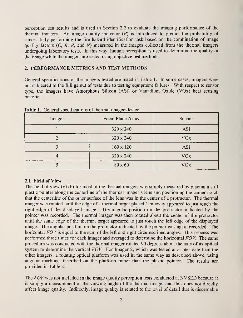
General specifications of the imagers tested are listed in Table 1 . In some cases, imagers were
not subjected to the full gamut of tests due to testing equipment failures. With respect to sensor
type, the imagers have Amorphous Silicon (ASi) or Vanadium Oxide (VOx) heat sensing
material.
Table 1. General specifications of thermal imagers tested.
Imager Focal Plane Array Sensor
1 320 X 240 ASi
2 320 X 240 VOx
3 160 X 120 ASi
4 320 X 240 VOx
5 80x60 VOx
2.1 Field of ViewThe field of view (FOV) for most of the thermal imagers was simply measured by placing a stiff
plastic pointer along the centerline of the thermal imager's lens and positioning the camera such
that the centerline of the outer surface of the lens was in the center of a protractor. The thermal
imager was rotated until the edge of a thermal target placed 1 m away appeared to just touch the
right edge of the displayed image. The angular position on the protractor indicated by the
pointer was recorded. The thermal imager was then rotated about the center of the protractor
until the same edge of the thermal target appeared to just touch the left edge of the displayed
image. The angular position on the protractor indicated by the pointer was again recorded. The
horizontal FOV is equal to the sum of the left and right circumscribed angles. This process wasperformed three times for each imager and averaged to determine the horizontal FOV. The same
procedure was conducted with the thermal imager rotated 90 degrees about the axis of its optical
system to determine the vertical FOV. For Imager 2, which was tested at a later date than the
other imagers, a rotating optical platform was used in the same way as described above, using
angular markings inscribed on the platform rather than the plastic pointer. The results are
provided in Table 2.
The FOV was not included in the image quality perception tests conducted at NVSED because it
is simply a measurement of the viewing angle of the thermal imager and thus does not directly
affect image quality. Indirectly, image quality is related to the level of detail that is discemable

within the field of view, and this is captured by measuring spatial resolution, which is an
important factor in image quality and is measured in both the laboratory tests and the humanperception tests. Also, the FOV does affect firefighter performance in that a narrower (versus
Table 2. Horizontal and vertical FOF results.
Imager Vertical FOF (degrees) Horizontal FOK (degrees) Aspect Ratio
1 33 ±0.6 42.5 ± 0.6 0.78 to 1
2 28 ± 0.6 33.5 ±0.6 0.84 to 1
3 33 ± 0.6 42.5 ±0.6 0.78 to 1
4 32 ±0.6 43.0 ±0.6 0.74 to 1
5 19 ±0.6 24.0 ±0.6 0.79 to 1
The uncertainty expressed in these test measurements is a combination of Type A (statistical)
and Type B (other), with a coverage factor of 2 resulting in a 95 % confidence interval. See
Section 5 for detailed uncertainty analysis.
wider) FOV limits the situational awareness of a firefighter that uses the imager to scan or
navigate a smoke-filled room.
The information provided in Table 2 shows that the design of thermal imager optical systems
varies significantly, even in cases where the same sensing material and detector array size are
used. The percent difference in average (combined vertical and horizontal) FOK between Imager
1 and Imager 5 is 75 %.
2.2 Nonuniformity
Nonuniformity (NU) is a measure of the thermal imager's response to a uniform thermal target [2,
3]. A common malady of thermal imaging is the phenomenon whereby the individual
subcomponents (pixels) of the thermal detector drift away from their initial values over time due
to minor variations in the sensing material and electronic circuitry. To compensate for this drift,
some types of imagers employ a shutter that closes over the detector and momentarily blocks
incoming radiation, effectively resetting all the pixels to the ambient temperature of the shutter.
The shutter is activated according to proprietary algorithms; this process is termed a
nonuniformity correction (NUC).
Three tests for each thermal imager were conducted at each of five target temperatures: 1 °C,
30 °C, 100 °C, 160 °C, and 260 °C, which span the temperature range of interest to the fire
service [4]. Well-characterized extended-area blackbodies were used as targets (a CI Systems
SR800 was used for target temperatures below 260 °C and a CI Systems SR80-HT was used for
the 260 °C target temperature). The thermal imager under test was positioned such that the
image of the blackbody surface completely filled the field of view and the thermal imager was
normal to the plane of the blackbody surface.
A Nikon D3 digital visible camera was used to take ten 16-bit digital photos of the images
displayed by the thermal imager under test for each target temperature. These images were

initially stored in flash memory on the Nikon, and then transferred to a PC for further processing.
The processing steps were as follows:
1. Convert the images from the proprietary Nikon NEF format to 16-bit TIFF files.
2. Convert the TIFF files to grayscale as defined per lEC 61966-2-1 (1999) [5].
3. Use a MATLAB program to define a region of interest (ROI) that encompasses at least
90 % of the FOV of the thermal imager under test. Exclude or remove symbols, icons,
and text fi-om this ROI.
4. Filter out the high-frequency noise created by oversampling the thermal imager's display.
This was accomplished with an averaging filter which averaged over an area whose width
and height was determined by the frequency of the noise.
5. Calculate the NU for each image using the following equation [3]
NU ^ (1)
Where a is the standard deviation and /u is the mean, respectively, of pixel intensity
values in the ROI. Retain the original pixel intensity values for later use.
6. Rank the ten NU values collected at each target temperature, then discard the highest NUvalue from the data set. This step is performed to mitigate the affect of an ill-timed NUCthat may occur during the collection of images.
7. Average the NU values for the three individual tests conducted at each target temperature.
This is the A^ value reported for each target temperature in Table 3.
The accuracy of the temperature measurements described in this section is discussed in Section 5,
uncertainty analysis.
Table 3. vVL^ values for a range of set point temperatures.
Imager NU\ °C iV;730°C NU\00°C NU \60°C NU260°C
1 0.324 ±0.019 0.497 ± 0.049 0.619 ±0.021 0.471 ±0.010 0.161 ±0.100
2 0.457 ± 0.023 0.360 ± 0.046 0.281 ±0.013 0.296 ±0.005 0.235 ± 0.022
3 0.395 ±0.145 0.393 ± 0.043 0.544 ± 0.007 0.702 ± 0.038 0.665 ±0.013
4 0.524 ±0.042 0.355 ± 0.096 0.617 ±0.024 0.172 ±0.016 0.761 ±0.038
5 0.239 ±0.007 0.339 ±0.004 0.397 ±0.032 0.404 ±0.214 0.349 ± 0.006
The uncert
and Type I
Secfion 5 f
ainty expressed in these test measurements is a combination of Type A (statistical)
^ (other), with a coverage factor of 2 resulting in a 95 % confidence interval. See
or detailed uncertainty analysis.

Imager 1 Imager 3 Imager 4 Imager 5
Figure 1. Representative images used for laboratory measurements of nonuniformity. The target
temperature is 100 °C.
A representative image from each of the thermal imagers, taken at the target temperature of
100 °C is shown in Figure 1. Note that these images have been modified to remove identifying
symbols and icons that would normally reside within the displayed imaged.
2.3 Spatial Resolution
The spatial resolution (SR) performance metric is a measure of the ability of firefighter thermal
imagers to reproduce the details of a scene or target [6]. The spatial resolution test is used both
to measure an imager's spatial resolution and to determine whether a design robustness test, e.g.,
the corrosion resistance test, has impacted the imager's ability to produce images of acceptable
quality.
This test was performed three times for each imager and the results were averaged to determine
the SR. Similar to the nonuniformity test, the SR was measured by viewing an image on the
thermal imager's display with a high resolution digital visible camera. The thermal imager
viewed a thermal target comprised of two sets of converging lines, as shown in Figure 2. This
target is a portion of the target used by the ISO Spatial Resolution Standard ISO 12233 [7]. The
target foreground and background were coated with well-characterized black paint having an
emissivity of 0.94 ± 0.05. The characterization of the black paint was performed by the paint
manufacturer.
Figure 2. Spatial resolution thermal target. The foreground (black markings) is held at a
constant temperature of 3 °C above ambient. The target size is 61 cm measured along the
centerline of each of the two converging line sets.

The thermal imager under test was placed 1 m from the target, normal to the plane of the target,
and oriented to focus on the center of the target. A Nikon D3 digital visible camera was used to
take ten 1 6-bit digital photos of the images displayed by the thermal imager under test, as shown
in the left image in Figure 3. These images were initially stored in flash memory on the Nikon,
then transferred to a personal computer (PC) for further processing. The processing steps were
as follows:
1
.
Convert the images from the proprietary Nikon NEF format to 1 6-bit TIFF files.
2. Convert the TIFF files to grayscale as defined per lEC 6 1 966-2- 1 ( 1 999) [5]
.
3. Filter out the high-frequency noise created by oversampling the thermal imager's display.
This was accomplished with an averaging filter which averaged over an area whose width
and height was determined by the frequency of the noise.
4. Use a MATLAB program to rotate the image 45 degrees and select an ROI that
encompasses the converging lines, as shown in the right image in Figure 3, and calculate
the contrast transfer function (CTF) at least at each of the index numbers along the two
sets of converging lines; a process that calculates the CTF at each row in the ROI is also
acceptable. The CTF is calculated using the following equation:
f^'TfP _ max min
max min
(2)
where I^ax and In,i„ are the highest and lowest pixel intensity values, respectively, along a
row of pixels cut through the pattern at least at each index line as indicated by the dotted
lines in the right image in Figure 3. Retain the original pixel intensity values for later use.
Pixels that represent symbols, icons, or text are excluded from the analysis.
5. The CTF values are multiplied by 7r/4 and paired with the frequencies of each index
number to construct a Modulation Transfer Function (MTF) curve. The frequencies are
listed in Table 4 below.
Table 4. Frequencies corresponding to the indices on the spatial resolution target when the
thermal imager under test is placed 1 m from the target.
Index Frequency (cycles/mrad)
1 (largest end of lines) 0.019
2 0.038
3 0.083
4 0.118
5 0.143
6 0.167
7 0.200
8 0.250
9 0.286
10 (smallest end of lines) 0.300

6. The MTF curve is normalized to the value obtained at the low-frequency edge of the
target (index 1).
7. The average NU value measured at a target temperature of 30 °C, and listed in Table 3, is
subtracted from the KfTF curve. This adjustment corrects for the effects of high
frequency noise.
8. The area under the normalized and adjusted MTF curve is the spatial resolution.
Figure 3. Spatial resolution image on left with a dashed box indicating the inset image on right.
The ROI is between the solid white lines in the right image and the dotted lines show the position
and orientation of the rows of pixels used to calculate the CTF.
The accuracy of the temperature measurements described in this section is discussed in Section 5,
uncertainty analysis.

Table 5. Spatial resolution test results.
Imager SR
1 0.0442 ± 0.0039
2 0.0389 ± 0.0043
3 0.0305 ± 0.0008
4 0.0402 ± 0.0089
5 0.0445 ±0.0013
The uncertainty expressed in these test measurements is a combination of Type A (statistical)
and Type B (other), with a coverage factor of 2 resulting in a 95 % confidence interval. See
Section 5 for detailed uncertainty analysis.
2.4 Effective Temperature RangeThe Effective Temperature Range (ETR) test measures the ability of a firefighter thermal imager
to see relatively small temperature differences in cases when large temperature differences exist
in the field of view [1]. In this test, the thermal imager is positioned such that it views a set of
contrast bars having constant temperature while the temperature of a surface of equal size in the
field of view is increased from near ambient to 550 °C. In general, as the hot surface
temperature increases, the contrast of the bars decreases. This test, as described in Draft NFPA1801, also has a color component in which the colorization corresponding to certain surface
temperature ranges is verified. The colorization employed by the imagers tested for this workwas not designed to conform with Draft NFPA 1801, therefore the color component of this test is
not reported here.
The thermal imagers were placed 1 m from the bar target, which were comprised of four vertical
1.27 cm diameter copper tubes placed 1.27 cm apart, resulting in a bar frequency of 0.04
cycles/mrad. A heated siloxane solution flowed through the bars to maintain a temperature of
37 °C ± 1 °C. The background temperature was 28 °C ± 1 °C. The bars and background were
coated with black paint having an emissivity of 0.94 ± 0.05. A CI Systems SR80-HT extended
area blackbody having a 178 mm square surface was positioned such that its radiation impinged
on a 203 mm diameter off-axis parabolic mirror having a focal length of 1 m and an offset of 1
degrees and was directed to the thermal imager under test. The layout of the testing equipment is
shown in Figure 4. It is important that the emitting surface of the blackbody appear in the center
of the image displayed by the thermal imager, while the heated bars appear at one side.
The size of the blackbody radiation in the thermal imager's field of view was at least as large as
the bars, but varied depending on the field of view of the thermal imager under test. A Nikon D3digital visible camera was used to take 16-bit digital photos of the image displayed by the
thermal imager every 3 seconds. These images were initially stored in flash memory on the
Nikon, then transferred to a PC for further processing. The processing steps were as follows:
1 . Convert the images from the proprietary Nikon NEF format to 16-bit TIFF files.

2. Convert the TIFF files to grayscale as defined per International Electrotechnical
Commission (lEC) 61966-2-1 (1999) [5].
3. Filter out the high-frequency noise created by oversampling the thermal imager's display.
This was accomplished with an averaging filter which averaged over an area whose width
and height was determined by the fi-equency of the noise.
4. Use a MATLAB program to define an ROI that encompasses the four vertical bars.
Exclude or remove symbols, icons, and text from this ROI. Retain the original pixel
intensity values for later use.
5. Use the MATLAB program to calculate the CTF of the bars within the ROI. The CTF is
calculated using equation 2.
6. The ETR is the temperature at which the CTF of the bars falls below a predetermined
value. The cut-off value is not specified for this test in lieu of the image quality indicator
discussed in Secfion 2.2.
The ETR data is plotted and discussed in Section 3.4 in the context of the image quality indicator.
Parabolic Mirror:
Focal length 1.0 mOff axis distance 0.176 mOff axis angle 10°
Clear aperture 0.2 m
Heated bars
O O O O
178 nnm square
extended area~ blackbody"
3-CD—
%
39L
30}CD
Figure 4. ETR testing configuration. The target consists of the heated bars, which appear on
the side of the image, and the emitdng surface of the blackbody, which appears in the center
of the image.
9

2.5 Thermal Sensitivity
The thermal sensitivity (TS) test measures the abihty of fire fighting thermal imagers to discern
small temperature differences [1]. Three tests for each thermal imager were conducted at each of
five target temperatures: 1 °C, 30 °C, 100 °C, 160 °C, and 260 °C, which span the temperature
range of interest to the fire service [4]. In most cases, a pair of well-characterized extended area
blackbodies were used as targets. A CI Systems SR800 was used for target temperatures
between 1 °C and 160 °C, which is the temperature range of this blackbody, a CI Systems SR80-
HT was used for target temperatures above 30 °C since this blackbody cannot be cooled below
30 °C, and an IRCon BCN-07C cavity blackbody combined with a 20.3 cm diameter spherical
mirror having a focal length of 30.5 cm was used for the 260 °C target temperature because the
SR800 could not produce this temperature. A metal 3.8 liter (1 gallon) container coated with
black paint having an emissivity of 0.94 ± 0.05 filled with ice water was used for the 1 °C target
temperature because only the SR800 could be cooled below ambient temperatures. The thermal
imager under test was positioned such that the image of two blackbody surfaces equally filled as
much of the field of view as possible. The amount of the field of view filled by the blackbody
surfaces depended on the optical geometry of the thermal imager under test. The thermal imager
was positioned normal to the plane of the blackbody surfaces. The purpose of having two
blackbody surfaces in the field of view was to force the automatic gain control (AGC) function
of the imagers to stabilize during the test. A significant portion of a typical image used to
calculate TS consists of surfaces at ambient temperature, which also contributed to the
stabilization of the AGC.
For each nominal target temperature (T„) below 260 °C, one blackbody was held at a constant
temperature. The other blackbody was initially set at T„ - 0.05 °C and ten 16-bit digital photos
were collected from the thermal imager display with a Nikon D3 digital visible camera. The
blackbody was then set at T„ and ten more images were collected. The blackbody was then set at
T„ + 0.05 °C and ten more images were collected. For the 260 °C nominal target temperature, the
same process was performed except that the temperature differences were T„ ± 0.20 °C. This
entire process was conducted three times for each imager at each nominal target temperature.
The images were initially stored in flash memory on the Nikon, then transferred to a PC for
further processing. The processing steps were as follows:
1. Convert the images from the proprietary Nikon NEF format to 16-bit TIFF files.
2. Convert the TIFF files to grayscale as defined per lEC 61966-2-1 (1999) [5].
3. Use a MATLAB program to define an ROI that encompasses at least 90 % of the area in
the field of view representing the blackbody surface that is set at T„ ± 0.05 °C or T„ ±
0.20 °C. Exclude or remove symbols, icons, and text fi-om this ROI. The three images in
Figure 5 are examples of ROIs used for the TS test.
4. Filter out the high-frequency noise created by oversampling the thermal imager's display.
This was accomplished with an averaging filter which averaged over an area whose width
and height was determined by the frequency of the noise.
5. Calculate the mean pixel intensity (ju) of the ROI. Retain the original pixel intensity
values for later use.
10

Rank the ten // values collected at each target temperature, then discard the lowestfj.
value from the data set. This step is performed to mitigate the affect of an ill-timed NUCthat may occur during the collection of images.
Average the remaining ninefj.
values for each set of images collected at each nominal
target temperature, i.e., at r„ and 7; ± 0.05 °C or T„ ± 0.20 °C.
Calculate the contrast between the average pixel intensity at r„ and Tn - 0.05 °C or
0.20 °C. Record this value. Calculate the contrast between the average pixel intensity at
Tn and r„ + 0.05 °C or 0.20 °C. Record this value. Average the two contrast values.
Average the contrast values per step 8 above for the three individual tests conducted at
each target temperature. This is the thermal sensitivity value reported for each target
temperature in Table 6.
Table 6. T lermal sensitivity test results.
Imager TS\ °C r^30°C r^-ioo^c r^l60°C r>S260°C
1
0.0134 ±
0.0123
0.0029 ±
0.0012
0.0028 ±
0.0018
0.0042 ±0.0006
0.0096 ±
0.0010
20.0316 ±
0.0213
0.0070 ±
0.0029
0.0030 ±
0.0015
0.0021 ±
0.0011
0.0011 ±
0.0003
30.0096 ±
0.0047
0.0067 ±
0.0023
0.0020 ±
0.0009
0.0020 ±
0.0020
0.0092 ±
0.0107
40.0282 ±
0.0110
0.0042 ±
0.0007
0.0016 ±
0.0002
0.0041 ±
0.0015
0.0026 ±
0.0009
50.0237 ±
0.0183
0.0104 ±
0.0039
0.0039 ±
0.0027
0.0025 ±
0.0007
0.0063 ±
0.0012
The uncertainty expressed in these test measurements is a combination of Type A (statistical)
and Type B (other), with a coverage factor of 2 resulting in a 95 % confidence interval. See
Section 5 for detailed uncertainty analysis.
An example of the contrast obtained from a TS test is presented in Figure 5. Note that, while
there may be a discemable difference in the average pixel intensity of the three images, there
may not be enough of a difference to provide useful images for the user of the thermal imager.
The very low contrasts recorded for the TS tests may not be sufficient for firefighters to locate
fire hazards or perform other tasks, so additional tests examined the change in contrast as the
value used for r„ was increased. Three tests were conducted at each r„ value for one imager.
The results are shown in Figure 6 and will be discussed in Section 3.4 in the context of the image
quality indicator.
11

>!iSjfT!i?;ffrrr'!5»T»r5jj^t5t^t;tt!r*t?t*{»i^^
^':
Figure 5. Example test images for TS at a nominal target temperature of 100 °C. The image on
the left is of a 100.05 °C target, the image in the center is of a 100.00 °C target, and the image on
the right is of a 99.95 °C target. Note that these three images may appear to be identical whenviewed on a printed page.
0.10
0.09
0.08
0.07
0.06
tt 0.05mw4->
Co 0.04u
0.03
0.02
0.01
0.00
N rX
•
u
^
m 11 '1 1 1 1
— —
I
500 1000 1500 2000 2500 3000 3500
Tn (mK)
Figure 6. Contrast response to increasing values of T„ for the TS test. The nominal target
temperature was 100 °C. The uncertainty expressed in these test measurements is a combination
of Type A (statistical) and Type B (other), with a coverage factor of 2 resulting in a 95 %confidence interval. See Section 5 for detailed uncertainty analysis.
12

3. MULTIVARIATE ANALYSIS
In order to determine the minimum level of image quality that allows users to successfully
perform meaningful tasks, a set of perception tests were conducted using firefighters that use
thermal imagers on the job. The test subjects were asked to observe thermal images of scenes in
which a single potential fire hazard may or may not be present. The test subjects identified the
hazard by clicking on it or, if no hazard was present, the test subject clicked a "No Hazard"
button. The contrast (Q, brightness (B), spatial resolution (R), and noise (N) in the thermal
images were degraded in varying degrees such that the effect of each of these primary quality
factors on the ability of a firefighter to perform a task was quantified. These primary factors
were chosen based on their relevance to the tests presented in Sections 2.2 to 2.5, although there
is not a 1-to-l correspondence. The measurement of contrast is fiindamental to all the imaging
tests conducted for this report. Brightness is used as an indication of the relative temperature of
surfaces in the field of view. Broadband noise, manifested as nonuniformity, and spatial
resolution are directly related to the test methods described in Sections 2.2 and 2.3, respectively.
During the process of analyzing the perception test results, it became apparent that the above
four primary factors of image quality were too tightly dependent upon one another to adequately
describe the imaging performance of a thermal imager if used in separate, individual
performance tests such as those presented in Sections 2.2 to 2.5. For example, the interaction of
contrast with brightness has a much more profound effect on a firefighter's ability to successfully
identify a fire hazard than the additive effect of contrast plus brightness. In order to
accommodate the interactions between primary image quality factors without disturbing the test
methods previously discussed, a human perception model was developed that includes the four
primary factors, as measured by the test methods described in Sections 2.2 to 2.5, along with
two-way interactions between these factors and squared terms of these factors. The model is
presented in its most compact form in the following equation:
(3)
where P is the probability of successfijUy identifying the fire hazard, or absence of a fire hazard,
in an image. For the purposes of this report, P is the image quality indicator. The variable Xrepresents a long set of terms in the form
X = 0.2563 + C + B + R + N + C^ +B^ +R' +N' +CB + CR + CN + BR + BN + RN (4)
13

where C, B, R, and A'^ are the contrast, brightness, spatial resolution, and noise that were present
in the images observed by the firefighters during their perception tests. The coefficients assigned
to each of the terms in equation 4 are listed in Table 7 below.
Table 7. List of coefficients that apply to terms in equation 4.
Coefficient Teiin
0.2563 intercept
0.8737 C
0.4595 B
15.85 R
-2.567 N-8.359 d-4.631 B'
-242.2 R'
2.893 N'
3.779 CB
48.71 CR
11.60 CN
34.91 BR
-8.016 BN
-5.008 RN
Several methods were used to validate the model represented by this equation, which will be
discussed in depth in a future publication. One of the methods used is to plot the averaged data
collected in the perception tests for each of the 25 different image degradation settings against
values predicted by the model. This is done in Figure 7, which shows a very good correlation
between actual data and predicted values.
14

0.8-
iy"0.7
-
Model
Prediction
o
O
cn
o)
1
1
2gl'.'-'22
y'iA
0.4- y' 5
0.3- ,'
0.2-
1J9'''
1 1 ' 1 ' 1 ' I ' 1
0.2 0.3 0.4 0.5 0.6
Observed Result
0.7 0.8
Figure 7. A comparison of the observed and model predicted values for the probability of
successfully completing the fire hazard identification task. The plot character represents the
image setting (1 to 25). A perfect correlation falls at the 45° diagonal.
Finally, a consistency check was performed to observe the predicted values from the model as
each primary image quality factor was varied across the range of possible values, holding the
other factors constant at their average value. This is shown in Figure 8. Note that all the factors
vary from to 1 except R, which is plotted using the uppermost x-axis. Also, note that the model
is useful for predictions within the range of factor values that were used in the perception tests;
extrapolation beyond this range of values for each factor is less useful.
15

0.005
Spatial Resolution Value
0.01 0.015 0.02 0.025 0.03 0.035 0.04 0.045 0.05
m
c
re
are
E
0.9
0.8
0.7
0.6
0.5
0.4
0.3
± 0.2
0.1
1 11 1 1 ^ 1 i 1
^̂I^^^^==*""^5:<^^'''^'^^-'—^ ^^"^"'''^^
/^ —-^"^ ^ \v
^—^^^^^ ^\vP{N) P(C) ---riu; KiK)
r 1 1 1 1 1 1i
1
0.9
0.8
0.7
0.6
0.5
0.4
0.3
0.2
0.1
0.1 0.2 0.3 0.4 0.5 0.6 0.7 0.8 0.9
Primary Factor Value (excluding Spatial Resolution)
Figure 8. Plot of each image quality factor as it varies from to 1 (0 to 0.05 for R) while the
other factors are held constant at their average values.
In order to optimize the perception testing procedure and reduce test subject fatigue, the range of
values used for the primary image quality factors in the degraded images were chosen to explore
a particular region of the probability of successfully performing the fire hazard identification task,
this region was 0.6 < P < 0.9. The reasoning was that collecting data from images in which none
of the test subjects were able to identify anything did not yield valuable information for the
purposes of this work. Likewise, using images in which all test subjects were able to identify the
fire hazard would not provide useful information from which to construct the model. Therefore,
no images were degraded to "zero" values of any of the primary image quality factors. It should
be also noted that the upper end of the N primary factor was not within the range ofN values
used to construct the model and values above about 0.6 are extrapolated.
3.1 Nonuniformity and Spatial Resolution Procedure
The measurement of nonuniformity at the target temperature of 30 °C is independent of the
image quality equation and is performed strictly in conformance with the method described in
Section 2.2, in which the standard deviation of the pixel intensity is divided by the mean pixel
intensity of a ROI within an image. This is the only test that does not require the use of equation
3 and is used to establish the primary factor R. The nonuniformity tests conducted at target
temperatures of 1 °C, 100 °C, 160 °C, and 260 °C make use of equation 3 and therefore
16

necessitate a pre-existing value for R. This will become apparent as the procedure is explained
below.
1. For the target temperature of 30 °C, follow the A/^L'^ procedure outlined in Section 2.2.
2. Follow the procedure outlined in Section 2.3 to calculate the spatial resolution, SR. Toapply equation 3, use the contrast measured at the low-frequency edge of the spatial
resolution target as C, use the average pixel intensity within the spatial resolution ROI as
B, use the measured spatial resolution as R, and use the nonuniformity measured in step 1
above as A^.
3. Calculate the image quality indicator, P. If P indicates less than the desired image
quality level, then the imager fails the entire test sequence and no further testing is
necessary.
4. IfP indicates image quality that is greater than or equal to the desired level at the target
temperature of 30 °C, apply equation 3 to the nonuniformity data collected at target
temperatures of 1 °C, 100 °C, 160 °C, and 260 °C, applying equation 3 separately to data
collected at each target temperature. For these tests, use the same contrast value as in
step 2 for C, use the average pixel intensity within the nonuniformity ROI as B, use the
same measured spatial resolution as in step 2 for R, and use the nonuniformity measured
according to the procedure outlined in Section 2.2 at each of the target temperatures (1 °C,
100 °C, 160 °C, and 260 °C) as N.
5. Calculate the image quality indicator, P. If P indicates less than the desired image
quality level, then the imager fails the entire test sequence and no further testing is
necessary.
6. If P indicates image quality that is consistently greater than or equal to the desired level,
continue to the test sequence for effective temperature range in the following section.
3.2 Effective Temperature Range Procedure
The procedure for applying equation 3 to the data collected for the effective temperature range
test is relatively simple. For this test, the image quality indicator, P, is calculated using pixel
intensities from the ROI encompassing the bars for each image collected during the test. The
procedure is explained below.
1
.
Follow the ETR procedure outlined in Section 2.4.
2. To apply equation 3, use the CTF of the bars as the contrast C, use the average pixel
intensity of the bar ROI as the brightness B, use the same measured spatial resolution as
in step 2 of Section 3.1 for R, and use the nonuniformity value obtained at a target
temperature of 30 °C in step 1 of Section 3.1 as A^.
3. Calculate the image quality indicator, P, for each image collected during the test. If any
of the calculated values ofP indicate less than the desired image quality level, the imager
under test fails the entire test sequence and no further testing is necessary.
4. If P indicates image quality that is consistently greater than or equal to the desired level,
continue to the test sequence for thermal sensitivity in the following section.
17

3.3 Thermal Sensitivity Procedure
The procedure for applying equation 3 to the data collected for the thermal sensitivity test is also
relatively simple. For this test, the image quality indicator, P, is calculated using a contrast
measurement that depends on subtle changes in pixel intensity resulting from small changes in
the target surface temperature. The procedure is explained below.
1
.
Follow the TS procedure in Section 2.5.
2. To apply equation 3, for each nominal target temperature, use the contrast obtained in
step 9 of Section 2.5 as C, use the average pixel intensity of the bar ROI as the brightness
B, use the same measured spatial resolution as in step 2 of Section 3.1 for R, and use the
nonuniformity value obtained at the corresponding target temperature as A^.
3. Calculate the image quality indicator, P, at each nominal target temperature. If any of the
calculated values ofP indicate less than the desired image quality level, the imager under
test fails the entire test sequence and no further testing is necessary.
4. IfP indicates image quality that is consistently greater than or equal to the desired level,
the imager under test has successfully completed the sequence of image quality tests.
3.4 Multivariate Image Quality Results
The results shown in this section consider the same test conditions and data that were collected
using the test methods presented in Sections 2.2 to 2.5 but offer the added benefit of
incorporating the effects of interactions between the primary image quality factors. Using
equation 3 in this way allows the pass/fail criteria for the image quality test methods to be based
on human perception of images that relate to tasks performed in the user's line of duty.
3.4.1 Nonuniformity
The nonuniformity {NU) results, expressed in terms of the image quality indicator, P, are shownbelow in Figure 9. The mid-range target temperatures of 100 °C and 160 °C, at which some of
the imagers show a larger uncertainty, are in the vicinity of the mode-shift trigger for those
imagers. An automatic mode shift is a method used in thermal imagers that employ a
microbolometer type detector to extend the dynamic range of the imager by decreasing the
integration time that the thermal scene is exposed to the detector array. A side effect of
operating at the shorter integration time is reduced thermal sensitivity; this will be explained in
more detail in the thermal sensitivity discussion. The effect on the nonuniformity results
presented here is that the imager may automatically shift for one of the three tests conducted at
each target temperature, and not shift for the other two tests if the mode shift algorithm isn't
triggered. The mode shift algorithm is a proprietary process and can depend on many conditions
in the thermal scene, including but not limited to target temperature. This phenomenon can maketesting the imagers problematic if the target temperature and other conditions are very close to
the mode shift conditions.

1
0.9
0.8
0.7 i3 I
I "-5 i T•ac> 0.5
fO
3a 0.4
QibOre
E 0.3
X
0.2 -j
0.1
i
&
I
¥
Imager 1 X Imager 2 ^Imagers irimager 4 ©Imagers
50 100 150 200
Target Temperature (°C)
250 300
Figure 9. Nonuniformity (NU) plotted in terms of the image quality indicator, P. The
uncertainty expressed in these test measurements is a combination of Type A (statistical) and
Type B (other), with a coverage factor of 2 resulting in a 95 % confidence interval. See Section 5
for detailed uncertainty analysis.
3.4.2 Spatial Resolution
The spatial resolution (SR) results, expressed in terms of the image quality indicator, P, are
shown below in Figure 10. With the exception of imager 1, the imagers produced similar SRresults in spite of having different values of C, B, R, and N in equation 3.
19

Figure 10. Spatial resolution {SR) plotted in terms of the image quality indicator, P. The
uncertainty expressed in these test measurements is a combination of Type A (statistical) and
Type B (other), with a coverage factor of 2 resulting in a 95 % confidence interval. See Section 5
for detailed uncertainty analysis.
3.4.3 Effective Temperature Range
The effective temperature range (ETR) results for Imagers 3, 4, and 5, expressed in terms of the
image quality indicator, P, are shown below in Figures 11, 12, and 13, respectively. Three tests
were conducted for each imager. Technical difficulties with the blackbody used as the hot
surface prevented the collection of data for all imagers. Mode shifts can be observed as jumps in
the data near the same hot surface temperature for all three tests. Imagers 3 and 4 produced
higher P values after the mode shifts. Imager 5 did not display a pronounced mode shift.
20

1
0.9
0.8
sM 0.6
1f 0.5
T3
§ 0.4wuI 0.3
0.2
0.1
1TC3
!
1
!
1
d "
f
!
i
!
i 3'
! i ; 1 1 ! 1
50 100 150 200 250 300
Hot Surface Temperature TO
350 4CK» 450
Figure 11. Effective Temperature Range (£"77?) for Imager 3 plotted in terms of the image
quality indicator, P. Each colored line represents the results of one test.
21

1
0.9
0.8
0.7
rou 0.6XJC•">•4-' 0.5
TO3a 0.4(U00nj
£ U.3
0.2
0.1
TIC4
50 100 150 200 250 300
Hot Surface Temperature {°C)
350 400 450
Figure 12. Effective Temperature Range (ETR) for Imager 4 plotted in terms of the image
quality indicator, P. Each colored line represents the results of one test.
22

Figure 13. Effective Temperature Range {ETR) for Imager 5 plotted in terms of the image
quality indicator, P. Each colored line represents the results of one test.
3.4.4 Thermal Sensitivity
The thermal sensitivity {TS) results, expressed in terms of the image quality indicator, P, are
shown below in Figure 14. All the imagers appeared to perform best at the cool nominal
temperature of 1 °C. There is no significant trend in the test results at nominal target
temperatures above 1 °C. These chaotic results indicate the need to look more closely at the
temperature difference {T„) used in the test. Theoretically, if the imager's detector is the limiting
system component, the imager should show a decrease in P when operating in the low sensitivity
mode (shorter integration time), which is not apparent in Figure 14.
23

0.9
0.8
^- 0.7
On.y 0.6ac
"(5
a 0.4 -
<u
ns
£ 0.3
0.2
0.1
# Imager 1 X Imager 2 9 imager 3 _^_ Imager 4 ® Imager 5
«
1m
<A
i
X
f
^
50 100 150 200
Nominal Target Temperature (°C)
250 300
'. figure 14. Thermal Sensitivity {TS) plotted in terms of the image quality indicator, P. Theuncertainty expressed in these test measurements is a combination of Type A (statistical) and
Type B (other), with a coverage factor of 2 resulting in a 95 % confidence interval. See Section 5
for detailed uncertainty analysis.
There are several factors to consider when attempting to measure very fine differences in
temperature. First, the target temperature must be well characterized and measured with
sufficient accuracy. Second, the thermal sensitivity of the temperature sensing device under test
must be capable of resolving the temperature difference. Third, the displayed image must be
resolved with enough shades of gray to provide a contrast that can be perceived by the user.
The blackbody used to produce T„ in this test (CI Systems SR-800) has a temperature accuracy
of 8 mK for temperatures below 50 °C and 15 mK for temperatures above 50 °C, however, its
temperature range is restricted to °C to 175 °C. For the 260 °C test point, the CI Systems SR-
80-7HT has a temperature accuracy of 0.5 °C, although there are other commercially available
blackbodies that are more accurate at this temperature. If this test method was modified to
require thermocouple temperature measurements, the accuracy of these measurements falls to l.l
°C or 0.4 %, whichever is greater. A differential blackbody could be utilized, however, these
instruments are restricted to temperature differences near ambient temperature.
The thermal sensitivity of the imager's detector comes into play when the dominant temperature
difference in the imager's field of view is relatively small. For the nominal target temperature of
24

30 °C, the limiting component would be the detector if the user could discern individual levels of
grayscale.
The displays used for fire service thermal imagers have 8-bit grayscale resolution; therefore,
scenes in which temperature differences exist on the order of 250 °C could not be expected to be
resolved to less than in 1 °C increments. Following this logic, the smallest value of T„ that can
be resolved on the imager's display (one increment of grayscale) for each of the nominal target
temperatures, assuming an ambient temperature of 25 °C and a 50 mK detector thermal
sensitivity, is listed in Table 8.
'able 8. Minimum resolvable T„ due to imager component limitations.
Nominal Target Temperature (°C) Minimum T„ Limitation
1 94 mK display
30 50 mK detector
100 293 mK display
160 527 mK display
260 918 mK display
Given the minimum T„ values needed to produce one increment of grayscale on an 8-bit display
at the nominal target temperatures required in this test sequence, it is useful to examine the
response of the imager to increasing values of T„. This is done for one imager in Figure 15. The
data presented in Figure 1 5 shows that, when plotted in terms of P, holding all the other image
quality factors constant and increasing the T„ from 50 mK to 3000 mK, P remains quite low
while the uncertainty in the measurement increases substantially.
25

Figure 15. Thermal sensitivity as a function of increasing delta T {T„). The uncertainty
expressed in these test measurements is a combination of Type A (statistical) and Type B (other),
with a coverage factor of 2 resulting in a 95 % confidence interval. See Section 5 for detailed
uncertainty analysis.
In order to improve the application of this test to fire service thermal imagers, several options
may be considered. Possible changes to the test method are listed below, note that this is not an
exhaustive list.
1
.
Leave the test method as is.
2. Make this measurement only at one (ambient) nominal target temperature, using a
differential blackbody to measure the temperature difference.
3. Use the imager's detector thermal sensitivity specification, which is measured as the
NETD, as the imager's thermal sensitivity.
4. Adjust the T„ values as necessary to account for resolution limitations imposed by system
components.
5. Lower the acceptable image quality indicator value, P, to a value that does not eliminate
all the thermal imagers in the commercial fire service market.
6. As a last resort, remove this test method from the suite of image quality tests until a more
suitable test method is developed.
26

4. UNCERTAINTY ANALYSIS
There are different components of uncertainty in the measurements made with the equipment
used in the tests discussed in this report. Type A uncertainties are those which are evaluated
using statistical methods and Type B uncertainties are those which are estimated using other
means, such as experience with a particular type of equipment. Type B uncertainties are
evaluated by estimating the upper and lower limits for the quantity in question such that the
probability that the quantity would fall within the upper and lower limits is essentially 100 %.
After estimating the uncertainties by Type A and Type B analysis, the results are combined in
quadrature to yield the combined standard uncertainty. When the combined standard uncertainty
is multiplied by a coverage factor of two, the result is the expanded uncertainty which
correspond to a 95 % confidence interval (2a).
The components of uncertainty are listed in Table 9. Some of these components, such as the
blackbody temperature measurements, are derived from instrument specifications. Other
components, such as the angular FOV measurements, are estimated based on estimates of
uncertainty in reading the angular markings on the protractor or rotating platform.
Table 9. Components used in uncertainty analysis.
ComponentType A
UncertaintyType B Uncertainty
Combined
Uncertainty
Total
Expanded
Uncertainty
FOWangle a 0.25 degrees a + 0.25 degrees 0.6 degrees
SR-800
Blackbody
G, pixel
intensities in
ROI
T < 50 °C: ± 8 mKT>50°C:±15mK
a + 8mKa+15mK
2(a + 8 mK)2(a+15mK)
SR-80-7HT
Blackbody
a, pixel
intensities in
ROI± 0.5 °C a + 0.5 °C 2(a + 0.5 °C)
IRConBlackbody
a, pixel
intensities in
ROI
T<316°C:2°CT>316T:0.5%
a + 2°C
a + 0.5 %2(a + 2 °C)
2(a + 0.5 %)
Type J
thermocouplesa
Greater of 1.1 °C or
0.4 %a+l.l°Cora + 0.4 %
2(a+I.l°Cor
a + 0.4 %)
TypeKThermocouples
aGreater of 1.1 °C or
0.4 %a+l.l°Cora + 0.4 %
2(a+l.l°Cor
a + 0.4 %)
The error bars and measurement accuracies shown in the figures and tables, respectively, in this
report reflect values calculated using the uncertainties listed in Table 8 above.
5. CONCLUSIONS
Five thermal imagers were provided by fire service thermal imager manufacturers for evaluation
using test methods designed specifically to assess their image quality performance for fire
27

service applications. These tests were Field of View (FOV), Nonuniformity (NU), Spatial
Resolution (SR), Effective Temperature Range (ETR), and Thermal Sensitivity (TS).
The FOVtQSt results show that the design of thermal imager optical systems varies significantly,
even in cases where the same sensing material and detector array size are used. The combined
horizontal and vertical FOVs differed by approximately 75 % from the narrowest to the widest
FOF values.
The NU test results, when considered in the context of human perception using the image quality
indicator (P), were generally reproducible and showed that all the imagers performed in the
range of about 0.6 to 0.95 across the set of five target temperatures. The uncertainty in these
measurements was larger for the 100 °C and 160 °C target temperatures, which is consistent with
observations that some of the imagers shifted sensitivity mode for one or two of the three tests
performed at these intermediate target temperatures.
The ETR tests show that, after an initial increase from ambient temperature, the three imagers
tested gave three distinctly different responses. Imager 3 has a higher value after the mode shift,
imager 4's performance didn't change noticeably due to mode shifts and was consistently higher
than the other two imagers, and the performance of imager 5 slowly decreased and then reached
a plateau with no indication of a mode shift.
The results of the TS tests are problematic. As the nominal target temperature increases above 1
°C, the performance of the imagers drops drastically and then becomes erratic at target
temperature above 100 °C. Part of the erratic nature of the data collected at higher temperatures
is due to the mode shift, for the same reason noted in the NU discussion above. This test does
not appear to fully capture the actual thermal sensitivity of the imager. A closer examination of
the response of two imagers to increasing the temperature difference {T„) used in this test showed
that the imagers don't discriminate significantly between a T„ of 50 mK and a T„ of 2000 mk.
28

References
[1] Amon, F., et al., Performance Metricsfor Fire Fighting Thermal Imaging Cameras -
Small- and Full-Scale Experiments . 2008
[2] Hoist, G.C., Testing and Evaluation ofInfrared Imaging Systems. 1998, Winter Park, FL:
JCD Publishing.
[3] Lock, A. and F. Amon. Measurement ofthe Nonuniformity ofFirst Responder Thermal
Imaging Cameras, in SPIE Defense + Security. 2008. Orlando, FL: SPIE.
[4] Donnelly, M.K., et al.. Thermal Environmentfor Electronic Equipment used by First
Responders. 2006(NIST Technical Note 1474).
[5] lEC, Multimedia systems and equipment - Colour measurement and management
International Electrotechnical Commission, 1999. lEC 61966-2-1.
[6] Lock, A. and F. Amon. Application ofSpatial Frequency Response as a Criterionfor
Evaluating Thermal Imaging Camera Performance, in SPIE Defense and Security
Conference. 2008. Orlando, Florida: SPIE.
[7] ISO, Photography - Electronic still-picture cameras - Resolution measurements.
International Standards Organization 2000. ISO 12233.
29

6. APPENDIX - EQUIPMENT LIST
Certain commercial entities, equipment, or materials may be identified in this document in order
to describe an experimental procedure or concept adequately. Such identification is not intended
to imply recommendation or endorsement by the National Institute of Standards and Technology,
nor is it intended to imply that the entities, materials, or equipment are necessarily the best
available for the purpose. When possible, readily available equipment that had already been
purchased for different tasks was utilized rather than purchasing new equipment that might be
better suited for the specific tasks in this project.
1 . Nikon D3 digital SLR camera.
http://www.nikonusa.com/Find-Your-Nikon/ProductDetail.page7pid-25434
Remote control cord.
http://www.nikonusa.com/Find-Your-Nikon/Product/Remote-Cords/4652/MC-22-
Remote-Cord-with-Banana-Plugs.html
Nikkor 28 mm lens.
http://www.nikonusa.com/Find-Your-Nikon/Product/Camera-Lenses/1922/AF-NIKKOR-
28mm-f%252F2.8D.html
+10 close-up filter.
http://www.bhphotovideo.com/c/product/94232-
REG/Hova_S52MCU 52mm Macro Close up 10 .html
Image conversion software (apparently the newest Photoshop CS4 includes the plug-in
necessary for use with Nikon D3 files).
http://bibblelabs.com/ or http://www.adobe.com/products/photoshop/cameraraw.html
Memory.
http://www.newegg.com/Product/Product.aspx?Item^N82E 168202 11244
Camera stand.
http://www.bhphotovideo.com/bnh/controller/home?ci=0&shs=^Manfrotto+by+Bogen+I
maging+SALON+230+CAMERA+STAND+(7%27)+-+BO809&sb=ps&pn=l&sq=desc&InitialSearch=yes&O=jsp%2Fcatalog.isp&A^search
&Q=*&bhs=t&Go.x=0«S:Go.v-0&Go-submit
Articulated camera positioning arm.
http://www.bhphotovideo.com/bnh/controller/home?0=search&A~search&Q=&shs=ma
nfrotto+by+bogen+imaging+articulated+ami+bracket+bo396b3&ci=0
Grip kit for the articulating arm.
http://www.bhphotovideo.com/bnh/controller/home?ci=0&shs=Avenger+GRIP+KIT%3
A+C 1 575B%2FD200B%2FE600%2FD520B%2FBAG+-+AVD800KIT&sb=ps&pn=l&sq=desc&InitialSearch=ves&O=isp%2Fproductlist.isp&A
=search&Q=*&bhs=t&Go.x=24&Go.v= 1 1&Go=submit
2. Data Acquisition System.
Controller card.
http://sine.ni.eom/nips/cds/view/p/lang/en/nid/14235
30

Chassis.
http://sine.ni.eom/nips/cds/view/p/lang/en/nid/10676
Analog In module, terminal block, and cable (use TC-2095 terminal).
http://sine.ni.eom/nips/cds/view/p/lang/en/nid/1654
http://sine.ni.eom/nips/cds/view/p/lang/en/nid/1676
http://sine.ni.eom/nips/cds/view/p/lang/en/nid/1834
Analog Out module and terminal block. This is to control relays that control the Nikon
D3 camera.
http://sine.ni.eom/nips/cds/view/p/lang/en/nid/1870
http://sine.ni.eom/nips/cds/view/p/lang/en/nid/1682
3. Emissivity paint.
Optical black coating, P/N 20825, Medtherm Corp., P. O. Box 412, Huntsville, AL.
Average emissivity = 0.95, ± 0.03.
4. Thermocouples.
Use Type-J thermocouples.
http://www.omega.com/pptst/SAl .html
5. Spatial resolution target.
See files: ImRecTarget.svg, ImRecTarget.eps, ImRecTarget.ai. Note- these are all the
same image but with different file formats.
The 24" X 36" siHcone rubber heating blanket for the background comes from:
http://www.briskheat.com/p-347-srl-srp-silicone-mbber-heating-blankets.aspx (use a
variac to control the temperature)
Metal target stencil.
Frederick Sign and Banner, 18 East 6"" St., Frederick, MD 21701, 301-663-9122.
6. Blackbodies.
One extended area blackbody that can go as low as °C, such as one of these:
http://www.ci-svstems.com/htmls/article.aspx7C2004-12724&BSP= 12547 (4", extended
temperature range).
http://www.sbir.conVblackbodv 1 3 1 32.htm (4", -30 to 100 °C temperature range)
http://www.mikroninfrared.com/Catalog.aspx7id-l 164&ekmensel-c580fa7b 8 28 1150
(4", -5 to 170 °C temperature range)
http://vyww.electro-optical.com/html/datashts/extended/pdf/eo710ces200.pdf
(4", note: temperature accuracy might be out of specification for NFPA 1801)
In all the above cases, the nonuniformity of the blackbody as measured in paragraph
8.1.5.13 needs to be verified.
A high temperature extended area blackbody.
http://www.ci-svstems.com/Htmls/article.aspx7C2004=12726«feBSP=12547
(Temperature range 30 °C to 550 °C)
http://vyw^.sbir.com/blackbodv 4000.htm
31

(Temperature range 30 °C to 550 °C)
http://www.mikroninfrared.corn/Catalog.aspx?id=2392&ekriiensel=c580fa7b_8_28_1150
_2
http://www.electro-optical.com/html/datashts/extended/pdf/CES600800RevisedC.pdf
(Temperature range 30 °C to 550 °C)
Effective Temperature Range Bars.
4 bars: 1.3 cm (V2 in) thick and set 1.3 cm (Yi in) apart; they are 15.2 cm (6 in) long.
They must maintain a constant temperature of 30 °C ± 0.5 °C. Suggestion: use
thermoelectric (peltier) heaters with a variac to control them.
32

