evaluation of precipitation over the middle east and

Evaluation of precipitation over theMiddle East and Mediterranean in

high resolution climate models

University of Reading

Department of Mathematics, Meteorology and Physics

David MacLeod

August 2009

Supervisors: Dr. Len Shaffrey and Dr. Emily Black

Submitted in partial fulfilment of the requirements for the degree of

MSc in Mathematical and Numerical Modelling of the Atmosphere and Oceans

Abstract

The Middle East is considered the worlds most water scarce region (Brown

& Crawford (2009)). In this study two high resolution climate models have

been evaluated to compare how successfully they model precipitation over

the region. One model is HiGEM (Shaffrey et al. (2009)), a global coupled

ocean-atmosphere model which operates at a resolution of 1.25◦ x 0.83◦ in

longitude and latitude for the atmosphere, and 1/3◦ x 1/3◦ in the ocean. The

other model is an atmosphre only regional model operating at a resolution

of 0.44◦ x 0.44◦ (Black (2009)).

It has been found that both models capture well the seasonal cycle of pre-

cipitation well, although the regional model underestimates the total amount.

10m surface wind fields and mean sea level pressure climatologies from the

models also have been compared with ERA-40 reanalysis data to investigate

the climatic processes represented in the models. It has been found that the

Cyprus low is not represented well in the regional model. The Cyprus low is

associated with eastward moving weather systems bringing most precipita-

tion to the region - an underestimation of the intensity in the regional model

is likely associated with underestimation of precipitation. It has also been

found that the regional model underestimates low level convergence in the

main region of precipitation and HiGEM overestimates it - likely to be as-

sociated with the underestimation and slight overestimation of precipitation

in this region in each of the models .

iii

iv Abstract

Two regions have been defined for statistical analysis and bias, root

mean square error and pattern correlations have been calculated for each.

The effect of smoothing precipitation fields on statistics has been investi-

gated. This investigation has been furthered by calculating fractions skill

score curves, a novel method implemented recently for numerical weather

prediction (Roberts & Lean (2008)). This method is new for climate anal-

ysis and comments on the usefulness of the method have been made, along

with recommendations for future use.

Acknowledgements

There are many people that I owe a debt of gratitude to academically and

non-academically - too many to name here. Thanks go to Len and Emily,

who gave me everything I needed from my supervisors, and more.

Thanks go to my parents - Dad for showing me that nothing is broken

which can’t be fixed, and Mum for reminding me what’s important when my

head gets filled up with big ideas.

I gratefully acknowledge NERC for their financial support, without which

I would have been unable to undertake this course.

Last but not least I thank my coursemates at Reading, who have been a

big part in making this year one of my best so far. Writing this dissertation

was (almost) a breeze with the company in room 105. Having others to share

the tea-making burden with helped me get through some of the harder bits

- sorry if I drank more than I made!

v

vi Acknowledgements

To those who do not know mathematics it is difficult to get across a real

feeling as to the beauty, the deepest beauty, of nature ... If you want to learn

about nature, to appreciate nature, it is necessary to understand the

language that she speaks in. - Richard Feynman

Acknowledgements vii

I confirm that this is my own work and the use of all material from other

sources has been properly and fully acknowledged.

· · · · · · · · · · · · · · · · · · · · · · · · · · · · · ·

· · · · · · · · · · · · · · · · · ·

List of Figures

1.1 Map of the Middle East . . . . . . . . . . . . . . . . . . . . . 2

1.2 IPCC predictions for climate change in the Middle East . . . . 6

2.1 Topography of the Middle East with HiGEM and RCM rep-

resentations of topography. . . . . . . . . . . . . . . . . . . . . 14

2.2 The domain over which the regional model is evaluated. . . . . 17

3.1 Precipitation observations from GPCC, GPCP and TRMM. . 22

3.2 Modelled precipitation fields for HiGEM and the RCM. . . . . 24

3.3 Mean sea level pressure climatologies from ERA-40 reanalysis,

HiGEM and the RCM. . . . . . . . . . . . . . . . . . . . . . . 26

3.4 Wind fields from ERA-40 reanalysis, HiGEM and the RCM. . 29

3.5 Errors in wind fields, calculated from differences between ERA-

40 and HiGEM and the RCM respectively. . . . . . . . . . . . 30

4.1 Examples of binary fields. . . . . . . . . . . . . . . . . . . . . 35

4.2 Idealised FSS curve . . . . . . . . . . . . . . . . . . . . . . . . 38

viii

LIST OF FIGURES ix

5.1 Map showing North and South regions, with a schematic show-

ing increasing sizes of smoothing boxes used for calculating

FSS curves. . . . . . . . . . . . . . . . . . . . . . . . . . . . . 40

5.2 FSS curves for the North region. . . . . . . . . . . . . . . . . . 46

5.3 FSS curves for the South region. . . . . . . . . . . . . . . . . . 47

Contents

Abstract iii

Acknowledgements v

List of figures ix

1 The Middle East 1

1.1 Geography . . . . . . . . . . . . . . . . . . . . . . . . . . . . . 2

1.2 Climate . . . . . . . . . . . . . . . . . . . . . . . . . . . . . . 3

1.3 Climate change predictions . . . . . . . . . . . . . . . . . . . . 5

1.4 Aims of the study . . . . . . . . . . . . . . . . . . . . . . . . . 8

2 Model description and observations 10

2.1 Climate Modelling . . . . . . . . . . . . . . . . . . . . . . . . 11

2.1.1 Model Resolution . . . . . . . . . . . . . . . . . . . . . 12

2.2 Description of models . . . . . . . . . . . . . . . . . . . . . . . 13

2.2.1 HiGEM . . . . . . . . . . . . . . . . . . . . . . . . . . 13

2.2.2 The Regional Climate Model . . . . . . . . . . . . . . . 16

x

CONTENTS xi

2.3 Description of observations . . . . . . . . . . . . . . . . . . . . 17

3 Visual comparison of climatologies 19

3.1 Precipitation . . . . . . . . . . . . . . . . . . . . . . . . . . . 20

3.1.1 Comparing observations . . . . . . . . . . . . . . . . . 20

3.1.2 Looking at the models . . . . . . . . . . . . . . . . . . 21

3.2 Mean Sea Level Pressure . . . . . . . . . . . . . . . . . . . . . 23

3.3 Surface Wind Patterns . . . . . . . . . . . . . . . . . . . . . . 27

3.3.1 Observed Wind Fields . . . . . . . . . . . . . . . . . . 27

3.3.2 Modelled Wind Fields . . . . . . . . . . . . . . . . . . 28

3.4 Discussion . . . . . . . . . . . . . . . . . . . . . . . . . . . . . 31

4 Statistical verification methods 32

4.1 Statistical measures of model skill . . . . . . . . . . . . . . . . 32

4.2 Fractions Skill Scores . . . . . . . . . . . . . . . . . . . . . . . 33

4.2.1 Conversion to binary fields . . . . . . . . . . . . . . . . 34

4.2.2 Generation of fractions . . . . . . . . . . . . . . . . . . 34

4.2.3 Computing fractions skill scores . . . . . . . . . . . . . 37

5 Statistics of model output 39

5.1 Standard model skill scores . . . . . . . . . . . . . . . . . . . . 39

5.2 Fractions Skill Scores. . . . . . . . . . . . . . . . . . . . . . . 43

6 Discussion and Conclusions 48

6.1 Model Evaluation . . . . . . . . . . . . . . . . . . . . . . . . . 49

6.2 FSS skill scores . . . . . . . . . . . . . . . . . . . . . . . . . . 50

xii CONTENTS

6.3 Future Work . . . . . . . . . . . . . . . . . . . . . . . . . . . . 52

References 55

Chapter 1

The Middle East

The Middle East is considered the world’s most water-scarce region (Brown

& Crawford (2009)). Water availability is important for human health and

economic activity and in many places demand for water already outstrips

supply. Current climate models predict that in the future the region will

experience a decrease in precipitation leading to a decrease in river runoff in

the region (Evans (2008), Kitoh et al. (2008)). Whilst models agree on the

direction of the changes in the water cycle, they do not agree on the mag-

nitude of these changes (Milly et al. (2005)). This may be partly because

the region has a sharp spatial gradient in climate types as well as a highly

varied landscape. The landscape and the climate interact in a complex way

which makes modeling future climate in the region a challenge for climate

models (Evans (2004)). One potential way of improving the skill of climate

predictions in the region is to increase model resolution, which gives advan-

tages such as better representation of weather systems and more accurate

topography. The effect of model resolution on representation of climate is

a main focus of this study. In this chapter the geography and the climate

of the region are discussed, along with current model predictions for future

climate of the region. The questions relating to modeling the climate of the

1

2 CHAPTER 1. THE MIDDLE EAST

region which will be addressed in this study are also set out.

1.1 Geography

A map of the Middle East is shown in figure 1.1. The region has a varied

landscape, from the Taurus mountains in Turkey and the Zagros mountains in

Iran to the deserts of Syria, Iraq, Jordan and Saudi Arabia. Surrounding the

region are several large bodies of water, moving clockwise from the eastern

coast of the Mediterranean; the Black Sea, the Caspian Sea, the Persian Gulf

and the Red sea.

Figure 1.1: A map of the Middle East, modified from GoogleEarth (2009)

Three main rivers run through the region and provide water to many

communities. The River Jordan is fed by tributaries from the countries sur-

rounding northern Israel and travels southwards along the boundary between

the West Bank and Jordan to the Dead sea. 70–90% of the water in the Jor-

1.2. CLIMATE 3

dan is used for human purposes, which has caused a large reduction in flow

of the river. Coupled with the high evaporation rate, this means that the

Dead sea is drying up (Klein & Flohn (1987)).

The two other major rivers in the region are the Tigris and the Eu-

phrates, which descend from the slopes of the Taurus mountains in Turkey

into Syria and Iraq before discharging into the Persian Gulf. These rivers de-

fine Mesopotamia, also known as the ”‘Cradle of Civilization’. This area saw

the development of some of the earliest human civilizations, in no small part

due to its rich, fertile soils – hence the name ‘The Fertile Crescent’. It has

now all but dried up, with much of the land cover transformed into bare land

and salt crust, and it is on the WWF list of critical/endangered ecoregions

(Olson & Dinerstein (2002)). Human activity is a major factor behind this

degradation – water diversion for agricultural irrigation and construction of

many dams in the headwaters of the Tigris and Euphrates have caused a

reduction in their annual flow (Partow (2001)). This combination of stress

on a fresh water source and rapid population growth substantially increases

the vulnerability of the region to future climate change (Evans (2008)).

1.2 Climate

The Middle East has a Mediterranean macroclimate, characterized by cool,

wet winters and hot, dry summers. Nearly all precipitation falls in winter,

the dominant mechanism being eastward moving cyclones from the Mediter-

ranean. The locations of precipitation are strongly influenced by surrounding

mountains (Smith et al. (n.d.)). There are five dominant regions of precipi-

tation associated with mountain ranges;

• The Mediterannean coastal range including the hills of Lebanon.

• The Taurus mountains of Turkey.


• The Zagros mountains of Iran.

• The Pontic range by the Black Sea.

• The Elburz range by the Caspian Sea.

Precipitation patterns are also influenced by the location of water bodies

adjacent to the mountains. The Black and Caspian Seas, and eastern coast of

the Mediterranean act as water sources for orographic precipitation. The Red

Sea and Persian Gulf act as powerful sources of water vapour, however they

trigger little precipitation locally due to the descending air in the Hadley

cell (Evans (2004)). Water bodies are also a source of sea–breeze related

precipitation, whereby unequal heating of land and sea generates a pressure

difference which produces a wind component moving toward the land during

the day, bringing with it moisture from the sea.

The mountains have a further indirect effect on precipitation. Through

elevated heating they generate atmospheric subsidence that warms and dries

the surrounding areas (Broccoli & Manabe (1992)), and it has been shown

that summer subsidence forced by the Iranian Plateau adds extra warming

and drying to Mesopotamia (Evans (2004)). This drying of surrounding areas

partially explains the existence of deserts in the region. The desertification

of the region can also be attributed to remote larger-scale climate behaviour

such as the ‘monsoon-desert mechanism’ (Rodwell & Hoskins (1996)), in

which diabatic heating in the Asian monsoon region induces a Rossby-wave

pattern to the west which acts in combination with descending air in the

Hadley cell to inhibit precipitation in the region. This is a factor behind

the extremely dry summer climate, as the Asian monsoon peaks during this

period (Rodwell & Hoskins (1996)).

There is a high temporal as well as spatial variability in rainfall in the Mid-

dle East. There is day to day variability in winter due to individual storms

passing through the region. There is also the large annual variability from its

1.3. CLIMATE CHANGE PREDICTIONS 5

maximum in winter to almost no precipitation in summer. Furthermore there

are interannual and decadal variations in precipitation, which reflect the far–

field influence of the North Atlantic Oscillation (NAO) (Cullen et al. (2002)).

The NAO is the dominant mode of Atlantic sector variability, and can ac-

count for 20–60% of the total variance in winter precipitation in Europe and

the Mediterranean over the last 150 years. It has been shown that the first

principal component of winter streamflow variability from the main Middle

Eastern rivers reflect changes in the NAO, with positive phases of the NAO

associated with reduced precipitation in the region (Cullen et al. (2002)).

The El Nino/Southern Oscillation (ENSO) phenomenon, a dominant source

of interannual climate variability over much of the globe, appears to have

either an inconsistent (Ropelewski & Halpert (1987)) or weak (Halpert &

Ropelewski (1992)) influence on the region. However there is evidence that

the teleconnection of ENSO has extended its reach into the Middle East in

recent decades (Price et al. (1998)).

The complex relationship between the landscape and climate as well as

the temporal and spatial variability in precipitation makes modeling precip-

itation in the Middle East a challenge for climate models. Compared with

many places in the world, the region is a data-sparse area which makes it

harder to validate models. As such, only a relatively small body of work

exists concerning regional climatic phenomena (Evans (2004)). However sev-

eral studies forecasting change in the climate regime for the region have been

performed, the general consensus of these is described in the next section.

1.3 Climate change predictions

Climate models predict that in the future the climate of the Middle East

will be hotter and drier (Brown & Crawford (2009)). They predict that by

the middle of the century the region will get warmer across all seasons, with


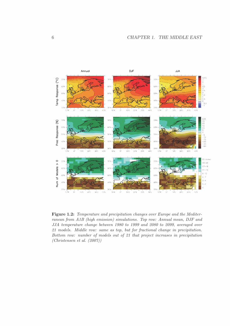
Figure 1.2: Temperature and precipitation changes over Europe and the Mediter-ranean from A1B (high emission) simulations. Top row: Annual mean, DJF andJJA temperature change between 1980 to 1999 and 2080 to 2099, averaged over21 models. Middle row: same as top, but for fractional change in precipitation.Bottom row: number of models out of 21 that project increases in precipitation(Christensen et al. (2007))

1.3. CLIMATE CHANGE PREDICTIONS 7

an increase of between 1.5 to 3.7◦C in summer and 2.0 to 3.1◦C in winter

(predictions based on climate models used in the recent Intergovernmental

Panel on Climate Change (IPCC) report, ranging between lowest and highest

greenhouse gas emissions scenarios, Cruz et al. (2007)). Higher temperatures

will change patterns and amounts of precipitation - shown in figure (1.2) are

projected changes in temperature and precipitation in the 21st century over

Europe under an A1B (high emission) scenario (Christensen et al. (2007)).

Models predict that the region including the Mediterranean, stretching from

the strait of Gibraltar eastwards to Turkey and the Middle East will get

drier. In the Middle East significant rainfall declines in winter will outweigh

slight increases during the dry summer (Cruz et al. (2007)). One study

has predicted that future precipitation reduction will be sufficient that the

Fertile Crescent will lose its current shape and may even disappear (Kitoh

et al. (2008)). The NAO is also predicted to become more positive in a future

climate, which would further decrease winter rainfall Cullen et al. (2002).

The region is also set to experiencE an increase in extreme rainfall events

(Alpert et al. (2008)). It is predicted that the dominant precipitation mech-

anism will shift from direct dependence on storm tracks and toward greater

precipitation triggering by upslope flow of moist air masses (Evans (2009)).

This is in agreement with the predicted reduction in the strength of the

Mediterranean storm track in a future climate (Bengtsson & Hodges (2006)).

Furthermore there may be small northward movement of the intertropical

convergence zone (ITCZ) which would change the atmospheric stability over

the Saudi desert and could trigger increases in precipitation in some areas

(Evans (2009)).

When combined with population pressures and already strained water

resources, these future predictions of precipitation reduction in vital hydro-

logical areas do not paint a good picture for the people of the region in the

next century. However, forewarned is forearmed and increases in reliabil-

ity and accuracy of climate change predictions will help management of a


dwindling resource. This study focuses on precipitation in climate models

and specifically how the current trend toward higher spatial resolution will

improve the accuracy of precipitation predictions. The questions upon which

this study focus are laid out in the next section.

1.4 Aims of the study

There are many conceptual models of the climate, ranging from simple radia-

tion budget models which can predict an average global equilibrium temper-

ature, up to spatially and temporally discretised global circulation models.

Predictions of climate change come primarily from coupled ocean-atmosphere

global climate models (Thorpe (2005)). These are mathematical models, the

most basic of which solve the fluid equations of motion for the atmosphere on

a 3 dimensional grid over time (climate models are described in more detail

in chapter 2). The size of grid upon which the equations are solved varies

between models and is of vital importance. Too low a resolution and weather

systems cannot be adequately resolved; too high and the computing cost can

become prohibitive.

In this report the output from two high resolution models for the Middle

East is studied. One is HiGEM, a global coupled model developed by the

Natural Environment Research Council (NERC), the UK academic commu-

nity and the Met Office Hadley Centre. The other is an atmosphere only

regional climate model (RCM), based on the PRECIS regional climate mod-

eling system, developed at the Hadley Centre. The aims of this study are as

follows:

• To evaluate the performance of the two climate models in representing

rainfall over the Middle East

• To use statistical measures to quantitatively evaluate model skill

1.4. AIMS OF THE STUDY 9

• To investigate how the variation of model skill with resolution might

be represented

In the next chapter the theory and basic ideas behind climate modeling

are discussed, along with a more complete description of the two models used

in this study as well as the observations used for comparison.

Chapter 2

Model description and

observations

Climate models have varying levels of complexity, ranging from simple ra-

diation budget models, through to basic atmosphere only models to Earth

system models which include components for the ocean, the cryosphere, the

biosphere and more. They are widely used to understand and predict the

evolution of the climate and have recently been the key to attributing recent

change in climate to human activities (Slingo et al. (2009)). Before climate

models are used for prediction however, they must be validated against past

observations to verify that they are representing the climate system accu-

rately.

The focus of this chapter is climate modelling and the different types of

models used. The importance of model resolution for the representation of

climate is discussed. Finally the two models used in this study are described,

as well as the different observational datasets used for validation against the

models.

10

2.1. CLIMATE MODELLING 11

2.1 Climate Modelling

A climate model is an attempt to represent the many processes that produce

climate in a mathematical model. The aim is to understand these processes

and predict the effects of changes in interactions. This is accomplished by

describing the system in terms of basic physical principles, reduced to math-

ematical laws, which can be numerically solved on a spatial grid (McGuffie

& Henderson-Seller (2005)). General circulation models (GCMs) are one

kind of model, which incorporate the three–dimensional nature of the atmo-

sphere by discretising in space and time. They can be either atmosphere

only (AGCM) or ocean only (OGCM) whereby interactions with the miss-

ing component of the system are forced externally. However many state of

the art climate models are fully coupled, they have atmospheric and oceanic

components and interactions between them are generated internally by the

model.

The fundamental laws solved in GCMs are conservation laws: conserva-

tion of energy, conservation of momentum and conservation of mass. The

ideal gas law is also solved, and dynamics are described by the primitive

equations (an approximated form of the navier–stokes equations) on a rotat-

ing sphere. Generally equations are solved to give the mass movement (i.e.

wind field or ocean currents) at the next timestep, but models also include

processes such as cloud and sea ice formation and heat, moisture and salt

transport (McGuffie & Henderson-Seller (2005)). Some components of the

climate system such as convective clouds, cloud microphysics and subgrid

scale eddies occur on too small a scale to be resolved explicitly by climate

models and so are represented in models by simplified mathematical formulae

(Peixoto (2007)). This is known as parametrization.

Similar to GCMs are regional climate models (RCMs), which generally use

the same equations as GCMs but are applied over a limited area, rather than

the whole globe. Because they do not model the whole globe they are less

12 CHAPTER 2. MODEL DESCRIPTION AND OBSERVATIONS

computationally expensive and so are able to operate at higher resolutions

and generate high resolution output for studying global change (Wang et al.

(2004)). At their boundaries they are generally ‘driven’ by a GCM or by

observed data, whereby fields at the lateral boundaries are given the same

values as the driving GCM/observational data.

2.1.1 Model Resolution

Climate modelling grew out of numerical weather prediction (NWP) more

than 40 years ago. Since then climate models have become increasingly com-

plex with extra components of the climate system being added. Because of

this, unlike NWP models which have steadily increased in spatial resolution,

until recently climate models have still operated on regular grids of the order

200–300km (Slingo et al. (2009)). At this scale models cannot adequately

resolve weather systems such as mid–latitude fronts and tropical cyclones.

However improvements in computing capability mean that higher resolution

models have recently developed and are becoming more common (Slingo et al.

(2009)).

Increasing the resolution of climate models means that weather systems

are better represented (Catto et al. (2009)). Higher resolution in the atmo-

sphere and ocean has been shown to allow coupling to occur on small spatial

scales, and small scale interactions can be more realistically captured (Shaf-

frey et al. (2009)). This, along with other high resolution benefits such as

more detailed orography will hopefully result in more accurate representa-

tion of precipitation processes in climate models. The hope is that climate

will be more accurately represented through better representation of weather

systems, regional circulation, topography and heterogeneity in land cover.

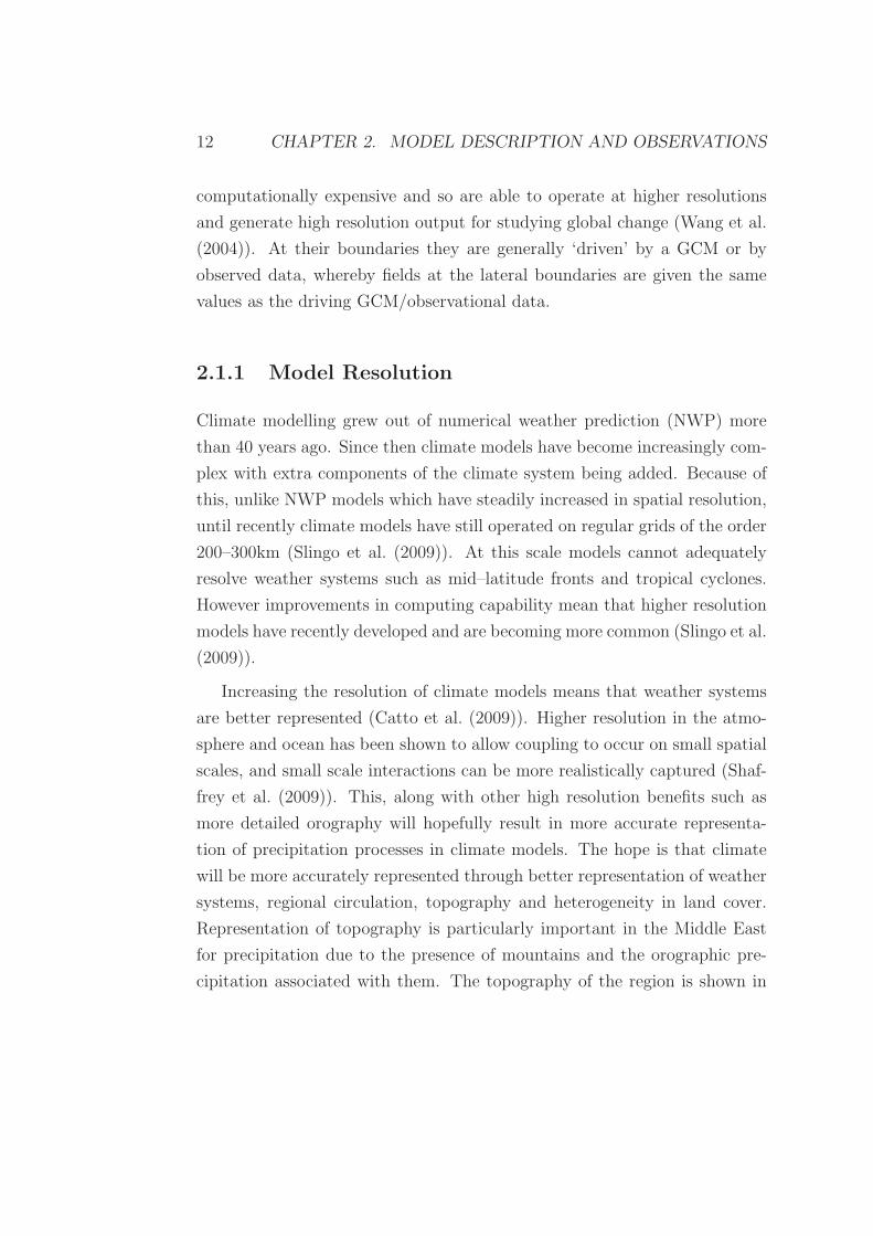
Representation of topography is particularly important in the Middle East

for precipitation due to the presence of mountains and the orographic pre-

cipitation associated with them. The topography of the region is shown in

2.2. DESCRIPTION OF MODELS 13

figure 2.1, along with the topography as it is represented by the two models

used in this study.

Whilst the move towards higher resolution goes on (some atmosphere-

only models now operate at resolutions of 20km (Kitoh et al. (2008))), it

may be that the cost of the extra computing power will outweigh the increase

of skill gained by moving to higher resolutions. In NWP this is especially a

problem since a move to smaller scales results in forecast errors growing more

rapidly, and so higher resolution many not give any significant increase in

model skill (Lorenz (1969), Done et al. (n.d.), Mass et al. (2002)). Because of

these issues, a new scale-selective method for evaluating NWP precipitation

forecasts has recently been introduced (Roberts & Lean (2008)). This novel

method has been modified in this study and implemented to the output of

climate models rather than NWP models. The theory is discussed in section

4.2.

2.2 Description of models

Two models are used in this study; HiGEM, an atmosphere–ocean coupled

GCM, and an atmosphere–only RCM. The main differences in the models

are detailed in table 2.1. Further details of the models are described below.

2.2.1 HiGEM

HiGEM is a global coupled model, developed by NERC, the UK academic

community and the Met Office Hadley Centre. It based on the latest config-

uration of the UK Met Office Unified Model, HadGEM1 which contributed

to the IPCC 4th Assessment Report (Solomon et al. (2007)).

The horizontal resolution of HadGEM1 is 1.875◦ x 1.25◦ in longitude and

latitude in the atmosphere, and 1◦ x 1◦ (increasing to 1/3◦ meridionally near


Figure 2.1: Topography of the region (top), as represented by the regional model(middle) and by HiGEM (bottom). Units are m.

2.2. DESCRIPTION OF MODELS 15

HiGEM Regional ModelRegion Whole globe Europe, Mediterranean &

Middle East

Components Coupled atmosphere andocean

Atmosphere only

Resolution 1.25◦ x 0.83◦ for atmo-sphere 1/3◦ x 1/3◦ for theocean

0.44◦ x 0.44◦

Vertical levels 38 in atmosphere, 40 inthe ocean

19

Lateral bound-ary conditions

None needed From HadAM3P

Table 2.1: Comparison of the two models used in this study.

the equator) in the ocean. In HiGEM this has been increased to 1.25◦ x 0.83◦

in longitude and latitude for the atmosphere, and 1/3◦ x 1/3◦ globally for

the ocean and sea ice. The timestep of the model is 20 minutes (Shaffrey

et al. (2009)).

The atmosphere of HiGEM has 38 levels in the vertical. The top of the

model is at 39km, which means the stratosphere is not well resolved. The

ocean component has 40 unevenly spaced levels in the vertical with enhanced

resolution near the surface to better resolve the mixed layer and atmosphere-

ocean interaction processes. The maximum ocean depth is 5500m (Shaffrey

et al. (2009)).

The orography is derived from the 1’ GLOBE dataset, which provides an

accurate representation of the mountains and their sub-gridscale character-

istics (Shaffrey et al. (2009)). The topography as it is represented in HiGEM


is shown in figure 2.1.

Climatologies are based on years 21–70 of a model run, so that the upper

ocean and atmosphere have sufficient time to spin up. Initial conditions have

been given to the model to simulate climate over the past half century.

2.2.2 The Regional Climate Model

The RCM used in this study is based on PRECIS, a model based on HadAM3P,

a global, atmosphere-only model developed at the Hadley Centre. The RCM

has a horizontal resolution of 0.44◦, giving a grid spacing of 50km. This

permits a large domain to be used whilst representing significantly more to-

pographic variation than is possible in the 200km scale of the generation of

climate models used in IPCC (Black (2009), Slingo et al. (2009)) (topography

as represented by the RCM is shown in figure 2.1). The model has 19 levels

in the vertical and includes the whole Mediterranean so that cyclones which

bring most of the rain to the Middle East do not travel through the domain

boundary (Black (2009)). The domain of the model is shown in figure 2.2.

It should be noted that there are normally problems associated with model

output close to the boundary, therefore when the RCM will be evaluated

only output at some distance from the boundary will be looked at.

RCMs are applied over a limited area and so require input at both the

surface and lateral boundaries of the domain. Lateral boundary conditions

were derived from integrations of HadAM3P forced with surface boundary

conditions (sea surface temperature, sea ice fraction), which were derived

from observations. Boundary conditions for the PRECIS RCM are on a grid

of 2.5◦ latitude x 3.75◦ longitude, about 300 km resolution at 45N or 400

km at the equator. Surface boundary conditions for the RCM are based on

HadCM3 predictions and observations (Black (2009)).

2.3. DESCRIPTION OF OBSERVATIONS 17

Figure 2.2: The domain over which the regional model is evaluated.

2.3 Description of observations

Compared with many places in the world, the Middle East is a data sparse

area (Evans (2004)). As such, several different observational datasets, each

with their own advantages and disadvantages, have been used.

The global precipitation dataset from the global precipitation climatology

centre (GPCC) is used. This data is based upon quality controlled ground

station data from up to 43,000 stations, with irregular coverage in time.

These provide a 1◦ x 1◦ resolution precipitation climatology for the period

1951 to 2004 (Earth System Research Laboratory (2009)).

Global precipitation climatology project (GPCP) data are also used. This

consists of data from over 6,000 rain gauge stations, satellite geostationary

and low-orbit infrared, passive microwave, and sounding observations which

are merged to estimate monthly rainfall on a 2.5◦ global grid from 1979 to

the present (NASA Goddard Space Flight Center (2009)).

Finally, observations from the tropical rainfall measuring mission (TRMM)

satellite are used. This satellite gives a fine spatial resolution of precipitation

(0.25◦ x 0.25◦) around the globe from 50◦ N to 50◦ S. Climatologies are calcu-


lated from 1997 to 2007 and consist of TRMM observations constrained with

gauge station and GPCP data (Huffman, G.J. and Adler, R.L. and Bolvin,

D.T. and Gu, G. and Nelkin, E.J. and Bowman, K.P. and Hong, Y. and

Stocker, E.F. and Wolff, D.B. (2007)).

To compare mean sea level pressure and wind fields in the models, data

from ERA-40 reanalysis was used. ERA reanalysis is a dataset created by

assimilating many sources of observations into the ECMWF climate model

at a 40km resolution (Uppala et al. (2005)).

Chapter 3

Visual comparison of

climatologies

HiGEM and the Regional Climate Model have been run to produce clima-

tologies over the Middle East. These climatologies give average values of

meteorological variables for the domains over which they are run. Although

the focus of this study is specifically to investigate how well the models repre-

sent precipitation, it is important to evaluate how well the models represent

other aspects of the climate system. This is because there are different cli-

matological processes that cause precipitation and so how a model represents

precipitation is dependent on how well it represents these processes, which

are dependent on other meteorological variables.

In this chapter model climatologies for precipitation, 10m surface wind

fields and mean sea level pressure are plotted and visually compared to clima-

tologies taken from a variety of observations. Several observational datasets

for precipitation have been plotted which have their own advantages and

disadvantages; these are discussed.

19

20 CHAPTER 3. VISUAL COMPARISON OF CLIMATOLOGIES

3.1 Precipitation

3.1.1 Comparing observations

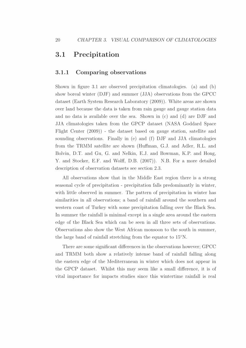
Shown in figure 3.1 are observed precipitation climatologies. (a) and (b)

show boreal winter (DJF) and summer (JJA) observations from the GPCC

dataset (Earth System Research Laboratory (2009)). White areas are shown

over land because the data is taken from rain gauge and gauge station data

and no data is available over the sea. Shown in (c) and (d) are DJF and

JJA climatologies taken from the GPCP dataset (NASA Goddard Space

Flight Center (2009)) - the dataset based on gauge station, satellite and

sounding observations. Finally in (e) and (f) DJF and JJA climatologies

from the TRMM satellite are shown (Huffman, G.J. and Adler, R.L. and

Bolvin, D.T. and Gu, G. and Nelkin, E.J. and Bowman, K.P. and Hong,

Y. and Stocker, E.F. and Wolff, D.B. (2007)). N.B. For a more detailed

description of observation datasets see section 2.3.

All observations show that in the Middle East region there is a strong

seasonal cycle of precipitation - precipitation falls predominantly in winter,

with little observed in summer. The pattern of precipitation in winter has

similarities in all observations; a band of rainfall around the southern and

western coast of Turkey with some precipitation falling over the Black Sea.

In summer the rainfall is minimal except in a single area around the eastern

edge of the Black Sea which can be seen in all three sets of observations.

Observations also show the West African monsoon to the south in summer,

the large band of rainfall stretching from the equator to 15◦N.

There are some significant differences in the observations however; GPCC

and TRMM both show a relatively intense band of rainfall falling along

the eastern edge of the Mediterranean in winter which does not appear in

the GPCP dataset. Whilst this may seem like a small difference, it is of

vital importance for impacts studies since this wintertime rainfall is real

3.1. PRECIPITATION 21

and can be seen from rainfall gauge data (Sharon & Kutiel (1986), Black

(2009)). In particular it falls along the length of the Jordan river, upon which

many communities depend heavily. Moving eastward from the Mediterranean

across Israel and towards the desert there is a sharp gradient in rainfall

contour lines, which is almost totally absent in the GPCP data. It is for

this reason, along with the fact that GPCP has the lowest resolution of all

observations, that the GPCP data will not be used for statistical comparison

with the models – attempting to verify a model against observations is a

misleading exercise if the observations do not match reality in important

areas. The GPCC and TRMM datasets show generally the same pattern

of precipitation – they both show the rainfall falling near the Jordan river,

they both capture the orographic precipitation in Taurus mountains of South

Eastern Turkey where the Euphrates and Tigris begin their journey toward

the Persian Gulf and they both capture the wintertime rainfall over the

Fertile Crescent.

The GPCC dataset however does not have data over the seas since it

comes only from ground stations. It also has a lower resolution than TRMM,

which shows a more detailed pattern of precipitation. Conversely, the TRMM

climatology is calculated over the shortest time period (1997–2007) whereas

the GPCC and GPCP data stretch back over longer time periods (starting

from 1951 and 1979 respectively). It is thought however that when it comes

to statistical analysis, the advantages of TRMM over the other datasets out-

weigh the disadvantage of having been calculated over a shorter time period.

The TRMM data will therefore be used for model validation.

3.1.2 Looking at the models

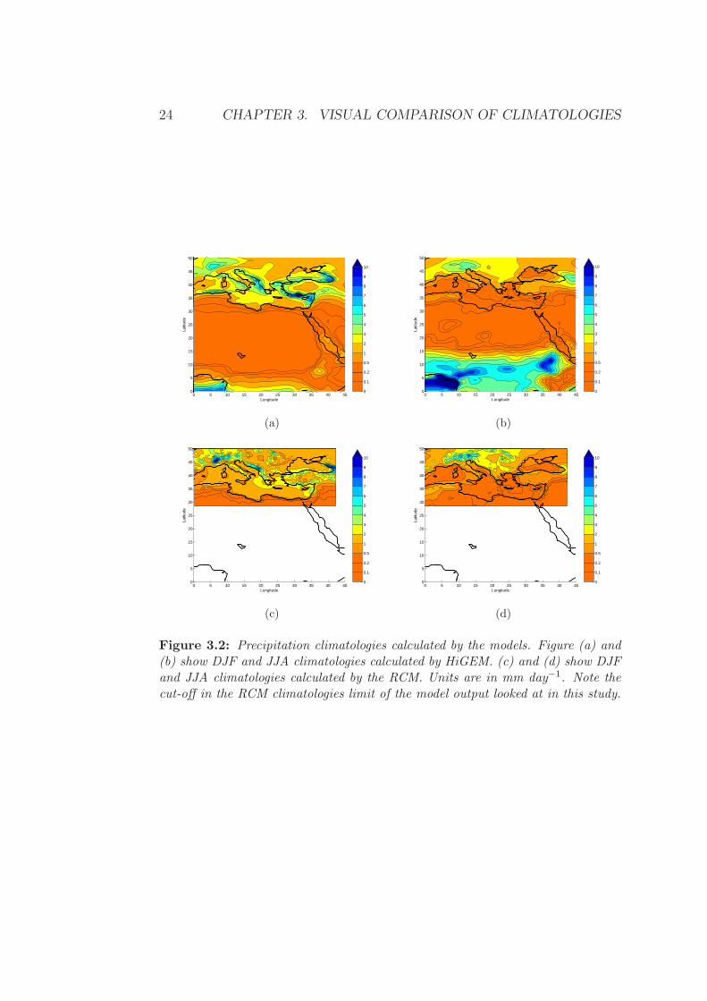
Shown in figure 3.2 are precipitation climatologies for the models. (a) and

(b) show DJF and summer JJA climatolgoies calculated by HiGEM. (c) and

(d) show DJF and JJA climatologies calculated by the RCM. HiGEM fields


0

0.1

0.2

0.5

1

2

3

4

5

6

7

8

9

10

0 5 10 15 20 25 30 35 40 450

5

10

15

20

25

30

35

40

45

50

Longitude

Latit

ude

(a)

0

0.1

0.2

0.5

1

2

3

4

5

6

7

8

9

10

0 5 10 15 20 25 30 35 40 450

5

10

15

20

25

30

35

40

45

50

Longitude

Latit

ude

(b)

0

0.1

0.2

0.5

1

2

3

4

5

6

7

8

9

10

0 5 10 15 20 25 30 35 40 450

5

10

15

20

25

30

35

40

45

50

Longitude

Latit

ude

(c)

0

0.1

0.2

0.5

1

2

3

4

5

6

7

8

9

10

0 5 10 15 20 25 30 35 40 450

5

10

15

20

25

30

35

40

45

50

Longitude

Latit

ude

(d)

0

0.1

0.2

0.5

1

2

3

4

5

6

7

8

9

10

0 5 10 15 20 25 30 35 40 450

5

10

15

20

25

30

35

40

45

50

Longitude

Latit

ude

(e)

0

0.1

0.2

0.5

1

2

3

4

5

6

7

8

9

10

0 5 10 15 20 25 30 35 40 450

5

10

15

20

25

30

35

40

45

50

Longitude

Latit

ude

(f)

Figure 3.1: Precipitation climatologies from observations. Figure (a) and(b) show boreal winter (DJF) and summer (JJA) climatologies from the GPCCdataset. (c) and (d) show DJF and JJA climatologies from GPCP data and (e)and (f) show climatologies from TRMM. Units are in mm day−1. The lack of ob-servations over the ocean in the GPCC climatologies is due to observations havingbeen taken from ground stations only.

3.2. MEAN SEA LEVEL PRESSURE 23

are smoother than the RCM due to the lower resolution of the model and

the extent of the RCM fields show the spatial limits of the modelled area.

Both models capture the seasonal cycle in precipitation with all rainfall

falling in winter and little in summer. They also both capture the general

shape of the winter precipitation around the coastlines of Turkey and to some

extent the small area of summer rainfall over the Eastern coast of the Black

Sea – in the RCM this is present, but lower than that seen in either HiGEM

or observations.

HiGEM however overestimates precipitation around the south/south east-

ern coast of Turkey and slightly overestimates it over the Fertile Crescent.

The RCM has significantly less precipitation in the region compared to ob-

servations, especially at the coasts.

Both models capture some amount of detail of the gradient of the pre-

cipitation contours around the eastern Mediterranean – HiGEM shows the

gradient as slightly sharper than observations (TRMM & GPCC), whereas

the gradient in the RCM is slightly smaller due to the underprediction of

precipitation on the coast.

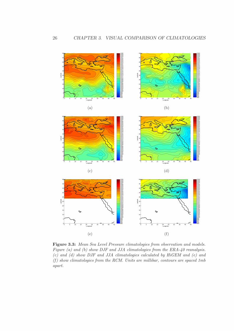
3.2 Mean Sea Level Pressure

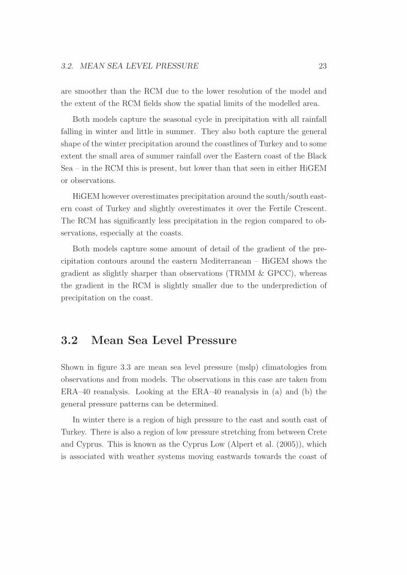
Shown in figure 3.3 are mean sea level pressure (mslp) climatologies from

observations and from models. The observations in this case are taken from

ERA–40 reanalysis. Looking at the ERA–40 reanalysis in (a) and (b) the

general pressure patterns can be determined.

In winter there is a region of high pressure to the east and south east of

Turkey. There is also a region of low pressure stretching from between Crete

and Cyprus. This is known as the Cyprus Low (Alpert et al. (2005)), which

is associated with weather systems moving eastwards towards the coast of


0

0.1

0.2

0.5

1

2

3

4

5

6

7

8

9

10

0 5 10 15 20 25 30 35 40 450

5

10

15

20

25

30

35

40

45

50

Longitude

Latit

ude

(a)

0

0.1

0.2

0.5

1

2

3

4

5

6

7

8

9

10

0 5 10 15 20 25 30 35 40 450

5

10

15

20

25

30

35

40

45

50

Longitude

Latit

ude

(b)

0

0.1

0.2

0.5

1

2

3

4

5

6

7

8

9

10

0 5 10 15 20 25 30 35 40 450

5

10

15

20

25

30

35

40

45

50

Longitude

Latit

ude

(c)

0

0.1

0.2

0.5

1

2

3

4

5

6

7

8

9

10

0 5 10 15 20 25 30 35 40 450

5

10

15

20

25

30

35

40

45

50

Longitude

Latit

ude

(d)

Figure 3.2: Precipitation climatologies calculated by the models. Figure (a) and(b) show DJF and JJA climatologies calculated by HiGEM. (c) and (d) show DJFand JJA climatologies calculated by the RCM. Units are in mm day−1. Note thecut-off in the RCM climatologies limit of the model output looked at in this study.

3.2. MEAN SEA LEVEL PRESSURE 25

the Mediterranean, bringing wintertime rainfall.

In summer the pressure drops, and the pattern observed is a region of

low pressure eastwards towards the Persian Gulf, which increases rapidly

northwards and westwards creating a high gradient of pressure associated

with high wind speeds through geostrophic balance. A long tongue of low

pressure can also be seen in summer, extending westwards from Northern

Iraq towards Cyprus and over the Mediterranean. HiGEM pressure fields are

shown in 3.3(c) and 3.3(d). It captures the pressure patterns fairly well; the

general pattern of high–low pressure between the North East of the domain

and Cyprus can be seen. It also captures some of the spatial shape of the

summertime low pressure tongue.

The Cyprus Low is represented in HiGEM, although its spatial extent and

intensity is underestimated in the model. The maximum of the low appears

over the South West coast of Turkey, with a pressure of one or two millibars

greater than that from ERA. The pattern of summer pressure is captured

well, the shape of the sharp gradients is represented accurately, however the

intensity of the low pressure east of the Mediterranean is less intense than

ERA.

RCM pressure fields are shown in 3.3(e) and 3.3(f). The RCM captures

summer pressure patterns well, both in shape and intensity. Winter patterns

however do not show the intensity of the high pressure over Turkey and it can

be seen that the Cyprus Low is not well represented in the model climatology.


9959969979989991000100110021003100410051006100710081009101010111012101310141015101610171018101910201021102210231024102510261027102810291030

0 5 10 15 20 25 30 35 40 450

5

10

15

20

25

30

35

40

45

50

Longitude

Latit

ude

(a)

9959969979989991000100110021003100410051006100710081009101010111012101310141015101610171018101910201021102210231024102510261027102810291030

0 5 10 15 20 25 30 35 40 450

5

10

15

20

25

30

35

40

45

50

Longitude

Latit

ude

(b)

9959969979989991000100110021003100410051006100710081009101010111012101310141015101610171018101910201021102210231024102510261027102810291030

0 5 10 15 20 25 30 35 40 450

5

10

15

20

25

30

35

40

45

50

Longitude

Latit

ude

(c)

9959969979989991000100110021003100410051006100710081009101010111012101310141015101610171018101910201021102210231024102510261027102810291030

0 5 10 15 20 25 30 35 40 450

5

10

15

20

25

30

35

40

45

50

Longitude

Latit

ude

(d)

9959969979989991000100110021003100410051006100710081009101010111012101310141015101610171018101910201021102210231024102510261027102810291030

0 5 10 15 20 25 30 35 40 450

5

10

15

20

25

30

35

40

45

50

Longitude

Latit

ude

(e)

9959969979989991000100110021003100410051006100710081009101010111012101310141015101610171018101910201021102210231024102510261027102810291030

0 5 10 15 20 25 30 35 40 450

5

10

15

20

25

30

35

40

45

50

Longitude

Latit

ude

(f)

Figure 3.3: Mean Sea Level Pressure climatologies from observation and models.Figure (a) and (b) show DJF and JJA climatologies from the ERA-40 reanalysis.(c) and (d) show DJF and JJA climatologies calculated by HiGEM and (e) and(f) show climatologies from the RCM. Units are millibar, contours are spaced 1mbapart.

3.3. SURFACE WIND PATTERNS 27

3.3 Surface Wind Patterns

3.3.1 Observed Wind Fields

Shown in figure 3.4 are climatological 10m surface wind patterns from ob-

servations and from models. The observations for DJF and JJA are from

ERA-40 reanalysis and are shown in (a) and (b).

The observed winter wind field show relatively low speeds over the much

of the land of the Middle East. Strong westerly winds can be seen over the

Mediterranean. This is the Mediterranean storm track. Where this meets

the land there is slight north easterly flow, which, upon meeting the moist

air from the Mediterranean generates convergence and ascent. Since this

air holds moisture from passing over the sea, precipitation results, which

is observed in this general area. Relatively strong northerly winds are also

observed over the Aegean. Winds are generally stronger since the sea surface

is generally smoother than the rougher land surface, so winds passing over

the sea experience less friction.

The wind patterns are also consistent with the pressure patterns, with

wind moving counter-clockwise around the Cyprus low in winter. This can

be seen in the westerly Mediterranean storm track and also in the south

westerly movement of air over the land to the east of the Mediterranean.

There is no corresponding easterly flow to the north however, this could

possibly be due to the presence of the Taurus mountains which would hinder

any horizontal movement of air.

In summer the wind also follows the pressure patterns, moving counter-

clockwise around the strong low pressure area, with greater speeds due to the

stronger presssure gradient. Winds over the Mediterranean also have more of

a northerly component than in winter. Furthermore, over Turkey the winds

are northerly, whereas in winter there is no net wind.


There is also very strong northerly flow over north east Africa in summer;

this movement of air away from the Mediterranean could be a factor behind

the lack of precipitation; air carrying moisture is moving away from the region

before it has a chance to cause precipitation. The air then flowing over the

Middle East would then be fairly dry since it would not have travelled far

over water.

3.3.2 Modelled Wind Fields

10m surface wind fields calculated by HiGEM for DJF & JJA are in (c) and

(d) of figure 3.4 and results for the RCM are in (e) and (f). Fields calculating

by subtracting ERA wind fields from model output are shown in figure 3.5.

The direction and magnitude of the arrows in these plots show the direction

and magnitude of the errors in the modelled fields.

HiGEM captures the general patterns in winter, however it underesti-

mates the magnitude of winds in the Mediterranean storm track. It also fails

to capture the northerly flow over the Aegean. It captures well however the

north easterly convergence–causing flow in the south east of Turkey, which is

in fact overestimated in the model which can be seen from the convergence

in the errors seen in figure 3.5(a). This extra convergence would cause extra

ascent in the model, which could well be a factor in the overestimation of

precipitation seen in HiGEM in the area. The general summer flow is cap-

tured fairly well in HiGEM, however the strength of the Mediterranean storm

track is underestimated. This could be associated with the underestimation

in intensity of the low pressure patterns east of the Mediterranean described

in section 3.2; less intense low pressure would cause a weaker circulation.

The RCM underestimates the strength of the Mediterranean storm track

in winter. Furthermore, it overestimates the westerly flow east of the Mediter-

ranean and shows a slight northerly flow over Turkey. These errors can be

seen to diverge outwards from the region of precipitation, seen clearly in fig-

3.3. SURFACE WIND PATTERNS 29

0

1

2

3

4

5

6

20 25 30 35 40 4525

30

35

40

45

50

Longitude

Latit

ude

(a)

0

1

2

3

4

5

6

20 25 30 35 40 4525

30

35

40

45

50

Longitude

Latit

ude

(b)

0

1

2

3

4

5

6

20 25 30 35 40 4525

30

35

40

45

50

Longitude

Latit

ude

(c)

0

1

2

3

4

5

6

20 25 30 35 40 4525

30

35

40

45

50

Longitude

Latit

ude

(d)

0

1

2

3

4

5

6

20 25 30 35 40 4525

30

35

40

45

50

Longitude

Latit

ude

(e)

0

1

2

3

4

5

6

20 25 30 35 40 4525

30

35

40

45

50

Longitude

Latit

ude

(f)

Figure 3.4: Climatological 10m surface wind fields from observation and models.Figure (a) and (b) show DJF and JJA wind patterns from ERA-40 reanalysis. (c)and (d) show DJF and JJA wind patterns calculated by HiGEM and (e) and (f)show results from the RCM. Units are ms−1, arrow sizes are proportional to windspeed.


0

0.5

1

1.5

2

2.5

3

20 25 30 35 40 4525

30

35

40

45

50

Longitude

Latit

ude

(a)

0

0.5

1

1.5

2

2.5

3

20 25 30 35 40 4525

30

35

40

45

50

Longitude

Latit

ude

(b)

0

0.5

1

1.5

2

2.5

3

20 25 30 35 40 4525

30

35

40

45

50

Longitude

Latit

ude

(c)

0

0.5

1

1.5

2

2.5

3

20 25 30 35 40 4525

30

35

40

45

50

Longitude

Latit

ude

(d)

Figure 3.5: Errors in 10m surface wind fields between models and ERA-40 reanal-ysis. Figure (a) and (b) show DJF and JJA wind field errors found by subtractingERA fields from HiGEM. (c) and (d) show DJF and JJA wind field errors foundby subtracting ERA fields from the RCM fields. Units are ms−1, arrow sizes areproportional to wind speed.

3.4. DISCUSSION 31

ure 3.5(c). This would cause a smaller convergence at ground level than is

seen in observations, causing less ascent and therefore less precipitation. This

is then potentially a factor in the lack of precipitation observed in the area,

described in section 3.1.2. Errors are larger in summer, with the RCM pre-

dicting over–northerly flow over most of the domain. The overestimation of

the magnitude of the westerly flow over the desert east of the Mediterranean

is one of the two largest sources of error in the model, along with a north–

easterly flow in the north–east of the domain, where the ERA reanalysis has

almost no wind.

3.4 Discussion

Both models represent the seasonal cycle of precipitation well, and are suc-

cessful in capturing the general spatial pattern. However HiGEM overes-

timates the total amount of precipitation and the RCM underestimates it.

Both models also underestimate the magnitude of the winds making up the

Mediterranean storm track which is associated with the Cyprus low, which

is underestimated in HiGEM and even moreso in the RCM.

Both models have errors in wind fields around the main region of precipi-

tation around the east coast of the Mediterranean, with HiGEM overestimat-

ing convergence in the region and the RCM underestimating it. This could

well be associated with the errors in precipitation amounts; extra conver-

gence in HiGEM would give extra ascent and so give too much precipitation,

and a lack of convergence in the RCM would give less ascent and so less

precipitation.

Visual comparison of climatologies has allowed a qualitative evaluation

of model performance. However it is useful exercise to evaluate quantitative,

statistical, measures of model skill to pin down specific areas of weakness or

strength in the model. This is addressed in the following chapter.

Chapter 4

Statistical verification methods

The output from the two models has been compared visually with observa-

tions and qualitative distinctions have been drawn. Quantitative measures

of differences between models and reality can be obtained by using statistical

measures of skill. In this chapter several standard measures are described

- the bias, the root mean square error and the pattern correlation. A new

method for evaluating how model skill varies with spatial scale is also de-

scribed. This has been adapted for climate modelling from a new method

recently implemented by Roberts and Lean for numerical weather prediction

(Roberts & Lean (2008)).

4.1 Statistical measures of model skill

Bias has been used to evaluate model performance against observations, it is

calculated as

Bias = M − O (4.1)

where M is the spatial mean of a modelled value over a domain and O is

the spatial mean of observed values. This measures the amount by which

32

4.2. FRACTIONS SKILL SCORES 33

the model over or underestimates the average value of a parameter over a

domain.

Root mean square error (RMSE) is given by

RMSE =

√

√

√

√

1

N

N∑

i=1

(Oi − Mi)2 (4.2)

where N is the number of observed (O) and modelled (M) values being

compared. Here N is the number of grid boxes in the domain. The RMSE is

a basic measure of accuracy, with a lower value indicating a more accurate

field

The pattern correlation is also used, which is the correlation of a series

of data points from the observed field with corresponding values from the

modelled field at a fixed time,

ρ =

∑N

i=1 (Oi − O)(Mi − M)√

∑N

i=1 (Oi − O)2

√

∑N

i=1 (Mi − M)2

, (4.3)

where sums are carried out over all grid boxes. A value of ρ = 1 represents a

modelled field identical to observations, decreasing to ρ = 0 for no correlation.

4.2 Fractions Skill Scores

Higher model resolution does not necessarily mean better objectively scored

accuracy (Roberts & Lean (2008)). In NWP this is especially a problem

since a move to smaller scales results in forecast errors growing more rapidly,

and so higher resolution many not give any significant increase in model skill

(Lorenz (1969), Done et al. (n.d.), Mass et al. (2002)). Because of these

issues, a new scale-selective method for evaluating NWP precipitation fore-

casts has recently been introduced (Roberts & Lean (2008)). Using fractions

34 CHAPTER 4. STATISTICAL VERIFICATION METHODS

skill scores this method allows determination of the spatial scales at which

forecasts become skilful. It uses the concept of nearest neighbours as the

means of selecting the scales of interest and is applied to thresholds. The re-

sult is a measure of forecast skill, Fractions Skill Score (FSS), against spatial

scale for each threshold. This verification method described in their work is

reproduced here.

4.2.1 Conversion to binary fields

Observed and modelled rainfall fields are first projected onto the same grid.

In this case since the TRMM observations have a higher resolution, these are

projected onto each of the model grids. A threshold (q) is chosen and used to

convert the fields into binary fields (IO) and (IM). All grid points exceeding

the threshold are assigned a value of 1 and all others a value of 0, i.e.,

IO =

{

1 Or ≥ q

0 Or < q

,

with a parallel result for IM . An illustration of binary fields is shown in

figure 4.1.

4.2.2 Generation of fractions

The binary fields are then converted to fractions. For every grid point in

the binary fields obtained from equation (4.2.1) the fraction of surrounding

points within a given square of length n that have a value of 1 (i.e. that have

exceeded the threshold) is calculated. This is described for the observed field

by


(a) (b)

(c) (d)

Figure 4.1: Example binary conversion applied to winter precipitation outputfrom HiGEM. Shown in (a) the model output and in (b) (c) and (d) are binaryfields calculated for thresholds 1mm day−1, 2mm day−1 and 4mm day−1 respectively(grey areas are 1’s, white areas 0’s).


O(n)(i, j) =1

n2

n∑

k=1

n∑

l=1

I0

[

i + k − 1 −(n − 1)

2, j + l − 1 −

(n − 1)

2

]

, (4.4)

with a similar result for the modelled fractions, M(n)(i, j). Here i goes

from 1 to Nx, where Nx is the number of columns in the domain and j goes

from 1 to Ny, where Ny is the number of rows.

This creates a resultant field of observed fractions, O(n)(i, j), for a square

of length n obtained from the binary field IO and a similar field M(n)(i, j) for

the modelled fractions obtained from the binary field IM .

Fractions are generated for different spatial scales by changing the value

of n, which can be any odd value up to 2N − 1, where N is the number of

points along the longest side of the domain. A square of length 2N −1 is the

smallest that can encompass all points in the domain for squares centred at

any point in the domain.

Using squares to generate the fractions is equivalent to applying the con-

volution kernel for a mean filter to the binary field, which is something often

used in image processing (Roberts & Lean (2008)). Equation (4.4) can be

rewritten as

O(n)(i, j) =n

∑

k=1

n∑

l=1

I0

[

i + k − 1 −(n − 1)

2, j + l − 1 −

(n − 1)

2

]

K(n)(k, l),

(4.5)

where K(n)(k, l) is the n× n kernel for a (square) mean filter. It would also

be possible to use a different kernel such as a circular mean filter or Gaussian

kernel, however only the square filter is used in this study.


4.2.3 Computing fractions skill scores

The mean square error (MSE) for the observed and forecast fractions for a

neighbourhood of length n is given by

MSE(n) =1

NxNy

n∑

i=1

n∑

j=1

[O(n)i,j − M(n)i,j]2. (4.6)

By itself the MSE is highly dependent on the frequency of the event itself. A

MSE skill score has been computed relative to a low-skill reference forecast

(Murphy & Epstein (1989)). This is defined as the fractions skill score (FSS),

FSS(n) =MSE(n) − MSE(n)ref

MSE(n)perfect − MSE(n)ref

= 1 −MSE(n)

MSE(n)ref

, (4.7)

where MSE(n)perf = 0 is the MSE of a perfect forecast for a neighbourhood

length n. The reference used (MSEref ) for each neighbourhood length (n)

is given by

MSE(n)ref =1

NxNy

[

Nx∑

i=1

Ny∑

j=1

O2(n)i,j + M2

(n)i,j

]

. (4.8)

This can be thought of as the largest possible MSE that can be obtained

from the forecast and observed fractions.

Figure 4.2 shows the typical variation of FSS with neighbourhood length

n. It has a range from 0 to 1, a forecast with perfect skill has a score of

1; a score of 0 means zero skill. Skill is lowest at the grid scale, that is,

when the neighbourhood is only one grid point and the fractions are binary

ones or zeros. As the size of the neighbourhood is increased, skill increases

until it reaches an asymptote at n = 2N − 1. If there is no bias, i.e. an

equal number of observed and forecast pixels exceeding the threshold, the

asymptotic fractions skill score (AFSS), which is the FSS at n = 2N − 1,

has a value of 1, indicating perfect skill over the whole domain. If there is a


Figure 4.2: A schematic graph of FSS against spatial scale, from Roberts & Lean(2008).

bias then the observed frequency fO (fraction of observed points exceeding

the threshold over the domain) is not equal to the model-forecast frequency

fM , and from equations (4.6), (4.7) and (4.8) it can be shown that

AFSS = 1 −(fO − fM)2

f 2O + f 2

M

=2fOfM

f 2O + f 2

M

, (4.9)

which can be shown to be less than one for fO 6= fM .

Chapter 5

Statistics of model output

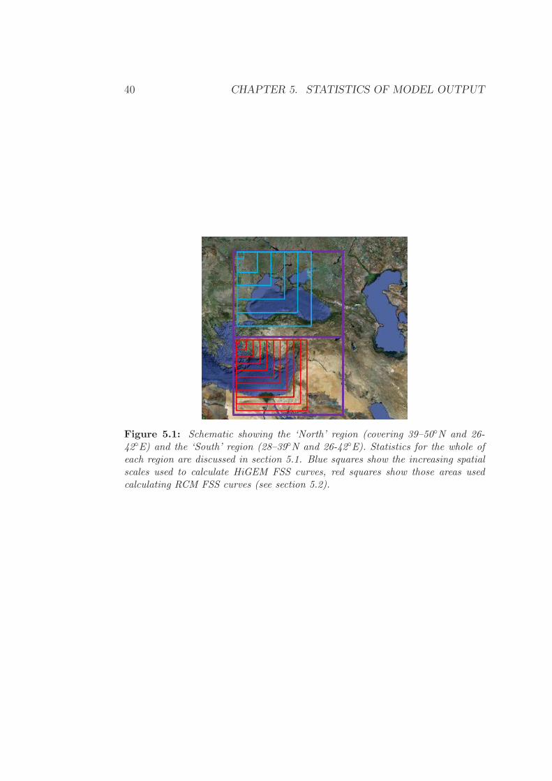
Two regions have been defined; a ‘North’ region, covering 39–50◦N and 26-

42◦E which includes northern Turkey and the Black Sea, and a ‘South’ re-

gion which covers 28–39◦N and 26-42◦E and includes the eastern part of the

Mediterranean and southern Turkey. These regions are shown in figure 5.1.

Statistics described in section 4.1 have been applied to the models described

in section 2.2, using the TRMM dataset as observations. The effect of apply-

ing the convolution kernel on these statistics is also investigated. FSS curves

have been calculated for each region to investigate the effect of horizontal

scale on model skill. These are shown here, and have been calculated for

different rainfall thresholds.

5.1 Standard model skill scores

Statistical results are shown table 5.1. It can be seen that the regional model

has a strong negative bias over both regions, except for summer in the south

region where it has a slight positive bias. This can be seen in figure 3.2(d),

where the regional model predicts some rainfall over the east coast of the

Mediterranean, which is not seen in observations. In the north region HiGEM

39

40 CHAPTER 5. STATISTICS OF MODEL OUTPUT

Figure 5.1: Schematic showing the ‘North’ region (covering 39–50◦N and 26-42◦E) and the ‘South’ region (28–39◦N and 26-42◦E). Statistics for the whole ofeach region are discussed in section 5.1. Blue squares show the increasing spatialscales used to calculate HiGEM FSS curves, red squares show those areas usedcalculating RCM FSS curves (see section 5.2).

5.1. STANDARD MODEL SKILL SCORES 41

Bias (mm day−1) RMSE (mm day−1 P. Corr., ρ

Season - Region HiGEM RCM HiGEM RCM HiGEM RCMDJF - North 0.03 -0.46 1.00 0.90 0.62 0.65JJA - North -0.30 -0.70 0.65 0.90 0.70 0.71DJF - South 0.32 -0.47 1.34 0.86 0.77 0.87JJA - South 0.26 0.13 0.40 0.22 0.87 0.78

Table 5.1: Statistical evaluation of precipitation fields over the two regions.

displays a negative bias in summer, and a very small bias (0.03) in winter.

However it is wrong to think that this indicates perfect performance in the

region, when comparing plots in 3.2(a) and 3.1(e) it can be seen that HiGEM

overestimates precipitation in the south of the region whilst underestimating

it in the north east. These biases cancel each other out, giving a misleadingly

small bias. In the south region HiGEM has positive biases in both seasons.

Root mean square error (RMSE) is somewhat dependent on the magni-

tude of values being compared, since when values are lower, the same relative

error between model and observations would give less of an absolute error

and so contribute less to the RMSE than it would had the values been higher.

This is partly reflected in the lower values in summer than winter over both

models for both regions, apart from the regional model in the north region,

where the values of RMSE are equal. This can be explained by looking at the

2mm day−1 contour in the plots - in observations it encloses a large part of

the domain whereas in the regional model is encloses a much smaller region.

In short; the regional model shows a relatively bad performance in the north

region due to a strong negative bias.

Pattern correlations for both models are similar in both regions, with

both models performing better in the south region. This bodes well for the

use of the models in impacts studies, since the south region contains the

headwaters of the Tigris and Euphrates as well as the Fertile Crescent and

the length of the Jordan - areas where accurate precipitation forecasts are


Bias (mm day−1) RMSE (mm day−1) P. Corr., ρ

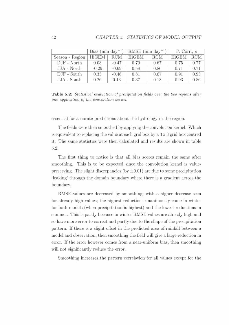
Season - Region HiGEM RCM HiGEM RCM HiGEM RCMDJF - North 0.03 -0.47 0.70 0.67 0.75 0.77JJA - North -0.29 -0.69 0.58 0.86 0.71 0.71DJF - South 0.33 -0.46 0.81 0.67 0.91 0.93JJA - South 0.26 0.13 0.37 0.18 0.93 0.86

Table 5.2: Statistical evaluation of precipitation fields over the two regions afterone application of the convolution kernel.

essential for accurate predictions about the hydrology in the region.

The fields were then smoothed by applying the convolution kernel. Which

is equivalent to replacing the value at each grid box by a 3 x 3 grid box centred

it. The same statistics were then calculated and results are shown in table

5.2.

The first thing to notice is that all bias scores remain the same after

smoothing. This is to be expected since the convolution kernel is value-

preserving. The slight discrepancies (by ±0.01) are due to some precipitation

‘leaking’ through the domain boundary where there is a gradient across the

boundary.

RMSE values are decreased by smoothing, with a higher decrease seen

for already high values; the highest reductions unanimously come in winter

for both models (when precipitation is highest) and the lowest reductions in

summer. This is partly because in winter RMSE values are already high and

so have more error to correct and partly due to the shape of the precipitation

pattern. If there is a slight offset in the predicted area of rainfall between a

model and observation, then smoothing the field will give a large reduction in

error. If the error however comes from a near-uniform bias, then smoothing

will not significantly reduce the error.

Smoothing increases the pattern correlation for all values except for the

5.2. FRACTIONS SKILL SCORES. 43

north region in summer. This can be at least partly attributed to the fairly

uniform nature of the fields; smoothing them would not significantly change

the pattern they show.

5.2 Fractions Skill Scores.

The fields were bias corrected to remove some of the effect of bias on mean

square error, and fractions skill scores, described in section 4.2, were calcu-

lated for both seasons for both models. Scores were calculated for increasing

spatial scales (shown in figure 5.1) for each model. These were calculated for

both the north and south regions. Curves of FSS against spatial scale are

shown in figures 5.2 and 5.3. Different thresholds were used in calculating

the binary fields, q ≥ 0.5, 1, 2 and 4mm day−1, these correspond to (a) &

(b), (c) & (d), (e) & (f) and (g) & (h) respectively for both figures 5.2 and

5.3.

It can be seen that using a lower threshold gives higher FSS scores for all

spatial scales. Furthermore, using a threshold that is greater than the maxi-

mum in the field gives undefined values (since the denominator in calculating

FSS, MSEref , becomes zero - see equations 4.7 and 4.8). This is observed

in 5.2(h), 5.3(f) and 5.3(h), where the contour lines for the corresponding

thresholds lie outside the respective domains in the precipitation fields.

For the lowest thresholds, the FSS start very close to and remain at 1.

This is because the threshold is too low and has eliminated information in

the field; since nearly all points will lie above the threshold, the binary fields

become almost uniform 1’s, which tells us nothing about the accuracy of the

model.

Increasing the spatial scale through application of the convolution kernel

increases the FSS skill score. This shows that the skill is lowest at the grid

scale. As the scale increases the FSS asymptotes - the curve can be defined


by the rate at which it does. A curve which increases quickly at first, such

as the ones in figures 5.2(g) and 5.3(b), indicates an error which can partly

eliminated by looking at a slightly larger scale. This kind of curve would be

expected in a case where a model predicted a precipitation field which was

slightly offset from observations.

A curve such as the one in 5.3(d), which begins at zero, indicates that

at the grid scale the error is the maximum it can be and none of the 1s in

the binary field of the model match the 1’s in the observations. The scale

where the curve increases gives a measure of the skill of the model as well,

the larger the scale at which it asymptotes, the bigger the difference between

the model and reality.

Most curves do not asymptote to 1, as they would if they had no bias.

Even though the fields have been bias corrected, this means that there is still

a remnant bias in the binary fields, since the numbers of 1’s in the model

fields will not necessarily be equal to the number of 1’s in the observed field.

This effect of bias could be totally removed if percentile thresholds were used

to create the binary fields, then both the model and observed fields would

necessarily have the same frequency of 1’s.

FSS curves have a potential usefulness in giving an objective measure to

define a believable scale of prediction. If a minimum skill is defined which a

predictant is required to have a greater skill than, then an FSS curve gives

some idea of the sort of scale for which the model gives realistic predictions.

So, looking at figure 5.2(g) for example, if a target skill were defined as

FSS ≥ 0.5, then for the regional model one would only have to look at a

scale of 100km to get the required skill, whereas HiGEM output would have

to be viewed on a scale of greater than 200km. Whilst looking at larger

areas gives a further increase in FSS, output at these scales is less useful

since information is lost - looking at too high a scale makes the time and

effort put into running a high resolution model redundant.


These are just ideas of how FSS curves may be utilised; curves presented

in figures 5.2 and 5.3 are largely affected by biases and the choice of thresh-

olds - no solid conclusions can be drawn from them before these issues are

resolved. The choice of target skill is something which would require further

investigation also, different users of model output have different requirements

and some may need much greater skill than others. The approach should be

to ask what is required of the output - at what scale are predictions required.

For instance, if a general trend in precipitation is needed then the FSS curve

would show that a high spatial scale would give a skilful prediction. If how-

ever precipitation data on the grid scale is needed then FSS curves show that

skill may be lower than is acceptable on this scale and choosing the resolution

of model output to use in a study may be a trade-off between resolution and

skill.


0 200 400 600 800 1000 12000

0.1

0.2

0.3

0.4

0.5

0.6

0.7

0.8

0.9

1

Spatial Scale /km

Fra

ctio

ns S

kill

Sco

re

(a) 0.5 mm day −1 threshold, DJF

0 200 400 600 800 1000 12000

0.1

0.2

0.3

0.4

0.5

0.6

0.7

0.8

0.9

1

Spatial Scale /km

Fra

ctio

ns S

kill

Sco

re

(b) 0.5 mm day −1 threshold, JJA

0 200 400 600 800 1000 12000

0.1

0.2

0.3

0.4

0.5

0.6

0.7

0.8

0.9

1

Spatial Scale /km

Fra

ctio

ns S

kill

Sco

re

(c) 1 mm day −1 threshold, DJF

0 200 400 600 800 1000 12000

0.1

0.2

0.3

0.4

0.5

0.6

0.7

0.8

0.9

1

Spatial Scale /km

Fra

ctio

ns S

kill

Sco

re

(d) 1 mm day −1 threshold, JJA

0 200 400 600 800 1000 12000

0.1

0.2

0.3

0.4

0.5

0.6

0.7

0.8

0.9

1

Spatial Scale /km

Fra

ctio

ns S

kill

Sco

re

(e) 2 mm day −1 threshold, DJF

0 200 400 600 800 1000 12000

0.1

0.2

0.3

0.4

0.5

0.6

0.7

0.8

0.9

1

Spatial Scale /km

Fra

ctio

ns S

kill

Sco

re

(f) 2 mm day −1 threshold, JJA

0 200 400 600 800 1000 12000

0.1

0.2

0.3

0.4

0.5

0.6

0.7

0.8

0.9

1

Spatial Scale /km

Fra

ctio

ns S

kill

Sco

re

(g) 4 mm day −1 threshold, DJF

0 200 400 600 800 1000 12000

0.1

0.2

0.3

0.4

0.5

0.6

0.7

0.8

0.9

1

Spatial Scale /km

Fra

ctio

ns S

kill

Sco

re

(h) 4 mm day −1 threshold, JJA

Figure 5.2: FSS curves for the North region. Blue curves are from HiGEM, thered curves are from the regional model.


0 200 400 600 800 1000 12000

0.1

0.2

0.3

0.4

0.5

0.6

0.7

0.8

0.9

1

Spatial Scale /km

Fra

ctio

ns S

kill

Sco

re

(a) 0.5 mm day −1 threshold, DJF

0 200 400 600 800 1000 12000

0.1

0.2

0.3

0.4

0.5

0.6

0.7

0.8

0.9

1

Spatial Scale /km

Fra

ctio

ns S

kill

Sco

re

(b) 0.5 mm day −1 threshold, JJA

0 200 400 600 800 1000 12000

0.1

0.2

0.3

0.4

0.5

0.6

0.7

0.8

0.9

1

Spatial Scale /km

Fra

ctio

ns S

kill

Sco

re

(c) 1 mm day −1 threshold, DJF

0 200 400 600 800 1000 12000

0.1

0.2

0.3

0.4

0.5

0.6

0.7

0.8

0.9

1

Spatial Scale /km

Fra

ctio

ns S

kill

Sco

re

(d) 1 mm day −1 threshold, JJA

0 200 400 600 800 1000 12000

0.1

0.2

0.3

0.4

0.5

0.6

0.7

0.8

0.9

1

Spatial Scale /km

Fra

ctio

ns S

kill

Sco

re

(e) 2 mm day −1 threshold, DJF

0 200 400 600 800 1000 12000

0.1

0.2

0.3

0.4

0.5

0.6

0.7

0.8

0.9

1

Spatial Scale /km

Fra

ctio

ns S

kill

Sco

re

(f) 2 mm day −1 threshold, JJA

0 200 400 600 800 1000 12000

0.1

0.2

0.3

0.4

0.5

0.6

0.7

0.8

0.9

1

Spatial Scale /km

Fra

ctio

ns S

kill

Sco

re

(g) 4 mm day −1 threshold, DJF

0 200 400 600 800 1000 12000

0.1

0.2

0.3

0.4

0.5

0.6

0.7

0.8

0.9

1

Spatial Scale /km

Fra

ctio

ns S

kill

Sco

re

(h) 4 mm day −1 threshold, JJA

Figure 5.3: FSS curves for the South region. Blue curves are from HiGEM, thered curves are from the regional model.

Chapter 6

Discussion and Conclusions

The Middle East is a semi-arid region which experiences wet winters and dry

summers. Rainfall in winter comes mainly from depressions moving eastward

from across the Mediterranean. In this study, two climate models, HiGEM,

a 1.875◦ x 1.25◦ resolution coupled atmosphere-ocean GCM and a 0.44◦ x

0.44◦ resolution regional atmosphere-only model have been used to model

the climate over the Middle East. The representation of precipitation in the

models has been investigated.

Winter and summer climatologies have been compared between the two

models and observations, both visually and statistically for precipitation as

well other key meteorological variables. Precipitation bias, root mean square

error (RMSE) and pattern correlation have been calculated for two key re-

gions; a region encompassing the Black Sea and northern Turkey, and another

encompassing southern Turkey, the Fertile Crescent and areas containing

large portions of the drainage basins of the Tigris, Euphrates and Jordan.

Finally a novel method developed recently for NWP (Roberts & Lean

(2008)) for examining the variation of model skill with spatial scale using

thresholds has been implemented for the climatologies. Curves of fractions

skill score (FSS) against horizontal scale have been plotted for both regions

48

6.1. MODEL EVALUATION 49

using different thresholds, their shapes and what they can tell us about model

performance has been discussed.

6.1 Model Evaluation

Both models represent the seasonal cycle of precipitation well, and show rel-

atively high pattern correlations. However, HiGEM shows a slight positive

bias for precipitation and the RCM shows a large negative bias. The con-

clusion that because the RCM has a large negative bias it is worse than

HiGEM is difficult to draw however, due to error compensation. A large

negative bias in the RCM could be due to an error from one problem with

the model. However HiGEM could potentially have the same problem, yet

have an additional problem which overestimates the precipitation; causing

the biases from each problem to cancel out. It is important then to bear

in mind that looking at precipitation bias alone is insufficient to draw any

certain conclusions regarding model performance.

Both models underestimate the magnitude of the winds making up the

Mediterranean storm track and have some problems with the region of win-

tertime low pressure over Cyprus. This is known as the Cyprus low and is

associated with wintertime depressions moving eastwards across the Mediter-

ranean. In HiGEM the intensity of the low is underestimated and in the RCM

it is almost absent. This would have an effect on the precipitation in the Mid-

dle East; a weaker low would bring fewer weather systems to the region. The

major underestimation of the Cyprus low in the RCM is likely to be a factor

associated with its large negative precipitation bias.

Both models have errors in surface wind fields around the main region

of precipitation around the east coast of the Mediterranean. HiGEM over-

estimates the convergence in the region and the RCM underestimates it.

This could well be associated with the errors in precipitation amounts; ex-

50 CHAPTER 6. DISCUSSION AND CONCLUSIONS

tra convergence in HiGEM would give extra ascent and so give too much

precipitation, and a lack of convergence in the RCM would give less ascent

and so less precipitation. The RCM also has much larger errors in circulation

which suggests that errors in precipitation are due to errors in model physics.

However all meteorological variables are functions of each other - an error in

winds leads to errors in convergence, leading to errors in precipitation. This

can alter the radiation reaching the earth and so alter temperature, which in

turn affects pressure patterns and therefore winds. For this reason caution

should be used when attempting to attribute an error in on field to another

one - all are interdependent and further study is needed to pin down the

original sources of error in the models.

It has also been shown that by smoothing fields errors are reduced and

pattern correlations increased. This is equivalent to viewing output on a

larger scale, suggesting that future climate predictions may be made more

accurate by looking at high resolution output on a lower resolution grid. This

was further investigated by calculating fraction skill scores, a method novel

for climate model analysis, which has been introduced recently for numerical

weather prediction (Roberts & Lean (2008)).

6.2 FSS skill scores

Fractions skill scores (FSS) curves introduced recently (Roberts & Lean

(2008)) have been calculated for two regions in the area, a south region con-

taining the main band of precipitation spreading around the eastern coast

of the Mediterranean, and a north region which contains the majority of the

Black sea. Curves of FSS against spatial scale have been plotted, and it has

been found that skill is lowest at the grid scale, asymptoting to a constant

value once the scale is large enough. However output is only useful at scales

which are large enough to give a high skill, but low enough not to make the

6.2. FSS SKILL SCORES 51

use of high resolution models pointless.

The choice of threshold in creating the binary field has been found to be

important to the usefulness of the FSS curves. Too low and information is

lost, the model and observation fields are mostly filled with 1’s and FSS are

uniformly high, regardless of spatial scale. Choosing too high a threshold is

problematic also, since a model may have a low bias and so not have any

values in the field above the threshold parameter, causing the FSS to be

undefined. It is important therefore to choose a threshold low enough such

that an acceptable number of points lie above it, yet not so low that most

of the field become converted to 1’s. The optimal choice of threshold is a

question which requires further study, and is no doubt highly dependent on

the purpose of the study.

The shape of FSS curves has been shown to give information about the

usefulness of the prediction; a curve with a high initial gradient shows a field

which is fairly accurate, possibly predicting the right amount and pattern of

precipitation with a slight offset from the observed pattern. Thus the FSS

at the grid scale is low, yet increasing the scale slightly gives a much higher

skill. A curve which starts low and remains low however, either shows a

prediction with poor spatial accuracy no matter what grid scale is looked at

or a prediction which exhibits a large bias.

Bias has an unhelpful effect on the FSS curves by affecting the magnitude

of the FSS. In this study fields were bias corrected before calculating FSS,

however there is still a remnant effect in the fields - bias corrected fields for

models and observations have the same average value across all grid boxes,

however there will be differences in spatial variability between them. They

may have different numbers of points lying above the chosen threshold, so

that when binary fields are calculated model and observation fields have

different numbers of 1’s. Whilst the numbers of 1’s are most likely closer

together than they would have been had the model not been bias corrected,


they are still different, which is a cause of the bias in the FSS curves. Too

much bias gives an unfairly low score and there is no easy way of standardising

the effect of bias between regions, seasons and models if absolute thresholds

are used. This is a major drawback of the method used in this study for

caluating the FSS curves.

6.3 Future Work

A potential source of extension to this study would be using percentile thresh-

olds to calculate binary fields for the FSS curves. Using, for example, the

95% threshold used to convert fields to binary values would automatically

remove the effect of any bias since both the model and observation fields

would have exactly the same number of points laying above the threshold.

This would allow calculation of standardised FSS curves, making comparison

between more objective.

Further statistical analysis of model output is needed before any definitive

conclusions regarding the abilities of the two models can be made. It may

be a useful exercise to investigate monthly indicators of precipitation. This

has been used elsewhere (Evans (2004)) to test the extent to which storm

track location, topography and atmospheric stability explain the modelled

precipitation. In comparing any results from this analysis to results from

observations, it could be shown which particular precipitation process are

represented well in the models and which are not.

It is difficult to attribute performance, good or bad, to any particular

feature of the two models in this study. Because only two models have been

studied and they differ in both resolution and in the components they contain

(i.e. one has an interactive ocean) it is hard to say with confidence that any

differences in skill in an area are due to a specific component of the model.

A way to make more specific conclusions about the effect of an ocean would

6.3. FUTURE WORK 53

be to test two models at the same resolution with different components. For

instance HiGEM could be evaluated against HiGAM, a model which operates

at the same resolution as HiGEM but does not contain an ocean. The effect

of resolution on model output could also be tested, for instance if the RCM

were run at the lower HiGEM resolution as well the higher resolution.

In this study only multi year climatologies have been compared. Whilst

this is a vital part of model performance, it is not the only part. Temporal

variability is an aspect of the climate which has not been addressed and

would be a mistake to think that good performance in spatial dimensions

alone is enough for a model. A model could perform perfectly in predicting

the location and magnitude of yearly averages of precipitation, however if it

fails to capture temporal variability then it certainly has problems. Thus,

more testing of these models should focus on the representation of temporal

variability.

Another aspect of the climate which the models should be tested for is

representation of extremes. In a region which has already been shown to be at

risk from climate change, it is important to be able to predict with accuracy

not just how much average amounts of rainfall will change, but how much

the frequency of extremes will change, i.e. how often droughts and floods

will occur compared to the past. One possible method of analysing extremes

would be to look at quantiles; dividing model and observational data into

subsets and comparing the highest and lowest sets.

The climate is intrinsically linked to the existence of human civilization

and climate change is one of the biggest threats we currently face as a species.

Climate models are our best chance at knowing what we can expect from

the future. They can make predictions with varying levels of certainty and

the drive towards better representation of climate will only improve these

predictions. By validating our models in ways similar to those outlined in

this study we can reduce the uncertainty of our future predictions, especially


on local scales, and with this improved knowledge we can plan for the future

and we stand a better chance of overcoming the challenges we face.

References

Alpert, P., Krichak, S., Shafir, H., Haim, D. & Osetinsky, I. (2008), ‘Climatic

trends to extremes employing regional modeling and stastical interpre-

tation over the eastern mediterranean’, Global Planetary Change 63.

Alpert, P., Stein, U. & Tsidulko, M. (2005), ‘Role of sea fluxes and topogra-

phy in eastern mediterranean cyclogenesis’, The Global atmosphere and

ocean system 3(1), 55–79.

Bengtsson, L. & Hodges, K. (2006), ‘Storm tracks and climate change’, Jour-

nal of Climate 19, 3518–3543.

Black, E. (2009), ‘The impact of climate change on daily precipitation statis-

tics in the middle east’, Submitted to Atmospheric Science Letters .

Broccoli, A. & Manabe, S. (1992), ‘The effects of orography on midlatitude

northern hemisphere climates’, Journal of Atmospheric Science 5, 1181–

1201.

Brown, O. & Crawford, A. (2009), ‘Rising temperatures, rising tensions:

Climate change and the risk of violent conflict in the middle east’, In-

ternational Institute for Sustainable Development .

Catto, J., Shaffrey, L. & Hodges, K. (2009), Can climate models capture the

structure of extratropical cyclones? University of Reading.

55

56 REFERENCES

Christensen, J., Hewitson, B., Busuioc, A., Chen, A., Gao, X., Held, R.,

Jones, R., Kolli, R., Kwon, W., Laprise, R., Magana Rueda, V., Mearns,

L., Menendez, C., Raisanen, J., Rinke, A., Sarr, A., Whetton, P., Ar-

ritt, R., Benestad, R., Beniston, M., Bromwich, D., Caya, D., Comiso,

J., de Elia, R. & Dethloff, K. (2007), Climate Change 2007: The Phys-

ical Science Basis. Contribution of Working Group I to the Fourth As-

sessment Report of the IPCC; Chapter: Regional Climate Projections,

Cambridge University Press.

Cruz, R., Harasawa, H., Lal, M. & Wu, S. (2007), Climate Change 2007:

Impacts, Adaptation and Vulnerability. Contribution of Working Group

II to the Fourth Assessment Report of the Intergovernmental Panel on

Climate Change, Chapter 10: Asia, Cambridge University Press, Cam-

bridge, UK.

Cullen, H., Kaplan, A., Arkin, P. & Demenocal, P. (2002), ‘Impact of the

north atlantic oscillation on middle eastern climate and streamflow’,

Climatic Change 55, 315–338.

Done, J., Davis, C. & Weisman, M. (n.d.), ‘The next generation of nwp: Ex-

plicit forecasts of convection using the weather research and forecasting

(wrf) model’, Atmospheric Science Letters 5, 110–117.

Earth System Research Laboratory (2009),

‘Gpcc global precipitation climatology centre’.

http://www.cdc.noaa.gov/data/gridded/data.gpcc.html.

Evans, J. (2004), ‘Middle east climate simulation and dominant precipitation

processes’, Int. J. of Climatology 24, 1671–1694.

Evans, J. (2008), ‘21st century climate change in the middle east’, Climatic

Change 92, 417–432.

REFERENCES 57

Evans, J. (2009), ‘Global warming impact on the dominant precipitation

processes in the middle east’, Theoretical and Applied Climatology, in

press. .

GoogleEarth (2009). http://www.earth.google.co.uk/.

Halpert, M. & Ropelewski, C. (1992), ‘Surface temperature patterns associ-

ated with the southern oscillation’, Journal of Climate 5, 577–593.

Huffman, G.J. and Adler, R.L. and Bolvin, D.T. and Gu, G. and Nelkin,

E.J. and Bowman, K.P. and Hong, Y. and Stocker, E.F. and Wolff, D.B.

(2007), ‘The trmm multi-satellite precipitation analysis: Quasi-global,

multi-year, combined-sensor precipitation estimates at fine scale.’, Jour-

nal of Hydrometeorology 8(1), 38–55.

Kitoh, A., Yatagai, A. & Alpert, P. (2008), ‘First super-high-resolution model

projection that the ancient ’fertile crescent’ will disappear in this cen-

tury’, Hydrological Research Letters 2, 1–4.

Klein, C. & Flohn, H. (1987), ‘Contributions to the knowledge of the fluc-

tuations of the dead sea level’, Theoretical and Applied Climatology

38(3), 151–156.

Lorenz, E. (1969), ‘Atmospheric predictability as revealed by naturally oc-

curring analogues’, Journal of Atmospheric Science 26, 636–646.

Mass, C., Ovens, D., Westrick, K. & Colle, B. (2002), ‘Does increasing hori-

zontal resolution produce more skillful forecasts?’, Bulletin of the Amer-

ican Meteorological Society 83, 407–430.

McGuffie, K. & Henderson-Seller, A. (2005), A Climate Modelling Primer,

Third Edition, Wiley.

Milly, P., Dunne, k. & Vecchia, A. (2005), ‘Global pattern of trends in stream-

flow and water avalilability in a changing climate’, Nature 438, 347–350.

58 REFERENCES

Murphy, A. & Epstein, E. (1989), ‘Skill scores and correlation coefficients in

model verification’, Monthly Weather Review 117, 572–581.

NASA Goddard Space Flight Center (2009), ‘Global precipitation analysis’.

http://precip.gsfc.nasa.gov/.

Olson, D. & Dinerstein, E. (2002), ‘The global 200: Priority ecoregions for

global conservation’, Annals of the Missouri Botanical Garden 89, 199–

224.

Partow, H. (2001), ‘The mesopotamian marshlands: Demise of an ecosystem’,

UNEP - Early Warning and Assessment Technical Report .

Peixoto, P. (2007), Physics of Climate, BookSurge Publishing.

Price, C., Stone, L., Huppert, A., Rajagopalan, B. & Alpert, P. (1998), ‘A

possible link between El Nino and precipitation in Israel’, Geophysical

Research Letters 25, 3963–3966.

Roberts, N. & Lean, H. (2008), ‘Scale-selective verification of rainfall accu-

mulations from high-resolution forecasts of convective events’, Monthly

Weather Review 136, 78–97.

Rodwell, M. & Hoskins, B. (1996), ‘Monsoons and the dynamics of deserts’,

Quarterly Journal of the Royal Meteorological Society 122, 1385–1404.

Ropelewski, C. & Halpert, M. (1987), ‘Global and regional scale precipita-

tion patterns associated with the el nino/southern oscillation’, Monthly

Weather Review 22, 1606–1626.

Shaffrey, L., Stevens, I., Norton, W., Roberts, M., Vidale, P., Harle, J.,

Jrrar, A., Stevens, D., Woodage, M., Demory, M., Donner, J. & Clark,

D. (2009), ‘Uk-higem: The new uk high resolution global environment

model. model description and basic evaluation.’, J. of Climate 22, 1861–

1896.

REFERENCES 59

Sharon, D. & Kutiel, H. (1986), ‘The distribution of rainfall intensity in israel,

its regional and seasonal variations and its climatological evaluation’,

International Journal of Climatology 6(3), 277–291.

Slingo, J., Bates, K., Nikiforakis, N., Piggott, M., Roberts, M., Shaffrey,

L., Stevens, I., Vidale, P. & Weller, H. (2009), ‘Developing the next–

generation climate system models: challenges and achievements’, Philo-

sophical Transactions of the Royal Society A 367, 815–831.

Smith, R., Evans, J. & Oglesby, R. (n.d.), ‘Mountain precipitation and hy-

drology in the middle east’, Yale University and NASA Marshall Space

Flight Center .

Solomon, S., Qin, D., Manning, M., Chen, Z., Marquis, M., Averyt, K., Tig-

nor, M. & Miller, H. (2007), Climate Change 2007: The Physical Sci-

ence Basis. Contribution of Working Group I to the Fourth Assessment

Report of the Intergovernmental Panel on Climate Change, Cambridge

University Press, Cambridge, UK.

Thorpe, A. (2005), ‘Climate change prediction: A challenging scientific prob-

lem’, Institute of Physics .

Uppala, S., Kallberg, P., Simmons, A., Andrae, U., Da Costa Bechtold, V.,

Fiorino, M., Gibson, J., Haselere, J., Hernandez, A., Kelly, G., Li, X.,

Onogi, K., Saarinen, S., Sokka, N., Allan, R., Andersson, E., Arpe, K.,

Balmaseda, M., Beljaars, A., Van De Berg, L., Bidlot, J., Bormann,

N., Caires, S., Chevallier, F., Dethof, A., Dragosavac, M., Fisher, M.,

Fuentes, M., Hagemann, S., Holm, E., Hoskins, B., Isaksen, L., Janssen,

P., Jenne, R., Mcnally, A., Mahfouf, J., Morcrette, J., Rayner, N., Saun-

ders, R., Simon, P., Sterl, A., Trenberth, K., Untch, A., Vasiljevic, D.,

Viterbo, P. & Woollen, J. (2005), ‘The ERA-40 re-analysis’, Quarterly

Journal of the Royal Meteorological Society 131(612), 2961–3012.

60 REFERENCES

Wang, Y., Leung, L., McGregor, J., Lee, D.-K., Wang, W.-C., Ding, Y. &

Kimura, F. (2004), ‘Regional climate modeling: Progress, challenges and

prospects’, Journal of the Meteorological Society of Japan 82(6), 1599–

1628.

evaluation of precipitation over the middle east and

Documents