1

Evaluation of SAFT and PC-SAFT EoS for the calculation of thermodynamic derivative properties of fluids related to carbon

capture and sequestration

Nikolaos I. Diamantonisa,b and Ioannis G. Economoua,b,*

aMolecular Thermodynamics and Modelling of Materials Laboratory, Institute of Physical Chemistry,

National Center for Scientific Research “Demokritos”, GR – 153 10 Aghia Paraskevi Attikis, Greece

bThe Petroleum Institute, Department of Chemical Engineering,

P.O. Box 2533, Abu Dhabi, United Arab Emirates

*To whom all correspondence should be addressed at: ieconomou@pi.ac.ae

Abstract

Carbon capture and sequestration (CCS) technology is going to play an important role in the

countermeasures for climate change. The design of the relevant processes requires accurate

knowledge of primary and derivative properties of various pure components and mixtures over a

wide range of temperature and pressure. This paper focuses on the derivative properties of pure

components related to CCS. An equation of state (EoS) with strong physical basis is suitable for

such calculations. SAFT and PC-SAFT EoS are used to predict these properties, and their

performance is evaluated against literature experimental data. The pressure and temperature for

the calculations are selected so as to cover an adequate range for the CCS process. EoS

predictions are in good agreement with experimental data, with the exception of the critical

region where higher deviations are observed.

Keywords: Derivative properties, carbon capture and sequestration, equation of state

For publication to “Energy & Fuels”, Revised Manuscript

June 2011

2

Introduction

The technology of carbon capture and sequestration (CCS) aims at the reduction of greenhouse

gas emissions from energy production plants and other industries. It is one of the most highly

considered measures to limit the climate change by reducing the accumulation of CO2 in the

atmosphere.1 Since fossil fuels are predominantly used for energy production, CCS has a good

opportunity to play an important role in the environmental control.

Transport is an important linking part in the CCS process (capture – transport – storage) and

especially pipeline transport is considered as the most reliable and cost-effective method of all

the suggested ones.2 A thorough risk assessment study is always needed for this part, in order to

estimate the effect of a potential rupture on the pipeline and of course lead the design to avoid

such incidents. The design of such systems relies heavily on the accurate knowledge of the

thermodynamic properties of the fluid. From volumetric to derivative properties, they are all

important for the optimum design. The most efficient way of transporting CO2 is in the

supercritical state,3 although other researchers4 claim that the transport could be done in the sub-

cooled liquid state. Hence, a wide range of conditions should be covered, from supercritical

conditions to ambient temperature and pressure,5 as well as different compositions of the

mixture, so as to study the effect of impurities.6 Although the stream consists of almost pure CO2

(composition > 90%)3, other gases may be found, such as SO2, NOx, H2S, H2, CO, CH4, N2, Ar

and O2, depending on the type of the plant and the capture process.7

In order to cover these needs in the framework of an engineering project, the available

experimental data solely are not enough. In addition, some of the mixtures such as CO2 – SO2 are

very corrosive and, due to this, the experimental data available are very few.8-10 Equations of

state (EoS) are appealing alternative tools to predict the properties in the desired conditions –

composition set. Previous investigators had assessed different EoS regarding reliability and

performance. For example, Carroll11, 12 used the Peng-Robinson (PR) and Soave-Redlich-Kwong

(SRK) EoS to study the vapor-liquid equilibria (VLE) behavior of CO2 mixtures with CH4 and

H2S, while Li and Yan1, 6 studied the VLE properties of CO2 mixtures with a wide range of

impurities such as CH4, O2, H2S, H2O, N2, Ar and SO2.1 Due to the large range of conditions,

impurities and properties of interest, research in this field has a lot more to offer in the near

future.

3

The EoS that can be used for these calculations are of three types: specialized EoS such as the

Span-Wagner EoS13 for pure CO2, cubic EoS such as the PR and RK14-17, and higher order EoS.

The latter ones have evolved in recent years as a powerful tool for thermodynamic property

calculations. In this work, the Statistical Associating Fluid Theory (SAFT18-20) and its widely

used modification, Perturbed Chain-SAFT (PC-SAFT21), are used. SAFT is an EoS rooted to

statistical mechanics and more specifically to Wertheim’s first order thermodynamic perturbation

theory (TPT1) for associating fluids22-25. It was originally proposed in the early 1990’s and a

number of modifications and extensions were proposed in subsequent years. The most widely

used extension is PC-SAFT. A number of reviews26, 27concerning these models are available in

the literature.

From a scientific standpoint, it is agreed that the prediction of derivative thermodynamic

properties is one of the most demanding tests for an EoS.28 The majority of literature

publications related to SAFT and its variations refer to phase equilibria calculations of pure

fluids and mixtures while very few studies have been published on derivative properties

calculation. The derivative properties can be calculated by analytical expressions directly derived

from the mathematical formalism of the SAFT EoS, without the need for numerical solvers.

Deviations from experimental data should be attributed to the model inefficiency and

parameters’ calculation which is usually based on fitting VLE data.28, 29

For CCS applications, important thermodynamic properties include vapor pressure, density and

various second order thermodynamic properties such as heat capacities, speed of sound, Joule-

Thomson coefficients and isothermal compressibility. The calculation of these properties is a

great challenge for all kinds of EoS. It is believed though, that EoS with molecular background,

such as SAFT-family EoS, may have better performance in this type of calculations because they

include all the important molecular contributions.28, 30

Previous work on using SAFT-family EoS for the calculation of derivative properties has been

done by several research groups, for a variety of families of compounds using different

approaches. For example, second order properties for n-alkanes were calculated by Lafitte et al.

using various versions of SAFT31, while Llovell et al.32-34 used the soft-SAFT EoS to calculate

derivative properties for some selected mixtures of n-alkanes.

4

The objective of this work is to evaluate the performance of SAFT and PC-SAFT equations of

state in predicting the derivative properties of CO2, H2S, N2, H2O, O2 and CH4 that are of interest

to CCS technology. The properties calculated and presented are the isobaric and isochoric heat

capacities, speed of sound, Joule-Thomson coefficient and isothermal compressibility. The pure

component parameters used for these calculations were fitted to VLE data, which is a relatively

standard approach. In this way, the predictive capability of the models for these additional

properties is thoroughly evaluated.

5

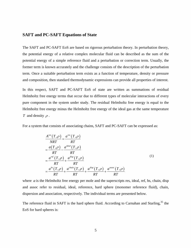
SAFT and PC-SAFT Equations of State

The SAFT and PC-SAFT EoS are based on rigorous perturbation theory. In perturbation theory,

the potential energy of a relative complex molecular fluid can be described as the sum of the

potential energy of a simple reference fluid and a perturbation or correction term. Usually, the

former term is known accurately and the challenge consists of the description of the perturbation

term. Once a suitable perturbation term exists as a function of temperature, density or pressure

and composition, then standard thermodynamic expressions can provide all properties of interest.

In this respect, SAFT and PC-SAFT EoS of state are written as summations of residual

Helmholtz free energy terms that occur due to different types of molecular interactions of every

pure component in the system under study. The residual Helmholtz free energy is equal to the

Helmholtz free energy minus the Helmholtz free energy of the ideal gas at the same temperature

T and density ρ .

For a system that consists of associating chains, SAFT and PC-SAFT can be expressed as:

( ) ( )

( ) ( )

( ) ( )

( ) ( ) ( ) ( )

, ,

, ,

, ,

, , , ,

res res

ideal

ref disp

hs chain disp assoc

A T a TNRT RT

a T a TRT RT

a T a TRT RT

a T a T a T a TRT RT RT RT

ρ ρ

ρ ρ

ρ ρ

ρ ρ ρ ρ

=

= −

= +

= + + +

(1)

where a is the Helmholtz free energy per mole and the superscripts res, ideal, ref, hs, chain, disp

and assoc refer to residual, ideal, reference, hard sphere (monomer reference fluid), chain,

dispersion and association, respectively. The individual terms are presented below.

The reference fluid in SAFT is the hard sphere fluid. According to Carnahan and Starling,35 the

EoS for hard spheres is:

6

( )22

134ηηη

−−

= mRTahs

(2)

where m is the number of spherical segments in each molecule and η is the reduced density that

can be calculated by the expression

omvρη 74048.0= (3)

In this expression, ov is the close-packed hard-core volume of the fluid which is evaluated using

the temperature-independent soft-core volume, oov , from the equation:

3

3exp1

−−=

kTuCvv

oooo (4)

which has been proposed by Huang and Radosz20.

In Eq. 4, kTuo

is the dispersion energy parameter per segment and C is a constant equal to 0.12

(the only deviating compound is hydrogen, for which the value is 0.241).

The interactions for the formation of chains from the monomer hard spheres are modelled

according to the equation:

( )( )31

5.01ln1ηη

−−

−= mRT

achain

(5)

which is based on Wertheim’s TPT1.

To account for the dispersion forces between the chains, the Alder36 equation based on molecular

simulation of the square-well fluid is used:

∑∑= =

=

4

1

9

1 74048.0i j

ji

ij

disp

kTuDm

RTa η (6)

where ijD are universal constants and:

+=

kTe

ku

ku o

1 (7)

7

where ek

is an energy parameter with constant value for most of the molecules with the

exception of some gases.20 The three parameters, m , oov and k

uo

, are regressed for every

component using experimental data for vapor pressure and saturated liquid density.

The difference between SAFT and PC-SAFT stems from the reference fluid used. In PC-SAFT,

the hard chain fluid is chosen over hard sphere. Consequently, the dispersion term in PC-SAFT

EoS is:

( ) ( )2 3 2 2 31 1 22 , ,

dispa I n m m mC I n m mRT

πρ εσ πρ ε σ= − − (8)

where

1

1 1−

∂∂

++=ρ

ρhc

hc ZZC (9)

and hcZ is the compressibility factor of hard chains. Furthermore,

( ) ( )∑=

=6

01 ,

i

ii nmamnI (10)

( ) ( )∑=

=6

02 ,

i

ii nmbmnI (11)

where ia and ib are functions of the chain length and:

( ) iiii am

mm

mam

mama 210211 −−

+−

+= (12)

( ) iiii bm

mm

mbm

mbmb 210211 −−

+−

+= (13)

The association term has its roots to Wertheim’s TPT1 and the expression for it is:

∑ ∑

+

−=

i Ai

AA

i

assoc

i

ii MXXx

RTa

21

2ln (14)

8

where iM is the number of association sites per molecule of species i and iAX is the fraction of

molecules of species i that are not hydrogen bonded at site A .The latter can be calculated by a

mass balance that results in:

1

1−

∆+= ∑∑

j B

BABj

A

j

jiji XX ρ (15)

In this equation jρ is the molar density of component j , while jiBA∆ is the strength of the bond

between two sites A and B , that belong to different molecules i and j .

The expression for the calculation of hydrogen bond strength is:

( )

−

=∆ 1exp3

kTdgd

jijiji

BABAseg

ijijijBA εκ (16)

where i jA Bε is the bonding (or association) energy, ji BAκ is the bonding volume and

( )jjiiij ddd +=21 is the average segment diameter.

In this work, the components under consideration were modelled as chain molecules exhibiting

the various interactions discussed above. Associating interactions were taken into account

between H2O molecules and between H2S molecules. More details on the association scheme of

H2O and H2S is provided later on.

Since the equations of SAFT and PC-SAFT are written in terms of the Helmholtz free energy,

they can be used to produce analytical equations for the evaluation of derivative properties.

Hence, by taking the derivative functions of the Helmholtz energy with respect to appropriate

variables, one can have the expressions for the derivative properties. For the association term, the

formalism of Michelsen and Hendriks37 was used, that results in analytic expressions and thus

reduce computational time substantially compared to the original expressions that require a trial-

and-error approach. More specifically, the following derivative properties are examined here:

Thermal expansion coefficient v

T TPk

∂∂

=α (17)

9

Isothermal compressibility coefficient T

TPk

∂∂

=−

ρρ1 (18)

Isochoric heat capacity 2

2vv

aC TT

∂= − ∂

(19)

Isobaric heat capacity ρα

Tvp k

TCC2

+= (20)

Joule-Thomson coefficient Tv

PTPT

∂∂

−

∂∂

=ρ

ρµ (21)

Speed of sound Tv

p PCC

∂∂

=ρ

ω (22)

10

Results and Discussion

Pure component parameters were fitted to experimental vapor pressure and saturated liquid

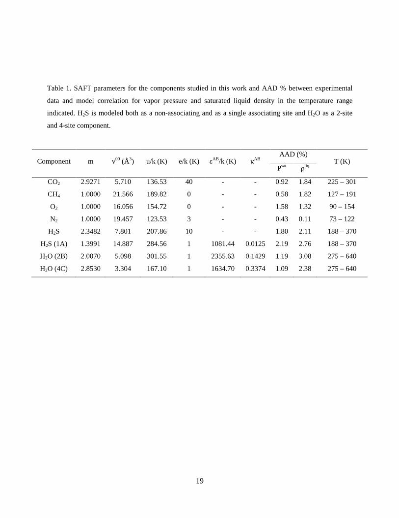
density data taken from NIST38. In Tables 1 and 2, the parameters for SAFT and PC-SAFT are

provided together with the percentage average absolute deviation (AAD %) between

experimental data and model calculations. Parameter m refers to the number of spherical

segments per molecule, with 1=m corresponding to a spherical molecule. In this case, SAFT

and PC-SAFT are expected to provide very similar results. In practice, m is one of the model

parameters fitted to experimental vapor pressure and saturated liquid density data and its

optimum value is larger than one.

Very good correlation of the vapor pressure and liquid density is obtained in all cases.

Calculation of liquid and vapor phase thermodynamic properties were performed for all

components in the temperature range 80 – 695 K and pressures up to 20 MPa, and compared

with experimental data.

Results for the accuracy of the two models to correlate the CO2 density at subcritical and

supercritical conditions are presented in Figure 1. As a first observation, the critical region is the

least accurate correlated by both EoS. PC-SAFT provides the relatively best prediction of the

critical point with Tc = 309.5 K and Pc = 7.92 MPa, while for SAFT it is: Tc = 315.5 K and Pc =

9.09 MPa. The experimental values are Tc = 304.13 K and Pc = 7.3773 MPa. This is also in

agreement with the more accurate prediction of the vapor pressure by PC-SAFT compared to

SAFT. The increasing inaccuracy in the critical region, due to the fact that both models are

mean-field theories that do not account for critical fluctuations, is also the main reason for the

high deviations between experimental data and model predictions for the derivative properties, as

it will be explained next. Away from the critical region, both at subcritical and supercritical

conditions, calculations are in very good agreement with the experimental data.

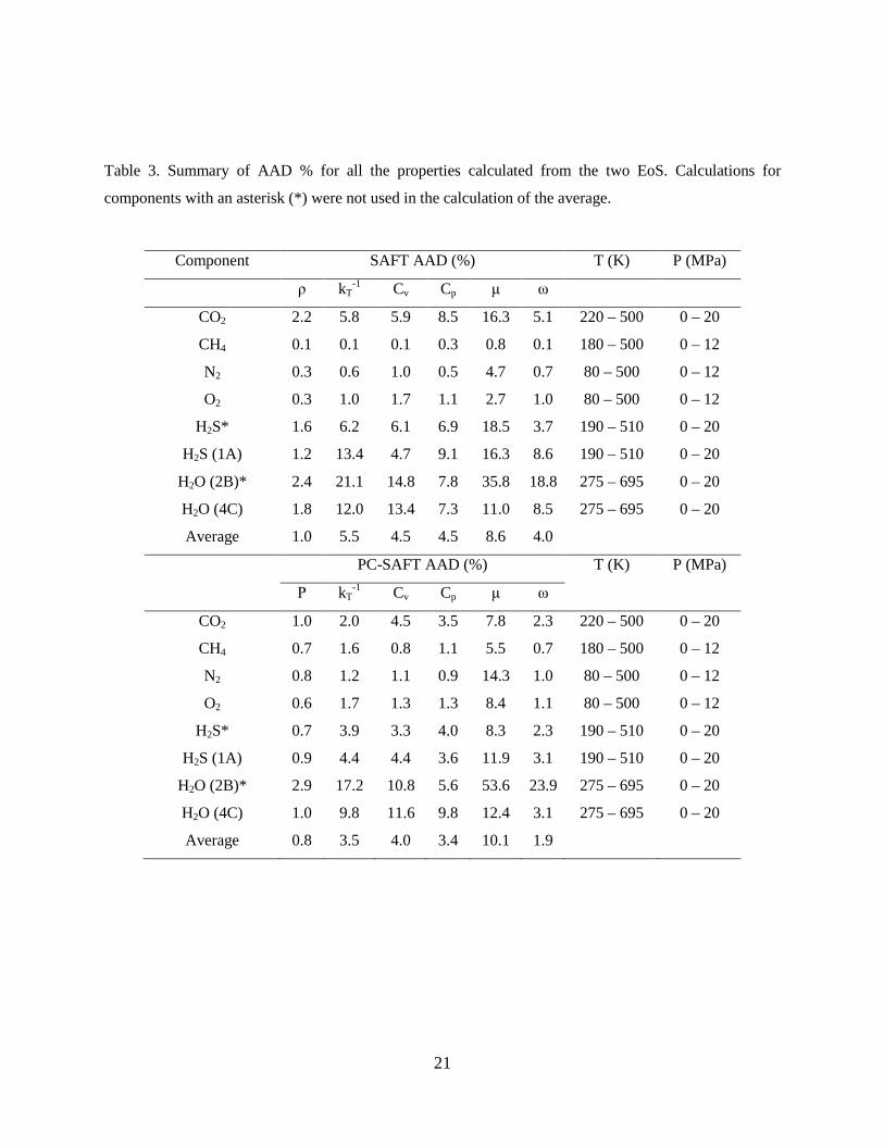
In Table 3, a summary of the AAD % between experimental data and EoS predictions for the

various properties of all the components examined is provided. On the average, PC-SAFT

performs systematically better than SAFT for all the properties, except for the Joule-Thomson

11

coefficient. In Figures 2 and 3, error contours of SAFT and PC-SAFT EoS predictions are shown

for pC , speed of sound, Joule-Thomson coefficient and isothermal compressibility coefficient of

CO2. The pC is well described by both equations, but PC-SAFT is giving lower errors. For the

calculation of heat capacities, the ideal gas contribution of the fluid is obtained from the NIST

database38 and the residual contribution from the EoS. The locus of the extreme values of pC

close to the critical point is well reproduced, but the values calculated from SAFT are quite

higher than the experimental. The accuracy of the calculations of pC by the two EoS in this work

is an improvement compared to earlier works based on a lattice EoS39 and a cubic EoS40.

Calculations for vC from both EoS are within less than 5 % from experimental data for most

gases, with an increasing deviation as the critical point is approached. The picture, however,

reverts if one focuses on the residual part of vC (Figure 4 and Table 4). Both models are in

qualitative agreement with experimental data, only. In the vicinity of the critical point, the

deviation increases and experimental data predict an increase in resvC as a function of

temperature while both SAFT and PC-SAFT predict the opposite trend. Such failure has been

reported also by Llovell et al.29, 33 for other fluids with the soft-SAFT EoS.

The pC of CO2 for a single isobar (12 MPa) was studied further in order to identify the effect of

residual over the ideal part of the property and the overall accuracy of the models. Calculations

and experimental data are presented in Figure 5. Although both models predict experimental data

with reasonable accuracy, PC-SAFT is much more accurate over the entire temperature range. In

liquid and near-critical conditions, the residual contribution is significant but at high

temperatures it becomes less important.

Calculations for the speed of sound are very accurate for both EoS. PC-SAFT deviates from

experimental data at most by 3.1 %, while SAFT performs slightly worse (AAD < 8.6 %), as it

can be seen in Table 3. From Eq. 22, one can see that ω depends on pC , vC and T

P

∂∂ρ

.

Consequently, one can argue that there is some cancellation of errors in the ratio of the two heat

capacities and the error in ω is mainly governed by the error in T

P

∂∂ρ

.

12

The Joule-Thomson coefficient is the least accurately predicted property from all properties

examined here. The overall AAD rises to 8.6 % for SAFT and 10.1 % for PC-SAFT (Table 3),

something that can be explained based on the fact that the Joule-Thomson coefficient depends on

two partial derivatives, as it can be seen in Eq. 21 so the error is probably additive. The error is

higher close to the points of phase change. At those points, the Joule-Thomson coefficient value

changes from negative to very high positive, in a very narrow temperature range. The reason for

this inaccuracy may lie in the fact that in those regions there are also abrupt changes in density.

This is why, while the pressure increases, the error in Joule-Thomson coefficient decreases, as

the density curves become smoother. It is important also to note that for the light gases (CH4, N2

and O2), PC-SAFT is significantly less accurate than SAFT for the prediction of Joule-Thomson

coefficient.

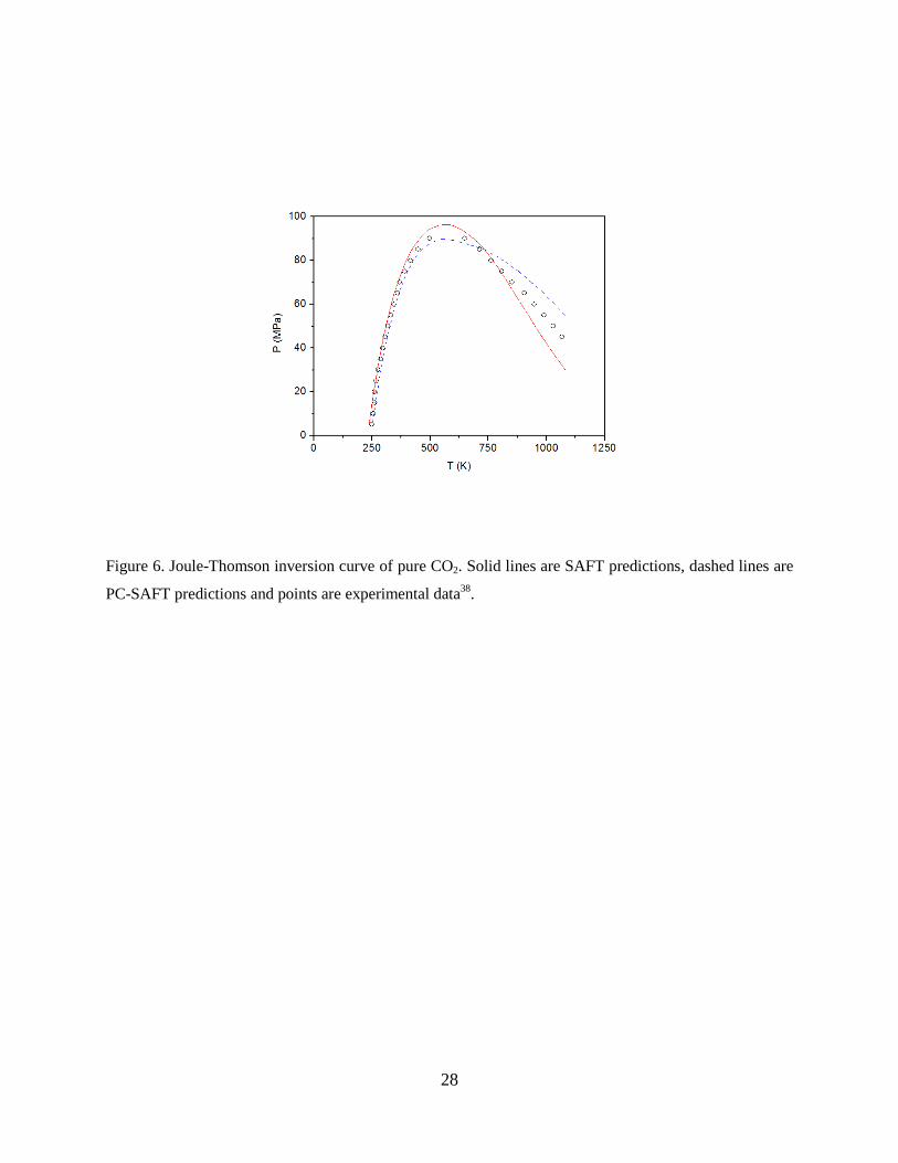
The Joule-Thomson inversion curve is an important property for fluids and refers to the

conditions where the Joule-Thomson coefficient is zero. The Joule-Thomson inversion curve of

CO2 is presented in Figure 6, and it can be seen that the two equations perform reasonably well

over the entire temperature examined.

The last derivative property examined is the isothermal compressibility coefficient, 1−Tk . Here

also, the agreement of the predictions with the experimental data is very good away from the

critical point and coexistence curve, because again, the fluctuations of density cause error in the

calculation of T

P

∂∂ρ

which is used for the calculation of 1−Tk .

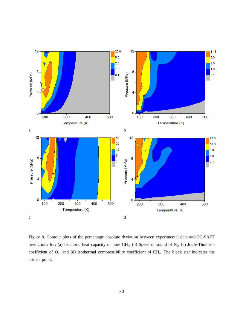
For O2, N2 and CH4, contour plots for the percentage absolute deviation experimental data and

model predictions for representative properties are presented in Figures 7 and 8. In general, the

accuracy of the model follows the pattern observed for CO2, so it decreases close to the critical

point and the coexistence curve. The property less accurately predicted is again the Joule-

Thomson coefficient. Overall, the properties of three non-polar, spherical molecules O2, N2 and

CH4 can be modelled by SAFT and PC-SAFT with high accuracy.

The accuracy of SAFT-based EoS for the prediction of derivative properties of pure fluids has

been thoroughly evaluated by Vega and co-workers29, 33, 34, 41 using Soft-SAFT and by Lafitte et

al.31, 42 using SAFT-VR EoS. The former work focused on n-alkanes, n-alkenes and 1-alcohols

13

and their mixtures at subcritical and supercritical conditions while the latter work concentrated

on 1-alcohols and 1-alcohol – n-alkane mixtures42 and n-alkanes31. A direct numerical

comparison between calculations with these other SAFT models and calculations presented here

is limited since the fluids and conditions examined are not the same. For the case of CH4, Llovell

and Vega29 reported an AAD % of 1.82 – 3.11 for the speed of sound, 14.9 – 25.3 for Cv and 3.2

– 9.7 for Cp at supercritical conditions (210 – 286 K), while our predictions result in a much

lower % AAD for all three properties.

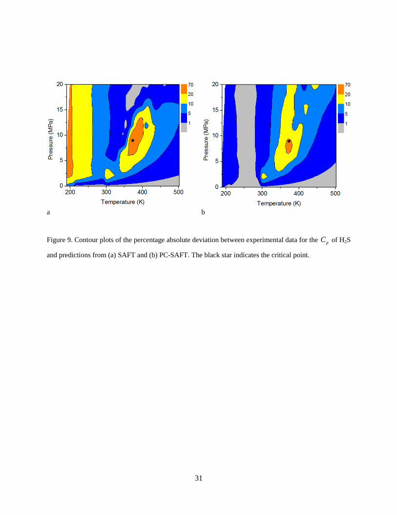
The last part of the analysis refers to explicit account for hydrogen bonding in H2S and H2O.

Experimental43 and literature data44 indicate that H2S form dimers through hydrogen bonding,

thus the one associating site model (1A) proves suitable in this case. However, calculations with

the 2 and 4 site models were also performed to explore the accuracy of these other schemes.

Calculations of derivative properties with 2 and 4 associating sites were significantly less

accurate than calculations using the 1 site model and so only these latter calculations are

presented here. The relevant parameters are presented in Tables 1 and 2. The associating model

improves only the correlation of saturated liquid density with PC-SAFT while higher deviations

are observed for the vapor pressure (both models) and saturated liquid density correlation with

SAFT. Similarly, explicit account of association results in marginal improvement of the

correlation of some of H2S derivative properties over the non-associating model. An indicative

graph in Figure 9 shows the AAD % of the total pC of pure H2S against the experimental data,

by using the 1-site model both in SAFT and PC-SAFT.

For modelling H2O, the popular 4 associating site model (4C) was used that corresponds to two

proton donor and two proton acceptor sites. To a first approximation, this is a physically realistic

model. However, it does not account for secondary effects such as three-body interactions, etc.

Consequently, an attempt was made to use a different associating scheme for H2O by assuming a

proton donor and a proton acceptor site (2B scheme in SAFT terminology). This is a model used

for 1-alcohols, although it is often applied for water, as well. Differences between the 2B and 4C

association sites are mainly observed in the prediction of derivative properties with SAFT.

Cleary, 4C provides lower error in the calculation of vapour pressure and saturated liquid density

(Tables 1 and 2) but also it improves the accuracy of the derivative properties as it can be seen in

Table 3.

14

By comparing the accuracy of the models for the various fluids, it becomes clear that for almost

all derivative properties, the highest % AAD between experimental data and model predictions

corresponds to H2O. It should be emphasized here that several other parameter sets provided

good correlation of the H2O phase equilibrium, but failed to predict accurately the derivative

properties. For example, deviations of up to 40% were obtained for pC . Consequently,

prediction of the derivative properties can be used as an additional test for pure component

parameters.

In Figure 10, contour plots for the percentage absolute deviation for pC of H2O are presented.

Clearly, the 4-site PC-SAFT model results in much more accurate prediction compared to the 4-

site SAFT model for the liquid phase properties. However, higher deviations are observed for the

vapor phase heat capacity, so that the overall errors from the two models are comparable, as

shown in Table 3. Finally, it is known experimentally that the pC of liquid water H2O goes

through a minimum at constant pressure. At 10 MPa for example, the experimental minimum

occurs at 301.5 K and has a value of 74.831 KmolJ ⋅/ . Calculations with SAFT revealed no

minimum value, while PC-SAFT predicted a minimum pC of 71.581 KmolJ ⋅/ at 367.7 K.

15

Conclusions

SAFT and PC-SAFT equations of state were applied to six fluids that are of interest to the CCS

technology. Their performance was evaluated for the correlation of vapor pressure and saturated

liquid density and for the prediction of second derivative thermodynamic properties in a wide

range of conditions.

The parameters used for both equations were fitted to VLE data (vapor pressure and liquid

density), and subsequently used to predict the second derivative properties accurately, giving low

errors, especially away from the critical point. From a physical point of view, as well as

applicability in engineering cases, it is important that a single set of parameters can be used for

both volumetric and derivative properties. PC-SAFT is shown to be more accurate than SAFT

for CO2 and H2S, while for the smaller molecules of O2, N2 and CH4, SAFT accuracy is

comparable, if not better, to that of PC-SAFT. For spherical molecules (m = 1), PC-SAFT has no

advantage over SAFT, as one might expect based on the formulation of the two theories.

Especially for the associating compounds under investigation, namely H2S and H2O, some very

useful conclusions stem from this study. Taking into account the hydrogen bonding of H2S does

not improve the performance of the models in the correlation of vapor pressure and the

prediction of derivative properties. For H2O, the 4-site associating model results in reasonably

good agreement with experimental data for both the SAFT and the PC-SAFT models for all

properties examined. In all cases, the Michelsen and Hendriks37 formulation was used for the

associating term that reduces computational time substantially.

The computation cost for the calculations presented here is low, since the derivative properties

from SAFT and PC-SAFT are calculated analytically. Thus, the models can be used reliably for a

CCS design.

16

Acknowledgements

The authors acknowledge financial support from the 7th European Commission Framework

Program for Research and Technological Development for project “Quantitative failure

consequence hazard assessment for next generation CO2 pipelines” (Project No.: 241346) and

from the Petroleum Institute Research Initiation Funding Program for project “An in-house

general-purpose simulator for multiscale multiphase flows in heterogeneous porous media for

enhanced oil recovery and carbon capture and storage processes”. Also, The Petroleum Institute

is acknowledged for a visiting PhD scholarship to NID.

17

References

1. Li, H.; Yan, J., Appl. Energy 2009, 86, 826-836. 2. Svensson, R.; Odenberger, M.; Johnsson, F.; Strömberg, L., Energ. Convers. Manage. 2004, 45, 2343-2353. 3. Forbes, S. M.; Verma, P.; Curry, T. E.; Friedmann, S. J.; Wade, S. M., CCS Guidelines: Guidelines for Carbon Dioxide Capture, Transport, and Storage. World Resources Institute 2008. 4. Zhang, Z. X.; Wang, G. X.; Massarotto, P.; Rudolph, V., Energ. Convers. Manage. 2006, 47, 702-715. 5. Mohitpour, M.; Golshan, H.; Murray, A., Pipeline Design & Construction: A Practical Approach. ASME Press 2007. 6. Li, H.; Yan, J., Appl. Energy 2009, 86, 2760-2770. 7. IPCC, IPCC Special Report: Carbon Dioxide Capture and Storage. A Special Report of Working Group III of the Intergovernmental Panel on Climate Change, 2005. 8. Lachet, V.; de Bruin, T.; Ungerer, P.; Coquelet, C.; Valtz, A.; Hasanov, V.; Lockwood, F.; Richon, D., Energy Procedia 2009, 1, 1641-1647. 9. Caubet, F., Z. kompr. Fluess. Gase Pressluft-Ind. 1904, 8, 65. 10. Bluemcke, A., Ann. Phys. Leipzig 1888, 34, 10-21. 11. Carroll, J. J., J. Can. Petrol. Technol. 2002, 41, 25-31. 12. Carroll, J. J.; Mather, A. E., J. Solution Chem. 1992, 21, 607-621. 13. Span, R.; Wagner, W., J. Phys. Chem. Ref. Data 1996, 25, 1509–1596. 14. Soave, G., Chem. Eng. Sci. 1972, 27, 1197-1203. 15. Peng, D.-Y.; Robinson, D. B., Ind. Eng. Chem. Fund. 1976, 15, 59-64. 16. Redlich, O.; Kwong, J. N. S., Chem. Rev. 1949, 44, 233-244. 17. Patel, N. C.; Teja, A. S., Chem. Eng. Sci. 1982, 37, 463-473. 18. Chapman, W. G.; Gubbins, K. E.; Jackson, G.; Radosz, M., Fluid Phase Equilibr. 1989, 52, 31-38. 19. Chapman, W. G.; Gubbins, K. E.; Jackson, G.; Radosz, M., Ind. Eng. Chem. Res. 1990, 29, 1709-1721. 20. Huang, S. H.; Radosz, M., Ind. Eng. Chem. Res. 1990, 29, 2284-2294. 21. Gross, J.; Sadowski, G., Ind. Eng. Chem. Res. 2001, 40, 1244-1260. 22. Wertheim, M. S., J. Stat. Phys. 1984, 35, 19-34. 23. Wertheim, M. S., J. Stat. Phys. 1984, 35, 35-47. 24. Wertheim, M. S., J. Stat. Phys. 1986, 42, 459-476. 25. Wertheim, M. S., J. Stat. Phys. 1986, 42, 477-492. 26. Economou, I. G., Ind. Eng. Chem. Res. 2001, 41, 953-962. 27. Müller, E. A.; Gubbins, K. E., Ind. Eng. Chem. Res. 2001, 40, 2193-2211. 28. Gregorowicz, J.; O'Connell, J. P.; Peters, C. J., Fluid Phase Equilibr. 1996, 116, 94-101. 29. Llovell, F.; Vega, L. F., J. Phys. Chem. B 2006, 110, 11427-11437. 30. Kortekaas, W. G.; Peters, C. J.; de Swaan Arons, J., Fluid Phase Equilibr. 1997, 139, 205-218. 31. Lafitte, T.; Bessieres, D.; Pineiro, M. M.; Daridon, J.-L., J. Chem. Phys. 2006, 124, 024509(1-16). 32. Llovell, F.; Vega, L. F., J. Phys. Chem. B 2005, 110, 1350-1362. 33. Llovell, F.; Peters, C. J.; Vega, L. F., Fluid Phase Equilibr. 2006, 248, 115-122. 34. Llovell, F.; Vega, L. F., J. Supercrit. Fluid. 2007, 41, 204-216. 35. Carnahan, N. F.; Starling, K. E., J. Chem. Phys. 1970, 53, 600-603. 36. Alder, B. J.; Young, D. A.; Mark, M. A., J. Chem. Phys. 1972, 56, 3013-3029.

18

37. Michelsen, M. L.; Hendriks, E. M., Fluid Phase Equilibr. 2001, 180, 165-174. 38. Lemmon, E. W.; Linden, M. O.; Friend, D. G., Thermophysical Properties of Fluid Systems. In NIST Chemistry WebBook, NIST Standard Reference Database Number 69, Linstrom, P. J.; Mallard, W. G., Eds. National Institute of Standards and Technology: Gaithersburg MD, 20899. 39. Lee, Y.; Shin, M. S.; Kim, H., J. Chem. Thermodyn. 2008, 40, 1580-1587. 40. Shin, M. S.; Lee, Y.; Kim, H., J. Chem. Thermodyn. 2007, 40, 688-694. 41. Dias, A. M. A.; Llovell, F.; Coutinho, J. A. P.; Marrucho, I. M.; Vega, L. F., Fluid Phase Equilibr. 2009, 286, 134-143. 42. Lafitte, T.; Piñeiro, M. M.; Daridon, J.-L.; Bessières, D., J. Phys. Chem. B 2007, 111, 3447-3461. 43. Lowder, J. E.; Kennedy, L. A.; Sulzmann, K. G. P.; Penner, S. S., J. Quant. Spectrosc. Ra. 1970, 10, 17-23. 44. Desiraju, G. R.; Steiner, T., The weak hydrogen bond in structural chemistry and biology. Oxford University Press Inc.1999.

19

Table 1. SAFT parameters for the components studied in this work and AAD % between experimental

data and model correlation for vapor pressure and saturated liquid density in the temperature range

indicated. H2S is modeled both as a non-associating and as a single associating site and H2O as a 2-site

and 4-site component.

Component m v00 (Å3) u/k (K) e/k (K) εAB/k (K) κAB AAD (%)

T (K) Psat ρliq

CO2 2.9271 5.710 136.53 40 - - 0.92 1.84 225 – 301

CH4 1.0000 21.566 189.82 0 - - 0.58 1.82 127 – 191

O2 1.0000 16.056 154.72 0 - - 1.58 1.32 90 – 154

N2 1.0000 19.457 123.53 3 - - 0.43 0.11 73 – 122

H2S 2.3482 7.801 207.86 10 - - 1.80 2.11 188 – 370

H2S (1A) 1.3991 14.887 284.56 1 1081.44 0.0125 2.19 2.76 188 – 370

H2O (2B) 2.0070 5.098 301.55 1 2355.63 0.1429 1.19 3.08 275 – 640

H2O (4C) 2.8530 3.304 167.10 1 1634.70 0.3374 1.09 2.38 275 – 640

20

Table 2. PC-SAFT parameters for the components studied in this work and AAD % between experimental

data and model correlation for vapor pressure and saturated liquid density in the temperature range

indicated. H2S is modeled both as a non-associating and as a single associating site and H2O as a 2-site

and 4-site component.

Component m σ (Å) ε/k (K) εAB/k (K) κAB AAD (%)

T (K) Psat ρliq

CO2 2.6037 2.555 151.04 - - 0.49 0.83 217 – 301

CH4 1.0000 3.704 150.03 - - 0.33 1.40 127 – 191

O2 1.1217 3.210 114.96 - - 0.34 1.80 90 – 154

N2 1.2053 3.313 90.96 - - 0.14 1.92 73 – 122

H2S 1.7163 3.009 224.96 - - 0.38 1.90 188 – 370

H2S (1A) 1.4183 3.243 245.49 735.07 0.0111 0.63 0.41 188 – 370

H2O (2B) 1.9599 2.362 279.42 2059.28 0.1750 1.18 3.92 275 – 640

H2O (4C) 2.1945 2.229 141.66 1804.17 0.2039 1.98 0.83 275 – 640

21

Table 3. Summary of AAD % for all the properties calculated from the two EoS. Calculations for

components with an asterisk (*) were not used in the calculation of the average.

Component SAFT AAD (%) T (K) P (MPa)

ρ kT

-1 Cv Cp μ ω

CO2 2.2 5.8 5.9 8.5 16.3 5.1 220 – 500 0 – 20

CH4 0.1 0.1 0.1 0.3 0.8 0.1 180 – 500 0 – 12

N2 0.3 0.6 1.0 0.5 4.7 0.7 80 – 500 0 – 12

O2 0.3 1.0 1.7 1.1 2.7 1.0 80 – 500 0 – 12

H2S* 1.6 6.2 6.1 6.9 18.5 3.7 190 – 510 0 – 20

H2S (1A) 1.2 13.4 4.7 9.1 16.3 8.6 190 – 510 0 – 20

H2O (2B)* 2.4 21.1 14.8 7.8 35.8 18.8 275 – 695 0 – 20

H2O (4C) 1.8 12.0 13.4 7.3 11.0 8.5 275 – 695 0 – 20

Average 1.0 5.5 4.5 4.5 8.6 4.0

PC-SAFT AAD (%) T (K) P (MPa)

Ρ kT

-1 Cv Cp μ ω

CO2 1.0 2.0 4.5 3.5 7.8 2.3 220 – 500 0 – 20

CH4 0.7 1.6 0.8 1.1 5.5 0.7 180 – 500 0 – 12

N2 0.8 1.2 1.1 0.9 14.3 1.0 80 – 500 0 – 12

O2 0.6 1.7 1.3 1.3 8.4 1.1 80 – 500 0 – 12

H2S* 0.7 3.9 3.3 4.0 8.3 2.3 190 – 510 0 – 20

H2S (1A) 0.9 4.4 4.4 3.6 11.9 3.1 190 – 510 0 – 20

H2O (2B)* 2.9 17.2 10.8 5.6 53.6 23.9 275 – 695 0 – 20

H2O (4C) 1.0 9.8 11.6 9.8 12.4 3.1 275 – 695 0 – 20

Average 0.8 3.5 4.0 3.4 10.1 1.9

22

Table 4. Summary of AAD % for Cvres of CO2 calculated from the two EoS for T = 220 – 500 K.

Cvres AAD %

P (MPa) SAFT PC-SAFT 0.1 61.8 50.7 1 60.7 47.0 2 65.8 43.5 5 49.6 38.9 8 46.2 38.7

10 44.5 38.7 12 41.7 37.7 15 38.0 36.2 20 30.8 35.5

Average 48.8 40.8

23

Figure 1. Contour plots of the percentage absolute deviation between experimental data and SAFT

predictions (left) and PC-SAFT predictions (right) for the density of pure CO2. The black star indicates

the critical point.

24

a

b

c

d

Figure 2. Contour plots of the percentage absolute deviation between experimental data of pure CO2 and

SAFT predictions for: (a) pC , (b) Speed of sound, (c) Joule-Thomson coefficient and (d) Isothermal

compressibility coefficient. The black star indicates the critical point.

25

a

b

c

d

Figure 3. Contour plots of the percentage absolute deviation between experimental data of pure CO2 and

PC-SAFT predictions for: (a) pC , (b) Speed of sound, (c) Joule-Thomson coefficient and (d) Isothermal

compressibility coefficient. The black star indicates the critical point.

26

a

b

Figure 4. Residual isochoric heat capacity of pure CO2 for (a) subcritical and (b) supercritical regime.

Solid lines are SAFT predictions, dashed lines are PC-SAFT predictions and points are experimental

data.38

27

Figure 5. pC of CO2 at 12MPa. Experimental data from NIST, ideal gas contribution, SAFT and PC-SAFT predictions.

28

Figure 6. Joule-Thomson inversion curve of pure CO2. Solid lines are SAFT predictions, dashed lines are

PC-SAFT predictions and points are experimental data38.

29

a

b

c

d

Figure 7. Contour plots of the percentage absolute deviation between experimental data and SAFT

predictions for: (a) Isochoric heat capacity of pure CH4, (b) Speed of sound of N2, (c) Joule-Thomson

coefficient of O2, and (d) isothermal compressibility coefficient of CH4. The black star indicates the

critical point.

30

a

b

c

d

Figure 8. Contour plots of the percentage absolute deviation between experimental data and PC-SAFT

predictions for: (a) Isochoric heat capacity of pure CH4, (b) Speed of sound of N2, (c) Joule-Thomson

coefficient of O2, and (d) isothermal compressibility coefficient of CH4. The black star indicates the

critical point.

31

a

b

Figure 9. Contour plots of the percentage absolute deviation between experimental data for the pC of H2S

and predictions from (a) SAFT and (b) PC-SAFT. The black star indicates the critical point.

32

a

b

Figure 10. Contour plots of the percentage absolute deviation between experimental data for pC of H2O

and predictions from (a) SAFT and (b) PC-SAFT. The black star indicates the critical point.