evaluation of two prototype three phase photovoltaic water
TRANSCRIPT

Univers
ity of
Cap
e Tow
n
Evaluation of two prototype three phase photovoltaic water pumping systems
Axel Scholle B.Sc (Eng) UCT
Submitted to the University of Cape Town in partial fulfilment for the degree of Master of Science tn Engineering
Energy for Development Research Centre Energy Research Institute, University of Cape Town
May 1994
.-.Al.-.!-.1-•"·~,.,...,,._,.:_,,\c:·:>.·::..••~··~·:..-tq.;.'t"il•:f!'-·':" .; ·; ~.: -~"rt,t...~
The University cf Cape Town h1-1s been g;ven :; the right to. rer:irr:duce this. thesis in v1ha!e ;
or In part. c:~::~: .. ~:~ ::~~~:~.,,3,~::~.1

Univers
ity of
Cap
e Tow
n
The copyright of this thesis vests in the author. No quotation from it or information derived from it is to be published without full acknowledgement of the source. The thesis is to be used for private study or non-commercial research purposes only.
Published by the University of Cape Town (UCT) in terms of the non-exclusive license granted to UCT by the author.

Univers
ity of
Cap
e Tow
n
ABSTRACT
·Two prototype three phase AC photovoltaic pump systems (Solvo, ML T) and a DC PV pump (Miltek) were tested on a farm borehole in Namibia (latitude 21°6', longitude 17°6'). The PV array consisted of twelve modules (636Wpeak) mounted on a singleaxis passive tracker. The depth of the water was 75m and a progressive cavity pump with a self-compensating stator was used in all the tests. Customised data acquisition was designed to measure performance characteristics through a range of operating conditions (mainly steady state); a secondary data acquisition system was used to capture samples of high frequency signals. The data allowed detailed analysis of system, subsystem and component performance, as well as performance evaluation over Standard Solar Days.
The focus of the investigation was evaluation of the AC prototypes, in terms of performance, other technical factors, reliability and economic criteria. The analogbased DC system served as a basis for comparison.
Both AC systems employed microprocessor control and PWM variable-frequency variable-voltage inversion. Efficiencies, optimality, stability, start-up behaviour, nonproductive operating modes and protection were examined. A number of recommendations were proposed for improvements in the basic control algorithms, monitoring and managing non-productive modes, improved protection, layout and user diagnostic features.
AC PV pumping systems are less common than DC counterparts, in the application and power range investigated. AC systems are potentially cheaper, and the inverters and motors can be manufactured locally. The tested prototypes did not attain subsystem or system efficiencies equal to the DC PV pump, but with optimisation could still provide an attractive alternative. Simulations were conducted (using typical meteorological year data, for two sites) for the tested systems, and additionally for a proven Grundfos AC system with centrifugal pump. The results indicated lowest unit pumped water costs for the DC system, followed by the prototype AC systems, for pumping at a 75m head in the sub-kW power range. ~

Univers
ity of
Cap
e Tow
n
ACKNOWLEDGEMENTS
It has been some time now and it was not without help. I am thanking - -
Bill Cowan, my supervisor, for excellent and sensitive supervision - I enjoyed our interaction;
John Greene, my co-supervisor for his guidance in design of the measurement electronics;
Conrad Roedern, who financed this project; Herzlichen Dank Conrad, fur Zeit, Fuhrung, Gedanken und Geduld; Thank you Solar Age Namibia;
Glynn Morris for his efforts to arrange this project with Conrad and help me on my way towards monitoring;
Mark Davis for software support. And thanks especially for that help in those last hours;
Jochen Roeber for the time taken to explain things about power measurement; Helmut Geiger, Rudi Wortmann and Erwin Trossbach van Elwiwa fOr Hilfsbereitschaft Eberhart Fischer and Peter Toll van Edelstahlbau fOr eine nette Anzahl
Metalstrukturen Andreas and Mandy Bruckner for making a room available to me for such a really long
time - I felt comfortable with you; Marco und Wiltrud Simoni fOr Unterhaltung, Hilfe, schones Essen und enorme Pilze -
herzlichen Dank, daB lhr mich so lange untergebracht habt; Rudi und Giesel Allers fur den Gebrauch Eures Wohnwagens - dies hat das Dasein
auf der Farm praktsich, genial und romantisch gemacht; Gero Diekmann, hab' Dank Gero, mein Freund, dafur daB Du mir das Auto zur
Verfugung gestellt hast; Pari Callias for organising things at EDRC while I was in Namibia; Chris Purcell for advice on measurements; Peter Beckedahl fur daB beistehen in manch einem Test; Stephanie Hardy for giving me lots of time and taking care of Pascoe - it was not
always easy but we did okay, for the rest lets not rely on words; , Marlies Scholle, Du standest voll dahinter und hast dabei sicher auch gelitten - daB
ist jetzt vorbei - vielen Dank fur Deine Unterstotzung; Renate Scholle, als Retter in jeder Not - Bruderchen bedankt sich.

Univers
ity of
Cap
e Tow
n
TABLE OF CONTENTS
Abstract ...................................................... .
Acknowledgements . . . . . . . . . . . . . . . . . . . . . . . . . . . . . . . . . . . . . . . . . . . . . . . . m
List of Figures . . . . . . . . . . . . . . . . . . . . . . . . . . . . . . . . . . . . . . . . . . . . . . . . . . . xm
List of Tables XIX
Abbreviations . . . . . . . . . . . . . . . . . . . . . . . . . . . . . . . . . . . . . . . . . . . . . . . . . . . xx1
List of symbols . . . . . . . . . . . . . . . . . . . . . . . . . . . . . . . . . . . . . . . . . . . . . . . . . . xxm
Chapter One: Introduction . . . . . . . . . . . . . . . . . . . . . . . . . . . . . . . . . . . 1 1.1 Conventions for this dissertation ................... ·. . . . . . . . 1 1.2 Objectives . . . . . . . . . . . . . . . . . . . . . . . . . . . . . . . . . . . . . . . . . . . 2 1.3 Scope . . . . . . . . . . . . . . . . . . . . .. . . . . . . . . . . . . . . . . . . . . . . . . . 2 1.4 Structure . . . . . . . . . . . . . . . . . . . . . . . . . . . . . . . . . . . . . . . . . . . . 3 1 . 5 The evaluation criteria . . . . . . . . . . . . . . . . . . . . . . . . . . . . . . . . . . 3
Chapter Two: Photovoltaic water pumping . . . . . . . . . . . . . . . . . . . . . . 5 2.1 Advantages and disadvantages of PV pumping . . . . . . . . . . . . . . . . 5 2.2 PV pumping configurations . . . . . . . . . . . . . . . . . . . . . . . . . . . . . . . 6 2.3 Classifying the systems under test . . . . . . . . . . . . . . . . . . . . . . . . . . 9 2.4 Three phase PVP's versus DC PVP's . . . . . . . . . . . . . . . . . . . . . . . 11 2.5 Analog versus digital controller implementation . . . . . . . . . . . . . . . . . 11 2.6 Introduction to three phase PV pumps . . . . . . . . . . . . . . . . . . . . . . . 13
2.6.1 AC technical developments . . . . . . . . . . . . . . . . . . . . . . . . . . . 13 2.6.2 Switch-mode inverters . . . . . . . . . . . . . . . . . . . . . . . . . . . . . . . 13 2.6.3 The induction motors . . . . . . . . . . . . . . . . . . . . . . . . . . . . . . . . 21 2.6.4 Torque pulsations . . . . . . . . . . . . . . . . . . . . . . . . . . . . . . . . . . 25 2.6.5 The function of DC input capacitance . . . . . . . . . . . . . . . . . . . . 26 .
2.7 Efficiency considerations in PV pump systems· . . . . . . . . . . . . . . . . . 26 2.7.1 PV pump component efficiencies . . . . . . . . . . . . . . . . . . . . . . . 26 2.7.2 The impact of component interaction on the overall efficiency . . . 32

Univers
ity of
Cap
e Tow
n
v1 Table of contents
Chapter Three: System description ............................ . 3.1 Deitails of the site ..................................... . 3.2 The array ........... : ............................ :· ..
3.2.1 Specifications ................................. ; ... . 3.2.2 Configurations used ................................ . 3.2.3 Tracking array mechanism ........................... .
3.3 The pump .......................................... . 3.3.1 Specifications .................................... . 3.3.2 Installation ...................................... . 3.3.3 Transmission .................................. · ... .
3.4 The Miltek DC to DC converter ........................... . 3.4.1 Specifications .................................... . 3.4.2 Configuration of the converter in the PVP test system ....... . 3.4.3 Control algorithm .................................. . 3.4.4 Hardware ....................................... . 3.4.5 Signal profile ..................................... .
3.5 The Solve three phase inverter ........................... . 3.5.1 Specifications .................................. : .. 3.5.2 Configuration of the inverter in the PVP test system ......... . 3.5.3 Hardware ....................................... . 3.5.4 Software ........................................ . 3.5.5 Signal profile ..................................... . 3.5.6 Future developments .......... : .................... .
3.6 The1 ML T three phase inverter ............................ . 3.6.1 Specifications .................................... . 3.6.2 Configuration of the inverter in the PVP test system ......... . 3.6.3 Hardware ....................................... . 3.6.4 Software ........................................ . 3.6.5 Signal profile ..................................... .
3.7 The motors ......................................... . 3. 7. 1 Specifications of the Baldor DC motor ................... . 3.7.2 Specifications of the GEC three phase induction motor ....... .
Chapter Four: Research questions and test methodology .......... . 4.1 Research questions ................................... . 4.2 Choice of parameters .................................. .
4.2.1 Equations ....................................... . 4.2.2 Parameters ...................................... .
4.3 Test methodology ..................................... .
35 35 36 36 37 37 38 38 38 38 39 39 39 40 40 42 43 43 43 44 47 49 40 51 51 51 51 54 55 57 \
57 57
59 59 61 61 63 64

Univers
ity of
Cap
e Tow
n
Table of contents
Chapter Five: Data acquisition systems ........................ . 5.1 Description of the primary data acquisition system .. : ........... .
5.1.1 Transducers ..................................... . 5.1.2 Data logger ...................................... . 5.1.3 Signal interface ................................... . 5.1.4 Power meter ..................................... . 5.1.5 Design procedure for the signal processing units ........... .
· 5.1.6 Layout of the primary data acquisition system ............. . 5.1. 7 Limitations of the signal processing unit ................. . 5.1.8 Problems encountered .............................. .
5.2 Calibration .......................................... . 5.3 Uncertainty in the measured data ......................... . 5.4 The secondary data acquisition unit ........................ .
Chapter Six: Array, pump and Miltek system performance ......... . 6.1 Array performance evaluation ............................ .
6.1.1 Array ~haracteristics ........... : ................... . 6.1.2 Array efficiency compared to the specifications ............. . 6.1.3 Fixed voltage operation in relation to the MPP ............. . 6.1.4 The effect of shading on the IV curve ................... . 6.1.5 Tracking versus fixed array .......................... .
6.2 Pump performance. evaluation ............................. . 6.2.1 Flowrate anci'drawdown correlations to pump speed ........ . 6.2.2 Torque characteristics of the pump ..................... . 6.2.3 Characteristics of the pumping set at different heads ........ . 6.2.4 Pumping set losses ................................ . 6.2.5 Comparison to pump specifications ..................... . 6.2.6 Conclusion on the type of pump used ................... .
6.3 Miltek system performance analysis ......................... . 6.3.1 Converter and motor performance ..................... . 6.3.2 Array operating point characteristics .. : ................. . 6.3.3 General observations ............................... . 6.3.4 System performance ............................... .
i't(-'. '
.. Vll
67 67 69 72 73 73 75 75 76 77 79 81 82
83 83 83 85 87 89 90 93 94 96
101 102 103 106 107 108 111 113 114

Univers
ity of
Cap
e Tow
n
v111 Table of contents
Chapter S:even: Solvo system performance analysis . . . . . . . . . . . . . . . 119 7.1 Invert.er and motor performance . . . . . . . . . . . . . . . . . . . . . . . . . . . 121
7. 1 . 1 Efficiency at standard head . . . . . . . . . . . . . . . . . . . . . . . . . . . 121 7 .1.2 Efficiency at higher heads . . . . . . . . . . . . . . . . . . . . . . . . . . . . 124 7.1.3 Characteristic inverter and motor curves . . . . . . . . . . . . . . . . . . 125
7.2 Ste!ady state array operating point characteristics . . . . . . . . . . . . . . . 126 7.3 Dynamic array operating point characteristics . . . . . . . . . . . . . . . . . . 126
7. 3.1 Shape of oscillation waveform . . . . . . . . . . . . . . . . . . . . . . . . . 127 7 .3.2 Array power losses .......... , . . . . . . . . . . . . . . . . . . . . . . 127 7.3.3 PWM envelope . . . . . . . . . . . . . . . . . . . . . . . . . . . . . . . . . . . . 130 7 .3.4 Effects of increased input capacitance . . . . . . . . . . . . . . . . . . . . 130
7.4 Voltage to hertz relation . . . . . . . . . . . . . . . . . . . . . . . . . . . . . . . . . 131 7. 5 · Observed control algorithm characteristics . . . . . . . . . . . . . . . . . . . . 133 7 .6 General observations ... ·. . . . . . . . . . . . . . . . . . . . . . . . . . . . . . . . 135 7. 7 System performance . . . . . . . . . . . . . . . . . . . . . . . . . . . . . . . . . . . 138
7. 7 .1 Instantaneous performance . . . . . . . . . . . . . . . . . . . . . . . . . . . 138 7. 7 .2 Daily energy efficiency performance . . . . . . . . . . . . . . . . . . . . . 139
Chapter Eight: ML T system performance analysis . . . . . . . . . . . . . . . . . 143 8.1 lnv1erter and motor performance ...................... ~ . . . . . 144
8.1.1 Efficiency at standard head . . . . . . . . . . . . . . . . . . . . . . . . . . . 144 8.1.2 Efficiency at higher head . . . . . . . . . . . . . . . . . . . . . . . . . . . . . 148 8.1.3 Characteristic inverter and motor curves . . . . . . . . . . . . . . . . . . 149
8.2 Steady state array operating point characteristics .... '. . . . . . . . . . . 150 8.3 Dynamic array operating point characteristics . . . . . . . . . . . . . . . . . . 152
8.3.1 Shapes of oscillation waveform . . . . . . . . . . . . . . . . . . . . . . . . . 152 8.3.2 Array power losses . . . . . . . . . . . . . . . . . . . . . . . . . . . . . . . . . 153 8.3.3 PWM envelope ......................... " . . . . . . . . . . 154 8.3.4 Effects of increased input capacitance . . . . . . . . . . . . . . . . . . . . 155
8.4 Voltage to hertz relation . . . . . . . . . . . . . . . . . . . . . . . . . . . . . . . . . 157 8.5 Observed control algorithm characteristics . . . . . . . . . . . . . . . . . . . . 158
8.5.1 Basic control algorithm implementation . . . . . . . . . . . . . . . . . . . 158 8.5.2 Fixed voltage operation . . . . . . . . . . . . . . . . . . . . . . . . . . . . . . 158 8.5.3 Maximum speed tracking . . . . . . . . . . . . . . . . . . . . . . . . . . . . . 159
8.6 General observations . . . . . . . . . . . . . . . . . . . . . . . . . . . . . . . . . . . 161 8.7 System performance . . . . . . . . . . . . . . . . . . . . . . . . . . . . . . . . . . . 163
8.7.1 Instantaneous performance . . . . . . . . . . . . . . . . . . . . . . . . . . . 163 8. 7 .2 Daily energy efficiency performance . . . . . . . . . . . . . . . . . . . . . 165

Univers
ity of
Cap
e Tow
n
Table of contents 1x
Chapter Nine: Proposed improvements for the prototype inverters . . . . 171 9.1 Control algorithm evaluation ....................... · . . . . . . . 171 . 9.1.1 Problem analysis ........ ·. . . . . . . . . . . . . . . . . . . . . . . . . . . 172
9.1.2 Suggestions towards the design of a suitable controller · . . . . . . . 17 4 9.2 Monitoring of undesired states of operation . . . . . . . . . . . . . . . . . . . 179
9.2.1 Incorrect array operating point . . . . . . . . . . . . . . . . . . . . . . . . . 1. 79 9.2.2 Minimum power threshold . . . . . . . . . . . . . . . . . . . . . . . . . . . . 180 9.2.3 Monitoring overvoltage . . . . . . . . . . . . . . . . . . . . . . . . . . . . . . . 181
9.3 Voltage to hertz relation . . . . . . . . . . . . . . . . . . . . . . . . . . . . . . . . . 182 9.4 Solvo inverter switching frequency . . . . . . . . . . . . . . . . . . . . . . . . . . 183 9.5 Peculiarities of the ML T inverter ............ : . . . . . . . . . . . . . . 184 9.6 Inverter protection . . . . . . . . . . . . . . . . . . . . . . . . . . . . . . . . . . . . . 185 9. 7 General design considerations . . . . . . . . . . . . . . . . . . . . . . . . . . . . 189
Chapter Ten: Comparative evaluation and simulation . . . . . . . . . . . . . . 191 10.1 Performance of the Miltek, Solvo and ML T PVP systems . . . . . . . . . 191
10.1.1 Instantaneous performance . . . . . . . . . . . . . . . . . . . . . . . . . . 191 10.1.2 Daily energy efficiency performance .. : . . . . . . . . . . . . . . . . . 195
10.2 Simulated comparison with a Grundfos PVP system . . . . . . . . . . . . 199 10.3 Other technical aspects of the PVP systems . . . . . • . . . . . . . . . . . . 204
10.3.1 System requirements . . . . . . . . . . . . . . . . . . . . . . . . . . . . . . . 204 10.3.2 System attributes . . . . . . . . . . . . . . . . . . . . . . . . . . . . . . . . . . 206
10.4 Cost analysis . . . . . . . . . . . . . . . . . . . . . . . . . . . . . . . . . . . . . . . . 208
Chapter Eleven: Conclusions_ ................. : . . . . . . . . . . . . . . . 213
Chapter Twelve: References . . . . . . . . . . . . . . . . . . . . . . . . . . . . . . . . . . 221
APPENDIX A 1: PV pump component specification sheets . . . . . . . . . . . . . . 227 A 1.1 Siemens M55S module . . . . . . . . . . . . . . . . . . . . . . . . . . . . . . . . 227 A 1.2 Zomeworks TRPM 12/AR passive solar tracker . . . . . . . . . . . . . . . . 228 A 1.3 Mono S2M borehole pump . . . . . . . . . . . . . . . . . . . . . . . . . . . . . . 230 A 1.4 Salvo circuit breaker and power module . . . . . . . . . . . . . . . . . . . . 231
A 1.4.1 Thermal three phase circuit breaker Mbs 25 . . . . . . . . . . . . . . 231 A 1.4.2 IGBT module BSM 15 GD 100 D . . . . . . . . . . . . . . . . . . . . . . 232
A 1.5 GEC ?OW DZ90L three phase motor . . . . . . . . . . . . . . . . . . . . . . . 233
...

Univers
ity of
Cap
e Tow
n
x Tab/E~ of contents
APPENDIX A2: Test methodology details . . . . . . . . . . . . . . . . . . . . . . . . . . 235 A2.1 The array . . . . . . . . . . . . . . . . . . . . . . . . . . . . . . . . . . . . . . . . . . 235
A2.1.1 IV curves ....................................... 236 A2.1 . .2 Tracking versus fixed array . . . . . . . . . . . . . . . . . . . . . . . . . . 237
A2.2 The pump . . . . . . . . . . . . . . . . . . . . . . . . . . . . . . . . . . . . . . . . . . 238 A2.2.1 Correlations . . . . . . . . . . . . . . . . . . . . . . . . . . . . . . . . . . . . . 238 A2.2.2 Torque and efficiency characteristics . . . . . . . . . . . . . . . . . . . . 239 A2.2.3 Pump characteristics at higher heads . . . . . . . . . . . . . . . . . . . 239
A2.3 Tl1e Miltek DC system . . . . . . . . . . . . . . . . . . . . . . . . . . . . . . . . . 240 A2.3.1 The main system and component performance tests . . . . . . . . 240 A2.3.2 Dynamic array operating point with the Miltek converter . . . . . . 241 A2.3.3 Dynamic conditions . . . . . . . . . . . . . . . . . . . . . . . . . . . . . . . . 241
A2.4 Tile Salvo and ML T three phase systems . . . . . . . . . . . . . . . . . . . 242 A2.4.1 The main system and component performance tests . . . . . . . . 242 A2.4.2 Dynamic array operating point tests . . . . . . . . . . . . . . . . . . . . 243 A2.4. 3 Dynamic operating conditions test . . . . . . . . . . . . . . . . . . . . . . 244
APPENDIX. A3: Specifications for the data acquisition systems . . . . . . . . . . 245 A3.1 Transducers and data logger specification sheets . . . . . . . . . . . . . . 245
A3.1.1 Ll-COR pyranometer Ll-200SZ . . . . . . . . . . . . . . . . . . . . . . . . 245 A3.1.2 Temperature sensor LM35D . . . . . . . . . . . . . . . . . . . . . . . . . . 246 A3.1.3 LEM current probe LA 50-P . . . . . . . . . . . . . . . . . . . . . . . . . . 247 A3.1.4 Loadcell UBG 10 . . . . . . . . . . . . . . . . . . . . . . . . . . . . . . . . . . 248 A3.1.!5 Optical switch TCST 2000 . . . . . . . . . . . . . . . . . . . . . . . . . . . 249 A3.1.6 Flow-captor Type 4113.30 . . . . . . . . . . . . . . . . . . . . . . . . . . . 250 A3.1.~r PSM water meter size 3 . . . . . . . . . . . . . . . . . . . . . . . . . . . . . 251 A3.1.B Pressure transmitter model 891.14.525 . . . . . . . . . . . . . . . . . . 252 A3.1.B Data logger MS-256 . . . . . . . . . . . . . . . . . . . . . . . . . . . . . . . 253
A3.2 Interface circuits and description . . . . . . . . . . . . . . . . . . . . . . . . . . 254 A3.2. 'I lrradiance . . . . . . . . . . . . . . . . . . . . . . . . . . . . . . . . . . . . . . . 255 A3.2.2 Temperature . . . . . . . . . . . . . . . . . . . . . . . . . . . . . . . . . . . . . 256 A3.2.~~ Array voltage . . . . . . . . . . . . . . . . . . . . . . . . . . . . . . . . . . . . . 256 A3.2.4 Array current . . . . . . . . . . . . . . . . . . . . . . . . . . . . . . . . . . . . . 257 A3.2.E> Converter voltage . . . . . . . . . . . . . . . . . . . . . . . . . . . . . . . . . 258 A3.2.6 Converter current . . . . . . . . . . . . . . . . . . . . . . . . . . . . . . . . . 258 A3.2. 7' Motor torque . . . . . . . . . . . . . . . . . . . . . . . . . . . . . . . . . . . . . 259 A3.2.Ei Motor speed . . . . . . . . . . . . . . . . . . . . . . . . . . . . . . . . . . . . . 260 A3.2.9 Flowrate . . . . . . . . . . . . . . . . . . . . . . . . . . . . . . . . . . . . . . . . 260 A3.2.10 Static and pressure head . . . . . . . . . . . . . . . . . . . . . . . . . . . 260 A3.2.11 Power supply ......... : . . . . . . . . . . . . . . . . . . . . . . . . . 261
A3.3 Power meter circuits and description . . . . . . . . . . . . . . . . . . . . . . . 262 A3.3.1 Inverter current . . . . . . . . . . . . . . . . . . . . . . . . . . . . . . . . . . . 263 A3.3.2 Inverter frequency . . . . . . . . . . . . . . . . . . . . . . . . . . . . . . . . . 265 A3.3.3 Inverter voltage . . . . . . . . . . . . . . . . . . . . . . . . . . . . . . . . . . . 265 A3.3.4 Inverter active power . . . . . . . . . . . . . . . . . . . . . . . . . . . . . . . 268

Univers
ity of
Cap
e Tow
n
Table of contents XI
A3.3.S Power supply . . . . . . . . . . . . . . . . . . . . . . . . . . . . . . . . . . . . 270 A3.4 Data sheets for electronic components . . . . . . . . . . . . . . . . . . . . . 271 A3.S Specifications of calibration devices . . . . . . . . . . . . . . . . . . . . . . . . 277
A3.S.1 Ll-COR calibration certificate . . . . . . . . . . . . . . . . . . . . . . . . . 277 A3.S.2 Fluke 83 DVM . . . . . . . . . . . . . . . . . . . . . . . . . . . . . . . . . . . . . 277 A3.S.3 Soar DVM . . . . . . . . . . . . . . . . . . . . . . . . . . . . . . . . . . . . . . . 278
A3.6 Uncertainty analysis of acquired data . . . . . . . . . . . . . . . . . . . . . . 279 A3.6.1 Plane of array irradiance data . . . . . . . . . . . . . . . . . . . . . . . . . 282 A3.6.2 Ambient and module temperature . . . . . . . . . . . . . . . . . . . . . . 282 A3.6.3 Array voltage . . . . . . . . . . . . . . . . . . . . . . . . . . . . . . . . . . . . . 283 A3.6.4 Array current . . . . . . . . . . . . . . . . . . . . . . . . . . . . . . . . . . . . . 283 A3.6.S Converter voltage . . . . . . . . . . . . . . . . . . . . . . . . . . . . . . . . . 284 A3.6.6 Converter current . . . . . . . . . . . . . . . . . . . . . . . . . . . . . . . . . 284 A3.6. 7 Motor torque . . . . . . . . . . . . . . . . . . . . . . . . . . . . . . . . . . . . . 28S A3.6.8 Motor speed .. ·. . . . . . . . . . . . . . . . . . . . . . . . . . . . . . . . . . . 28S A3.6.9 Flowrate . . . . . . . . . . . . . . . . . . . . . . . . . . . . . . . . . . . . . . . . 286 A3.6.1 O Static head ........ ·. . . . . . . . . . . . . . . . . . . . . . . . . . . . . 286 A3.6.11 Inverter current . . . . . . . . . . . . . . . . . . . . . . . . . . . . . . . . . . 287 A3.6.12 Inverter frequency . . . . . . . . . . . . . . . . . . . . . . . . . . . . . . . . 287 A3.6.13 Inverter voltage . . . . . . . . . . . . . . . . . . . . . . . . . . . . . . . . . . 288 A3.6.14 Inverter power . . . . . . . . . . . . . . . . . . . . . . . . . . . . . . . . . . . 288
A3. 7 Calculation of the uncertainty in the efficiency data . . . . . . . . . . . . . 289 A3.8 Specifications of the secondary data acquisition system . . . . . . . . . 290
APPENDIX A4: Processing method of module specifications . . . . . . . . . . . . 293
APPENDIX AS: Calculation of daily energy efficiency . . . . . . . . . . . . . . . . . 29S AS. 1 Definitions . . . . . . . . . . . . . . . . . . . . . . . . . . . . . . . . . . . . . . . . . . 29S AS.2 Method of calculation . . . . . . . . . . . . . . . . . . . . . . . . . . . . . . . . . . 297 AS.3 List of fitted curves . . . . . . . . . . . . . . . . . . . . . . . . . . . . . . . . . . . . 299
APPENDIX A6: Calculation of array losses due to array voltage oscillations . 303
APPENDIX A7: Solve inverter improvements . . . . . . . . . . . . . . . . . . . . . . . 307
A7.1 Controller with regions and deadband . . . . . . . . . . . . . . . . . . . . . . 287 A7.2 Incorrect array operating point . . . . . . . . . . . . . . . . . . . . . . . . . . . 310 A7.3 Minimum power threshold . . . . . . . . . . . . . . . . . . . . . . . . . . . . . . . 311 A7.4 Higher resolution voltage to hertz relation . . . . . . . . . . . . . . . . . . . 313 A7.S Solve inverter switching frequency . . . . . . . . . . . . . . . . . . . . . . . . . 31S
APPENDIX AS: Simulation conditions . . . . . . . . . . . . . . . . . . . . . . . . . . . . 317
APPENDIX A9: Costing equations . . . . . . . . . . . . . . . . . . . . . . . . . . . . . . . 321

Univers
ity of
Cap
e Tow
n
2.1: 2.2: 2.3: 2.4: 2.5: 2.6: 2.7: 2.8: 2.9: 2.10:
2.11: 2.12:
3.1:
3.2: 3.3: 3.4: 3.5: 3.6: 3.7: 3.8:
3.9:
5.1: 5.2: 5.3:
6.1:
6.2: 6.3: 6.4: 6.5: 6.6:
6.7:
LIST OF FIGURES
Possible components in a PVP system ..................... . Basic circuit diagram of a three phase inverter power module ..... . A PWM signal - half a cycle ............................. . Sinusoidal PWM waveform .............................. . Frequency spectrum of a sinusoidal PWM signal .............. . Harmonic elimination PWM waveform ...................... . Frequency spectrum of a harmonic elimination PWM signal ...... . Delta and star induction motor configuration . . . . . . . . . . . . . . . . . . . The ripple on the line current: (a) Square wave and (b) PWM ..... . Induction motor torque versus speed characteristics for fixed voltage
and fixed frequency operation ......................... . Induction motor variable voltage and frequency operation ........ . Matching of two non-identical cells in series .................. .
Supplied data for S2M pump: (a) Flowrate and efficiency of the pump at 75m; (b) Rising main losses .... .
Basic block-diagram of the Miltek converter .................. . Characteristic converter output signal ...................... . Basic block-diagram of the Solvo inverter ................... . Some Solvo inverter characteristics ........................ . Current and voltage of the Solvo inverter .................... . ML T inverter block-diagram ............................. . Sinusoidal and harmonic
elimination PWM techniques used in the ML T inverter ....... . ML T inverter current and voltage ..................... ; .... .
Block-diagram of the PVP and the primary data acquisition system .. Torque measurement arrangement ........................ . Block-diagram of the power meter circuitry ................... .
Array characteristics as a function of irradiance: (a) IV curves; (b) power curves .... .
IV and power curves for the series and parallel configured array ... . Array temperature characteristics: (a) IV curves; (b) power curves .. . (a) Measured array characteristics; (b) Specifications ........... . The measured results as a percentage of the specifications ...... . Array peak power as a function of
the array voltage for different levels and module temperature ... Percentage decrease in array
output power relative to the MPP as a function of irradiance ....
6 14 15 16 17 18 19 21 22
23 24 27
38 40 42 44 49 50 52
55 56
67 70 74
84 84 85 86 86
88
88

Univers
ity of
Cap
e Tow
n
xiv List of Figures
6.8: Percentage decrease in array output power relative to the MPP as a function of module temperature . . . . . . . 89
6.9: EffE~cts of shading on the characteristic array curves . . . . . . . . . . . . 90 6.10: Fixed versus tracking array for a particular day . . . . . . . . . . . . . . . . 91 6.11: Cumulated solar irradiance and accumulated flow
for a fixed and two types of tracking arrays . . . . . . . . . . . . . . . . 91 6.12: Block-diagram of the pumping set . . . . . . . . . . . . . . . . . . . . . . . . . . 93 6.13: Flowrate to pump speed correlation: (a) at 75m and (b) at 82m . . . . . 94 6.14: Drawdown to pump speed correlation: (a) 75m and (b) 82m . . . . . . . 96 6.15: Typical torque versus speed characteristics of the pump . . . . . . . . . . 97 6.16: Diagram of a self-compensating stator, progressive cavity pump . . . . 97 6.17: Two distinct torque versus speed profiles . . . . . . . . . . . . . . . . . . . . . 99 6.18: Torque at the start-up of the pump . . . . . . . . . . . . . . . . . . . . . . . . . 100 6.19: Pumping set efficiency and flowrate characteristics
versus motor shaft power . . . . . . . . . . . . . . . . . . . . . . . . . . . . . 101 6.20: (a) Pump efficiency over a range
of heads; (b) head variations (key to Graph a) . . . . . . . . . . . . . . 102 6.21: Measured torque and flowrate compared to specifications . . . . . . . . . 104 6.22: Measured pump efficiency and
output power characteristics compared to the specifications . . . . 104 6.23: Measured efficiency
compared to specifications over a range of heads . . . . . . . . . . . 105 6.24: Efficiency of the Mono S2M and the Orbit 0101 & 0102 pump . . . . . . 106 6.25: Array voltage as a function of irradiance for different pulley diameters 108 6.26: Miltek converter, motor and
subset efficiency versus array power . . . . . . . . . . . . . . . . . . . . . 109 6.27: (a) Converter efficiency
and (b) motor efficiency over a range of heads . . . . . . . . . . . . . 11 O 6.28: Characteristic converter and motor (referred to pump) curves . . . . . . 111 6.29: Miltek converter fixed voltage operation (with direct mode) . . . . . . . . 112 6.30: Ripple on the array voltage due to converter switching scheme . . . . . 112 6.31: Response of the subsystem to an array-current step input . . . . . . . . 113 6.32: System status prior to start-up . . . . . . . . . . . . . . . . . . . . . . . . . . . . 114 6.33: (a) Miltek system performance and (b) subsystem performance . . . . 115 6.34: Milte~k system daily energy efficiency of
(a) system components and (b) subset and subsystem . . . . . . . . 116 6.35: Milteik system daily energy efficiency and daily volume flow . . . . . . . 117 6.36: Tracking solar day and standard solar day for
Milteik system DEE and volume flow: (a) performance and (b) percentage of TSO over SSD . . . . . . . . . . . . . . . . . . . . 118
6.37: Average noon peak irradiance on a tilted surface at Windhoek . . . . . 118

Univers
ity of
Cap
e Tow
n
List of Figures xv
7 .1: Linear and logarithmic voltage to hertz relation . . . . . . . . . . . . . . . . . 120 7.2: Solvo inverter, motor and subset efficiency versus input power . . . . . 121 7 .3: Solvo inverter losses . . . . . . . . . . . . . . . . . . . . . . . . . . . . . . . . . . . 122 7.4: Solve subset efficiency at one higher simulated head . . . . . . . . . . . . 124 7.5: Characteristic subsystem curves: (a) Phase current and pump torque
(b) frequency, slip and pump speed . . . . . . . . . . . . . . . . . . . . . 125 7 .6: Fixed voltage operation of Solvo inverter ....... : . . . . . . . . . . . . . 126 7.7: A typical array voltage oscillation waveforrri riding on 182Varr. . . . . . . 127 7.8: Percentage of remaining array power versus a range of oscillation
waveform amplitudes while operating (on average) at MPP . . . . . 128 7.9: Percentage of remaining array power
versus a range of array voltage oscillation amplitudes while operating (on average) 5V to the right of MPP . 128
7 .1 O: Percentage of remaining array power versus the same array oscillation
waveform but oscillating around different operating points . . . . . . 129 7 .11: PWM envelope curve of the Solvo inverter . . . . . . . . . . . . . . . . . . . . 130 7.12: Effects of larger DC input capacitance: (a) array
oscillation waveform; (b) percentage remaining array power . . . . 131 7.13: Programmed voltage to hertz relation:
(a) logarithmic relation; (b) linear relation . . . . . . . . . . . . . . . . . . 135 7.14: Solvo system response under dynamic conditions:
(a) Array voltage and current; (b) array current, phase current, line voltage and torque; ( c) array current and speed . . . . 135
7.15: Array voltage at start-up: (a) Start failure; (b) start success . . . . . . . . 136 7.16: (a) Solvo system performance and (b) subsystem performance ..... 138 7 .17: Solve system daily energy efficiency:
(a) components and (b) subset and subsystem . . . . . . . . . . . . . 140 7 .18: Solvo system daily energy efficiency and daily volume flow . . . . . . . . 140 7 .19: Tracking solar day and standard solar day
for the Solvo system DEE and volume flow: (a) performance and (b) percentage of TSO over SSD . . . . . . . . 141
8.1: ML T inverter, GEC motor and subset efficiency versus input power: Fixed voltage operation . . . . . . . . 145
8.2: ML T inverter, GEC motor and subset efficiency versus input power: Maximum speed tracking . . . . . . . 145
8.3: ML T inverter losses: Maximum speed tracking . . . . . . . . . . . . . . . . . 146 8.4: ML T subset efficiency at two static heads . . . . . . . . . . . . . . . . . . . . 148 8.5: ML T characteristic subsystem curves: (a) phase current & pump
torque; (b) frequency, slip and pump speed . . . . . . . . . . . . . . . . 149 8.6: Fixed voltage operation of the ML T inverter . . . . . . . . . . . . . . . . . . . 150 8. 7: ML T inverter-control of the
array operating point while in maximum speed tracking mode . . . 151 8.8: Typical array voltage oscillation waveforms riding on 90Varr . . . . . . . . 152

Univers
ity of
Cap
e Tow
n
xvi List of Figures
8.9: Percentage of remaining array power versus a range of oscillation waveform amplitudes while operating (on average) at MPP . . . . . 153
8.1 O: Percentage of remaining array power versus a range of array voltage oscillation amplitudes
while operating (on average) 4V to the right of MPP . . . . . . . . . . 154 8.11: PVVM envelope curve of the ML T inverter . . . . . . . . . . . . . . . . . . . . 155 8.12: Effects of a larger DC input capacitance on the oscillation waveform . 155 8.13: Percentage remaining array power with larger DC input capacitance . 156 8.14: PWM envelope curve with a larger DC input capacitance . . . . . . . . . 157 8.15: Pmgrammed voltage to hertz relation of the ML T inverter . . . . . . . . . 157 8.16: ML.T system response under dynamic conditions:
(a) array voltage and current; (b) phase current and pump torque; (c) line-to-line voltage and pump speed . . . . . . . . . 161
8.17: FVO operating mode: (a) ML T system performance; (b) ML T subsystem performance . . . . . . . . . . . . . 164
8.18: MST operating mode: (a) ML T system performance; (b) ML T subsystem performance . . . . . . . . . . . . . 164
8.19: ML.T system in FVO mode: (a) DEE of components and (b) DEE of subset and subsystem components . 165
8.20: ML.T system in FVO mode: system DEE and daily volume flow . . . . . 166 8.21: Tracking solar day and standard solar day for the ML T
system DEE and volume flow in FVO mode: (a) performance and (b) percentage of TSO over SSD performance . . . . . . . . . . . 167
8.22: MLT system in MST mode: (a) DEE of components and (b) DEE of subset and subsystem components . 167
8.23: ML.T system in MST mode: system DEE and daily volume flow . . . . . 168 8.24: Tracking solar day and standard solar day for the ML T
system DEE and volume flow in MST mode: (a) performance and (b) percentage of TSO over SSD performance . . . . . . . . . . . 169
9. 1: The basic control algorithm as currently implemented in the prototype inverter . . . . . . . . . . . 172
9.2: Signal shape and relation to currently implemented control algorithm . 173 9.3: Control diagram of a PVP system with fixed voltage operation . . . . . 17 4 9.4: Graphical representation of a controller with regions and a deadband 178 9.5: Flowchart for the monitoring of a low array voltage operating point . . 179 9.6: Flowchart for the detection of a minimum power threshold . . . . . . . . 180 9. 7: Proposed hardware protection features in an inverter . . . . . . . . . . . . 186
10.1: Efficiency of (a) the controllers and (b) the motors . . . . . . . . . . . . . . 191 10.2: Sul:>set efficiency of the PVP systems . . . . . . . . . . . . . . . . . . . . . . . 193 10.3: Pe1iormance of the PVP systems:
(a) system efficiency and (b) subsystem efficiency . . . . . . . . . . . 194 10.4: Pe1iormance of the PVP systems at a static head of 75m: (a) flowrate
versus incident irradiance; (b) flowrate versus array power . . . . . 195

Univers
ity of
Cap
e Tow
n
.. List of Figures xv11
10.5: DEE of the PVP systems versus the standard solar day . . . . . . . . . . 195 10.6: Daily volume flow of the PVP systems versus the standard solar day 196 1o.7: Percentage TSO over SSD PVP system
performance versus the noon peak irradiance . . . . . . . . . . . . . . 197 10.8: Percentage higher volume flow
of TSO over SSD versus the noon peak irradiance . . . . . . . . . . . 198 10.9: Flowrate of the PVP system over a particular day . . . . . . . . . . . . . . . 200 10.10 Monthly simulation results for the PVP's at 76m: Windhoek:
(a) Daily irradiation, (b) daily volume flow, (c) Percentage difference in volume flow compared to the Solvo PVP system . . . 202
10.11 Monthly simulation results for the PVP's at 76m: Durban:
A3.1: A3.2: A3.3: A3.4: A3.5: A3.6: A3.7: A3.8: A3.9:
A3.10:
A3.11:
(a) Daily irradiation, (b) daily volume flow, (c) Percentage difference in volume flow compared to the Solvo PVP system 203
Circuit diagram of the irradiance and temperature parameters ..... . Circuit diagram of array voltage and array current parameter ..... . Circuit diagram for the converter voltage and current parameter ... . Circuit diagram for the motor torque and motor speed parameters .. . Circuit diagram for the flowrate, pressure and static head parameter . Circuit diagram of the interface power supply ................. , Block-diagram of the PCB layout of the power meter ........... . Circuit diagram of the inverter current and the frequency parameter . Circuit diagram of the floating
inverter voltage and floating active power parameters ........ . Circuit diagram of the inverter voltage
and active power parameters referenced to signal ground ..... . Circuit diagram of the power meter power supply .............. .
255 257 258 259 261 261 262 264
266
267 270
A4.1: Logarithmic increase of array voltage as a function of irradiance . . . . 293
A5.1: Standard solar day and tracking solar day irradiance profile . . . . . . . 296 A5.2: Acquired and fitted data for the GEC motor (driven by ML T inverter) 301
A6.1: Array oscillation voltage superimposed on steady state array power versus voltage characteristics . . . . . . . 303
A6.2: Fitted power curve with (a) actual data and (b) confirmation of fitted curve on a different data set . . . . . . 304
A 7 .1: Flowchart for the regions-and-deadband algorithm . . . . . . . . . . . . . . 307 A7.2: Flowchart for avoiding incorrect array operating points . . . . . . . . . . . 310 A7.3: Flowchart for the detection of a minimum power threshold . . . . . . . . 312 A7.4: Flowchart for keeping track of the minor gear. . . . . . . . . . . . . . . . . . 313 A7.5: Flowchart for the assigning
of a higher resolution voltage to hertz relation . . . . . . . . . . . . . . 314

Univers
ity of
Cap
e Tow
n

Univers
ity of
Cap
e Tow
n
LIST OF TABLES
2.1: Available PV pump configurations in southern Africa (60m to 150m) . 9 2.2: Characteristics of the prototype PVP systems
and the Grundfos system under deep well conditions . . . . . . . . . 1 o 2.3: Comparison of AC and DC controller and motor characteristics . . . . . 11 2.4: Areas of optimisation in a PV pump . . . . . . . . . . . . . . . . . . . . . . . . . 32
3.1: Details of the site at which all the tests were conducted . . . . . . . . . . 35 3.2: Specifications of a Siemens M55S module . . . . . . . . . . . . . . . . . . . . 36 3.3: Possible array output for series and parallel configuration . . . . . . . . . 37 3.4: Specifications of the Miltek converter . . . . . . . . . . . . . . . . . . . . . . . . 39 3.5: Solve inverter specifications . . . . . . . . . . . . . . . . . . . . . . . . . . . . . . 43 3.6: Specifications of the ML T inverter . . . . . . . . . . . . . . . . . . . . . . . . . . 51 3. 7: Specifications for the Baldor DC motor . . . . . . . . . . . . . . . . . . . . . . 57 3.8: Specifications of GEC three phase induction motor .. , . . . . . . . . . . . 57
4.1: The parameters of the PVP system which were measured 63
5.1: Parameters logged by the primary data acquisition system . . . . . . . . 68 5.2: Calibration of parameters . . . . . . . . . . . . . . . . . . . . . . . . . . . . . . . . 79 5.3: The absolute and relative uncertainty in the logged parameters . . . . . 81
9.1: Solve frequency range per major gear . . . . . . . . . . . . . . . . . . . . . . . 183
10.1: Relative uncertainty in the controller and motor efficiency data . . . . . 192 10.2: Relative uncertainty in the subset efficiency data . . . . . . . . . . . . . . . 193 10.3: Daily energy efficiency at 5kWh/m2/day . . . . . . . . . . . . . . . . . . . . . . 197 10.4: Costs of components in each PVP system . . . . . . . . . . . . . . . . . . . . 208 10.5: Initial installation costs for all four PVP systems . . . . . . . . . . . . . . . . 209 10.6: Maintenance and replacement costs for all four PVP systems . . . . . . 209 10.7: Life cycle cost of
the four PVP systems with a project life of 20 years . .. . . . . . . . . 21 O 10.8: Unit water cost for all four PVP systems . . . . . . . . . . . . . . . . . . . . . 211 10.9: Hydraulic unit water cost for all four .PVP systems at 76m static head 211

Univers
ity of
Cap
e Tow
n
xx List of Tables
A2.1: A2.2: A2.3: A2.4:
A2.5: A2.6: A2.7:
A3.1: A3.2: A3.3: A3.4: A3.5: A3.6: A3.7: A3.8: A3.9: A3.10: A3.11:
A5.1:
A5.2: A5.3: A5.4 A5.5: A5.6:
Te1st methodology for IV curves ........................... . Test methodology for tracking and fixed array ................ . Te1st methodology for the main pump characteristics ............ . Te1st methodology for
the main Miltek DC PVP system characteristics ............ . Teist methodology for testing dynamic conditions .............. . Test methodology for the prototype system performance tests ..... . Methodology for testing dynamic conditions .................. .
Uncertainty in the irradiance measurement .................. . Uncertainty in the temperature measurement .. ; .............. . Uncertainty in the array voltage measurement ................ . Uncertainty in the array current measurement ................ . Uncertainty in the converter voltage measurement ........... _ .. . Uncertainty in the converter current measurement ............. . Uncertainty in the motor torque measurement ................ . Uncertainty in the flowrate measurement .................... . Uncertainty in the inverter current measurement ............... . Uncertainty in the inverter voltage measurement .............. . Uncertainty in the inverter power measurement ............... .
Energy content of a SSD and a TSO for different peak irradiance levels ........ .
Fitted equations for the array and the pump .................. . Fitted equations for the Miltek subset components ............. . Fitted equations for the Solvo subset components ............. . Fitted equations for the ML T subset components: MST .......... . Fitted equations for the ML T subset components: FVO .......... .
236 237 239
240 241 242 244
282 282 283 283 284 284 285 286 287 288 288
297 299 299 299 300 300
A7.1: Program values for a lower switching frequency . . . . . . . . . . . . . . . . 315

Univers
ity of
Cap
e Tow
n
ABBREVIATIONS
General abbreviations
cubm DAS DEE DVM FSR min msec MTBF OD op PV PCD pp PVP RAPS sqm
wpeak
cubic meter data acquisition system daily energy efficiency digital volt-meter full scale reading minutes m illi-seconds mean time between failures outer diameter operating point photovoltaic pitch centre diameter peak-to-peak photovoltaic water pumping remote area power supply square meter (used in Figures) watt peak
Pltotovoltaic related abbreviations
FV FVP IV MPP NOCT POA SSD STC TSO
fixed voltage fixed voltage point current voltage maximum power point normal operating cell temperature plane of array standard solar day standard test conditions tracking solar day
Controller operating modes related abbreviations
FVO MPPT MST OVPT
fixed voltage operation maximum power point track-ing/er maximum speed tracking optimum voltage point tracking

Univers
ity of
Cap
e Tow
n
.. xxn Abbreviations
Electronlcs related abbreviations
ADC CMRR EPROM HF IC IGBT LED LPF MOSFET MOV op-amp PCB PNP PSRR PWM quant RC rms SCR SF saw TTL V/Hz VSI "[
analog to digital converter common mode rejection ratio erasable programmable read only memory high frequency integrated circuit insulated gate bipolar transistor light emitting diode low pass filter metal oxide silicon field effect transistor metal oxide varistor operational amplifier printed circuit board positive-negative-positive (transistor related) power supply rejection ratio pulse width modulation quantization error resistor and capacitor combination (usually a lowpass filter) root-mean-square silicon controlled rectifier switching frequency square-wave transistor-transistor logic voltage to hertz relation voltage-source inverter time-constant

Univers
ity of
Cap
e Tow
n
LIST OF SYMBOLS
Photovoltaic array related symbols
Eincident
GPOA
I arr
lsc PMPP
tamb
tmod
varr
voe
VMPP
vpp
[kWh/m2/day] [W/m 2
]
[A] [A] [W] [oC] [oC] [V] [V] [V] [V]
Converter related symbols
f s
Icon
vcon
[Hz] [A] [V]
Inverter related symbols
f s
ftund
I phase
I line
ma mt pf VLL
VLN
<I>
[Hz] [Hz] [A] [A]
[V] [V] [o]
Motor related symbols
s [%]
smot [rpm] SR
Tmot [N.m] co [rad/s]
incident daily solar energy plane of array global irradiance array current array short circuit current power at the maximum power point ambient temperature module temperature array voltage array open circuit voltage array voltage at maximum power point peak-to-peak voltage
switching frequency of the converter converter current converter voltage
switching frequency of the inverter fundamental frequency of the voltage/current waveform inverter rms phase current inverter rms line current amplitude modulation index frequency modulation index power factor inverter rms line-to-line voltage inverter rms line-to-neutral voltage phase-shift between current and voltage
slip in three phase motor speed speed ratio torque angular velocity

Univers
ity of
Cap
e Tow
n
xx1 v List of symbols
Pump related symbols
g [m/s2]
[m] [m] [kg/m2
]
[l/h or m3/s] [m3]
[rpm] [N.m] [kg/m3
]
gravitational acceleration static head pressure head post discharge head pressure flow rate volume flow reynolds number pump speed pump torque density of water (roh)
Power, efficiency and uncertainty related symbols
pincident [W] power from the sun
Parr [W] array output power p con [W] converter output power pinv/act [W] inverter output power pmot [W] motor output power ppump [W] pump output power
!'\arr [%] array efficiency neon [%] converter efficiency
ninv [%] inverter efficiency
!'\mot [%] motor efficiency I'\ pump [%] pump efficiency
I'\ subset [%] inverter and motor efficiency
llsubsys [%] subsystem efficiency !'\sys [%] system efficiency
Uabs [%] absolute uncertainty
urel [%] relative uncertainty
Costing ,,.elated symbols
c [R] capital cost: initial or installation dr [%] discount rate i [%] interest rate LCC [R] life cycle cost M [R/(n x year)] maintenance cost p [R/year] amortised annual amount PVal [R] present value R [R/(n x year)] replacement cost SL [years] project lifetime uwc [cents/m 3
] unit water cost

Univers
ity of
Cap
e Tow
n
Chapter One
INTRODUCTION
To date, three phase photovoltaic water pumping systems are not very common. Major obstacles in the development of these systems were the high technological requirements and their associated costs, as well as the comparatively poor efficiency of the inverter and the motor, all of which made these systems an infeasible commercial product with the result that few three phase systems were manufactured. Nowadays the cost of microcontrollers and other digital components has decreased significantly and the performance, reliability and cost factors of analog and power electronic components used in inverters have greatly improved.
Two prototype variable frequency inverters were acquired by Solar Age Namibia (Pty) Ltd. One inverter (referred to as the Salvo inverter) was designed in Germany by Gunther Hirschmann at his company Salvo (GmbH). The other inverter (referred to as the ML T inverter) is a South African product designed and built by John Davies at the University of Cape Town.
Both inverters were built in response to the demand for a controller that could drive a locally manufactured motor and pump suitable for deep well applications. One such pump is the progressive cavity pump, an efficient, locally made and widely disseminated product which can be used in conjunction with a three phase motor, also manufactured in South Africa. The demand arose from the need to provide an alternative to diesel, wind and photovoltaic DC pumps which were, up till now, the only technologies available to drive progressive cavity pumps in remote areas.
1.1 Conventions for this dissertation
A photovoltaic pumping (PVP) system in this dissertation consisted of a PV array, a controller, a motor and a borehole pump.
The controller in a PVP system is considered to be the central component since it is responsible for loading the array at or near its maximum power point over the complete operating range and for driving the motor appropriately. The controller is either a DC to DC controller referred to as a converter or a DC to three phase controller referred to as an inverter. Apart from other factors, the efficiency of the array and the motor are also a function of the controller when operating as a system. A PVP system where only the controller is exchanged is therefore regarded as a different system. All tested systems used the same array and pump, but a different controller. Each system is therefore referred to as PVP systems in its own right (usually by the name of the controller).

Univers
ity of
Cap
e Tow
n
2 Chapfor One: Introduction
The system refers to the combination of all four components, the subsystem refers to the controller, motor and pump and the subset refers to the controller and motor combination, A set of components can be any grouping of components but this is specified wl1ere necessary.
The array and pump are always .discussed first where applicable (since they are the same in all systems).
1.2 O bjnctives
The purpose of this study was to assess the performance of each system and its components under various operating conditions, to observe the system response when the controllE~r is confronted with difficult and possibly unusual circumstances (start-up, cloudy weather, blocked motor, overload etc), to evaluate conditions of breakdown and to make recommendations towards the further development of the Solve inverter in particular, and so facilitate the progress to a marketable product.
For comparative purposes an additional, well established photovoltaic pump system (referred to as the Miltek system) was also tested under the same conditions as the prototype systems. This system uses a DC to DC controller which is manufactured in South Africa and a permanent magnet motor which is imported.
A discussion of technical aspects (such as maintenance, protection etc) and cost of the systems completes the objectives of this study and provides an overall assessment of the PVP systems.
1.3 Scope
All discussions and comparisons are limited to PVP's in the subkW power input range and to delivery heads of 60m to 150m.
The systems under test used an array size of 636Wpeak· The pump delivery head was fixed at 75nn. This level remained constant during the test period. The three phase systems bolth used the same motor.
The dissertation aims to present all the information and specifications of each system in a fairly detailed manner. This is particularly true for the prototype inverters. Attempts are made to explain the results and particular phenomena while clearly pointing out the calculated and occasionally estimated uncertainty in the data. The improvements that are su~1gested for the Solve inverter are specified in detail in an appendix but have not be~en tested for correct operation. This will only be attempted after completion of the disse11ation but will be based on the suggestions made in the main text and the appendix.

Univers
ity of
Cap
e Tow
n
Section 1.3: Scope 3
The comparisons among PVP systems are limited to the three systems under test and a Grundfos system. All three systems are compared to the Grundfos system in terms of performance (by means of a simulation package) and in terms of cost.
1.4 Structure
The dissertation consists of three main areas. Informative (chapter one and chapter two}, descriptive (chapter three to chapter five) and evaluative (chapter six to chapter ten).
Information on PVP's in general is provided in chapter two with specific emphasis on three phase systems.
Chapter three contains the complete system description of the three systems and their components. The research questions and the test methodology are discussed in chapter four while the data acquisition system is described in chapter five. All three chapters have their respective appendices.
The results of the component tests for the array and the pump as well as the system performance results of the DC Miltek system are discussed in chapter six. This is followed by the results of the Solvo and ML T three phase systems in chapter seven and eight respectively. Calculation methods are detailed in appendices four, five and six.
Chapter nine suggests improvements for the inverters, with detailed program codes for the Solvo inverter in appendix seven. The comparison between the systems, the performance simulation with the Grundfos system and the cost analysis are contained in chapter ten with back-up information in appendix eight and nine.
1.5 The evaluation criteria
The criteria for PVP evaluation in this study comprised performance evaluation, technical aspects and cost assessment.
Performance evaluation
The performance evaluation of a system is mainly concerned with the efficiency of the components, sets of components or the complete system over a range of input powers under steady array Wpeak and constant static head. The evaluation of mismatch losses between components is also considered important.
The daily energy efficiency of the components (or set thereof) entails an observation of performance over a typical solar day. It is very useful for comparison to other PVP systems.

Univers
ity of
Cap
e Tow
n
4 Chapter One: Introduction
A further aspect (not directly linked to the efficiency) is the control algorithm ability to cope with various situations including system start-up and dynamic conditions as well as unforeseen system disturbances.
Other technical aspects
Further to system performance, there are technical aspects of a system which have an effe~t on the cost of a system and its suitability to a particular site and which may partially guide the choice of a system. These can be divided into system requirements and attributes.
System requirements are taken to include the availability of system components, local or overseas production of components, maintenance and installation requirements.
The system attributes are considerations of the system modularity (separate or joined components), its flexibility, its protection capabilities within the controller, its monitoring features and its user interface (if any).
Cost assessment
The assessment of cost, in particular the life cycle cost and the unit water cost, is a very important criterion since that relates the performance of a system to the user's financial resources. The price to performance relation must be optimised unless the technical aspects outweigh the cost aspect due to specific system requirements.

Univers
ity of
Cap
e Tow
n
Chapter Two
PHOTOVOLTAIC WATER PUMPING
This chapter deals with photovoltaic pumping in general. Photovoltaic pumps are compared to diesel and wind pumping options. The different photovoltaic pump configurations presently available in southern Africa are reviewed and the prototype systems classified according to the mentioned photovoltaic pump categories. AC and DC photovoltaic pumps are briefly compared to each other on the basis of their main characteristics.
The main section of this chapter is the introduction to three phase photovoltaic pump systems which includes an overview of terminology and explains the most fundamental aspects of three phase inverters. The last section contains a brief discussion on component efficiencies within photovoltaic pump systems and provides some information on how these can be improved.
2.1 Advantages and disadvantages of PV pumping
Photovoltaic water pumps (PVP) offer particular advantages (as well as some disadvantages) over diesel and wind pumping applications in areas where no utility grid is available. These advantages are listed below and are based on the assumption that the delivery head is less than 1 SOm and that the water demand can be realistically met by a PVP system. A photovoltaic pump:
• requires no fuel - operating costs are therefore zero; a diesel generator uses fossil fuels (non-zero operating costs) and, during operation, pollutes the environment with fumes and noise
• allows for relatively modular expansion (minimum expansion is usually equivalent to the number of modules in a series string)
• delivers daily water volume over the whole day and not in a matter of one or two hours like the diesel option (PVP's are a good application for small capacity boreholes)
• requires less maintenance than wind and diesel options; in addition, maintenance is more easily carried out in a PV system
• is an excellent option for remote areas when compared to diesel (especially in Namibia which is a large country with little infrastructure)

Univers
ity of
Cap
e Tow
n
6 Chapter Two: Photovoltaic water pumping
Other advantages are:
• autonomous operation (a diesel generator usually needs to be started)
• the utilisation of the solar .resource which is more reliable and predictable than the wind resource
• the water demand often correlates well with the amount of solar irradiation receive~d
• the array and the motor are reliable components; if the controller is also reliable then t~1e PVP system becomes more reliable than a windpump
The disadvantages of a PVP system are the skill requirements in the event of controller breakdown and high initial cost. It does however have very low running costs. Cost comparisons depend on factors like maintenance costs, running costs (includes thie cost of fuel transportation) and replacement costs for PV, wind· and diesel systems. This comparison however is beyond the scope of this dissertation. It has been d~scussed in detail by Gosnell (1991) and Borchers (1992).
2.2 PV pumping configurations
There are p1·esently three basic photovoltaic pump configurations available in southern Africa that are suitable for static heads in the range of 60m to 150m (a basic configuration in this case is determined by the type of controller, not by the pump). These are the DC system, the AC three phase system and the AC single phase system with battery storage. The block-diagram in Figure 2.1 shows the basic layout.
Controller
I I Rarely used
Battery storage
Water storage
FIGURE 2.1 Possible components in a PVP system

Univers
ity of
Cap
e Tow
n
Section 2. 2: PV pumping configurations 7
The photovoltaic array consists of mono- or polycrystalline solar cells. The array can be configured in series, parallel or both. It is common to have a fixed array with possibly two or three settings for seasonal changes. Alternatively a tracking array can be used, capable of tracking on a single or dual axis. lliceto et al. (1987) found that the energy gain over a half year period for a single-axis tracking system was 23.2% and for a dual-axis system 39.7% (at the Adrano PV plant near Milan in Italy). Schmalschlager et al. (1993) concluded that a single-axis tracking system would have cost benefits over a fixed array system. This is true for the particular case but factors like tracking array cost, maintenance requirements, available solar irradiance and type of controller will usually determine which type of array is most suitable.
The controller is the matching device between the array and the motor. Its principle function is to convert a variable current (function of irradiance) to a variable voltage (to control the speed of the motor) while operating at or near the maximum power point of the array. The controller is either a DC to DC converter or a DC to AC single or three phase inverter (the option of direct connection between the array and the motor is not considered for this range of static heads). The common modes of operation of the controllers on the array are at fixed voltage point (fixed voltage operation: FVO) or at maximum power point (maximum power point tracking: MPPT). There are also controllers which make use of optimum voltage point tracking (OVPT). These operate at a fixed percentage (about 75%) of the open circuit voltage which is tested at regular intervals to take account of variations in VMPP due to cell temperature variations.
The DC motors which are commercially available in southern Africa are the brushed and the brushless motor. Both have permanent magnets. The brushed motor requires periodic brush changes which can be problematic in terms of brush wear if the incorrect brushes are used (Burton 1992). Brushless DC motors require additional electronics for the commutation circuit and the shaft position sensor.
The only AC motor used is the squirrel cage induction motor. It is manufactured locally (in South Africa) and costs about a third to a fourth of a DC motor. It is less efficient than a DC motor but virtually maintenance-free.
The pumps used for static heads of 60m to 150m are all borehole pumps. They are either centrifugal, progressive cavity or diaphragm type pumps. Recently piston pumps have also come into use for PV pumping applications in Namibia. A progressive cavity pump has the following characteristics:
• efficiency is maintained well over a wide operating range
• very reliable and may be less prone to corrosion difficulties than a centrifugal pump
• high starting torque

Univers
ity of
Cap
e Tow
n
8 Chapter Two: Photovoltaic water pumping
The characteristics of a centrifugal pump are:
• water delivery at a specific head commences when the pump reaches a certain threshold speed (Davis 1993a)
• efficiency decreases when the pump operates at speeds and delivery heads other than the design speed and head (Davis 1993a)
• low starting torque
Diaphragm pumps are mostly limited in their input power to a few hundred Watt. In addition, the membranes used in these pumps have a relatively short lifespan (Whitfield 8, Bentley 1989) and are very sensitive to water quality. This can be confirmed from experiences at Solar Age Namibia where it was found that diaphragm pumps with an anticipated maintenance interval of two years (for the replacement of brushes and membranes) would usually require a service before the two year period was over. The result is a less reliable pump requiring maintenance at more frequent intervals.
The combination of PVP components into one unit is common. This is mainly the case for centrifug1al pumps that are combined with either a DC or an induction motor. These units are submersible. Progressive cavity pumps are also available as submersible units but usually have a higher operating voltage (for example 220V and 380V) which is not always feasible for PV pumping.1
Two forms of storage can be used in a PVP system, namely battery or water storage. The type of storage chosen depends on site conditions. Batteries are an additional cost and maintenance factor apart from the risk of battery failure. They also introduce losses into the system. Generally it is advised not to use batteries (Schaefer 1985; Burton 1992). However in the case of a small capacity borehole it may be advisable to use battE~ries to run the PVP in an on/off mode. This gives the borehole time to recover, ke(eps the drawdown to a minimum, stores the energy from the array in the batteries during off-mode and can operate efficiently· when in on-mode due to operation at optimum speed (Baltas & Russell 1987).
Table 2.1 provides a breakdown of the PVP components (excluding the array) and lists some of the available products in southern Africa (systems suitable for 60m to 150m head). All pumps are borehole pumps as opposed to surface mounted pumps. There are certainly further combinations but these are presently not available in southern Africa to my knowledge.
1 There is a PVP system which uses a submersible 220V pump. It is a Tescon system which until now ha~; not proved reliable due to problems with the batteries and start-up difficulties with the mono-element version at high head (Experiences from Solar Age Namibia).

Univers
ity of
Cap
e Tow
n
Section 2.2: PV pumping configurations 9
TABLE 2.1 Available PV pump configurations in southern Africa (60m to 150m)
Configuration Controller Motor Pump Features
DC DC to DC brushless multi-stage submersible motor & (MPPT) permanent centrifugal pump (& controller)
magnet
DC to DC brushed progressive surface mounted (FVO) permanent cavity motor
magnet piston surface mounted
motor
diaphragm submersible motor & pump
AC three AC 3cp induction multi-stage submersible motor &. phase (MPPT) centrifugal pump
AC single AC 1cp induction progressive submersible motor & phase (FVO) cavity pump;
battery storage
1> Information from the 'Directory of PV pumping equipment' (Davis 1993b)
2> Recent development, manufactured in Namibia by Terra Sol
2.3 Classifying the systems under test
Product(s) 1>
• A Y McDonald Solar Sub (Model 21000)
• Mono Solarfift • Orbit
• Terra Sol 2>
• M&B Sunpump • Waterhog
• Grundfos
• Sunwater by Tescon
The DC system which is referred to as the Miltek system is essentially a Mono Solarlift PVP system (Table 2.1 ). The modules and the motor may have different manufacturers but the basic operation is the same. The prototype systems, namely the Salvo and the ML T systems, have the same configuration as the Grundfos system (Table 2.1) but are in a different subcategory since the pump used is a progressive cavity pump and the motor is surface mounted. In addition, the Salvo inverter employs fixed voltage point operation while the ML T inverter uses an indirect form of MPPT by attempting to maximise the speed of the motor. Both prototype systems therefore fall into the same category as the Grundfos system but fill a subcategory that has so far remained empty.
Table 2.2 provides some characteristics of the prototype three phase systems and a three phase submersible centrifugal pump system like the Grundfos system.

Univers
ity of
Cap
e Tow
n
1 0 Chaplfer Two: Photovoltaic water pumping
TABLE 2.2 Characteristics of the prototype PVP systems and the Grundfos system under deep well conditions
Progressive cavity borehole pump Submersible centrifugal pump system system
(for example: the Solvo & ML T systems) (for example: a Grundfos system)
• potentially higher average daily 0 higher peak efficiency at design efficiency speed
• can be very reliable if the inverter is o the system is very reliable protected and able to monitor its operating conditions
• can be virtually maintenance-free if 0 can be virtually maintenance-free if th1~ water is of acceptable quality the water is of acceptable quality
• hi~Jh starting torque requirements 0 starting torque is lower or similar to running torque
• adaption to site possible through 0 motor is close-coupled to the pump change in speed ratio (pulley) therefore no speed ratio adjustment
• th1~ pump can be driven with a 0 no option for a back-up drive mechanical back-up power source (wind or diesel)
• labour intensive installation 0 simple installation making this system transferable to other sites of similar water-level conditions
• motor and pump are locally 0 inverter, motor and pump are manufactured; both inverters can be imported from Denmark locally produced1
>
• the pump is widely used with diesel o the pump is usually only used with and wind energy the Grundfos inverter
• standard components and good 0 specialised components requiring service infrastructure trained personnel
1> Solar Age Namibia intends manufacturing the Solvo inverter in Namibia

Univers
ity of
Cap
e Tow
n
Section 2. 4: Three phase PVP's versus DC PVP's 11
2.4 Three phase PVP's versus DC PVP's
It is not attempted here to argue for the three phase or the DC PVP case. This section merely offers a listing of the advantages and disadvantages of each configuration. The circumstances, the system quality and the cost will usually determine whether a DC or a three phase system is more appropriate. The details are supplied in Table 2.3.
TABLE 2.3 Comparison of three phase and DC subset characteristics
Three phase PVP option DC PVP option
• lower efficiency for inverter I motor 0 higher efficiency for converter I subset over operating range motor subset over operating range
• complex microprocessor and driver 0 relatively simple control and driver circuitry circuitry
• more components 0 less components
• . possibly less reliable and therefore 0 possibly more reliable 2>
shorter MTBF 1>
• microprocessor controlled 0 usually analog controlled ~mproves reliability) 2
>
• potential fault monitoring and 0 analog monitoring (less versatile) diagnostic capabilities due to but there is no reason why a microprocessor microprocessor cannot be used
• potential user interface 0 only with microprocessor
• inverter I motor subset potentially 0 inverter I motor subset more cheaper expensive
• the PVP subsystem can be locally 0 the motor has to be imported produced
• maintenance-free 3> 0 maintenance-free3> brushless motor (comes at a cost) or minimal maintenance with a brushed motor
1> MTBF - mean time between failure
2J reliability of a unit is dependent on the design and the time-span that it has been in operation (successful operation confirms reliability)
3> maintenance-free implies a five year period without any attention
2.5 Analog versus digital controller implementation
Both converters and inverters can be implemented in analog or digital control circuitry. However, not all PWM switching schemes can be generated with analog circuitry. There are some trade-offs between analog and digitally based control circuitry (Bose 1986: 315-7):

Univers
ity of
Cap
e Tow
n
12 Chapter Two: Photovoltaic water pumping
Digital implementation
• costs, compared to analog hardware, can be significantly reduced
• increased reliability due to reduced parts which will improve mean time between failures (MTBF) as opposed to a high number of electronic components connected together in an analog based three phase inverter
• no problems with time and temperature dependent variations as is the case in analo~1 circuitry (for example drift and offsets)
• software offers flexibility to adapt the inverter to different operating conditions (for example adaption to different motors or change of motor frequency operating range etc). The program can be updated and stored in ROM
• controller output is easily implemented controlled by monitoring control variables such as DC voltage, DC current and I or motor speed
• sophisticated control functions can be implemented to improve efficiency (for example, harmonic elimination PWM (discussed in subsection 2.5.2))
• the microcontroller can be used to protect the power electronics hardware (against overvoltage, overheating, burn-out due to blocked motor etc), to protect the pump against dry-running and to perform diagnostic functions
• microcontrollers can go through a process of 'learning' to optimise performance
Analog implementation
• the response time of the system is faster with negligible delays; delays in digital processing can cause stability problems in feedback control
• a digital control implementation can be costly due to the time requirements for software development
• variables and different processing stages are easily accessed with a multimeter whereas the digital implementation removes the real world dimension
For the al:>0ve mentioned reasons and the continuing development in digital technology,, it is advisable to base at least inverters on digital control circuitry. PVP's are ideal for remote areas but that usually means a lack of skilled personnel in case of breakdowns. The potential of microcontroller based converters to offer diagnostic functions oould help unskilled people at the site to get a feeling for what is going on in case of in-operation. Instead of assuming that the converter has broken-down LED's or an LCD display could assist the operator in determining the state of the system.

Univers
ity of
Cap
e Tow
n
Section 2.6: Introduction to three phase PV pumps 13
2.6 Introduction to three phase PV pumps
This section reviews the technicalities of three phase PVP inverters. The basic switchmode inverter and its different switching schemes are explained. This is followed by a comparison of digital versus analog inverter implementation. Additional aspects of three phase drives are addressed and discussed since these will crop up frequently during the course of this dissertation. The aspects concerned are the voltage to hertz relation, torque pulsations and the function of the DC input capacitors.
The main references for this section are Mohan et al. (1989), Bose (1986) and Murphy and Turnbull (1988). Direct sources are indicated.
2.6.1 AC technical developments
In the course of the last ten years microcontrollers have become more sophisticated and the prices have dropped considerably. It is quite common nowadays that a particular application finds a more effective implementation if it is digitally rather than analog based. This is also the case for the control part of an inverter. Inverter control circuitry could certainly have been digitally based ten years ago (and was too - for example the Grundfos inverter) but it is only today that these inverters are cost effective and offer similar reliability compared to their analog counterparts. A comparison between analog and digital implementation follows in section 2.5.3.
The drawback of three phase inverters are the high number of electronic components compared to a conventional analog based DC to DC converter. Three phase inverters after all have to make use of six switches with six individual drivers to generate a
. three phase output. This results in higher power consumption (which translates into less efficiency) and a shorter mean time between failures. However recent developments in power electronic components have resulted in improved performance, lower power consumption and greater reliability making them more suitable for a competitive three phase inverter.
2.6.2 Switch-mode inverters
Switch-mode inverters invert the DC voltage at their input to a three phase AC voltage at their output. A diagram of the power module that is used to perform this inversion is shown in Figure 2.2. In most cases the magnitude and the frequency of the output to the motor can be controlled. The switch-mode switching schemes are attractive as the control signals driving the switching devices either turn them on or off. There is no need for control signals to turn the switching device on by degree. That would require complex control circuitry. The main requirement for the generation of a PWM signal is the control of the switching instance.
The most common types of inverters are the pulse-width modulated (PWM) inverters and the square-wave (SQW) inverters. PWM and SOW inverters are also referred to as voltage-source inverters (VSI) as opposed to current-source inverters which are presently only used in high-power AC-motor drives. A PWM inverter can control both

Univers
ity of
Cap
e Tow
n
14 Chapter Two: Photovoffaic water pumping
the amplitude and frequency of its output whereas a saw inverter can only control the frequency of its output. In other words, the DC input voltage has to be varied to achieve variable voltage and frequency operation (this is assuming that each switch of the saw inverter is on for half a cycle). In PVP applications it is essential to operate at a relatively constant array voltage for maximum power extraction. For this and other n3asons, saw inverters are not suitable for PVP applications and only PWM inverters are considered.
+DC bus
or
v array
- DC bus
Driver signals
FIGURE 2.2 Basic circuit diagram of a three phase inverter power module Source: Adapted from Mohan et al. (1989: Figure 6.21)
There are many PWM switching schemes including sinusoidal PWM, harmonic elimination PWM (also termed optimum PWM), square-wave PWM (also termed multiple-pulse modulation or square-wave pulse switching; not to be confused with the saw switching scheme mentioned earlier) and current-controlled PWM (also referred to as current-regulated modulation). Only the first three schemes will be discussed as current-controlled PWM inverters are not used in PVP systems.
Definitiolif of termi.nology
A PWM waveform consists of a number of pulses per cycle (period) which all have the same amplitude. Figure 2.3 shows the pole voltage (phase to negative DC bus voltage) fe>r half a cycle. The pulses differ in width during a cycle (sinusoidal and harmonic 1elimination) or remain constant in width (square-wave PWM), the latter of which is not shown in the figure. The amplitude of the output signal is varied by increasing or decreasing the pulse-width of each pulse in accordance with the desired output voltage amplitude.
The fundamental frequency of the output signal (1fT) is varied by either changing the number of pulses per cycle (while the switching frequency remains constant) or by changing the switching frequency (while the number of pulses per cycle remains constant). Changing the switching frequency (11T,) alters the signal time base.

Univers
ity of
Cap
e Tow
n
Pole voltage
l
--
Section 2.6: Introduction to three phase PV pumps 15
pulse switching = 1/Ts
t frequency
!
,_... - -~It - -i I
I I I
I I ! I I I I I i
I I
I I I I
I I I I ! T, -
FIGURE 2.3 A PWM signal - half a cycle
Amplitude modulation index ma
The value of the amplitude modulation index (ma) is an indication of the peak amplitude of the fundamental frequency component contained in the PWM signal. It can be expressed as:
ma = k x (V peak-sine + tgo.)
where V peak-sine is the peak amplitude of the resulting sine-wave and t 90• is the time of the widest pulse. k is a constant. This equation has been manipulated since the original equation relates the peak amplitude of a sine-wave to the peak amplitude of a triangular waveform. The latter is used to determine the switching instances when a PWM signal is generated with analog circuitry.
The modulation index can be divided into three regions: a linear region, an overmodulation region and a square-wave region.
In the linear region (0 ~ ma ~ 1) the amplitude of the fundamental component in the output varies linearly with the amplitude modulation index. At ma = 0 the output amplitude is zero.
In the overmodulation region (1 <ma< 3.24) the relation between the amplitude of the fundamental component in the output and ma is non-linear. The relation becomes proportional to the square-root of ma (that is for equal increases in ma the amplitude of the fundamental component rises as the square-root of ma). In this region the widest pulses at and near 90° start to merge into one another (also referred to as pulse dropping). This changes the harmonic spectrum of the waveform considerably as this introduces low-order harmonics in the current waveform. ·

Univers
ity of
Cap
e Tow
n
16 Chapter Two: Photovoltaic water pumping
In the square-wave region (ma~ 3.24) the waveform has degenerated into a squarewave (as mentioned earlier, each switch being on for half a cycle). The amplitude of the fundamental. component stays constant which demonstrates that a square-wave is a speciall case of a PWM signal.
Frequency modulation index m,
The frequency modulation index is the ratio of the switching frequency to the fundamental frequency in the PWM output signal. It is written as follows:
mf = f s + ftund
Sinusoidal PWM
In sinusoiclal PWM the pulse-width of each pulse is sine-weighted. The switching frequency is fixed during a cycle to generate pulses of different width at regular intervals. The switching frequency does not need to stay constant throughout the variable frequency range but can vary from one period to another. It does not, however, change during a cycle. An example of a sinusoidal PWM waveform and the resulting sine-wave is shown in Figure 2.4. The graph displays the line-to-line voltage of the inverter output versus time. The switching frequency (SF or f
5) indicated by the
dashed lines running through two adjacent pulses, is the inverse of the time interval (T11).
j
/
~ ...- .-
-- - IT i .-· /
,
1 · 1 ··' .. ,
·. " "
'th'~ ' .. SWI C mg
' ' frequency . ,, , .
.•. ·-·" ... ~ ~ - -
FIGURE 2.4 Sinusoidal PWM waveform Source: Mohan et al. (1989: Figure 6-22-b)
-.. -,,''
time ,
The rms line-to-line voltage VLL can be related to the array voltage through the amplitude modulation ratio as follows (Mohan et al. 1989: 132):
VLL = 0.612 x ma x varr (for ma ~ 0 and ~· 1)

Univers
ity of
Cap
e Tow
n
Section 2. 6: Introduction to three phase PV pumps 17
The harmonic frequency spectrum of the PWM signal depends on m, and ma where m, determines where the harmonics will occur and ma determines the amplitude of the harmonics. When m, is an integer and ma ~ 1, harmonics appear as sidebands centred around the switching frequency and its multiples (that is at f s• f s ± 2frund• f s ± 4frund• 2f s ± 1frund• 2f s ± 3frund• 2f s ± Sfrund• 3/ SI 3/ s ± 2frund etc). The harmonic spectrum can be improved by adhering to the following:
• choosing m, to be an integer (referred to as synchronous PWM). If m, is not an integer (asynchronous PWM) then subharmonics of the fundamental frequency will occur, which will negatively affect the efficiency of a load such as a motor.
• choosing m, to be an odd integer. This eliminates the even harmonics (that is 2/ s•
4f s etc but not the sidebands).
• choosing m, to be a multiple of three. This will cancel out the most dominant harmonics (triplen harmonics) in the line-to-line voltage (that is f s• 3/ SI Sf s etc) but not their sidebands.
Under the above conditions the harmonics will occur as sidebands of the SF multiples as can be seen in Figure 2.5. The graph is for one particular amplitude modulation index. The magnitude of the harmonics changes as ma changes. (The frequency at which some of the harmonics occur is indicated).
amplitude
( 3f s + 2f fund )
\ I
frequency
FIGURE 2.5 Frequency spectrum of a sinusoidal PWM signal Source: Adapted from Mohan et al. (1989: Figure 6-22-c)
It is possible to increase the rms line-to-line voltage above 0.612 x ma x Varr by overmodulating the PWM signal. The maximum attainable rms line-to-line voltage is then 0.78 x Varr (Mohan et al. 1989: 132). Overmodulation causes the odd harmonics of the fundamental frequency to appear {except for the third harmonic and its multiples) which results in torque pulsations and higher motor losses.

Univers
ity of
Cap
e Tow
n
18 Chapter Two: Photovoltaic water pumping
At high frequency modulation index (/ s >> f fund ), the ripple on the induced current in the motor becomes smaller so that smooth motor rotation is obtained at very low speeds.
Harmonic elimination PWM
This method is a fusion of square-wave switching and pulse-width modulation. It introduces notches in a square-wave at pre-calculated instances with the aim of controlling the fundamental frequency component and eliminating low-order harmonics.
A square-wave consists of odd harmonics and in a three phase inverter the third harmonic and its multiples are cancelled out (triplen harmonics). The remaining harmonics are the fifth, seventh, eleventh, thirteenth and so on. The lowest four harmonics are also the ones that cause torque pulsations and during low speed operation, :speed fluctuations. The number of notches per half-cycle determine how many harmonics can be eliminated. Introducing three notches per half-cycle eliminates the fifth ancj the seventh harmonic. Five notches eliminate the lowest four harmonics. An example is shown in Figure 2.6. The pole voltage is the phase to negative DC bus voltage and ax are the switching angles.
pole • . voltage
- - ,..._
90 180
-V -=..mr.... .-. -2 ! !
! i 80
s ! switching angles a
2 a, a
8
FIGURE 2.6 Harmonic elimination PWM waveform Source: Murphy and Turnbull (1988: Figure 4.29)
wt
The amplitude of the fundamental voltage is controlled through different values of switching angles while still eliminating the unwanted harmonics. The differences in the switching angle value when changing from one amplitude to another are very small (in the order of 0.1°). The tables for eliminating a specific number of harmonics can be obtaineid from literature. They are calculated by means of Fourier analysis and have to bei solved numerically.

Univers
ity of
Cap
e Tow
n
Section 2.6: Introduction to three phase PV pumps 19
Some additional characteristics:
• as a result of low-order harmonic elimination the next in-line harmonics are boosted
• at low frequency operation the number of notches should be increased to eliminate a higher number of harmonics. Look-up tables then tend to become quite large
• the switching frequency of this harmonic elimination technique is not as such constant during a cycle
amplitude
fundamental
triplen harmonics
·~ I I
boosted harmonics
f 3f Sf 7f 9f 11f 13f 1 Sf 17f 19f 21f 23f 25f frequency
FIGURE 2.7 Frequency spectrum of a harmonic elimination PWM signal Source: Adapted from Murphy & Turnbull (1988), Bose (1986) and Mohan et al. (1989)
The elimination of the fifth, seventh, eleventh and thirteenth harmonic is shown in Figure 2.7 which displays the harmonic spectrum as a function of frequency. The triplen harmonics will be cancelled in the line-to-line voltage. The seventeenth and the nineteenth harmonics are boosted. The amplitude of the harmonics will change with changes in the fundamental amplitude of the output signal.

Univers
ity of
Cap
e Tow
n
20 Chapter Two: Photovoltaic water pumping
Square-wave PWM
This scheme essentially uses a square-wave where notches are introduced at regular intervals to control the fundamental output voltage. The pulses all have the same width during a cycle. The width is varied to allow for voltage control. The output voltage changes in direct proportion with the amplitude modulation index if ma < 1. At ma ;::: 1, the square-wave PWM turns into a plain square-wave.
The harmonics occur as odd multiples of the fundamental frequency and as sidebands of the even multiples of the switching frequency (2fs ± ftund• 2fs ± 5frund• 4f s etc). Their magnitude is substantial.
Due to this harmonic spectrum, square-wave PWM inverters give rise to torque pulsations and speed fluctuations at low motor speeds and are rarely used nowadays in AC motor drives.
Sinusoidal modulation versus harmonic elimination switching schemes
Sinusoidal and harmonic elimination PWM are both highly favoured switching schemes. The criteria for evaluating a switching scheme are switching losses and the size of the rms ripple current (harmonics) in the motor:
Harmonic E3limination: • can reduce the number of switches per cycle and therefore lower the switching losses while eliminating the most the undesired harmonics
Sinusoidal:
• harmonic losses increase at small ma and are therefore not well-suited for operation at low voltage and frequency unless more notches are introduced which can result in more switching losses. In addition, the tables containing the switching instances become very large
• good low speed performance making it a preferred switching scheme for slow processes

Univers
ity of
Cap
e Tow
n
Section 2.6: Introduction to three phase PV pumps 21
2.6.3 The induction motor
The induction motor as used in this application is a three phase, squirrel-cage motor. The stator consists of three sets of windings which are physically displaced by 120° with respect to each other. The rotor consists of electrically conducting bars whose orientations are parallel to the rotor axis. The bars are short-circuited at each end with a ring. This gives it the cage-like appearance and this also highlights the simple and rugged construction of a squirrel-cage induction motor.
Phase A
line-to-line volt_age
Phase B
Phase C
Delta
line current
Phase A
line-to-line voltage
Neutral
Phase a
PhaseC
I
line-toneutral voltage
Star
line current
FIGURE 2.8 Delta and star induction motor configurations
The three sets of windings, which are essentially inductors, can be connected in two configurations namely delta and star configuration. This is shown in Figure 2.8. The delta connection is a three lead connection without a neutral. Only the line-to-line voltage can be applied. The specified voltage for an induction motor is always the lineto-line voltage unless otherwise specified. The line current is different from the phase current in terms of amplitude and phase angle. The amplitude of the line current is a factor of root three larger than the phase current.
The star connection is a four lead configuration where the one end of each inductor is connected to become the neutral. The line-to-line voltage is a factor of root three larger than the line-to-neutral voltage. In a delta connected motor the line and phase current are the same.
Motor current
When the motor is excited with a three phase voltage a current is generated in the inductors which is drawn out of the capacitors at the input of the inverter (see Figure 2.2). The harmonic spectrum of the current waveform is completely dependent on the characteristics of the voltage signal applied (amplitude, switching frequency and switching scheme). All voltage signals, except a sinusoidal signal, will result in a ripple superimposed on the fundamental sinusoidal current waveform. The size of the ripple depends on the harmonic frequency spectrum of the applied voltage signal. A

Univers
ity of
Cap
e Tow
n
22 Chapter Two: Photovoltaic water pumping
sinusoidal PWM signal results in a smaller ripple amplitude on the current waveform than the ripple caused by a square-wave signal. This can be observed in Figure 2.9 which shows the ripple current as a result of a square-wave (a) and a PWM signal (b). The fundamental current component has been subtracted.
iripple, A l Peak
O~•< fol (bl
FIGURE 2.9 The ripple on the line current: (a) square-wave and (b) PWM Source: Mohan et al. (1989: Figure 6-26)
The real or active power transferred to the motor is carried by the fundamental frequency component in the voltage and the current waveform. The power contained in the ripple is lost since the motor does not transfer this energy to its output shaft. Motor pE~rformance is therefore improved by minimising the current ripple. This is accompliished by increasing the switching frequency in the case of sinusoidal PWM or by introducing more notches in the case of harmonic elimination PWM. However, this will result in an increase of switching losses in the inverter. Therefore, from the point of view of the inverter and the motor, a suitable switching frequency has to be selected to take account of the switching losses in the inverter and to take account of the reduction in motor efficiency due to the ripple on the current waveform.
Cliaracireristic motor curve at rated voltage and frequency
The characteristic motor torque-speed curve for rated voltage and rated frequency is shown in Figure 2.10. T0 m is the electromagnetic torque, cor is the rotor speed in radians and cos is the stator 'electrical speed' in radians. cos is directly proportional to the stator frequency and cor is directly proportional to the rotor frequency. <l>ag is the flux of the magnetic field. However, flux is not taken into further consideration here.
The moftor, if not overloaded, operates along the solid region of the top graph which is also quite a linear region. The operating point on this curve is determined by the intersection with the load curve. As an example, a hypothetical torque-speed curve of a positive displacement pump has been added (lower curve). The curve has a reasona1bly low gradient as is characteristic for these type of pumps. It can be seen that the motor is capable of generating a range of torques (between zero to rated torque) without substantial speed changes.

Univers
ity of
Cap
e Tow
n
2.0
1.5 ..... ____ __
Section 2.6: Introduction to three phase PV pumps 23
Pull-out torque~--,
,,. ' // \
,,.~ ____.A - - " q,06 decreases
"'•• = rated
1.0 ------------------(rated)
o.sL-----------if Rated 0.0 ,__ _ ___._ __ __._ __ _.._ __ _.___....!!II-_.___~
0 0.2 0.4 0.6 0.8 1.0 w,
FIGURE 2.10 Induction motor torque versus speed characteristics for fixed voltage and fixed frequency operation
Source: Mohan et al. (1989: Figure 12-3)
The motor traces the dashed section of the curve during start-up (assuming start-up under rated voltage and frequency conditions; for example, 220V and 50Hz). It can be seen that the motor generates a torque well above the rated torque. However, the drawback is that the motor draws a current of six to eight times its rated current during its speed-up period. The maximum torque which the motor can produce is referred to as the pull-out torque.
Characteristic motor curves at variable voltage and frequency
Figure 2.11 a shows a family of torque-speed curves at variable voltage and frequency and Figure 2.11 b shows the stator voltage (V5 ), the magnetising current (Im) and the rotor current (Ir) which is referred to the stator. The magnetising current and the rotor current combine to give the stator current.
The family of curves in the constant torque region (graph a) are the linear sections of the torque-speed curve shown in Figure 2.10. In the constant power and the high speed region the peak amplitude of the torque curve (the pull-out torque) reduces exponentially. The maximum operating torque (Tern) reduces along the constant power hyperbola (Tern x ror = constant value) in the constant power region. During the high speed region the maximum permissible torque reduces exponentially, just like the pullout torque.
Generating higher than rated torques beyond the rated frequency (f 3) would require a higher voltage than rated voltage or allowing the motor to draw current in excess of its rated current. None of these conditions are desirable and would ultimately lead to break-down. Motor ratings are usually exceeded by overloading the motor. It is less likely that the applied voltage will be in excess of the rated voltage.

Univers
ity of
Cap
e Tow
n
24 Chapter Two: Photovoltaic water pumping
2.0
1.5
0.5
0 1.0 ; 2.0 ""'"·rated
L___Constant torQue ____ constant power ! High-speed r- region region -r- region
I I la!
I
v, I v,
w,
2.0 IM,., rated
lb)
FIGURE 2.11 Induction motor variable voltage and frequency operation: (a) torque versus speed characteristics; (b) stator voltage and current during maximum
permissible torque output
Source: Mohan et al. (1989: Figure 12-12)
The stator voltage is non-zero at zero rotor speed (graph b), and in general the voltage clrop across the resistance in the stator windings becomes larger relative to the applied voltage as the voltage across the motor terminal is reduced. The boost voltage therefore compensates for this voltage drop.
Figure 2.11 shows that in principle any motor speed can be generated at a particular torque (determined by the load) provided that the motor drive is able to apply the exact voltage and frequency. This is mainly a question of resolution. Should the required resolution be supported by the hardware then there are still the memory requirements which will be high due to many voltage look-up tables.
If the load on the motor output is such that the motor is operating near or at the rated torque over a frequency range which is in excess of the rated frequency then care has to be tak.en not to overload the motor. This could occur in the region beyond the rated

Univers
ity of
Cap
e Tow
n
Section 2.6: Introduction to three phase PV pumps 25
frequency (that is, ror + ror. rated ~ 1 ). In PV water pumping applications the motors are usually oversized to allow for efficiency improvements by the motor designer. Therefore, there is no danger in overloading the motor since the motor is consistently operated in the partial load region (about 60% of the rated torque or less).
Voltage to hertz relation
The voltage to hertz (V/Hz) relation is an important aspect of a variable voltage, variable frequency drive. The normal approach is to keep the relation constant (see Figure 2.11 ). In this case the voltage is linearly related to the frequency. The torque remains constant under these conditions which is broadly suitable for a progressive cavity pump.
Two types of V/Hz relations are prevalent in industry. The synchronous V/Hz range follows a linear V/Hz relation to 50Hz (usually the rated frequency) and then keeps the output voltage constant while the frequency is increased to above the rated frequency (as shown in Figure 2.11 b). The sub-synchronous V/Hz range follows a linear relation form OHz to 87Hz and therefore maintains a constant torque over the whole range.
In order to match the output of the ML T inverter to a particular motor, Davies (1992) derived a V/Hz relation that is based on maximising the efficiency of the motor over. the complete frequency operating range. The resulting equation requires the values for the equivalent circuit parameters of the motor. These have to be found using appropriate tests. The voltage in this V/Hz relation is proportional to the square-root of the frequency. However, some components in the relation are frequency dependent.
2.6.4 Torque pulsations
Torque pulsations can arise from harmonic frequencies in the stator current. The lowest harmonic frequency at which this phenomenon occurs is at the 5th and the th harmonic. The fifth harmonic rotates in the opposite direction to that of the rotor and the seventh harmonic rotates in the same direction as the rotor. These two harmonics combine to produce a resulting torque that pulsates at the sixth harmonic frequency. Similarly, the eleventh and the thirteenth harmonic frequencies can produce a pulsating torque at the twelfth harmonic frequency and so on.
Torque pulsations at low frequency (for example the sixth harmonic) can affect the mechanical performance of the motor. They can cause the frame and the rotor to vibrate, resulting in eccentricity which could lead to shaft fatigue. The lifespan of the ball bearings will be reduced and the pulsations may also be harmful to the load. In addition, torque pulsations can amount to speed fluctuations.
Torque pulsations maybe significant in square-wave and six-step inverters. Sine-wave and PWM inverters do not have these low order harmonics in their spectra unless the frequency modulation index for PWM inverters is extremely small or the amplitude modulation index is larger than one. However, torque pulsations may occur for other reasons, such as array voltage oscillations (see section 7.3 and 8.3).

Univers
ity of
Cap
e Tow
n
26 Chapt,er Two: Photovoltaic water pumping
2.6.5 The function of DC input capacitance
The DC input capacitance has three principal functions:
• to act a1s a buffer between the array and the load, in other words, to stabilise the array operating point. The array voltage is switched completely on the load. Without a buffer the operating point would shoot up and down the IV curve of the array, resulting in extremely poor pc_>wer extraction.
• to ston:t the back-flow of current (reactive power) from an inductive load
• to provide the extra energy to generate the starting torque for a positive displac:ement pump which can be in the order of 1.5 to 3.8 times higher than the runnin!J torque (Vetter & Wirth 1993)
The input ripple on the array voltage (and current) due to the switching of the inverter (or converteff) is reduced if the capacitance is increased.
t-2.1 Efficiency considerations in PV pump systems
It was statE~d previously that one of the main disadvantages of photovoltaic water pumping was its high cost. Efficiency considerations therefore gain importance as they may result in some cost savings.
The efficiency of the components and their interaction is discussed in this section. The emphasis is on the aspects which affect the efficiency of a component or the match between tvt10 components.
2.7.1 PV pump component efficiencies
Pliotovoltaic array
Assuming a given type of module with the present commercially available photovoltaic cells, then the main aspects which affect the efficiency of a PV array are its internal mismatch losses and cell temperature variations. Both aspects are discussed below. The information is drawn from Lasnier and Gan Ang (1990).
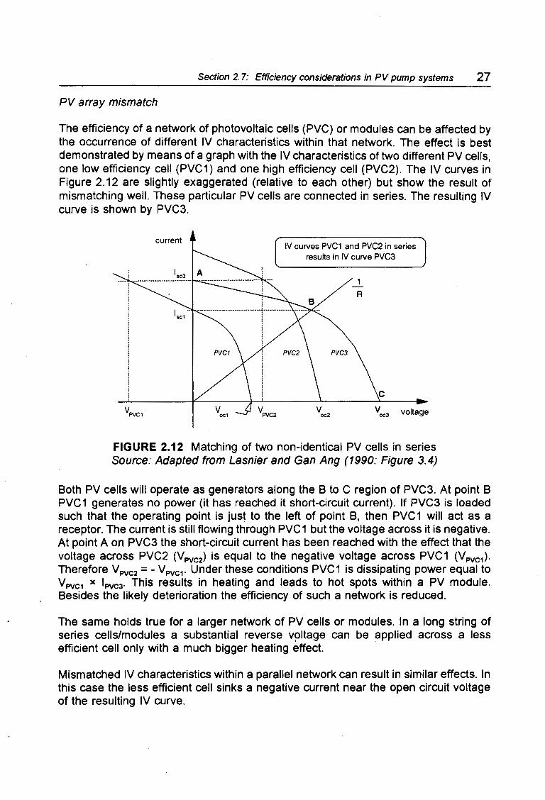
Univers
ity of
Cap
e Tow
n
Section 2. 7: Efficiency considerations in PV pump systems 27
PV array mismatch
The efficiency of a network of photovoltaic cells (PVC) or modules can be affected by the occurrence of different IV characteristics within that network. The effect is best demonstrated by means of a graph with the IV characteristics of two different PV cells, one low efficiency cell (PVC1) and one high efficiency cell (PVC2). The IV curves in Figure 2.12 are slightly exaggerated (relative to each other) but show the result of mismatching well. These particular PV cells are connected in series. The resulting IV curve is shown by PVC3.
current IV curves PVC1 and PVC2 in series
results in IV curve PVC3
PVC3
1
R
V oc3 voltage
FIGURE 2.12 Matching of two non-identical PV cells in series Source: Adapted from Lasnier and Gan Ang (1990: Figure 3.4)
Both PV cells will operate as generators along the B to C region of PVC3. At point B PVC1 generates no power (it has reached it short-circuit current). If PVC3 is loaded such that the operating point is just to the left of point B, then PVC 1 will act as a receptor. The current is still flowing through PVC 1 but the voltage across it is negative. At point A on PVC3 the short-circuit current has been reached with the effect that the voltage across PVC2 (Vpvc2) is equal to the negative voltage across PVC1 (Vpvc1).
Therefore VPVc2 = -Vpvc1• Under these conditions PVC1 is dissipating power equal to Vpvc1 x IPVcJ· This results in heating and leads to hot spots within a PV module. Besides the likely deterioration the efficiency of such a network is reduced.
The same holds true for a larger network of PV cells or modules. In a long string of series cells/modules a substantial reverse voltage can be applied across a less efficient cell only with a much bigger heating effect.
Mismatched IV characteristics within a parallel network can result in similar effects. In this case the less efficient cell sinks a negative current near the open circuit voltage of the resulting IV curve.

Univers
ity of
Cap
e Tow
n
28 Chapter Two: Photovoltaic water pumping
By-pass diodes are used to avoid the above phenomena. These diodes also protect strings of PV cells which may be partially shaded.
In an array where few strings of series modules are connected in parallel, the weakest modules can be separated into one series string and then connected in parallel to the other strings. This ensures that only one string of modules will generate a lower current. If the weak modules were distributed amongst the different series strings of modules then the overall array performance will be poorer. The rule is that the performancE3 of each string will be governed by the performance of its weakest module.
PV cell temperature variations
An increasei in the cell temperature results in a marginal increase in the operating current which is due to a decrease in the band-gap energy. However, the operating voltage decreases by a larger percentage than the percentage increase experienced by the operating current. The voltage decrease is due to an increase in the saturation current which is inversely proportional to the open-circuit voltage.
The overall effect of cell temperature on the maximum available array power is that the power decreases by approximately 0.35%/°C (Lasnier & Gan Ang 1990) as the temperatun~ increases (this figure will vary for different types of modules). Consequently the array efficiency is reduced by an increase in cell temperature.
Switch-mode controller
The efficiency of a controller is determined by three quantities namely the power requirements of the control electronics (analog or digitally based) and the drive circuit, by the switching losses and by the conduction losses.
Controller power requirements
The power requirements of the control electronics and the drive circuit are usually constant and include the efficiency of the power supply itself. The efficiency of a switch-mocle power supply is higher than the efficiency of a linear regulator-type power supply. The reduction in power requirements of the control and drive circuit electronics is a question of design and choice of components. The use of components that have a low powE~r consumption (for example, CMOS IC's) and an overall reduction in the number of components (for example, single chip computers with on-board ADC and phase comparator) will reduce the power requirements and can hence improve the efficiency. The improvements will be marginal as this area of control electronics and power electronics has been optimised to a large extent.

Univers
ity of
Cap
e Tow
n
Section 2. 7: Efficiency considerations in PV pump systems 29
Conduction losses
The conduction loss refers to the voltage drop which occurs across the switching transistor during periods of conduction (transistor on-state). A small, additional loss is incurred by the power dissipated in the diode across the other transistor (of one particular phase; refer to Figure 2.2).
The magnitude of the voltage drop is dependent on the on-state resistance of the transistor, on the peak line current (squared) which passes through it and on the power factor.
Conduction losses are reduced in power modules which have lower on-state resistance values. This is mainly a question of the available selection of power modules and their cost. It is also common to find converters (and. possibly inverters) which use a number of transistors in parallel to reduce the on-state resistance.
Switching losses
The switching losses which occur in the power module (MOSFET or IGBT) during the switching instances are directly proportional to the switching frequency of the controller. The major losses occur during the switch turn-on period whereas the turnoff losses are small in comparison. Turn-off losses are therefore regarded as negligible. The energy lost during turn-on depends on the shape of the line current waveform. The essential parameters are the peak current amplitude (the current overshoots on turn-on), the time base of the signal (from which the charge can be calculated: current x time) and the array voltage. The per phase dissipated switching power is therefore:
P switching = f. x V arr x iune (f" (time)) [W/phase]
The term i,;ne (f" (time)) represents the charge which is dissipated during turn-on. It is equivalent to the area under the switching current waveform during the switching instance. The total dissipated tosses are equal to three times P switching in the above equation.
The switching tosses are constant if the torque requirements and the. switching frequency are constant. A progressive cavity pump requires a reasonably constant torque and the variations in the line current are hence small. It is generally assumed that the switching tosses are constant under these conditions. They can however be treated as variable losses for a more accurate evaluation by taking account of the variations in the line current.
The switching tosses can be reduced by using transistors that have superior switching characteristics (shorter switch-on time) or by decreasing the switching frequency. However, a decrease in the switching frequency affects motor performance negatively.

Univers
ity of
Cap
e Tow
n
30 Chapter Two: Photovoltaic water pumping
Induction nwtor
The efficiency of an induction motor is affected by its design, by the harmonics in its current waveform and by the voltage to hertz relation applied to the motor. Considerations in terms of optimal motor design are not discussed as this goes beyond the scope of the dissertation.
Losses in the presence of harmonics
The harmonics in the voltage and current waveform do not contribute towards the real power transfer to the rotor shaft. This is done solely by the fundamental frequency components. The amplitudes of the harmonic currents generated in the motor inductance are independent of the load. They will be just as large at no-load as at full load (Schole!y 1982).
The harmonics in the current waveform result in losses which are primarily due to 12R
(copper) losses. Additional losses are due to core and stray losses as well as harmonic fre!quency eddy currents and hysteresis. These depend on the design and the material used in the motor. The latter losses are estimated to be in the range of 10% to 20% of the total power losses at rated load (Mohan 1989: 328).
Motor efficiency is improved when the harmonics in the motor current are shifted to high frequencies. This is accomplished by increasing the switching frequency.
Voltage to t1ertz relation
According to Davies (1992) the voltage applied to the motor has to be proportional to the square-root of the frequency to obtain an optimum efficiency over the whole variable frequency range. Davies also performed a sensitivity analysis which evaluated the reduction in efficiency due to variations in the required torque and the applied voltage. Both analyses showed that the reduction in efficiency is most marked at lower operating frequency. At 20Hz, torque variations of 20% result in a relative motor efficiency retduction of 2.3% (Davies 1992: Figure 31) and voltage variations of 20% result in a relative efficiency reduction of 5.6% (Davies 1992: Figure 32). At 70Hz, similar torque variations result in a relative efficiency reduction of 1.2% (Davies 1992: Figure 31) and similar voltage variations result in a relative efficiency reduction of 3. 7% (DaviE~s 1992: Figure 32).
The use of a progressive cavity pump will certainly result in some torque variations and depending on the magnitude of these variations, motor efficiency reductions as discussed aibove can be expected. If the load characteristics of a pump are very well known and are found to vary by relatively small percentages, then it would be possible to adapt the! voltage to hertz relation such that it would meet the torque requirements with minimal losses. The drawback is that the pump speed and inverter frequency have to be correlated to each other - pulley changes would therefore not be desirable once the ve>ltage to hertz relation had been optimised for a particular pump using a pre-determined speed ratio.

Univers
ity of
Cap
e Tow
n
Section 2. 7: Efficiency considerations in PV pump systems 31
Realistically this degree of voltage to hertz adaption is not possible as the required data would not be readily available. Furthermore, it is unlikely that the load characteristics of a pump (especially a progressive cavity pump) would retain its magnitude and shape over a longer period of time making a highly adapted V/Hz relation unwarranted.
Progressive cavity pump
The efficiency of the pump cannot be affected by changes in the installation but only through appropriate changes during its design stage. If a selection of pumps were available, then the most suitable pump for a particular site could be selected. This information is based on a paper by Vetter and Wirth (1992).
The losses which occur in a progressive cavity pump are mainly due to two factors:
(a) Losses due to slip - not all the water in the cavities is effectively lifted to the top, and a small amount of water slips back to the suction side of the pump;
(b) Losses due to friction between the stator and the rotor.
A typical efficiency curve is shown in Figure 6.19. The main variables are the pump speed, the pressure head and the interference fit between the stator and the rotor.
Losses as a function of pump speed
The friction losses tend to increase slightly as the speed of the pump increases (Vetter & Wirth 1992: Figure 6). The slip losses are usually close to 100% near zero speed and then decrease rapidly. For the particular type of pump mentioned in the paper (NE 20 Mono pump) the overall efficiency increases from about zero percent at zero speed to reach a peak at a third of its nominal speed and then decreases slightly for the remaining operating range.
Losses as a function of pressure head
The friction losses decrease substantially as the pressure head increases (Vetter & Wirth 1992: Figure 7) especially at low pressure head. Slip losses show a marginal increase as the pressure head increases. The overall efficiency of the pump increases from zero percent at zero head to its optimum efficiency at maximum and rated pressure head.
Losses as a function of the interference fit
The friction losses are virtually proportional to the interference fit. As the interference fit is narrowed (the stator is squeezed more tightly around the rotor) the friction losses increase (Vetter & Wirth 1992: Figure 8). The slip losses decrease rapidly as the interference fit is narrowed. The losses reach a shallow minimum from which they only increase slightly as the stator is fitted tighter to the rotor.

Univers
ity of
Cap
e Tow
n
32 Chapter Two: Photovoltaic water pumping
2.7.2 The impact of component interaction on the overall efficiency
The interaction of components can be divided into two categories namely, the mismatch losses and the transfer losses between the components. The losses are listed in Tab!e 2.4. The minimisation of some of these losses can improve the overall performance! of a PVP system.
TABLE 2.4 Areas of optimisation in a photovoltaic pump
Inter-component Mismatch losses Transfer losses
Sun~ array • spectral response • particulates and haze in the
• angle of array surface to sun 1> atmosphere
Array~ controller • tuning2> • cable copper losses7J
• array operating point3>
• size of input capacitor(s)4>
Controller ~ motor • none other than the V/Hz • cable copper losses7J relation and current harmonics as discussed in subsection 2.7.1
Motor~ pump • unreasonable speed ratioSJ • friction in belt transmission
• pulley misalignment6J
Pump ~ rese1rvoir • too small pipe diameter • discharge head gland packaging8>
• sudden pipe expansion • friction in discharge head
• sudden pipe contraction bearings9>
• friction and velocity head losses in pipe network - roughness
1> If the angle (a.) between the direct component of the global irradiance and the
normal to the array surface is larger than zero degrees the amount of direct irradiance received is reduced by (1 - cos a.) x 100 [%]percent. The amount of incidemt irradiation during the course of a day/year can be maximised by the use of different array structures. The options are a fixed array with no seasonal adjustment (worst case), a fixed array with seasonal adjustment, a single axis tracking array and a dual axis tracking array (best case).
2> The most common operating modes implemented by PVP controllers are: fixed
voltage operation (FVO), optimum voltage point tracking (OVPT) or maximum power point tracking (MPPT). FVO and OVPT require tuning. The specifications for the modules are required for that. In case of FVO the array voltage should be chosen closest to optimum array operating point by taking account of the most probable average cell temperature for the particular site.
3> Steady :state and instantaneous array operating point should be stable, that is no oscillations about an average point as this can diminish the array output power.

Univers
ity of
Cap
e Tow
n
Section 2. 7: Efficiency considerations in PV pump systems 33 -. ~·." . . . . ;
4> The size of the input capacitor has an effect on the magnitude of the ripple
current at the controller input and it affects the capacity to provide the required starting torque. Over-sizing the capacitors is mainly prohibited by cost. An increase in capacitance requires a reassessment of the start-up amplitude programmed into look-up tables since the higher current generation capabilities of the increased capacitance can damage the power module on start-up should it exceed the controller power module ratings.
5> The two extremes are: a) a too large speed ratio (small motor pulley) where
the motor will reach maximum speed at low input powers and b) a too small speed ratio (large pulley ratio) resulting in torque requirements that cannot be met by the motor (in conjunction with the array current and the DC capacitors).
6> Pulley misalignment will result in unnecessary friction in the transmission. The
motor pulley can be adjusted until the V-belt plane is at right angle to the motor and discharge head plane where latter planes face each other.
1> The voltage-drops over long cables can be reduced by using larger diameter cable; the trade:.off is higher cost - an assessment has to be made from case to case.
8> Gland packaging material which has less friction than graphite asbestos but also acts as a good seal will reduce losses; Payne (1986) suggests replacing graphite asbestos with P.T.F.E. (a form of teflon).
9> These bearings could be replaced with non-contact type sealed bearings (Payne 1986).
/

Univers
ity of
Cap
e Tow
n
36 Chapter Three: System description
3.2 The array
The PV arra~r consisted of twelve monocrystalline modules manufactured by Siemens. However these modules were not all from the same production generation. The breakdown was as follows:
3 x M55 4 x M55S
5 x IVl55
ARCO Solar modules (black aluminium frame) Siemens Solar modules (silver aluminium frame, with M6 nuts pressed into the frame to simplify installation) Siemens Solar modules (silver frame, youngest generation)
The specifications and the physical dimensions remained the same for all three types of modules except for a small increase in the short circuit current in the most recent gener.ation of modules. Temperature coefficients were only supplied for the M55S while the specifications of the other two module types included graphs showing the effect of temperature on the array voltage.
3.2.1 Spe1cifications
The data sheet for the Siemens module is attached in appendix A 1.1. The Table below lists the specifications of the M55S module. Each module was fitted with two by-pass diodes.
TABLE 3.2 Specifications of a Siemens M55S module
Output'' Value Units
MPP voltage 17.4 VMPP
MPP current 3.05 AMPP
Open circuit voltage 21.7 voe Short circuit current 3.35 ~ Maximum power 53.0 WP Efficiency 13.9 %
Temperature performance
NOCT 21 47 oc Temperature coefficient of V ~ tv - 0.34 %1°C Temperature coefficient of la; t, + 0.04 ·%1°C
Module Area
Number of cells per module 36 Cell area 0.0106 m2
Module area 0.3812 m2
1> These electrical characteristics can vary by :t:10% due to manufacturing variations. Standard Test Conditions (STC) are: irradiance of 1000W/m2, cell temperature of 25°C and air mass of 1.5.
2l NOCT: Normal operating cell temperature: lrradiance = 800W/m2, ambient . temperature = 20°C and wind speed 1 mis.

Univers
ity of
Cap
e Tow
n
Section 3.2: The array 37
3.2.2 Configurations used
The three electronic controllers under test had different voltage limits on their input. The array therefore had two configurations: one series configuration where all the modules were in series, and one parallel configuration where two strings of six series modules were connected in parallel. The expected output values of the array for both configurations are listed in Table 3.3.
TABLE 3.3 Possible array output values for series and parallel configuration
Output: Series configuration 1> STC NOCP> Units
MPP voltage 208.8 193.23) VMPP
MPP current 3.05 3.083) AMPP
Open circuit voltage 260.4 240.9 voe Short circuit current 3.35 3.38 Ase
Maximum power 636 595 WP
Output: Parallel configuration 1>
MPP voltage 104.4 96.63) VMPP
MPP current 6.10 6.163) AMPP
Open circuit voltage 130.2 120.5 voe Short circuit current 6.70 6.76 ~ Maximum power 636 595 WP
A"ayarea
Total array cell area 4.5742 m2
1> These values are given as an indication only. Inter-module mismatch and transfer losses have not been taken into account.
2l NOCT = 4 7°C and G = 800W/m2 but here it is calculated for 1 OOOW/m2 as this is more representative of Namibian solar irradiance conditions.
3> These values assume that the open-circuit voltage and the short-circuit current
temperature coefficients are the same for the MPP voltage and current.
3.2.3 Tracking array mechanism
The array was a single-axis, passive tracker with two tilt angles to accommodate seasonal changes. It was manufactured by Zomeworks in the USA. The data sheet is in appendix A 1.2. The tracking principle is as follows: The array has a black metal tube on the east and the west side that contains a gas (CFC). Both tubes are connected with a compensating pipe. Both are partly shaded with U-shaped aluminium wings (see appendix A 1.2) that partially cover the top surface and the bottom surface of the tube, leaving a section exposed to the sun for heating. These sections are heated in equal amounts when the sun shines perpendicularly on the array. Tracking is accomplished when the sun is not shining perpendicularly onto the array since, under these circumstances, one tube is heated more than the other and the gas then expands and forces most of its weight into the less heated tube. The imbalance in weight causes the array to turn while shock-absorbers prevent fast movement.

Univers
ity of
Cap
e Tow
n :c :::.
CJ)
!! 3: 0
u:::
38 Chapter Three: System description
3.3 The pump
3.3.1 Specifications
The pump that was used was a S2M Mono borehole pump. This is a positive displacement, progressive cavity, self-compensating stator type pump. It operates up to a head of 150m. The maximum recommended speed is 1200 rpm. Th.e specified minimum starting torque is 3N.m.
The pump data sheet is in appendix A 1.3. Figure 3.1 a shows the pump characteristics at 75m in a slightly reprocessed form.
1400
1200
1000
800
600
400
60
·····-············--········-·-· 50 flowrate "#.
i··-·····-··········-·-····-·-·--···-.,;.--··-··---·-··-··-··,t;---·····-·-···········-----·········-·······-·- 40 >-(,J c
i··-·--···---····--r····-·--···-·--····----··-J&···-···-·····-·······--·-···-··-·-·····-··--············-·-······ 30 -~
+--·--·•·------QI····----·--···-·-----···-----·-- 20 ffi
200 ·--·---·7··---·······-·--·····-·-········-( Static head = 75m J 1 O
0 0 0 100 200 300 400 500
Pump input power [W]
(a)
'E 2.s --·---in ~ ' ~ 2.0 ---·----··--------· -··-_Q
o.op.::::;;,--~-----.------..-----1 0 400 800 1200 1600
Flowrate [l/h]
(b)
FIGURE 3.1 Supplied data for S2M pump: (a) Flowrate and efficiency of the pump at 75m; (b) Rising main head losses
3.3.2 Installation
The pump was installed at a depth of 90m. The pipe had a diameter of 40mm. The shaft had a diameter of 13mm and was supported by bobbin bearings (one per 1.5m). A graph that shows the head losses as a function of the flowrate in the rising main pipe was supplied by Mono Pumps. The relevant section of the graph (in terms of flowrate) is shown in Figure 3.1 b.
3.3.3 Transmission
The power of the motor was transferred to the pump by means of a single V-belt (Super-HC; 1oxamm). The section type was 10N (SPZ) which was the narrowest section ava1ilable. The pulley on the discharge head assembly had an outer diameter of 250mm. The pitch-centre diameter (PCD) was measured to be 247mm. The motor pulleys that were available for the tests were: 85, 97, 112, 118, 125 and 140 PCD.

Univers
ity of
Cap
e Tow
n
Section 3.4: The Mi"ek DC to DC converter 3 9
3.4 The Miltek DC to DC converter
3.4.1 Specifications
The Miltek converter as used in the tests was a DC to DC converter, model number MEI 400. It was manufactured by Miltek Electrical Industries which has become a subsidiary of United Power Corporation. In the text the converter is referred to as Miltek converter.
TABLE 3.4 Specifications of the Miltek converter
Input Value Units
Operating range for fixed vo"age 1J 45 ~ 120 varr
Maximum open-circuit vo"age2J 200 varr
Maximum short-circuit cu"ent 15 Aarr
Output
Voltage range3J (0.06 ~ 1) >< <Varr - 1.4) v
Maximum pulsed cu"ent Maximum power Switching frequency Efficiency (direct mode)
Other
DC Capacitance (200V) External fuse
Mode of operation
25 A 1.6 kW 2.5 kHz 96 %
2200 µF 10 A
Fixed Voltage Operation (with direct mode)
1> This voltage is fixed during converter operation (except in direct mode). For operation
near the maximum power point, this voltage can be fixed to roughly n><VMPP where n is the number of modules in series. Usually n ~ 3 and ~ 6. During direct mode the voltage can exceed 120V as the operating point could move down the IV curve.
2l This limit is set by the maximum voltage across the capacitors and possibly by the power supply. In terms of modules this means eight(>< 25VoJ for 200V maximum.
3> The minimum output voltage is a function of the array operating voltage and the duty ratio of the narrowest pulse that the PWM unit can generate. The maximum output voltage is a function of the input voltage, the converter current, R
0" and the load. If the load is well matched then the converter will go into direct mode
at full irradiance. At that point the output voltage is close to the input voltage minus the voltage drop across the MOSFET's. At Ron = 0.1 n and drain current of 14A the voltage drop is 1.4V. This is very small but can be higher if Ron increases with temperature.
3.4.2 Configuration of the converter in the PVP test system
The PV array was connected in parallel configuration. Therefore the input voltage was fixed to approximately 92V.

Univers
ity of
Cap
e Tow
n
40 Chapter Three: System description
' 3.4.3 Co1r1trol algorithm
The converter electronics is implemented purely with analog circuitry. For this reason there is no software. The control algorithm is part of the hardware.
The array voltage is the control variable. If the array voltage is less than the reference voltage then the voltage applied to the motor (converter voltage) is decreased. This results in a decrease in motor speed (motor voltage oc motor speed). If the array voltage is larger than the reference voltage then the motor voltage is increased. The aim is to have a fixed array voltage and the motor is driven in such a way that this can be impleme1nted.
The converter operation at start-up is linear which means that it does not employ any special routines to overcome the break-away torque of a positive displacement pump (the energy could be generated out of the DC capacitors). The converter is however capable to connect the array directly to the motor (MOSFET in a continuous on-state) once the converter receives sufficient current from the array to supply the pump torque requirements. When the converter enters the direct mode it leaves its fixed voltage operating point and moves towards a higher voltage operating point. This takes place whenever the irradiance increases beyond the threshold value (where the array current meets the required motor current).
3.4.4 Har·dware
Figure 3.2 shows a basic block-diagram of the Miltek converter (linear current booster) in the PVP system. Some more detail is given below.
Array
Miltek Power Supply
I Miltek power stag~
array PWM voltage
Miltek controller
Adjustments
reference voltage
switching frequency current limit
control loop dead time
FIGURE 3.2 Basic block-diagram of the Miltek converter

Univers
ity of
Cap
e Tow
n
Section 3. 4: The Miltek DC to DC converter 41
Control and drive circuitry
The converter voltage is varied by pulsing the array voltage. This is achieved with the MOSFET's at a switching frequency of 2.SkHz (factory set). By changing the pulsewidth the converter voltage can be increased or decreased. The duty ratio is directly proportional to the output voltage. The PWM signal is provided by the control circuit (implemented with PWM IC SG3524) to drive the MOSFET gates.
Due to superior performance of N-channel over P-channel MOSFET's, N-channel MOSFET's are used to switch the negative DC bus (see Figure 3.2). Therefore the positive array voltage terminal and the positive motor terminal are permanently connected.
Power device
The converter uses three IRF350 MOSFET's in parallel. The ratings of a single MOSFET are as follows:
• maximum drain-source voltage is 400V • continuous drain current is 14A • pulsed drain current is 25A • on-state resistance is approximately 0.30 • maximum power dissipation is 1 SOW
As the three MOSFET's are connected in parallel the on-state resistance (0.30) is reduced to 0.1 o. This results in lower losses.
A free-wheeling, fast-recovery diode facilitates smooth operation by providing a path for the motor current when the MOSFET's are switched off.
Power supply
This would appear to be a linear voltage regulator. A 25W, 1.SkO resistor reduces the array voltage which is fed into a transistor with a Zener clamp at its base. The output is then regulated to the required voltage.
Adjustments
Four potentiometers are provided for adjustments. Only P1 would ideally require tuning. The other three potentiometers are factory-set.
P1: A multi-turn pot to adjust the array reference voltage (FVO). It is usually set to 0.76 x voe but might require adjustment at the installation site. For various array configurations the fixed voltage can be adjusted over a range of 45 to 1 SOV.
P2: A single-turn pot to adjust the switching frequency. It is set to 2.SkHz.

Univers
ity of
Cap
e Tow
n
42 Chapter Three: System description
P3: A single-turn pot to adjust the current limit which is factory-set to 15A.
P4: A single-turn pot to adjust the control loop dead time
3.4.5 Signal profile
The graph below shows the characteristic curves of a DC to DC converter .. The converter current ramps up during the on-cycle of the converter voltage and down during the off-cycle. The converter output voltage (pulse height = array operating voltage) is controlled by controlling the width of the pulses (PWM). The fact that the current can flow during the voltage off-cycle is due to the free-wheeling diode.
100-.--------'~-------------.-24
voltage ...----""" 75 --------··- -···-··---·-··----·····-·· --·-·- -p-N"-/ __ +------1-----4-21
50 ---·~---··---··--- -----·· --1------+18
25 ---- -····--··-··-- ·-··---1------t-- t----+15 -~
~ o~-------....... -------------..i----...... --r12 ~ ~ ~ 0 ~ > 9 (.)
-50
-75 current
-100;-------..----.------.--""'--....-----+0 0.0 0.2 0.4 0.6 0.8 1.0
Time [msec]
FIGURE 3.3 Characteristic converter output signals
The magnitude of the current is dependent on the load. If the load increases then the current will ramp up to a higher peak value during the on-cycle. There is no phase angle between these two signals which is to be expected from a DC system.

Univers
ity of
Cap
e Tow
n
Section 3.5: The Salvo three phase inverter_ 43
3.5 The Solvo three phase inverter
This three phase inverter was designed and developed by Gunther Hirschmann in Germany. The inverter, being still in the prototype phase, does not have a model name/number. Salvo refers to the name of Mr Hirschmann's company and the inverter is referred to as the Salvo inverter.
3.5.1 Specifications
TABLE 3.5 Salvo inverter specifications
Input Value Units
Voltage operating range 120--+ 190 varr Maximum open-circuit voltage 1
J 270 varr Maximum short-circuit current (B0°C) IGBT: 15, FET: 13 Aarr
Output MOSFET BSM 652 F -or-IGBT BSM 15 GD 1000
Line to line voltage (as programmed) (0.184--+ 0.612) x varr V rrns
Maximum pulsed current at 80 °C IGBT: 30, FET: 52 A Maximum power 1.8 kVA Frequency range (as programmed) 7.6--+ 84.7 Hz Switching frequency (as programmed) 10.3 --+ 17.5 kHz Efficiency (estimated) - 90 %
Other
DC input capacitance (350V) 1100 µF DC side fuse 4 A Array voltage readings in intervals of: 10 ms Max. temperature of power module 80 oc
Mode of operation Fixed Voltage Operation
1> This limit is set by the power supply maximum input voltage
3.5.2 Configuration of the inverter in the PVP test system
The PV array is connected in series configuration for this inverter. The input voltage is fixed approximately to 185V. The maximum line-to-line rms voltage is therefore 113V.

Univers
ity of
Cap
e Tow
n
44 Chapter Three: System description
3.5.3 Hardware
The inverter consists of two printed circuit boards (PCB). The large PCB holds the DC capacitors, tlhe gate drive circuitry and the power supply. The smaller PCB holds the microcomputer which consists of a microcontroller with its peripheral components. The power module is mounted on the inverter cast-aluminium casing for heat transfer. Both PC B's are fully visible from the top. A single-turn potentiometer for tuning the set-point of the array voltage is mounted on the microcomputer board and can be adjusted from the top (it has been moved to the drive circuit PCB in the more recent prototypes).
Figure 3.4 shows a basic block-diagram of the Solvo inverter. A detailed description follows below.
Array
demodulator Solvo Driver HF transformers
and Power modulator
Stage Adjustments
v reference voltage may
pulsed current limit
controller temperature threshold
FIGURE 3.4 Basic block-diagram of the Solvo inverter
Microcomputer
The microcomputer consists of the SAB 8031 microcontroller, a dedicated PWM generation IC (SLE 4520), an 8-channel analog-to-digital converter (ADC 0808) that digitises the reference array voltage and a 4kbyte EPROM (2732A) containing the program codle. In addition, there is a frequency divider (74LS161), a bus-driver (7 4HC673) and an IC with six open collector transistors (7 406).
The salient features of the SAB 8031 are volatile 128 >< 8bit RAM, four programmable 8-bit 1/0 ports, two 16-bit programmable timer/counters, two external and three internal interrupt lines (2 timer and one serial interrupts) with two priority levels, a serial 1/0 line, an on-chip oscillator and clock circuits. The timers are essential as they can be used (and an:!) to process the PWM pulses at regular intervals. The controller runs at a clock frequency of 12MHz. This is the recommended clock speed for the 8031 processor and the SLE 4520 PWM IC combination.

Univers
ity of
Cap
e Tow
n
Section 3. 5: The Solvo three phase inverter 4 5
The main features of the SLE 4520 are its capability to generate motor frequencies from zero to 3 kHz at switching frequencies of up to 23.4 kHz, to generate an almost unlimited range of waveforms with any phase relationship (smallest increment of 7 .5°) and to adapt to different power stages due to a programmable dead time (dead time is essential to avoid bus shoot-through in case the upper and lower device have unintentional switch-on overlap periods). Changing the switching frequency in steps of one microsecond results in a virtually continuous transition from one motor frequency to another.
The SLE 4520 consists of the following functional blocks:
• A crystal oscillator input (a 12MHz crystal is used). The oscillator provides a buffered clock output that is used by the microcontroller.
• Two 4-bit registers for dead time and a divider ratio. The latter sets the clock frequency at which the SLE operates (2MHz). These registers only need to be written once, usually in the initialisation phase of the microcontroller.
• Three 8-bit phase registers which are continuously being written. The values that are received are latched into down-counters on reception of the transfer pulse (SYNC) from the 8031. The zero detector will be low (as the content of the downcounter is still non-zero) which will enable the counters. Therefore the pulse starts and ends when the zero detector goes high. The next pulse is sent when receiving the next transfer pulse.
• An output block, which receives the signals from the phase registers and generates their inverse (to drive six switching devices) and adds the programmed dead time to the pulses. The unit also blocks the output (all signals go high, that is the active switching state is Low) when receiving a High on the Inhibit or the Status line.
• An address decoder that decodes a three bit address from the 8031 to enable one of the five registers to receive data.
The 7 406 IC with the open collector transistors has the following functions: Raising the PWM signal voltage to 12V, inverting the PWM signal (the SLE switches active low) and buffering the output of the SLE.
Protection from overheating is provided through a heat sensitive resistor which is mounted on the power module. At a tunable threshold level, a comparator switches to a low logic state activating an interrupt. This results in a state of in-operation until the power module has cooled down sufficiently.

Univers
ity of
Cap
e Tow
n
46 Chapter Three: System description
Short circuit protection on the AC side is sensed on the DC side with a torroid-type transformer by measuring the current surge that occurs during a short-circuit. If the current exceeds a particular, adjustable threshold then a flip flop at the SLE 4520 is pulled high which will inhibit any further output. This circuit has a very fast response since it disables the SLE directly.
The inverter is overload protected by a three phase thermal switch. The data sheet for the AEG Mbs 25 protective motor switch is in appendix A 1.4.1.
Drive circuit
The most central aspect of the drive circuitry is the provision of an isolated signal to the gates of the power switching devices (Hirschmann 1989a). This gate drive circuitry structure is based on high frequency (HF) transformers rather than opto-couplers. The reason for this choice is that at the time the inverter was developed the available range of opto-couplers did not fulfil the requirements (to be fast and to have a small coupling capacitance).
Besides the advantage of complete isolation between the driver stage and the power module, the gate voltage for the three upper FET's is derived via the HF transformers (see Figure 3.4).
HF transformers are usually sized for a particular frequency. Their design becomes non-trivial if the transformer has to transfer pulses of variable duty cycle (like a PWM signal). The PWM signal is therefore modulated with a frequency higher than the frequency of its narrowest pulse. The narrowest pulse here is 1 µs (1 MHz) and the carrier frequency is 3MHz.
The PWM signal and its inverse is modulated with the 3MHz carrier signal (obtained from the 12MHz clock frequency divided by four) by means of an AND and a NANO gate. The resulting signal is amplified with two push-pull stages and then coupled across the HF transformer. On the secondary side, the PWM signal is restored through the removal of the carrier signal by means of fast rectifier diodes leaving the envelope curve with a superimposed ripple. The 3MHz ripple on the PWM signal is smoothed by the high watt resistor in conjunction with the Gate-Source or Gate-Collector input capacitance of the MOSFET or the IGBT power module. Some additional capacitance (2.2nF or 4.7nF respectively) has been added to further reduce the magnitude of this ripple. The ripple has to be kept below a certain level to avoid ringing after switch-off. A 16V Zener diode limits the voltage spikes that occur when the MOSFET's or the IGBT's are switched on. A PNP transistor decreases the switch-off transition time.

Univers
ity of
Cap
e Tow
n
Section 3. 5: The So/vo three phase inverter 4 7
MOSFET power module BSM 652 F
The three phase full-bridge SIMOPAC power module from Siemens consists of six MOSFET's in a single package. Each MOSFET is equipped with a Fast Recovery Epitaxial Diode which make these FET's particularly well suited to switch inductive loads. The MOSFET's are of the N-channel type. Some characteristics of the module are: drain-source voltage of 500V, continuous drain current of 13A (at 80°C), pulsed drain current of 52A (at 80°C), Roscon> of 0.28 to 0.32Q (for V05 = 10V), a turn-on time of 150ns and a turn-off time of 420ns.
IGBT power module BSM 15 GD JOOD
The IGBT (Insulated Gate Bipolar Transistors) power module has become the replacement for the MOSFET module. It also contains six transistors and has the same physical dimensions as the MOSFET power module. The advantage is that the IGBT is more robust. It has a maximum collector-emitter voltage of 1 OOOV, a continuous collector current of 15A (at 80°C) and a pulsed collector current of 30A (at 80°C). The on-resistance, Ree• is typically 0.15n, compared to 0.30Q for the MOSFET. One disadvantage is the switching characteristics which are slightly slower than those of the MOSFET's (turn-on time = 250 ns and turn-off time = 450ns). A data sheet is attached in appendix A 1.4.2.
Power supply
A switched-mode power supply has been implemented in this inverter. The input voltage can have any value between 60 to 270Voc. It basically consists of a control IC, a MOSFET and a transformer which consists of two sets of primary and secondary coils. The main primary coil couples the demanded power across and the other primary coil works as a feedback of the power demand on the secondary side. The secondary side coils provide two different voltages (5 and 15V). The control IC used is the TOA 4605. It 'observes' whether the voltage is constant, dropping or increasing and responds by switching the MOSFET accordingly. As a result the secondary side voltages remain almost constant. Rectification takes place on the secondary side of the transformer
3.5.4 Software
Program features
The inverter drives the motor through a maximum of 16 major gears if enough power is available (Gear Oto Gear 15). Each major gear has 16 minor gears resulting in a maximum of 256 gears for the full frequency range. The present programs only utilise 11 major gears (Gear 5 to Gear 15) resulting in a resolution of 176 gears for the 85Hz frequency range. The inverter starts a run-up through Gear O to Gear 4 with an amplitude modulation index of zero. Therefore the resulting line-to-line voltage is zero. The inverter then starts the motor in Gear 5 with a frequency of 7 .6Hz. The change in frequency within one major gear is not constant however (for example, if we say

Univers
ity of
Cap
e Tow
n
48 Chapter Three: System description
that the full frequency range is equal to 80Hz and the number of major gears is equal to 1 O; then 80/1 O gears is equal to 8Hz frequency-change per major gear which is not true). Typically the change in frequency in the lowest major gear is about 2Hz (Gear 5) and in the highest major gear about 13Hz (Gear 15). Therefore the frequencychanges within a minor gear at low major gears are about 0.12Hz (2/16) and increase to about 0.81-lz (13/16) at high major gears.
The Volts to Hertz relation can only be adapted to the frequency of the major gears and not the minor gears. Therefore the voltage increases are comparatively large (from about 30V to 11 OV in 11 steps). The shape of the V to Hz curve is stored as sine-weighted PWM values in look-up tables.
PWM generation
When switching at frequencies of up to 15kHz the number of different width pulses that would be required to generate a low frequency fundamental waveform is enormous (a 20 Hz signal would require 375 different width pulses). Such a signal cannot be generated with an 8-bit (= 128) word. Therefore pulses of equal width have to be repeated a fixed amount of times (anything between 1 to 255 times is possible). This repetition value is changed between major gears but remains the same within a major gear. The repetition rate for equal pulses is greater at lower fundamental frequency than at higher fundamental frequency, assuming that the switching frequency stays more or less constant throughout the range of major gears.
The above-mentioned point explains more clearly how the inverter manages to change its fundamental frequency between major gears. A decrease in fundamental frequency is achieved through increasing the number of times that each different pulse is repeated (the effect is almost as if the waveform is being stretched). The opposite is true for an increase in fundamental frequency. The 'jump' in frequency from one gear to another can be minimised by slightly adjusting the switching frequency.
Frequency changes within a minor gear are effected by changing the time-base for the timer interrupt. This is done in steps of 1 µs. To clarify matters further, the Timer O of the 8031 is responsible for sending the three PWM values from the look-up table to the SLE 4520 phase registers. It is also responsible for sending the SYNC (transfer) pulse at regular intervals. These intervals are changed in steps of 1 µs for a small frequency change in minor gears. Therefore the switching frequency changes by 16µs within each major gear. For example, if the switching frequency is equal to 12.5kHz (80µs) in the first minor gear then it will be 15.6kHz (64µs) in the sixteenth gear. It is up to the programmer and hardware limitations whether or not the next major gear has the same switching frequency spectrum.
The 8031 and the SLE 4520 combination is not able to operate at modulation indexes which are larger than one. Therefore over-modulation is not possible and the voltage of the array at the maximum power point should be high enough to achieve the rated voltage of the motor (at a modulation index of one, the rms voltage is equal to 0.612 x array voltage (Mohan et al. 1989: 132)).

Univers
ity of
Cap
e Tow
n
Section 3. 5: The Salvo three phase inverter 4 9
Algorithm
The array voltage (from the ADC at intervals of 1 Oms) is the only variable used by the control algorithm to determine whether or not the motor frequency should be increased or decreased. As this inverter runs in FVO mode, the software reference value is fixed. The algorithm attempts to remain as close as possible to this value and will increase the motor frequency (ie, increase the load) when the array voltage is larger than the reference value, and decrease the motor frequency when the array voltage is lower.
The algorithm continuously tests the state of the phase reversal switch which can be activated during inverter operation. Should the switch be activated, the algorithm will stop the motor by running down through all the gears. The inverter will start up again after about 5 seconds the motor turning in the opposite direction.
Over-heating is constantly monitored. When it occurs, the motor is switched off and the microcontroller waits until the temperature has decreased to below a particular threshold.
3.5.5 Signal profile
Figure 3.5 shows some of the characteristics previously mentioned. Graph (a) displays the line-to-line PWM pulses. The vertical lines divide the pulses into groups of four which have the same width. This is not easily visible on the graphs but the data values show this clearly. From the number of repeated pulses and the switching frequency (if there were enough resolution) one could calculate exactly in what major and minor gear the inverter is.
300
250
Q) 200 ~ = g 150
Q)
.~ 100 6 d; 50 c
:.:J 0
-50
r-- same pulse width
p ! ~ v ~ I
I
--.. ~
I
~
20,--~~~~~~~---;:========il I Gate-drive signal I
~ Q) 10~--'------1---+------t ~ = ringing g Q) 5~--------t---N-----t
1ij (!)
0.4 0.6 0.8 1.0 1.2 1.4 1.6 1.8 2.0 ·5
4 6 8 10 12 14 16 18 20
Time [micro-sec) Time [msec]
(a) (b)
FIGURE 3.5 Some Salvo inverter characteristics
Graph (b) shows the ripple on the gate-drive signal which is the remains of the carrier frequency. A suitable gate-source capacitance has to be selected to reduce the ringing effect without increasing the switch-off time too much.

Univers
ity of
Cap
e Tow
n
50 Chapter Three: System description
Figure 3.6 shows a typical current and voltage signal sent out by the inverter in conjunction with a three phase motor.
~: Q) Cl (1)
.:!: 0 >
200~-----------....,..----------.-8
100
50
0
-50
-100
-150
-200
-·
·-"'
--
line-to-line ..................... . .. _,,, .. ___ ,,, .. , ___ ,,,,_, _____ ,_ 6 ~ voltage
line current
-0 ~ ''-:::i
-2 ()
-4
-6
+--...:.....-----.---.-----.-----.---r-=-----.----+-8 0 5 10 15 20 25 30 35 40
Time [msec]
FIGURE 3.6 Current and voltage of the Salvo inverter
3.5.6 Future developments
The new opto-couplers from Toshiba, the TLP 251 's, are fast enough to process the PWM signals at this high switching frequency range. They could therefore replace the AND and NA.ND gates, one of the amplifier stages and the HF transformers, thereby rendering thE~ modulation of the PWM signal unnecessary. This would result in fewer parts, reduce~d costs and higher efficiency, the latter due to reduced switching losses resulting from shorter rise and fall times (rise time = 200ns and fall time = 1 OOns). Improved reliability is debatable.
The microcointroller will be replaced with the SAS 80517 which is an 8-bit single-chip microcontroller. It has an on-board phase comparator which would simplify PWM generation when compared to generating the PWM from the 8031 directly. This implementation would result in reduction of parts on the microcomputer board and should increase the mean time between failures.

Univers
ity of
Cap
e Tow
n
Section 3. 6: The ML T three phase inverter 51
3.6 The ML T three phase inverter
3.6.1 Specifications
This three phase inverter was designed by John Davies in partial fulfilment of an MSc degree in Engineering at the University of Cape Town. It was developed to the prototype stage at ML T Power Electronics in Cape Town. It is referred to as an ML T inverter in this dissertation.
TABLE 3.6 Specifications of the ML T inverter
Input
Voffage operating range Maximum open-circuit voffage Maximum short-circuit current
Output
Line to line voffage (as programmed) Maximum continuous current at 60 °C Maximum power Frequency range Switching frequency range Efficiency over main operating range
I Other
DC Capacitance (200V) Array voffage readings in intervals 11
Speed reading intervals 11
Max. temperature of power MOSFETs
Modes of operation
Value Units
80 ~ 120 varr 200 varr
8 A arr
MOSFET IRFP 250
(0.184 ~ 0.73) x varr vrms 33 Arms
0.5 kVA 3 ~s5 Hz
o.8 ~s kHz - 85 %
2040 µF 80 ms
2000 ms 150 oc
Fixed voltage operation Maximum speed tracking
1> There is some uncertainty about these values. It is certain however that for every speed reading there were 25 array voltage readings
3.6.2 Configuration of the inverter in the PVP test system
The PV array was connected in parallel configuration for this inverter. The input voltage was adjusted to approximately 95V. The maximum line-to-line rms voltage was therefore 69.3 Vat an array voltage of 95V.
3.6.3 Hardware
The inverter consists of two PC B's. One PCB holds the microcomputer which consists of a microcontroller with its peripheral components. The other PCB holds the gate drive circuitry. The power switching devices are soldered onto the gate drive PCB with

Univers
ity of
Cap
e Tow
n
52 Chapter Three: System description
their backs mounted to a heat-sink which is attached to the inside of the inverter castaluminium casing. The power supply is also mounted on the heat sink. The DC capacitors are attached to the bottom of the drive circuit PCB by means of plastic straps. The microcomputer PCB is mounted above the gate drive circuit PCB. Two multi-turn potentiometers, of the front adjustment type, are mounted on the microcomputer PCB for tuning the array voltage and the motor speed references voltages. A basic block-diagram is displayed in Figure 3. 7 showing the functional blocks of the ML T inverter.
Array
Microcomputer
I Power i
L_Sra~.,~~--+--+~-+--+-_J array voltage
MLT controller
motor speed
Adjustments
reference voltage
reference speed
FIGURE 3.7 ML T inverter block-diagram
The main components on the microcomputer board are the Intel 8031 microcontroller, one 8-channel ADC (ADC 0809) that converts the voltage references for the array and the motor speed, one 8kbyte EPROM (27C64) containing the program code and one 2k RAM chip (6116). A frequency divider in the form of four D-type flip-flops divides the clock frequency by 16 for the ADC. A few NANO gates are used for chip enabling, read, write and status signals etc. A frequency-to-voltage converter (LM331 N) and an active LPF (CA7140) make up the speed reference circuit and an oscillator IC (LM555) forms part of the watchdog circuit.
The main features of the 8031 microcontroller were described earlier (subsection 3.5.3). The clock frequency provided to the 8031 is 10MHz. The controller is interfaced to ROM, RAM and the ADC. The PWM signals are latched from the 8031 through Port1 (P1 .0 to P1 .5) driving the opto-coupler LED's directly.
Speed monitoring is facilitated by means of a magnetic speed sensor. The LM331 is configured as a frequency-to-voltage converter. The signal is converted in the ADC and is read into the 8031 to act as a second level control variable.

Univers
ity of
Cap
e Tow
n
Section 3.6: The MLT three phase inverter 53
The speed sensor signal is also fed to the watchdog circuitry (implemented with the LM555). The circuit provides the logic to the 8031 indicating whether or not the motor is running. If the motor is at standstill, the 8031 is reset with a high on its RST pin of longer than two machine cycles and performs a restart. If the speed sensing option is not used then the watchdog circuit can be supplied with one of the PWM output signals from the microcomputer board.
Drive circuit
This circuit structure is based on opto-couplers. All six PWM signals from the 8031 are coupled via 4N32 opto-couplers. This protects the microcontroller from possible voltage surges due to power device switching. The coupled signals are fed into 050026 totem-pole drivers which are capable of supplying high current pulses and have, in addition, fast turn-on and turn-off times.
The circuit has a switching aid network to reduce turn-off time. It consists of an RCD snubber circuit made up of a resistor, a capacitor and a diode.
Power device
The power stage consists of six separate IRFP250 MOSFET's. These FET's are based on HEXFET technology which achieves very low on-state resistance (0.0850 at a drain current of 33A and a temperature of probably 25°C; the on-state resistance increases to 0.1060 at a temperature of 60°C). It has superior diode recovery dv/dt capabilities. The internal diode also acts as a Zener diode. Further characteristics include an N-channel type FET and a maximum drain-source voltage of 200V which are suitable for fast switching and are easily paralleled.
Power Supply
The power supply for the microcomputer board uses a linear type voltage regulator. The array voltage is reduced via a 1000 resistor (SOW) and is clamped with a 24V Zener diode at the base of a BUX 84 transistor. The voltage is then sufficiently reduced so that it can be fed into a LM 7815 voltage regulator.
Power to opto-couplers and totem-pole drivers is provided without any isolation. To drive the positive DC bus FET's, the charge from a capacitor (charged in turn from the grounded FET's) is used to produce the power for the gate drive signal.

Univers
ity of
Cap
e Tow
n
54 Chapter Three: System description
3.6.4 Software
Program features
There are 103 different fundamental frequencies with a range of OHz to 65Hz. The increase in frequency takes place in fixed increments of approximately 0.6Hz.
There are 19 different amplitudes which can be assigned to these frequencies to produce a sensible voltage to hertz (V/Hz) relation. The V/Hz relation was programmed as explained and deduced in the dissertation of Davies (1992), namely that the voltage is proportional to the square root of the frequency.
PWM generation
The PWM generation is based on sinusoidal modulation and harmonic elimination PWM (both discussed in subsection 2.5.2). Sinusoidal modulation is used from 3Hz to 50Hz and harmonic elimination from 50Hz to 65Hz. The harmonic elimination was programmed for eliminating the 5th, 7th, 11th and 13th harmonics.
The core of the program, which is implemented through Timer 1 of the 8031, has the task of:
• deciding whether the inverter is in start-up-mode or already operational;
• executing the control algorithm (that is deciding from the array voltage and motor speed whether to decrease, leave or increase the frequency to the motor);
• generating the PWM table (from ROM) for aH six drive signals in external RAM;
• creating a new time-base for PWM signals by changing the values ·tor Timer O which is equivalent to increasing or decreasing the fundamental frequency.
The retrieval of the PWM values from external RAM and the actual sequence for latching the PWM signals (through Port 1) for the six MOSFET's are the responsibilities of Timer 0.
The PWM ratios for a quarter cycle and the linearised frequency table are stored in ROM. An additional table serves as an address reference table. It has the same number of elements in it as the linearised frequency table but instead of values it contains addresses. The control algorithm decides on the next output frequency, generates the correct offset in register R7 and loads the start address of the table into the data-pointer (DPTR). Together they point to the memory location of the next frequency (which is a new value for Timer 0). The same offset can now be used to point to the location in the address reference table which contains the actual address of the PWM waveform. This makes assigning amplitudes to particular frequencies easy.

Univers
ity of
Cap
e Tow
n
~ Q) Cl Ill
.:t:::: 0 >-Cl)"
.!: 6 '"i' Q) c:
:::i
Section 3.6: The MLT three phase inverter 55
Algoritlim
The inverter offers two modes of operation: Fixed Voltage Operation (FVO) and Maximum Speed Tracking (MST).
FVO: The implementation of this algorithm is explained earlier (subsection 3.5.4).
MST: This algorithm requires the array voltage to be tuned to within about ±5V of the VMPP· It uses the array voltage for coarse adjustments of the output frequency. Once 25 samples have been taken (every 80msec), the average speed of the last two readings is calculated. If that value is less than the previous average reading then the controller will decrease the array reference voltage if the latter had previously been increased and increase the array reference voltage if it had previously been decreased. If the average speed is higher than the previous average speed then the opposite will take place.
3.6.5 Signal profile
The graphs in Figure 3.8 show the two PWM methods employed by this inverter. The harmonic elimination PWM method looks very similar to overmodulated sinusoidal PWM but, in this case, the switching frequency is not constant.
150
100
0
·50
-100
15 30 45
Time [msec]
(a)
60 75
~ Q) Cl Ill
.:t:::: 0 > Q)
.!: I 0 '"i' Q) c:
:::i
100
80 ,_ ... 1---tl-Hi•··-
60 ,_ .. 1----t··tM·IH ···- · · ·-
40 ,__. .. 1.+----tt·Hlt 1-----1u11· - · · ~
20 -· .. ,_ .. ···I-
0
-20
-40
-60
·•+----itHt1rt---•·1t-t· - harmonic '""
·•·-----H t-t--1-1··11 · · - elimination ... ·
-80 . .._....,, ••. ._ PWM
-100 0 5 10 15 20 25 30 35 40
Time [msec]
(b)
FIGURE 3.8 Sinusoidal and harmonic elimination PWM techniques used in the ML T inverter

Univers
ity of
Cap
e Tow
n
56 Chapter Three: System description
Figure 3.6 shows the current and voltage (harmonic elimination PWM) waveform of the inverter when it drives a motor.
~ Q) C) «! -0 >
120-.--~~~~~~,,...-..,.---:.,....-~~~~~~~~~~.12 line-to-line
90 ........... . ... ~.._...= ........................... _Y?..1~.~9.~ ... .. .. _,,,,, __ ,_, ... ______ ,,_ ... 6
30
0
-30
-60.
-90 .
"'-"""" - . .. ·----·--.. ·- .
.. :: .~------.:~~:-. .. :.L-.. --·--·---· .. uw.~ .... -.... ·----·--·-·------ .... Ul....i::=>L
line current -120
0 5 10 15 20 25 Time [msec)
FIGURE 3.9 ML T inverter current and voltage

Univers
ity of
Cap
e Tow
n
Section 3. 7: The motors 57
3.7 The motors
3.7.1 Specifications of the Baldor DC motor
The motor was a permanent magnet motor which was imported from the USA. The maintenance requirements (estimates) are a brush replacement every two years and a bearing replacement every ten tears. The motor frame size was 56C.
TABLE 3.7 Specifications for Baldor DC motor
Input Value Units
Armature Voltage 90 v Amps 10 A
Output
Power 750 w Speed 1750 rpm Efficiency 80 %
3.7.2 Specifications of the GEC induction motor
This motor has been designed by GEC (South Africa) with the specific aim of improving its efficiency to make it more competitive with motors in the PVP market. Its data sheet is attached in appendix A 1.5.
TABLE 3.8 Specifications of GEC three phase induction motor
Input Value Units
Voltage 110 vrms Amps (full load, 50Hz) 6.4 Arms
Output
Power 750 w Speed 1435 rpm Efficiency (f ul/ load) 78 %
Unfortunately, GEC was unable to provide specifications for variable voltage and frequency due to lack of test facilities.
The material used in the motor was extruded aluminium and the motor frame was a DZ90L frame. The bearings have an estimated lifespan of ten years.

Univers
ity of
Cap
e Tow
n
Chapter Four
RESEARCH QUESTIONS AND TEST METHODOLOGY
The first section in this chapter provides a set of research questions regarding the system components and the systems as a whole.
The second section lists the formulae that are used to calculate the power through the components and the complete system. From the equations it can be determined which variables have to be monitored by the data acquisition system to arrive at the answers to the research questions.
The third section gives a brief outline of the test procedures which were adopted to obtain the required data. The test details are all provided in appendix two.
The research questions and the test methodology were to some extent guided by Lasnier's et al. (1988) publication on testing PV pumping systems. The particular emphases, the range of information, and the methods of obtaining this information changed considerably during the preparation and course of the testing phase, to suit the systems under test. However this publication contributed substantially towards the basic approach to the testing phase.
4.1 Research questions
The research questions can be divided into four categories (similar to the PVP evaluation criteria in section 1.5). These are performance, technical and cost related questions as well as those regarding the improvements required to complete the final developmental stage of the prototype inverters.
Performance questions
• What are the component and system steady state performance characteristics over a range of input powers?
• How well do the components compare to their specifications (if these are available)?
• How well are components matched to each other?
• Do the PVP systems cope well with dynamic conditions?
• Does the electronic controller have a capable control algorithm? For example:
o Can system failure be avoided under most conditions (excluding fatigue)?

Univers
ity of
Cap
e Tow
n
60 Chapter Four: Research questions and test methodology
o Does the controller employ a special start-up routine?
o Does the algorithm ever get 'lost'?
o Can the controller respond 'intelligently' if motor or pump failure occurs?
Other technical questions
• What are the system requirements (for example, maintenance, installation, spare parts and so on)?
• What are the system attributes (for example, modularity, protection, monitoring and so on)?
Cost inquiry
• What are the life cycle costs of the PVP systems over a twenty year project life?
• What are the unit water costs for each PVP system?
Assessment of required improvements
• What improvements have to be incorporated into the prototype inverters (in particular the Solvo inverter) which are absolutely essential for reliable operation?
• How can the prototype inverters be further optimised from an efficiency point of view?
• What features can be added to the inverter to make it more 'user-friendly'?
It is the performance evaluation in particular that required detailed testing. However this data could also be used for simulation purposes. The technical and costing aspects are evaluated in parts from literature and in parts from the collected data. The assessment of the type of improvements is based primarily on the result of the performance and technical evaluation.
The characterisation of the PVP components (or set thereof) over a range of operating conditions constitutes the monitoring of relevant signals which would yield the efficiency as a function of the input power. Both the efficiency and some signals are important for the evaluation of the performance. This requires answering questions about which parameters have to be monitored to enable a performance evaluation. This is done in the following section.

Univers
ity of
Cap
e Tow
n
Section 4. 2: Choice of parameters • 61
4.2 Choice of parameters
The equations by which the power out of each PVP component and the efficiency of each PVP component are calculated are listed in this section. The parameters which required monitoring were subsequently selected.
4.2.1 Equations
All equations represent steady state operating conditions and the measured parameters were DC quantities. Therefore all AC signals have been processed to relative DC quantities.
Array input
Pincident = plane of array irradiance x array area
= GPOA x A [W]
Array output
Parr = array current x array voltage
[W]
Converter output
P con = converter current x converter voltage
= Icon X V con [W]
Inverter output
The power into a delta connected motor is:
Pinv = 3 x phase current x line-to-line voltage (instantaneous)
[W]
Since there is no easy access to the phase current (which is the current through one of the motor coils) the line current t,ine was measured. The three phases were terminated with three resistors in a star formation. The line-to-neutral voltage was measured across one of the resistors. This measurement set-up is equivalent to measurements on a star connected motor.

Univers
ity of
Cap
e Tow
n
62 , Chapter Four: Research questions and test methodology
Pinv = 3 x power factor x rms line current x line-to-neutral voltage
= 3 X pf X lline rms X VLN rms [W]
Motor output
p nnot = angular velocity x torque
= ((2 x n) + 60) x Smot x T mot [W]
Pump output
Pp,ump =water density x gravitational acceleration x flowrate x static head1
= p X g X Q X (H5
+ Hpr) [W]
System efficiency
l\;ys = 1 00 X p pump + pincident [%]
Subsystem efficiency
n~;ubsys = 1 00 X p pump + Parr [%]
Subset effiC'iency
l\:ubset = 100 x p . + mot Parr [%]
Component efficiency ""\
(]comp = 100 x p t + OU pin [%]
1 The dyn;amic head losses are considered to be part of the pumping set. It is therefore included in the ef1ijciency evaluation of the pumping set, the system and the subsystem efficiency.

Univers
ity of
Cap
e Tow
n
Section 4.2: Choice of parameters 63
4.2.2 Parameters
The parameters which were measured are listed in Table 4.1. These were used to conduct a complete steady state analysis of the PVP system.
The array voltage, the line-to-neutral voltage and the torque were also measured instantaneously to provide a more detailed analysis of the signal shape and consequently the controller performance.
TABLE 4.1 The parameters of the PVP system which were measured
PVP system parameters
GPOA - plane of array irradiance tmod - module temperature tamb - ambient temperature
I arr - array current varr - array voltage
Icon - converter current vcon - converter voltage
lline rrns - rms line current VLN rrns - rms line-to-neutral voltage pinv - active inverter power ftund - fundamental frequency
Tmot - motor torque smot - motor speed
a - flowrate HS - static head Pr - pressure
The array area (A), the water density (p) and the gravitational acceleration (g) as they are used in the equations in subsection 4.2.1 are constants.

Univers
ity of
Cap
e Tow
n
64 Chapter Four: Research questions and test methodology
4.3 Test methodology
This section contains a brief description of the preparations that took place before the testing commenced and gives a short summary of the tests that were conducted. Test details such as the purpose of the test, the procedure, the logger configuration etc are in appendix two.
Preparations prior to testing
The following is a list of tasks that were generally completed prior to a series of tests. Depending on the circumstances some of the tasks were omitted since they were performed for a previous test. The sequence in which these points are listed was also the sequence in which these tasks were completed.
• Signal calibration: The parameters which required calibration prior to each new test were recalibrated.
• Signal quality: The signal quality of all the signals was established by running the PVP system and the data acquisition as if a test series was in progress. This was most useful when logging in the presence of noise.
• Tuning: This was important since the tests were meant to evaluate the system when it was tuned to optimum performance. This consisted mainly of the array voltage set-point, the optimum pulley ratio between motor and discharge head and an optimum voltage to hertz relation (if applicable).
• Selection of best program: This was only applicable for the Solvo inverter where the necessary equipment was available for one week to generate a number of voltage to hertz relations.
• Estimation of the settling time for the system and the signals: Depending on the type of test a particular settling time was required to ensure that the system and the signal conditioning had settled.
• Commencement of testing
This method could have ensured that most tests were successful. However this was not always the case since there was a good part of learning on the author's side. For example, pre-test results were sometimes incorrectly interpreted or it was found at a later stage that the PVP system had not been optimally tuned at the time of testing.
Situations also arose where the acquired data for a component did not agree with the theoretical expectations. In such cases, the tests were usually repeated a few times to verify in particular the observed phenomena. Ultimately, sound explanations were found (this was the case for the array and the pump).

Univers
ity of
Cap
e Tow
n
Section 4.3: Test methodology 65
Outline of tests and methodology
The main test areas were the array, pump, controller and motor performance characteristics of all three systems, the system and subsystem performance, a component-matching evaluation, an algorithm survival test and the system response to dynamic conditions.
The acquisition of component performance data (or set thereof) was greatly simplified by the use of the tracking array. Through manipulating the orientation of the array, conditions could be changed according to the requirements, rather then waiting for suitable conditions to arise. This guaranteed less change in spectral conditions, less change in ambient and cell temperatures, shorter testing periods and less data to process (less data to be discarded).
The main test procedure consisted in moving the array from one setting to another. The data acquisition system was synchronised with a stopwatch so that the input changes to the system would occur at the correct time. Then a particular amount of time was allowed to pass to enable the system to settle.

Univers
ity of
Cap
e Tow
n
Chapter Five
DATA ACQUISITION SYSTEM
The data acquisition systems that were used to collect data from the photovoltaic pumping systems are described here. The main data acquisition system consisted of transducers, signal conditioning, a data logger and a computer. These devices are discussed in the first section. This is followed by the method and means of calibration of the data acquisition system and the uncertainty evaluation for the acquired data. The chapter ends in a brief description of a secondary data acquisition system.
The primary data acquisition system was used for the main test period (over five month) and was capable of logging a number of steady state parameters simultaneously. The secondary data acquisition unit was available for one week. It was capable of sampling two signals at a time and had a very large bandwidth.
5.1 Description of the primary data acquisition system ·
The transducers and the data logger specifications are presented first. Then the signal conditioning circuitry requirements are discussed in view of the signal characteristics that had to be processed by the signal conditioning unit to meet the input requirements of the data logger.
PV Array
DC Box
Controller
converter voltage
I V P I
,__--=arr=a~cu='~=nt_~_,_.._.__.__._..___,speed arra volta e
irradiance
ambient tem rature module tem rature
Interface Electronics
r==1 Data Logger
L:::J. <:::!----:_ ___ ___.
tor ue flowrate
pressure
static head
I
FIGURE 5.1 Block-diagram of the PVP and the primary data acquisition system

Univers
ity of
Cap
e Tow
n
68 Chapter Five: Data acquisition system
The layout of the ground and screen network with respect to the data acquisition system (DAS) and the photovoltaic pumping (PVP) system are also discussed. The section concludes with the limitations and the problems experienced with the primary data acquisition system.
A block-diagram in Figure 5.1 gives an overview of the PVP system. It shows the points at which measurements were taken.
The PVP system consisted of the photovoltaic array, the controller, the motor and the pump. The array output was measured in a box referred to as the DC Box. The controller output was measured in a box referred to as the Con Box (for the Miltek converter) or in a box referred to as the AC Box (for the Salvo and the ML T inverter). All the parameters are listed in Table 5.1 with their designated symbols.
The signal conditioning was implemented in two separate units, namely the interface and the power meter as can be seen in Figure 5.1. As the power meter was meant to be a stand-alone unit it was built in a separate housing with its own power supply. Its output signals are routed through the general interface to the data logger. The power meter converts the instantaneous inverter current and voltage to rms DC reference quantities. Through appropriate processing it generates a reference signal for the invert,er frequency and the active power.
TABLE 5.1 Parameters logged by the primary data acquisition system
Component Parameter Processed Symbol and parameters type of signal 1J
AtTay input solar irradiance GPOA A ambient temperature tamb A module temperature tmod A
AtTay output voltage varr A current I arr A
Converter voltage vam A current lam A
Inverter line current I line A line-to-neutral voltage VLN A
active power pinvlad A frequency f tund D
Motor torque Tmot A speed smo1 D
Pump flow rate Q A static head HS n/a pressure head Pr A
1> 'A' stands for and analog parameter and 'D' stands for a
digital parameter.

Univers
ity of
Cap
e Tow
n
Section 5.1: Description of the primary data acquisition system 69
5.1.1 Transducers
Most of the information on the transducers presented here is backed up with specification sheets in Appendix 3.1. The specification sheets for shunts and voltage dividers are not attached. ·
lrradiance
The solar irradiance was measured with a Ll-COR pyranometer (Ll-200SZ). It measures the global irradiance which is the combination of direct and diffuse irradiance. The pyranometer is a silicon photodiode sensor which generates a current proportional to the incident solar irradiance. The specification sheet is attached in appendix A3.1.1.
The Ll-COR pyranometer was mounted in the plane of the array since a tracking array was used.
Temperature
The cell temperature and the ambient temperature were measured with precision centigrade temperature sensors, type LM35D. This is an integrated-circuit sensor which varies its output voltage linearly with the temperature (The data sheet is in appendix A3.1.2).
The sensor which measured the cell temperature was mounted on the back of a module and insulated with silicone sealant. This gave confidence that the measured temperature was a good estimate of the cell temperature. The ambient temperature was measured in the shade of the modules.
Array voltage and current
The array voltage was measured using a differential operational amplifier with a gain of less than unity.
The array current was measured with a non-inductive shunt (Dale, 0.1 n, 1 %) in the positive lead (Miltek DC system) or the negative lead of the array in the case of the three phase system.
Converter voltage and current
The converter voltage and current were measured in the same way as the array voltage and current. The current shunt was in the positive lead of the converter output since the converter switches the negative lead to the motor while the positive lead remains physically connected.

Univers
ity of
Cap
e Tow
n
70' Chapter Five: Data acquisition system
Inverter current and voltage
The current was measured with a LEM probe (LA 50-P) which works on the principle of magnetic field compensation. The device is completely isolated and generates a current in the~ secondary winding which is a thousandth of the current on the primary side. The nominal current rating of this probe is 50A. Accuracy can be improved by having several primary turns if the magnitude of the actual current is considerably less than the nominal value. The power supply requirements are ±1 SV (the data she.et is in appendix A3.1.3).
The inverter voltage was measured by terminating the three phases in a resistor star network. All three resistors had a value of 1 OOk!l. The line-to-neutral voltage was measured across one of the resistors.
The active (or average) power and the inverter frequency were determined as a result of current and voltage signal processing.
Motor torque and speed
The motor torque was measured using a loadcell (USG 1 Okg) which contains a resistor bridge. It requires a 1 OV excitation voltage and the output is a differential voltage which rides on 5Voc (the data sheet is in appendix A3.1.4).
Discharge head
......................
Load cell
moving '----..-------' torque arm
\ j
"i----"'""'/ !
i<:I-- 25cm ~
FIGURE 5.2 Torque measurement arrangement

Univers
ity of
Cap
e Tow
n
Section 5. 1: Description of the primary data acquisition system 71
The motor was installed in a vertical position adjacent to the pump discharge head assembly. It was fixed to the L-shaped metal structure as shown in Figure 5.2. The metal structure was fixed on top of a vertical shaft that was supported by two ball bearings. The vertical axis of the motor and the vertical axis of the shaft were made to coincide by moving the L-shaped structure in relation to the vertical shaft. If the two axes do not coincide then the measured torque will not be linear. In addition, the DC and the three phase motor did not have the same diameter which necessitated adjusting the L-shaped structure whenever systems (AC or DC) were changed.
The torque arm extended from the bottom of the L-shaped structure. Its length measured exactly 25cm from the dashed line to the loadcell connection point. It is essential that the torque arm is at 90° to the loadcell otherwise it introduces a cosine factor.
The motor speed was measured by means of an optical switch (Telefunken, TCST 2000) and flags that rotated through the light barrier. The accuracy can be improved by increasing the number of flags that rotate through the aperture (the data sheet is in appendix A3.1.5).
Pump jlowrate and head
The flowrate was measured with a flow-meter (Weber flow-captor, Type 4113.30) or with a semi-positive rotary volume-flow meter (Kent, PSM, Size 3).
The flow-captor is non-intrusive and generates a current which is proportional to the speed of the water at the point measurement in the pipe. Through calibration or calculation the water speed can be related to the flowrate. The power supply requirements are 24V (the data sheet is in appendix A3.1.7).
The PSM volume-flow meter had to be read manually (the data sheet is in appendix A3.1.6).
The static head was measured with a probe that was lowered down the borehole. It sounded a beep if it touched the surface. The depth of the water level could be read from markings on the cable.
The pressure head beyond the discharge head assembly was measured using a Wika pressure transmitter (Model 891.14.525). The transducer generates a current proportional to the pressure and can be supplied with 1 O to 30V oc (the data sheet is in appendix A3.1.8).

Univers
ity of
Cap
e Tow
n
72 Chapter Five: Data acquisition system
5.1.2 Data logger
The data logger (MS-256) that was used is microprocessor controlled and has provision for eight digital and eight analog channels. Data is transferred to a computer via a serial cable compatible with RS 232 standards.
All eight analog channels and two of the digital channels were used. Since a maximum of eleven analog parameters could be logged per PVP system (see Table 5.1) a choice had to be made to log eight of the most relevant parameters for each particular test.
The data logger specifications are as follow (the data sheet is in appendix A3.1.9):
The shortest log-interval is one second which can be increased in one second steps to a maximum log-interval of twenty four hours.
An analog channel can either be configured as a voltage or as a current input. The voltage input ranges from OV to 1 OV and the current input ranges from OmA to 20mA. The analog to digital converter (ADC) converts data at a rate of 700 measurements/sec/channel. However, this data is only accessible over a minimum average period of one second. Each analog channel can be individually configured to store its values as follows:
Average value Average and minimum value Average and maximum value Average, minimum and maximum value Instantaneous value
(2 byte) (4 byte) (4 byte) (6 byte) (2 byte)
The average value gives the average of the signal during the log-interval while the minimum and maximum value that occurs in that interval can also be recorded. The instantaneous value is the value that the ADC converts at the end of the log-interval. The value in brackets shows the required memory-space per log-interval per channel.
The digital channels are transistor-transistor logic (TTL) compatible (pull-up resistor to 5V) and c:an be configured in gate or event mode where both require two bytes per channel per log-interval. The maximum counting frequency is 175Hz.
The DL can be supplied with either 12 Voe, 30VAc or 220 VAc· This makes it suitable for laboratory conditions (220 VAc) as well as field conditions (12 Voe from a battery).
The DL communicates with a computer in a terminal mode which is very user-friendly and allows direct access to the data by offering a viewing function of either all the analog or all the digital channels or both. The data that is being down-loaded through the serial port to the computer can be converted with a data conversion program (DACO) to a Comma and delimited file format. That file format can be imported into a Quattro Pro spreadsheet for processing.

Univers
ity of
Cap
e Tow
n
Section 5.1: Description of the primary data acquisition system 73
5.1.3 Signal interface
The signal interface was required to match the signals from the transducers to the signal input requirements of the data logger. This meant that the signal interface had to be able to handle the amplitude and bandwidth of the signal from the transducer and convert it to a DC reference signal with an amplitude between OV and 1 OV. Those transducers that generate a DC current output could usually be directly connected to the data logger (except in the case of the line current measurement as the LEM probe output was not a DC signal).
The signals to be processed consisted of DC quantities with a small amplitude (GPoA & tmod & amb), a DC quantity with a large amplitude (Varr), an AC quantity with large amplitude (Vc0 n), AC quantities with a small amplitude (larr & Icon) and a low frequency AC quantity with a very small differential amplitude signal (T mot). The flowrate and the pressure could be directly connected.
The bandwidth requirements would seem to be met by 1 OOkHz since the highest switching frequency was 17.5kHz. It was not possible to measure whether any higher frequency harmonic components were part of the array current spectrum during Solvo system operation as no oscilloscope was available at the site and at that time. The power meter BW requirements were evaluated to 5MHz (see subsection 5.1.4). It was decided to rather use wide-band op-amps in case the array current had higher harmonics than the switching frequency.
In the case of small amplitude signals, op-amps with a small input offset voltage were chosen. This also minimised trimming requirements.
The motor torque parameter was the only one that required a differential op-amp with a high common-mode rejection ratio. The resistors and the op-amp were chosen accordingly.
All interface circuit diagrams and their descriptions are in appendix A3.2.
5.1.4 Power meter
The initial information that was available when the power meter was designed was that the inverter to be tested (the Solvo inverter) had a switching frequency of maximum 28kHz. The narrowest pulse was 1 µsec. This is the worst case and it was decided to work from the basis of what BW would be required if one wanted to pass 99% of the energy in the pulse.
The calculations were performed on MathCAD using the discrete Fourier transform of a pulse. It was calculated that a BWof 72 x 28kHz = 2MHz was required to pass 95% of that pulse. To pass 98% of the energy content required a BW of 180 x 28kHz = 5MHz. It was decided that a 5MHz BW was acceptable since this scenario is the worst case. Over one cycle the pulses change width since it is a PWM inverter. For instance, a pulse of 2µsec would already pass 99% of its energy content

Univers
ity of
Cap
e Tow
n
7 4 Chapter Five: Data acquisition system
through 5MHz and a pulse of 4µsec would pass 99.5% of its energy content through a 5MHz BW. Calculations showed that a PWM signal switching at 28kHz and with the narrowest pulse being 1 µsec would pass 99.55% of its total energy content during a cycle (the energy content of each pulse was sine-weighted for this calculation).
The inverter output had to be isolated from the remaining signal conditioning unit since the output did not have a fixed ground reference. This is usually accomplished with isolators. It was decided to use a LEM current probe for the line current measurement. These devices are isolated from the primary current and are therefore referenced to the signal ground from which they receive their operating power. The inverter voltage could have t>een coupled across an isolator but the BW for the available isolators was 2kHz (AD202). Even the Burr-Brown (IS0122P) does not have a BW close to 5MHz. It was therefore decided to perform the RMS to DC conversion and the instantaneous multiplication on the floating side. The DC quantities of the rms voltage and the active power refernnces were then coupled across with the AD202 isolators. This is shown in Figure 5.3.
RMS/DC LPF
~i9nal .ground ···················································································································································~
r1oatin9 9round
!~
LPF
FIGURE 5.3 Block-diagram of the power meter circuitry
This method however required an additional isolator which was powered from the floating side and transfers the current reference signal across to the floating side to be used in the multiplication process.
The criteria for the component choice were therefore sufficient bandwidth, low offset op-amp's for small scale signals, high common-mode rejection ratio for the inverter voltage measurement and a high power supply rejection ratio to reject the ripple on the power supply voltage that was generated with DC to DC converters.
The full circuit diagrams and description of the power meter is in appendix A3.3.

Univers
ity of
Cap
e Tow
n
Section 5. 1: Description of the primary data acquisition system 7 5
5.1.5 Design procedure for signal processing units
The interface circuitry was not tested on the breadboard but was basically designed on paper and implemented on a 'solder breadboard'. This was then tested to establish proper operation.
The circuitry of the power meter was tested on the breadboard. Unfortunately some of the main components had not arrived and different components with the same function had to be used instead. The circuits were tested for basic performance requirements. Printed-circuit boards were designed on TangoPCB.
Both the interface circuit boards and the power meter circuit board were housed in a metal casing to offer some protection from noise that is usually present near switchmode inverters and converters.
5.1.6 Layout of the primary data acquisition system
The layout of the data acquisition system with respect to the pumping system and ground becomes important when a noise source like a switch-mode inverter or converter is present.
Refer to Figure 5.1: All cables were screened to m1rnm1se interference and the interface-side of the screen was connected to the interface casing. The screen of all the cables on the transducer side was not connected to the PVP system except at one point which was in the AC/Con Box (depending on which system was tested). This was done to avoid earth-loops. The DC box casing, the controller casing, the AC/Con box casing and the motor casing were all connected to each other through using screened cable. The motor casing was at the same potential as the pump due to being installed on the same metal structure. The pump was earthed in the water of the borehole. This was used as the system earth.
The computer and the data logger were connected to the interface with screened cables. In this way, the interface casing which is central to the screen network is connected to the earth through the AC Box (via the power meter or straight in case of DC system) to the pump.
It was found that the signals were more stable when the system ground (the negative array lead in the three phase system or the positive lead in the DC system) was connected to the earth. This was done in the DC Box.

Univers
ity of
Cap
e Tow
n
76 Chapter Five: Data acquisition system
5.1.7 Limitations of the signal processing units
Interface circuitry
The interfacE~ circuitry may be limited in terms of range and bandwidth. The range can be altered through changing the magnitudes of the resistors. BW limitations could occur in array current and the converter current and voltage. BW requirements for these circuits are related to the switching frequency of the controller. The BW in the array current and converter current measurement is limited to 1 MHz (LM627) at a gain of 15d8 (the highest gain in the LM627 circuits) and in the converter voltage measurement to 2MHz at a gain of 6d8. I doubt that any harmonics in that frequency range will still carry any significant amount of energy even when the controller switches at 50kHz.
Power meter circuitry
The inverter current is limited to SOA and a BW of 1 OOkHz. This will be sufficient for most applications. The circuitry is limited to a BW of 700kHz at unity gain. This can easily be upgraded but is not necessary if the transducer is limited to 1 OOkHz. The RMS to DC converter is optimised for a particular bottom threshold frequency, here 50Hz. If signals of lower frequency are of importance then the RMS to DC converter should be reconfigured with larger capacitors to extend the measuring range to a lower fundamental frequency.
The inverter voltage has to be scaled down to ±1VPP which is achieved with the differential input resistors to the circuit. The BW is limited to BMHz which is adequate for all applications. The RMS to DC converters may have to be reconfigured to less then 50Hz if lower frequencies are of more interest.
The active power is limited in terms of bandwidth on the current input side. The reference current is coupled across the isolator (AD202) which has a BW of 2kHz. This is acceptable for an inverter switching at high frequencies (more than 1 OkHz) but is unacceptable for inverters that switch at low frequencies (less than SkHz). The reason for this are the low frequency harmonics (larger than 2kHz) that occur in the current spectrum of a low switching-frequency inverter. These still carry a substantial amount of energy and will be attenuated more and more as the frequency of the harmonics exceed 2kHz. The multiplication circuit itself has a BW limitation of 14MHz (LM627) at unity gain.
The frequency measurement will most probably only work for PWM inverters. A variable frequency square-wave inverter has low frequency harmonics that will result in multiple triggering of the Schmitt trigger. If the LPF is set for f-3de = 80Hz and the fundamental frequency is tested at 25Hz then the third harmonic at 75Hz is passed through the filter without any attenuation. The hysteresis of the Schmitt trigger could be widened to not respond to the third harmonic but that requires testing.

Univers
ity of
Cap
e Tow
n
Section 5. 1: Description of the primary data acquisition system 77
As the circuit is designed now, the following has to hold true under PWM conditions for the frequency circuit to work correctly:
m f > f max + f min
where:
f min is the minimum fundamental frequency f max is the maximum fundamental frequency m1 is the switching frequency divided by the fundamental frequency
5.1.8 Problems encountered
Inverter voltage
The inverter voltage circuitry was tested in the laboratory and was found to work well. During the field tests however many problems were experienced with this voltage measurement. The interference of the inverter made the measurement of the rms voltage very uncertain. A change in layout of the ground and screen network would have a large impact on the signal. Consequently one did not know which signal level was correct.
The main observation was that the signal did not follow a voltage to hertz relation as it was programmed. The impression was that the signal would rise to a particular level, considerably exceeding the expected value and would remain there with slight variations as the inverter frequency increased. Many alterations.to the power meter circuitry and the layout of the data acquisition system were implemented at the site. Some alterations improved the signal stability but the voltage measurement still seemed unreliable with a poor repeatability.
What was interesting was that the power measurement gave very reliable results that followed a more or less linear response with respect to frequency. Both signals had low frequency fluctuations which were due to the array voltage oscillations as will be discussed in section 7.3 and 8.3. However the data logger took the average of this signal which was acceptable for the power measurement but did not improve the voltage measurement reliability. Further investigation with an oscilloscope showed that the multiplier performed its function. The multiplication of the PWM signal and the current waveform could be observed at the output of the multiplier. This also showed the phase angle between the waveforms clearly. However, it was difficult to investigate the rms voltage processing since this all takes place within one IC. Tests were indicating that the measurement problems must have occurred into or after the rms-toDC converter.
Possible reasons for the uncertain performance of the rms voltage measurement:
• array voltage oscillations

Univers
ity of
Cap
e Tow
n
78 Chapter Five: Data acquisition system
• interference and poor measurement system layout
• transferring floating signal from one PCB to another
The consequence of this is that the inverter voltage measurement is not relied on. It is therefore hardly discussed in the dissertation nor is the power factor evaluated (by pf = Pact + (Inns x V rms)) due to the large uncertainty in the voltage measurement.
Flowrate measurement with the flow-captor
During the five months of field testing, a period of four weeks was unwillingly dedicated to the flow measurement with the flow-captor. The results were not satisfactory after that time and the use of the flow-captor as a measurement device was aborted.
The status of the measurement at the end of this time was that the signal was quite unstable and occasionally did not bear any proper resemblance to the motor speed. In addition it was found that an earlier calculation of the Reynolds number was wrong and that a flowrate range from 2001/h to 10001/h with the pipe diameter used would actually go through a flow profile change. Since the flow-captor measures the speed of the water at a particular point in the pipe a change from laminar to turbulent flow results in a discontinuity of the flowrate versus motor speed relation (it is usually a linear relation). A change in pipe diameter was not feasible since it would have to be decreased to a very small diameter (17mm) making the installation of the flow-captor very difficult. Increasing the diameter was not considered since laminar flow is quite difficult to maintain.
The following was done to stabilise the flow-captor signal:
• rem<>ved all air from the flow-captor attachment fitting
• rem<>ved non-return valves from the system - unstable elements
• varied intrusion depth of flow-sensing unit
• put unit into top, middle and bottom position of the pipe
• stabilised flow with internal fins
• added silicon around the flow-sensing surface to smooth the flow
• built a lowpass filter to stabilise the signal
Some of these points helped to reduce the signal variations but in my opinion it was not sufficient. In addition the flowrate versus pump speed relation did not maintain a good level of repeatability. As a result of this performance measurements with this device were abandoned before any PV pump testing had commenced.

Univers
ity of
Cap
e Tow
n
Section 5. 2: Calibration 7 9
5.2 Calibration
Table 5.2 below lists the parameters and the devices with which they have been calibrated. The calibration was mostly performed with a Fluke 83 multimeter (data sheet is in appendix A3.5.2) which displayed the actual input to the signal conditioning and the computer terminal program showing the instantaneous input to the data logger. The two displays (Fluke and computer) could then be related to one another with the transfer functions (listed in appendix A3.2 and A3.3).
TABLE 5.2 Calibration of parameters
Parameter Calibration device & process
lrradiance (GPoA) Fluke [µA] in series with Ll-COR output and calibration certificate Qn appendix A3.5.1), namely (94µA/1000W/m2)
Temperature (tmodmmb) Fluke [mV] and LM35D specification sheet namely 1 OmV/°C
Array voltage (V.") Fluke [V oc1 and array operation
Array current (I.") Fluke [Aoc:J and array operation
Converter voltage (V con ) Fluke [Voc:J and actual converter operation
Converter current Ocon) Fluke [Aoc:J and actual converter operation
Inverter voltage (VLL ) Soar [V rms ] Qn appendix A3.5.3) and a square-wave signal input to the circuit from a signal generator and a sine-wave input from the electricity grid
Inverter current (111n., ) Fluke [AAc ] and a sine-wave input to the LEM probe from the electricity grid
Inverter power (P1nv ) Fluke [AAc ] and Soar [V rms ] with a 220V sine-wave (grid electricity) applied to a resistor
Inverter frequency (f,und) Fluke [Hz] and a sine-wave signal input to the current circuit
Motor torque (T mot ) Precision spring and Fluke [V: Min I Max I Mean mode]. Spring calibration with known weights.
Motor speed (Smo,) Either correct or wrong. The speed was calculated from recorded data. The measurement was however confirmed with a hand-held tachometer.
Flowrate (Q) Bucket and Smot

Univers
ity of
Cap
e Tow
n
80 Chapter Five: Data acquisition system
Notes on the calibration of specific parameters:
VLL: There was no way in which the Soar true RMS meter could be used to calibrate the line-to-line PWM voltage out of one of the inverters due to low frequency oscillations -on VLL as explained in section 7.3 and 8.3. In addition, the Soar multimeiter does not have the bandwidth. For that reason a square-wave (20Hz to 2kH2:) and a sine-wave were used for this calibration.
11;08: An ordinary sine-wave is acceptable here since that resembles the real
conditions well enough. The inverter current will have higher harmonics which would all be converted by the RMS to DC converter.
Pact: Due to lack of equipment (only one signal generator and no commercial multiplier) this parameter had to be calibrated with an in phase sine-wave current and sine-wave voltage signal. By varying the load (the number of bulbs) P active could be calibrated over a range of operating signals. In fact the voltage did not receive either a square-wave or a PWM signal for the power calibration.
T mot: The loadcell was calibrated while being installed in the system. Initially three known weights were used which were tied to the torque arm exactly opposite the loadcell (same horizontal and vertical plane) and suspended over a 'frictionless' wheel to meet gravity. The main problem was the frictionless wheel. Calibrations were not repeatable. This lead to calibration of the loadcell with a spring which was first calibrated on the three weights. It maintained its calibration well through out the tests. The loadcell however had to be recalibrated every time there was a change in the system. What could be observed was that the gradient of a few sets of samples (one set usually consisted of six samples: 0.25, 05, 075, 1.0, 1.25 and 1.5kg) was very constant but that variations took place in the offset if the calibration is thought of as being: T = a x mass + C. The regression fit for a set of samples always had a very good R2
•
Q: A calibrated one litre container was used to calibrate a bucket at 51itres, 1 Olitres and 151itres. The bucket was used to calibrate the Kent volume-flow meter. The flowrate was related to the motor speed by recording Smo1 and the difference volume-flow through the Kent meter in a particular time-interval. This was repeated for a range of motor speeds and under steady state conditions.
All calibrations took place under steady state conditions. It was usually attempted to take calibration samples at a few operating points. This gave a better average coefficient for the transfer function or the degree of output adjustment required at the potentiometer but would also reveal non-linearities in the data acquisition system.

Univers
ity of
Cap
e Tow
n
Section 5. 3: Uncertainty in the measured data 81
5.3 Uncertainty in the measured data
The uncertainty analysis of the acquired data for each parameter is performed in appendixA3.6. The result of the analysis is listed in Table 5.3 below. The uncertainty is stated in absolute and in relative terms. The absolute uncertainty is equivalent to the overall uncertainty and the relative uncertainty is a subset of the absolute uncertainty and excludes errors that have not changed during the test period. The relative uncertainty of a parameter for example, if only calibrated once during the tests, will not include the calibration uncertainty.
The relative uncertainty is significant when comparing any of the three systems to one another. When the systems under test are being compared to different PVP systems other then the ones tested then the absolute uncertainty must be used.
The uncertainty in the efficiency of the components (or a set thereof) has been calculated and is frequently quoted in chapters six, seven, eight and nine. A calculation example is given in appendix A3. 7 showing how the uncertainties are derived.
TABLE 5.3 The absolute and relative uncertainties in the logged parameters
Parameter Absolute Relative of full-scale uncertainty uncertainty reading
[%] [%]
GPOA 8.7 5.5 1250 W/m2
tamb 5.5 2.3 40°C tmod 7.6 1.5 60°C
v." 1.1 0.3 180V 1." 1.2 1.1 3A
vcon 1.1 0.3 90V Icon 1.3 1.0 6A
lune 3.3 3.0 SA,;ne I rund 0.4 0.4 SO Hz VLL 5.8 2.8 110VLL P.c1 6.9 4.4 so ow
Tmot 3.6 3.4 2N.m smot < 0.8 < 0.8 worst case
Q 6.1 2.2 0.2 __.. 1m3/h Ha 0.2 0.2 75m
The largest uncertainty was experienced at the array input and at the inverter output, the latter in terms of the line-to-line voltage and the active power measurement. The high uncertainty in the line-to-line voltage measurement was mainly due to the lack of a calibration device. This of course will also affect the power measurement.

Univers
ity of
Cap
e Tow
n
82 Chapter Five: Data acquisition system
5.4 The secondary data acquisition unit
The primary data acquisition system was able to log only steady state signals and so little was known about the AC signal characteristics of some of the parameters. Through courtesy of Solar Age Namibia a newly acquired, hand-held, battery-operated digital storage scope (Phillips PM97) was made available for a one week period at the end of the five months test period.
The PM97 storage scope has a 3d8 BW of 50MHz and can sample two signal simultaneously with 512 samples each. The most useful feature of this device is the capability to transmit its data through an optical link to the RS 232 port of the computer. Sampled data could therefore be down-loaded immediately.
This device made it possible to take the evaluation of the prototype inverters to another level of detail since this unit captured data which revealed undesired characteristics of the inverter operation that could not have been observed with the primary data acquisition system. The test methodology in chapter four outlines for which tests the scope was used.
The specifications of the PM97 can be found in appendix A3.8.
)

Univers
ity of
Cap
e Tow
n
Chapter Six
ARRAY, PUMP AND MIL TEK SYSTEM PERFORMANCE
This chapter deals with the performance of the array, the pump and the Miltek subset, system and subsystem performance. The Miltek system (or set thereof) serves as a basis of comparison for the prototype three phase inverter systems.
The Miltek system used the same array and pump that were used by the prototype inverters. Therefore only the subset components (electronic controller and motor) were exchanged between systems.
The derivation of the absolute and relative uncertainty in the acquired data is presented in appendix A3.6. The derivation of the stated uncertainty in the efficiency data is given by an example in appendix A3.7. The uncertainty is stated as a plusminus percentage of a full-scale reading.
6.1 Array performance evaluation
The main evaluation criteria are the array characteristics (are the characteristics similar to the theoretical characteristics and are they reasonably close to the specifications) and the variations in maximum power due to variations in module cell temperature. The latter aspect is analysed in terms of fixed voltage operation (FVO) compared to maximum power point tracking (MPPT).
6.1.1 Array characteristics
The array was tested under various conditions. The input variables were the solar irradiance and the module temperature (measured on the back-surface of the module, covered in non-heat-conductive insulation). The module temperature was used as a reference for the module cell temperature. Array tests were conducted at solar irradiance levels of 200, 400, 600, 800, 1000 and 11 OOW/m2 and module temperatures of 25, 35, 47 and 55°C. Unfortunately, a shade fell on the array at irradiance levels of 200 and 400W/m2 due to the aluminium wings that form part of the array tracking mechanism. This was realised too late. The data at these irradiance levels are therefore omitted as the power output is reduced due to the shading. The effect that the shading had on the current-voltage (IV) curve of the array will be shown later.
The larger part of the tests were conducted with the array in series configuration. The reason for this was the strain on the loads due to twice the current being produced in the parallel configuration and due to the method of testing which used AC switches to switch the loads. The sparking was obviously more severe in parallel configuration.
'Figure 6.1 shows the IV output characteristics (Graph a) and the deduced power curve

Univers
ity of
Cap
e Tow
n
84 Chapter Six: Array, pump and Miltek system performance
(Graph b) at a module temperature of 47°C. The array is in the series configuration.
3_5; ______________ ___,
1000W/sqm ........................................... 3.0-l-----==~--=-r.: •. ....,,,_.,..,-__ -------1
800W m ~ 2.5t=========::;::==~ll\;;::--1 c ~ \ !!! 2-0 ~---=soo=w'.,..,.,..../ -m-----~~----1 :s ~ 1.5 ~ < 1.0J-----·---------"t-'r':---1
0.0-l----.---·---.---..----.-----.----&!4 0 40 80 120 160 200 240
Array voltage M
(a)
500,------------:=:'."----, 450,i___..:..:::.::.::.:..:.!:::=.:~----c;;_-..::..--___,
400+.---=.::.::..:.:.:..:=..:.:~-""i~~--::~~:----l
[350 ~ 300+--------..~~----;;~G;"""""-'ft---l
~ 2so+-------,."--~~~----"lttt---l a.. ~ 200 ~ 150J---_4-,..<::_,,c:_ ______ -'\l-1+-l
100J---,,:.....C....,.L-----------lr\H
50.._.,.~-I .___ ______ _____.
40 80 120 160 200 240 Array voltage M
(b)
FIGURE 6.1 Array characteristics as a function of irradiance: (a) IV curves; (b) power curves
The shape of the IV curves is as expected. The short circuit current and the power out of the array increase proportionally in the region from 600W/m2 to 1000W/m2.
8
7
~6 ~
~
r-- r--r--f\ v -I'\\ v
fW/s qm]
10C 500
·IOOC .\ I
c 5 !!! - f'\~ ... _)......- 80C \\ ~
~ 300-l---+----+-t~-+-,.£..,.,111!--1~~+--+--+-\H--I :s 4 I \.~ a.. 0
~ 3
< 2 1r1 ~ ~ 200+---+-.'4'---"""~~~l--t--+--+--+-'t-+--l <
~ Module temperature I .......... ~ 55degC I '\ l ~ 0
0 20 40 60 80 100 120 140 160 180 200 220 240 Array voltage M
(a)
20 40 60 80 100 120 140 160 180 200 220 240 Array voltage M
(b)
FIGURE 6.2 IV and power curves for the series and parallel configured array
Figure 6.2 shows the IV (Graph a) and power curves (Graph b) for the parallel and the series array configurations. The difference in peak power of the series and parallel array configuration is less than 3%. That is acceptable, since the relative uncertainty of the solar irradiance data is ± 5%. If the IV curves are superimposed on each other (through appropriate scaling, for instance converting parallel to series: lparai1ei = 2 x lsenes and V parai1ei = % x V series) the shapes coincide well with the largest deviation being 3.1%.
The behaviour of the array characteristics under constant solar irradiance but with

Univers
ity of
Cap
e Tow
n
Section 6.1: Array performance evaluation 85
variable module temperature is displayed in Figure 6.3.
3.0..-----------------, [degC]
<: ::: ·············································'··=-~~=,,.·-.~:-:,:<>"\ ..
'E ~ 300+------~--t--t-T--1:*--=-l
~ 250+------."f'""-----t--+;---'o----f a..
(I)
~ 1.5-+------------T-'.--¥'\----1--t 0
~ 200+----~----....-+-H:,._.;-.i--f ~ :.:: 1.0.+-------------T--+:at-tr-1 ~ 150+---,.,,,..._ ____ __,_,,,,__.,.........-+-t+--t <:
0.5 100+----:A'-------,-'.:::""""";--t-;.....;~
50---..."---1
o.o+-......--...--......--...--...--.....-......-.....-......-.....-......_.~ . 0 40 80 120 160 200 240 40 80 120 160 200 240
Array voltage M Array voltage M
(a) (b)
FIGURE 6.3 Array temperature characteristics: (a) IV curves; (b) power curves
The increase in module temperature results in a decrease of open circuit voltage and hence a decrease in the maximum power point (MPP) voltage. The drop in open circuit voltage is generally slightly larger than the drop in MPP voltage. This is not visible in the graph and the data also does not indicate this relationship. The test conditions may have changed during the test. The decrease in MPP voltage can be seen in the adjacent graph where delta V represents the range in which the MPP voltage drops due to the temperature increase. Delta W represents the consequent drop in MP. Subsection 6.1.3 discusses this in detail.
I conclude that the array behaves as expected. Now it remains to be seen how closely the key characteristics of the array agree with the specifications in order to meet the first criterion specified at the beginning of this section.
6.1.2 Array efficiency compared to the specifications
The comparison between the acquired data and the specifications is based on the efficiency at MPP. The data from the specifications are processed to the level of the acquired data by a method described in appendix A4.
The graphs in Figure 6.4 show the measured and the specified efficiency at maximum power as a function of the solar irradiance. The measured efficiencies maintain a relatively flat relation to the irradiance over half the operating conditions (600W/m2 to 1000/1100W/m2
). The efficiency graphs at 25, 35, 47 and 55°C are relatively flat. The specified efficiency on the other hand has a logarithmic relation to irradiance. Over the range of 200W/m2 to 11 OOW/m2 the efficiency is reduced by about one percent at constant cell temperature. As low irradiance"levels are generally received by the array at an angle and not due to obstructions like clouds or dust in the air, I would expect the efficiency to decrease more rapidly due to reflections on the glass covering the PV

Univers
ity of
Cap
e Tow
n
86 Chapter Six: A"ay, pump and Miffek system performance
cells. Nevertheless, the specifications as they are represented in Figure 6.4 will do, since the comparison only takes place for irradiance levels of 600W/m2 and higher.
14
~ 13
~ 12
a. 11 ..ll: al ~ 10
iii 9 ~
25 , p
,35 47 I
- I I J I
v I
ri v
55 [degC] I
I -I
I
14~~~~ 'ii: 13~ ~ 12 :::::::· ... ········""":::::::: :::: ...
0 a. 11+------'---'---'---'------t
..ll: al 25 35 47 55 [degC] ~ 10+---------------t
iii 9+----------------i ~ 5i 8+---------------t 5i 8 ·c:;
ru 7 M Measurement results J ·c:; nJ 7+--------. Specifications: processed
6 600 700 800 900 1000
Plane of array irradiance [W/sqm)
(a)
1100 6+-~-~~-~~-~-.,..........~---1 200 300 400 500 600 700 800 900 1000 1100
Plane of array irradiance [W/sqm]
(b)
FIGURE 6.4 (a) Measured array characteristics; (b) Specifications
The compa1rison between the specifications and the measured results is shown in Figure 6.5. The graph shows the percentage difference in efficiency between the specifications and the measurements at 600, 800 and 1 OOOW/m2 for module temperatures of 25, 35, 47 and 55°C. The difference at 1000W/m2
, 25°C is 12%.
I/) c: 0 ~ 0 !E
100
~ I/) 50
0 40J..1---~ §> c: 30
~ Q) a.
m 2s ~ 35 ~ 47 lffil ss (degCJ
600 800 1000 Plane of array irradiance [W/sqm]
FIGURE 6.5 The measured results as a percentage of the specifications
Two trends can be observed. The differences between the specifications and the measurements increase with:
a) increasing module/cell temperature and

Univers
ity of
Cap
e Tow
n
Section 6.1: Array performance evaluation 87
b) increasing solar irradiance
where the effect of a) is larger than the effect b).
Possible reasons for these differences: There will certainly be some mismatch losses between the individual modules as a result of differently shaped IV curves and differing values of open-circuit voltage and short-circuit current. As specified in chapter three (System description) the array contains modules from three different production generations. If these mismatch losses are as high as 5% then the array performance would already be within the ±10% of the specifications for lower cell temperatures. Another reason could be the uncertainty in the array efficiency data which is:
Uabs (narr )1000W/sqm = 13.4% LJabs (narr )sOOW/sqm : 19.8%
The uncertainty is very large due to errors like calibration, drift, spectral variations and uncertainty in the calibration of the module temperature. But since the graph exhibits definite trends, it is more the fixed error that carries weight (the calibration and the long term drift error). Most of the tests were conducted within a few days and it was felt that spectral conditions were stable (that is clear blue Namibian sky, no wind, no dust). The array performance could therefore be well within the specifications considering the uncertainty in the data but it could just as well be way outside the specifications.
Note the increase in percentage compared to the specifications at 1 OOOW/m2 for 4 7°C and 55°C. I would consider this to be due to an error or errors in the measurements or even an unnoticed change in conditions.
I conclude that the array may well have performed within the specifications at 25°C cell temperature. The temperature coefficients seem to be higher though than specified, unless the increase in cell temperature results in altered IV shapes causing larger mismatch losses or the temperature sensor might have under-measured.
6.1.3 Fixed voltage operation in relation to the MPP
The PVP systems under test either employ Fixed Voltage Operation- (FVO) or Maximum Speed Tracking (MST) as a mode of operation on the array IV curve. MST is ultimately a form of MPPT if correctly implemented. It is of interest to establish the losses in array power for this particular array due to operation at a fixed voltage while the cell temperature and the level of irradiance vary during the course of a day.
Figure 6.6 shows how the MPP decreases due to changes in cell temperature and how the MPP moves with respect to the array voltage as a result of changes in cell temperature and solar irradiance levels.

Univers
ity of
Cap
e Tow
n
88 Chapter Six: A"ay, pump and Miffek system performance
600
550
~ 500 ..... Q)
s: 450 0 a. .::.:.
C'CI 400 Q) a. > C'CI
350 ..... ..... <(
300
250 170
155 I 47 35 125~ (degC] !
I I I \ ... ~- . ·················' -<Ji--t--1 ___._ 1000 Iv ' ~ ······ t I ! I ············t················· I ············ ... +=:::J--+--1 800 ......... -··
.........................................
I 1 .. •· l .......... ~, I... II .. .. ..l- 600
I ··········;;,::_-··r·· I I ··················· ............... , . .
· ........ '············ /sqm]
175 180 185 190 195 200 205 210 Array voltage [V]
FIGURE 6.6 Array peak power as a function of the array voltage for different irradiance levels and module temperatures
Figure 6.7 and Figure 6.8 show how the power relative to the MPP decreases under certain conditions.
100
98
~ 96
11. 94 fl.. :::!!:
92 ·-0 Q)
90 CJ) C'CI c Q) 88 e Q)
ltl.. 86
84
82 140 150
Module temperature 47degC
160 170 180 190 Array operating point voltage M
[W/sqm]
200 210
FIGURE 6.7 Percentage decrease in array output power relative to the MPP as a function of irradiance
Figure 6. 7 displays the variations as a function of irradiance while the cell temperature is constant at 47°C. The graph shows that the loss in power is relatively small due to variations in solar irradiance if a suitable fixed voltage point is selected. At 180V the losses are less than O. 5% for the shown levels of irradiance. At 170V the losses would vary from,0.5% to 5%. The further the fixed voltage point moves away from 180V, the

Univers
ity of
Cap
e Tow
n
Section 6.1: Affay performance evaluation 89
larger the losses. The losses also increase more rapidly to the right of 180V than to the left. This is due to the shape of the array power curve as could be seen in Figure 6.1.
The losses as a function of solar irradiance are similar at different, constant cell temperature. The real impact on FVO power loss though, is due to variations in cell temperature, as shown at constant solar irradiance of 800W/m2 in Figure 6.8.
100
95
~ a.. 90 a.. :::E 0 85 Q) O> co -c: Q) 80 (.) ..... Q) a..
75 --
70 140 150
25
35
47
Plane of array irradiance 800W/sqm
160 170 180 190 200 210 220 230 Array operating point voltage [V]
FIGURE 6.8 Percentage decrease in array output power relative to the MPP as a function of module temperature
At this particular irradiance, the average minimum losses (3%) would occur at 185V for all cell temperatures. The graph demonstrates the importance (for a FVO system) of knowledge about the average module temperatures that can be expected at a particular site. At 190V power losses could be as high as 7% at 55°C and at 200V as high as 20% at 55°C or 7% at 47°C. The window that is being indicated in the graph would suggest the optimum fixed voltage point range for a site where the average cell temperature might be 40 to S0°C.
6.1.4 The effect of shading on the IV curve
The Figure 6.9 shows how a hard shade on the array will change the shape of the IV curve. Two IV curves are displayed, one at 200W/m2 and one at 400W/m2 The power curve at 400W/m2 is also displayed. The shade fell over the long side of two modules, shading between none to two columns (of three) of the modules. It can be seen in the graph that the bend in the IV curve at 200W/m2 occurs below half the short-circuit current (Line 8). The bend in the IV curve at 400W/m2 occurs at more than two-thirds of the short-circuit current (Line A). The reason for this behaviour is that the shade is larger at 200W/m2 than at 400W/m2
• As the shade is reduced while the irradiance is being held constant the 'bend' moves up the IV curve until it disappears in the knee of the IV curve resulting in an increase of the short circuit current. The short-circuit

Univers
ity of
Cap
e Tow
n
90 Chapter Six: Array, pump and Miltek system performance
current is about 67% of the estimated short-circuit current at 200W/m2 and 91 % of the estimated short-circuit current at 400W/m2
. This may possibly be an indication of the amount of shading (33% shade at 200W/m2 and 9% at 400W/m2
).
180
160 1.0
I ! i o.s ~~~~I+·--~ - ---- ·-····,..·· " ::::i 0.6 1 I . Effects of shading u
140
120 [ ....
100 Q)
~ 80 a.
~ ~ 0.4 D D D D D D D
~ .... 60 ....
<(
D 40
20
QO . ' 0 20 40 60 80 100 120 140 160 180 200 220
0 240
Array voltage M
FIGURE 6.9 Effects of shading on the characteristic array curves
6.1.5 Tracking versus fixed array
As a matter of interest it was thought to compare the difference in water delivery of using a passive tracking array (as installed) and a passive tracking array which is facing east in the morning (external intervention, not part of the features of a passive tracking array) and a fixed array. The results of this test cannot be used to make general deductions on the pro's and con's of a tracking array since it would require testing for different day-length and with different solar irradiance profiles.
The test procedure was as follows: The tracking array was fixed for one whole day, left to track for the next day and moved to the east-facing position (the night before) on the third day. All the system data was recorded instantaneously over the whole day in thirty second intervals except for the third day where it was recorded until mid-day. The different shapes of the daily irradiance profiles can be seen in Figure 6.10.
The tests were conducted in mid-April, so day-lengths were approximately average (over a year). The irradiance profile of the fixed array (profile A) is very similar to a sine-wave. The profile of the tracking array (profile C) that has been moved to an eastfacing position is a shape between a sine and a square-wave, that is, the area is larger. The irradiance profile of the tracking array (profile B) left to itself is missing the first hour of the day. That is the time it takes for the sun to heat the tube sufficiently for realignment from west to east. Then the plane of array irradiance rises quite sharply, hits a flat peak (which is not very pronounced) at about 11 QQ and then follows the path of the normal passive tracking array (profile B & C, after 12S12). The reason for the peak is that at that moment the vertical plane through the sun and the north-

Univers
ity of
Cap
e Tow
n
\
Section 6.1: Array performance evaluation 91
south tilt axis of the array is perpendicular to the surface of the array. As the irradiance comes down from the peak ( 11°0 to 12°0
) the sun has 'overtaken' the array and from then onwards the array lags slightly behind the sun. This effect is normal (and actually essential) for these types of tracking devices. The average irradjance of profile B between 10°0 and 12°0 is 1.4% higher than for profile C.
'E CT (/)
~ Q) 0 c C1l '5 C1l .... ·= ~ .... .... C1l -0 Q) c C1l a:
1200~~~~~~~~~~~~~~~~~~~~~~--,
C: passive tracking array facing east in the morning
B: passive \ .. ~ 1000 .. tracking -~r=- -
array ,..~,./ E 800 -·1··--,t.-----------"<:--:+-'~----i
Recorded on the 15, 16 & 17/4/1993.
0...1%:~~~~~~ ........ ......-,.....,.......,.....,-.-..,........-,..-T"'"T-r-T""T-r-T""T-r-r-r,.....,r'T" 9 10 11 12 13 14 15 16 17 18 7 8
Time (hour of the day]
FIGURE 6.10 Fixed versus tracking array for a particular day
Another way of viewing these irradiance profiles is to look at the cumulative irradiation over time. This is shown in Figure 6.11 a.
10~~~~-~~-~~-~-~~--, s~~~~~~~~~~~~~~---=:R1!ll!I
- Condition B delivers 12.7% more water than condition A m 01-~~~---------,,,,;o<._-.::~ ~ Condition C delivers 26.2% more water than A
E 9
Profile B receives 12.2% more energy than profile A
~ 8
Profile C receives 23.4% more energy than A
~ 7l-----------,...l!-J.:.~~__J~ El 6 ~ 5+--------=''"-orF--1---+~-t---; Q)
~ 4+--------:*~!!!.--f---+---'--;
g 3+-----"""""'..,...... __ __,'---_,_ ___ --;
c 2J...---~..C..~-----f.-------t Q)
"O ·c::; .E
C: ive trackln ans 1.J..--~~l!'.:------~m=oved~east::::;:th~e~n~~~~~befo~re~ o.J...~~ ...................... r-r"T..,................,,........,......,.... ......... ...,....,............,r-T"T~
7 8 9 10 11 12 13 14 15 16 17 18
Time [hour of the day]
(a)
u 7
~ 5L---------\-~.F-.-JF''--T--+--t ..5:!...
~ 5
:;: 4 "O Q)
3 iii "S
2 E ::J u 1 u <
0 7 8 9 10 11 12 13 14 15 16 17 18
Time (hour of the day]
(b)
FIGURE 6.11 (a) Cumulated solar irradiation and (b) accumulated flow for a fixed and two types of tracking arrays

Univers
ity of
Cap
e Tow
n
92 Chapter Six: Array, pump and Miffek system performance
The vertical axis represents the incident solar irradiation in kWh/m 2. The profile A
exceeds profile B until 11°0 where they become equal. Therefore area D and E in Figure 6.1 o are equal. Then profile A and B have equal values until 1429.. This means that up until this moment there has been no gain from using a passive tracking array. Only from 14°0 until sunset does the tracking array perform better than a fixed array. Comparing profiles A and C shows that the gain for the tracking array is made in the morning and in the afternoon. At the end of this particular day the irradiation profile B has received 12.2% more energy than irradiation profile A. Irradiation profile C received 23.4% more energy than profile A.
Figure 6.11 b shows the accumulated flow as a function of time. The particular PVP system that was installed while these tests were conducted was the Miltek DC system, operating at a static head of 75m. Therefore this graph incorporates a specific subsystem efficiency (that is, other subsystems will show different magnitudes of accumulated flow). Compared to the fixed array, volume-flow profile B will deliver 12. 7% more water and profile C will deliver 26.2% more water on these particular days in the year, under the same solar and spectral conditions and when using this particular Miltek PVP system at a static head of about 75m.
Comparing profiles A and C in graph (a) and (b) (Figure 6.11) the percentage gain in water delivery in is higher (26.2%) than the percentage gain in irradiation (23.4%). This is due to the general trend of PVP systems in that class to operate more efficiently at higher irradiance levels than at lower levels. Since profile C is above an irradiance level of 1 OOOW/m2 for two hours longer (see Figure 6.10) one can expect the system to be more ,efficient and deliver more water.
I I

Univers
ity of
Cap
e Tow
n
Section 6.2: Pump performance evaluation 93
6.2 Pump performance evaluation
This section discusses the performance of the pumping set and the pump itself. The pumping set can be separated into a few functional blocks as shown in Figure 6.12:
• the V-belt transmission from motor pulley to discharge head pulley;
• the discharge head, which transfers the mechanical power from motor to pump;
• the transmission shaft supported by bobbin bearings;
• the borehole pump itself;
• the water pipe which also holds the transmission shaft - together these are referred to as the rising main;
• the discharge head outlet which forms one unit with the discharge .head drive, namely the discharge head assembly (the term discharge head always refers to the unit that transfers the power to the pump - not to be confused with the head over which the pump delivers water);
• the post discharge head pipe network which includes all the pipes and bends up to the reservoir.
V-belt transmission
p puT'C>
[
. Discharge Discharge Post head head discharge head drive outlet pipe network
Discharge head assembly I
Transmission W~ter l shaft pipe I
l Rising main .. J pipe assembly
"'---------~--
static head
water level when ,/, pump/soff
.. v............. ·t(ai··-······· ....... drawdown \
FIGURE 6.12 Block-diagram of the pumping set
The static head (Figure 6.12) is the height difference between the water level in the borehole and the outlet pipe at the reservoir. The water level drawdown in the borehole depends on the flowrate and is included in the static head. The dynamic head includes the friction and the velocity head losses which are found in the rising main water pipe, the discharge head outlet and the post discharge head pipe network.
Univers
ity of
Cap
e Tow
n
94 Chapter Six: Array, pump and Miltek system perfonnance
The pumping set performance is evaluated by relating the motor output power (motor torque x motor speed = P mot; see Figure 6.12 for measurement point) to the pump hydraulic output power (p x g x a x HS = p pump). Therefore, as indicated in the diagram, the pumping set includes the efficiency of the transmission, the discharge head, the transmission shaft, the pump, the water pipe, the discharge head outlet and the post discharge head pipe network. The losses that occur in the water pipe, the discharge head outlet and the post discharge head pipe network are represented by the dynamic head which varies with the flowrate. It should be noted that another convention is frequently used where the dynamic head is added to the static head to give the total head. This is not the case here. The dynamic head is treated as losses. This convention is maintained throughout the dissertation where the pumping set performance is evaluated rather than the pump performance itself.
Figure ~.12 is useful for the evaluation of the pump performance as the different losses that occur in the pumping can be separated from the pump. The evaluation of the losses occurring in the pumping set is in subsection 6.2.4 and the pump efficiency is evaluated in subsection 6.2.5.
The flowrate and the drawdown in the borehole have been correlated to the pump speed. The torque characteristics are discussed with reference to shape and instability. Next the efficiency of the pumping set at different heads is evaluated and then the losses are assessed in order to compare the performance of the pump to the specifications. The section ends with a conclusion on the type of pump used and a comparison to an Orbit pump.
The pumping set performance was measured using the Miltek DC system. The speed ratio for the V-belt transmission was 1.98.
6.2.1 Flowrate and drawdown correlations to pump speed
Due to the tedious nature of reading the volume-flowmeter and measure the drawdown in the borehole it was thought to be simpler to correlate the flowrate and the drawdown to the pump speed.
The flowrate of a positive displacement pump should be linearly related to its speed over the main operating range (here 150 rpm to 1 OOOrpm), as indicated by performance specifications (appendix A1.3), while it may be slightly non-linear near low speed. The latter has not been tested for deliberately. The fact that the static head changes by about 2m due to drawdown carries little weight here as the flowrate has quite an inelastic relation to variations in head.
The borehole water level maintained a very constant head throughout the six months of testing (at non-pumping conditions and after waiting for at least 1 Om in after the pump had stopped; this time value was found through observing the 'charge' curve of the water-level in the borehole after pump standstill). It could also be mentioned here that another two boreholes were situated about 150m from the test site borehole. Each of these boreholes delivered 9m3/h. During one-and-a-half hours of pumping at the

Univers
ity of
Cap
e Tow
n
:c ;;:::. Q)
1ii ~ 0
u::
Section 6.2: Pump perfonnance evaluation 95
other two boreholes and after another one hour of no pumping no drawdown could be measured at the test site borehole. The assumption that the water level in the borehole would drop repeatedly to the same level at a particular pump speed (after allowing for a 3 min minimum settling time) is therefore justifiable.
Flowrate
The correlations were found to be:
Q = 1.05 x spump - 67.5 [l/h] for 75m
(R2 = 0.9994, Standard error of Y estimate = 6.67)
Q = 1.05 x spump - 78.5 [l/h) for 82m
(R2 = 0.9996, Standard error of Y estimate= 5.72)
These equations were each deduced from two sets of data. At 75m one set contains eleven observations and the other one contains seventeen observations. At 82m the first set contains nine and the second contains twelve observations. The repeatability of the speed coefficient was good. The maximum standard error of the coefficient amongst all four data sets was 0.00657.
1000 ~--------------:r3 1000
900
800
+----+t-----..,.-,---.,,.-------tt---:,,..__~2
~ 900
800
Correlation: i-----,,r--+4 Q = 1.05 • S - 78.5 [l/h) ....,.._ ______ --+3 ~
700
600
500
400
300
200
100
c: 0
0 .ii +---+----......,,..---.,,f!i'-------+-1 ·~
"C +--+------fl'F'---------+-2 Q)
g> +--l'--~,,,____,,,~-------1--3 c:
Correlation: +-+-:.------t Q = 1.05 • S- 67.5 [l/h)
Q)
-4 e Q)
-5 a..
200 300 400 500 600 700 800 900 1 oo8 Pump speed [rpm]
(a)
:c ;;:::. Q)
1ii
~ u::
c:
700 +-~---------:-r-----i-2 .Q 1ii 600
500
400
300
200
100
+--tt----::::--.::::;_--=::"""'"-----r-t1 ·~ "C
+-+1-~:.__-_.,..,,__----l,_....,,.~-:--,;----+O a> g>
+--++---1---:>'1'-----~---~-1 c: Q)
+--++-->f--T-'---------"'----~-2 e Average deviation from /f.
rea 1ngs -3
+---.--.......----.-~-...---.---.---+-4 200 300 400 500 600 700 800 900 1000
Pump speed [rpm]
(b)
FIGURE 6.13 Flowrate to pump speed correlation: (a) at 75m and (b) at 82m
The largest percentage deviation was found to be -5% and +3.5% for 75m and 82m respectively. Both occurred near low pump speeds. Above 400rpm the deviations were less than 2.2%. This is shown in Figure 6.13 for 75m (Graph a) and 82m (Graph b).

Univers
ity of
Cap
e Tow
n 'E "O <U CD
:::r:
96 Chapter Six: Array, pump and Miffek system performance
Drawdown
The effects of drawdown were incorporated, through correlation with pump speed, in the followin~~ equation:
H = 0.9x1ff3 xS+1.6 x 10-s x S2 + C
where C is 74.28m (when pumping into pool) and 81.33m (when pumping into the reservoir). H is the sum of the static head measured to the pump discharge head plus the drawdown plus the static head from the pump discharge head to the poipt of delivery.
77.0
76.5
76.0
75.5
75.0
.. //
/~/ ,/
/.·
'~ ... , /~ . ' ........ /
Deviation from actual reading
6
4
2 'E ~ .... e
0 w
-2
84.0 4
Correlation:
83.5 L. H = 81.33 + 0.0009$ 2
~~ +1.6*1QA-6*$A2
E 83.0 \
0
"O <U CD 82.5 -2 :::r:
82.0 -4
actual reading 74·k> 300 400 500 600 700 800 900 1~
Pump speed [rpm]
81 ·k> 300 400 500 600 700 800 900 1oo8 Pump speed [rpm]
(a) (b)
FIGURE: 6.14 Drawdown to pump speed correlation: (a) 75m and (b) 82m'
The maximum deviation from the manually measured curve is± Scm (less than o. 1 %) as can be seen in Figure 6.14.
6.2.2 Torc~ue characteristics of the pump
Once it was realised that the torque speed characteristics were not as expected a lot of tests were con_ducted that just focused on the shape of the torque curve as a function of speed. The graph shown in Figure 6.15 illustrates a typical steady state torque curve at 75m over the maximum operating range that the DC system can provide. The rising main pipe is filled with water at the start (due to a non-return ~alve at the bottom of the pump). i
'E ~ .... 0 .... w

Univers
ity of
Cap
e Tow
n
Section 6.2: Pump perfonnance evaluation 97
4.0....----------------------;::;T4.0
as 3.9
3.2
0.8-l--1,..l..4..------!--=----1 Magnified torque B I C j D I E curve, referenced
0.4....._...-,_,_ __ ,_. ___ r,-+-1----lto the right vertical axis 3.1
0· o-!-0..L.L..----.-_jiL,_ __ ,:.,_...!.' --.-00--s-roo--==1:;:00===8:;:00===9:;:00===1o+o3o· 0
100 200 300 400 5 Pump speed [rpm]
FIGURE 6.15 Typical torque versus speed characteristics of the pump
I discussed this curve with Rob Waites of Orbit Pumps to get some clarification on this unexpected shape. Referring to Figure 6.15 it is attempted to explain the different sections of the graph. Suggestions made by Mr Waites are indicated with his name.
outlet
rotor self-compensation chamber
stator rubber mould
cavity
......)..+.---- non-return valve
----inlet
FIGURE 6.16 Diagram of a self-compensating stator, progressive cavity pump Source: Adapted from Payne (1986)

Univers
ity of
Cap
e Tow
n
98 Chapter Six: Array, pump and Miltek system performance
Figure 6.16 shows a diagram of a self-compensating rotor/stator set for explanatory purposes. Note that the stator rubber is only attached at the bottom. The selfcompensation chamber therefore fills with water and has the pressure from the column of water in the rising main pipe.
Region A: The tests have shown that no water is delivered in this region. The slip is therefore one and the pressure is the same across the rotor/stator set (Pr1 = Pr2). It is also the same on the outside of the stator (Pr1&2 = Pr3).
The torque increase must therefore be due to friction as the speed increases.
Region B: In this region the pump has started to deliver water. The non-return valve is now open and a pressure differential is formed across the stator (Pr2 > Pr1). It could be that the stator is twisted slightly here resulting in a decrease in torque. The pressure on both sides of the stator is equal resulting in a decrease in torque [Waites].
Region C: Here tt)e pressure on the outside of the stator (Pr3) is larger than on the inside (gradient of Pr1 and Pr2). The stator is 'pressing' on the rotor and the torque increases. Self-compensation is taking place. [Waites]
Region D: The stator twists (ie. moves out of its rest position) slightly to try to conform to the shape of the rotor. The slip increases and the torque will consequently decrease. [Waites] Data shows that this region is completely steady state, that is the pump does not just slip through this region but can settle anywhere on that line. The interpretation of Mr Waites would also suggest that the flowrate in that region cannot be linearly related to the pump speed as was assumed in the flowrate versus pump speed correlation but looking at the available data that was collected for this correlation, I could not find excessively large errors in that speed region at all.
Region E: At the transition to region E the stator has moved back to its rest position. Again, the pressure on the outside of the stator is larger than on the inside and the stator will therefore compensate. The torque will carry on increasing exponentially until the pump cannot get any more liquid into the pump as the Net Positive Suction Head (NPSH) is reached (a point where the cavities are being emptied faster than they can be filled up again; the pressure of the liquid is dropped so much that it gets close to the vapour pressure; this though happens around 1400 to 1500rpm). The slip becomes zero when the NPSH is reached. [Waites]
According to Rob Waites the torque requirements in regions A and D are very unpredictable and unrepeatable. This cannot be confirmed for region A. The two data sets obtained (there are only two sets of data logged with the DC system that show

Univers
ity of
Cap
e Tow
n
Section 6.2: Pump perfonnance evaluation 99
4.0
3.9
3.8 ·--
'E 3.7
~ Graph A 3.6
Q) /'' ::I er 3.5 ..... 0 -a. 3.4 E ::I 3.3 a..
3.2
3.1
3.0 0 100 200 300 400 500 600 700 800 900 1000
Pump speed [rpm]
FIGURE 6.17 Two distinct torque versus speed profiles
region A) followed the same straight line. The instability of region D can be confirmed. What is particularly uncertain is at what speed the region D or the transition from region C to D will occur and how 'wide' region D will be. Figure 6.17 shows the previous graph (Graph A) with another graph obtained a month earlier (Graph B). Region C is very wide and the torque rises quite sharply. A possible explanation:
One particular difference between the test methodology for obtaining Graph A and Graph B was the movement of the array. When the data for Graph B was obtained the array was moved very gently which was not the case for Graph A, where the array was moved in more discrete steps (this difference was not really intentional). Another important point is that the shape of Graph B was never obtained with any of the AC systems. The shapes were all rather like Graph A. One characteristic of the AC systems is that they exhibit torque pulsations at a rate of about 1 Hz. The point is that the transition from compensating stator (region C) to slightly twisted stator (region D) might occur sooner if the system is disturbed through discrete steps in input power or torque pulsations (AC systems only).
As a possible explanation: Graph A represents the shape of the torquespeed characteristics when the system is slightly disturbed (moving the array in discrete, small steps or torque pulsations) and Graph B represents the undisturbed torque-speed characteristics.
The shape of Graph B has a negative effect on the efficiency of the pump at that speed range (region C to D). Yet this may be the route the DC system might take every day if undisturbed.

Univers
ity of
Cap
e Tow
n
1 00 Chapter Six: A"ay, pump and Miltek system performance
The uncertainty in the torque measurement data is:
Uabs (Tpump )4N.m = 3.6% Uabs (Tpump hN.m = 4.7%
This uncertainty is lower than one would expect. The loadcell and the measurement circuit are both of high accuracy. The largest error is introduced from the calibration process. Th 1e loadcell signal was calibrated with a precision spring that in turn was calibrated by three known weights.
Hysteresis
The general shape of the curve remains when the speed is decreased, yet it is quite unpredictable at what stage the torque will increase (transition E to D). It could enter region D at a higher speed than on the way up or vice versa. Both cases were observed.
Starting torque requirements
The starting torque is a function of the static head and the rotor/stator interference fit (Vetter & Wirth 1992). The static head remains constant for this pump. The interference fit is likely to vary over a longer period of time due to wear. If the wear is corrosive it might increase the starting torque requirements.
E"'
9~-----------------------.
8-t-~f-+-o---------"""" static head = 75m settling speed = 320rpm
1--------------< settling torque= 3.3N.m
6-1--+--t-++--------------------i
~ 5+--1--+t-+IF-WVlb-o--.--..,---------:-r---I Q)
~· 4+-+--L-----tt-~~ ... 0 ~ 3+--+---------__..--'~---~~,_._~~
O+-'----,...---..----.-----..------.r-----r---r---1 0.0 0.2 0.4 0.6 0.8 1.0 1.2 1.4 1.6
Time [sec)
FIGURE 6.18 Torque at the start-up of the pump
The starting torque required for the first start in the morning will be somewhat higher than the requirements for a second start. Figure 6.18 shows the instantaneous torque curve at start-up. The pump had run prior to this start-up. The torque reaches a peak of 9N.m which is in the order of 2.2 to 2.8 times the running torque.
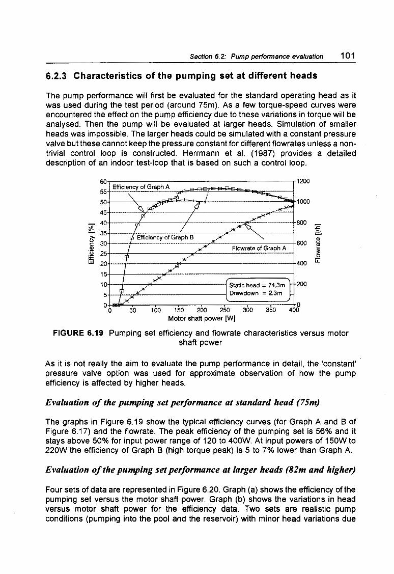
Univers
ity of
Cap
e Tow
n
Section 6.2: Pump perfonnance evaluation 101
6.2.3 Characteristics of the pumping set at different heads
The pump performance will first be evaluated for the standard operating head as it was used during the test period (around 75m). As a few torque-speed curves were encountered the effect on the pump efficiency due to these variations in torque will be analysed. Then the pump will be evaluated at larger heads. Simulation of smaller heads was impossible. The larger heads could be simulated with a constant pressure valve but these cannot keep the pressure constant for different flowrates unless a nontrivial control loop is constructed. Herrmann et al. (1987) provides a detailed description of an indoor test-loop that is based on such a control loop.
60 1200
55
50 1000
45
~ 40 800 :c 35 =.
>- ,Y1(· Q) (..') 30 600 cu c
_.,, .. /•( Q) Flowrate of Graph A .... ·u 25 ~
= 0 w 20
)ii'!'.
400 u::
15 )!¥.*
10 200 Static head= 74.3m 5 Drawdown = 2.3m
0 0 0 50 100 150 200 250 300 350 400
Motor shaft power [W]
FIGURE 6.19 Pumping set efficiency and flowrate characteristics versus motor shaft power
As it is not really the aim to evaluate the pump performance in detail, the 'constant' pressure valve option was used for approximate observation of how the pump efficiency is affected by higher heads.
Evaluation of the pumping set performance at standard head (75m)
The graphs in Figure 6.19 show the typical efficiency curves (for Graph A and B of Figure 6.17) and the flowrate. The peak efficiency of the pumping set is 56% and it stays above 50% for input power range of 120 to 400W. At input powers of 150W to 220W the efficiency of Graph B (high torque peak) is 5 to 7% lower than Graph A.
Evaluation of the pumping set performance at larger heads (82m and higher)
Four sets of data are represented in Figure 6.20. Graph (a) shows the efficiency of the pumping set versus the motor shaft power. Graph (b) shows the variations in head versus motor shaft power for the efficiency data. Two sets are realistic pump conditions (pumping into the pool and the reservoir) with minor head variations due

Univers
ity of
Cap
e Tow
n
102 Chapter Six: Array, pump and Miffek system performance
to drawdown in the borehole. The other two sets are simulated with the pressure valve and have head variations of up to 1 Om. Nevertheless, the conclusion can be drawn that the pump efficiency increases with increasing head. This is more noticeable at high power input than at lower power. This is to be expected as the pump can be installed up to a depth of 150m.
10~-------------,
..................... 65+-------..,,,., ... .,,. ... _. ......... =--..... .w~---
/____....-...__ 80··------~-·J~,'~~'::::::::::.......:.;;;~-~:t-.::----l
••
/, """-...,,_ ........... '1
'<ft. 55+---~fi;c__' ______ -............._~--1 ~ ~/I '=
·~ 00+--_/._..,,,~~-----·-----1
ffi 45
40,+-------------1
~.-!------------~
3000 100 100 200 200 300 ~ 400 400
Motor shaft power [W]
(a)
110
105
100
- 95 .s 11 90 a> I 85
.:«" ..... •
-
..... .. ............ ..+
....... ...., ............. ......- ~ .. \. .......... ...... _ ..
~· .... x···· Head variations due to pressure valve
~ \ - ~
~ Head variations due to drawdown
80
75
70 00 100 100 200 200 300 ~ 400 400
Motor shaft power [W]
(b)
FIGURE 6.20 (a) Pump efficiency over a range of heads; (b) head variations (key to Graph a)
The pumping set reaches an efficiency of 67% at a head of 108m. As the head decreases to 1 OOm the efficiency reduces to 54%. This reduction in efficiency is related to low input power levels rather than a decrease in head.
6.2.4 Pumping set losses
The aim of this section is to evaluate all the losses that occur in the pumping set. These are consequently subtracted from the pumping set performance data to yield the efficiency of the pump itself. The resulting data is used for comparison to the manufacturers specifications. The discussion is based on the diagram of Figure 6.12.
Mechanical losses
These can be divided into V-belt transmission losses, discharge head losses (bearings, anti-reversing mechanism and gland packaging) and transmission shaft friction losses. An attempt was made to measure the V-belt transmission losses with the method proposed in the test methodology. This was unsuccessful. The slip is most probably too small and is flooded by the measurement error. The discharge head losses and the shaft friction losses were not measured.
Gosnell (1991) estimated these latter losses to be 7% and Payne (1986) estimated these losses to be 12%. For this evaluation they will be assumed to be 10%. Since the pump is usually treated as a single unit (motor output to water delivered) an error in this estimation does not effect the evaluation of any of the system components.

Univers
ity of
Cap
e Tow
n
Section 6.2: Pump performance evaluation 103
Hydraulic losses
These losses are equivalent to the dynamic head which is the sum of the friction head losses (friction of the water on the inside of the pipe wall) and velocity head losses (local velocity losses due to valve, bends, contraction and other general obstructions). The dynamic head losses increase with the square of the flowrate. These losses occur in the rising main water pipe, in the discharge head outlet and in the post discharge head pipe network.
The rising main water-pipe losses were not measured but rather evaluated from a graph supplied by Mono Pumps. It is a graph of the head losses in the rising main pipe as a function of the flowrate. The curve is slightly exponential. Head losses increase from zero meter at zero flow to 1.4m at 10001/h, for a head of 75m.
The discharge head outlet losses were assumed to be negligible since the installation used 32mm pipe which does not result in significant head losses due to pipe contraction since the flowrate is low.
The post discharge head pipe network losses include velocity head losses due to a number of bends in the network and due to the Kent volume flowmeter and due to the head losses as a result of friction. These losses were measured but no significant pressure increase above the static head could be measured. Hence these were considered to be negligible.
6.2.5 Comparison to pump specifications
The graphs shown here were extracted from the specification sheet of the pump (appendix A 1.3). The specifications are presented slightly differently in the sheet. They have therefore been processed.
The performance of the pump has been isolated for this subsection by taking account of the mechanical and hydraulic losses (section 6.2.4) which occur in the pumping set.
Figure 6.21 shows the flowrate and torque at 75m as they were measured and as they are specified. The measured flowrate is slightly lower than the specified flowrate. At 1 OOOrpm this difference evaluates to be 5.8% lower than the specified value. This decreases to zero at 150rpm. I find this difference plausible and acceptable. Besides the uncertainty in the flowrate the assessment of losses may not be accurate enough. If they have been underestimated then the pump performance will evaluate lower.
The absolute uncertainty in the flowrate data is:
uabs (Q)200-+10001/h = 6.1 %
The largest ·uncertainty is introduced through the calibration of the volume flowmeter. This had to be calibrated by running water into a bucket whose markings had to be aligned with the water-line. The volume flowmeter itself had an accuracy of about 2%.

Univers
ity of
Cap
e Tow
n
1 04 Chapter Six: Array, pump and Miltek system perfonnance
1400 6.0
+. specified torque specified flowrate
1200 ........
5.5 ....... ..
5.0 1000
'.C' \\,\ 'E =. 800 \ 4.5 ~ Q) measured
~ flowrate Q) ::i
~ 600 .f
4.0 e-u:: {:.
400 . ·:;~........... . ............. 3.5 ~*')ili··~°*W··~·~ .................
200 3.0
0 2.5 0 200 400 600 800 1000 1200
Pump speed [rpm]
FIGURE 6.21 Measured torque and flowrate compared to specifications
The torque curve deduced from the specifications does not seem to be plausible. It is unrealistic to require such a large torque at 200rpm (nearly double the running torque) and then decrease to a minimum torque at 1000rpm. One would expect the torque to increase steadily from low operating speeds to high operating speeds due to the effetct of the self-compensating stator. The principle behind the selfcompensating stator is to reduce the torque on start-up. However, the stator does not compensatE~ immediately after start-up but requires a pressure head from the static head and from the flowrate. As compensation takes place, the torque will increase.
50
~ 40
~ c: Q) '() 30 = UI
20
10
0
measured efficiency
• .+ 250
-1-~-;:.:__~~-/-~~~~~~--,,~·~·*_ ... _ .. -~ .... ~ .. -~ .... ~·"~-t-200 i 4-~l--~~-T'-~~~~~ .... .__---'~~~~~--t-150 s
w,::? calculated output power ~ 4--f-~~+-~~-,,o~"~~-"~~~~~~~~~~T100 Q * ......
* . ..t'__...,..· --- s?ecified output power ;.i.:• • ..er-- 50
+a.--r-~---r-~--.~--,~~.,.-~,.-~-r-~---r-~--t-O
50 1 00 150 200 250 300 350 400 450 0 Pump input power [W]
FIGURIE 6.22 Measured pump efficiency and out put power characteristics compared to the specifications
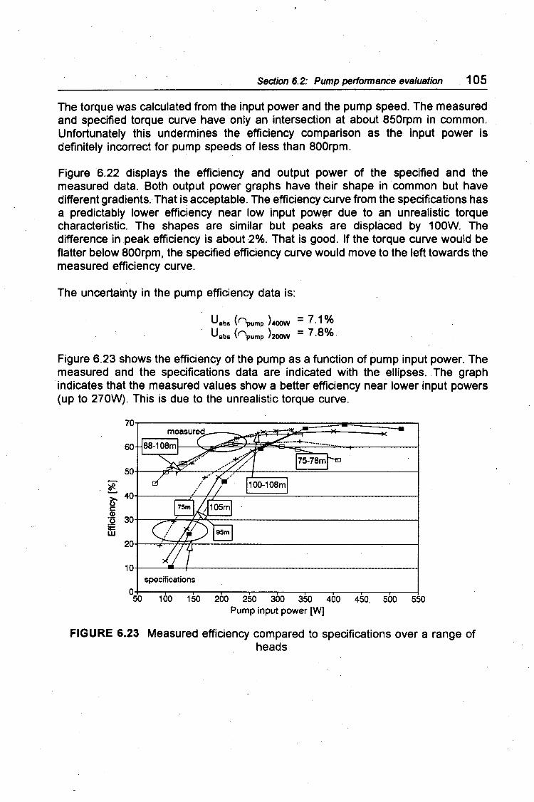
Univers
ity of
Cap
e Tow
n
Section 6.2: Pump perfonnance evaluation 105
The torque was calculated from the input power and the pump speed. The measured and specified torque curve have only an intersection at about 850rpm in common. Unfortunately this undermines the efficiency comparison as the input power is definitely incorrect for pump speeds of less than 800rpm.
Figure 6.22 displays the efficiency and output power of the specified and the measured data. Both output power graphs have their shape in common but have different gradients. That is acceptable. The efficiency curve from the specifications has a predictably lower efficiency near low input power due to an unrealistic torque characteristic. The shapes are similar but peaks are displaced by 1 OOW. The difference in peak efficiency is about 2%. That is good. If the torque curve would be flatter below 800rpm, the specified efficiency curve would move to the left towards the measured efficiency curve.
The uncertainty in the pump efficiency data is:
Uabs {~ump }4oow = 7 .1 % Uabs {~ump )2oow = 7 .8% ·
Figure 6.23 shows the efficiency of the pump as a function of pump input power. The measured and the specifications data are indicated with the ellipses. The graph ·indicates that the measured values show a better efficiency near lower input powers (up to 270W). This is due to the unrealistic torque curve.
70 .. 60
50
~ 100-108m
~ 40
c: C1> ·5 30 = w
20
specifications o--~..-~..-~..-~..--~....-~..--~..--~..--~..------1
50 100 150 200 250 300 350 400 450, 500 550 Pump input power [W]
FIGURE 6.23 Measured efficiency compared to specifications over a range of heads

Univers
ity of
Cap
e Tow
n
1 06 Chapter Six: Array, pump and Miltek system perfonnance
6.2.6 Conclusion on the type of pump used
The self-compensating stator pump was originally designed for hand-pump applications up to a maximum speed of 200rpm (Payne 1986). In the opinion of Rob Waites it is therefore not suitable for PVP applications which usually exceed this speed. Mono Pumps though, sell this type of pump as a solar element for speeds up to 1200rpm.
Mr Waites suggested to rather use a standard moulded element pump like the Orbit 0102. The torque curve is a straight line and has no unstable areas. The starting torque would be higher but that can be overcome with intelligent start-up routines (not for the present Miltek DC converter).
80
70
60
J1.. Specified efficiency of Orbit 0101 ....... +····· +········+········-+····· r····· ¥e ••••••• ~
I I
~ 50
~ 40 c: Q)
·c:; = 30 w
20
10 4-1--_M_e_as::-::-u-:-re_d e_,ff=ic,,...,ien,......c-=-y -----i Static head = 75m
of MonoS2M
0 0 100 200 300 400 500 600
Pump input power [W]
FIGURE 6.24 Efficiency of the Mono S2M and the Orbit 0101 & 0102 pump
Figure 6.24 shows the specified efficiency of the Mono S2M pump, the Orbit 0102 pump, the Orbit 0101 pump and the measured data of the Mono S2M pump. The Orbit
. 0102 ean be installed to a depth of 150m. At 75m the efficiency curve is still rising. It does reach a good efficiency from 450W onwards (that is larger than 60%) but this particular system produces a maximum motor output power of 400W. This pump is therefore not suitable. The Orbit 0101 is designed for static heads up to 75m. It would therefore be operating at its pressure head limit. It shows an excellent efficiency (more than 70%) over most of its input power range (100W to 350W). This element would be an alternative to the present choice. Unfortunately its input power range is too narrow and it is operating at its maximum head. I am not sure what the effect would be if the pump would receive an input power of 400W and operated at heads larger than 80m.

Univers
ity of
Cap
e Tow
n
Section 6.3: Miltek system perfonnance analysis 107
6.3 Miltek system performance analysis
This is the PVP system that the prototype inverter systems will be compared with. It is a well established system which has proved to be reliable under long term running conditions.
The converter and the motor performance are analysed as separate components and as a subset of the complete system. Then the overall performance of the system and the subsystem is evaluated on an instantaneous and a daily energy efficiency basis.
System tuning
The system was tuned with regard to the operating point on the array and the optimum motor pulley size.
The fixed voltage point was set to about 91V. This was found to be close to the MPP at cell temperatures of 47°C (refer to Figure 6.8). Average cell temperatures were in the region of 40°C (windy) to 55°C (no wind) on a sunny day.
The choice of motor pulley was guided by three criteria (discharge head assembly pulley remained constant, being 247 pitch centre diameter):
• the converter should only enter the direct mode (where fixed voltage operation stops, but efficiency across the converter increases) close to the maximum daily irradiance level (estimated to be 1050W/m2 over the year) 1
• the pump speed at high irradiance levels should be maximised which in turn maximises the flowrate
• the start-up delay should be minimised
The first criterion will require the pulley diameter to increase (higher torque therefore higher converter current and therefore higher array-current-threshold before entering direct mode), the second criterion depends -on the motor efficiency at different torque levels and the third criterion will require the pulley diameter to decrease (less torque, less converter current and therefore earlier start-up). The last criterion should not be over-emphasised as the system uses a tracking array which means that system startup conditions can be reached earlier in the day (on clear days).
This criterion has been simplified. For true optimisation two effects have to be taken into account. One, the higher efficiency of the converter in direct mode but with reduced array output due to operation away from the MPP Qn direct mode). Two, the lower converter efficiency at lower array input powers. The threshold voltage at which the direct mode is to occur is evaluated by finding the point of minimum losses (of effect 1 & 2) over the period of a year for the particular site. This of course is not possible for lack of data prior to installation. In addition, this evaluation would be relatively tedious. It was therefore decided to remain close to the MPP of the array by selecting a pulley for which the direct mode would occur near higher irradiance levels.

Univers
ity of
Cap
e Tow
n
108 Chapter Six: Array, pump and Miltek system perfonnance
Figure 6.25 shows at what irradiance level the converter progresses into direct mode for different size pulleys. The pulley with a pitch centre diameter (PCD) of 112mm enters the direct mode at about 850W/m2 and the pulley with a PCD of 140mm does not go into direct mode at all. The best choice from this graph would be pulley 125 which just goes into direct mode.
From the point of view of power extraction out of the array, pulley 112 extracts 6.5% less power (at more or less the same irradiance level) than pulley 125 as it operates at an array voltage of 97V. Consequently it does not manage to reach the same speed as pulley 125. Similarly for pulley 118 although here the array power difference is 4.4%.
FIGURE 6.25 Array voltage as a function of irradiance for different pulley diameters
Pulley 125 and 140 have similar performance data. Taking the first (just going into direct mode) and the third criterion (early start-up) into account it was decided to choose the 125 pulley.
It was noted later that the transition into direct mode did not always occur at the same irradiance level but could occur 1 OOW/m2 earlier (temperature and load variations).· It also became apparent that start-up time-delay between the 125 and the 140 pulley is not very long, about 15min. Therefore a 140 pulley would also have been acceptable.
6.3.1 Co1nverter and motor performance
Efficiency at standard head (75m)
The converter starts operating at an input power of SOW as shown in Figure 6.26. The efficiency reaches 80 % at 1 OOW and then increases linearly to 97% at 520W.

Univers
ity of
Cap
e Tow
n
Section 6.3: Miltek system perfonnance analysis 109
The three percent losses at maximum input power (for this particular configuration) are due to conduction losses in the MOSFErs and due to power consumption in the control electronics. The switching losses are zero as the converter tias changed to direct mode (in direct mode the converter ceases to switch such that the array is directly connected to the motor).
100
90
80
70
~ 60 ~ 50 c: Q)
·c:; 40 = w 30
20
10
0 0 50
subset combination
100 150 200 250 300 350 400 450 500 550 Array power [W]
FIGURE 6.26 Miltek converter, motor and subset efficiency versus array power
The uncertainty in the converter efficiency data is:
U (n ) = 3.0% abs con SOOW
urel (neon >soow = 1. 7% Uabs (neon hsow = 4.3% U (n ) = 3.2% rel con 250W
The motor efficiency rises sharply at SOW array power from zero percent to 60% at 120W and then rises more slowly (with a decreasing gradient) to 80% at 520W. The subset efficiency rises above 60% at an input power of 180W and reaches a maximum at 77.6%.
The uncertainty in the motor efficiency data is:
Uabs (nmot )480W : 4.1 % U (n ) = 3.6% rel mot 480W
Uabs (nmot hsow = 5.6% U (n ) = 5.0% rel mot 250W

Univers
ity of
Cap
e Tow
n
11 0 Chapter Six: Array, pump and Miltek system perfonnance
The uncertainty in the subset efficiency data is:
uabs ('\ubset )soow = 4.4% urel ('\ubset )soow = 3.6% Uabs (l\ubset hsow = 5.9% urel (l\ubset hsow = 5.4%
The converter efficiency is quoted at 98%. That will be at full load which is 14A and 120V and most probably in direct mode. Under full load conditions and in direct mode the converter is likely to be more efficient due to the constant losses (for example control electronics) becoming smaller in relation to the total power processed. Therefore tlhe measured maximum efficiency of 97% indicates that the converter lives up to its specifications in direct mode. This specification however is not very informative,, since when the controller is performing its fixed voltage operation function, conversion efficiencies are lower than in direct mode, while in direct mode the cessation 01f voltage tracking can imply reduced array efficiencies through dev(ation from the MPP voltage.
The motor 13fficiency reache,s a maximum of 80%. Although the specifications did not specify the efficiency literature suggests that DC motors generally have an efficiency of 75 to 85%.
Efficiency at higher heads
The load on the pump was increased from the usual 75m head to 82m (pumping into a different reservoir), to 88 - 87m and to 100 - 107m where the last two were simulated with a pressure valve. The effect on the efficiency for the con~erter (Graph a) and the motor (Graph b) is shown in Figure 6.27.
82
~ ~+-~~~-~~_.::::..""="-:?~F-""if!=-~-j 80 ~ ~ ~+-~~~-~~--?~~~;.._~~-i
c: ·~ ~.i.-~~~-~.,,c..,A--6-4'--~-"'<"~~~-1 !tij ~ ~+-~~--,·~'--~~~~~~~-1
t: ~ ~+-~~r"--~~~~~~~~~-1
8 ~+--1-~~-~~~~~~~~~-1 ~+----.-~...-----.-~..----.-~..----.-~..--i
100 150 200 250 300 350 400 450 500 550 Array power [WJ
(a)
[ 78
~ c: Q) ·o i .... 0 0 :::!:
76
74
72 100m -107m
70
~ 00 150 200 250 300 350 400 450 : 500 550 Converter output power [WJ ,
(b)
FIGURE 6.27 (a) Converter efficiency and (b) motor efficiency over a range of heads

Univers
ity of
Cap
e Tow
n
CIJ
Section 6.3: Miltek system performance analysis 111
The converter efficiency tends to decrease with a larger load on the motor. The reason for this is larger conduction losses as more converter current is required to generate a higher torque for the pumping set. The motor efficiency at higher heads is lower at low input power. The graph gives the indication that the efficiency of the motor improves for higher heads as the input power increases in relation to the efficiency at the standard head (75m). That would make sense as the motor is operating under partial load conditions. The output is rated at 750W and the output power here is about half of that. One would therefore expect the efficiency of the motor to increase for larger loads and increased input power.
Characteristic converter and motor curves
These are shown in Figure 6.28 where the converter current and the pump torque are displayed as a function of array power (Graph a). The adjacent graph (b) shows the converter output voltage and the pump speed. The graphs show the proportionality that exists in DC drives between their electrical and their mechanical quantities.
5.5 100 1000
90 900 ?r 5.0
~ 80 .Q o!I 'E ~ ::::> 0
(jj t: CIJ
~ 0 0
CIJ 70 4.5 D>
Cll 60 600 .s::: 0
4.0 > 50 500
/ ...... .... CIJ
40 400 t: CIJ
3.5 > 30 300 c pump torque
0 0 20 200
3.0 [N.m] 10 100
2.5 0 0 0 100 200 300 400 500 0 100 200 300 400 500
Array power [W] Array power [W]
(a) (b)
FIGURE 6.28 Characteristic converter and motor (referred to pump) curves
6.3.2 Array operating point characteristics
The control algorithm is implemented in hardware. The algorithm maintains a fixed voltage point by controlling the motor speed which it does by switching the array voltage with a pulse-width modulation scheme.
Figure 6.29 shows the graphs of the array voltage and the array current. The voltage stays within one volt of its fixed voltage point until about 950W/m2 (also note the ADC resolution which is amplified times thirty here). The converter progresses to direct mode where the voltage rises sharply (relative to the fixed voltage point) and the gradient of the current decreases slightly. That is due to the IV characteristic of the array. At this point the array current is large enough to supply the motor directly and is therefore able to maintain the torque that the pump requires.
'E a. .=.. "i
CIJ a. "' a. E ::::> a..

Univers
ity of
Cap
e Tow
n
112 Cf1apter Six: A"ay, pump and Miltek system performance
>~ ,._ .. Cl) CD ttl =~ ~ ~ .... .... <
96
95
94
93
92
91
90 200 300
current
400 500 600 700 800 900 Plane of array irradiance [W/sqm]
FIGURE 6.29 Miltek converter fixed voltage operation (with direct mode). I
During dimct mode the converter cannot control the motor speed which is then controlled by the level of irradiance. It can just observe whether the array voltage drops below the fixed voltage point. If this happens the converter starts switching again and thus regains control.
0.5
........ 0.4 :> ........ (I)
2: 0.3 ::i (,)
;~ 0.2 c: 0 (I) O> 0.1 as .~ 0 > (I)
·a. 0.0 a. a:
-0~ 1
-0.2 0.0 0.2 0.4
Switching frequency: 2.78 kHz
0.6 . 0.8 1.0 1.2 1.4 1.6 Time [msec]
1.8
FIGURE 6.30 Ripple on the array voltage due to converter switching scherl'te
The input ripple due to the switching of the array voltage is shown in Figure 6.~0. It has a peak-to-peak voltage of 400mV. The loss that this would cause in array power due to operation away from the MPP is less than 0.02 %. But since the converter operates in fixed voltage mode the losses due to that (discussed in subsection 6.1.3) are far higher than the losses due to the input ripple. ·

Univers
ity of
Cap
e Tow
n
Section 6.3: Miffek system perfonnance analysis 113
6.3.3 General observations
Two aspects are discussed here, namely how the converter responds to dynamic conditions and the time-delay due to a linear start-up routine in the early morning.
Dynamic conditions
An appropriate test to evaluate the dynamic capabilities of a system is to apply a stepup or a step-down to the input. That was done by disconnecting one of the two strings that were connected in parallel (array configuration: 2x6). The input power to the converter was thus halved (step-down) or doubled (step-up) instantaneously relative to its previous input power. The test result is shown in Figure 6.31 .
7.....---.---.----,.--....--......-...... 8 6 ..---......----.-----.----,----.~1100
r----+--r1000 ~ converter current ~ay cur ent
~ 6 \ i\1 c i i}., ig 5 -------- ! r-o-""~-.,,,.,_ -=1-::J --------- _______ }
current 7 -
5 --------'E ~ 6 ~ u --CD 4 /""' t:: / ~ a / I
ID ::J
5 ~
c l!! ... ::J u
4 800 l 700 !II
a. c J.---+--+---' .·., 0 - 3 8 \ tore ue 2 : , ... ___ ----oa --------\ j
~ a. 4 E ... ...
::J <( 600 § >- : --------- --------~ 1 ,.,,.''
<( \ ,/ ,_, 3
0~0--.---+10-.--~+-~~~---.......-~+--....-+oo--+2
Time [sec]
(a)
a. 2 500
1 ~0-.--+10--..--+~---.......-~+--....-~+-......-~oo--+400
Time [sec]
(b)
FIGURE 6.31 Response of the subsystem to an array-current step input
Both graphs display the step-down and the step-up of the array current (solid line). Graph (a) also shows the converter current and the pump torque. Both curves drop rapidly but then increase logarithmically to the torque required by the pump and the current required by the motor under the new steady state conditions. The transition of the converter current from the rapid decrease to the logarithmic increase is very sharp which shows how fast the converter responds. The transition for the pump torque is smoother. The same can be observed for the step-up. It takes the system 11 sec to settle to a new steady state value. Graph (b) shows the pump speed in addition to the array current.
System start-up
The start-up of the PVP system depends on the ability of the converter to generate a large current at its output while the input current is still very small. Figure 6.32 shows the conditions at start-up as a function of time. This is the first start in the morning.
a.

Univers
ity of
Cap
e Tow
n
114 Chapter Six: Array, pump and Miltek system perfonnance
The non-zero pump speed in Graph (a) indicates when the start-up occurs, here at thirteen and a half minutes on the horizontal axis. The array current has a value of 0.88A and the array power has a value of SOW. The minimum power required from the array to kee1p the pump turning was measured to be 47W at 0.52A (measured as the array power decreases). From the graph this condition occurs at about 1 min. It follows therefore that the system could have operated already 12min earlier if it had employed a non-linear start-up routine where it would use the energy in the input capacitors to overcome tl1e break-away torque of the pump. The gain would be minimal, at the rate of irradiance increase shown in the graph, and in general the proportion of daily irradiation received between 50W/m2 and 80W/m2 is insignificant.
'E a,....------------~160 z_ 1 140 ~ CD 6 .. .,,,.l 120 'E :I
100 .§:: e- 5 !"•I
0
0 0 2 4
-GO 4 'E !!! ... 3 :I u
6 8 10
' 0.2 j pump i speed . 0.0
12 14 16
... 2 CD t:: CD
E: 8 0
0 2 4 6 8 10
Time (min] Time [min]
00 ~
FIGURE 6.32 System status prior to start-up
80
60
40
speed{ 20
0 12 14 16
Graph (b) shows the converter current and the pump torque. They increase more or less linear!)' after the first minute. The graph shows that the running torque is a lot lower than the start-up torque and the build-up to the start-up torque.
6.3.4 Syt:~tem performance
The aims of this subsection are to present the data of the Miltek PVP system and subsystem instantaneously and to present it on a daily basis for different amounts of daily solar irradiation. The daily energy efficiency of the components, the subset (controller and motor), the subsystem and the system and the volume flow are presented for standard solar days from 2kWh/m2/day to 8kWh/m2/day. The emphasis in this subsection is on the shape of the graphs more than the performance values that the S)rstem achieves. The latter will be discussed in more detail in the comparativ~~ chapter (chapter ten).
In addition, a solar irradiance profile for a single-axis tracking array has been generated, based on the solar irradiance profile in Figure 6.1 O. It is referred to as a tracking solar day. The system performance for a standard solar day and a tracking solar day will be compared.
"O
* a. Ill a. E :I
Cl.

Univers
ity of
Cap
e Tow
n
Section 6.3: Miltek system performance analysis 115
Instantaneous performance
The graphs in Figure 6.33 represent the system and the subsystem performance with corresponding flowrate.
The system efficiency reaches a maximum of 4.5% from 700W/m2 to 950W/m2 and then decreases to 4.2% at 1060W/m2
. The flowrate increases in a straight line in the 700W/m2 to 950W/m2 region. The gradient then reduces (as the efficiency reduces) and it reaches a peak value of 9501/h at an irradiance level of .1060W/m2
.
The subsystem efficiency reaches a maximum of 42%. It remains above 40% for array powers of 320W to 480W.
5.0 1000 50 1000
4.5 s stem
45 efficiency
~ 40 800 'ii 4.0 800
~ 35 ;: 3.5 § c (.)
CD 600 c 3.0 600 ·c; 30 CD CD Ii 25
·c;
Ii 2.5 iii .... E
E 2.0 400 ~ CD 20 400 CD u:: 1ii 1.5 *' 15 >- .0 200 Cf) 1.0 200 ::I 10
0.5 Cf)
5
0.0 0 0 ·o 200 400 600 800 1000 0 100 200 300 400 500 600
Plane of array irradiance [W/sqm] Array power [WJ
(a) . (b)
FIGURE 6.33 (a) Miltek system performance and (b) subsystem performance
The shape of the efficiency curves are similar in the upper half of the operating range. They both model the pump efficiency curve quite well in that region (refer to Figure 6.19), including the non-smooth section of the graph at 500W/m 2 to 650W/m 2 and 230W to 300W respectively which is due to the torque characteristic of the pump (refer to Figure 6.15). The first half of the system efficiency curve resembles a straight line whereas the subsystem efficiency has a more logarithmic curve (similar to the pump efficiency curve again).
The uncertainty in the system efficiency data is:
LJabs (l\ys )10SOW/sqm : 12.0% LJrel (l\ys )10SOW/sqm = 6.9% u (r.. ) = 15.7% abs · 'Sys 750W/sqm u (r.. ) = 9.4% rel · 'Sys 750W/sqm
I
'.C =:. CD iii
~ u::

Univers
ity of
Cap
e Tow
n
~
116 Chapter Six: A"ay, pump and Miltek system performance
The uncertainty in the subsystem efficiency data is:
Uabs (f\ubsys )soow = 6.6% urel (f'"'\ubsys >soow = 2.5% Uabs (f\ubsys }350w = 6. 7% u (r-. ) = 2.8% rel · 'Subsys 350W
The uncertainty in the flowrate data is:
Uabs (Q hoo _. 10001/h = 6.1 % urel (Q ">200 _. 10001/h = 2.2%
The subsystem efficiency proves to be the most reliable data for comparison since the absolute efficiency only reaches 6. 7% at two thirds of the input power. The system efficiency is largely dominated by the errors that can occur in the pyranometer.
Daily energy efficiency performance
The profile of the standard solar day (SSD) and tracking solar day and the method of calculation that was used to derive the data that follows below are presented in appendix AS.
100
90
~·~-----------:----, subset converter - 70,~---------==---=====1 ~
__ _.:..----
v- - motor ~
~ c: 70 Cl> ~
~ ~1+-----:::::--=--------i c: -~ 50,~_,,....::;_ __________ -1
·c:; ~
ffi 50 v !E
w ~1t---------=:::::::::::=====:::::j ~
v e> ~ pump ~ subsystem
~ ~+----::::--=--------1 c: Cl>
in ~ w ~+-:.,,..,C...-------------1 ~
~ 10.f---------------; array ~ ~ 0 10
02 3 4 5 6 7 8
0~2----..3--4..---~5--6..---~7---!8
Standard solar day [kWh/sqm/day] . Standard solar day [kWh/sqm/day]
(a) (b)
FIGURE 6.34 Miltek system daily energy efficiency (a) system components and (b) subset and subsystem
The daily energy efficiency (DEE) of the components is displayed in Graph (a) of Figure 6.34. The array maintains an efficiency of more than 10% from 2kWh/m2/day to 8kWh/m2/day (the instantaneous array performance data was only used from 600W/m2 to maximum irradiance levels, below 600W/m2 was assumed to be constant since data in that region was unreliable as discussed in section 6.1 ). The DEE of the converter progresses from steeper to flatter gradients but is still rising at 8kWh/m2/day having reached a value of 94.3%. The motor reaches a nearly constant value at 77% with little tendency to increase. The DEE of the pumping set reaches a peak of 54.4%
I
•
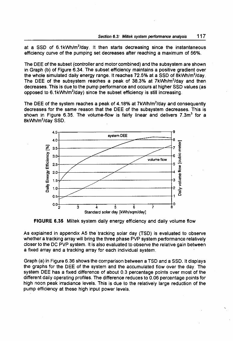
Univers
ity of
Cap
e Tow
n
Section 6.3: Miltek system perfonnance analysis 117
at a SSD of 6.1 kWh/m2/day. It then starts decreasing since the instantaneous efficiency curve of the pumping set decreases after reaching a maximum of 56%.
The DEE of the subset (controller and motor combined) and the subsystem are shown in Graph (b) of Figure 6.34. The subset efficiency maintains a positive gradient over the whole simulated daily energy range. It reaches 72.5% at a SSD of 8kWh/m2/day. The DEE of the subsystem ·reaches a peak of 38.3% at 7kWh/m2/day and then decreases. This is due to the pump performance and occurs at higher SSD values (as opposed to 6.1 kWh/m2/day) since the subset efficiency is still increasing.
The DEE of the system reaches a peak of 4.18% at 7kWh/m2/day and consequently decreases for the same reason that the DEE of the subsystem decreases. This is shown in Figure 6.35. The volume-flow is fairly linear and delivers 7 .3m3 for a 8kWh/m2/day SSD.
....... ~ ~ c: Q) ·c;
ffi e> Q) c: w ~ ·ca 0
4.5
4.0
3.5
3.0
2.5
2.0
system DEE +-~~~~~~~~~~-'--=--"""""";;__~~~---t8 "\:"
jg +-~~~~~~~-,.~~~~~~~~'"".:7"""'-T7 ~
+-~~~~-7"::;._~~~~~~~""'7""---~~---t6 ~ ::I (.)
+-~~~~~~~~~~-;o"'--~~~~~--r5 .........
~ 4 ;:: +-~~~~~~~~'?"""-~~~~~~~~--r Q)
E 1.5 .-l.l-~~~~~---,,....::;_~~~~~~~~~~--r3 ::I
~ '+-~~~,,..c-~~~~~~~~~~~~~--i-2 ~ 1.0
0.5
0.0 +-~~--r--~~-.-~~--,-~~---r~~--,~~---rO 2 3 4 5 6 7 8
Standard solar day [kWh/sqm/day]
·ca 0
FIGURE 6.35 Miltek system daily energy efficiency and daily volume flow
As explained in appendix AS the tracking solar day (TSO) is evaluated to observe whether a tracking array will bring the three phase PVP system performance relatively closer to the DC PVP system. It is also evaluated to observe the relative gain between a fixed array and a tracking array for each individual system.
Graph (a) in Figure 6.36 shows the comparison between a TSO and a SSD. It displays the graphs for the DEE of the system and the accumulated flow over the day. The system DEE has a fixed difference of about 0.3 percentage points over most of the different daily operating profiles. The difference reduces to 0.06 percentage points for high noon peak irradiance levels. This is due to the relatively large reduction of the pump efficiency at these high input power levels.

Univers
ity of
Cap
e Tow
n
118 Chapter Six: A"ay, pump and Miltek system perfonnance
M 0 300 400 500 600 700 800 900 1000 1100
Noon peak irradiance (W/sqm] ~ 400 500 600 700 800 900 1000 1100
Noon peak irradiance (W/sqm]
(b)
FIGURE 16.36 Tracking solar day and standard solar day for Miltek system DEE and volume flow: (a) performance and (b) percentage of TSO over SSD
Graph (b) shows the percentage difference between the SSD and the TSO by using the SSD as the base value and evaluating the percentage value by which the TSO exceeds the SSD. The difference between the TSO and the SSD becomes larger as the noon pE~ak solar irradiance decreases. At 11 OOW/m2 daily peak irradiance the DEE of the system under TSO conditions exceeds the SSD condition by about 1.5% whereas the volume-flow exceeds it by about 28%. These values increase as the energy content of the different profiles decreases. At 800W/m2 daily peak irradiance the TSO DEE of the system exceeds the SSD DEE by 7 .5% and the volume flow by 36%. The shape of these two graphs is as expected since the efficiency at lower irradiance levels is poorer and the SSD.
E' 1200 CT
.!!!. ~ 1000 Q) (.) c Ill 800 ] :; 600 Ill :g_ c 400 8 c ~ 200 f!
~ 0
J Site: Windhoek l Fixed array: 20deg tilt
' - - ,_ ,_ ,_ ,_
,_ ,..._ - ,_ ,__~
- .--[;:'. - ,_ ~ [;:'.
~ ,_ ,_ ,_ ,..._ ,_
~ Jan Feb Mar Apr May Jun Jul Aug Sep Oct Nov Dec
Month
FIGURI: 6.37 Average noon peak irradiance on a tilted surface at Windhoek
Figure 6.37 shows the average noon peak irradiance levels received at Windhoek on a 20° tilted surface over a year. The noon peak irradiance was calculated from long term recordings of the global and diffuse irradiance components using the program Solar Tilt (Cowan 1992).

Univers
ity of
Cap
e Tow
n
Chapter Seven
SOLVO SYSTEM PERFORMANCE ANALYSIS
The chapters on the prototype inverters (chapters seven and eight) each stand on their own and can be read independently of one another. Because of this there is a small amount of duplication with the result that some introductory paragraphs are the same or similar.
This chapter presents and discusses the Salvo inverter and motor efficiency, the steady state array operating point characteristics, the dynamic array operating point characteristics, the voltage to hertz relation, the control algorithm characteristics and general observations on the system. This is followed by the instantaneous system and subsystem performance evaluation and by the daily energy efficiency evaluation of the components and the system.
The derivation of the absolute and relative uncertainty in the acquired data is presented in appendix A3.6. The derivation of the stated uncertainty in the efficiency data is given by an example in appendix A3. 7. All uncertainties are stated as a plusminus percentage of a full-scale reading.
System tuning
The system was tuned with regards to the array operating voltage (it is a fixed voltage point algorithm) and the pulley size. In addition two programs were available that contained different voltage to hertz relations, therefore had different start-up and different operating characteristics.
The voltage point was fixed to a steady state value of about 182V. This was found to be close to the MPP at cell temperatures of 47°C (refer to Figure 6.8). Average module temperatures were in the region of 40°C (windy conditions) to 55°C (no wind) on a sunny day during March to May.
The choice of motor pulley was guided by two criteria (the pulley of the discharge head assembly remained the same for all tests, being 247PCD):
• the inverter should be able to just reach its programmed maximum output frequency at the maximum irradiance level
• the start-up time delay should be minimised
The choice was between a pulley size of 85PCD (pitch centre diameter), 97PCD and 112PCD. The smallest pulley managed to reach its maximum output frequency (85Hz) before reaching the maximum irradiance level. The 112PCD pulley would delay the start-up due to slightly higher torque requirements from the motor and so it was

Univers
ity of
Cap
e Tow
n
120 Chapter Seven: Solvo system performance analysis
decided to choose the 97PCD pulley which nearly managed to reach the full output frequency ;at full irradiance making it the most suitable pulley.
Two programs with different voltage to hertz relations were generated using a TurboPascal program written by Hirschmann (1989b). The graphs are shown in Figure 7.1. One program had a linear relation between the voltage and the frequency with a voltage boost near zero hertz (referred to as the linear program) and one program had a square-root relation between the voltage and the frequency, also with a voltage boost near small frequencies (referred to as the log program). The square-root relation was adaptetd from Davies' (1992) dissertation and scaled to the output voltage range and frequency range of the Salvo inverter. This was not necessarily optimal but offered the most practical solution in the circumstances at hand during the field tests (which is where the voltage to hertz relations were programmed into EPROM's).
120...-~~~~~~~~~~~~~~~~~---,
logarithmic Volts to Hertz:
.s 40 Q) c:
linear
~ 20+.-:::::~-H-l---i-+--l-~-+-~-t-~-+-~~+-~~-+--1
11 s i I . i :.!14 Gead5. !7 !B l9 10 ... 12 1,13 · ,15
o~~~·w·_;_·~·~·~,..;..-__..:....,.--'--.-~~· ,--~~·~-,-____.-; 0 10 20 30 40 50 60 70 80 90
Frequency [Hz]
FIGURE 7.1 Linear and logarithmic voltage to hertz relation
The choice of voltage to hertz relation was guided by two criteria:
• the program should drive the inverter-motor subset most efficiently resulting in an optimised pump speed over the full operating range
• the program should result in as early a start-up as possible
It was found that the subset efficiency with the log program at low array power (1 OOW to 200W) was better by an average of 6% than the linear program. In the midoperating region (250W to 350W) the linear program proved to have a better subset efficiency t11an the log program, the average difference being 3%. Towards the full operating input power (350W to 550W) the efficiencies were similar. The log program resulted in a slightly higher pump speed (15 rpm on average) than the linear program. It was also found that the log program operated better in the low input power region. It runs more smoothly and has a lower start-up and cut-out threshold. Therefore the choice was for the log program.

Univers
ity of
Cap
e Tow
n
, Section 7. 1: Inverter and motor performance 121
7 .1 Inverter and motor performance
This section deals with the inverter, the motor and the subset efficiency at standard and simulated higher head as well as with the characteristic inverter and motor curves.
7.1.1 Efficiency at standard head (75m)
The inverter efficiency includes the losses due to the dynamic array operating point characteristics (as will be discussed in section 7.3). It does not include the losses due to steady state operation away from th·e MPP. It also does not include the mismatch losses between the inverter and the motor which are caused by the harmonics in the current waveform. These losses are included in the motor efficiency.
The uncertainties in the efficiency results are stated at the end of each discussion.
The inverter efficiency is evaluated over an input power range of 1 SOW to 540W. The inverter starts operating at an input power of about 11 OW. Figure 7 .2 shows the first data point at an array power of 1 SOW with an efficiency of 31 %. The efficiency rises to 84% over the input power range from 1 SOW to 360W. It then stays constant at 84% up to 540W.
~
901--~~~~~~~~~~~~~~~~~~~--,
motor inverter 801+,~~---'....,,_~~~~~-7';:~,,...8"""--~~~~~--,
101l-~~~~~,--~~:!f::::l=::!:::±:::::::!=:l:::::i==i-;--+-t-d::::l~~
so.J-~~~~~~-l,.,(.:__~~~-:7:"~~~~~,.._,._'--1
~ 50 c -~ 40.+-~~~~--iF+--ef~~~~~~~~~---'~~-.
~ ~~ w 30-1-~~~~_i,;.i_-1--r-~~~~~~~--:--:-co~m~b~in=m~io=n,--i'
0 0 50 100 150 200 250 300 350 400 450 500 550
Array power [W]
FIGURE 7.2 Salvo inverter, motor and subset efficiency versus input power
The uncertainty in the inverter efficiency data is:
U (n ) = 8.4% abs inv SOOW
urel (ninv )soow = 5.3% uabs (ninv )2sow = 19.2% urel (ninv )2sow = 12.3%

Univers
ity of
Cap
e Tow
n
122 C/Japter Seven: Salvo system performance analysis
The inverter losses decrease from about 1 OOW at 150W input power to about 65W and then increase to 85W at 540W input power as can be seen in Figure 7.3. The losses can be divided into constant and varying losses. The constant losses consist of the power supply losses (comparatively small since the inverter uses a switch-mode power supply), microcomputer power requirements and the drive circuit power requirements. The drive circuit is quite intricate as the PWM signals are modulated with a carrier, then amplified in two stages and coupled across HF transformers. This will require more power than conventional drive circuits. The constant losses have been measured to be about 18.6W (216V x 0.086A) but will be taken as 20W.
100
90
80
70
[ 60 Ul Ul .Q
~ ~
50
40
30
20
10
0
-
\ ~ ~
~ .r - ~
0 50 100 150 200 250 300 350 400 450 500 550 Array power [W]
FIGURE 7.3 Salvo inverter losses
The varying losses are the switching losses and the conduction losses. The switching losses can be calculated (Hexfet Power MOSFET Designers Manual 1987: 1-141) from the linearised current switching waveform (which has not been sampled on the oscilloscope). The essential parameters are the array voltage (here constant), the line current and the time base. This results in the energy lost during switch-on and switchoff (it is likely to be very small since the current ripple on a high switching-frequency generated current waveform is small). This value is multiplied by the switching frequency to evaluate the losses in one phase. Therefore the switching losses vary -linearly with changes in switching frequency. The switching frequency of the inverter changes within a major gear since the inverter changes the output frequency through changing t11e switching frequency. The average switching frequency within a major gear has been programmed to decrease from about 15.5kHz at low fundamental frequency (1 OHz to 30Hz) to 11.2kHz at high fundamental frequency (70Hz to 85Hz). The tendency is therefore for the switching losses to decrease.
The conduction losses in one leg of the three phase bridge are a function of the onstate resistance of one MOSFET and the line current that is passing throµgh it as well as the power dissipated in the source-drain diode of the other MOSFET (which is turned off). These losses can be calculated (Hexfet Power MOSFET Designers Manual

Univers
ity of
Cap
e Tow
n
Section 7.1: Inverter and motor performance 123
1987: 1-145) if the line current, the power factor, the on-state resistance and the diode forward voltage-drop are known. The conduction losses are varying because the torque requirements of the pump are not constant. Therefore the conduction losses will somewhat follow the shape of the line current with a minor peak at 250W input power and another higher peak at the ~nd of the operating range.
None of the varying losses have been measured but the conduction losses can be calculated as mentioned. That will give an idea of the switching losses. The conduction losses are equal to:
3 x (0.462 x pf x 12peak X R0500 + LF X 0.068 X lpeak X V50] = 9W to 14.BW
for pf = 0.4 (estimated), R0500 = 0.32Q, lpeak = 6A to BA, LF = 3 (load factor, from HEXFET manual) and V50 = 0.7V). The constant losses were measured to be 20W. Therefore the total losses excluding the switching losses would be 29W (low input power) to 35W (high input power). The switching losses would therefore have a magnitude in the range of 71W (at low fundamental frequency) to SOW (at high fundamental frequency) which is relatively high. The inverter losses have a low between 350W to 450W (that is, they are below 70W) which is where the line current is the lowest.
The occasional bumps in the curve will stem from the relatively large changes in voltage from one major gear to another, from variations in the switching frequency and from the load characteristics of the pump (see Figure 6.15).
The motor efficiency (Figure 7.2) rises sharply to 72% at an array power of 230W and remains there to the end of the operating range with a slight dip to 70%. The specifications for the motor are only available at 50Hz with input powers exceeding the operating range under which the motor was tested. Nevertheless, at 530Winput power (50Hz and line voltage= 70V) the specified motor efficiency reaches 75.6% and 73% for 11 OV line voltage. The motor therefore comes very close to the specifications, reflecting the low harmonic content in the current waveform since the inverter switches at very high frequencies. The motor dissipated very little heat which is an indication that the present harmonic energy was small. It is surprising though that the efficiency curve is so flat. One usually does not expect the motor efficiency to be good at low input powers. The motor was specifically designed for small power applications by GEC. I would not be able to explain why the motor exhibits such a good efficiency at low input power.
The uncertainty in the motor efficiency data is:
uabs (nmot }42ow = 9.2% U (n ) = 6.6% rel mot 420W uabs (nmot )2sow = 14.5% urel (nmot )2sow = 9.8%

Univers
ity of
Cap
e Tow
n
124 Chapter Seven: Salvo system performance analysis
The subset efficiency of the inverter and motor combined shown in Figure 7 .2 reaches 50% at 230W input power and reaches about 60% at 370W input power where it remains. The subset efficiency is the most important gauge in terms of the efficiency evaluation of inverter and motor for the following reason: Inverter efficiency can be increased by decreasing the switching frequency. This results in a higher current ripple on the line current with effect of increased motor heating and consequently a reduced motor efficiency. The aim is therefore to find the maximum efficiency of the combination as a function of the switching frequency if such a switching frequency exists. From a measurement point of view, the uncertainty in the subset efficiency is lower than the uncertainty of the inverter or motor efficiency.
The uncertainty in the subset efficiency data is:
uabs (r1subset )soow = 4.5% U (n ) = 4.2% rel subset 500W
Uabs (~ubset )2sow = 5.3% urel (nsubsel )2sow = 4.9%
7.1.2 Efficiency at higher heads
The result for the subset efficiency at different head is shown in Figure 7.4. Unfortunately only two sets of the acquired data were valid. The one head is at 75m and the simulated head is at 105m (by using a larger pulley).
~-"o ~:::. :... 50 ···---·----() c (I)
·u :e <O
20 - -···---··-------···-··-··-···--...... ___ ,,,, ______ , ___ , __ ,,,, ..
10-1--~~~~~~~~~~~~~~~~~..--~--i
150 200 250 300 350 400 Array power [W]
450 500 550
FIGURE 7.4 Solvo subset efficiency at one higher simulated head
The graph shows that the subset efficiency at higher head is lower in the low input power region but reaches the same efficiency towards the end of the operating range. The inverter efficiency decreases due to higher current requirements from the motor. This will result in higher conduction and switching losses which are a function of the current squared and the current magnitude and shape respectively.

Univers
ity of
Cap
e Tow
n
Section 7. 1: Inverter and motor performance 12 5
An improvement in the motor efficiency while operating along a new load curve (that is higher head, or different pulley size) is mainly dependent on how optimally it is driven by the inverter in terms of its voltage to hertz relation and harmonic content. A number of parameters have to be known to make a comment on this. However these are not available. ·
The inverter and motor efficiency are likely to improve if, for example, the array was doubled in size to 24 modules (two strings of 12 modules in series) since only the variable losses would increase assuming that a larger motor pulley would be used. The subset efficiency of the simulated higher head shows this trend in that it reaches the same efficiency at high input powers and would probably increase beyond the 75m subset efficiency if more power was available.
7.1.3 Characteristic inverter and motor curves
The characteristic curves of the inverter and the motor under these particular load conditions are shown in Figure 7 .5.
4.0 100 1000
'E ff. speed
-·-\~L. ____ :Z_ 3.5 ~
.J
.---------..___.___..-~torque .~ Cii ca
80 800 .....
~ 3.0 ~
'N ~ 60
.... ·
\ 600
.9 ~...=tf!ID
~current ca 2.5 ~ c:
-~ -........,
QI 40 400 :::> 'E ~ 5 2.0 CT
~ -.... 200 0 QI :a 1.5
QI t:: QI
20 slip
.c a..
1.0 100 200 300 400
Array power [W]
(a)
> ..s: 500 600
t • .. t++-i
0 0 100 200 300 400 500 600
Array power [W]
(b)
FIGURE 7.5 Characteristic subsystem curves: (a) Phase current and pump torque; (b) frequency, slip and pump speed
The inverter current follows the pump torque curve quite closely (graph a). The discontinuity at about 480W array power is due to a large change in inverter output voltage (from major gear 14 to 15).
The frequency (Figure 7.5b) follows a reasonably straight line (with a tendency _towards a logarithmic shape) and the slip between the inverter frequency and the rotor of the motor drops rapidly from 100% to 5%. The slip is 100% at 140W array power since·the rotor has not started turning yet. The pump speed curve has a similar shape to the frequency curve which is to be expected.
The inverter voltage has been omitted due to large measurement uncertainties.
'E ~ -0 QI QI a. U)
a. E :::> a..

Univers
ity of
Cap
e Tow
n
126 Chapter Seven: Solvo system performance analysis
7 .2 Steady state array operating point characteristics
The Solvo inverter offers one type of control algorithm namely fixed voltage operation (FVO). Under steady state conditions the average array voltage showed that FVO was implementod well as can be seen in Figure 7.6 .
....--------------------r3.5
-1----------~-----~------t-2.5 ...... ~
-1------------::,....i::..--------+2.0 c: ~ ::I 0 -1-----------,,..i:::------------+1.5 >-
~ ~ -1-----....,...::--------------+1.0 c(
+--:::>+<:::;__----------,--------;-0.5
-1---....--......--......---......---......---....---....---....----ro.o 400 500 600 700 800 900 1000 11 00
Plan.e of array irradiance [W/sqm]
FIGURE 7.6 Fixed voltage operation of Solvo inverter
This shows the average array voltage and the average current as a function of the irradiance. Towards low levels of irradiance the inverter loses its operating point and the array voltage decreases.
7 .3 Dynamic array operating point characteristics
The mean array voltage proved to remain close to the set-point to which it was tuned. However the instantaneous Voltage had quite a large movement about that mean value. As this could result in a diminished array output and can have a negative impact on the motor performance the effect of this array voltage oscillation is analysed here.
It is common for switch-mode inverters to have a ripple voltage on the DC-side Input which is due to the switching scheme employed by the inverter. The magnitude df the ripple is dependent on the switching frequency of the inverter (inversely related). Its frequency is the same as the switching frequency. However, the ripple discussed here (referred to as an oscillation voltage) is the result of the type of control algorithm implemented in the inverter (a detailed analysis of the control algorithm is in section 9.1 ). This section purely evaluates the impact of the oscillation voltage on the array performance and on the shape of the PWM inverter output signal. The effect of a larger input capacitance on the array voltage oscillation is also evaluated.

Univers
ity of
Cap
e Tow
n
Section 7.3: Dynamic a"ay operating point characteristics 127
7 .3.1 Shape of oscillation waveform
The typical oscillation waveform at the input to the Solve inverter is displayed in Figure 7.7. This waveform is riding on the mean array voltage as shown in Figure 7.6.
15
5
(\ f1 f\ r A ~ n I I I f' I\
\ ' I ,
v \ ~ ~
10
0
-5 I
-10
-15 v \J v -20 ~ v
0.0 0.2 0.4 0.6 0.8 1.0 1.2 1.4 1.6 1.8 2.0 Time [sec]
FIGURE 7.7 A typical array voltage oscillation waveform riding on 182Varr
The oscillation waveform has sine-wave characteristics. It has two distinctive waveforms that differ in amplitude and frequency. One waveform has a peak-to-peak amplitude of about 20V to 30V at a frequency of 3.8Hz and the other waveform has a peak-to-peak amplitude of 10V to 15V at a frequency of 7.6Hz (approximately double the other waveform). No statement can be made whether the one or the other . waveform occurs more or less often at particular operating conditions. The waveforms do not change significantly with changes in input power. The waveform can also contain a ripple at the switching frequency of the inverter. This occurs mainly near low input power levels. The amplitude of the waveform increases if the FVP is moved to the left of the MPP and decreases if the FVP is moved to the right of the MPP. The shape of the waveform remains unaltered.
7 .3.2 Array power losses
In order to assess the impact of the oscillation on the array output, the waveforms from above were superimposed on the steady state array operating point by using information of a characteristic ·array power curve. The method of calculation is described in appendix A6.
Figure 7.8 shows the result of this procedure. The two lines represent the two oscillation waveforms displayed in Figure 7.6. The peak-to-peak amplitude is varied by scaling the oscillation voltage amplitude. The operating point on the array is at MPP. Therefore the percentage power loss is zero at oscillation amplitude of zero. The windows display the most commonly found peak-to-peak amplitudes of the oscillation.

Univers
ity of
Cap
e Tow
n
128 Chapter Seven: Salvo system performance analysis
~ .... Cl>
~ O> c: ·2 'ai E ~ Cl> O> C'CI -c: Cl> ~ Cl> a..
100
99 MPP = 175V
98 Fixed voltage = 175V
97
96
95
94
,./"-..._ The most common // "' am litudes encountered
are in these windows
The two lines represent oscillation voltages captured at different
operating con it1ons ·· ....... ..
93+---.--.....,.--.,---r--~--r---.-----r-----ir------i 0 5 10 15 20 25 30 35 40 45 50
Peak-peak amplitude of oscillation [V]
FIGURE 7.8 Percentage of remaining array power versus a range of oscillation waveform amplitudes while operating (on average) at MPP ·
Power losses of half a percent for the small oscillation waveform and one-and-a-half percent for the large oscillation waveform can be expected.
100
~ 99
.... 98 Cl>
~ 97 C> c:
96 ·c: '(U
E 95 Cl> .... Cl>
94 O> C'CI c:
93 Cl> 0 .... Cl> a.. 92
91
MPP = 175V
The four lines represent oscillation voltages captured ................. .
+-------; at different operating conditions. 1-------i •··• .•..
0 5 10 15 20 25 30 35 40 Peak-peak amplitude of oscillation [VJ
45 50
FIGURE 7.9 Percentage of remaining array power versus a range of array voltage oscillation amplitudes while operating (on average) 5V to the right of MPP
Figure 7.9 shows operation away from the MPP by +5V. The power loss for that Gilone is about 0.6%. The graph displays four different oscillation waveforms that ~ere sampled. The lines diverge only slightly. The windows indicate the most common amplitudes.
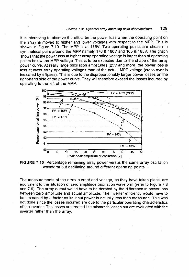
Univers
ity of
Cap
e Tow
n
Section 7.3: Dynamic array operating point characteristics 129
It is interesting to observe the effect on the power loss when the operating point on the array is moved to higher and lower voltages with respect to the MPP. This is shown in Figure 7 .1 o. The MPP is at 175V. Two operating points are chosen in symmetrical pairs ~round the MPP namely 170 & 180V and 165 & 185V. The graph shows that the power loss at higher array operating voltage is larger than at operating points below the MPP voltage. This is to be expected due to the shape of the array power curve. At really large oscillation amplitudes (25V and more) the power loss is less at lower array operating voltages than at the actual MPP voltage (cross-over is indicated by ellipses). This is due to the disproportionably larger power losses on the right-hand side of the power curve. They will therefore exceed the losses incurred by operating to the left of the MPP.
~ ... Q)
~ O> c: ·2 "(ij E Q) ... Q) O> as c Q) 0 ... Q)
Q.
100
99
98
97
96
95
94
93
92
91
90 0 5
FV = 175V (MPP)
FV = 180V
FV = 185V
10 15 20 25 30 35 40 45 50 Peak-peak amplitude of oscillation [V]
FIGURE 7.10 Percentage remaining array power versus the same array oscillation waveform but oscillating around different operating points
The measurements of the array current and voltage, as they have taken place, are ·equivalent to the situation of zero amplitude oscillation waveform (refer to Figure 7.8 and 7.9). The array output would have to be derated by the difference in power loss between zero amplitude and actual amplitude. The inverter efficiency would have to be increased by a factor as its input power is actually less than measured. This was not done since the losses incurred are due to the particular operating characteristics of the inverter. The losses are treated like mismatch losses but are evaluated with the inverter rather than the array.

Univers
ity of
Cap
e Tow
n
130 Chapter Seven: Salvo system performance analysis
7 .3.3 PV\fM envelope
The PWM output voltage of the inverter will be characterised with the same oscillation voltage as on the array voltage. This means that the pulse height which is equiV
1
alent to the magnitude of the array voltage will vary in the same manner as the ~rray voltage. However, the time base of the array oscillation and the inverter switching
. frequency are very different.
250
200
150
100
~ 50
,. ... ~ .... , Q)
0 O> as .:t:::: 0 -50 >
-100
-150
-200
-250 0.0 0.2 0.4 0.6 0.8 1.0
Time (sec)
FIGURE 7.11 PWM envelope curve of the Solvo inverter
This can bet seen in Figure 7.11 where the array voltage oscillation is superimpbsed on the enve~lope curve of the PWM voltage (one line in the graph contains the PWM pulses for half a period - they are merged due to lack of resolution for this time-base).
7 .3.4 Eff1ects of increased input capacitance
The input capacitance was increased from 1100 to 2420 µF. This has the eff~ct of damping the system by presenting the inverter with a more stable voltage supply J The previous tests were then repeated at the same conditions. Only one shape of oscillation waveform was observed. Graph (a) shows two oscillation waveforms operating across different sized capacitors and graph (b) shows the calculated array losses due to the particular range of amplitudes that each waveform occurs in.
The oscillation peak-to-peak amplitude is reduced from around 25V and 1 SV to 1 OV as can be seen in Figure 7.12. The frequency of the osqillation has decreased;.
'
The power extraction from the array improves from 98.7% ± 0.3% to 99.6% ± 0.2% at MPP as shown in Figure 7.12. This also has the effect of decreasing the envelope voltage on the PWM signal but that data is only available for the ML T system (Figure 8.11 and 8.14).

Univers
ity of
Cap
e Tow
n
25
20
15
~ 10 G> Cl 5 as = §; 0
-5
-10
DC capacitance: 2420microF
Section 7.3: Dynamic array operating point characteristics 131
DC capacitance: 1100 microF
95 MPP = 175V Fixed voltage = 175V
94+--r----T---r-"""T"""--.---..----....----t 0.4 0.8 1.2 1.6 2.0 0 5 10 15 20 25 30 35
Time [sec) Peak-peak amplitude of oscillation M
(a) (b)
FIGURE 7.12 Effects of larger DC input capacitance: (a) array oscillation waveforms; (b) percentage remaining array power
7 .4 Voltage to hertz relation
As pointed out in chapter five a considerable amount of difficulty was experienced with the rms voltage measurement. Nevertheless, a few points can be discussed without proper knowledge of the signal and some points can be discussed in comparison.
120r,::::======:;:------:--------, 120 .
[ Log relation )
7ii 1 ooF=====.::::__--:---~"&'==?i..:::::::::_-1 E 2::.
[ Linear relation )
'iii 100+----------~1"7'"----1 E programmed
G> 80-r-------.-----!7'r:;...___;_...c_ __ --l g> = g 60+---__,._,.,::...,_,..-=--------1 G>
~ 40+-->=>'=-=-------------1 .9 G>
3 20r-;i15:6------;:=========::::::::i ( Major gears: 5 to 15 )
0¥---.--..--.--~_;:==;:::=::::;::::::::;;::::=~ 0 10 20 30 40 50 60 70 80 90
Frequency [Hz]
(a)
~ amplitude G> 80+----~~~---:?"'!--7-:----;
E \\ g 60 G>
~ 40+----.,~,..,...-------,-----l
G> 3 20t"°""~r-------::::========~ [Major gears: 5 to 15)
10 20 30 40 50 60 70 80 90 Frequency [Hz]
(b)
FIGURE 7.13 Programmed voltage to hertz relation: (a) logarithmic relation; (b) linear relation
40

Univers
ity of
Cap
e Tow
n
132 Chapter Seven: Solvo system performance analysis
A lot of care was taken to find a suitable and well performing Voltage to Hertz (V/Hz) relation. The voltage boost at low frequency was selected by trial and error and the general V/Hz relation was based on two approaches. One approach is the linear relation which was taken from textbooks and is quite a standard approach, referred to as sub-synchronous V/Hz relation, or here as the linear V/Hz relation. The other approach was taken from the dissertation of Davies (1992). Davies found the parameters of the motor under test and derived an equation to approximately minimise the losses of the motor over the complete operating range. The result was a V/Hz relation where the voltage was proportional to the square-root of the frequency. This is referred to as the logarithmic relation. The voltage amplitudes that were programmE~d are shown in Figure 7 .13.
As can be seen from the graphs the program runs through 1 O major gears. It receives a new amplitude for each major gear and uses that amplitude for all sixteen frequency steps within each major gear. The resolution in terms of voltage amplitudes is therefore low and consequently undermines the effort of deriving an optimum V/Hz relation.
The frequency range of both. programs is 6Hz to 85Hz. The advantage of that is the ability to choose a smaller motor pulley resulting in lower torque requirements from the motor under the same load conditions. In addition the system will be able to run over longer periods of the day. The program cannot overmodulate which is not essential here as sufficient voltage is available from the array.
The array voltage oscillations, as discussed previously, are projected directly on the PWM voltage at the output of the inverter and can be found through the envelope curve of the PWM signal (see Figure 7.11 ). The PWM voltage will have amplitude variations in the range of 1 SV to 30V around 1 BOV (see oscillation voltage in Figure 7.7) resulting in rms voltage variations of 4.2% (7.5V/180V) to 8.4% (15V/180V).

Univers
ity of
Cap
e Tow
n
. Section 7.5: Observed control algorithm characteristics 133
7 .5 Observed control algorithm characteristics
A number of observations have been made on the performance of the control algorithm and especially on situations where the algorithm does not perform as expected. The observations will be described here. Proposals to_wards overcoming some of the control algorithm problems are made in chapter nine.
Basic control algoritlim implementation
The array voltage oscillations as were discussed in section 7.3 are the result of a too simplistic control algorithm that does not take account of the settling time of the system. A thorough description and proposed solutions are given in section 9.1 as both inverters have the same problem.
Stuck motor drive
During normal, continuous operation, the system responds to variations in irradiance levels as expected. When the irradiance drops to a particularly low level (due to a thick cloud for example) it causes the motor to stop running which is as expected. The inverter still receives sufficient power to operate its control electronics (that is it has not reset). As the irradiance level increases again the motor fails to start up. Measurements have shown that power is being used and it was very audible that the inverter was attempting to drive the motor. During this process the inverter loses its array operating point and drops from 180V to 80V. As the power from the array increases again the array voltage moves back to 180V and the rms line current is in the region of 7 A where usually it is in the region of 3.5A to 4.5A.
A similar phenomenon takes place when the motor is stopped through an external force (for example braking the pulley of the discharge head assembly with a shoe) while about 350W of power is available from the. array. The inverter loses its operating point (it has to) and sits at about aov for 3sec and then goes back to 180V. The motor does not start though. It is as if the inverter is in the wrong gear. Both these phenomena can ultimately lead to the burn-out of the power module.
Tests where the pump was deliberately blocked were conducted. This can ultimately be a realistic situation (pump dry-running can result in break-away torque requirements from the pump which the motor might not be able to generate). It was observed that the array voltage remains at 180V (array current during the test was about 2A), that the line current was about 7 A and that the output frequency to the motor was about 9Hz (major gear five). The power module burned-out after 90sec.
Non-essential states of operation
The system goes through _a few modes during start-up and stopping procedures. The modes are confined to periods from the time when the· inverter starts operation (that is, it receives enough power for the controller to operate) to the time when the system is running smoothly. The modes can be divided into four categories: The first mode

Univers
ity of
Cap
e Tow
n
1 34 Chapter Seven: Solvo system performance analysis
is the heating-mode, the second mode is the jerking-mode, the third mode is the sinemode and the last mode is the running-mode.
• In the heating-mode the motor is at standstill, the irradiance is below 220W/m2,
the array operating voltage is between 60V to 1 OOV (as opposed to 1 SOV) and the inverter is delivering current to the motor. It sounds as if the current is pulsed at a rate of 1.5Hz. It can be assumed that the inverter is attempting to drive the motor in its first gear of operation which is major gear number five (in the assembler program).
• In jerking-mode the motor is jerked in regular intervals. The no-operation intervals between the jerks become shorter in time as the input power incmases. This mode prevails from irradiance levels of about 220W/m2 to about 330W/m2
• The steady state array operating point is maintained reasonably well as can be seen in Figure 7 .6. The inverter is still in major gear number five.
• In sine-mode the motor now moves continuously but the speed seems to be varying sinusoidally. This mode occurs at irradiance levels of about 330W/m2
to 3BOW/m2. The program is either in major gear five or six. The pump does not
deliver any water yet.
• In running-mode the motor runs smoothly and delivers water as soon as it enters this mode.
The non-essential modes are therefore the heating and the jerking-mode. They cause unnecessary wear for the motor. The sine-mode can be tolerated but is also not essential since no water is delivered.
Missing pliase
It occurred once that one phase had a bad connection. Unfortunately it was the phase where the measurements were taking place. Therefore nothing can be said about the line current. The motor did continue operation but the question is: Will the inverter experience a break-down due to operation on only two phases. It can be assumed that the line current will exceed the normal values and that the inverter will find it difficult to get the motor started meaning it might operate in low major gears for quite a while. For proper precautions this may have to be investigated again. On the other hand people may be of the opinion that a missing phase is an improbable event.

Univers
ity of
Cap
e Tow
n
Section 7.6: General observations 135
7 .6 General observations
Dynamic conditions
An appropriate test to evaluate the dynamic capabilities of a system is to apply a stepup or a step-down to the input. That was achieved by covering two of the 12 modules in series and then uncovering the modules. This simulates a voltage step but due to the IV characteristics this also translates into a current step. This method poses a disturbance to the system (similar to a thick cloud) which the controller has to correct with an adequate response time. The result is shown in Figure 7.14.
2.5
~ 2.0 'E
200 voltag C'
180 G CD
~ l!! :; 1.5 curren 160 1i 0 >
>-~ :::: 1.0 140 ~ <( <(
0.5 120
0·0 o+---1+-o--20+---301---401---501----+60100
Time [sec]
(a)
2,5,__...._,
~ 2.0 'E ~ ::i 1.5 0
~ :::: 1.0 <(
0.5
10 20
800
30 Time [sec]
(b)
E' g
current 600 'i ~
400 Ill 0. E ::i
200 ~
0.0+0--+---+---+---+----1---+
600
10 20 30 40 50 Time [sec]
(c)
array current .
40 50 so0
FIGURE 7.14 Salvo system response under dynamic conditions: (a) Array voltage and current; (b) array current, phase current, line voltage and torque; (c) array ---..._
current and speed
Graph (a) shows the array current and the array voltage versus time. As the modules are covered the array voltage drops by 1 SV from 185V and after 1 O sec settled back to its fixed voltage point. On uncovering the modules the array voltage rises sharply to 21 OV and drops back to 185V within Ssec. Due to this behaviour the array current does not drop and rise as fast as in the Miltek converter (there is an inherent delay

Univers
ity of
Cap
e Tow
n
136 Chapter Seven: Salvo system performance analysis
due to the sampling of the array voltage). This is an advantage rather than a disadvantage since the inverter is protecting itself indirectly.
Graph (b) shows the array current, the line-to-line voltage, the inverter phase current and the torque. Torque drops rapidly during a moment of 'free-wheeling' and then rises to the new torque requirements. So does the inverter current. On step-up the torque overshoots and then settles to its new value. The inverter current does not follow that trend which makes sense since the array voltage in that moment is quite high (21 OV) resulting in a high line-to-line voltage.
Graph (c) shows the array current with the pump speed. It takes the pump speed about 1 O sec to settle to its new value.
System start-up
The system starts smooth operation between irradiance levels of 380W/m2 to · 400W/m 2
. The power out of the array is 181 Vx0.85A = 154W. Prior to this, the inverter manages to overcome the starting torque at lower irradiance levels, with the help of its DC capacitors as described in section 7.5, but fails to operate smoothly and simply keeps jerking the motor.
The array voltage was sampled under conditions where the motor does not perform a start-up and under conditions where the motor does perform a start-up (Figure 7 .15). Graph (a) shows the array voltage when the motor does not run, where the irradiance level is below 380W/m2
. Graph (b) shows the condition where the motor operates smoothly, at irradiance levels in excess of 400W/m2
.
240
210
240
210 l ·- . .......,.
~ 180
Q) 150 ~
I \
l I \J\ ~\J
Ill I • J"' \11 ~ 180
Q) 150 ~
~·· ··::~··
15 120 > ~ 90
< 60
30
0 0 2 3 4 5 6 7 8 9 10
Time [sec]
(a)
15 120 > ~ 90 .... < 60
30
0o 2 4 6 8 10 12 14 16 18 20
Time [sec]
(b)
FIGURE 7.15 Array ·voltage at start-up: (a) Start failure; (b) start success
Graph (a) shows how the array voltage collapses to 150V, meaning the inverter is drawing too much current and therefore slipped over the knee of the IV curve. Since the motor failed to start the array voltage swings back to nearly open circuit voltage and then it seems as if the inverter tries to start the motor during each oscillation.
-
I • I I
I

Univers
ity of
Cap
e Tow
n
Section 7. 6: General observations 1 3 7
Graph (b) shows how the array voltage drops to about 195V, then increases a bit and then slowly drops to its set operating point of about 178V (in this case). The normal array voltage oscillations can be observed. The difference between these two graphs is that sufficient current is available from the array at the prevailing conditions during the sampling of graph (b).
Inverter tuning difficulties
Tuning requires a measurement device that takes the average of the array voltage (due to the array voltage oscillation) such that the fixed voltage can be set to the desired value. An ordinary digital multimeter is not sufficient as the average needs to be taken over a period of a few seconds. A multimeter with an averaging feature or a low-pass filter with a long time constant are required to tune the array operating point.
PWM switcliing sclieme
This inverter uses a particular method to generate its PWM voltage at different frequencies. The variables that are changeable are the switching frequency (f 6 ) and the number of equal-width pulses that can be repeated within one fundamental cycle. What is of interest is how the repetition of equal-width pulses will affect the frequency spectrum of the output voltage. A general PWM scheme (not overmodulated, synchronous, refer to subsection 2.6.2) has in the worst case (m 1 is even) its first harmonic at the switching frequency with additional sidebands, its next harmonics only as sidebands of twice the switching frequency, its next harmonics at three times the switching frequency with additional sidebands and so on (use Figure 2.5 as a reference but note that conditions are different). Using repetitive equal-width pulses will introduce harmonics at 3 f s• 5 f s• 7 f s and so on that are larger in amplitude than the harmonics occurring in a general PWM schemes. This type of harmonic spectrum certainly degrades motor efficiency but the impact cannot be a assessed here. Therefore the advantage of a high switching frequency drive are compromised to some degree.
Torque pulsations
Torque pulsations were briefly discussed in chapter two (subsection 2.6.4), in the context of harmonic frequencies occurring in the current waveform. However in the Solve and ML T systems, lower frequency torque pulsations were physically observed. Measurements conducted to establish the frequency and magnitude of these torque pulsations did not provide data that could be interpreted usefully, so attempts were made to count the pulses manually. Repeated tests led to the conclusion that the pulsations had a frequency of about 4Hz (20 pulses in 5sec). If the pulsations have the frequency of the array voltage oscillations (which could be expected) then this result comes close to the 3.5Hz oscillation. The faster oscillation recorded in array voltages would not be as detectable (higher frequency and smaller amplitude) as the slower oscillation voltage. There is further discussion on torque pulsations in section 9. 1 .

Univers
ity of
Cap
e Tow
n
138 Chapter Seven: Solvo system performance analysis
7 .7 System performance
The aim of this section is to present the data of the Salvo PVP system and subsystem instantaneously and on a daily basis for different amounts of daily solar irradiation. The daily energy efficiency of the components, the subset (controller and motor), the subsystem and the system and the volume flow are presented for standard solar days from 2kWh/m2/day to 8kWh/m2/day. The emphasis in this subsection is on the shape and trends of the graphs. The performance values are also briefly discussed but further discussion takes place in the comparative chapter ten.
In addition, a solar irradiance profile for a single-axis tracking array has been generated, based on the solar irradiance profile in Figure 6.10. It is referred to as a tracking solar day. System performance predictions for a standard solar day and a tracking solar day are compared.
7 .7.1 Instantaneous performance
The graphs in Figure 7 .16 show the system and subsystem efficiencies and the flowrate as a function of irradiance and array power respectively.
The system efficiency reaches a maximum value of 3.9% from 700W/m2. Above
700W/m2 the flowrate follows a nearly straight line reaching a maximum value of 850l/h just below 1 OOOW/m2
. The subsystem efficiency reaches a value of 33% from 350W array power onwards. This curve shows to some extent the characteristic unevenness that is transferred from the non-linear pump load curve.
5.01..-----·-------~
45 System
· efficiency
1000 flowrate
1000
'* 4.0f---~·--=~~;:::=e;~~~ ;:: 3.5+-----l~'------"7"'-"'-----;
800
'.C
50
45
~ 40
~ 35 c
h ,,_A
./ 800
~
0 ; 3.0·+------Jil''----::::::-~.,.------+
~ 2.5+----'1'--·-r:---------1 G> E 2.0 ~ 1.5+----1----------i
~ 1.0+----1--4------------+ 0.5+----+-,,__ _________ -i
600
400
200
;:. G> iii
~ u::
-~ 30
ii 25
f6 20
~ 15 -8 :J 10
Cf) 5
0
,,,...-. --" ~- -
~ ,,,,k" "subsystem
i ·' ,,r' efficiency
rf x·-' // // 200
II 0·&,o 400 500 600 700 800 900
Plane of array irradiance [W/sqm)
0 1000 100 200 300 400 500
0 600
Array power [W]
(a) (b)
FIGURE: 7.16 (a) Solvo system performance and (b) subsystem performance
The uncertainty in the system efficiency data is:
LJabs (l\ys )1050W/sqm = 12.1 % LJrel (nsys )10SOW/sqm = 6.9% uabs (nsys hsowtsqm = 15. 7% U rel ( nsys hsowtsqm = 9 .4 %
.. I
I

Univers
ity of
Cap
e Tow
n
Section 7. 7: System performance 139
The uncertainty in the subsystem efficiency data is:
u (ri ) = 6.3% abs subsys SOOW
U 1 (r-. b )soow = 2.5% re · 'Su sys
U (r-. }3sow = 6.5% abs · 'Subsys
u (r-. ) = 2.9% rel · 'Subsys 350W
The uncertainty in the flowrate data is:
uabs (0)200-+ 10001/h = 6.1 % Ure1 (Ohoo ..... 10001/h = 2.2%
The subsystem efficiency presents itself as the data with the lowest uncertainty and therefore the most reliable for comparison to other systems (absolute uncertainty in the region of 6.4%). The largest uncertainty is introduced through the flowrate calibration. The relative uncertainty at full input power is 2.5% and increases minimally as the input power decreases. Subsystem efficiency data can therefore be used with good reliability for comparison among the three PVP systems. The absolute uncertainty in the system efficiency is high as a result of the pyranometer errors. The relative uncertainty remains relatively high as the spectral response error in the pyranometer cannot be assessed.
7.7.2 Daily energy efficiency performance
The daily energy efficiency (DEE) is calculated by dividing the total energy out of a componenUsystem by the total energy into a componenUsystem over the course of a standard solar day. Therefore the DEE's of components are partly dependent on surrounding component performances and matching. For example, the inverter DEE depends on the performance of the array: poor array performance will result in a poor DEE of the inverter. The method for daily energy efficiency calculations is presented in appendix A5.
The DEE of the components, subset and subsystem is shown in Figure 7.17. The inverter DEE increases from 15% to 78% ending with a small gradient towards a SSD of 8kWh/m2/day. The motor reaches a nearly constant value at 71 %. It shape follows its instantaneous efficiency curve. The pumping set reaches a peak at 55% and does not increase any further beyond a SSD of 7.3kWh/m 2/day.
Both the subset and the subsystem efficiency curves become flatter at higher daily irradiation levels. They reach values of 56% and 31 % respectively at 8kWh/m2/day. Subsystem efficiency is zero at 2.3kWh/m 2/day. Subset efficiency is zero at 2kWh/m2/day.

Univers
ity of
Cap
e Tow
n
140 Chapter Seven: Salvo system performance analysis
~ 1ot----------::::::::=:;;:z~;,_~---:;::;:-i !: 50+----------=:~:;.....;.----i ~ 50,+---~--,?.--7"e,_ _________ -I ~
-~ soJ--~~~.L:;;::....c::::::::::::=::=:=~::::=J i 40+--------_.,...'--------------" ·c::;
iE w 40-1---./-,~'.+----------------_,,_---I
iE subsystem w 30+-----"7''--------------==----~
i;; i;; ~ 301-l---/:-l-----------------------1 c:
~ .
c: 20----------'-------------" w 2:-w 20.j.....,L-t-.'-----------------1 2:-
~ 10.l-i'..J-------------------=======1 "m 10+--+-------------------l Cl
O+"'-..:;;...-.-----.----~----.-----..-----~ 3 4 5 6 7 Standard solar day [kWh/sqm/day]
(a}
2 3 4 5 6 7 Standard solar day [kWh/sqm/day]
(b}
FIGURE 7 .17 Solvo system daily energy efficiency: (a) components and (b) ~ubset and subsystem '
Figure 7.18 di1splays the DEE of the .system and the daily volume flow as a function of the standard solar day. System ope:ration starts beyond 2.3kWh/m2/day. The system efficiency reaches 3.3% at 8kWh/m2/day and the system delivers 5.85m 3 over such·a day.
The comparison between a standard solar day and a tracking solar day (TSD) is shown in Figure 7.19. Displayed are the DEE of the system and the volume flow. The differ,ence between the SSD and the TSO based on the SSD is shown in the adjacent graph.
8

Univers
ity of
Cap
e Tow
n
~ >. 0 c: G>
"<3 :e w >. C> Qj c: w 2:-·a; 0
Section 7. 7: System performance 141
The difference between the DEE of the system at SSD and TSO is about 7% at 11 OOW/m2 noon peak irradiance. The difference increases as the daily peak irradiance decreases and rises to 20% at 600W/m2 and reaches 60% at 350W/m2 where the subsystem ceases to operate for SSD conditions. The shape of the volume flow curve is similar but has a higher percentage difference. At 11 OOW/m2 noon peak irradiance the difference is 35% and reaches a value of 53% at 600W/m2
.
4.5 9 110 ';::"
4.0 ... 8 GI "iii
~ 100 GI E 90
3.5 7 0 /
._ .. ~. c: 0 Cll 80 \ 3.0 I .. 6 :0 E .l-··, - :::> 70 .£. 0
2.5 ······· \ 't: 5 G> 60 Q.
2.0 4 ~ 0 50 G> (/)
1.5 3 E (/) 40 ,, .. ··· :::> ..... 30
1.0 ...
2 0 G> > ~ -- system DEE 2:- 20
0.5 1 ·a; 0 10 --·-··· volume flow 0 (/)
t-0.0 0
no o ration s stem DEE below 350 W/sqm for SSD
300 400 500 600 700 800 900 1000 1100 0 300 400 500 600 700 800 900 1000 1100
Noon peak irradiance [W/sqm) Noon peak irradiance (W/sqm)
(a) (b)
FIGURE 7.19 Tracking solar day and standard solar day for the Solve system DEE and the volume flow: (a) performance and (b) percentage of TSO over SSD
This graph shows that a tracking array becomes more beneficial in comparison to a fixed array at sites where the solar irradiance levels are generally low, like in the region of 600W/m2 to 800W/m 2 (sites with less than 600W/m2 noon peak irradiance should probably not consider PVP's). On the other hand, sites with such low noon peak irradiance levels will have a higher proportion of diffuse irradiation and will therefore not benefit from a tracking array as much as indicated in Figure 7.19 above.
As indicated in chapter six (subsection 6.3.4), the average noon peak irradiance levels for Windhoek never fall below 900W/m2 on a tilted surface with an angle of tilt equal to 20°. ·

Univers
ity of
Cap
e Tow
n
Chapter Eight
ML T SYSTEM PERFORMANCE ANALYSIS
The chapters on the prototype inverters (chapters seven and eight) each stand on their own and can be read independently of one another. Because of this there is a small amount of duplication with the result that some introductory paragraphs are the same or similar.
This chapter presents and discusses the inverter and motor efficiency, the steady state array operating point characteristics for fixed voltage operation (speed sensor disconnected) and maximum speed tracking, the dynamic array operating point characteristics, the voltage to hertz relation, the control algorithm characteristics and general observations on the system. This is followed by the instantaneous system and subsystem performance evaluation and by the daily energy efficiency evaluation of the components and the system.
The derivation of the absolute and relative uncertainty in the acquired data is presented in appendix A3.6. The derivation of the stated uncertainty in the efficiency data is given by an example in appendix A3.7. All uncertainties are stated as a plusminus percentage of a full-scale reading.
System tu11i11g
The system was tuned for two modes of operation, one being fixed voltage operation (FVO) and the other being maximum speed tracking (MST). In both modes of operation the array operating point was adjusted and a suitable pulley size was selected. The MST mode required additional adjustment at the speed potentiometer.
The array voltage was adjusted to a steady state value of about 90V for both operation modes. This was found to be close to the MPP at cell temperatures of 47°C (refer to Figure 6.8).
The choice of motor pulley was guided by two criteria (the pulley of the discharge head assembly remained the same for all tests, being 247PCD):
• the inverter should be able to just reach its maximum programmed output frequency at the maximum irradiance level
• the start-up delay should be minimised
For FVO the pulley choice was between 97PCD (pitch-centre diameter), 112PCD and 11 SPCD. The 97PCD pulley reached its 65Hz output frequency at 1 OOOW/m 2 and did not respond to higher irradiance levels. The 11 SPCD pulley reduced the operating range of the system considerably, that is the system would only start up at high levels

Univers
ity of
Cap
e Tow
n
144 Chapter Eight: ML T system performance analysis
of irradiance (eg. 850W/m2). The 112PCD pulley permitted start-up to occur at about
750W/m2 which is still higher than for the 97PCD pulley. But then the 112PCD pulley managed a higher pump speed (about 40rpm higher on average) over the complete operating range. The 112PCD pulley was consequently chosen for FVO.
For MST the pulley choice was between the 118PCD and the 125PCD pulley. It was not very clear from the sampled data which pulley performed better over the whole operating range as both pulleys managed higher pump speeds at particular irradiance levels. The 118PCD pulley reached a higher maximum speed at the same level of irradiance and would also start up earlier. The 118PCD pulley was therefore chosen.
The speed potentiometer had to be adjusted in MST mode. This was not required to maximise speed but rather to enable the motor to start up at the lowest possible input power level (the tuning difficulties are discussed in subsection 8.6). The case occurred where the motor turned at a constant speed of about 170rpm (Spump = 90rpm, virtually no water is pumped) even though it could potentially turn a tot faster since it was receiving substantially more power than required for start-up.
8.1 Inverter and motor performance
This section deals with the inverter, the motor and the subset efficiency at standard and at higher head as well as the characteristic inverter and motor curves.
8.1.1 Efficiency at standard head (75m)
The efficiencies of the subset components are discussed only briefly for fixed voltage operation but more elaborately for maximum speed tracking.
The inverter efficiency includes the losses due to the dynamic array operating point characteristics (as will be discussed in section 8.3). It does not include the array output losses due to steady state operation away from the MPP. It also does not include the mismatch losses between the inverter and the motor which are caused by the harmonics in the current waveform. These losses are included in the motor efficiency.
The uncertainties in the efficiency results are stated for MST operation but not for FVO. However they are likely to be very similar in magnitude.
Fixed voltage operation
The FVO operating range of the subsystem is quite narrow. Subsystem operation starts at an input power of about 350W. Operation was tested up to 500W. The result is shown in Figure 8.1.
Both components maintain a fairly constant efficiency value. The inverter remains at about 90% and the motor at about 67%. The resulting subset efficiency is 60%.

Univers
ity of
Cap
e Tow
n
100
90
80
70
~ 60
g 50 .g! 0
ffi 40
30
20
10
0
Section 8. 1: Inverter and motor petformance 14 5
inverter - ~
L!r ~
motor A/
-....- ~ ,_ Tf
"""•"" ... ~~
\ subset
combination
0 50 100 150 200 250 300 350 400 450 500 550 Array power [W]
FIGURE 8.1 ML T inverter, GEC motor and subset efficiency versus input power: Fixed voltage operation
Maximum speed tracking
The inverter and the motor efficiency have been recorded from 120W to 51 OW array power. This is displayed in Figure 8.2. The inverter starts with an efficiency of 70% that rises to over 90% at 300W. It remains at about 92% and rises to 94% on the last data point which is at 51 OW (confirmation of this data point was found in three separate data sets).
100
90 inverter = - J'l
-- -
- 91'
80
70
)<:I -=
~ motor
~ 60 ~ 50 c: Q)
·c:; 40 = w 30
~ ........ ~·-·*-·"*··'* ;.~·· '\ .~ ,. r ~ .. ,.~ .....
" .*····~····· subset
rr combination
20
10
,!
J ~~:l
0 0 50 100 150 200 250 300 350 400 450 500 550
Array power [W]
FIGURE 8.2 MLT inverter, GEC motor and subset efficiency versus input power: Maximum speed tracking

Univers
ity of
Cap
e Tow
n
146 Chapter Eight: ML T system performance analysis
The uncertainty in the inverter efficiency data is:
uabs (ninv )soow = 7 .6% Ural (ninv )soow = 4.8% Uabs (ninv hsow = 16. 7% Ural (ninv hsow = 10.7%
The inverter losses, Figure 8.3, are on average between 30W and 40W with a low of 23W between 300W and 350W input power. The losses can be divided into constant and varying losses. The constant losses consist of the power supply losses, microcomputer power requirements and the drive circuit requirements. The power supply losses are likely to be relatively high as a voltage regulator circuit is used. The microcomputer and drive circuit power requirements have been approximated by Davies (1992: 71) to be 200mA at 1 SV which is equivalent to 3W. This power has to be produced from the array operating voltage which is about 90V. The power supply losses are therefore equivalent to 75V x 200mA = 1 SW. The resulting constant losses are consequently 18W but will be taken to be 20W (since the array voltage can also operate at 1 OOV).
c~
~ 0 Q) VI VI .Q ,_ Q) t: ~ .E
50
45
40
35
30
25
20
15
10
5
0 0 50 100 150 200 250 300 350 400 450 500 550
Array power [W]
FIGURE 8.3 ML T inverter losses: Maximum speed tracking mode
The varying losses are the switching losses and the conduction losses. These vary because the line current varies to some degree. In addition to this the switching losses also vary due to changes in the switching frequency. Both can be taken from Davies' dissertation ( 1992) as they are calculated under similar conditions (that is the line current is about 3A and the array voltage is 95V). The switching losses are therefore (Davies 1992: Figure 42) 6.SW at 20Hz, 7 .SW at 35Hz and 3.6W at SO Hz. The inverter changes from sinusoidal PWM to harmonic elimination PWM at 50Hz, hence the drop in switching losses. The conduction losses were calculated for a maximum line current but will usually be less than that. Davies (1992: 70) calculated them to be 1 OW. For a minimum line current of 2.SA (see Figure 8.5 a) this loss evaluates to 2.3W. I

Univers
ity of
Cap
e Tow
n
Section 8. 1: Inverter and motor performance 14 7
Combining all the losses results in 37.5W maximum and 26W minimum. This is in agreement with the inverter losses as they are displayed in Figure 8.3. However, the minimum of the graph, occurring at 31 OW input power, does not logically correspond to the calculated values since the line current is at its maximum (see Figure 8.5) between 300W to 320W (pump torque peaks slightly and inverter voltage drops). This means that the conduction losses and the switching losses will be high. Consequently the inverter efficiency should be low at this point but actually goes through a peak. I am not able to find an explanation for this behaviour unless the drive parameters programmed into the inverter are unsuitable for the motor in this region or it could be possible that the program changes to harmonic elimination at 40Hz instead of 50Hz (the ML T inverter documentation was not up-to-date). It was also possible that the measurement equipment might have experienced some disturbances due to inverter switching frequencies. However it is certain that this inverter efficiency curve was very repeatable (observed in at least five different data sets) and that it was logged under steady state conditions.
The motor efficiency (Figure 8.2) is about 3% for input powers of 120W to 160W (the motor runs at a base speed of 30rpm) and then rises fairly sharply to about 50% where it more or less remains until 330W input power. It then rises to about 67% I 68% until 51 OW input power is reached. It then reaches 70% on the last data point which occurs at 51 OW input power. The motor as tested therefore comes to within 6% of the motor specifications (at 50Hz, 70VLL it is 75.6%). This is acceptable as the motor receives some fre.quency harmonics as can be seen in the distorted line current waveform in Figure 3.9.
The shape of the motor efficiency curve seems to follow the shape of the pump efficiency curve once more than 200W input power is received. Here therefore it could be that the pump load requirements feed through and determine the shape of the motor efficiency curve. The shape and the magnitude are of course also affected by the harmonic content of the current waveform and the time-base at which the switching frequency is changed. The change in PWM switching scheme was expected at about 400W array power (inverter frequency of 50Hz) but at that point there is no discontinuity. Which of these factors determines the shape would have to be tested with a linear load.
The uncertainty in the motor efficiency data is:
uabs (nmot }475w = 8.3% U (n ) - 6.1% rel mot 475W -
uabs (nmot hsow = 14.5% urel (nmot )2sow = 9.8%
The subset efficiency (Figure 8.2) is 3% at input powers of less than 160W. Between 200W and 330W the efficiency is increasing from 40% to 50% and reaches 60% at an input power of 370W. It reaches 66% on the last data point at 51 OW input power. The shape of the curve is very similar to the motor efficiency curve since the inverter efficiency curve is reasonably linear.

Univers
ity of
Cap
e Tow
n
148 Chapter Eight: ML T system performance analysis
The uncertainty in the subset efficiency data is:
uabs (1\ubset )soow = 4.9% urel ("'subset )soow = 4.2% uabs ("'subset hsow = 5.6% urel ("'subset )2sow = 4.9%
The uncertainty in the subset efficiency is lower than the individual inverter or motor efficiency. Due to a partly 'programmable' efficiency of the inverter and therefore indirectly a partly 'programmable' efficiency of the motor it was decided to use the subset performance as the most appropriate gauge for the inverter/motor evaluation (that is the inverter-motor combination has to be optimised not the inverter by itself). From a measurement point of view this is supported due to lower uncertainties in these data sets. The lower uncertainty is mainly due to high-accuracy components of the array current and array voltage data acquisition circuits.
The bumps that generally occur in the graphs of the efficiency curves are due to changes in output voltage and probably due to the unstable torque characteristics of the load. ·
8.1.2 Effftciency at higher head
The tests that were conducted to evaluate the inverter and the motor performance as the static head increases were only partly successful. Unfortunately the power meter was not correctly connected. Nevertheless, the data for the subset can be evaluated.
70
60
~ 50 >- 82m head (.) c: 40 Q)
"(3
!E Q) 30 Q) j UJ .0 ::> 20 en
10
O+----i.----.,.~-..-~-.-~-r-----i.----.,.~-,-~-,-~-r------1
0 50 100 150 200 250 300 350 400 450 500 550 Array power [W]
FIGURE 8.4 ML T subset efficiency at two static heads
Figure 8.4 shows the subset efficiency at two heads which are not that far apart. The efficiency at 75m is slightly better than the efficiency at 82m. The average difference is 2%.

Univers
ity of
Cap
e Tow
n 'E z ~ CD :> O' .... £ ~
c Q) .... :; 0 Q)
"' al .c Cl..
Section 8.1: Inverter and motor performance 149
Should the available input power be increased than the subset efficiency would increase due to an increase in inverter and motor efficiency (constant losses in the inverter reduce relatively and the motor efficiency increases as it gets closer to its design operating conditions).
8.1.3 Characteristic inverter and motor curves
The characteristic inverter and motor curves under the particular load conditions are shown in Figure 8.5. The inverter line current has similar tendencies to the torque curve of the pump (Graph a). Both reach a peak at 300W array power although the change in current is quite marked. This may well be due to invertervoltage variations due to array voltage variations (compare to array voltage in Figure 8.7).
4.0
3.5 ,,....
3.0
I 2.5
{
2.0
1.5
1.0
/~I
torque ..
current
~ .~ "iii ~
"N 6 ~ c: Q) :> O' ~ -.... Q) 1: CD >
.E
90 900 speed ,. ...
80 800 ._, 70 700 ...
)II 60 600
50 500
40 -·-···-- 400 frequency
30 300
20 200
10 100
0 0 100 200 300 400
Array power [W] 500 600 100 200 300 400 500 600
Array power [W]
. (a) (b)
FIGURE 8.5 ML T characteristic subsystem curves: (a) phase current and pump torque; (b) frequency, slip and pump speed
The frequency and the pump speed have the same response curve (graph b). The speed curve exhibits a particular tendency of the ML T system. The motor runs at a base speed of about 30rpm (ie Spump = 15rpm on the graph; speed ratio is about 2) until it reaches a particular power threshold from where it then speeds up to about 400rpm (ie Spump = 200rpm). The slip decreases rapidly once the motor leaves its base speed. A small peak occurs at 300W array power which corresponds to an increase in the phase current (graph b).
'E .§: "O Q) Q) a. I/)
a. E :>
Cl..

Univers
ity of
Cap
e Tow
n
150 Chapter Eight: ML T system performance analysis
8.2 Steady state array operating point characteristics
The ML T inverter has two principal operating modes which are fixed voltage operation (FVO) and maximum speed tracking (MST). Both were tested extensively. It has to be stated clearly though that in retrospect the MST mode of operation was not tested correctly as it was not given sufficient time to seek its maximum speed at each data acquisition point.
Fixed voltage operation
The mean array voltage (5second average) is displayed in Figure 8.6. The voltage remains at about 93V. The maximum deviation found in a data set was 4.5V. Usually it was about 3V maximum.
100 6.0
90 5.5
80 5.0
~ < Q) 70 4.5 ~ C>
~ co ~ 60 4.0 .... 0 :J > 0
~ 50 3.5 ~ .... .... .... <( <(
40 3.0
30 2.5
20 2.0 750 800 850 900 950 1000 1050
Plane of array irradiance [W/sqm]
FIGURE 8.6 Fixed voltage operation of the ML T inverter
Below 750W/m2 the system failed to reach a steady state operating point. The inverter would 'run up' the IV curve of the array from about 120V but would pass through the array voltage set-point and sit at about 35V. Only when the level of irradiance was in excess of 750W/m2 would the system start proper operation.
Maximum speed tracking
I was unable to assess how long it would take the inverter to find its maximum speed operating point and therefore indirectly move towards the MPP. It was thought that the hunting for the maximum speed would be accomplished within a good 30 seconds. It became clear from the data though that this was not the case. The implications are twofold: One, the performance of the MST program cannot be evaluated properly here due to poor test procedure as the system requires a few minutes to track the maximum speed and two, the possibility that MST algorithm cannot be properly implemented under the conditions of array voltage oscillations described in section 8.3.

Univers
ity of
Cap
e Tow
n
Section 8.2: Steady state array operating point characteristics 151
The latter point will be argued for in subsection 8.5.3. The data is nevertheless shown in Figure 8. 7.
100
90
80
~ 70 Q)
g> ~ 60 0 > ~ ... 50 ... c(
40
30
20 300
Average module temperature: 39 degC, deviation: +/- 3degC
voltage, as irradiance increases
400 500 600 700 800 900 1000 1100 Plane of array irradiance [W/sqm]
FIGURE 8.7 ML T inverter-control of the array operating point while in maximum speed tracking mode
The array voltage is displayed for increasing and decreasing irradiance (the system received a settling time of 25sec for each data point). It was originally thought that the inverter exhibited hysteresis. That is why the module temperature is specified. The inverter traces out two paths for increasing and decreasing irradiance (consistent for .three data sets). While the irradiance level increases the voltage is generally higher as opposed to when the irradiance level decreases. This behaviour gives the
. impression that the MST program drives its reference voltage window to the top limit as the irradiance increases and to the bottom limit as the irradiance decreases. The impact of the speed tracking algorithm thus has quite a substantial impact on the fixed voltage tracking algorithm. This should not be the case since the program takes one speed sample for every twenty-five voltage samples and therefore indicates that the MST program is not operating as it should or is prevented from doing so (further discussion in subsection 8.5.3).
The MST evaluation would have included calculating the MPP co-ordinates (current and voltage) from the collected array data based on the plane of array irradiance and the module temperature that prevailed when the ML T system was tested. This would have been compared to the operating point co-ordinates that the ML T inverter traced out on the IV curve of the array.

Univers
ity of
Cap
e Tow
n
152 Chapter Eight: ML T system performance analysis
8.3 Dynamic array operating point characteristics
The mean array voltage proved to remain quite close to the set-point to which it was tuned (FVO only). The instantaneous voltage though has quite a large movement about that mean value. As this could result in a diminished array output and can have a negative impact on the motor the effect of this array voltage oscillation is analysed here.
It is common for switch-mode inverters to have a ripple voltage on the DC-side input which is due to the switching scheme employed by the inverter. The magnitude of the ripple is dependent on the switching frequency of the inverter (inversely related). Its frequency is the same as the switching frequency. The ripple discussed here (referred to as an oscillation voltage) is the result of the type of control algorithm implemented in the inverter (a detailed analysis of the control algorithm is in section 9.1 ). This section purely evaluates the impact of the oscillation voltage on the array performance and on the shape of the PWM inverter output signal. The effect of a larger input capacitance on the array voltage oscillation is also evaluated.
8.3.1 Shapes of oscillation waveforms
The typical shapes of oscillation waveforms that were encountered are displayed in Figure 8.8.
25 25
20 20
15 15
~ 10 ~ 10 G> Cl 5 co = g 0
G> Cl 5 co = 0 0 >
-5 -5
-10 -10
-15 0.2 0.6 1.0 1.4 1.8
-15 0.5 1.0 1.5 2.0 2.5 3.0 ~1.5
Time (sec] Time (sec]
(a) (b)
FIGURE 8.8 Typical array voltage oscillation waveforms riding on 90Varr
They have different amplitude and different shapes. The superimposed. ripple is caused by the switching of the inverter. The frequency of the oscillation voltage in graph (a) is 3.4Hz with a peak-to-peak amplitude of about 16V. The oscillation voltage in graph (b) has a frequency of 1.7Hz but that is not really obvious. The peak-to-peak amplitude of the signal is about 30V. The period between the large positive amplitude spikes is in the range of 1.1 sec to 1.3sec. Shorter and longer periods have also been observed namely 800msec to 1.7sec.

Univers
ity of
Cap
e Tow
n
Section 8.3: Dynamic a"ay operating point characteristics 153
At what fundamental inverter frequencies both oscillation waveforms occur is not known. However the shape and magnitude do not vary considerably at different levels of input power.
8.3.2 Array power losses
In order to assess the impact of the oscillation waveform on the array output, the two waveforms from above were superimposed on the steady state array operating point by providing information of a characteristic array power curve. The method is described in appendix A6.
The result of this procedure is shown in Figure 8.9. The two lines represent the actual oscillation waveforms. The amplitude of the waveform is scaled to simulate waveforms of smaller and larger amplitude. Waveform 1 represents graph (a) in Figure 8.8 and waveform 2 graph (a). Over the whole peak-to-peak amplitude range waveform 1 has larger array losses than waveform 2. Therefore the integral of oscillation waveform 1 is larger than the integral of waveform 2.
100 Waveform2
[ 99
.... 98
~ Waveform 1 97 a.
C> 96 c: ·2 ·ca 95 E ~ 94
...............
Q) C>
93 as c Q)
92 e Q) MPP = 91V Q.. 91
Fixed voltage = 91V
The most common amplitu es encountere
90-1-~~...-~--.~~---.-~~--r-~~-r-~~-.-~--t
0 5 10 15 20 25 30 35 Peak-peak amplitude of oscillation [V]
FIGURE 8.9 Percentage of remai~ing array power versus a range of oscillation waveform amplitudes while operating (on average) at MPP
The oscillation waveform operates around the MPP at 91V. Therefore the array losses are zero at zero peak-to-peak oscillation amplitude. The window indicates the amplitude range that was encountered resulting in array output losses of 1.5% to 4%.
Figure 8.1 O shows the effect of operation away from the MPP. The array output losses due to operating 4V above the MPP are shown at zero peak-to-peak amplitude. They are about 1.3%. Due to the shape of the array power curve the losses due to the oscillation waveform are not equivalent to their losses at MPP plus the offset (that is 1.3%). For example, the losses at 25VPP are 6% at an operating voltage of 95V and 3.8% at MPP (3.8% + 1.3% < 6%).

Univers
ity of
Cap
e Tow
n
1 54 Ct1apter Eight: ML T system performance analysis
100 MPP = 91V Waveform2
~ Fixed voltage = 95V
~ 98 ....
[ 96
C> c: ·c: ·a; E ~ Q)
92
' The difference to 100% is Q) due to steady state operation e 90 Q) away romt e D.
88 0 5 10 15 20 25 30 35
Peak-peak amplitude of oscillation [V]
FIG URIE 8.1 O Percentage of remaining array power versus a range of array voltage oscillation amplitudes while operating (on average) 4V to the right of MPP
The impact of an oscillation waveform increases as the operating voltage increases beyond thE~ MPP voltage and the impact decreases as the array voltage becomes lower than the MPP voltage (see Figure 7.10).
The array current and array voltage measurements, as they have taken place, are equivalent to conditions of zero oscillation amplitude. The array output would have to be derated by the difference in power loss between zero amplitude and actual amplitude. The inverter efficiency would have to be increased by a factor as its input power is actually less than measured. This was not done since the losses are incurred due to the particular operating characteristics of ·the inverter. These losses are therefore treated as mismatch losses but are put on the inverter's account.
8.3.3 PWM envelope
Since the inverter uses a switch-mode scheme to drive its output the array voltage oscillations will be transferred to its output voltage. This can be seen on the .PWM envelope curve shown in Figure 8.11.
The time-base for the oscillation waveform is usually longer (about 3.5Hz) than the fundamental frequency of the output signal (3Hz to 65Hz). For example, at 50Hz fundamental frequency the output voltage will go through 14 cycles as the oscillation waveform goes through one cycle.
• ...

Univers
ity of
Cap
e Tow
n
Section 8.3: Dynamic a"ay operating point characteristics 155
150
125
~ 100
Q) 75 g> 50 .::: 0 > Q)
.E 6 -.
Cl> :§ ::? 3: a..
25
0
-25
-50
-75
-100
-125
-150 0.0 0.2 0.4 0.6 0.8 1.0 1.2 1.4 1.6 1.8
Time [sec)
FIGURE 8.11 PWM envelope curve of the ML T inverter
8.3.4 Effects of increased input capacitance
The input capacitance was increased from 2040µF to 67 40µF to observe the impact on the array voltage oscillations. It essentially dampens the system by providing a stiffer voltage supply.
25~-------------------~
20
15
10
DC capacitance: 6740 microF
DC capacitance:
2040 microF ~
5
0+.+--1111;-1+-'t-+.-fl~--\--+--f-..,..+-lf'-f---t+-t-t--:t;---t+---t~
-5
-10
-15
-20+--~--.----.----.----.---.--_,.--_,.--~--t 0.0 0.2 0.4 0.6 . 0.8 1.0 1.2 1.4 1.6 1.8 2.0
Time (sec]
FIGURE 8.12 Effects of a larger DC input capacitance on the oscillation waveform
The oscillation voltage decreased to 1 OV PP in amplitude while the frequency hardly changed (3.2Hz). Figure 8.12 shows the graph.

Univers
ity of
Cap
e Tow
n
156 Chapter Eight: ML T system performance analysis
Array power losses I
Figure 8.13 shows that the array output losses have been reduced from the 1.5% to 4% range to the 1 % to 3% range. This is not a lot considering that the input capacitance was increased by a factor of 3.3.
[ ... ~ a. C> c: ·2 "(ij E ~ Q) C> as c: Q)
e Q) c..
100
99
98
97
96
95
94
93
92 0
~ 6740uF DC capacitance:
..... , 2040uF
""'-- i"-.... " r"--~
""',,~ ''t
""" ~ MPP = 91V ~ Fixed voltage = 91V
5 10 15 20 25 30 ·Peak-peak amplitude of oscillation [V]
FIGURE 8.13 Percentage remaining array power with larger DC input capacitance .I
The oscillation waveform shape as in Figure 8.8b was not sampled again f6r the increased capacitance condition. It does however still occur as will be shown. 81:.1t this is the reason why the window for the increased capacitance still stretches down to 3%.
PWM envelope
The change in the envelope curve, Figure 8.14, is interesting in that most of the oscillations have been reduced considerably (compare to Figure 8.11) except for an oscillation occurring every 1.2sec (at the arrows). The same oscillation can be observed in Figure 8.11 (arrows) and it probably has the same shape as seen in the graph in Figure 8.8b but with a reduced oscillation voltage between the peaks.
This phenomenon is most likely due to another form of oscillation. I have found no reasdnablH explanation for its source.
I
I
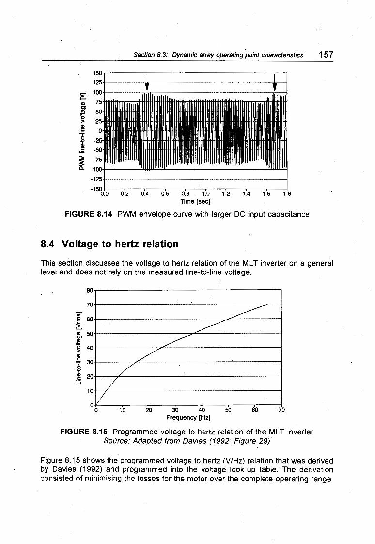
Univers
ity of
Cap
e Tow
n
Section 8.3: Dynamic a"ay operating point characteristics 157
150
125
~ 100
Q) 75 C> C'IS 50 ~ 0
25 > Q) c: 0 6 -25 '";' Q)
~ -50 ::!: -75 ;: D.. -100
-125
-150 0.0 0.2 0.4 0.6 0.8 1.0 1.2 1.4 1.6 1.8
Time [sec)
FIGURE 8.14 PWM envelope curve with larger DC input capacitance
8.4 Voltage to hertz relation
This section discusses the voltage to hertz relation of the ML T inverter on a general level and does not rely on the measured line-to-line voltage.
80
70
Ci) E 60 .... ~ Q) 50 C> Jg 0 40 > Q)
.5 30 I 0 -I Q) 20 c: :::i
10
10 20 30 40 50 60 70 Frequency [Hz]
FIGURE 8.15 Programmed voltage to hertz relation of the ML T inverter Source: Adapted from Davies (1992: Figure 29)
Figure 8.15 shows the programmed voltage to hertz (V/Hz) relation that was derived by Davies (1992) and programmed into the voltage look-up table. The derivation consisted of minimising the losses for the motor over the complete operating range.

Univers
ity of
Cap
e Tow
n
158 Chapter Eight: ML T system perfonnance analysis
The line-to-line voltage in the low frequency range will be boosted and will not run down to zero volts. The V/Hz curve will not be implemented continuously but is approximated by nineteen amplitudes. The best case would be 3.26Hz per amplitude division which would result in 19 amplitude steps spread evenly over 3Hz to 65Hz. I cannot find any reference as to whether this is the case. In my opinion the hardware offers the flexibility to assign amplitudes in these frequency ranges.
The array voltage oscillations, as discussed in the previous section, result in equal variations of the PWM voltage. Consequently, the PWM voltage will vary by 7.9% to 13.2% (15VP/2/95V and 25VP/2/95V respectively). That is extremely high and undermines the careful derivation for an optimum V/Hz as performed by Davies.
The benefits of generating the PWM signals directly out of the microcontroller are realised in its ability to generate an overmodulated PWM signal. Through these means a larger line-to-line voltage can be generated than in an inverter with a maximum modulation index of one. A modulation index of one would result in a maximum rms voltage of 0.612 x Varr which gives 58Vrms for 95V array voltage (Mohan et al. 1989: 132). With overmodulation a rms voltage of 7 4.1 V can be generated from 95V. However that voltage would have degenerated into a squarewave resulting in undesirable low frequency harmonics. This inverter utilises overmodulation in combination with harmonic elimination and therefore can generate a higher rms voltage while eliminating the 5th, ]1h, 11th and 13th harmonics.
8.5 Observed control algorithm characteristics
A number of observations have been made regarding the performance of the control algorithm. Both FVO and MST implementations have some characteristics which may be undesirable or non-essential. These are discussed below.
8.5.1 Basic control algorithm implementation
The array voltage oscillations as discussed in section 8.3 are the result of a too simplistic control algorithm that does not take account of the settling time of the system. A thorough description and suggestions are given in section 9.1 as both inverters have the same problem.
8.5.2 Fixed voltage operation
Narrow operating range
The operating range of the inverter is too narrow with the FVO program installed, as can be seen in Figure 8.17 in section 8. 7. At irradiance levels of less than 750W/m2
(but larger than 540W/m2) the subsystem performs a start-up but passes through its
operating point on the array IV curve and settles at an array voltage of 35V. The motor stalls and a restart may take place. In MST operation the subsystem is able to run at much lower input power levels. ·
I I
I

Univers
ity of
Cap
e Tow
n
Section 8.5: Observed control algorithm characteristics 159
FVO but not entirely FVO
It was found that the FVO program does not use the array voltage as its only control variable for its decision making. The microcontroller has a reset circuit that requires a square-wave at its input in order not to reset the microcontroller. This is provided from one of the PWM signals when running in fixed voltage mode (FVO). The inverter responds differently though when the speed sensor is connected to this reset circuit (called the watchdog circuit) which also feeds into the speed-sensing circuit. This is very obvious since the inverter is then able to operate at much lower input powers, very similar to the MST program.
Therefore, firstly, the FVO program uses the speed signal for control purposes (other than reset) but should use the array voltage as its only decision parameter. Secondly, it is possible that the PWM signal at the input to the watchdog and speed sensing circuit may affect the performance of the FVO program negatively (for instance the narrow operating range).
Non-essential states of operation
During FVO operation and feeding a PWM signal to the watchdog circuit the following non-essential states of operation could be observed:
• In the heating-mode the motor was at standstill but was being driven by the inverter. The irradiance was less than 540W/m2 with the array voltage varying between 25V and 70V. The inverter did not exit this state after five minutes.
• In shaking-mode the motor performed a start-up from 120V but ran past its setpoint voltage of about 95V and settled at an average array voltage of 35V where the motor just shakes. It usually restarted after one to five minutes but longer intervals were observed where operation was then terminated through my interference. Only when the irradiance exceeded 750W/m2 were start-ups successful.
These states of operation should be avoided as they cause unnecessary wear on the subset components and none of these modes can ever deliver water.
8.5.3 Maximum speed tracking
Implementation of MST in tlie presence of array voltage oscillations
The fact that the steady state PWM voltage has a superimposed oscillation on its rms voltage has several implications as already pointed out. An additional implication is the effective execution of the maximum speed tracking control algorithm.
The MST program samples the array voltage every 80msec and the speed reading every 2sec (25 voltage samples for one speed sample). An average of the previous two speed samples is taken and compared to the current speed sample. The decision

Univers
ity of
Cap
e Tow
n
160 Chapter Eight: ML T system performance analysis
on whether to increase or decrease the reference voltage is based on this process (the reference voltage is the set-point to which the actual array voltage is compared).
Two factors make the successful implementation of the maximum speed tracking program doubtful. One is the long sampling time of the speed signal (compared to the array voltage sampling time) and two are the possible minor speed fluctuations due to the array voltage oscillations. If minor speed fluctuations are present or any other disturbances in the load are present it is questionable if the present sampling time will provide sufficient accuracy for finding the maximum speed point.
Non-essential states of operation
The MST algorithm has similar states of operation to the FVO algorithm. The difference is that the range of irradiance levels at which they occur is narrower.
• In heating-mode the inverter feeds the motor with a current even though the motor does not turn. Maybe consecutive start-up routines are executed but that is neither measurable nor audible. It seems like the inverter attempts to start the motor continuously. The average array voltage is about 55V.
• Shaking-mode occurs at about 400W/m2 while the inverter frequency is about 4Hz to 5Hz. No water is delivered.
Both these states of operation do not need to occur as the inverter should 'see' from its speed circuit that the motor is not running.
Blocked pump
A blocked pump was simulated by reversing the phases of the motor to reverse its direction of rotation. The pump's reversal pins stop the motor from turning. The motor tries about every 2sec to start the motor. It sounds like a current pump. It maintains a relatively good operating point (between 80V to 95V) and produces an output frequency of about 3.6Hz to 4.1 Hz. The inverter was switched off after five minutes without incurring any damage.
I
I

Univers
ity of
Cap
e Tow
n
Section 8. 6: General observations 161
8.6 General observations
Dynamic response
An appropriate test to evaluate the dynamic capabilities of a system is to apply a stepup or a step-down to the input. That was achieved by either disconnecting one string of modules (step-down) or by reconnecting one string of modules (step-up). The result for a step-up in MST mode is shown in Figure 8.16. 1...-~~~~~~~~~~~--..
voltage 120 4.5
110 'E 4.o
100 ~ :Z
3.5 torque
~ ~ 5+--~~~-+-~~------i~~~-
GI GI eurrent i 4+-~~~+.-~--"7'~~~~~-90 ~ =
:I 3.0 phase current C" ... 0 0 80 > - 2.5
::::1 u 3.t=;;:::::::::s:;:;s::=t:f:::..~~~~~~~--+
~ ~ 2+-~~~--~~~~~~~--+
Step-up occurs +-----+-1 at 10 seconds t------+
70
60
50 30
Time [sec)
(a)
5
~ oO ... 'E ... 2.0 <( ~ ...
:I u 1.5
1.0 0
10 15 20 Time [sec]
(c)
5 :0 15 20 25 Time [sec)
(b)
25 30200
FIGURE 8.16 ML T system response under dynamic conditions: (a) array voltage and current; (b) phase current and pump torque; (c) line-to-line voltage and pump
speed
The response is interesting in that it is not the array current that steps-up but the array voltage which steps-up from BOV to 113V, then decreases to 93V while the array current reaches a peak and then rises again to 106V. The response is also slower since its sampling frequency is only 80msec (compare to Solve response where the voltage is sampled every 10msec). Pre- and post-step array operating points are not good but this may be due to the inability of the MST program to operate properly in the presence of array voltage oscillations. ·
30

Univers
ity of
Cap
e Tow
n
162 Chapter Eight: MLT system performance analysis
The inverter line current and the torque both show the same response: a small peak for the array voltage peak and a larger peak for the array current peak.
The inverter line-to-line voltage follows the step-up of the array voltage quite closely. It does not have a choice since it is a PWM signal. It settles at a very high line-to-line voltage (78V rms) since the array voltage has settled at 106V. The pump speed rises to its new value within 1 Osec.
Tuning problems
Setting the fixed voltage point requires a measurement device capable of displaying the mean voltage measured (due to array voltage oscillations).
Tuning for FVO while the inverter is operating gives the impression that the fixed voltage point is not very adjustable. That is, the multi-turn potentiometer is turned but the array voltage does not respond. However, on the next start-up one may find that the inverter runs past its optimum voltage point and settles at 35V for shaking-mode (which means that the array reference voltage is now set too low). The best way is to turn the potentiometer in small steps and do a restart after each new setting to observe whether the inverter will operate closer to the desired operating point once it has reached steady state conditions.
Tuning for MST involves setting the array voltage potentiometer first with the FVO program and then inserting the MST program. Now the voltage window in which the MST program can hunt for the maximum speed should be tuned correctly (that is the FVP must be tuned to sit in the middle of the desired window in which one would most likely find the MPP). Then the speed potentiometer requires adjustment, not to maximise speed, but to allow the system to start-up at as low a power threshold as possible. In a brief discussion with John Davies we could not find a logical explanation of why a particular range of speed settings on the potentiometer prevents system startup from base speed at lower irradiance levels (initially the inverter required 900W/m2
array input power to leave base speed for normal operation).
System start-up
The subsystem starts operation (in MST mode) at an irradiance level of 460W/m2
which is equivalent to about 200W out of the array. These values can vary widely since they are dependent on cell temperature and array operating point.
The system starts up at lower irradiance levels but does not manage to reach a steady state operating point. This gives the impression that the system could operate with an improved algorithm.

Univers
ity of
Cap
e Tow
n
Section 8.6: General observations 163
Torque pulsations
Torque pulsations were briefly discussed in chapter two (subsection 2.6.4), in the context of harmonic frequencies occurring in the current waveform. However in the Solvo and ML T systems, lower frequency torque pulsations were physically observed. Measurements conducted to establish the frequency and magnitude of these torque pulsations did not provide data that could be interpreted usefully, so attempts were made to count the pulses manually. Repeated tests led to the conclusion that the pulsations had a frequency of about 1.2Hz (5 pulses in 4sec). This result comes close to the frequency of the large peak oscillation (period of 1 sec to 1.Ssec) as shown in Figure 8.8b, Figure 8.11 (arrows) and Figure 8.12 (DC capacitance of 2040µF) 3.5Hz oscillation. The faster oscillation recorded in array voltages would not be as detectable (higher frequency and smaller amplitude) as the slower oscillation voltage. There is further discussion on torque pulsations in section 9.1.
8.7 System performance
The aim of this section is to present the data of the ML T PVP system and subsystem instantaneously and on a daily basis for different amounts of daily solar irradiation. The daily energy efficiency of the components, the subset (controller and motor), the subsystem and the system and the volume flow are presented for standard solar days from 2kWh/m2/day to 8kWh/m2/day. The emphasis in this section is on the shape an-d trends of the graphs. The performance values are also briefly discussed but further discussion takes place in the comparative chapter ten.
In addition, a solar irradiance profile for a single-axis tracking array has been generated, based on the solar irradiance profile in Figure 6.10. It is referred to as a tracking solar day. System performance predictions for a standard solar day and a tracking solar day are compared.
8.7 .1 Instantaneous performance
The graphs in Figure 8.17 show the instantaneous performance of the ML T system and subsystem in FVO mode (no speed sensor connected).
The narrow operating range becomes very apparent when compared to Figure 8.18 below. Both system and subsystem efficiencies are flat and reach values of 3.4% and 33% respectively which is also lower than those achieved with maximum speed tracking.

Univers
ity of
Cap
e Tow
n
164· Chapter Eight: ML T system performance analysis
4.0
3.5
~ 3.0
~ c 2.5 GI ·u ii 2.0
E 1.5
i 1.0
0.5
I
;
flowrate~,...
~../ ~=
= ff'-v I
efficiency
800
600
200
40
~ 35
~ 30 c .!!! 25 ()
i 20 E ~ 15
.B 10 :J
en 5
flowrate~~ ~ -
~.x ~~
v
"' efficiency
0·~ 500 soo 100 800 900 1000 11£ 0 100 200 . 300 400 500
~lane of array irradiance [W/sqm] Array power [W]
(a) (b)
FIGURE 8.17 FVO operating mode: (a) MLT system performance; (b) MLT subsystem performance
800
600
200
0 600
The system and subsystem performance graphs, Figure 8.18, for MST mode of operation reach values of 3.7% at 700W/m2 and 35% at 360W respectively. Both graphs show that the system first operates at base speed where the flowrate is zero and then jumps to an improved operating point. Both graphs show an unevenness in their ~fficiency and flowrate .curves which is mainly due to the pump characteristics and a non--optimised voltage to hertz relation in that particular region.
5.0 1000 50
4.5 45
'i: 4.0 abo ~ 40
;: 3.5 g 35 () '.C" GI c 3.0 600 -=. ·u 30 GI ·u GI IE 25 i 2.5 1ii GI ..
E E 2.0 400 ~ GI 20 GI 1.5 u: l 15 7ii > .D 10 en 1.0 200 :J en
0.5 5
0.0 0 400 500 600 700 800 900 1000
0 1100 100 200 300 400 500
Plane of array irradiance [W/sqm] Array power [W]
(a) (b)
FIGURE 8.18 MST operating mode: (a) MLT system performance; (b) MLT subsystem performance
The uncertainty in the system efficiency data is:
uabs (r\ys )1osowtsqm = 12.1% Ure! (f\ys )1osowtsqm = 6.9% LJabs (nsys hsoW/sqm : 15. 7% Ure! (nsys )750W/sqm = 9.4%
1000
800
600
400
200
0 600
'.C" -=. GI 1ii
~ u:

Univers
ity of
Cap
e Tow
n
Section 8. 7: System performance 165
The uncertainty in the subsystem efficiency data is:
uabs (1\ubsys )soow = 6.6% Ural (r'\ubsys )soow = 2.5% Uabs (r'\ubsys hsow = 6.8% Ural (r'\ubsys }3sow = 2.9%
The uncertainty in the flowrate data is:
Uabs (Ohoo--> 10001/h, = 6.1 % Ural (Q)2~0--> 10001/h = 2.2%
The subsystem efficiency provides the data with lowest uncertainty. The uncertainty in the system efficiency stems from the large errors in the irradiance measurement.
8.7.2 Daily energy efficiency performance
The daily energy efficiency (DEE) is calculated by dividing the total energy out of a componenUsystem by the total energy into a componenUsystem over the course of a standard solar day. Therefore the DEE's of the components are partly dependent on surrounding component performances and matching. For example, the motor DEE depends on the performance of the array and the electronic controller. The DEE of the motor may therefore change with a different array and controller. The method for daily energy efficiency calculations is in appendix AS.
Fixed voltage operation
The DEE of the components, the subset and the subsystem are shown in Figure 8.19. _
70
'!!.. 60
~ c 50 Q) .
motor
/
/ /
pump
50
- 45 '!!.. 40 >-g 35
subset
/ /
~ 40 w i;; 30 ~ Q) c w 20 2:'iii 10 0
0 2
.A I ""- inverter
I I
v 3 4 5 6 7 Standard solar day [kWh/sqm/day]
(a)
array
8
Q)
~ 30 w 25
~ 20 Q)
ifi 15
~ 10 0 5
02
/ I subsystem
I ~ I / I/ II
p 3 4 5 6 7 Standard solar day [kWh/sqm/day]
(b)
FIGURE 8.19 MLT system in FVO mode: (a) DEE of components and (b) DEE of subset and subsystem components
8

Univers
ity of
Cap
e Tow
n
166 Chapter Eight: ML T system performance analysis
Subsystem operation starts with standard solar days (SSD) of more than 5kWh/m2/day. The inverter performs poorly because the subsystem starts operation when receiving power in excess of 350W. The inverter probably starts operation at SOW already but since the algorithm is unable to achieve steady state operation at input powers lower than 350W its DEE has to be poor. The DEE curve of the motor is very flat, being 66%, since its instantaneous efficiency curve is also flat.
The DEE of the subset and the subsystem are both increasing with only a slight reduction in gradient. Subset DEE and subsystem DEE reach 46% and 26% at 8kWh/m 2/day respectively.
Figure 8.20 shows the DEE of the system and the daily volume flow. Both gradients decrease slightly and system DEE reaches 2. 7% and volume flow delivers 4.8m3 for a SSD of 8kWh/m2/day.
3.0
~: 2.5
6" 2.0 c: Q)
"(3
= w 1.5 6l ..... Q) c 1.0 w 2' "(ii c 0.5
0.0
--~~~~~~~~~~~~~-....--.,...._~--rs i' Q) E
+-~~~~~~~~~~~~--;,''--~-r---~--+-4 ~ :I ~
--~~~~~~~~~~~-----..,,...__--~~--r3 ~
volume flow
;;:: Q)
E --~~~~~~~~~~-t--.,,_~~~~~--r2 :I
~ ~
--~~~~~~~~~~;-,--~~~~~~--r1 "(ii c
--~~--~~-.-~~---~~-.-~~-...~~--o
2 3 4 5 6 7 8 Standard solar day [kWh/sqm/day]
FIGURE 8.20 MLT system in FVO mode: system DEE and daily volume flow
The comparison between a standard solar day and a tracking solar day (TSO) is shown in Figure 8.21. The DEE of the system and the volume flow are chosen as the main base for comparison. Graph (b) shows the difference between the TSO and the SSD basis on the SSD.
The difference between the SSD and the TSO for the DEE of the system is 18% at 11 OOW/m2 noon peak irradiance. As the noon peak irradiance decreases the difference increases. At 800W/m2 the difference is 40% and reaches 90% at 700W/m2
. This is close to where the subsystem ceases to operate under SSD conditions while still operating under TSO conditions. The volume flow follows the same shape but at a much higher differential percentage. At 11 OOW/m2 the percentage difference is 48%, at 800W/m2 it is 78% and at 700W/m 2 it is 138%.

Univers
ity of
Cap
e Tow
n
'l. ~ c Cl> ·5.
ffi ~ Cl> c
UJ ~ .iii c
(a)
Section 8. 7: System performance 167
'ii daily volume flow -;; 120~-------1+---1------1 g co 100+---------+~--1----...,.---1 e ~ 80+--------++--~~------1 g_ c 60+---------+->r---""'i,.,.._---t m ~ 40+----------+-_...,~-rr----t
~ c 20+-f;;~~-,.--,...,...,.~"""'"t----_:::--o:::::.:1
~ &x, 400 500 600 700 800 900 1000 1100
Noon peak irradiance [W/sqm]
(b)
FIGURE 8.21 Tracking solar day and standard solar day for the ML T system DEE and volume flow in FVO mode: (a) performance and (b) percentage of TSD over
SSD performance
Maximum speed tracking
The DEE's of the ML T system using the maximum speed tracking algorithm are very different to the fixed voltage operation data. Figure 8.22 shows the DEE of the component, the subset and the subsystem. The inverter now maintains a better DEE over a range of SSD values. The .DEE is 55% at 2kWh/m 2/day and 90% at 8kWh/m2/day._ The gradient becomes flatter towards higher SSD values.
100 inverter
-90
80 ~ so+------------:7"":::;_---;
~ ~ 70 / motO!_ i 40+--------~--------;
60 / --- ·o iE pump
r ----50 UJ 30+----_,,....:::;_ _ ___, ___ -=---=i
40 ~ 30
(~ ~ 20+---+----::::=..-C--------i
II UJ ~
II array 20 .iii 10+----1--r-------------; 10
JI 3 4 5 6 7
Standard solar day [kWh/sqm/day]
(a)
c
8 3 4 5 6 7 Standard solar day [kWh/sqm/day]
(b)
FIGURE 8.22 ML T system in MST mode: (a) DEE of components and (b) DEE of subset and subsystem components
The DEE of the motor seems to go through three discrete gradients, becoming flatter with increasing daily energy. This particular shape will be due to the efficiency curve of the motor (see Figure 8.2). Motor operation starts at a SSD larger than
8

Univers
ity of
Cap
e Tow
n
168 Chapter Eight: MLT system performance analysis
2.6kWh/m2/day. The motor reaches 30% quickly and then progresses to the next gradient where it reaches 60% at 7kWh/m2/day. The DEE of the pumping set increases very steeply at low daily energy content. It reaches a peak of 55% at 7kWh/m2/day.
The DEE of the subset and the subsystem are both increasing with only a slight reduction in gradient. Subset DEE and subsystem DEE reach 57% and 32% at 8kWh/m2 /day respectively.
Figure 8.23 shows the DEE of the system and the daily volume flow. The system efficiency curve passes through three discrete gradients, the middle one being linear over the range of 4kWh/m2/day to 7kWh/m2/day. It reaches 3.4% at 8kWh/m2/day. The volume flow has a smaller gradient from 3kWh/m2/day to 5kWh/m2/day than above 5kWh/m2/day. The load requirements of the pump that shape this curve (see also flowrate in graph (b) of Figure 8.18).
3.5 7
3.0 6 -;::'
~ Q) Q) E
~ 2.5 5 0 c: :c Q) ::J ·o 2.0 4 ~ ffi ~ >-e> 1.5 3 ~ Q) E c: w ::J
~ 1.0 2 ~ ·ca ~ 0 ·ca 0.5 1 0
0.0 0 2 3 4 5 6 7 8
Standard solar day [kWh/sqm/day]
FIGURE: 8.23 MLT system in MST mode: system DEE and daily volume flow
The comparison between TSO and SSD is shown in Figure 8.24 with the emphasis on the DEE of the system and the daily volume flow delivered.
The difference between the SSD and the TSO for the DEE of the system is 9% at 11 OOW/m 2 noon peak irradiance. As the noon peak irradiance decreases the difference increases. At 600W/m2 the difference is 20% and reaches 60% at 400W/m 2
. This is close to wl1ere the subsystem ceases to operate under SSD conditions. The volume flow follows the same shape but at much higher differential percentages. At 11 OOW/m2
the difference is 36%, increasing linearly to 52% at 600W/m2 noon peak irradiance. The curve then becomes hyperbolic as it increases to 100% at 400W/m 2 where the subsystem with SSD profile ceases operation.

Univers
ity of
Cap
e Tow
n (a)
Section 8. 7: System performance 16 9
110
l: 100
~ 90 iii 80 E 10 .g ~ 60 0 50 ~ 40 Qj 30 ~ 20 0 ~ 10
\
\ \
\.. \ " \
'\. i"\\_ "-. no ooeration
daily volume flow
I -7--w7w•v"I UC:C:
I -I v
below 400 W/sqmfor SSC
~ 400 500 600 700 800 900 1000 1100 Noon peak irradiance [W/sqm]
(b)
FIGURE 8.24 Tracking solar day and standard solar day for the ML T system DEE and daily volume flow in MST mode: (a) performance and (b) percentage of TSO
over SSD performance
This demonstrates the gain of a tracking array particularly for mid-region noon peak irradiance levels (600W/m2 to 800W/m2
). However sites with such low irradiance levels usually have a higher component of diffuse irradiation in which case a tracking array does not provide as much performance improvement as demonstrated in Figure 8.24b.

Univers
ity of
Cap
e Tow
n

Univers
ity of
Cap
e Tow
n
Chapter Nine
PROPOSED IMPROVEMENTS FOR THE PROTOTYPE INVERTERS
This chapter discusses the aspects of the prototype inverters that require improvements. The main emphasis is firstly on avoiding inverter/system break-down and secondly on improving the inverter (and motor) performance.
A serious challenge for all the suggested proposals is to make sure that these will work for all possible installation circumstances like for example different peak Watt array size, different operating voltages, different pulley ratios and for a range of heads. If changes for different circumstances cannot be avoided then these should be implementable with minimum software alterations or hardware settings.
The first section deals with the basic control algorithm as it is implemented in both inverters. The second section proposes ways of avoiding undesired states of operation that occur in the inverters. Section three discusses some realistic aspects of the voltage to hertz relation. Section four proposes a Solvo inverter with a lower switching frequency and section five briefly lists a few of the remaining ML T inverter software problems.
The last two sections discuss hardware additions concerned with protecting the inverter and general design considerations.
Most of the sections deal with the ML T and the Solvo inverter as both exhibit similar problems. Program code details are only supplied for the Solvo inverter (it was the initial aim to evaluate the Solvo inverter and to develop it into a marketable product) . . However, since both inverters use the same microcontroller it would be possible to use some of the proposed routines with the ML T inverter (a few minor alterations would be necessary). Marc Baret, who is a student at the University of Cape Town, is currently redesigning parts of the ML T inverter. He is likely to implement essential program changes himself.
9.1 Control algorithm evaluation
The array voltage oscillations discussed in section 7.3 and 8.3 are the result of the type of control algorithm that has been implemented in the Solvo and the ML T inverter. This section deals with the reasons for this behaviour and provides some suggestions towards the design of a suitable controller.
As a reminder, the array voltage oscillations result in low frequency oscillations on the average steady state line-to-line voltage which compromises an optimum voltage to hertz relation with the effect of a marginally decreased motor efficiency. The·

Univers
ity of
Cap
e Tow
n
172 Chapter Nine: Proposed improvements for the prototype inverters
oscillations also result in low frequency torque pulsations and possibly minor speed fluctuations. It is therefore essential to revise the algorithm to improve overall performance and stability. In addition the monitoring that is being suggested in section 9.2 could be implemented with more certainty.
9.1.1 Problem analysis
The control algorithm which decides whether to increase, decrease or retain the previous output frequency is shown in a flowchart in Figure 9.1. This algorithm has been implemented in both inverters. The ML T inverter evaluates the speed reading in addition to the array voltage when in MST mode and does incremental changes to the reference voltage after every twenty-fifth array voltage reading (Davies 1992: 88-9). Due to thE~ slower sampling rate of the speed signal, it is assumed that the speed algorithm does not interfere with the voltage control algorithm. The Salvo inverter takes a voltage sample every 1 Omsec and the ML T inverter takes a voltage sample every 80msec. Each frequency interval has a PWM voltage amplitude assigned to it by means of a look-up table (see chapter three, subsection 3.5.4 and 3.5.4). The algorithm consequently only needs to change the frequency.
Yes
increment frequency
RETURN
Yes
decrement frequency
FIGURE 9.1 The basic control algorithm as currently implemented in the prototype inverters
The algorithm compares the actual array voltage to the programmed reference voltage. If they are equal then the inverter will retain its previous frequency and continue operation. This is of course never the case in the tested systems, since the array voltage is oscillating with a frequency of 1. ?Hz to ?Hz. Therefore it will continually either increase or decrease the frequency to the motor in a multiple of single steps.
Figure 9.2 shows the array voltage oscillations, the inverter output frequency and the motor accE~leration as a function of degrees. All values displayed in the graph are only

Univers
ity of
Cap
e Tow
n
Section 9~ 1: Control algorithm evaluation 173
reference values. The array voltage has an average of 6Vref• the frequency has an average of 3Hzref and the motor acceleration has an average of zero rad.s·2ret· The xaxis uses degrees to show the phase shifts. One cycle (360°) could be equivalent to anything between 143msec (7Hz) to 5gomsec (1.7Hz).
90 180 270 360 450 540 630 720 810 900 Angle [degrees]
FIGURE 9.2 Signal shape and relation to currently implemented control algorithm
The algorithm, using the above flowchart, will increment the inverter frequency from 0° to 180° as shown and will decrement the frequency when the array voltage is between 180° to 360°. For the Salvo inverter, that means that the algorithm will take between 7 (140msec/2/10msec) to 16 (330msec/2/10msec) samples per half cycle. Therefore it increments the frequency 7 to 16 times during the first half of the cycle and decrements it the same amount of times during the second cycle. Looking at the graph one can see that the frequency lags go 0 behind the array voltage oscillation.
The motor accelerates during periods of array voltage decrease (motor acceleration results in a higher current demand arid consequently the array voltage has to decrease) and decelerates during periods of array voltage increase (decrease in current demand). The motor acceleration lags 180° behind the array voltage oscillation.
The rms voltage will take the same shape as the array voltage, ie with an oscillation voltage on the average rms voltage (it may however occur that the inverter frequency change, due to the triangular waveform, results in different voltage amplitudes from the look-up table - then the average rms voltage will vary). Therefore the rms voltage leads the frequency by go 0 but is in anti-phase with the motor acceleration. Since both the inverter frequency and the inverter voltage affect the motor torque one can expect quite a complex torque waveform due to the phase-shift between the voltage and the frequency. This point also clarifies why the voltage to hertz relation cannot be, maintained.

Univers
ity of
Cap
e Tow
n
17 4 Chapter Nine: Proposed improvements for the prototype inverters
The torque pulsations are expected to have a frequency similar to the array voltage oscillation frequency or higher. Only the low frequency pulsations could be felt. Since the power ratings of the systems are small (SOOW maximum motor input power) it is not clear to what degree the pulsations are detrimental to the motor (the pump should be unaffected by torque pulsations as the V-belt and the transmission shaft to the pump will dampen the pulsations). If the torque pulsations could not be avoided through a revision of the control algorithm this would warrant investigation since the system is to be marketed as virtually maintenance-free.
9.1.2 Suggestions towards the design of a suitable controller
Block-diagram of tlie control system
The block-diagram in Figure 9.3 shows all the relevant components in the control system wh~ch consist of the PVP system, a controller being the microcomputer, a data hold circuit and the analog-to-digital converter (ADC). The controller, the data hold circuit and the ADC are physically part of the inverter. The control variable, the array voltage, is compared to the reference voltage. The controller decides how to drive the motor/pump set at the next interval T. T is equivalent to the sample time. The data hold circuit is the dedicated PWM IC in the Salvo inverter and part of the microcontroller in the ML T inverter. The PVP system includes the power module in the inverter which drives the motor/pump set. The power module receives the drive signals from the data hold circuit and its power from the array. The irradiance is treated as a disturbance, having a potentially large random component. It does however control the available amount of power and therefore the rate of output (flowrate).
V reference
lrradiance d(s)
h(s) ~----g(-s)- V array
u(z)~ u(s) ..------"'---. y(s) Data Power
T Hold module
V array (binary) Motor
y(z)
Analog to digital converter
T
PVP system without controller
FIGURE 9.3 Control diagram of a PVP system with fixed voltage operation

Univers
ity of
Cap
e Tow
n
Section 9. 1: Control algorithm evaluation 17 5
The bold parameters are the transfer functions of the individual blocks and the italic parameters refer to the input or the output variable of a block. The transfer function of the PVP system is designated by g(s). If the transfer function is known then a suitable controller k(z) can be designed. The block-diagram consists of a continuous (analog) part and a discrete (digital) part. The PVP system without the controller forms the continuous part of the whole system. The variable 's' designates the continuous domain (Laplace transform). The digital part is formed mainly by the controller which takes samples of the control variable at regular intervals T. The variable 'z' designates the discrete domain (z-transform).
The problem of finding a suitable control algorithm is complicated by the following factors:
• The output variable of the PVP system which effects changes in the output frequency (and voltage, via look-up tables) to the power module is the array voltage (flowchart in Figure 9.1 ). However, the response of the array voltage to changes in output frequency can be non-linear for two reasons. Firstly, because of the non-linear IV characteristics of the array and secondly because of nonlinear motor/pump transfer functions at different operating frequencies (for example, the motor/pump set will respond differently to equal changes in the frequency at 20Hz operation and 60Hz operation).
• The controller controls the frequency to the motor in order to control the load (motor/pump set) in order to control the array voltage. This feedback loop is therefore characterised by an inherent lag.
• The transfer functions are likely to change for different installations. For example, changes in the type or size of pump, delivery head, pulley ratio and inverter input capacitance could change the response characteristics. A suitable controller should be able to cope with the possible variations in the transfer functions, or cope with specific installations in which case a range of controllers for a range of installation conditions would be required.
• There are practical difficulties in obtaining the transfer functions of a PVP system since the system requires the controller to reach an acceptable operating point on the array. Further, it is difficult to get inside the system to effect independent step inputs, as discussed further below.
These factors make it non-trivial to find a suitable controller using the conventional approach.

Univers
ity of
Cap
e Tow
n
176 Chapter Nine: Proposed improvements for the prototype inverters
Conventional approacli
Although the system has non-linear aspects, there may be a sufficiently linear narrow region around the array voltage operating point to allow for effective linear control.
The conventional procedure for obtaining an appropriate controller is to find the transfer function of the system g(s) (refer to Figure 9.3) by applying a step input to the system at u(s). This means that the power module should receive a frequency step (for example from 40Hz to 50Hz) with a corresponding voltage step due to the programmed voltage to hertz relation. By observing the response of the array voltage y(s) a transfer function can be calculated from the settling time and the gain. The controller k(z) can be evaluated in conjunction with g(s) subject to a few constraints like overshoot, maximum error signal and maximum time allowed to settle to within a certain percentage of the final value.
This approach is clear in theory but could pose difficulties in practice. One possible approach would be to program the controller with a fairly wide deadband in which it does not change the output frequency. Once the controller reaches this deadband it may have reached a temporary steady state without the presence of array voltage oscillations. This state could be detected by the controller (with some intentional delay to allow for steady state settling) and could be used to trigger a discrete preprogrammed frequency step input to the power module. There would be a corresponding change in voltage due to the fixed V/Hz relation.
With no further control, the array voltage should settle at a new array operating point, showing tt1e array voltage response to the step under these conditions. The response could be investigated for a range of conditions. For example:
a) at different array operating voltages, while the irradiance is constant;
b) at different inverter operating frequencies, while providing sufficient power at each frequency;
c) for different frequency step sizes - within limits (as to not settle near short-circuit current);
d) different pulley sizes;
e) different delivery heads;
It does not seem practical to combine a single controlled frequency step with a corresponding change in irradiance. This might limit the applicability of the information gained.

Univers
ity of
Cap
e Tow
n
Section 9.1: Control algorithm evaluation 177
Possible options for modification
The scope of the dissertation did not extend to a systematic investigation of improved control algorithms for the prototype inverters. However, this question is of practical importance, and will hopefully be taken further in the future.
It is possible that the present algorithm (or alternatives) could be adapted to resolve the observed problems. Some of the options which could be considered are sketched below. Without establishing the transfer functions however it is not possible to make definite recommendations. The suitability of any of the listed options would need to be investigated in detail.
Deadband controller with saturation
This basic controller would incorporate the present algorithm but with a deadband (Anand 1974). A deadband is a region in which the controller does not change its output (that is the controller maintains its present frequency to the power module). The width of the deadband might be ±2V to ±4V around the reference array voltage. If the controller manages to remain within the deadband then the array power output losses would be reduced. Once the difference between the reference voltage and the actual array voltage is larger than the deadband the controller drives the power module as usual. This form of algorithm is still very simplistic but might reduce the amplitude of the array voltage oscillations.
Sampled average with deadband
This controller would incorporate a deadband but would also use a linear algorithm to evaluate a number previous error samples in conjunction with the present error sample and then determine by what amount the frequency has to be changed.
Controller with regions and deadband
A discrete state space controller (Anand 197 4) could be considered with defined regions around the reference voltage which become narrower closer to the reference voltage. The closer the array voltage is to the reference voltage the longer the timeinterval before the output frequency is changed. This is shown graphically in Figure 9.4.
The error signal is equivalent to the reference voltage, r(z), subtracted from the actual array voltage, y(z). The zero line in the graph is therefore the reference voltage. When the error signal is positive the frequency will be increased and when the error signal is negative the frequency will be decreased. All regions have the same sampling time but will only effect a change in the output frequency after a number of samples.
In terms of the Solvo inverter algorithm, region A is the region where control changes would take place at the sampling frequency, every 10msec. The error signal (in this example) has to be larger than ±12V. Region Eis the deadband where no changes

Univers
ity of
Cap
e Tow
n
178 Chapter Nine: Proposed improvements for the prototype inverters
in output frequency will occur. Here the error signal magnitude will be within ±1 Vi The intervals in which region B, C and D will effect changes have to be selected by trial and error. The following has to hold true though: Interval D > interval C > interyal B > interval A (for example A = 1 Om sec, B = 20msec, C = 40msec and D = 90m:sec) .
. 20
16
12
8 ~
4 co c: C) 0 "(ii .... 0 -4 .... .... w
-8
-12
-16
-20
increase frequency in this quadrant
decrease frequency in this quadrant
c Sampling-time interval regions
D
deadband
E
FIGURE 9.4 Graphical representation of a controller with regions and a deadband
This type of controller could allow the motor/pump set to settle close to the reference voltage while still maintaining a fast enough response time when the array vpltage moves too far away from the reference voltage. '
I
A flowchart and program code, for this approach were developed for the Solvo irlverter (appendix A7.1 ), but have not been tried out. The program could also be tested for the ML T inverter, with minor adaptions. ·
I
Fuzzy logic control
The bbserved probl1ems in the present algorithm could almost certainly be resolved through fuzzy logic control but it is doubtful whether the degree of complexity and nonlinearity would warrant this. If, however, installation-dependent factors lead to a problematic range of transfer functions, requiring excessive customisation for effective conventional algorithms, then a more robust and versatile fuzzy control algorithm could be worthwhile.

Univers
ity of
Cap
e Tow
n
Section 9.2: Monitoring of undesired states of operation 179
9.2 Monitoring of undesired states of operation
9.2.1 Incorrect array operating point
Both inverters can lose their average fixed voltage point on the array and operate at a very low array voltage. Under these conditions the inverter usually still operates but the motor will have stalled.
I would suggest that both microcontrollers should implement a routine which tests whether the array voltage is below a well chosen threshold (say 50% to 60% of the open-circuit voltage). If that occurs once then either do a restart or inhibit the output to the motor and enter a wait routine of suitable length (for example a time-value between 30sec and 1 Omin). A flowchart is shown in Figure 9.5. The program has to be placed into the timer-interrupt routine that obtains the array voltage from the ADC.
increment Sample
increment Counter
set lnhibit_&_Wait flag
RETURN
FIGURE 9.5 Flowchart for the monitoring of a low array voltage operating point
The flowchart shows a method of obtaining an average array voltage in software (assuming that the array voltage oscillations are still present). Vmin is the minimum allowable average array voltage and V arr is the instantaneous value from the analogto-digital converter. One set of samples could be as many as 250 before resetting. This number would be stored in the 'Window' parameter. For the Salvo inverter this would cover array voltage samples over a time of 2.5sec (about eight array voltage oscillation cycles, at 3.5Hz). That is more than sufficient and could also be reduced. The 'Limit' parameter contains half the value held in 'Window'. Once the counter reaches the 'Limit' value a flag is set which is continuously scanned in the main program. The response may be a restart or wait routine. If the number of samples exceeds the value in the 'Window' parameter then the 'Sample' and 'Counter' parameter are cleared and the process is repeated. The program code for the Solvo inverter is listed in appendix A?.2.

Univers
ity of
Cap
e Tow
n
180 Chapter Nine: Proposed improvements for the prototype inverters
The overall improvements from this addition to the program are as follows: The Solvo inverter will be able to exit from the situations of lost algorithm where the motor gets stuck. It will also avoid some of the non-essential states of operation (section 7.5). In case of a damaged power module this program addition will protect the drive circuit which usually overheats trying to drive the power module. The ML T inverter will be able to avoid most of its non-essential states of operation for both FVO mode (subsection 8.5.2) and MST mode (subsection 8.5.3).
9.2.2 Minimum power threshold
The idea behind this addition to the program is to use the pump as a form of power measurement. If the pump does not exceed a particular speed (detectable through the inverter frequency) within a particular time then inhibit the inverter output and enter a wait state for a set time period.
This additional algorithm should not be implemented too strictly as the states of operation and occurrence will change for different speed ratios (pulleys), different pump types and at different delivery heads. Hence the algorithm needs to incorporate sufficient tolerance to accommodate these factors.
No
increment Counter clear Counter
No
set lnhibit_&_Wait flag
RETURN
FIGURE 9.6 Flowchart for the detection of a minimum power threshold
Figure 9.6 contains a flowchart of this proposal for fixed voltage operated inverters. This routine has to be called from the subroutine which decides at what frequency the inverter will operate. The program code for the Solvo inverter is listed in appendix A7.3.
Each time the program cycles through the routine which decides whether to increase or decrease the frequency the actual frequency has to be compared to the 'min Hertz' parameter value which contains the lowest useful frequency for that application. For each time the actual frequency is below the 'min Hertz' frequency a counter is

Univers
ity of
Cap
e Tow
n
Section 9.2: Monitoring of undesired states of operation 181
incremented until it reaches a limit at which it will set the flag which will inhibit the inverter output and enter a wait routine. If the actual frequency exceeds the 'min Hertz' frequency then the counter is reset.
This program addition should prevent inverter damage in case of a blocked motor or pump and will avoid the remaining non-essential states of operation that occur for both the Solvo and ML T inverter.
During MST operation the ML T inverter can detect very easily whether sufficient power is available by evaluating the speed samples from the motor. If the value remains below a certain threshold then inhibit inverter output and enter a wait routine. One problem, however, that occurs in shake mode (subsection 8.5.3) is that it can mislead the microcomputer because the motor shakes (forward and backwards) but the speed pick-up still generates a signal. This is due to the possibility of the speed sensing sprocket oscillating through the magnetic pick-up. The microcomputer detects a speedsignal (although at low frequency) and the algorithm does not detect that the motor is shaking. As this state of operation is usually accompanied by a too low array voltage the routine in subsection 9.2.1 should guard against motor shake mode. Alternatively I would suggest to rather keep track of the inverter frequency and to establish from that whether the motor is in a non-essential state of operation as suggested above in the flowchart.
A criticism of the ML T inverter is its reset circuit. This is activated when the watchdog detects no speed-signal. It resets the microcomputer and the inverter performs a restart within one to two seconds. The inverter loses unnecessary control over the motor. It should rather use the watchdog circuit to set a flag and when detected the microcomputer should inhibit inverter output and enter a wait routine.
9.2.3 Monitoring overvoltage
The open-circuit voltage is easily measured before start-up. The maximum allowable open-circuit voltage should be scaled to 4.SV on the ADC and can be sampled once before start-up. If it exceeds the maximum allowable voltage then no start-up should occur.
This method does however assume tAat the maximum allowable voltage on the power module is lower than that of the power suppiy for the control electronics and that of the DC input capacitors. These components have to be protected by means of analog circuitry in the from of a overvoltage crowbar. This is discussed in section 9.5

Univers
ity of
Cap
e Tow
n
182 Chapter Nine: Proposed improvements for the prototype inverters
9.3 Voltage to hertz relation
Three aspe1cts compromise an optimum voltage to hertz (V/Hz) relation:
• one the array voltage oscillations as discussed in section 9 .1 which map dire~tly onto the PWM line-to-line voltage and result in pulse height variations (PWM relies on a constant supply voltage and varies the pulse-width to change the voltage)
• two, the lack of resolution of the programmed line-to-line voltage, in particular for the Salvo inverter
• three, changes in the load over time
The first aspect can be resolved by an improved control algorithm as discussed and suggested in section 9.1. The second aspect can be improved by increasing the number of frequency intervals and thereby increasing the resolution of the V/Hz relation (discussed in more detail below). The third aspect however is not in the hand of the programmer. Theoretically the V/Hz relation can be adapted to any kind of load requirements, even the particularities of the pump as used in the tests (see Figure 6.15). Practically though, that is very tedious as the torque curve may be inaccurately specified or not available. In any case, changes in the load over time will result in a sub-optimal V/Hz relation. This raises the question of how much effort should be put into the derivation of an optimal V/Hz relation if the load requirements are not completely predictable (in parts of the torque versus speed curve of the S2M pump the torque requirements are not predictable as outlined in section 6.2.2). The conclusion is that the losses due to non-optimal V/Hz relations have to be evaluated and if found to be significant then software has to be written where the microcontroller goes through a process of finding the optimum V/Hz. This would involve complex evaluation routines as the controller has to evaluate two control variables (array voltage and speed) and has to generate two output signals (frequency and PWM voltage).
Increasing the resolution of the V/Hz relation can only improve the performance of the subsystem since the discontinuities in the PWM voltage are decreased (see Figure 7.13 which displays the V/Hz relation and shows the programmed amplitude for each major gear). The Salvo inverter has ten different amplitudes for a 78Hz frequency spectrum and the ML T inverter has 19 amplitudes for a 62Hz frequency spectrum. The ML T inverter voltage resolution is substantially better than that of the Salvo inverter. The Salvo inverter voltage resolution is good at low frequency operation but becomes poorer as the frequency increases (Figure 7 .13). As a result the motor efficiency reduces during parts of a major gear as it is not driven optimally.
The Salvo inverter algorithm has 16 major gears (0 ~ 15) of which only the last eleven are being used. The frequency range in the first active gear (5) is 1.9Hz. The frequency range within the last major gear is 13.1 Hz which is seven times as much as its first active gear. Inverter output voltage resolution becomes more important at

Univers
ity of
Cap
e Tow
n
Section 9.3: Voffage to hertz relation 183
higher frequencies since the system pumps most water in this region. It is therefore suggested to assign voltages to a smaller frequency range once the frequency range per major gear exceeds 5Hz. This is shown in Table 9.1 below.
TABLE 9.1 Salvo frequency range per major gear
Major gear Frequency number of range amplitudes [Hz]·
0~4 0 none 5 1.9 1 6 2.4 1 7 3.1 1 8 3.9 1 9 4.9 1 10 6.4 2 11 7.5 2 12 9.0 2 13 12.0 3 14 12.2 3 15 13.1 3
Major gears 5 to 9 remain as they are. Major gears 1 O to 12 should receive two voltage amplitudes per major gear meaning their frequency per amplitude will be halved. Major gears 13 to 15 should receive three voltage amplitudes per major gear resulting in the frequency range being reduced to a third per amplitude.
The Salvo program is presently written in such a way as to only be able to assign one voltage amplitude per major gear. It is however not to difficult to change that. It would only require one.additional program variable. The details are in appendix A7.4.
9.4 Solvo inverter switching frequency
The switching frequency of the Salvo inverter varies between 10.3kHz to 17.SkHz in the tested program. The losses for the inverter are therefore relatively high as was discussed. In my opinion it would be justified to run a series of tests based on two programs that have a different range of switching frequencies. The one program can use the existing frequency range and the other program could have a switching frequency range of 8kHz to 1 OkHz. The switching losses will decrease linearly and the motor will receive somewhat lower-frequency harmonics resulting in a lower efficiency. Which of the two effects will dominate has to be measured.
By monitoring the motor-speed to array-power ratio (which can be monitored most accurately) over a range of speeds a performance difference between the two programs may be measurable. Besides the system components remaining the same, the programs must contain the same algorithm and the same voltage to hertz relation.

Univers
ity of
Cap
e Tow
n
184 Chapter Nine: Proposed improvements for the prototype inverters
A table in appendix A 7. 5 contains the switching frequency values ~or the new program. In addition it lists the hexadecimal values that have to be entered into the program and the equivalent fundamental frequency range.
9.5 Peculiarities of the ML T inverter
The aim of this section is to briefly list some of the ML T inverter peculiarities that will require some attention. It would go beyond the scope of this dissertation to analyse the source of these characteristics in detail.
In fixed voltage operating mode:
• The operating range is too narrow for the available power (in MST mode the system run at array powers where the FVO program would stall the motor). This gives the impression that the sampling time of the array voltage is too slow as it seems to drift past its set array operating point. In FVO mode, the inverter is neither efficient from a performance point of view nor from an economic point of view.
• The program uses the speed sensor input signal, which is substituted by a PWM signal (to avoid resetting the microcontroller), as a control variable (subsection 8.5.2). It should only use the array voltage as a control variable. This point is important as a speed sensor in terms of additional cable and equipment may be regarded as less reliable and unsuited for particular conditions. Therefore a FVO algorithm should only evaluate at the array voltage. The possibility that the narrow operating range and the PWM signal at the input to the speed sensing circuit are related problems should not be excluded.
One observation was made for the ML T inverter in MST mode: The potentiometer that is used to tune the maximum speed tracking set-point seemed to prevent the system from leaving its base speed (as explained in subsection 8.1.3 and section 8.6) if set to a particular value. This would get worse if turned in the one direction and better if turned into the other direction. This made it impossible to tune the set-point for MST operation as the greater concern was to have the inverter leave its base speed for as low input powers as possible.

Univers
ity of
Cap
e Tow
n
•
Section 9.6: Inverter protection 185
9.6 Inverter protection
Once the inverter is in the field it can be subjected to many conditions that it may not have been designed for. This section discusses means of protecting the inverter against the most basic undesired conditions. Some of the proposals will require testing to establish their effectiveness.
Lightning protection
Depending on the site lightning protection may be a crucial feature since the array is a good receiver for lightning. A common approach is to use metal oxide varistors (MOV's). These devices are in a state of open-circuit if the voltage across them is below their rated voltage threshold. As the voltage exceeds the threshold voltage the MOV conducts. They are very fast responding and may well protect against a strike of lightning.
One MOV each should be connected from both the positive and negative lead to ground. This protects against voltage differences between the casing and the power leads. An additional MOV should be connected between the positive and the negative lead. The MOV's should be placed in close vicinity to the inverter but do not need to be inside it.
Polarity reversal
Polarity reversal is usually avoided by using a connector that can only be fitted into its socket in one way. Both inverters have these type of connectors fitted. Further protection is accomplished by the addition of a diode (see Figure 9.7) since it is still possible to reverse the leads of the array when the system is initially installed. This was not a standard feature in the tested prototype inverters.
Overvoltage ...
Overvoltage protection can be essential in cases where it is possible to connect strings of arrays in series instead of parallel (great care had to be taken during the test period since the array was either configured in parallel, 2x6, or in series, 1 x12. Both the Miltek and the ML T controller would have been damaged if the array had been in series connection).
It is possible to protect the power module against overvoltage by monitoring the opencircuit voltage of the array. This is not the case for the power supply (since it provides the power to the microcofitroller) and the input capacitors. These would have to be protected from overvoltage with analog circuitry.

Univers
ity of
Cap
e Tow
n
186 Chapter Nine: Proposed improvements for the prototype inverters
The most effective method to avoid overvoltage damage is by use of an overvoltage crowbar. tt consists of an overvoltage detector in the form of a zener diode which tur~s on a silicor1 controlled rectifier (SCR) device. When the voltage across it exceeds its zener voltage plus a diode drop the SCR conducts resulting in a short-circuit. Figure 9.7 shows a circuit diagram.
I - ~;;;~~~;;:: .~"~. 1 MOV i :~~.~~-~-~~-~-~·~:• l ~~~~~!~h••• l
. F 1 Powe,.. modu 1 • l j l MOV
pol•ritv r"•v•r••l prot•ctlon diod•
PWH dl""iV• Cil""CUit
Po1..1•r" •UPPlW
L .......... -.J
to motor"'
FIGURE 9.7 Proposed hardware protection features in an inverter
Another solution may be to use a special crowbar trigger IC (for example the MC3423-5 or the TL431 ). These are more adjustable and have a more predictable performance. Their power supply requirements and their response time (seeing t~at there will be no constant power supply) need to be investigated for feasibility~
Neither the Salvo nor the ML T inverter have an overvoltage crowbar at their input.
Fuses
There are two strategic places where fuses should be added in-line with the circuitry. All fuses should be of the 'slow-blow' type.
The first fuse (F 1) guards against overcurrent (refer to Figure 9. 7). This fuse will only blow if the connected array can generate the threshold current that would exceed the power module specifications. It is therefore a question of design. F 1 should be sized to 95% of the continuous drain current of the power module at 80°C.
The second fuse (F 2 ) should be placed in the power supply circuit. Its current rating should exceed the worst case current requirements of the power supply by .about 50%.

Univers
ity of
Cap
e Tow
n
Section 9.6: Inverter protection 187
The Salvo inverter is fitted with F1 but does not have a power supply fuse. It may however benefit from it. The drive circuit draws a lot of power when the power module is damaged and frequently leads to additional drive circuit component failure. A power supply fuse may prevent that.
The ML T inverter has a power supply fuse but not the proposed fuse F1.
Sliort-circuit on inverter output
Without protection, short-circuit on the inverter output will result in power module failure.
The Salvo inverter uses a toroid to measure the pulsed current that is generated out of the capacitors. The threshold can be tuned and the circuit has a very fast response time. In addition the circuit is connected to a flip-flop on the PWM IC which inhibits the PWM output of the IC if the flip-flop assumes a state of one. When a short-circuit occurs the toroid will pick up the surge current out of the capacitors and inhibit inverter output.
No reference was found in the ML T documentation about short-circuit protection.
A note on DC side short-circuit: A short-circuit on the DC side within the inverter can only be the result of a damaged DC capacitor that may either go into a state of shortcircuit or open-circuit or a conducting diode due to phase reversal. None of the fuses as suggested above will or should respond to a short-circuit on the DC side. The inverter will not attempt to start operation (no voltage is available) and is therefore safe. The array will operate at its short-circuit current. This state of in-operation will prevail until noticed.
Overload protection
A thermal three phase circuit breaker (slow response) on the inverter output can be useful for situations like overload and a missing phase due to broken/disconnected lead. If tuned correctly the circuit breaker can also detect a blocked motor or pump. The difficulty is the tuning which will be different for each pump type and delivery head.
A second prototype Salvo inverter was fitted with a thermal three phase circuit breaker by Conrad Roedern at Solar Age Namibia. It proved to be a very reliable protection for the inverter but required a lot of tuning since the circuit breaker tripped when a lot of clouds were present due to multiple start-ups. (tuning takes so long because one has to let the system run under various conditions again to observe whether the new setting is now correct). The best situation would be where a thermal three phase circuit breaker would detect overload and a missing phase but where a blocked motor/pump could be detected by the software routine: for incorrect operating point and minimum power threshold as described in section 9.2.

Univers
ity of
Cap
e Tow
n
188 Chapter Nine: Proposed improvements for the prototype inverters
Underload and no-load protection
Underload protection is required if the motor can over-speed i~ the case whe.re .the~belt between the motor and the pump is torn. Since both inverters are l1m1ted in
frequency an underload condition is stable.
The Solvo inverter is able to operate under no-load conditions (no motor connected). This was not tested for the ML T inverter.
Overheating
A temperature sensor should be installed on the heat sink in close vicinity to the power module. In case of overheating (which is power module specific) the inverter should stop driving the motor and wait for the power module to cool down by sampling the temperature signal in regular intervals.
The Solvo inverter activates an interrupt when the temperature increases beyond a set threshold. It is not clear whether the ML T inverter is protected against overheating. No reference was found in its documentation.
Galvanic isolation of driver stage
Galvanic isolation usually refers to inpuUoutput isolation. This is not the point of discussion here but rather isolation between the high power side and the driver circuit side. Galvanic isolation provides two advantages. Firstly the inverter drive circuitry (and all the other components) are protected if an error occurs on the high power side. Secondly no DC component can be present in the drive signal as it is AC coupled to the power module.
The Solvo inverter uses HF transformers on all six drive signals and is therefore completely isolated. The ML T inverter uses opto-couplers for driving the top three MOSFET's and drives the bottom ones directly as the drive circuit and the array share the same ground.
Pump dry-running
Some pumps provide a level switch which is activated if the water level in the borehole drops below a particular margin. This is essentially a pump protection scheme. The inverter would be required to provide a connection for this switch which would stop inverter operation altogether. An interrupt or a relay may be appropriate. This switch could also be used in a reservoir to avoid overflow.
None of the inverters presently offer this type of remote control.

Univers
ity of
Cap
e Tow
n
Section 9. 7: General design considerations 189
9.7 General design considerations
This section discusses the 'user-friendliness' of the inverter. The points that are mentioned are not essential and should only be addressed once the inverter has reached a state of full reliability and good performance.
Main switcli
A main switch/circuit-breaker is required, and should be incorporated into the inverter to avoid having to install another weather-proof box.
Status and error message LED's
Light emitting diodes (LED) are very useful for indicating the status of the inverter. They also provide users with analytical information about possible problems. For example, the case may arise where the motor bearings degenerate over a long period of time until the load becomes too large for the inverter. If an LED can_ indicate an overload condition it may save the time that would be spent seeking a fault in the inverter.
Possible error-message indicating LED's are:
undervoltage I>
overvoltage I>
short-circuit I>
overheating I>
overload I>
the inverter is operating at an incorrect (too low voltage) array operating point
the input voltage exceeds the ratings of the inverter - the overvoltage crowbar is activated and is shortcircuiting the array
short-circuit at the inverter output
the power module is too hot and the inverter inhibited the output to the motor, the inverter waits until the temperature decreases below a threshold
the motor draws too much current, pump may be blocked
Possible status LED indicators are:
power supply I>
array power low I>
wait routine I>
microcontroller is operating
the inverter is in a non-essential operating mode, the motor runs too slow
the microcontroller entered a wait routine because of too little array power or undervoltage

Univers
ity of
Cap
e Tow
n
190 Chapter Nine: Proposed improvements for the prototype inverlers
array power
maximum frequency
remote switch
power from the array is available that is the array is not operating at short-circuit
the motor is receiving the maximum frequency
the pump is running dry or the reservoir is full
These LED's would give the user a good insight into the system operation. However the effort and the additional hardware might not warrant so many LED's since the market for larger than 500Wpeak PVP systems is not big enough. A selection of the most essential indicators may be justified.
The Solvo inverter is equipped with an over temperature LED and a short-circuit indicating LED. The MLT inverter does not have any LED indicators.
Pliysical layout
Both inverters were modular in that the driver circuit and the microcomputer circuit were on different printed circuit-boards (PCB) which is standard. The Solvo inverter had a very accessible design. Both PCB's are fully visible from the top and the power module can be replaced directly without removing any other parts of the inverter. This modularity (all FET's in one single package) is costly and wasteful during the developm1~nt phase of the inverter but speeds up repairs. On the other hand the ML T inverter used six separate FET's which have to be de-soldered and unscrewed individually. These are only accessible once the microcomputer board has been removed. The layout is not as open as the one from the Solvo inverter but for that matter not all FET's have to be discarded in a case of breakdown. Nevertheless, developments are towards single package three phase full-bridge power modules and these should be placed for easy access.
The placement and orientation of the tuning potentiometers should be considered well. It is unnecessary to cause a short-circuit with a screwdriver on the microcomputer board just because the potentiometers are placed in an awkward position (for example the ML T inverter has its potentiometers in the same plane as the circuit board and facing towards the middle; rather use top adjust potentiometers in that case).
The EPROM placement may or may not be important. During the prototype phase it would have been useful to have zero insertion force sockets. One fault did occur when forcing an EPROM into its socket which was placed well in the middle of the PCB without any support at that point. This results in unnecessary bending of the PCB when the EPROM is exchanged. If the PCB is designed to cope with that then this point is not important.
Both inverters were contained in cast aluminium housings which are very rugged and weather-proof.

Univers
ity of
Cap
e Tow
n
"#-> 0 c Q) ·5 l:i: w
Chapter Te·n
COMPARATIVE EVALUATION AND SIMULATIONS
This chapter compares the performance of the three systems tested. An additional comparison is performed with a simulation package which enables comparison with other photovoltaic pumps, such as the Grundfos three phase system. The chapter concludes with an assessment of other technical aspects and comparative costs following the evaluation criteria set out in chapter one.
Results are presented for the Miltek system, the Solve system and the ML T system in maximum speed tracking mode. The ML T system operating in fixed voltage mode is not included since its operating range, as tested, was too narrow to be viable.
10.1 Performance of the Miltek, Solvo and ML T PVP systems
This section compares the tested instantaneous efficiencies and the derived daily energy efficiency of the three systems as well as the instantaneous flowrate and the volume flow.
10.1.1 Instantaneous performance
The controller and motor efficiencies are displayed in Figure 10.1 a and 10.1 b respectively.
100 oo..-~~~~~~~~~~~~----,
90 oot---------:::::~s:ee;BEFC~~ 80 M_,,
60"
50 I 40 ---- f
Miltek converter
30 Solvo inverter
20 -------·--·------! 10 _,,________ .
o-+--~-.--~~~~~~~~....-----1
0 100 200 300 400 500 600 Array power [W]
70~----:r"~~~::;;t::9~~~
"#- 60
~ SQ-+----11'"+----«----...--. c Q) ·5
5J 30
20
10
100 200 300 400 Controller output power [W]
(a) (b)
FIGURE 10.1 Efficiency of (a) the controllers and (b) the motors
The Miltek converter efficiency remains the highest over the complete operating range. The ML T inverter is on average 5% below the Miltek converter except for the low input power region. The Solve inverter efficiency is less than 60% for an input power of less
500

Univers
ity of
Cap
e Tow
n
192 Chapter Ten: Comparative evaluation and simulations .
than 200W. It remains about 14% on average below the Miltek converter efficiency over the input power range of 200W to SOOW.
The Baldor DC motor reaches an efficiency of 80%. The Salvo-driven GEC motor reaches 70% at low input power and increases to 72% at high input power. The Baldor and Solvo-·driven GEC motors have similar efficiency between 1 OOW and 250W input power. Beyond that the Salvo-driven GEC motor efficiency is about 6% below the DC motor. The ML T-driven GEC motor has about 50% efficiency over half of its operating range and then increases to about 68% efficiency, being about 10% below the Baldor motor efficiency.
The different efficiency values measured for the GEC motor are most likely the result of higher harmonic content in the current waveform and higher torque production at low input power when being driven by the ML T inverter (the motor pulley used in the ML T system was larger). There is also a possibility that the voltage to hertz relation was not optimal for the ML T system as it was not known for which torque the voltage to hertz relation had been optimised. Finally, the relatively high uncertainty in the power measurement may have resulted in a measurement error.
The relative uncertainty in the presented data is listed in Table 10.1.
TABLE 10.1 Relative uncertainty in the controller and motor efficiency data
Uncertainty Mi Itek Solvo MLT [%} [%} [%}
urel (nc:on/inv >soow 1.7 5.3 4.8 urel (nc:onflnv hsow 3.2 12.3 10.7 urel (nmot }450w 3.6 6.6 6.1 urel (nmot hsow 5.0 9.8 9.8
The combinations of the controllers and the motors are shown in the subset efficiency in Figure 10.2. The subset efficiency is the most realistic efficiency indicator for the performance of the inverter or the motor.
The Miltek subset efficiency curve follows the shape of a logarithmic curve reaching an efficiency of 77% at SOOW input power. The Solve subset efficiency has a similar shape to the Mi Itek subset curve with a difference of 10% at 230W input power and 17% at SOOW input power. The ML T subset efficiency remains below the Solve subset efficiency until 350W input power is reached where the ML T subset efficiency exceeds the Salvo subset efficiency. From that point onwards the ML T subset efficiency remains about 11 % below the Miltek subset efficiency.

Univers
ity of
Cap
e Tow
n
Section 10. 1: Performance of the Miffek, Salvo and ML T PVP systems 193
80
70
. 60
~ ejO
~ 40 c:
Miltek subset
Q) ·5 Solvo subset
!E 30 w MLT subset 20
10
0 0 100 200 300 400 500 600
Array power [W]
FIGURE 10.2 Subset efficiency of the PVP systems
The relative uncertainty in the presented subset efficiency data is listed in Table 10.2.
TABLE 10.2 Relative uncertainty in the subset efficiency data •
Uncertainty Mi Itek Solvo MLT [%] [%] [%]
urel <("'\subset )soow 3.6 4.2 4.2 urel <("'\subset )2sow 5.4 4.9 4.9
Figure 10.3 shows the system efficiency as a function of the plane of array irradiance (graph a) and the subsystem efficiency as a function of array power (graph b). The Miltek system efficiency rises nearly linearly to 4.5%, remains constant at 4.5% between 700W/m2 to 900W/m 2 and then decreases to 4.2% at 1050W/m2
. The Salvo system efficiency reaches 3.9% at 700W/m2 and remains there. The ML T system efficiency reaches 3.6% to 3. 7% at 700W/m 2 but traces a lower efficiency path in the 450W/m2 to 700W/m 2 region as it reaches 3.6% compared to the Salvo system.
The start-up irradiance values can be read from the graph. The Miltek system starts-up at 300W/m2
, the Salvo system at 380W/m2 and the MLT system at 460W/m2. The
Miltek system manages an earlier start-up due to superior efficiency and the Salvo system due to a very small motor pulley and closer tracking of the average fixed voltage point on the array.
The Miltek subsystem efficiency (Figure 10.3b) reaches a peak value of 42% from which it decreases to 39% at 500W array power. The Salvo subsystem efficiency is about 7% to 10% below the Miltek subsystem efficiency. The ML T subsystem efficiency is below the Salvo efficiency until 350W array power and exceeds it at that point to reach a subsystem efficiency of 35%. The Salvo and ML T subsystem efficiency curves are very similar to their subset efficiency curves. The Miltek

Univers
ity of
Cap
e Tow
n
194 Ch~1pter Ten: Comparative evaluation and simulations
subsystem efficiency curve follows the shape of the pump efficiency curve since it delivers more power to the pump (see Figure 6.19). The Solvo and ML T systems deliver a maximum shaft power of 300W and 330W respectively to the pumping set. The pumping set efficiency curve has not decreased considerably at that power level.
5.0---------------, 45
4.5t--------:::i;,.eEE!oS&<98-BBsc;:;;----j 40
4.or-----~t;:::~~:::+:iii~;::;--:-J 35
'*' 3.5 ~ 30 ;: 3.0+----·-7""--.:£--""c-------1
~ 25 0
!ii 2·5
Solvo system ·0 2.0+----....,f-f·...,,,,...'---------1
c .!!! 20 0
ffi ML T system 1.5+-----l"-1-'t-----------1 1.0+----J.--4-..,___ _______ -I
o.5+---~1--i---------1
0.0--------.......----......---.-----1 200 400 600 800 1000
Plane of array irradiance [W/sqm]
iE 15 w 10
5
0 0 100 200 300 400
Array power [W]
00 ~
500
FIGURE 10.3 Performance of the PVP systems: (a) system efficiency and (b) subsystem efficiency
The relative uncertainty of the data for all three systems in Figure 10.3 is:
LJrel (1\ys )10SOW/sqm U rel ( l\ys hsowtsqm urel (nsubsys )soow urel (nsubsys )asow
= 6.9% = 9.4% = 2.5% = 2.9%
600
The instantaneous flowrate for all three systems and subsystems is shown in Figure 10.4a and 10.4b. The Miltek subsystem (Figure 10.4b) delivers a maximum of 9501/h at an input power of 500W. The gradient of the flowrate curve decreases which is to be expected since the system and subsystem efficiency decrease. The flowrate curves for the Solvo and Miltek system and subsystems exhibit a similar trend to Figure 10.3. The Solvo flowrate as a function of irradiance is better than the ML T flowrate over the whole range but the ML T flowrate as a function of array power becomes better (>350W) than the Solvo flowrate. This indicates that the ML T inverter does not operate very efficiently on the array (see Figure 8.7; increasing irradiance). The module temperature range for Solvo data is 33°C to 37°C and for ML T data 22°c to 28°C. Therefore the ML T inverter only starts operating optimally on the array towards higher irradiance levels.
The relative uncertainty in the flowrate data as a function of irradiance and array power is the same as the uncertainty in the system and subsystem efficiency data. This is due to the low uncertainty in the static head measurement (0.2%) which does not affect the system efficiency uncertainties as their magnitudes are a factor of ten higher.

Univers
ity of
Cap
e Tow
n
Section 10.1: Performance of the Miltek, So/vo and MLT PVP systems 195
1000 1000
800 800
'.C' '.C' .:::. Cl> iii .... ~
u::::
600
400
200
0
..... .' ,. I"
... r" . / Miltek system .. .ll<'~ Solve system
JI/.' ML T system
~ 600 Cl> iii .... ~ 400 0
u::::
200
. .r·~, Solve subsystem
,,,,/ ML T subsystem
200 0 0 400 600 800 1000 100 200 300 400 500 600
Plane of array irradiance [W/sqm] Array power [W]
(a) (b)
FIGURE 10.4 Performance of the PVP systems at a static head of 75m: (a) flowrate versus incident irradiance; (b) flowrate versus array power
10.1.2 Daily energy efficiency performance
The system daily energy efficiency (DEE) and the volume flow as a function of the standard solar day (SSD) are presented here for all three PVP's. In addition the percentage difference between a SSD and a tracking solar day (TSD) is shown for the complete system and the volume flow. The irradiance profiles for the SSD and the TSD and the method of DEE calculation are in appendix A5.
4.5
4.0
~ 3.5 ~
3.0 c: (I)
"(3 2.5 = w
>- 2.0 C> ~
(I) Miltek system c: 1.5 w ~ 1.0 "(\j 0
Solvo system
MLTsystem 0.5
0.0 2 3 4 5 6 7 8
Standard solar day [kWh/sqm/day]
FIGURE 10.5 DEE of the PVP systems versus the standard solar day

Univers
ity of
Cap
e Tow
n
196 Chapter Ten: Comparative evaluation and simulations
Standard solar day
Figure 10.5 shows the DEE of the three systems. The Mi Itek system maintains a very good efficiency over the whole range of SSD's. At 3kWh/m2/day the DEE is 2.5%. The DEE peaks at 7kWh/m2/day and decreases slightly (due to a decrease in pumping set efficiency). The DEE curves of the Salvo and ML T systems lie fairly close together with the maximum difference being 0.5%. The DEE of the ML T system exceeds the DEE of the Salvo system at a SSD of 7kWh/m2/day.
The difference between the Miltek system and the Salvo system DEE is 1.8% at low irradiation content (3kWh/m2/day) which decreases to 1.0% for the middle range and finally decreases to 0.8% at 8kWh/m2/day. The difference between the Miltek system and the ML T system is 2.0% at 3kWh/m2/day, 1.5% in the middle range and decreases to 0.7% at 8kWh/m2/day.
'i 7-l------------------7"!!"'-i Q) E s~~---~-·----------,..,,c----·~
. 0 :0 ~ 5~----------· .£. ~-4-·---------::~--~· 1-------1
;;::
~ 3+---- ·-----:;~------,,.~"-----1------l ~
~ 2+-----::~---::,,..-:::-:r==-~-~--------j ~ /_:;:::.:. .. -······ ~ 1+-:i~--~4~·-~··:__ ____ _,.,~-------1
.t/.·· .-:::::.--~~·
0~*""""~-.------.----r----r-----.----1 2 3 4 5 6 7 8
Standard .solar day [kWh/sqm/day]
FIGURE 10.6 Daily volume flow of the PVP systems versus the standard solar day
The volume flow for all three systems is displayed in Figure 10.6 as a function of different SSD's. The average difference between the Miltek volume flow and the Salvo volume flow is about 1.3m3
. Between the Miltek and the ML T this difference is about 1.4m3
.
The DEE performance values for the components and sets of components at 5kWh/m2/day are shown in Table 10.3. As expected, the DEE of the Salvo inverter and the MLT driven GEC. motor are relatively low. The main reasons for this are the high switching losses in the Solve inverter and the high harmonic energy content in the ML T-driven GEC motor.

Univers
ity of
Cap
e Tow
n
Section 10.1: Performance of the Miffek, Solvo and MLT PVP systems 197
TABLE 10.3 Daily energy efficiency at 5kWh/m2/day
Component Mi Itek Salvo MLT
Siemens array 10.8% 10.8% 10.8% Converter/Inverter 88.6% 66.8% 83.9%. Motor 71.1% 68.0% 45.4% Pumping set 52.9% 52.3% 52.1% subset 63.0% 45.4% 38.1% subsystem 33.3% 23.8% 19.9% system 3.6% 2.6% 2.1%
volume-flow 4.1m3 2.9m3 2.4m3
Tracking solar day versus standard solar day
The following two graphs display the percentage increase of the TSO performance over the SSD performance as a function of the noon peak irradiance (see appendix AS).
Figure 10.7 shows the percentage difference between the system DEE under TSO and SSD conditions with reference to the SSD condition. All three curves have a similar shape on the right-'hand side. The Solvo and the ML T graph both peak towards low noon peak irradiance levels and then fall to zero as the system ceases to operate for both the SSD and the TSO. The percentage increase between the TSO and SSD for the Miltek system is the lowest. The ML T DEE has the highest efficiency improvements under TSO conditions compared to SSD conditions.
70
~ 60 \ Q) \\
(..) c: 50 - \ m E \
.... ... \ . \ .g 40 '
MLT system DEE
Q) 0. Solvo system DEE 0 30 Cf) Cf) .... Miltek system DEE Q) 20 > 0 0
10 Cf) ·---I-
0 300 400 500 GOO 700 800 900 1 000 11 00
Noon peak irradiance [W/sqm]
FIGURE 10.7 Percentage TSD over SSD PVP system performance versus the noon peak irradiance

Univers
ity of
Cap
e Tow
n
198 ! Chapter Ten: Comparative evaluation and simulations
Figure 10.8 displays the most important parameter: the volume flow. The volume flow increase from tracking is a minimum of 28% at 11 OOW/m2
peak for the Miltek system . . The gain for the Salvo system volume flow is 5% higher than the Miltek system over the range from 800W/m2 to 11 OOW/m2 noon peak irradiance. The ML T volume gains 9% more than the Miltek system over this range. The percentage difference between the TSO and the SSO for the three phase systems then increases substantially :as the volume flow under SSO conditions decreases rapidly for decreasing noo~ peak irradiance levels.
120
~ 100 \
Q) 0 c:: C'll 80. E
MLT volume flow
.... 0 't Q)
60 a. 0 Cf) Cf)
40 .... Q) > 0 0 20 ~
o---~~~~..--~-..-~--.~~~~----r~~...-~-1
300 400 500 600 700 800 900 1000 1100 Noon peak irradiance [W/sqm]
FIGURE 10.8 Percentage higher volume flow of TSO over SSO versus the noon peak irradiance
The ,ML T system stands to gain the most from a tracking array which is mainly due to its narrower operating range and due to its improving efficiency at higher input power levels. The Salvo system also gains at least 5% more than the Miltek system from a tracking array.

Univers
ity of
Cap
e Tow
n
I
Section 10.2: Simulated comparison with a Grundfos PVP system 199
10.2 Simulated comparison with a Grundfos PVP system
The performance of the tested PVP systems is compared to a Grundfos PVP system by means of a simulation program. This program facilitates comparisons over the period of a year based on long-term meteorological data. The appendix AB contains a brief description of the simulation package written by Davis (1994a; 1994b). These publications should be consulted for detailed information on the program features.
The Grundfos PVP system is a well established three phase water pumping system (the system has been available for over ten years). The three phase controller is capable of tracking the MPP on the array. The motor/pump set is submersible and uses a multi-stage centrifugal pump. Grundfos offers a range of PV pumps for different heads. The selected Grundfos PVP, the SP 2A - 15, can be installed over a head range of 50m to 120m. The most suitable number of series modules is eight (to achieve the optimum motor voltage) and the minimum Wpeak array size is 800W. This resulted in a choice of 2 x 8 modules of 53Wpeak each, being equivalent to 848W. The array output power is therefore 33% higher than the array size used in the tested systems. This difference is unfortunate but not avoidable as the simulation should model actual conditions as much as possible. The comparison is brought to the same level when the unit water cost is evaluated in section 10.4. The unit water cost combines the performance of the PVP system with its life cycle cost.
The simulation is performed with 53Wpeak modules and the array is assumed to be a fixed array. The selected sites are Windhoek (latitude: 21°34' and longitude: 17°06') and Durban (latitude: 29°58' and longitude:30°57'). The angle of tilt is 20° at the Windhoek site and 35° at the Durban site. These angles have been selected with the aim of maximising the irradiation received in the worst month (Davis 1993a).
The simulation package also offers the option of a three position tilted array to accommodate seasonal changes. It does not however offer simulations with a tracking array. Only the results for the simulation with a fixed array are presented here.
'
Figure 10. 9 shows the hourly results of a simulation. The irradiance profile has been disturbed by a cloud which has an impact on the flowrate of the PVP systems. The ML T PVP system has been omitted as it resembles the Solvo flowrate response closely. The Miltek and Solvo systems have similarly shaped responses. The Grundfos system has a narrower operating range but its output increases above that of the Miltek system as the irradiance levels increase. Over the particular day displayed the Miltek system pumps 8.5m 3
, the Solvo (ML T) system pumps 7.1 m3 and the Grundfos system pumps 6.7m3
. This overall performance is to be expected from a centrifugal pump whose efficiency is better than that of a progressive cavity pump near and at its design operating input power but usually drops steeply to lower values when the input power reduces. The progressive cavity pumps have a flatter efficiency curve over their operating range (refer to Table 2.2 for a comparison).
----··------

Univers
ity of
Cap
e Tow
n
202 Chapter Ten: Comparative evaluation ~nd simulations ·
10
9 l•ti Site: Windhoek Fixed array: 20deg tilt
)
I
0
10
9
i 8
3?. 7 E .D 6 ::I ~
~ 5
c;: 4 G>
E ::I 3 g
2
0
45
- 40 . 't. 35
~ 30 25
] 20 .8 15 0 10
~ ~ G> ·5
f -10 e -15 ~ -20
-25
Jan Feb Mar Apr May Jun Jul Aug Sap Oct Nov Dec Month
m2JMiltek E31Sotvo ~MLT ~Grundfos I The enay peak Watt Is 33% higher
I for the Grundfos PVP system
~ ~ .... , ... ,_ L·
~. r.
' -l : ... ...
: '- !: '- - :- ,_ ' -
I' : '- ',_ ' - - ...
~ Jan Feb Mar Apr May Jun Jul Aug Sap Oct Nov Dec
Month
~Miltek ~MLT ~Grundfos
,
r,
' ~· ~ I~ ~ ta
,
~ '"Rt ~ ... "" 1:-1 ""' - ...... 1" - "" lloJ
Jan Feb Mar Apr May Jun Jul Aug Sap Oct Nov Dec Month
(a)
t
(b)
(c)
FIGURE 10.10 Monthly simulation results for the PVP's at 76m: Windhoek: (a) Daily irradiation; (b) Daily volume flow; (c) Percentage difference in
volume flow compared to the Salvo PVP system
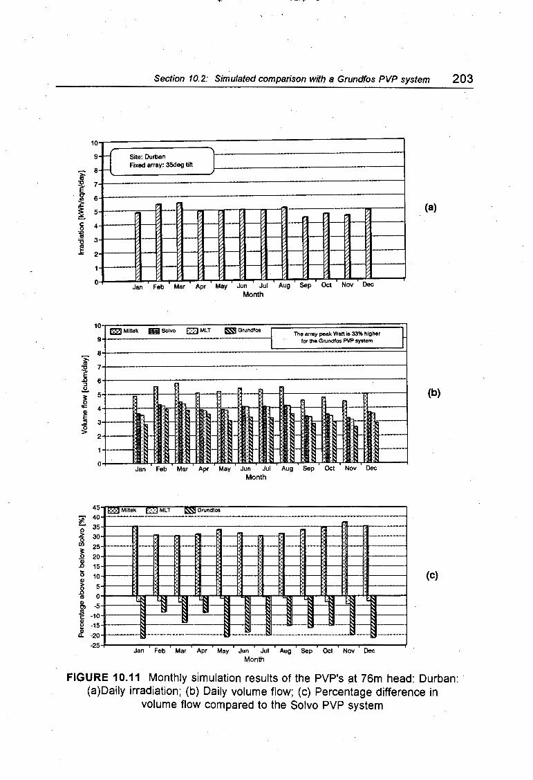
Univers
ity of
Cap
e Tow
n
Section 10.2: Simulated comparison with a Grundfos PVP system 203
i
10
9
8 .tf ' Site: Durban I Fixed array: 35deg tilt J
"C 7 E .[ 6
1 5 (a)
~ 4 co ~ 3
.t 2
0 Jan Feb Mar Apr May Jun Jul Aug Sep Oct N ov Dec
Month
10 IRISolvo EZ'.] MLT ~Grundfos I ~
~Mlltek The array peak Watt Is 33% higher 9 I for the Grundfos PVP system
8
i 7 ::E.
E .D 6 :I ..!:!.
~ 5 (b)
q:: 4 Cl> E r r ' :I 3 ;.._ g t
2 , ,_ '·- ',_ : ..... ,_ "·- .. -
~
0 Jan Feb Mar Apr May Jun Jul Aug Sep Oct Nov Dec
Month
45 ~Miltek t,:,:J MLT ~Grundfos
l: 40
0 35
~ 30 -- -.. _ ·--
] 25
20 ··-
.8 15 .. _
.... (c) 0 10
Cl>
~ 5
co 0
U-- '-R Cl>
j -5 .. ·11:1 __ c -10 Cl> e -15 ---.. Ill
0.. -20 ·~-- .. --· -25
Jan Feb Mar Apr May Jun Jul Aug Sep Oct Nov Dec Month
FIGURE 10.11 Monthly simulation results of the PVP's at 76m head: Durban: (a)Daily irradiation; (b) Daily volume flow; (c) Percentage difference in
volume flow compared to the Salvo PVP system

Univers
ity of
Cap
e Tow
n
204 Chapter Ten: Comparative evaluation and simulations
10.3 Other technical aspects of the PVP systems
This section deals with other technical aspects of the PVP systems which are not directly related to the performance characterisation. System requirements include the availability of components, the maintenance needs of the system and the installation conditions. System attributes include component modularity, flexibility, protection and monitoring.
10.3.1 System requirements
Availability of components
The availability of the system components or parts of the individual components is an important consideration in terms of sustainable water supply from a PV pump.
The PV modules or at least the silicon cells are all imported to southern Africa. Since high quality crystalline modules have an expected service life of twenty years and have become the most reliable component of any type of PV system their future availability is not of major concern.
The Miltek and the ML T controllers have been built in South Africa. The Salvo controller was built in Germany but will in future be produced in Namibia. The electronic components in all the controllers are imported, but since there is a far greater gemeral demand for such components, availability is probably secure.
The Baldor DC motor is imported from the USA. The three phase motor is produced in South Africa.
The progressive cavity Mono pump is produced in South Africa. In addition the company Orbit Pumps also produces progressive cavity pump's.
The Grundfos subsystem is imported from Denmark, through agents in southern Africa, and is presently readily available.
Disregarding the reliability and performance aspect of the four systems the most valuable aspect in terms of availability is to have the components manufactured local.ly (no hard currency loss and support of the local industry). Using that criterion the ML T subsystem is at present completely manufactured in South Africa. The Salvo inverter is intended for manufacture in Namibia.
Maintenance
A maintenance-free PVP system is attractive as it can be used for remote area pumping applications. In my opinion a system that does not require maintenance in a five year period can be considered to be maintenance-free.

Univers
ity of
Cap
e Tow
n
Section 10.3: Other technical aspects of the PVP systems 205
The components of a PVP system that require maintenance are the motor and the pump. They are the only moving parts (except for a tracking array option). The Baldor permanent magnet DC motor requires new brushes every two years.
The three phase motors can be considered to be maintenance-free if the motor drive does not contain any low frequency harmonics or superimposed low frequency oscillations on the line-to-line voltage which can result in torque pulsations. This leads to a shorter motor life-span. The GEC motor could be considered to be maintenancefree if corrected algorithms are implemented in the Solvo and the ML T inverters. An overhaul (which includes a new set of bearings) is recommended every ten years.
The transmission between the motor and the pump is usually via a belt drive. This was the case for these tests. If the pulleys are correctly aligned and the belt tension is neither too low or too high then the belt should last over a ten year period without any breakdown (assuming the operating conditions are conducive, eg, no direct sun and no rain).
The pump will require maintenance or replacement at some stage as a progressive cavity pump has a considerable amount of wear and rotor axial movement. However the time-span is rather indeterminate as each pump element has its own characteristics. Water quality is also an important factor which will have an impact on the life-time of the pump element. The pumps are generally regarded as very durable and reliable with a service life of between five years and twenty years.
The Grundfos motor/pump set would require a service at least every ten years. It may involve motor bearing replacement, pump overhaul and replacements of seals.
All maintenance requirements can be met locally with spare parts being readily available.
Repair
In the case of PVP system break-down, it is most likely that this will occur in the controller (highest number of components, highest degree of complexity). The repair certainly requires skilled personnel.
The Solvo inverter, due to its modular design, is easily disassembled. The power module can be replaced without removing any other components (with a probability of 80% it can be assunfed that the power module has broken down). However, the driver circuit has to be tested to ensure that no damage has resulted due to power module break-down. The Solve inverter can be repaired within one hour assuming that the damage only occurred in the power module and driver stage (repair time based on my experience).
The ML T inverter uses separate power transistors (six) which are not accessible without the removal of the printed circuit boards. Repair from that point of view would require more time. The testing of the driver signals is obscured by the microcomputer

Univers
ity of
Cap
e Tow
n
206 Chapter Ten: Comparative evaluation and simulations
circuit board which would have to be removed. However, since this inverter is a prototype it is recommended for the next generation inverter to change the layout to allow for E~asier access.
No information was available on the repair time for a Grundfos inverter.
Installation
The installation for the progressive cavity borehole pump (Miltek, Solvo and ML T) requires a significant amount of labour and material since the motor is fitted to the discharge head assembly of the pump and transfers its shaft power via a transmission rod to the pump. The installation is therefore fixed and relatively rigid. It requires time to install the pump, connecting the rising main pipes and the rods (half a day to a full day, depending on borehole depth).
The Grundfos motor/pump set is submersible and can be lowered by means of a steel wire and a flexible plastic hose (it can also be attached to iron pipes as above). The time and construction requirements are therefore negligible. The Grundfos system is incomparably easy and quick to install.
10.3.2 System attributes
Modularity
Two levels of modularity are considered. The first level is whether components are separate or integrated and the second level is the modularity within the controller. The latter aspect was discussed in section 9. 7 and is important with regard to upgrading and repairing the controller. In this respect, the Solvo inverter has realised a superior design compared to the Miltek converter and the ML T inverter. No details are available on modularity in the Grundfos inverter (SA 1500).
Component modularity has advantages and disadvantages. All three systems tested are completely modular. The most common combination is to match the motor and the pump into one unit, as with the Grundfos system.
A submersible pump is very easily installed, as noted above, and saves the cost of the cast iron pipes used in the tested systems. Another advantage is the motor cooling due to immersion in water. The disadvantages are the inability to change the speed ratio (the motor and pump are close coupled), the reduction in motor efficiency due to the reduced size and high speed (nominal 3000rpm) and the cost of replacing either the pump or the motor in case of break-down (since both are specialised components).
An advantage of a completely modular system is the ability to replace any one of its components provided the replacement adheres to the specifications. The components are substitutable and can be bought separately. In the case of the Grundfos system the whole subsystem has to be acquired. It might be the case however, that the Grundfos inverter could be used in the three phase systems that were tested (with

Univers
ity of
Cap
e Tow
n
Section 10.3: Other technical aspects of the PVP systems 207
changes in the voltage to hertz relation - not possible without consultation with Grundfos, Denmark).
Flexibility
The tested systems are all quite flexible as they can be used for a range of array sizes and static heads. Adaption is possible by means of different pulley ratios. The frequency range and inverter/motor matching of the three phase systems can be altered in software.
However, these systems are less flexible in terms of re-installing at another site, since removal and installation are time-consuming.
The Grundfos range of PVP systems offers similar flexibility, in covering a fairly wide range (400W to 1800W). However, a particular system will operate best at its design input power and design head. The speed ratio cannot be changed. More sophisticated changes like the frequency range and voltage to hertz relation have to be done in Denmark. This last point requires the customer to buy modules in numbers of eight (as recommended by Grundfos) in order to operate the system at an optimum voltage to hertz relation.
The prototype inverters are more flexible in terms of software alterations by virtue of executing changes locally. The Grundfos system offers the greatest site flexibility since the pump subsystem is a portable unit.
Self-protection
This is an important aspect and has been discussed extensively in section 9.6. A well protected controller becomes more reliable and cost-saving. The protection for both three phase inverters could be improved.
The Grundfos inverter is very well protected. The features include protection against overheating, overload, underload, overvoltage, undervoltage, short-circuit, pump dryrunning and earth leakage.
Monitoring capabilities
Monitoring capabilities are implemented with relative ease in microprocessor based inverters as opposed to analog controllers. However, none of the three tested controllers presently offer diagnostic capabilities or a PVP ~ user interface.
The Grundfos inverter uses LED's to indicate the status of the system. The following conditions are indicated: Overload, underload, maximum frequency, DC power low, overheating, remote switch (pump dry-running or level switch), DC voltage high and DC voltage low.

Univers
ity of
Cap
e Tow
n
208 Chapter Ten: Comparative evaluation and simulations
10.4 Cost analysis
This section evaluates the cost of the Miltek, the Solvo, the ML T and the Grundfos system. This cost is calculated over a period of twenty years and therefore includes all anticipated future costs that will be incurred. In order to compare system costs, the unit water cost is calculated based on the total cost over twenty years and the yearly water delivered, based on results from the simulation package.
Tile initial capital cost of tile systems
Table 10.4 contains the costs of all the components. The prices are specified in current rand (R) which is equivalent to the Namibia dollar (N$).
TABLE 10.4 Costs of components in each PVP system
Component Miltek Salvo MLT Grundfos [R] [R] [R] [R]
Array 1J 12 x M55 (@ R1 399.-) 16 788.- 16 x M55 22 384.-Array structure4
> 700.- Array structure4> 700.-
(Tilt mechanism5> 300.-) (Tilt mechanism5
> 300.-) 10m cable(@ R10.-/m) 100.- 10m cable 100.-
Total 17 588.- Total 23 184.-
Controller 1> 1 404.- 1) 3 780.- 1
> 2 808.- SA 1500 2> 4 764.-
Motor 1> 3 672.- 1) 1 080.- SP 2A - 15 2
> 3 916.-(brushes) 1) 184.- Cable (90m) 2
> 1 170.-
Transmission 31 Piping (90m) 2
> 630.-' Pulley 63.-Taperlock 24.- Total 5 716.-V-belt 17.-
Total 104.-
Pump 3J Discharge head 1 302.-90m pipe 2 235.-90m rod 893.-Bobbin bearings (60) 1 646.-S2M unit 1 188.-
Total 7 264.-
Subsystem cost 12 444.- 12 228.- 11 256.- 10 480.-
Total system cost 30 032.- 29 816.- 28 844.- 33 664.-
1> Prices as per Solar Age Namibia, Windhoek, February 1994 price list
2> Prices as per Namibian Engineering Corporation, Windhoek, February 1994 price list
3> Prices as per Elwiwa, Windhoek, Namibia, February 1994 price list
4> The cost of the Zomeworks tracker is R3 240.-
5> The cost of this item has to be added to the life cycle cost if the simulation assumed a three position tilted array

Univers
ity of
Cap
e Tow
n
Section 10.4: Cost analysis 209
The Zomeworks passive array tracker is not included as the simulation did not include a tracking array. However the prices of two array structures are listed, one fixed and one with the option of adjusting for seasonal changes (10°, 35° and 60°).
TABLE 10.5 Initial installation costs for all four PVP systems
Component Mi Itek Solvo MLT Grundfos [R] [R) [R) [R)
Initial installation Basic 202.- Basic 250.-cost: 3J 90m (R 6.74/m) 607.- n/a
Total 809.- 250.-
3> Prices as per Elwiwa, Windhoek, Namibia, February 1994 price list
Table 10.5 lists the initial installation cost for a borehole pump (as for the Miltek, the Salvo and the ML T system) and a submersible pump (as for the Grundfos system). It does not include travel costs.
The future costs
The future costs are the maintenance and the replacement costs. The replacement costs will always have to include the removal and re-installation costs. The costs are listed in Table 10.6. They do not include travel costs.
TABLE 10.6 Maintenance and replacement costs for the four PVP systems
Description Miltek Solvo MLT Grundfos [R) [R) [R) [R)
Motor maintenance: 4) 4) 2)
Brushes 184.-/ 2yrs n/a n/a Bearings 300.-/1 Oyrs 180.-/10yrs 500.-/1 Oyrs
Pump maintenance: 3)
Discharge head Bearing assembly 702.-/1 Oyrs n/a V-belt 17.-/10yrs n/a Bobbin rubbers 60 units (@ 5.69) 341 . -/1 Oyrs n/a
Total 1 060.-/1 Oyrs
Replacement cost: S2M unit 3> SP 2A -15 2
>
1 188.-/1 Oyrs 1 500.-/1 Oyrs
Removal and re- Basic 202.- Basic 250.-installation cost: 3J Removal 90m (R4.21/m) 379.- n/a
Re-installation 90m ( 6.74/m) 607.- n/a Total 1 188.- 250.-
2> Prices as per Namibian Engineering Corporation, Windhoek, February 1994 price list
3> Prices as per Elwiwa, Windhoek, Namibia, February 1994 price list
4> Prices as per Rolf Rohe, Windhoek, Namibia, February 1994 price list

Univers
ity of
Cap
e Tow
n
21 0 Chapter Ten: Comparative evaluation and simulations
The assumptions in terms of the future costs are as follows: The maintenance requirements for the DC motor are a new set of brushes every two years. All other maintenance requirements and component replacements take place once in ten years.
Realistically the maintenance requirements and the possible component replacements may occur in shorter or longer intervals. This is highly dependent on the conditions under which the system operates. For example the delivery head, the water quality, torque pulsations, current ratings (DC motor brushes) are all factors which will affect the maintenance requirements of the system.
Life cycle cost
The life cycle cost (LCC) calculates all the anticipated costs that are incurred over a particular project lifetime. It includes the initial cost and all future expenditure. Appendix A9 gives a detailed description of the method of calculation and the equations used.
Table 10.7 lists the LCC for the four PVP's under discussion. The project lifetime is taken as twenty years (SL = 20), the real discount rate is 5%, the rate of escalation is assumed to be zero percent and the real interest rate is assumed to be 5%.
The initial cost for each system is taken from Table 10.4 and Table 10.5. The maintenance and the replacement costs are taken out of Table 10.6. For each replacement interval the pump or the motor/pump set have to be removed and reinstalled. This cost is also listed in Table 10.6.
All amounts listed in Table 10.6 are reduced to their present value by incorporation of the discount rate and the time at which the cost occurs.
TABLE 10.7 Life cycle cost of the four PVP system with a project life of 20 years
.PVPsystem Life cycle cost [R]
Miltek 34 144.-Solvo 32 739.-MLT 31 767.-Grundfos 35 230.-
1> The LCC of the Grundfos system includes
the cost of sixteen modules where the other systems only use twelve modules
The Grundfos system has the highest LCC which is due to its larger array. The Miltek system has the second highest LCC which is mainly due to its motor maintenance requirements if compared to the Salvo and the ML T system. The Salvo system costs R1400.- less than the Miltek system. The MLT costs about R1000.- less than the Solve system which is due to price difference in the inverters as all the other costs are the same.

Univers
ity of
Cap
e Tow
n
Section 10.4: Cost analysis 211
Unit water cost
The unit water cost (UWC) is the most relevant costing parameter as it incorporates the system performance. The equation by which it is calculated is in appendix A9.
The unit water cost has been· evaluated at two sites, namely Windhoek and Durban and for two types of array structures namely fixed and three position tilted array. The conditions under which the simulations took place are listed in appendix A8.2.
TABLE 10.8 Unit water cost for all four PVP systems
PVP Unit water cost {centslm3]
system Windhoek Durban
three position fixed three position fixed tilted array 1> array tilted array 1> array
Miltek 100.1 103.8 140.4 146.7
Solvo 118.7 124.8 177.6 186.8
MLT 116.0 122.4 176.0 185.1
Grundfos 126.9 136.7 219.5 240.8
1) The three angles of tilt are: 10° for Nov - Feb; 35° for Mar - Apr and Sep - Oct; 60° for May - Aug
TABLE 10.9 Hydraulic unit water cost for all four PVP systems at 76m static head
PVP Unit water cost [centslm'} system
Windhoek Durban
three position fixed three position fixed tilted array 1> array tilted array 1> array
Miltek 1.32 1.36 1.85 1.93
Solvo 1.56 1.64 2.34 2.46
MLT 1.53 1.61 2.32 2.44
Grundfos 1.67 1.80 2.89 3.17
1) The three angles of tilt are: 10° for Nov - Feb; 35° for Mar - Apr and Sep - Oct; 60° for May - Aug
Due to the higher performance of the Miltek system it manages to achieve the lowest UWC although the LCC is R2400.- higher than the cheapest PVP system, the ML T system. The Solvo and ML T systems have similar UWC. The UWC of the ML T system

Univers
ity of
Cap
e Tow
n
212 Chapter Ten: Comparative evaluation and simulations
is slightly lower than the Solvo UWC as it has a lower LCC which makes up for its slightly poorer performance compared to the Solvo system. The UWC of the Grundfos system is the highest as its performance did not meet up to the other three systems while its LCC is the highest. Compared to all the other systems the Grundfos UWC increases disproportionately when operating under Durban weather conditions. The UWC increases by over 70%. This is due to its drop in efficiency when it receives comparatively less power on average.
The UWC for all systems is likely to decrease when a tracking array is used. The LCC would increase by 7.2% to 8% (cost of the tracking array less the fixed array divided by the LCC) while the annual water output will increase by more than that percentage. A rough estimate for the Miltek system could be considered to be 20%. As shown earlier, the gain of a tracking array for the three phase prototype systems will be larger. It was also argued that the Grundfos PVP would benefit even more than the prototype three phase systems due to the sensitivity of the subsystem efficiency to the input power. The conclusion of this deliberation is that the relative gap between the UWC cost as it has been evaluated will decrease when a tracking array is used.
Further simulations show that the UWC of the Grundfos system drops substantially if the system is configured with 3 x 8 modules (equivalent to: 24 modules Wpeak of 1271W and LCC of R46 721.-). Its UWC at the Windhoek and Durban site with a fixed array is 87.8c/m3 and 133.4c/m3 respectively. Unfortunately, data for the other three systems is not available at these array sizes. However, their UWC is likely to decrease as well since inverter efficiency and motor efficiency will improve (the efficiency of induction motors increases with higher power ratings; both increases are marginal though). In comparison, it is possible that the UWC of the Grundfos system would reach similar magnitudes to the UWC of the three phase prototype systems or perhaps even be lower. This is mainly due to the subsystem performance improvements as the Grundfos PVP moves towards its design power.
All considered, the Miltek PVP system, followed by the Solvo and ML T PVP systems perform superior to the Grundfos PVP in the sub-kilowatt region (fixed and three position array) at a static head range of ?Om to 80m.

Univers
ity of
Cap
e Tow
n
Chapter Eleven
CONCLUSIONS
Photovoltaic water pumping for remote deep wells can be efficiently implemented with a progressive cavity pump in the higher sub-kilowatt region. These pumps are widely used in southern Africa and are driven by wind, diesel, grid or PV power sources. Some of the advantages that PVP's offer over wind and diesel pumps are that they are virtually maintenance-free with zero operating costs, relatively modular, potentially better synchronised to the water supply in the borehole and able to operate autonomously. The major disadvantage is the high initial capital cost. The photovoltaic array makes up a large portion of initial costs, and there are limited economics of scale, with increasing power (unlike diesel pumps, which therefore become more competitive for larger pumping requirements).
Review
Two prototype three phase PV pump systems and a DC PV pump system were tested on a farm (Latitude: 21°6' and Longitude: 17°6') in Namibia, 1 OOkm north of Windhoek. The array consisted of twelve modules (636Wpeak) mounted on a single-axis passive tracker. The depth of the water level was 75m and a progressive cavity pump with a self-compensting stator was used.
The field tests were conducted from February 1993 to June 1993. The time prior to testing was spent designing measurement circuitry for the primary data acquisition system and preparing test procedures. The primary data acquisition system was mainly used for the data collection of steady state PVP signals. A secondary data acquisition system was used to capture instantaneous samples of higher frequency signals.
The emphases of this study was to assess the performance of each system and its components under various operating conditions, to observe the response of the controller under transient conditions, to evaluate possible weaknesses in the systems which might lead to break-down and to make concrete suggestion towards the development of the Solve inverter. In addition, the prototype systems, the DC system and a three phase Grundfos system were compared using a simulation program.
The collected data was presented instantaneously for each component or set thereof but was also processed to a more comparable level by looking at the daily performance and evaluating the daily energy efficiency over a standard solar day. The uncertainties for the collected data were reported in the main text and all the figures quoted here are subject to the uncertainty margins quoted earlier.

Univers
ity of
Cap
e Tow
n
214 ·Chapter Eleven: Conclusions
I i
Overall performance and costs of the eval.uated PVP systems I
The DC PVP system tested in this study performed better than the three phase prototype~ systems. Under test conditions the subsystem efficiency of the Mi Itek system reaches a peak 42%. The ML T and Solve subsystem efficiencies reach a peak: of 35% and 33% respectively. Over the whole operating range, the Miltek subsystem e~iciency remains approximately 7% above the three phase subsystems' efficienqy. The operating range of the Miltek system is wider than that of the three phase systems, starting at SOW array power while the Solve system and ML T system start operating at 160W and 180W respectively. ,
• ' i
The system daily energy efficiency for a 5kWh/m2/day and. a 7kWh/m2/day a~e listed below: ·!
Miltek [%] Solvo [%] MLT [%]
5kWh/m2/day 3.6 2.6 2.1
7kWh/m2/day 4.2 3.2 3.2
The difference between the Solve and the ML T system at 5kWh/m 2/day is due to higher subsystem efficiency of the Solve system at lower array input pow~r. The system DEE of the ML T PVP improves with respect to the Solve system as the] energy content .of the standard solar day increases as can be seen for 7kWh/m2/day.
Simulations were conducted with the tested systems (636W peak arra) and a Grundfos PVP system (SP 2A-15, 848W peak arra) for a fixed and a three position tilted c;trray at a static head of 76m. The simulation was performed at two sites, namely Windhoek
I
and Durban. The annual average irradiation received in Windhoek is 6.9kWh/m2/day while Durban receives 5kWh/m2/day. It was found that the average performancb of the Grundfos system was below that of the three tested systems at both sites. The difference was more marked at the Durban site where the Grundfos system performed poorest. It can be observed that the performance of the Grundfos system improves rapidly during days of high irradiance which is characteristic of centrifugal p~mps.
The unit water costs were calculated from the amortised life cycle costs ~nd the annual water flow. They are listed for the fixed array at Windhoek and Durban:
Miltek Solvo MLT Grundfos [c!m3J [c!m3J [c!m3J [c!m3J
: Windhoek 103.8 124.8 122.4 136.7
Durban 146.7 186.8 185.1 240.8
(The poor performance of the Grundfos system is due to operating at nont optimal array peak power. Simulations where the array size was increasetj showed a marked improvement in the unit water cost of the Grundfos system.)

Univers
ity of
Cap
e Tow
n
Conclusions 21 5
Array performance
The array performance was measured to be somewhat lower than the values specified in the module data sheets. Measured performance fell just outside of the ±10% range of the module specifications. As the performance of the array was based on the measurements of all modules combined it is expectable that the performance would be lower than the performance of a single module due to mismatch losses. In addition, the uncertainty in the measurements was higher than 13%, making an assessment of the array performance compared to the specifications impossible. However, this high uncertainty stems from the input measurement to the array. The array output can be assessed accurately and therefore does not compromise accurate evaluation of the subsystem.
The cell temperature has a marked effect on the performance of the array, and a PVP system operating at a fixed array voltage can lose substantial amounts of power if set to an inappropriate array operating point. Array measurements showed that if it was 47°C there would be losses of 7% if the system operated at 200Varri 3% at 195Varr and about 2% at 190V arr• relative to optimum power. The data demonstrated that it is more beneficial to operate at a lower array voltage set-point rather than a higher set-point as the losses incurred due to operation at relatively low array voltage are lower than at high array voltage assuming large variations in the cell temperature.
The benefits of the tracking array were evaluated for a particular time of year. It was found that the passive tracking array received 12% more solar energy than the fixed array. The difference is small due to the time required by the passive tracking array to move from a west-facing position to an east-facing position in the morning. An active tracking array was simulated (it faces east before the sun rises in the morning) and was found to receive about 23% more solar energy than a fixed array under test conditions.
Pump performance
The pump performance was as specified although the operating point at which the maximum efficiency occurred did not coincide with the specified operating point. The flowrate was about 5% lower than the specified flowrate. However the uncertainty in the flowrate measurement is 6.1 %. The torque-speed characteristics were found to be non-linear with a pronounced discontinuity occurring at mid-operating range (500rpm to 600rpm). The torque rose exponentially at that point and then dropped steeply to a lower torque. This was found to be a known phenomena which is due to the selfcompensating stator element of the pump. This characteristic did not affect the flowrate considerably. It does however demand a torque from the motor which may not always be generated efficiently over the complete operating range of the PVP system.
Compared to pumps from Orbit, the Mono S2M pump was the best choice considering the static head and the input power range.

Univers
ity of
Cap
e Tow
n
216 Chapter Eleven: Conclusions
Controller and motor subset performance
Since the switching frequency of the controller has an impact both on the controller efficiency and on AC motor efficiency it is more representative to either component to discuss the performance aspect from a combined efficiency point of view, that is the subset efficiency.
For an array output power range of 200W to 500W, the Miltek subset efficiency ranges from 60% to 78%, the Salvo subset efficiency ranges from 40% to 60% and the ML T subset efficiency ranges from 40% to 65%. The subset efficiency of the Miltek system exceeds tl1e subset efficiency of the three phase systems over the whole range. The ML T subset efficiency is poor in the 200W to 350W array power region which is mainly due to poor motor efficiency. This may be the result of a high harmonic content in the current waveform. In addition, the voltage to hertz relation is disturbed by high variations in the array voltage operating point during maximum speed tracking mode which alters the reference voltage substantially. However, the ML T subset efficiency is slightly higher than the Salvo subset efficiency at array powers in excess of 350W.
Assessment criteria of tile prototype three phase inverters
Although much emphasis was placed on the efficiency evaluation of the inverters, it was realised that the reliability aspect of the inverters was crucial. Efficiency is essential but system reliability is paramount as PVP's find good application in remote areas which thus requires reliability. It was therefore considered a priority to evaluate inverter reliability and suggest improvements in that respect. As a second priority the inverter efficiency was considered with suggestions made towards software alterations which would improve efficiency. Hardware alterations for that purpose were not considered.
Assessment of tile Solvo prototype three phase inverter
The main findings were in the areas of inverter algorithm capabilities, inverter output waveform quality, inverter efficiency losses, inverter protection and inverter diagnostic capabilities.
Control algorithm
The control algorithm which decides whether the motor speed is increased or decreased was found to be incapable of operating at a fixed voltage. Instead the array voltage oscillated around a mean value. The system was therefore stable but did experience array power losses due to voltage swings in the order of ±1 OV to ±1 SV. This behaviour also had an impact on the line-to-line voltage applied to the motor resulting in a non-optimal voltage to hertz relation and torque pulsations. In addition, the monitoring of system operating states (for example, a low array operating voltage point) would be made difficult as a simple threshold value would not suffice. A mean of the particular parameter would have to be sampled. Suggestions towards an improved control algorithm are in section 9.1.

Univers
ity of
Cap
e Tow
n
Conclusions 217
Operating states algorithms
The operating states algorithms were found to be incomplete. The system would therefore get into operating states that were either unproductive (eg, no water pumped) or could possibly result in inverter breakdown. The most basic operating state algorithm which was not implemented was an algorithm monitoring a bottom threshold of the array voltage. It was therefore possible to find a system operating at half its set operating voltage. Instead of performing a restart the system was stuck in this state. Algorithms which avoid unproductive operating states are presented in section 9.2.
Quality of the output waveforms
The inverter generated a sinusoidal PWM signal at high switching frequency. Due to the array voltage oscillations, the rms voltage had a superimposed low frequency ripple which resulted in 4 - 8% amplitude variations. In terms of variable voltage control, the resolution of the rms voltage was poor in that only ten different amplitudes were programmed for the frequency range from 6Hz to 85Hz.
The inverter produced a high quality current waveform in the windings of the motor due to its sinusoidal PWM switching scheme and its high switching frequency. The waveform quality did not degenerate at low operating frequencies due to these switching characteristics.
Efficiency improvements
It was found that the voltage applied to the motor over the full operating range was changed in a series of large steps. This undermined efforts at an optimal voltage to hertz relation. Improving the resolution would improve the subset efficiency (section 9.3), assuming that the optimal voltage to hertz relation is known. It was also suggested to perform tests on the subset efficiency of a Salvo inverter, with a ·lower switching frequency range which could reduce switching losses (section 9.4).
Inverter protection
The inverter was protected against short-circuit on the inverter output, overload, noload and overheating. Further protection would involve protection against lightning, polarity reversal, overvoltage and pump dry-running.
General assessment
In general the reliability and possibly the efficiency of the Solvo inverter will improve with the implementation of the suggestions made in chapter nine. The dedicated PWM IC used by the Solvo inverter proved to be somewhat inflexible as it could not overmodulate the output voltage to generate a higher line-to-line voltage. On the other hand, this particular IC protects the power module as bus shoot-through (both switches on at the same time) is not possible with this type of digital drive circuit hardware.

Univers
ity of
Cap
e Tow
n
218 Chapter Eleven: Conclusions
The power for the drive circuitry and the microcomputer was supplied from a swikhed-mode power supply which is more efficient than a linear voltage regulator. '
i
No user interface was offered in this prototype inverter. As these are relatively inexpensive, a user interface should be considered once the software requirements and development time have been assessed. However, this may not be a viable bption if the potential market is not big enough to justify this type of addition to the inyerter. ·
I
The physical layout of Solve inverter is to be recommended as it proved :to be extremely modular thus making hardware and software upgrades simple and rast.
Assessment of tile MLT prototype tliree pliase inverter
The main findings for this inverter were in the area of fixed voltage operation (FVO) and maximum speed tracking (MST) algorithm capabilities, inverter output signal waveform, inverter protection and inverter diagnostic capabilities. '
Control algorithm
The basic control algorithm for both FVO and MST operation was implemen~ed in exactly the same way as the algorithm in the Salvo inverter. The conclusions regarding the basic decision making of the inverter were therefore the same. However, it was also observed that the ML T inverter in FVO mode had a very narrow ope~ating range. This point requires further investigation as the system cannot be operated
I
economically in this operating mode. :
The MST program presented tuning difficulties as the maximum speed set~point interfered with the start-up threshold of the system. A particular set-point might for example prevent the system from leaving its base speed (a low speed operatiorh with no water delivery) until a 600W/m 2 solar irradiance level was received. Another setting might result in start-up at 450W/m2
. The maximum speed was therefore rever optimised but the start-up threshold was lowered as much as possible.
Operating states algorithms
This inverter was unable to distinguish between useful states of operation and I
unproductive states of operation. Both programs (FVO and MST) exhibited similar characteristics in that respect. Like the Solvo inverter, the ML T inverter could lose its operating point and 'operate' at less than half the array voltage set-point. As th~ lineto-line voltage applied to the motor under these conditions was far too low, the motor stalled since it could not draw sufficient current (from the capacitors and the array) to maintain the torque at such low array voltage and inverter oputput voftage. Suggestions to avoid this behaviour are in section 9.2.
The reset circuit which is activated in MST mode resets the controller when the motor does not turn. In principle the idea i~ good but the problem is that the microcontroller restarts immediately. Instead of losing control over its state of operation the
I

Univers
ity of
Cap
e Tow
n
Conclusions 21 9
microcontroller should rather inhibit its output and enter a wait state. This essentially involves a change from a hardware implementation to a software implementation.
The inverter progresses through a number of non-e.ssential operating stages as it starts up and as it comes to halt. These states are unproductive and can be avoided with proper monitoring as suggested in section 9.2.
Quality of the output waveforms
The inverter generated two types of PWM switching schemes namely sinusoidal and harmonic elimination PWM. The sinusoidal PWM scheme is suitable for low speed operation and the harmonic elimination PWM scheme improves the inverter efficiency due to a reduction in required switching while still applying a PWM waveform to the motor that is free of undesired low frequency harmonics. Both schemes were implemented, with sinusoidal PWM at low operating frequency and harmonic elimination at higher operating frequency.
The inverter is capable of overmodulating its output voltage signal which has the benefit of generating higher voltages from the available DC voltage than a strictly sinusoidal PWM signal. However, overmodulation has a negative impact on the harmonic spectrum.
The resolution of the variable voltage signal was good being nineteen amplitudes over an operating range of 3Hz to 65Hz.
Due to the array voltage oscillations, the rms voltage had a superimposed low frequency ripple which resulted in 8 - 13% amplitude variations.
The inverter produced a current waveform in the windings of the motor which was of reasonable quality. However, due to its low overall switching frequency, the current waveform was slightly distorted indicating the presence of large amplitude and low frequency harmonics, apparently leading to reduced motor efficiency.
Inverter protection
The ML T inverter offers hardly any protection except for a power supply fuse. It is therefore recommended that the inverter be protected against lightning, polarity reversal, overvoltage, phase short-circuit, overload, overheating and pump dry-running.
General assessment
The inverter achieves a comparatively good efficiency due to its sophisticated PWM switching scheme which is generated directly out of the ports of the microcontroller. Efficiency could be improved with a more efficient power supply (that is a switchedmode power supply). The general algorithm implementation is too simplistic and requires a more complex controller. These aspects are discussed in sections 9.1 and 9.2.

Univers
ity of
Cap
e Tow
n
220 Chapter Eleven: Conclusions
The principle of ~aximu~ speed tracking could possibly be changed to ma~imum power point tracking using the same algorithm. It may however be advisable to perform analog multiplication as this provides a continuous signal to the ADC and does not have any phase-shift problems as may be the case with software multiplicatio~. Thi~ would ~void the use of an external sensor like the speed sensor. However, this option requires detailed investigation. :
i I
A user interface was not available for this prototype inverter. It would be recommended if the demand ~or such PV pump inverters is high enough to justify this type of development. Should 1t be found that a user interface is not justifiable then a panel of status LED' should be integrated into the design. :
The physical layout of the inverter poses accessibility problems and the strubtures holding the PCB's are clumsy. Replacing a MOSFET took about an hour as all bircuit boards had to be removed. The potentiometers for array voltage · and speed adjustments were placed in the plane of the PCB. They should be top adjustment-type potentiometers. i
I
I
Concluding comment '!
This study evaluated two prototype AC pumping systems and compared them ~ith an established DC system, in a subkW deep borehole application (636Wpeak• static: head of 75m and about 0.069m4/day to 0.083m4/day). ! I
:
With switching schemes like those implemented in the ML T inverter, low powe~ drive circuits, single chip microprocessor boards, higher power supply efficiency que to switched-mode power supplies and improved motor design, a three phase system could become an attractive alternative to the DC system. In addition, the three phase systems could be offered at a better price since the motors can be produced lqcally. Monitoring capabilities and some form of interaction with the user can be standard features. However, it is unlikely that the performance of the three phase systems will improve beyond that of a DC system due to higher drive circuitry requiremen~s and generally lower subset efficiencies in this power range. If the switching frequentjy and the voltagE~ to hertz relation have been optimised with a particular motor and if the motor itself has been optimised for efficiency then a three phase system could achieve I
a peak performance that is possibly within 3% of the current peak subsystem efficiency (42%) of the Miltek DC system. Cost factors, maintenance requirements and potential local production could then favour a three phase system.
• I I For larger PV pumping systems (in the kW range), the AC systems have a. more established place, mainly due to the cost, size and limited availability of suitable. high- · power DC motors. Grundfos submersible AC pumpsets (using centrifugal pilimps) extend into the kW range. However, simulation comparisons with a Grundfos PV :pump system (SP 2A-15, 848Wpeak• centrifugal pump) indicated that the three tested system, using progressive cavity pumps, had a superior performance in the subkW region.
:

Univers
ity of
Cap
e Tow
n
Chapter Twelve
REFERENCES
Anand, D K (1974). Introduction to control systems. New York: Pergamon.
Baltas, P & Russell, PE (1987). The dynamics of PV water pumping. Nineteenth IEEE Photovoltaic Specialists Conference, 1031-5.
Borchers, M L (1992). Considerations in assessing the economic viability of standalone photovoltaic systems relative to other supply options. Engineering Professions Association Conference on Solar Energy, Windhoek, Namibia.
Bose, B K (1986). Power electronics and AC drives. New Jersey: Prentice Hall.
Burton R (1992). PV water pumping - The Botswana experience. Engineering Professions Association Conference on Solar Energy, Windhoek, Namibia.
Cowan, W D (Ed) (1992). RAPS design manual, Volume 1. Energy for Development Research Centre, University of Cape Town, Cape Town.
Davies J L (1992). The design and optimisation of a system using an induction motor driven pump, powered by solar panels. MSc. Dissertation, Elec Eng, University of Cape Town.
Davis M (1993a). Photovoltaic pump handbook. RTU Report Series 1, Energy for Development Research Centre, University of Cape Town.
Davis M (1993b). Directory of PV pumping equipment. RTU Report Series 2, Energy for Development Research Centre, University of Cape Town.
Davis M (1994a). PVPump - A user's manual. Energy for Development Research Centre, University of Cape Town. ·
Davis M (1994b). Simulation of PV pumping systems. Energy for Development Research Centre, University of Cape Town.
Gosnell R J (1991 ). Photovoltaic water pumping - A case study in KwaZulu. MSc. dissertation, Energy for Development Research Centre, University of Cape Town.
Halcrow W (1983). Small scale solar powered pumping systems: The technology, its economics and advancement. Intermediate Technology Power, Sir William Halcrow & Partners, UNDP Project GL0/80/003, Executed by the World Bank, London: Swindon and Reading.

Univers
ity of
Cap
e Tow
n
222 Chapter Twelve: References
Herrmann B, Karl H, Kopf E & Lehner G (1987). Realistic indoor testing of photovoltaic water pumping systems. Solar Energy, Vol. 38, No 4: 275-9.
Hexfet Power MOSFET Designers Manual (1987). 4th edition, International Rectifier, California.
Hirschmann G (1989a). Leistungshalbbrucke fur Drehstrommotoren mit IGBT BUP 304. Der Elektroniker, No 12: 27-30.
Hirschmann G (1989b). Sinustabellenprogramm 'Sinus' mit Turbo-Pascal fur das PWM-Konzept. Internal report, Siemens Bericht No 8902 PD11.
Holman J P (1978). Experimental methods for engineers. 3rd edition, New York: McGraw-Hill.
Horowitz P & Hill W (1989). The art of electronics. Second edition, New York: Cambridge University Press.
lliceto A, Piazza V & Guastella S (1987). Long-term comparison between two-axis and single axis tracking PV systems and a fixed PV array. Nineteenth· IEEE Photovoltaic Specialists Conference, 238-42.
Kitchin C & Counts L (1986). RMS to DC conversion application guide. Second edition, Analog Devices, USA.
Lasnier F, Gan Ang T, Lwin K S & Hemasuk T (1988). Photovoltaic tests and instrumentation - Pumping system. Energy Technology Division, Asian Institute of Technology, Bangkok, Thailand.
Lasnier F & Gan Ang T (1990). Photovoltaic engineering handbook. Bristol: Adam Hilger.
Mohan N, Undeland T M & Robbins W P (1989). Power electronics: Converters, applications and design. Singapore: John Wiley & Sons. ·
Murphy J M D & Turnbull F G (1988). Power electronic control of AC motors. Oxford: Per~~amon.
Payne S A E (1986). The design and production of solar powered positive displacement pumping systems. Unnumbered conference paper, Renewable Energy Potential in Southern Africa Conference, Energy Research Institute, University of Cape Town, 8-10 Sept.
Schaefer J F (1985). Results of a survey of 111 photovoltaic water pumping systems in New Mexico. New Mexico Solar Energy Institute, Las Cruces, New Mexico.

Univers
ity of
Cap
e Tow
n
References 223
Scholey D (1982). Induction motors for variable frequency power supplies. IEEE Transactions on Industry Applications, Vol 1A-18, No 4, July/August.
Schmalschlager T, Piernavieja G & Kranz G (1993). Sonnenstandsnachfuhrung -Theorie und Praxis bei kleinen PV-Anlagen. Sonnenenergie, No 3: 8-11.
Schmid J (1987). Recommendations for measurements on inverters. European PV Plant Monitoring Newsletter, Commision of the European Community, Number 2, July 1987.
Vetter G & Wirth W (1992). Exzenterschneckenpumpe - Einsatz in der Photovoltaic. Sonnenenergie, No 3: 12-9.
Vetter G & Wirth W (1993). Suitability of eccentric helical pumps for turbid water deep well pumping in photovoltaic systems. Solar Energy, Vol 51, No 3: 205-14.
Whitfield GR & Bentley R W (1988). The efficiency of small scale solar photovoltaic water pumping systems. International PV Conference, 1123-6.

Univers
ity of
Cap
e Tow
n
Appendix A1
PV PUMP COMPONENT SPECIFICATION SHEETS
A 1.1 Siemens M55S module
Installation advice The following minimum distances must be observed in order to ensure sufficient rear ventilation of the module: - from the rear walls >50 mm - from the neighboring modules
>5mm
Recommended minimum slope 15°
Installation from the rear is facilitated by M 6 nuts pressed into the frame.
The wiring of the modules is accomplished via plastic cable bushings in two plastic terminal boxes attached to the back; one positive, one negative. One of the boxes is clearly marked with a"+" to designate the polarity.
Measurements
-~ ~
-i-ODO 0
1 ~ i!!
J 4xM6 /
mo 0
~332-l 3-211- l-31s-ll::.8
Internal Circuitry Bypass diodes (in the terminal box) protect from "hot spot effects" preventing possibl.e destruction if the module is partly shaded.
Siemens Solar GmbH A joint venture of Siemens AG and Bayernwerk AG
Thermal parameters:
11 These values are subject to a manu-facturing de~iation of plus/minus 10%.
21w0 Watt peak= peak output under . standard testing conditions: Airmass AM=1.5 lnsotation E=1000W/m2
Cell temperature Tc= 25°C
r-----------------, I I I I
I I I I
1 ' 3 ------- 12 J
L-----------------~
.. ,.·,:
+4x10⁻⁴/K
- 3.4x10⁻³ /K
·-;. :. .-: > .~.):·.~ ... ~.-~-
·.·.I
.. '··· _:-::·_::
3J Normal cell operating temperature at: lnsolation E = 800 W/m2
Ambient temperature Tu =20°C Wind speed Vw=1 mis
Current voltage characteristics
3S
JD
2.S
2D
1S
•D
OS
0 0
1000Wlm',•T-C (NOCT') -- -1000W/fl'l2,25"C,
I I I ~ \ I I I ' ,
500Wlm2,25"C
I I i !'-100Wtm',259C I \
I I ' l1 12 16 20 .. 24V
Subject to technical alterations
Frankfurter Ring 152 8000 Munich 40 Tel. (0 89) 35 00-2411 Fax (089) 3500-2573
\'.55~090GB02DAT

Univers
ity of
Cap
e Tow
n
228 Appendix A 1: PV pump component specification sheets
A 1.2 Zomeworks TRPM12/AR passive solar tracker
·'1
i' '11 " <I : I
TRACK RACK™ Passive Solar Tracker for Photovoltaic Modules
OJr Fl:Jsslw Solar TRACK RACKSN opet01e by liquid llowlng be1-'I sealed frame memben. 1hel9 are no drtw motoo. gears oi ( pistons; ll'lel8 is llttle to wear out. The Zomeworks Fl:JaMI Solar TRACK RACKSN areasdependabteasgrovttyand the heatofthesui.
TESTS CONDUCTED OVER A 12-MONTH PERIOD BY NPN MEXICO STATE UNIVERSllY AT 34" N LATflU)E SHOMO AN IMPROVEMENT IN ELECTRICAL OUTPUT BV TRACklNG AROUND AN ADJIJSTABl1: N-S AXIS Of 29'l> OVER A AXED LATflU)E MOUNT. lHE IMPROVEMENT RANGEDFROM19'1.INNOVEMBERT042'r.INJUNEANDJULV.lHISIVEANSTHATUSINGANEIGHT-MODUlETRACKRACK"'ISUKEHAVING 1.6 EXTRA MODULES IN lHE WINTER AND 3.2 IN 1HE SUMMER. OR AN A~RAGE Of 2.3 EXIRA MODULES FOR lHE VEAR.
The Zomewaks TRACK RACK"' Is Ideal for stock 'Mllertng or lrrtgal1on. On a clear summer day. photo\loltale moduleS mounted on oui l1tlcker will dell\ler 55'1. more enetgy than moduleS on a fl>Bd latftude mount The solar eleCtrlc power comes In a smooth dawn-todusk flaw rather than a noon peak. lhls enableS 55'1. more wc1er to be pumped on the hOttest days of the yearwtthout purchasing additional modules or a laiger pu!'r4:).
The ZomewOlks TRACK RACK"' ls constructed of painted mild steel. Stainless steel lt:ldc.sare0110llable. The TRACK RACK"' ls designed to withstand :JO lbs/sq fl wind loading. Specially-made shock ab90lbers dampen mot10n In high winds. I
The TRACK RACK"' Is easy to Install. It slips over a pipe most set In concre1& and Is IOcked Into place by tlgh!&ning one bolt. I The N-S axis is seosonolly adjustable for top peitormonce an year long. I
I US Plltent •4,275,712

Univers
ity of
Cap
e Tow
n
Section A 1.2: Zomeworks passive solar tracker . 229
TRPM12/AR
86" 66n
' 5" SCH 40 PIPE :I (5 9/16n OD)
I~
TECHNICAL DATA Model TRPM02/AR TRPM04/AR TRPMOl/AR TRPM12/AR TRPM14/AR
Number of Modules 1or2 4 8 12 14
Maximum Module Area (sq ft) 9.5 18.5 37 55.5 64.5
Rock Dimensions (inches) 28X52 51.5 X68 59X117 86.5X 115 100 x 121
Mounting Mast (height from ground) :Y1' IC' 56" 66" 74'
' Ape Sim (Sch 40) steel 'l' 2.5" 4' 5" ti'
Actual Pipe OD 2.375" 2.875" 4;5" 5.563" 6.625"
Shipping Weight (lbs) 50 80 130 180 210
Angles Axis Adjustment 5-45• s-45• s-45• 5-450 5-45"
Tracker Groves Max N-S Spacing NA 15· 20· 30· Y1 Max E~W Spacing (approx) NA 20· 20· 30· 35· -
Price

Univers
ity of
Cap
e Tow
n
230 Appendix A1: PV pump component specification sheets
A 1.3 Mono S2M borehole pump
SOLAR
SONKfiAG
MONO PUMPS. PUMP SIZE
POMP GROOTTE 5 2 M TYPICAL AVERAGE PERFOP.MANCE
TIPIESE GEMIODELOE POMPPRESTASIE MAX HEAD 150m MAX SPEED ·1200r/min
MAKS HOOGTE• MAKS SPOED
l.OmmCOLUMN 13mmSHAFT UP TO 150m l.Omm PYPE 13mmSTANGE TOT OP 150m mm COLUMN mmSHAFT UP TO m mm PYPE mmSTANGE TOT OP m
MONOSTROOM DISCHARGE HEAD UP TO 150 m tv!0i'!05TROl')tv: ONTSLAGKOP TOT OP 150m DISCHARGE HEAD UP TO m ONTSLAGKOP TOT OP m
MINIMUM STARTING TOROUE 3N.m Ml NIMUM DRAAIMOMENT
:_.i ~ ~- .i:: :...,.,_: .. , ..... -'.i c:+:c :_:_l_IJ_: .. -+·· ~!::.: .. _: ~..:: :..+-· ··+:_ :j:::: .i:.[.._I'-" 2, ~~~g (r/min)
o .... 1 ..... ····I····±_ .. , .... -·· _,_ -··1·- ·- .... _ . .1. .... '-+- .... ,. __ ,_1...._ .... , .... __ , __ , ·--'···· c. ... '"""
~ :: =i==:=c:;c'=r=:-=1=*=8-:;:_:£:_ ~~~~±::: c!. ·-·-·· ~- ·-+-,. -,.. - -·+·· ·-- -- --.. ·- ····1·-·~ ~._kb: -1-'C-W .. ·····-
0.1. •: l :: .. . :, , .. . . .· • ! : , * I . '. :: • ::. : ::' . ··. I~ : :· .-; : •• I~ 680000 .... ··- :1 .. , •.. ! ...... :·:: ..... I ;.. .. !:.. ... I : I
I .. /." .. I ·I . .... ..... LOO 0.2 ' I t ' ' ' <f' I ' ••. I .·-·r··· •••••• ' 200
-.... · 1200
. . 800
· ::-t-:-,!- GOO
I .. ,. - .,.
.....
: I .. I I 1'· ; I : : ... · ... ,.. . ,-...;;;...__ I . ~I i .... I . -· ' ' ' I ' -.__ .. .. . . . - 20Q
0 110 LU 5(1 Al' 101J 120 ILO
!~S~C :,n 1 :;>:,!'f: 01·09·80 CURVE NOC 270

Univers
ity of
Cap
e Tow
n
Section A 1.4: Solvo circuit breaker and po;.,er module
A 1.4 Solvo circuit breaker and power module
A1 .4.1 Thermal three phase circuit breaker Mbs 25
Motor Protective Switch Specification Motor protective switch complys with .. Agreement for Low Vottage Switchgear" to DIN 57 660NDE 0660 and the IEC Publication 292-1 and 157-1. When incorporated in the insulated enclosure, front plate, and with the emergency stop mushroom pushbutton it also complies with VOE 0113 for Main, and emergency disconnect switches.
Operating mechanism Manually operated by pushbuttons, with a positive trip free feature. Clearly visible switch position indication, and positive contact separation. Available with padlocking facility in the .. Off .. position, accommodating up to 3 padlocks, with bow thickness of 6-8 mm, when used in insulated enclosure type i, or frontplate type it.
Trip device Thermal overload trip "b" Triple pole. adjustable. motor protection characteristic (trip characteristic T II). Single phase fautt sensitivitJ, and ambient
Technical values
Rated Insulation voltage U 1
Rated voltage Uc
Rated current /th
temperature compensation (-5°C up to +40°C) to VOE 0660 and IEC 292-1. Frequency range 40 - 60 Hz .
Maqnetjc shoo cjrcyjt trip »Su
The response current value is fixed. Once the response current value is attained, the magnetic trip instantaneously releases the latch mechanism. The response current value is approx. 12 x '•· '• = the highest setting value on the adjustable thermal trip.
Auxiliary trjp block Units are surtabte for subsequent fitting within the equipment. It is possible to fit either an a- or r-trip.
Shunt trip .. a .. For remote tripping function . Rated for shon time energisation its control circuit should be via rts N.O. auxiliary switch. voltage tolerance 0.7 ... x 1.2Uc Undervol!age lrip •r" Can be used without an auxiliary switch (100% ED). Where auxiliary switch control is required, this should be via an auxiliary switch block. type HS 9V.20 with 2 early make oontacts.
- 660 V, !Gr. C
~3-660V
25 A up to 40° with unenclosed switch
Rated short circuit breaking capacity lcn a.c. to VOE 0660, IEC 157-1, P-1: G-t-CO 3-Effective values for unenclosed breaker,
TypeMbs25
Vottage tolerance - closing - 0,85 ... 1.1 x U2 - opening - 0,7 · · 0,35 x Uc
Power consumption: 2.211 VAN/ Auxiliary switch block type HS 9 Up to 2 auxiliary switches. can be subsequently fitted, either on the LHS or RHS of main switch unit. Versions available: 1N .. 0.1N.C .. 2N.O. or 1N.O.+1 N.C .. 2N.O. with early make feature /8 6A AC11,U0 - SOOV
10 6A oc11.u. :::22ov For a wide range of additional accessories see pages 7 /4, 7/5. Enclosure Moulded enclosure, and moulded front plate for flush mounting are of flame retardant material, offering IP41 and IPSS protection. Four cable entry nknockouts .. - Pg 16 are provided. along with eanhing oonnection. The switch module snap frts into the enclosure. Accessories include an indicator lamp, and a neutral N oonductor. which can be self fitted. General Integral snap fitting to DIN rail -DIN EN 50 022 feature, or screw mounting, as required. For d.c. applications. use all 3 poles oonnected in series.
~earthed or unearthed .-.. 220 V
(wilh .. ttvee poles - connected)
d.c. lime constant T· 15ms
with incoming suPP'Y on upper terminals _220_v_cos_11> ____ --'------'-----------------380V COSq> 415V COSq> soov =~ 660V COSq> :::220V
~ 6,3A 10 A 16 A 25 A
Increased short circuit breaking capacity lcn when using type id current limiting module.
-kA --kA -6 kA 0,7 6 kA 0.7
'· kA -~ 6.3A ~ 25A 100kA 0,7
Motor switching capacity AC-3. DC-4
- kA -6 kA 0,7 4 kA 0,8 4 kA 0,8
, kA -
50 kA 0,7
Mechanlcal/Electrtcal lllespan SWltchlng frequency Total opening time
HJ' ops/1 O' ops (at AC-3 duty) 40ops/hour approx. 7ms
- kA - 3 kA 0.9 6 kA 0.7 3 kA 0.9 3,5 kA 0.8 3 kA 0.9 2,5 kA 0.9 1.5 kA 0.95
•. kA -50 kA o)
Total po-. fosa 6 W (with rated curreru - warm condition)
Fuses Highest permissible rating, only necessary tt the short circu~ current could be greater than the rated breaking capacity
b-trip adjustable range
" 0.1 0.16 0.16 .. 0.25 0,25 .. 0.4 0,4 0.63 0.63 1 1 1.6 1.6 2.5 2.5 4 4 6.3 6.3 10
10 16 16 .. 20
20 ... 25
0-fuse - slow. 0t NH-fuse type NT 3-220 v 3-380V ::-: 220V 3- 415 A A A
No bacl< up fuse necessary, even with tiigtler faull current installations.
50 63 63 63 63 63 63
1.5 kA 0.95 - kA 1,5 kA 0,95 - kA 1,5 kA 0.95 6 kA 1 kA 0.95 6 kA
3-SOOV 3-1!1il11/
A "
25 20 35 25 so 35 so 35 63 35 63 50 63 so
231

Univers
ity of
Cap
e Tow
n
SIEMENS
IGBTModule Preliminary Data
VcE : 1000 V le =&x 15A
• Power module • 3-phase full-bridge • Including fast free-wheel diodes • Package with insulated metal base plate • Package outline I Circuit diagram: 3b11
Type I Ordering Code
BSM 15 GD 100 D I C67076-A2500-A2
Maximum Ratings ·------Parameter
Collector-emitter voltage
Collector-gate voltage, RG£ = 20 k!l
Gate-emitter voltage -------Continuous collector current, Tc= 80 ·c Pulsed collector current, Tc= 80 ·c Operating and storage temperature range
Power dissipation, Tc= 25 ·c Thermal resistance Chip-case
-·-· ~_lJlation test voltage21, t = 1 min.
Creepage distance
Clearance
DIN humidity category, DIN 40 040
IEC climatic category, DIN IEC 68-1
11 See chapter Package Outlines and Circuit Diagrams
BSM 15 GD 100 D
~ VMl0$171
Symbol Values Unit
Ve• 1000 v \.'CGR 1000
VGE ± 20 ~------ ----
/c 15 A
/Cp.ill 30
T, ·c Toto - 55 ... + 150
p.;. 150 w K/W
H.,;c s0.8 --v. 2500 Voe
- 16 mm
- 11
- F -- 551150/56
21 Insulation test voltage between collector and base pJate referred to standard cJimate 23150 in acc. with OIN50014.IEC146.para.492.1, ~
)>
I~ ..a.
~ BSM 15 GD 100 D
Electrical Characteristics at T, = 25 ·c, unless otherwise specified.
Parameter ] sylnl>o'lva1u8s------.---j unit
min. I typ. 1 max. .
Static characteristics
Collector-emitter breakdown voltage Villll)CES v VG• = 0, /c = 0.5 mA 1000 - -Gate threshold voltage VGE(th)
VG<= Ve•, /c = 1 mA 4.5 5.5 6.5
Collector-emitter saturation voltage Vce1aa11
VGE = 15V,/c= 15A T1=25 'C - 2.8 3.3 T1= 150 'C - 4.0 4.5
N I :b -G) ~ m :::s
-t ~ 3 :b
""" 0 .. c. 1J c "' i" 1::J
§ m 1::J en ~ 3:
..a. ."8 en :::s <I>
G) :::s ..... Zero gate voltage collector current Ices µA Ve•= 1000 V, VGE = 0 Ti= 25 'C - - 500 T1=125'C - - 2000
Gate-emitter leakage current /aes nA VGE = 20 V, \(c• = 0 - - 100 ---- -----~- ---·-- ------~ -----·-
c i ..a. Q. 0
~ 0
c g. :::s (I)
AC characteristics :::s-<I> <I>
Forward transconductance Ii~ s ~ VcE = 20 V, /c = 15 A 4.5 8 -Input capacitance c ... pF Ve•= 25 V, VG•= 0,/= 1 MHz - 2000 2700
Output capacitance, V Gs = O, c.,.. Ve•= 25 V, VG£= 0,f= 1 MHz - 160 -Reverse transfer capacitance c ... Ve•= 25 V, VG•= 0,/= 1 MHz - 65 -

Univers
ity of
Cap
e Tow
n
Section A 1.5: GEC three phase motor
A 1.5 GEC 750W DZ90L three phase motor
MOTOR TEST CERTIFICATE SERIAL NUMBER
CUSTOMER SOLAR AGE NAMIBIA X01264(J/ 1A
FRAME SIZE DZ90L OUTPUT 0.75 kw 3 PHASES
VOLTAGE 110 v SPEED 1435 A/MIN
ENCLOSURE IP44 RATING Sl CONNECTION DELTA
ROTATION ON D.E. CLOCKWISE F.LCURRENT 6.4 AMP.
FREQUENCY 50 Hz. CLASS OF INSULATION F ALTITUDE 0 m.
CUSTOMERS REF. K09::S WCRKSREF. X012640/1A
LOAD TEST ON TH1f ,\-l,Wl_ MACHINE
VOLTAGE SATORAMP RIMIN INPUT kw
110 4.62 1472 .510
110 5.70 1453 .765
110 6.70 1430 1.020
H01* ltOlD + NO LOAD TEST
VOLTAGE AMP INPUT kw
110 3.725 .115
SHORT CIRCUIT TEST
VOLTAGE AMP TORQUE Nm. INPUT kw.
110 37.50 15.794 5.900
/'
M,...1MUM TERMPr:HA'TURI! RISI: All OBTAINED ON Tnlli- ....... .,..._
MACHINE 70.98 "C PH~ERM RESISTANCE
STATOR COLD 1.69500 OHMS AMB. 18.60 "C
STATOR HOT 1.85600 OHMS AMB. 21.00 "C
VIBRATION YEIJMM*l'cl· MICRONS SHAFT FITTED WITH HALI' KEY
D.E.V.
H.V. TEST AT
')
MEGGERAT
. D.E.H. AXIAL
2000 V FOR 1 min
MO v STATOR
ROTOR BALANCE AND BEARINGS OK
N.D.E.V • · N.D.E.H.
100+ M.OHMS
OUTPUT kw P.F. EFF.%
··' .372 .579 72.97
.593 .704 77.54
.803 .799 78.80
CALCULATED START CONDmONS AS FULL VOLTAGE
VOLTAGE AMP TORQUE Nm.
110 . 37.50 15.79
WINDING RESISTANCE
PHASl!QRM TEMP. "C
1.69:100 18.vu
REMARKS:
233
.'.
DATE OFTEST 19/05/92' DATE •••. ;;:.?./Q.~/..9_~ ..................... SIGNED ••••••..• ~~-~-'. .................... .

Univers
ity of
Cap
e Tow
n
Appendix A2
TEST METHODOLOGY DETAILS
This chapter presents all the necessary and most important information on how data was acquired. This includes the test purpose, the test set-up, the test procedure and the data logger details (the parameters, their channel configuration, the log interval and the settling time for the test system and the data acquisition system). Finally the assumptions are stated where appropriate.
Most tests were at least repeated three times either because of measurement problems or to verify the consistency and repeatability in the data sets.
The main tests areas were:
• the array characterisation
• the pump characterisation
• the Miltek system characterisation which included the converter and motor characteristics and a component matching evaluation
• the Solve and ML T system characterisation which also consisted of the inverter and motor characteristics, a component matching evaluation and a hardware and a software algorithm evaluation
The structure of this chapter aims to follow the information flow of the main text where possible.
A2.1 The array
The array consisted of twelve Siemens modules mounted on a Zomeworks tracker which was a single-axis, passive tracking mechanism.
Array tests consisted of the acquisition of IV curves for a number of irradiance levels and cell temperatures as well as a series of tests to compare a fixed array to a tracking array for a particular day. -

Univers
ity of
Cap
e Tow
n
236 Appendix A2: Test methodology details
A2.1.1 IV curves
TABLE A2.1 Test methodology for IV curves
Test, procedure and logging details
Purpose • array characteristics
• comparison to specifications
• MPP's as a function of GPOA and tmoc1
Apparatus System: array and tracker DAS: interface, data logger, computer
Aux. equipmenf1J 15VV, 30VV, 60VV, 120VV, 240VV, 480VV, 1300VV and 21 OOVV loads (bulbs and a hea_ter) as well as a variable resistor (2A maximum) and a short circuit plug; each load was fitted with a switch; the loads were all connected in parallel
Procedure • moved array to approximate position. to receive required irradiance; waited for correct tmoc1; synchronised logger and stopwatch; started from short circuit current, switching loads every 5sec until the open circuit voltage was reached; an effort was made to switch small loads in 15VV steps near the MPP;
• repeated for GPOA of 200, 400, 600, 800 &1000 VV/m2 and for tmoc1 of 25, 35, 47 and 55°C
Parameter: Analog GPOA• tmod, tamb• larr & varr (all instantaneous)
Constants GPOA• tmoc1, \imb during one set of test
Log interval 5sec
Settling time 3sec
Assumptions • that all modules were at the same temperature
• that the plane of array irradiance and the ... temperature did not vary
Results in section 6.1.1, 2 & 3
11 Auxiliary equipment

Univers
ity of
Cap
e Tow
n
Section A2.1: The a"ay 237
A2.1.2 Tracking versus fixed array
TABLE A2.2 Test methodology for tracking and fixed array
Purpose
Apparatus
Conditions
Procedure
Parameter: Analog Digital
Log interval
Settling time
Assumptions
Results in section
Test, procedure and logging details
• to assess the difference in performance between a tracking and a fixed array for one particular day
• to find the difference to the standard solar day
System: array, tracker (tracking and fixed), Miltek converter, Baldor motor and pump
DAS: interface, data logger and computer
clear blue sky, no clouds
• fixed array: tracking mechanism was inhibited and the array was fixed in a north-facing direction
• passive tracking array: no interference • 'active' tracking array: moved the array to an east
facing position the evening before the test
GPOA• tmod, tamb• larr• varr• T mot (instantaneous), time & day smot (event)
30sec11
not applicable - no disturbances
• that the spectral conditions have not changed within the three days of testing
• that the 'active' tracking array simulation does not lag behind the sun
6.1.5
1> Every 40th data set was eventually used.

Univers
ity of
Cap
e Tow
n
238 Appendix A2: Test methodology details
A2.2 The pump
The pump that was used was a S2M Mono borehole pump with a self-compensating ~~~ ~
The tests constituted correlations, torque and efficiency characteristics and hi,gher head simulations.
A2.2.1 Correlations
The correlations included the flowrate to pump speed correlation and the draw~own to pump speed correlation. '
Flowrate
It was too tedious to read the differential flow through the volume-flowmeter for each steady state test manually (the flowrate transducer did not operate successfully as discussed later). A correlation therefore simplified the data collection and avoided mistakes. Errors in the correlation would be applicable for all three systems and would therefore carry little weight in the comparison amongst the systems but carry more weight in comparison to other systems. ·
The installed Kent volume-flowmeter was calibrated using a bucket of known volume. The flowrate at a particular pump speed (which was logged) was found by noting the start and stop readings of the volume-flowmeter in a 20 or 40 second interval timed with a stopwatch. This was repeated for various pump speeds and at a head of ~bout 75 and 82m.
Drawdown
This correlation simplified the measurement procedure considerably since it was often the case that a test had to be performed under virtually constant condition. Having to measure the water level drawdown was simply too time consuming.
The correlation took place as follows: The borehole water-level was at rest. The pump was startea1 at a slow speed and left for about three minutes to settle without a change in pump speed. Then the static head was measured while the pump speed. was logged. This was repeated for different pump speeds until the maximum pump speed was reached.

Univers
ity of
Cap
e Tow
n
Section A2.2: The pump 239
A2.2.2 Torque and efficiency characteristics
TABLE A2.3 Test methodology for the main pump characteristics
Test, procedure and logging details
Purpose • to obtain the steady state torque versus speed characteristics as well as the efficiency curve
• to obtain the starting torque & power requirements
Apparatus System: array, Miltek converter, Baldor motor and pump
DAS: interface, data logger, computer
Procedure moved the array from a low irradiance position to a high irradiance position in incremental steps so that the system received sufficient time to settle
Parameter: Analog T mot (mean) Digital smot (event)
Log interval Ssec1>
Settling time 25sec (used every sixth data set)
Assumptions none
Results in section 6.2.213 (at standard head)
1> A short log-interval was selected to ensure that the mean of the torque
was logged during a steady state period. Non-settled data sets were discarded as a standard procedure.
A2.2.3 Pump characteristics at higher heads
Higher heads were simulated using a constant pressure valve attached to the output of the pump. The problem was however that the pressure varied if the flowrate varied unless it is readjusted whenever the flowrate changed. This was not done since the adjustment on the valve was very crude. The pressure (mean) was therefore recorded for each data-point and the additional simulated head plus its variation could be calculated. The remaining test details were as in Table A2.3 above.

Univers
ity of
Cap
e Tow
n
240 Appendix A2: Test methodology details
A2.3 The Miltek DC system
The Miltek DC system consisted of the PV array, a Miltek controller (MEI 400), a Baldor DC motor and the pump.
The tests were aimed at the characterisation of the converter and motor as well a~ the system and subsystem. Other tests included matching between the· array anq the controller, t.he system start-up conditions and the dynamic conditions. '
A2.3.1 The main system and component performance tests
Test methodology for the main Miltek DC PVP system characteristics . I
TABLE A2.4
Test, procedure and logging details
Purpose • to obtain the efficiency curves of the converter and motor at standard and higher heads
• to obtain the characteristic curves of the converter and the motor
• to assess the fixed array voltage operation ca\abilities
• to obtain the system start-up values
• to obtain the instantaneous system and subsystem performance characteristics
Apparatus System: array, Miltek converter, Baldor motor and pump DAS: interface, data logger, computer
Procedure • moved the array from a low irradiance position (noticed start-up conditions) to a high irradiance position in incremental steps so that the system received sufficient settling time;
• repeated for higher simulated heads as explained in subsection A2.2.3 above
Parameter: Analog GPOA• tmod, tamb• I arr• V arr• Icon• V con & T mat (mean) Digital srnat (event)
• Log interval Ssec1>
Settling time 25sec (used every sixth data set) 1> .
Assumptions none
Re.suits in section 6.3.1, 6.3.2 (in part), 6.3.3 On part) and 6.3.4
1> A short log-interval was selected to ensure that the mean of the
parameters were logged during a steady state period. Non-settled data sets were discarded as a standard procedure.
I I
! ' '
..

Univers
ity of
Cap
e Tow
n
Section A2.3: The Miltek DC system 241
A2.3.2 Dynamic array operating point with the Miltek converter
The purpose was to assess the array losses due to the switching of the converter.
The instantaneous array voltage was measured with a hand-held oscilloscope (described in section 5.4) at a few system operating points which were registered manually by measuring the array current. The data was downloaded from the device to the computer. The result is shown in subsection 6.3.2.
A2.3.3 Dynamic conditions
TABLE A2.5 Methodology for testing dynamic conditions
Test, procedure and logging details
Purpose1> • to evaluate the system response capabilities to
disturbances (that is, does the converter loose its operating point and perform a . restart or can it cope with the disturbance like for instance a cloud)
Apparatus System: array, Miltek converter, Baldor motor and pump DAS: interface, data logger, computer
Conditions thick isolated clouds are ideal
Procedure • if clouds were present then it was a matter of starting the logger at least a few seconds before the shade of the cloud fell on the array; ,
• if no clouds were present then one of the parallel strings of modules was disconnected and once the system had settled it was reconnected; in this way it was possible to generate a step-down and a step-up
Parameter: Analog GPOA• tmod, tamb• larr• varr• Icon• vcon & T mot (instantaneous) Digital smot (event)
Log interval 1sec
Assumptions the settling time of each channel in the interface signal conditioning unit is the same (not true)
Results in section 6.3.3 (Dynamic conditions)
1> This test cannot be used to make deductions on the system settling
time requirements due to the measured parameters having different settling times. The main function of this test was to establish whether the system would loose time due to frequent restarts during cloudy weather or whether the controller would respond fast enough.

Univers
ity of
Cap
e Tow
n
242 Appendix A2: Test methodology details
A2.4 The Solvo and ML T three phase systems '
i The Solvo and ML T systems consisted of the array, an inverter, a three phase GEC motor and the pump. The Solvo inverter only operates in FVO mode and the ML T inverter operates in FVO and MST mode. ·
The tests for the three phase systems were similar in most respect. They are therefore discussed in the same section. Some of the tests conducted with the prototype systems weire more detailed than the Miltek system tests.
!
The tests were aimed at the characterisation of the inverter and motor as well as the system and subsystem. Other tests included matching between the array and the controller, a detailed analysis of the control algorithm capabilities, the system start-up conditions and the dynamic conditions.
A2.4.1 Tlhe main system and component performance tests
TABLE A2 .. 6 Test methodology for the prototype system characteristics
Test, procedure and logging details
Purpose 1J • to obtain the efficiency curves of the inverter and the motor at standard and higher heads
• to obtain the characteristic curves of the inverter and the motor
• to evaluate the steady state array operating point characteristics for all modes of operation
• to verify the programmed voltage to hertz relation
• to obtain the system start-up values
• to obtain the instantaneous system and subsystem performance characteristics
Apparatus System: array, Solvo or MLT inverter, GEC three phase motor and pump
DAS: interface, power meter, data logger, computer
Procedure • moved the array from a low irradiance position .. , - (noticed start-up conditions) to a high irradiance
position in incremental steps so that the system received sufficient time to settle; done for Solvo (FVO) system;
• repeated for ML T with FVO and MST;
• repeated for higher simulated heads as explained in subsection A2.2.3 above

Univers
ity of
Cap
e Tow
n
Section A2.4: The Salvo and ML T three phase systems 243
continued Test, procedure and logging details
Parameter: Analog GPOA• tmod, larr• varr• lline• VLN• pinv• T mot (mean) Digital f1und• smot (all event)
Log interval Ssec2>
Settling time 25sec (used every sixth data set)1>
Assumptions all three phases were balanced
Results in section 7.1.1/2/3, 7.2, 7.4, 7.6 (in part), 7.7.1 for Solvo system 8.1.1 /2/3, 8.2, 8.4, 8.6 (in part), 8. 7 .1 for ML T system
1> Three principle test series were conducted: the Solvo system in FVO
and the ML T system in FVO and MST mode. ·
2> The mean of all the measured parameters was taken. That mean should however be taken over a steady state period and not the full 30sec. Therefore data was logged in Ssec intervals and the data set that was chosen was the one just before the array was moved. This represented steady state.
A2.4.2 Dynamic array operating point tests
The purpose of this test was the assessment of the array losses due to particular inverter operating characteristics.
The measurements were conducted with a hand-held oscilloscope (described in section 5.4). Data was downloaded to the computer via an optical link.
The following data was captured:
• the instantaneous array voltage (data presented in subsection 7.3.1 and 8.3.1)
• the envelope curve of the PWM line-to-line voltage on the inverter output (data in subsection 7.3.3 and 8.3.3)
• the instantaneous array voltage for an increased input capacitance at the inverter input which was connected in parallel to the existing capacitance (data in subsection 7.3.4 and 8.3.4)
This test was done for the Solvo inverter in FVO mode and for the ML T inverter in MST mode.

Univers
ity of
Cap
e Tow
n
244 Appendix A2: Test methodology details
A2.4.3 Dynamic operating conditions test
TABLE A2.7 Methodology for testing dynamic conditions
Purpose1J
Apparatus
Conditions
Procedure
Parameter: Analog Digital
Log interval
Ai~sumptions
Results in section
Test, procedure and logging details
• to assess the ability of the systems to deal with dynamic conditions
System: array, Solvo or ML T inverter, GEC three phase motor and pump
DAS: interface, power meter, data logger, computer
thick isolated clouds were ideal
• if clouds were present then it was a matter of starting the logger at least a few seconds before the shade of the cloud fell on the array;
• if no clouds were present: ML T: disconnected one of the parallel strings of
modules and once the system had settled reconnected it; in this way it was possible · to generate a step-down and a step-up
Solvo: two modules were covered with a sheet of cardboard2
>
GPOA• tmod, I arr• varr• 'line• VLN• pinv• T mot (instantaneous) J fund• Smot (event)
1sec1>
the same settling time for each channel in the data acquisition system
7.6 (in part) for the Solvo system 8.6 (in part) for the ML T system
1> No conclusion on the actual system settling time can be deduced from
this test. 2l This particular procedure was not an actual current step but a voltage
step. This ·may certainly model realistic conditions closer.

Univers
ity of
Cap
e Tow
n
Appendix A3
SPECIFICATIONS FOR THE DATA ACQUISITION SYSTEMS
A3.1 Transducers and data logger specification sheets
A3.1.1 Ll-COR pyranometer Ll-200SZ
A pyranometer is an instrument for measuring &olar radiation received from a whole hemisphere. It is suitable for measuring global sun plus sky radiation.
Solar radiation varies significantly among regions. Season and dme of day are major considerations, but surrounding terrain elevation, manmade obstructions, and surrounding trees can also cause large variations in locations of a small area. Often, the most required measurement is the energy flux density of both direct beam and diffuse sky radiation passing through a horizontal plane of known unit area (i.e. global sun plus sky radiation).
The silicon photodiode has made possible the construction of simple pyranometers of reasonable accuracy where the photodiode is stable. The response of the silicon photodiode sensor (Figure 3) is not ideal, (equal spectral response from 280-2800nm) but does not cause serious error provided the photodiode is used only for solar radiation and not under conditions of altered spectral distribution. IMPORTANT: For this reason, we do. not reco11UDend its use under artificial lighting or •,1ithin plant canopies. Also, reflected radiation can be erroneously mea:3ured.
The LI-COR pyranometer may be handheld or mounted at any required angle, provided that reflected radiation is not a significant portion of the total. In its .most frequent application, the pyranometer sensor is set on a level surface free from any obstruction to either direct or diffuse radiation. The sensor may be most conveniently leveled by using the 2003S Mounting and Leveling Fixture.
SPECIFICATIONS \ I
Calibration: Calibrated against an Eppley Precision Spectral Pyranometer (PSP) under natural daylight conditions. Absolute error under these conditions is:!: 5% maximum, 'i'pically :!: 3%. Sensitivity: Typically 80 µA per 1000 Wm- . Linearity: Maximum deviation of 1 % up to 3000 W m-2.
Stability: < :!: 2% change over a 1 year period. Response Time: 10 µs. Temperature Dependence::!: 0.15% per 0c maximum. Cosine Correction: Cosine corrected up to 80° angle of incidence. Azimuth: < :!: 1 % error over 360° at 45° elevation. Tilt: No error induced from orientation. Detector: High stability silicon photovoltaic detecto.r (blue enhanced) .. Sensor Housing: Weatherproof anodized aluminum case with acrylic diffuser and stainless steel hardware. Size: 2.38 Dia. x 2.54 cm H (0.94" x 1.0"). Weight: 28 g (1 oz.). Accessories: 2003S Mounting and Leveling Fixture. Cable Length: 3 meters (10 ft) standard. Ll-200SZ-50: 50 ft.
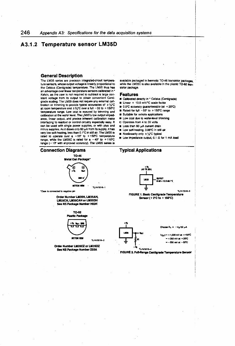
Univers
ity of
Cap
e Tow
n
246 Appendix A3: Specifications for the data acquisition systems
A3.1.2 T~~mperature sensor LM35D
General Description The LM35 series are precision integrated-circuit temperature sensors, whose output voltage is linearly proportional to the Celsius (Centigrade) temperature. The LM35 thus has an advantage over linear temperature sensors calibrated in • Kelvin, as the user is not required to subtract a large constant voltage from its output to obtain convenient Centigrade scaling. The LM35 does not require any external calibrabon or trimming to provide typical accuracies of ± Y."C · at room temperature and ± 31."C river a full - 55 to + 1 SO"C temi>erature range. Low cost is assured by trimming and calibration at the wafer level. The LM35's low output impedance, linear output, and precise inherent calibration make interfacing to readout or control circuitry especially easy. It can be used with single power supplies, or with plus and minus supplies. As it draws only 60 ,.A from its supply, it has very low self-heating, less than o.1•c in still air. The LM35 is rated to operate over a - 55" to + 1 SO"C temperature range, while the LM35C is rated for a - 40" to + 11 O'C range ( -1 O' with improved accuracy). The LM35 series is
Connection Diagrams TC>-46
Metal Can PllcUge"
•eu., is connecl8d to negative pin
TUH/5518-1
Order Number Ul35H, Ul35AH, Ul35CH, Ul35CAH or Ul35DH See NS PKkage Number H03H
IOTT1lll ¥EW TUH/5518-2
Order Number Ul35CZ or Ul35DZ SH NS P1lcUge Number Z03A
available packaged in hermetic T0-46 transistor packages, while the LM35C is also available in the plastic T0-92 tran. sistor package.
Features • Galibrated directly in • Celsius (Centigrade) • Linear + 10.0 mvrc scale factor • 0.5'C accuracy guaranteeable (at + 25'C) • Rated for full - 55' to + 1 SO"C range • Suitable for remote applicaoons • Low cost due to wafer-leilel trimming u Operates from 4 to 30 volts • Less than 60 ,.A current drain • Low self-heating, 0.08"C in still air • Nonlinearity only ± y."C typical • Low impedance output, 0.1 n for 1 mA load
Typical Applications
+Vt (4Y TO IDYI
I i ~= ... ,. TUH/5518-3
FIGURE 1. Balk: Centigrade Tempereture Sensor ( + 2'C to + 150'C)
.$r-.~ -Vt
TUH/551~
VOUT- +1,500 mV at +150'C
- +250 mV at +25'C - -550 mV at -55'C
. FIGURE 2. Full-R•nge Centlg'8Cle Tempeniture SeMor

Univers
ity of
Cap
e Tow
n
Section A3. 1: Transducers and data logger specification sheets
A3.1.3 LEM current probe LA 50-P
Definition-Principle The "LEM ~:odule LA 50-P" is a curr.;>nt iwn~or f<)r P.lec::.ronic measurin11 of c'.1rn:nts : DC. CA. H!Pl ... Pr<"., wit.h eli1Vlin:ic isolation between tl"1c prima1·y (h.i.eh \:u=nmt) 1:1m\ th<.' $t.'Cond11ry (el ectnmit:) cirt:uit. Batt"!d on th11 print:iple of .::nmpc.;n~at.io:1 a: :he rr.ag1:etic f i•?.l.d, the LE!-! ut-nUL'r~ supply a mo'Jasur.ing current pro;:-,orr.hine<l to the pr.ir.1nry c:urr~nt.
Electrical Data !lc•1•:lna l Cun· en t IH M1.~~.1 :qJT ; ~tL, t ~.i.nge
T''.::-n re; t io Measuring currt.>nts
D::-ift wit.h temperature
Line11rity Res pons c~ t i.mc? <.llf<.lt. accuraLely followed Test vol.t!lf,e
secondary circuit Ccnnection Int~rnal re~istente
Supply voltage Current <!rain
General Data ~:xc-!'t:~t.iun
Mounting
DimC!nsions Operating temperature Storage temperature "In-O~t· cign~l c~nce
· Particularity
SO A :·ms 0 to +/- 70 A (supply voltege + and - 15 V,
R. meas. • 100 oh~~) - : 1000 - noir.. 50 rnA for 50 A - max. 70 mA for 70 A +!- o.s % of IN at 25°C ~1:cL1i:!ing offset c:lir=er.t i;t I pr.irn. 2 o cr:ax. +/. n.:: ::-~\
of thP of f~At current bet.wefin O" and :o"c typic'1.1: +/- 0.3!i mA
n~x.: +/- 0.50 mA 0.1 % better than 1 us better than 50 A/us bi!tween primary and secoi~d«ry c:!rc:ui:-. z kV rms./50 H;/l mn.
en 3 pins, section 0.63 x 0.56 nan 90 ohm at 1o•c (internal voltage drop 4.5 V/50 A prirr.aryJ + and - 15 V (+/~ 5 %) 10 mA (no-load c:urr.imt) t Im (measuring cu:i·er.t)
insulated pla~tic injected case mounting on printed circuit by 3 pins hole size 0.9 mm see drawings overleaf - weight 2!i g
o•c to + 7occ - zj~c to + ~~·c
• to obtain R po~itiv11 meaGuring curre~t on terminal M, t.he .primary current has to flow in tht! dir!!c:ticn of the arrow on the LEM Module
minimum measuring rasistan~e 100 oh."!ls
247

Univers
ity of
Cap
e Tow
n
248 Appendix A3: Specifications for the data acquisition systems
A3.1.4 Loadcell UBG 10
.;.,. .. ,
' ... .... ,. . ·::
·' B
0
.7SPECIFICATIONS ;•' . if.:"'.
* :·~_ti~. MT~C OUTPU'f (NOMINAL) mVIV
., . TEMPEllJ~TURE EFFECT ON ,.RO . ,. . RATED OUTPUT/"C ;(/ .,. TEMPERATURE E'FECT ON .. RO './!;· ZERO SIGNALl"C
,~ . . COMBINEO ERROR: t·)· .. RO :·:! llNEARl1rY -t- HYSTERESIS
. -~ "·
REPEATA·BILITY "4RQ
~···. CREEP AFTER 20 MIN AT 23°C . .. RO ....... _
INPUT Rlo$1$TANCE ~,'lio n ~ · .... .. .OUTPUT Ae51STANCE a
·'• ... / INSULATION RESISTANCE MO AT60VOC . .. ...
1 ........
~ RECOMMENOEO -v ·EXCITATIO.N AC/OC
·;:,~<
;MAXIMUM v 1( ;!!~CITATION ~C/OC
. 'sAl'E'OViliRLOAD .. RO ~ . ' '
.• :.u~T\MATE OVEAl.OAD 'MIRO .. . ' :liREAKIN() LOAD .. RO
,CABLE m. ,•1;
~ J
,..___ ue-1
s
0,003
Q,003
0,05
o.02 0,03
350
350
1k
8
,, ..
120
1eQ
300
s
ALL DIMENSIONS IN mm
'• . .'. •,
'CAP. (kg) ·. ·;
5.: 10, 20
. .
M8 . ···.:·
..
. · ...
:',: ..
. · .. ·
·-..·:··.· .. ..::.··: .. . ·:·
......
from:
A e 6& 60
. ELECTRICAL
.CONNECTIONS
---· ·-- -- -- ": . 1 ·aH1,LO f . • ... .. J
9LUI! li•O
.· AGO· 51$ +
·YELL t.xc,to-o--_.
GA! Sog1i-;;.o----'
c -
17.~

Univers
ity of
Cap
e Tow
n
Section A3.1: Transducers and data logger specification sheets 249
A3.1.5 Optical switch TCST 2000
Package 1 Pack ,ge 2 Package 3 Package 4
Output
TCS
____ _J -r -r T I I
T variations
T = Transistor I S =Schmitt-Trigger
I Package variations ---- _J I 1 =no.tabs I 2 =two tabs
3 =tab Emitter-side _J 4 = tab Det£ctor-side
Aperture vc:riations -· ---
0 =without
1 = 1 mm (0.04")
2 = 0.5 mm 10.02")
3 = 0.25 mm (0.01 ")
.:xamplt1 res -..'
Transistor-------' output
Package with 2 tabs
0.25 mm Aperture (0.01")
L.
l I
J
T I
I ~---CTR variations
(see table)
---- Variation vf output level
u ,.-' '
l
0 = open collector inverted
1 = open collector non inverted
(only for Schmitt-Trigger output)
T~---- CTR= 2.5%
L ___ no advise
because tr~nsistor output
Slot width Aperture
·,
We have the facilities to provide your soecial custom design, included wires and connectors

Univers
ity of
Cap
e Tow
n
250 Appendix A3: Specifications for the data acquisition systems
A3.1.6 Fl'ow-captor Type 4113.30
1)1!''/ / t 1Y9~~v-cap or Compact Flow Meter A~catlon examplea: Type 4113.30
Electrlcal Data:
Voltage supply
Oulput eurrer'lt
24 v oc ' 4to20mA
Current co'.1~urnµlion m8x. 100 mA • ,,
(
fl Digital display on
001 PC-captor wilh two ·:;i additional •t!h"Y 7 . outputs. applicat:>le
·~ U2·-·'°""'"' I .
.\ - 3. Mass ttow control
I
I I
I I
Cont1011er
~ 2 and 3 ui111 ba combined
weber·
R<1sistive load 0-600 Ohm
Measurement range aCljustment: . The two potentrometers prolected by covering hubs, allow for th<1 zero balancing and the aCljustment of the measurtng rangt1 by means of a small screwdnver. A color Changing LED signalizes !low within the aujustecJ measuring rangl!I (green) or ovorflow (red).
Connection diagrnm 4·20 inA current output
Mechanical Daw:
Material Sensorhead
Ceramic KER 221
Housing
81ainless steel WN 4305 PPS-Polyphenytensuttid
Operating pressure max. 30 bar. attention 1 not applicable under vacuum condrt10ns
~--------------------------------Med I um temperature -10° c to +80° C ranga (14° F to 175u F) --------Ambient temp91atura • 10° C to +GO" C
(14° F 10 160° F)
Union fitting R 1 •t." SW 50 DIN 259 ISO :~28 ---------8 ect rica I connection 2 m moulded oilflex cable
Protection standard IP65
Weight plastic approx. 230 g. sfainless stHI approx. 410 g
Oimensions in mm
'
Tfi ~ l:i &61
i--eo
11-========Lr-~~
:::~~~:@::::;.tt,:_~ • • ~ - !
stainless steel 1<---~~1oe~~~---!
90 --:JI! 5@ -----1-~~- * PPS-Polyphenytensulfid
This now-captor is also available in 25 mm 0 housing. (Type 4111.30)
Sensonecnnik GmbH D-2201 Kollmar · Strohde1ch 32 · Telefon: O 41281591 · Telex:. 218 326

Univers
ity of
Cap
e Tow
n
Section A3.1: Transducers and data logger specification sheets 251
A3.1.7 PSM water meter Size 3 Technical Specifications
Classification Size 3 Size 5 Size 7
Nominal Bore mm 15 20 25 32
PERFORMANCE
Starts to register at about t/h 4 4 6 14
Minimum accurate registration ±2% t/h 24 24 32 68
Flows at 30 kPa pressure drop kt/h 2 3 4,1 5,8
Flows at 100 kPa pressure drop kt/h 3,7 5.6 7,5 11
Maximum recommended continuous flow kt/h 2.8 3 4,6 6,8
Test pressure MPa 2 2 2 2
Maximum water temperature 'C 50 50 50 50
Counter resets to zero at kt 9999 9999 99999 99999
The group of white numbers in the counter (register) represent kilolitres and are used for periodic meter reading. The orange numbers represent litres and are intended to be used when checking the meter accuracy against a calibrated measure.
NET MASS
Meter only
Meter with connectors
DIMENSIONS
Length over body A
B
Length over connectors c
. Meter body screwed ISO·R7 thread
Connectors screwed ISO-R7 thread
MATERIALS
Body - brass SABS 200 1972 Code 9A.
Chamber - graphited styrene
Counter - diakon
Number wheels - delrin
Gear wheels - nylon
Spindles - nickel
kg
kg
mm
mm
mm
mm
mm
The PSM, designed for the measurement of ·potable water. has a specially developed thermoplastic work-_ ing chamber to ensure an exceptionally long working life. It is also highly resistant to chemically aggressive water whilst still retaining its high accuracy and reliability.
Standard Features
Semi-positive rotary piston of latest design which commences to register at extremely low flows and is accurate within plus or minus 2% throughout a wide range.
Counters and working chambers interchangeable between 1 5 mm and 20 mm meters.
1.2
114
44
200
20
15
1,3
1,7
165
44
267
25
20
.. ... z ....
"' ;;; ... w
"' > !
c
Optional Features
Disc-type non-return, valve.
2.4 3,6
3 4.6
198 198
57 60
311 327
32 40
25 32
Normally supplied with connectors for iron pipe comprising union nuts and tailpieces screwed BSP.
Connectors for copper pipe by means of flared-type reducing pillar cock adaptor can also be supplied.
Approved in terms of Section 21 of the Trade Metrology Act and Regulations.

Univers
ity of
Cap
e Tow
n
252 Appendix A3: Specifications for the data acquisition systems
A3.1.8 P1ressure transmitter Model 891.14.525
Pressure Transmitter· Model 891.14.525
Piezoresistive FEATURES
Pressure transmitter with piezoresistive sensor and temperature compensation. Stainless steel body with padded electronics
Output signal rising proportional with rising pressure applied
STANDARD FEATURES
Wetted parts of stainless steel 1.4571
Body of stainless steel
Pressure connection G •nA seating per DIN 16288
Electric outlet with L-plug per DIN 43650
Internal transmitting liquid silicon oil
Gauge pressure measurement
Output signal 4 ... 20 mA 2-wire system
Application - Measurement of positive and
negative pressure - of liquid and gaseous media - in fluid power and
pneumatic systems process plant and machine control General pressure instrumentation
Accuracy 0.5%
RANGES
0 ... 400 mbar 0 ... 600 mbar 0... 1 bar 0... 1,6 bar 0... 2.5bar
0 ... 4 bar 0 ... 6 bar 0 ... 10 bar 0 ... 16 bar 0 ... 25 bar
Other pressure ranges feasible
OPTIONAL EXTRAS
Other materials upon reQuest, see also Wl_KA S.A.P.-System
Other connections feasible
Outlet 1.5 m shielded cable Outlet 5-pin jack
Other liquids upon request
Absolute pressure measurement
3-wire system 0 ... 20 mA 0 ... 5V 0 .•. 10V

Univers
ity of
Cap
e Tow
n
MS-256 Messwerterfassungssystem
Da• System MS256 iat ein Mikroproze••or ge•teuertea Me~ayatem, d•• fQr den Einsatz in der Langzeitmeastechnik entwickelt wurde. Es besteht aus modularen Romponenten, die autonom vor Ort Me~daten erfa•••n konnen.
ms-256 Messwerterfassung mil System
PROZt:SS-CROSS£N
.Digital
8 Ein90n9e: m oder potentiotfreier Kontokt Ereignis oder Betriebs.zait
Analog
8 [;t,9on9c: 0 ... 10 Volt oder 0 ... 20 mA
Betriabsort: Mittelwert. Min.-, M~ximolwert
-· .......
;::::-tdl
In der Abbildung sind die Romponenten einea einzelnen Messkopfes dargeatellt. Jeder Meaakopf iat mit einem Netzteil und einem Akku-Puffer auageruatet. Ein Messbetrieb uber 24 Stunden bei ausfallender Ver•orgungsspannung kann garantiert werden. Der Datenapeicher, die Ronfiguration und die laufende Zeit/Datum, werden uber eine Lithiumbatterie fur 5 Jahre versorgt.
)
)
)
Analog
Jeder MePkopf des Systems MS256 hat acht analoge Eingangskanile fQr Strom- oder Spannungameaaung. Die M•Prate de• A/D-Wendlers betrigt 700 Mesaungen/Sekunde/Ranal. Alle Me~werte eines Abapeicher Intervalls konnen zu einem Mittelwert verdichtet werden. Durch dieaea Verfahren wird eine Aufloaung von 16 Bit er~ielt.
Jeder Analogeingeng~kann wahlweise eine der folgenden Aktivierungen einnehmen:
Mittelwert Mittelwert ' Minimum Hittelwert ' Maximum Mittelwert ' Minimum ' Maximum Momentanwert
(28yte) !4Bytel (48ytel (6Byte l (2Byte)
Der in Rlammern.angegebene Wert zeigt den benotigten Speicherbedarf pro Intervall und Renal. Eine gemischte Belegung aller Ranile iat jederzeit moglich.
Digital
Die acht digitalen Eingangskanile warden fur die Messung von Betriebazeiten oder Ereigniaaen eing•••tzt. Jeder Digitaleingang kann dabei wia folgt aktiviert warden:
Betriebszeit Ereignia
(2Bytel (2Bytel
Auch hier beziehen sich die Werte in den Rlammern auf den Speicherplatzbedarf pro Intervall und Renal. Die digitalen Einginge sind fur den Anachlu~ von TTL-Signalen oder nicht entprellten Einzelschaltkontakten eingerichtet. Werden Zihlerstinde mit mehr ala 16-Bit (65535) benotigt, so konnen alle Digitaleinginge z.8. zu 32-Bit Zihlern kaskadiert werden. Eine Anzeige des Schaltzustandes ist jederzeit moglich (Hmoffen I L•geschlossenl. Die Entprellung der Einginge kann auf 3Hz .•• 3RHz ertolgen. Die maximale Zihlfrequenz betrigt 2 MHz.
)> w . ~
Co c I» ,... I»
r-0 cc cc Cl) ft) <b ...
~ 3: ::;, en ):.
I ~ N ~ en
en ;i Qj ::;, (I)
2-~ c;i Ill ::;, ll.
IS-ii)
Ci ~ ~
~ Q. ~ ~ 5· ::;,
~ <b
~
I\) 01 (,.)

Univers
ity of
Cap
e Tow
n
254 Appendix A3: Specifications for the data acquisition systems
A3.2 Interface circuits and description
The purpose of the interface is to process the signals from the transducers to meet the signal input requirements of the data acquisition system (DAS). As the DAS has an instantaneous sampling frequency of 1 Hz, signals from the transducers should be processed to near DC quantities. Additionally the signals to the logger must be limited to the zero to 1 OV range.
This section discusses the design of the interface signal conditioning circuits, their transfer functions and their settling time as for the parameters listed in Table 5.1 (except the inverter current, frequency, voltage and power - section A3.3). Additional information is supplied where necessary (like present settings, trimming procedure hints and where applicable possible improvements).
Horowitz and Hill (1989) was used as the main reference for the design of the electronic circuitry.
The settling time (t5 ) is the time that it takes the output to settle to within 1 % of its final value after a change in input signal. It is calculated as follows:
V(t) = vfinal x (1 - e·t/RC)
0.99 : 1 - e·t!RC
When a few RC time co11stants aceJin a circuit then the overall settling time is calculated as follows:
The settling time is important as it indicates the time required for DAS to settle to steady state values after a change of input to the system under test. The settling time for instance should guide the logging interval. Under dynamic conditions the parameters can be brought to the same time instance with the use of software filters. This is not required here since the main emphasis is on steady state operation. Dynamic conditions are only_ investigated in terms of system stability.
App. A3.4 contains the introductory data sheet for each IC mentioned in this section.
The circuit diagrams use the following conventions: The transducers are shown on the left. Each IC is numbered with ICx where 'x' is a particular number. Where appropriate the output of an IC is named with Sx (signal number). The gain is usually stated above the component with Gx. Px are multi-turn potentiometers. A resistor value like 12k + 5k- means a fixed resistor of 12k!l in series with a 5k!l potentiometer. Ri is an input

Univers
ity of
Cap
e Tow
n
Section A3.2: Interface circuits and description 255
resistor to an op-amp and Rf is a feedback resistor of an op-amp. The roll-off and cutoff frequency refer to the -3dB point. RC is the time-constant and is referred to as 't. v out is the output signal which is sent to the data logger.
A3.2.1 lrradiance
The Ll-COR pyranometer requires a termination resistor whose value will result in a voltage of less than 10mV at 1000W/m2
. A resistor value that is too large can result in a non-linear response. A 1470 resistor or less is recommended in the specifications.
LI-<:OR Pw,.•nometer"'
t•mP•r'atur"'• sensor
G POR
2k2
330nf"
68k 20k
FIGURE A3.1 Circuit diagram of the irradiance and temperature parameters
It was decided to choose a trans-impedance op-amp configuration as shown in Figure A3.1. This results in an input impedance of 0.270 meaning the Ll-COR is virtually operating at short-circuit.
R, Zin= --
( 1 + A)
where A is the open loop gain of the op-amp (here 11 OdB).
The Ll-Cor is calibrated at 94µA/1 OOOW/m2 . A maximum irradiance level of 1250W/m2
will result in a photocurrent of 117.SµA. A feedback resistor of 85k0 will set the fullscale signal to 1 OV. The input bias current of the LM324 is typically 45nA and the input offset voltage is typically 2mV. At 200W/m2 (which is the lowest value of interest) the Ll-COR generates a photocurrent of 19µA and the op-amp output is about 1.6V. Neither the bias current nor the offset voltage will cause a serious error (0.24% and

Univers
ity of
Cap
e Tow
n
256 Appendix A3: Specifications for the data acquisition systems
0.01 % resp1ectively).
The roll-off frequency of the LPF is 5. ?Hz with a settling time of 130msec. The output is adjusted with P1•
The transfer function is:
A3.2.2 Temperature
The LM35D produces an output of 1 OmVl°C. It is amplified by ten with a non-inverting op-amp configuration (Figure A3.1 ). The gain is set with P2 and P3 for the ambient and module temperature circuit respectively.
The 2k2!l resistor is added to decouple the capacitive load of the long cable (about 1 Om) else a high frequency ripple occurs on the output of the LM35D. The f_3de point of the LPF is at 0.9Hz with ~ being 0.77sec.
The transfer function is:
tamb/mod = G2 X V out [°C]
A3.2.3 Arrray voltage
The array voltage is processed by IC1 and IC2 in Figure A3.2. IC1 is a differential opamp which has a gain of 1/30. Care has been taken to match the resistors although the amount of common-mode signal is small. The inverting op-amp configuration (IC2) is used to fine-tune ~he gain to 1/30 with P1 and to roll off the signal at 0.48Hz with ts = 1.52sec.
The L T1097 is used for both op-amp's. It has a very low input offset voltage (SOµV max) and bias current (250pA max). The array voltage is usually fixed at either 90V or 180V and is therefore scaled to 3V or 6V in Figure A3.2 respectively. The offsets are consequently negligible and no trimming was required.
Transfer Function:

Univers
ity of
Cap
e Tow
n
Section A3.2: Interface circuits and description 257
A3.2.4 Array current
The voltage drop across the shunt is fed into a differential op-amp (IC3) with a gain of 4.7. The output is sent into a two pole Butterworth LPF with f.3de = 0.48Hz and ts = 1. 78sec which removes the ripple caused by the switching of the inverter or converter. The output of IC4 is sent to two non-inverting op-amps with different gain. The one branch has an overall gain of ten and is used for the array current when the array is in the parallel configuration (higher array current: Miltek and ML T system). The other branch is used when the array is in the series configuration (Solvo system). Only the gain of IC6 can be adjusted. The output of IC5 has to have a calibration factor.
Arr aw
e e V .,.,.
I .,.,.
Inverter
Or'
10k
10k
!Gl = 1230.081
!G3 = 4. 71
47k
33k 100k
9Sk
!<:4 = 1.$8 I
3k3
!<: = 1230 I
3k3
. ,,. 10k
ror parallel arr aw
FIGURE A3.2 Circuit diagram of array voltage and array current parameter
The IC3 op-amp uses an LM627 which has a gain-bandwidth product in excess of 10MHz and a negligible input offset voltage. It does however have an input offset current of 50nAmax· This becomes problematic if the op-amp sees a large input resistance on one op-amp input as it will result in a voltage drop across the resistor. A LM627 was used for IC4 but exactly that problem occurred. Instead of adding a resistor of similar value to the other input (to reduce the offset current) a LF351 which is also a wide-band op-amp was used. It does not have the precision of the LM627 but its input bias current is a factor 1000 lower. The offset voltage in the array current measurement branch for the parallel array configuration cannot be trimmed to zero as no trimming potentiometers were added. However the maximum recorded offset was 0.5mV. The series array current measurement can be trimmed to zero with potentiometer P 2•
Transfer Function:
larr = V out + (Rshunl X Gioia!) [A)

Univers
ity of
Cap
e Tow
n
258 Appendix A3: Specifications for the data acquisition systems
A3.2.5 Converter voltage
The converter voltage (Figure A3.3) has in principle the same circuit as the array voltage except that it uses a two pole Chebychev LPF in an inverting op-amp configuration. The cutoff frequency is at 0.48Hz and ts is 1.76sec.
Convert•r
o. 1 <~
<'
v
I con
!(;I = 0.047
24k
SlOk
510k
!G3 = $.61
56k
!G2 = 1 77 I
479k
lOOOnF"
!G = 12121
!G4 : LSI
390k 390k
9k05
11k35
FIGURE A3.3 Circuit diagram for the converter voltage and converter current parameter
No provision has been added to trim the input offset voltage zero. The maximum recorded offset voltage was -3.4mV.
The transfer function is:
A3.2.6 Cc>nverter current
The voltage drop across the shunt is fed into a differential amplifier with a gain of 5.6 (Figure A3.~~). The LPF is a Chebychev type filter with a cutoff frequency at 0.53Hz and a ts of 11.6sec. The overall gain is set to ten.
Note that the shunt is in the positive line to the motor. During measurements on the Miltek system the positive lead is tied to ground and the array current is also

Univers
ity of
Cap
e Tow
n
Section A3.2: Interface circuits and description 259
measured in the positive lead to the converter (the converter switches the negative lead to the motor, see Figure 3.2 in main text).
The transfer function is:
A3.2.7 Motor torque
The circuit for the torque measurement is shown in Figure A3.4. The sensitivity of the loadcell is 3mVN. With a 10V0 c excitation this will result in a 30mV full-scale signal riding on about 5V. The common-mode rejection requirements of the op-amp has to be 90dB if an error of 0.5% is tolerated (20 log (5000/(0.005x30]). The L T1097 has a CMRR of minimum 115dB and maintains it above 90dB for frequencies up to 5kHz. The resistors have been well matched. IC2 provides for scaling, zero adjust and offset adjust. Its output is instantaneous and can be used for a fast sampling device. IC3 is a unity gain amplifier with a two pole Sallen and Key LPF which has a 1-ads point at 0.25Hz with t being equal to 640msec. This is a long time-constant and to reach 1 % of its final value (from a step input) requires 4.6 x t seconds which is 2.9sec.
!G2 = 40.8 I
L..oadc•ll UBQ 330k
SlOk
T mot 10k
R = 3SO
Optical Switch TCS T 2000
+ v
5 soo mot
:-·-···· .............. ·····--:
I. ~ ~ . I i E 0 ! ~--···· ·············· ...... .;
lOk lOOk
lOOk 390k
-1 v
f 1ip-f'1 OP 4013
lk 11'1
'---'V'lOv"-k ---l'" l oc:k Qll---------41
TTL
lOk
to pul 1-up re•i•tOr" in d•t• 109~.,..
FIGURE A3.4 Circuit diagram for the motor torque and motor speed parameters
The motor torque is calculated by multiplying the force F on an arm of length L. The gain was adjusted so that 1 kg would result in 2V output. Consequently the transfer function is:

Univers
ity of
Cap
e Tow
n
260 Appendix A3: Specifications for the data acquisition systems
A3.2.8 Motor speed
Tmot =FxL =mass x g x 0.25m = 2.45 x mass
- = 1.225 V0 u1 [N.m]
An optical switch is used to count the revolutions per log-interval (Figure A3.4). A disc which is mounted on the motor pulley has eight flags (or in some cases two or three flags) to interrupt the light barrier. At very high motor speeds (larger than 131 Orpm) the interrupt1ion frequency of the light barrier exceeds 175Hz (data logger maximum). A divide by two circuit is therefore added. The flip-flop halves the frequency from the optical switch.
The output of the flip-flop drives the base of a tra11sistor. The open collector is fed into the data logger where it is pulled up to 5V via a 5k6n resistor when no base signal is present. ·
The transfer function below uses the variable count C as the one recorded by the data logger. The number of flags F and the log-interval i relate C to the motor speed in units of rpm.
The transfer function is:
Smot = 2 x C + (T x i) [rev/min]
A3.2.9 Fl1owrate
The flow-captor is directly connected to the data logger as can be seen in Figure A3.5. The flow-captor allows for zero and span adjust on the device itself. The flowrate can be calculated from the flow speed but it is far more accurate to calibrate the flowrate with a bucket of known volume.
A3.2.10 Static and pressure head
The pressure transmitter is directly connected to the data logger. Due to its large pressure range it is not the most suitable to measure a pressure of half a meter.
Transfer Function:
Pr = 2 x (Vout - 2) [bar]
•

Univers
ity of
Cap
e Tow
n
Section A3.2: Interface circuits and description 261
The depth probe is used to measure the water level in the borehole. It has markings on the cable indicating the depth.
,..•sist."nc• ~ of' water
1
Q Pr 4-20mA
H. ____ / /.---------.--.--.----.--1
Cabl• i• 100m long
____ / /.----'VV'---,.--....---1
lOOk
4-20mA
· FIGURE A3.5 Circuit diagram for the flowrate, pressure and static head parameter
A FET is used to activate an LED or a speaker when the probe makes contact with the water. The resistance of the water provides a gate drive signal to the FET.
A3.2.11 Power Supply
2N3773
Ll1781S
VI S VO O. lu 6
l 330u
l
120
r ·FIGURE A3.6 Circuit diagram of the interface power supply

Univers
ity of
Cap
e Tow
n
262 Appendix A3: Specifications for the data acquisition systems
The power supply must provide power to the transducers and the interface. Most transducers only require a single voltage supply (loadcell = 1 OV; flow-captor = 24V). As some signals can be very small (for example GPoA in the morning and afternoon) it is quite appropriate to use a split supply to avoid non-linearities.
Power is obtained from two batteries in series, that is 24V. That supplies the flow captor, the pressure transmitter and the depth probe directly. The battery voltage is fed to a active zener clamp which reduces the voltage to 20V plus a diode drop. This was done because a few regulators were having to dissipate a substantial amount of power. The 20V is fed to an adjustable regulator (set to 10V for the loadcell and the optical switch) and to a 1 SV regulator (LM7815). Minus 1 SV are generated from the +1 SV by mE!ans of voltage converters (Si7661 ). Four of these were used in order to provide the current that was required. The negative voltage is regulated with an adjustable regulator to generate about -11V.
A3.3 Power meter circuits and description
The power meter is a stand-alone unit which converts the current and the voltage to rms DC quantities. The inverter frequency is derived from the current and the active power is derived from the instantaneous multiplication of the current and the voltage. The device has its own power supply and requires a 24V power source. Figure 3. 7 shows the g:eneral layout of the power meter with respect to circuit distribution on the printed circuit boards (PCB). I[;.::: mmmmm m -- m m mmmm m ~::;~~- mmm m m mm mmm mm m I
: :
1·······~~~~~··:~~~~-~·····-·1 I i /- 1SY & +/- SY i L p F i
i FlCB 4 ! PCB 1 ! :--··'Pc:·8·····2···············'······ ···························································································r··;;·c:8····3·················································1
Floatin9 po~•r SUPPlW
+/-lSV & +/- SV
!~ ~! l ................. ············· ························ ................................................................. ········ .......... --~---·· ..... ········. ·········· ...................... ··············· ..... j
FIGURE A3.7 Block-diagram of the PCB layout of the power meter

Univers
ity of
Cap
e Tow
n
Section A3.3: Power meter circuits and description 263
The distribution is as follows:
• PCB1 contains the line current and the frequency processing circuitry.
• PCB2 consists of the voltage and the multiplication circuitry. Signals on this PCB are floating with respect to signal ground.
• PCB3 contains the circuitry that couples the floating voltage and power reference signals to the signal ground side.
• PCB4 contains the power supply for the power meter.
What follows is an explanation of the circuitry with additional information on the choice of components, the transfer functions and the settling time of the parameters. If applicable additional information is supplied.
Refer to the introductory paragraphs of section A3.2 for information on conventions.
A3.3.1 Inverter current
The LEM module (bandwidth: DC to 1 OOkHz) generates a proportional current (1 :1000) for the primary current and returns it through its ground lead as shown in Figure A3.8. A measurement resistor (Rm) converts this current to a voltage. Accuracy is increased by increasing the number of turns through the LEM provided one does not exceed 50 A (that is number of loops times line current ~ 50) and provided there is more than 60mA available from the power supply to drive the LEM. The loops through the LEM and the size of the measurement resistor (not less than 1000) must be chosen such that the maximum rms voltage at S1 is 2V.
IC 1 is a unity gain inverting op-amp, the L T1097 (low input offset voltage, 700kHz bandwidth). The non-inverting input can be tuned at P6 to null the LEM offset current (due to drift caused by temperature variations) of up to 350µA and maximum 500µA. This current would be converted to a voltage at the measurement resistor and would result in an undesired voltage offset. The output of IC1 is distributed for multiplication, RMS to DC conversion and frequency measurement.
IC2 (L T1097) is configured as a voltage follower and acts as a buffer into the RMS to DC converter as it has a fairly low input impedance.
IC3 is an RMS to DC converter, the AD637 (high accuracy, maximum nonlinearity at 2Vrms is 0.04%, 3d8 bandwidth at 2Vrms is 8MHz). Depending on the frequency range of the signal, an averaging capacitor is chosen. The fundamental frequency varies from 6 to 85 Hz. Highest accuracy is required in the 40Hz to 85Hz range. When choosing an averaging capacitor (Kitchin & Counts 1986) there is a trade-off between the averaging error and settling time. Presently a 680nF averaging capacitor (Cav) has been selected. All the higher harmonics that are part of the current spectrum will be converted with negligible DC error. The peak ripple (or AC error) can be reduced by

Univers
ity of
Cap
e Tow
n
264 Appendix A3: Specifications for the data acquisition systems ·
post filterin~r. A one pole filter at the output has been selected with C2 equal to 2.2µF and R equal to 24k!1. Error and settling time can be read off from a graph in Kitchin and Counts (1986: Figure 24). The scale factor of the AD637 can be trimmed but is internally laser trimmed to 2Vrms· There is consequently no need for scale factor adjustment in this application as the signal processing pre-AD637 has been designed for 2Vrms·ma1ximum input signal. The're is however provision for this potentiometer. P
2 (50k) trims the output offset voltage to zero.
G. ...
~ 10k
Rm 100
7Sk+20k-
22K
390k
SOk
lOk
FIGURE A3.8 Circuit diagram of the inverter current and the frequency parameter
IC4 (L T109?) is an active two pole Butterworth LPF (Gain= 1.57, /_3de = 0.604Hz, i: = v!(RC2+RC2
) = 372ms) to smooth any ripple that may remain on the signal from the AD637.
IC5 is a gain stage which is adjusted with P4 • .Que to the low offset op-amp, P3 has been removed (Offset trimming is provided on the PCB but is only compatible to LF351 pin configurations {Pin 1 & 5 for offset trim}).
The transfer function is as follows:
where V out is the output signal at S6 , N are the number of turns through the LEM probe, Rm is the measurement resistor that converts the current out of the LEM probe and Gx are the respective gain stages.

Univers
ity of
Cap
e Tow
n
Section A3.3: Power meter circuits and description 265
The settling time (t5 ) has to be calculated for the whole lline circuit. Delays occur only at IC3 and IC4.
ts = 4.6 x J ( 0.68 x 0.025) 2 + ( 2.2 x 0.025) 2 + 2 x ( 0.47 * 0.56) 2 = 1. 73 sec
where the first value in brackets is always the capacitor in µF and the second value is the resistor in M.O. The AD637 has an internal 1 k.O resistor in series with the 24k.O external resistor.
A3.3.2 Inverter frequency
The circuit which processes the fundamental frequency is also shown in Figure A3.8. IC6 (MF6-100) is a six pole switched capacitor lowpass filter with two on-board opamps where one is used to scale the voltage to between 4V to 5V using P 5. The cutoff frequency is set to 105Hz (clock frequency= 1/1.69RC = 10.5kHz) with an RC network on the Schmitt trigger input to retrieve the fundamental frequency.
IC? is a comparator for zero-crossing detection. The resulting square wave (OV or 5V) has the same frequency as the fundamental frequency and can be logged by a digital channel that has a counter. The threshold voltage Vthresh is set to 0.45V (that is Vthresh = [Ri I [Ri + Rf ]]x5V = [1 Ok/[1Ok+100k]]x5V = 0.45V). Hysteresis is determined by the resistor divider ratio which is one to eleven. It can be increased by decreasing the size of the feedback resistor. This could be required in cases where the switching frequency has a low value since the harmonics will then appear closer to the fundamental frequency resulting in a ripple on the current waveform which can cause multiple triggering. However it can be expected that the six pole filter will remove those harmonics.
The transfer function is:
f fund = count + log-interval [Hz]
A3.3.3 Inverter voltage
The inverter voltage has to be isolated from the signal ground since it does not have a neutral which is or could be on the same signal level. Even a fictitious neutral (as created by a star termination of three resistors) will have a fluctuating neutral with respect to signal ground. Isolation also provides a form of protection for the circuitry on the reference side should a fault occur on the floating side.
The line-to-neutral voltage (V LN) is obtained by star termination of three 1 OOk.Q precision resistors. The circuit is displayed in Figure A3.9. The voltage is reduced by

Univers
ity of
Cap
e Tow
n
266 Appendix A3: Specifications for the data acquisition systems
a ratio of 1: 150 by means of the differential amplifier IC8 (LM627, 14MHz gainbandwidth product, low offset voltage, high CMRR and PSRR). IC9 is an inverting opamp set to unity gain, but can be scaled with P5 for desired peak value.
·······································-·
SOk
100k
100k h
INsuiral >--~
+ s
i G ¥, !A0202
!Pha•« 3>--~
l~I -
x x + w Sl 2 1 ~ 1
Sl
4.7
IZISQ I
lk Ill:]
1~21:1 = I I !SD
~ 1SO
3k
4k7
-vs C/S
~ +VS O/S
1Sk NC .;NO l!m
G ... IN NC
Ll1627 <En:>
,FIGURE A3.9 Circuit diagram of the floating inverter voltage and the floating active power parameters
S9 is distributed to the multiplier and to the RMS to DC converter. IC 1 O is a voltage follower wh~ch acts as a buffer to the AD637. Bandwidth is preserved up to and including th1e RMS to DC converter. The multiplier should not receive a differential signal larger than ±1 V. The differential resistance Rdiff must be chosen such that the peak output voltage at S8 is 1V (or scale with P5) rather than 1Vrms to avoid clipping at the multiplier.
IC11 is the AD637. It has the same configuration as the AD637 for the inverter line current.
A two pole Sallen and Key filter (IC12) reduces the ripple that may still be on the output of th1e RMS to DC converter. Its cutoff frequency is at 4.5Hz.
Power to thE! isolated circuitry is provided by means of DC to DC converters which are isolated to ~SOOV. They receive 12V and generate ±SV and ±1 SV to supply all the circuitry shown in Figure A3.8 (the AD834 requires ±SV and the AD202 requires +15V). The floating ground differs from the signal ground reference as can be seen at the AD202 (IC 1) where the input ground symbol (IC1 left) designates the signal

Univers
ity of
Cap
e Tow
n
Section A3.3: Power meter circuits and description 267
ground reference and the output ground symbol (IC1 right) designates the floating ground.
The floating signal is coupled across with the AD202 (IC 13) in Figure A3.10. A LPF at the output of the AD202 reduces the 25kHz ripple as introduced by the AD202. The non-inverting op-amp (IC14) is the final gain stage where the offset voltage of the AD637, the AD202 and the LF351 can be trimmed to zero with P3 . The input offset voltage of the AD202 can be as large as 1 OmV. It therefore makes sense to use a low-cost op-amp whose trimming range is large enough to null all the offsets. The gain of the LF351 can be adjusted with P4 .
·············································································~ ~
F" - + ~ ~
N , I
F" - + ~ ~
N , I
+ s l -=-
G V +
s s - +
33k
220~
!Gt = 63.4 I
LF"3S1 <lil>
LF"3S1
~
10k
SlOk
2k+lok-
FIGURE A3.10 Circuit diagram of the inverter voltage and active power parameters referenced to signal ground
The transfer- function for the line-to-line voltage is:
where Vout is the output signal at S14 and Gx are the respective gains in Figure A3.8 and A3.9 which form part of the VLL circuit.

Univers
ity of
Cap
e Tow
n
268 Appendix A3: Specifications for the data acquisition systems
The settling time is:
t8 = 4.6 x J ( 0.68 x 0.025) 2 + ( 2.2 x 0.025) 2 + 2 x ( 0.47 x 0.075) 2 = 0.35 sec
where the first value in brackets is always the capacitor in µF and the second value is the resistor in Mn.
The reason for this comparatively short settling time has purely logistic reasons. Since a lot of alterations took place at the test site the case occurred where a particular component was not available. In this case no op-amp with a low bias current was available and therefore the input resistors chosen had to be smaller to avoid significant voltage drops at the input of the op-amp. Larger capacitors were also not available.
A3.3.4 Inverter active power
The circuits for P active are shown in Figure A3.9 and A3.10. The current reference signal (11ineimu1tiplier) from Figure A3.8 is coupled across to the floating side with the isolator AD202 (IC1, 2kHz bandwidth, output resistance = 7k0) for multiplication purposes. The gain of the isolator is 1 /(2 x-../2) to reduce signal magnitude to ±1 V PP (the current is a sine-wave and square-root of 2 is therefore valid). The AD202 receives its power from the floating power supply.
Due to a relatively large bias current (typically 45µA) from the multiplier AD834 and a large output resistance of the AD202 (about 7k0) the output signal from the AD202 has to be buffered. The L T1097 (IC2) acts as a buffer and therefore avoids voltage offsets due to bias current. The magnitude of the input offset current of the AD834 is not mentioned in the data sheet.
The AD834 (IC3) is a 500MHz wide-band four-quadrant multiplier. This is far in excess of the bandwidth required but was the best option available at the time of design. The multiplier has a current output which is converted to a voltage and then amplified by IC4 to produce an output of ±1 V FS for ±1 V into the multiplier inputs (this circuit has been copied from the specifications sheet of the AD834). A potentiometer P3 (1000) has been added to one of the potential divider legs in the circuit to trim the op-amp output to ze~ro.
IC5 (LM627) is configured as a voltage follower. In addition, the input is configured as a two pole Sallen & Key with /_3de = 0.6Hz and t = 372msec.
Isolated power is supplied to the circuit as explained in the subsection on the inverter voltage above.
The floating power signal is coupled across to the signal ground reference in the AD202 (as shown in Figure A3.10). The circuit for the rms voltage and the active power are virtually identical. The gains of the LF351 's are different though. The input

Univers
ity of
Cap
e Tow
n
Section A3.3: Power meter circuits and description 269
offset voltage can be trimmed to zero as explained before.
The transfer function is as follows:
where Vout is the signal at S7, N is the number of turns through the LEM probe, Rm is the magnitude of the measurement resistor of the LEM, and Gx are the respective gains in Figure A3.9 and A3.1 o.
The settling time for the active power circuitry is:
t8 = 4.6 x ../ 2 x ( 0.48 x 0.56 ) 2 = 1. 71 sec .
A few alterations can be suggested.
• Replace the AD202 with a higher bandwidth isolator to couple across currents with harmonic content in excess of 2kHz.
• Replace the AD834 with the AD734. It has a full-power bandwidth of 1 OM Hz (which is more appropriate), a full-scale differential input range of ±12.5V, a lower power consumption, a wide power supply range. It is very accurate and generally more versatile.
• Move the DC to DC converters off the printed circuit board that it now shares with the circuitry in Figure A3.9. It may have caused interference with the rms voltage signal due to poor layout. Rather have it on a PCB by itself.

Univers
ity of
Cap
e Tow
n
270 Appendix A3: Specifications for the data acquisition systems
A3.3.5 Power Supply
The input voltage to the power supply can be between 24V to 28V (Figure A3.11 ). The transistor circuitry at the input 'regulates' the voltage to about 20V. This circuit is implemented to reduce the strain on the other regulators which were getting excessively hot. Power dissipation was sometimes in the order of 12V x 120mA = 1.44 Watt. A high watt resistor (390) was inserted in line before the LM7812 which supplies the DC to DC converters as it was still getting too hot.
2N3773 39 Ohm
!HE 220
1 1
lul
;f lOu
SI7661
• ! 10u
;f lOu
SI7661
YI ~ YO
L'179LOS
FIGURE A3.11 Circuit diagram of the power meter power supply . .
Minus 20V is generated from the Si7661 voitage inverters. Their output is regulated to -15V.
The power supply could be improved by increasing the negative supply current capabilities so that the LEM module can generate ±50mA at full-scale signal on the primary sidet. Currently the power supply is limiting the LEM current probe to 20mA on the negativE! supply rail. This is therefore a loss in resolution since the turns through the LEM can not be increased until it reaches 50mA on the secondary side.

Univers
ity of
Cap
e Tow
n
Section A3.4: Data sheets for electronic components 271
A3.4 Data sheets for electronic components
The data sheets (the first page only) for the components are listed in the sequence in which they occur in the previous two sections. -
Op-amp LM324
General Description The LM 124 series consists of four independent, high gain, internally frequency compensated operational amplifiers which were designed specifically to operate from a single power supply over a wide range of voltages. Operation from split power supplies is also possible and the low power supply current drain is independent of the magnitude of the power supply voltage.
Application areas include transducer amplifiers, DC gain blocks and all the conventional op amp circuits which now can be more easily implemented in single power supply systems. For example, the LM124 series can be directly operated off of the standard + 5 Voc, power supply voltage which is used in digital systems and will easily provide the required interface electronics without requiring the additional ± 15 Voc, power supplies.
Unique Characteristics • In the linear mode the inpu1 common-mode voltage
range includes ground and the ou1pu1 voltage can also ·swing to ground, even though operated from only a single power' supply voltage.
• The unity gain cross frequency is temperature compensated.
• The input bias current is also temperature compensated.
Advantages • Eliminates need for dual supplies • Four internally compensated op amps in a single
package • Allows directly sensing near GND and Vour also goes
toGND • Compatible with all forms of logic • Power drain suitable for battery operation
Features • Internally frequency compensated for unity gain
• Large DC voltage gain 100 dB • Wide bandwidth (unity gain) 1 MHz
(temperature compensated)
• Wide power supply range: Single supply 3 Voc, to 32 Voc, or dual supplies ± 1.5 Voc, to ± 16 Voc,
• Very low supply current drain (700 ~Hssentially independent of supply voltage
• Low input biasing current 45 nAoc, (temperature compensated)
• Low inpu1 offset voltage 2 mVoc, and offset current 5 nAoc,
-• Input common-mode voltage range includes ground • Differential inpu1 voltage range equal to the po'Wer sup
ply voltage • Large Ou1pu1 voltage swing o Voc, to V + - 1.5 Voe
Low power, precision op-amp LT1097
FEATURES • Offset Voltage SOpV Max • Offset Voltage Drift 1.0pV/°C Max • Bias Current 250pA Max • Offset Current 250pA Max • Bias and Offset Current Drift 4pA/°C Max • Supply Current 560,J\ Max • 0.1Hz to 10Hz Noise 0.5pVp·p, 2.2pAp-p • CMRR . 115dB Min •Voltage Gain 117dB Min • PSRR 114dB Min • Guaranteed Operation on Two NiCad Batteries
. APPLICATIOns • Replaces OP-07/0PWOP-97/0P· 1n/AD707/LT1001
with Improved Price/Performance • High Impedance Difference Amplifiers • Logarithmic Amplifiers (Wide Dynamic Range) • Thermocouple Amplifiers • Precision Instrumentation • Active Fillers (with Small Capacitors)
DESCRIPTIOn The LT1097 achieves a new standard in combining low price and outstanding precision performance.
On all operational amplifier datasheets. the specifications listed on the front page are for highly selected. expensive
· grades, while the specs for the low cost grades are buried deep in the datasheet.
The LT1097 does not have any selected grades. the out· standing specifications shown in the features section are for its only grade
The design effort of the LT1097 concentrated on opti· mizing the performance of all precision specs - at only 350,J\ of supply current. Typical values are 10~V offset voltage, 40pA bias and offset currents, 0.4V/°C and 0.4pA/°C drift. Common mode and power supply rejec· lions, voltage gain are typically in excess of 128dB.
All parameters that .are important for precision, low power op amps have been optimized. Consequently, using the LT1097. error budget calculations in most applications are unnecessary.
Protected by U.S. patents 4,575,685; (775.884 and 4,837,496

Univers
ity of
Cap
e Tow
n
272 Appendix A3: Specifications for the data acquisition systems
Precision wideband op-amp LM627
C~eneral Description The LM627 /LM637 series feature extremely low noise and excellent precision along with high speed. Voltage noise is a low 3 nV/JHi in the flat band and rises to only 3.5 nV/JHi at 1 o Hz. The A grades offer guaranteed specttications of 25 p.V offset voltage and 0.3 p.V/'C drift, and their gusrantiled 126 dB CMRR, 120 dB PSRR and voltage gain of 5 Million ensure an ultra-low Vos under all cond~ions.
The unity-gain stable LM627 is nearly twice as fast as the OP-27 with a slew rate of 4.5 V/p.s and a 14 MHz gainbandwidth product Stable at gains of 5 or more, the decornpensated LM637 is considerably faster.
C~her enhancements of the LM627 /LM637 include a guaranteed 6000 load drive capability over temperature: ± 10V output swing at voltage gains over one million. Bias current has been reduced to 10 nA for the A and B grades and 25 nA for the C grade. Furthermore the LM627 may be overoompensated to allow it to drive capacitive loads up to 2,000 pF while maintaining ~ superb de specs.
Wide bandwidth JFET op-amp LF351
General Description nie LF351 is a low cost high speed JFET input operational tl!Tlplifier with an internally trimmed input offset voltage (Bl-FET II™ technology). The device requires a low supply c:urrent and yet maintains a large gain bandwidth product · 1ll1d a fast slew rate. In addition, well matched high vofta9e JFET input devic:es provide very low input bias and offset c:urrents. The LF351 is pin oompatible with the standard l.M7 41 and - the same offset voltage adjustment circuitr~. This feature allows designers to immediately upgrade the C1Verall performance of existing LM7 41 designs. The LF351 may be used in applications such as high speed integrators, fast 0/ A oonverters, sample-and-hold circuits a1nd many other circu~ requiring low input offset voltage, k>W Input bias current, high input impedance, high slew rate and wide bandwidth. The device has low noise and offset voltage drift, but for applications where these raquiramenta are critical, the LF356 is recommended. H maximum SIJllPly
Features • LowNoise 3 nv1JHzo1 kHz
3.5 nV/JHi@ 10 Hz
• Low Vos 25 ,,.v Max • Low Drift 0.3 ,,. v re Max
• Offset Drift 100% Tested (A and B grades) • Noise Voltage 100% Tested (A and B grades)
• High Gain 5 Million Min
• High CMRR 126 dB Min • High PSRR 120 dB Min
• High Speed LM627:
LM637:
14 MHz Gain-Bandwidth 4.5 VI p.S Slew Rate
65 MHz Gain-Bandwidth 14 VI p.s Slew Rate
• Guarsnt86d 6000 drive C1Ver temperature
• Wide Power Supply Range ± 3.5V to ± 18V
• Overoompensation Pin Allows driving high CL
current is important, however, the LF351 is the better choice.
Features • Internally trimmed offset voltage
• Low Input bias current • Low input noise voltage • Low input noise current
• Wide gain bandwidth • High slew rate
• Lciw supply current • High input impedance • Low total hermonic distortion Av- 1 o,
10 mv
50pA
25 nvt./ffi 0.01 pA/JHz
4 MHz
13 V/p.S
1.8 mA 10120
<0.02%
RL ~10k, Vo=20 Vp-p, BWa20 Hz-20 kHz
• Low 1 If noise corner • Fast aettling time to 0.01 %
50 Hz 2 p.S

Univers
ity of
Cap
e Tow
n
Section A3.4: Data sheets for electronic components
High precision, wideband RMS-to-DC converter AD63 7
FEATURES High Accuracy
0.02% Max Nonline•rity. 0 to 2V RMS Input O. 10% Addition•I Error to Crest F•ctor of 3
Wide S.ndwidth IMHz et 1V RMS Input 600kHz et 100mV RMS
Computes: True RMS Squ•re Me•n Squere Absolute V•lue
dB Output lllOdB Rengel Chip Select-Power Down Feeture Allows:
An.log "3..Stete" Oper•tion Quiescent CurTent Reduction from 2.2mA to 350!lA
Side Brued DIP, Low-Cost Cerdip •nd SOIC
PRODUCT DESCRIPTION The AD637 is a complete high accuracy monolithic rms to de .convener that computes the true rms value of any complex waveform. It offers performance that is unprecedented in integrated circuit rms 10 de conveners and comparable 10 discrete and modular techniques in accuracy, bandwidth and dynamic range. A crest factor compensation scheme in the AD637 permits measurements of signals with crest factors of up to 10 with less than 1% additional error. The circuit's wide bandwidth permits the measurement of signals up 10 600kHz with inputs of 200m V rms and up to BMHz when the input levels arc above IV rms.
As with previous monolithic rms conveners from Analog Devices, the AD637 has an auxiliary dB output available to the user. The logarithm of the rms output signal is brought out to a separate pin allowing direct dB measurement with a useful range of 60dB. An externally programmed reference current allows the UKr 10 select the OdB reference voltage to correspond to any level between O. IV and 2.0V rms.
A chip select coMection on the AD637 permits the user to decrease the supply current from 2.2mA to 350µ.A during periods when the rms function is not in use. This feature facilitates the addition of precision rms measurement to remote or hand-held applications where minimum power consumption is critical. In addition when the AD637 is powered down the output goes to a high impedance 11a1c. This allows several AD637s to be tied together to form a wide-band true rms multiplexer.
The input circuitry of the AD637 is pro1ccted from overload voltages that are in excess of the supply levels. The inputs will not be damaged by input signals if the supply voltages are lost.
AD637 FUNCTIONAL BLOCK DIAGRAMS
Ceramic DIP (D) and Cerdip (Q) Package SOIC (R) Package
The AD637 is available in two accuracy grades (J, K) for commercial (0 to + 70"C) temperature range applications and one (S) rated over the - SS°C to + 12S°C temperature range. All versions are available in hermetically-scaled, 14-pin side-brazed ceramic DIPs as well as low<ost ccrdip packages. A 16-pin SOIC package is also available.
PRODUCT HIGHLIGHTS I. The AD637 computes the true root-mean-square, mean square,
or absolute value of any complex ac (or ac plus de) input waveform and gives an equivalent de output voltage. The true rms value of a waveform is more useful than an average rectified signal since it relates directly to the power of the signal. The rms value of a Statistical signal is also related to the standard deviation of the signal.
2. The AD637 is laser wafer trimmed to achieve rated performance without mernal trimming. The only memal component required is a capacitor which sets the averaging time period. The value of this capacitor also determines low frequency accuracy, ripple level and settling time.
3. The chip select feature of the AD637 permits the user 10 power down the device down during periods of nonuse, thereby, decreasing bancry drain in remote or hand-bcld applications.
4. The on<hip buffer amplifier can be used as either an input buffer or in an active filter configuration. The filter can be used to reduce the amount of ac ripple, thereby, increasing the accuracy of th~ measurement.
Sixtll order switclied capacitor Butterwortll lowpass filter MF6
General Description The MF6 is a versatile easy to use, precision 6th order Buttenoorth lowpass active filter. Switched capacrtor techniques eliminate external component requirements and alIOw a clock tunable cutoff frequency. The ratio of the clock frequency to the lowpass cutoff frequency is internally set to so to t (MF6-50) or 100 to 1 (MF6-100). A Schmitt trigger clock input stage allows two clocking options, either selfclocking (via an external resistor and capacitor) for standalone applications, or an external TTL or CMOS logic compatible clock can be used for tighter cutoff frequency control. The maximally flat passband frequency response together with a DC gain of 1 VIV allows cascading MF6 sections for higher order filtering. In addition to the filter, two independent CMOS op amps are included on the die and are useful for any general signal conditioning applicali,ons.
Features • No external components • 14-pin DIP or 14-pin wid&-body S.O. package • Cutoff frequency accuracy of ± 0.3% typiCaI • Cutoff frequency range of 0.1 Hz to 20 kHz • Two uncommitted op amps available • SV to 14V total supply voltage • Cutoff frequency set by external or internal clock
273

Univers
ity of
Cap
e Tow
n
274 Appendix A3: Specifications for the data acquisition systems
Isolation i.rmplijier AD202
FEATURES Small Size: 4 Channala/lnch Low Power: 35mW IAD204) High Accuracy: :t'0.025% max Nonlinaarlty IK Gradel High CMR: 130dB !Gain= 100VN) Wide Bandwidth: 511Hz Fu...,._ IAD204l High CMV Isolation: :t2000V pit Contlnu~·IK Gradel
(Signal and P-er) llolatecl '-er Outputs Uincommltted Input Amplifier
APPLICATIONS Multlchmnnel Dau Acquialtlon Currant Shunt Measurements 'Motor Controls Process Signal Isolation High Voltage Instrumentation Amplifier
GEN'EJlAL DESCRIPTION The AD202 Uld AD264 ue mmibcrs of a new generation of low cost, high performance isolation amplifiers. A new circuit design, novel transformer consuuction, and the use of surface· moi.oted components in an automated USClllbly process result in n:markably compact, economical isolators whose performance in many ways exceeds that previously available from very expensive devices. The primary distinction between the AD202 and AD204 is that the AD202 is powered directly from + ISV de while the AD2:04 is powered by an externally supplied clock (AD246).
The AD202 and AD204 employ transformer coupling and do not •"CQuire the design compromises that must be made when opti1:al isolators are used: each provides a coinplete isolation function, with both signal and power isolation internal to the module, and they exhibit no long-term parameter shifts under sustnined common-mode stn:SS. Power consumption, nonlinearicy, and drift ue each an order of magnitude lower than can be obtained from other isolation teclmiques, and these advantages ue c•btained without sacrifice of bandwidth or noise performance.
The design of the AD202 and AD204 emphasizes ease of use in a lml&d range of applications where signals must be masun:d or trami!Dined without a galvanic <:ODDCCtion. In addition, the low cost and small size of these isolators makes component-level circuit applications of isolation practical for the first time.
PR<liDUCT IDGHLIGtrrS The: AD202 Uld AD204 ue full.featured isolators offering numer· ous benefits to the user:
SaiaU Size: The: AD202 Uld AD204 an: avU!able in SIP Uld DIP form packages. The SIP pecbge ii just 0.25" wide, giving the tllef a dwmel density of (our c:lwmds per inch. The: iaolation burier is positioned to muimia input ID output spacing. For applications requiring n low profile, the DIP pecbge provides a licigbt of just 0.350".
AD202 FUNCTIONAL BLOCK DIAGRAM
lliP Acc:1nc7: With a maximum nonlinearity of ±0.025% for the AD202K/AD204K (±0.05% for the AD202J/AD204n and low drift over temperature, the AD202 Uld AD204 provide high isolation without loss of signal integrity.
Low Power: Power consumption of 35mW (AD204) and 75mW (AD202) over the full signal range makes theae isolators ideal for use in applications with large clwmcl counts or tight power budgets.
Wide lludwidtb: The AD204'1 full-power bandwidth of SkHz makes it useful for wideband signals. It is also effective in applications like control loops, when: limited bandwidth could rc:sult in instability.
Exc:elleDt Common-Mode Pafonnuce: The AD202K/AD204K provide ± 2000V pk c:ootinuous common-mode isolation, while the AD202J/AD204J provide :!: IOOOV pit continuous CIOIDIDOll·
mode isolation. All models have a total common-mode input capacitance of less than 5pF inclusive of power isolation. Tbis n:sults in CMR ranging from 130dB at a gain of 100 to 104dB (minimum at unity gain) and very low leakage current (2..,A maximum).
Fleldble IJlpat: An uncommitted op amp is provided at the input of all models. This provides buffering and gain as requin:d, and facilitates many alternative input functions including filtering, summing, high-voltage nnses, Uld current (tnnsimpedance) input.
laolated Power: The: AD204 can supply isolated power of ± 7 .5V at 2mA. This ii IUfficient to operate a low-drift input preamp, provide acitation to a semiconductor strain gage, or to power any of a wide range of user-supplied ancillary circuits. The AD202 can supply ± 7.5V at 0.4mA which ii sufficient to operate adjustment nenrorks or low-power n:fen:nc:a Uld op amps, or ID provide an open-input alarm.

Univers
ity of
Cap
e Tow
n
Section A3.4: Data sheets for electronic components
Wideband four-quadrant multiplier AD834
FEATURES DC to >SOOMHz Operation Differential :t 1V Full Scale Inputs Differential :t4mA Full Scale Olitput Current Low Distortion (s0.05% for OdBm Input) Supply Voltages from :t4V to :t9V Low Power (280mW typical at V5 =:t5VI
APPUCA TIONS High Speed Real Time Computation Wideband Modulation and Gain Control Signal Correlation and RF Power Measuramant Voltage Controlled Filters end Osc:llletors Unear Keyers for High Resolution Television Wideband True RMS
PRODUCT DESCRIPTION The AD834 is a monolithic laser-trimmed four-quadrant analog multiplier intended for use in high frequency applications, having a uansconductance bandwidth (RL = 500) in excess of SOOMHz from either of the differential voltage inputs. In multiplier modes, the typical total full scale error is 0.5%, dependent on the application mode and the external circuitry. Performance is relatively insensitive to temperature and supply variations, due to the use of stable biasing based on a bandgap reference generator and other design features.
To preserve the full bandwidth potential of the high speed bipolar process used to fabricate the AD834, the outputs appear as a differential pair of currents at open collectors. To provide a single ended ground referenced voltage output, some form of external current to voltage conversion is needed. Tllis may take the form of a wideband uansformer, balun, or active circuitry such as an op amp. In some applications (such as power measurement) the subsequent signal processing may DOI need to have high bandwidth.
The uansfer function is accurately trimmed such that when X=Y= :t JV, the differential output is :t4mA. This absolute calibration allows the outputs of two or more AD834s to be summed with precisely equal weighting, independent of the accuracy of the load circuit.
The AD834 J is specified for use 1Jver the commercial temperature range of 0 to + 70'C and is available in an 8-pin ca-dip package, an 8-pin plastic DIP package, and an 8-pin plastic SOIC package. AD834A is available in ca-dip for operation over the industrial temperature nnge of -40"C to +8S'C. The AD834S/883B is specified for operation over the military temperature range of -SS"C to + 12S"C and is available in the 8-pin cerdip package. S-Grade chips arc also available.
AD834 FUNCTIONAL BLOCK DIAGRAM
PRODUCT HIGHLIGHTS I. The AD834 combines high static accuracy (low input and
output offsets and accurate scale factor) with very high bandwidth. As a four-quadrant multiplier or squarer, the response extends from de to an upper frequency limited mainly by packaging and external board layout considerations. A large signal bandwidth of over SOOMHz is attainable under optimum conditions.
2. The AD834 can be used in many high speed nonlinear operations, such as square rooting, analog division, vector addition and rms-to-dc conversion. In these modes, the bandwid:h is limited by the external active components.
3. Special design techniques result in low distortion levels (better than -60dB on either input) at high frequencies and low signal feedthrough (typically -6SdB up to 20MHz).
-4. The AD834 exhibits low differential phase error over the input range-typically 0.08' at SMHz and 0.8' at 50MHz. The large signal transient response is free from overshoot, and has an intrinsic rise time of SOOps, typically settling to within 1% in under Sos.
S. The nonloadins, high impedance, differential inputs simplify the application of the AD834.
275

Univers
ity of
Cap
e Tow
n I.
I
276 Appendix A3: Specifications for the data acquisition systems
Voltage Converter Si7661
FEATURES • ~iwalon of +4.5 v to
+20 V Logic Supply to -4.5 v to -20 V Supplies
• Volbl1ge Multiplieation (V(XJIT • (-) nVIN)
• 99.~ Typical Open Circuit Voltage Conwnlon Efficiency
• 95" Typical Power Efflclancy
BENEFITS • Inexpensive Negative
Supply Generation
• Euy to Ule, Requlrea Only 2 External Capacitors
• Minimum Pana Count • Small Size
APPLICATIONS
• On board Negative Supply for Dynamic RAMs
• L.ocalizect j.1.-Processor (8080 Type) Negative Supplies
• lnexpenlive Negative . Suppiiea for Analog Switches
• Data AcqUllltlon Systems
• Up to -20 V for Op Amps, and other Unear Circuits
DC to DC converters NMA 1205 and 1215
* Pcb mountable * l!1p~:! IC •n•Jt isn'otp'1 51)"1 VDC * Noderating * 100% burned-in * Triple tested * Low profile * · ~ligh efficiency up to 80% * DIP and SIP packages * 5, 12, 24 and 48 volt input
DESCRIPTION The NMA051/12/24/48 Series is a range of miniature high efficiency .isolated. DC·DC converters available in both DIP and SIP packages. The DIP requires only 0,32 square inches of board space and the SIP only 0, 18 square inches. The units operate from 5, 12, 24 or 48 volts input and the range provides isolated output voltages of ±5V, ± 12V and ±15V. The delivered power is 750 mWatts total, all of which may be drawn from one output pin, with an input to output isolation of 500 VDC. Both types of package are fully epoxy encapsulated with the plastic SIP and DIP casing having UL94 ·VO rating. No heatsinks are needed for the rated performance and the operating temperature range is - 25°C to 80'9·
r PART INPUT OUTPUT CURRENT(mA) PACKAGE Absolute maximum ratings over operating ""'81r temperature renge Input voltage Vee NMAOS types . . . 7V NUMBER VOLTAGE VOLTAGE
' '.llMAD505D 5 ±5
r<MA0512D 5 ± 12
1 1A0515D 5 ±15 NMAOS05S 5 ±5
NMA0512S 5 ±12
NMA0515S 5 z 15 ,__, ___ ,, ~~A1205L )t. 12 ±5
NMA1212D 12 ± 12 >---·--· • NMA1215r, v 12 :t.15
• NMA1205~ ;...: 12 ±5 miA12mi' I 12 ± 12 >---·---
NMA1215~ 1 12 ± 15 t--·
NMA2405G 24 ±5
NMA2412D 24 ±12
NMA2415D 24 ±15
NMA2405S 24 ±5
NMA2412S 24 :!:: 12
NMA2415S 24 ±15 NMA4805D 48 ±5
NMA4812D 48 ±12
NMA48150 48 ± 15
(, AA4805S 48 ±5
NMA4812S 48 ± 12
NMA4815S 48 ±15
EACH OUTPUT
75 DIP14
30 DIP14
25 DIP14
75 SIPS
30 SIPS
25 SIPS
75 DIP14
30 DIP14
25 DIP14
75 SIPS
30 SIPS
25 SIPS
75 OIP14
30 OIP14
25 DIP14
75 SIP6
30 SIPS
25 SIPS
75 DIP14
30 DIP14
25 OIP14
75 SIP6
30 SIPS
25 SIPS
lnpot voltage Vee NMA12 types .. .. .. .. .. .. .. .. . .. . 15V lnrut voltage Vee NMA24 types ... 28V Input voltage Vee NMA48 types . 54V Output power total .. 75/JmW Short~circuit duration . 1,0 second Isolation voltage . . SOOVDC
Operating temperature range S:orage temperature range ...
-25'Cto80°C - SS'C to 110"C
c lectricel apeclllcatlono over operating -Ir temperature renge ·put voltage range NMAOS ........ 5V ± 10•.
1nputvoltagerangeNMA12 .. . .. .......... 12V ±10% Input voltage range NMA24 ........ 24V ± 10•o Input voltage range NMA48 . . . . . . . 48V ± 10°·o Load voltage regulation (min. load 011 mA) . ± 10'o Line~ottageregulation . . .. 1%/1%ofV1n Oufi>l.!t voltage accuracy . . ± 5°·o
Input reflected noise (20 MHz Band limlted) .. 75mV p·p max Output ripple and noise (20 MHz Band limiierl) . . ... SOmV P·P max. Input output isolation . . . . . . . . . .. . . . . . . . . . . . . . 500 VDC min. Insulation resistance at 500 VDC . . .......... 1000 Megohms min Efficiency atfull load. 12V and 15Voutput types. 80% typical 75% min Efficiency at full load. SV output types 75% typical 70% min
Temperature drift .... 0,03% per°C max. Temperature rise above ambient at full load ..... B'C max.
Weight SIP 2, 1 grams Weight DIP .. . .. .. .. .. . .. .. 2,3 grams

Univers
ity of
Cap
e Tow
n
Section A3.5: Specifications of calibration devices
A3.5 Specifications of calibration devices
A3.5.1 Ll-COR Calibration certificate
CERTIFICATE OF CALIBRATION
Model Number: Ll-200SZ PYRANOMETER SENSOR
Serial Number: PXiZ§QQ. } Calibration Constant: ;~4;9
Units: microamps per 1000 watts m-2
LI-1000 Multiplier: ~J.])j§4\
Units: watts m-2 per microamp
Please consult the instruction manual for further information on the calibration constant and Ll-1000 Multiplier. Recalibration recommended every two years. Date of Calibration: [1:\fi.i~!J.;.}22\H ('.':\!.
By: ..;../,3~b)_,___~-----
A3.5.2 Fluke 83 DVM
FUNCTION RANGE RESOLUTION
V (Fluke 83)
400.0 mV 0.1 mV
4.000V 0.001V
40.00V 0.01V
400.0V 0.1V
1000V 1V - (Fluke 85) v 400.0 mV 0.1 mV
4.000V 0.001V 40.00V 0.01V 400.0V 0.1V
1000V 1V
f.N:11'fo f.?."::i{~-!~~!::'·~ Phono (402) 467-3576 /TWX. 910-621·8116
FAX NO. 402-467-2819
ACCURACY•
SO Hz- 60 Hz 45 Hz - 5 kHz
±(1.0%+4) ±(1.5% +4)
±(1.0%+ 3) ±(1.5%+ 3)
±(1.0%+3) ±(1.5%+ 3)
±(1.0%+ 3) ±(1.5% + 3)
±(1.0%+ 3) ±(2.5%+ 3)
50 Hz-60 Hz 45 Hz-5 kHz 5 kHz-20 kHz
±(0.5%+4) ±(1.0%+4) ±(2.0%+ 4)
±(0.5%+2) ±(1.0%+ 2) ±(4.0% + 4)
±(0.5%+ 2) ±(1.0%+ 2) ±(4.0%+4)
±(0.5%+ 2) ±(1.0% +2) ±(4.0%+ 4)
±(0.5%+2) ±(2.0%+ 2) Unspecified
• Accuracy is given as±({% of reading}+ {number of least significant digitsD at 18"C to 28"C with relative humidity up to 90%, for a period of one year alter calibration. AC conversions are ac-coupled, average responding, and calibrated to
the rms value of a sine wave input.
FUNCTION RANGE RESOLUTION ACCURACY Fluke 83 Fluke 85
::: ±(0.3%+ 1) ±(0.1%+ 1) v 4.000V 0.001V
40.00V 0.01V ±(0.3%+ 1) ±(0.1%+ 1)
400.0V 0.1V ±(0.3%+ 1) ±(0.1% + 1)
1000V 1V ±(0.3%+ 1) ±(0.1% + 1)
Riv 400.0 mV 0.1 mV ±(0.3%+ 1) ±(0.1% + 1)
o 400.00 0.10 ±(0.4%+ 1) ±(0.2%+ 1)
4.000 kO 0.001 kO ±(0.4%.+ 1) ±(0.2% + 1)
40.00 kO O.Q1 kO ±(0.4%+ 1) ±(0.2%+ 1)
400.0 kO 0.1 kO ±(0.4%+ 1) ±(0.2% + 1)
4.000 MO 0.001 MO ±(0.4%+ 1) ±(0.2% + 1)
40.00 MO O.Q1 MO ±(1%+3) ±(1%+3) (nS) 40.00 nS 0.01 nS ±(1%+ 10) ±(1%+ 10)
277

Univers
ity of
Cap
e Tow
n
278 Appendix A3: Specifications for the data acquisition systems
FUNCTION RANGE
Capacitance 5.00 nF 0.0500 µF 0.500 µF 5.00 µF
Diode Test 3.000V
FLINCTION RANGE
mA 40.00 mA A""
(4S Hz to 2 kHz) 400.0 mA 4000 mA 10.00At
mA 40.00 mA A= 400.0 mA 4000 mA 10.00At
RESOLUTION ACCURACY ..
0.01 nF ±(1%+ 35) ...
0.0001 µF ±(1%+2) 0.001 µF ±(1%+2) 0.ol µF ±(1%+2)
0.001V ±(2%+1)
RESOLUTION ACCURACY Fluke 83 Fluke 85
0.01 mA ±(1.2%+2) ±(0.6%+2) 0.1 mA ±(1.2%+2) ±(0.6%+2) 1 mA ±(1.2%+2) ±(0.6%+2) o.01A ±(1.2% + 2) ±(0.6%+2)
0.01 mA ±(0.4%+2) ±(0.2%+2) 0.1 mA ±(0.4%+2) ±(0.2%+ 2) 1 mA ±(0.4%+ 2) ±(0.2%+2) 0.01A ±(0.4%+2) ±(0.2%+2)
With film capacitor or better
±(196 + 2) if Relative mode is used to zero residual
10A continuous. 20A for 30 seconds maximum
A3.5.3 Sioar DVM
Anmerkung: . Technische Oaten sind spezifiziert fiir einen Temperaturbereich von l soc bis 2soc bei einer relativen Luftfeuchtigkeit van 80% max. . Die Gen11uigkeit der nachfolgend im Einzelnen aufgefiihrten Betriebsarten ist jeweils wie folgt angegeben: ±%des angezeigten Wertes (kurz d.A. genni~~11iiglich der Anzahl der Stellen (+ ... ~tf !otzte Stelle der Anze .. ;.:.;·· · . ,,.;:~ ., .•
·.· ..
TECHNISCHE DA TEN
-· lSOmV
lSOOmV
l>V
lSOV
JOOOV
NMRR CMRR
•uno.111 10.,v
1000,.v
-·~!pelt tO,CM~d.A.11.diJm
sO.OS'ild.A.12~111111300,
r0,CM4d.A. 1ldiaih --------•-O._OT_~_d.A._1~~11!-"_IJ_O_OJ ________ _
lmV
IOMV
tO,CM~ d.A. •.2 d1&1b •0,07 .. d.A. •2dlllhfl4S0)
IOOmV 10.0S"''·"· •ldislll ----------•O'-'IJ-"''--'-d.A. 121llfi11fl4SOJ
>60 dB (50/60 Hz)
10._n
IOMO
10.m
Einsch wingzeit >100 dB (50/60 Hz); Rs= 1 kn max. I s auf die spezifizierte Genauigkeit im gewiihlten Bereich
Eingangsspannung
....... ..no.. JSOmV lhY
UOOmV I0011Y
l5mV I mV
2'0mV \OmV
UOmV IOOmV
max. zuliissig; 1200 VDC oder 900 VACrms im 250 mV Bereich 500 VDC oder ACrms
JOHt-IOUb
...,_ IOtlb-1011.Ha 20 llll-IO kHI
.... _ . ... d.A 11 .. d.A. t5,.d.A • ICIOOMn <llOpf &10dill11 s•Od!JIU tl00da&tu
•0.5•d.A. •l•d.A. •5•d.A. II Mn <50pF tlOdislts t•OdiJ!u tlOOdis!U
t0,5~d.A. tl'ld.A t5!11od.A. IOMn<50pF tlOd.in 1•0d1rm •200d1sih
t0,5'\d.A. •l'ld.A 15\\d.A. 10 MO<SOpF 110drsiu t•Od111h t200d1Jih
tl'\d.A. ""'"' 10 \f0<50pF t!Od1&m
Einschwingzeit
Eingangsspannuna
Crest Faktor
- .. -. :UOmV 10,.v
l500V 0,lmV
UV I mV
250V IOmV
750V 0,1 y
Einschwingzeit
Einpnpspannung
Einschwingzeit Oberlastgrenze
lSOrnA
JOA
Einschwingzeit
I011A
lmA
BURDEN VOLTAGE
1.5 mVlmA 1.5 mVlmA 0.03 VIA 0.03 VIA
1.5 mVlmA 1.5 mVlmA 0.03 VIA 0.03 VIA
max. 3 s auf die spez. Genauigkeit im ge· wii.hlten Bereich max. zullssig; 1200 VDC oder 900 ACrms 250 mV Bereich DC und ACrms.SOO V <3
·- -- ~ ........ 40 lb-I kHz •0.S,.d.A.llOdtiib >IOOOMO
.<IOOpf
401t&-I kit& 10.S•d.A.1JOdtpu II Mn <JOpF
401U-1 kHz •OJSd.A. tlOdii!ts IOMO <50pf
•O Ha-400 H1 •l•d.A. tlOdJili1 IOMn <SOpF
40Hz-400Hz tl•d.A. *10di11t1 JO Mn <SO pf
max. 3 s auf die spez. Genauigkeit im angewlihlten Bereich max. zulassig; 1200 VDC oder 900 Vrms AC 250 mV Bereich DC und AD 500 Vrms
max. I's im vorgewiihlten Bereich 250 mA Bereich 500 mA Sicherung (500 mA flink/250 V Sicherung) und 4 A/600 V zweiter Sicherungsschutz 10 A; nicht abgesichert, ca. 15 s mit 20 A Uberlastbar'
20 Hz-5 kHz 140 Hz-I kHz)
20Hz-I kHz 140Hz-J kHz.}
t0,15• tlOdisiU
max. 3 s im vorgewlihlten Bereich
O.fi Vrms rnu1.
0,2 Ymuoiu.

Univers
ity of
Cap
e Tow
n
Section A3.6: Uncertainty analysis of acquired data 279
A3.6 Uncertainty analysis of acquired data
In this section of the appendix the uncertainty of the acquired data for each parameter is evaluated.
Definition of terms (based on Holman (1978))
Error: The error is the deviation from a known value.
Accuracy: The accuracy of an instrument indicates the deviation of the reading from a known input. Accuracy is usually expressed as a percentage of the full-scale reading. This deviation causes a larger error at smaller readings.
Precision: The precision of an instrument indicates its ability to reproduce a certain reading with a given accuracy. It is usually expressed as a ± percentage. The accuracy of an instrument can be improved by calibration but it cannot be improved beyond the precision of an instrument.
Uncertainty: In cases where no true value is known for comparision the results have to be expressed with a particular uncertainty (± a smaller value with units or ± a percentage). In an experiment one can speak of an experimental uncertainty which would refer to the possible value the error may have. It is often more appropriate to speak of experimental uncertainty rather than experimental error because the magnitude of an error is often uncertain.
Accuracy or uncertainty of data
From the above definitions, it would be appropriate to talk of the accuracy of the data acquisition system (transducers, interface, power meter and logger) because the accuracy for the transducers and the error sources in the components of the signal conditioning are available from data sheets. The collected data though, should be expressed on the basis of uncertainty. The reason for this is that the calibration of the data acquisition system is not based on the comparison to known values but is compared to other measuring devices that have a particular accuracy. The calibration thus introduces an uncertainty. ·
Metliod of calculation
Error sources that are specified as a value plus units (rather than a percentage) are converted to percentages by dividing that value by the full-scale (FS) output signal of that component.
The accuracy of the DAS is calculated by taking the square-root of the sum of all errors/accuracies squared. The equation runs as follows:

Univers
ity of
Cap
e Tow
n
280 Ap1pendix A3: Specifications for the data acquisition systems
v 2 2 2 2 Accuracy =8j + &.! + 8-i + .... + Bn
This assumes that all error sources are independent of each other and are symmetrical about zero (which may not be true). It does not matter that some accuracies are specified for different FS reading as all errors can be amplified.
Most errors are chosen as typical values rather than choosing the maximum specified value (for example as found in op-amp specification sheets). If other assumptions are made they are usually pointed out.
The uncert.ainty here cannot be calculated as stipulated in the standard uncertainty analysis mE~thod as the random and bias component of each elemental error source are not known. Therefore the uncertainty in the data has to be calculated from the accuracy o'f the data acquisition system (DAS) as shown and the accuracies of the calibration devices used to calibrate the DAS.
The best method is to use the above equation for combining these two accuracies. UnfortunatE!ly it will not give a percentage range in which one is 90% or 95% certain that the collected data will fall in that range but rather just a ± percentage of the fullscale signal
Structure of subsections
Each parameter that has been logged is treated in a subsection where the errors and the uncertainty are evaluated. The errors for each parameter are listed in a table which has the following structure: transducer error or accuracy, signal conditioning error, data logger error (which is always the same), calibration uncertainty and the resulting uncertainty. The main focus is on the dominant errors since these result in the highest uncertainty component. The composition of a small magnitude accuracy (for example a precision op-amp) is not shown since this would absorb too much space with too little meaning. Those errors have nevertheless been calculated.
The table will also reflect which errors are fixed and which are variable. Fixed errors do not change due to different operating conditions like for example the stability error of the pyranometer which slowly changes during a year. These types of errors are therefore assumed to have remained unchanged during the field tests. Variable errors vary as the1 operating conditions change. For example, the cosine response of the pyranometer is a variable error since the error changes in magnitude as the incidence angle of thE! sun (zenith angle) to the pyranometer changes. Similarly op-amps have variable errors that vary for example with frequency. Nevertheless, a fixed value is assigned to variable errors since the uncertainty evaluation would become too complex. Tl1ese variable values are usually a reflection of the maximum deviation that can occur due to the particular error source. The function according to which the errors vary is indicated in the Table.

Univers
ity of
Cap
e Tow
n
Section A3. 6: Uncertainty analysis of acquired data 2 81
Two categories of uncertainties are specified at the end of the table, namely the absolute and the relative uncertainty. The absolute (or total) uncertainty includes all error components. The relative uncertainty is a subset of the absolute uncertainty and excludes all error components that will not have changed during the field tests and also those variable error components that are repeatable. The relative uncertainty therefore is a reflection of the random error component (this is not entirely true in terms of the standard uncertainty analysis method). It points to a change in conditions that has not been measured, is not measurable, was not noted (for example spectral variations) or is too complex to evaluate (for example the variation of the averaging error in the RMS to DC converter is frequency dependent). It is in this way that the relative uncertainty reflects the random component of the total uncertainty. The aim of this separation is to use the relative uncertainty for comparison among the three PVP's tested here and the absolute uncertainty for comparison of this data to other PVP data (for example Grundfos system data, Halcrow (1983), Gosnell (1991) etc).
The signal path can be traced in the circuit diagrams in section A3.2 and A3.3. References to the circuit diagrams are provided in the tables. The abbreviations used are:
var rel neg f n ( ... )
Vos le IDS FSR
- variable error - relative error component - negligible - function of - input offset voltage - input bias current - input offset current - full-scale reading

Univers
ity of
Cap
e Tow
n
282 Appendix A3: Specifications for the data acquisition systems
A3.6.1 Plane of array irradiance data
TABLE A3.1 Uncertainty in the irradiance measurement
Type of e"or {°A,] Comments
Transducer: Ll-COR LA-200SZ Calibration 3.0 fixed Stability (over 3 years) · 3.0 fixed Azimuth response 1.0 fixed Tilt 0.0 fixed Mounting (± 8°) 1.0 fixed Linearity 1.0 var, f" {GPOA) Temperature {25-40°C) 2.3 var, f" {tamb & U.,,;nJ, rel Cosine response 5.0 var, f" (0) Spectral response 5.0 var, f" {spectrum), rel
Signal conditioning (Figure A3.1) neg Vos max error: 0.05% Data Logger 0.2 var, f" (quant), rel
Relative uncertainty 5.5 of 1250W/m2
Absolute uncertainty 8.7 FSR
Assumptions:
Ll-COR errors have been taken from the specification sheets Ll-COR temperature variations are assumed 15°C
A3.6.2 Ambient and module temperature
TABLE A3.2 Uncertainty in the temperature measurement
Type of e"or
Transducer: LM35D Accuracy {0.9°C) Nonlinearity {0.2°C)
Difference to cell temperature {4°C) Signal conditioning {Figure A3.1) Data Logger Calibration (2°C)
Relative uncertainty Absolute uncertainty
Assumptions & conditions:
tamb : FSR is 40°C tmcx1 : FSR is 60°C
'•mb tmod Comments {°A,] {°A,]
2.3 1.5 var, rel 0.5 0.3 var nla 6.7 fixed 0.5 0.4 var, f" {Is), rel 0.2 0.2 var, f" {quant), rel 5.0 3.3 fixed
2.3 1.5 5.5 7.6
input impedance to LM324 is 510k.O with 18 = 50nA

Univers
ity of
Cap
e Tow
n
''
Section A3.6: Uncertainty analysis of acquired data 283
A3.6.3 Array voltage
TABLE A3.3 Uncertainty in the array voltage measurement
Type of e"or r"l Comments
Differential resistors 0.2 var, fn (temp, moisture), rel Signal conditioning (Fig. A3.2)
IC1: LT1097 neg 105
is max error: 0.0025% IC2: LT1097 neg 18 is max error: 0.0003%
Data Logger 0.2 var; fh (quant), rel Calibration 0.9 Fluke DVM: ±(0.3% + 1r Relative uncertainty 0.3 of 180V Absolute uncertainty 1. 1 FSR
Assumptions & conditions:
IC1 input impedance is 32k.Q IC1 differential input impedance is zero IC2 input impedance is about 50k.Q
A3.6.4 Array current
TABLE A3.4 Uncertainty in the array current measurement
Type ofe"or r"l Comments
Transducer: Dale shunt 1.0 var, f n (temp), rel Signal conditioning (Fig A3.2):
IC3: LM627 0.01. var, f n (los), rel IC4: LF351 0.13 var, fn Nos>. rel IC5: LT1097 neg IC6: LF351 0.05 var, fn Nos>. rel
Data Logger 0.2 var, fn (quant), rel Calibration 0.5 Fluke DVM ± (0.4% + 2)
Relative uncertainty 1.1 of 3A Absolute uncertainty 1.2 FSR
Assumptions & conditions:
IC3 has an input resistance of 10k.Q IC4 and IC6 have an input offset voltage of 5mV maximum

Univers
ity of
Cap
e Tow
n
284 Ap1pendix A3: Specifications for the data acquisition systems
A3.6.5 Converter voltage
TABLE A3.5 Uncertainty in the converter voltage measurement
Type of error rAJ Comments
Differential resistors: 0.2 var, f" (temp, moisture),rel Signal conditioning (Fig. A3.3)
IC1: LF351 0.12 var, f" (V,,J, rel IC2: LF351 .0.07 var, f" (V,,J, rel
Data Logger 0.2 var, f" (quant), rel Calibration 1.0 Fluke DVM: ±(0.3% + 1)
Relative uncertainty 0.3 of 90V Absolute uncertainty 1. 1 FSR
Assumptions & conditions:
Input offset voltage Vos is 5mV
A3.6.6 Converter current
TABLE A~~.6 Uncertainty in the converter current measurement
Type of error [%} Comments
Transducer: Dale shunt 1.0 var, f n (temp),rel Signal conditioning (Figure A3.3)
diff. resistor 0.2 var, f" (temp, moist),rel LM627 0.01 var, f" (l,,J, rel LF351 0.08 var, f" (V0J, rel
Data Logger 0.2 var, f" (quant), rel Calibration 1.0 Fluke DVM: ±(0.4% + 1)
Relative uncertainty 1.0 of6A Absolute uncertainty 1.3 FSR
Assumptions & conditions:
LM627 input impedance is 8.5kn Its differential input impedance is zero: 18 has no effect LF351 has Vos= 5mV ·
>

Univers
ity of
Cap
e Tow
n
Section A3.6: Uncertainty analysis of acquired data 285
A3.6.7 Motor torque
TABLE A3.7 Uncertainty in the motor torque measurement
Type of error [%] Comments
Transducer: Loadcell 0.05 specifications Signal conditioning (Fig. A3.4)
LT1097 0.83 var, f" (yoJ, rel LF351 0.67 var, f" (yoJ, rel LT1097 neg
Data Logger 0.2 var, f" (quant), rel Calibration: Inaccuracy of weights 1.0 fixed
Spring measurement 3.1 var, f" (resolution), rel Calibration drift: shock 1.0 var, f" (starting torque), rel
Relative uncertainty 3.4 of 2N.m Absolute uncertainty 3.6 FSR
Assumptions:.
The inaccuracy in the known weights has been estimated The inaccuracy in measurements with the spring has been
calculated in terms of readability The drift in calibration of the loadcell di.le to shock as the
motor starts has been estimated
A3.6.8 Motor speed
The accuracy of the motor speed has been calculated at 800rpm which is a fairly low speed. The log-interval of the signal was usually chosen to be 5sec. The flag wheel (which cuts through the light barrier) had two, three or eight flags. Worst case error is therefore for a two flag set-up and it was calculated to be 0.8% with the following equation:

Univers
ity of
Cap
e Tow
n
286 Appendix A3: Specifications for the data acquisition systems
A3.S.9 Fllowrate
As explained in the main text, the flow measurement with the flow-captor was not successful. This error analysis is therefore for the correlation of flowrate to the motor 'speed.
TABLE A3.8 Uncertainty in the flowrate measurement
fype ofe"or [%] Comments
Transducer: Kent PSM meter 2.0 fixed - -
Calibration: Jug 2.0 fixed, used to calibrate bucket Bucket 5.0 fixed Correlation to speed 2.0 var
Relative uncertainty 2.2 over full Absolute uncertainty 6.1 range
l~ssumptions & conditions:
The relative uncertainty includes the 0.8% uncertainty in the motor speed measurement
The calibration errors of the jug and the bucket are estimates
A3.6.1 O Static head
This error is estimated to be about 15cm due to cable stretching and inaccurate markings. Over 75m the error evaluates to 0.2%.

Univers
ity of
Cap
e Tow
n
Section A3.~: Uncertainty analysis of acquired data 287
A3.6.11 Inverter current
TABLE A3.9 Uncertainty in the inverter current measurement
Type of error [%] Comments
Transducer: LEM probe Accuracy 1.56 var, r~I tempco 1.25 var, rel BW error 1.0 fixed
Signal conditioning (Fjg. A3.8): • meas. resistor 0.24 var, fn (temp, moist); rel LT1097's neg all less than 0.01% AD637:
tempco 0.14 var, rel DC reversal 0.25 var, rel Averaging 0.20 var, r (J), rel
Data Logger 0.2 var, f" (quant), rel Calibration: Fluke DVM 1.3 '± (1.5% + 3) Unbalanced phases 2.0
Relative uncertainty 3.0 of SA,ine Absolute uncertainty 3.3 FSR
Assumptions & conditions:
temperature variations are assumed to be 30°C The following errors have been estimated:
Bandwidth (BW) error Unbalanced phases
A3.6.12 Inverter frequency
The error is calculated to be 0.4% at 50Hz and a log-interval of Ssec. The error increases at lower operating frequencies but decreases for longer log-intervals. It is calculated as follows:
e = (! x loginteNalt1 x100 [%]

Univers
ity of
Cap
e Tow
n
288 Appendix A3: Specifications for the data acquisition systems
A3.6.13 , !Inverter voltage
TABLE A3.10 Uncertainty in the inverter voltage measurement
T'ype of error {°.-'] Comments
Transducer: star termination 0.34 var, f" (load-cycling, moist.), rel Signal conditioning (Fig. A3.9/10)
diff. resistors 0.23 var, f" (temp, moist.), rel LM627's 0.14 var, f" (PSRR), rel AD637 •
tempco 0.27 var, rel, 30°C variation bandwidth 1.0 var, f" <fharmonicJ
DC reversal 0.25 var, rel at 2V rms
Averaging 0.2 var, f" (f), rel Crest factor 1.0 var, f" (PWM, f J, rel
AD202 0.1 var, f" (tempco), rel LF351 neg less than 0.005%
C>ata Logger 0.2 var, f" (quant), rel Calibration 5.0
Relative uncertainty 2.8 Of 110VLL Absolute uncertainty 5.8 FSR
~'ssumptions & conditions:
:i-he LM627 error comes from the power supply rejection ratio being relatively low at 10kHz (45dB). The voltage converters have a ±30mV ripple on the supply voltage.
The AD637 has a BW error of 1 % over 200kHz . The calibration error is estimated at 5% since there was no calibration standard for PWM signals
A3.6.14 Inverter power
TABLE A3.11 Uncertainty in the inverter power measurement
Type of error [%] Comments
Signal conditioning (Fig. A3.9/10) Current pre-multiplier 3.78 var, rel Voltage pre-multiplier 0.41 var, rel AD834 2.22 var, f" (nonlinearity), rel LM627's 0.01 var, f" (VoJ, rel AD202 0.16 var, f" (tempco, nonlinearity), rel LF351 neg
Data Logger 0.2 var, f" (quant), rel Calibration 2.0 Unrealistic calibration 5.0
Relative uncertainty 4.4 of 500W Absolute uncertainty 6.9 FSR
Assumptions & conditions:
The current and voltage pre-multiplier errors are a subset of their respective errors Both value for calibration have been estimated

Univers
ity of
Cap
e Tow
n
Section A3. 7: Calculation of the uncertainty in the efficiency data 289
A3.7 Calculation of the uncertainty in the efficiency data
This section presents how the uncertainty in the efficiency data was calculated from the uncertainties in the parameters (previous section). Since the uncertainties have a lower value at full-scale reading (FSR), the uncertainty has to be scaled up if the uncertainty is evaluated at less than FSR. This may not be strictly correct since the errors might not rise linearly as the signal magnitude is reduced from FSR.
The method of calculation is shown by means of an example: Evaluation of the absolute (abs) uncertainty in the Solvo subset efficiency data at 250W input power from the array. The uncertainty data is drawn out of the previous section or from the table in section 5.3 in the main text.
The subset efficiency (~ubset) isjcatculated by the following formula:
60 Smot x T mot n subsBt = - x ----
27t '"" x v tur
The magnitudes of the four parameters have to be assessed at the operating point, here 250W array power. The array voltage is fixed at 180V but the array current is about half the FSR at that operating point (op). From the characteristic curves of the inverter one can calculate the motor torque at an input power of 250W by dividing the pump torque (Figure 7.2 a) through the speed ratio (pulley speed ratio = 247/97 = 2.546). The motor speed can be taken to be half of the worst case uncertainty due to an eight flag sprocket (higher resolution). Therefore:
uabs (T mot )130W = (TFSR +Top) x uabs (T mot )FSR = (2N.m + 1.7N.m) x 3.6% = 4.2%
Uabs (Smot )sna9 = 0.4%
The absolute uncertainty (Uabs) in the subset efficiency (with all the parameter uncertainties being absolute) is calculated by:
The same calculation was performed for the relative uncertainty. The method remains but the relative instead of the absolute uncertainty values are extracted from the table in section 5.3. This calculation was performed for all the uncertainty values stated in the main text.

Univers
ity of
Cap
e Tow
n
290 Appendix A3: Specifications for the data acquisition systems
A3.8 Sp1ecifications of the secondary data acquisition system
Pllilips PM97 specifications
TERMINAL ARRANGEMENTS RED BNC page 3·1 SCOPE CHANNEL A signal input
ME:TER high voltage Input
BLACK BANANA JACK page 3-1 SCOPE' external trigger common.
input
ME:TER mV DC common Input
~ diode ) • socket
GENERATOR (97 only) generator common output
Meter m1ode display (example)
"'
111
NEW DiSPLAY ZERO FAST MANUAL. FUNCTION MOOf:S ¢ ll, SMOOTH RANGE Actual softkey functions
1 INTRODUCTION
The PM9080/001 is an optical RS-232-C interface cable to obtain computer communication facilities with the ScopeMeter model 97.
It offers two applications:
1. Hard copy on Epson FX ·or HP ThinkJet or compatibles. 2. Remote control and programming of the PM97.
The communication port of the ScopeMeter is optically link1ad by means of a infrared transmitter (TxD line) and a photo-transistor (RxD line). Because the TxD and RxD lines are the only two implemented lines in the ScopeMeter, handshaking is possible only when using the software Xon/Xoff protocol.
The cable wiring diagram is shown In Figure 3.
ThEt power neccessary for the transmitter and receiver is generated internally from the voltages on the ATS and/or DTR line.
II
GREY BNC page 3·1 SCOPE CHANNEL B signal input
RED BANANA JACK page 3·1 SCOPE external trigger input
METER mv DC input Q socket \ + input +diode I
PROBE calibration output
GENERATOR (97 only) generator output signal
,,.-.-------+ Channel A attenuator and probe settings
Channel B attenuator and probe settings
~---<>---++--+ Trigger information (source. slope, delay)
--=-r--rt--+ timebase setting Oscilloscope signal display
t-----t--..-----=::U-- Trace identification A, B, •·Ground identification
Adjust menu Hi\jhlighted item can be adjusted with the ~ [2J Up Down keys Acquisition information Actual softkey functions
Figure 1 PM97 In hardcopy configuration
Figure 2 PM97 in remote control configuration
Figure 3 Cable wiring

Univers
ity of
Cap
e Tow
n
Section A3.8: Specifications of the secondary data acquisition system
10.1 Introduction
A. Perfonnance Characteristics • PHILIPS and FLUKE guarantee the properties expressed
In numerical values with stated tolerance. Specified nontolerance numerical values indicate those that could be ~ expected from the mean of a range of identical Instruments.
- For definitions of tenns, reference Is made to IEC Publication 351-1.
B. Safety Characteristics This Instrument has been designed and tested in accordance with IEC Publication 348, Safety Requirements for Electronic Measurtng Apparatus. and has been supplied In a safe condition. This manual contains infonnation and warnings that must be followed by the user to ensure safe operation and to keep the Instrument In a safe condition.
Contents: 1 Introduction 2 Display 3 Oscilloscope
Vertical system Horizontal system Trigger Setup memories Wavefonn memories Mathematics Cursors Autoset
Nonllnilarlty
4 Multimeter 5 Generator 6 Undo 7 Input tennlnals 8 External power requirements 9 Internal batteries 1 O Environmental data 11 Mechanical data 12 Accessories
±(2% ± 1 digit)lncluding Analog to Digital Converter, which will have no missing codes and is monotonic.
Move Control Range +.. divisions and -4 divisions·
DC Balance The base line is automatically readjusted after switching the attenuator or acldclground.
Min/Max (Models 95 and 97 only) Acquisition mode at 1 µs per division or slower on Channel A only. Pulse width for 100% probability of detection is 40 ns.
Averege (Models 95 and 97 only) The running average can be set to 256 maximum. In Roll this Is 10 fixed.
Zoom (Models 95 and 97 only) Zoom offers the possibility to zoom in or out around the 4th division, within the limits of the timebase and the maximum delay.
Horizontal system Range
5s per div up to 1 O ns per division with triggered start. The ROLL mode is active from 60s per division up to 1 Os per division. · Single shots are possible from 5s per division upto 100 ns per div; for timebase settings faster than 1 µs per division an automatic interpolation takes.place. The useful bandwidth is about 6 MHz. '
For timebase settings of 50 µs or slower, the Channels are chopped; for settings of 20 µs or faster, the Channels are alternated, so Channel A is displayed first and, alter a second trigger pulse, Channel Bis displayed.
10.2 Display The display used is of the LCD type Super Twisted Nematic. The rectangular active area of 240x240 pixels has a diagonal of 4.7 Inches (12 cm). The trace area is 200x240 pixels. A graticule with 25 pixels per division can be chosen with softkey control. - Model 97 has an Electro Luminescence backlight. - The CONTRAST ratio is adjustable in the LCD menu.
10.3 OSCILLOSCOPE
Vertical system
Deflection Factor Models 95 and 97: 1 mV per division to 100V per division in 1-2-5 sequence, for timebase 60s to 1µsldivision. Model 93: 5 mV per division to 100V per division In 1·2·5 sequence. This can be expanded a factor of 1 O with the delivered 10 to 1 safety designed probe.
Vertical Resolution 8 bits, 25 levels per division.
DC Accuracy ±2%
RIMTime Vertical amplifier response limits the rise time to 7 ns. For time base settings slower than 200 ns the rise time Is smaller than the sample distance, so !he measured rise time is unreliable if it is smaller than ~
Bandwidth > 50 MHz (-3 dB)
Accuracy ±0.1%± 1 LSB
Semple Frequency · Dependent on timebase: s/~v Hz (maximum 25 MHz)
In Min/Max mode (Models 95 and 97 only): 25 MHz Record Length
512 samples calibrated for 25 samples per division CAPTURE gives the possibility to select a record length of 10 divisions or 20 divisions.
Move Control +4 divisions up to ·16.5 divisions
A versus B Channel A is displayed along the vertical axis, and Channel B along the horizontal axis. The timebase is set manually.
TRIGGER
Internal Sensitivity <0.5 div for frequencies lower than 10 MHz. Models 95 and 97 have an extra amplification in the vertical system to create 2 mV and 1 mv per division. That is not valid for the trigger, so the sensitivity decreases in 2 mV and 1 mV with a factor of 5.
Level Range +4 divisions and -4 divisions
External TIL compatible. Selectable for use with or without 10:1 probe. Trigger level is indicated in the screen.
Delay Range -20· up to 640 divisions in delay time mode. 1 up to 1023 in EVENTS delay mode (Models 95 and 97 only). In N_CYCLE mode, the trigger frequency is divided by a number N, ranging 2 to 255 (Models 95 an_d 97 only).
291

Univers
ity of
Cap
e Tow
n
Appendix A4
PROCESSING METHOD OF MODULE SPECIFICATIONS
Calculation method for processing specification data
The MPP data from the specifications are processed to the level of the acquired data by taking into account the number of modules, the effect of cell temperature variation and the logarithmfc reduction of the MPP voltage as a result of a -decrease in solar irradiance.
It is assumed that the specified temperature coefficients for the open circuit voltage and the short circuit current are the same as for the MPP voltage and the MPP current respectively. The reduction in MPP voltage (due to a decrease in irradiance) is probably overestimated resulting in a slightly lower efficiency than might be specified under the particular conditions. This reduction of MPP voltage as a function of irradiance is shown in Figure A4.1 below.
210
208
206 ~ Q)
204 . C> as ~ 0 > 202 c..
c.. ::E
200
198
196T--~-r--~.------,.------.~---..~---.-~--T""~--,-~--T"""~~
200 300 400 500 600 700 800 900 1 000 11 00 1200 Plane of array irradiance [W/sqm]
FIGURE A4.1 Logarithmic increase of array voltage as a function of irradiance
The~array efficiency is calculated by dividing·the array power (which is a function of irradiance and cell temperature) by the plane of array irradiance and the array area. The array power is calculated by multiplying the MPP voltage and the MPP current.

Univers
ity of
Cap
e Tow
n
294 Appendix A5: Processing method of module specifications
(A4.1)
where r means function of, t is the cell temperature and G is the plane of array irradi-ance. The most dominant variable in the brackets is mentioned first.
The MPP voltage, as a function of irradiance (as displayed in Figure A4.1 ), has been fitted with the following curve:
vMPP = (190 - V19mpetarul8> + 0.29 x G-1.31 x 10⁻⁵ x G2 (A4.2)
where Vtemperature is the voltage drop due to a cell temperature in excess of 25°C. The equation fior v temperature is shown below:
Vtsmpenrtul8 = 17.4 x ~·cio x t:,.C (A4.3)
where 0.34 is the temperature coefficient [Units: %1°C] of the module open circuit voltage and ~C is the difference temperature between 25°C and the actual cell temperature.
The equation for the MPP current runs as follows:
IMPP = 1:00 x (3.05 + 3.05 x ~-: x t:,.C) (A4.4)
where 3.05A is the MPP current at 1 OOOW/m2 and 25°C and 0.04 is the temperature coefficient of the module short circuit current [Units: %1°C].
Using these equations the efficiency of the array was calculated in a Quattro Pro spreadsheet. The first column contained the plane of array irradiance, the second column contained equation A4.3, the third column contained equation A4.2 and the fourth column contained equation A4.1 and A4.4 combined. The fifth column contained the efficiency of the array. The efficiency was calculated from 200W/m2 to 11 OOW/m2
in 1 OOW/m2 steps.

Univers
ity of
Cap
e Tow
n
Appendix AS
CALCULATION OF DAILY ENERGY EFFICIENCY
AS.1 Definitions
Daily Energy Efficiency
The daily energy efficiency (DEE) is the total energy flow out of a component (or a string of components) over the total energy into a component (or a string of components) over the course of a whole day (usually a 12 hour day, following a sinewave irradiance profile). Mathematically, the ~EE is expressed as follows:
DEE= !18 Pourxdt
6 x 100 r 1a Js P1n xdt
(AS.1)
where: tis time and integral interval is 6hours to18hours
Standard Solar Day
The standard solar day (SSD) is a defined daily solar irradiance profile which has the shape of a sine-wave. The length of a SSD is usually 12hours. The energy content of the profiles can therefore only be changed by varying the peak irradiance of the sinewave. The graph below shows the profile of a SSD with a peak irradiance of 1000W/m2
. It has an energy content of 7.64kWh/m2/day. ·
The primary purpose of a standard solar day is the comparison amongst photovoltaic systems. For photovoltaic pumps (PVP) the most common daily energy content used is 5kWh/m2/day which has a peak irradiance of 654.5W/m2
.
The equation for the standard solar day is written as follows:
where:
G(t) = G,.....kx sin~ (t-6) ,___ 12
6 ~ t ~ 18 Gpeak = Eincident x m [W/m
2]
m = 1000 x 7t + 24 = 130.9 and Eincident has the units [kWh/m 2/day]
(AS.2)

Univers
ity of
Cap
e Tow
n
296 · Appendix AS:·· Calculation of daily energy efficiency
Tracking Solar Day
The tracking solar day (TSO) has only been defined for this work. The shape of the curve is based on the data collected for the array (see Figure 6.10). It is quite certain however that every make of tracking array will track a different solar irradiance profile due to their different physical constructions (unless of course similar) which will result in different tracking paths.
The main aim of defining a TSO is to observe whether a tracking array will bring the DEE of the1 three phase systems relatively closer to the DC system. A SSD does not give a good reflection of PVP systems that are meant to use a tracking array (like many three phase systems) due to poor efficiencies at low irradiance levels. In addition a TSO gives a good indication of how the average efficiency of a PVP system improves from a fixed array to a tracking array. After all, the data is based on a realistic dsita set.
1000 Tracking Solar Day Standard Solar Day
kWh/sqm/day = kWh/sqm/day =
9.68 ............. 7.64 ........
E' 800 C" fl)
~ 600 Cl> 0 c: .!!!
400 "O !!! ~
200
0 6 8 10 12 14 16 18
Time [hours]
FIGU~tE AS.1 Standard solar day and tracking solar day irradiance profiles
The TSO also has a length of 12hours. The profile is shown in the graph above. For a peak irra1diance of 1 OOOW/m2 the energy content is 9.68kWh/m2/day which contains 26.1 % more energy than a SSD with the same peak irradiance.
The equation for this tracking solar day is:
for:
G (t) = k x G peBk x log ( t - 5)
(t+ ~) 2
r 6:::;; t:::;; 12
(A5.3)

Univers
ity of
Cap
e Tow
n
Section A5.2: Method of calculation 297
G(t) = G( -t' + 24) (AS.4)
for:
For equation A5.3 & A5.4:
- ....... --
12 ~ t ~ 18 while 12 ~ t' ~ 6
k = 16.058 Gpeak = Eincident X 103.08 [W/1)1
2]
al'.ld Eincident has the units [kWh/m2/day]
Basis of comparison for SSD and TSD
The means of comparison between a SSD and a TSO is through the peak plane of array irradiance at noon. The assumption is that both arrays have the same angle of tilt at noon (as defined here the TSO always receives 26.1 % more energy than a SSD). The table below shows the energy content of the SSD and the TSO at a range of peak irradiancies.
TABLE AS.1 Energy content of a SSD and a TSO for different peak irradiance leVels
Gpe•~ SSD TSD [Wlm2
} [kWhlm2/day] [kWhlm2/day}
300 2.29 2.91 400 3.06 3.87 500 3.82 4.84 600 4.58 5.81 700 5.35 6.78 800 6.11 7.75 900 6.88 8.72 1000 7.64 9.68 1100 8.40 10.65
AS.2 Method of calculation
The DEE was calculated discretely (as opposed to continuously) in a Quattro Pro spreadsheet. The spreadsheet had three areas. One contained the solar irradiance profiles of the SSD or the TSO. The second section contained the equations of the component efficiencies which map the output power of the component to its input power. The equations were fitted to the real data of each component. The third section contained the calculations to obtain the daily energy efficiencies.
Spreadsheet area one
The standard solar day or the tracking solar day profiles were calculated every 3min from 622 to 12°0
• The peak irradiance values were changed in the calculation to obtain different SSD or TSO energy contents.

Univers
ity of
Cap
e Tow
n
298 Appendix A5: Calculation of daily energy efficiency
Spreadsheet area two
The instantaneous component efficiency was calculated in the adjacent columns next to the irradiance profile columns. For example, the array efficiency column would contain the array efficiency equation as a function of the irradiance. This column would therefore contain the instantaneous efficiency of the array at the particular irradiance level. The next column would contain the power out of the array at each 3min instance. That power is calculated by multiplying the irradiance times the array efficiency times the array area and would serve as the input power to the next component. This is the procedure for all four components resulting in eight columns all together. A column for the flowrate is also included.
Spreadsheet area three
Each of the four columns containing the instantaneous power of a component were summed with the following equation to yield the energy out of the component:
I:+ r=120 E f•O 2 out = _ _.__1_000 __ x _20 _ ___._
2x (AS.5)
where r is one interval of 3minutes (120 x 3min = 6hours) and where r could mean 'row' in spreadsheet
The equation is taken times two since only half a day is calculated and is divided by 1000 to c>btain kilo units and by 20 since the power was calculated every 3minutes and not every hour. The last value in the column is at 12.QO. (r = 120) and has to be halved to be very correct.
The DEE of a component (or a string of components) is calculated by dividing the energy out of the component (or the string of components) by the energy into the component (or string thereof). This ratio is multiplied by 100 to obtain the efficiency. In this way the DEE can be calculated for components, subset, subsystem and system. The instantaneous flow column is calculated with equation A5.5 above with the result being in m3/day. It was found that a 3min interval has sufficient resolution and that the estimated error would not exceed 0.3%.
The DEE calculations were performed for SSD's of 2kWh/m2/day to 8kWh/m2/day and the comparative data for SSD and TSD was calculated for noon peak irradiance levels of 300W/m2 to 1100W/m2
•

Univers
ity of
Cap
e Tow
n
Section A5.3: List of fdted curves 299
AS.3 List of fitted curves
The collected data for the component efficiency was fitted with curves by using the Quattro Pro regression tool. In some cases two curves were fitted per component. The equations would be exchanged at a particular power threshold due to discontinuities at that point. The equations for the component efficiencies and the flowrate as a function of their respective input powers are listed in the tables below (E1 is equation one, T is the threshold power, E2 is equation two, 11 is the instantaneous efficiency and P is the input power to the particular component or indicates. the threshold power when adjacent to T):
TABLE AS.2 Fitted equations for the array and the pump
Component Equations and threshold specifications
Array: n = 9.8 + 0.002753xG - 1.5569x10⁻⁶ xG2
Pump: E1: n = - 33.82 + 2.1 xP - 0.018xP2 + 5.216x10·5 xp3
T: P = 150W E2: n = 42.9556 + 0.114xP - 2.42x10⁻⁴ xP2
F/owrate: Q = -60.63 + 2.77xP + 0.0032xP2 - 9.36x10-e xP3
TABLE AS.3 Fitted equations for the Miltek subset components
Component Equations and threshold specifications
Converter: E1: n = - 108.74 + 4.1328xP - 0.022574xP2
T: P = 100W E2: · n = 72.3 + 0.0863xP - 7.3337x10⁻⁴ xP2
Motor: n = -29.087 + 1.89xP - 0.01376xP2 + 4. 73x1Q·5 xp3
- 7.6x10..s xP4 + 4.6x10'11 xP5
TABLE AS.4 Fitted equations for the Salvo subset components
Component Equations
Inverter: n = - 65.7 + 0.99xP - 0.00217P2 + 1.573x10-e xP3
Motor: n = - 133.57 + 3.8xP - 0.029xP2 + 0.00011 xP3 - 1.87x10'7 xP4
+ 1.27x10·10 xP5

Univers
ity of
Cap
e Tow
n
300 Appendix AS: Calculation of daily energy efficiency
TABLE AS.5 Fitted equations for the MLT subset components: MST
Component Equations and threshold specifications
Inverter: fl=' -19.8 + 1.15xP- 0.0045xP2 + 7.9x10.s xP3 - 5.01x10·9 xP4
Motor: E1: fl = - 35;6833 + 2.048477xP - 0.01103xP2
T: P = 90W E2: fl = 55.2142 + 0.0959475xP - 9.3312x10"5 xP2
TABLE AS.6 Fitted equations for the MLT subset components: FVO
Component Equations and threshold specifications
lnverter: E1: fl = 0 T: P = 350W
E2: fl = 148.28 - 0.465xP + 0.001176xP2 - 9.441 x10·7 xp3
Motor: E1: fl = 0 T: P = 280W
E2: fl = 65.72 + 0.0022xP
Validity of regression models
The statistic that measures the validity of the model is R squ_ared (R2). The closer R2
is to unity' the more valid the model. R2 was always in excess of 0.96 and mostly above 0.9135 for all regressions except for MLT FVO subset components (to be discussed. below). The standard error in the Y estimation was in the range of 0.01 % to 7.7% and the standard error of the X coefficient(s) was in the range of 1.8% to 18.8% for the first coefficient. The error in the second coefficient is usually higher. The smaller error of the Y estimation would usually go with the larger error of the X coefficjent or vice versa.
Figure A5.1 displays the ML T motor (MST) efficiency curve with the fitted data. R squared is 0.96 for equation 2 and the standard error in the x-coefficient is 18.0%. R squared is 0.99 for equation 1 and the x-coefficient error is 4.3%. The standard error in the Y-estimate is less than 0.2% for both equations.

Univers
ity of
Cap
e Tow
n
Section A5.3: List of ftfted curves 301
80
70
60
~ 50
~ 40 c:
Q) 280W threshold ·5
iE 30 w
20
10 Equation 1 Equation 2
0+---+----+-~~--.~~.--~-.-~-.-~--.-~---.~----1
50 100 150 200 250 300 350 400 450 500 Input power [W]
FIGURE AS.2 Acquired and fitted data for the GEC motor (driven by ML T inverter)
The regression for the MLT FVO subset component curves had different values to the ones fror:n above. R2 was as low as 0.58 for the inverter regression and 0.05 for the motor regression curve. To the eye the fitted curve superimposed well on the actual data. This is most probably due to these curves being of nearly constant values (see Figure 8.17). Under these conditions the standard error in the Y estimate becomes most important. These errors were 0.6% for the inverter and 1.1 % for the motor respectively.

Univers
ity of
Cap
e Tow
n
Appendix A6
CALCULATION OF ARRAY LOSSES DUE TO ARRAY VOLTAGE OSCILLATIONS
The aim of this method is to use realistic data to assess the losses due to array voltage oscillations. Therefore all data used here is based on acquired data that has been obtained during the filed test period. Figure A6.1 shows graphically what is being attempted here.
100
~ 80 ... Q)
[ 60 Q)
g> c ~ Q)
Q.
40
20
This window will move left or right depending
on the array operating point. Del V is the peak-to-peak
amplitude of the oscillation voltage
voltage
o~~-.-~......-~--~--~~~-----=:=:;::==:::;:===....~--l 0 50 100 150 200 250 300 350 400 450 500
Voltage [reference V]
FIGURE A6.1 Array oscillation voltage superimposed on steady state array power versus voltage characteristics
Choracterisuc curves
. A characteristic curve of the array power versus the array voltage at 1000W/m2 and 55°C was used (in retrospect, a curve at lower module temperature would have been more suitable rather than a curve acquired at an extreme operating condition). The peak power was scaled to hundred to serve as a percentage power reference and the voltage was scaled to 500 at open-circuit (five-hundred due to not realising that the Fill f.unction in Quattro Pro can also handle numericals smaller than one).
The curve that was fitted to this graph is shown in Figure A6.2a. It consists of two equations where equation A6.1 i.s used in region zero to 350refV and equation A6.2 for region 350refV to 500refV.

Univers
ity of
Cap
e Tow
n
304 Appendix A6: Calculation of array losses due to array voltage oscillations
-
100 100 fitted curve to represent D
~ 80 ~
the general case
80 .... G>
.... Q)
~ 60 ~
' a. 60 Dataset at G> G>
Cl 350reN
threshold Cl as 800W/sqm as
'E G> e G>
(l.
40 'E 40 &35clegC Q) 0 .... Q)
20 (l. 20
0 0 100 200 300 400 500 100 200 300 400
Voltage [reference V] Voltage [reference V]
(a) (b)
FIGURE A6.2 Fitted power curve with (a) actual data and (b) confirmation of fitted curve on a different data set
(A6.1)
P = 0.20 xv+ (1.9x10⁻⁴) V2 - (5.n x 10-1) V3
(A6.2)
p = 1256.5 - 11.14 xv+ 0.036 x V2 - (4.28x10⁻⁶) x V3 + (1.03x10⁻⁸) x V4
The shape of the curve was verified by scaling another curve that was sampled at 800W/m2 with a module temperature of 35°C. The curves differ slightly but the area under both curves is nearly the same. This is shown in Figure A6.2b.
The oscilllation waveform was used as it was sampled.
Method of calctdation ,,
The method of calculation is based on discrete frequency distribution analysis and is performed in a Quattro Pro spreadsheet. The spreadsheet consists of one main area of calculation and another area containing the sampled oscillation waveform which serves as the values block.
The main area is arranged as follows: The first column contains the reference voltage from zero to five-hundred. The next column contains the reference power. The reference voltage is scaled ( x V oc I 500) to the open circuit voltage of the test array
500

Univers
ity of
Cap
e Tow
n
Calculation of array losses due to array voltage oscillations 305
in the third column. The fixed voltage point (FVP) that the inverter is operating at (around 180V for the series array and around 90V for the parallel configured array) is subtracted from the scaled voltage and entered into the fourth column. This is now referred to as the level shifted voltage. The level shifted voltage has zero volts at the FVP with reference to the horizontal voltage axis, has a negative voltage below the FVP and a positive voltage above the FVP. It now serves as a look-up table (or in Quattro Pro as the bin block).
The oscillation waveform is the column of values (Quattro Pro: values block) that is analysed for occurrences. The interval of the oscillation waveform has to be chosen such that a multiple of periods is selected.
The frequency distribution table is generated in the fifth column by listing the number of times that a particular amplitude range occurs in the oscillation waveform. This column is generated next to the look-up table. This column is multiplied row-for-row by the reference power (in column 2) and entered into column six. Column six is then summed and divided by the total number of occurrences (summed in column 5). This will result in a value equal or less than 100 (equal to 100 only if the oscillation amplitude is zero). The minimum voltage range that will occur in the look-up 1able is 0.48V for a 240V oc array and 0.24V for a 120V oc array.
Manipulations
The FVP can be moved to observe the mismatch losses as 1he oscillation waveform operates around different points on the power curve. This method also gives the opportunity to calculate the losses in array output due to operation away from the MPP. This is done by changing the array operating point to a value other than VMPP
and by decreasing the oscillation voltage amplitude to zero.
Evaluation of this calculation method
The accuracy is limited due the limited amount of voltage steps. If the oscillation peak amplitude is too small the error will get too large unless the resolution of the voltage range is increased (a voltage step is equal to V0 c I 500). Accuracy can be increased by dividing the voltage into more steps. Ultimately the accuracy is limited to the resolution of the device that captures the oscillation waveform.
The time base of the oscillation is irrelevant. Only shape/symmetry and amplitude are important.
Oscillation waveform polarity should not be reversed if the signal is asymmetrical with respect to the time axis.
For most reliable results it should be known where the MPP voltage is relative to the actual operating voltage during the sampling of the oscillation waveform in case the oscillation waveform shape is sensitive to its operating point position with respect to the MPP. This was not observed though.
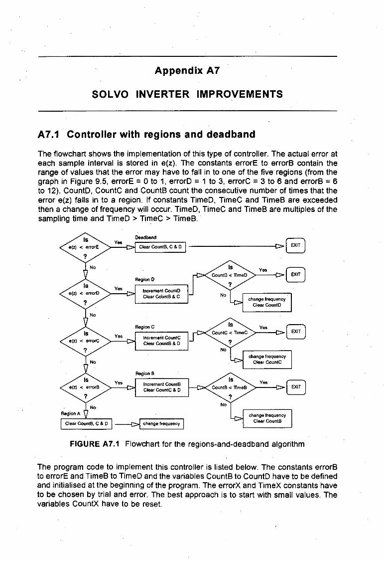
Univers
ity of
Cap
e Tow
n
Appendix A7
SOLVO INVERTER IMPROVEMENTS
A7.1 Controller with regions and deadband
The flowchart shows the implementation of this type of controller. The actual error at each sample interval is stored in e(z). The constants errorE to errors contain the range of values that the error may have to fall in to one of the five regions (from the graph in Figure 9.5, errorE = O to 1, errorD = 1 to 3, errorC = 3 to 6 and errors = 6 to 12). CountD, CountC and Counts count the consecutive number of times that the error e(z) falls in to a region. If constants TimeD, TimeC and Times are exceeded then a change of frequency will occur. TimeD, TimeC and Times are multiples of the sampling time and TimeD > Tin:iec > Times.
Dead band Yes r:;:;:-"')
>--e>t-Cle_ar_eo_un_tB_. c_&_o_ -----------[> LJ
Region 0
Increment CountO Clear COuntB & C
Region C
Yes Increment CountC Clear CountB & 0
Region B
Increment CountB Clear CountC & 0
ClearCountB, C&O ~
Yes r:;:;:-"') >---C>LJ
change frequency Clear CountO
change frequency Clear CountC
Yes r:;:;:-"') >---C>LJ
change frequency Clear CountB
FIGURE A7.1 Flowchart for the regions-and-deadband algorithm
The program code to implement this controller is listed below. The constants errors to errorE and Times to TimeD and the variables Counts to CountD have to be defined and initialised at the beginning of the program. The errorX and Timex constants have to be chosen by trial and error. The best approach is to start with small values. The variables CountX have to be reset.

Univers
ity of
Cap
e Tow
n
308 Appendix A 7: Solvo inverter improvements
. The program code below (italics) must be added to the Timer1 interrupt-routine. It replaces four program code lines.
GREATER: MOV A,SWNEU CLR c SUBB A,SWALT SETB HOCHFL
MOV error,A CJNE A,errorE,AUX_E JMP EXIT
AUX E: JC REG E JMP AUX D
REG E: MOV CountB,#0 MOV CountC,#0 MOV CountD,#0 JMP EXIT
AUX_D: CJNE A,errorD,AUX_DD JMP REG D
AUX DD: JC REG D JMP AUXC
REG D: INC Coun.tD MOV CountB,#0 MOV CountC,#0 MOV A,CountD CJNE 'A, TimeD,POST _ D
POST D: JC EXIT MOV CountD,#0 JMP CHANGE_FREQUENCY
AUX C: MOV A, error CJNE A,errorC,AUX_CC JMP REG C
AUX CC: JC REG C JMP AUX B
REG C: INC CountC MOV CountB,#0 MOV CountD,#0 MOV A,CountC CJNE A, TimeC,POST _ C
POST C: . JC EXIT MOV CountC,#0 JMP CHANGE _FREQUENCY

Univers
ity of
Cap
e Tow
n
Section A7.1: Controller with regions and deadband 309
AUX B: MOV A, error CJNE A,errorB,A UX _BB JMP REG B
AUX BB: JC REG B JMP AUX A
REG B: INC CountB MOV CountC,#0 MOV CountD,#0 . MOV A,CountB CJNE A, TimeB,POST _B
POST B: JC EXIT MOV CountB,#0 JMP CHANGE_FREQUENCY
AUX A: MOV CountB,#0 MOV CountC,#0 MOV CountD,#0 JMP CHANGE_FREQUENCY
Note: The original program uses the address 'HILF' instead of 'EXIT' and 'AKTST' instead of 'CHANGE_FREQUENCY'. The original addresses should be used. The first four lines of program code after the five original lines at the top have to be deleted to fit into the existing program. ·
This controller would handle installations which have a faster settling time (smaller RC) without any problem. If an installation has a longer settling time then the array voltage oscillations would start occuring and the algorithm requires retuning.

Univers
ity of
Cap
e Tow
n
31 0 Appendix A 7: So/vo inverter improvements
A7.2 Incorrect array operating point
Figure A7 .2 shows the same flowchart as in the main text but more specific for the Solvo program.The explanations are therefore the same.
increment Sample
set CutnWait flag
RETURN
FIGIURE A7.2 Flowchart for avoiding incorrect array operating points
The program code for the subroutine is listed below. Lowadc, Window, Sample, Edge, Watchdog and CutnWait have to be defined and initialised.
LOUSY: MOV A, ST ALT CJNE A,STNEU,ROSES JMP ARE
ROSES: JC ARE MOV A,STNEU
ARE: CJNE A,#2,DARK JMP RED
DARK: JC MOTION
RED: MOV A, WANDEL CJNE A,LOWADC,ZAP 1 JMP NOTLOW
ZAPJ: JC ZAP2 JMP NOTLOW
ZAP2: INC WATCHDOG MOV A, WATCHDOG CJNE A,EDGE,CASEJ JMP NOTLOW
CASEJ: JC NOTLOW SETB CUTNWAIT
NOTLOW: INC SAMPLE

Univers
ity of
Cap
e Tow
n
CASE2: MOTION:
END LY:
Section A 7. 3: Minimum power threshold 311
MOV CJNE JMP JC MOV MOV RET
A, SAMPLE A, WINDOW,CASE2 END LY END LY SAMPLE,#0 WATCHDOG,#0
This subroutine is called in the Timer1 interrupt routine after the array voltage has been read in at the ADC. Lowadc should be chosen to be about 50% to 60% of the open-circuit voltage. Window should not be less than 100 and Edge should always be half of the Window value. If the Watchdog counts more occurences of low voltage than the value held in Edge then the CutnWait flag is set. This flag is continuously scanned in the main program. When the flag is true then the inverter output is inhibited and the program enters a waitstate of a set time.
This routine would reduce considerably if the controller was implemented correctly so that the array voltage oscillations would reduce to about ±1 V. Then there would be no need to take an average of the array voltage.
A7.3 Minimum power threshold
The flowchart in Figure A7.3 shows the program flow for the Solvo inverter. First the lowest major gear is detected (Stalt/Stneu) and then whether the program has entered the active gears (major gear 5 to 15; major gear O to 4 do not generate an output but the program still runs through them. As long as the program remains between Actgear and Lowgear (largest unwanted gear) the Ticker variable will be incremented until it reaches a value larger than Prevail.
The program code for the subroutine is listed below. The routine is called from Timer1. Actgear, Lowgear, Ticker, Prevail and CutnWait have to be defined and initialised. Actgear always takes the value of the first active gear. This is presently gear 5. The program changes as suggested in section A7.5 would have Actgear equal to zero. Lowgear should be set to gear 6 or 7 for the present program. The following has to hold true for the constant 'Prevail': Prevail> (Lowgear - Actgear +1) x 16.
TOOSLOW:
SOHO:
GETON:
VERIFY: MOVEON:
MOV CJNE JMP JC MOV CJNE JMP JC CJNE JMP
A,STALT A,STNEU,SOHO GETON GETON A,STNEU A,ACTGEAR, VERIFY MOVEON NAUGHT A,LOWGEAR, TESTFO GROW

Univers
ity of
Cap
e Tow
n
312 A~pendix A 7: Solvo inverter improvements
TESTFO: JC GROW NAUGHT: MOV TICKER,#0
JMP ENDSLOW
GROW: INC TICKER MOV A, TICKER CJNE A,PREVAIL,OUTRO JMP ENDSLOW
OUTRO: JNC SETF JMP ENDSLOW
SETF: SETB CUTNWAIT
ENDSLOW: RET
A <-Stneu
increment Ticker
clear Ticker
Yes
set CutnWait flag
RETURN
FIGUIRE A7.3 Flowchart for the detection of a minimum power threshold
This program code cannot be implemented before the algorithm has not been improved since the array voltage oscillations also result in frequency oscillations (see Figure 9.2).

Univers
ity of
Cap
e Tow
n
Section A7.4: Higher resolution voffage to hertz relation 313
A7 .4 Higher resolution voltage to hertz relation
The increase in resolution for the voltage to hertz relation requires one additional variable. This variable must continuously update it!)elf to hold the value of the minor gear in which the inverter program presently resides (the program has 16 major gears and within each major gear it has 16 minor gears). The variable (Minorgear) can therefore only hold values between zero· and fifteen.
The variable has to follow the· minor gear while the inverter remains in a major gear and has to assume either zero or fifteen when the program changes to another major gear. The flowchart in Figure A7.4 shows how the variable (Minorgear) keeps track of the actual minor gear.
Yes
Clear Minorgear
Yes
No
Yes
Increment Minorgear
Minorgear ~ 15
Decrement Minorgear
FIGURE A7.4 Flowchart for keeping track of the minor gear
'Stneu' (new major gear), 'Stalt' (old major gear), 'Swneu' (array voltage) and 'Swait' (reference voltage) are present variables in the program. The routine in the flowchart is executed every time the program decides how to drive the motor. It has to find whether there is a change between major gears (is Stneu = Stalt ?) and if so if the gears are decreasing or increasing. If there was no change in major gears it has to find out whether the frequency is increasing or decreasing which it can do by comparing the array voltage to the reference voltage.
Since the program does this process as well only a few appropriate codes have to be added. The variable Minorgear has to be defined and initialised (to zero). In the Timer1 interrupt routine the following line (italics) has to be added after the existing code line:
INC INC
DEC DEC
SCHFREQ MINORGEAR
SCHFREQ MINORGEAR

Univers
ity of
Cap
e Tow
n
314 Appendix A 7: So/vo inverter improvements
INC ST ALT MOV MINORGEAR , #0
DEC ST ALT MOV MINORGEAR, 15
The variablle Minorgear is used in a subroutine called from Timer1 which assigns the required values to the IC that generates the PWM signals. The routine is called 'Wertzu'. V\fhere necessary the following flowchart can be implemented to increase the resolution 1of the voltage to hertz relation.
Yes ">--1::>1 Select 90V PWM table
Yes ">---C>I Select 94V PWM table
No
Select 97V PWM table
FIGURE A7.5 Flowchart for the assigning of a higher resolution voltage to hertz relation
In this example the sixteen minor gears are divided into three submajor-gear categories. Each of the three can now be assigned a different voltage. As a further example, say major gear 14 should be devided into three sub-major frequency ranges. The program would have the following .additions (in italics):
ST14:
ST14A
ST14B: ST14BB:
ST14C:
MOV CJNE JNC MOV MOV JMP CJNE JNC MOV MOV JMP MOV MOV
A,MINORGEAR A,#6,ST14A STJ4B LOWTAB,#LOW TAB90 HIGHTAB,#HIGH TAB90 RESTJ4 A,#JJ,ST14BB ST14C LOWTAB,#LOW TAB94 HIGHTAB,#H/GH TAB94 REST14 LOWTAB,#LOW TAB97 HIGHT AB,#HIGH TAB97

Univers
ity of
Cap
e Tow
n
Section A 7. 5: Solvo inverter switching frequency 315
REST14: MOV MOV MOV MOV MOV MOV JMP
STSTNEU,#48 PHINEU,#16 PH2NEU,#32 ZANEU,#4 TMIN,#OB7H TMAX,#OA8H EXIT
TAB90, TAB94 and TAB97 are addresses of voltage look-up tables which contain PWM ratios for different voltage amplitudes.
This program code can be added to any of the sixteen major gears. It was suggested in the main text that major gears 1 O to 12 should be divided into two sub-major gears and major gears 13 to 15 into three sub-major gears. The program code above can be added at the appropriate place in the program.
A7.5 Solvo inverter switching frequency
The table below contains the values for a program that will have a generally lower switching frequency.
TABLE A7.1 Program values for a lower switching frequency
Major Tmax Tmln Tmax Tmln f • ..,,,,n fa-max fmtn fmax m' I N gear [ps] [ps] [hex] [hex] [kHz] [kHz] [Hz] [Hz]
0 60 45 C4 03 16.7 22.2 5.0 6.6 48 70 1 68 53 BC CB 14.7 18.9 6.7 8.7 48 45 2 76 61 B4 C3 13.2 16.4 8.8 11.0 48 31 3 75 60 B5 C4 13.3 16.7 11.1 13.9 48 25 4 99 84 90 AC 10.1 11.9 14.0 16.5 48 15 5 103 88 99 AB 9.7 11.4 16.9 19.7 48 12 6 116 101 BC 9B 8.6 9.9 20.0 22.9 48 9 7 112 97 90 9F 8.9 10.3 23.3 26.8 48 8 8 110 95 92 A1 9.1 10.5 27.1 31.3 48 7 9 110 95 92 A1 9.1 10.5 31.6 36.5 48 6 10 112 97 90 9F 8.9 10.3 37.2 43.0 48 5 11 120 105 88 97 8.3 9.5 43.4 49.6 48 4 12 112 97 90 9F 8.9 10.3 49.6 57.3 36 5 13 121 106 87 96 8.3 9.4 57.4 65.6 36 4 14 127 112 81 90 7.9 8.9 65.6 74.4 30 4 15 124 109 84 93 8.1 9.2 74.7 84.9 36 3
Tis the period of the switching frequency. The hexadecimal values are used as down counters in the program. f s is the switching frequency and f is the inverter output frequency. m'1 is the scaled frequency modulation index and N is number of times that the equal width-pulses are repeated. The actual frequency modulation index is m'1 x N.

Univers
ity of
Cap
e Tow
n
316 Appendix Al: Solvo inverter improvements ·
The fundamental frequency is calculated with the following equation:
1 f = ----m1xNx T
(A7.1)
The assigning of frequency ranges to the major gear is slightly tedious and lacks some flexibility. The aim was to stay below a 1 OkHz switching frequency but that is not possible at lower fundamental frequency else the frequency range becomes so narrow that more major gears would be required (but are not available) to span a frequency range from 5Hz to 85Hz.
The switching frequency therefore increases above 10.5kHz in the frequency range from 20Hz to 5Hz. That is fine since the inverter will operate most of the time above 40Hz. Thi~ switching frequency range for the main operating range is therefore 7.9kHz to 10.5kHz. All sixteen major gears are now used which is not as such essential since the frequency resolution is good. Using more major gears does not improve the voltage to hertz resolution.

Univers
ity of
Cap
e Tow
n
Appendix AS
PV PUMP SIMULATION PROGRAM
The information in this appendix is based on 'PVPUMP - A user's manual' by Davis (1994a) and 'Report on RAPS water pumping project' also by Davis (1994b). For detailed information on the PV pump simulation program, both the manual and the report should be consulted.
AS.1 Overview
The PV pump simulation program can be used to predict the water delivery of photovoltaic water pumps at different sites on an hourly, daily and monthly basis. This program has been written by Mark Davis for the Energy for Development Research Centre at the University of Cape Town. The following is a brief description of the program, the simulation conditions, the equations used by the program for the subsystem performance data and the assumptions and limitations of the program.
The program relies on a database of different types of PV modules and on a database of long-term meteorological weather data which consists of hourly records of the horizontal global irradiance, the horizontal diffuse irradiance, the ambient temperature and the wind speed. The program uses a set of yearly data that has been selected from the long term data to represent typical irradiation patterns. In addition, an extensive database provides the subsystem performance data for various available PV pumps at different heads and for different array configurations. Subsystem data for other PV pumps can be added if the necessary information is available.
A simulation requires the user to specify the site conditions (such as static head, locality etc) as well as the selection of the PV pump system and the PV array configuration.
The program calculates the plane of array irradiance using the enhanced Perez model and the cell temperature using an algorithm developed by Fuentes. The array output is calculated using an analytical model developed by Rauschenbach. These methods are discussed in detail by Davis (1994b). The array operating point is calculated as the intersection of the array supply function and the load curve. The latter is a function of the generic type of system, for example AC with MPPT, DC with linear current booster etc. The calculation produces flowrate results on an hourly basis.
Depending on the program settings the data is presented either hourly (irradiance, short-circuit current, operating current, operating voltage, efficiency and flowrate) or in terms of daily and monthly averages (daily irradiation, daily volume flow from which the monthly and annual averages are processed).
The program offers a supply versus demand analysis of the water-reservoir tank levels
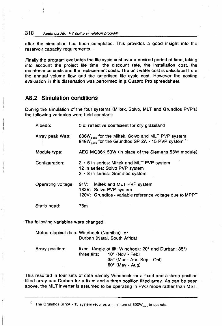
Univers
ity of
Cap
e Tow
n
. j
318 Appendix AB: PV pump simulation program
after the simulation has been completed. This provides a good insight into the reservoir capacity requirements ..
Finally thE! program evaluates the life cycle cost over a desired period of time, taking into acco1unt the project life time, the discount rate, the installation cost, the maintenance costs and the replacement costs. The unit water cost is calculated from the annual volume flow and the amortised life cycle cost. However the costing evaluation in this dissertation was performed in ~ Quattro Pro spreadsheet.
AS .2 Simulation conditions
During the simulation of the four systems (Miltek, Solve, MLT and Grundfos PVP's) the following variables were held constant:
Albedo:
Array peak Watt: I
Module type:
Configuration:
Operating voltage:
Static head:
0.2; reflective coefficient for dry grassland
636Wpaak for the Miltek, Solve and MLT PVP system 848W peak for the Grundfos SP 2A - 15 PVP system 0
AEG MQ36K 53W (in place of the Siemens 53W module)
2 x 6 in series: Miltek and MLT PVP system 12 in series: Solve PVP system 2 x 8 in series: Grundfos system
91V: Miltek and MLT PVP system 182V: Solve PVP system 120V: Grundfos - variable reference voltage due to MPPT
76m
The following variables were changed:
Metieorological data: Windhoek (Namibia) or Durban (Natal, South Africa)
Array position: fixed (Angle of tilt: Windhoek: 20° and Durban: 35°) three tilts: 10° (Nov - Feb)
35° (Mar - Apr, Sep - Oct) 60° (May - Aug)
This resulted in four sets of data namely Windhoek for a fixed and a three position tilted array and Durban for a fixed and a three position tilted array. As can be seen above, the ML T inverter is assumed to be operating in FVO mode rather than MST.
1> The Grundfos SP2A - 15 system requires a minimum of 800Wpeak to operate.

Univers
ity of
Cap
e Tow
n
Section AB.3: Fitted equations used by simulation program 319
AS.3 Fitted equations used by simulation program
The simulation program requires the subsystem efficiency curves of a PV pump over its input power range. These curves are specified as two second order polynomials. The threshold power from one polynomial to the other is usually chosen to be the point of largest discontinuity in the curve.
The table below specifies the subsystem equations for the .four PVP systems that are used in the simulations. The minimum (min) and the maximum (max) subsystem input power values are specified. Two equations for subsystem efficiency (E1 and E2) are listed where equation E1 is valid between min and the threshold Tand equation E2 is valid between T and max.
TABLE AS.1 List of fitted subsystem equations with threshold specifications
PVP Equations and threshold specifications subsystem
Miltek: Min: 81 T: 240
Max: 550 E1: - 39.27 + 0.685xP - 0.00165xP2
E2: - 4.48 + 0.225xP - 0.00027xP2
iJ Load-line: 0.05xl0 + 0.4
Solvo: Min: 140 T: 270
Max: 550 E1: - 147.38 + 1.336xP - 0.00256xP2
E2: - 0.37 + 0.154xP - 0.00017xP2
MLT: Min: 190 T: 250
Max: 550 E1: - 458.42 + 4.196xP - 0.00915xP2
E2: - 52.22 + 0.389xP - 0.00043xP2
Grundfos: 21 Min: 480 T: 850
Max: 1800 E1: - 98.77 + 0.286xP - 0.00016xP2
E2: 17.72 + 0.023xP - 0.0000082xP2
11 The load-line is used by the simulation program to evaluate the array operating point once the Miltek converter enters into direct mode. ·
21 The Grundfos data (amongst others) is provided with the PVP simulation package and has been derived from manufacturers specifications.
[W) [W) [W) [%] [%) [A)
[W) [W) [W) [%) [%]
[W) [W) [W] [%) [%]
[W) [W) [W) [%] [%]

Univers
ity of
Cap
e Tow
n
320 Appendix AB: PV pump simulation program
AB.4 Assumptions contained in the simulation
The error sources and the limitations of the simulation procedure are discussed in detail by Davis (1994b). Error sources are found in the weather data, the array output model anid the pump subsystem performance models. Limitations are mainly experienced in the· consideration of the past weather data as being representative and in the partly random components of some of the system characteristics.
Most of these errors and limitations are not applicable to the category of simulations performed since the simulation results are used mainly for comparative purposes and not for the performance prediction of a single PVP system. Therefore the limitations of the weather data in terms of potentially low sequential irradiation intervals are not of serious concern. Nor are the inaccuracies in the array output model.
The errors that will have the largest impact on the comparison are the errors in the · determination of the subsystem efficiency characteristics. Variations have occurred during tho acquisition of data for the three tested systems especially in terms of the start-up conditions. If incorrectly assessed this might favour or disfavour a particular PVP system in the comparison. Another factor is that the subsystem efficiency characteristics, no matter how accurate, represents one system only and not the charact~ristics of a number of same model PVP systems.
The simullation introduces an error by assuming that the head is constant. In the case of the tested PVP systems a head variation of 2m was measured due to drawdown. The head loss variations due to flowrate changes were measured to be negligible. The error due to drawdown is about 1.3% but as all four systems have been assumed to operate at constant head the error is reduced in the comparison.

Univers
ity of
Cap
e Tow
n
Appendix A9
COSTING EQUATIONS
The method with which the cost has been calculated is presented here. The information has been extracted from Cowan (1992).
Life cycle cost
. The life cycle cost (LCC) includes all the costs incurred over the project lifetime (SL) of the photovoltaic pump, which is usually taken as twenty years. The LCC includes the initial capital cost, the installation cost, the annual maintenance cost and replacement costs. The operation costs are zero since a PV system does not require any fuel.
All the future costs are reduced to their present value by a rate which is equivalent to the opportunity cost of the capital investment (which is the cost of holding capital rather than investing it). This rate is referred to as the real discount rate (dr) which can be taken to be the difference between the interest rate and the inflation rate. The present value (PVal) is calculated as follows:
PVal = C x [ 1 ~ dr r (A9.1)
C is the cost in terms of today's money which is being incurred n years from the present.
The LCC is calculated as follows:
SL SL LCC = cln/tltJi + cmtal + .E M + .E R (A9.2)
n•1 n-1
where Cinitiai and C;nstall are the total initial and installation cost respectively. M·and R
are the annual maintenance and replacement costs respectively. Both have been reduced to their present yearly value with equation A9.1 over a period of one to 20 (SL) years. The replacement cost must incorporate the salvage value of the replaced part or component.
The assumptions for the LCC are that the interest and the inflation rate remain constant, that the rate of escalation (which is the price escalation above the inflation rate) is zero and that the maintenance and replacement costs have been correctly assessed.

Univers
ity of
Cap
e Tow
n
\~/
322 Appendix A9: Costing equations
Unit waJer cost
The unit water cost is useful when a few PVP's are compared in terms of cost. The unit water cost takes the cost of the system and the water delivered into account. The units are in cents/m 3
• In order to evaluate the unit water cost the life cycle cost has to be amortiseg into annual amounts first.
p = LCC x [ (1 + /)SL x '] . (1+/)SL-1
(A9.3)
P is the amortised annual amount, SL is the project lifetime (20 years) and i is the interest rate. The real interest rate is taken to be the same as the real discount rate used in equation A9.1.
The unit water cost [cents/m3 ] is calculated by:
unit wst8r cost = __ P __ Q vri: tlllflutll
where Qvol: annual is the total amount of water pumped per year [m 3 ].
(A9.4)
In cases where the PVP's that are being compared are not delivering the water at the same static head the unit water cost can be stated as cents/m4 where the unit water cost as calculated in equation A9.4 is divided by the static head.