BioMedSigProcAna

Event Detection:

Qrs-Complexes in Ecg Signals

Josef GoetteBern University of Applied Sciences, Biel/Bienne

Institute of Human Centered Engineering - microLabJosef.Goette@bfh.ch

February 13, 2018

Contents

1 Introduction 1

2 Qrs Detection 32.1 General Structure of Qrs Detector . . . . . . . . 32.2 Simplest: Derivative-Based Ideas . . . . . . . . . 102.3 Aside: “Integer” Filters . . . . . . . . . . . . . . 142.4 The Pan-Tompkins Algorithm . . . . . . . . . . . 29

References 57

6 EventDet i 2018

BioMedSigProcAna

c©Josef Goette, 2007–2018

All rights reserved. This work may not be translated or copied in

whole or in part without the written permission by the author, except

for brief excerpts in connection with reviews or scholarly analysis.

Use in connection with any form of information storage and retrieval,

electronic adaptation, computer software is forbidden.

6 EventDet ii 2018

BioMedSigProcAna

1 Introduction

Events and Epochs

• biomedical signals carry signatures of physiological events

• epoch = part of a biomedical signal related to a specificevent

• biomedical signal analysis

– for monitoring and diagnosis

– requires identification of epochs

– requires investigation of related events

• once an event has been identified, the corresponding wave-form may be segmented & analyzed in terms of

– amplitude

– wave shape (morphology)

– time duration

– time intervals between events

– energy distribution

– frequency content

– . . . and many more

• therefore: event detection is an important step in biomed-ical signal analysis

6 EventDet 1 2018

BioMedSigProcAna

Examples of Events: Waves in Ecg’s

0.2 0.4 0.6 0.8 1 1.2 1.4 1.6 1.8 2−2

−1

0

1

2

P

Q

R

S

T

P

time in seconds

EC

G

noisy ECG signal (random noise)

P wave: Duration less than 120 msec with frequencies below10–15 Hz.

Pq segment: Lasts about 80 msec; is a “non-event”

Qrs wave: Lasts about 70–110 msec, frequencies mostly con-centrated in the interval 10–50 Hz

T wave: Has frequency content similar to that of the P wave.

St segment: Duration is usually about 100–120 msec and isnormally flat; is a “non-event”

For the various waves in the Ecg signal we have a summaryof the main attributes in [Goe18c, Section 2]. You find a more in-depth treatment in [SL05, Section 6.2.3] and in [Ran02], whereyou find, besides more general information, in Section 4.2.1 adiscussion targeted to event detection.

6 EventDet 2 2018

BioMedSigProcAna

2 Qrs Detection

2.1 General Structure of Qrs Detector

General Requirements on a Qrs Detector

• must be able to detect a large number of different Qrsmorphologies to be clinical useful

• must be able to follow

– sudden changes

– gradual changes

in prevailing Qrs morphology

• must not lock onto certain types of rhythm, but treat nextpossible event as if anything could happen next

6 EventDet 3 2018

BioMedSigProcAna

Detector-Critical Types of Noise and Artifacts

• noise might be in nature

– highly transient

– or persistent (e.g. power-line interference)

• problem of conditioning Ecg signals w.r.t. noise has beentreated

• however, term “noise” has a somewhat different meaningwhen considered form the Qrs-detection viewpoint

– P- and T-wave must here be treated as noise

– noise might have physiological as well as technicalorigins

We refer to our accompanying document [Goe18a] for theproblem of conditioning Ecg signals with respect to noise.

6 EventDet 4 2018

BioMedSigProcAna

Classification of Noise Problems

signal and noise problems in Qrs detection can be classified intotwo main categories with further sub-classification

• changes in morphology (including amplitude changes)

– of physiological origin

– due to technical problems

• occurrence of noise

– Ecg signals with large P- and T-waves

– noise of myoelectric origin

– noise due to transient artifacts (mainly due to elec-trode problems)

If in an Ecg, the P-waves and/or the T-waves are enlargeddue to distortions, they might be miss-interpreted as Qrs com-plexes.

Muscles produce noise, called above noise of myoelectric ori-gin. Recalling that the heart is just a very special muscle, weunderstand that myoelectric noise will disturb, among others,Ecg measurements.

6 EventDet 5 2018

BioMedSigProcAna

General Block-Diagram of Qrs Detectors

• most Qrs detectors described in the literature: developedfrom ad hoc reasoning and experimental insight

• general detector forms

– pre-processor: enhance Qrs complex while suppress-ing noise and artifacts

– usually: linear filtering followed by a non-linear trans-formation

– decision rule for detection

x[n] linearfiltering

nonlineartransformation

decisionrule

θi

prepocessor

• x[n] = Ecg-signal input to detector

• θi, i = 1, 2, . . . = series of occurrence-times of detectedQrs complexes

The goal of the linear filter in the above block diagram isto reduce artifacts while keeping the essential spectral contentsof the Qrs complex. It has a bandpass characteristics and re-duces the influence of muscle noise, P- and T-waves, power-lineinterferences and baseline wander. The center frequency of thefilter varies from 15 Hz to 25 Hz with a bandwidth varying from

6 EventDet 6 2018

BioMedSigProcAna

5 Hz to 10 Hz. Note that waveform distortion is, in contrast toother types of Ecg-signal filtering, not a critical issue in Qrsdetection; instead, the goal is to improve signal-to-noise ratio toachieve good detector performance.

The goal of the nonlinear transformation is to further en-hance the Qrs complex relative to the remaining backgroundnoise. Additionally, it must transform each Qrs complex into asingle positive peak that is better suited to threshold detection.In general, the nonlinear transformation might be memory-less(static)—rectification or squaring are examples—or a more com-plex transformation involving memory. Note, however, that notall Qrs detectors use a nonlinear transformation in their pre-processing stage.

The goal of the block named decision rule is to perform,based on the output of the pre-processor, a test on whether ata certain time a Qrs complex is present or not. The decisionrule might be implemented as simple as an amplitude thresh-old procedure, but it may perform additional tests, for exampleon reasonable durations of certain waveforms, to obtain betterimmunity against various types of noise.

Qrs detectors are usually designed to detect heartbeats.They rarely need to produce occurrence times of the Qrs com-plexes with high resolution in time. If time resolution is nev-ertheless important, it may be necessary to improve the initialresolution with algorithms that perform time alignment of thedetected beats and thus reduce the problem of smearing whichmight occur when computing the ensemble average of severalbeats (recall the synchronized averaging, which we have dis-cussed in [Goe18a]).

6 EventDet 7 2018

BioMedSigProcAna

Qrs Detection as an Estimation Problem

• theoretical justification of Qrs-detector structure on page 6

– investigate statistical models of Ecg signals

– use maximum-likelihood estimation techniques to de-rive detector structures corresponding to the signalmodel of interest

• example model: unknown occurrence-time and amplitude

x[n] =

v[n] , 0 ≤ n ≤ θ − 1 ,

as[n − θ] + v[n] , θ ≤ n ≤ θ + D − 1 ,

v[n] , θ + D ≤ n ≤ N − 1 ,

where N = length of observation intervalv[n] = noises[n] = Qrs-complex, known morphology, duration

θ = unknown occurrence time of Qrs-complexa = unknown amplitude of Qrs-complex

Sornmo and Laguna [SL05] discuss in Section 7.4 Qrs detec-tion in a more theoretically oriented manner. With the proposedsignal model shown above, it is then feasible to estimate the un-

known occurrence time θ and the unknown amplitude a of theQrs-complex. The notion “Qrs detection” suggests, however,that we are faced with a detection problem instead of an esti-

mation problem. It is indeed true that the problem consideredin [SL05] can likewise be formulated as a detection problem;

6 EventDet 8 2018

BioMedSigProcAna

Sornmo and Laguna discuss these different viewpoints and statethat both of them essentially lead to same detector structures,for details see [SL05, p. 488].

Qrs Detection as an Estimation Problem (2)

• for considered model, theory shows that the Qrs detectormust use as nonlinear transformation a squaring operation

• if example model has more a priori knowledge

– unknown amplitude is constrained to known interval:

– 0 < a1 < a < a2 , with known a1 and a1

then theory shows that the Qrs detector must use as non-linear transformation a rectifier

By generalizing the above Ecg-signal model to a model withunknown occurrence-time, unknown amplitude, and unknown

duration of the Qrs complex, Sornmo and Laguna [SL05] derivethe optimum Qrs-complex detector structure.

6 EventDet 9 2018

BioMedSigProcAna

2.2 Simplest: Derivative-Based Ideas

Using First- and Second Derivatives

• differentiation forms basis of many Qrs detection algo-rithms

• differentiation = basically a highpass filter

– amplifies higher frequencies that are characteristic forthe Qrs complex

– attenuates lower frequencies that are characteristicfor P- and T-waves

– attenuates low frequencies of baseline wander

• however: differentiation also amplifies higher frequenciesdue to noise ; additional significant smoothing is required

• an algorithm based on first and second derivatives, withsmoothing included

– by Balda et. al. in 1977

– modified by Ahlstom and Tompkins for high-speedapplications in 1983

– additionally modified by Friesen et. al. 1990

The references cited in the above slide are [BDD+77], [AT83],and [FJJ+90].

6 EventDet 10 2018

BioMedSigProcAna

The Algorithm: Pre-Processing

• let x[n] = input to and y[n] = output from pre-processingstage of algorithm

• use for pre-processing a linear combination of first- andsecond derivative

• first derivative: approximated as absolute value of three-point first difference

y0[n] =∣∣∣x[n] − x[n − 2]

∣∣∣ .

• second derivative: approximated as absolute value of three-point first difference of three-point first differences

y1[n] =∣∣∣x[n] − 2x[n − 2] + x[n − 4]

∣∣∣ .

• output y[n] of pre-processing stage as linear combination

y[n] = 1.3 · y0[n] + 1.1 · y1[n]

To understand the rationals behind the given approximationof the first derivative, we start with a first-difference operator:

δ1[n] = x[n] − x[n − 1] •—• ∆1(z) =(1 − z−1

)X(z) .

6 EventDet 11 2018

BioMedSigProcAna

This filter has a zero at z = 1—at Dc frequency—and has amagnitude response of 2 sin (ω/2). For sufficiently low frequen-cies ω, it approximates the derivative operation as we see from2 sin (ω/2) ≈ 2ω/2 = ω. To obtain a smoothing such that high-frequency noise is not too much amplified, we post-process thesequence δ1[n] by a two-point moving-average filter having trans-fer function (1 + z−1):1

y0[n] = δ1[n] + δ1[n − 1]

=(x[n] − x[n − 1]

)+(x[n − 1] − x[n − 2]

)

=(x[n] − x[n − 2]

).

In the z-transformation domain we equivalently have

Y0(z) =(1 + z−1

)∆1(z)

=(1 + z−1

)(1 − z−1

)X(z)

=(1 − z−2

)X(z) .

Clearly, the complete filter (1 − z−2) has one zero at z = 1—atfrequency ω = 0—, which approximates the derivative, and asecond zero at z = −1—at frequency ω = ±π—, which sup-presses high frequency noise. The magnitude response of the fil-ter is 2 sin (ω); for low frequencies we again have 2 sin (ω) ≈ 2ω,which approximates a derivative with a gain 2.

For the approximation of the second derivative consider thesequence y0[n] being the output of a three-point first differencefilter: y0[n] = x[n] − x[n − 2]. Processing this sequence by

1We denote the output of this processing step by y0[n] to distinguish itfrom y0[n], which we use in the slide on page 11, and which is the absolutevalue of y0[n].

6 EventDet 12 2018

BioMedSigProcAna

another three-point first difference filter, we obtain2

y1[n] = y0[n] − y0[n − 2]

=(x[n] − x[n − 2]

)−(x[n − 2] − x[n − 4]

)

=(x[n] − 2x[n − 2] + x[n − 4

).

The Algorithm: Decision Rule

• threshold y[n] = output of pre-processing with a threshold-value of 1.0

• if y[n0] ≥ 1.0 for a certain n0, then compare next 8 samplesto threshold

• if 6 or more of these 8 samples pass threshold test, thentake the 8-samples segment as part of a Qrs complex

• advantage: additionally to detecting Qrs complexes, thealgorithm produces a pulse that is proportional in widthto the Qrs complex

• disadvantage: the method is extremely sensitive to high-frequency noise

2Again, we denote the output of this processing step by y1[n] to distin-guish it from y1[n], which we use in the slide on page 11, and which is theabsolute value of y1[n].

6 EventDet 13 2018

BioMedSigProcAna

2.3 Aside: “Integer” Filters

Motivation

• in real-time operations of digital filters

– many filter designs are unsatisfactory

– because huge computation-time requirements

– surely if implemented in floating-point operations

– but often also if implemented in fixed-point opera-tions

• integer filters are a special class of filters having only in-teger coefficients

• here more special: coefficients ∈ {0,±1,±2}

• here even more special: a preparation to the Pan-Tompkinsalgorithm

We admit that we are not sure about the generality of thenotion “integer filters.” We feel that the notion “integer filters”used in the signal processing community is more general thanthe same notion often used in the literature on biomedical signalprocessing. Our present discussion treats filters in the morerestricted meaning as given, for example, in [Tom93]—see thereChapter 7 entitled “Integer Filters,” but also see its Chapter 12on Qrs detection.

For Qrs detection, for example, it is crucial that the Qrscomplex as well as P- and T-waves remain unchanged. This

6 EventDet 14 2018

BioMedSigProcAna

demand on preservation of signal forms calls for linear-phasefilters, which must be Fir filters. “Integer” filters as we discussthem here are Fir filters with recursive implementations.

The slide on the previous page 14 states that our “integer”filters have only coefficients being 0, ±1, and ±2. This is notthe full truth: The basic blocks that we consider have suchcoefficients, but cascading these basic blocks leads to additionalcoefficient values, see page 28.

Here an “aside to the aside” is in order: There is anotherspecial family of filters with coefficients that do not need multi-plications when they execute. These Fir filters are called bino-

mial filters, and the family is based on the very simple lowpassor highpass filters H1(z) = (1 + z−1), or H1(z) = (1 − z−1),respectively. If such a H1(·) is cascaded once, we obtain—forthe lowpass situation—H2(z) = H1(z) ·H1(z) = 1+2z−1 + z−2;if we cascade one more basic block H1(·), we obtain H3(z) =H3

1 (z) = 1 + 3z−1 + 3z−2 + z−3; and so on—see Pascal’s trian-gle. Likewise we might also use the highpass basic block in thecascade, or we might even mix lowpass basic blocks (1 + z−1)with highpass basic blocks (1 − z−1) in the cascade.3 In anycase we should note that the cascaded-blocks filter has neverto multiply signal samples with coefficients when executing, butthe overall filter will realize binomial coefficient values—againrecall Pascal’s triangle.

3What filter type results, if we mix lowpass and highpass basic blocks?You might want to experiment with Matlab.

6 EventDet 15 2018

BioMedSigProcAna

Simple Example

• transfer function

H(z) =1 − z−6

1 − z−1 + z−2=

z6 − 1

z4 (z2 − z + 1)=

N(z)

D(z)

• zeros

N(zz) = z6z − 1 ≡ 0

; zz = ej·k·2π/6 , k = 0, 1, . . . , 5 = 6-th roots of unity

1

j

.....

.....

.....

.....

.....

.....

................................................................

.................

.........................

...............................................................................................................................................................................................................................................................................................................................................................................................................

........................................................................................................................................c

cc

c

cc

zeros: 6-th roots of unity

Note that the transfer function of the above example definesa filter that has only coefficients ±1.

6 EventDet 16 2018

BioMedSigProcAna

Simple Example (cont’d)

• poles zp1 = ρejϕ, zp2 = ρe−jϕ = z∗p1, zpk = 0, k = 3, . . . , 6

• non-trivial poles

D(zp) = z2p − zp + 1 ≡ 0

(zp − ρejϕ

) (zp − ρe−jϕ

)≡ 0

z2p − ρ︸︷︷︸

≡ 1

(ejϕ + e−jϕ

)︸ ︷︷ ︸= 2 cosϕ ≡ 1︸ ︷︷ ︸; ϕ = 60◦

zp + ρ2

︸ ︷︷ ︸≡ 1

≡ 0

1

j

.....

.....

.....

.....

.....

.....

................................................................

.................

.........................

...............................................................................................................................................................................................................................................................................................................................................................................................................

........................................................................................................................................

×

×

ejϕ

....................................................................................................................................................................................................................................................................................................

..........60◦

poles zp1,2 = e±jϕ, ϕ = 60◦

6 EventDet 17 2018

BioMedSigProcAna

Simple Example (cont’d)

• pole-zero map of complete filter (poles “eat” zeros)

1

j

.....

.....

.....

.....

.....

.....

................................................................

.................

.........................

...............................................................................................................................................................................................................................................................................................................................................................................................................

........................................................................................................................................c

c

c

c

×4-fold

complete pole-zero map

• transfer function (filter is Fir, linear phase)

H(z) =1 − z−6

1 − z−1 + z−2= 1 + z−1 − z−3 − z−4

To see how we obtain the second form—the non-recursiveform—of the above Fir-filter transfer function, just multiplythe terms that correspond to the remaining zeros and poles:

(1 − z−1

) (1 + z−1

) (1 − ej2π/3z−1

)(1 − e−j2π/3z−1

).

The first pair of terms gives(1 − z−2

), the second pair of terms

gives—we use the formula of Euler together with the resultcos (120◦) = −1/2—the polynomial

(1 + z−1 + z−2

), and we

finally obtain

(1 − z−2

) (1 + z−1 + z−2

)= 1 + z−1 − z−3 − z−4 .

6 EventDet 18 2018

BioMedSigProcAna

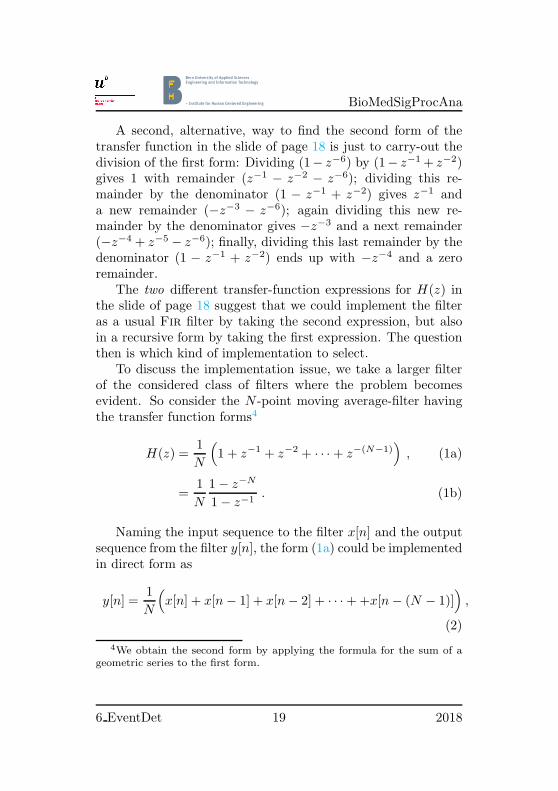
A second, alternative, way to find the second form of thetransfer function in the slide of page 18 is just to carry-out thedivision of the first form: Dividing (1− z−6) by (1− z−1 + z−2)gives 1 with remainder (z−1 − z−2 − z−6); dividing this re-mainder by the denominator (1 − z−1 + z−2) gives z−1 anda new remainder (−z−3 − z−6); again dividing this new re-mainder by the denominator gives −z−3 and a next remainder(−z−4 + z−5 − z−6); finally, dividing this last remainder by thedenominator (1 − z−1 + z−2) ends up with −z−4 and a zeroremainder.

The two different transfer-function expressions for H(z) inthe slide of page 18 suggest that we could implement the filteras a usual Fir filter by taking the second expression, but alsoin a recursive form by taking the first expression. The questionthen is which kind of implementation to select.

To discuss the implementation issue, we take a larger filterof the considered class of filters where the problem becomesevident. So consider the N -point moving average-filter havingthe transfer function forms4

H(z) =1

N

(1 + z−1 + z−2 + · · · + z−(N−1)

), (1a)

=1

N

1 − z−N

1 − z−1. (1b)

Naming the input sequence to the filter x[n] and the outputsequence from the filter y[n], the form (1a) could be implementedin direct form as

y[n] =1

N

(x[n] + x[n − 1] + x[n − 2] + · · · + +x[n − (N − 1)]

),

(2)

4We obtain the second form by applying the formula for the sum of ageometric series to the first form.

6 EventDet 19 2018

BioMedSigProcAna

whereas the form (1b) could be implemented in direct form as

y[n] = y[n − 1] +1

N

(x[n] − x[n − N ]

), (3)

or, in what is called the canonical form, as

w[n] = w[n − 1] + x[n]

y[n] =1

N

(w[n] − w[n − N ]

);

(4)

here in (4) w[n] is a newly introduced interval variable—an in-ternal signal—of the filter.

Comparing the feed-forward implementation (2) to the re-cursive implementations either (3) or (4), we see that the num-ber of operations needed to compute one output sample favorsthe recursive implementations. This lower computational effortis the reason that many books on biomedical signal processingsuggest the recursive implementations.

We note, however, that the recursive implementations mightbecome problems with error accumulation and instability—theimplementations (3) and (4) both have a pole at z = 1, whichis not strictly inside of the unit circle. To get a feeling of whatmight happen, consider the canonical implementation (4) andassume that the input signal is a white-noise signal.5 The equa-tion w[n] = w[n − 1] + x[n] is an accumulator, and accumu-lating a white-noise sequence gives a non-stationary stochasticprocess with a linearly increasing variance, meaning that w[n]must sooner or later become unstable, which is, of course, notacceptable. Similar considerations for the implementation (3)lead to the same conclusions. We do not go into more details,but, instead, refer to [Orf96], where these issues are discussedon pages 402 ff., and which has an Appendix A, pages 728 ff.,discussing discrete-time random signals and their filtering.

5A discrete-time white noise signal is a sequence where any two samplesare uncorrelated.

6 EventDet 20 2018

BioMedSigProcAna

However, an additional note is in order: The transfer func-tion form (1b) shows perfect pole/zero canceling and an imple-mentation based on this form relies on the achievement of thisperfect canceling by the arithmetic used in the implementation.Exact integer arithmetic can achieve it: Both, two’s comple-ment number systems and, more general, any of the residuenumber systems6 have the ability to support error-free arith-metic; in the case of the two’s complement number system, thearithmetic must be performed modulo 2b, that is, with naturaloverflow as we explain in [Goe18b], and in the case of residuenumber systems, the arithmetic is performed in modulo M .

6The two’s complement number system is a member of the family ofresidue number systems, if overflow is correctly treated; see the main text.

6 EventDet 21 2018

BioMedSigProcAna

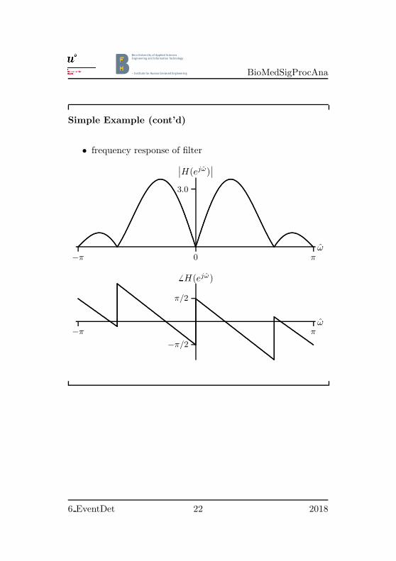
Simple Example (cont’d)

• frequency response of filter

−π 0 π

3.0

.......................................................................................................................................................

...........................................................................................................................................................................................................................................................................................................................................................................................................................................

................................................................................................................................................................................................................................................................................................................................................................................................................................................

.................................................................................................................. ω

∣∣H(ejω)∣∣

−π π

−π/2

π/2...........................................................................................................................................................................................................................................................................................................................................................................................................................................................................................................................................

...............

...............

...............

...............

...............

...............

...............

...............................................................................................................................................................................................................................................................................................................................................................................................................................................................................................................................

ω

6 H(ejω)

6 EventDet 22 2018

BioMedSigProcAna

General: Poles

• complex-conjugate pole-pair on unit circle

zp1 = ejϕ , zp2 = e−jϕ = z∗p1

• thendenominator =

(z − ejϕ

) (z − e−jϕ

)

= z2 −(ejϕ + e−jϕ

)z + 1

= z2 − 2 cosϕz + 1

• has (integer) coefficients ∈ {0,±1,±2} only for

ϕ cosϕ 2 cosϕ

±0◦ 1 2

±60◦ 1/2 1

±90◦ 0 0

±120◦ −1/2 −1

±180◦ −1 −2

Note that the constraints on possible pole locations, whichare given in the above slide, lead to corresponding constraintson the choice of sampling rates if we need to process continuous-time (analog) signals by discrete-time filters,7 and if, therefore,

7Although there are other occasions, we have in biomedical signal pro-cessing always, to our knowledge, the situation where the signals to beprocessed are in the first instance analog signals.

6 EventDet 23 2018

BioMedSigProcAna

natural (physical) frequencies dictate the useful pole locations;see our exemplifying discussion on the the bandpass filter of thePan-Tompkins Qrs detection algorithm given on page 43.

Also note that we compile, later on page 28 and after a cor-responding discussion on “general zeros,” the transfer functionsthat can be realized with “integer filters.”

General: Poles (cont’d)

• zeros of denominator polynomial with integer coefficientsgiven above

• ; possible pole locations

1

j

.....

.....

.....

.....

.....

.....

......................................................................

...................

.................................

.............................................................................................................................................................................................................................................................................................................................................................................................................

..........................................................................................................................×

××

×

××

×

×

2-fold 2-fold

6 EventDet 24 2018

BioMedSigProcAna

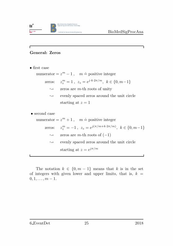
General: Zeros

• first case

numerator = zm − 1 , m = positive integer

zeros: zmz = 1 , zz = ej·k·2π/m, k ∈ {0, m−1}

; zeros are m-th roots of unity

; evenly spaced zeros around the unit circle

starting at z = 1

• second case

numerator = zm + 1 , m = positive integer

zeros: zmz = −1 , zz = ej(π/m+k·2π/m), k ∈ {0, m−1}

; zeros are m-th roots of (−1)

; evenly spaced zeros around the unit circle

starting at z = ejπ/m

The notation k ∈ {0, m − 1} means that k is in the setof integers with given lower and upper limits, that is, k =0, 1, . . . , m − 1.

6 EventDet 25 2018

BioMedSigProcAna

Example: Zeros for zm − 1 = z12 − 1

• for a numerator of type zm − 1

• ; zeros start at z = 1

1

j

.....

.....

.....

.....

.....

.....

......................................................................

...................

.................................

.............................................................................................................................................................................................................................................................................................................................................................................................................

..........................................................................................................................c

c

c

c

c

c

c

c

c

c

c

c

6 EventDet 26 2018

BioMedSigProcAna

Example: Zeros for zm + 1 = z12 + 1

• for a numerator of type zm + 1

• ; zeros start at z = ejπ/m

1

j

.....

.....

.....

.....

.....

.....

......................................................................

...................

.................................

.............................................................................................................................................................................................................................................................................................................................................................................................................

..........................................................................................................................

c

c

c

c

c

c

c

c

c

c

c

c

Note that when the power m is an odd number, the numer-ator zm + 1 always places a zero at ±180◦—at ±π—and thecomplete zero pattern appears “left-right flipped” from the zeropattern of the corresponding numerator zm−1. Take the exam-ple m = 3: In the left-hand side of the graphic below we showthe zeros of z3 − 1, and in its right-hand side we show the zerosof z3 + 1.

1

j

.....

.....

.....

.....

.....

.....

................................................................

.................

.........................

...............................................................................................................................................................................................................................................................................................................................................................................................................

........................................................................................................................................

c

c

c

numerator = z3− 1

1

j

.....

.....

.....

.....

.....

.....

................................................................

.................

.........................

...............................................................................................................................................................................................................................................................................................................................................................................................................

........................................................................................................................................c

c

c

numerator = z3 + 1

6 EventDet 27 2018

BioMedSigProcAna

General: Transfer Functions

• two types of general transfer functions

H1(z) =(1 − z−m)

p

(1 − 2 cosϕz−1 + z−2)q

H2(z) =(1 + z−m)

p

(1 − 2 cosϕz−1 + z−2)q

• where m, p, q = integers

• and where ϕ ∈ {0◦,±60◦,±90◦,±120◦, 180◦}

• note:

raising p & q by equal integer-amounts corresponds to cas-cading of identical filters

As an example for cascading, we start with p = q = 1 andobtain from the above H1(z)

H11(z) =1 − z−m

1 − 2 cosϕz−1 + z−2.

Taking next p = q = 2, we obtain

H12(z) =(1 − z−m)

2

(1 − 2 cosϕz−1 + z−2)2 = H11(z) · H11(z) ,

which is just the cascade of two identical filters with transferfunction H11(z).

6 EventDet 28 2018

BioMedSigProcAna

2.4 The Pan-Tompkins Algorithm

Block Diagram of Pan-Tompkins Algorithm

bandpass

filter

derivative

operator

squaring

operator

mov-win

integrator

• algorithm for Qrs detection in real-time

• referring to general structure on page 6

– linear filtering:

bandpass filter & derivative operator

– nonlinear transformation:

squaring operator & moving-window (mov-win) inte-grator

– decision rule: not shown

• algorithm is intended for Ecg signals that are sampled at200 samples/sec

The algorithm for Qrs detection in real time has been devel-oped by Pan and Tompkins [PT85]; it has further been analyzedand described by Hamilton and Tompkins [HT86]. The algo-rithm recognizes Qrs complexes by analyzing slope and ampli-tude of Ecg signals taking into account the width of appearingEcg waves.

6 EventDet 29 2018

BioMedSigProcAna

We present the algorithm as it is described in [Tom93, Sec-tion 12.5]; you might also want to consult [Ran02, Section 4.3.2]and/or study the original literature [PT85] and [HT86]. Thedescribed form of the algorithm is targeted to an implemen-tation on a microprocessor using integer programming. In thelaboratory exercises we explore variants that might be useful forhardware implementations.

The slide on the previous page 29 states that the describedPan-Tompkins algorithm is intended for discrete-time Ecg sig-nals that have been obtained by sampling the true, continuous-time Ecg signal at a rate of 200 samples/sec. This is true be-cause the algorithm uses “integer” filters that realize pole- andzero locations that are useful for the intended sampling rate,but become unreasonable for different sampling rates; see ourdiscussion starting on page 43.

Because this subsection is quit long, we give an overviewon where you find what. The pre-processing according to theblock diagram shown on page 29 is discussed on pages 31–50;we indicate on page 51 how Pan and Tompkins implement thedecision rule.

For the pre-processing stage we treat the first preprocessingblock, the bandpass filter, on pages 31 to 43. Next we discussthe derivative operator on pages 45 to 46. The squaring operator

follows on page 47, and the final moving-window integrator isdescribed on pages 48 to 50.

6 EventDet 30 2018

BioMedSigProcAna

Bandpass Filter

• isolates the predominant Qrs energy, which is centered inthe 5–15 Hz range

• attenuates the low -frequency characteristics

– of the P- and T-waves

– of baseline wander

• attenuates the high frequencies associated with

– electromyographic noise

– power-line interferences

– measurement noise

• implementation as

– “integer” filter in which poles cancel zeros on unitcircle

– cascade of lowpass and highpass filter

−π 0 π

.................................................................................................................................................................... ω

Lp

−π 0 π

...............................................................................................................................................................................................................................................

...............................................................................................................................................................................................................................................

ω

Hp

−π 0 π

....................................................................................................................

.............................................................................. ω

Bp

6 EventDet 31 2018

BioMedSigProcAna

Bandpass Filter: The Lowpass Part

• consider the transfer function

HLp1(z) =1 − z−6

1 − z−1= 1 + z−1 + z−2 + · · · + z−5

• the Dc gain is (ω = 0 =⇒ z = ej·0 = 1)

HLp1(z = 1) = 1 + z−1 + z−2 + · · · + z−5∣∣z=1

= 6

• the pole-zero map and the magnitude response are

1

j

.....

.....

.....

.....

.....

.....

......................................................................

...................

.................................

.............................................................................................................................................................................................................................................................................................................................................................................................................

..........................................................................................................................c

cc

c

cc

× ×5-fold

−π 0 π

6.0

..............................................................................................................

..........................................................................................................

..............................................................................................................................................................................................................................................................................................................................................................................

...............................................................................................................

........................................................................ ω

∣∣H(ejω)∣∣

We call HLp1(z) a running sum filter to distinguish it froma moving average filter, because it does not take the average; inthe case of HLp1(z) it does not divide by 6.

6 EventDet 32 2018

BioMedSigProcAna

Bandpass Filter: The Lowpass Part (cont’d)

• the complete Lp filter is the scaled cascade of two HLp1(z)

• the cascade HLp1(z) · HLp1(z) =(HLp1(z)

)2has Dc-gain

6 · 6 = 36

• for unity Dc-gain it needs a scaling factor 1/36

• the used scaling factor is 1/32:

– approximates 1/36 to avoid saturation

– can be implemented by a right shift of 5 bit-positions

• the transfer function of the used lowpass filter then is

HLp(z) =1

32

(1 − z−6

1 − z−1

)2

=1

32

1 − 2z−6 + z−12

1 − 2z−1 + z−2=

Y (z)

X(z)

6 EventDet 33 2018

BioMedSigProcAna

Bandpass Filter: The Lowpass Part (cont’d)

• the magnitude response is

−π 0 π

1.0

................................................................................................................................................................................................................................................................................................................................................................................................................................................................................................................................................................................................................................................................................................................................................................................................................................................................... ω

∣∣H(ejω)∣∣

• the difference equation for a recursive implementation is

y[n] = 2y[n−1]− y[n−2] +1

32

(x[n] − 2x[n−6] + x[n−12]

)

Do you see how the difference equation in the above slideresults from the transfer function HLp(z) on the previous page?Do you understand to which form of the given transfer func-tion it corresponds to? How would you write the time-domaindescription for the other form of that transfer function?8

8Hint: For the “other form” you must introduce an “internal signal;”correspondingly, you obtain two (coupled) difference equations.

6 EventDet 34 2018

BioMedSigProcAna

Bandpass Filter: The Highpass Part

• implemented by a delay-complementary transfer function

highpass = delay allpass− lowpass

x[n] delayallpass

+−

y[n]

32-pointmoving average

y1[n]

• delay of M -point moving averager is (M − 1)/2

• for M = 32: half-sample delay 31/2 ; 16 is used

You might want to read more about complementary transferfunctions; [Mit98, pp. 245–249] discusses not only delay-com-plementary transfer functions, but also more general allpass-complementary filters, power-complementary filters and magni-tude-complementary filters. Alternatively, you might use thenewer edition of that book; [Mit06, pp. 391–396] additionallydiscusses doubly-complementary transfer functions, which are atthe same time allpass-complementary and power-complementary.

Concerning the delay of a moving-average Fir filter we havethe following: First consider a pure delay system

y[n] = x[n − n0] ,

6 EventDet 35 2018

BioMedSigProcAna

which delays each sample of the input sequences by n0 samples.The transfer function of this system is H(z) = z−n0 , and itsfrequency response becomes H(ω) = e−jωn0 .

Next consider an M -point moving-average filter. Its transferfunction is

H(z) =1

M

(1 + z−1 + . . . + z−(M−1)

)=

1

M

1 − z−M

1 − z−1.

Its frequency response can be expressed as

H(ω) = H(z = ejω) =1

M

1 − e−jωM

1 − e−jω

=1

M

e−jωM/2(ejωM/2 − e−jωM/2

)

e−jω/2(ejω/2 − e−jω/2

)

=

(1

M

sin(ωM/2)

sin(ω/2)

)

︸ ︷︷ ︸Dirichlet function

e−jω(M−1)/2 ,

where we have used Euler’s formula, and where the indicatedDirichlet function is purely real. We see then that H(ω) is theproduct of two functions, the Dirichlet function and e−jω(M−1)/2,with the latter indicating a shift of (M − 1)/2 samples. Clearly,if the filter length M is an odd integer, (M − 1)/2 becomes aninteger, and the meaning of delaying by an integer number ofsamples is clear. In M is, however, an even integer, (M − 1)/2is not an integer, and the delay needs a special interpretation;[MSY98, pp. 192–194] gives such an interpretation by applyinga discrete-time moving average filter to process continuous-timesignals. To summarize, a half-sample delay has to be interpretedas follows: Think of interpolating the samples of the discrete-time signal by an interpolating continuous-time signal, and thenre-sample that continuous-time signal at half-sample positions.

6 EventDet 36 2018

BioMedSigProcAna

The usage of an allpass with a delay of 16 to approximatethe needed delay of 31/2 leads to a resulting overall highpassfilter that has not exactly a linear phase; see our discussion onpage 38 and the following pages.

Bandpass Filter: The Highpass Part (cont’d)

• the 32-point moving average filter has transfer function

HMA(z) =1

32

(1 + z−1 + . . . + z−31

)=

1

32

1 − z−32

1 − z−1.

• the pole-zero map and the magnitude response are

1

j

.....

.....

.....

.....

.....

.....

......................................................................

...................

.................................

.............................................................................................................................................................................................................................................................................................................................................................................................................

..........................................................................................................................c

c

c

c

c

c

c

c

c

c

c

c

c

c

c

c

c

c

c

c

c

c

c

c

c

c

c

c

c

c

c

c

× ×31-fold

−π 0 π

1.0

...................................................................................................................................................................................................................................................................................................................................................................................................................................................................................................................................................................................................................................................................................................................................................................................................................................................................................................................................................................................................................................................................................................................................................................................... ω

∣∣H(ejω)∣∣

We note that the phase response of the moving-average trans-fer function HMA(z) is linear—it is just a symmetric Fir filter,and its recursive realization does, of course, neither change themagnitude- nor the phase response.

6 EventDet 37 2018

BioMedSigProcAna

Bandpass Filter: The Highpass Part (cont’d)

• the highpass transfer function becomes

HHp(z) = z−16 − HMA(z)

= z−16 −1

32

1 − z−32

1 − z−1.

• the pole-zero map and the magnitude response are

1

j

.....

.....

.....

.....

.....

.....

.....................................................................

...................

.............................

.................................................................................................................................................................................................................................................................................................................................................................................................................

...........................................................................................................................c

c

c

c

c

c

c

c

c

c

c

c

c

c

c

ccc

c

c

c

c

c

c

c

c

c

c

c

c

c

c

× ×31-fold

2-foldzero

−π 0 π

.....................................................................................................................................................................................................................................................

............................................................................................................................................................................................................................................................

...........

................

...............

...............

................

................

...............

...............

................

.................

.............

..............................................................................................................................................

.....................................................................................................................................................

ω

∣∣H(ejω)∣∣

..............................................................................................................

..............

1.0

Note that the phase response of the considered highpass filteris not exactly linear but merely “almost linear.” This is becausethe involved moving-average filter is a 32-point moving averagefilter—the length is selected as a power-of-two such that neededmultiplication by 1/32 can be realized by just bit shifting—and32 being an even integer gives a half-point delay of (32−1)/2 =15.5 The delay allpass must, however, of course have an integerdelay, which has been selected to be 16.

6 EventDet 38 2018

BioMedSigProcAna

If we would use instead of the 32-point a 33-point moving-average filter, we would obtain a highpass filter with exactlylinear phase response, but we would loose the possibility to re-alize the needed multiplication by mere bit shifting. To illustratethese arguments, we consider the situation for shorter lengthsof the involved moving average filter.

First consider a 5-point moving-average filter. Its delay is(M − 1)/2 = (5− 1)/2 = 2, and we use a delay allpass having adelay of 2. The transfer function of the realized highpass filterbecomes

HHp5(z) = z−2 − HMA5(z)

= z−2 −1

5

(1 + z−1 + z−2 + z−3 + z−4

)

= −1

5

(1 + z−1 − 4z−2 + z−3 + z−4

).

Clearly, HHp5(z) realizes a symmetric Fir filter which has apurely linear phase.

Next consider a 4-point moving-average filter. Its delay is(M − 1)/2 = (4 − 1)/2 = 1.5, and we must use a delay allpasshaving either a delay of 1 or of 2. Consider first the delay 2.The transfer function of the realized highpass filter becomes

HHp4,2(z) = z−2 − HMA4(z)

= z−2 −1

4

(1 + z−1 + z−2 + z−3

)

= −1

4

(1 + z−1 − 3z−2 + z−3

).

Obviously, HHp4,2(z) is not a symmetric Fir filter and we can-not expect that it has a linear phase. If we consider to realizethe delay allpass with the delay 1, the transfer function of the

6 EventDet 39 2018

BioMedSigProcAna

realized highpass filter becomes

HHp4,1(z) = z−1 − HMA4(z)

= z−1 −1

4

(1 + z−1 + z−2 + z−3

)

= −1

4

(1 − 3z−1 + z−2 + z−3

).

Again, HHp4,1(z) is not a symmetric Fir filter and we cannotexpect that it has a linear phase.

6 EventDet 40 2018

BioMedSigProcAna

Bandpass Filter: The Highpass Part (cont’d)

• denote by (see the diagram on page 35)

x[n] : the input signal to the highpass filter

y[n] : the output signal of the highpass filter

y1[n] : the output signal of the moving-average filter part

• then: the difference equation for the moving-average filteris

y1[n] =1

32

(y1[n − 1] + x[n] − x[n − 32]

)

• then: the difference equation for the highpass filter is

y[n] = x[n − 16]− y1[n]

The difference equations given above are nearly the differenceequations given in [Tom93, p. 250] and [Ran02, pp. 187–188]with a slight difference: These two references compute accordingto (note that the following two equations stem unaltered fromthe articles)

y1[n] = y1[n − 1] + x[n] − x[n − 32]) , (5)

y[n] = x[n − 16]−1

32

(y1[n − 1] + x[n] − x[n − 32]

), (6)

that is, they have the moving-average filter not scaled and do thescaling only when subtracting the moving-average filter output

6 EventDet 41 2018

BioMedSigProcAna

from the delayed input; we do not understand why they seemto recompute y1[n] in (6).

The reference [HT86] computes differently according to

y[n] = y[n − 1]

−1

32x[n] + x[n − 16] − x[n − 17] +

1

32x[n − 32] .

(7)

We obtain that difference equation by reformulating the transferfunction from page 38 as

HHp(z) = z−16 −1

32

1 − z−32

1 − z−1

=

(1 − z−1

)z−16 − 1

32

(1 − z−32

)

1 − z−1

=− 1

32 + z−16 − z−17 + 132z−32

1 − z−1.

Finally, the original paper [PT85] uses a completely differ-ent highpass filter. We suspect, however, that the formula giventhere might be in error; indeed, [HT86] state in their introduc-tory section that they use “the processor developed by Pan andTompkins” with slight modifications.

6 EventDet 42 2018

BioMedSigProcAna

Bandpass Filter: The Complete Filter

the magnitude response is

• linear representation

−π 0 π

............................................................................................................................................................................................................................................................................................................................................................................................................................................................................................................................

...........

...............

...............

...............

................

................

...............

...............

............................................................................................................................................................................................................................................................................................................................................................ ω

∣∣H(ejω)∣∣

.................................................................................................................

..............

1.0

• representation in [dB]

−π 0 π

................

..................................................................................................................................................................................................

.................................................................................................................................................................................................................................

...............

................

...........................................................................................................................................................................................................................................................................................................................

...............

...............

...............

...............

................

...............

................

.................................................................................................................................................................................................................................................

...............

..................................................................................................................................................................................................................

.................................................................................................................................................................................. ω

∣∣H(ejω)∣∣dB

........................................................................................

..............

0dB

...............................................................................

−60dB

If we analyze the complete bandpass filter in detail, we findthat the filter has a middle frequency9 of ωmid = 0.2520 rad, aleft −3 dB frequency of ωleft = 0.1539 rad, and a right −3 dB

9With a slight abuse of the notion, we call that frequency where themagnitude is maximum the “middle” frequency.

6 EventDet 43 2018

BioMedSigProcAna

frequency of ωright = 0.3707 rad. If the signal to be processedstems from a continuous-time Ecg signal which has been sam-pled at a rate of fs = 200 samples/sec, these characteristicstranslate10 to left, middle, and right natural frequencies being{4.9, 8.0, 11.8}Hz. In the light of the frequency characteristicsof the Qrs complex of Ecg signals as we have compiled onpage 31—the dominant Qrs energy is contained in the 5–15 Hzfrequency range—, the realized filter characteristics are reason-able. Note, however, that if the input signal to the Qrs de-tector stems from a continuous-time Ecg signal sampled at arate of fs = 1000 samples/sec, for example, the discrete-timefilter characteristics translate to left, middle, and right naturalfrequencies being {24.5, 40, 59}Hz. Obviously, in that case thebandpass filter is not useful.

10Recall that the discrete- and continuous-time frequencies are relatedby ω = ω · Ts = 2πf/fs, where ω is the continuous-time frequency inrad/sec, Ts = 1/fs is the sampling time-interval in sec with fs being thecorresponding sampling frequency in Hz, and f is the natural (continuous-time) frequency in Hz.

6 EventDet 44 2018

BioMedSigProcAna

The Derivative Operator

• a five-point derivative operator

Hdif(z) = 0.1(2 + z−1 − z−3 − 2z−4

).

• the true gain 0.1 is approximated by 1/8

• let x[n] = input, y[n] = output

• the difference equation then becomes

y[n] =1

8

(2x[n] + x[n − 1] − x[n − 3] − 2x[n − 4]

).

Note that the defined derivative operator is an Fir filter withan impulse response of length 5; this is the reason that we call ita “five-point derivative operator” although it uses only 4 termsfor the computations—imagine that the fifth term x[n − 2] ismultiplied with a coefficient being zero.

6 EventDet 45 2018

BioMedSigProcAna

The Derivative Operator (cont’d)

the magnitude response is

• linear

−π 0 π

......................................................................................................................................................................................

.............................................................................................................................................................................................................................................................................................................

..............................................................................................................................................................................................................................................................................................................

.................................................................................................................................................... ω

∣∣H(ejω)∣∣

0.7

• in [dB] versus log-frequency

10−3 10−2 10−1 100

−60

−40

−20

0

∣∣H(ejω )∣∣

[dB]

........................................................................................

.........................................................................................

..........................................................................................

............................................................................................

...............................................................................

log10(ω)

We note from the magnitude plots of the bandpass filter onpage 43 that essentially only signal component-frequencies ωbelow 1 rad/sample arrive at the derivative operator. For thesefrequencies the proposed operator well acts as a differentiator,as the second of the above plots—magnitude in [dB] versus log-frequency—clearly reveals: We have in this double logarithmicplot a slope of +20 dB/decade in the relevant frequency interval.

6 EventDet 46 2018

BioMedSigProcAna

The Squaring Operator

• non-linear operation (as opposed to all other processingsteps)

• but static operation (no memory)

• let x[n] = input, y[n] = output

then: squaring operation is y[n] =(x[n]

)2

.

• makes output-signal samples positive

• amplifies output of derivative operator non-linearly

– emphasizes higher frequencies in Ecg signal

– higher frequencies are mainly due to Qrs complex

– smaller differences arising from P- and T-waves aresuppressed

We note that in microprocessor implementations of the Pan-Tompkins algorithm the output of the squaring-operation stageshould be hard-limited to a certain level corresponding to thenumber of bits used to represent the data type of the signals.In hardware implementations, however, we do not need a singledata type for all signals in the chain of operations, and thedecision whether and how to limit the squaring-operator outputmust be taken based on other considerations.

6 EventDet 47 2018

BioMedSigProcAna

The Moving-Window Integrator

• slope of the R-wave in a Qrs complex is not a guaranteedmeasure to detect a Qrs event

• many abnormal Qrs complexes that have

– large amplitude

– large duration

– but not very steep slopes

are not detected using only information about slope of R-wave

• ; need to extract more information from an Ecg signalto detect a Qrs complex

• moving-window integration extracts additional features

6 EventDet 48 2018

BioMedSigProcAna

The Moving-Window Integrator (cont’d)

• let x[n] = input, y[n] = output of moving-window integra-tor

• then, difference equation is

y[n] =1

N

(x[n] + x[n − 1] + · · · + x[n − (N − 1)]

)

• is an N -point moving average filter

• parameter N = window-length must be chosen carefully

– window-length N approximately the same as widestpossible Qrs complex

– usually N is chosen experimentally

– for Ecg signals sampled at a rate of 200 samples/sec,a value of N ≈ 30 is reasonable

The given difference equation of the moving-average filtercan, of course, also be written in recursive form: The transferfunction is

Y (z)

X(z)=

1

N

(1 + z−1 + · · · + z−(N−1)

)=

1

N

1 − z−N

1 − z−1,

and the difference equation in recursive form then reads

y[n] = y[n − 1] +1

N

(x[n] − x[n − N ]

).

6 EventDet 49 2018

BioMedSigProcAna

We also note that it might not be necessary to compute thetrue average, that is, we could leave away the factor 1/N to sim-plify the computation, because the subsequent processing steprealizing the “decision rule” can take account of the resultingsignal gain in that it works with adjusted threshold values. Ifwe nevertheless like to have the normalization—the division bythe number N of samples—it is clearly best to choose N = 32,which is in the order of the proposed 30, because the divisionthen becomes a mere bit shift.

Concerning the selection of the window size N , the argumen-tation is as follows: If the window size of the moving-averagefilter is too large—we have a too wide window—, then the inte-gration waveform y[n] tends to merge Qrs complexes and sub-sequent T-waves together. If, however, the window size is toosmall, a single Qrs complex might produce several peaks at theintegrator-stage output. For the considered Ecg signals sam-pled at a rate of 200 samples/sec, a choice of N = 30 has 29intervals between first and last sample in the window and corre-sponds to an real-world time interval length of 145 msec. Corre-spondingly, we obtain for a choice of N = 31 a real-world timeinterval length of 150 msec, and for N = 32 one of 155 msec.

6 EventDet 50 2018

BioMedSigProcAna

Decision Rule

• adaptive thresholding

– algorithm adapts to changes in the Ecg signal

– by: computing running estimates of signal and noisepeaks

– a peak is said to be detected whenever the final out-put changes direction within a specified interval

• adjusting average heartbeat-rate estimates

– R-R interval: R-wave to R-wave interval = heartbeatinterval

– works with two averages

– 1. average: over 8 most recent beats

– 2. average: over 8 most recent beats that fall intocertain limits

– reason (idea): to be able to adapt to quickly changingor irregular heartbeat rates

• for details: see original literature

The original original literature is [PT85] and [HT86]; wesupply these papers as pdf-copies along with the laboratoryexercises. Alternatively, you might want to use the textbooks[Tom93] or [Ran02].

6 EventDet 51 2018

BioMedSigProcAna

Sampling-Rate Conversion

• note: the Pan-Tompkins algorithm is designed for Ecgsignals sampled with fs = 200 samples/sec

• if we have an Ecg signal with a different sampling rate,say fs = 1000 samples/sec, we need a pre-processing

• pre-processing: sample-rate conversion

• in fixed-point implementations: sample-rate conversion of-ten performed with Cic filters

The acronym Cic stands for cascaded integrator-comb filters,being a special form of multirate decimation and interpolationfilters. We have the original paper [Hog81], but you might alsowant to consult [Don00], [MB07, Section 5.3], [Xil08], or thecorresponding items in the Matlab manuals.11

We note that although the Cic decimation-structures haveas first stages integrators—see our simple example on page 53which has just one integrator—there is no problem with over-flows, if the used data type is two’s complement with naturaloverflow computations, because then the computations are mod-ulo 2b, and final overall results staying in the representable rangeare correctly computed even if intermediate results have over-flowed; see our discussion in [Goe18b].

11In the Matlab help window just search for Cic.

6 EventDet 52 2018

BioMedSigProcAna

Sampling-Rate Conversion: Cic-Filter Example

• to do: realize down-sampling by a factor 5

• needed: lowpass filter for limiting to ωp = π/5

• as example use: 10-point moving-sum filter

H(z) =(1 + z−1 + · · · + z−9

)=

1 − z−10

1 − z−1

• with subsequent down-sampling

1 − z−10

1 − z−1↓ 5

1

1 − z−1 1 − z−10 ↓ 5

• with Cic-filter structure

1

1 − z−1↓ 5 1 − z−2

We here call a moving-average filter that comes “withoutaveraging” a moving-sum filter. The moving-average filter cor-responding to the moving-sum filter introduced above is

H(z) =1

10

(1 + z−1 + · · · + z−9

)=

1

10

1 − z−10

1 − z−1,

6 EventDet 53 2018

BioMedSigProcAna

that is, the moving-average filter has, as compared to the moving-sum filter, an additional scaling factor 1/10—the computationof the average.

Reconsider the Cic-filter decimator structure in the graph-ics on page 53. We see that the first processing block is anaccumulator—we may likewise term it an integrator if we prefercontinuous-time (Ct) system parlance. Obviously, that accu-mulator contributes a not strictly-stable pole at z = 1 to thesystem, and the result might be register overflow in the inte-grator stage.12 However, such a register overflow will have noconsequence if we ensure that the following two conditions hold:(i) The filter is implemented in two’s complement arithmetic;13

(ii) The range of the used number system is equal to or exceedsthe maximum magnitude expected at the output of the completeCic filter.

Corresponding to the operation of decimation, there is thecomplementary operation of interpolation: Here, an incomingsignal is first upsampled to a higher rate by inserting zero sam-ples and subsequently lowpass filtered for interpolation. In theinterpolation-operation too, Cic-filter structures can be used,but the sequence of comb sections and integrator sections is re-versed: Corresponding to the example on page 53 we would havethe comb block (1 − z−2), followed by an upsampler, followedby the integrator. In this situation of the Cic-filter interpola-tor, the input signal to the overall filter is preconditioned bythe comb section—the comb section suppresses a potential Dcterm—so that overflow will not occur in the integrator stages.

12If the input signal to the integrator contains a non-zero Dc component,the register will overflow sooner or later independently of how small thatDc component might be.

13The filter can likewise be implemented by any other number system thathas “wrap-around” between the most positive and most negative numbers—the number system must have modulo arithmetic.

6 EventDet 54 2018

BioMedSigProcAna

The summary of economical advantages of Cic-filters is,

1. Cic-filters need no multipliers;

2. consequently, Cic-filters need no storage for filter coeffi-cients;

3. Cic-filters reduce internal signal-sample storage, as com-pared to equivalent implementations with uniform Fir fil-ters, by integrating at the high sampling rate and combfiltering at the low sampling rate;

4. Cic-filters have a very “regular” structure consisting oftwo basic building blocks;

5. Cic-filters can be implemented with little external controlor complicated internal timing;

6. Cic-filters allow to use the same filter design for a widerange of rate-change factors, with only the addition of ascaling circuit and minimum changes to the filter timing.

Problems encountered with Cic-filters include: (i) Registerwidths might become large if large sampling-rate factors areto be implemented; (ii) The frequency response can only beinfluenced by three integer parameters.

To understand this second statement, we must generalizethe example on page 53: Instead of using there the 10-pointmoving-sum filter for lowpass filtering prior to downsamplingby a factor of 5, we could start with only a 5-point movingsum filter. Correspondingly, the comb section would become(1− z−1), and in general, the comb section is (1− z−M ), whereM is named the differential delay.14 Next, instead of startingjust with the 10-point moving-sum filter as done on page 53, wecould use a cascade of N such moving sum filters, leading then

14Of course we could also start with a 15-point, or a 20-point, or . . . ,moving-sum filter, leading to M = 3, M = 4, . . . , but in practice thedifferential delay is usually held to M = 1, 2.

6 EventDet 55 2018

BioMedSigProcAna

to a Cic-filter structure corresponding to that on page 53 whichwould first have N integrator stages, next the downsampler bythe factor 5, and finally N comb stages each of the form (1 −z−2). Finally, of course, the downsampling factor could be somegeneral positive integer R, and the transfer function of the Cic-filter referenced to the high sampling rate would become

H(z) =

(1 − z−RM

)N

(1 − z−1)N

=

(RM−1∑

k=0

z−k

)N

.

From the above transfer-function formula we now understandthat the frequency response of the Cic-filter depends only on thethree integer parameters {R, M, N}, that is, on the sampling-rate change factor R, the differential delay M , and the numberof cascaded stages N .

6 EventDet 56 2018

BioMedSigProcAna

References

[AT83] M. L. Ahlstrom and W. J. Tompkins. Automatedhigh-speed analysis of holter tapes with microcom-puters. IEEE Trans. Biomed. Eng., 30(10):651–657,October 1983.

[AT85] M. L. Ahlstrom and W. J. Tompkins. Digital filtersfor real-time Ecg signal processing using micropro-cessors. IEEE Trans. Biomed. Eng., 32(9):708–713,September 1985.

[BDD+77] R. A. Balda, G. Diller, E. Deardorff, J. Doue, andP. Hsieh. The Hp Ecg analysis program. In J. H.van Bemmel and J. L. Willems, editors, Trends in

Computer-Processed Electrocardiograms, pages 197–205. North Holland, Amsterdam, 1977.

[Don00] Matthew P. Donadio. Cic filter introduction.On the Web: For Free Publication by Iowegian,July 2000. m.p.donadio@ieee.org, http://www.-dspguru.com/info/tutor/cic.htm.

[FJJ+90] G. M. Friesen, T. C. Jannett, M. A. Jadallah, S. L.Yates, S. R. Quint, and H. T. Nagel. A compari-son of the noise sensitivity of nine Qrs detection al-gorithms. IEEE Trans. Biomed. Eng., 37(1):85–97,January 1990.

[Goe18a] Josef Goette. Biomedical Signal Processing andAnalysis—Filtering for Removing Artifacts. BernUniversity of Applied Sciences, Script at the Bfh-ti Biel/Bienne, HuCE-microLab, February 2018.

6 EventDet 57 2018

BioMedSigProcAna

[Goe18b] Josef Goette. Biomedical Signal Processing andAnalysis—On Fixed-Point Filter Realizations. BernUniversity of Applied Sciences, Script at the Bfh-tiBiel/Bienne, HuCE-microLab, February 2018.

[Goe18c] Josef Goette. Biomedical Signal Processing andAnalysis—Review of Various Biomedical Signals.Bern University of Applied Sciences, Script atthe Bfh-ti Biel/Bienne, HuCE-microLab, January2018.

[Hog81] Eugene B. Hogenauer. An economical class of digitalfilters for decimation and interpolation. IEEE Trans.

Acoust., Speech, Signal Processing, 29(2):155–162,April 1981.

[HT86] P. S. Hamilton and W. J. Tompkins. Quanti-tative investigation of Qrs detection rules usingthe Mit/Bih arrhythmia database. IEEE Trans.

Biomed. Eng., 33(12):1157–1165, December 1986.

[Los08] Ricardo A. Losada. Digital filters with Matlab.Technical report, The MathWorks, Inc., May 2008.

[MB07] Uwe Meyer-Baese. Digital Signal Processing with

Field Programmable Gate Arrays. Springer Verlag,Berlin Heidelberg New York, 3rd edition, 2007.

[Mit98] Sanjit K. Mitra. Digital Signal Processing: A Com-

puter Based Approach. Mc Graw Hill, New York,1998. Bfh-ti Biel/Bienne Library 621.391 MITRA.

[Mit06] Sanjit K. Mitra. Digital Signal Processing: A Com-

puter Based Approach. Mc Graw Hill, New York, 3rdedition, 2006. Bfh-ti Biel/Bienne Library 621.391MITRA.

6 EventDet 58 2018

BioMedSigProcAna

[MSY98] James H. McClellan, Ronald W. Schafer, andMark A. Yoder. Dsp First: A Multimedia Approach.Prentice-Hall Inc., 1998.

[Orf96] Sophocles J. Orfanidis. Introduction to Signal Pro-

cessing. Prentice-Hall Inc., Upper Saddle River, NewJersey, 1996. Bfh-ti Biel/Bienne Library 621.391ORFAN.

[PT85] J. Pan and W. J. Tompkins. A real-time Qrsdetection algorithm. IEEE Trans. Biomed. Eng.,32(3):230–236, March 1985.

[Ran02] Rangaraj M. Rangayyan. Biomedical Signal Analy-

sis: A Case-Study Approach. IEEE Press, New York,2002. Bfh-ti Biel/Bienne Library 57.08 RANGA.

[SL05] Leif Sornmo and Pablo Laguna. Bioelectrical Signal

Processing in Cardiac and Neurological Applications.Elsevier Academic Press, Amsterdam, 2005. Bfh-tiBiel/Bienne Library 616 SOERN.

[Tom93] Willis J. Tompkins. Biomedical Digital Signal Pro-

cessing. Prentice-Hall Inc., Englewood Cliffs, N.J.,1993. Eth Bib: +521 458.

[Xil08] Xilinx. Cic Compiler v1.1. On the Web, March2008. http://www.xilinx.com.

6 EventDet 59 2018