evolution-basedpath planning and management for autonomous

Evolution-Based Path Planning and Management for

Autonomous Vehicles

Brian J. Capozzi

A dissertation submitted in partial fulfillment

of the requirements for the degree of

Doctor of Philosophy

University of Washington

2001

Program Authorized to Offer Degree: Aeronautics and Astronautics


Graduate School

This is to certify that I have examined this copy of a doctoral dissertation by

Brian J. Capozzi

and have found that it is complete and satisfactory in all respects,

and that any and all revisions required by the final

examining committee have been made.

Chair of Supervisory Committee:

Juris Vagners

Reading Committee:

Mark Campbell

Uy-Loi Ly

Juris Vagners

Date:

In presenting this dissertation in partial fulfillment of the requirements for the Doctorial

degree at the University of Washington, I agree that the Library shall make its copies

freely available for inspection. I further agree that extensive copying of this thesis is

allowable only for scholarly purposes, consistent with “fair use” as prescribed in the

U.S. Copyright Law. Requests for copying or reproduction of this dissertation may be

referred to University Microfilms, 1490 Eisenhower Place, P.O. Box 975, Ann Arbor,

MI 48106, to whom the author has granted “the right to reproduce and sell (a) copies

of the manuscript in microform and/or (b) printed copies of the manuscript made from

microform.”

Signature

Date


Abstract

Evolution-Based Path Planning and Management for Autonomous

Vehicles

by Brian J. Capozzi

Chair of Supervisory Committee

Professor Juris VagnersAeronautics and Astronautics

This dissertation describes an approach to adaptive path planning based on the prob-

lem solving capabilities witnessed in nature - namely the influence of natural selection

in uncovering solutions to the characteristics of the environment. The competition for

survival forces organisms to either respond to changes or risk being evolved out of the

population. We demonstrate the applicability of this process to the problem of finding

paths for an autonomous vehicle through a number of different static and dynamic envi-

ronments. In doing so, we develop a number of different ways in which these paths can

be modeled for the purposes of evolution. Through analysis and experimentation, we

develop and reinforce a set of principles and conditions which must hold for the search

process to be successful. Having demonstrated the viability of evolution as a guide for

path planning, we discuss implications for on-line, real-time planning for autonomous

vehicles.

TABLE OF CONTENTS

List of Figures vi

List of Tables xxi

List of Symbols xxiii

Chapter 1: Introduction 1

1.1 Motivation . . . . . . . . . . . . . . . . . . . . . . . . . . . . . . . . . 1

1.2 Necessary Capabilities . . . . . . . . . . . . . . . . . . . . . . . . . . 5

1.3 Objectives . . . . . . . . . . . . . . . . . . . . . . . . . . . . . . . . . 10

1.4 Approach/Methodology . . . . . . . . . . . . . . . . . . . . . . . . . . 10

1.5 Contributions . . . . . . . . . . . . . . . . . . . . . . . . . . . . . . . 11

1.6 Dissertation Layout . . . . . . . . . . . . . . . . . . . . . . . . . . . . 12

Chapter 2: Review of Literature 14

2.1 Prologue . . . . . . . . . . . . . . . . . . . . . . . . . . . . . . . . . . 14

2.2 Getting from A to B (to C to D . . . ) . . . . . . . . . . . . . . . . . . . 15

2.3 Figuring out what/where/when A is: Mission Planning . . . . . . . . . 27

2.4 Generalized Decision Making - Dealing with Intelligent Adversaries . . 32

2.5 Context of Current Research . . . . . . . . . . . . . . . . . . . . . . . 33

2.6 Epilogue . . . . . . . . . . . . . . . . . . . . . . . . . . . . . . . . . . 37

Chapter 3: Evolutionary Computation Applied to Optimization 38

3.1 Overview . . . . . . . . . . . . . . . . . . . . . . . . . . . . . . . . . 38

i

3.2 An Optimization Problem . . . . . . . . . . . . . . . . . . . . . . . . . 39

3.3 Modeling Population-Based Optimization . . . . . . . . . . . . . . . . 40

3.4 Evolutionary Algorithm Description . . . . . . . . . . . . . . . . . . . 43

3.5 Behavior of Evolution-Based Search . . . . . . . . . . . . . . . . . . . 51

3.6 Discrete Optimization . . . . . . . . . . . . . . . . . . . . . . . . . . . 65

3.7 Chapter Summary . . . . . . . . . . . . . . . . . . . . . . . . . . . . . 72

Chapter 4: Path Space 73

4.1 Basic Concepts . . . . . . . . . . . . . . . . . . . . . . . . . . . . . . 73

4.2 Overview of Path Planning . . . . . . . . . . . . . . . . . . . . . . . . 77

4.3 Path Representations . . . . . . . . . . . . . . . . . . . . . . . . . . . 79

4.4 Waypoint Formulation . . . . . . . . . . . . . . . . . . . . . . . . . . 80

4.5 Instruction List Concept . . . . . . . . . . . . . . . . . . . . . . . . . 87

4.6 Maneuver Sequences . . . . . . . . . . . . . . . . . . . . . . . . . . . 102

4.7 Abstract Task Level . . . . . . . . . . . . . . . . . . . . . . . . . . . . 106

4.8 Comparison Between Different Representations . . . . . . . . . . . . . 109

4.9 Summary . . . . . . . . . . . . . . . . . . . . . . . . . . . . . . . . . 110

Chapter 5: Evaluation of Performance 112

5.1 Overview . . . . . . . . . . . . . . . . . . . . . . . . . . . . . . . . . 112

5.2 Cost Function Definition . . . . . . . . . . . . . . . . . . . . . . . . . 113

5.3 A Scalar Cost Function . . . . . . . . . . . . . . . . . . . . . . . . . . 114

5.4 Paths, Not Necessarily Unique . . . . . . . . . . . . . . . . . . . . . . 129

5.5 Suppressing Stagnation and More . . . . . . . . . . . . . . . . . . . . 136

5.6 Optim(al)ization Concept . . . . . . . . . . . . . . . . . . . . . . . . . 144

5.7 Multi-Objective Cost Evaluation . . . . . . . . . . . . . . . . . . . . . 146

5.8 Summary . . . . . . . . . . . . . . . . . . . . . . . . . . . . . . . . . 151

ii

Chapter 6: Path Planning in Static Environments 152

6.1 More than Shortest Paths . . . . . . . . . . . . . . . . . . . . . . . . . 152

6.2 Description of Numerical Experiments . . . . . . . . . . . . . . . . . . 153

6.3 Description of Algorithms . . . . . . . . . . . . . . . . . . . . . . . . 157

6.4 Presentation of Results . . . . . . . . . . . . . . . . . . . . . . . . . . 161

6.5 Summary of Findings . . . . . . . . . . . . . . . . . . . . . . . . . . . 192

Chapter 7: Path Planning in Dynamic Environments 198

7.1 Overview . . . . . . . . . . . . . . . . . . . . . . . . . . . . . . . . . 198

7.2 Planning Amidst a Changing (but Non-Moving) Environment . . . . . . 199

7.3 Dodging Moving Obstacles . . . . . . . . . . . . . . . . . . . . . . . . 206

7.4 Tracking a Moving Target Amidst Moving Obstacles . . . . . . . . . . 207

7.5 Adapting to Failures . . . . . . . . . . . . . . . . . . . . . . . . . . . 209

7.6 Summary . . . . . . . . . . . . . . . . . . . . . . . . . . . . . . . . . 211

Chapter 8: Evolution of Motion against an Intelligent Adversary 214

8.1 Overview . . . . . . . . . . . . . . . . . . . . . . . . . . . . . . . . . 214

8.2 Simulation Examples . . . . . . . . . . . . . . . . . . . . . . . . . . . 214

8.3 Summary . . . . . . . . . . . . . . . . . . . . . . . . . . . . . . . . . 219

Chapter 9: Multiple Vehicle Coordinated Planning 222

9.1 Coordinated Rendezvous . . . . . . . . . . . . . . . . . . . . . . . . . 222

9.2 Coordinated Coverage of Targets . . . . . . . . . . . . . . . . . . . . . 225

9.3 Summary . . . . . . . . . . . . . . . . . . . . . . . . . . . . . . . . . 235

Chapter 10: Implications for Real-Time, Real-World Planning 239

10.1 Structure for Real-Time Planning . . . . . . . . . . . . . . . . . . . . . 239

10.2 Planning with Incomplete Information . . . . . . . . . . . . . . . . . . 243

iii

10.3 Toward Semi-Autonomous Vehicles . . . . . . . . . . . . . . . . . . . 245

Chapter 11: Conclusions 248

11.1 Summary of Work . . . . . . . . . . . . . . . . . . . . . . . . . . . . . 248

11.2 Improvements for Real-Time Implementation . . . . . . . . . . . . . . 249

11.3 Suggestions for Future Research . . . . . . . . . . . . . . . . . . . . . 251

Bibliography 253

Appendix A: Stochastic Search Techniques 266

A.1 Simulated Evolution . . . . . . . . . . . . . . . . . . . . . . . . . . . 266

A.2 Evolutionary Programming . . . . . . . . . . . . . . . . . . . . . . . . 268

A.3 Other Stochastic Search Techniques . . . . . . . . . . . . . . . . . . . 273

Appendix B: Discussion of the A* Algorithm 277

B.1 General Features . . . . . . . . . . . . . . . . . . . . . . . . . . . . . 277

B.2 Algorithm Description . . . . . . . . . . . . . . . . . . . . . . . . . . 280

B.3 Properties of the General Graph Search Algorithm, A∗ . . . . . . . . . 281

Appendix C: Discretization of the Search Space 283

C.1 Voronoi Diagrams . . . . . . . . . . . . . . . . . . . . . . . . . . . . . 283

C.2 Quadtree Representations . . . . . . . . . . . . . . . . . . . . . . . . . 286

Appendix D: Vehicle Performance Model 288

Appendix E: Summary of Computational Comparison 290

E.1 Graph Search Performance . . . . . . . . . . . . . . . . . . . . . . . . 290

E.2 Improved Hit and Run Results . . . . . . . . . . . . . . . . . . . . . . 294

E.3 Evolutionary Algorithm Results . . . . . . . . . . . . . . . . . . . . . 303

iv

Appendix F: Convergence Properties of Evolutionary Algorithms 318

F.1 A Binary Example . . . . . . . . . . . . . . . . . . . . . . . . . . . . 318

F.2 Convergence Properties of Continuous EAs . . . . . . . . . . . . . . . 321

v

LIST OF FIGURES

1.1 Overview of the capabilities needed to turn objectives into action. . . . 2

1.2 Overview of a generic autonomous vehicle control system. . . . . . . . 8

1.3 The interactions of the path planning system within the vehicle control

system . . . . . . . . . . . . . . . . . . . . . . . . . . . . . . . . . . . 9

3.1 Illustration of multi-point crossover mechanism for production of off-

spring. . . . . . . . . . . . . . . . . . . . . . . . . . . . . . . . . . . . 46

3.2 Cost of the best individual present in a population of µ = 20 parents in

searching for an optimal solution to problem (3.9). . . . . . . . . . . . 53

3.3 Comparison of the rates of convergence for problem 3.9 for different

fixed standard deviations of the underlying mutation distribution. . . . . 54

3.4 Illustration of the adaptive adjustment of σ1 over the course of solution

of problem (3.9) via the meta-EP formulation. . . . . . . . . . . . . . . 55

3.5 Convergence of the best available solution under the influence of adap-

tive variance σ1[n] for problem (3.9). . . . . . . . . . . . . . . . . . . . 56

3.6 Multi-sine function used for demonstrating search principles along with

evolution of best-of-population over a number of generations. . . . . . . 58

3.7 Variation in the rate of convergence of the best available solution for

the multi-sine problem. Also shown is the average cost function value

(thick line). . . . . . . . . . . . . . . . . . . . . . . . . . . . . . . . . 58

vi

3.8 Variation in the rate of convergence of the best available solution for

the multi-sine problem. Also shown is the average cost function value

(thick line). . . . . . . . . . . . . . . . . . . . . . . . . . . . . . . . . 59

3.9 Motion of the probability distribution for the “left-most” individual

over the course of evolution for the multi-sine problem (1D) . . . . . . 60

3.10 Adaptation of the standard deviation, σ1, for the 1D multisine problem

using meta-EP. . . . . . . . . . . . . . . . . . . . . . . . . . . . . . . 62

3.11 Evolution of the best individual and average fitness for the 1D multi-

sine problem using meta-EP and σmin = 0.1. . . . . . . . . . . . . . . 63

3.12 Fitness landscape for the multi-dimensional sine function with N = 2. . 63

3.13 Illustration of distribution of population throughout space, balancing

goal attraction and exploration. . . . . . . . . . . . . . . . . . . . . . . 66

4.1 The convention used in this dissertation for representing the vehicle’s

3D motion state in time. . . . . . . . . . . . . . . . . . . . . . . . . . . 75

4.2 Illustration of a mechanism for combining and coordinating the action

of a team of vehicles, each represented by a separate population. . . . . 76

4.3 Depiction of the RubberBand class of search algorithms which attempt

to stretch and pull the connecting “string” around obstacles in the envi-

ronment. . . . . . . . . . . . . . . . . . . . . . . . . . . . . . . . . . . 81

4.4 Illustration of the FindGoal class of representations in which the search

tries to discover a path to the goal by extending various branches outward. 81

4.5 Depiction of the interaction between the navigational control loops and

the waypoint path definition. . . . . . . . . . . . . . . . . . . . . . . . 84

vii

4.6 An example of the one-to-many nature of the stochastic operators on a

single instruction list. Each of the paths shown was generated by the

application of equations (4.11) and (4.13) in response to the sequence

of instructions [1, 3, 4, 2, 2, 4, 1, 2, 4, 3] . . . . . . . . . . . . . . . . . . 94

4.7 Illustration of the effect of mutation operators for the baseline speed/heading

formulation . . . . . . . . . . . . . . . . . . . . . . . . . . . . . . . . 96

4.8 Enumeration of all possible paths for the limited instruction list (3-7)

and = 5 for a vehicle starting at (0,0) with speed u[0] = 2 and ψ[0] = 0. 99

4.9 Illustration of the effect of a number of discrete list operators. . . . . . . 101

4.10 Illustration of the “motion” through path space enabled by the discrete

list mutations of swap(), reverse(), and shift(). . . . . . . . . . . . . . . 102

4.11 The effect of typical 1-point cross-over and mutation on trajectories.

Here (∗)− denotes path after cross-over and prior to mutation while

(∗)+ indicates the influence of mutation with probability p = 0.1. . . . . 103

4.12 Frames (a) and (b) show two different examples of the types of varia-

tion possible through minor changes in the maneuver sequence and the

corresponding ∆tk. . . . . . . . . . . . . . . . . . . . . . . . . . . . . 106

5.1 Overview of cost computation. . . . . . . . . . . . . . . . . . . . . . . 116

5.2 Illustration of basic collision detection based on the intersection of min-

imally enclosing rectangles . . . . . . . . . . . . . . . . . . . . . . . . 118

5.3 Illustration of collision detection assuming that obstacle motion is in-

significant between sampling instants . . . . . . . . . . . . . . . . . . 119

5.4 Simple A to B planning example (a) with no path angle penalty and (b)

with additional penalty on path angle deviations. . . . . . . . . . . . . . 123

viii

5.5 Display of the subset of paths, P O−, which are collision-free. Note that

the number of unique instruction lists represented in this set is 7177 or

37% of the “population”. . . . . . . . . . . . . . . . . . . . . . . . . . 126

5.6 Variation in RangeGoal over the set P O− of collision-free paths over

the original indices, i and those sorted on the basis of increasingRangeGoal,

i∗. . . . . . . . . . . . . . . . . . . . . . . . . . . . . . . . . . . . . . 127

5.7 Display of the subset of paths, PGO−, which are collision-free and ex-

tend to within a ball of unit radius of the goal location. Note that the

number of instruction lists represented in this set is 28 or 0.14% of the

total “population”. . . . . . . . . . . . . . . . . . . . . . . . . . . . . . 127

5.8 Distribution of the cost function J3(xj) over all paths j ∈ P∗ (the

unique path set). . . . . . . . . . . . . . . . . . . . . . . . . . . . . . . 129

5.9 Distribution of the probability of survival at time tN over all paths i ∈

PGO−. . . . . . . . . . . . . . . . . . . . . . . . . . . . . . . . . . . . 130

5.10 Snapshot of state of search during growth of trial solutions to solve a

simple planning problem. . . . . . . . . . . . . . . . . . . . . . . . . . 132

5.11 Detection of an unmodeled obstacle causes population to stagnate, un-

able to grow “around” the obstacle field. . . . . . . . . . . . . . . . . . 132

5.12 Potential solution which allows planner to “see” around the obstacle

field involves exploration. . . . . . . . . . . . . . . . . . . . . . . . . . 134

5.13 Illustration of the set of collision-free paths with R(·) ≥ 3.5 (as indi-

cated by the red circle). . . . . . . . . . . . . . . . . . . . . . . . . . . 135

5.14 Illustration of the improving or gain set of collision-free paths with

R(·) < 3.5 (as indicated by the red circle). . . . . . . . . . . . . . . . . 136

5.15 Initial state (a) and converged (b) population distribution after being

trapped within a local minima situation at a vertical wall surface. . . . . 138

ix

5.16 Initial state (a) and converged (b) population distribution after escaping

from a local minima situation at a vertical wall surface. Escape enabled

by alternative formulation in conjunction with fitness sharing. . . . . . 139

5.17 Effect of fitness sharing and modified population representation on re-

ducing stagnation tendency at local minima. . . . . . . . . . . . . . . . 140

5.18 Illustration of multiple spawn points and the generalization of the re-

pulsion concept. . . . . . . . . . . . . . . . . . . . . . . . . . . . . . . 143

5.19 Typical exponential-type progress of search under the action of simu-

lated evolution. The dashed line shows the optimal cost and the dotted

line shows a sub-optimal solution. . . . . . . . . . . . . . . . . . . . . 145

5.20 Illustration of the concept of Pareto dominance for (a) the minimization

of f1 and f2 and (b) the maximization of f1 and the minimization of f2. 147

5.21 Trajectories obtained using Example 1 priority values after 100 MOEA

generations. . . . . . . . . . . . . . . . . . . . . . . . . . . . . . . . . 149

5.22 Trajectories obtained using Example 2 priority values after 100 MOEA

generations. . . . . . . . . . . . . . . . . . . . . . . . . . . . . . . . . 150

5.23 Trajectories obtained when SurvivalProbability is given a “don’t care”

priority with the remaining objectives keeping their Example 2 priorities. 150

6.1 Illustration of the Improving Hit-and-Run operation (with reflection) in

two dimensions. . . . . . . . . . . . . . . . . . . . . . . . . . . . . . . 160

6.2 Shortest paths found using A∗ on a 50x50 grid world with square ob-

stacles on problems P1(a) through P4(d) . . . . . . . . . . . . . . . . . 164

6.3 Shortest paths found using A∗ on a 50x50 grid world with “circular”

obstacles on problems P1(a) through P4(d) . . . . . . . . . . . . . . . . 165

x

6.4 Distribution of the paths found over 20 independent trials using IHR as

a path planner. Based on deterministic speed/heading formulation with

= 40 maximum length instruction lists. . . . . . . . . . . . . . . . . . 168

6.5 Variation of best cost attained by IHR as a function of iterations for

problems P1 − P4 using the Instruction List input specification. Shown

are the max, min (open circles), mean (closed diamonds), and median

(red solid line) values over 20 trials as a function of iteration. . . . . . . 170

6.6 Median cost over problems P1 − P4 for IHR instruction formulation. . . 171

6.7 Distribution of the paths found for problems P1(a)-P4(d) over 20 inde-

pendent trials using IHR as a path planner. Based on maneuver formu-

lation with = 20 maximum maneuver segments. . . . . . . . . . . . . 173

6.8 Distribution of the maximum, minimum, mean, and median costs as a

function of iteration found over 20 independent trials using IHR as a

path planner on problems P1(a)-P4(d). Based on maneuver formulation

with = 20 maximum maneuver segments. . . . . . . . . . . . . . . . 174

6.9 Median cost over problems P1 − P4 for IHR maneuver formulation. . . 175

6.10 Direct comparison of the median cost for both the Instruction List and

Maneuver formulations for problems P1 − P4 using IHR. . . . . . . . . 177

6.11 Distribution of the paths found over 20 independent trials using EA

as a path planner on problems P1(a)-P4(d). Based on deterministic

speed/heading formulation with = 40 maximum length instruction

lists . . . . . . . . . . . . . . . . . . . . . . . . . . . . . . . . . . . . 178

6.12 Variation of best cost values (min, max, mean, and median) attained

over 20 independent trials by EA as a function of iterations for problems

P1 − P4. Based on instruction list formulation with = 40 maximum

possible number of active instructions. . . . . . . . . . . . . . . . . . . 180

xi

6.13 Median cost over problems P1 − P4 for EA instruction list formulation

with = 40 maximum number of instructions. . . . . . . . . . . . . . . 181

6.14 Distribution of the paths found over 20 independent trials using EA as

a path planner. Based on maneuver formulation with = 20 maximum

maneuver segments. Mutation only with pmaneuver = 0.1, ptime = 0.1. . 182

6.15 Distribution of the maximum, minimum, mean, and median costs as

a function of iteration found over 20 independent trials using EA as a

path planner. Based on maneuver formulation with = 20 maximum

maneuver segments. Mutation only with pmaneuver = 0.1, ptime = 0.1. . 183

6.16 Comparison of rate of convergence of median cost for problems P1−P4

using the EA maneuver formulation. Mutation only with pmaneuver =

0.1, ptime = 0.1. . . . . . . . . . . . . . . . . . . . . . . . . . . . . . . 184

6.17 Direct comparison of the mean cost for both the Instruction List and

Maneuver formulations (with and without crossover) for problems P1−

P4 using EA. Included in (d) is the effect of different mutation rates on

problem P4. . . . . . . . . . . . . . . . . . . . . . . . . . . . . . . . . 186

6.18 Comparison of different mutation rates on mean cost value vs. genera-

tion for problem P4 using mutation only to generate offspring. . . . . . 196

6.19 Comparison of different mutation rates on mean cost value vs. genera-

tion for problem P4 including crossover in generating offspring. . . . . 196

7.1 Dynamic planning example through a changing obstacle field. Frames

(a)-(d) show snapshots at various generations while evolution reacts to

user modifications to the environment . . . . . . . . . . . . . . . . . . 202

7.2 Ground vehicle planning - frames (a)-(d) show the reaction to an unan-

ticipated blockage of the left-hand bridge after initial plan creation. . . . 203

xii

7.3 Planning through an “annoying” wind field. A localized inversion trig-

gers a re-plan as indicated by the right-most path. . . . . . . . . . . . . 205

7.4 Navigation through a converging obstacle field toward a fixed target.

Frames (a)-(c) show snapshots in time during “execution” of the deliv-

ered trajectory. . . . . . . . . . . . . . . . . . . . . . . . . . . . . . . 208

7.5 Navigation through a vertically moving obstacle field to reach a fixed

observation target and intercept a movingGOAL . . . . . . . . . . . . 210

7.6 Response of the evolution-based planner to “damage” causing an in-

ability to turn right. . . . . . . . . . . . . . . . . . . . . . . . . . . . . 212

8.1 Illustration of the classic homicidal chauffeur game in which the evader

tries to maximize the time of capture. . . . . . . . . . . . . . . . . . . 216

8.2 Illustration of a goal-oriented version of the classic homicidal chauffeur

problem with KGOAL = 1 and KAV OID = 2. . . . . . . . . . . . . . . . 217

8.3 Illustration of a goal-oriented version of the classic homicidal chauffeur

problem with KGOAL = 2 and KAV OID = 1. . . . . . . . . . . . . . . . 217

8.4 An additional example in which the evader strategy is changed toward

increased goal attraction at time t = 12. . . . . . . . . . . . . . . . . . 218

8.5 Illustration of the change in evader behavior enabled by a change in

avoidance objective. Cost component gains are set to KGOAL = 3 and

KAV OID = 4. . . . . . . . . . . . . . . . . . . . . . . . . . . . . . . . 220

9.1 Coordinated rendezvous at a target. . . . . . . . . . . . . . . . . . . . . 223

9.2 Solution obtained by EP planner after 100 generations for coordinated

arrival of 3 vehicles and then return to base. . . . . . . . . . . . . . . . 224

9.3 Detailed behavior in the vicinity of the target. . . . . . . . . . . . . . . 225

9.4 Initial implementation of target association based on proximity of trial

paths. . . . . . . . . . . . . . . . . . . . . . . . . . . . . . . . . . . . 228

xiii

9.5 Multiple vehicle coordinated routing - after only 100 generations, the

vehicles have distributed targets and reached the common goal point. . 230

9.6 Frames (a) and (b) illustrate two subsequent adaptations of routes trig-

gered by re-distribution of observation targets. . . . . . . . . . . . . . . 230

9.7 Multiple vehicle target coverage problem - using the maneuver sequence

formulation. State of simulation after approximately 200 generations. . 231

9.8 Frames (a) and (b) illustrate two subsequent adaptations of routes trig-

gered by re-distribution of observation targets. Routes represented us-

ing the maneuver sequence. . . . . . . . . . . . . . . . . . . . . . . . . 232

9.9 “Team” individual representation for cooperative planning. . . . . . . . 234

9.10 Solution of MTSP obtained using evolutionary programming and the

“Team” individual concept for cooperative planning. . . . . . . . . . . 236

9.11 Solution of MTSP involving M = 3 vehicles and N = 10 targets -

obtained using the “Team” individual concept. Elapsed time for this

solution was approximately 20 seconds. . . . . . . . . . . . . . . . . . 236

9.12 Solution of MTSP involving M = 3 vehicles and N = 20 targets (a)

without any obstacles and (b) with four obstacles place at random loca-

tions in the environment. . . . . . . . . . . . . . . . . . . . . . . . . . 237

10.1 Illustration of concept of adaptive real-time search. . . . . . . . . . . . 241

A.1 Pictorial representation of the four mappings of evolution occurring

over a single generation (taken from [103]) . . . . . . . . . . . . . . . 267

A.2 The mutation process utilized by Fogel [50] in an EP solution to the

Traveling Salesperson Problem . . . . . . . . . . . . . . . . . . . . . . 270

B.1 Example of an 8-connected grid showing the associated A∗ data for a

shortest path problem . . . . . . . . . . . . . . . . . . . . . . . . . . . 278

xiv

B.2 Illustration of discretization bias resulting from inability of discrete grid

to represent the optimal solution . . . . . . . . . . . . . . . . . . . . . 279

C.1 Example of a Voronoi diagram for a set of points pi . . . . . . . . . . . 284

C.2 Search space defined by Voronoi nodes and edges . . . . . . . . . . . . 285

C.3 Search space defined by quadtree representation . . . . . . . . . . . . . 286

C.4 Comparison of basic (a) and framed (b) quadtree representations. The

additional bordering cells of the framed quadtree allow more optimal

paths to be constructed. . . . . . . . . . . . . . . . . . . . . . . . . . 287

D.1 The data required for the performance module in estimation of time and

fuel expenditures along a given arc between a node, k, and a child, c. . 289

E.1 Variation of computational effort (flops) as a function of grid resolution

for problem instances P1(a) through P4(d) . . . . . . . . . . . . . . . . 291

E.2 Variation of number of function evaluations (nodes expanded) for A∗

as a function of grid resolution for problem instances P1(a) through P4(d)292

E.3 Variation of time elapsed for A∗ to find GOAL as a function of grid

resolution for problem instances P1(a) through P4(d) . . . . . . . . . . 293

E.4 Discrete Speed/Heading Formulation. Elapsed time (a), minimum range

to GOAL (b), iterations (c), flops (d), distribution of paths (e), and best

cost convergence (f) over 20 IHR trials on Problem P1 with N = 40

possible instructions. Note that shortest and longest paths found over

the 20 trials are indicated in (e). . . . . . . . . . . . . . . . . . . . . . 295

xv
















E.8 Maneuver Formulation. Elapsed time (a), minimum range to GOAL

(b), iterations (c), flops (d), distribution of paths (e), and best cost con-

vergence (f) over 20 IHR trials on Problem P1 with N = 40 possible

instructions. Note that shortest and longest paths found over the 20

trials are indicated in (e). . . . . . . . . . . . . . . . . . . . . . . . . . 299






xvi













cost convergence (f) over 20 EA trials on Problem P1 with N = 40













xvii






E.16 Maneuver Formulation (mutation only). Elapsed time (a), minimum

range to GOAL (b), iterations (c), flops (d), distribution of paths (e),

and best cost convergence (f) over 20 EA trials on Problem P1 with

N = 40 possible instructions. Note that shortest and longest paths

found over the 20 trials are indicated in (e). . . . . . . . . . . . . . . . 308
















xviii

E.20 Maneuver (mutation only). Elapsed time (a), minimum range toGOAL


vergence (f) over 20 EA trials on Problem P4. Note that shortest and

longest paths found over the 20 trials are indicated in (e). Mutation

probabilities are ptime = 0.2 and pmaneuver = 0.4. . . . . . . . . . . . . 312

E.21 Maneuver Formulation (mutation + crossover). Elapsed time (a), mini-

mum range to GOAL (b), iterations (c), flops (d), distribution of paths

(e), and best cost convergence (f) over 20 EA trials on Problem P1 with


















xix

E.25 Maneuver (mutation + crossover). Elapsed time (a), minimum range

to GOAL (b), iterations (c), flops (d), distribution of paths (e), and

best cost convergence (f) over 20 EA trials on Problem P4. Note that

shortest and longest paths found over the 20 trials are indicated in (e).

Note: ptime = 0.2 and pmaneuver = 0.4. . . . . . . . . . . . . . . . . . . 317

F.1 Illustration of the EA probability dynamics for each of the possible

states of the simple 2-bit population starting from a uniform initial prob-

ability distribution of π(0) = [0.25 0.25 0.25 0.25]. . . . . . . . . . . . 322

xx

LIST OF TABLES

4.1 Enumeration of the possible instructions which result in a change in

motion state when applied at each time interval, tk. . . . . . . . . . . . 88

4.2 Coding of motion instructions . . . . . . . . . . . . . . . . . . . . . . 98

4.3 Enumeration of a maneuver set for path planning in two spatial dimen-

sions. . . . . . . . . . . . . . . . . . . . . . . . . . . . . . . . . . . . 104

5.1 Priority assignments for MOEA simulations. . . . . . . . . . . . . . . . 148

6.1 Description of cost components for IHR (and EA) . . . . . . . . . . . . 157

6.2 Variation in “obstacle detection” flops required as a function of the

number of obstacles . . . . . . . . . . . . . . . . . . . . . . . . . . . . 166

6.3 Summary of results for problem P1 where = 40 for EA and IHR -

using instruction list representation. . . . . . . . . . . . . . . . . . . . 188

6.4 Summary of results for problem P2 for = 40 for EA and IHR - using

instruction list representation. . . . . . . . . . . . . . . . . . . . . . . 188

6.5 Summary of results for problem P3 with = 40 instructions for IHR

and EA - using instruction list representation. . . . . . . . . . . . . . . 188

6.6 Summary of results for problem P4 with = 40 instructions for EA and

IHR - using instruction list representation. . . . . . . . . . . . . . . . . 189


using maneuver sequence representation. Note: Mutation operator for

EA consists of mutation only with pmode = ptime = 0.1. . . . . . . . . . 189

xxi










6.11 Comparison of results for problem P1 where = 40 for EA using ma-

neuver sequence representation to examine the effect of crossover on

average performance. Note: mutation probabilities set to pmaneuver =

ptime = 0.1. . . . . . . . . . . . . . . . . . . . . . . . . . . . . . . . . 191


neuver sequence representation to see the effect of crossover. Note:

mutation probabilities set to pmaneuver = ptime = 0.1. . . . . . . . . . . 191



mutation probabilities set to pmaneuver = ptime = 0.1. . . . . . . . . . . 191



mutation probabilities to values indicated. . . . . . . . . . . . . . . . . 192

F.1 Enumeration of the states of a binary population consisting of µ = 1

members of length = 2 bits each . . . . . . . . . . . . . . . . . . . . 318

xxii

LIST OF SYMBOLS

·: denotes a set.

(·)(i,j)m [tk]: indicial notation for a variable which has m degrees of freedom and is a

function of discrete time, tk. Here, the index j corresponds to an individual from

the ith population

card(A): denotes the number of elements in the set A.

amax: the maximum acceleration capability of a vehicle.

amin: the maximum deceleration capability of a vehicle.

c(i, j): a scalar value denoting the total cost of traversal between two nodes of a finite

search graph.

d(i, j): a scalar value denoting the distance traveled between two nodes of a finite

search graph.

f ∗: the optimal value of a performance function.

f(x(1,r1), x(2,r2), . . . , x(S,rS)): the performance function. In general, can be a function of

the solutions contained in each of the i ∈ 1, 2, . . . , S populations. The perfor-

mance function can consist of F individual components, fm. The ri correspond

to representatives chosen from each population.

xxiii

: the number of elements in the input space description of an individual in a popu-

lation.

j∗: the number of non-zero instructions contained in the j th instruction list.

ni: the niche count - used for fitness sharing.

p: the probability of an event, p ∈ [0, 1].

q[tk]: the motion state of a vehicle at time tk, q[tk] = u[tk], ψ[tk], γ[tk].

si: a spawn point. The physical locations from which trial trajectories emanate.

sU : a sample from a uniform distribution

tk: discrete time index, k ∈ 0, 1, . . . , N, where the maximum value is determined

by the context in which it is used.

u[·]: the speed of a vehicle either at a particular time or over a given segment. The

nature of the argument determines the exact context (e.g. u[tk] denotes the speed

at time tk).

xj [k]: the physical location of the kth point in the jth sequence of positions - where the

index k does not refer to time. This notation is used in the waypoint formulation,

in which time is implicit. The individual components of the k th point are indexed

via: xjm[k].

xj [tk]: an individual trajectory, sampled from the trajectory space, X , resulting from

the jth input vector, P j. Here, the time index, tk, takes on all values in the range

0, 1, . . . , N ij.

xxiv

B: a binary string consisting of bits.

Ci: the capabilities of the i[th vehicle. The capabilities vector can include resource

measures such as power, fuel, etc.

E(P j): the energy used by the jth trial solution.

Ei0: the initial energy/fuel resources of the ith vehicle.

E(i,j)f : the energy/fuel resources of the ith vehicle remaining after execution of the jth

trial solution in the simulated world.

E(x, tk): the environment model for a given simulation which is, in general, a function

of location and time.

G(x): the gain set of the trial solution, x - those solutions y that evaluate to costs

which are closer to optimal than x (e.g. f(y) < f(x) in the case of minimization).

Gc(x): the complement of the gain set.

G(0, σq): a Gaussian random variable with zero mean and standard deviation of σq .

Gj [tk]: the physical location of the goal for the j th population, which can change as a

function of time.

G(V,E): a finite search graph with vertices, V , and edges, E.

H[tk]: the set of threats in an environment, whose features and location can vary in

time. The location and intensity of an individual threat is denoted by H i[ai, tk].

Here a denotes the lethality of the ith threat.

xxv

H(x, y): the Hamming distance between two binary strings x and y. Equal to the num-

ber of bits that differ between the two strings.

Iq: an identity matrix of size (q × q).

L(xj [tk]): the length of the jth trajectory when evaluated at times tk = 0, 1, . . . , Nj.

Also written as PathLength.

M: the finite space of maneuver primitives.

M(P j): the mutation operator applied to the j th individual in a population.

N j : the number of points used to represent the j th physical trajectory in space.

Nx: the number of grid points contained in a finite search grid in the x-direction.

Ny: the number of grid points contained in a finite search grid in the y-direction.

O[tk]: the set of obstacles in an environment, whose features and location can vary in

time. The location and extent of an individual obstacle is denoted by Oi[Di, tk].

Here Di denotes the diameter of the ith obstacle (modeled as circular or spheri-

cal).

P: the search space of input vectors in which evolution takes place.

P∗: the unique subset of the search space of input vectors in situations where the

population definition can result in non-unique individuals.

P(n): an entire population matrix at generation n. In situations where there are multi-

ple populations being considered, we append a superscript, i, to the population,

i.e. Pi(n).

xxvi

P (i,j)(n): the jth individual input vector from the ith population at generation n. De-

pending on the context, we may choose to drop the generation counter, n. Note

that in the case where there is only a single population, we ignore the index, i = 1,

and simply write: P j.

Pd[tk]: the probability that a vehicle is detected at the kth instant of time.

Ps[tk]: the probability that a vehicle survives to time tk.

Qj : the offspring created through application of the mutation operator to the j th par-

ent.

R: a real-valued vector with components.

R(u,v): the range or Euclidean distance between two vectors, u and v.

Rimin[n]: the minimum range error between a trial solution contained in the ith popula-

tion and the goal at generation n.

Rs: the sharing radius. Used to define the minimum ”distance” between two solutions

for them to be counted as the same for the purposes of fitness sharing.

Rε: the maximum acceptable value of range error for a trial solution to be deemed

to have reached a goal or target location. In situations where this value varies

over multiple different targets or goals, a superscript can be added to resolve

ambiguity, e.g. RGε or RTi

ε .

T (·): a transition operator used to represent a Markov process

xxvii

T [tk]: the set of targets in an environment, whose value and locations can vary in

time. The location and value of an individual target is denoted by T i[vi, tk], where

vi denotes the value of the ith target at time tk.

U [a, b]: a uniform distribution over the real-valued range [a, b].

X : the space of trajectories in which each vector represents a sequence of physical

locations in time.

X∗: the set of decision vectors which, when evaluated through a scalar performance

function, f(x), give values f(X∗) < f ∗+ε, for some acceptance criterion, ε ≥ 0.

α(xj [tk]): the cumulative sum of angle deviations of the j th trajectory when evaluated

at times tk = 0, 1, . . . , Nj. Also written as PathAngle.

αs: a shaping factor for fitness sharing.

γ[tk]: the climb angle of a vehicle at a particular instant of time.

ε: a goal softening parameter which defines a distance threshold (in performance

space) between a given candidate solution and the true optimal solution. Solu-

tions which evaluation within ε of the optimal solution, f ∗, are accepted as ”close

enough”.

ηk: the kth maneuver in a sequence, which is applied for a time ∆tk and initiated at

time tk =∑k−1

i=0 ∆ti.

λ: the number of offspring produced in a given generation.

µ: the number of parents maintained in a population.

xxviii

π(n): a row vector denoting the probability of being in a particular state at generation

n. It is assumed that the total number of states (e.g. the length of π) is finite.

σq: the standard deviation of the variable q.

ψ[tk]: the heading of a vehicle at a particular instant of time.

ψmax: the maximum turn rate of a vehicle.

Γ(P j): the mapping from input space to the decision space, Γ : P j → xj [tk], where

tk = 0, 1, . . . , N j.

xxix

ACKNOWLEDGMENTS

I would like to express my appreciation to my advisor, Juris Vagners, for his ability

to cut through the baloney and focus on the big picture and what really matters. Not to

mention his advice on life, golf, skiing, and everything in between.

I would like to acknowledge the efforts of my supervisory committee, namely Mark

Campbell, Blake Hannaford, Uy-Loi Ly, and Zelda Zabinsky, in pointing out places for

improvement and clarification in this document. The end product is much better as a

result.

I would be remiss if I didn’t mention the assistance of Cliff Mass of UW Atmo-

spheric Sciences in providing useful comments and suggestions regarding path plan-

ning for weather-sensing missions. Thanks also to Tad McGeer of The Insitu Group

for providing a real-world target for the algorithms developed over the course of this

research.

Thanks go to everyone in the Department of Aeronautics and Astronautics for

putting up with me over the years as I’ve become part of the woodwork there.

I couldn’t have made it through this process without the support and encouragement

(often in the form of liquid courage) of my fellow compatriots who are completing this

Ph.D. journey along with me.

Finally, I wish to acknowledge the endless fountain of strength and understanding

of my fiancee, without whom I would be lost.

xxx

1

Chapter 1

INTRODUCTION

Autonomy (circa 1800): undertaken or carried on without outside control;

existing or capable of existing independently; responding, reacting, or de-

veloping independently of the whole.(Webster’s Dictionary)

The focus of this dissertation is on the application of evolution-based models of

computation to the problem of path planning and management for autonomous vehicles.

We will explore an array of different aspects of vehicle navigation and management

ranging from path planning for an individual vehicle to coordinated mission planning

for a team of automata to preliminary investigation of co-evolving strategies for a single

vehicle maneuvering against an intelligent adversary. Throughout this process, we will

concern ourselves with planning in both static and dynamic environments and the rapid

generation of alternative plans in the face of unanticipated changes, taking place either

in the mission definition, the environment, or the vehicle itself.

1.1 Motivation

Automata operating in all military domains (land, air, sea, space) will play a major role

in the increasingly dynamic battle control that will evolve in the 21st century. Pro-

jected growth in the next 25 years [1] in key technology areas such as avionics, sensors,

data links, information processing capabilities, energy sources and vehicle platform

construction ensures that the potential role of automata will be limited only by our

imagination. Realization that increased capabilities imply increasing information and

2

decision loads on force commander(s) dictates that design of automata systems must

become explicitly human-centered. This means that the human being must be inte-

grated into the hierarchical control process in conjunction with automated higher level

decision aids and lower level individual automaton capabilities. In this context, the hu-

man involvement becomes one of a decision manager, in addition or as an alternative

to direct participation. One interpretation of the interaction between automata and hu-

mans is given below in Figure 1.1. Here, we assume that mission direction is initially

given in the form of dialogue between a human mission manager and the automata us-

ing a natural language syntax. This high-level syntax then goes through a number of

transformations as depicted.

Natural Language Syntax

Translate to Tasks ,Objectives , Constraints

Associate Vehicles withTasks

Create Details of Doing

Available Resources

Hu

ma

n In

terf

ace

Po

ints

is taskpossible?

updatetasking

Figure 1.1: Overview of the capabilities needed to turn objectives into action.

First, a set of tasks and constraints is formulated based on the context of the mis-

sion. These tasks are then combined with the available vehicles, which serve as action

and computational resources, to form a composite decision space. This space is then

3

searched to match vehicles and capabilities with tasks, taking advantage of cooperation

whenever possible. These potential teaming arrangements are formed on the basis of

the estimated value accomplishing the tasks subject to the constraints imposed by the

tasks themselves, the environment, and the vehicle capabilities. Once the available re-

sources have been mapped to the required tasks, an additional search is conducted to

determine the detailed plan (forward in time) to be used as a guide for carrying out

the mission. Ideally, these two searches, associated with mapping resources to tasks

and determining the action details, could be carried out in isolation in a strictly hier-

archical fashion. Due to the dynamic nature of the environments in which automata

are deployed, however, this is seldom the case. Search in the abstract mission-level

space requires details regarding the low-level detail space and vice versa. Thus, there is

inherent coupling between the dynamics of these two spaces which one must account

for. This coupling is indicated by the “feedback” arrows in Figure 1.1. We refer to this

concept as integrated mission and path planning. We append the terminology “manage-

ment” to denote the real-time adaptation at the various levels of the architecture shown

in response to changes in information.

We now focus our attention to the bottom block in Figure 1.1, namely that of creat-

ing the “details of doing”. One of the key enabling technologies for autonomy in this

regard is a combination of deliberative and reactive behaviors. In particular, delibera-

tive reasoning is responsible for looking forward in time to plan actions that maximize

future “reward” in some respect. For many robotic systems, a primary ingredient of

action is the ability to get to the appropriate place at the appropriate time in order to

carry out whatever is supposed to be done. In an ideal world, with perfect knowledge

of both current and future state, this would be a trivial task. Inevitably, however, real

situations are wrought with uncertainty, requiring the robotic system to adapt its be-

havior in the face of unanticipated changes in order to continue to carry out its mission

to whatever extent is possible. True autonomy implies the ability for this adaptation to

occur without direct human intervention. A semi-autonomous system allows the human

4

to establish and manage the objectives for the system and participate in the planning at

will while removing the need for direct control. Indeed, the architecture described in

Figure 1.1 indicates the various points at which the human can interface with automata -

where the “mode” or means of communication can vary drastically depending at which

level the interaction takes place.

Our view is that the autonomous system should serve not only as a remote exten-

sion of the human’s eyes, ears, nose, and hands, but as a cognitive extension, actively

contributing to the decision making process involved in carrying out the mission in the

face of uncertainty. A natural extension of these ideas involves the pursuit of automata

that not only work in isolation, but concurrently with other agents, whether these be

robotic or human “teammates”, toward a common objective. As the number of robotic

systems contained in the “swarm” or fleet grows, the ability of a single human “man-

ager” to direct and monitor the mission can degrade sharply, depending on the extent

of attention required and the level of interaction. Ideally, the human mission manager

can interact with the group of vehicles as a single entity, passing high-level mission ob-

jectives and receiving high-level status updates, leaving the details of implementation

to the autonomous system(s). We foresee scenarios in which each vehicle is capable of

making localized decisions on its own and relaying its intended high-level strategy for

review/consultation with the human decision manager as well as to other (non-human)

members of the team. Essentially, the communication channels become bi-directional

brainstorming channels rather than one-way command channels.

The impact of the above ideas on mission and path planning technology is to re-

quire the automaton to dynamically adapt its future (yet to be executed) motion plan

to account for changes in performance requirements, uncertainties, and other factors.

This adaptation must occur in real-time, while the vehicle is executing its current mo-

tion plan. As it carries out this adaptation, it communicates changes in its high-level

strategy to its corroborating teammates, whether these be human or robotic in nature.

In the context of combat automata, possible changes include: battle damage, resource

5

shortfalls (e.g. ammunition and/or weapon functioning), sudden addition or deletion of

targets and threats, or sensed discrepancies or errors in its internal representation of the

environment. In coping with such situations, each automaton must often determine a

new routing or otherwise modify its existing motion plan in order to carry out as many

of the initial mission objectives as possible. To be effective, this re-routing must take

account of any reduction in capability of the vehicle as well as the current state of the

environment. In a multi-automaton scenario, for example, it is possible that a coordi-

nated effort between several vehicles may provide “cover” for another vehicle, allowing

it to venture into an area which it would generally avoid if acting in isolation. Further,

should a given automaton render a certain threat out of commission, the threat repre-

sentation of all the other vehicles should be updated so that they can adjust their routes

accordingly, potentially gaining a strategic advantage in their own local situations.

Realization of this potential requires path and mission planning algorithms that can

easily integrate inputs from a variety of sources and efficiently search the space of fea-

sible solutions to deliver motion plans in real-time. Regardless of the details of its

implementation, any such planning algorithm inevitably involves searching forward in

time in order to predict the most advantageous sequence of actions relative to a speci-

fied objective. Through this process, the planner explores and discovers the boundary

between what the vehicle is supposed to do, and what it is capable of doing. The

remainder of this dissertation describes an approach to integrated mission/path plan-

ning for automata based on Evolutionary Computation (EC). We describe properties of

this algorithmic approach that make it particularly amenable to the dynamic adaptation

problem and discuss its applicability to real-time decision support for both individual

and multiple vehicle teams.

1.2 Necessary Capabilities

In order to enable increased autonomy, a robust fault-tolerant control architecture, sim-

ilar to that proposed by Antsaklis [2] or Payton et. al. [3], is required. This architecture

6

requires several key capabilities, including the ability to:

1. communicate with the vehicles through high-level (even fuzzy) mission objec-

tives and constraint definitions.

2. monitor/diagnose vehicle capabilities and resources and predict future vehicle

state

3. cooperate and communicate with other similar and dissimilar agents to achieve

common as well as disparate goals

4. continually update and re-order mission priorities based on vehicle health and

capabilities, on-board sensing of the environment, and information obtained from

outside sources (including other vehicles)

5. update the assignment of resources to objectives, including collaboration and

teaming arrangements, in light of changes in world state discovered through local

sensing or external communication

6. dynamically adjust routings/trajectories to account for changes in mission priori-

ties and new information not available at the time the current executing plan was

made

7. represent motion plans in a manner wherein the vehicle is not committed to fol-

lowing a single trajectory, but rather can refer to the motion plan as a “resource

for action” (as defined by Payton [4]). In this sense, the motion plan serves as

a suggestion for local guidance, based on simulated experience forward in time.

The direction of motion actually chosen by the vehicle hinges on the combination

of the forward-looking suggestion with inputs from local reactive behaviors.

Note that these capabilities map one-to-one with the description of automata given in

Figure 1.1. The research described in this dissertation primarily focuses on the dynamic

7

adaptation of motion plans (Capability 6 above), with some effort put forth toward

addressing aspects of Capabilities 5 and 7.

1.2.1 Planning for Intelligent Control

Planning for an autonomous vehicle consists of a mechanism for generating decisions

regarding action. For a planner to be effective, it must look both outward and inward.

Not only must it be responsive to the environment within which the vehicle is operating,

but the planner should also sensitive to the evolving state of the vehicle itself. Decisions

with regard to planning should be made in light of the best information available at any

given time. However, it may not be sufficient for the planner to be purely reactive in

nature. Rather, it may be necessary to instill a certain amount of predictive capability -

particularly for real-time planning. Before delving into the details of planning, however,

it is useful to consider the relative role of planning in the context of the overall vehicle

control system. Generally, such a control system can be broken down into a series of

layers as illustrated in Figure 1.2 which is adapted from [2].

A primary feature of such an architecture is the increase in the relative intelligence

exhibited by the layers as one proceeds upward from the lower levels of control. Ideally,

all external interaction with the vehicle control system would take place with the Mis-

sion Management layer and would involve a high-level fuzzy syntax such as “follow

that ridgeline but stay low to remain stealthy”. This objective would then be interpreted

by the Mission Manager to develop a trajectory satisfying the objectives and constraints

addressed by the natural language syntax. This trajectory would then in turn be trans-

formed by the Coordination Layer into a language which the lower-level Executive

Layer understands such as a schedule of headings and speeds. Of course, communica-

tion inevitably must occur in both directions. For example, should the Executive Layer

identify an actuator failure, it sends this information up to the Coordination Layer which

must interpret this failure in terms of its impact on vehicle control and manueverabil-

ity. The Coordination Layer could then deliver a message to the Mission Manager such

8

Mission Management Layer

sensors actuators

incr

easi

ng in

telli

genc

ean

d de

cisi

ons

determines/updatesmission priorities

external interface toauxiliary systems

Coordination Layertranslates between high

and low-level informationrequirements

Execution Layercarries out

commands andserves data requests

Figure 1.2: Overview of a generic autonomous vehicle control system.

as “the vehicle can no longer perform sustained right turns and hold altitude.” Agents

within the Mission Manager would then be required to adjust the mission objectives

accordingly, either sacrificing objectives or initiating a re-plan to take account for the

reduction in vehicle capability.

The planning system resides within the Mission Management Layer, interpreting the

high level goals and transforming these into a trajectory representation which satisfies

the mission objectives and constraints, as depicted in Figure 1.1. Due to the informa-

tional dependency of the planner, however, it requires inputs from a number of sources,

as illustrated in Figure 1.3. Obviously the path planner must know the system goals and

their relative priorities, but it must also be made aware of the vehicle’s current resource

levels, performance levels, health status, and the state of the environment in which it

is operating. Note that knowledge of the current state drives reactive behaviors, while

look-ahead planning requires estimates of future state. As indicated in Figure 1.3, we

presuppose the existence of several “monitors” within the Mission Management Layer

9

mission goals /relative priorities

etc.

obstacle/hazard sensing

flight path conflicts

sub-system failures

safety/capability monitor

etc.

manueverability

range

power

performance monitor

Mission Management Layer

Coordination Layer

External Interface Layer

environmentalmodel data

on-boardsensor data

requests/repliesstatus updates trajectory

updates

environmentaldata updates

shared memory / data bus / communication channel

etc.

cost function update

traversal cost evaluation

contingency determination

path planner

shared memory / data bus / communication channel

Figure 1.3: The interactions of the path planning system within the vehicle controlsystem

10

which communicate with the Path Planner across a shared communication channel. En-

vironmental data may come from one of two sources - either from on-board sensors or

external “maps” or models. These dependencies illustrate the overall complexity of in-

telligent control and highlight the various levels of interactions required for autonomous

behavior. Communication is not only necessary between the vehicle and external data

sources, but also between and within the various layers of the vehicle control system.

1.3 Objectives

The primary goal of this dissertation is to assess the feasibility of evolutionary compu-

tation to provide near real-time decision aids for autonomous vehicles. The following

objectives are the milestones in achieving this goal:

• Develop efficient population representations and assess their applicability for

near real-time evolution-based planning

• Extend the abstraction of the individual representation to allow application to

integrated mission/path planning and management

• Investigate frameworks for cooperative planning of multiple vehicles

• Assess the nature of solution found through simultaneous evolution of strategies

in adversarial confrontations (in the context of differential games)

1.4 Approach/Methodology

We view the cooperative path planning problem as a search over a mixed discrete/continuous

space to discover a course of action which tends to optimize a given set of criteria. The

effective planning space is in general quite complex, consisting of many dimensions

with potentially significant coupling between degrees of freedom. This space may also

exhibit gross discontinuities, making it ill-conditioned to application of gradient based

11

techniques. Towards this end, we propose the use of algorithms rooted in evolutionary

computation as the basis of such a planning system. The motivation behind this ap-

proach is based on the observation that evolution in nature is a very effective optimizer,

allowing adaptation of species to their environments. Casting the dynamic planning

problem in the appropriate context allows the principles of natural selection to be ap-

plied in order to simulate evolution of potential strategies. In this fashion, the decision

space spanned by the various degrees of freedom can be efficiently searched to yield

highly profitable strategies. Note that we are not searching for true optimal solutions

in most cases. Rather, we are searching for “optimalizing” solutions - that is, those

which satisfy specified constraints and continuously tend toward optimal solutions over

time. The rationale behind this approach is that, given the uncertain and dynamic na-

ture of the environment in which automata operate, it may be impossible even to define,

not to mention find true optimal solutions. Rather, what is needed is a rapid planning

capability that is able to quickly reconfigure a sequence of actions or distribution of

forces in response to unanticipated threats and opportunities that present themselves in

the problem domain. As such, we ignore the traditional vocabulary of “planning” and

“re-planning” and instead adopt the notion of continual adaptation of plans. This is

not to say that much cannot be learned from exhaustive off-line scenario testing prior to

mission execution. Such testing can be quite useful in terms of anticipating the outcome

of various offensive and defensive strategies. But, most off-line planning will become

obsolete soon after the initial wave of forces is launched; thus the need for rapid plan

adaptation.

1.5 Contributions

The mapping from the objectives to the contributions is essentially one-to-one. The

milestones which mark progress toward our objectives are:

• Development of several new population representations for path planning. This

12

included:

– assessment of the relative advantages and disadvantages of each representa-

tion,

– gaining of insight with regard to the suitability of different representations

for different path planning scenarios, and

– exploration of the potential for solving more general mission planning prob-

lems.

• Creation of a robust, flexible evolutionary computational framework that includes:

– planning in static and dynamic environments

– planning for both individual and multiple vehicles

– hybrid or mixed population representations

• Validation of this evolutionary framework through extensive simulations. The

nature of the solution obtained is suitable as a resource, providing alternatives for

action.

• Suggestion of several mechanisms for combining look-ahead planning with reac-

tive behaviors for real-time implementation

• Application of simultaneous evolution to the development of strategies for one-

on-one adversarial games

1.6 Dissertation Layout

In Chapter 2 we provide a detailed survey of previous work related to path planning,

mission planning, and coordination of action among multiple agents. In Chapter 3 we

give an overview of evolutionary computation and study its general properties through

13

some specific applications to general function optimization. Chapter 4 describes the

space of path planning and introduces a number of different population representations.

In Chapter 5, we focus on the evaluation of fitness of the population, detailing the vari-

ous components of cost used to score potential solutions to the path planning problem.

Chapter 6 presents a numerical comparison of the performance of an evolution-based

algorithm relative to a graph search technique and another stochastic global optimiza-

tion algorithm in finding paths through static environments. In Chapter 7, we expand

the application of evolution-based search to dynamic domains. This is followed by a

brief foray into simultaneous evolution of strategy in problems involving intelligent ad-

versaries in Chapter 8. In Chapter 9, we address simultaneous co-evolution of plans for

multiple vehicles coordinating to accomplish a set of team level objectives with both

individual and team constraints. Real-time implications are discussed in Chapter 10.

Finally, we conclude in Chapter 11 with a summary of the research, the conclusions

reached, and some suggestions for future work.

14

Chapter 2

REVIEW OF LITERATURE

2.1 Prologue

When one takes a step back and looks at the big picture, one sees that autonomy really

represents a sequence of transformations from abstract, often fuzzy objectives to action.

Regardless of the steps which follow, the first transformation involves changing the ab-

stract high-level objective into a set of tasks to be achieved. The typical implementation

then invokes a path planner to define paths between each possible pair of tasks. For this

purpose, it is generally assumed that the details of action which take place within and

between each task are accounted for elsewhere. Finally, a separate mission planner then

attempts to take the jumbled up pile of tasks and the corresponding paths and find an

“ordering” of tasks (and thus paths) which meets the overall system goals.

What this implementation ignores, however, is the spatial and time dependencies

between the various tasks and the effect that the time-varying nature can have on the

corresponding paths. The mission and path planners are inherently coupled. Ignoring

this coupling, although improving the computational tractability, can lead to situations

where feasible quality solutions cannot be re-constructed. Further, the nature of plan-

ning in uncertain environments must be, by definition, responsive to change. As events

occur, it is often necessary to re-order tasks (and thus recompute paths). Even in sit-

uations where task ordering remains the same, local interaction with the environment

may dictate the need for re-routing. The need for adaptation only becomes more evident

when one begins to consider mission planning and management in the face of not only

“constant initiative” threats or hazards, but also intelligent adversaries. In such cases,

the environment (or actors therein) actively attempts to disrupt the best-laid plans of an

15

autonomous agent, requiring an even greater ability to react and strategize simultane-

ously.

Fundamentally, planning involves figuring out what to do - looking forward in time

to determine a sequence of actions which will achieve a certain objective. The idea

behind planning is to effectively try to anticipate “Murphy’s Law” to discover what can

(or will) go wrong before taking a wrong step. Ideally, one wishes to search quickly

over the entire space of possible actions to find the sequence of future decisions which

provide the largest potential payoff. Obviously this is an impossible goal. Thus, one

must either constrain the space of possible decisions or find ways of efficiently search-

ing the space to maximize the probability of discovering fruitful avenues of action. The

approaches to planning in the literature thus stake their claim at various points along

this continuum.

In this chapter, we present an overview of the vast array of path planning approaches

found in the literature. This is followed by a discussion of various architectures devel-

oped for mission planning, including both single vehicle concepts and more elaborate

schemes enabling coordination of multiple vehicles. We then give a brief description of

work related to the generation of strategies against intelligent adversaries. The chapter

concludes with a critical discussion of the contributions made by others in the existing

literature and where they succeed and fall short relative to the “big picture” set out in

Chapter 1. Included is a commentary on how the research presented in this dissertation

fits within the context of these contributions.

2.2 Getting from A to B (to C to D . . . )

One of the key building blocks of autonomy is the ability of a robotic system to move

itself from one location to another without human interaction. There are several issues

involved in even this simple task. First, the robot must know where it currently is and

must have a representation for where it should go next. Second, it must have an ap-

proach to “navigate” between the two states. Finally, it must “know” when it arrives at

16

the new location, which implies a means of keeping track of its absolute (or relative) po-

sition as it is moving. This dissertation deals primarily with the second “skill” - creation

of a “path” which the robot can follow to achieve its objectives. Admittedly, however,

it is typically not sufficient to simply pre-plan a route which the robot then blindly exe-

cutes. Rather, it is necessary to instill the robot with a Sense-Plan-Execute cycle which

runs continuously over the course of the mission. It is also in general necessary to have

a purely reactive set of behaviors to handle unanticipated events which occur outside of

the bandwidth of the planner (e.g. the time necessary for the Sense-Plan-Execute cycle

to complete).

2.2.1 Purely Reactive Motion

As one considers the range of options available in terms of navigating around an un-

known environment, one scheme which seems appealing is to rely entirely on reactive

behaviors and do away with planning altogether. This approach is driven directly by

sensor measurements which are mapped directly to action as the primary means of con-

trol. Such a scheme was proposed by Brooks [5] in which the robotic system is endowed

with different behaviors. The simplest behaviors include basic obstacle avoidance and

the ability to wander around a room avoiding collisions. Incorporation of additional

sensors (or an absolute navigation capability) allows additional behaviors, such as at-

traction to a goal, to be developed. This is the approach considered by Arkin [6, 7]

in which these motor schemas are combined to control the various actuators. This

approach has proved viable for control of soccer playing robots in which additional

higher-level “roles” (e.g. offense, defense, goalie) are used as a means for selecting

different schema as well as coordination between different robots.

Schoppers [8] developed what he termed universal plans as an alternative to manual

programming as a means of achieving reactive robot behavior. These plans integrate

goal-directed planning with situation-driven reaction, generating appropriate behavior

even in unpredictable environments - essentially allowing the environment to determine

17

the robot’s current goals. This is meant to undo the problems with classic approaches

to AI planning which depend on specific ordering of events and predicates. Instead

the planner must anticipate possible situations and predetermine its reactions to those

situations. Universal plan execution requires predicates from a variety of sources - a

problem aggravated in domains requiring knowledge of objects other than the robot

itself when those locations cannot be controlled (by robot alone).

Khatib [9] developed the concept of potential fields as a means for local guidance.

In this framework, obstacles are defined to have repulsive forces, while goals are in-

terpreted as attractors. The vector sum of forces forms the basis for local guidance

commands for the mobile robot or manipulator. A drawback to this method is that it is

known to suffer from local minima effects when the net force sums to zero in certain

portions of the search space.

What these reactive approaches lack however, is any sort of deliberative or reason-

ing component which can take advantage of available information to plan future action

as opposed to merely reacting to the current situation. Of course, the value of “look-

ahead” capability is limited, based on the accuracy of the information used for planning.

Having said that, given enough computational horsepower, a deliberative planning com-

ponent can be useful even in the face of uncertainty in cases where this uncertainty can

be bounded in some fashion. In these cases, it may be possible to plan for the best pay-

off over a “set” of scenarios represented by the uncertainty in various elements of the

problem scenario. To this end, we discuss a number of ways in which motion “plans”

can be generated.

2.2.2 Motion Planning Methods

In this section we discuss the myriad of techniques available for solving the basic prob-

lem of transitioning a given system from a known initial state to a specified terminal

state. In doing so, we highlight the relative strengths and weaknesses of the various

approaches and their applicability to the more general problem of planning in dynamic,

18

uncertain environments.

Calculus of Variation

A comprehensive survey of direct and indirect numerical methods for calculus of variation-

based trajectory optimization is given in [10]. Here, Betts argues that methods such as

evolutionary algorithms, ideal for handling combinatorial optimization of discrete vari-

ables, are not the natural choice for trajectory applications as these are fundamentally

continuous problems. He contends that these evolutionary approaches have attracted

attention because they can be applied without a detailed understanding of the system

being optimized. Further, he argues, by not exploiting gradient information, these dis-

crete methods are not computationally competitive. The remainder of this thesis will

argue against Betts’ conjecture, demonstrating that evolution-based search is in fact a

feasible means of solving path planning problems. Further, its lack of dependence on

gradient information is what makes it amenable to realistic problem domains in which

the measure of performance is notably discontinuous.

Work by Miles [11] develops a gradient-based parameter optimization method that

improves a vehicle’s trajectory in real-time as the vehicle moves along it. Beginning

motion as soon as a feasible non-optimal trajectory is created, the algorithm works by

continually trying to improve the portion of the path not yet traversed while maintain-

ing continuity/smoothness of the trajectory. What is particularly interesting about this

work is that the behavior (trial paths) of the optimization process looks very similar to

evolutionary programming convergence toward a solution.

Vian et. al. [12] illustrate use of an adaptive method based on the calculus of varia-

tions (Pontryagin’s Minimum Principle) and an iterative Fibonacci search for generating

optimal aircraft trajectories (velocity, flight path) with respect to time, fuel, risk and fi-

nal position. This time-constrained trajectory optimization method is integrated with a

passive threat localization and avoidance methodology (based on multiple sample cor-

relation) to provide intelligent control for unmanned and piloted systems operating in

19

threat environments. By coupling these two ideas in an integrated approach, the optimal

trajectory is continually adapted based on the threat location determined by the threat

localization correlations as the vehicle proceeds toward the target.

Milam [13] presents a computational approach to the generation of aggressive tra-

jectories in real-time for constrained mechanical systems. This approach hinges on the

mapping of the system dynamic equations to a lower dimensional space (differentially

flat). These outputs are then parameterized in terms of spline basis functions. Sequen-

tial quadratic programming is then used to solve the resulting constrained non-linear

optimization problem. Preliminary results indicate that this approach is promising for

real-time implementation

Graph Search

Mitchell, Keirsey et. al. ([14],[15],[16],[17],[18]) did considerable work related to al-

gorithmic approaches to terrain navigation for autonomous land vehicles. The resulting

overall system architecture which stemmed from this effort is discussed in detail in [14]

covering everything from digitization bias corrections for grid-based searches to threat

risk functions to replanning to the relative role of a priori knowledge and reflexive be-

haviors. Mitchell [15] provides a detailed summary of the terrain navigation algorithms

employed in this work as well as a brief survey of related approaches and comments

regarding areas of open research. The planning framework in [16] included three levels:

a mission planner, a long range planner, and a local planner. The mission planner is the

highest level of planning responsible for establishing the goals of the system and deter-

mining destination goals which satisfy these objectives. The long range planner uses

a graph search algorithm (typically A*) to find paths through the digitally represented

grid of the terrain map [17]. The local planner obtains additional terrain/topography

information from onboard sensory data and is responsible for planning around (unan-

ticipated) obstacles as well as incorporating this new information into the global plan

for the mission/long range planners [18]. Planning is carried out using both pre-existing

20

map databases as well as sensor-based range scans used to build/modify terrain maps

on the fly.

Work by Krozel ([19],[20]) investigated the feasibility of applying various artificial

intelligence search techniques such as dynamic programming and A* to Voronoi search

diagram graphs for navigation path planning.

Sorensen ([21],[22]) describes work related to on-board flight management to gen-

erate low cost flight profiles between given city pairs, including time of arrival control

at certain waypoints along the route and utilizing time-varying wind and temperature

model data. He discusses various levels of “sophistication” with regard to trajectory

generation including dynamic programming and approaches based on the calculus of

variations. He suggests that a possible technique might be to couple these two ap-

proaches using dynamic programming to provide an approximate solution and then us-

ing calculus of variations to fine-tune this trajectory by finding the neighboring optimal

solution. Sorensen comments, however, that the running time constraint for on-board

processing may eliminate the calculus of variation framework as a viable approach.

Wilson et. al. at Seagull Technology continue this work in their development of a

free-flight dynamic programming-based planner [23] for routing and scheduling com-

mercial airline flights between cities in the United States. They included actual gridded

weather model output in the evaluation of potential routes and allowed for separate or

combined horizontal and vertical route planning utilizing a local optimization loop for

speed scheduling in cases where speed was a free parameter.

Other work by Krozel [24] involves casting problems involving prediction of time

of arrival in inclement weather as constrained shortest path problems involving weather

avoidance. The search technique used in this case is again a variant of the dynamic pro-

gramming approach (Bellman-Ford algorithm) which searches for generalized shortest

paths with at most k links.

Hagelauer and Mora-Camino [25] present a method based on discrete dynamic pro-

gramming to generate optimal 4D trajectories in the presence of multiple time con-

21

straints. They demonstrated improved performance by selective bounding of the search

space (flight levels, state/control bounds) and reducing computation time in repetitive

performance evaluations. This latter reduction was accomplished by the use neural net-

works at each decision step for cost evaluations. By using a two-layer neural network,

they were able to reduce the dynamic programming computation time by a factor of

approximately 8.5.

Work by Wilkin [26],[27] involves development of a planner which uses A* in com-

bination with Dynamic (Bayesian) Belief Networks. The Bayesian Belief Network is

used to predict the vehicle state forward in time and is the basis for decisions regarding

the need for re-planning due to disagreements between a World Model and the actual

state.

Once it was shown that graph search algorithms, such as A*, could be applied to

navigation problems, the question became how these basic algorithms might be modi-

fied to account for variations in the “maps” used for navigation which might occur over

the course of mission execution. Further, there was a desire to begin to consider the

incorporation of secondary objectives in the path planning process.

An interesting concept developed by Payton [4] involves robust planning using plans

as resources as opposed to recipes for action. He proposes the use of the results of

search (such as A∗) in an arbitrary domain to create a gradient field which represents

a local “best direction to head” toward the goal. He illustrates how this gradient field

approach naturally allows for handling of unanticipated threats and opportunities with

minimal re-planning effort.

Stentz [[28],[29]] developed a dynamic variant of the classic A* search algorithm

[30] specifically designed to handle situations where arc costs change (relative to the

values assumed during prior planning iterations) while the vehicle is progressing toward

the goal. He shows that this algorithm, termed D*, is particularly efficient in terms of

propagation of these cost changes over effected portions of the search space - a quality

further improved through introduction of a focusing heuristic.

22

Linden and Glicksman [31] describe a route planner for an autonomous land vehicle

which incorporates contingency to account explictly for incompleteness and uncertainty

of digital map data. The idea is that the planner finds preferred routes taking into

account the potential cost of detours along the way (i.e. if “choke” regions are found to

blocked). This work includes estimates of the probability that a given choke region will

be traversable.

Mandow et. al. developed the PRIMO-A* algorithm [32] to extend the standard

A* algorithm to handle multiple objectives ordered relative to their priority. Their mo-

tivation was to not only minimize path length but also add robustness by dealing with

practical limitations of the sensor and vehicle/robot system during task execution.

Bander [33] presents an adaptive A* algorithm (AA*) in which the search is guided

by a generalization of the heuristic function, a set of pre-determined optimal paths,

and a set of desirable paths which may or may not be optimal. This work investigates

mechanisms for incorporation of knowledge from a variety of sources, some possibly

human, to guide the numeric search process and the use of previously computed optimal

paths for accelerating the determination of new optimal paths.

Sutton [34] presents an incremental approach to dynamic programming based on

the continual update of an evaluation function and the situation-action mapping of a

reactive system. Actions are generated by the reactive system and thus involve minimal

delay while the incremental planning process guarantees that the actions and evaluation

function will eventually be optimal, regardless of the extent of search required. This

method is particularly well suited to stochastic tasks and to tasks in which a complete

and accurate model is not available. Supervised learning is used in cases where the

situation-action map is too large to be implemented as a table.

Ablavsky and Snorrason [35] propose a divide-and-conquer geometric approach for

constructing optimal search paths within arbitrarily shaped regions of interest for a mov-

ing target. This work is directed toward UAV operations requiring exhaustive search of

a region of terrain such as in search-and-rescue operations and uses isochronal contours

23

(a generalization of the wavefront propagation of a Dijkstra’s single source shortest

path search) and a set of optimal primitive shapes. The core of the path planner is in the

search for sub-regions that match a library of primitive geometric shapes including box-

spiral, raster and zamboni coverage patterns. This work may be particularly relevant to

the efficient mining of a region for collection of observation data.

Biologically Inspired Approaches

Virk and Kadar discuss the use of field theory ([36],[37]) as one of the most promising

formal approaches for achieving natural flexibility in the navigation of autonomous

systems. In this context, they show the superiority of a biased random walking strategy

as compared with chemotaxis for finding stationary targets and present preliminary

work extending this approach to the tracking of a moving target emitting an attracting

chemical gradient field. In [38], they further extend these basic ideas to compare the

relative performance of independent and cooperative searching.

Parunak and Brueckner [39] construct a model of pheromone-based coordination

as a means of enabling emergent self-organization in multi-agent systems. This appar-

ent contradiction to the second law of thermodynamics (which states that entropy must

increase) is explained through the definition of a macro level which hosts an appar-

ent reduction in entropy (i.e. self-organization) and a micro level in which entropy is

allowed to increase. This increase is sequestered from the interactions in which self-

organization is desired. The macro level reflects the agents while the micro level models

the drift and expansion of released pheromones.

Parunak [40] extracts a set of engineering principles from naturally occurring multi-

ple agent systems. This work is in response to an increasing trend of agent architectures

to become more and more complex and reason explicitly about their coordination - a

trend which tends to counteract the point of software localization and encapsulation in

the first place. The motivation being to provide guidance for the construction of arti-

ficial multi-agent systems which support behavior significantly more complex than the

24

behavior of the individual agents. He argues that the coordination between agents does

not necessarily need to be modeled and accounted for explicitly, but rather can emerge

naturally. Drawing on the characteristics of ants (path planning, brood sorting), ter-

mites (nest building), wasps (task differentiation), birds and fish (flocking), and wolves

(surrounding prey), Parunak develops a number of general principles to guide the con-

struction of artificial agents. These include keeping agents “small in mass”, “small in

time”,“small in scope”; decentralization of control; diverse (randomness and repulsion)

- explore the fringes; provide an entropy leak; allow sharing of information (species,

individual, and society levels); plan and execute concurrently. Brueckner and Parunak

[41] describe the use of multiple synthetic pheromones, each with differing qualities,

for spatial coordination of multi-agent systems. This concept enables communication

between agents through interaction with a shared environment (via the distribution and

diffusion of pheromones) [42].

Probabilistic Roadmaps/Randomized Planners

The probabilistic roadmap (PRM), described by Kavraki [43], is a technique enabling

fast and efficient planning for multiple queries in a geometric space. Essentially it

amounts to the random sampling in the configuration space of a manipulator (robot)

to determine the “free space” and then searching for simple connections between the

random samples which can “see” one another. By searching the resulting network, this

technique can be used to find collision-free paths between arbitrary configurations. This

technique has been shown to be probabilistically complete. In its initial formulation,

however, the probabilistic roadmap planner is only applicable to path planning for holo-

nomic robots (no dynamics, no kinematic constraints). Mainly considered as a means

of generating a fixed motion knowledge base, all information is assumed known during

the construction phase - attempting to minimize on-line computation. An extension of

these concepts, known as the Lazy PRM, provides for on-line construction and query.

A related concept involves rapidly-exploring random trees (Lavalle [44], Kindel

25

[45]), which represent an example of a single-query PRM algorithm. This involves suc-

cessively growing the tree outward from a “root” node by generating random samples

in the free space and grow the tree toward the closest node for a small time. In this

manner, the search space is “explored”. If the path to the node is found to be collision-

free, the node is added to the tree. This process is continued until a node is sampled

sufficiently close to the target. This process can alternatively be run “backwards” from

the target to the start point. Another option is to grow separate trees in both directions

and terminate once the branches from the two trees intersect. This technique was shown

to be effective for planning in static environments as well as through a dynamic field of

moving obstacles.

Frazzoli et. al. [46], extend work on probabilistic roadmaps utilizing a Lyapunov

function to construct the roadmap. In this fashion they deal with the system dynam-

ics in an environment characterized by moving obstacles. This work utilizes a “hybrid

automaton” concept in which discrete state transitions transfer the system between dif-

ferent sets of continuous dynamics corresponding to various trim trajectories of the

vehicle.

Evolution-Based Approaches

Ahuactzin et. al [47] use a genetic algorithm to search over a set of Manhattan paths

to find collision-free paths for planar manipulators with multiple degrees of freedom.

They apply a similar technique, coding the search space in terms of a list of “rotate” and

“move” commands for the individual joints to plan paths for holonomic mobile robots.

This work is extended through the development of the Ariadne’s Clew algorithm [48],

which utilizes both an explore function to build a representation of accessible space and

a search function which looks for the target end state. Implemented in a massively par-

allel (128 transputers), this algorithm proved capable of planning collision-free paths

for a six degree of freedom manipulator allowing it to avoid a separate six-dof manipu-

lator driven by random trajectory commands.

26

Xiao et. al. [49], present an adaptive evolutionary planner/navigator for mobile

robots which unifies off-line planning and on-line replanning processes in the same

evolutionary algorithm. The basic formulation of a path is in terms of a set of “knot” or

waypoints initially chosen at random, which connect a known initial and goal location.

Candidate paths are scored based on minimization of distance traveled, smoothness,

and clearance around obstacles. This work utilizes a set of eight very domain-specific

heuristic operators such as “smooth” and “repair” to pull trial paths around obstacles.

The probability of “firing” different operators is adapted systematically over the course

of search to improve performance. Timing results indicate that this approach is feasible

for navigation planning of indoor mobile land-based robots.

An alternative approach to solving path planning problems was put forth by Fo-

gel in his application of Evolutionary Programming (EP) to the well-known Traveling

Salesperson Problem [50]. As part of this work, he showed the operational efficiency

of this approach to be on the order of n2 (n the number of cities included in the tour) on

a serial computing machine despite the fact that the total number of possible solutions

to be searched increases as a factorial. Fogel further postulates that parallel implemen-

tation of the EP algorithm might allow near linear time approximate solutions of the

TSP problem. This work showed the applicability of the EP approach to combinatorial

optimization problems.

Fogel and Fogel extend the EP approach to handle the dynamics of moving vehicles

with work related to optimal routing of autonomous underwater vehicles (AUVs) [51].

This work spanned a number of subproblems including time of arrival requirements

at multiple goal locations, detection avoidance, and cooperative goal observation for a

pair of AUVs. Only modification of the performance objective function was required

to handle the increasingly complex problems addressed.

McDonnell and Page supply an additional application of the EP approach to routing

of UAVs in both 2D [52]and 3D [53] space with obstacles. What differentiates their

work from that of Fogel is the use of a biased random walk representation for both the

27

path and mutation strategy.

Vadakkepat et. al. [54], combine genetic algorithms with the artificial potential

field to derive optimal potential field functions. This is done to extend the basic artifical

potential field approach which are efficient at finding safe paths, but not typically opti-

mal ones. Rather than adjusting the path explicitly, this technique adjusts the potential

functions around the goal and obstacles in order to implicitly optimize the resulting

path through the aggregate potential fields. The search space is represented by a set of

tunable values parameterizing or “shaping” the various potential fields (multiplicative

factors and powers). This approach proves capable of navigating robot(s) among mov-

ing obstacles. Multiple objective evolutionary algorithm is used to identify the optimal

potential field functions. Fitness functions like goal-factor, obstacle-factor, smoothness

factor and minimum-pathlength are developed as selection criteria. An escape force

algorithm is introduced to avoid/escape from local minima.

2.3 Figuring out what/where/when A is: Mission Planning

2.3.1 Individual Vehicles

Work at Draper Lab by Adams et. al. ([55, 56]) developed a hierarchical planner which

distinguishes between what they call a mission planner and a path planner. They em-

phasize the differences between short-term (limited horizon) and longer-term planning

and the need for both. Their planner essentially uses a constrained A* search (incor-

porating penalties for constraint violation) to find detailed routings between goals and

then uses a simulated annealing type approach to handle the combinatorial optimization

of these sub-path segments relative to overall mission objectives and constraints. Real-

time planning was investigated by Beaton et. al [57] by viewing the time available for

planning as an explicit constraint on the planning algorithm. A key to this system was

the evaluation of the utility of candidate mission plans done via Monte Carlo simula-

tions (w/ importance sampling). This utility was represented in terms of the probability

28

of reaching a given objective using a particular candidate mission plan.

Hino [58], based on the architecture proposed by Mitchell et al. [14], discusses the

problem of mission selection (related to maximizing the value of a run based upon the

availability of system resources) wherein a mission is broken down into combinations

of traversal and search phases. All combinations and permutations of missions are sim-

ulated and a best sequence of missions is selected. This work used a heuristic geometric

approach to route planning and included penalties for depletion of resources.

JPL has developed ASPEN (Automated Scheduling and Planning Environment)

[59] which is geared toward translation of high-level mission goals into a schedule

of discrete events to be carried out. ASPEN allows optimization of plans for a specific

set of goals such as maximizing science data or minimizing power consumption. Based

on AI techniques, it uses temporal constraint networks, resource timelines, state time-

lines, a parameter dependency network, and constructive or repair-based scheduling

algorithms. Iterative repair techniques are the basis of CASPER (Continuous Activity

Scheduling Planning Execution and Replanning) which has been integrated with AS-

PEN to support continuous plan modifications in light of a changing operating context

[60]. Key features of ASPEN include: an easy to use modeling language, a generic

architecture allowing the user to choose among several different search engines and

propagation algorithms, and real-time replanning during plan execution.

2.3.2 Coordination of Multiple Vehicles

Although the majority of research effort to date has focused on path planning for a

single autonomous vehicle, a recent trend involves planning for collaborative UAV op-

erations in which multiple vehicles jointly perform a particular mission. It should be

noted, however, that before these advanced missions can be carried out to their full po-

tential, it is necessary to first endow the individual vehicles with a reactive behavior

capability.

Chandler et. al. [61] discuss path planning and coordination of multiple UAVs so as

29

to jointly reach a target area while minimizing exposure to radar. Within their scheme,

each vehicle plans its own path in isolation - optimal path planning is performed to

minimize exposure while a timing constraint is imposed. This planning is carried out

as a two-step process: first determining a polygonal path (based on Voronoi diagram

and Dijkstra or A* search) and then refining this coarse path into a flyable (feasible)

trajectory using vehicle maneuverability constraints. Coordination of the timing of the

multiple vehicle’s arrivals is done by a higher level coordination agent which computes

a team estimated time of arrival from a sensitivity function calculated and communi-

cated by each of the UAVs. It should be noted that the planner assumes no conflict

between trajectories.

Similar work related to coordinated rendezvous to multiple targets is presented in

McLain [62] which models paths to the target using a physical analogy to a chain to

which links can be either added or subtracted to change the path length. Desirable

paths to the target are obtained by simulating the dynamics of the chain where threats

apply repulsive forces to the chain and forces internal to the chain tend to straighten

it out. This approach results in a set of smooth and flyable paths of equal length for

multiple vehicles and targets that reduces exposure to threats. Time coordination is

handled by making the paths all of equal length regardless of the target locations. This

results in trajectories which include spiraling and loitering segments which are needed

for closer vehicles to wait for UAVs to reach goals which are further away.

Brummitt [63] extends the work of Stentz by utilizing D* as a means of generating

reactive plans for a multiple vehicle / multiple goal scenario - variation of the Multiple

Traveling Salesperson Problem (MTSP). Separate D* algorithms were used to find and

maintain optimal paths from each robot to each target location. These paths were pre-

sented to a Mission Planner which then uses a straightforward exhaustive search of all

possible alternatives to solve the MTSP. Further work leading to the development of a

generalized mission planner for unstructured environments is presented in [64]. Of par-

ticular note in this latter effort is the fact that the authors include the option of using a

30

randomized search based on simulated annealing as an alternative to exhaustive search

once the computational times for these two methods become comparable.

Dias and Stentz [65] propose a free market analogy as a mechanism for coordination

of multiple robots. By working in their own self-interests, they show that the overall

team revenues can be maximized. Through a bidding/negotiation process, supply and

demand dictate the development of mutually beneficial teaming relationships between

vehicles with different skill sets and computational capabilities.

Bugajska and Schultz [66] utilize evolutionary computation to co-evolve optimal

sensor suites and reactive strategies for navigation and collision avoidance of micro

air vehicles. Implementation paired a standard genetic algorithm (GENESIS) with a

genetic machine learning system (SAMUEL). This work expands on the evolution of

distributed control by Schultz [67] and Wu et. al. [68] which used the SAMUEL

learning system to evolve rule sets for a team of micro air vehicles conducting large

area surveillance. These rule sets take the form of if-then rules mapping sensor data

to action. By evolving these rules in simulated environments, the hope is to be able to

establish a set of behavior rules which can then be used on actual flight vehicles.

Zhang and Kim [69] propose an evolutionary approach to active learning in the con-

text of soccer playing robots. They describe an evolution-based solution to the routing

of vehicles given a set of source/destination pairs defined by a separate evolutionary al-

gorithm representing a tactical planner. The routing planner utilizes a set of “via” points

or waypoints, in which the fitness function used is the minimum distance between each

source and destination pair. It should be noted that the optimization process in this

work was cited as taking on the order of a dozen minutes of wall clock time. To make

the approach more amenable to real-time implementation, they explore the possibility

of utilizing a set of tactics which is created off-line, in advance. They use a simulator

to generate and solve a number of different problems, collecting a set of useful tactics

in the process. The particular task they consider is the passing of a ball between an

arbitrary pair of points given a configuration of “obstacles” (other players). Evolution

31

is the mechanism used to search the space of candidate tactics to find those which have

the best fitness values. Measuring fitness of candidate tactics requires invoking the

evolution-based route generator - but since this tactic base generation is done off-line,

the computational expense is not harmful.

Uchibe et. al. [70] illustrate the emergence of cooperative behaviors of multiple

agents through simultaneous learning resulting from co-evolution. A simplified soc-

cer game with three learning robots is used as the basis for evolving cooperative and

competitive behaviors. At each “frame” of the game, representatives are chosen from

each robot “population” to take part in a game. The behaviors are modeled as a set of

if-then rules which are evolved using function sets based on genetic programming. Evo-

lutionary search over the space defined by the function sets (available options at each

“decision point”) is used to define team strategies for two robots in isolation, against a

stationary opponent, and an actively learning opponent. Moves such as “give and go”

as well as “shoot off the wall towards the goal” are seen to emerge from this search.

Luke and Spector [71] use genetic programming to produce multi-agent teams, fo-

cusing on issues related to team diversity and breeding strategy as well as coordination

mechanisms (sensing, communication) between agents. They apply different breeding

and communication options to generate a lion “pack” which regularly gets as close as

possible to a gazelle. The key to this domain is that it represents a task which is im-

possible for a single lion to accomplish. Rather, it depends on the formation of team

strategy to surround and capture the gazelle.

Bennett [72] extends genetic programming to the discovery of multi-agent solu-

tions for a central-place foraging problem for an ant colony. He showed that genetic

programming was able to evolve time-efficient solutions to this problem by distributing

the functions and terminals across successively more agents so as reduce the number

of functions executed per agent. Cooperation among the ants in the colony was seen to

naturally emerge.

Liu et. al. [73], utilize a genetic algorithm to shape the sensory, behavioral, and

32

learning characteristics of a group of multiple agents in achieving a task involving the

surrounding of a set of targets. Each robot has a built-in reinforcement learning mecha-

nism and selects behavior based on the probability distribution of its behavioral weight

vector while encountering a given stimulus. The genetic algorithm searches over a

space defined by target motion characteristics, the learning/selection mechanism to be

employed, the vehicle’s sensor range, and the target spatial description defining “cap-

ture”.

Patek et. al. use the technique of approximate dynamic programming [74] to plan

the paths of multiple vehicles observing a battle space, including the possibility of de-

struction of vehicles at random. Wohletz et. al. [75] expand on this work, using stochas-

tic dynamic programming as the basis for a “rollout” algorithm applied to real-time, op-

timal control of joint air operations (JAO) via near optimal mission assignments. This

approximate dynamic programming technique is applied to a scenario including limited

assets, risk and reward dependent on air “package” composition, basic threat avoidance

routing, and multiple targets - some of which are fleeting and emerging. It is shown

that the rollout strategy provides statistically significant performance improvement over

open-loop strategies using the same heuristics. This improvement is attributed to the

learning of near-optimal behaviors which are not modeled in the baseline heuristic.

2.4 Generalized Decision Making - Dealing with Intelligent Adversaries

Schultz and Grefenstette [76], explore the potential for genetic algorithms to improve

tactical plans. They address the problem of evolving (and learning) decision rules for a

plane attempting to avoid a missile. The learning method employed relies on a “game”

or competition between the plane and missile and employs genetic algorithms to search

over the space of decision policies. The result is a set of heuristic rules which evolve

and lead to good performance over a number of simulated missile encounters. Improved

performance is observed when the GA population is initialized using (domain-specific)

knowledge, as might be expected.

33

Cliff et. al. [77] developed simulated agents undergoing competitive co-evolution

to evolve predator-evader strategies where the agents developed their sensory-motor

mechanisms through morphogenesis.

Reynolds [78] used genetic programming to develop agents that undergo competi-

tive co-evolution to play the game of tag.

Haynes and Sen [79] address the evolution of behavioral strategies in predators and

prey. They utilize genetic programming to evolve strategies for the predator agents,

while evolving the prey population simultaneously. The goal is the generation of pro-

grams for both cooperation of autonomous agents and for handling adversity in the face

of such cooperation. Four predators were tasked to surround and capture a single prey

agent. By adopting a “linear” fleeing strategy, the prey avoids locality of movement,

making the task of the predators all the more difficult. Generally, the evolved predator

strategies out-performed manually constructed strategies. The end result of this investi-

gation is the realization that evolution can provide opportunities which are not obvious

to human designers.

Ficici and Pollack [80] present a formulation of pursuer-evader games that affords

a more rigorous metric of agent behavior than that allowed by other approaches. This

inability to characterize behavior is cited as a major factor in the difficulty noted in

several different coevolutionary attempts at solution. By transforming the classic two-

dimensional spatial game to a single dimension bit string “prediction”, tools from in-

formation theory can be used to quantify agent activity and opens up a view into the

communication component of pursuit and evasion behavior.

2.5 Context of Current Research

In this section, we consider the goals of the current research relative to the body of

existing work which has been described in the preceding section. Recall that the over-

arching aim is the development of technologies which enable individual and teams of

robotic systems (vehicles) to solve problems in real-world situations, involving uncer-

34

tainty and dynamics. We now summarize the key limitations and benefits of several of

the methods described previously in the literature review.

• Graph Search: Requires discretization of the environment, which, in itself, is

not a problem. The difficulty arises in that the graphs tend to be spatial in nature,

having no notion of time associated with the paths which are created from them.

Further, “shortest” paths may not be the desired result, particularly in more gen-

eral problem definitions in which time of arrival requirements must be traded off

with survival probability. In other words, the “minimum threat” route, such as ob-

tained by traversing Voronoi diagrams (e.g. [81]), may not be the desired output.

Finally, higher-level planners based on graph search techniques typically require

the definition of combinatorial optimizers to create trajectories from shortest path

“segments”.

• Probabilistic roadmaps: Although quite useful in situations involving repeated

motion in static domains, these techniques are more difficult to apply in truly dy-

namic environments. What is necessary is to include time in the “configuration”

space of the robotic system. Then, the issue is how to “connect” different points

in this dynamic configuration space. Is a simple local planner, which generates

“straight” path segments between such points, sufficient? Issues arise with regard

to implementing dynamic constraints on the vehicle performance. Of course,

once one builds a roadmap of nodes and edges in the free configuration space,

there is the issue of updating the roadmap whenever a change in the environment

occurs, invalidating portions of the network. Still, the concept of attempting to

model the connectivity of the free space is a useful one. This is similar to the

approach taken by Mazer [48] in the Ariadne’s Clew algorithm.

• Biologically Inspired: These techniques, such as the pheromone-based navi-

gation of Parunak, have the advantage of requiring very little in the sense of

35

structure imposed on them. Rather, the structure of cooperation tends to emerge

naturally, through essentially random processes and trial-and-error. A drawback

of these techniques, however, is that by utilizing random-walk type behavior, they

are almost too random at time, and fail to take advantage of structure in the envi-

ronment to speed discovery of good solutions. Again, this is both a disadvantage

and an advantage - as the random behavior tends to avoid local minima. Sev-

eral useful properties can be drawn from this and related research (e.g. [40]).

Namely, algorithms should explore the fringes and be short in time (have limited

“memory” of past events).

In general, the aforementioned techniques are quite successful at solving the prob-

lem for which they were originally conceived: namely that of path planning. With the

exception of the biologically inspired approaches, when these techniques are extended

to higher level “mission” planning they tend to fall short. Typically, various patches

and/or pairing with other optimization tools are required to handle the combinatorics

involved. Not that this is necessarily their fault. The combinatorial explosion required

to solve mission-level problems, even for a single vehicle cannot be ignored. These

problems only worsen as one considers the coordination of action amongst multiple

vehicles. What is needed is an efficient mechanism for conducting the search through

the “space” of mission planning. The simplest incarnation of such a mission is the

classic Traveling Salesperson Problem (TSP), minimizing distance of travel through a

set of cities. What is desired is the development of efficient algorithms for effectively

solving generalized Multiple-Traveling Salesperson Problems, in which the “cost” to

be minimized is related to team-based satisfaction of a set of mission goals.

It is toward this end that the current research is aimed - investigating the poten-

tial for evolutionary computation to be applied to the general problem of planning for

autonomous vehicles. We do not, however, begin by attempting to solve the general

problem. Rather, we choose to demonstrate the potential of solving this grand problem

by first applying evolutionary concepts to the generation of adaptive trajectories. We are

36

not the first to apply evolutionary algorithmic concepts to the path planning problem.

The work presented in this research was originally motivated by the results obtained by

Fogel. Among those who have explored this idea include McDonnell [52], and Xiao

[49]. Again, however, these investigations limited their scope to solving only the path

planning problem.

In contrast, the space we search involves the dynamics of the vehicle directly, as

well as the coupling of the trajectory with the environment. This concept of the search

space naturally allows for integration of time-of-arrival constraints, limits on vehicle

performance, etc. Thus, we are not limited to generating purely spatial paths. Fur-

ther, the combinatorial optimization capabilities of evolutionary algorithms have been

previously acknowledged in application to such problems as the Traveling Salesperson

[50]. We exploit this capability by casting the path planning problem in an equivalent

context, enabling efficient search of the resulting space. For this purpose, we choose

to model the “path” as a sequence of action decisions in time. In this case, the space

of decisions involve choices regarding the direction and speed of vehicle motion. This

same model, however, can be use to represent a more general decision space, where

the available choices at each decision point are defined at a more abstract level. Thus,

we contend that evolutionary computation holds significant potential for attacking the

more general planning problem which must be addressed before teams of automata can

operate effectively.

It should be noted that solution of problems through evolutionary computation relies

on the generation of a large number of different trial solutions which are then “tested”

in a simulated environment. By its very nature, such a technique is computationally

intensive, as it hinges on evaluating the potential benefit of different courses of action

forward in time. What makes such an approach potentially viable for application to

real-world problems is the projected growth in computational capabilities [1].

37

2.6 Epilogue

Obviously there has been much work in many areas related to autonomy. In particu-

lar, a significant effort has been exerted toward developing methods for planning paths

of both manipulators and mobile robots. Over time, one notices a trend in which the

attention has gradually shifted from deterministic graph search methods to more prob-

abilistic techniques such as probabilistic roadmaps and others inspired by biology. Es-

sentially, two camps exist in terms of realizing autonomy - those which try to force the

structure and interaction through a hierarchical framework, and those which contend

that intelligent behavior can emerge on its own, developing structure as necessary along

the way. This latter approach provides the opportunity to discover unexpected, novel

solutions which may be impossible to find through deterministic, structured methods.

Thus, we begin our foray into the viability of evolution-based methods as a means of

determining trajectories in near real-time for autonomous vehicles.

38

Chapter 3

EVOLUTIONARY COMPUTATION APPLIED TO

OPTIMIZATION

This chapter describes the mathematical framework of evolutionary computation

and the various components required for its implementation. Included is a discussion

of the properties required of these components such that asymptotic convergence of the

algorithm to a globally optimal solution can be guaranteed.

3.1 Overview

Evolutionary computation (EC) is an approach to optimization which attempts to mimic

the natural problem solving capability witnessed in nature. It accomplishes this through

the creation of successive generations of a population of trial solutions which gradually

move their way through the search space, attempting to locate regions of high fitness.

By exploiting the tendency of the population to change as necessary to continually seek

improved fitness, it becomes conceivable that such algorithms can be applied to the

tracking of dynamic extrema, where the optimal solution changes in time.

Motion through the search space is enabled by “changes” to the population, made

on the basis of interactions between the population and a simulated world, as reflected

through the cost function. Constructive modifications which improve individuals’ chance

for survival are rewarded while destructive modifications which reduce individuals’

fitness are penalized, effectively killing off the “weaker” members of the population.

Thus, there is a natural selection pressure which effectively chooses the “stronger” in-

dividuals, allowing them to survive to reproduce. In essence, evolutionary computation

39

can be thought of as a “generate and test” approach in which many different possible

solutions are developed simultaneously. The propagation of different trial solutions is

moderated by the selection pressure and depends on the distribution of fitness through-

out the population. Over time, this process results in the achievement of a sort of

balance between a population and the environment with which it interacts. Of course,

the scales of this balance are never too secure. Introduction of new “data” (such as a

change in the environment) can spark a new cycle of evolutionary adaptation.

Although the surviving trial solutions (or strategies) are developed based on “vir-

tual” experience in a simulated world, it is hoped that this experience is rich enough to

allow a high probability of their being successful when exercised in the real world.

3.2 An Optimization Problem

In applying evolutionary computation, we must first cast the problem to be solved in a

framework amenable to solution by the “generate and test” process of simulated evolu-

tion. To do so, we assume the existence of a cost function which is capable of measuring

the performance of different trial solutions. Thus, we seek to discover a set of near-

optimal solutions which approach the true optimal value of this cost function. We use

the term near-optimal to reflect the fact that in many practical real-world applications,

it is sufficient to find solutions which are “good enough”, rather than truly optimal in

the strictest sense. The acceptable degree of nearness of a given trial solution to the

true solution is a function of the particular optimization problem being solved.

Mathematically, we denote the entire space of trial solutions as X , and represent a

particular point in this space through the vector sequence, x[·] ∈ X . The vector no-

tation, ·, implies that each value in the sequence can have multiple components (for

example a 3D position). The square brackets, [·], are used to denote the index into

the sequence (e.g. a particular point in time). Our goal is to find the vector sequence

which optimizes the performance function. Depending on the formulation, this may

require either minimization or maximization. Without loss of generality, we will as-

40

sume henceforth that the goal of the search is the minimization of a (scalar) objective

function, f(x), given by:

arg

(minx[·]∈X

f(x[·]))

(3.1)

We denote the optimal cost value as f ∗, whose argument, X∗, is the set of optimal

decision vectors satisfying (3.1). More precisely, we search for the set of solutions,X ∗,

which satisfy:

X∗ = x[·] ∈ X | f(X∗) < f ∗ + ε (3.2)

where ε denotes the region or neighborhood of acceptance around the optimal solution,

f ∗.

3.3 Modeling Population-Based Optimization

The evolutionary algorithms (EAs) we explore in this research each act on a population

of solutions - effectively developing multiple potential solutions of problem (3.1) in

parallel. In general, these trial solutions can be represented in several different spaces:

• The input space, or genotype, which represents a genetic “coding”, typically in

the form of a sequence of integers or a binary string. This is the space in which

the search takes place. We denote this space by P . A population of solutions is

expressed using bold block type, namely P(n), where n denotes the generation

or iteration of the search process. This population can be thought of as a matrix:

P(n) =

P 11 P 2

1 · · · P µ1

P 12 P 2

2 · · · P µ2

...... · · · ...

P 1 P 2

· · · P µ

(3.3)

41

where each of the columns, P j, j = 1, 2, . . . , µ represents an individual trial

solution to problem (3.1). Here, µ represents the size of the population, and is

the number of components contained in each trial solution. The components of

this vector are thus the data (bits, integers, etc.) used to represent the individual

in this space.

• The output space, or phenotype of an individual. This can be interpreted in terms

of a vector which is used to establish its score or fitness. This vector is obtained

from the input space through a transformation, Γ : P j → xj [·]. This transforma-

tion can be as simple as an identity mapping or might involve complex dynamics.

The implication of this is that each of the output vectors, xj [·], corresponding to

a set of input vectors, P(n), may be of a different length. Note that length in this

context refers to the number of timesteps contained in each of the paths. Thus, in

general, it is not possible to use a matrix notation for the decision vector space,

X(n). This point will be made more concrete in the examples which follow in

this and subsequent chapters.

Capturing the forces of natural selection algorithmically involves modeling of not only

the population of trial solutions, but the environment in which these solutions must

“act”. The representation used to “encode” the behavior of each candidate is tailored to

the specific nature of the optimization problem being considered. The key ingredients

which affect the application of evolutionary computation to any problem domain are:

1. Problem/Population Representation

2. Performance Evaluation

3. Mutation Strategies

Each of these issues will be discussed in detail relative to the autonomous vehicle plan-

ning problem in Chapter 4. Here, we will briefly describe these concepts in the context

42

of a traveling salesperson problem (TSP).

3.3.1 A Modeling Example

To illustrate the main components of applying evolutionary computation, consider a

traveling salesperson problem (TSP), which involves finding the shortest tour through

a set of N cities. We first consider the population representation, which is necessary to

map the problem of interest into some sort of mathematical form which can be acted on

by the evolutionary process. This corresponds to the design of both the input and output

spaces for a given problem domain. In the case of the TSP, our problem space consists

of different orderings of the cities. Thus, the j th individual in the population can be

modeled as a string of integers of length = N , where each of the components of the

vector P j corresponds to a city index, or integer ck, k ∈ [1, N ]. This list corresponds to

the order in which the cities are to be visited.

Once the input parameterization is determined, a suitable output space must be de-

fined. This output space is utilized to evaluate the fitness of a trial solution. In our

example TSP problem, given that we care about the distance traveled in each trial tour,

it makes sense to translate the sequence of integers to a vector sequence, xj [k], of phys-

ical locations where the index k ranges from 1, 2, . . . , N and corresponds to the city

index, ck, at location k in a given trial tour. Each individual in the population could

then be evaluated on the basis of the total straight-line distance which must be traveled

to visit the cities in its list, given by:

f(xj [·]) =N−1∑k=1

∥∥xj [k + 1]− xj [k]∥∥

2(3.4)

where ‖·‖2 denotes the Euclidean distance or 2−norm of the vector between two points.

This process associates a single scalar cost to each trial solution in the population at a

given generation.

Having scored each member of the population, one turns to the design of mecha-

nisms to produce “children” or offspring. It is through such mutations that new, alter-

43

native trial solutions are continually produced. In this case, each trial solution contains

the entire set of N cities. Thus, the only manipulation possible is the ordering of the

cities. Potential mutation strategies include the exchange of randomly selected cities in

the list or the reversal of a random portion of each list [50]. More detailed discussion of

the properties of the mutation mechanism necessary to ensure convergence is presented

later in this chapter.

3.4 Evolutionary Algorithm Description

Regardless of the design choices made in mapping the physical problem to a mathe-

matical space, the major functional components of evolutionary computation remain

the same:

1. Generate an initial population, P(n = 0), of µ trial solutions (e.g. parents)

2. Assess the fitness of the µ trial solutions P(n = 0) by evaluating each solution

relative to a performance function, f(P j)

3. Apply a mutation operator, M( P j), to each of the µ trial solutions in P(n) to

generate a set of λ offspring, (i.e. M : P j → Qj) where, typically µ = λ 1

4. Evaluate the fitness of the λ trial solutions Q(n) by evaluating each solution

relative to a performance function, f( Qj)

5. Choose µ out of the (µ+ λ) trial solutions P(n),Q(n) based on their fitness to

create a new set of parents, P(n+ 1), for the next generation. This can be done

either deterministically or via a probabilistic tournament selection process.

6. Set n = n + 1. Goto step 3 until termination criteria is reached or planning time

expires.

1Note: convergence can be accelerated using multiple offspring per parent at the expense of highercomputational costs per generation.

44

Several points should be made relative to the basic algorithm presented above. The

initial population, P(0), can either be chosen completely at random (as is typically the

case) or based on domain specific knowledge, in situations where such information is

available. Assigning the initial population approximately uniformly at random in the

possible domain increases the probability of starting “near” a good solution, potentially

reducing the computation time. Evaluation of the performance of each trial solution

might be done in terms of a scalar cost index or might involve a “vector” of costs

which are to be minimized. This (vector) cost function serves to encode the various

constraints, any environment dynamics, and the objectives of the mission. In the context

of path planning, evaluation of the “fitness” of trial solutions thus requires definition of

suitable models of interaction between the automaton and its environment, other team

members, and potential adversaries.

The fitness values for each trial solution are used as the basis for determining which

individuals survive to produce future offspring in the next epoch or generation. This de-

termination is typically done using some sort of probabilistic selection scheme which

generally allows the best performing individuals to survive while also occasionally

granting lesser fit solutions the chance to further propagate. Such relaxed selection

pressure is a critical factor in reducing the tendency of the population to stagnate pre-

maturely near local minima, as it encourages exploration of the fringes of the search

space. “Children” or offspring are created through the application of various mutation

strategies which produce individuals that carry with them some of the features of their

parents as well as some new unique features which may serve to contribute positively

to the child’s persistence. These offspring then replace those members of the popula-

tion which “die off” in a given generation. Constraining the population to a finite size

has the effect of promoting competition for the limited number of “slots”. The details

of each of these steps are somewhat dependent on the exact instantiation of evolution-

ary computation employed for a given problem. We now briefly describe two specific

evolutionary algorithms which are prominent players in the EC literature.

45

3.4.1 Genetic Algorithms

The classic Genetic Algorithm (GA), as presented by Holland [82], involves representa-

tion of the input space in terms of binary strings. The j th individual in a population, P j,

therefore consists of a binary string containing bits. The population at any generation,

P(n), is made up of a set of µ individuals, each of length , giving a total population

size of Bµ, with B = 0, 1. The µ individuals comprise the columns of the population

matrix, P(n).

The representation of the output space, as determined by the operator Γ( P j)→ xj ,

is problem-dependent. In a real-valued optimization problem, the binary strings may

represent “codings” of certain physical parameters, for example - where the number of

bits in the string corresponds to the resolution of the binary representation. Of course,

there may be other discrete problems in which the mapping in both input space and

output space is identical. Such a situation occurs in problems such as the maximization

of the number of “ones” in a given string or other binary string matching problems.

In general, the cost function f maps the j th output decision vector, xj to the real

numbers. It is assumed that the objective function is not constant, i.e. the number of

unique values over the set f(x) : x ∈ X is at least two and at most 2. Note that

the output decision vector need not necessarily be binary. All that is necessary is that

the real valued components of xj can each be mapped uniquely to binary values in the

range [0, 2].

Generation of offspring typically takes place through the probabilistic application of

two operators: recombination and mutation. Recombination (or cross-over), which can

be thought of as “sexual” reproduction, involves the literal “mixing” of genetic material

between different individuals in the population to create an offspring. As an illustration,

we assume that two parents, denoted by P a and P b, respectively, have been chosen to

“mate” and reproduce. Although many different recombination schemes have been

proposed ([82], [83]), it suffices here to discuss the concept of multi-point crossover. In

this scheme, c ∈ 1, . . . , crossover points are chosen at random as “splice” points,

46

and sorted in ascending order, yielding the set k1, k2, . . . , kc. Note that each crossover

point may be sampled only once (i.e. none of the ki repeate). The two parent individuals

are then combined to form an offspring by taking the first k1 components from parent

P a, the next k1 + 1 to k2 components from P b, the next k2 + 1 to k3 components from

P a, and so forth. The last components, kc + 1 to are taken from P a if c is odd and

from P b, otherwise. This process is illustrated pictorally in Figure 3.1 for c = 2 with

k1 = 2 and k2 = 5.

A1 A2 A3 A4 A5 A7A6 A8

B1 B2 B3 B4 B5 B7B6 B8

crossoverpoints

A1 A2 B3 B4 B5 A7A6 A8

B1 B2 A3 A4 A5 B7B6 B8

generatedoffspring

parents

Figure 3.1: Illustration of multi-point crossover mechanism for production of offspring.

Note that, as indicated in Figure 3.1, two parents can create two different offspring

depending on which parent is interpreted as P a in each mating. Typically, this determi-

nation is made probabilistically, with a 50% chance of choosing each parent as the “a”

individual.

Recombination alone, however, is typically not sufficient to move the population

completely throughout the search space. The reason for this is that the “gene pool”

available for generating offspring is effectively limited to that represented in the initial

population. The number of ways in which this population can be uniquely combined

(e.g. the length of schemas or building blocks) is controlled by the number of crossover

points. In order to introduce “new” genetic material, the concept of mutation is utilized

in which each “bit” in an individual is flipped with a probability, pi, ∀i ∈ 1, 2, . . . , .

This process can be represented by a mutation operator of the form:

47

Qj =(P j + Z(n)

)mod 2 (3.5)

where the vector components of the binary random vector Z(n) are independently and

identically distributed binomial random variables with p = PZi(n) = 1 ∈ (0, 1).

The notation Z(n) is used to reflect the fact that the values in the mutation vector change

in each generation. Here, P j represents an intermediate offspring created through re-

combination, and Qj denotes the new individual resulting from the application of the

mutation operator. Typically, the values, pi are taken as small constant values, i.e.

pi = p 1, ∀i ∈ 1, 2, . . . , . Note that the form of mutation operator given by equa-

tion (3.5) provides for a non-zero probability of transitioning between any two binary

string states, even in the absence of recombination.

3.4.2 Evolutionary Programming

In 1966, L. Fogel (REF: LJFOGEL) introduced an approach to simulated evolution

which he coined Evolutionary Programming (EP). This approach models the population

directly in terms of its phenotype, or behavior, in output space. Thus, evolution acts

directly on the variables of interest. This is in contrast to genetic algorithms (GA),

which evolve individuals based on their genotype, or input space. The action of EP

is thus to modify behavior directly whereas the action of GA is indirect, modifying

genetic material and then observing the corresponding change in behavior triggered by

the modifications.

Because EP acts directly on the variables of interest, it effectively eliminates the

need for any sort of mapping between input and output representations. Typically, the

jth trial solution of the population is expressed in terms of a vector of length in which

the components comprise the variables of interest. For example, in the optimization of

a scalar performance function, f(xj), xj ∈ R, the jth individual consists of trial values

for each of the components, xjk, k ∈ 1, 2, . . . , . Each component is generally

assumed to lie within some closed interval, [ak, bk]. In the case of a scalar cost function,

48

the goal of EP is thus to find values for each component of x, which tend to optimize

the cost function, f(x), as expressed by equation (3.1).

As is the case with other population-based search methods, EP is generally formu-

lated in terms of the evolution of a number of solutions simultaneously. The population

at any given generation, n, is assumed to be comprised of a set of µ individuals, each

of length . Combining these individuals as “column” vectors, we can express the pop-

ulation in terms of a matrix, P(n), of size × µ.

The fitness function, f(xj), maps the jth trial solution to the real numbers, f : xj →

R. In order to model the effects of uncertainty in the instantiation and evaluation of

trial solutions, a modified cost function, φ(xj, νj) is sometimes used. This “noisy” cost

function value associates a perturbation νj with the evaluation of each individual to

denote the fact that the true value of the “state”, xj , as well as its true fitness, f(xj),

may not be known exactly.

Unlike GA, which combines the genetic material of different individuals in the pop-

ulation in creating offspring, EP relies solely on the effects of mutation to “move”

through the search space. As such, EP can be thought of as a purely “asexual” evolu-

tionary process in which the values of each of the components of a trial solution are

perturbed via mutation operators of the form [84]:

xj+µk = xjk +G(0, σk) (3.6)

where each component is modified by the addition of a perturbation sampled from a

Gaussian random variable with zero mean and a standard deviation of σk. The spread

of the mutation distribution for each parameter, controlled by the standard deviation

σk, k ∈ 1, 2, . . . , , can vary in an arbitrary fashion. For the sake of simplicity,

one can simply assign a constant value to each standard deviation. The actual value

is chosen relative to the possible range of values of each parameter or based on some

understanding of the underlying fitness landscape. We will discuss the impact of such a

decision later in this chapter. It is common practice, however, to scale the “tightness” of

49

the distribution according to the relative fitness of solutions - enabling large deviations

when fitness is poor and restricting the search to small neighborhoods once a good

solution is discovered. This can be written as:

σk = βkφ(xj, νj) + zk (3.7)

where βk is a scaling parameter and zk is included to insure a minimal level of “motion”

through the search space between subsequent generations, even in the event that the

fitness evaluates identically to zero. These standard deviations effectively control the

“step size” along each degree of freedom.

An obvious issue in using such fitness proportional mutation is the determination

of the set of scaling parameters, βk, for each degree of freedom. Typically, this must be

done through extensive experimentation on a particular objective function. Depending

on the domain of interest, such experimentation may be infeasible2. An alternative

option is to treat the standard deviation for each degree of freedom as a separate set of

parameters which are free to evolve:

σj+µk = σjk +G(0, ασjk

)(3.8)

Thus, the step size for each degree of freedom of each parent (a set of µ additional

parameters over the entire population) is evolved simultaneously with the decision vec-

tors, xj . The only tuning parameter which needs to be specified is the scalar value α.

The adaptation of the step sizes via this so-called meta-evolutionary programming [84]

will be demonstrated by example later in this chapter.

3.4.3 Tournament Selection

Independent of the instantiation of evolutionary computation chosen for a particular

application, it is necessary to implement a mechanism for selecting from the set of

2Such is the case in terms of path planning, particularly as one moves toward real-time generation oftrajectories.

50

(µ+ λ) individuals in the population after the creation of λ offspring from µ parents

at the nth generation. It is precisely this constraining of the population size to a fixed

value (µ) which serves as the force of natural selection. Once the suitability of the

(µ + λ) potential solutions for “life” in the environment at generation n is assessed

(using the performance function), it is necessary to determine the set of µ survivors

which will serve as the basis for the n + 1th generation. For this purpose, we utilize

q-fold binary tournament selection, which is described as follows. For each individual

i ∈ 1, 2, . . . , µ+ λ:

1. Draw q ≥ 2 individuals from the parents and offspring (excluding individual

i) with uniform probability, 1µ+λ−1

. Denote these “competitors” by the indices

i1, i2, . . . , iq.

2. Compare individual i’s fitness against each of the competitors, ij , j ∈ 1, 2, . . . , q.

Whenever the fitness of individual i is not worse than that of individual j, then

individual i receives a “point”.

Thus, the score for each individual after this “tournament” is an integer in the range

[0, q]. After the scores are assigned to all individuals, the µ with the most points are se-

lected as the parents for the next generation. At first glance, this scheme appears to be

elitist (always keeping the best individual present in the population). This is not neces-

sarily the case, however. Consider that a possible set of scores could be (q, q, q, . . . , 0) -

an event which could occur with non-zero probability. In this case, it is possible that the

“best” solution at generation n could be “lost” in favor of a different solution with the

same score (despite the fact that this alternative solution was evaluated against different

competitors). To avoid such elitist failures, the score q+1 can be given to the individual

with the best fitness before starting the competition amongst the remaining (µ+ λ− 1)

members for the other µ− 1 slots.

51

3.5 Behavior of Evolution-Based Search

In order to provide the reader with a better feel for the nature of the evolution-based

search process, we present the application of EAs to a series of straightforward func-

tion optimization problems. Observations regarding the behavior of EAs on these rela-

tively simple problems provides insight regarding their application to the more complex

domain of path planning for automata which will be discussed in subsequent chapters.

3.5.1 Continuous Function Optimization

A Convex Problem

We begin by considering minimization of the function:

f(x) = ‖x‖ =

(∑

k=1

x2k

)(3.9)

defined on the search space, P = X = x ∈ R : ‖x‖ ≤ r. For this example, we

take the dimension of the search space to be = 1. Thus the function which we seek

to optimize is a simple quadratic function of a single degree of freedom. The search

domain for the jth individual, X , is taken to be −50 ≤ xj1 ≤ 50. The objective is the

minimization of the function f(x1). Thus, we search for a solution, X∗ of the problem

(3.1), where, recall, X∗ represents the set of solution vectors which evaluate to within

ε of a global minimum, f ∗. In this case, the global minimum of the simple quadratic

function, f ∗, takes on the value of zero at X∗ = 0.

Obviously, given the nature of the function f(x) in this case, evolution-based al-

gorithms are not the method of choice as simple gradient-based methods can find the

optimal solution with significantly less computational effort (e.g. Newton’s method

will find the answer in one step). No-Free-Lunch theorems [85, 86] not withstanding,

it is nonetheless insightful to examine the behavior of evolution-based algorithms on

convex problems.

52

To begin, we need to represent the population. In this case, it makes sense to allow

the states of the search space, xk, to directly represent the parameters to be optimized.

We thus set up the problem in the framework of evolutionary programming (EP). We

create an initial population of µ = 20 parents, P(0) = [x11x

21 . . . x

µ1 ], where the initial

values of each parent, xj1, are chosen randomly from a uniform distribution over a lim-

ited portion of the feasible space, e.g. xj1 ∼ U [40, 50]. The notation U [a, b] is used

to denote a uniform distribution over the range [a, b]. The population is specifically

restricted to a subset of the search space so as to prevent an initial solution from lying

close to the optimal solution. In this manner, we are able to better illustrate the motion

of the best available individual over a number of generations.

The scoring of each trial solution amounts to evaluating each parent through the

cost function, f(x), given in equation (3.9). Offspring are generated at each generation

through the mutation operator

xj+µ1 = xj1 +G (0, σ1) (3.10)

where G(0, σ1) is a sample from a Gaussian normal distribution with zero mean and a

standard deviation of σ1. Given a Gaussian distribution, this strategy implies that the

generated point is most likely to be “near” the parent point, with a smaller probability

of being a part of the tails of the distribution. The standard deviation, σ1, can be used

as a step size control over the course of the evolution to control the spread of the main

“mass” of the distribution. As mentioned in Section 3.4.2, a common practice is to use

fitness proportional scaling to reduce the variance of the mutation distribution as the

optimal solution is approached. Initially, however, we take the standard deviation for

the mutation distribution to be σ1 = 1, a constant. Note that, since the function f(x) is

convex and contains only a single global minimum, any non-zero of σ1 will ultimately

result in the discovery of a solution, X ∗. The particular value of σ1 chosen merely

affects the behavior of the search process as this solution is approached.

Results obtained over 10 independent trials starting from the same initial population,

53

P(0), are shown in Figure 3.2. Here we show the best cost obtained as a function of

generation over each of the trials.

0 20 40 60 80 100 120 140−2500

−2000

−1500

−1000

−500

0

generation, n

−B

est[n

]

60 70 80 90 100 110 120

−0.6

−0.5

−0.4

−0.3

−0.2

−0.1

0

generation, n

−B

est[n

]

Figure 3.2: Cost of the best individual present in a population of µ = 20 parents insearching for an optimal solution to problem (3.9).

Note that, in this example, the negative best cost (-Best[n]) is shown such that the prob-

lem involves maximization as opposed to minimization. A trial is terminated once the

best available function value discovered falls within ε = 0.01 of the optimal solution.

The thick black line in this figure shows the average best available cost computed over

this set of trials. First, it can be noted that the rate of convergence over this set of trials

(to within a certain band of the optimal solution, X ∗ = 0) is approximately exponen-

tial. Zooming in on the region after generation 60, as shown as an inset in Figure 3.2,

several additional observations can be made. Since the standard deviation is relatively

large (σ1 = 1) compared to the remaining error, the mutation operator tends to produce

points further away from the optimal solution than the current best available solution.

In a truly elitist tournament selection process, the oscillations observed in Figure 3.2

which are triggered by mutation would not be observed. Because we use the basic q-

54

fold tournament selection (e.g. without explicitly preserving the best available solution

prior to the tournament), however, the rate of convergence drastically slows once the

function value is near the optimal solution.

In order to get a feel for the effect of different mutation distribution values, σ1,

consider Figure 3.3. Here the trace obtained for σ1 = 2 is shown together with that of

Figure 3.2 in which σ1 = 1. In the large, we see that the larger standard deviation has

the expected effect of accelerating the initial rate of convergence to within a band of the

optimal solution. Observing the zoomed in region, however, we see that the oscillations

in the immediate vicinity of the optimal solution are exacerbated by the larger variance

of the mutation distribution. Thus, the population takes a longer time, on average, to

converge to within ε = 0.01 of the optimal solution under the influence of a larger fixed

standard deviation value.

0 20 40 60 80 100 120 140 160 180−2500

−2000

−1500

−1000

−500

0

generation, n

−B

est[n

]

60 80 100 120 140 160 180−0.8

−0.7

−0.6

−0.5

−0.4

−0.3

−0.2

−0.1

0

0.1

generation, n

−B

est[n

]

σ2x = 4

σ2x = 1

Figure 3.3: Comparison of the rates of convergence for problem 3.9 for different fixedstandard deviations of the underlying mutation distribution.

Recall that meta-evolutionary programming (see Section 3.4.2) involves simulta-

neously evolving the standard deviations of each degree of freedom along with the

55

corresponding parameter values of the trial solution. As an illustration of the utility of

this technique, we allow the standard deviation, σ1, to vary freely in the closed interval

[0.1, 5] during the evolutionary process. The exact values bounding this interval were

chosen arbitrarily. Initially, the standard deviation value, σj1, was set to 0.1 for each

individual in the population. The adaptation of the standard deviation parameter cor-

responding to the best available solution in the population at each generation is shown

in Figure 3.4. Also indicated is the average standard deviation value over the entire

population as a function of the stage of the evolutionary process. The progress of the

search under the action of this adapation is shown in Figure 3.5.

0 5 10 15 20 25 30 35 40−1

0

1

2

3

4

5

6

generation, n

σ[n]

σmax

σmin

σbest

σmean

Figure 3.4: Illustration of the adaptive adjustment of σ1 over the course of solution ofproblem (3.9) via the meta-EP formulation.

What one observes is that the variance of the distribution alternately grows and shrinks

- being particularly small as the population nears the optimal solution. These “swells”

in the step size (mutation distribution) are loosely correlated with the presence of the

different “exponential approach” segments evident in Figure 3.5. Note also that the

oscillations in the vicinity of the optimal solution observed under the action of fixed

56

0 5 10 15 20 25 30 35 40−2500

−2000

−1500

−1000

−500

0

generation, n

−B

est[n

]

34 36 38 40

−1

−0.5

0

0.5

1

generation, n−

Bes

t[n]

optimal solution

Figure 3.5: Convergence of the best available solution under the influence of adaptivevariance σ1[n] for problem (3.9).

mutation distributions (see Figure 3.2) have effectively been eliminated in Figure 3.5

by the adaptive step size (see inset).

3.5.2 A Problem with Multiple Local Minima

As an illustration of the behavior of evolutionary algorithms on a fitness landscape

containing multiple local minima, consider the minimization of the function:

f(x) = −(Πk=1A sin (xk − z) + Π

k=1 sin 5((xk − z))

(3.11)

where the negative sign is used in order to cast the problem in terms of minimization

of the objective function. For this example, we take the parameters A and z to have

the values 2.5 and π/6 respectively. The global optimum of this function is found at

xk = 2π/3 for k = 1, 2, . . . , . In one dimension, over the range [0 ≤ x1 ≤ 3π/2], this

function looks like that shown in Figure 3.6.

57

Given that we are seek to optimize a continuous function, we again use the evolu-

tionary programming formulation as the basis for solution. We represent trial solutions

in terms of the components of the vector x, where the search space, P = X ∈ R, is

taken to be the closed interval [0, 3π/2] along each degree of freedom. As before, we

initially investigate the case where the search space consists of determining the optimal

value of a single parameter, x1 (e.g. = 1). Note that for this example the population

was again purposely biased so as to force the algorithm to move a large distance over

the search space to find the optimal solution. In this case, each individual in the popula-

tion (j = 1, 2, . . . , µ) was initialized in the vicinity of the right-most local optimum in

the search space, xj1 ∼ U [4, 4.5] (see Figure 3.6). Each trial solution is moved through

the search space via a mutation operator in the form of equation (3.6), with the standard

deviation of the mutation distribution, σ1 = 0.3, held constant. This value was selected

arbitrarily based on the results of several experimental runs. The nature of the “path”

through the space taken in a typical trial under these conditions is indicated by the mo-

tion of the circle (depicted by the arrows) between subsequent generations as shown in

Figure 3.6. The progress of the search in each of the 10 trials, as indicated by the best

achieved fitness value at each generation, is shown in Figure 3.7. Here, again, we also

indicate the average performance over the set of 10 trials. Unlike the previous convex

example, however, we see a much greater influence on the evolution of cost imposed

by the undulations of the fitness landscape. This is evident by the different effective

rates of convergence over the different trials - there are times where the best individual

“stalls” near a local minima before “jumping” to a different (improving) hill.

As done in the previous convex example, we illustrate the impact of different fixed

standard deviations values on the effective convergence behavior of the population in

Figure 3.8. Here we show the average fitness value of the population obtained over 10

separate trials for fixed standard deviation values of σ1 = 0.3, 1.0, 5.0. We observe

similar trends as in the convex case in that the initial rate of convergence generally

improves with increasing step size. in contrast, however, a point of diminishing returns

58

0 0.5 1 1.5 2 2.5 3 3.5 4 4.5 5−2

−1

0

1

2

3

4

x1 [rad]

f(x 1)

[1]

[2]

[8]

[9,10]

[12]

Figure 3.6: Multi-sine function used for demonstrating search principles along withevolution of best-of-population over a number of generations.

2 4 6 8 10 12 14 16 18 20−4

−3.5

−3

−2.5

−2

−1.5

−1

−0.5

0

0.5

1

1.5

generation, n

Bes

t[n]

σx = 0.3

Figure 3.7: Variation in the rate of convergence of the best available solution for themulti-sine problem. Also shown is the average cost function value (thick line).

59

is evident, as the performance begins to degrade as the standard deviation is increased

above σ1 = 1. A similar trend is observed with regard to the point at which the average

cost first dips below the convergence threshold - noted by the arrow for each fixed value

of standard deviation. This behavior can be explained due to the fact that asymptotic

performance under the influence of large step sizes nearly reduces to random search in

the vicinity of the global optimum. It should be noted that the fixed value, σ1, cannot

be chosen arbitrarily as was possible in the convex example. This is due to the fact

that the “features” in the fitness landscape (see Figure 3.6) are separated by a minimum

distance. As such, if the fixed step size value, σ1 is not chosen sufficiently large to

allow “crossing” of these features, it is impossible for the algorithm to reach the global

optimum from an arbitrary initial condition.

5 10 15 20 25−4

−3.5

−3

−2.5

−2

−1.5

−1

−0.5

0

0.5

1

1.5

generation, n

Bes

t[n]

σx = 0.3

σx = 1.0

σx = 5.0

Figure 3.8: Variation in the rate of convergence of the best available solution for themulti-sine problem. Also shown is the average cost function value (thick line).

The behavior of the best performing individual can be described as a sequence of

“climbs” along the local gradient intermingled with “hops” to different hills. This pro-

cess continues until an individual happens to land on the highest peak at which point

60

the global optimal solution is found (f(x) < f ∗+ε) to the specified accuracy, ε = 0.01.

The rationale behind this behavior can be explained through consideration of the under-

lying probability density function (p.d.f) at each generation, as illustrated in Figure 3.9.

Here, the p.d.f. shown is that of the “left-most” individual in the population (as this is

the desired direction of motion given the initialization chosen) at the indicated genera-

tions. Also shown is the best individual contained in the population, as marked by the

circle at the specified generations. Obviously the effective probability distribution for

the entire population is the aggregation of the individual p.d.f’s for each individual.

0 0.5 1 1.5 2 2.5 3 3.5 4 4.5−2

−1

0

1

2

3

4

x1 [rad]

f(x 1) [1]

[2,3] [4] [5] [6]

[7]

[8,9]

[1]

[2,3]

[4,5]

[6]

[7,8] [9]

p.d.f of "left−most" individualat generation [n]

Figure 3.9: Motion of the probability distribution for the “left-most” individual over thecourse of evolution for the multi-sine problem (1D)

What this picture indicates is that success or failure of a mutation-only EA (such as

EP) is dictated by the degree to which the mutation operator is capable of spanning the

search space. If the mutation operator is not capable of producing alternative solutions

which “cross” the various crevasses in the search space, the probability of locking on to

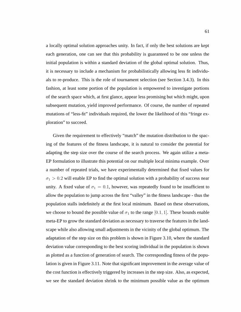
61

a locally optimal solution approaches unity. In fact, if only the best solutions are kept

each generation, one can see that this probability is guaranteed to be one unless the

initial population is within a standard deviation of the global optimal solution. Thus,

it is necessary to include a mechanism for probabilistically allowing less fit individu-

als to re-produce. This is the role of tournament selection (see Section 3.4.3). In this

fashion, at least some portion of the population is empowered to investigate portions

of the search space which, at first glance, appear less promising but which might, upon

subsequent mutation, yield improved performance. Of course, the number of repeated

mutations of “less-fit” individuals required, the lower the likelihood of this “fringe ex-

ploration” to succeed.

Given the requirement to effectively “match” the mutation distribution to the spac-

ing of the features of the fitness landscape, it is natural to consider the potential for

adapting the step size over the course of the search process. We again utilize a meta-

EP formulation to illustrate this potential on our multiple local minima example. Over

a number of repeated trials, we have experimentally determined that fixed values for

σ1 > 0.2 will enable EP to find the optimal solution with a probability of success near

unity. A fixed value of σ1 = 0.1, however, was repeatedly found to be insufficient to

allow the population to jump across the first “valley” in the fitness landscape - thus the

population stalls indefinitely at the first local minimum. Based on these observations,

we choose to bound the possible value of σ1 to the range [0.1, 1]. These bounds enable

meta-EP to grow the standard deviation as necessary to traverse the features in the land-

scape while also allowing small adjustments in the vicinity of the global optimum. The

adaptation of the step size on this problem is shown in Figure 3.10, where the standard

deviation value corresponding to the best scoring individual in the population is shown

as plotted as a function of generation of search. The corresponding fitness of the popu-

lation is given in Figure 3.11. Note that significant improvement in the average value of

the cost function is effectively triggered by increases in the step size. Also, as expected,

we see the standard deviation shrink to the minimum possible value as the optimum

62

value is approached. This effect becomes more evident as the convergence threshold is

further reduced.

0 5 10 150

0.2

0.4

0.6

0.8

1

1.2

generation, n

σ[n]

max(σ[n])

min(σ[n])

σbest

[n]

Figure 3.10: Adaptation of the standard deviation, σ1, for the 1D multisine problemusing meta-EP.

To further illustrate the dynamics of the evolution-based search, it is useful to con-

sider the same multi-sine function in two-dimensions ( = 2) in equation (3.11), shown

in Figure 3.12. We will briefly discuss the distribution of the population amidst the fit-

ness landscape (Figure 3.13(a)-(f)). As discussed, the optimal solution to this problem

is at x1 = x2 = 2π/3 = 120 as indicated by the larger (blue) circle in each figure,

where the x- and y-axis values have been converted to degrees.

Since each individual in the population now consists of a vector containing two

components, the population at a given generation can be expressed in the matrix nota-

tion:

63

0 5 10 15−4

−3

−2

−1

0

1

2

generation, n

Fitn

ess

valu

e

Best in populationAverage Fitness

optimal solution, f*

Figure 3.11: Evolution of the best individual and average fitness for the 1D multi-sineproblem using meta-EP and σmin = 0.1.

0 1 2 3 4 50 1 2 3 4 5−3

−2

−1

0

1

2

3

4

x2

x1

f(x 1,x

2)

f*(x1* ,x

2* ) = 3.5

Figure 3.12: Fitness landscape for the multi-dimensional sine function with N = 2.

64

P(n) =

x1

1 x21 · · · xµ1

x12 x2

2 · · · xµ2

(3.12)

where the initial population (n = 0) is created by associating with each individual a

pair of component values xjk, k = 1, 2 selected uniformly at random from the range

[0, 0.5]. Again, this is done so as to purposely force the evolution to explore a large

portion of the domain in order to discover the global minimum.

Mutation of the population at each generation in this case consists of applying ran-

dom perturbations to each component of the j th individual trial solution, namely:

xj+µk = xjk +G(0, σk) (3.13)

where the parameters σk serve to control the effective “step size” or move limits on

each parameter between successive generations. Note that the mutated individuals are

constrained to lie within the search domain [0, 3π/2] - if this is not done, other peaks

with the same optimal fitness value of 3.5 (due to the periodicity of the sine function)

will be found.

As the search progresses through Figure 3.13(a)-(d), the behavior can be described

as similar to “ant-like” foraging in the sense that initially a single rogue individual “dis-

covers” a fruitful region of the search space. This causes the population to generally

follow the “scent” in a cluster-like fashion. Note, however, because the “step size” is

kept constant, although a large percentage of the population clusters around the opti-

mal solution, a significant number of individuals are still “exploring” the fringes of the

domain, looking for possible alternatives. Thus, the constant variance which caused un-

desired oscillations in the simple convex case, represents a potentially desirable feature

for a problem with multiple local minima. This is a particularly attractive feature in sit-

uations involving the tracking of moving extrema. Towards this end, at generation 100,

the parameter z was changed from π/6 to π/3. This caused the landscape to suddenly

change shape, moving the optimal solution to π/3 = 6 as indicated by the new location

65

of the blue circle in Figure 3.13(e). The effect of this change in performance function

is that solutions which were previously near-optimal have now degraded considerably.

Now, the ”rogue” individuals which are spread out through various regions of the search

space suddenly increase in value in the vicinity of the new optimum. Because the ”step

size” or variance of the underlying mutation distribution has stayed constant, this allows

the population to gradually congregate around the new location (Figure 3.13(f)).

Alternatively, one might investigate the effect of scaling the standard deviation -

either according to fitness or via the meta-EP formulation. In this case, the population

is seen to group much more tightly around the global optimal solution once it is discov-

ered, ultimately converging to the point where the entire population effectively contains

the same component values. This scaling of the step size in the vicinity of an optimal

solution, however, can be a double-edged sword, depending on the desired “output” of

the search. If all that is sought is a single solution which is as close as possible to the

global optimum, then scaling of the step size can be effective. On the other hand, if one

is more interested in finding a number of “near-optimal” or “equally-near-optimal” so-

lutions, such scaling can actually be detrimental. In particular, if one is willing to accept

a certain reduction in optimality in exchange for speed of solution and the availability

of (possibly very different) alternatives, the fixed (relatively large) standard deviation

value can be desirable.

3.6 Discrete Optimization

The preceding discussion in this chapter has focused on optimization of a continuous

function of the decision variable vector. We now turn to the study of situations involving

the optimization of discrete sequences - in which the output vector consists of a string

of numbers which each take on a value selected from a finite range of integers, Imin ≤

xk ≤ Imax, k = 1, 2, . . . , . Such a representation lends itself quite naturally to a

genetic algorithm (GA)-like framework. Initially, we assume that the output decision

vectors are binary strings. The discussion is extended to the more general case of

66

0 20 40 60 80 100 120 140 160 1800

20

40

60

80

100

120

140

160

180

gen: 2

x1

y1

0 20 40 60 80 100 120 140 160 1800

20

40

60

80

100

120

140

160

180

gen: 5

x1

y1

(a) (b)

0 20 40 60 80 100 120 140 160 1800

20

40

60

80

100

120

140

160

180

gen: 10

x1

y1

0 20 40 60 80 100 120 140 160 1800

20

40

60

80

100

120

140

160

180

gen: 96

x1

y1

(c) (d)

0 20 40 60 80 100 120 140 160 1800

20

40

60

80

100

120

140

160

180

gen: 101

x1

y1

0 20 40 60 80 100 120 140 160 1800

20

40

60

80

100

120

140

160

180

gen: 160

x1

y1

(e) (f)

Figure 3.13: Illustration of distribution of population throughout space, balancing goalattraction and exploration.

67

integer strings whenever possible. In particular, following closely the development

given by Rudolph [87], we describe the asymptotic convergence behavior of this class

of evolutionary algorithms (EAs).

Recall that the optimization problem considered is the minimization of an objective

function, f(x), as given by equation (3.1). In this case, the function f maps the binary

(integer) decision vector, x, to the real numbers. Our goal is to find a discrete sequence,

x, which, when evaluated through the cost function, f(x), yields the global optimal

cost:

X∗ = x ∈ X : f(x) = f ∗ (3.14)

We assume the existence of a real-valued mapping that extracts the best objective

function value known to the evolutionary algorithm in state P(n). This sequence of

values is denoted by the random variable, B(n).

In analyzing the question of convergence for an algorithm, it is of interest to deter-

mine:

1. Is a particular EA able to find a solution of problem (3.1)? More specifically,

does the random sequence B(n) converge in some mode to the global optimum

f ∗ of the objective function? And, if so:

2. How much time is necessary to discover the solution? In other words, what is

the expectation of the random time, Tε = minn ≥ 0 : B(n) ≤ f ∗ + ε that is

necessary to solve problem (3.1) with some prescribed accuracy ε ≥ 0?

While definitive claims can be made with regard to question (1) in the general case,

theoretical results related to the expected time of convergence (question (2)) are con-

fined to special classes of functions [87]. We now explore the modeling of EAs in order

to assess the conditions under which convergence to optimal solutions can be assured.

68

3.6.1 Markov Chain Models of Evolution

As one begins to examine the nature of the process of simulated evolution, it becomes

evident that the state of the population at a given step is a function only of the state at the

previous step and the operators used to generate offspring - namely mutation and/or re-

combination and the selection process. As such, evolutionary algorithms (EAs) can be

modeled through the use of Markov chains, in which a probabilistic transition operator

maps a population P(n) at discrete time (generation) n ≥ 0 to a population P(n+ 1).

The transition operator typically consists of two parts, related to the probabilistic mod-

ification of the population (mutation and recombination) and the subsequent selection

of survivors from the modified population.

Since we model the individuals in the population as a discrete sequence of binary

numbers (integers), each selected from a finite range, the possible number of states

which the individual can take on is finite. Thus, an individual at a given generation,

x(n), can be written either in terms of its sequence values, or equivalently in terms of

its state index. For a binary string of length , we can enumerate each of the possible

states uniquely via the set i ∈ 0, 1, . . . , 2−1. We can thus define the probability that

the EA will be in each possible state at a given generation, denoted by the row vector

π[n]. Further, we define a specific transition operator, denoted by the 2 × 2 one-step

probability transition matrix, T . The entries of this matrix, τij , where i and j range

over all states of the chain, represent the probability of transitioning from state i to j

in a single step. By convention, T 0 = I , the unit matrix. For a given π[0], the product

π[0]T yields the probability of being in each state after one transition. In general, a

recursive relation can be found, namely:

69

π[1] = π[0]T

π[2] = π[1]T = π[0]T · T...

π[n] = π[0]T n (3.15)

Thus, the probability of being in each state after n such transitions, having started with

an initial probability distribution of π[0], is π[0]T n. Note that the ith row of T n is the

conditional probability mass function of x(n), given that x(0) = i. This implies that

the matrix T n is a stochastic matrix satisfying the properties:

0 ≤ τij(n) ≤ 1 and∑j

τij(n) = 1 (3.16)

3.6.2 Convergence Properties of Binary EAs

A Markov chain is said to irreducible if every state communicates with every other

state. Two states, i and j, are said to communicate if there is at least one path in the

transition diagram defining the chain from i→ j and vice versa. Note that such a path

may take multiple steps.

Note that the Markov chain defined by a GA acting on binary strings with only

cross-over and selection operators is not irreducible - there exist absorbing states (e.g.

those states that do not communicate with any others). The total number of absorbing

states (e.g. those states in which each bit string is identical) is 2, with the number of

bits used in the encoding. It can be observed that the density of absorbing states,

2

2µ= 2(1−µ) (3.17)

decreases exponentially with the length of the string, while the total number of states

increases exponentially.

70

Given these definitions, the time-varying behavior of the Markov chain can be de-

scribed (see, for example Goodman [88], Fogel [84], or Rudolph [87]) in terms of:

1. transition to an absorbing state

2. transition to a state from which there may be a transition to an absorbing state

with some non-zero probability

3. transition to a state where there is no probability of transitioning to an absorbing

state in a single step.

This process can be formalized by the definition of the state transition matrix, T ,

which satisfies:

T =

Ia 0

R Q

(3.18)

where Ia is an (a×a) identity matrix describing absorbing states,R is a (t×a) transition

submatrix describing states which may transition to an absorbing state, andQ is a (t×t)

transition sub-matrix describing states which will transition only to other transient states

and not absorbing states. As the number of transitions tends to infinity, this matrix can

be shown to take the form [88]:

limn→∞

T n =

Ia 0

(It −Q)−1R 0

(3.19)

where the existence of the inverse (It − Q)−1 is guaranteed [88]. What this implies is

that, given infinite time, the chain will transition with probability of one to an absorbing

state. Note, however, that there is a non-zero probability that the absorbing state may

not be the global best state - unless all absorbing states are globally optimal.

Essentially, the convergence results for EA can be summarized as follows for binary

search spaces (these conditions will be generalized to discrete spaces shortly). Conver-

71

gence to a globally optimal state is guaranteed, regardless of the initial distribution,

if:

1. There exists a non-zero probability of transition from any state x ∈ S to a state

y ∈ X∗.

2. The selection operator used to determine survivors from one generation to the

next always maintains the best solution found, as expressed in equation (F.3).

This requirements can be summarized by the following theorem:

Theorem 1 ([87], p119) If the transition matrix of an elitist EA is reducible and the set

of recurrent (e.g. absorbing states) is a subset of X ∗, then the EA converges completely

and in mean to the global optimum regardless of the initial distribution.

Note that it is not necessary that each state can be reached in one step. Such a

situation arises when the support of the mutation distribution is restricted to a small

neighborhood of the current position. In this case, it may be possible that the set X ∗

is not reachable from all states i ∈ S even for more than one step. Consequently, it is

necessary to impose the following condition on the structure of the transition matrix:

For each i ∈ S there exists a finite constant, no, such that the probability of reaching

the set X∗ from i in no steps is non-zero, P (no)(i, X∗) > 0. What this effectively

means is that the selection operator must be probabilistic - occasionally allowing less

fit individuals to survive to enable multiple mutation steps to transition a state to the

optimal set, X∗.

For the case where the decision vector, x, consists of a set of integers, each in the

range [0,M ], similar convergence results to those in Theorem 1 can be stated. The only

requirement is that the mutation operators chosen must enable transition between any

two integer states in a finite number of steps.

Thus, the limiting behavior of evolutionary algorithms in binary (discrete) search

spaces can be characterized by the properties of only two evolutionary operators, namely

72

mutation and selection. Other operators can be shown to have no impact on the limit be-

havior [87]. If mutation of individuals is implemented by the usual bit-flipping method

then every EA with elitist selection will converge completely and in mean to the global

optimum for arbitrary initializations. For discrete integer representations, global con-

vergence can be guaranteed assuming that mutation of individuals allows for transition-

ing between any two states in the search space in a finite number of steps.

3.7 Chapter Summary

In this chapter we provided an overview of the primary components involved in evo-

lutionary computation and discussed several particular algorithms (GA, EP) in some

detail. The performance of EP was demonstrated on both a simple convex function

and a more complex, multi-modal function with several local minima. Observations re-

garding this performance led to the obvious conclusion that the design of the mutation

operators is critical in determining the convergence of continuous EAs. In this regard,

meta-EP was discussed as a mechanism for adapting the underlying mutation distribu-

tions over the course of evolution. This is an alternative to standard fitness-proportional

scaling of the variance of the distribution.

Asymptotic convergence properties of both discrete (binary) and continuous population-

based EAs were summarized using Markov chain analysis. This analysis established

sufficient conditions for the separate variation and selection operators such that their

combination leads to a globally convergent EA in both the discrete and continuous

cases.

73

Chapter 4

PATH SPACE

In Chapter 3, we introduced the mechanism of evolutionary computation and illus-

trated its use in solving continuous function optimization problems. As alluded to in

that chapter, a key aspect of applying evolutionary computation to a given problem is

finding a population representation which lends itself well to solution of the problem.

For optimization of a continuous function, we noted that it often suffices to represent

the input search space directly in terms of the vector components of the function’s ar-

gument. We now turn our attention to the problem of describing the space of path plan-

ning. Our goal is to develop a number of different possible representations and assess

their relative strengths and weaknesses. In particular, we will focus on the matching

of mutation strategies to each of these representations and discuss the properties of

each method with regard to convergence. In doing so, we will discuss a relaxation of

convergence requirements to include not just a single globally optimal solution, but a

neighborhood of near-optimal solutions. This latter extension is essential for practical

implementation of evolution-based algorithms to the path planning problem.

4.1 Basic Concepts

For the purposes of this dissertation, we define a trajectory in space as a sequence of

physical locations of a vehicle system, each with a corresponding time. These locations

correspond to sampling of a continuous trajectory at discrete intervals of time. Each

trajectory is assumed to originate from a specified initial condition in which the vehicle

position, speed, and orientation is specified. We denote a point along such a trajectory

using the notation x[tk], where tk represents the time at which the vehicle is at position

74

x. The vector notation corresponds to the individual position coordinates, defined rela-

tive to some assumed fixed, inertial coordinate system, i.e. x[tk] = [x1[tk]x2[tk]x3[tk]]T .

An entire trajectory consists of the sequence of locations at discrete times, tk, for

k = 0, 1, . . . , N, where N is the total number of points contained in the path. In

general, the interval of time between points on the trajectory need not be constant.

Since we will be using evolutionary computation to simultaneously evolve multiple

potential trajectories for a single vehicle (e.g. within a population), it is necessary to

develop a notation to distinguish among these different trial solutions. This is accom-

plished by attaching a superscript to the trajectory corresponding to the j th individual

in the population, xj [tk]. Situations involving the coordination of multiple vehicles of-

ten required the use of multiple instantiations of evolutionary algorithms. As such, it

becomes necessary to be able to distinguish between trajectories contained in differ-

ent populations. In these situations, we add an additional superscript to denote the j th

trajectory from the ith population, namely xi,j [tk].

Since the path planning problems considered in this research nominally involve tra-

jectories defined in 4D environments (3D position, 1D time), we describe the motion of

the vehicle in terms of its speed at any time instant, u[tk] =√u2

1[tk] + u22[tk] + u2

3[tk],

its heading, ψ[tk], and its climb angle, γ[tk], as illustrated in Figure 4.1.

The components of velocity at any time instant, um[tk], are take relative to a fixed in-

ertial frame. The unit vectors for this frame are defined such that e1 points toward

the East, e2 is oriented to the North, and e3 corresponds to height above the Earth’s

surface. For ease of visualization, we generally confine the simulation examples pre-

sented to those involving only two-dimensional motion in time. This might correspond

to constant-altitude navigation, for example.

Because we often search for trajectories in a different space in which we score them,

it is necessary to develop a similar notation to represent the input search space for the

path planning problem. When multiple populations are necessary, we append a super-

script to the matrix input notation discussed in Chapter 3 (Section 3.3). Namely, P i(n)

75

e2

e1

e3

speed, u

heading angle

climbangle

Figure 4.1: The convention used in this dissertation for representing the vehicle’s 3Dmotion state in time.

denotes the ith population at generation n. We distinguish individuals in these different

populations from one another using the notation, P i,j, where i reflects the population

index and j is the individual index within the ith population. As an illustration of the

way in which individuals from different populations might be combined to coordinate

action, consider Figure 4.2. Note that the individuals are generally evolved in isolation,

yet evaluated in the same context. In this fashion, a natural separation of responsibility

is possible as each population tends to develop a distinct “niche” or specialization.

Here we see three separate vehicles, each of which is running a separate instance of

an evolutionary algorithm. In evaluating the fitness of individuals within population A,

we see that representatives from populations B and C are selected and passed into the

environment model and used to define a relative context for the actions of the individ-

uals from population A. Such a framework has been formalized by Potter [89] and is

often referred to as cooperative co-evolution. Note that the individual input representa-

76

j

+ +

evaluation ofperformance

population B

population C

population A

1 2 3 4

environmentmodel

j = 1,2,…,4

representatives

Figure 4.2: Illustration of a mechanism for combining and coordinating the action of ateam of vehicles, each represented by a separate population.

77

tions used in the contextual evaluation need not be identical.

When only a single EA is needed, the population indicator, i, is dropped - individu-

als are uniquely defined simply by the individual index, P j. Note that the interpretation

of the vector notation in the input space is more general than that of the physical tra-

jectory. The components of the j th individual, P jk are not necessarily associated with

time. Rather, we treat these components merely as sequence markers. Thus, we use

subscripts to denote these components in lieu of the square bracket notation.

4.2 Overview of Path Planning

Path planning is ultimately responsible for the generation of a trajectory in space which,

when followed, maximizes the likelihood of the vehicle completing its assigned tasks.

More formally, the types of path planning problems considered in this and subsequent

chapters can be described via the general problem statement:

Given:

• a team ofM vehicles: V1, V2, . . . , VM initially at locations x1[0], x2[0], . . . , xM [0]

respectively, each with capabilities Ci, i = 1, 2, . . .M

• a set of NT [tk] targets to be observed or attacked, T, located at positions

Ti[tk], i ∈ 1, 2, . . . , NT each with an associated value, qi[tk],

• a set of NO[tk] obstacles, O, at locations Oi[tk], i = 1, 2, . . . , NO to be

avoided,

• a set of NH [tk] threats, H, at locations Hi[tk], i = 1, 2, . . . , NH,

• a set ofNG[tk] base or goal locations, G, at locations Gi[tk], i ∈ 1, 2, . . . , NG

which the vehicles must reach in order to complete their mission, and

• a model of the terrain/environment, E(x, tk)

78

Find: a set of trajectories for each of the M vehicles, xi[tk], i = 1, 2, . . . ,M de-

fined at times k = (0, 1, . . . , N), through the set of observation or attack regions, T,

which tends to optimize a performance function, J(x1, x2, . . . , xM), subject to a set of

constraints, g(x1, x2, . . . , xM , tk) = 0.

In this problem statement, we denote the size of a set A (e.g. number of elements)

as its cardinality, or card(A). Note in particular that we distinguish between en-route

target locations and the final destination, or goal points. We also distinguish between

threats and obstacles. Threats represent features in the environment which impose a

probabilistic penalty to a vehicle traveling in their vicinity and thus can be approached

at the vehicle’s own risk. Obstacles, on the other hand, represent physical constraints

which cannot be penetrated at any cost. Detailed discussion of the formulation of threats

and obstacles for the purposes of evaluating trial paths is deferred until Chapter 5. For

now, it is sufficient to note that obstacles are appended to the cost function in the form

of a penalty term whose size is related to the degree with which a trial solution violates

the constaints imposed by their location and size.

Note that all computations are done in discrete time, where the interval ∆t is cho-

sen based on the estimate of a characteristic length and time scale of the environment of

interest relative to the vehicle speed and maneuverability envelope. This can be thought

of in terms of a Nyquist frequency in the context of discrete-time control: if the sam-

pling time is not sufficiently higher than the dynamics of interest, aliasing will occur

introducing errors in the environment representation.

We define a scenario as a particular instance of a path planning problem. In gen-

eral, a scenario need not be a static entity. Rather, the state, number, and location(s)

of each of the problem descriptors (threats, obstacles, targets, goals) can vary over the

course of a given scenario. The vehicle capabilities, Ci, target regions T, threat

regions H, and terminal locations, G, are all in general time varying and/or spa-

tially varying. For example, a threat may switch between an active and passive state or

the vehicle fuel/power levels decrease at different rates depending on the nature of the

79

trajectory. This variability includes appearance and disappearance of targets, threats,

and/or obstacles. The constraints, g(·, tk), are used to define unreachable, infeasible,

or undesirable portions of the search space. These include hard obstacles which can-

not be penetrated, vehicle performance limitations such as bounds on a vehicle’s turn

rate and/or acceleration, or prescribed minimum bounds on vehicle survivability.In gen-

eral, these constraints apply both to each individual trajectory as well as the interaction

between trajectories in situations involving multiple vehicles.

Finally, note that the performance measure, J(·), can, in general, be a complex

function over the trajectories of all M vehicles. This reflects the fact that, depending

on the nature of the mission objectives, an individual’s performance may be evaluated

in the context of other vehicles and their corresponding trajectories in space and time.

Generally, in order to facilitate evaluation of the ith path’s fitness with regard to the

performance function, including the extent to which it satisfies the constraints, it is nec-

essary to express the trajectory in the form of a sequence of physical locations in time.

This may not, however, be the best or most efficient space in which to search for tra-

jectories. Rather, it may be more desirable to search in more abstract spaces, where the

actual physical path resulting from a particular representation is then found through a

series of mathematical transformations. In what follows we discuss a number of differ-

ent ways in which the search space for the path planning problem can be represented

and highlight the relative strengths and weaknesses of each approach. It is illustrated

that the effectiveness of the different approaches depends on the degree to which a given

representation matches the requirements of the path planning problem being solved.

4.3 Path Representations

In using evolutionary programming to solve a particular planning problem, one must

first determine the way in which individuals of the population of trial solutions are to

be represented. In other words, we need to define the search space, P , consisting of

the parameters to be modified by the search process. For the purposes of path planning

80

for a single vehicle, it makes sense that a trial solution consists of a candidate path,

parameterized in some fashion to reflect variations in space, time, or both. Among the

population representations explored in this research are, in increasing order of abstrac-

tion:

• waypoint formulation (knots)

• speed/heading sequences in time

• maneuvers and transitions in time

• high-level abstract task level

These approaches can be roughly grouped into two categories: (1) a RubberBand path

description in which each trial solution by default contains the goal state and the “body”

of the path is stretched and pulled as necessary to meet the remaining objectives; and

(2) a FindGoal class of representations in which each trial path grows outward to try

and capture the goal. These two approaches are illustrated in Figures 4.3 and 4.4,

respectively. Stretching of the band connecting the start and goal points, as indicated

in Figure 4.3, involves the creation of intermediate points along the nominal band at

various points and moving these points about the free space until finding a collision-

free path. The latter FindGoal approach (Figure 4.4) requires a termination criteria,

stopping once the end point of the evolved path has reached within a certain ball of the

goal location.

4.4 Waypoint Formulation

A natural mechanism for describing a vehicle’s trajectory is through a series of way-

points. These waypoints act as a set of beacons or intermediate targets which are to be

traversed in succession. As the vehicle approaches waypoint k, the next waypoint in

81

initial location(spawn point)

obstacle

obstacle

goal

x

y

detourwaypoints

Figure 4.3: Depiction of the RubberBand class of search algorithms which attempt tostretch and pull the connecting “string” around obstacles in the environment.

initial location(spawn point)

obstacle

obstacle

goal

terminationradius

Figure 4.4: Illustration of the FindGoal class of representations in which the searchtries to discover a path to the goal by extending various branches outward.

82

the sequence, k + 1, is triggered as the active target. This process repeats until the goal

point (final waypoint) is reached.

4.4.1 Defining the Individual

Each pair of waypoints has implicitly associated with it a track segment, which is the

nominal straight-line path connecting the points. Given this simple model of navigation,

the vehicle’s trajectory in time can be suitably represented as a sequence of waypoints

and traversal speeds along each track segment. The kth point along the j th trajectory

can be expressed as:

P jk : xk, uk for k = 1, 2, . . . , j (4.1)

An entire individual consists of the vector concatenation of j such points, namely:

P j =

x1,1

x1,2

x1,3

u1

x2,1

...

xj ,3

uj

(4.2)

where the xk,m are the components of the position vector xk in either 2D or 3D space

denoting the position of the kth waypoint, and uk denotes the speed of the vehicle as it

begins motion along the kth segment. Note that time is implicit in this representation.

This is emphasized by the use of subscript as opposed to square bracket notation on the

variables.

Based on this model, the degrees of freedom which an evolutionary algorithm can

adjust correspond to (1) the number of waypoints, (2) the physical location of the com-

83

ponent values, xk,m, (3) the ordering of the waypoints, and (4) the commanded speed

along each segment. Note that the minimum number of waypoints in any given path

is 2, denoted by the set x0, which represents the initial and goal locations of the ve-

hicle. In scenarios involving a set of observation/attack targets, T, a minimum set

of additional “target” waypoints is defined such that each trial path contains at least

the target locations, xT = x : xi = Ti[tk]. If the presence of threats, obstacles,

or other features in the environment precludes the use of straight-line paths between

targets to the goal, a set of detour waypoints, xD, can be created. Thus the total

sequence of waypoints for an entire path, xP , is made up of the union of the sets of

all types of waypoints, xP = x0 ∪ xT ∪ xD. Note that the actual ordering of

the waypoints in the set xP is arbitrary except for the initial and goal positions which

are constrained to occur first and last in the sequence, respectively. The evolutionary

process attempts to discover optimal orderings with respect to a given set of mission

objectives.

In general, the speed might be allowed to vary somewhat continuously along each

track segment, although for most purposes it is sufficient to consider the traversal speed

constant along any given segment. Of course, variation of the speed along trajectory

segments must be constrained to lie within the acceleration capabilities of the vehi-

cle. The vehicle speed itself must be kept within reasonable bounds as dictated by the

vehicle’s performance envelope (e.g. to avoid low-speed stall in the case of an aircraft):

amin ≤∆u

∆t≤ amax (4.3)

umin ≤ uk ≤ umax (4.4)

Of course, in transitioning between two track segments, the rate of turn is limited by

the maneuverability of the vehicle and the bandwidth of the navigational control loop.

In situations where the distance between waypoints is large relative to the vehicle’s

effective turning radius, these effects are negligible - and a simple point mass model

84

which tracks the position of the vehicle center of mass is sufficient to model the vehicle

behavior in the environment. In general, however, depending on the spatial resolution of

the waypoints relative to the vehicle’s turning capabilities, it may be necessary to use a

more detailed dynamic model for the purpose of evaluating a given waypoint sequence,

where the model dynamics map the straight-line path defined by the waypoints into a

more detailed, approximate actual trajectory. By including an appropriate approxima-

tion of the inner and outer-loop tracking behavior of the vehicle, candidate paths can

be evaluated to ensure that they do not violate hard constraints due to drift off of the

straight-line tracks due to maneuvering bandwidth or turn rate limitations. An example

of this is illustrated below in Figure 4.5.

−500 −400 −300 −200 −100 0 100 200 300 400 500−500

−400

−300

−200

−100

0

100

200

300

400

500

obstacleS GOAL

x position

y po

sitio

n

straight−line path

modeled flight path

"knot" point

Figure 4.5: Depiction of the interaction between the navigational control loops and thewaypoint path definition.

In this example, we utilize a 2D kinematic model in conjunction with a nominal (non-

linear) tracking control law which attempts to minimize cross-track errors. As the vehi-

cle transitions between the two flight path segments, it can be observed that a significant

tracking error results due to the sudden change in heading required. This effect is ex-

85

acerbated in this case by the fact that the “active” track is not switched until after the

vehicle crosses the waypoint or “knot” point above the obstacle. More sophisticated

controller schemes may be able to better anticipate transitions between segments to

minimize transient path errors. This is similar to terrain following control, in which

look-ahead sensors are used to effectively provide “lead”, minimizing the amount of

“ballooning” over the tops of ridges [90].

4.4.2 Mutation of Waypoint Sequences

For the waypoint formulation, in which individuals are comprised of a series of way-

points and track speeds, mutation involves random perturbations applied to both the

waypoints themselves and the traversal speeds. Mutation of the j th trial solution in-

volves randomly perturbing the physical location of various points in the waypoint se-

quence:

xj+µk,m = xjk,m +G(0, σjm) for k = 1, 2, . . . , cj (4.5)

where G(0, σjm) represents a Gaussian random variable with zero mean and standard

deviation of σjm. This perturbation is applied only to c waypoints chosen at random,

where c ∈ 0, 1, . . . , j. Note that the standard deviation for each individual and along

each component direction is, in general, independent.

Other options explored for mutation include the re-ordering of waypoints and the

selective addition/deletion of waypoints. Ignoring the initial and goal locations (which

are the same in every candidate solution), the j th trajectory is given by the ordered set or

list of points, xjk, k ∈xD ∪ xT

. Reordering of this set of points is done through

the selected reversal of portions of this list of points. For example, [1 · 2 · 3 · 4 · 5] →

[1 · 4 · 3 · 2 · 5].

Exercising this formulation, and observing the nature of the best-available trajec-

tory over time, one sees that after only a small number of generations, the modification

and re-ordering of waypoints is capable of quickly discovering collision-free path that

86

connects all the target points. The optimality (e.g. length of path, mission duration,

etc.) of these early paths, however, is typically quite poor. As the evolution proceeds,

the algorithm continues to discover increasingly optimal positions and orderings of the

waypoints. Depending on the location and extent of obstacles in the environment, how-

ever, the differences in paths between simply collision-free and near-optimal trajec-

tories can be drastic. Continuous small “motion” of various waypoints may not be

sufficient. Rather, large scale changes in individuals may be necessary. This behavior

must be considered when attempting to utilize the waypoint formulation for real-time

applications. One must only re-order and adjust waypoints which do not include the

current segment and allow the algorithm sufficient time to “settle”. If not, large motion

or drastic reordering of the waypoints - although resulting in path which is more opti-

mal than the one currently being followed - will necessitate large course corrections in

order for the vehicle to transition to the new active waypoint in the sequence.

In general, the assignment of the standard deviation to each positional degree of

freedom is a major difficulty in applying this representation to different problems. At

one extreme, one can choose a large value for σjm which will allow the waypoints to

“hop” randomly around the domain. This will lead to feasible solutions, but not one

that is likely to be near-optimal. On the other hand, if one chooses too small of a fixed

variance, the “motion” of waypoints through the space due to mutation may not be

sufficient to discover collision-free straight-line trajectories. Really what is necessary

is a means to scale the standard deviation in each direction relative to the fitness. As

discussed in Chapter 3, however, this can be difficult given the uncertainty of the range

of values the fitness of paths may take on over the course of evolution. An alternative

approach would be to use the meta-EP formulation in which the standard deviations

along each dimension are allowed to evolve simultaneously with the decision vectors.

87

4.5 Instruction List Concept

Although the waypoint specification of a trajectory is efficient in terms of the size of

each individual (only requiring a minimum number of “knots” such that straight-line

travel is collision-free), it has the drawback of requiring a relatively detailed dynamic

model to ensure that candidate straight-line paths - when actually flown - do not lose

their utility. An alternative formulation is to specifically include the vehicle dynamic

constraints in the generation of trial solutions in the first place. In doing so, we can

guarantee that all candidate solutions lie within the feasible, reachable trajectory space.

Of course, this guarantee only holds when the assumed envelope limiting parameters,

such as maximum turn rate, correspond to that of the actual vehicle. If this is not

the case, as might occur in the event of some sort of damage or failure within the

vehicle system, then some sort of feedback loop is necessary between the path planning

algorithm and the navigational control laws in order to adjust the parameters according

to the actual vehicle capability.

In considering the waypoint formulation in the previous section, it becomes clear

that this waypoint sequence really serves to define a schedule of speeds and headings

(via the orientation of each track segment) in time. Transitions under this schedule

occur spatially whenever the vehicle crosses a waypoint. Generalizing this representa-

tion, one can consider modeling the vehicle trajectory instead as a sequence of speed

and heading transitions at discrete times, tk, k = 0, 1, . . . , N. We call this schedule

of transitions an instruction list and represent it through the notation, I[tk]. In situations

where the sample interval, tk+1 − tk, is constant, we can use the index notation, I[k]

to denote the instruction at a given discrete time. Starting from an initial speed and

orientation, this instruction list can be used to construct the time-varying nature of the

vehicle speed and heading over the course of the jth trajectory.

Thus, we can express the jth individual of a population in terms of a sequence of

instructions which describe the nature of the change in the motion state to be initiated

88

Table 4.1: Enumeration of the possible instructions which result in a change in motionstate when applied at each time interval, tk.

Index Speed Heading Climb Angle

1 hold hold hold

2 change hold hold

3 hold change hold

4 change change hold

5 hold hold change

6 hold change change

7 change hold change

8 change change change

at the kth time instant:

P j =

I1

I2...

I

(4.6)

where the instruction parameters, Ik, in general indicate the type of change to be initi-

ated at the kth sampling interval. In very broad terms, the set of “instructions” (possible

transitions) is listed in Table 4.1.

where each “change” is assumed to be implemented over a single interval. Note that

at this point, nothing has been said regarding how the speed and/or angles are to be

modified - this will be discussed in more detail in the following sections. As a means

of previewing the general concept, however, it suffices to associates an integer value in

the range [1, 8] to each of the possible transitions. Then, some additional perturbation

function is used to map the integer values to a corresponding change in the real-valued

speed and/or path angles.

89

Given a sequence of such transitions and defining the vehicle motion state at any

time, tk as q[tk] = u[tk], ψ[tk], γ[tk]1, we can express the sequence of vehicle state

transformations mathematically as:

q[t0]I[t0]→ q[t1]

I[t1]→ q[t2]I[t2]→ · · · I[t]→ q[t+1] (4.7)

Note that the value of the components of the motion state between sampling intervals

is, in general, not constant. Rather, the speed and heading change over each interval as

defined by the effective acceleration and turn rates initiated at the start of each interval,

as defined by the instruction. In essence, these instructions can be thought of as defining

a commanded time rate of change of the motion state, i.e. Ik ↔ qk. Recall, the only

requirement is that the vehicle motion state reaches its final value by the end of each

sample interval. Also, note that the length of the instruction list and motion sequences is

not necessarily the same. The motion state sequence will consist of at least samples.

However, depending on the fidelity (time resolution) utilized in the implementation

of each transition, the motion state sequence may contain additional samples between

those corresponding to the transition times.

Given a sequence of speeds and headings in time, as defined by an instruction list, it

is then necessary to generate a corresponding physical trajectory in space. This physical

trajectory is typically required for evaluation of the performance of a trial solution.

Depending on the relative size of the environment relative to the speed of the vehicle

and the time interval used in sampling the trajectory, the mapping used to transform

speeds and headings to physical paths can vary. For our purposes, it has generally

sufficed to assume that the action of the instruction list operators is to define constant

acceleration and turn rates over each sampling interval. In two dimensions, given a

constant acceleration, a[tk] and turn rate, ψ[tk] as defined by the transition rules above

(Table 4.1), the motion of the vehicle over an interval ∆t = tk+1 − tk, is given by the

1From this point on, we will drop the climb angle, γ[tk] from the discussion proper, with the under-standing that the operations applied to the heading angle apply to the climb angle as well.

90

equations:

x[tk+1] = x[tk]

−u[tk]ψ[tk]

(sin(ψ[tk] + ψ[tk]∆t

)− sin (ψ[tk])

)(4.8)

+a[tk]∆t

ψ[tk]sin(ψ[tk] + ψ[tk]∆t

)

+a[tk]

ψ2[tk]

(cos(ψ[tk] + ψ[tk]∆t

)− cos (ψ[tk])

)

y[tk+1] = y[tk]

−u[tk]ψ[tk]

(cos(ψ[tk] + ψ[tk]∆t

)− cos (ψ[tk])

)(4.9)

−a[tk]∆tψ[tk]

cos(ψ[tk] + ψ[tk]∆t

)

+a[tk]

ψ2[tk]

(sin(ψ[tk] + ψ[tk]∆t

)− sin (ψ[tk])

)These expressions give the exact change in the location of a point mass over the in-

terval ∆t. A caveat, however, must be given that the effective sampling time must be

sufficiently fast such that the vehicle is not allowed to pass “through” obstacles (e.g.

sample k puts the vehicle on one side of an obstacle and sample k + 1 puts the vehicle

on the other side). Under the assumptions that (1) the speed and heading sequences

are adequately bounded with respect to the physical performance limits of the vehicle

and (2) the vehicle control loops have sufficient bandwidth to track the specified speed

and heading reference trajectories, the paths generated from this integration should be

“flyable” or “drivable” (consistent with vehicle dynamics).

In situations where vehicle acceleration and turn rate capabilities are “fast” relative

to the sampling interval, a simpler kinematic model can be used. Such a model assumes

that changes in speed and heading occur instantly relative to the sample time of the

simulation:

91

x[tk+1] = x[tk] + ueff [tk] cos(γ[tk]) cos(ψ[tk])

y[tk+1] = y[tk] + ueff [tk] cos(γ[tk]) sin(ψ[tk]) (4.10)

z[tk+1] = z[tk] + ueff [tk] sin(γ[tk])

where, ueff [tk] denotes the effective inertial speed of the vehicle which may be different

from its commanded speed due to interaction with the environment. Again, the rationale

for using this simple kinematic model is the assumption of the existence of inner and

outer loop navigation control laws which enable the vehicle to track a trajectory so

long as the changes in speed and heading are constrained to lie within the vehicle’s

performance limits, defined by its capabilities vector C.

We now focus our attention on defining the nature of the change in speed and head-

ing which is called for by the instruction operators, I[tk]. In other words, we wish to

develop several mechanisms for quantifying the “how much” and “when” correspond-

ing to an instruction list.

4.5.1 Stochastic Speed/Heading Changes

We begin by reviewing and extending the basic ideas presented by Fogel in [51], in

which evolutionary programming (EP) is applied to the routing of autonomous under-

water vehicles. In this work, a set of stochastic operators is defined to realize changes in

commanded speed and heading between intervals as dictated by the instructions. Note

that Fogel did not consider acceleration of the vehicle. Rather, the vehicle’s speed and

heading was assumed to change instantaneously between sampling intervals. Further,

Fogel considered only fixed-length instruction lists, where the length of each list was de-

termined a priori and held constant throughout the evolutionary process. We relax these

assumptions by (a) considering the more general case in which constant acceleration

and turn rates are specified over sampling intervals and (b) allowing the algorithm to

adjust the number of active instructions. The discussion presented herein is limited to a

92

2D spatial dimension, such that the vehicle’s orientation is specified uniquely through a

single heading angle. The ideas presented, however, can be readily extended to include

general 3D motion of a point mass in space.

Defining the Individual

Each individual consists of a vector or list of instructions of length , where this length

is chosen based on consideration of the worst-case path anticipated through an environ-

ment in conjunction with the sampling time of the trajectory and a lower bound on the

vehicle speed. In order to define trajectories corresponding to the instruction lists within

a population, we begin with the initial vehicle position (x[t0]) and motion state (q[t0]),

assumed to be known. Each trajectory created from a given population includes this

initial state. The physical trajectory for each individual is then constructed by stepping

sequentially through the list of instructions and applying a stochastic perturbation to

speed and/or heading as defined by the instruction at each interval. For this purpose, we

represent the vehicle’s heading angle as a continuous variable, capable of taking on any

value in the range [0, 2π]. Turn rate commands at each time interval are implemented

through the addition of a Gaussian random perturbation with zero mean and adjustable

standard deviation, σψ:

∆ψ[tk] = G (0, σψ) (4.11)

where ∆ψ[tk] reflects the change in heading required over the interval from tk to tk+1.

Thus, the commanded heading at time step k + 1 is likely to be “close” to that at

time k due to the normal distribution. The variance, σ2ψ, nominally defines the spread

of possible heading turn rates. Note that the heading change requested over a given

interval (as sampled from the normal distribution) must be bounded by the maximum

vehicle turn rate, ψmax, to insure that the generated reference sequences are within the

vehicle’s performance and tracking capability:

93

ψ[tk+1] = ψ[tk] + max(−ψmax,min

(ψmax,∆ψ[k]

))(tk+1 − tk) (4.12)

Speed changes could be handled in a similar manner, by adding a normally dis-

tributed perturbation to the speed over each interval. Instead, however, we treat the

vehicle speed as a discrete variable in the range [umin ≤ u[k] ≤ umax], with a con-

stant acceleration capability of a0. As suggested by Fogel [91], commanded accelera-

tion/deceleration of the vehicle is handled through the probabilistic addition/subtraction

of a speed increment (∆u) according to:

∆u = a0

(υ − 0.5

‖υ − 0.5‖

)(tk+1 − tk) (4.13)

where υ ∼ U [0, 1] denotes a sample of a uniformly distributed random variable in

the range [0, 1]. Under this scheme, there is a 50/50 chance of increasing/decreasing

the speed in response to a “change speed” instruction. Like the commanded heading

change, the commanded speed over each interval is bounded from above and below:

u[k + 1] = max (umin,min (umax, u[k] + ∆u)) (4.14)

such that the generated reference sequence does not exceed the vehicle’s performance

envelope (e.g. low-speed stall or high-speed structural limitations).

Note that since the operators defined for the propagation of speed and heading (un-

der the direction of the instruction list) are stochastic in nature, a given sequence of in-

structions can result in the generation of an arbitrary number of different paths. In other

words, the mapping from instruction list to physical trajectory is thus one-to-many, as

illustrated in Figure 4.6. The significance of this characteristic will be discussed further

in Chapter 5 (Section 5.5.1).

94

0 5 10 15 20 25

−10

−5

0

5

10

15

x position

y po

sitio

n

Instruction List = [1 3 4 2 2 4 1 2 4 3]

initiallocation

Figure 4.6: An example of the one-to-many nature of the stochastic operators on a singleinstruction list. Each of the paths shown was generated by the application of equations(4.11) and (4.13) in response to the sequence of instructions [1, 3, 4, 2, 2, 4, 1, 2, 4, 3]

Mutation via Stochastic Changes

For the continuous speed/heading formulation, we use the same operators (equations

(4.11)-(4.13)) to mutate paths as we do to create them in the first place. For the pur-

poses of mutation, however, rather than being applied at every time step, these operators

are only applied to a subset of time steps chosen at random over the length of an indi-

vidual. Mutation of a path takes place in two phases: First, the instruction list of the i th

individual in the population is modified by selecting k instructions at random, where

k can take on any integer value in [1, 2, . . . , ]. These k instructions are then replaced

with a new instruction chosen uniformly at random from the space of all possible in-

structions. Each instruction which is replaced triggers the re-evaluation of the motion

state surrounding the kth time step. These changes in the motion state are propagated

down the length of the path (in time).

The relative change in behavior resulting from this mutation strategy hinges both on

95

the number of mutations per parent and the size of the mutations. The “size” of mutation

is effectively dictated by the variance defined on the distribution governing commanded

turn rates, upper bounded by the maximum vehicle turn rate, ψmax. Thus, significant

change in behavior or large “motion” in the path space requires the chaining together

of multiple heading variations. In some instances, perhaps the “shape” of the trajec-

tory is correct, but the time of arrival is off. In other cases, the population may have

stagnated, being distributed in a small region near a local minima. Such circumstances

lead one to consider behavior-specific mutations, effectively biasing the introduction

of new instructions toward changes in particular features of the population’s behavior.

Generally, it is desired to allow large motions when fitness is low and then to slowly

reduce the “step size” and/or number of mutations as the population nears an optimal

solution. This allows the search to quickly scan the space in a loose fashion and then

narrow in to focus on areas with the highest potential payoff relative to fitness.

Given the aforementioned structure, our population then consists of an array of

individual instruction lists, each with a corresponding sequence of speeds and headings

and a physical trajectory in space. The question now becomes whether the mutation

operators defined in terms of heading angle and vehicle speed are sufficient to solve

arbitrary path problems. A major limitation of the framework discussed so far is that it

relies on a fixed number of instructions (e.g. each individual in the population consists

of a string of integer values). A more general population representation thus includes

the probabilistic addition and deletion of instructions. This can be accomplished in one

of several fashions:

1. One can consider literally changing the length of the instruction strings for each

individual, requiring the definition of an individual-specific notation, j, to keep

track of the number of instructions contained in the j th individual. In this case,

addition of instructions is allowed up to some maximum number, max, while

deletion is allowed until the instruction list becomes empty.

96

2. An alternative approach is to instead define the baseline length of instruction list

for each individual in the population to an identical value, , representing the

maximum allowable length. Then, a NOOP instruction can be added to the list

of available instruction integers which, when present, corresponds to a skipped

instruction. This allows a variable length instruction list to be represented as

a fixed length string. The number of non-zero (or active) instructions can be

denoted by j∗.

In either case, the instruction list is given the freedom to grow and shrink as necessary

as dictated by the problem scenario.

As an example of the effect of the mutations utilized for the continuous, stochastic

speed/heading change formulation, consider the example shown in Figure 4.7 which

was constructed using 3 mutations per parent, with ∆u = 1 and σψ = 30. Here we

−20 −15 −10 −5 0 5 10 15 20 25 30

−10

0

10

20

30

40

50

x position

y po

sitio

n

prior to mutation

aftermutation

spawn point

Figure 4.7: Illustration of the effect of mutation operators for the baselinespeed/heading formulation

see several tentacles emanating from a spawn point which might represent the current

97

vehicle position. The parents are indicated by the closed dots while the corresponding

offspring paths contain open circles. For this set of mutation parameters we see that

it is quite easy to discern which offspring are created from which parents, as “like

begets like”. The “features” or quirks of a parent are preserved through the mutation

transformation while enabling the offspring to gradually explore different portions of

the search space.

4.5.2 Deterministic Speed/Heading Changes

The individual formulation in the previous section utilized stochastic operators to pro-

duce random changes in the vehicle’s motion state in response to the action of instruc-

tions. In this section, we present an alternative formulation which realizes deterministic

changes - resulting in a one-to-one mapping between instruction lists and physical tra-

jectories.

Definining the Individual

Rather than representing the vehicle’s heading at any point in time by a continuous

variable, we instead discretize the set of possible heading changes to multiples of a

fixed turn rate:

ψ[k + 1] = ψ[k] +r

Nψ

ψmax∆t for r = −Nψ, . . . , 0, . . . , Nψ (4.15)

Similarly, the possible speed variations can be expressed as:

u[k + 1] = u[k] +r

Nu

a0∆t for r = −Nu, . . . , 0, . . . , Nu (4.16)

This restriction has the effect of drastically reducing the size of the search space. At a

given point in time, the number of possible transitions is given by (2Nψ + 1)(2Nu + 1)

Over an entire sequence of instructions of length , this implies a search space of size:

98

card(S)() =∑i=1

((2Nψ + 1)(2Nu + 1))i (4.17)

In particular, we investigate in detail the case where Nψ = Nu = 1. Thus all turns

are done at the maximum possible turn rate, ψmax and all accelerations/decelerations

are done at the maximum value of a0. This corresponds to aggressive maneuvering of

the vehicle. Under this restriction, the mapping from instruction list to path becomes

one-to-one, a trajectory being uniquely defined by its instruction list. The possible

transitions, assumed to be triggered at the start of each tk, k = 0, 1, . . . , N interval in

time are thus one of:

Instruction Index

Parameter 1 2 3 4 5 6 7 8 9

∆u + − 0 − 0 + 0 + −

∆ψ − − − 0 0 0 + + +

Table 4.2: Coding of motion instructions

Note that the ordering of the transitions in Table 4.2 is arbitrary. An instruction list

of length is thus composed of a sequence of integers, each chosen from the range

[1,M ]. In order to provide for the construction of variable length paths from a fixed size

instruction list, we include a NOOP instruction with an index of 0. Such instructions

are simply skipped over in the generation of paths. Thus, the size of the search space

for an instruction list of length is (M + 1).

As an illustration of the extent to which this representation limits the reachable

space of the vehicle, consider the case where either speed or heading can change at

a given point, but not both, reducing the search space to instructions (3-7) of Table

4.2. Including the NOOP instruction, this implies a search space of size 6 for steps

forward in time. For this example, we choose = 6 resulting in 46656 possible unique

99

instruction lists. It should be noted, however, that the number of unique paths which

can be generated from an instruction list of length = 6 is less than this value, and is

given by:

card(P )() = 1 +

∑i=0

M i (4.18)

which counts all paths generated from (1, 2, . . . , decisions (in this case, 19530). This

non-uniqueness of instruction lists results due to the presence of theNOOP instruction

(i.e. the lists [3 · 0 · 4 · 3 · 3 · 5] and [0 · 3 · 4 · 3 · 3 · 5] are equivalent). Figure 4.8 shows

the reachable path space for = 5 (to keep the figure size reasonable) and the limited

instruction set (3-7). Here, the vehicle starts with at position (0, 0) with a speed of

u[0] = 2 and heading ψ[0] = 0. For this example, the fixed turn rate and accelerations

are given the values ψmax = 30deg/s and a0 = 1m/s2, respectively. The vehicle speed

is constrained to lie in the range [1, 3]. Note that evaluation of the instruction lists in

0 5 10 15−10

−8

−6

−4

−2

0

2

4

6

8

10

Figure 4.8: Enumeration of all possible paths for the limited instruction list (3-7) and = 5 for a vehicle starting at (0,0) with speed u[0] = 2 and ψ[0] = 0.

Figure 4.8 was done using equations (4.8)-(4.9), assuming ∆t = 1s and an integration

100

step size of ∆t/2 (to smooth the paths somewhat). What one concludes from Figure

4.8 is that yes, indeed, the reachable space has been reduced from the general case

in which heading is allowed to be a continuous variable. Nonetheless, the number of

unique reachable points is quite large and useful for a large number of different prob-

lem instances. Of course, the reachable space continues to grow (spatially) and become

more dense as the number of instructions, , increases. This includes the generation

of “spiral” trajectories. Generally, the fixed length of the instruction lists is conserva-

tively estimated to be on the order of the anticipated worst-case path through the space

assuming the slowest vehicle speed over each time interval.

Mutation Operators

As a means of increasing the diversity of the population over time and to allow more

extensive searching of the instruction space, we extend the mutation strategies given in

Section 4.5.1 to allow more exotic manipulation of a parent in generating its offspring.

To do so, we treat the elements of each instruction list simply as discrete items, with no

particular relationship to one another. We then adopt a number of simple list operators,

including swap(), reverse() and shift() which are each applied with a certain probability

to each individual. The action of these operators is illustrated in Figure 4.9. Currently

the application probabilities for the various operators are set to constant values, set on

the basis of experimentation, namely pswap() = pshift() = 0.25, preverse = 0.5. It is

possible that improvements could be made by adapting the probability of application of

each operator in proportion to its effectiveness at improving solutions over time (similar

to [49]). Swap() involves the literal exchange of two instructions chosen at random in

a list. Reverse() acts to flip a portion of the list “string”, whose endpoints are chosen

at random, reversing the ordering of a subset of instructions. Shift() is used to push the

items in the list in a clockwise manner, wrapping in the sense of a circular buffer. We

maintain the option of adding/deleting items to/from the end of the list as a means of

introducing new instructions. Each new instruction is “mixed” in with the other existing

101

I1 I2 I3 I4 I5 I6

I1 I4 I3 I2 I5 I6

I2 I5 I6 I1 I4 I3

I4 I1 I6 I5 I2 I3

swap(2,4)

shift(3)

reverse(4,2)

initial instruction list

Figure 4.9: Illustration of the effect of a number of discrete list operators.

items through the application of the various operators. As an illustration of the effect

of these operators, consider the representative parents and children shown in Figure

4.10. Note that it is much less obvious (as compared with Figure 4.7) which offspring

corresponds to which parent. In this case, since the biological relationships have been

noted (e.g. A− → A+) it is clear to see how features of the parent paths are “shifted”

and modified in producing offspring. Further, the relative coverage (or “step size”)

through the search space is much larger in this case than in Figure 4.7. This expanded

coverage is quite powerful in maintaining diversity of the population, thus providing

resistance to stagnation.

We have also explored the use of typical genetic algorithm (GA) operators such as

multi-point crossover and mutation (see Section 3.4.1) for the purposes of generating

offspring. An illustration of the effect of this type of variation operator is given in Figure

4.11. Here, we see the original parent (as indicated by the closed dots) along with two

offspring created through one-point crossover. The offspring are shown both before

(·)− and after (·)+ mutation. Note that in the case of offspring1, the crossover effect

102

−20 −15 −10 −5 0 5 10 15 20

0

2

4

6

8

10

12

14

16

18

20

y po

sitio

n

x position

aftermutation

prior tomutation

A+

B+

A−

B−

spawnpoint

Figure 4.10: Illustration of the “motion” through path space enabled by the discrete listmutations of swap(), reverse(), and shift().

is small compared with that of mutation. The opposite trend is true of offspring2.

The point is that this variation scheme is in general capable of both small and large

motion through the search space. This is desirable from the point of view of covering

the search space to roughly identify regions of potential benefit and then providing

localized changes in the vicinity of valuable trial solutions.

4.6 Maneuver Sequences

As a generalization of the instruction list concept, we consider representing the vehicle’s

path in terms of a sequence of maneuvers.


We presuppose the existence of a finite set of maneuver primitives, denoted by the set

M, defined for a given class of vehicles. A trajectory is then modeled as a sequence of

103

−5 0 5 10 15 20 25 30 35−10

−5

0

5

10

15

20

25

x position

y po

sitio

n

offspring1−

offspring2−

offspring1+

offspring2+

original parent

Figure 4.11: The effect of typical 1-point cross-over and mutation on trajectories. Here(∗)− denotes path after cross-over and prior to mutation while (∗)+ indicates the influ-ence of mutation with probability p = 0.1.

trajectory primitives selected from this set, ηk ∈ M, for k = 1, 2, . . . , . The set of

possible maneuvers consists of behaviors such as climb, turn right, speed up, etc. each

with an associated time interval, ∆tk, that represents the duration of each maneuver.

The jth individual in a population can thus be written in the vector form:

P j =

η1

∆t1

η2

∆t2...

η

∆t

(4.19)

By piecing together primitives and adjusting the application intervals, one can construct

104

trajectories of arbitrary complexity. For example, specifying a constant turn rate can

result in a continuum of behavior ranging from a gradual change in course for small

durations to a sustained spiral motion for large time intervals. Similar to the instruction

list formulation described previously, we assume a finite, numbered set of primitives -

which can be reference uniquely by an integer in the range [ηmin, ηmax]. For a vehicle

operating in two dimensions, a typical maneuver set might look like that shown in Table

4.3, where ηmin = 1 and ηmax = 7.

Table 4.3: Enumeration of a maneuver set for path planning in two spatial dimensions.

Index Maneuver Description

1 hold present course and heading

2 speed up

3 slow down

4 turn right quickly

5 turn left quickly

6 turn right slowly

7 turn left slowly

The application interval for each maneuver in the sequence is bounded from above, 0 ≤

∆tk ≤ ∆tmax, where the maximum bound is either chosen arbitrarily or determined

based on experience. In some cases, for example, if spiraling motion of the vehicle

may be necessary, then the maximum bound should be chosen so as to enable such a

trajectory to be easily discovered by the algorithm.

Evolution is carried out at the maneuver level, adjusting or reordering the primi-

tives and perturbing the associated time intervals. A particular maneuver can be effec-

tively removed by pulling its associated time interval to zero duration or by including

a NOOP maneuver in the setM as was done in the previous section. Of course, in

order to evaluate the fitness of a given sequence of maneuvers, an integration must be

105

performed which translates the maneuver sequence into a trajectory in time. Given the

nature of the simple motion primitives involved, however, this integration can be done

quite efficiently. In fact, equations (4.8)-(4.9) can be used, setting the time interval to

∆tk. As before, the only necessary feature required of the integration routines is that

they provide enough spatial and temporal resolution of the resulting trajectory to allow

conservative estimates of potential collisions or constraint violations to be computed.

4.6.2 Mutation Operators

The mutation operators applied to a given individual include:

• Replacing the maneuver at a given index with another selected at random from

M

• Swapping two maneuvers at arbitrary indices in the range [1, ]

• Application of a perturbation to the time interval for a given maneuver (e.g. Gaus-

sian, Poisson, etc.)

∆tj+µk = ∆tjk +G(0, σ∆t) (4.20)

• Shifting of the maneuver sequence by q units, treating the sequence like a circular

buffer, wrapping as necessary

• Reversing a sub-section of the maneuver chain, where the end points of the sec-

tion to be modified are chosen at random.

As an illustration of the effect of this set of variation operators, consider Figure 4.12

which shows two examples of mutated trajectories. A key point is that complex changes

in behavior can be enabled by the change of the maneuver index at a single time step (or

alternatively by an increase or decrease in the time interval applied to a given maneu-

ver). This is in contrast to the complex variation of neighboring instructions required

106

0 50 100 150−20

−10

0

10

20

30

40

50

x position

y po

sitio

n

path priorto mutation

path aftermutation

0 10 20 30 40 50 60 70 80−25

−20

−15

−10

−5

0

5

10

15

20

25

x position

y po

sitio

n

path priorto mutation

path aftermutation

(a) (b)

Figure 4.12: Frames (a) and (b) show two different examples of the types of variationpossible through minor changes in the maneuver sequence and the corresponding ∆tk.

to achieve the same change in behavior using the discrete instruction formulation. Of

course, the drastic changes in behavior enabled by the maneuver formulation, while

useful for quick and dirty partitioning of the search space, can tend to slow conver-

gence as a near-optimal solution is approached. The reason for this is precisely the fact

that subtle changes in trajectories are quite rare using the operators defined. In actuality,

it is necessary to “tame” the mutation operators once in the vicinity of an optimum so

as to allow more gradual variation or fine-tuning of the trajectory.

4.7 Abstract Task Level

An even higher level of abstraction is possible if one thinks of the vehicle motion plan in

terms of a sequence of locations which are to be observed or at which must be performed

some action.

107


In this case, the individual is represented by trial orderings of the various locations

and evolution takes place through perturbations on the ordering and perhaps the time

allotted to traversal between locations. At this level, one can also think in terms of

resource allocation to different tasks and make decisions about potential courses of

action based on resource depletion. Evaluation of potential action sequences in this

case involves the creation of routes through the environment, incorporating one of the

population representations described previously.

We make the assumption that the highest-level mission objective has been translated

into a set of subtasks, Ω, which are to be completed. The ordering of this tasks,

however, may not necessarily be completely defined. In general, the definition of a

particular subtask, si ∈ Ω will require the following:

1. dependencies

si → sk for some k ∈ Ω (4.21)

si ← sl for some l ∈ Ω (4.22)

(4.23)

where the notation ()→ () and ()← () is meant to imply forward and backward

dependencies, respectively. In other words, the ith subtask may require a certain

subset of Ω to be completed prior to and after its execution. These pre/post-

requisities impose partial ordering constraints on the optimization process.

2. relative priority: denoted by pi, to be used for resolving conflicts or deleting

excessively difficult to reach/accomplish objectives. For this purpose, we assume

that the priorities for each sub-task in a chain sum to unity,∑pi = 1.0.

3. time constraints: on arrival at a given subtask, in general expressed in terms of

108

an upper and lower bound (time window) in which arrival is acceptable:

til ≤ tivisit ≤ tiu (4.24)

where, in the two extremes, if there is no time constraint, tl → 0, tl → inf and

if there is a single point time constraint (e.g. for coordinated arrival at a given

location), then tl → ti∗, tu → ti∗.

4. time duration: required to accomplish a given subtask. We express this as a nom-

inal value plus a perturbation which may either be random or driven/correlated

by environment or vehicle state:

∆i = ∆nominal + ε∆ (4.25)

5. resource drain/utilization: required to accomplish a given. Again, we model as

an expected nominal drain and random deviation:

ri+

k = ri−k + ∆rnominal

+ εr (4.26)

for each of the resources, rk, assigned to this subtask, where the ()+ and ()−

reflect the predicted resource level prior to and after completion of the task.

In constructing a plan or strategy for accomplishing a given high-level mission objec-

tive, we have at our disposal a set of resources, denoted by ri. Such resources might

include:

• fuel

• battery/power

• memory

• communication bandwidth

109

• camera/sensors

• weapons (offensive/defensive)

• radar/proximity sensors

Note that the resource expenditure is typically a function of the nature of the tasks

and may depend on the order in which tasks are completed or the state of the vehi-

cle/environment when the task is initiated. For example, battery power usage is related

to the number and type of devices and the duration of activity. Communication re-

quirements might draw on internal resources such as power as well as “external” shared

resources including bandwidth. Even still, line-of-sight restrictions may force path de-

viations to conform to visibility and range requirements for reliable data transfer.

4.7.2 Mutation Operators

Operators similar to those developed for the maneuver sequence could be applied to the

abstract task-level representation as well.

4.8 Comparison Between Different Representations

This section describes the various mutation operators which are applied to the parents of

the different representations in order to create offspring. The necessary feature of both

the population representation and the mutation strategies is that they are chosen such

that they can encode any possible configuration in the associated search space. Further,

it must be possible to move from a given configuration to any other configuration in

a finite number of mutations (see Chapter 3). In other words, to avoid being trapped

in local minima, the mutation operators must be sufficiently rich to move relatively

“large” distances in the state space. In situations where the solution is close to optimal,

the offspring should be quite similar to the parents, exhibiting only minor variations. On

the other hand, if a given parent is far from optimal, then a larger perturbation should be

110

applied. This is the idea behind fitness proportional adaptation of the distributions used

for mutation. Of course, care must be taken such that the search does not prematurely

lock on to a local minima which fails to satisfy the primary mission objectives. The

alleviation of such phenomena will be discussed in more detail in Chapter 5.

4.9 Summary

In this chapter, we detailed several different ways in which the “input” space of path

planning can be represented. The waypoint formulation, in which the algorithm searches

for a collision-free straight-line path connecting the start point through any targets to

the goal is useful for providing a general feel of the “free” space in the environment.

The shortcoming of this approach stems from the difficulty in setting appropriate stan-

dard deviations for the mutation distributions of each degree of freedom, particularly as

the distribution of threats or obstacles in the environment changes in time. Further, al-

though creation of intermediate “detour” points potentially gives this approach a bit of

flexibility in routing the vehicle, this formulation is generally limited to finding straight

paths between each “knot’ point. Nonetheless, this technique can prove useful in situa-

tions where the detail of travel between waypoints can be left to a reactive navigator.

We then presented a FindGoal class of algorithms, including a continuous (stochas-

tic) and discrete instruction list concept. The continuous representation is the most

general as it allows the heading (and turn rates) to vary continuously over the valid

range. However, as pointed out, the stochastic nature of the operators used to realize

this representation make the mapping from instruction list to trajectory one-to-many.

Although we will discuss the impact of this further in the next chapter, it suffices for

now to mention that this non-uniqueness makes it difficult to associate changes in the

instruction list with corresponding changes in the trajectories. As an alternative, we

thus present a discrete version in which the changes in speed and heading are fixed at

constant values. In this manner, the mapping from instruction list becomes one-to-one.

Thus, changes in the instruction list have a direct impact and relation to the correspond-

111

ing physical trajectory.

Finally, we described a generalization of the instruction list concept in which each

trial trajectory is generated by the piecing together of trajectory primitives, chosen from

a finite set of available maneuvers. It was demonstrated that this representation has

the desirable property that complex changes in trajectory can be introduced by very

localized changes in the maneuver sequence. Thus, one does not need to rely on the

simultaneously mutation of many sequential instructions in order to introduce dramatic

changes in behavior. As expected, however, this quality comes at the expense of the

ability to introduce minor alterations and to fine-tune solutions as one approaches near-

optimality. Thus, it may be desirable to consider changing the nature of the mutation

operators depending on the progress of the search. For example, once within a ball of

a given radius from the desired state, perhaps mutations should consist only of time

perturbations as opposed to variations in manuever indices over the length of each trial

solution.

Alternatively, one could conceivably utilize a hybrid individual representation, wherein

the interpretation of the values in the input vector changes in time according to the

progress of the search and the state of the environment. Early on in the search, the val-

ues might denote the location of waypoints, roughing out the free space connectivity.

Then, perhaps the waypoints might be connected to the extent possible given the dis-

tribution of obstacles using a maneuver sequence formulation. Finally, minor tweaks

and adjustments could be done by selectively modeling trajectories at different points in

space and time using the discrete or stochastic instruction list formulation. Taking this

idea a step further, the actual values contained in the input vectors could even vary over

the length of a given individual as well as between individuals. Dynamically adapting

the form of the input vector over the course of the evolutionary search would allow

small, detailed changes in “tight” areas of the search space and larger changes in the

more unconstrained regions. This would likely improve the efficiency during the latter

portions of the search.

112

Chapter 5

EVALUATION OF PERFORMANCE

In Chapter 4, we enumerated several different techniques for representing the in-

put space of trajectories and the ways in which these representations can be evolved.

In this chapter, we address the problem of assigning a score or fitness to each of the

candidate solutions in a population, given that they have been transformed based on

the vehicle dynamics to physical trajectories. This score is the basis for the selection

process at the root of simulated evolution. We also discuss the uniqueness of solutions

to path planning (or lack thereof) and introduce the notion of optimalizing as a desired

characteristic. Finally, we describe a common problem in optimization, namely that

of local minima. We illustrate when and why such phenomena arise in the context of

path planning and explore some mechanisms for avoiding being trapped by these local

minima.

5.1 Overview

Ultimately, the fitness of individuals within a population must be determined as the

basis of the natural selection process (see Section 3.4.3). Recall that we wish to cast

the path planning problem as an equivalent minimization problem. This requires the

definition of an objective function which reflects the suitability of a given trial solution

for survival within a particular environment. This includes specification of performance

measures not only related to satisfaction of mission objectives (e.g. positive reinforce-

ment) but measures related to the extent to which a given trial path violates certain

constraints. Such constraints may be imposed by the mission specification, the environ-

ment, or the vehicle itself. As such, the objective function must capture all the forces

113

which conspire to derail the intentions of the vehicle. For example, a typical environ-

ment may consist of forces which directly affect the motion of the vehicle (e.g. wind or

terrain variations), fixed or moving obstacles which must be avoided, active adversaries

which are trying to hide, etc.

In general, the performance measure can range from a simple scalar value to a

complex, multi-objective vector evaluation. Its complexity can range from a closed-

form algebraic solution to a full-blown non-linear simulation of the vehicle interacting

with its environment, depending on the fidelity requirements and the features of the

environment with which the vehicle is interacting. For the purposes of evolution-based

path planning, it is important to develop an efficient computational scheme to determine

the extent to which an arbitrary solution (a) satisfies constraints and (b) meets the stated

objectives. Efficiency is critical due to the “generate and test” nature of evolution-

based search in which the cost function is evaluated a large number of times. In fact,

typically, the cost function evaluation takes up a significant percentage of the overall

computational loading associated with the application of simulated evolution.

5.2 Cost Function Definition

Independent of the representation used to model individuals in the population, evalua-

tion of individuals requires a mapping from the input space of decision vectors to the

output space of performance. For the path planning problem considered here, trans-

formation from the input space (the space within which evolution occurs) to the per-

formance space (the fitness of a path) involves representation of each individual in the

population in terms of its corresponding physical trajectory. Thus, prior to evaluating

the cost of a given path, we first transform its representation to an equivalent form con-

sisting of a sequence of positions in time, x[tk], where, the time index is assumed to

take on values in the range k = 0, 1, . . . , N j . Here, N j represents the number of points

in the jth physical trajectory resulting from the integration of the input representation

(of length ) forward in time. In general, the number of points in the physical path,

114

N j , is greater than or equal to the number of active components of the input vector, j ,

depending on the temporal resolution of the output path relative to the input vector. For

example, the discrete instruction list formulation will produce paths of length N j ≥ j∗,

where j∗ is the number of non-zero instructions in the j th trial instruction list.

Once a path has been created, it remains to evaluate the physical trajectory in the

context of the various components of cost. Thus, the entire mapping from input space

to output space can be expressed as:

P j Γ(P j)→ xj [tk]J(xj [tk])→ f j (5.1)

where Γ(P j) represents the intermediate mapping from the input space to the physical

trajectory space. This trajectory represents a sampled version of a continuous trajec-

tory, where the sample points in time are defined by the tk for k = 0, 1, . . . , N j. As

mentioned in Chapter 4, this intermediate mapping may not be one-to-one, depending

on the population representation used. The performance function, J(xj [tk]), in general,

can consist of an arbitrary number of components corresponding to different objectives.

In situations involving the coordination of action amongst multiple vehicles, the perfor-

mance components may require the evaluation of multiple paths simultaneously. Thus,

given a total of M vehicles, represented by the set V , each individual in the ith popu-

lation, xi,j must be evaluated in the context of representatives selected from the other

M − 1 populations, xs,r for s ∈ V | s = i. The representatives, denoted by the

individual index, r, are chosen based on some measure - generally the best performing

individual available in each population.

5.3 A Scalar Cost Function

The simplest form for the mapping from physical trajectory to performance space is

through a scalar cost index, J(xj)→ f j. To include the effect of multiple objectives, a

penalty function approach is used in which the cost of a path is equal to the weighted

sum of the various cost components:

115

f j(w, xj) =F∑k=1

wiJi(xj) (5.2)

where w ∈ RF is the vector of weights applied to each component of cost and F is the

total number of different components. This formulation requires each objective to be

cast in the form of a “penalty” to be minimized. The basic performance components

which we consider in this research include:

1. Distance from the terminal point on a path for the ith vehicle to its goal location,

Gi[tNj ] : RangeGoal. The termination time at the goal location, tNj may be

either be explicitly specified (tNj = ti∗) or left as a free parameter.

2. Distance of closest approach between a path and any targets associated with that

path : RangeTargets. Again, time-of-arrival constraints can be introducing by

computing the distance of approach at specified times, tas , for any of the s ≤

NT [tk] targets.

3. A measure of the degree to which a given trial path penetrates the set of NO[tk]

known obstacles : ObstaclePenetrate

4. The energy (power and/or fuel) utilization along a given trajectory (including

minimum acceptable reserve values) : EnergyUsed

5. The reduction in the probability that a vehicle will survive to a given instant of

time as a consequence of interaction with threats (including a minimum accept-

able survival value): SurvivalProbability

6. The cumulative change in angle over the length of the path : PathAngle

7. The cumulative length of each path : PathLength

116

The first three of these performance measures can be directly expressed as penalty terms

as their ideal value is zero in each case. The latter components, however, can require

greater creativity in order for them to have the desired effect on the evolution of paths.

5.3.1 Computation of Cost Components

In reading through the sections which follow, it is useful to refer to a visual example of

the nature of several of the predominant contributors to the performance of a trial path.

Shown in Figure 5.1 are RangeGoal, ObstaclePenetrate, and RangeTargets.

RangeGoal(P1)

RangeGoal(P2)

RangeGoal(PM)RangeTarget(PM)

obstacles

GOAL

TARGET

ObstaclePenetrate()

Figure 5.1: Overview of cost computation.

Now, each of the cost components will be described in more detail.

RangeGoal and RangeTargets

The computation of the RangeGoal and RangeTargets components of cost is rela-

tively straightforward. We define the function R(u,v) as the Euclidean distance be-

tween two points in u,v ∈ RD, where D represents the number of components needed

117

to specify positions in the domain of interest. Thus,RangeGoal is simply the Euclidean

distance measured between the final point on a given trajectory and the goal location:

RangeGoal = R(xi,j[tNj ], Gi[tNj ]

)(5.3)

The RangeTargets cost is computed by finding the minimum Euclidean distance be-

tween the jth path (evaluated at each point xj [tq], q = 1, 2, . . . , N j) and the set of

targets, Ti, associated with the ith vehicle:

RangeTargets =∑s∈Ti

minqR(xi,j[tq], Ts) (5.4)

ObstaclePenetrate

For the purposes of this research, it is assumed that obstacles in the environment can

be suitably approximated by circular (in 2D) or spherical (in 3D) regions. Thus, ob-

stacles are defined by their time-varying center position, Oi[tk], and diameter, Di[tk],

for i ∈ 1, 2, . . . , NO[tk]. Obstacle penetration is computed using the concept of the

minimally enclosing rectangle (MER), as illustrated in Figure 5.2 below.

At a zero-th order of accuracy, the vehicle position at time tk can be compared with

that of each of the other vehicles and obstacles present in the scenario. Assuming that

the vehicle and obstacles can be suitably approximated by a set of rectangular bounding

boxes (oriented with the coordinate axes), relatively efficient collision detection can be

done by computing the overlap between any two rectangles at each time step. The

penetration penalty over the entire length of the j th path can then be expressed as the

summation of the (possibly scaled) overlap areas computed for each time step tk, k =

0, 1, . . . , N j. Depending on the vehicle speed relative to the size of the obstacles in

the environment and the sampling time used to represent trial solutions, however, this

brute force technique can “miss” collisions. Such a case is depicted in Figure 5.2.

A slight improvement can be made by modeling the vehicle as a disk (sphere) of

radius, Rvehicle, and considering its motion along a particular path segment from time

118

vehicleposn t k+1

vehicleposn t k

vehicleposn t k-1 fixed

obstacle

movingobstacle

tk-1

tk

tk+1

Figure 5.2: Illustration of basic collision detection based on the intersection of mini-mally enclosing rectangles

tk to tk+1, as shown in Figure 5.3.

We approximate the area (volume) swept out by the vehicle over this time interval

by the rectangle shown. An assumption is made that the obstacle rate of motion is slow

relative to that of the vehicle such that it cannot “jump” over the vehicle MER in the

time interval tk+1 − tk. Rather, in order to pass to the other side of the vehicle MER,

the obstacle MER must overlap that of the vehicle. In this fashion, we not only check

for collisions at the end points of the segment but also along the length of the segment.

A more exact collision detection model scheme would model the motion of both

the vehicles and obstacles using bounding rectangles to capture their movement over

each sample interval. Collision detection would then involve checking for the inter-

section of each possible pair of rectangles (each at potentially arbitrary orientations).

Such a detailed computation is outside the scope of the current research. Other gen-

eralized collision detection algorithms are available in the literature for this purpose,

many with their origin in computation of penetration of surfaces in haptic rendering

119

RvehicleRo

obstacle position attime tk

x[k+1]

x[k]

path-boundingrectangle

obstacle-boundingrectangle

Figure 5.3: Illustration of collision detection assuming that obstacle motion is insignif-icant between sampling instants

of virtual environments [92]. Many of these algorithms involve the tracking of “clos-

est features” between each pair of objects (e.g. [93], where each object is modeled

as a convex polyhedron. Work by Kim [94] models each object as spheres. Other

approaches include I-Collide [95], which exploits coherence (in time and space) be-

tween subsequent action frames as well as various hierarchical bounding-box tech-

niques (e.g. [96]). A detailed summary of the various algorithms available is provided

at http://www.stanford.edu/ jgao/collision-detection.html.

EnergyUsed

In the simplest case, we model the energy utilization as proportional to the square of

the vehicle speed at any instant - thus the total energy expenditure over a path is given

by:

∆E = E0 − Ef = cNj−1∑k=0

u[k]2 (5.5)

120

which effectively penalizes the vehicle for generating trajectories with higher speeds.

To better reflect the fact that fuel efficiency can vary as a function of speed, a slightly

different model can be used:

∆E =

Nj−1∑k=0

(∆Emin + c (u[k]− uopt)2) (5.6)

which has the effect of encouraging the vehicle to generate paths where the speed hov-

ers around the fuel-optimal speed, uopt. This optimal speed can vary as a function of

the vehicle’s location in the environment (e.g. due to effects such as terrain variations,

winds, or altitude). The model for energy utilization can be made as detailed and ac-

curate as needed, depending on the requirements of the mission being planned. For

example, it may be necessary to develop a high fidelity model of the vehicle engine in

cases where fuel flow varies as a complex function of the vehicle state, particularly in

cases where range or endurance-optimal flight is desired.

In situations where a minimum reserve is required at the end of the mission, an

additional penalty related to the extent to which any path violates this reserve value can

be added. One way in which such a consideration can be built into the cost function is

through an expression of the form:

∆J = Ef required −Ejf (5.7)

where Ef required represents the minimum acceptable reserve value. Thus, trial solutions

with final reserve values which exceed this minimum threshold contribute a negative

cost increment and are thus encouraged. Note that in evaluating a given trial solution,

the vehicle is effectively “stopped” at the location and point in time at which it exceeds

the reserve threshold. Thus, any instructions which take place after the vehicle “runs

out of gas” are ignored and all calculations involving range to various targets and goal

locations are done using this “out of gas” location.

121

SurvivalProbability

While obstacles are treated as hard constraints, threats are considered as entities which

have associated with them a certain degradation of survival probability. The model of

threat interaction is related to both “how close” a vehicle gets to a given threat as well

as the duration of time the vehicle spends in its vicinity. Thus, threats can be inter-

preted in the context of “radar” sites which might guide, for example, the deployment

of anti-aircraft weaponry. For our purposes, we equate detection to the probability of

the vehicle being “killed” or otherwise decapacitated. Mathematically, this is expressed

in terms of a probability of detection at any instant of time, Pd[tk], given by:

Pd[tk] =∑q∈H

1

1 + a[tk]R(xj [tk], Hq[tk]

) (5.8)

which is parameterized by a time-varying lethality parameter, a[tk]. When a threat is

active, this parameter takes on a value∞ a[tk] ≥ 0. An inactive threat is modeled

by letting this parameter take on the value a[tk]→∞ which effectively sets the proba-

bility of detection to zero. Of course, this detection model can be made more complex

by including an effective maximum range of detection as well as incorporating a depen-

dence on vehicle velocity and/or orientation relative to the radar site. The probability

of survival at any given instant, tk, is equal to the probability of survival at time tk−1

times the probability of not being detected at tk:

Ps[tk] = (1− Pd[tk])Ps[tk−1] (5.9)

Although in the research presented here we have restricted our attention to the simple

model above, in general, the vehicle’s survival can depend on other factors including a

more complex model of probabilistic battle damage resulting from interaction with both

stationary and active threats in the environment. This leads one to the consideration of

“battle dynamics” models such as that presented in [97].

122

PathLength and PathAngle

As one considers ways to guide the planner toward the discovery of shorter paths, the

first and most obvious choice is to try and limit the number of points in the path. More

specifically, one can try to minimize the PathLength, which can be expressed mathe-

matically as:

PathLength =

Nj−1∑k=0

uk (tk+1 − tk) (5.10)

It thus would seem natural to include a term proportional to PathLength in the scalar

cost function. Depending on the relative weighting applied to this term, however, often

times the algorithm determines that the best solution is for the vehicle to not move at all,

PathLength → 0. Obviously this is not the desired behavior. This is also a problem

in general whenever the path must grow in order to reach the target. Depending on

the relative reduction in RangeGoal, for example, as compared with the increase in

PathLength, the extension of a path may actually be discouraged - even though it puts

the endpoint closer to the goal. Thus, care must be taken in establishing the weights of

the various terms contributing to the cost.

An alternative formulation is to refer to the adage that the “shortest distance between

two points is a straight line”, introducing a term proportional to the PathAngle,

PathAngle =

Nj−1∑k=0

(ψ[k + 1]− ψ[k]) (5.11)

to the cost function. In this fashion, shorter paths are generally preferred. The effect

of such a penalty on the evolved trajectory is shown in Figure 5.4. Here, the left-

most trajectory (Figure 5.4(a)) is obtained with the weight on PathAngle set to zero.

Although the path reaches the goal location, it exhibits considerable zig-zags along

its length. When this weight is given a small positive value (0.1), the considerably

straighter trajectory shown in Figure 5.4 is obtained.

Obviously a performance component conflict, similar to that described in the discussion

123

−20 −15 −10 −5 0 5 10 15 20−20

−15

−10

−5

0

5

10

15

20

S

GOAL

Range to targets:

Range to goal:

Energy value:

0.52345

0

502

mode:

gen:

0

13

C

x position

y po

sitio

n

−20 −15 −10 −5 0 5 10 15 20−20

−15

−10

−5

0

5

10

15

20

S

GOAL

Range to targets:

Range to goal:

Energy value:

0.66634

0

518

mode:

gen:

0

39

C

x position

y po

sitio

n

(a) (b)

Figure 5.4: Simple A to B planning example (a) with no path angle penalty and (b) withadditional penalty on path angle deviations.

of PathLength, can occur in situations where the vehicle must turn from its current

course in order to reach the goal. Again, such conflicts arise due to the fact that as one

cost is decreasing, others can be increasing. The net change in cost resulting from the

change in heading in conjunction with reduction in distance to the goal must be negative

in order for such a mutation to be promoted to survival. If the population happens to

consist of the set of all paths which reach the goal, then it is a simple matter to select

the one (based on its cost component value, PathAngle) which is “straightest”. More

typically, however, it will be necessary for the EA to generate (via mutation) a path

which is straighter and reaches the goal. The likelihood of such an event can vary

depending on the other constraints (e.g. distribution of obstacles) in the environment.

5.3.2 Combining Cost Components

Having defined the various cost components, we now focus on the effect of summing

these together to produce a single scalar cost function in the form of equation (5.2). To

do so, we walk through a simple example involving a single vehicle in which all possible

124

input vectors in the search space, P , are assumed present in the population. Essentially

we are modeling the scoring of the entire population, P over a single generation. This

is obviously a contrived case, but is useful for the purposes of illustration.

We enumerate this set of paths through an exhaustive search of the path space. For

the purposes of this illustration, we assume that the input vectors take the form of dis-

crete instruction lists and use the deterministic speed/heading change formulation to

construct the corresponding physical trajectories. We take the available instructions at

each decision step to be those labeled (3-7) in Table 4.2. Thus the instruction at any

time step can take on six unique values, including the ‘0’ or NOOP instruction. As a

reminder, this subset of instructions represents changes in speed or heading at a given

time step, but not both. Our objective is to find a path consisting of at most = 6 future

decisions which reaches from the starting location x[t0] = (0, 0) to the goal location

G = (10, 0). Recall that the total size of this space is card(P) = (6) = 46656.

However, because of the availability of the NOOP instruction, the actual number

of unique paths which can be generated from this set of instruction lists is given by

card(P∗) =∑

i=0(6)i = 19531. We will consider only this set of unique paths in the

subsequent discussion.

The vehicle is assumed to be initially located at the starting point x[0] = (0, 0) with

a speed, u[t0] = 2 and a heading of ψ[t0] = 0. Speed changes are limited to ∆u = ±1

with the vehicle speed constrained to be an integer in the range [1, 3]. Heading changes

are limited to ∆ψ = ±30. The environment through which the vehicle must navigate

consists of four obstacles, NO = 4, located at the positions indicated in Figure 5.5.

The location of these obstacles is assumed constant. Two of these obstacles are also

modeled as threats in the form of active radar sites. The probability of radar detecting

(and thus potentially killing) the vehicle is modeled by equation (5.8) with the threat

lethality parameter, a[tk] = 50, a constant. Our intention in this example is to illustrate

the way in which the various cost function components effectively “filter out” different

portions of the population.

125

At a minimum, we require the search algorithm to yield feasible paths - i.e. those

which at least satisfy the constraints. This implies that the paths delivered by the planner

do not penetrate the set of obstacles. Thus, the first component of cost we consider can

be written:

J1

(xj)

= w1ObstaclePenetrate(xj , O) (5.12)

where we take the scaling parameter, w1, to have the value w1 = 1000. Since we really

are only interested in solutions which have J1 ≡ 0, this scaling is strictly not necessary

- a simple binary value would suffice. However, recall that in general, this will not be

the only component of cost. Because we scale the ObstaclePenetrate value based on

the area of overlap between the trajectory and the obstacles, this scaling factor prevents

the algorithm from accepting solutions which partially penetrate obstacles yet reach

close to the goal in situations where RangeGoal is included in the cost formulation.

Applying this cost function to the space, P , and throwing out any paths which return a

non-zero value for J1, we are left with the set PO− ⊆ P , as depicted in Figure 5.5.

Recall that the speed/heading formulation falls into the FindGoal (see Chapter 4)

class of search methods in that the goal is not explicitly included in each trial path

by default. Rather, the search over sequences of motion decisions is aimed first and

foremost at “discovering” the subset of trajectories which are collision-free and that

connect the vehicle initial location to the goal location. Thus we wish to search the

space of collision-free paths, PO−, to find the set of paths which reach close to the goal.

The simplest cost function to be used is thus concerned with minimizing the distance

between the end point of the jth trial solution and the goal, which can be expressed as:

J2(xj) = J1(x

j) + w2RangeGoal(xj [tNj ], G[tNj ]

)(5.13)

where the function RangeGoal denotes the range or distance between the end point of

the path and the goal location. Recall that we assume the path xj [tk] corresponding to

the instruction list, Ij is of length N j ≥ j , with j representing the number of active

126

−2 0 2 4 6 8 10 12 14 16 18−15

−10

−5

0

5

10

15

1

2

34

x position

y po

sitio

n

start

goal

radarsites

obstacles

Figure 5.5: Display of the subset of paths, P O−, which are collision-free. Note thatthe number of unique instruction lists represented in this set is 7177 or 37% of the“population”.

instructions. Obviously the ideal value of this cost function is J2(·) = 0. For our

purposes, however, we define a path to be “close enough” if its endpoint falls within a

ball of unit radius, resulting in J2(·) ≤ 1. The distribution of range error over the set of

collision-free paths is shown in Figure 5.6(a), for the original ordering of paths (from

the exhaustive search) and in Figure 5.6(b) where the paths have been sorted in order of

increasing RangeGoal values.

Applying this condition to the subset of collision-free paths results in the discovery

of the set of paths which are collision-free and extend to within a ball of unit radius

of the goal location, denoted by PGO− ⊆ PO− ⊆ P . For this example, this set is of

size card(PGO−) = 28, and is shown in Figure 5.7. Note that the number of visibly

distinct paths appears fewer since the end points of the “shorter” paths penetrating the

goal region are overlapped by the longer paths.

At this point, we have identified the set of collision-free paths which meet the ter-

127

0 1000 2000 3000 4000 5000 6000 7000 8000−2

0

2

4

6

8

10

12

14

16

path index [s*]

Ran

geG

oal[s

* ]

acceptance threshold

over all obstacle free paths

0 1000 2000 3000 4000 5000 6000 70000

5

10

15

path index, [i*]

Ran

geG

oal[i

* ]

0 50 1000

0.5

1

1.5

2

path index, [i*]

Ran

geG

oal[i

* ]

acceptance threshold

over all obstacle free paths

(a) (b)

Figure 5.6: Variation in RangeGoal over the set P O− of collision-free paths over theoriginal indices, i and those sorted on the basis of increasing RangeGoal, i∗.

0 2 4 6 8 10 12−3

−2

−1

0

1

2

3

4

5

1

2

3

4

x position

y po

sitio

n

Ps = 0.74

Ps = 0.52

radar sites

obstacles

goal region

start

Figure 5.7: Display of the subset of paths, PGO−, which are collision-free and extendto within a ball of unit radius of the goal location. Note that the number of instructionlists represented in this set is 28 or 0.14% of the total “population”.

128

mination criteria. It is conceivable that one might wish, in addition, to maximize the

vehicle’s probability of survival upon reaching the goal location. Thus, we desire to

discover a route within the subset of collision-free and goal-reaching paths which has

associated with it a large probability of survival. If we were actually searching for such

a route, as would typically the case outside of this contrived example, we could add a

term to the cost function to encourage discovery of such routes. Since we are trying to

minimize the scalar cost index, however, we must add this term either in an “inverse”

fashion, such as:

J3(xj) = J2(x

j) +w3

Ps[tNj ](5.14)

or alternatively, in the form:

J3(xj) = J2(x

j) + w3

(Psrequired − Ps[tNj ]

)(5.15)

which has a similar effect of encouraging survival probabilities that are greater than or

equal to the minimum acceptable survival level. For this example, we utilize equation

(5.14) and take the weighting parameter, w3, to have the value w3 = 100. We can plot

the distribution of the function J3(·) over the unique path space, P∗, as shown in Figure

5.8.

Here we have used a log10 scale on the vertical axis to allow the different cost compo-

nents to be identified. This is the cost function that the EA would “see” as it carried out

an actual search. Note in particular that the ObstaclePenetrate component, due to the

scaling w1 = 1000, dominates the cost over the set of colliding paths, PO+. At the left

of the figure, we see that the SurvivalProbability and RangeGoal dominate the cost

over the collision-free set, PO−, as would be expected. Thus, it is relatively easy for the

EA to quickly find feasible (collision-free) solutions. It is the focused search within this

collision-free subset required to satisfy additional constraints and/or objectives which

can be difficult depending on the particular problem of interest.

129

0 0.2 0.4 0.6 0.8 1 1.2 1.4 1.6 1.8 2

x 104

1

2

3

4

5

6

7

path index, i*

log 10

( J 1[i* ] )

ObstaclePenetrate

RangeGoal + 100/SurvivalProbability

Figure 5.8: Distribution of the cost function J3(xj) over all paths j ∈ P∗ (the unique

path set).

Confining our attention to only the setPGO−, we have the distribution of SurvivalProbability

given in Figure 5.9 along with the unsorted RangeGoal values.

From this figure one can observe different “pockets” of paths with essentially the same

SurvivalProbability. Thus, for a given approximate value of survival, a large number

of different paths, each satisfying RangeGoal(·) < 1 could be chosen. Paths having

the highest and lowest survival probability are indicated in Figure 5.7.

5.4 Paths, Not Necessarily Unique

As indicated by the various plots in the previous section, there are often times where

many paths can be generated with essentially the same fitness values. Thus, one is

left with making some sort of value judgement to pick a particular solution over others

which are “close” in terms of cost. Often times, however, solutions which are similar

in cost are actually quite “far” in terms of their potential for ultimately meeting the

130

0 5 10 15 20 25 300

0.1

0.2

0.3

0.4

0.5

0.6

0.7

0.8

0.9

1

path index [i*]

Cos

t Com

pone

nts

for obstacle free paths satisfying RangeGoal < 1

Figure 5.9: Distribution of the probability of survival at time tN over all paths i ∈PGO−.

objectives of the mission. This is particularly true as one is assessing trial solutions

over a limited planning horizon - one that does not necessarily stretch (in space and

time) all the way to the terminal state.

When performing search in an arbitrary space, which in general may consist of may

degrees of freedom with varying levels of coupling between them, there are a set of

“principles” or properties which must be exhibited by the search algorithm in order to

maximize its probability of success. We will show how these features can be used to

define requirements on the various aspects of evolutionary computation - particularly

the population representation and mutation strategies.

5.4.1 Multi-Modal Search Behavior

In applying evolution-based techniques to the path planning problem, what is necessary

is a balance between focused search in the vicinity of regions which appear promis-

ing and further exploration of other regions of the space which might appear to be less

131

promising. A common issue in evolutionary computation is the tendency for the popu-

lation to form a “niche” or become specialized toward a particular solution. This occurs

when a given trial solution consistently out-performs the remainder of the population

and thus begins to dominate reproduction. Before long, the entire population essentially

is filled up by this single solution. In one sense, this is desirable in that subsequent mu-

tations will tend to fine-tune this solution. If this solution happens to be in the vicinity

of the global optimal solution, then further refinement of the trial solution will tend to

drive the population closer and closer to this global optimum. Typically, however, this

is not the case. Rather, what can occur is that the population may prematurely reach a

local minima and subsequently fail to continue to explore the space. This phenomena

is sometimes referred to as a local minima “trap”. The reason for this phenomena can

be demonstrated through a simple illustration.

Consider the path planning problem in Figure 5.10. Here, a vehicle is trying to

find a route through an obstacle field where the location and extent of each obstacle is

assumed known. The objective function used for this example is taken to be the Eu-

clidean distance between the end point of each trial solution and the goal location, e.g.

RangeGoal. By finding a collision-free path (ObstaclePenetrate≡ 0) which minimizes

this distance, the vehicle can reach the goal.

As the search progresses, it discovers that the best route (shortest, for example) is to try

and pass through the gap between the two sets of obstacles. Over time, the population

of trial solutions is thus contained within a region in the vicinity of the passage, as indi-

cated by the greyed region in Figure 5.10. At some point, however, suppose the vehicle

senses the presence of an unmodeled obstacle, as depicted in Figure 5.11. Because the

population has previously identified the gap passage as the most promising route, it will

tend to stagnate at this point, failing to continue to grow and reach the goal location.

This despite the fact that the initial path to the goal ceases to exist! The reason for this

behavior can be understood by considering the nature of the cost function used for the

purpose of scoring trial solutions.

132

population confined tothis region

spawn point

GOAL

obstacles

Figure 5.10: Snapshot of state of search during growth of trial solutions to solve asimple planning problem.

spawn point

GOAL

unanticipated obstacleblocks passage

Rmin

population unableto reach "around"obstacles

Figure 5.11: Detection of an unmodeled obstacle causes population to stagnate, unableto grow “around” the obstacle field.

133

As indicated in Figure 5.11, the best performing members of the population have achieved

a distance from the goal given byRmin. Given the distribution of obstacles, it is obvious

that it is impossible to reach around the outside of the obstacle field without allowing

the performance score (e.g. the RangeGoal component) to degrade. Thus, the per-

formance of trial solutions must be allowed to get worse such that they can ultimately

improve. This is an instance of delayed reward. Essentially this amounts to the problem

of credit apportionment to individual decisions in a sequence and is commonplace in

applications of reinforcement learning, for example. In the context of evolution, what

this implies is that a trial solution must be generated which simultaneously reaches

around the obstacle field and then penetrates the disk of radiusRmin. Depending on the

nature of the problem representation and the mutation strategies employed, the prob-

ability of this occurring can be quite low. In reality, what is needed is a change in

effective “behavior” of the search algorithm. Rather than continuing to search for mu-

tations which improve the current cost function, it is more fruitful to consider adding a

separate “mode” to the search process. In addition to GoalAttraction, the search must

also exhibit an Explore behavior. This Explore behavior should seek to investigate the

fringes of the space without necessarily considering their immediate “value” relative to

the GoalAttraction function. Such a situation is depicted below in Figure 5.12.

Here, by encouraging trial solutions to reach as far away as possible from the current

vehicle location, tentacles begin to extend and fill different regions of the search space.

Now when the GoalAttraction behavior ensues from trial solutions generated from these

new “spawn”” points, the probability of finding paths which do penetrate the Rmin disk

is greatly improved.

To make this problem more concrete, we return to our previous task of “filtering”

the search space resulting from exhaustive enumeration. Consider Figure 5.13 which

shows the subset of this search space, P∗ (see Section 5.3.2), which is collision-free

and which is at a distance of RangeGoal ≥ 3.5 from the goal.

To illustrate the potential for becoming “trapped” in a local minima, assume that the

134

spawn point

GOAL

Rmin

new randomtrial paths

new spawnpoint

new spawnpoint

solutions surpasslocal "fitness" minima

Figure 5.12: Potential solution which allows planner to “see” around the obstacle fieldinvolves exploration.

135

−2 0 2 4 6 8 10 12 14−15

−10

−5

0

5

10

15

12

34

56

7

x position

y po

sitio

nstart goal

Rmin

= 3.5

Figure 5.13: Illustration of the set of collision-free paths with R(·) ≥ 3.5 (as indicatedby the red circle).

EA has found a solution within the subset of paths which terminate “inside” the concave

portion on the left side of the obstacle field. Given that we have all the paths at our

disposal, in this case we can identify the gain set of paths with R(·) < 3.5, as indicated

in Figure 5.14. By gain set, we imply those solutions which reduce (improved) the

aggregate scalar cost function value given by equation (5.2).

What we see here is that the set of improving paths consists of two different types of

paths: those which remain within the concave part of the obstacle field, and those which

reach around the obstacles and are left with a clear path to the goal. Now one can see

the reason why the mutation operators must be designed so as to allow “large” motion

through the path space. If this is not the case, the EA will almost assuredly spend many,

many generations continuing to probe down a dead end road. It will continually “re-

discover” the set of “trapped” solutions, simply because these are easy to create through

small numbers of changes to the instruction list. This is in contrast to the fairly complex

transitions (and thus low probability) required to generate offspring from a parent stuck

in the local minima well which reaches around the obstacle field.

136

0 2 4 6 8 10 12 14−4

−3

−2

−1

0

1

2

3

4

1

2

3

4

5

6

7

x position

y po

sitio

n

goal

Rmin

= 3.5

Figure 5.14: Illustration of the improving or gain set of collision-free paths withR(·) <3.5 (as indicated by the red circle).

5.5 Suppressing Stagnation and More

As discussed in the previous section, situations can occur in which the population has

a tendency to converge to a single dominant solution. We discuss two mechanisms for

reducing this tendency, both of which involve the assessment of fitness.

5.5.1 Fitness Sharing

One way of counteracting the attraction toward local minima is to develop a means to

reduce the “reward” given to individuals if they lock on to a solution which is already

represented in the population. This concept is referred to as fitness sharing [98], and

implies a penalty on duplication of effort. The concept is to literally divide the reward

given for a certain solution equally among all members of the population which exhibit

this solution. In general, a “distance” metric of sorts is used to gauge the “closeness” of

solutions to one another. For example in a binary string matching example, the number

of bits which are in error can be used.

137

The sharing of fitness is based on the niche count, nj , a value assigned to each indi-

vidual that provides a measure of the population density in the region surrounding the

jth individual in the search space. In the ideal case, the niche count for each individual

would be unity implying that each solution explores a different portion of the search

space. Note that, in general, the niche count can be defined either in the “input” space

(e.g. the genotype) or in the performance (phenotype) space. The niche count effec-

tively scales the fitness of the individuals in the population. Assuming minimization of

the cost function, J(xj), the shared cost value is written:

f jshared = njfj (5.16)

thus increasing the fitness value assigned to the j th individual when the niche count,

nj > 1. The niche count is typically defined by:

nj =

(µ+λ)∑q=1

sh (djq) (5.17)

where djq is the “distance” between the jth solution and each of the (µ + λ) members

of the population. The “sharing” function is often taken as:

sh (djq) =

1−

(djq

Rs

)αs

for 0 ≤ djq < Rs

0 for djq > Rs

(5.18)

where Rs represents the sharing radius and defines the extent within which the fitness

must be shared. The parameter αs is used to tailor the effective shape of the sharing

function, allowing the fitness degradation to occur either faster or slower with “dis-

tance” in either input or performance space.

Now one sees again the importance of having a one-to-one correspondence between

the genotype (i.e. the instruction list or maneuver sequence) and the phenotype (i.e. the

physical trajectory or score) as alluded to in Chapter 4. This allows fitness sharing

to be carried out in the space of instruction lists. Thus the “distance” between two

138

instruction sequences is given by the sum of the differences between the sequences

over their entire length. Of course, in the case of the continous/stochastic mutations,

fitness sharing could still be used. This would involve computing the niche count based

on the performance values derived in the space of physical trajectories.

We illustrate the effect of fitness sharing on a common situation which an automaton

might encounter. Namely, the vehicle must navigate around a wall to reach a goal

just on the other side. This problem quite naturally admits a local minima as the goal

is actually located very close to the initial vehicle location (just on the other side of

the wall). The wall-free solution, however, requires the vehicle to traverse along the

length of the wall, moving further away from the goal than when it started, before it can

proceed unhindered to the goal location. Under the influence of RangeGoal alone, one

can imagine that the natural selection process will generally fail to discover such a path,

since it tends to favor solutions which improve (i.e. reduce) fitness. Typical behavior,

under the continuous speed/heading formulation is shown in Figure 5.15 where, indeed,

the population is seen to converge to a local minima on the left side of the wall.

−20 −15 −10 −5 0 5 10 15 20−20

−15

−10

−5

0

5

10

15

20

1

2

3

4

5

6

7

8

9

10

11

12

13

S

GOAL

Range to targets:

Range to goal:

Energy value:

0

0

0

mode:

gen:

0

0

−20 −15 −10 −5 0 5 10 15 20−20

−15

−10

−5

0

5

10

15

20

1

2

3

4

5

6

7

8

9

10

11

12

13

S GOAL

Range to targets:

Range to goal:

Energy value:

0

10.7854

0

mode:

gen:

0

50

(a) (b)

Figure 5.15: Initial state (a) and converged (b) population distribution after beingtrapped within a local minima situation at a vertical wall surface.

139

We now investigate the utilization of fitness sharing as a means of counteracting

the attraction of the EA to this local minima state. It should be noted that we utilize

deterministic speed/heading formulation for this purpose, as its one-to-one mapping

from instruction list to physical trajectory allows fitness sharing to be conducted in the

“input” space of instructions. The effect of the fitness sharing is to increase the fitness

value of individuals who do not contribute a “new” solution to the problem. This makes

room for individuals who might be “further away” in their RangeGoal() contribution,

but who have higher potential of “reaching around” a concave obstacle. Applying this

strategy to the vertical wall problem results in the solution shown in Figure 5.16(b).

Here we see that, indeed, the discrete speed/heading formulation in conjunction with

the fitness sharing allows the planner to find a route around the vertical wall. Also

shown (Figure 5.16(a)) is the initial population as an indication that the EA did not

start with an unusually good guess. Performance of this EA is further improved by

−20 −15 −10 −5 0 5 10 15 20−20

−15

−10

−5

0

5

10

15

20

1

2

3

4

5

6

7

8

9

10

11

12

13

S

GOAL

x position

y po

sitio

n

−20 −15 −10 −5 0 5 10 15 20−20

−15

−10

−5

0

5

10

15

20

1

2

3

4

5

6

7

8

9

10

11

12

13

S

GOAL

gen: 295 elapsed time: 112.692 distance to goal: 0.34725

y po

sitio

n

x position

(a) (b)

Figure 5.16: Initial state (a) and converged (b) population distribution after escapingfrom a local minima situation at a vertical wall surface. Escape enabled by alternativeformulation in conjunction with fitness sharing.

modifying the mutation operators to enable the probabilistic addition and deletion of

140

multiple items to/from each instruction list. As illustrated in Figure 5.17, this effectively

allows tentacles to “probe” and reach around the obstacle faster than when only single

instructions are added or deleted. In this case, the time required to discover a collision-

free solution satisfying the termination criteria was cut in approximately one-third of

that presented in Figure 5.16.

−20 −15 −10 −5 0 5 10 15 20−20

−15

−10

−5

0

5

10

15

20

1

2

3

4

5

6

7

8

9

10

11

12

13

S

GOAL

gen: 102 elapsed time: 42.502 distance to goal: 0.12436

KG

OA

L =

1 K

AN

GLE

= 0

.1

Figure 5.17: Effect of fitness sharing and modified population representation on reduc-ing stagnation tendency at local minima.

5.5.2 Repulsion and Visibility

When one considers problems like that shown in Figures 5.13 and 5.15, one is struck by

the answer that the primary reason for the existence of the local minima is the definition

of the cost function in the first place! Recall that the behavior of the best-performing in-

dividual in the population (Chapter 3) can be described as a sequence of “jumps” around

the search space followed by “climbs” of the implicit gradient of the fitness landscape.

As discussed in Chapter 3, the size of the “jumps” (e.g. design of mutation strategies)

must be such as to allow the population to move over the various local minima present

141

in the search space. If this condition holds, the algorithm will eventually generate an

offspring which can jump out of local minima and sample sufficiently close to a global

optimum. The time required for this to occur, however, might be undesirably long.

As a mechanism for speeding this occurrence, and reducing the probability of be-

coming stuck behind “single-layer” concave obstacles such as in Figures 5.13 and 5.15,

a repulsion term is added to the cost function. We will denote this term asRangeStart.

This term effectively penalizes paths which terminate in the immediate vicinity of the

spawn point - the point at which the search tentacles originate. We denote such a point

as sj0. Thus, we utilize a cost function of the form:

J4(xj) = J3(x

j) +w4

R(xj [tNj ], sj0

) (5.19)

where the repulsion terms is added in the “inverse” fashion consistent with the desire

to maximize the extent to which the tentacles reach out into free space from the spawn

point.

There is an obvious coupling, however, between the repulsion term and theRangeGoal

term. Depending on their relative weights, the attraction “force” of the goal may con-

flict with the desire to move away from the start point. For example, assume that at a

given point in the search, the best available path in a population has cost components

RangeStart = 5 and RangeGoal = 3, respectively. We assume that the weight on

RangeGoal is unity. Thus the total cost of this path would be:

f j = RangeGoal +w4

RangeStart

= 3 +w4

5

(5.20)

As we generate offspring, we find a potential path withRangeStart = 10 andRangeGoal =

4. Is this new path accepted? It depends on the weight value, w4. For example, if

w4 = 10, then the two paths have identical scores (f j = f j+µ = 5) and the likelihood

142

of the new path being chosen depends on the nature of the tournament selection process

used and whether or not it is truly elitist. In this case, it is necessary that w4 > 10 for

the offspring to be guaranteed to survive to the next generation.

Let us assume, however, that the new offspring generated in the previous example

could “see” the goal from the endpoint of its path - i.e. a collision-free, straight-line

path exists. In this case, it seems natural to bias the selection so as to guarantee that

the offspring is chosen as an improving solution. We generalize this notion to define

a GoalObstruction cost component. This involves the computation of the obstacle

penetration of a virtual path (straight-line) drawn between the end of each trial solution

in the population and the goal point. If this path is collision free, thenGoalObstruction

takes on a zero value. If not, the value of GoalObstruction is set equal to the area of

overlap of the minimally enclosing rectangles of the virtual path and the set of obstacles.

The GoalObstruction term thus allows the EA to assess the ability of each trial

solution to “see” the goal from its endpoint. To solve the general class of “single-

layer” concave problems, one can thus modulate the application of the RangeStart

repulsion term and the RangeGoal attraction terms. In situations where the goal is not

visible, RangeStart can be the dominant contributor to cost. Conversely, when the

goal is visible, the RangeGoal term is used to allow the vehicle to focus in on the goal

location.

Although we have developed this repulsion concept specifically for what we term

“single-layer” concave surfaces, it can be extended to situations where multiple concave

layers exist. Consider the situation depicted in Figure 5.18. Here we have drawn the

path which is presumed to evolve under the action of certain operators. In the course

of its development, four spawn points (s1, . . . , s4), in addition to the initial start point

(s0) are assumed to have been created. We now investigate the features necessary for

the search process and cost evaluation for such a path to exist. Starting from s0, it is

clear that we could use the basic repulsion concept developed in this section to avoid

being trapped in the local minima of the left-most (black) obstacle. Under the action

143

s1

s2

s3

s4

s0

goal

Figure 5.18: Illustration of multiple spawn points and the generalization of the repulsionconcept.

of this cost function on a limited length path, it is conceivable that the endpoint of

this path might terminate in the vicinity of s1. Continuing the repulsion from the start

point, the search might then generate several branches - one attempting to reach up

around the top of the environment and the other diving into the depression in the white

obstacle and terminating at s2. Obviously the upper route is a dead end since the vehicle

cannot squeeze past between the wall and the obstacle. Having reached s2, however,

the question now becomes whether under the current “repulse from s0” cost function

will allow any further progress toward the goal. The answer to this question is no.

Clearly, due to the concave shape of the white obstacle, the vehicle must first travel

closer to s0 from its current position before being able to continue progress toward the

goal. If we were to change the cost function to be instead “repulse from s1 OR repulse

from s2”, however, the blue dashed trajectory could be generated. Thus, by chaining

together segments and continually shifting the point of repulsion each time a new spawn

144

point is developed, the vehicle will be able to keep moving and ultimately reach the

goal location. In order to avoid undesirable “looping” motion, in which the path could

conceivably loop back to terminate near a location previously visited (s3 back to s2, for

example), it might be possible to consider adding the forces of repulsion over the set

of recently visited points in some fashion. Of course, the repulsion “force” from each

point should decay in some manner over time. This is necessary to allow navigation

through changing environments in which “doors” which may be initially blocked when

first approached may later represent the only way out of an environment.

5.6 Optim(al)ization Concept

Given the types of planning problems we are considering - namely those involving dy-

namically changing environments wrought with uncertainty - we assume that a true

optimal solution is essentially unreachable. Even if one knew that a unique optimal so-

lution existed at a particular instant of time, the likelihood of conditions being the same

at any later time is quite small. Thus, we tend to search for what are sometimes termed

satisficing solutions. This description implies solutions which achieve satisfactory but

less than optimal performance on a given problem. As an illustration of the typical

progress of search, as given by the change in the best achieved cost as a function of

time, consider Figure 5.19. Here we show the general rate of convergence to the global

optimum (shown as a red dashed line) to be approximately exponential.

What this implies is that significant reduction in cost is made early on in the search

process with a dramatic decrease in rate of reduction as the search continues in time.

This is consistent with observations made by Ho [86] in which, paraphrasing, 90% of

the effort is spent trying to eke out the last 10% of optimality. Thus, rather than try-

ing to guarantee discovery of true optimal solutions (with probability of 1), we should

be instead focusing our attention on developing algorithms that are capable of finding

solutions which are “good enough” with high probability. This implies that we should

be satisfied if we can find a solution such as that indicated by the dotted line in Figure

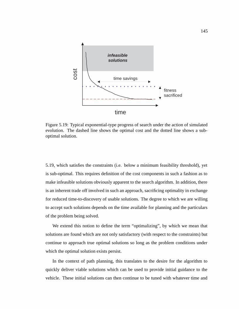
145

time

cost

infeasiblesolutions

time savings

fitnesssacrificed

Figure 5.19: Typical exponential-type progress of search under the action of simulatedevolution. The dashed line shows the optimal cost and the dotted line shows a sub-optimal solution.

5.19, which satisfies the constraints (i.e. below a minimum feasibility threshold), yet

is sub-optimal. This requires definition of the cost components in such a fashion as to

make infeasible solutions obviously apparent to the search algorithm. In addition, there

is an inherent trade off involved in such an approach, sacrificing optimality in exchange

for reduced time-to-discovery of usable solutions. The degree to which we are willing

to accept such solutions depends on the time available for planning and the particulars

of the problem being solved.

We extend this notion to define the term “optimalizing”, by which we mean that

solutions are found which are not only satisfactory (with respect to the constraints) but

continue to approach true optimal solutions so long as the problem conditions under

which the optimal solution exists persist.

In the context of path planning, this translates to the desire for the algorithm to

quickly deliver viable solutions which can be used to provide initial guidance to the

vehicle. These initial solutions can then continue to be tuned with whatever time and

146

processing capability is available to continue to push the corresponding cost closer to

the optimal value.

5.7 Multi-Objective Cost Evaluation

Inevitably, search over the space of paths to discover near-optimal, or optimalizing

routings involves tradeoffs between the various cost components. These tradeoffs illus-

trate the high sensitivity of EA performance to the relative value of the scalar payoff

function weights. This was evident in the examples described in which “component

conflicts” occur when one cost value increases while another is decreasing - leading to

a deadlock situation. Even with the simple scalar weighted penalty formulation used

throughout this chapter, there are situations where the effective “gains” corresponding

to each penalty term need to be changed to achieve the system goals. This corresponds

to modifications in the overall priority of the various objectives and suggests an adaptive

scheme employing a progress monitor. This monitor could assess the convergence rate

of the optimization and, in the case where a minimum is reached which fails to satisfy

the mission objectives, could affect changes to the penalty gains to allow behavior-

specific mutations to search for alternative solutions.

Given the variety of different forces influencing the search for paths (e.g. collision

avoidance, goal attraction, minimizing threat exposure, maximizing data value, min-

imizing fuel, time-of-arrival constraints, etc.), it seems that one might benefit from a

formulation which explicitly accounts for the existence of multiple objectives. In this

case, the cost components are not combined into a scalar value, but rather are kept as

components of a cost function vector, f(xj) ∈ RF , where F is the number of individual

cost functions.

The various tradeoffs involved between the different components of the cost can be

formalized by the notion of a Pareto optimal surface. This surface is defined such that

improvements along any given direction can only result at the expense of reduction in

value along at least one other direction. Essentially, one can think of multi-objective

147

evolutionary algorithms (MOEA) as a parallel search to discover this Pareto optimal

surface - or at least sample a sufficiently large number of points along it. Once this

surface is approximately known, one can choose the direction along which to move on

the basis of priority of the various objectives. For example, given the set of all paths

minimizing the distance to the goal, one can select from those along the Pareto surface

which have the highest probability of survival. The concept of Pareto-dominance is

illustrated in Figure 5.20(a)-(b).

f1(x)

f2(x)

1

1

2

3

1

Pareto optimaltradeoff surface

f1(x)

f2(x)

5

2

2

1

1

Pareto optimaltradeoff surface

(a) (b)

Figure 5.20: Illustration of the concept of Pareto dominance for (a) the minimization off1 and f2 and (b) the maximization of f1 and the minimization of f2.

The numbers near the points in the (f1, f2) space reflect the Pareto-rank of each of the

solutions. This rank value is equal to one plus the number of solutions which dominate

a given point. A vector, fa is said to dominate another vector, f b, denoted by fa ≺ f b,

if and only if f am ≤ f bm∀m ∈ 1, 2, . . . , F and faq < f bq for some q ∈ 1, 2, . . . , F.

Tan [99] develops a novel two-stage Pareto-ranking scheme that is capable of in-

cluding goals for each objective and the assignment of relative priorities. This scheme

has been embedded within a multi-objective evolutionary algorithm (MOEA) toolbox.

We applied this toolbox to the solution of the path planning problem presented in Sec-

148

tion 5.3.2. Recall that previously we had “filtered” the entire search space (found

through exhaustive enumeration) by layering successive requirements on the solution.

Now, we apply the MOEA toolbox to search this space based on a finite population con-

sisting of µ = 20 individuals. Rather than combining the cost components into a scalar

cost function, we instead treat the cost function explicitly as a vector of independent

factors, namely:

f j =

RangeGoal

1000ObstaclePenetrate

10(0.6− SurvivalProbability)

(5.21)

We present results obtained for two different prioritization schemes, summarized in

Table 5.1. The goal, or desired value for each cost component was set to zero. The

Table 5.1: Priority assignments for MOEA simulations.

priority

cost component Example 1 Example 2

RangeGoal 2 3

ObstaclePenetrate 1 1

SurvivalProbability 3 2

trajectories obtained for the Example 1 set of priorities is shown in Figure 5.21. One

first observes that the MOEA formulation is capable of finding trajectories which are

collision-free and reach the goal region. In fact, the trajectories discovered are essen-

tially the same as those which we discovered “by hand” in applying different conditions

to the entire search space. In this case, however, we were capable of identifying these

solutions with only a finite population and with no initial information with regard to

the location of the optimal solution. For the Example 1 priorities, the survival proba-

bility of the trajectories identified by the MOEA falls within a small range as noted in

149

the figure. We examine the effect of swapping the relative importance of RangeGoal

0 2 4 6 8 10 12−3

−2

−1

0

1

2

3

4

5

1

2

3

4

x position

y po

sitio

n

Ps range : [0.741, 0.742]

radarsites

goalregion

start

obstacles

after 100 generations with population size µ = 20

Figure 5.21: Trajectories obtained using Example 1 priority values after 100 MOEAgenerations.

and SurvivalProbability in Figure 5.22. Here, we find the corresponding change in

behavior to be consistent as, under the Example 2 priorities, the best solution found

has a higher survival probability than that found with the Example 1 priorities. Yet the

population as a whole exhibits greater variation in terms of survival probability. Finally,

one might wonder how the nature of the solution would change if SurvivalProbability

was given a priority of “don’t care”. The corresponding trajectories found using MOEA

under this case (with the priorities of the remaining objectives the same as Example 2)

are shown in Figure 5.23. Here one sees that the solutions still satisfy the collision-

free requirements and terminate at the goal. Their probability of survival, however, is

notable lower than that obtained in the previous cases.

Note, in presenting these MOEA results, we are not making the claim that a scalar

cost formulation could not discover similar trajectories. Rather, the main point is that

MOEA offers a desirable alternative to dealing with the sensitivity of the scalar cost

150

0 2 4 6 8 10 12−3

−2

−1

0

1

2

3

4

5

1

2

3

4

x position

y po

sitio

n

Ps = 0.77

Ps = 0.66

start

radarsites

obstacles

goalregion

Figure 5.22: Trajectories obtained using Example 2 priority values after 100 MOEAgenerations.

0 2 4 6 8 10 12−3

−2

−1

0

1

2

3

4

5

1

2

3

4

x position

y po

sitio

n

Ps = 0.77

Ps = 0.66

start

radarsites

obstacles

goalregion

Figure 5.23: Trajectories obtained when SurvivalProbability is given a “don’t care”priority with the remaining objectives keeping their Example 2 priorities.

151

formulation to the value of the weighting parameters.

5.8 Summary

This chapter has described the various cost components which are commonly used in

the context of path planning problems. In doing so, several issues with regard to the

non-uniqueness of the solution to most path planning problems were addressed, includ-

ing several strategies for avoiding local minima. It was shown that a combination of

fitness sharing and the addition of “repulsion” and “goal visibility” measures to the cost

function can reduce the tendency of the EA to get stuck in local minima over a class of

single-layer concave problems.

The notion of optimalization was introduced to formalize the fact that, in most cases,

it is more important to find “good enough” solutions as opposed to truly optimal solu-

tions. This is particularly the case when the planner must deliver updated trajectories to

the vehicle control system on a timely basis.

Finally, we briefly described the concept of a multi-objective evolutionary algorithm

which allows for the explicit assignment of priorities to the various components of cost.

In this fashion, the EA can make informed decisions as it chooses directions to move

along the approximate Pareto optimal surface as it is discovered.

152

Chapter 6

PATH PLANNING IN STATIC ENVIRONMENTS

In the previous chapter we detailed various issues related to the scoring of trial solu-

tions which are generated through the evolutionary process. In this chapter, we present a

series of simulation results which demonstrate the application of evolution-based tech-

niques to a number of different static path planning scenarios. As a means of assessing

the computational expense of evolution-based planning, we provide a numerical com-

parison against a graph search algorithm and another stochastic global optimization

algorithm when applied to this test suite of problems.

6.1 More than Shortest Paths

The typical path planning problem addressed in the literature is to find a “shortest” path

from a given initial state to some specified final state, where “shortest” refers to some

quantity such as distance, fuel, time, risk, or some combination thereof. Many of the

solutions obtained rely on some sort of graph/network representation of the problem

and find purely geometric solutions, often assuming some sort of nominal speed of the

vehicle between each node of the network (e.g. [55, 57]). When the mission objective

can be expressed in terms of an equivalent “shortest” path problem, these techniques

do indeed find optimal solutions. More general mission objectives, however, typically

require pairing the graph search with some sort of additional constraint and/or com-

binatorial optimizer (as done in [63]). For example, something as simple as requiring

the vehicle to arrive at a given location at a specified time (or, more generally within a

specified time window) requires a speed scheduler to try and find a way to manage the

vehicle speed along the shortest path such that it intersects the target point at the correct

153

time. Depending on the capabilities of the vehicle, such a solution may not exist, for

it may require the vehicle to stop or otherwise assume a speed outside of its “stable”

or usable range. An obvious example of this is an aircraft which will stall at a certain

minimum speed. Thus, shortest paths are not always the appropriate place to begin

searching for a solution to an arbitrary path planning problem.

Herein lies the strength of a population-based technique such as evolutionary pro-

gramming. Based on a “generate and test” paradigm, these approaches can generate

trial solutions whose dynamics are defined to be consistent with the maneuverability

constraints of the vehicle1. Further, the vehicle speed can be explicitly represented as a

tunable parameter of the population representation, eliminating the need for additional

speed scheduling in order to meet a time-of-arrival constraint. Because the individuals

in the population can represent complete paths, decisions regarding the fitness of indi-

viduals can be made based on much more complicated and general objective functions

than is possible with approaches which make decisions at each time instant. Essentially,

this allows a “delayed reward” feature in that intermediate decisions can be changed in

order to modify downstream performance. By allowing the point at which mutations

occur to vary over the length of an individual path, local modifications can be made to

compensate for sensed discrepancies or other unanticipated features of the environment.

Having discussed briefly the rationale for choosing evolution as an approach to path

planning, we now demonstrate its viability through a number of static environments.

We compare its performance relative to a graph search technique and an alternative

stochastic global optimization method.

6.2 Description of Numerical Experiments

In order to get a feel for the computational burden associated with evolution-based path

planning, we exercise it on a series of simple static test problems, which we will refer

1We will defer discussion of situations in which the maneuverability constraints are in error to Chapter7

154

to as P1 − P4 in the discussion that follows. It is noted that these simulations involve

navigation through “worlds” that are assumed to have unitless measures of distance.

These problems take place in static two-dimensional domains of size 50 units in each

direction. By static, it is implied that the location and size of obstacles present in the

environment is known and remains constant over the course of the search.

In each of the scenarios, the vehicle is initially located at the far left side of the

domain and the goal location is placed at the far right. The scenarios differ in the num-

ber and distribution of obstacles between the start and goal locations. These problems

were defined so as to represent problems of increasing difficulty for the evolution-based

planner in that they tend to increase the number of local basins of attraction which could

trap the planner prematurely prior to finding the goal location.

We will compare the performance of the EA planner against both a graph search

technique (A∗) and an approximation to uniform random search called Improved Hit

and Run (IHR) [100]. Each of the algorithms was coded as an m-file in MATLAB so

that reasonable comparisons could be made regarding relative computational expense,

counted in floating point operations (flops). Due to the fact that MATLAB effectively

does run-time compiling in terms of memory allocation, etc. the times reported in the

following sections should not be taken as representative of real-time performance which

would be exhibited if the various algorithms were coded in a compiled language such

as C or C++.

Graph Search Problem Statement

In the case of the graph search algorithm (A∗), the vehicle is constrained to move be-

tween the vertices of a graph, denoted by G(V,E), consisting of a set of vertices, V ,

and edges, E. The vertices represent the possible states of the vehicle, and the edges

represent the paths for transitioning between any two states on the graph. For the pur-

poses of these experiments, the domain was discretized at various resolutions in each

component direction (e.g. Nx, Ny = 10, 20, 30, 40, or 50 grid points along each axis).

155

Thus, we model the graph G as the physical location of the vehicle - the nodes rep-

resenting possible locations and the edges representing the set of possible paths. This

implies that the vehicle heading along any path through the graph network is defined

by the physical arrangement of nodes. The vehicle is initially located at (0, Ny/2) and

the goal location is specified as (Nx, Ny/2). Obstacle locations and sizes are scaled

such that they cover the same relative proportion of the free space regardless of the grid

resolution.

The problem thus consists of finding the shortest collision-free path contained in the

graph which connect the start and the goal nodes. For these examples, we assume that

each grid point is connected to all eight of its possible neighbors. These connections

represent the possible pathways for transitioning the vehicle between adjacent nodes

of the graph. Associated with each edge in the graph is a value, c(i, j), which is the

cost of traversing from node i to node j along their connecting arc. For the purposes

of these experiments, we model these costs to be the physical distance, d(i, j), between

any two nodes. Obstacles are represented by adding a value of OBSTACLE (where

OBSTACLE d(i, j)) to each arc which penetrates an obstruction.

Note that the solution obtained via search over the graph is purely spatial - there is

no no speed or time considered.

Stochastic Search Problem Statement

The path planning problem, as formulated via the instruction list or maneuver sequence,

consists of finding sequences of “decisions” at instants of time tk, for k = 0, 1, . . . , ,

which meet the requirements of a given problem. In this case, we are searching for paths

which avoid all known obstacles in the environment and terminate within a unit radius

of the goal location.

The “space” in which we search consists of integers. The intervals for each de-

gree of freedom corresponding to the instruction list and maneuver sequence span from

[Imin, Imax] and [ηmin, ηmax], respectively. The values of Imin and ηmin are both zero,

156

corresponding to theNOOP instruction. Recall that theNOOP instruction is included

to allow variable length paths to be represented by fixed length input vectors. The re-

maining instruction indices are defined in Table 4.2. The maneuver set considered in

these problems is given by the first five rows of Table 4.3. For the maneuver sequence

representation, the application interval space for each maneuver primitive was taken to

consist of integers in the range [∆tmin∆tmax] = [0, 5]. These intervals define the search

space, P , for each formulation.

As in the graph search problem statement, we assume that the initial and goal loca-

tions of the vehicle as well as the position and extent of all obstacles in the environment

are known and remain fixed over the course of the search. For the purposes of these

example problems, the sample time for evaluation of input sequences is ∆tk = 1 for all

tk ∈ 0, 1, . . . , ∗. Recall that ∗ represents the number of non-zero or active values in

a given input vector. Changes in vehicle heading are limited to maximum vehicle turn

rate, ψmax = 30/sec, i.e.

ψ[tk+1] = ψ[tk]± ψmax∆tk (6.1)

The vehicle speed is constrained in a similar fashion, restricted at each sample instant

to take on an integer value in the range [1, 3] units per time step. In these numerical ex-

periments, changes in speed over a given interval are fixed at ∆u = 1, with the sign of

the modification determined by the instruction or maneuver index. These perturbation

limits essentially define the vehicle’s performance bounds, limiting the extent and rate

at which the vehicle can change speed and direction. In particular, since the minimum

vehicle speed is constrained to be greater than zero, the vehicle cannot stop for an arbi-

trarily long time and/or instantaneously change its orientation. Note that the maximum

number of instructions and maneuvers, , is fixed prior to the start of the optimization

process. For the simulations shown, we choose a maximum of = 40 parameters in

each case. This corresponds to a maximum of 40 instructions and a maximum of 20 ma-

neuvers (with 20 application intervals). Generally, is chosen to be sufficiently larger

157

than that required if the lowest velocity is selected over a characteristic length of the

problem space. This gives the optimization process room to use larger velocities and

minimize the number of active instructions or maneuvers, ∗, required to reach the goal

location.

For the stochastic algorithms, a scalar performance function in the form of 5.2 was

used with the cost components specified in Table 6.1.

Table 6.1: Description of cost components for IHR (and EA)

Cost Component Description Weight

J1 RangeGoal 1.0

J21

RangeStart100.0

J3 ObstaclePenetrate 1000.0

6.3 Description of Algorithms

This section briefly describes the operation of each of the algorithms represented in the

numerical study.

6.3.1 Graph Search Algorithm

The graph search algorithm used for these studies is A∗ [101], a best-first technique for

finding shortest paths through a network. We model the domain as a graph, G(V,E),

comprised of a set of vertices, V and edges, E. Briefly, A∗ works by searching in a

wave-like manner, starting from the initial location, spanning outwards, and terminating

once the GOAL node has been reached2. Decisions regarding which direction to move

from a given node are made on the basis of the function:

2Note: A∗ can be equivalently formulated as a wave searching backward in time from the GOAL,terminating upon reaching the START node

158

f [n] = g[n] + h[n] (6.2)

where g[n] is the accumulated cost of reaching node n from the start node and h[n]

represents a heuristic estimate of the cost of traversing from node n to the GOAL. The

detailed operation of theA∗ algorithm is presented in Appendix B. At each iteration, the

node with the lowest cost, f [n], is chosen as the next node to expand. In this manner,A∗

is guaranteed to find the lowest cost (e.g. “shortest” obstacle-free) path between the start

point and the GOAL. This guarantee is subject to certain admissability requirements

on the heuristic estimates, h[n] (See Appendix B for details). Due to the finite size of

the search graph, the worst-case run-time of the algorithm can be determined (as this

would entail looking at each node in the graph prior to looking at theGOAL). Note that

the implementation used in these experiments pre-computes the arc costs and heuristic

values for each node in the grid prior to carrying out the search. The time required for

this computation is thus added to that required for the actual search over the graph for

the purposes of comparison with the other algorithms.

6.3.2 Stochastic Global Optimization Algorithm

The global optimization algorithm utilized for these numerical studies is the Improved

Hit and Run algorithm [100]. This algorithm represents one of a number of implemen-

tations of pure adaptive search, which attempt to approximate a uniform distribution

of the sampled space. Theoretical performance analysis of this algorithm has shown

that it can accomplish this in O(n5/2) operations/time [100] on elliptical (convex) pro-

grams. Although the path planning problem considered in this numerical comparison

is not strictly convex, this order of computation is useful for establishing the maximum

number of iterations in which we might expect to find a solution.

IHR is presented here assuming maximization of the objective function, f . Mini-

mization is achieved by maximizing−f . Unlike EAs, which typically evolve an entire

population of solutions simultaneously at each generation, IHR propagates only a sin-

159

gle solution at each iteration. We will denote this individual using a notation similar

to that for the EA, namely P (n), where we have dropped all superscripts and instead

have added an iteration counter, n. For the path planning problems considered here,

we model this individual solution using both the (a) instruction and (b) the maneuver

sequence formulations.

The assumption for IHR is that each of the dimensions in the search space can

be discretized over a finite interval. We utilize deterministic speed/heading change

operators (see Section 4.5.2) to produce the paths corresponding to both instruction list

and maneuver sequence input vectors. Essentially, one can think of the action of IHR as

a kind of mutation mechanism, providing an alternative means of manipulating the input

vector of the individual to try and discover trajectories which meet the requirements of

the problem.

We now describe in some detail the action of the IHR algorithm. To begin, an initial

feasible point in this space, P (0) ∈ P is specified. The algorithm then proceeds through

the following steps:

1. Evaluate the objective function value at the point P (n). Denote this value by

f(P (n)). (initially, n = 0)

2. Choose a random unit direction on a hypersphere of dimension , described by d.

3. Move along the line d a random distance (staying within the feasible space, P)

from the point P (n) to the point Q(n)

4. Evaluate the objective function value at the point Q(n), generating f( Q(n))

5. Use simulated annealing to update the best achieved cost value according to the

equation, υ ∼ U [0, 1] < a( Q(n)), the acceptance value. Upon acceptance of

a point Q(n) which improves the function value (e.g. f( Q(n)) > f(P (n)), the

temperature, T , is updated according to a cooling schedule (see Appendix A).

160

6. If accepted, set P (n + 1) = Q(n), otherwise P (n + 1) = P (n). Let n = n + 1.

Goto Step 1 unless the maximum number of iterations has been exceeded.

The process of moving through the search space, described in Steps 2-3 above, is il-

lustrated graphically in Figure 6.1 which shows a two-dimensional problem space. The

initial point is noted, as is the direction line generated in Step 2. As shown, the random

distance computed in Step 3 initially places the next point outside of the feasible region.

Note that there are several options available to deal with such a situation. One option is

simply to discard any points which fall outside ofP and select a new random distance to

move along the line defined by the direction vector d ∈ R. An alternative approach is

to extend the boundaries of the space and use a “reflection” operator to reflect infeasible

points discovered through the move along the line d back into the feasible space. This

concept is illustrated in Figure 6.1. Note, in particular, that the reflected point is shifted

x1

x2

feasible region

extended feasible region

reflectedpoint

initial point

next point

direction lineL

Figure 6.1: Illustration of the Improving Hit-and-Run operation (with reflection) in twodimensions.

161

(either via a ceil or floor operation so as to align with the discretization of the space.

Other options for handling the reflection and discretization are described in [100].

6.3.3 Evolutionary Algorithm

The evolutionary algorithm used for these comparison studies consists of a population

of size µ = 20 parents. The maximum number of input parameters, , is selected to

match that used by IHR ( = 40). Again, this corresponds to a maximum of 40 decision

points for the instruction list representation and a maximum of 20 maneuvers (with 20

associated application intervals). The population representations used are identical to

those used by IHR: (a) the instruction list and (b) the maneuver sequence. In both cases,

changes in speed and heading triggered by values in the input string are deterministic.

Creation of offspring involves the GA-like operations of crossover and mutation (with

p = 0.1) as described in Section 3.4.1. Since we use an “integer” string as opposed

to a “bit” string representation, flipping of a bit corresponds to the replacement of an

instruction at a given string location with another selected uniformly at random from

the set of possible instructions. Finally, we use a cost function identical to that used by

IHR.

6.4 Presentation of Results

Each of the algorithms was run for 20 trials on each of the test problems. Since the

stochastic algorithms are utilizing a FindGoal class of search, they require the defi-

nition of a stopping criteria. In this case, we deem the search to be successful once a

path has been discovered whose last point is within a ball of unit radius from the goal

location. In trials where this condition is not met, the stochastic algorithms are termi-

nated once a maximum of 10000 function evaluations has been exceeded. This value is

based loosely on the expected order of computation required for IHR to find the global

optimum, given the number of degrees of freedom considered in this problem ( = 40).

Note that A∗ needs no such stopping criteria as its worst-case behavior is deterministic,

162

involving the expansion of each node in the graph G(V,E) until finding the GOAL

node. The results for each algorithm will be presented separately and then summarized

at the end of this chapter as a means of demonstrating relative performance.

The following values are recorded upon termination of each trial:

• Approximate number of floating point operations (flops)

• Elapsed computation time

• Number of function evaluations

• Relative percentage of “obstacle detection” flops to total flops

Results for the stochastic search algorithms (EA and IHR) on each of the test prob-

lems include the distribution of paths and the distribution of cost obtained over each

of the trials at each iteration of search. The paths illustrate the different routings dis-

covered at the termination of each of the 20 trials, with the best (shortest) and worst

(longest) noted in each case. The cost distribution over the set of trials is slightly more

complex. It is represented at each iteration by four values: the minimum, maximum,

mean, and median cost value at each iteration. The minimum cost trace is marked by

a line through open circles, while the maximum cost trace is always the upper-most

line in each figure. The mean trace in each case consists of closed diamonds, while the

median trace is represented by a solid (red) line. Note that the calculation of these val-

ues includes all 20 trials, including those which have already exceeded the convergence

threshold. For the purposes of computing the mean and median, trials which have al-

ready converged at a given iteration are assigned a cost value of zero. The minimum

and maximum values effectively denote the “envelope” or extremes of cost value at

each iteration, while the mean and median values are useful for determining the “aver-

age” performance. Note that once a single trial has converged, the minimum cost bound

remains at zero. This is due to the fact that we include all trials in the computation of

the average performance.

163

6.4.1 Graph Search Results

The paths obtained using A∗ for each of the problem instances are shown below in Fig-

ure 6.2 (square obstacles) and Figure 6.3 (circular obstacles), indicated by the trails of

dark circles connecting the start and goal nodes. The extent of obstacles is marked with

an ‘x’ through the corresponding vertices. Note that the path obtained in each test prob-

lem depends on the shape and spatial extent of the obstacles, as would be expected. In

particular, alleys between obstacles which exist in the circular representation disappear

when the obstacles are modeled as square, forcing the planner to find a solution around

the obstacle field. Given the discretization of the domain in each case, the paths indi-

cated represent the shortest distance paths connecting the start and goal vertices. This

is true, even in cases (such as Figure 6.3(b) or (d)) when the path appears to oscillate

slightly. This effect, termed digitization bias, is described in more detail in Appendix

B, and results from the fact that only a finite number of angles is representable on the

discrete grid. In this case, because of the 8-connected structure of the graph, the vehicle

heading deviations are limited to multiples of 45 degrees. For the remainder of this

discussion we will restrict our attention to the “circular” obstacle representation as this

is the model assumed in the problem setups of the other algorithms.

Note that the computation complexity and number of function evaluations for A∗ is

largely determined by the size of the grid and the relative proximity of theGOAL to the

initial vehicle location. This dependency is detailed in Appendix E. Generally, these

factors increase with the square of the number of grid points in each direction. The dis-

tribution of obstacles has relatively little effect on the overall cost of solution. It should

be noted that the “obstacle detection” used in the A∗ solution was done by simply iden-

tifying the grid points which lie within any of the defined obstacles and assigning the

OBSTACLE cost to the value of traversing to such a node. This is a simple computa-

tion which is a function only of the number of obstacles, not their distribution. In order

to make a “fair” comparison with the other algorithms, it is necessary to approximate

the cost (in flops) of computing the intersection of a single path segment (between two

164

0 5 10 15 20 25 30 35 40 45 500

5

10

15

20

25

30

35

40

45

50

start

goal

0 5 10 15 20 25 30 35 40 45 500

5

10

15

20

25

30

35

40

45

50

goalstart

obstacles

(a) (b)

0 5 10 15 20 25 30 35 40 45 500

5

10

15

20

25

30

35

40

45

50

goalstart

obstacles

0 5 10 15 20 25 30 35 40 45 500

5

10

15

20

25

30

35

40

45

50

goalstart

obstacles

(c) (d)

Figure 6.2: Shortest paths found using A∗ on a 50x50 grid world with square obstacleson problems P1(a) through P4(d)

165

0 5 10 15 20 25 30 35 40 45 500

5

10

15

20

25

30

35

40

45

50

start

goal

0 5 10 15 20 25 30 35 40 45 500

5

10

15

20

25

30

35

40

45

50

start

goal

obstacles

(a) (b)

0 5 10 15 20 25 30 35 40 45 500

5

10

15

20

25

30

35

40

45

50

goalstart

obstacles

0 5 10 15 20 25 30 35 40 45 500

5

10

15

20

25

30

35

40

45

50

goalstart

obstacles

(c) (d)

Figure 6.3: Shortest paths found using A∗ on a 50x50 grid world with “circular” obsta-cles on problems P1(a) through P4(d)

166

nodes in the search graph) and a set of NO obstacles. This is done using the rectint()

function in MATLAB, which computes the intersection area between two rectangles -

in a manner identical to that shown in Figure 5.3. Results obtained in estimating the

computational load required as a function of path length and number of obstacles are

summarized in Table 6.2.

Table 6.2: Variation in “obstacle detection” flops required as a function of the numberof obstacles

Number of Path Segments Number of Obstacles

1 2 3 . . . NO

1 35 38 48 38 + 10(NO − 2)

2 39 47 62 47 + 15(NO − 2)

3 49 61 80 61 + 19(NO − 2)...

N 49 + 11(N − 4)

Since A∗ involves checking only a single path segment at a time, we are only con-

cerned with the top row of Table 6.2. Multiplying the computational effort correspond-

ing to the number of obstacles present in a given problem by the number of function

evaluations (e.g. nodes expanded) gives a flop count which can be compared with that

obtained through the other algorithms.

6.4.2 Improved Hit-and-Run Results

Each experiment involved twenty independent trials of the IHR algorithm starting from

an identical initial “state”, P (0), whose length was fixed at = 40 as described previ-

ously. In the case of the instruction list formulation, each “decision” in time, I[tk], for

tk = 0, 1, . . . , N was initially set to zero (the NOOP instruction). Thus, the initial

motion plan in each trial corresponds to “doing nothing” or, equivalently, staying put

167

at the initial location. A similar initial state was defined for the maneuver formulation,

with the initial sequence of maneuvers consists of only a single “go straight” maneuver

of duration 2 seconds. Thus, the algorithm is given no initial bias toward any particular

solution.

For brevity, in this section we present only the distribution of the best paths and

a measure of the rate of convergence achieved over each of the twenty trials on the

test problems, P1 − P4. Other data describing the set of experiments in more detail

is contained in Appendix E in Figures E.4 - E.11 which highlight the variation in:

(a) the elapsed computation time, (b) the best RangeGoal achieved, (c) the number

of function evaluations, (d) the number of flops, (e) the shape of the path found, and

(f) the dynamics or rate of convergence of the best solution obtained over the set of

20 trials on each problem. These sample data are included in the appendix in lieu of

noting standard deviations in the tabulation of results which follow in this chapter. The

rationale for this presentation being that the number of trials and the variation in these

quantities observed over this set of trials was not felt to be adequately described by a

normal distribution. Thus, the reader is referred to these plots and the discussion in

Appendix E for further detail.

IHR - Instruction List Results

Figure 6.4(a)-(d) show the different paths found by IHR over the series of 20 trials on

each of the test problems P1 − P4, respectively. These paths were obtained using the

instruction list formulation based on deterministic speed/heading changes. The longest

(black) and shortest (red) paths found in each case are denoted by the thick lines in each

figure. Obviously, IHR is successful in discovering many different paths to the goal over

the course of the 20 trials. Note that the paths discovered generally are not the minimum

length paths, but rather exhibit considerable wandering. This behavior is acceptable in

this case since no explicit penalty was placed on PathLength or PathAngle.

In order to get a feel for the extent of computation to achieve the paths shown

168

−10 0 10 20 30 40 50 60−10

0

10

20

30

40

50

60

x position

y po

sitio

n

start goal

−10 0 10 20 30 40 50 60 70−10

0

10

20

30

40

50

60

x position

y po

sitio

n

start goal

obstacles

(a) (b)

−10 0 10 20 30 40 50 60 70−10

0

10

20

30

40

50

60

x position

y po

sitio

n

start

goalobstacles

−10 0 10 20 30 40 50 60−10

0

10

20

30

40

50

60

x position

y po

sitio

n

start

goalobstacles

(c) (d)

Figure 6.4: Distribution of the paths found over 20 independent trials using IHR as apath planner. Based on deterministic speed/heading formulation with = 40 maximumlength instruction lists.

169

in Figure 6.4, we examine the nature of the cost achieved by IHR at each iteration

over the series of trials. We do so by examining the minimum, maximum, mean, and

median values occurring at each iteration computed over all 20 trials. Each of these cost

“descriptors” is overlaid on top of one another in Figure 6.5. The bottom line in each

figure is the minimum value while the top trace corresponds to the maximum value.

Note that we present the results in terms of the log10 of both the generation and cost

achieved in order to allow both large and small cost values to be distinguished on the

same plot.

The main point to be drawn from this figure is that IHR does indeed generate so-

lutions which penetrate obstacles - i.e. infeasible solutions. This is evident from the

points which lie in the range of 105 and is particularly noticeable in Figure 6.5(c),

where several trials continue to generate infeasible solutions until the final iteration.

Note also that the points at which the lowest black line crosses the (dashed) conver-

gence threshold correspond to the generation at which one of the experimental trials

first discovers a collision-free path to the goal. This is one measure which can be used

to gauge the relative difficulty of the different test problems. Another measure consists

of the average performance over the set of trials, as indicated by the mean (blue) and

median (red) traces in each of the sub-figures. Based on the point of first crossing,

it appears as though problem P1 is the easiest (crossing around generation 50) while

problem P3 is the most difficult (not crossing until generation 1600 or so). In compar-

ing the average performance, we reach a similar conclusion, as the P3 traces cross the

convergence threshold at the latest generation relative to the other problems. In fact, it

appears as if the mean and median costs over the set of all trials on problem P3 never

reach zero - which implies that at least one trial failed to terminate prior to the end of

10000 iterations.

In order to gain further insight into the relative performance of IHR over this set

of problems, it is of interest to directly compare some average measure of performance

over the set of 20 trials. For this purpose, we overlay each of the median traces con-

170

0 0.5 1 1.5 2 2.5 3 3.5 4−1

0

1

2

3

4

5

6

log10

(number of function evaluations)

log 10

(cos

t des

ripto

rs)

convergence threshold

0 0.5 1 1.5 2 2.5 3 3.5 4−1

0

1

2

3

4

5

6

log10


log 10

(cos

t des

ripto

rs)


(a) (b)

0 0.5 1 1.5 2 2.5 3 3.5 4−1

0

1

2

3

4

5

6

log10


log 10

(cos

t des

ripto

rs)


0 0.5 1 1.5 2 2.5 3 3.5 4−1

0

1

2

3

4

5

6

log10


log 10

(cos

t des

ripto

rs)


(c) (d)

Figure 6.5: Variation of best cost attained by IHR as a function of iterations for prob-lems P1 − P4 using the Instruction List input specification. Shown are the max, min(open circles), mean (closed diamonds), and median (red solid line) values over 20 trialsas a function of iteration.

171

tained in the sub-plots of Figure 6.5 on a single set of axes. Seen in this form, the

relative difficulty of the different test problems is immediately apparent, at least in

terms of the median cost. Here, we see that P1 is clearly the easiest of the problems

as would be anticipated given that there are no obstacles in the way. The differences

between the performance on the other 3 problems, however, are much more subtle,

particularly between P2 and P4. Nonetheless, this measure confirms our earlier specu-

lation that problem P3 was the most difficult for IHR to solve using the instruction list

formulation.

0 0.5 1 1.5 2 2.5 3 3.5 40

10

20

30

40

50

60

log10

(Number of Function Evaluations)

Med

ian

Val

ue o

f Cos

t

P1

P2

P3

P4

IHR Instruction List

Figure 6.6: Median cost over problems P1 − P4 for IHR instruction formulation.

IHR - Maneuver Sequence Results

Figures 6.7(a)-(d) show the different paths found by IHR over the series of 20 trials

on each of the test problems P1 − P4, respectively. These paths were obtained using

the maneuver sequence formulation based on deterministic speed/heading changes. The

longest (black) and shortest (red) paths found in each case are denoted by the thick lines

172

in each figure. As was the case in the instruction list results, IHR is successful in discov-

ering many different maneuver-based paths to the goal over the course of the trial set.

By comparison, however, the trajectories shown in Figure 6.7 exhibit much greater vari-

ation than those obtained using the instruction list input vector. This corresponds to the

fact that the maneuver-based formulation admits drastic changes in behavior based on

minor changes in the input vector. Again, these paths are by no means close to the “op-

timal” trajectories, for the most part, as no explicit penalty was placed on PathLength

or PathAngle. Such a penalty would have the effect of shortening the average length

of the path obtained and reducing their variation across different trials. Nonetheless, in

looking at the trajectories noted in red in Figures 6.7(b)-(d), one sees that at least one of

the paths obtained over the 20 trials on problems P2 − P4 is nearly optimal. Of course,

one also finds that the longest path (noted in black) is far from optimal, being rather

convoluted in nature.

Figure 6.8 shows the variation in the minimum, maximum, mean, and median cost

computed over the set of 20 trials on each of the four problem instances. Here, again, the

tendency of IHR to generate (and accept) solutions which penetrate obstacle constraints

is evident. Based on the points at which the minimum cost drops below the convergence

threshold in each sub-plot, it again appears that problem P3 was slightly more difficult

than the others when using IHR and the maneuver sequence input representation. Note,

however, that unlike in the instruction list case, the mean and median cost traces do in-

deed cross the convergence threshold prior to the termination of the maximum number

of iterations. This implies that, for the maneuver sequence, each of the 20 trials was

able to discover a collision-free trajectory satisfying the RangeGoal < 1 requirement.

Note also that the point at which the mean and median traces cross the convergence

threshold is nearly identical for problems P2 − P4. As a means of assessing the rela-

tive difficulty IHR experienced in solving the different test problems via the maneuver

formulation, consider Figure 6.9, which again overlays the median cost traces obtained

over each test problem. Based on this measure, one finds that again, problem P1 is by

173

−10 0 10 20 30 40 50 60 700

10

20

30

40

50

60

x position

y po

sitio

n

start

goal

−20 −10 0 10 20 30 40 50 60−20

−10

0

10

20

30

40

50

60

x positiony

posi

tion

start

goal

obstacles

(a) (b)

−20 −10 0 10 20 30 40 50 60 70−20

−10

0

10

20

30

40

50

60

70

x position

y po

sitio

n

start

goal

obstacles

−10 0 10 20 30 40 50 60−30

−20

−10

0

10

20

30

40

50

60

x position

y po

sitio

n

startgoal

obstacles

(c) (d)

Figure 6.7: Distribution of the paths found for problems P1(a)-P4(d) over 20 indepen-dent trials using IHR as a path planner. Based on maneuver formulation with = 20maximum maneuver segments.

174

0 0.5 1 1.5 2 2.5 3 3.5 4−1

0

1

2

3

4

5

6

log10


log 10

(cos

t des

ripto

rs)


0 0.5 1 1.5 2 2.5 3 3.5 4−1

0

1

2

3

4

5

6

log10


log 10

(cos

t des

ripto

rs)


(a) (b)

0 0.5 1 1.5 2 2.5 3 3.5 4−1

0

1

2

3

4

5

6

log10


log 10

(cos

t des

ripto

rs)


0 0.5 1 1.5 2 2.5 3 3.5 4−1

0

1

2

3

4

5

6

log10


log 10

(cos

t des

ripto

rs)


(c) (d)

Figure 6.8: Distribution of the maximum, minimum, mean, and median costs as a func-tion of iteration found over 20 independent trials using IHR as a path planner on prob-lems P1(a)-P4(d). Based on maneuver formulation with = 20 maximum maneuversegments.

175

far the easiest scenario. Further, one observes that the average (median) convergence

rate over the set of trials on problem P2 is significantly better in the region between

generations 10 and 300 or so. Despite this early advantage, however, the convergence

rate of P2 is seen to match that of problem P4 from approximately generation 300 and

onward. The corresponding trace for problem P3 is seen to lag behind just slightly,

again confirming that it was, on average, the most difficult of the problem scenarios.

One can also compare the relative difficulty of solving the various problem instances

0 0.5 1 1.5 2 2.5 3 3.5 40

10

20

30

40

50

60

log10


Med

ian

Val

ue o

f Cos

t

P2

P3

P4

P1

IHR Maneuver Sequence

Figure 6.9: Median cost over problems P1 − P4 for IHR maneuver formulation.

with the instruction list as opposed to the maneuver sequence formulation. Such a com-

parison is made in Figure 6.10, which gives the variation in the median cost over the set

of 20 trials as a function of iteration for each input specification. Note that the cost axis

in this figure consists of the actual value, not the log as in earlier plots. In each of these

figures, the solid line corresponds to the maneuver formulation while the dot-dashed

line represents the median cost using the instruction list. The relative performance of

the two techniques seems to depend on the nature of the obstacle distribution in each

176

problem. On problem P1, in which no obstacles are present, the performance of the two

input representations is nearly identical. Early on the instruction list shows better per-

formance, yielding to slightly better latter convergence of the maneuver sequence. In

comparing the instruction list trace across the various problems, one finds that it has a

tendency to initially “stick” at a poor value of cost (it even increase in (b)), and then ex-

hibit a series of relatively sharp jumps in improvement. This is in contrast to the nature

of the maneuver sequence performance which tends to be slightly more regular in its

average convergence rate. Based on these plots, one concludes that the IHR instruction

list formulation generally resulted in faster convergence early in the search. Over all

problems, however, the IHR maneuver sequence outperforms the IHR instruction list

in that the entire set of trials converges earlier (in terms of generation). We now turn to

see how EA performed over these same test scenarios.

6.4.3 Evolutionary Algorithm Results

Equivalent results to those presented for IHR in the previous section are depicted here

for the case of the evolutionary algorithm (EA).

EA - Instruction List Results

The variation in the types of paths found by EA using the instruction list input rep-

resentation is illustrated in Figure 6.11(a)-(d) for problems P1 − P4, respectively. As

compared with the IHR results in Figure 6.4, one sees that the spatial distribution of

paths using EA is considerably smaller. In particular, a majority of the paths discovered

over the set of trials tend to lie in the vicinity of the “shortest” path in Figures 6.11(b)-

(c), with a reasonably equal split around the obstacle pattern in Figure 6.11(d). As was

done in the IHR case, we illustrate the variation in the best cost function value present

in the population at each generation of the EA (Figure 6.12. A glaring difference as

compared with the results with IHR is that EA does not accept a single infeasible so-

lution which penetrates the obstacles. Thus, the maximum and minimum cost in each

177

0 0.5 1 1.5 2 2.5 3 3.5 40

5

10

15

20

25

30

35

40

45

50

log10


Med

ian

Val

ue o

f Cos

t

Problem P1

maneuver formulation discrete speed/heading

0 0.5 1 1.5 2 2.5 3 3.5 40

10

20

30

40

50

60

log10


Med

ian

Val

ue o

f Cos

t

Problem P2


(a) (b)

0 0.5 1 1.5 2 2.5 3 3.5 40

10

20

30

40

50

60

log10


Med

ian

Val

ue o

f Cos

t

Problem P3


0 0.5 1 1.5 2 2.5 3 3.5 40

5

10

15

20

25

30

35

40

45

50

log10


Med

ian

Val

ue o

f Cos

t

Problem P4


(c) (d)

Figure 6.10: Direct comparison of the median cost for both the Instruction List andManeuver formulations for problems P1 − P4 using IHR.

178

−10 0 10 20 30 40 50 60−10

0

10

20

30

40

50

60

x position

y po

sitio

n

goalstart

−10 0 10 20 30 40 50 60−10

0

10

20

30

40

50

60

x position

y po

sitio

n

goalstart

obstacles

(a) (b)

−10 0 10 20 30 40 50 60−10

0

10

20

30

40

50

60

x position

y po

sitio

n

goalstart

obstacles

−10 0 10 20 30 40 50 60−10

0

10

20

30

40

50

60

x position

y po

sitio

n

goalstart obstacles

(c) (d)

Figure 6.11: Distribution of the paths found over 20 independent trials using EA as apath planner on problems P1(a)-P4(d). Based on deterministic speed/heading formula-tion with = 40 maximum length instruction lists

179

figure provide relatively smooth bounds surrounding the distribution of costs over the

set of trials. Another key difference is that in none of the problem instances was the

maximum number of generations exceeded - the mean and median traces cross the con-

vergence threshold in each sub-plot. As before, it appears as if problem P3 was the

most difficult, requiring more generations on average before the convergence threshold

was exceeded. Note, however that this distinction is not as sharp as it was in the IHR

results. The relative difficulty of the four problems in the context of the EA instruction

list formulation is given in Figure 6.13, where the median cost traces have again been

overlaid on the same axes. Here, the relative difficulty of the four problems is readily

apparent. In fact, this plot verifies our initial design objective, which was to present four

problems of generally increasing difficulty to the EA planner. Note, however, that we

again obtain the result that P3 is slightly more difficult than the other test scenarios - as

indicated by the fact that its median trace is the last to reach the convergence threshold.

EA - Maneuver Sequence Results

In order to assess the relative performance of the maneuver sequence as compared with

the instruction list, we repeat the above experiments using EA to manipulate the maneu-

ver indices and application intervals for the same problems P1 − P4. The trajectories

discovered over each of the 20 trials on these problems is shown in Figure 6.14. As

compared with the corresponding plots in 6.7, one finds that the best (shortest) tra-

jectories discovered by the EA formulation are nearly optimal over all of the problem

instances. In particular, EA finds the straight path in problem P1 in 75% of the trials.

Again, the distribution of trajectories in path space is much smaller than that found

using IHR - the majority of the EA trajectories lie within a small neighborhood of the

optimal solution. We also illustrate the variation of cost descriptors for the maneuver

formulation, as illustrated in Figure 6.15. As compared with the EA instruction list

results, the traces in this figure exhibit much more drastic variation over the suite of test

180

0 0.5 1 1.5 2 2.5 3 3.5 4−0.5

0

0.5

1

1.5

2

log10


log 10

(cos

t des

ripto

rs)


0 0.5 1 1.5 2 2.5 3 3.5 4−0.5

0

0.5

1

1.5

2

log10


log 10

(cos

t des

ripto

rs)


(a) (b)

0 0.5 1 1.5 2 2.5 3 3.5 4−0.5

0

0.5

1

1.5

2

log10


log 10

(cos

t des

ripto

rs)


0 0.5 1 1.5 2 2.5 3 3.5 4−0.5

0

0.5

1

1.5

2

log10


log 10

(cos

t des

ripto

rs)


(c) (d)

Figure 6.12: Variation of best cost values (min, max, mean, and median) attained over20 independent trials by EA as a function of iterations for problems P1 − P4. Based oninstruction list formulation with = 40 maximum possible number of active instruc-tions.

181

1 1.5 2 2.5 3 3.5 40

5

10

15

20

25

30

35

40

45

50

log10


Med

ian

Val

ue o

f Cos

t

P3

P4

P2

P1

Instruction List

Figure 6.13: Median cost over problems P1 − P4 for EA instruction list formulationwith = 40 maximum number of instructions.

problems, particularly on problems P3 and P4. This corresponds to the difficulty posed

by these latter problems, as indicated by the fact that the crossing point at which the first

trial exceeds the minimum convergence threshold generally moves to the right as one

examines Figures 6.15(a)-(d). Focusing on the mean and median traces for these latter

problems, one sees that the initial rate of convergence is generally slower than that seen

in problems P1 and P2, although it exhibits the same general features stretched in time

(generation). We note in particular the difference in the mean and median cost traces in

problems P3 and P4. Notice that the median trace (shown in red) does indeed cross the

convergence threshold, while the crossing of the mean trace (blue dots) is either delayed

(Figure 6.15(c)) or does not occur at all (Figure 6.15(d)). This latter result implies that

at least one trial for the EA maneuver sequence did not converge on problem P4 prior

to the 10000 function evaluation limit.

The relative difficulty of the four problems in the context of the EA maneuver for-

mulation is given in Figure 6.16. Here, the relative difficulty of the four problems is

182

−10 0 10 20 30 40 50 60−10

0

10

20

30

40

50

60

x position

y po

sitio

n

goal

start

−10 0 10 20 30 40 50 60−10

0

10

20

30

40

50

60

x position

y po

sitio

n

goalstart

obstacles

(a) (b)

−10 0 10 20 30 40 50 60−10

0

10

20

30

40

50

60

x position

y po

sitio

n

goalstart

obstacles

−10 0 10 20 30 40 50 60−10

0

10

20

30

40

50

60

x position

y po

sitio

n

goalstart obstacles

(c) (d)

Figure 6.14: Distribution of the paths found over 20 independent trials using EA asa path planner. Based on maneuver formulation with = 20 maximum maneuversegments. Mutation only with pmaneuver = 0.1, ptime = 0.1.

183

0 0.5 1 1.5 2 2.5 3 3.5 4−0.5

0

0.5

1

1.5

2

log10


log 10

(cos

t des

ripto

rs)


0 0.5 1 1.5 2 2.5 3 3.5 4−0.5

0

0.5

1

1.5

2

log10


log 10

(cos

t des

ripto

rs)


(a) (b)

0 0.5 1 1.5 2 2.5 3 3.5 4−0.5

0

0.5

1

1.5

2

log10


log 10

(cos

t des

ripto

rs)


0 0.5 1 1.5 2 2.5 3 3.5 4−0.5

0

0.5

1

1.5

2

log10


log 10

(cos

t des

ripto

rs)


(c) (d)

Figure 6.15: Distribution of the maximum, minimum, mean, and median costs as afunction of iteration found over 20 independent trials using EA as a path planner. Basedon maneuver formulation with = 20 maximum maneuver segments. Mutation onlywith pmaneuver = 0.1, ptime = 0.1.

184

readily apparent. Note that the slope of the traces in this case, particularly for problems

P3 − P4, is much steeper than that obtained using the instruction list formulation. This

corresponds to the fact that the instruction list formulation tends to exhibit gradual, but

continual improvement in fitness. In contrast, the progress of the maneuver sequence

tends to be much more discontinuous in nature, marked by an initial period of sustained

stagnation punctuated by sudden improvement.

1 1.5 2 2.5 3 3.5 40

5

10

15

20

25

30

35

40

45

50

log10


Med

ian

Val

ue o

f Cos

t

P1

P2

P3

P4

maneuver sequence(mutation only)

Figure 6.16: Comparison of rate of convergence of median cost for problems P1 − P4

using the EA maneuver formulation. Mutation only with pmaneuver = 0.1, ptime = 0.1.

As a means of assessing the relative performance of the maneuver and instruction

list formulations, consider Figure 6.17, which shows the mean cost traces obtained over

each problem using both input representations. Note that we have included the results

obtained using crossover in addition to mutation for the maneuver sequence formula-

tion. For problem P1, we see that the maneuver sequence is slightly more effective, with

the effect of crossover being minimal. The performance of the different input represen-

tations on problem P2 is nearly indistinguishable. This is in contrast to problems P3 and

P4, where we find that the discrete instruction list formulation exhibits a notably faster

185

rate of convergence over the set of trials. Focusing on the instruction list trace in Figure

6.17(d), we see evidence of several of the trials stagnating near a cost value 35, corre-

sponding to the local minima trap present in the obstacle definition for P4. Despite this

stagnation, the rate of convergence of the instruction list formulation is matched only

by the mutation + crossover results in P4, where we have modified the mutation rates

to be pmaneuver = 0.4 and ptime, respectively. Note, however, that the mean value for

the instruction list trace goes to zero (indicating all trials having converged) faster for

both problems P3 and P4.

186

1 1.5 2 2.5 3 3.50

5

10

15

20

25

30

35

40

45

50

log10


Mea

n V

alue

of C

ost

instruction list maneuver (mutation only) maneuver (mutation + crossover)

Problem P1

1 1.5 2 2.5 3 3.50

5

10

15

20

25

30

35

40

45

50

log10


Mea

n V

alue

of C

ost


Problem P2

(a) (b)

1 1.5 2 2.5 3 3.5 40

5

10

15

20

25

30

35

40

45

50

log10


Mea

n V

alue

of C

ost


Problem P3

1 1.5 2 2.5 3 3.5 40

5

10

15

20

25

30

35

40

45

50

log10


Mea

n V

alue

of C

ost

instruction list maneuver11 (mutate only) maneuver11 (mutate + crossover)maneuver42 (mutate+cross)

Problem P4

(c) (d)

Figure 6.17: Direct comparison of the mean cost for both the Instruction List and Ma-neuver formulations (with and without crossover) for problems P1 − P4 using EA.Included in (d) is the effect of different mutation rates on problem P4.

187

6.4.4 Relative Performance Comparison

In this section we summarize the results of the numerical experiments carried out in

tabular form. For the stochastic algorithms (IHR and EA), we present the maximum,

minimum, and average values for each metric obtained over the series of trials on each

problem. SinceA∗ is a deterministic algorithm, we report only the mean values obtained

on each problem on a 50 × 50 grid. This averaging is done to wash out the minor

variations in computation time observed - it has no effect on the number of flops or

nodes expanded as this is determined solely by the algorithm and problem definition.

The reader is referred to Appendix E to get a better feel for the actual variation in

the different metrics over the set of trials. As mentioned previously, we do not give a

standard deviation value since the data collected are not well represented by a normal

distribution. This is due to the fact that often times the stochastic algorithms would

run to the maximum allotted number of function evaluations in situations where the

termination criteria was not reached. As such, the data often consists of several “bands”

of points - distinguishing between the subset of trials in which the algorithm was able

to reach the termination criterion and those in which it could not. A more detailed

comparison would thus consist of comparing the algorithms only over this successful set

of trial. For the purposes here, however, we did not wish to throw out the cases in which

the algorithm failed to find a solution in the number of allotted function evaluations.

Instruction List Formulation

Tables 6.3-6.6 describe the performance of the various algorithms on the four test prob-

lems, P1−P4. This data corresponds to the instruction list formulation for the stochastic

search algorithms (EA and IHR).

188

Table 6.3: Summary of results for problem P1 where = 40 for EA and IHR - usinginstruction list representation.

A∗ IHR EA

mean min max mean min max mean

Num. Evals 245 71 6707 2582 240 2560 835

Comput. Effort (Mflops) 0.024 0.12 12.6 5.05 .068 1.05 0.32

Elapsed Time (secs) 0.68 1.35 159.41 63.59 2.03 26.94 8.40

Table 6.4: Summary of results for problem P2 for = 40 for EA and IHR - usinginstruction list representation.

A∗ IHR EA


Num. Evals 1470 299 10000 4807 520 2300 1242

Comput. Effort (Flops) .041 0.59 21.11 9.95 0.31 1.95 0.99


Table 6.5: Summary of results for problem P3 with = 40 instructions for IHR and EA- using instruction list representation.

A∗ IHR EA


Num. Evals 2257 1642 10000 7850 960 4920 2681

Comput. Effort (Mflops) .051 3.33 21.83 16.53 0.86 5.55 2.83


189

Table 6.6: Summary of results for problem P4 with = 40 instructions for EA and IHR- using instruction list representation.

A∗ IHR EA


Num. Evals 2453 514 10000 5672 1020 2460 1696

Comput. Effort (Mflops) 0.054 1.09 21.92 12.02 0.99 2.86 1.78


Maneuver Sequence Results

In this section, we summarize the performance of the various algorithms on the four

test problems P1 − P4 when the input representation for the stochastic algorithms is

formulated as a maneuver sequence. The results for A∗ are simply copied from those

obtained in the previous section for purposes of comparison.

Table 6.7: Summary of results for problem P1 where = 40 for EA and IHR - us-ing maneuver sequence representation. Note: Mutation operator for EA consists ofmutation only with pmode = ptime = 0.1.

A∗ IHR EA


Num. Evals 245 22 5574 1297 140 460 243

Comput. Effort (Mflops) 0.024 .087 26.29 5.16 0.10 0.49 0.23

Elapsed Time (secs) 0.68 .571 173.72 34.44 1.29 5.94 2.76

190


A∗ IHR EA


Num. Evals 1470 338 10000 3181 360 1160 769

Comput. Effort (Mflops) 0.041 1.33 37.56 12.46 0.50 2.42 1.38



A∗ IHR EA


Num. Evals 2257 689 10000 4304 920 9980 3254

Comp. Effort (Mflops) 0.051 2.74 43.48 16.09 1.69 27.56 6.47



A∗ IHR EA


Num. Evals 2453 322 7350 2407 1880 9980 4086

Comp. Effort (Mflops) 0.054 0.77 32.98 9.88 2.62 19.41 6.60


191

Table 6.11: Comparison of results for problem P1 where = 40 for EA using maneuversequence representation to examine the effect of crossover on average performance.Note: mutation probabilities set to pmaneuver = ptime = 0.1.

EA mean values

(mutation only) (mutation + crossover)

Num. Evals 243 256

Comput. Effort (Mflops) 0.23 0.28

Elapsed Time (secs) 2.76 3.36

Table 6.12: Comparison of results for problem P2 where = 40 for EA using maneuversequence representation to see the effect of crossover. Note: mutation probabilities setto pmaneuver = ptime = 0.1.

EA mean values


Num. Evals 769 1066



Table 6.13: Comparison of results for problem P3 where = 40 for EA using maneuversequence representation to see the effect of crossover. Note: mutation probabilities setto pmaneuver = ptime = 0.1.

EA mean values


Num. Evals 3254 2488



192

Table 6.14: Comparison of results for problem P4 where = 40 for EA using maneuversequence representation to see the effect of crossover. Note: mutation probabilities tovalues indicated.

EA mean values

mutate only mutation + crossover

pman=0.1ptime=0.1

pman=0.4ptime=0.2

pman=0.1ptime=0.1

pman=0.4ptime=0.2

Num. Evals 4086 3544 2587 4411

Comput. Effort (Mflops) 6.60 12.07 4.98 16.24

Elapsed Time (secs) 97.11 107.89 66.93 143.62

6.5 Summary of Findings

We first make several general comment regarding the relative difficulty of the four test

problems observed through these experiments. Recall that we originally intended for

the four problems to increase in difficulty - with problem P4 posing the most challenge

due to the presence of an obvious potential minima trap. Based on the experimental re-

sults, however, we found that this was generally not the case. Instead, problem P3 was

seen to cause the algorithms the most fits. This result can be rationalized, however, by

considering the nature of the paths which the algorithms tended to discover. Because of

the inclusion of the repulsion term (inversely proportional to RangeStart) in the cost

function, the local minima trap was generally avoided, causing partial paths to naturally

end up to the “outside” of the obstacles in problem P4. At this point, with the goal es-

sentially in clear view, it was a relatively easy task to connect the free ends of these paths

to the goal location. On the other hand, problem P3 has a considerably smaller propor-

tion of “goal visibility” as compared with the other test scenarios. Also, the spacing of

the obstacles and the gaps in between them are such that small changes are typically

necessary for a trajectory to squeeze through. This explains why the instruction list for-

mulation outperformed the maneuver sequence, as changes in an instruction have very

localized effects in terms of the shape of the trajectory. By comparison, changes in a

193

maneuver index can cause much more dramatic changes in the trajectory. In fact, this

relative degree of motion through the space exhibited by the maneuver sequence and

instruction list formulations suggests a hybrid scheme in which the population initially

consists of a maneuver sequence and then transitions to an instruction list representation

for the purposes of fine-tuning the trajectory.

In assessing the performance of the various algorithms, we take the deterministic

results of A∗ as a baseline and comment on the mean values obtained with IHR and EA

using both the instruction list (Tables 6.3 - 6.6) and the maneuver seqeuence (Tables 6.7

- 6.10) input definitions. On the simplest problem, P1, in which there are no obstacles

present, A∗ is seen to have a clear advantage in terms of average performance across

all metrics. As might be expected, however, due to the stochastic nature of the IHR and

EA algorithms there are instances when the lowest values obtained on a given trial are

competitive with those of A∗. Again, however, this “luck of the draw” cannot be relied

on in general - it is the average performance of the stochastic algorithms over a number

of trials which is important.

As one moves through the different problem instances, several trends appear:

• EA generally outperforms IHR over all metrics as the problem complexity in-

creases. This holds for both the instruction list and maneuver sequence input

definitions.

• The elapsed computation time for A∗ catches up and even exceeds that required

by EA (mean value - using the instruction list input definition).

This first trend is not too unexpected in that the purpose of a global optimization

algorithm such as IHR is not necessarily to find an answer fast - but simply to find the

global optimum through an increasing uniform sampling of the search space over time.

This implies that IHR is less likely to be stuck in local minima traps as compared with

EA whose sampling is biased by the forces of natural selection.

194

Admittedly, the second trend listed above is due in large part to the run-time compil-

ing of MATLAB and its associated inefficiency in executing for loops. Given that the

evolutionary process is a “generate and test” procedure involving excessive for loops

as well (not to mention the generation and evaluation of paths), this disadvantage is

shared by all the algorithms presented. A caveat in generalizing this result, however, is

that the number of floating point operations for A∗ does not grow in a similar fashion.

The performance of these algorithms in C/C++ can not necessarily be inferred by these

results. Nonetheless, given the use of A∗ in real-world applications in the literature (see

Chapter 2), these results are encouraging in that EA might be at least viable for the

purpose of path planning in near real-time. Note that this second trend does not hold in

the maneuver sequence formulation, where the mean value of computation time for EA

is seen to be greater than two times that of A∗ on the most difficult problem instances

(P3 − P4).

In examining the effects of crossover on the performance of the EA maneuver se-

quence in solving problems P1 − P4 (Tables 6.11 - 6.14), we note an interesting trend.

Initially, we hold the mutation probabilities on the application time and maneuver se-

lection at the values ptime = pmaneuver = 0.1. On the “easier” problems (P1 − P2),

crossover evidently slightly degrades the average convergence time. On the other hand,

crossover is seen to provide a significant improvement in terms of reducing the conver-

gence time on the more “difficult” problems (P3−P4) - even though the computational

effort involved in implementing crossover actually increases. From this result, one can

infer that the relative benefit of crossover is tied to the twists and turns required of the

solution trajectory. In loosely constrained environments, the added computational com-

plexity and increased variation in trajectories provides no appreciable value. On the

other hand, as the percentage of free space becomes smaller, the additional “curiosity”

caused by crossover of individuals provides an advantage over mutation alone. Note,

however, that despite this improvement in average convergence time, the performance

of the (mutation + crossover) maneuver sequence still does not match that obtained

195

using the instruction list formulation.

Also included in Table 6.14 are the average measures obtained for the case when

the mutation probabilities for time and maneuver were increased to ptime = 0.2 and

pmaneuver = 0.4, respectively. Here we see that the increased mutation rate has a no-

ticeable negative impact on performance when measured in terms of the average “time

to convergence”. This tendency is confirmed in looking closely at the corresponding

trace in Figure 6.17(d), which, although having a reasonable good initial rate of con-

vergence, exhibits considerable flattening over the latter iterations. We highlight the

effect of increased mutation probability in Figures 6.18 - 6.19 both with and without

crossover, respectively. Here we see that the effect of crossover is to increase the early

rate of convergence while slowing the later fine tuning of the trajectory in the vicinity

of the optimal solution. This is indicated by the crossing of the two traces in these

figures. Indeed, the mean value for mutation only goes to zero faster than that when

crossover is included in the generation of offspring. This is consistent with the fact that

“smaller” mutations are desired once the search has focused near an optimal solution.

Such a result suggests an adaptive offspring production mechanism which utilizes large

rates when the solution is “far” from optimal and then gradually reduces the mutation

probabilities as the optimal solution is approached.

Note that the static environments considered in this chapter represent the bare min-

imum in terms of capabilities required by a path planning algorithm for an autonomous

vehicle. We have not included any additional targets for the vehicle to observe, nor

have we modeled any time-of-arrival constraints. In fact, implementation of A∗ in such

situations, although possible, leads to a dramatic increase in computational effort - a

problem which is only amplified as one begins considering coordinated planning for

multiple vehicles. In this case, one needs to introduce a separate combinatorial op-

timizer (similar to [64]). It may not even be feasible to cast realistic path planning

problems in a framework consistent with a graph search formulation. In such situa-

tions, stochastic algorithms such as EA have a distinct advantage in that, as long as the

196

1 1.5 2 2.5 3 3.5 40

5

10

15

20

25

30

35

40

45

50

log10


Mea

n V

alue

of C

ost

Problem P4

(mutation only)

ptime

= 0.2p

man = 0.4

ptime

= 0.1p

man = 0.1

Figure 6.18: Comparison of different mutation rates on mean cost value vs. generationfor problem P4 using mutation only to generate offspring.

1 1.5 2 2.5 3 3.5 40

5

10

15

20

25

30

35

40

45

50

log10


Mea

n V

alue

of C

ost

3.6 3.8 40

0.5

1

1.5

2

log10


Mea

n V

alue

of C

ost

Problem P4

(mutation + crossover)

ptime

= 0.2p

man = 0.4

ptime

= 0.1p

man = 0.1

Figure 6.19: Comparison of different mutation rates on mean cost value vs. generationfor problem P4 including crossover in generating offspring.

197

problem can be modeled via population and expressed in terms of some sort of (vector)

cost function, solutions can be evolved. Thus, although EA is not the path planner of

choice in every situation, it holds significant potential for solving an array of problems

which are out of reach of other path planning techniques.

198

Chapter 7

PATH PLANNING IN DYNAMIC ENVIRONMENTS

In this chapter, we extend earlier results by treating dynamic scenarios involving

“annoying” environments. These environments range from the sudden appearance of

“pop-up” obstacles to the tracking a non-stationary target through a moving obstacle

field. By treating such scenarios, we illustrate the ease with which complex problems

can be handled by EA through minor changes in the definition of the environment (e.g.

the cost function) used to shape solutions. What distinguishes this class of problems

from the static problems treated in the previous chapter is the need for the evolutionary

algorithm to search through both space and time simultaneously. We refer to these

environments as annoying rather than adversarial because we assume that the obstacles

and targets follow pre-determined trajectories which do not change in reaction to the

vehicle’s motion. Instead, their motion is intended only to disturb the planner, making

its task more complicated.

7.1 Overview

Inevitably, planning involves searching forward in time, approximating the future inter-

action of the vehicle with the environment and the effects of its actions. In a static, pas-

sive environment, this involves construction of spatial trajectories which are collision-

free and satisfy the mission objectives. Time enters explicitly only in situations in-

volving time-of-arrival constraints, or threats whose potential lethality changes in time

or with duration/proximity of exposure. When a vehicle must dodge moving obsta-

cles to intercept moving targets, however, the space which must be searched inherently

includes both spatial and temporal dimensions. Not only must the vehicle’s state be

199

propagated forward in time, but so must that of the targets and threats. Either exact

knowledge or an estimate of the target and threat motion must be utilized in order to

maximize the probability that the vehicle can reach the target(s) while simultaneously

avoiding the moving obstacles. This problem is further complicated when the vehi-

cle must navigate through regions of the environment where the effective “terrain” can

change over time. For example, assuming that passage through a particular region gives

the vehicle a tactical or otherwise advantage, it might behoove the vehicle to “stall”,

waiting for strong headwinds to subside rather than taking an alternative route.

For simplicity, we limit our focus to robotic vehicles which can be modeled as a

single rigid body, parameterized by a characteristic length. For purposes of collision

detection, we model the vehicle as a circle (2D) or sphere (3D) with a fixed radius. In

general, motion planning for an articulated body connected by various joints could be

handled through straightforward extension of the discussion presented here.

It is reiterated that the approach taken in this thesis is that we do not seek to find

a unique, globally optimal solution to each planning problem. Due to the dynamic

nature of the various entities involved (environment, mission, vehicle), as well as the

need for time-constrained delivery of trajectories in near real-time, we instead search

for solutions which are “good enough”. We thus adopt an algorithmic approach which

continually probes the environment, repeatedly solving a series of different planning

problems in rapid succession. We argue that the notion of a problem yielding a single

optimal solution is meaningless in the presence of uncertainty - any supposedly “opti-

mal” path is likely to become obsolete at a moment’s notice.

7.2 Planning Amidst a Changing (but Non-Moving) Environment

In this example we use the baseline continuous speed/heading formulation (see Sec-

tion 4.5) applied to a single vehicle routing problem through a changing obstacle field.

Under this framework, we treat the vehicle speed as a discrete integer in the range

u[k] ∈ 1, 2, 3 and the vehicle heading as a continuous real-valued number in the

200

range ψ[k] ∈ [0, 2π]. Changes in heading and speed are triggered based on values in the

instruction list and implemented using the stochastic perturbations (see Section 4.5.1),

in which perturbations are limited to ∆umax = ±1 and ∆ψmax = ±30 over any given

interval.

A scalar cost function is used in this simulation, containing the cost components:

f(xj) = RangeGoal(xj)

+ 1000ObstaclePenetrate(xj)

(7.1)

The size of the population is taken to consist of µ = 20 individuals, where the length of

each individual is allowed to vary from zero to a maximum of 100 instructions. Gen-

eration of offspring consists of randomly modifying a maximum of 5 instructions per

parent, as well as adding or deleting an instruction from the end of each parent’s list as

described in Section 4.5.1. Note that every 10 generations, we replace the 5 worst per-

forming individuals in the population with 5 new parents, initialized at random. This is

done so as to provide the EA with the opportunity to utilize these new individuals which

have yet to be biased by previous experience in the environment. The tournament se-

lection used in this and all other simulated results reported consists of the q-fold binary

tournament as described in Section 3.4.3. Here, we define the number of competitions

in each tournament to be equal to µ/2 = 10.

We show the results of a typical simulation under these conditions in terms of sev-

eral “snapshots” taken over the course of the experimental run, presented in Figure 7.1.

Note that these results were obtained through an interactive simulation in which the

obstacles were placed “dynamically” by the author while the simulation is taking place.

The snapshots below capture the state of the evolution at a number of such points. In

each sub-figure, the solid line corresponds to the best available solution at a given gen-

eration whereas the dashed lines show a portion of the remaining population. This latter

group of individuals is included in order to illustrate the distribution of the population

relative to the best available solution and how this distribution changes over time.

In Figure 7.1(a), we see that the population has branched out into three viable

201

routes through the obstacle field, with the most direct route currently providing the

most promising solution (as indicated by the solid line). Upon the detection of an unan-

ticipated obstacle (labeled as 12) blocking this path (Figure 7.1(b)), the population is

seen to evolve to abandon the direct route and occupy the two alternatives around the

left side of the obstacle field. In Figure 7.1(c), the vehicle is given “intelligence” in-

formation regarding the location of an observation target at point A. Here we see the

population again adjust to isolate two primary routes, with the faster route around the

outside of the field identified as the preferred path. Figure 7.1(d) shows the converged

state of the population as the path satisfies the mission objectives, having reached the

target and terminated successfully at the GOAL.

In Figure 7.2, we present an additional 2D scenario which can be interpreted either

in terms of a ground vehicle trying to reach a goal on the other side of a bridge, or

alternatively, in terms of an air vehicle attempting to fly between a set of buildings. We

will adopt the former interpretation for the purposes of discussion. Here, the vehicle,

originating at point S, must cross one of two possible bridges to reach the GOAL on the

other side of a ravine or river (represented by the rectangular obstacles). Note that a

separate boundary has been created along the top and sides of the environment in order

to force the search to concentrate on using the bridges to cross the river. Without this

boundary, the planner tended to find paths around the “outside” of the water (i.e. outside

of the figure). The planner is given no prior knowledge that biases its trajectories toward

the exact locations of the bridges. It discovers the bridges solely on the basis of creation

of trial solutions which cross to the other side.

The conditions for this simulation are identical to those described in the previous

example, with the exception that in this case, we do not inject random individuals into

the population. Figure 7.2(a)-(b) show the initial distribution of paths and the state

of the search after approximately 30 generations, respectively. Here we see that the

planner successfully uses the left-most bridge to reach the GOAL. At this point, a set

of additional obstacles are inserted (interactively while the search is running) as shown

202

−20 −15 −10 −5 0 5 10 15 20−20

−15

−10

−5

0

5

10

15

20

1

2

3 4

5

6

7

8

9

10

11

SC

GOAL

−20 −15 −10 −5 0 5 10 15 20−20

−15

−10

−5

0

5

10

15

20

1

2

3 4

5

6

7

8

9

10

11

12

SC

GOAL

(a) (b)

−20 −15 −10 −5 0 5 10 15 20−20

−15

−10

−5

0

5

10

15

20

1

2

3 4

5

6

7

8

9

10

11

12

SC

GOAL

1

−20 −15 −10 −5 0 5 10 15 20−25

−20

−15

−10

−5

0

5

10

15

20

1

2

3 4

5

67

8

9

10

11

12

SC

GOAL

1

(c) (d)

Figure 7.1: Dynamic planning example through a changing obstacle field. Frames (a)-(d) show snapshots at various generations while evolution reacts to user modificationsto the environment

203

in Figure 7.2(c), triggering the movement of the population away from the left bridge

and towards the right-most crossing. By generation 100, the population has found a

way to squeeze through the opening and has reached the GOAL, as indicated in Figure

7.2(d).

−20 −15 −10 −5 0 5 10 15 20−20

−15

−10

−5

0

5

10

15

20

1

2

3

4

5

6

7

SC

GOAL

−20 −15 −10 −5 0 5 10 15 20−20

−15

−10

−5

0

5

10

15

20

1

2

3

4

5

6

7

SC

GOAL

(a) (b)

−20 −15 −10 −5 0 5 10 15 20−20

−15

−10

−5

0

5

10

15

20

1

2

3

4

5

6

7

8

9

SC

GOAL

−20 −15 −10 −5 0 5 10 15 20−20

−15

−10

−5

0

5

10

15

20

1

2

3

4

5

6

7

8

9

SC

GOAL

(c) (d)

Figure 7.2: Ground vehicle planning - frames (a)-(d) show the reaction to an unantici-pated blockage of the left-hand bridge after initial plan creation.

204

7.2.1 Handling Terrain Changes

In this section, we present a simple example which illustrates the ability of the EP-

based planner to search to find feasible, near-optimal paths through spatially varying

“terrain”. The environment in this example initially consists of a uniform windfield,

pointing to the north (upwards along the page), where the windspeed is defined to be

the maximum vehicle speed, i.e.‖w‖ = umax = 3. As shown in Figure 7.3, the vehicle

starts at location S and is tasked with finding a path to a target location, markedGOAL.

Fixed obstacles are represented by the numbered, open circles in the figure.

The effects of the wind are included in the evaluation of the physical trajectory by

modifying the effective speed of the vehicle over a given interval. First, the instruction

list for each trial solution is mapped into a corresponding sequence of speeds and head-

ings, as defined by the speed/heading change operators. In this case, we again use the

stochastic version of these operators. The values in this speed sequence are modified

to account for coupling with the environment by adding the average wind components

over each interval:

uxeff [tk] = u[tk]cos(ψ[tk]) + wx[tk]

uyeff [tk] = u[tk]sin(ψ[tk]) + wy[tk] (7.2)

Given this sequence of effective speeds (in terms of their inertial components), the

physical locations of the vehicle at each sampling instant are then obtained.

Running the EP-based planner through this initial scenario results in the left-most

(dashed) path shown in Figure 7.3. Note that the arrows emanating from each path rep-

resent the vehicle orientation at each time step. As expected, the trajectory “delivered”

once the planner finds a complete path (i.e. RangeGoal(xj) < Rε) essentially follows

the wind field, making slight diversions as necessary to route around the fixed obstacle

field.

To demonstrate the adaptation of the population, we assume that the vehicle be-

gins moving along this left-most path when it becomes aware (based on an assumed

205

−20 −15 −10 −5 0 5 10 15 20−20

−15

−10

−5

0

5

10

15

20

1

2

3

S

GOAL

Range to targets:Range to goal:Energy value:

0.539610

541

mode:

gen:0

53

C

path prior to inversion (generation 22)

path after detection(generation 53)

Figure 7.3: Planning through an “annoying” wind field. A localized inversion triggersa re-plan as indicated by the right-most path.

updated forecast or via on-board sensing) that the direction of the wind immediately in

front of it has changed direction, now pointing downwards. In re-evaluating the current

population in light of this “new” environment, the population performs quite poorly,

even heading backwards from its intended direction. This encourages the development

of “new” offspring with different “behavior” which better match this changed environ-

ment. The results of the re-planning are highlighted in the right-most path of Figure 7.3,

where we see that 30 generations after discovering the discrepancy in wind direction,

the planner has “corrected” the motion plan to go around the outside of the downward

pointing cells. This is the best course of action in the absence of any information or

estimate of the duration over which the wind inversion is expected to last. If such an es-

timate were available, it could be incorporated to allow alternative strategies including

a potential “stall” tactic waiting for the inversion to pass.

206

7.3 Dodging Moving Obstacles

We now turn to the problem of finding a target amidst a moving obstacle field - as might

be the case in an adversarial environment. For the results presented here, we assume

that the planner has perfect knowledge with regard to the motion of the obstacles in

time. In other words, the planner can always deduce the future “intent” of the obstacles

by accessing its position at any point in time. This is admittedly a major assumption, but

is used here to facilitate demonstration of the basic capability of the EP-based planner

to handle such scenarios. Implementation of this capability is possible by modifying

the obstacle penetration penalty to account for the motion of the obstacles in time to

check for possible future collisions. Here, we assume that the obstacles do not “react”

to the action of the vehicle.

For the purposes of this example, the initial position of each obstacle is assumed

known to the planner, and the obstacles are assumed to move along pre-defined straight-

line trajectories at a constant velocity. This allows the obstacle position at any future

time to be easily determined. Orienting the path-bounding rectangles along each path

segment facilitates rapid collision checking in the local frame of the path segment. This

technique is selected based on the assumption that the motion of the obstacles is in-

significant between sampling instants of the path motion - in other words, the obstacle

cannot suddenly jump from one side of a path segment to another between samples. If

this assumption is violated, an alternate scheme must be used. A better solution con-

sists of running a generalized collision detection calculation based on the rectangles

bounding the vehicle motion segment and obstacle motion between samples. This in-

creased complexity, however, is not necessary for the purposes of demonstrating the

basic concepts.

As an illustration of the capability of the EP planner to find routes through a dy-

namic obstacle field, consider the snapshots shown in Figures 7.4(a)-(c). These results

were obtained with a population size µ = 30, with all other parameters defining the

207

simulation identical to those of the previous examples. In addition, in this case, we

allow for the addition of multiple instructions (up to 10) to the end of each list. Obsta-

cles are represented as the shaded circles and the vehicle is represented by an open disk

with an arrow indicating its orientation and direction of travel. This example problem,

modeled after that presented in [45], involves planning through a set of obstacles which

are converging towards the vehicle. The direction of travel of each obstacle is defined

in multiples of 15 from [180 − 270]. The speeds of the obstacles in this case is set

to 1.25 units per timestep, chosen to be less than the maximum achievable speed of the

vehicle (umax = 3). Figure 7.4(a) shows the population once the planner has delivered

a complete motion plan (indicated by the thicker solid line in each sub-figure). Here

we have used a population size µ = 30. Note that several alternative routes around the

obstacle field are represented. Figures 7.4(b)-(c) show the vehicle executing a sharp

turning maneuver in order to clear the “wave” of obstacles, leaving a clear path to the

GOAL. Again, we do not claim this to be a unique solution, just a feasible one. Addi-

tion of secondary optimization criteria (minimum time, minimum fuel, etc.) might well

change the nature of the solution obtained.

7.4 Tracking a Moving Target Amidst Moving Obstacles

We now further complicate the planner’s task by allowing theGOAL location to change

with time. Thus, it must solve the problem of tracking a moving target while simulta-

neously avoiding moving obstacles. Again, we assume that the planner has perfect

knowledge regarding the GOAL position at any instant of time. The GOAL is given

a simple, straight line trajectory and its speed is limited to be less than the maximum

achievable speed of the vehicle. This allows the planner to catch the GOAL from be-

hind in addition to “intercepting” it in the traditional sense. In maneuvering around the

dynamic obstacles, the vehicle has two options. If it is faster than the obstacles, it can

navigate around them. If it is slower, it must wait for them to pass and then proceed

along its way. Note that we do not constrain the time of capture in this example, but

208

-30 -20 -10 0 10 20 30 40-30

-20

-10

0

10

20

30

40

S

2

3

4

6

7

timestep = 1

2

3

4

6

7

GOAL

x position

y po

sitio

n

(a)

-30 -20 -10 0 10 20 30-30

-20

-10

0

10

20

30

timestep = 12

2

3

4

6

7

GOAL

x position

y po

sitio

n

(b)

-30 -20 -10 0 10 20 30-30

-20

-10

0

10

20

30

timestep = 15

2

3

4

6

7 GOAL

x position

y po

sitio

n

(c)

Figure 7.4: Navigation through a converging obstacle field toward a fixed target. Frames(a)-(c) show snapshots in time during “execution” of the delivered trajectory.

209

rather, allow it to be a free parameter.

In this example, a moving “field” of five obstacles of various radii is set in motion

along vertical trajectories at different speeds - each of which is set to less than the

maximum vehicle speed. Obstacles 1, 3, and 5, are set in motion in the negative y-

direction with a speed of 1 unit per timestep. Obstacles 2 and 4 move upwards with

a speed of 1 unit per timestep. The radius of the vehicle disk in this case is set to 2

units. The vehicle is tasked with visiting a fixed target (denoted by the circle with a

red ‘X’) and then intercepting the moving GOAL. The “execution” of the delivered

plan is captured in Figures 7.5(a)-(c). The GOAL trajectory is indicated by the dashed

line in each figure. Here we see that the EP-based planner finds a route which allows

the vehicle to reach the target, squeezing between obstacles 3 and 4 and successfully

capturing the GOAL at timestep 30.

7.5 Adapting to Failures

To illustrate the ability of the evolution-based planner to adapt its plan based on vehicle

capabilities, consider the situation depicted below in Figure 7.6. Here, the vehicle is

tasked with navigating from its initial location (-10,-10) and orientation (−45) in order

to reach the goal location (25,25) by time tk = 35.

In this example, we define the population using the maneuver sequence formulation,

with the available maneuvers consisting of go straight, turn right, turn left, speed up

or slow down. We treat the application interval as a continuous variable in the range

0 ≤ ∆tk ≤ 5 and use a stochastic (Gaussian) perturbation to adjust these values over

the course of the search.

We utilize two different cost functions in this example. Prior to failure, we simply

specify path performance in terms of the distance from the end of a trial path to the

goal, evaluated at tk = 35:

J1 = RangeGoal(xj [tk = 35]) (7.3)

210

−40 −30 −20 −10 0 10 20 30 40−40

−30

−20

−10

0

10

20

30

40

timestep = 11

1

1

2

3

4

5GOAL

x position

y po

sitio

n

(a)

−40 −30 −20 −10 0 10 20 30 40−40

−30

−20

−10

0

10

20

30

40

timestep = 19

1

1

2

3

4

5GOAL

x position

y po

sitio

n

(b)

−40 −30 −20 −10 0 10 20 30 40−40

−30

−20

−10

0

10

20

30

40

timestep = 30

1

1

2

3

4

5GOAL

x position

y po

sitio

n

(c)

Figure 7.5: Navigation through a vertically moving obstacle field to reach a fixed ob-servation target and intercept a moving GOAL

211

Under the action of this nominal cost function, the EA planner finds an initial path,

depicted by the solid (blue) line, which allows the vehicle to arrive at the designated

goal location (marked with an ‘X’) at a specified time (t = 35 seconds). This trajectory

is then delivered to the navigation controller for execution.

To investigate the planner response to failures, we suppose that as the vehicle is

traversing along this initial path, a failure occurs which hinders its ability to turn right.

As such, the current plan has become infeasible. The evolutionary search, upon be-

coming aware of the failure, is modified to include a penalty which discourages it from

generating trajectories requiring right turns, i.e. J2 = J1 + TurnRightCount. Under

the action of this modified cost function, (without any re-initialization of the popula-

tion), the dashed line path (red) is discovered, which consists solely of left turns. Note

that the EA planner has also adjusted the speed of the vehicle as necessary to enable to

vehicle to reach the designated goal location at the same time, thus maintaining mission

utility.

7.6 Summary

We have demonstrated the use of an evolution-based planner as a means of provid-

ing dynamic adaptation of the motion plan for an autonomous vehicle in response to

changes in the environment as well as the vehicle itself. A key feature to be empha-

sized is the general nature of the evolution-based search. For this purpose, we refer to

Figure 7.1 as an example. It can be seen that the typical behavior of the population is to

quickly enumerate many alternative feasible routes which span a certain radius from the

current spawn location, as determined by the average length of the generated paths. The

population is then gradually focused in the most promising area, soon becoming dom-

inated by a particular solution. This dominant solution then continues to be fine-tuned

until reaching the goal and satisfying the remaining mission objectives.

When this occurs, however, the other potential paths are essentially “lost” from the

memory of the EA. Thus, if the current best path is somehow invalidated by future

212

−40 −30 −20 −10 0 10 20 30 40 50−40

−30

−20

−10

0

10

20

30

40

50

mode:

gen:

0mode:

gen:

0

58

x position

y po

sitio

n

failure occurs here

initial path (pre−failure)

modified path (post−failure)

goal

Figure 7.6: Response of the evolution-based planner to “damage” causing an inabilityto turn right.

213

changes in the environment, it is necessary for the EA to re-discover paths it has previ-

ously found and discarded. This suggests spatially separating the populations to enable

these multiple routes to emerge independently, rather than allowing the forces of nat-

ural selection to make a choice before the paths have stretched all the way to the goal

location. Further, the genetic material from these separate populations might be mixed

in order to patch together additional trial paths. Although this idea is not developed

further in this dissertation, it is the subject of on-going research.

214

Chapter 8

EVOLUTION OF MOTION AGAINST AN INTELLIGENT

ADVERSARY

This chapter presents preliminary results obtained by simultaneously evolving the

motion strategy (in real-time - on a per decision basis) of both pursuer and evader in

several “games”.

8.1 Overview

We have conducted some preliminary experiments investigating the potential suitabil-

ity of the evolutionary computational framework for application to problems involving

intelligent adversaries. In doing so we address the case in which, rather than follow-

ing a fixed pre-determined action strategy, an intelligent adversary responds based on

perception of agent/automaton behavior to actively foil the automaton’s plan.

8.2 Simulation Examples

As a first step, we consider variations on the classic “homicidal chauffeur” game (Isaacs,

[102]) involving a single pursuer and evader. In this classic problem, a pursuer with lim-

ited turn capability attempts to run down a more agile but slower evader. We denote the

pursuer and evader speeds at each instant of time by up[tk] and ue[tk], respectively, with

the requirement that up > ue. The minimax performance objectives for each player

involve minimizing or maximizing the time of capture for the pursuer and evader, re-

spectively. Assumption on the motion of the pursuer is that its turn rate is bounded. In

contrast, the evader is allowed to change directions arbitrarily at each instant of time.

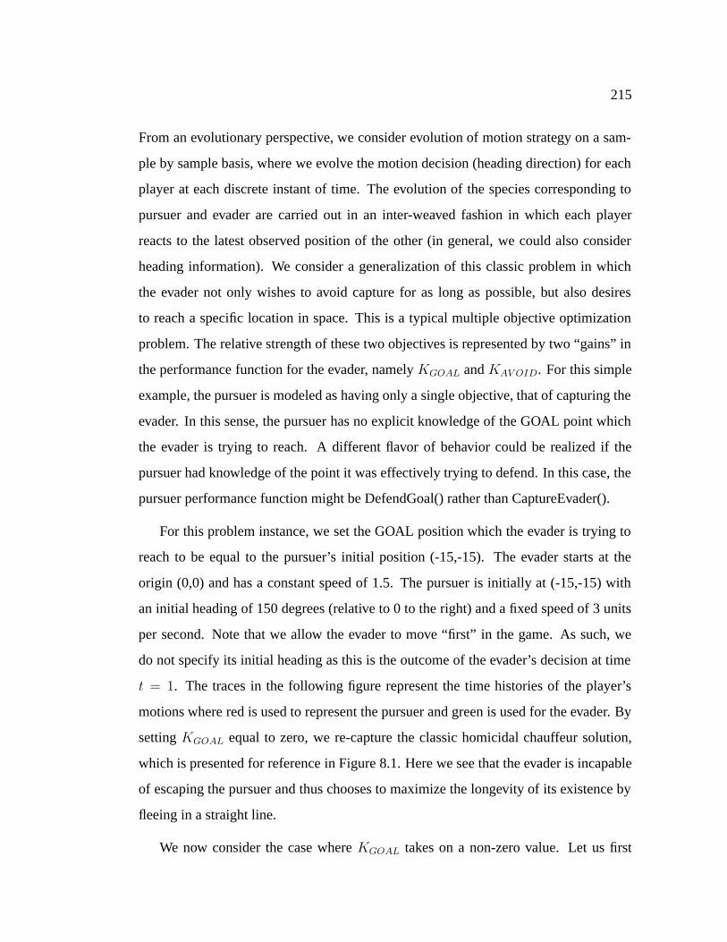
215

From an evolutionary perspective, we consider evolution of motion strategy on a sam-

ple by sample basis, where we evolve the motion decision (heading direction) for each

player at each discrete instant of time. The evolution of the species corresponding to

pursuer and evader are carried out in an inter-weaved fashion in which each player

reacts to the latest observed position of the other (in general, we could also consider

heading information). We consider a generalization of this classic problem in which

the evader not only wishes to avoid capture for as long as possible, but also desires

to reach a specific location in space. This is a typical multiple objective optimization

problem. The relative strength of these two objectives is represented by two “gains” in

the performance function for the evader, namely KGOAL and KAVOID. For this simple

example, the pursuer is modeled as having only a single objective, that of capturing the

evader. In this sense, the pursuer has no explicit knowledge of the GOAL point which

the evader is trying to reach. A different flavor of behavior could be realized if the

pursuer had knowledge of the point it was effectively trying to defend. In this case, the

pursuer performance function might be DefendGoal() rather than CaptureEvader().

For this problem instance, we set the GOAL position which the evader is trying to

reach to be equal to the pursuer’s initial position (-15,-15). The evader starts at the

origin (0,0) and has a constant speed of 1.5. The pursuer is initially at (-15,-15) with

an initial heading of 150 degrees (relative to 0 to the right) and a fixed speed of 3 units

per second. Note that we allow the evader to move “first” in the game. As such, we

do not specify its initial heading as this is the outcome of the evader’s decision at time

t = 1. The traces in the following figure represent the time histories of the player’s

motions where red is used to represent the pursuer and green is used for the evader. By

setting KGOAL equal to zero, we re-capture the classic homicidal chauffeur solution,

which is presented for reference in Figure 8.1. Here we see that the evader is incapable

of escaping the pursuer and thus chooses to maximize the longevity of its existence by

fleeing in a straight line.

We now consider the case where KGOAL takes on a non-zero value. Let us first

216

−20 −15 −10 −5 0 5 10 15 20−20

−15

−10

−5

0

5

10

15

20

x position

y po

sitio

n

initial pursuerposition

initial evaderposition

P E

pursuer and evaderpositions at t = 11

Figure 8.1: Illustration of the classic homicidal chauffeur game in which the evadertries to maximize the time of capture.

examine what happens if KGOAL = 1 and KAV OID = 2. This situation is shown in

Figure 8.2. Note that the evader speed in this example is set to a fixed value of 2 units

per timestep. This is still slower than the pursuer speed which is equal to 3 units per

timestep. Here, because the evader’s behavior is biased toward avoiding the pursuer, it

takes a slow, looping route to the goal and is captured at time t = 16 as indicated.

Alternatively, we can examine the response when we invert the influence of the

behaviors, setting KGOAL = 2 and KAV OID = 1. In this case, the evader is more

strongly attracted to the GOAL and is thus less “afraid” of the pursuer, resulting in the

player traces shown in Figure 8.3. Here we see that the evader motion toward the GOAL

is fast enough to allow it to get inside of the turning radius of the pursuer and thus reach

the GOAL safely. At this point, assuming the game had not ended, the evader could

have stayed within the minimum turning radius indefinitely.

As a last illustration, we consider the behavior resulting from a change in relative

217

−20 −15 −10 −5 0 5 10 15 20 25 30−20

−15

−10

−5

0

5

10

EP

x position

y po

sitio

n

initial pursuerlocation

initial evaderlocation

GOAL

capture attime t = 16

Figure 8.2: Illustration of a goal-oriented version of the classic homicidal chauffeurproblem with KGOAL = 1 and KAVOID = 2.

−20 −15 −10 −5 0 5−25

−20

−15

−10

−5

0

5

GOALE P

x position

KGOAL = 2

KAVOID = 1

Figure 8.3: Illustration of a goal-oriented version of the classic homicidal chauffeurproblem with KGOAL = 2 and KAVOID = 1.

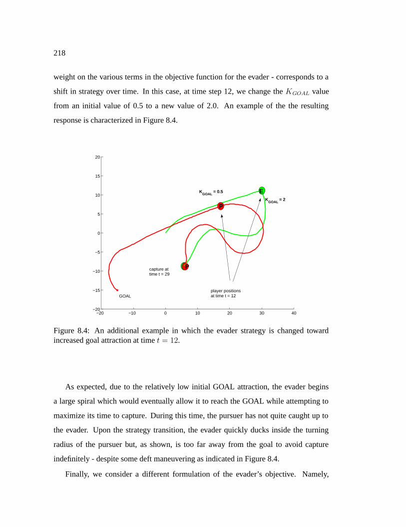
218

weight on the various terms in the objective function for the evader - corresponds to a

shift in strategy over time. In this case, at time step 12, we change the KGOAL value

from an initial value of 0.5 to a new value of 2.0. An example of the the resulting

response is characterized in Figure 8.4.

−20 −10 0 10 20 30 40−20

−15

−10

−5

0

5

10

15

20

GOAL

EP

E

P

KGOAL

= 0.5

KGOAL

= 2

player positions at time t = 12

capture at time t = 29

Figure 8.4: An additional example in which the evader strategy is changed towardincreased goal attraction at time t = 12.

As expected, due to the relatively low initial GOAL attraction, the evader begins

a large spiral which would eventually allow it to reach the GOAL while attempting to

maximize its time to capture. During this time, the pursuer has not quite caught up to

the evader. Upon the strategy transition, the evader quickly ducks inside the turning

radius of the pursuer but, as shown, is too far away from the goal to avoid capture

indefinitely - despite some deft maneuvering as indicated in Figure 8.4.

Finally, we consider a different formulation of the evader’s objective. Namely,

219

rather than trying to maximize her distance from the pursuer, she adopts an avoidance

strategy of “Stay outside of a radius of 5 units” from the pursuer position. Thus, in

the absence of any goal-seeking behavior, one would expect the evader to effectively

do nothing unless the pursuer gets within 5 distance units - at which point, the evader

would attempt to modify its location to satisfy its avoidance objective. We model this

objective using an identical cost function to that used previously. In this case, however,

whenever the distance between the pursuer and evader is greater than 5 units, the corre-

sponding cost component related to avoidance is set to zero. Thus, when the evader is

out of harm’s way, she reverts to goal-seeking behavior, only invoking avoidance when

threatened. For this experiment, we set KAV OID = 4 and KGOAL = 3. The speeds of

the pursuer and evader are set to up = 3 and ue = 2, respectively. Typical behavior

resulting from the simultaneous evolution of strategy in this case is depicted in Figure

8.5.

Here, one observes a dramatic difference in the evader trace as compared with the

previous examples. The evader, rather than heading away from the GOAL, is instead

initially drawn directly towards the GOAL, as it is initially outside of its perceived

threat radius (and is thus safe). The evader then proceeds to execute a series of small

course corrections as indicated. These maneuvers serve to improve its tactical position

by placing it inside the pursuer’s turning radius, running essentially “parallel” to the

pursuer. At time step 12, the evader then takes a quick step to the right, allowing the

pursuer to go by, then hops back to its previous position and proceeds safely to the

GOAL.

8.3 Summary

This chapter has illustrated the use of evolution-based planning to simultaneously evolve

“real-time” (e.g. per decision) strategies for both a pursuer and evader in several types

of differential games. It was demonstrated that this approach can result in “solutions”

which are similar to those obtained analytically using classic differential-game theory.

220

−20 −15 −10 −5 0 5−20

−15

−10

−5

0

5

GOAL

x position

y po

sitio

n

evader initial location

P

E

pursuer locationat time t = 14

evader "jukes", stallingfor pursuer to go by

course corrections for improving tactical position

Figure 8.5: Illustration of the change in evader behavior enabled by a change in avoid-ance objective. Cost component gains are set to KGOAL = 3 and KAVOID = 4.

221

Further, the effect of time-varying strategy on the part of the evader (against a fixed pur-

suer strategy) was illustrated. In particular, an alternative evader cost function related

to a heuristic approximation of “safety” was shown to result in rather creative evader

behavior, similar to might be observed in a game of tag. This behavior was not scripted,

but rather emerged naturally through the evolutionary decision process.

222

Chapter 9

MULTIPLE VEHICLE COORDINATED PLANNING

In this chapter we present discussion of various issues related to the coordination of

multiple vehicles on a given task. The tasks considered include coordinated rendezvous

and a target coverage problem. We demonstrate the ability of the evolution-based plan-

ner to successfully evolve solutions to these types of problems.

9.1 Coordinated Rendezvous

A simple example of multiple vehicle planning is the coordinated arrival at a specified

location. There are two options available for determining the arrival time. It can either

be specified by a mission commander as a fixed time, or can be negotiated by the various

players. We consider the arrival time as determined a priori by some external source.

The population representation we utilize for this example is the maneuver sequence

discussed previously in Chapter 4. We model the decision space of maneuvers at each

point in the sequence as integers in the range [1,5], as defined by the top five rows of

Table 4.3. The application interval for each maneuver is taken as a continuous variable

in the range [0,5]. The vehicle speed is bounded in the range [1,3] with the maximum

change in speed over a given interval limited to 1/sec2. The turn rate within a maneuver

is similarly limited to 30/sec.

We define initial states for a team of three vehicles (labeled A, B, and C) and allow

the evolutionary algorithm to proceed to find routes which enable the team to converge

at a specified point (28.0, 0.0) at the desired time (t = 45 secs). The results of this

simulation are shown below in Figure 9.1. Here we see that the vehicles do indeed reach

the specified location simultaneously as desired. The performance function used in this

223

case was simply the minimization of distance between the vehicle and GOAL location

at the rendezvous time. Note that the vehicles happen to have arrived on approximately

the same “vector” toward the GOAL. This was a coincidence in that no specific penalty

or reward was included in the performance function for the purpose of aligning the

vehicles relative to the GOAL location. This could be trivially included, however, in

order to constrain the arrival to a particular pattern, as might be necessary to optimize

the number of viewed angles, for example (e.g. automatic target recognition).

−30 −20 −10 0 10 20 30 40 50−50

−40

−30

−20

−10

0

10

20

30

40

50

gen: 48

x position

y po

sitio

n

B

A

C

GOAL

Figure 9.1: Coordinated rendezvous at a target.

In the next example, shown in Figure 9.2, we again utilize the maneuver formulation

to generate paths for coordinated engagement of a specified target. The objective is to

nominally arrive at the target at a rendezvous time of 35 seconds, engage the target, and

then return to the base location. In this case, however, we do not allow the vehicles

to approach the target arbitrarily. Rather, we define specific points (at a radius of 5

units from the target center) at which the vehicles must arrive by the rendezvous time.

224

Further, we explicitly penalize collisions between vehicles.

The three vehicles in the team start at the specified locations at arbitrarily chosen

initial speeds and orientations. For the purposes of collision detection, each vehicle

is modeled as a disk of unit radius. The evolved trajectories after 100 generations are

shown in Figure 9.2. The circles shown in Figure 9.2 indicate the vehicle position at

the rendezvous point. Each “dot” along a trajectory corresponds to the vehicle position

at one second intervals. Details of the maneuvering in the vicinity of the target (Figure

−40 −30 −20 −10 0 10 20 30 40 50−40

−30

−20

−10

0

10

20

30

40

x position

y po

sitio

n

base location

target location

aircraft 2 initial posn



Figure 9.2: Solution obtained by EP planner after 100 generations for coordinated ar-rival of 3 vehicles and then return to base.

9.3) highlight the complex behavior that emerges through evolution. In the detailed

view, Vehicle 2 (red) makes a first pass, engaging the target and leaving the engagement

area by t = 35 seconds. Next to pass through the engagement zone is Vehicle 3 (green)

which engages the target and then proceeds to enter a spiral maneuver. This maneuver

effectively allows Vehicle 3 (green) to clear the area for Vehicle 1 (blue) who follows

with a perimeter strike. Finally, Vehicle 3 (green) makes a final pass through the target

area in what might be interpreted as a battle damage assessment role. Note that this

225

20 25 30 35 40

10

5

0

5

10

x position

y po

sitio

n aircraft 3 (t = 35)

aircraft 2 (t = 35)

(t = 40) (t = 40)

(t = 40)

engagement zone

aircraft 1 (t = t 1 (t = 35)ft 1 (t = 3

Figure 9.3: Detailed behavior in the vicinity of the target.

emergent behavior was not “forced” through the objective function. In this case, the

objective function merely consisted of reaching the engagement area by the nominal

rendezvous time and then returning to base.

9.2 Coordinated Coverage of Targets

In this section we consider a target “coverage” problem in which a set of M vehicles

must observe N targets. There are several variations to this problem. In one case, it

might be desirable to minimize the overall mission completion time. Another problem

might be to maximize the value of the overall mission with the requirement that the

vehicles reach the base at a particular time.

A key question to be addressed relates to the overall architecture: whether a single

evolutionary algorithm (EA) should be used for all vehicles or whether separate EAs

should be used for each vehicle. In the latter case, it would be necessary to include some

226

means of communication between the EAs so that information regarding the relative

vicinity of the individual vehicles to particular targets could be shared. This would

eliminate duplicate coverage, ensuring that each vehicle would observe a unique set

of targets. Before delving into one possible solution to this problem, we motivate the

nature of the solution desired through an analogy.

9.2.1 Analogy to Basketball

As a step toward solving this larger problem, we look to analogies which exhibit the

features with which we are most concerned. Namely, we want to identify and distribute

vehicles (e.g. in units of individuals, small groups, or larger swarms) in such a fashion

as to nearly optimally achieve a set of objectives. Note that the objective may not be

a static quantity, but rather may change instantaneously and often over the course of a

given “game”. Here, we look to the game of basketball to provide some insight as to

the desired characteristics we wish our automata to exhibit.

To begin, we consider the “view from the press box” or “eye in the sky” - similar

to a coach who has available a global view of the action in the game. This external,

global view allows the coach to identify patterns and spot anomalies that are perhaps

indetectable at the individual “player” level - either due to a lack of global perspective

or due to a level of complexity which cannot be unraveled. In fact, humans are gen-

erally unequalled in their ability to “filter out” background noise and discern patterns.

The flow of the game of basketball is such that the teams alternately play offense and

defense with the high-level goals of scoring or stopping the other team from scoring,

respectively. The intangible that the coach provides is the mechanism for transform-

ing these high-level objectives into a scheme which is then “learned” by the players

to handle the different situations of play as the arise. These schemes take the form of

“patterns” which are used and transitioned between depending on the state of the game.

They are developed based on the coach observing the strategy of the opposing team

(e.g. on film or based on experience) and abstracting out a mechanism for counter-

227

ing different strategies. The players obviously handle the details of implementing the

“plays” or “patterns” and adjusting the pre-planned motion “algorithms” as necessary

to compensate for the competitor’s actual moves which differ from the “film”.

Typically a basketball team consists of a center, two guards, a forward, and a wing-

man. Associated with each player is a particular role that they typically assume, de-

pending on whether on offense or defense. For a given “play”, each player knows

their role in the pattern. Of course, at various points in the game, each player might

be required to exhibit the characteristics of each role as dictated by the course of play

in order to help out a teammate who might be out of position. Additionally, they are

continually monitoring for certain predicates such as “look for open player”, “maintain

passing lanes”, etc. The players must also know how their roles change as the effective

mode of play on each side changes, ranging from fast break in which the strategies are

“go to basket” and “maintain passing lanes” to full-court press which involves “double-

teaming the ball” and “obstructing passing lanes”. Finally, each player handles the local

navigation and motion planning necessary to carry out their part of each strategy.

9.2.2 Proximity-Based Responsibility

As a preliminary study into multiple vehicle coordinated path planning, the evolution-

ary programming framework was extended to allow for multiple searches to progress

simultaneously. The problem considered consists of path planning for a set of three

vehicles to provide coverage of a set of five randomly placed targets. The mission ob-

jective in this case is simply to visit each observation site and then transit to the base

location. No constraints on the time at which the mission is to be completed are spec-

ified. The architecture chosen for these preliminary investigations incorporates a sep-

arate evolutionary search for each vehicle - with communication between the vehicles

established via the performance evaluation. Essentially the coordinated path planning

problem in this context reduces to a determination of the subset of targets to be associ-

ated with each vehicle as the search progresses. The mechanism used here for handing

228

off or “trading” targets between the vehicles is based on path proximity. For example,

consider Figure 9.4 which shows paths emanating from three vehicles.

A

1

2

3

4

B

C

(1,2)

(3)

(4)

Figure 9.4: Initial implementation of target association based on proximity of trialpaths.

The minimum distance between any of these paths and the targets is noted, with the

corresponding targets being “assigned” to the different vehicles as indicated. The com-

putation of this minimum distance is carried out in a brute force fashion using equation

(5.4). Each vehicle’s trial paths are evaluated based on the set of targets they are cur-

rently closest to. Thus, the individual EP searches accrue target range error penalties

only for those targets it is currently trying to reach. In general, this set of targets can

change with each generation.

As desribed above, the initial implementation used for the simultaneous evolution

of trial paths for multiple vehicles utilized a target assignment scheme based solely on

proximity. Each vehicle effectively runs an independent evolutionary algorithm respon-

sible for determining its path through a set of targets with which it is associated. The

overall cost function used for the j th trial solution of the ith vehicle’s EA is then of the

form:

f(xi,j) = Wττ(xi,j)

+WGR(xi,j [N j ], Gi[N j ]

)(9.1)

229

where τ(·) is the cumulative minimum range error to the set of targets closest to the ith

vehicle during the current generation:

τ(xi,j)

=∑q∈Ti

minkR(xi,j [tk], Tq[tk]) (9.2)

A typical result for this type of problem is illustrated in Figure 9.5, in which the

vehicle routes found after just over 100 generations satisfy the target coverage require-

ments of the mission. For this example, the population size is fixed at µ = 20 indi-

viduals. We represent the input vectors using the instruction list formulation, where

changes in speed and heading are implemented using fixed, deterministic changes of

∆u = ±1 and ∆ψ = ±30. Generation of offspring utilizes the standard GA-like

mutation (pmutate = 0.1) and multi-point crossover (pcrossover = 0.7). The number of

crossover points for each individual is chosen independently at random from a uniform

distribution in the range [1,5].

We demonstrate the adaptation of the individual EA searches by dynamically re-

distributing the targets in the environment. We do this twice in succession, waiting for

the trajectories to converge prior to initiating each new target distribution. The routes

resulting from this process are illustrated in Figure 9.6 in frames (a) and (b).

What can be noted from these figures is that, since the cost function does not include

a penalty on PathLength, paths which have no targets associated with them after re-

distribution tend to remain the same - even when the twists and turns present in their

route are no longer needed. Such is the case, for example, in comparing the trajectory

for vehicle 1 between frames 9.6(a) and (b).

We repeat a similar experiment using the maneuver sequence as the basis of the

input representation. The maximum number of active maneuvers is set to = 20 for

each of the µ = 20 individuals. The space corresponding to the application intervals

is confined to integers in the range [1,5]. The initial distribution of targets is identical

to that used at the outset of the previous example. Results obtained for pcrossover =

0.8 and pmaneuver = ptime = 0.2 are shown in Figure 9.7. Interestingly enough, in

230

−30 −20 −10 0 10 20 30

−30

−20

−10

0

10

20

30

x position

y po

sitio

n

S1 S2

S3

GOAL 1

2

3

4

5

Figure 9.5: Multiple vehicle coordinated routing - after only 100 generations, the vehi-cles have distributed targets and reached the common goal point.

−30 −20 −10 0 10 20 30

−30

−20

−10

0

10

20

30

x position

y po

sitio

n

S1 S2

S3

GOAL

1

2

3

4

5

−30 −20 −10 0 10 20 30

−30

−20

−10

0

10

20

30

x position

y po

sitio

n

S1 S2

S3

GOAL

1

2

3

4

5

(a) (b)

Figure 9.6: Frames (a) and (b) illustrate two subsequent adaptations of routes triggeredby re-distribution of observation targets.

231

comparing the trajectories found in this case with those obtained in Figure 9.5 (based

on the instruction list formulation), one finds that they are quite similar in character.

Investigating the adaptation of trajectories to changes in target position, we interactively

move the set of targets in a manner similar to that presented above - the corresponding

modified routes are displayed in Figure 9.8(a) and (b), respectively.

−30 −20 −10 0 10 20 30−30

−20

−10

0

10

20

30

x position

y po

sitio

n

S1 S2

S3

GOAL 1

2

3

4

5

Figure 9.7: Multiple vehicle target coverage problem - using the maneuver sequenceformulation. State of simulation after approximately 200 generations.

9.2.3 Ability-Based Responsibility

The above example has demonstrated spatial decomposition of targets among a set of

vehicle resources in which dynamic sharing of targets takes place solely on the basis

of physical proximity. A more realistic demonstration would include a mechanism

for assessing the ability of a given vehicle to actually reach its set of goals. In the

event that a vehicle’s planner is struggling to find a route to a given target, this target

could be put up for “auction”, allowing the other vehicles to bid on it based on their

individual estimates of reachability. In this fashion, a more natural collaboration can

232

−30 −20 −10 0 10 20 30−30

−20

−10

0

10

20

30

x position

y po

sitio

n

S1 S2

S3

GOAL1 2

3

4

5

−30 −20 −10 0 10 20 30

−30

−20

−10

0

10

20

30

x position

y po

sitio

n

S1 S2

S3

GOAL

1

2

3

4

5

(a) (b)

Figure 9.8: Frames (a) and (b) illustrate two subsequent adaptations of routes triggeredby re-distribution of observation targets. Routes represented using the maneuver se-quence.

form as a means of maximizing the team value. Generalizing this concept, in order

for autonomous adaptation to the environment to be possible, it is necessary to grant

each individual planning system the ability to make decisions regarding its objectives.

If re-prioritization is deemed necessary in order to continue progress, the planner must

be empowered to do so. Further, this re-prioritization on the individual level must

be communicated to any other vehicles working on the same problem such that they

may adjust their own individual objectives to mesh appropriately relative to the overall

team objectives. This allows vehicles to to take up the slack or anticipate a situation

necessitating a similar re-prioritization on their part. This is not unlike the bidding

and negotiation described by Dias and Stentz [65] in their interpretation of multiple

vehicle coordination in terms of a free market economy. Of course, any changes in

mission objectives must also be communicated to a human manager who may ultimately

determine that data or encounter value warrants a potential loss of vehicle and thus

chooses to override the adaptation and force the originally prescribed behavior. On the

233

other hand, the manager may be able to learn something about the environment based

on the adaptation which might guide future decisions.

With no additional constraints imposed, the solution obtained from the proximity-

based formulation is effectively arbitrary - there being no auxiliary conditions placed

on the solution other than it provide coverage of all the targets and result in each of the

vehicles terminating at the goal location. In some sense, the aforementioned problem

is almost ill-defined in the sense that there is little information available to guide the

optimization process. If, however, one introduces additional features such as a limited

fuel supply for each vehicle, different speed ranges and maneuverability, the problem

becomes much more challenging. Other options which serve to better define the nature

of the solution include modification of the objective function to search for shortest

paths, minimum time paths, minimum energy paths, etc.

9.2.4 Generalized MTSP formulation

We have carried out preliminary simulations involving the simultaneous evolution of

paths for several robotic vehicles charged with visiting a set of arbitrarily located target

locations and convening at a common goal location. These preliminary experiments,

however, implemented dynamic target “sharing”/transfer between robots based solely

on a proximity measure - the idea being that various targets be associated with the

vehicles closest to them. However, we did not take into account the reachability of

the various targets relative to their associated vehicles - either in terms of physical

constraints limiting access or in terms of planning difficulty. Thus, we wish to extend

our study of multiple vehicle coordinated path planning to include consideration of the

difficulty in reaching a given target with any given vehicle.

An alternative formulation, given that the goal of the team of robots is to maximize

the coverage of the targets, is to use an aggregate sum of the distances to all targets

over all vehicles as the figure of merit. In other words, rather than scoring the paths on

an individual basis, one could reserve judgement, effectively combining the trial paths

234

from each vehicle prior to assigning fitness.

We consider a coordinated planning problem consisting of N vehicles tasked with

finding a way to visit M target locations and terminate at a single goal location, where

the aggregate distance traveled by the team is minimized. This is an instance of a

multiple traveling salesperson problem (MTSP). The population representation used

for this problem consists of a “string” of length M , corresponding to the number of

target locations that must be covered. Each of the N vehicles has associated with it

a parameter that represents the number of targets which it is responsible for. These

parameters define the responsibility boundaries within a given string, as indicated below

in Figure 9.9.

vehicle A vehicle B vehicle C

"team" individual

numA numB numC

swap

reverse

shift

Figure 9.9: “Team” individual representation for cooperative planning.

A set of trial solutions is initialized by choosing random permutations of the num-

bers 1 throughM and assigning arbitrary responsibility boundaries such thatN1+N2+

· · ·+NM = M . Evolution of this initial population is carried out through the applica-

235

tion of a set of mutation operators that adjust the ordering and boundaries, as indicated

in Figure 9.9. These operators effectively introduce a dynamic exchange of information

between vehicles, allowing different team strategies to be effectively searched in order

to determine a coverage pattern that minimizes the cumulative team traversal distance.

In evaluating a given sequence, the fitness is obtained assuming straight-line travel of

each vehicle from its starting location, through its associated set of targets, and termi-

nating at the goal location. Note that the initial and goal locations are only utilized for

fitness evaluation and are not explicitly included in the population representation. This

representation proves to be very efficient in finding the true optimal solution (as verified

by comparison with exhaustive enumerative search). A typical example is shown below

for a team of three vehicles seeking to optimally cover a set of five targets. The initial

locations of each of the vehicles is depicted by the shaded circles marked with an ‘S’.

As indicated in Figure 9.10, the team evolution found the optimal solution within 10

generations (approximately 1.5 seconds total run time as compared with 31 seconds for

exhaustive search)

We also include examples with N = 10 and N = 20 targets, shown in Figure 9.11

and Figure 9.12. It is noted that for N = 10, approximate computation time was on

the order of 20 seconds. By comparison, computation time for N = 20 targets was

approximately 120 and 200 seconds for the cases with and without obstacles, respec-

tively. In comparing Figures 9.12(a) and (b), one is struck by the similarities in the

paths discovered by the search process. In particular, one can observe the deviations in

the path necessary in the latter case to avoid the obstacles. These path deviations cause

a slight increase in the cumulative path length, as noted in the figures.

9.3 Summary

Preliminary efforts to date have focused on a centralized “team” representation for the

purposes of evolution, as discussed previously. Although this technique has proved ef-

ficient, we recognize that it suffers due to its dependence on centralized computation

236

−15 −10 −5 0 5 10 15−15

−10

−5

0

5

10

15

1

2

3

45

S

G

S

G

S

G

gen: 10

path total: 64.8746

x position

y po

sitio

n

Figure 9.10: Solution of MTSP obtained using evolutionary programming and the“Team” individual concept for cooperative planning.

−15 −10 −5 0 5 10 15−15

−10

−5

0

5

10

15

1

2

3

4

5

6

7

89

10

S

G

S

G

S

G

105.7745path total:

gen: 65

Figure 9.11: Solution of MTSP involving M = 3 vehicles and N = 10 targets -obtained using the “Team” individual concept. Elapsed time for this solution was ap-proximately 20 seconds.

237

−15 −10 −5 0 5 10 15−15

−10

−5

0

5

10

15

1

2

3

4

5

6 7

8

9

10

11

12

13

14

15

16

1718

19

20

S

G

S

G

S

G

gen: 400

path total: 131.3346

−15 −10 −5 0 5 10 15−15

−10

−5

0

5

10

15

1

2

3

4

5

6 7

8

9

10

11

12

13

14

15

16

1718

19

20

S

G

S

G

S

G1

2

3

4

gen: 400

path total: 143.5009

(a) (b)

Figure 9.12: Solution of MTSP involving M = 3 vehicles and N = 20 targets (a)without any obstacles and (b) with four obstacles place at random locations in the envi-ronment.

of plans which are subsequently distributed to the team members. Several alternative

architectures exist to allow more distributed planning to take place. First off, one could

limit the global extent of planning being considered by restricting the team representa-

tion to include vehicles only in the immediate vicinity. Of course, this would assume

that a vehicle outside of the local area could not potentially contribute in some useful

fashion. Another option is to allow each vehicle to compute a global plan (using the

centralized representation) based on its own local perspective. The idea here is that

each automaton would determine its own duties in the context of what it knows about

the other vehicles. Of course, this alternative is less desirable for several reasons. First,

it does not really distribute the planning effort, but rather duplicates it over each vehicle

in the team. Second, it still depends on a centralized conflict resolution manager which

must receive the global plans from each of the vehicles to sort out potential conflicts or

duplication of effort. What one really desires is a true distributed planning architecture

in which the individual vehicles plan their routes in their own best interest with the re-

sult that the overall team benefits. This is the idea behind a market analogy in which

238

vehicles effectively bid and negotiate for each of the sub-tasks [8]. Given a certain sub-

task (e.g. “observe target 3”), each vehicle which is aware of the presence of target 3

generates a trajectory which allows it to accomplish the task along with the associated

cost in doing so. It is assumed that accomplishing the sub-task brings with it a certain

profit, which serves to benefit both the individual and the team as a whole. Thus the

objective is to assign the sub-task to the automata which can achieve the task at the min-

imum expense, just maximizing the revenue from the transaction. At this point, one can

imagine that the sub-task has associated with it an agent (this might be, for instance, the

vehicle which “found” the target in the first place). The individual vehicles bid against

one another for the sub-task. In particular, the agent compares the cost of doing the

job itself with that received from each of the vehicles. One of the aspects we wish to

explore is the marriage of this market-based analogy which is useful for real-time allo-

cation of tasks with planning. In other words, to study the potential gains to be had if

one can virtually explore potential collaborations prior to execution.

In some sense, one can think of cooperative planning as a multi-objective optimiza-

tion problem in which, in trading off tasks between team members, it is desired to in-

crease the team profit without jeopardizing that of any of the individuals. There are two

basic approaches in solving this problem. In one case, we can consider the shopping

“bag” of each team member to be initially empty. The known targets are then “uncov-

ered” one at a time and presented to the team. The team then commences arbitration

to determine which vehicle should “pick up” the target (based on maximizing individ-

ual revenue). This process continues until all known targets have been assigned. An

alternative approach is to fill the shopping “bags” of each vehicle or “team” randomly

and then allow the market forces to enable trades/purchases/sales of the corresponding

items. This latter approach captures the spirit of the “team” population representation

discussed.

239

Chapter 10

IMPLICATIONS FOR REAL-TIME, REAL-WORLD PLANNING

In the previous chapters, we have demonstrated the ability of an evolution-based

planner to discover trajectories of high utility in both static and dynamic environments.

Throughout these examples, however, it was tacitly assumed that the planner had at its

disposal full information regarding the environment and the motion of various actors

within that environment. In addition, the planner was never under any time pressure to

deliver a solution - it simply was allowed to search until finding a suitable trajectory.

Thus, we now explore the implications of using simulated evolution as the basis for

real-time, real-world planning with time constraints and incomplete information. In

particular, we discuss the relationship between the planning horizon and the global

utility of the evolved trajectories.

10.1 Structure for Real-Time Planning

We begin out discussion of real-time planning by assuming the existence of an initial

feasible trajectory, computed off-line prior to execution. Since this path is computed

off-line in a bounded yet arbitrarily large amount of time, it will generally satisfy the re-

quirements of the mission as defined by the various performance objectives. Of course,

the utility of this path is based solely on information available to the planner prior to

execution. As such, if this trajectory is blindly followed, it is likely that considerable

reduction in utility will occur as the vehicle encounters an environment which fails to

match that assumed in the off-line planning process. Thus the need to be able to adapt

the vehicle’s trajectory on-line while it is in motion.

It is inevitably the case that, despite the availability of faster and faster computa-

240

tional resources, there will always be situations where the vehicle will encounter unan-

ticipated features of the environment faster than the adaptive planner can respond. In

other words, the planner bandwidth is limited - any events that happen outside of this

bandwidth simply cannot be reacted to in time. For this reason, deliberative (look-

ahead) planning alone is not sufficient for control of an autonomous vehicle. In the

limit, one can consider determining the course of action for the next instant of time

based solely on the information available at the current instant. This is the role played

by so-called reactive behaviors [5], a set of high-bandwidth responses to events outside

of the planner bandwidth. These reactive behaviors represent tight, fast loops connect-

ing sensors to actuators, with very little processing in between. Examples for mobile

robots include basic obstacle avoidance or wall-following behavior.

This “library” of basic reactive behaviors can be extended to include goal seeking

behavior - where the vehicle moves towards the goal when possible and avoids obsta-

cles otherwise [6]. This can be thought of as a sort of summation of forces from each

contributing factor (similar to potential field methods, [9]) where forces of attraction

are emitted from goals and forces of repulsion are emitted from obstacles. It is known,

however, that these potential field methods are also subject to the problem of local min-

ima when forces sum to zero in various places in the topology. When this occurs, the

vehicle tends to get “stuck” - in the absence of any net force for local guidance. By

the same token, because reactive behaviors act only on the information available at any

given time, they tend to be exhibit inefficient behavior. This occurs in situations where

multiple behaviors “compete” for control of the vehicle’s action, causing the robot to

wander or hesitate. Further, navigation based on purely reactive strategies is incapable

of utilizing non-sensor based information about the environment such as maps or “in-

telligence” regarding distant threat locations or environment dynamics. Thus, a hybrid

approach to autonomous vehicle control is necessary.

In order to make this idea more concrete, consider Figure 10.1 which shows a ve-

hicle (at time Tc) moving along a nominal feasible trajectory, indicated by the shaded

241

solid line. We define a spawn point, located a time Ts > Tc from the current vehicle po-

initial feasible path

committed section(reactive only)

free/evolving section(t > T s)

current vehiclelocation, x[ T c ]

spawnpoint

(Ts > Tc)

planninghorizon

Figure 10.1: Illustration of concept of adaptive real-time search.

sition along this nominal trajectory, indicated by the black diamond. This spawn time is

directly related to the planning bandwidth and represents an estimate of the maximum

time available to the planner to update the trajectory for tk > Ts. In other words, the

portion of the trajectory for Tc ≤ tk ≤ Ts is assumed committed to execution, being

altered perhaps only by the influence of local reactive behaviors. The path downstream

of the spawn point is taken as free to be further refined or adapted. In this manner, the

planner can naturally account for new information that becomes available regarding the

spatial and temporal state of the environment. There are several options in terms of the

instantiation of the spawn point. One implementation sets the spawn point at a constant

time interval, ∆tspawn = const ahead of the current vehicle location. In this case, the

242

spawn point would be continually updated as the vehicle moves and the length of the

committed portion of the trajectory would remain constant over the length of the mis-

sion. An alternative approach would be to allow the spawn point to remain fixed for a

certain interval, ∆tmax of time while the vehicle moves along the nominal path toward

it. When the vehicle enters within a certain time interval of the spawn point, ∆min, the

spawn point is then reset to a position ∆max ahead of the current position. This latter

method has the advantage of allowing more planning time to be allotted to the region

of the trajectory in the immediate vicinity of the spawn point.

Regardless of its implementation, real-time delivery of trajectories to the vehicle

control system requires the introduction of time available for planning as an additional

constraint on the planning process. This additional constraint has an immediate influ-

ence on the cost function used for evaluating trial paths. During intervals in which

the time for planning is abundant, the priorities represented in the cost function can

be biased toward optimizing performance and satisfaction of long-term goals. As the

urgency to deliver a plan increases, the priorities in the cost function must necessarily

be shifted toward delivering feasible solutions which enable the vehicle to keep moving

in at worst a zero-loss manner (e.g collision free, avoiding risky behavior, etc.). Once

the motion plan is updated and the planner window expands, the goal priorities can be

reset to the longer-term objectives.

An obvious consideration in this formulation is the extent of the planning horizon,

or how far ahead of the spawn point the planner looks. Ideally, one could plan the

entire remainder of the mission from Ts ≤ t[k] ≤ t[] within the time available. In

this fashion, one could guarantee that all downstream factors are considered in making

local shaping decisions, hedging the probability of discovering more globally optimal

solutions. Further, as the mission progresses, the temporal extent of planning required

continually decreases until finally the last portion of the mission is committed to exe-

cution. This ability, however, is impractical for realistic problems involving missions

of long duration (on the order of hours) due to the computation effort required and the

243

degradation in certainty in the data with increasing time. There is a point of diminishing

returns in terms of the tradeoff of value against computational effort.

These considerations lead one to envision a planning architecture in which several

planners operate simultaneously, running as separate processes:

1. a low bandwidth planner which updates every hour the entire remainder of the

mission,

2. a medium bandwidth planner which updates the motion plan for the next hour

every ten minutes, and

3. a high-bandwidth planner which updates the next ten minutes of the trajectory

every minute.

10.2 Planning with Incomplete Information

The previous section addressed the design of an architecture for real-time planning for

an individual vehicle. Implicit in this design, however, is the assumption of the avail-

ability of data regarding the time-varying state of the environment. Such information

may be provided, for example, in the form of a set of gridded databases. In this fashion,

the grid point value (e.g. wind speed) at a given location and future time can be at least

approximately computed by interpolation between the various data sets. In actuality,

however, such data may be only scarcely available or may not be available directly at

all. Even if such data is available, it will inevitably contain both spatial and temporal

uncertainty. For example the wind intensity at a given location might vary in speed

and/or heading. Ideally, one could take this uncertainty into account in order to find

trajectories with a high probability of being successful. One mechanism for doing so

would be to plan a series of trajectories over various worst-case scenarios and using

some sort of blending scheme to combined these trajectories based on the actual values

sensed during execution.

244

In terms of sources of data, often times the vehicle itself (via its sensors) is the

most reliable source at a given point in time. Typically, however, it is the downstream

(i.e. separated in “time” or distance) estimates of the future state of the environment

which are of most concern. Unfortunately it is often the case that information at loca-

tions where we are not is more valuable that that at our current location. This is the

advantage of teams of automata distributed spatially through an environment. By co-

ordinating their sensor readings, they can share with one another their own individual

views to form a uniform shared composite view of the environment. This has the effect

of drastically reducing at least the spatial uncertainty in data. Obviously, temporal vari-

ations in the environment will tend to increase uncertainty to a certain extent. Thus, it is

assumed that each robot in a team keeps an internal representation of the environment.

These representations, initially identical prior to execution, are modified through the

personal experience of each member of the team (e.g. unique sensor capabilities and

exposure to different parts of the environment). This unique experience allows each

robot to contribute to a shared “mental model” of the environment in situations where

communication between robots is not limited. Planning is predicated on the existence

of internal models of both the environment as well as the robotic system itself. On-

line learning, based on experience, is used to continually update these models during

execution. In this manner, the planning algorithms have access to the best available

information (as well as estimates of uncertainty) in making decisions regarding future

courses of action.

Such data may be developed based on external detailed ground-based computation

(e.g. atmospheric models) or might be derived based on sensor information obtained by

other systems (e.g. satellite imagery, databases, humans, or robotic vehicles). Thus, a

practical concern is the dissemination of data throughout the virtual network - whether

this network consist of a single or multiple vehicles. Questions which must be an-

swered include the types of information which need to be distributed, the frequency at

which communication must take place, and the required topology of the network. In

245

other words, is it necessary for each vehicle to talk to each other node of the network

or is a proxy or relay system adequate? Does this communication happen at a fixed

rate or sporadically as the situation dictates? Limited communication (due to stealth re-

quirements, security concerns, or simply lack of bandwidth or line-of-sight) inevitably

impacts the quality of plans which can be created as the planner is required to act on an

incomplete picture or “mental model” of the environment and the intent of the various

actors within that environment.

10.3 Toward Semi-Autonomous Vehicles

In this section, we re-visit the role of planning in the overall vehicle control system. We

do so from the perspective of highlighting the requirements which enable autonomous

robotic systems to work together with human counterparts to solve problems.

As described throughout this dissertation, operations in dynamic real-world envi-

ronments, wrought with uncertainty, require robotic systems to continually adapt their

behavior in the face of unanticipated changes in order to continue to carry out their mis-

sion to the extent possible. Such adaptation may be triggered, for example, by sensed

discrepancies between the vehicle’s internal representation and the actual environment,

vehicle or communication failures, or a detected inability to achieve its goal(s). In

the extreme, it may be necessary to redefine or re-prioritize the objectives of the orig-

inal mission - thus the motivation for explicitly taking a multi-objective approach to

the planning problem. True autonomy implies the ability for this adaptation to occur

without direct human intervention. A semi-autonomous system allows the human to

establish and manage the objectives for the system and participate in the planning at

will while removing the need for direct control.

Given a high-level objective such as “Clear that building and search for survivors”

or “Follow that vehicle, but stay high to avoid being detected”, it is up to the individual

or team of robots to:

246

1. Resolve any ambiguity in the syntactical parsing and interpretation of the stated

objective

2. Transform the objective into a set of sub-tasks to be accomplished

3. Determine the mapping of individual robots to sub-tasks

4. Decide the ordering (if any) in which the tasks are to be completed

5. Develop detailed plans for each of the individual robots in accomplishing each of

their assigned tasks

6. Account for possible collaboration between robots taking advantage of different

resources and capabilities and resolve potential conflicts

Of course, this list does not represent a single-pass process. Rather, the various items

must really occur simultaneously (possibly as separate processes) on-board the individ-

ual or team of robots while the mission is being executed. This is necessary to handle

the potential time-varying nature of the mission objective(s), the environment, and the

vehicle’s themselves (e.g. failures). We reiterate that a key feature implied by the no-

tion of semi-autonomy is the ability of the human to intercede at any given level of

processing and computation. The level of autonomy granted to the robotic systems is

therefore adjustable and time-varying, depending on the needs and constraints imposed

by the evolving mission.

Note that this dissertation has focused on a limited sub-set of the tasks listed above.

Namely, we have demonstrated the viability of an evolution-based planner in devel-

oping detailed action plans, where action is interpreted in the context of sequential

motion decisions. It is emphasized, however, that the results obtained thus far, al-

though promising, really only represent the tip of the iceberg in terms of the long-term

potential for these techniques. In fact, the sequential decision formulation developed

247

in this research can not only handle the detailed low-level planning (Task 5), but can

quite readily be extended to handle the higher-level optimization implied by Tasks 3-4

as well. This follows from a generalization of the “team” representation described in

Chapter 9. This team representation would be utilized at the highest level of abstraction,

making decision regarding the fitness of different task distributions based on the output

of additional (potentially evolution-based) search taking place at lower levels. Such an

architecture implies the existence of either explicit (through direct communication) or

implicit (through sensing of the environment) feedback among the search algorithms

processing information at the various levels of abstraction.

248

Chapter 11

CONCLUSIONS

In this chapter, we summarize the main results and make suggestions for future

research.

11.1 Summary of Work

This research began in the context of developing adaptive path planning algorithms for

air vehicles flying missions requiring significant duration (on the order of hours). Ini-

tially, approaches based on variational calculus and dynamic optimization were investi-

gated and found to be infeasible for on-line planning due to the excessive time required

for solution. Heuristic approaches to traveling salesperson problems (TSP) were then

explored. While these algorithms efficiently find near-optimal orderings of target or

goal points, they fail to provide any information regarding the details of how to get

between the points. As a first step toward filling this gap, graph search techniques (dy-

namic programming, A∗, etc.) were studied and found to be capable of finding optimal

spatial solutions to “shortest path” type problems over discrete graphs. Shortcomings

of these algorithms, however, include their inability to determine speeds between the

nodes of the graph and the complexity involved to get them to handle time-of-arrival

constraints at particular goals. Further, although these algorithms can be modified to

solve problems involving multiple goals, they require the use of a separate combinato-

rial optimizer for the purpose of higher-level mission goals.

Rather than making decisions on a time-step by time-step basis, we propose the use

of evolutionary algorithms for the generation of “look-ahead” motion plans. Depending

on the search horizon used, these algorithms allow future actions to be evaluated based

249

on an estimate of the environment within which these future decisions are made.

We have found evolution-based planners to be effective at finding high utility routes

through generally open environments containing both static and dynamic obstacles and

target locations.

We have shown that, given appropriate population representations and mutation

strategies, an evolution-based planner can:

1. Efficiently search complex multi-dimensional search spaces (mixed continuous

and/or discrete in nature)

2. Handle performance functions of arbitrary complexity and form (e.g. not hin-

dered by smoothness/differentiability requirements)

3. Naturally include hard constraints (e.g. collision and threat avoidance)

4. Include a mix of robotic platforms with differing dynamics (e.g. land, sea, air,

non-holonomic)

5. React to impaired performance resulting form battle damage and quickly generate

alternative courses of action

6. Incorporate intelligent adversaries (e.g. differential games) through simultaneous

evolution of both friendly and enemy strategies

11.2 Improvements for Real-Time Implementation

The investigations with the evolution-based planner to date have been largely proof-

of-concept studies to establish the viability of simulated evolution as an adaptive path

planning process. As such, little effort has been made to streamline the search process

for the purposes of real-time operation.

250

11.2.1 Efficient Collision Detection

A majority of the computational loading (approximately 70 − 80%)of the current im-

plementation involves the estimation of collisions through obstacle penetration values,

based on the intersection of minimally enclosing rectangles bounding the various “bod-

ies” in the simulation. These values are utilized in order to avoid hard constraints as

well as maintain adequate separation in multiple vehicle simulations. For a single vehi-

cle maneuvering throughM obstacles, this computation requiresO(MNi) comparisons

per path at each generation, where N is the number of segments in the ithpath. This

computational effort grows exponentially with the number of vehicles in the simula-

tion. Thus, it is desired to find mechanisms for reducing the computational burden of

collision detection. Recall, however, that we desire not only a binary indicator of col-

lision but a semi-continuous variable indicating the “degree” of collision. This degree

of penetration effectively as a “gradient” to allow the evolution to find alternative mo-

tion strategies around obstacles. Without this information, it is difficult to differentiate

between really deep collisions and those paths which are nearly collision-free.

One way in which the collision computation can be reduced is to prune the physical

environment of the simulation in some fashion, such as using a quadtree to break the

whole environment into a number of separate sections. In this manner, detailed col-

lision checks only have to be done between bodies within the same section, avoiding

unnecessary computation between bodies that could not be colliding. It should be in-

vestigate the impact that this and other concepts from computational geometry might

be used to reduce the cost of collision detection.

11.2.2 Avoiding Duplication of Effort

Recall that evolution-based search is fundamentally a “generate and test” approach to

planning in which a large number of potential future action plans are generated in paral-

lel. Each potential action plan is then assessed as to the degree to which it accomplishes

the mission objectives while satisfying the mission constraints. Because this generation

251

process is random, it is often the case that candidate solutions, previously judged to have

poor fitness, will be “rediscovered” many times. To prevent this duplication of effort,

one could imagine keeping track of each candidate solution which is generated such

that any future duplicates are thrown away without any computational effort expended

in its evaluation. Note that without a one-to-one mapping between the instruction list

and paths would make such a decision impossible. Of course, depending on the size

of the search space and the number of generations involved, the computational effort

required to search this history “buffer” would quickly surpass that needed to evaluate

the path in the first place. Further, since the state of the environment is in general time-

varying, there is no reason to think with absolute certainty that a solution previously

judged to have poor fitness might suddenly become optimal based on the current en-

vironment. A compromise solution which should be considered would keep a “local”

(in time) history buffer which acts a sliding window, tracking the enumeration of paths

(or instruction lists) over the last Nhistory generations. This buffer could be “reset”

whenever a significant change in the environment was sensed or otherwise indicated by

external information.

11.3 Suggestions for Future Research

The following topics are suggested as starting points for further research:

• Further generalize the “repulsion” concept introduced in Chapter 6 as a means of

avoiding local minima traps. This is necessary for path planning in more con-

fined areas such as buildings and/or “mazes” where multiple walls separate the

vehicle from the goal. What is needed is a path scoring mechanism which en-

courages exploration of new territory (e.g. maximize along-path distance from

the current position) while avoiding looping behavior (which extends the along-

path distance without significantly changing location). Of course, such domains

are more amenable to discrete space representations or landmarks (e.g. stairs,

252

hallways, doorway locations, etc.) and allowing the local control of the vehicle

(obstacle avoid, wall follow, etc.) to handle navigation between landmarks.

• Evaluate performance relative to uncertain information to find best performance

over a number of likely scenarios

• Further develop applications of simultaneous evolution of strategy in multi-player

games. In particular, utilize a set of battle dynamics to evolve force allocation and

deployment (air tasking) in simulated war games.

• Investigate cooperative co-evolution as a mechanism for coordinating motion

plans and action strategies between multiple autonomous vehicles cooperating

on a given task

• Investigate the potential for evolution-based methods to not only develop the de-

tailed plans given a mapping of vehicles to tasks, but also to develop this mapping

in the first place. At this level of abstraction, optimization would be over the set

of available platforms, resources, and high-level task descriptions.

• Develop an integrated, multi-layer evolution-based mission planning and man-

agement algorithm. Study the interaction of evolution at a number of different

levels simultaneously. Each layer has its own population dynamics, but there

needs to be communication through the hierarchy to transmit strategy updates

at each individual layer. These decisions, based on “experience” gained at the

individual level, potentially influence future decisions at both higher and lower

levels. Some of this information may be observable indirectly through sensing of

the environment rather than through direct communication.

• Combine a deliberate, forward-looking evolution-based planner with a machine

learning strategy (e.g. reinforcement learning) for evolving reactive behaviors.

253

BIBLIOGRAPHY

[1] “Unmanned Aerial Vehicles Roadmap, 2000-2025.” Office of the Secretary

of Defense, April 2001. Available at http://www.acq.osd.mil/acqweb/usd/uav

roadmap.pdf.

[2] P. Antsaklis, K. Passino, and S. Wang, “Towards intelligent autonomous con-

trol systems: Architecture and fundamental issues,” Journal of Intelligent and

Robotic Systems, vol. 1, pp. 315–342, 1989.

[3] D. W. Payton et al., “Do Whatever Works: A Robust Approach to Fault-Tolerant

Autonomous Control,” Journal of Applied Intelligence, vol. 2, pp. 225–250,

1992.

[4] D. W. Payton, “Internalized plans: A representation for action resources,”

Robotics and Autonomous Systems, vol. 6, pp. 89–103, 1990.

[5] R. A. Brooks, “A Robust Layered Control System for a Mobile Robot,” IEEE

Journal of Robotics and Automation, vol. RA-2, pp. 14–23, March 1986.

[6] T. Balch and R. Arkin, “Avoiding the past: a simple but effective strategy for

reactive navigation,” in Proc. 1993 IEEE International Conference on Robotics

and Automation, (Atlanta, GA), pp. 678–685, May 1993.

[7] R. Arkin and T. Balch, “Cooperative multiagent robotic systems,” 1998.

[8] M. Schoppers, “Universal plans for reactive robots in unpredictable environ-

ments,” in Proceedings of the 10th International Joint Conference on Artificial

Intelligence (IJCAI-87), (Milan, Italy), pp. 1039–1046, 1987.

254

[9] O. Khatib, “Real-Time Obstacle Avoidance for Manipulators and Mobile

Robots,” The International Journal of Robotics Research, vol. 5, no. 1, pp. 90–

98, 1986.

[10] J. T. Betts, “Survey of numerical methods for trajectory optimization,” Journal

of Guidance, Control, and Dynamics, vol. 21, pp. 193–207, March-April 1998.

[11] D. W. Miles and S. M. Rock, “Real-time dynamic trajectory optimization,” in

Proceedings of the AIAA Guidance, Navigation and Control Conference, (Re-

ston, VA), pp. 1–9, July 1996. AIAA-96-3741.

[12] J. Vian, S. J. Fu, D. L. Grose, and M. Sawan, “Intelligent flight management in

threat environments,” in Proceedings of the IEEE 1988 National Aerospace and

Electronics Conference, pp. 224–228, 1998.

[13] M. B. Milam, K. Mushambi, and R. M. Murray, “A new computational approach

to real-time trajectory generation for constrained mechanical systems,” in 39th

IEEE Conference on Decision and Control, (Sydney, Australia), December 2000.

[14] J. S. Mitchell, D. W. Payton, and D. M. Keirsey, “Planning and reasoning for

autonomous vehicle control,” International Journal of Intelligent Systems, vol. 2,

pp. 129–98, 1987.

[15] J. S. Mitchell, “An algorithmic approach to some problems in terrain navigation,”

Artificial Intelligence, vol. 37, pp. 171–201, December 1988.

[16] D. Keirsey, J. Mitchell, D. Payton, and E. Preyss, “Multilevel path planning for

autonomous vehicles,” in Proceedings of the SPIE Conference on Applications

of Artificial Intelligence, vol. 485, (Arlington, VA), pp. 133–137, 1984.

255

[17] J. S. Mitchell and D. M. Keirsey, “Planning strategic paths through variable ter-

rain data,” in Proceedings of the SPIE Conference on Applications of Artificial

Intelligence, vol. 485, (Arlington, VA), pp. 172–179, 1984.

[18] J. S. Mitchell, “An autonomous vehicle nagivation algorithm,” in Proceedings of

the SPIE Conference on Applications of Artificial Intelligence, vol. 485, (Arling-

ton, VA), pp. 153–158, 1984.

[19] J. Krozel, “Search problems in mission planning and navigation of autonomous

aircraft,” Master’s thesis, Purdue University, West Lafayette, IN, May 1988.

[20] J. Krozel and D. Andrisani, “Navigation path planning for autonomous air-

craft: Voronoi diagram approach,” Journal of Guidance, Control and Dynamics,

pp. 1152–1154 (Engineering Notes), Nov-Dec 1990.

[21] J. A. Sorensen, “The flight planning - flight management connection,” in Pro-

ceedings of the 1984 American Control Conference, vol. 1, pp. 174–178, 1984.

[22] J. A. Sorensen and T. Goka, “Design of an advanced flight planning system,”

in Proceedings of the 1985 American Control Conference, vol. 2, pp. 663–668,

1985.

[23] J. Wilson, C. Wright, and G. J. Couluris, “Advanced free flight planner and dis-

patcher’s workstation: Preliminary design specification,” Tech. Rep. NASA Con-

tract NAS2-14289, Seagull Technology, Los Gatos, CA 95032-2547, November

1997.

[24] J. Krozel, C. Lee, and J. S. Mitchell, “Estimating Time of Arrival in Heavy

Weather Conditions,” in AIAA Guidance, Navigation and Control Conference

(AIAA paper 99-4232), (Portland, OR), 1999.

256

[25] P. Hagelauer and F. Mora-Camino, “A soft dynamic programming approach for

on-line aircraft 4d-trajectory optimization,” European Journal of Operational

Research, vol. 107, pp. 87–95, 1998.

[26] T. Wilkin, “Personal communication.,” March 2000.

[27] T. Wilkin and A. Nicholson, “Efficient inference in dynamic belief networks with

variable temporal resolution,” in Proceedings of the 6th Pacific Rim International

Conference on Artificial Intelligence, pp. 264–274, Springer-Verlag, 2000.

[28] A. Stentz, “Optimal and Efficient Path Planning for Partially-Known Environ-

ments,” in Proceedings of the 1994 International Conference on Robotics and

Automation, vol. 4, (Los Alamitos, CA), pp. 3310–3317, 1994.

[29] A. Stentz, “The Focussed D* Algorithm for Real-Time Replanning,” in Pro-

ceedings of the International Joint Conference on Artificial Intelligence, August

1995.

[30] P. E. Hart, N. J. Nilsson, and B. Raphael, “A formal basis for the heuristic deter-

mination of minimum cost paths,” IEEE Transanctions of Systems, Science, and

Cybernetics, vol. SSC-4, pp. 100–107, July 1968.

[31] T. Linden and J. Glicksman, “Contingency planning for an autonomous land

vehicle,” in Proceedings IJCAI-87, (Milan, Italy), pp. 1047–1054, 1987.

[32] A. Mandow, L. Mandow, V. Munoz, and A. Garcia-Cerezo, “Multi-Objective

Path Planning for Autonomous Sensor-Based Navigation,” in Proceedings of the

IFAC Workshop on Intelligent Components for Vehicles, pp. 377–382, March

1998.

257

[33] J. L. Bander and C. C. White, “A heuristic search algorithm for path determina-

tion with learning,” IEEE Transactions on Systems, Man, and Cybernetics - Part

A: Systems and Humans, vol. 28, pp. 131–134, January 1998.

[34] R. S. Sutton, “Planning by Incremental Dynamic programming,” in Proceedings

of the Ninth Conference on Machine Learning, Morgan-Kaufmann, 1991.

[35] V. Ablavsky and M. Snorrason, “Optimal search for a moving target: A geo-

metric approach,” in AIAA Guidance, Navigation, and Control Conference and

Exhibit, (Denver, CO), 14-17 August 2000. AIAA-2000-4060, A00-37049.

[36] G. S. Kirk and E. E. Kadar, “Field Theory Based Navigation Towards a Moving

Target,” in Advanced Robotics: Beyond 2000, 29th International Symposium on

Robotics, pp. 153–156, 27 Apr-1 May 1998.

[37] E. Kadar and G. Virk, “Field Theory Based Navigation for Autonomous Mo-

bile Machines,” in IFAC Intelligent Components for Vehicles, (Seville, Spain),

pp. 123–128, 1998.

[38] G. Virk and E. Kadar, “Co-operative navigation for target searching in a diffusion

field,” in Proceedings of the 1998 IEEE International Conference on Control

Applications, (Trieste, Italy), pp. 423–427, 1-4 September 1998.

[39] H. V. D. Parunak and S. Brueckner, “Entropy and self-organization in multi-

agent systems,” in Forthcoming at the International Conference on Autonomous

Agents (Agents 2001), 2001.

[40] H. V. D. Parunak, “”Go to the Ant”: Engineering Principle from Natural Multi-

Agent Systems,” Annals of Operations Research, Special Issue on Artificial In-

telligence and Management Science, vol. 75, pp. 69–101, 1997.

258

[41] S. Brueckner and H. Parunak, “Multiple Pheromones for Improved Guidance,”

in Proceedings of the 2nd DARPA-JFACC Symposium on Advances in Enterprise

Control, (Minneapolis, MN), July 2000.

[42] H. V. D. Parunak and S. Brueckner, “Ant-like missionaries and cannibals: Syn-

thetic pheromones for distributed motion control,” in Fourth International Con-

ference on Autonomous Agents (Agents 2000), (Barcelona, Spain), June 2000.

[43] L. Kavraki, M. Koloutzakis, and J.-C. Latombe, “Analysis of Probabilistic

Roadmaps for Path Planning,” IEEE Transactions on Robotics and Automation,

vol. 14, pp. 166–171, February 1998.

[44] S. M. LaValle and J. J. Kuffner, “Randomized Kinodynamic Planning,” in Proc.

of the 1999 IEEE Int’l Conf. on Robotics and Automation, (Detroit, MI), pp. 473–

79, May 1999.

[45] R. Kindel, D. Hsu, J.-C. Latombe, and S. Rock, “Kinodynamic Motion Planning

Amidst Moving Obstacles,” in Proc. of the 2000 IEEE Int’l Conf. on Robotics

and Automation, (San Francisco, CA), pp. 537–43, April 2000.

[46] E. Frazzoli, M. A. Dahleh, and E. Feron, “Real-Time Motion Planning for Agile

Autonomous Vehicles,” in AIAA Guidance, Navigation, and Control Conference,

(Denver, CO), 14-17 August 2000.

[47] J. M. Ahuactzin et al., “Using genetic algorithms for robot motion planning,”

in ECAI 1992, 10th European Conference on Artificial Intelligence, (London,

England), pp. 671–675, 1992.

[48] E. Mazer, J. M. Ahuactzin, and P. Bessiere, “The Ariadne’s Clew Algorithm,”

Journal of Artificial Intelligence Research, vol. 9, pp. 295–316, November 1998.

259

[49] J. Xiao et al., “Adaptive evolutionary planner/navigator for mobile robots,” IEEE

Transactions on Evolutionary Computation, vol. 1, pp. 18–28, April 1997.

[50] D. Fogel, “An evolutionary approach to the traveling salesman problem,” Bio-

logical Cybernetics, vol. 60, no. 2, pp. 139–144, 1988.

[51] D. B. Fogel and L. J. Fogel, “Optimal Routing of Multiple Autonomous Under-

water Vehicles through Evolutionary Programming,” in Proc. of the 1990 Sym-

posium on Autonomous Underwater Vehicle Technology, (Washington, D.C.),

pp. 44–47, 1990.

[52] J. McDonnell and W. Page, “Mobile Robot Path Planning Using Evolutionary

Programming,” in 24th Asilomar Conference on Signals, Systems, and Comput-

ers, (San Jose, CA), pp. 1025–1029, 1990.

[53] W. Page, J. McDonnell, and B. Anderson, “An Evolutionary Programming Ap-

proach to Multi-Dimensional Path Planning,” in Proceedings of the First Annual

Conference on Evolutionary Programming, (La Jolla, CA), pp. 63–70, February

1992.

[54] P. Vadakkepat, K. C. Tan, and W. Ming-Liang, “Evolutionary artificial potential

fields and their application in real time robot path planning,” in Congress of

Evolutionary Computation, (San Diego, CA), pp. 256–63, July 2000.

[55] M. Adams, O. Deutsch, and J. Harrison, “A hierarchical planner for intelligent

systems,” in Proceedings of the SPIE Conference on Applications of Artificial

Intelligence II, vol. 548, (Arlington, VA), pp. 207–218, 1985.

[56] O. L. Deutsch, J. V. Harrison, and M. B. Adams, “Heuristically-guided planning

for mission control/decision support,” in AIAA conference on Guidance, Control

and Navigation (AIAA paper 85-1909), (Snowmass, CO), pp. 386–395, 1985.

260

[57] R. Beaton, M. Adams, and J. Harrison, “Real-time mission planning and trajec-

tory planning,” in Proceedings of the 26th Conference on Decision and Control,

(Los Angeles, CA), pp. 1954–59, 1987.

[58] J. H. Hino, “Intelligent planning for a search and surveillance unmanned under-

water vehicle,” in Proceedings of the 6th International Symposium on Unmanned

Untethered Submersible Technology, pp. 236–245, 1989.

[59] S. Chien et al., “Aspen - automated space mission operations using automated

planning and scheduling,” in SpaceOps 2000, (Toulouse, France), June 2000.

[60] S. Chien et al., “Using iterative repair to increase the responsiveness of planning

and scheduling for autonomous spacecraft,” in IJCAI99 Workshop on Scheduling

and Planning meet Real-time Monitoring in a Dynamic and Uncertain World,

(Stockholm, Sweden), August 1999.

[61] P. R. Chandler, S. Rasmussen, and M. Pachter, “Uav cooperative path planning,”

in AIAA Guidance, Navigation, and Control Conference and Exhibit, (Denver,

CO), 14-17 August 2000. AIAA-2000-4370, A00-37127.

[62] T. W. McLain and R. W. Beard, “Trajectory Planning for Coordinated Ren-

dezvous of Unmanned Air Vehicles,” in AIAA Guidance, Navigation, and Con-

trol Conference and Exhibit, (Denver, CO), 14-17 August 2000. AIAA-2000-

4369, A00-37126.

[63] B. L. Brumitt and A. Stentz, “Dynamic Mission Planning for Multiple Mobile

Robots,” in Proceedings of the 1996 IEEE International Conference on Robotics

and Automation, (Minneapolis, MN), pp. 2396–2401, April 1996.

[64] B. L. Brumitt and A. Stentz, “GRAMMPS: A Generalized Mission Planner for

Multiple Mobile Robots in Unstructured Environments,” in Proceedings of the

261

1998 IEEE International Conference on Robotics and Automation, (Leuven, Bel-

gium), pp. 1564–1571, May 1998.

[65] M. B. Dias and A. Stentz, “A Free Market Architecture for Distributed Control

of a Multi-Robot System,” in Proceedings of the 6th International Conference

on Intelligent Autonomous Systems, July 2000.

[66] M. D. Bugajska and A. C. Schultz, “Co-Evolution of Form and Function in the

Design of Autonomous Agents: Micro Air Vehicle Project,” in WGECCO-2000

Workshop on Evolution of Sensors in Nature, Hardware, and Simulation, (Las

Vegas, NV), July 8 2000.

[67] A. C. Schultz, “Learning Robot Behaviors Using Genetic Algorithms,” in Pro-

ceedings of the First World Automation Congress (WAC ’94), Intelligent Automa-

tion and Soft Computing: Trends in Research, Development, and Applications,

(Albuquerque, NM), pp. 607–612, August 14-17 1994.

[68] A. S. Wu, A. C. Schultz, and A. Agah, “Evolving Control for Distributed Micro

Air Vehicles,” in Proceedings of the IEEE 1999 Int. Symp. on Computational

Intelligence in Robotics and Automation, (Monterey, CA), November 8-9 1999.

[69] B.-T. Zhang and S.-H. Kim, “An evolutionary method for active learning of mo-

bile robot path planning,” in Proceedings of 1997 IEEE International Symposium

on Computational Intelligence in Robotics and Automation (CIRA’97), (Mon-

terey, CA), pp. 312–317, July 1997.

[70] E. Uchibe, M. Nakamura, and M. Asada, “Co-evolution for cooperative behavior

acquisition in a multiple mobile robot environment,” in Proceedings of the 1998

IEEE/RSJ International Conference on Intelligent Robots and Systems, (Victoria,

B.C., Canada), October 1998.

262

[71] S. Luke and L. Spector, “Evolving Teamwork and Coordination with Genetic

Programming,” in Genetic Programming 1996: Proceedings of the First Annual

Conference (J. R. Koza, D. E. Goldberg, D. B. Fogel, and R. L. Riolo, eds.),

(Stanford University), 1996.

[72] F. H. Bennett, “Automatic Creation of an Efficient Multi-Agent Architecture Us-

ing Genetic Programming with Architecture-Altering Operations,” in Genetic

Programming 1996: Proceedings of the First Annual Conference (J. R. Koza,

D. E. Goldberg, D. B. Fogel, and R. L. Riolo, eds.), (Stanford University), 1996.

[73] J. Liu, J. Wu, and Y. Tang, “On Emergence of Group Behavior in a Genetically

Controlled Autonomous Agent System,” in Proceedings of the The 1998 IEEE

International Conference on Evolutionary Computation, pp. 470–475, 1998.

[74] S. D. Patek, D. A. Logan, and D. A. Castanon, “Approximate Dynamic Pro-

gramming for the Solution of Multiplatform Path Planning Problems,” in IEEE

1999 Systems, Man, and Cybernetics Conference, (Tokyo), pp. 1061–66, Octo-

ber 1999.

[75] J. M. Wohletz, D. A. Castanon, and M. L. Curry, “Closed-Loop Control for Joint

Air Operations,” in To appear in Proceedings of the 2001 American Control

Conference, (Arlington, VA), June 2001.

[76] A. C. Schultz and J. J. Grefenstette, “Improving Tactical Plans with Genetic Al-

gorithms,” in Proceedings of IEEE Conference on Tools for Artificial Intelligence

TAI ’90, (Herndon, VA), pp. 328–334, November 6-9 1990.

[77] D. Cliff and G. F. Miller, “Co-evolution of Pursuit and Evasion ii: Simulation

Methods and Results,” in Proceedings of the Fourth International Conference on

Simulation of Adaptive Behavior: From Animals to Animats, (Falmouth, MA),

pp. 506–515, September 1996.

263

[78] C. W. Reynolds, “Competition, Co-evolution and the Game of Tag,” Artificial

Life IV, 1994.

[79] T. Haynes and S. Sen, Adaptation and Learning in Multiagent Systems. Lecture

Notes in Artificial Intelligence, Berlin: Springer-Verlag, Spring 1996.

[80] S. G. Ficici and J. B. Pollack, “A game-theoretic approach to the simple coevolu-

tionary algorithm,” in Parallel Problem Solving from Nature VI (M. Schoenauer

et al., eds.), (Paris), Springer Verlag, September 2000.

[81] K. Judd and T. McLain, “Spline Based Path Planning for Unmanned Air Vehi-

cles,” in Proceedings of the 2001 Guidance, Navigation, and Control Confer-

ence, (Montreal, CA), August 2001.

[82] J. Holland, Adaptation in Natural and Artificial Systems. PhD thesis, University

of Michigan, Ann Arbor, MI, 1975.

[83] H. P. Schwefel, Numerical Optimization of Computer Models. Chichester, UK:

John Wiley, 1981.

[84] D. Fogel, Evolving Artificial Intelligence. PhD thesis, University of California,

San Diego, 1992.

[85] D. H. Wolpert and W. G. Macready, “No Free Lunch Theorems for Optimiza-

tion,” IEEE Transactions on Evolutionary Computation, pp. 67–82, April 1997.

[86] Y.-C. Ho, “The No Free Lunch Theorem and the Human-Machine Interface,”

IEEE Control Systems, vol. 19, pp. 8–10, June 1999.

[87] G. Rudolph, Convergence Properties of Evolutionary Algorithms. PhD thesis,

Universitat Dortmund, 1996.

264

[88] R. Goodman, Introduction to Stochastic Models. Menlo Park, CA: Ben-

jamin/Cummings Publishing Company, 1988.

[89] M. A. Potter, The Design and Analysis of a Computational Model of Cooperative

Coevolution. PhD thesis, George Mason University, 1997.

[90] J. Vagners, “Personal communication.,” July 2001.

[91] D. B. Fogel, “Personal communication (e-mail),” March 2000.

[92] M. Held, J. Klosowski, and J. Mitchell, “Evaluation of Collision Detection Meth-

ods for Virtual Reality Fly-Throughs,” in Proceedings of the 7th Canadian Con-

ference on Computational Geometry, (Quebec City, Quebec, Canada), pp. 205–

210, August 10-13 1995.

[93] M. Lin and J. Canny, “A Fast Algorithm for Incremental Distance Calculation,”

in IEEE Conference on Robotics and Automation, pp. 1008–1014, 1991.

[94] D.-J. Kim and S.-Y. Shin, “Fast Collision Detection among Multiple Moving

Spheres,” in Proceedings of the tenth annual ACM-SIAM symposium on Discrete

algorithms, 1999.

[95] J. Cohen, M. Lin, D. Manocha, and M. Ponamgi, “I-COLLIDE: An Interactive

and Exact Collision Detection System for Large-Scale Environments,” in Proc.

ACM Interative 3D Graphics Conference, pp. 189–196, 1995.

[96] S. Gottschalk, M. Lin, and D. Manocha, “OBB-tree: A Hierarchical Structure

for Rapid Interference Detection,” in Proceedings of the ACM Siggraph 1996,

1996.

[97] I. Tunay, J. Goodwin, and H. Mukai, “Markov Chain Combat Models for At-

trition Prediction and Mission Control,” in Proceedings of the 3rd Int’l Meeting

265

of the INFORMS Military Applications Society (3MAS), (San Antonio, Texas),

November 2000.

[98] D. Goldberg and J. Richardson, “Genetic Algorithms with Sharing for Multi-

modal Function Optimization,” in Genetic Algorithms and Their Applications:

Proceedings of the Second ICGA, (Hillsdale, NJ), pp. 41–49, Lawrence Erlbaum

Associates, 1987.

[99] K. Tan, T. Lee, and E. Khor, “Evolutionary Algorithms With Goal and Prior-

ity Information for Multi-Objective Optimization,” in Proceedings of the 1999

Congress on Evolutionary Computation, vol. 1, (Washington, D.C.), pp. 106–

113, 1999.

[100] Z. Zabinsky, R. Smith, et al., “Improving hit-and-run for global optimization,”

Journal of Global Optimization, vol. 3, pp. 171–192, 1993.

[101] J. Pearl, Heuristics: Intelligent Search Strategies for Computer Problem Solving.

Reading, MA: Addison-Wesley Publishing Co., 1984.

[102] R. Isaacs, Differential Games. Wiley and Sons, 1965.

[103] L. D. Davis et al., eds., Evolutionary Algorithms. New York: Springer-Verlag,

1999.

[104] T. Back and J. Schwefel, “An overview of evolutionary algorithms for parameter

optimization,” Evolutionary Computation, vol. 1, no. 1, pp. 1–24, 1993.

[105] L. Davis, ed., Genetic Algorithms and Simulated Annealing. Research Notes in

Artificial Intelligence, Los Gatos, CA: Morgan Kaufmann, 1987.

266

Appendix A

STOCHASTIC SEARCH TECHNIQUES

A.1 Simulated Evolution

When applied to optimization problems, all methods of evolutionary computation in-

volve an iterative population-based search with random variation and selection. The

methods differ with respect to the choices of representation of the population, the pro-

cedures used for generating new solutions, and the selection mechanism for determining

which solutions to maintain into future generations. The differences between the vari-

ous approaches to evolutionary computation can be explained by considering the basic

rules which comprise evolution in general.

Living organisms can be viewed as a duality of their genotype (the underlying ge-

netic coding making up the individual) and their phenotype (the manner of response

contained in the behavior and physiology of the organism). The distinction between

these two representations is best illustrated following the development of Lewontin

which describes an informational state space and a behavioral space corresponding to

genotype and phenotype respectively. Four functions can be used to map elements both

within and between these spaces as depicted in Figure A.1 below.

Genotypic simulations of evolution (such as genetic algorithms), tend to focus on

genetic structures in the sense that candidate solutions are described as analogous to

chromosones and genes. These data structures are then manipulated by genetic oper-

ators attempting to model chromosomal transformations observed in living cells such

as cross over, inversion, and point mutation. Phenotypic simulations on the other hand,

focus attention on the behaviors of the candidate solutions in a population. In doing so,

various techniques for modifying behaviors are applied in an attempt to generating the

267

Pheotypic(behavioral)State Space

Genotypic(informational)State Space

g1

p1

epigenesis

selection

p2

g2

survival

g1*

mutation

p1*

Figure A.1: Pictorial representation of the four mappings of evolution occurring over asingle generation (taken from [103])

possibility for a nearly continuous distribution of new behaviors while maintaining a

strong behavioral link between a parent and its offspring.

Evolutionary programming falls under this latter, phenotypic category of simula-

tion. Attention is placed on variation operations that are constructed for a given repre-

sentation so as to usefully adjust the behavior of solutions in light of the performance

measure chosen for the task at hand. No attempt, however, is made to explicitly model

the mechanisms of genetics found in nature. Rather, general mathematical transforma-

tions are applied to solutions in order to modify behaviors. In other words, evolutionary

programming’s underlying philosophy is one of inquiring about useful transformations

from p2 to p∗1 in Figure A.1. This is opposed to the genotypic approach which applies

heuristic genetic operators to g2 in order to generate g∗1 . The question may be asked

as to why evolutionary programming does not attempt to mimic the transformations of

nature? Fogel provides this answer in [103] by noting that there is no reason to believe

that any particular mechanism of achieving a specified functionality will be produc-

tive in a simulated evolution simply because it is observed in the natural world. He

268

notes that the experience of practitioners of evolutionary algorithms has indicated that

is is often possible to design more productive means of varying solutions in a particular

circumstance than is afforded by overtly mimicking natural genetic mechanisms.

A.2 Evolutionary Programming

The motivation for evolutionary programming thus stems from the view of intelligence

as being based on the adaptation of behavior to meet goals in a range of environments.

The basic algorithm can be summarized as follows.

1. Select an initial population of parent vectors, xi, i = 1, ..., P at random from

a feasible range in each dimension. The distribution of initial trial solutions is

typically uniform.

2. Create an offspring vector, x∗i , for each parent, xi by adding a Gaussian random

variable with zero mean and pre-selected standard deviation to each component

of xi.

x∗i = xi +N(0, σ2i ) (A.1)

3. Use a selection strategy to determine which of these vectors to maintain for the

next generation by comparing F (xi) and F (x∗i ) where F () represents the real-

valued functional mapping Rn → R. The P vectors that possess the least (or

most, depending on if minimizing or maximizing) cost become the new parents

for the next generation.

4. Continue the process of generating new trials and selecting those with best value

until a sufficient solution is reached or available computation time is exhausted

269

At the core of evolutionary programming (EP) lies the concept of ”generate and test”

- i.e. the method proceeds by generating trial solutions and then continually perturbing

these evolving solutions to optimize the relevant performance index.

To begin, it is necessary to determine a set of behaviors (namely, the xi) that ade-

quately describe the ”function” to be optimized. This is best illustrated by an example.

Consider the application of EP to the solution of the N-city traveling salesperson prob-

lem (TSP) [50]. In this case, the goal is to find a tour that covers the shortest distance

possible allowing the salesperson to visit each of the N cities and then return to the

starting point. The most natural representation of such a ”tour” is thus an ordered list

of cities. In order to establish an initial parent population of tours, we can simply gen-

erate a set of these lists, where each list consists of random numbers in the range [1, N ]

representing the ordering of the cities. These represent our first set of ”trial” solutions

and will serve as the basis for mutation which will be discussed presently.

Now the question becomes one of determining a suitable means of evolving the

current set of tours - in other words, creating offspring from each of the parent trial so-

lutions. The EP approach is generally implemented using a single offspring per parent

- although there is nothing preventing multiple offspring being generated from a single

parent. The EP approach, as implied in the previous discussion of phenotypic simula-

tions, does not feature the cross-over combination of two parents (simulating sexual re-

production in which the genetic material for two parents is actually combined). Rather,

EP simply randomly perturbs each of the P ”parents” in a given generation to produce

a set of at least P ”offspring”. For the TSP routing, a reasonable approach for mutation

is to choose a section of each tour at random (choose a random starting point and sec-

tion length) and simply reverse the ordering of the cities over this section. This turns

out to be quite an effective mechanism, providing a rich and thorough coverage of the

possible search space.

At this point, we have a population of size 2P comprised of the initial set of parents

and their offspring (assuming a single offspring per parent). It is now necessary to

270

start point(selected at random

from range [1,N])section length

(selected at randomfrom range [1,N/2])

4

7

1

3

9

5

3

1

7

4

9

5

mutation

Figure A.2: The mutation process utilized by Fogel [50] in an EP solution to the Trav-eling Salesperson Problem

formulate a means of scoring the fitness, F () of each of the potential tours. This is

typically done based on the characteristics of the problem being solved. For the TSP

problem, a natural choice of fitness is the distance covered by each trial tour. Given a

tour of cities, this performance metric can be computed by simply traversing down the

list and accumulating the length. Repeating this process for each of the ”parents” results

in a set of 2P scores representing the relative fitness of each of the trial solutions.

For the most part, it is desirable to maintain the ”healthier” members of the current

population - capturing the idea of survival of the fittest or natural selection - for future

generations. However, it is generally not a good idea to always use the best parents -

this can lead to problems with local minima. Rather, Fogel introduced the idea of con-

ducting a ”tournament” or series of competitions between each potential solution and

a set of other solutions chosen at random from the current ”generation”. Competing

against a set of competitors chosen at random from the current population allows occa-

sional ”weaker”/less fit tours to survive in a probabilistic fashion, helping to improve

the curiosity of the search. A deterministic approach is to order the tours relative to the

number of losses suffered in the completion. In this way, those with the fewest losses,

and thus most fit will serve as the basis for mutation. Alternatively, it is possible to use

271

a more probabilistic formulation to determine the survivability of the ith trial tour:

u <fj

(fi + fj)(A.2)

where fj represents a randomly chosen competitor, fi represents the tour being

examined, and u represents a uniform random number in the range [0, 1]. Note that

this form for survivability of trial solutions is specific to cost function minimization (an

alternative form can be used for maximization). Given that we are minimizing the cost

functional, if a trial solution fi is close to zero (i.e. near optimal) then the right hand size

evaluates to unity and thus any random number in this range will satisfy the survivability

condition. On the other hand, if fi is large compared with fj (and thus further from

optimal), then the right hand size will tend to approach zero and the probability that a

random number chosen in the range [0, 1] will satisfy is correspondingly reduced. Once

a new set of P trial solutions is selected based on the results of this competition, the EP

process is repeated, starting with step 2 until a termination criteria is reached, which

may include a time constraint on the optimization.

Modifications to the basic EP algorithm include producing multiple offspring per

parent and adapting the variance used for the random perturbations proportional to the

fitness of a given solution. This latter technique is used to control the mutation ”step”

size, effectively increasing the curiosity and extent of the state space explored by trial

solutions exhibiting poor fitness while insuring that trial solutions near an optimal so-

lution converge. An alternative approach for adaptive variance involves inclusion of

the variances themselves as parameters subject to mutation [104]. Using this approach

allows the evolution stragegy to self-adapt to errors and more appropriately distribute

trial solutions. An extension of this method [104]incorporates correlated (as opposed

to independent) mutations so that the distribution of new trials can adapt to contours on

the error surface.

Admittedly, the EP approach to the TSP routing problem is not the most effi-

cient means of solving the TSP problem - other sub-optimal methods such as closest-

272

insertion, nearest neighbor insertion, etc. can find quicker solutions. But this is not

the point. Rather, by showing that EP can be applied to TSP, Fogel opened the door

to a whole new world of applications where EP is a more natural choice. And the fact

that it can be used to solve even dynamic TSP problems is a tribute to the flexibility

of the algorithm and the robustness of the theory on which it is built. Further, it shows

the applicability of the EP process to combinatorial optimization problems over finite

search spaces - an essential feature for path planning problems in general.

273

A.3 Other Stochastic Search Techniques

The following discussion follows the development of [105] which is a collection of

research notes and papers related to Genetic Algorithms and Simulated Anealing.

A.3.1 Genetic Algorithms

Genetic algorithms (GA) represent an alternative evolutionary scheme which is based

on modification of the genotypic representation of individuals rather than their pheno-

typic features. A typical GA contains:

• a chromosomal representation of solutions,

• methods for creating an initial population of solutions,

• an evaluation function which plays the role of the environment and assesses the

”fitness” of trial solutions,

• a set of genetic operators that alter the composition of children during reproduc-

tion, and

• a set of parameters which define and control the GA process.

The original chromosomal representation used by Holland in his pioneering work

in developing the GA was a bit string consisting of 0’s and 1’s. This representation has

shown to be effective in encoding a wide variety of information, even in unexpected

domains such as function optimization. Being of a binary nature, it is quite straight-

forward to apply standard genetic operators such as crossover (exchange of genetic

material), mutation (flip random bits), etc. It is also common for additional heuristic

genetic operators to be taken from and tailored to particular domains of application. In

terms of control of the algorithm, parameters include: population size, the probability

274

of applying certain genetic operators, and the appropriate combination of these opera-

tors to be used in a given domain. It is this latter degree of control which lies at the

heart of the successful application of GA. The proper combination of crossover and

other optimizing operators can quickly move a solution toward promising regions of

the state space.

A.3.2 Simulated Annealing

Simulated annealing is a stochastic computational technique derived from statistical

mechanics for finding near globally-minimum-cost solutions to large optimization prob-

lems. In general, finding the global extremum value of an objective function with many

degrees of freedom subject to conflicting constraints is an NP-hard problem due to the

presence of many local minima. A procedure for solving such difficult optimization

problems should sample values of the objective function in such a way as to have a

high probability of finding a near-optimal solution. Simulated annealing has emerged

as a viable technique which meets these criteria. Further, it lends itself to an efficient

implementation.

The basis of SA lies in statistical mechanics - the study of the behavior of very

large systems of interacting components. One way of characterizing the configuration

of such a system is to identify the set of spatial positions of each of the components. If

a system is in thermal equilibrium at a given temperature T , then the probability πT (s)

that the system is in configuration s depends upon the energy E(s) of the configuration

and follows a Boltzmann distribution:

πT (s) =e

−E(s)kT∑

w∈S e−E(w)

kT

(A.3)

where k is Boltzmann’s constant and S is the set of all possible configurations.

One can simulate the behavior of a system of particles in thermal equilibrium at

temperature T using a stochastic relaxation technique (Metropolis et al. 1953) which is

shown briefly here. Given a system in configuration q at time t when a candidate r for

275

time t+ 1 is generated. The criterion for selecting or rejecting configuration r depends

on the difference between the energies of r and q. Specifically, one computes the ratio

p between the probability of being in configuration r and q:

p =πT (r)

πT (q)= e

−(E(r)−E(q))kT (A.4)

If p > 1, then the energy of r is strictly less than that of q and the configuration r

is automatically accepted as the new configuration for time t + 1. If p ≤ 1, then the

energy of r is greater than or equal to that of q and r is accepted as the new configuration

with probability p. Thus, higher energy configurations can be propagated. This is the

mechanism through which the Metropolis algorithm avoids entrapment at local minima.

The annealing process involves determining the nature of low-energy states or

configurations. This corresponds to low-temperature configurations where these low-

energy states predominate due to the nature of the Boltzmann distribution. To achieve

low-energy configurations, however, it is not sufficient to simply lower the tempera-

ture. Instead, one must use an annealing process where the temperature of the system

is elevated and then gradually lowered, spending enough time at each temperature to

reach thermal equilibrium (and thus satisfy the condition for Boltzmann distribution to

apply).

In application, the configuration of particles becomes the configuration of param-

eter values. The energy function becomes the objective function. Finding low-energy

configuration is equivalent to seeking a near-optimal solution. Temperature becomes

the control parameter for the process. An annealing schedule must be chosen which

specifies a decreasing set of temperatures together with the amount of time to spend at

each temperature. Finally, one must develop a mechanism for generating and selecting

new configurations.

The annealing process is inherently slow. However, may applications of simulated

annealing map naturall to parallel processing implementation allowing substantial in-

creases in speed. Determination of a satisfactory annealing schedule for a given prob-

276

lem can be difficult and is largely a matter of trial and error - again, being more of an

art than a science. Some researchers have incorporated genetic algorithms as a means

for more efficient search for better annealing schedules.

277

Appendix B

DISCUSSION OF THE A* ALGORITHM

B.1 General Features

The A* algorithm is the basis of many graph search techniques - it is a depth-first search

which uses a cost function of the form:

f [n] = g[n] + h[n] (B.1)

where g[n] represents the actual cost of traversing from the start node to a given

node, n, and h[n] represents an optimistic (heuristic) estimate of the cost remaining to

traverse from node n to the goal. This cost function can be thought of as the estimate

of the cost of the optimal path constrained to pass through node n. The algorithm is a

variant of Dijkstra’s algorithm which is recovered by setting h[n] equal to zero. Like

all graph search algorithms, it requires a discretization of the environment in which the

planning is taking place - typically into a set of vertices and edges where each node

in the grid has a maximum of 8 neighboring nodes. For path planning, the traversal

costs, g[n], are typically implemented in terms of a cost per distance traveled. For

shortest path problems, the costs g[n] are taken to be the actual distances throughout

the graph where diagonal traversals are scored proportionally as shown in Figure B.1.

The heuristic estimate of ”cost to go” from a given node to the goal, h[n], is most often

taken to be the Euclidean distance as this is the minimum possible cost of reaching the

goal. More than likely, the actual path found will be longer due to obstacles, vehicle

performance limitations, etc.

Consider how the A* algorithm proceeds. First off, if possible, it is convenient to

278

startnode 1

12

g[1] = 0

g[4] = 1

g[2] = 1 2

3

1

goalnode

4

5

6

7

8

9

h[8] = 0

h[2] = 2

h[1] = 5

h[3] = 5

h[4] = 2

h[6] = 2 h[9] = 1

h[7] = 1

h[5] = 1

g[5] = 2

Figure B.1: Example of an 8-connected grid showing the associated A∗ data for ashortest path problem

pre-compute the heuristic cost of reaching the goal from each node in the search space.

Now the search begins from the start node and spreads out in a wavefront manner,

expanding all nodes which are immediate descendants. Note that in general, expansion

updates the traversal cost g[n]. Specifically, in this case:

g[5] = g[1] + c[1, 5] (B.2)

where c[1, 5] represents the cost of traversing from node 1 to node 5. Comparing

the f [n] for each expanded descendent of node 1 reveals the following:

node g[n] h[n] f[n]

2 1 2 3

4 1√

2 2.4142

5√

2 1 2.4142

Notice that both nodes 4 and 5 yield identical f [n] values. This effect is known

as discretization bias [14] and is typical of the situation which occurs when searching

279

over a discretized grid with a finite set of angles departing from each node. Based on

the discrete nature of the grid, it is impossible to represent the true optimal solution.

In general, this results in parallelogram-shaped regions of the search space which yield

identical costs as illustrated in Figure B.2.

startnode

2

3

1

goalnode

4

5

6

7

8

9

trueoptimalsolution

equivalentcost region

Figure B.2: Illustration of discretization bias resulting from inability of discrete grid torepresent the optimal solution

Several authors have proposed ad-hoc fixes to alleviate this bias [14], although for

the purposes of the current work, its effects are reasoned to be negligible. Application

of the A* search to more realistic environment conditions (spatially and temporally

varying winds, for example) will make this a moot point as it is quite unlikely that

multiple paths will evaluate to identical costs given such disturbances, depending on

the resolution of the grid relative to the scale of the environmental features.

Obstacle and threat avoidance can easily be incorporated by introducing an addi-

tional penalty associated with arcs which penetrate such zones - typically scaled relative

to the certainty and severity of the threat - and requiring the inclusion of some sort of

collision detection scheme. For a static threat environment, it is possible to pre-process

the map data to produce an N-dimensional lookup table (where N represents the num-

ber of dimensions of the space) representing the certainty of obstacle presence at any

280

particular index into the grid structure. This would alleviate the need to perform ex-

pensive collision detection calculations on-line while the vehicle is moving. Of course,

it is possible to handle dynamic environments in the same way, assuming that a local

patching of the lookup table could be done fast enough as a background process relative

to the time constants of the evolving environment.

B.2 Algorithm Description

The following steps define a general graph search algorithm. If the evaluation function

f(n) uses a heuristic function, h(n) which is a lower bound on the actual h∗(n), then

this general procedure is termed the A∗ algorithm.

1. Given a search graph G, put the start node S on a list called OPEN. If S does not

exist, then exit with failure. Establish the value f(S) = g(S) + h(S) = h(S).

2. Create a list called CLOSED that is initially empty.

3. LOOP: If OPEN is empty, exit with failure.

4. Select the first node on OPEN, remove it from OPEN and put it on CLOSED.

Call this node n.

5. If n is the goal node, F , exit successfully with solution obtained by tracing a path

along the backpointers from S to F in G. Note: backpointers are established in

step 7.

6. Expand node n, generating the set M of its successors in G.

7. For each member m ∈M that was not already on OPEN or CLOSED, establish

a pointer from n to m. Add m to the OPEN list with the value:

281

f(m) = g(n) + C(n,m) + h(m) (B.3)

For each member m ∈ M which was already on OPEN, decide whether or not

the change its value f(m) and redirect its backpointer based on:

g(n) + C(n,m) < g(m) (B.4)

.

Note: if g(n)+C(n,m) = g(m), keep the original pointer and establish a second

pointer from n to m.

8. Re-order the OPEN list according to heuristic merit.

9. Go to LOOP in Step 3.

B.3 Properties of the General Graph Search Algorithm, A∗

Recall that the basis of theA∗ graph search algorithm is the evaluation function, f(n) =

g(n) + h(n) where g(n) is the cost function and h(n) is the heuristic function.

Let the function f ∗(n) be defined as the sum of the actual cost of a minimal cost

path from the start node S to node n plus the actual cost of a minimal cost path from

node n to a goal node:

f ∗(n) = g∗(n) + h∗(n) (B.5)

Based on this notation, the application of A∗ involves finding estimates of these

actual minimal values - f(n)→ f ∗(n), g(n)→ g∗(n), h(n)→ h∗(n).

Before the properties of this search algorithm can be enumerated, it is necessary to

define two related terms. The first of these is the notion of admissibility, which implies

that the search algorithm will terminate finding an optimal path from the start node S

282

to a goal node whenever a path from the start node S to a goal node exists. The latter

term is related to a monotonicity restriction. This monotone restriction is satisfied by

the heuristic function, h(n), if for all nodes n and m with m the successors of n:

h(n) ≤ h(m) + C(n,m) (B.6)

where C(n,m) is the arc traversal cost associated with traveling between nodes n

and m. Several relevant properties of the A∗ algorithm are given below.

Property 1 : A∗ always terminates for finite graphs.

Property 2 : At any time prior to termination, there exists on the OPEN list a node

n that is on an optimal path from the start node S to a goal node, with f(n) ≤

f ∗(S).

Property 3 : If there is a path from the start node S to a goal node, then A∗ terminates.

Property 4 : The A∗ algorithm is admissable.

Property 5 : For any node n selected for expansion by A∗, f(n) ≤ f ∗(S).

Property 6 : If A1 and A2 are two version of A∗ such that A2 is more informed than

A1, then at the termination of their searches on any graph having a path from the

start node S to a goal node, every node expanded by A2 is also expanded by A1.

It follows that A1 expands at least as many nodes as does A2.

Property 7 : If the monotone restriction is satisfied, the A∗ has already found an opti-

mal path to any node n it selects for expansion. That is, if A∗ selects node n for

expansion, and if the monontone restriction is satisfied, then g(n) = g∗(n).

Property 8 : If the monotone restriction is satisfied, then the value of the evaluation

function, f(n) of the sequence of nodes expanded by A∗ is non-decreasing.

283

Appendix C

DISCRETIZATION OF THE SEARCH SPACE

When conducting a search over a state space, it is often necessary to discretize that

space in some manner. Common methods for performing this discretizations include

Voronoi diagrams and various quadtree representations. These methods offer a signifi-

cant savings with regard to memory requirements over regular uniform grids.

C.1 Voronoi Diagrams

A Voronoi diagram for a set of N points pi (1 ≤ i ≤ N) in the Euclidean plane

is a partitioning of the plane into N polygonal regions, one region associated with

each point pi. A point pi is referred to as a Delaunay point. The Voronoi region,

V (pi) consists of the locus of points closer to pi than any other of the N − 1 points.

These regions are constructed from the Voronoi edges which consist of the the points in

the plane equidistant between from two Delaunay points pi and pj . Essentially, these

edges are the perpendicular bisectors of the line connecting pi and pj . By joining these

edges at intersections, referred to as Voronoi points, the Voronoi diagram is formed. An

example of such a diagram is shown in Figure C.1. Note that all Voronoi edges are not

bounded - some extend to infinity.

In terms of navigation and path planning, a common use of Voronoi diagrams is to

interpret the Delaunay points, pi as the centers of obstacles or regions to be avoided.

By constructing the Voronoi diagram in this fashion and using the resulting Voronoi

points and edges as the space for the search, the resulting solution is guaranteed to be

optimally distant from all of the threats. An example of a search space created in this

fashion is shown in Figure C.2. Note that since the start and goal nodes are most likely

284

not on the Voronoi diagram, it is necessary to construct path segments from the start

node to the Voronoi graph Of course, there are some issues related to this representa-

tion. Most notably is the fact that it entails modeling threats as discrete points in the

plane. In reality, these threats or obstacles will likely have a finite shape and size. Con-

structing the Voronoi diagram in the usual fashion can thus create Voronoi edges that

cross obstacle boundaries - an undesired feature. Modifications to the basic construc-

tion of the Voronoi diagram to account for finite obstacle size include the Circle Rule

and the Contour Vertex Point methods [19]. Essentially these modifications involve

modeling obstacles via multiple Delaunay points and constructing modified Voronoi

diagrams using this larger set of points. Using these modified construction rules results

in Voronoi diagrams free of obstacle-crossing edges.

The most notable features of the Voronoi approach to discretization is that very few

nodes are used to create the search graph. Further, this graph naturally attempts to

represent all possible routes around obstacles. As such, the resulting search reduces

to a relatively simple decision at each node to determine the passage way to proceed

through next.

Delaunay points

Voronoi edge

Voronoi region

Voronoi point

Figure C.1: Example of a Voronoi diagram for a set of points pi

285

obstacles

search space

search nodes

Sstartnode G

goalnode

Figure C.2: Search space defined by Voronoi nodes and edges

286

C.2 Quadtree Representations

C.2.1 Basic Quadtree

A quadtree is based on the successive subdivision of a region into four equally sized

quadrants. A region is recursively subdivided until either a subregion free of obstacles

is found or the size of the subdivided regions reaches a minimum threshold. An example

of a quadtree representation is shown in Figure C.3.

obstacle

startlocation

possiblepath throughcell centers

goallocation

Figure C.3: Search space defined by quadtree representation

Quadtrees allow efficient partitioning of the search space as single cells can be used

to encode large empty regions. The drawback, however, with this technique is related to

the generation of paths through these cells. Typically, paths are constrained to segments

between the centers of the cells and as such are generally suboptimal.

C.2.2 Framed Quadtrees

As a remedy to the the suboptimal path problem caused by the traversal between

quadtree cell centers, a modified approach involves ”framing” the perimeter of each

quadtree region with cells of the highest resolution. This allows much more freedom

in terms of the angles available in that paths can be generated between any two border

287

cells. Since a path can be constructed by connecting two border cells which are far

away from one another, more optimal paths can be created.

startlocation

goallocation

startlocation

goallocation

(a) (b)

Figure C.4: Comparison of basic (a) and framed (b) quadtree representations. Theadditional bordering cells of the framed quadtree allow more optimal paths to be con-structed.

288

Appendix D

VEHICLE PERFORMANCE MODEL

Given that ultimately we want to be able to plan flyable paths through real weather,

it is necessary to have some means of predicting vehicle performance over a given tra-

jectory segment. As a first cut, a point-mass performance model was extracted from

existing Aerosonde simulator code. This code was rewritten in C++ in an object-

oriented modular fashion with a simple interface. Given a starting point and end

point defining a trajectory segment, this module predicts the time and fuel required

to reach the end point over a range of vehicle speeds. Currently this computation as-

sumes the trajectory segment is a constant altitude great circle arc. Included in this

calculation is an approximation of engine performance which iterates to find the en-

gine power/throttle setting needed for a given velocity and outputs a fuel flow esti-

mate. Aerodynamic/Propellor/Engine parameters are interpolated as necessary from

pre-compiled lookup tables. This model also accepts gridded wind model data (binary

format) and performs interpolation in both space and time to estimate the wind effect

on performance as the UAV moves along the trajectory segment. This feature is easily

turned on and off to allow rapid comparison of relative performance with and with-

out winds factored into arc traversal computations. The general input/output for the

performance estimate is shown below in Figure D.1.

It is important to note that the time of arrival and fuel estimates from the perfor-

mance module are based on forecast wind data defined at particular grid locations and

at a set of forecast times (every N hours, for example). Thus, the estimated time and fuel

expended along a given arc between any two nodes is not constant, but rather changes as

a function of the time at which the arc traversal is initiated. This is a direct consequence

289

initial time

Performancemodule

wind field, w(x,t)between node k and

child c

lat/lon/alt

initial fuel

node k conditions

child c location

estimate time, fuel usage

Figure D.1: The data required for the performance module in estimation of time andfuel expenditures along a given arc between a node, k, and a child, c.

of the time dependent nature of the environmental weather model data.

Although no actual execution timing of this model has been done thus far, it is

possible that the computational cost associated with evaluating this point-mass model

repeatedly over the course of a typical graph search may represent a large proportion

of the overall computation (a fact noted in [25] as well). As such, some thought has

been given to developing some sort of functional ”fit” to the estimation of fuel and/or

time costs based on parameters such as distance between nodes, averaged winds over

the segment, etc. Another option would be to train a neural network with data from the

actual performance model and then use it in a predictive fashion for carrying out the ac-

tual search. Wilkin [26] has followed a similar path, having trained a Bayesian network

using actual data from the Aerosonde simulator to use as a predictor of future aircraft

state. Apparently this network acts as a sort of ”switching” Kalman filter providing es-

sentially a set of linear models for a variety of flight conditions (cruise, descent, climb,

turn, etc.) without requiring extensive lookup tables.

290

Appendix E

SUMMARY OF COMPUTATIONAL COMPARISON

E.1 Graph Search Performance

This section details the graph search performance over the set of four test problems,

P1−P4. To illustrate the dependence of computation effort on grid resolution, the total

number of flops is plotted versus grid resolution for each of the problem instances in

Figure E.1. The relationship of the number of nodes expanded relative to grid resolution

is summarized in Figure E.2. The relationship of the computation time required to find

the goal state relative to grid resolution is summarized in Figure E.3.

291

0 10 20 30 40 50 600

0.005

0.01

0.015

0.02

0.025

0.03

0.035

0.04

0.045

0.05

Mfl ≈9.5e−006g2

Mfu ≈1.3e−005g2

grid resolution

com

puta

tion

effo

rt [M

flops

]

0 10 20 30 40 50 600

0.01

0.02

0.03

0.04

0.05

0.06

0.07

Mf1 = 14.35g2 + 89.73g + 195.23 (x1E−6)

grid resolution

Mflo

ps

Mf ≈ 17g2 (x1E−6)

(a) (b)

0 10 20 30 40 50 600

0.01

0.02

0.03

0.04

0.05

0.06

0.07

0.08

0.09

0.1

Mfl ≈2e−005g2

Mfu ≈2.6e−005g2

grid resolution

com

puta

tion

effo

rt [M

flops

]

0 10 20 30 40 50 600

0.01

0.02

0.03

0.04

0.05

0.06

0.07

0.08

0.09

Mfl ≈2e−005g2

Mfu ≈2.2e−005g2

grid resolution

com

puta

tion

effo

rt [M

flops

]

(c) (d)

Figure E.1: Variation of computational effort (flops) as a function of grid resolution forproblem instances P1(a) through P4(d)

292

10 15 20 25 30 35 40 45 50 55 600

50

100

150

200

250

300

grid resolution

num

ber

of n

odes

exp

ande

d

NE ≈ 5g

0 10 20 30 40 50 600

500

1000

1500

2000

2500

NE1 = 0.51g2 + 3.45g + 4.64

num

ber

of n

odes

exp

ande

d

grid resolution

NE ≈ 0.6g2

(a) (b)

0 10 20 30 40 50 600

500

1000

1500

2000

2500

3000

3500

4000

4500

NEl ≈0.9g2

NEu ≈1.2g2

grid resolution

num

ber

of n

odes

exp

ande

d

0 10 20 30 40 50 600

500

1000

1500

2000

2500

3000

3500

4000

NEl ≈0.87g2

NEu ≈0.98g2

grid resolution

num

ber

of n

odes

exp

ande

d

(c) (d)

Figure E.2: Variation of number of function evaluations (nodes expanded) for A∗ as afunction of grid resolution for problem instances P1(a) through P4(d)

293

0 10 20 30 40 50 600

0.2

0.4

0.6

0.8

1

1.2

TCl ≈ 2.7E−4g2

grid resolution

com

puta

tion

time

[sec

s]

10 15 20 25 30 35 40 45 50 55 600

2

4

6

8

10

12

14

16

18

20

grid resolution

com

puta

tion

time

[sec

s]

a2x2

a1g2

(a) (b)

10 15 20 25 30 35 40 45 50 55 600

10

20

30

40

50

60

TCl ≈0.016g2

CTu ≈0.022g2

grid resolution

com

puta

tion

time

[sec

s]

10 15 20 25 30 35 40 45 50 55 600

10

20

30

40

50

60

70

TCl ≈0.01g2

CTu ≈0.026g2

grid resolution

com

puta

tion

time

[sec

s]

(c) (d)

Figure E.3: Variation of time elapsed for A∗ to find GOAL as a function of grid reso-lution for problem instances P1(a) through P4(d)

294

E.2 Improved Hit and Run Results

This section shows the results obtained using the Improved Hit and Run algorithm as a

path planner. Included in each figure is the variation in:

1. computation time,

2. best achieved RangeGoal,

3. number of iterations

4. approximate number of floating point operations (flops)

5. path distribution

6. rate of convergence as a function of iteration

These plots are included in lieu of presenting mean and standard deviation since the

data collected was found not to be normally distributed.

Figures E.4-E.7 illustrate the results for a Discrete Speed/Heading Change formu-

lation. Figure E.8 - E.11 show the results obtained using a Maneuver formulation).

295

0 2 4 6 8 10 12 14 16 18 200

20

40

60

80

100

120

140

160

mean time = 63.587

trial number

Ela

psed

Tim

e (s

ecs)

0 2 4 6 8 10 12 14 16 18 200

0.2

0.4

0.6

0.8

1

1.2

mean RangeGoal = 0.76629


trial number

Bes

t Cos

t Ach

ieve

d

(a) (b)

0 2 4 6 8 10 12 14 16 18 200

1000

2000

3000

4000

5000

6000

7000

mean iters = 2581.4

trial number

Num

ber

of F

unct

ion

Eva

luat

ions

0 2 4 6 8 10 12 14 16 18 200

2

4

6

8

10

12

14

mean Mflops = 5.051

trial number

Mflo

ps

(c) (d)

−10 0 10 20 30 40 50 60−10

0

10

20

30

40

50

60

x position

y po

sitio

n

start goal

0 0.5 1 1.5 2 2.5 3 3.5 4−0.5

0

0.5

1

1.5

2


log10


log 10

(Cos

t)

(e) (f)

Figure E.4: Discrete Speed/Heading Formulation. Elapsed time (a), minimum range toGOAL (b), iterations (c), flops (d), distribution of paths (e), and best cost convergence(f) over 20 IHR trials on Problem P1 with N = 40 possible instructions. Note thatshortest and longest paths found over the 20 trials are indicated in (e).

296

0 2 4 6 8 10 12 14 16 18 200

50

100

150

200

250

300

350

400

mean time = 173.7203

trial number

Ela

psed

Tim

e (s

ecs)

0 2 4 6 8 10 12 14 16 18 200

0.2

0.4

0.6

0.8

1

1.2

1.4

1.6

1.8



trial number

Bes

t Cos

t Ach

ieve

d

(a) (b)

0 2 4 6 8 10 12 14 16 18 200

1000

2000

3000

4000

5000

6000

7000

8000

9000

10000

mean iters = 4807.35

trial number

Num

ber

of F

unct

ion

Eva

luat

ions

0 2 4 6 8 10 12 14 16 18 200

5

10

15

20

25

mean Mflops = 9.9505

trial number

Mflo

ps

(c) (d)

−10 0 10 20 30 40 50 60 70−10

0

10

20

30

40

50

60

x position

y po

sitio

n

start goal

obstacles

0 0.5 1 1.5 2 2.5 3 3.5 4−1

0

1

2

3

4

5

6


log10


log 10

(Cos

t)

(e) (f)


297

0 2 4 6 8 10 12 14 16 18 2050

100

150

200

250

300

350

400

450


trial number

Ela

psed

Tim

e (s

ecs)

0 2 4 6 8 10 12 14 16 18 200

0.5

1

1.5

2

2.5



trial number

Bes

t Cos

t Ach

ieve

d

(a) (b)

0 2 4 6 8 10 12 14 16 18 201000

2000

3000

4000

5000

6000

7000

8000

9000

10000


trial number

Num

ber

of F

unct

ion

Eva

luat

ions

0 2 4 6 8 10 12 14 16 18 202

4

6

8

10

12

14

16

18

20

22


trial number

Mflo

ps

(c) (d)

−10 0 10 20 30 40 50 60 70−10

0

10

20

30

40

50

60

x position

y po

sitio

n

start

goalobstacles

0 0.5 1 1.5 2 2.5 3 3.5 4−1

0

1

2

3

4

5

6


log10


log 10

(Cos

t)

(e) (f)


298

0 2 4 6 8 10 12 14 16 18 200

50

100

150

200

250

300

350

400


trial number

Ela

psed

Tim

e (s

ecs)

0 2 4 6 8 10 12 14 16 18 200

0.2

0.4

0.6

0.8

1

1.2

1.4

1.6

1.8

2



trial number

Bes

t Cos

t Ach

ieve

d

(a) (b)

0 2 4 6 8 10 12 14 16 18 200

1000

2000

3000

4000

5000

6000

7000

8000

9000

10000

mean iters = 5671.6

trial number

Num

ber

of F

unct

ion

Eva

luat

ions

0 2 4 6 8 10 12 14 16 18 200

5

10

15

20

25


trial number

Mflo

ps

(c) (d)

−10 0 10 20 30 40 50 60−10

0

10

20

30

40

50

60

x position

y po

sitio

n

start

goalobstacles

0 0.5 1 1.5 2 2.5 3 3.5 4−2

−1

0

1

2

3

4

5

6


log10


log 10

(Cos

t)

(e) (f)


299

0 2 4 6 8 10 12 14 16 18 200

20

40

60

80

100

120

140

160

180

mean time = 34.437

trial number

Ela

psed

Tim

e (s

ecs)

0 2 4 6 8 10 12 14 16 18 200

0.2

0.4

0.6

0.8

1

1.2



trial number

Bes

t Cos

t Ach

ieve

d

(a) (b)

0 2 4 6 8 10 12 14 16 18 200

1000

2000

3000

4000

5000

6000


trial number

Num

ber

of F

unct

ion

Eva

luat

ions

0 2 4 6 8 10 12 14 16 18 200

5

10

15

20

25

30


trial number

Mflo

ps

(c) (d)

−10 0 10 20 30 40 50 60 700

10

20

30

40

50

60

x position

y po

sitio

n

start

goal

0 0.5 1 1.5 2 2.5 3 3.5 4−1

−0.5

0

0.5

1

1.5

2


log10


log 10

(Cos

t)

(e) (f)

Figure E.8: Maneuver Formulation. Elapsed time (a), minimum range to GOAL (b),iterations (c), flops (d), distribution of paths (e), and best cost convergence (f) over 20IHR trials on Problem P1 with N = 40 possible instructions. Note that shortest andlongest paths found over the 20 trials are indicated in (e).

300

0 2 4 6 8 10 12 14 16 18 200

50

100

150

200

250

300

350


trial number

Ela

psed

Tim

e (s

ecs)

0 2 4 6 8 10 12 14 16 18 200

0.2

0.4

0.6

0.8

1

1.2



trial number

Bes

t Cos

t Ach

ieve

d

(a) (b)

0 2 4 6 8 10 12 14 16 18 200

1000

2000

3000

4000

5000

6000

7000

8000

9000

10000


trial number

Num

ber

of F

unct

ion

Eva

luat

ions

0 2 4 6 8 10 12 14 16 18 200

5

10

15

20

25

30

35

40


trial number

Mflo

ps

(c) (d)

−20 −10 0 10 20 30 40 50 60−20

−10

0

10

20

30

40

50

60

x position

y po

sitio

n

start

goal

obstacles

0 0.5 1 1.5 2 2.5 3 3.5 4−1

0

1

2

3

4

5

6


log10


log 10

(Cos

t)

(e) (f)


301

0 2 4 6 8 10 12 14 16 18 200

50

100

150

200

250

300

350

400

450


trial number

Ela

psed

Tim

e (s

ecs)

0 2 4 6 8 10 12 14 16 18 200

0.5

1

1.5

2

2.5

3



trial number

Bes

t Cos

t Ach

ieve

d

(a) (b)

0 2 4 6 8 10 12 14 16 18 200

1000

2000

3000

4000

5000

6000

7000

8000

9000

10000

mean iters = 4304

trial number

Num

ber

of F

unct

ion

Eva

luat

ions

0 2 4 6 8 10 12 14 16 18 200

5

10

15

20

25

30

35

40

45


trial number

Mflo

ps

(c) (d)

−20 −10 0 10 20 30 40 50 60 70−20

−10

0

10

20

30

40

50

60

70

x position

y po

sitio

n

start

goal

obstacles

0 0.5 1 1.5 2 2.5 3 3.5 4−1

0

1

2

3

4

5

6


log10


log 10

(Cos

t)

(e) (f)


302

0 2 4 6 8 10 12 14 16 18 200

50

100

150

200

250

300

350


trial number

Ela

psed

Tim

e (s

ecs)

0 2 4 6 8 10 12 14 16 18 200

0.2

0.4

0.6

0.8

1

1.2



trial number

Bes

t Cos

t Ach

ieve

d

(a) (b)

0 2 4 6 8 10 12 14 16 18 200

1000

2000

3000

4000

5000

6000

7000

8000

mean iters = 2407.1

trial number

Num

ber

of F

unct

ion

Eva

luat

ions

0 2 4 6 8 10 12 14 16 18 200

5

10

15

20

25

30

35

mean Mflops = 9.876

trial number

Mflo

ps

(c) (d)

−10 0 10 20 30 40 50 60−30

−20

−10

0

10

20

30

40

50

60

x position

y po

sitio

n

startgoal

obstacles

0 0.5 1 1.5 2 2.5 3 3.5 4−2

−1

0

1

2

3

4

5

6


log10


log 10

(Cos

t)

(e) (f)


303

E.3 Evolutionary Algorithm Results

This section shows the results obtained using an Evolutionary Algorithm as a path plan-

ner. Included in each figure is the variation in:

1. computation time,

2. best achieved RangeGoal,

3. number of iterations

4. approximate number of floating point operations (flops)

5. path distribution

6. rate of convergence as a function of iteration

These plots are included in lieu of presenting mean and standard deviation since the

data collected was found not to be normally distributed.

Figures E.12 - E.15 show the results obtained based on a Discrete Speed/Heading

Change formulation.

The results shown in Figures E.16 - E.19 were obtained using mutation only (e.g.

no crossover recombination) with fixed values of ptime = 0.1 and pmaneuver = 0.1,

respectively. We investigate the effect of larger mutation rates for both the time and

maneuver values by setting ptime = 0.2 and pmaneuver = 0.4. These results are shown

in Figure E.20.

The results shown in Figures E.21 - E.24 were obtained using mutation only (e.g.

no crossover recombination) with fixed values of ptime = 0.1 and pmaneuver = 0.1,

respectively. We investigate the effect of larger mutation rates for both the time and

maneuver values by setting ptime = 0.2 and pmaneuver = 0.4. These results are shown

in Figure E.25.

304

0 2 4 6 8 10 12 14 16 18 200

5

10

15

20

25

30

mean time = 8.3977

trial number

elap

sed

time

to c

onve

rgen

ce [s

ecs]

0 2 4 6 8 10 12 14 16 18 200

0.2

0.4

0.6

0.8

1

1.2

1.4

1.6

1.8

2

mean Cost = 0.60805

trial number

best

cos

t ach

ieve

d


(a) (b)

0 2 4 6 8 10 12 14 16 18 200

500

1000

1500

2000

2500

3000

mean func evals = 835

trial number

num

ber

of fu

nctio

n ev

als

to c

onve

rgen

ce

0 2 4 6 8 10 12 14 16 18 200

0.2

0.4

0.6

0.8

1

1.2

1.4


trial number

tota

l EA

com

puta

tion

effo

rt [M

flops

]

(c) (d)

−10 0 10 20 30 40 50 60−10

0

10

20

30

40

50

60

x position

y po

sitio

n

goalstart

1.5 2 2.5 3 3.5 4−1

−0.5

0

0.5

1

1.5

2


log10


log 10

(Cos

t)

(e) (f)

Figure E.12: Discrete Speed/Heading Formulation. Elapsed time (a), minimum range toGOAL (b), iterations (c), flops (d), distribution of paths (e), and best cost convergence(f) over 20 EA trials on Problem P1 with N = 40 possible instructions. Note thatshortest and longest paths found over the 20 trials are indicated in (e).

305

0 2 4 6 8 10 12 14 16 18 205

10

15

20

25

30

35

mean time = 18.2498

trial number

elap

sed

time

to c

onve

rgen

ce [s

ecs]

0 2 4 6 8 10 12 14 16 18 200

0.2

0.4

0.6

0.8

1

1.2

1.4

1.6

1.8

2

mean Cost = 0.71066

trial number

best

cos

t ach

ieve

d


(a) (b)

0 2 4 6 8 10 12 14 16 18 20400

600

800

1000

1200

1400

1600

1800

2000

2200

2400


trial number

num

ber

of fu

nctio

n ev

als

to c

onve

rgen

ce

0 2 4 6 8 10 12 14 16 18 200.2

0.4

0.6

0.8

1

1.2

1.4

1.6

1.8

2


trial number

tota

l EA

com

puta

tion

effo

rt [M

flops

]

(c) (d)

−10 0 10 20 30 40 50 60−10

0

10

20

30

40

50

60

x position

y po

sitio

n

goalstart

obstacles

1.5 2 2.5 3 3.5 4−1

−0.5

0

0.5

1

1.5

2


log10


log 10

(Cos

t)

(e) (f)


306

0 2 4 6 8 10 12 14 16 18 2010

20

30

40

50

60

70

80

mean time = 40.9795

trial number

elap

sed

time

to c

onve

rgen

ce [s

ecs]

0 2 4 6 8 10 12 14 16 18 200

0.2

0.4

0.6

0.8

1

1.2

1.4

1.6

1.8

2

mean Cost = 0.68438

trial number

best

cos

t ach

ieve

d


(a) (b)

0 2 4 6 8 10 12 14 16 18 20500

1000

1500

2000

2500

3000

3500

4000

4500

5000


trial number

num

ber

of fu

nctio

n ev

als

to c

onve

rgen

ce

0 2 4 6 8 10 12 14 16 18 200

1

2

3

4

5

6


trial number

tota

l EA

com

puta

tion

effo

rt [M

flops

]

(c) (d)

−10 0 10 20 30 40 50 60−10

0

10

20

30

40

50

60

x position

y po

sitio

n

goalstart

obstacles

1.5 2 2.5 3 3.5 4−1

−0.5

0

0.5

1

1.5

2


log10


log 10

(Cos

t)

(e) (f)


307

0 2 4 6 8 10 12 14 16 18 2015

20

25

30

35

40

mean time = 25.7501

trial number

elap

sed

time

to c

onve

rgen

ce [s

ecs]

0 2 4 6 8 10 12 14 16 18 200

0.2

0.4

0.6

0.8

1

1.2

1.4

1.6

1.8

2

mean Cost = 0.74002

trial number

best

cos

t ach

ieve

d


(a) (b)

0 2 4 6 8 10 12 14 16 18 201000

1500

2000

2500


trial number

num

ber

of fu

nctio

n ev

als

to c

onve

rgen

ce

0 2 4 6 8 10 12 14 16 18 200.5

1

1.5

2

2.5

3


trial number

tota

l EA

com

puta

tion

effo

rt [M

flops

]

(c) (d)

−10 0 10 20 30 40 50 60−10

0

10

20

30

40

50

60

x position

y po

sitio

n

goalstart obstacles

1.5 2 2.5 3 3.5 4−0.5

0

0.5

1

1.5

2


log10


log 10

(Cos

t)

(e) (f)


308

0 2 4 6 8 10 12 14 16 18 201

1.5

2

2.5

3

3.5

4

4.5

5

5.5

6

mean time = 2.7584

trial number

elap

sed

time

to c

onve

rgen

ce [s

ecs]

0 2 4 6 8 10 12 14 16 18 200

0.2

0.4

0.6

0.8

1

1.2

mean Cost = 0.60118

trial number

best

cos

t ach

ieve

d


(a) (b)

0 2 4 6 8 10 12 14 16 18 20100

150

200

250

300

350

400

450

500


trial number

num

ber

of fu

nctio

n ev

als

to c

onve

rgen

ce

0 2 4 6 8 10 12 14 16 18 200.1

0.15

0.2

0.25

0.3

0.35

0.4

0.45

0.5


trial number

tota

l EA

com

puta

tion

effo

rt [M

flops

]

(c) (d)

−10 0 10 20 30 40 50 60−10

0

10

20

30

40

50

60

x position

y po

sitio

n

goal

start

1.5 2 2.5 3 3.5 4−1

−0.5

0

0.5

1

1.5

2


log10


log 10

(Cos

t)

(e) (f)

Figure E.16: Maneuver Formulation (mutation only). Elapsed time (a), minimum rangeto GOAL (b), iterations (c), flops (d), distribution of paths (e), and best cost conver-gence (f) over 20 EA trials on Problem P1 withN = 40 possible instructions. Note thatshortest and longest paths found over the 20 trials are indicated in (e).

309

0 2 4 6 8 10 12 14 16 18 205

10

15

20

25

30

35

mean time = 18.8744

trial number

elap

sed

time

to c

onve

rgen

ce [s

ecs]

0 2 4 6 8 10 12 14 16 18 200

0.2

0.4

0.6

0.8

1

1.2

1.4

1.6

1.8

2

mean Cost = 0.65103

trial number

best

cos

t ach

ieve

d


(a) (b)

0 2 4 6 8 10 12 14 16 18 20300

400

500

600

700

800

900

1000

1100

1200


trial number

num

ber

of fu

nctio

n ev

als

to c

onve

rgen

ce

0 2 4 6 8 10 12 14 16 18 200

0.5

1

1.5

2

2.5


trial number

tota

l EA

com

puta

tion

effo

rt [M

flops

]

(c) (d)

−10 0 10 20 30 40 50 60−10

0

10

20

30

40

50

60

x position

y po

sitio

n

goalstart

obstacles

1.5 2 2.5 3 3.5 4−1

−0.5

0

0.5

1

1.5

2


log10


log 10

(Cos

t)

(e) (f)


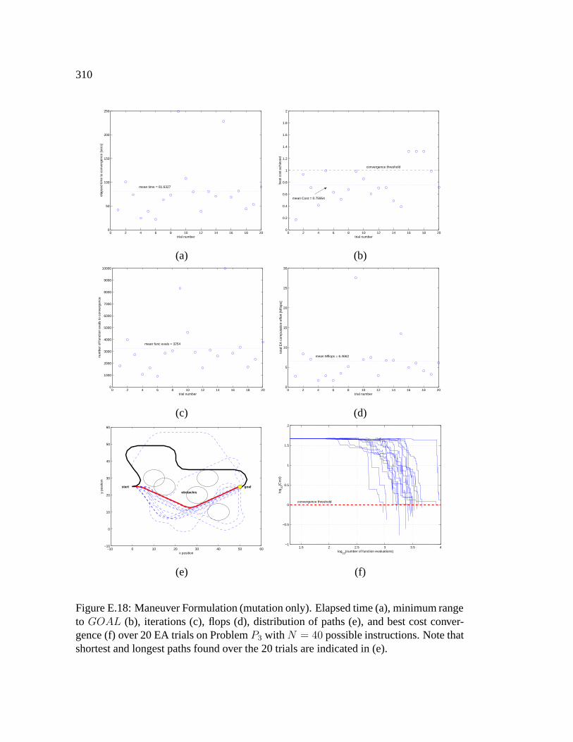
310

0 2 4 6 8 10 12 14 16 18 200

50

100

150

200

250

mean time = 81.6327

trial number

elap

sed

time

to c

onve

rgen

ce [s

ecs]

0 2 4 6 8 10 12 14 16 18 200

0.2

0.4

0.6

0.8

1

1.2

1.4

1.6

1.8

2

mean Cost = 0.75954

trial number

best

cos

t ach

ieve

d


(a) (b)

0 2 4 6 8 10 12 14 16 18 200

1000

2000

3000

4000

5000

6000

7000

8000

9000

10000


trial number

num

ber

of fu

nctio

n ev

als

to c

onve

rgen

ce

0 2 4 6 8 10 12 14 16 18 200

5

10

15

20

25

30


trial number

tota

l EA

com

puta

tion

effo

rt [M

flops

]

(c) (d)

−10 0 10 20 30 40 50 60−10

0

10

20

30

40

50

60

x position

y po

sitio

n

goalstart

obstacles

1.5 2 2.5 3 3.5 4−1

−0.5

0

0.5

1

1.5

2


log10


log 10

(Cos

t)

(e) (f)


311

0 2 4 6 8 10 12 14 16 18 200

50

100

150

200

250

300

mean time = 97.1101

trial number

elap

sed

time

to c

onve

rgen

ce [s

ecs]

0 2 4 6 8 10 12 14 16 18 200

0.2

0.4

0.6

0.8

1

1.2

1.4

1.6

1.8

2

mean Cost = 1.9643

trial number

best

cos

t ach

ieve

d


not shown: point at trial(3) = 27.23

(a) (b)

0 2 4 6 8 10 12 14 16 18 201000

2000

3000

4000

5000

6000

7000

8000

9000

10000


trial number

num

ber

of fu

nctio

n ev

als

to c

onve

rgen

ce

0 2 4 6 8 10 12 14 16 18 202

4

6

8

10

12

14

16

18

20


trial number

tota

l EA

com

puta

tion

effo

rt [M

flops

]

(c) (d)

−10 0 10 20 30 40 50 60−10

0

10

20

30

40

50

60

x position

y po

sitio

n

goalstart obstacles

1.5 2 2.5 3 3.5 4−1

−0.5

0

0.5

1

1.5

2


log10


log 10

(Cos

t)

(e) (f)


312

0 2 4 6 8 10 12 14 16 18 200

50

100

150

200

250

mean time = 107.885

trial number

elap

sed

time

to c

onve

rgen

ce [s

ecs]

0 2 4 6 8 10 12 14 16 18 200

0.2

0.4

0.6

0.8

1

1.2

1.4

1.6

1.8

2

mean Cost = 0.69946

trial number

best

cos

t ach

ieve

d


(a) (b)

0 2 4 6 8 10 12 14 16 18 200

1000

2000

3000

4000

5000

6000

7000

8000


trial number

num

ber

of fu

nctio

n ev

als

to c

onve

rgen

ce

0 2 4 6 8 10 12 14 16 18 200

5

10

15

20

25

30

35


trial number

tota

l EA

com

puta

tion

effo

rt [M

flops

]

(c) (d)

−10 0 10 20 30 40 50 60 70−10

0

10

20

30

40

50

60

70

x position

y po

sitio

n

goal

start obstacles

1.5 2 2.5 3 3.5 4−1

−0.5

0

0.5

1

1.5

2


log10


log 10

(Cos

t)

(e) (f)

Figure E.20: Maneuver (mutation only). Elapsed time (a), minimum range to GOAL(b), iterations (c), flops (d), distribution of paths (e), and best cost convergence (f) over20 EA trials on Problem P4. Note that shortest and longest paths found over the 20trials are indicated in (e). Mutation probabilities are ptime = 0.2 and pmaneuver = 0.4.

313

0 2 4 6 8 10 12 14 16 18 200

2

4

6

8

10

12

mean time = 3.3638

trial number

elap

sed

time

to c

onve

rgen

ce [s

ecs]

0 2 4 6 8 10 12 14 16 18 200

0.2

0.4

0.6

0.8

1

1.2

1.4

1.6

1.8

2

mean Cost = 0.66185

trial number

best

cos

t ach

ieve

d


(a) (b)

0 2 4 6 8 10 12 14 16 18 20100

200

300

400

500

600

700

800


trial number

num

ber

of fu

nctio

n ev

als

to c

onve

rgen

ce

0 2 4 6 8 10 12 14 16 18 200

0.1

0.2

0.3

0.4

0.5

0.6

0.7

0.8

0.9

1


trial number

tota

l EA

com

puta

tion

effo

rt [M

flops

]

(c) (d)

−10 0 10 20 30 40 50 60−10

0

10

20

30

40

50

60

x position

y po

sitio

n

goalstart

1.5 2 2.5 3 3.5 4−1

−0.5

0

0.5

1

1.5

2


log10


log 10

(Cos

t)

(e) (f)

Figure E.21: Maneuver Formulation (mutation + crossover). Elapsed time (a), mini-mum range to GOAL (b), iterations (c), flops (d), distribution of paths (e), and bestcost convergence (f) over 20 EA trials on Problem P1 with N = 40 possible instruc-tions. Note that shortest and longest paths found over the 20 trials are indicated in(e).

314

0 2 4 6 8 10 12 14 16 18 2010

15

20

25

30

35

40

45

50

55

60

mean time = 28.7769

trial number

elap

sed

time

to c

onve

rgen

ce [s

ecs]

0 2 4 6 8 10 12 14 16 18 200

0.2

0.4

0.6

0.8

1

1.2

1.4

1.6

1.8

2

mean Cost = 0.62605

trial number

best

cos

t ach

ieve

d


(a) (b)

0 2 4 6 8 10 12 14 16 18 20400

600

800

1000

1200

1400

1600

1800

2000

2200


trial number

num

ber

of fu

nctio

n ev

als

to c

onve

rgen

ce

0 2 4 6 8 10 12 14 16 18 200.5

1

1.5

2

2.5

3

3.5

4

4.5

5


trial number

tota

l EA

com

puta

tion

effo

rt [M

flops

]

(c) (d)

−10 0 10 20 30 40 50 60−10

0

10

20

30

40

50

60

x position

y po

sitio

n

goalstart

obstacles

1.5 2 2.5 3 3.5 4−1

−0.5

0

0.5

1

1.5

2


log10


log 10

(Cos

t)

(e) (f)


315

0 2 4 6 8 10 12 14 16 18 2020

40

60

80

100

120

140

mean time = 65.2111

trial number

elap

sed

time

to c

onve

rgen

ce [s

ecs]

0 2 4 6 8 10 12 14 16 18 200

0.2

0.4

0.6

0.8

1

1.2

1.4

1.6

1.8

2

mean Cost = 0.69064

trial number

best

cos

t ach

ieve

d


(a) (b)

0 2 4 6 8 10 12 14 16 18 20500

1000

1500

2000

2500

3000

3500

4000

4500

5000

5500


trial number

num

ber

of fu

nctio

n ev

als

to c

onve

rgen

ce

0 2 4 6 8 10 12 14 16 18 201

2

3

4

5

6

7

8

9

10

11


trial number

tota

l EA

com

puta

tion

effo

rt [M

flops

]

(c) (d)

−10 0 10 20 30 40 50 60−20

−10

0

10

20

30

40

50

60

x position

y po

sitio

n

goalstart

obstacles

1.5 2 2.5 3 3.5 4−0.5

0

0.5

1

1.5

2


log10


log 10

(Cos

t)

(e) (f)


316

0 2 4 6 8 10 12 14 16 18 2020

40

60

80

100

120

140

160

180

mean time = 66.926

trial number

elap

sed

time

to c

onve

rgen

ce [s

ecs]

0 2 4 6 8 10 12 14 16 18 200

0.2

0.4

0.6

0.8

1

1.2

1.4

1.6

1.8

2

mean Cost = 0.67059

trial number

best

cos

t ach

ieve

d


(a) (b)

0 2 4 6 8 10 12 14 16 18 200

1000

2000

3000

4000

5000

6000

7000


trial number

num

ber

of fu

nctio

n ev

als

to c

onve

rgen

ce

0 2 4 6 8 10 12 14 16 18 200

2

4

6

8

10

12

14


trial number

tota

l EA

com

puta

tion

effo

rt [M

flops

]

(c) (d)

−10 0 10 20 30 40 50 60

−10

0

10

20

30

40

50

60

x position

y po

sitio

n

goalstart obstacles

1.5 2 2.5 3 3.5 4−1

−0.5

0

0.5

1

1.5

2


log10


log 10

(Cos

t)

(e) (f)


317

0 2 4 6 8 10 12 14 16 18 200

50

100

150

200

250

300

350


trial number

elap

sed

time

to c

onve

rgen

ce [s

ecs]

0 2 4 6 8 10 12 14 16 18 200

0.2

0.4

0.6

0.8

1

1.2

1.4

1.6

1.8

2

mean Cost = 0.68119

trial number

best

cos

t ach

ieve

d


(a) (b)

0 2 4 6 8 10 12 14 16 18 200

1000

2000

3000

4000

5000

6000

7000

8000

9000

10000


trial number

num

ber

of fu

nctio

n ev

als

to c

onve

rgen

ce

0 2 4 6 8 10 12 14 16 18 200

5

10

15

20

25

30

35

40


trial number

tota

l EA

com

puta

tion

effo

rt [M

flops

]

(c) (d)

−30 −20 −10 0 10 20 30 40 50 60 70−30

−20

−10

0

10

20

30

40

50

60

70

x position

y po

sitio

n

goalstart obstacles

1.5 2 2.5 3 3.5 4−1

−0.5

0

0.5

1

1.5

2


log10


log 10

(Cos

t)

(e) (f)

Figure E.25: Maneuver (mutation + crossover). Elapsed time (a), minimum range toGOAL (b), iterations (c), flops (d), distribution of paths (e), and best cost convergence(f) over 20 EA trials on Problem P4. Note that shortest and longest paths found overthe 20 trials are indicated in (e). Note: ptime = 0.2 and pmaneuver = 0.4.

318

Appendix F

CONVERGENCE PROPERTIES OF EVOLUTIONARY

ALGORITHMS

This appendix serves as a brief summary of the major results detailed in Rudolph

[87] with regard to the convergence properties of EAs operating on both binary and

continuous variables.

F.1 A Binary Example

For genetic algorithms, in which states are coded in terms of binary strings (see Section

3.4.1), the states of the chain can be defined by every possible configuration of an entire

population of bit strings. Assuming bits are used in the coding and the size of the

population is µ, the number of possible states is given by 2µ. For example, with = 2

and µ = 1, the state space consists of four unique states:

Table F.1: Enumeration of the states of a binary population consisting of µ = 1 mem-bers of length = 2 bits each

1 2 3 4

(0,0) (0,1) (1,0) (1,1)

Recall that the probability transition matrix, P , which models the EA, represents the

combined effects of mutation and selection. For our purposes here, we ignore the ef-

fects of recombination (crossover). As we begin constructing the EA transition matrix,

we first consider a mutation matrix, M , whose entries, mij represent the probability

319

of mutating between two states i and j. We assume a mutation operator in the form

of equation (3.5), in which each of the bits in a string is flipped independently with

probability p. Thus, the probability of moving between any two states can be expressed

as:

PY (n) = y | X(n) = x = pH(x,y)(1− p)−H(x,y) (F.1)

where H(x, y) =∑

i=1 |xi − yi| is the Hamming distance (sum of bit differences)

between the two states x and y. Equation (F.1) expresses the fact that to move from

state x to y,H(x, y) bits need to be flipped while the number of bits while the remaining

−H(x, y) bits need to be unchanged. Computing each of these transition probabilities

for the 2-bit states in Table F.1 yields the matrix:

mij =

(1− p)2 p(1− p) p(1− p) p2

p(1− p) (1− p)2 p2 p(1− p)

p(1− p) p2 (1− p)2 p(1− p)

p2 p(1− p) p(1− p) (1− p)2

(F.2)

where, note that the probability of transitioning to the same state, pii reflects the fact

that each of the two bits must remain unchanged.

The effects of the selection operator must also be modeled in order to get the tran-

sition matrix for the entire evolutionary algorithm. We limit our attention to elitist

selection strategies which always preserve the best member of the population - a fea-

ture which will prove to be crucial for convergence to the global optimal solution. Thus,

we consider a selection operator of the form:

X(n+ 1) =

Y (n) if Y (n) ∈ G(X(n))

X(n) if Y (n) ∈ Gc(X(n))

(F.3)

Here, G(X(n)) is the gain set of X(n) given by those states satisfying G(x) = y ∈

S : f(y) < f(x) and Gc() is the set complement. In other words, we only allow

320

solutions Y (n) to survive if they are a member of a lower level set that the previous

best solution found - a state j is accepted only if it is better than state i. The matrix

entries corresponding to this selection operator can thus be described as:

• The probability that the Markov chain transitions to a state j that is better than

state i is just the probability to generate this state by mutation

• If state j is worse than state i, then it is not accepted and the probability of tran-

sitioning to such a state is zero

• The probability that the Markov chain stays in its current state is the sum over the

probabilities to generate a state by mutation that is not better than state i. Such

states are collected in the set Gc(i) = k ∈ S : f(k) ≥ f(i).

The entries of the overall transition matrix for this mutation and selection operators

can thus be summarized as:

pij =

mij if f(j) < f(i)∑k∈Gc(i)mik if j = i

0 if f(j) ≥ f(i)

(F.4)

where the mutation probabilities, mij , are those contained in the mutation matrix, M ,

given in equation (F.2). Note that these mutation probabilities are not problem specific.

Rather, they depend only on the mutation scheme chosen.

We can now apply this transition matrix to a particular problem. Consider the fol-

lowing objective function, which effectively tries to minimize the number of ”ones” in

the binary string:

f(x) =

if ‖x‖1 is odd

‖x‖1 if ‖x‖1 is even(F.5)

where ‖x‖1 =∑

i |xi| =∑

i xi. The behavior of this objective function for ‖X(0)‖ >

0 being odd is such that only a one-bit mutation can be improving. If, on the other

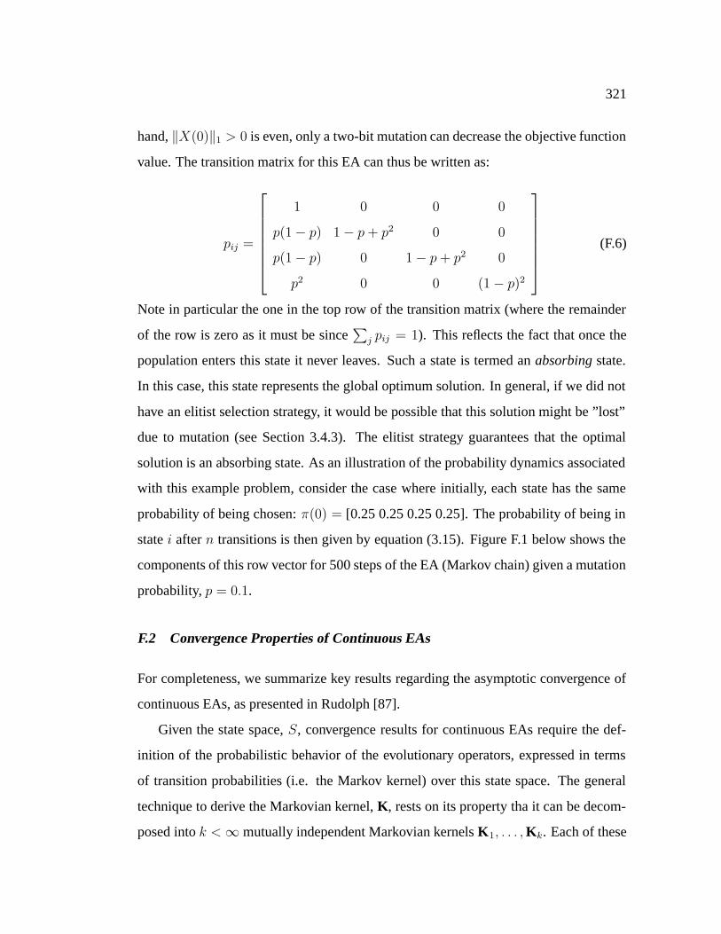
321

hand, ‖X(0)‖1 > 0 is even, only a two-bit mutation can decrease the objective function

value. The transition matrix for this EA can thus be written as:

pij =

1 0 0 0

p(1− p) 1− p+ p2 0 0

p(1− p) 0 1− p+ p2 0

p2 0 0 (1− p)2

(F.6)

Note in particular the one in the top row of the transition matrix (where the remainder

of the row is zero as it must be since∑

j pij = 1). This reflects the fact that once the

population enters this state it never leaves. Such a state is termed an absorbing state.

In this case, this state represents the global optimum solution. In general, if we did not

have an elitist selection strategy, it would be possible that this solution might be ”lost”

due to mutation (see Section 3.4.3). The elitist strategy guarantees that the optimal

solution is an absorbing state. As an illustration of the probability dynamics associated

with this example problem, consider the case where initially, each state has the same

probability of being chosen: π(0) = [0.25 0.25 0.25 0.25]. The probability of being in

state i after n transitions is then given by equation (3.15). Figure F.1 below shows the

components of this row vector for 500 steps of the EA (Markov chain) given a mutation

probability, p = 0.1.

F.2 Convergence Properties of Continuous EAs

For completeness, we summarize key results regarding the asymptotic convergence of

continuous EAs, as presented in Rudolph [87].

Given the state space, S, convergence results for continuous EAs require the def-

inition of the probabilistic behavior of the evolutionary operators, expressed in terms

of transition probabilities (i.e. the Markov kernel) over this state space. The general

technique to derive the Markovian kernel, K, rests on its property tha it can be decom-

posed into k <∞ mutually independent Markovian kernels K1, . . . ,Kk. Each of these

322

0 50 100 150 200 250 300 350 400 450 5000

0.1

0.2

0.3

0.4

0.5

0.6

0.7

0.8

0.9

1

number of steps

Pro

babi

lity

to b

e in

sta

te i

P(state 1)

P(state 4)

P(state 2,3)

Figure F.1: Illustration of the EA probability dynamics for each of the possible statesof the simple 2-bit population starting from a uniform initial probability distribution ofπ(0) = [0.25 0.25 0.25 0.25].

323

describe a single evolutionary operator, and the aggregate Markovian kernel, K is their

product kernel:

K(x,A) = (K1,K2 · · ·Kk) (x,A)

=

∫S

K1(x1, dx2)

∫S

K2(x2, dx3) · · ·

· · ·∫S

Kk−2(xk−2dxk−1)

∫S

Kk−1(xk−1, dxk)Kk(xk, A)

Rudolph [87] has developed an expression for this Markovian kernel for an evolutionary

algorithm restricted to the set Aε, where Aε = x ∈ S : b(x) ≤ f : ∗ + ε denotes the

set of solutions x whose best value, b(x), falls within ε of the optimal solution.

The properties of this kernel required for convergence to a global optimum can be

stated, namely:

Theorem 2 ([87], p201) A population-based evolutionary algorithm, whose Marko-

vian kernel satisfies the conditions K(x,Aε) ≥ δ > 0 for all x ∈ Acε = S \ Aε and

K(x,Aε) = 1 for x ∈ Aε will converge completely to the global minimum of a real-

valued function f regardless of the initial distribution.

In particular, we can denote the Markovian kernel, K as the product of the stochas-

tic kernels corresponding to crossover, mutation, and selection. It can be shown [87]

that a sufficient condition for an EA to satisfy the preconditions of Theorem 2 is that

Kcms(x,Aε) ≥ δ > 0 for x ∈ Aε.

Theorem 3 ([87], p201) Let X0 ∈ S be the initial population of some elitist EA and

let Kc,Km,Ks denote the stochastic kernels of the crossover, mutation, and selection

operator, respectively. If the conditions:

1. ∃δc > 0 : ∀x ∈ S : Kc(x,B(x)) ≥ δc

2. ∃δm > 0 : ∀x ∈ B(X0) : Km(x,Aε) ≥ δm

324

3. ∃δs > 0 : ∀x ∈ S : Ks(x,B(x)) ≥ δs

hold simultaneously, the for every ε > 0 there exists a δ > 0 such that Kcms(x,Aε) ≥

δ > 0 for every x ∈ B(X0).

The proof of Theorem 3 relies on several properties. One of these involves the

mutation distribution.

Definition 1 Let z be a random vector with support R and D = diag(d1, d2, . . . , d)

be a diagonal matrix with det(D) = 1 and di ≥ dmin > 0. A mutation distribution,

Fz will be termed strictly covering if z can be generated via z = σTDz for arbitrary

orthogonal matrix T and where σ is allowed to vary in a closed and bounded subset of

σ ∈ R : σ > 0.

With this definition, one can summarize the conditions for global convergence for

population-based continuous EAs:

Theorem 4 ([87],p.205) A population-based EA with elitism that uses

1. multipoint, parameterized uniform, parameterized immediate, gene pool, or pa-

rameterized intermediate gene pool recombination (with replacement)

2. a strictly covering mutation distribution,

3. standard proportional, q-fold binary tournament, or top µ selection

converges completely to the global minimum of an objective function f : R →R from

the set f ∈ F : f(x)→∞ as ‖x‖ → ∞.

325

Vita

Brian Capozzi received the B.S. degree in Aerospace and Mechanical Engineering from

the University of Notre Dame in 1994 and a Master’s degree in Aeronautics and Astro-

nautics from the University of Washington in 1996. Upon completion of his Master’s

degree, Brian spent two years working for Stirling Dynamics on the development of

active force-feedback control devices, including cyclic and collective levers for heli-

copters as well as an active throttle for fixed-wing aircraft. In late 1998, he began work-

ing in the area of path planning for autonomous vehicles, for which he subsequently

received a Ph.D. in Aeronautics and Astronautics from the University of Washington in

2001.

evolution-basedpath planning and management for autonomous

Documents