EXACT STUDIES OF EQUILIBRIUM AND

NONEQUILIBRIUM PROPERTIES OF CORRELATED

BOSONS IN ONE-DIMENSIONAL LATTICES

A Dissertation

submitted to the Faculty of the

Graduate School of Arts and Sciences

of Georgetown University

in partial fulfillment of the requirements for the

degree of

Doctor of Philosophy

in Physics

By

Kai He, M.S.

Washington, DC

July 2013

EXACT STUDIES OF EQUILIBRIUM AND

NONEQUILIBRIUM PROPERTIES OF CORRELATED

BOSONS IN ONE-DIMENSIONAL LATTICES

Kai He, M.S.

Advisor: Marcos Rigol, Ph.D.

Abstract

In this thesis, we study both equilibrium and nonequilibrium properties of

hard-core bosons trapped in one-dimensional lattices. To perform many-

body analyses of large systems, we utilize exact numerical approaches in-

cluding an approach based on the Bose-Fermi mapping and the Lanczos

method. We study noise correlations of hard-core bosons in homogeneous

lattices, period-two superlattices, and disordered lattices, and focus on the

scaling of such correlations with system size in the superfluid and insulat-

ing phases. We find that superfluid phases exhibit a leading linear scaling,

while the leading terms in the scaling of the Mott-insulting and Bose-glass

phases are constants. We also characterize the disorder-induced phase tran-

sition between a superfluid and a Bose-glass phase in an incommensurate

lattice system by determining the critical exponents in the scaling of the

momentum distribution and the noise correlations. We show that the phase

transition is signaled by peaks in the first derivatives of the noise correla-

tions with respect to the strength of quasiperiodic disorder, and the height

of the peaks diverges with increasing system size. Furthermore, related to

the nonequilibrium properties of isolated systems, we investigate the initial-

state dependence of the outcome of relaxation dynamics following quantum

quenches. Starting from a thermal state associated with a finite initial

temperature, the entropy of the generalized Gibbs ensemble, introduced to

describe integrable systems after relaxation, is found to be generally differ-

ent from the entropy in thermal equilibrium. The disagreement is explained

to stem from the distinction between the conserved quantities in the initial

state and those in the thermal ensembles. On the other hand, if the initial

state is selected to be an eigenstate of a nonintegrable (chaotic) model, a

ii

thermal-like “ergodic” sampling of the eigenstates of the integrable Hamil-

tonian is unveiled by computing the weighted energy density. We show

that the distribution of the conserved quantities in the chaotic initial state

coincides with the thermal ones in thermodynamic limit. Our results in-

dicate that quenches starting from nonintegrable initial states will lead to

thermalization even if the final system is integrable.

iii

Acknowledgements

I am very thankful to Georgetown University for providing me the oppor-

tunity to pursue my PhD studies and conduct researches with both educa-

tional and financial support. I thank all the faculty and staff members who

helped me directly or indirectly during my stay at the university. I also

thank Pennsylvania State University for support during my visit there.

I have my deepest gratitude towards my advisor, Prof. Marcos Rigol, for

the invaluable scientific guidance and advices, for the positive criticism, for

the constant encouragement, for the massive supports and helps that are

not only research-related but also on life. Without his mentoring this thesis

would not have been possible.

I would like to thank Dr. Charles Clark for hosting my visit at NIST and

being a member of my dissertation committee. I also thank Dr. Indubala

Satija for her direction and helps, and Dr. Ana Maria Rey for the important

contribution to the project during our collaboration at NIST.

I thank Prof. Jim Freericks, Prof. Jeffery Urbach, and Dr. Predrag Nikolic

for their useful feedbacks on my thesis as the dissertation committee mem-

bers.

I would like to thank Itay Hen, Christopher Varney, and Ehsan Khatami

for offering me a lot of helps and suggestions, especially at the beginning

of my researches. They generously shared with me their knowledge and

experiences in performing computational simulations and developing highly

parallel programs. I am highly grateful to Juan Carrasquilla, who constantly

showed his patience and helpfulness whenever asked a question. I benefited

tremendously from meaningful and enlightening discussions with him, in

both physics and technical areas.

iv

I show all my thankfulness to my past and current groupmates, who created

an exceptional working atmosphere with extremely joyful dynamics. They

are Rubem Mondaini, Andrea Di Ciolo, Baoming Tang, Christian Gramsch,

Andrew Jreissaty, and Jennifer Brown, in addition to Itay, Chris, Ehsan,

and Juan.

Many thanks go to my friends and colleagues in the department of physics

in Georgetown University. To Yizhi Ge, Wen Shen for academic and career

suggestions. To Karlis Mikelsons, Herbert Fotso, among others, for pleasant

and insightful conversations within and beyond science. To Kristin Lucas,

Pramukta Kumar, Yayue Xiao, John Harrison, and more, for helping me

during my completion of graduate courses and making difficult studies more

joyful.

Finally, I can never be too grateful to my family. My parents, though

distantly apart from me, gave me endless emotional support and courage to

finish my education. To my wife, Yinyue Hu, thank you for your love, your

care, your consideration, for all you have done for me.

v

Contents

1 Introduction . . . . . . . . . . . . . . . . . . . . . . . . . . . . . . . . . . . . . 1

1.1 Optical Lattices . . . . . . . . . . . . . . . . . . . . . . . . . . . . . . . . 2

1.2 Ground-band Bloch States and Wannier Functions . . . . . . . . . . . . 4

1.3 Bose-Hubbard Model and Superfluid-Mott Insulator Transition . . . . . 5

1.4 Tonks-Girardeau Gas in 1D . . . . . . . . . . . . . . . . . . . . . . . . . 8

1.5 Overview . . . . . . . . . . . . . . . . . . . . . . . . . . . . . . . . . . . 10

2 Models and Exact Approach . . . . . . . . . . . . . . . . . . . . . . . . . . . . 13

2.1 Hard-core Bosons and Bose-Fermi Mapping . . . . . . . . . . . . . . . . 13

2.2 Slater Determinants and Correlation Functions . . . . . . . . . . . . . . 15

2.2.1 One-Particle Correlations . . . . . . . . . . . . . . . . . . . . . . 15

2.2.2 Noise Correlations . . . . . . . . . . . . . . . . . . . . . . . . . . 17

3 Noise Correlations of Hard-core Bosons in 1D Lattices . . . . . . . . . . . . . 19

3.1 Time-of-flight Measurements and Noise Correlations . . . . . . . . . . . 19

3.2 Homogeneous System . . . . . . . . . . . . . . . . . . . . . . . . . . . . 22

3.3 Period-two Superlattice . . . . . . . . . . . . . . . . . . . . . . . . . . . 25

3.4 Disordered Lattice . . . . . . . . . . . . . . . . . . . . . . . . . . . . . . 29

4 Quantum Phase Transition in Incommensurate Lattices . . . . . . . . . . . . 34

4.1 Quasiperiodic Systems and Disorder-induced Phase Transition . . . . . 35

4.1.1 Incommensurate Lattice . . . . . . . . . . . . . . . . . . . . . . . 36

4.1.2 Localization-delocalization Transition . . . . . . . . . . . . . . . 36

4.2 Quantum Correlations: Scaling Analysis . . . . . . . . . . . . . . . . . . 37

4.3 Quantum Phase Transition . . . . . . . . . . . . . . . . . . . . . . . . . 41

4.4 Absence of Primary Sublattice Peaks . . . . . . . . . . . . . . . . . . . . 44

vi

5 General Considerations on Quantum Quenches . . . . . . . . . . . . . . . . . 47

5.1 Relaxation in Integrable Systems . . . . . . . . . . . . . . . . . . . . . . 47

5.1.1 Diagonal Ensemble: State after Relaxation . . . . . . . . . . . . 48

5.1.1.1 Pure Initial State . . . . . . . . . . . . . . . . . . . . . 48

5.1.1.2 Thermal Initial State . . . . . . . . . . . . . . . . . . . 49

5.1.2 Canonical and Grand-canonical Ensemble . . . . . . . . . . . . . 50

5.1.3 Generalized Gibbs Ensemble . . . . . . . . . . . . . . . . . . . . 51

5.2 Entropies and Observables . . . . . . . . . . . . . . . . . . . . . . . . . . 52

5.3 Thermalization in isolated systems . . . . . . . . . . . . . . . . . . . . . 53

6 Quench Dynamics of Thermal Initial States in Integrable Systems . . . . . . 57

6.1 Initial-State Dependence . . . . . . . . . . . . . . . . . . . . . . . . . . . 57

6.2 Model Hamiltonian and Quench Protocol . . . . . . . . . . . . . . . . . 59

6.3 Weights in the Ensembles . . . . . . . . . . . . . . . . . . . . . . . . . . 59

6.4 Entropies . . . . . . . . . . . . . . . . . . . . . . . . . . . . . . . . . . . 63

6.5 Conserved Quantities . . . . . . . . . . . . . . . . . . . . . . . . . . . . . 67

7 Quench Dynamics of Chaotic Initial States in Integrable Systems . . . . . . . 73

7.1 Motivation . . . . . . . . . . . . . . . . . . . . . . . . . . . . . . . . . . 74

7.2 Model Hamiltonian and Quench Protocol . . . . . . . . . . . . . . . . . 75

7.3 Overlaps . . . . . . . . . . . . . . . . . . . . . . . . . . . . . . . . . . . . 76

7.4 Entropies . . . . . . . . . . . . . . . . . . . . . . . . . . . . . . . . . . . 82

7.5 Conserved Quantities . . . . . . . . . . . . . . . . . . . . . . . . . . . . . 85

7.6 Momentum Distribution Functions . . . . . . . . . . . . . . . . . . . . . 88

8 Summary and Conclusions . . . . . . . . . . . . . . . . . . . . . . . . . . . . . 90

Bibliography . . . . . . . . . . . . . . . . . . . . . . . . . . . . . . . . . . . . . . 94

vii

List of Figures

1.1 Optical lattice . . . . . . . . . . . . . . . . . . . . . . . . . . . . . . . . . 3

1.2 Bloch band structure . . . . . . . . . . . . . . . . . . . . . . . . . . . . . 5

1.3 Superfluid and Mott insulator . . . . . . . . . . . . . . . . . . . . . . . . 6

1.4 Superfluid-Mott insulator transition in 3D lattices . . . . . . . . . . . . 8

1.5 Quasi-1D tubes . . . . . . . . . . . . . . . . . . . . . . . . . . . . . . . . 9

3.1 Time-of-flight imaging of expanding atom clouds . . . . . . . . . . . . . 20

3.2 Single-shot absorption image and noise correlations of a Mott insulator . 21

3.3 Noise correlations in a homogeneous lattice . . . . . . . . . . . . . . . . 23

3.4 Noise correlations as a function of k and ρ . . . . . . . . . . . . . . . . . 24

3.5 Scaling of noise correlations in homogeneous systems . . . . . . . . . . . 25

3.6 Noise correlations for the Mott phase in a half-filled superlattice . . . . 26

3.7 Noise correlations as a function of k and ρ in a half-filled superlattice . . 27

3.8 Sublattice peak ∆πa,0 as a function of the filling factor . . . . . . . . . . 27

3.9 Scaling of Noise correlations for the fractional Mott phase . . . . . . . . 28

3.10 Off-diagonal one-particle correlations in disordered systems . . . . . . . 30

3.11 Noise correlations in disordered lattices . . . . . . . . . . . . . . . . . . 31

3.12 Comparison in the noise correlations between the superfluid, fractional

Mott, and Bose-glass phases . . . . . . . . . . . . . . . . . . . . . . . . . 31

3.13 Scaling of the noise correlations in disordered systems . . . . . . . . . . 32

3.14 Noise correlation peak as a function of disorder . . . . . . . . . . . . . . 33

4.1 Momentum distribution and noise correlations in quasiperiodic lattices . 38

4.2 Scaling of nk=0 and ∆00 for various disorder strength . . . . . . . . . . . 39

4.3 Absence of scaling in the sublattice peak . . . . . . . . . . . . . . . . . . 40

4.4 Noise correlations at an incommensurate filling . . . . . . . . . . . . . . 41

4.5 Superfluid–Bose glass transition as a function of disorder . . . . . . . . . 42

viii

4.6 Anderson transition in free fermions . . . . . . . . . . . . . . . . . . . . 43

4.7 Bosons vs. fermions at the transition point . . . . . . . . . . . . . . . . 44

4.8 Absence of sublattice peaks in the momentum distributions . . . . . . . 45

4.9 Missing peaks in period-4 and period-8 superlattices . . . . . . . . . . . 46

5.1 Eigenstate Thermalization Hypothesis . . . . . . . . . . . . . . . . . . . 54

5.2 Generalized Eigenstate Thermalization Hypothesis . . . . . . . . . . . . 56

6.1 Weights in the DE and the CE. I . . . . . . . . . . . . . . . . . . . . . . 60

6.2 Weights in the DE and the CE. II . . . . . . . . . . . . . . . . . . . . . 61

6.3 Weighted energy densities . . . . . . . . . . . . . . . . . . . . . . . . . . 62

6.4 Entropy per site vs. system size . . . . . . . . . . . . . . . . . . . . . . . 64

6.5 Entropy difference between the GGE and the GE . . . . . . . . . . . . . 65

6.6 (SGE − SGGE)/L as a function of AI(AF ) at fixed temperatures . . . . . 66

6.7 (SGE − SGGE)/L as a function of T for fixed quenches . . . . . . . . . . 67

6.8 Distribution of conserved quantities . . . . . . . . . . . . . . . . . . . . 68

6.9 Scaling of Integrated difference ∆I . . . . . . . . . . . . . . . . . . . . . 69

6.10 ∆I vs. strength of the quench . . . . . . . . . . . . . . . . . . . . . . . . 70

6.11 ∆I vs. initial temperature . . . . . . . . . . . . . . . . . . . . . . . . . . 71

7.1 Coarse-grained plot of weights in the DE and the CE . . . . . . . . . . . 77

7.2 Weighted density functions P (E) for quenches type I and type II . . . . 79

7.3 Another type of weighted energy density P (ǫ) . . . . . . . . . . . . . . . 81

7.4 Entropy per site for various ensembles . . . . . . . . . . . . . . . . . . . 83

7.5 (SGE − SDE)/L vs. quench strength for both types of quenches . . . . . 84

7.6 Conserved quantities in the initial state and the GE . . . . . . . . . . . 86

7.7 Integrated difference ∆I as a function of the quench strength . . . . . . 87

7.8 Momentum distributions in the DE, the GGE, and the GE . . . . . . . 88

7.9 ∆mDE as a function of the quench strength . . . . . . . . . . . . . . . . 89

ix

List of Tables

3.1 Fitting parameters for the homogeneous case. . . . . . . . . . . . . . . . 24

3.2 Fitting parameters for the superlattice case. . . . . . . . . . . . . . . . . 29

x

1

Introduction

The experimental realization of a Bose-Einstein condensate (BEC) at the National In-

stitute of Standards and Technology, Boulder in 1995 [1] was an unprecedented moment

in the field of atomic and molecular physics and a rewarding moment for decades of

intensive efforts, both theoretical and experimental, since the remarkable prediction

made by Albert Einstein 70 years before. His theory predicted that a noninteracting

gas of bosonic atoms, if cooled below some very low temperature, should collapse into a

macroscopic coherent state in which the majority of atoms occupied the lowest energy

eigenstate of the noninteracting Hamiltonian.

The success in attaining BEC was attributed to the magnificent advance in the

cooling techniques that made the access to a nano-kelvin temperature possible. The

cooling of atoms was accomplished in a two-step process, which started with laser

cooling and further continued with radio-frequency (RF) evaporative cooling [1]. In

the first stage, the dilute vapor of alkali atoms was trapped in a magneto-optic trap

created by intersecting six orthogonal laser beams, in which the motion of atoms was

slowed down due to the absorption of photons. Because of the Doppler shift, one was

able to precisely red-detune the laser frequency to pick out the “fast” atoms in all six

directions and only slow them down without affecting any of the rest of the particles

that traveled at other velocities. The laser cooling technique was able to pre-cool the

species to a temperature of microkelvins, but not any further owing to the recoil energy

of the spontaneous emission. At this point the evaporative cooling was performed. The

sample was loaded into a strong magnetic trap where the higher energy atoms were

selectively released with the use of RF magnetic fields; the remaining atoms then re-

1

thermalized to a colder temperature. In this way a temperature of the order of 100nK

was reached and the BEC began to form [1].

Bose-Einstein condensation opened up a window to the studies of ultracold degen-

erate gases by enabling scientists to control the degrees of freedom at the atomic level.

Meanwhile, BECs have become an attractive testing ground for interacting many-body

physics. Even though a condensate is essentially an extremely dilute gas of bosons

characterized by weak interactions, the presence of the interactions makes BEC differ-

ent from a cloud of coherent photons and become a valuable host of rich many-body

phenomena, such as high-temperature superconductivity and vortices, amongst others.

The superfluid behavior of BEC was revealed by the observation of critical velocities in

experiments where the condensate was stirred by a laser beam [2, 3], or dragged through

an optical lattice by a displaced magnetic trapping potential [4, 5]. Quantized vortices

were also experimentally created by various means, such as manipulating the phase pat-

tern of a two-component condensate via an interference technique [6], spinning BEC

samples with a laser [7, 8], and cooling a rotating normal gas below the condensation

temperature [9]. Theoretically, the understanding of such quantum phenomena as well

as other interesting physics of BEC was first gained through the Gross-Pitaevskii (GP)

equation, in the spirit of the mean field theory, and it was further improved by the

Bogoliubov theory, which gives a correction to the GP equation due to small quantum

fluctuations. These theories have been very successful by describing BECs in a picture

of weakly interacting quasiparticles.

1.1 Optical Lattices

The desire of scientists to enter the strongly correlated regime of ultracold atoms has in-

creased with the years, because strong interactions play a critical role in the emergence

of important many-body phenomena. One of the technical development that finally

bridged BEC and condensed matter physics was the introduction of optical lattices.

This technique aims to trap ultracold atoms in periodic standing light patterns gen-

erated by interfering laser beams (Fig. 1.1). In the presence of the light field, electric

dipole moments in the atoms are induced due to a AC Stark shift, which in turn give

rise to a dipole force upon the atoms [11]

Fdip(r) =1

2α(ωL)∇|E(r)|2, (1.1)

2

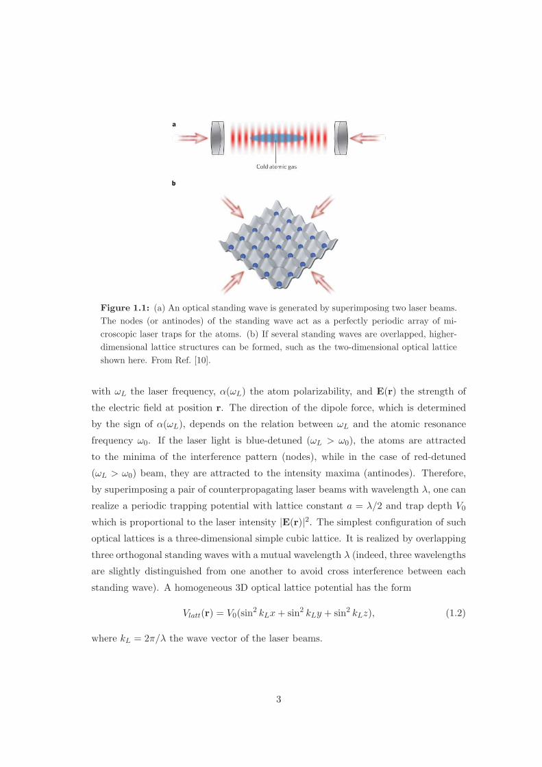
Figure 1.1: (a) An optical standing wave is generated by superimposing two laser beams.

The nodes (or antinodes) of the standing wave act as a perfectly periodic array of mi-

croscopic laser traps for the atoms. (b) If several standing waves are overlapped, higher-

dimensional lattice structures can be formed, such as the two-dimensional optical lattice

shown here. From Ref. [10].

with ωL the laser frequency, α(ωL) the atom polarizability, and E(r) the strength of

the electric field at position r. The direction of the dipole force, which is determined

by the sign of α(ωL), depends on the relation between ωL and the atomic resonance

frequency ω0. If the laser light is blue-detuned (ωL > ω0), the atoms are attracted

to the minima of the interference pattern (nodes), while in the case of red-detuned

(ωL > ω0) beam, they are attracted to the intensity maxima (antinodes). Therefore,

by superimposing a pair of counterpropagating laser beams with wavelength λ, one can

realize a periodic trapping potential with lattice constant a = λ/2 and trap depth V0

which is proportional to the laser intensity |E(r)|2. The simplest configuration of such

optical lattices is a three-dimensional simple cubic lattice. It is realized by overlapping

three orthogonal standing waves with a mutual wavelength λ (indeed, three wavelengths

are slightly distinguished from one another to avoid cross interference between each

standing wave). A homogeneous 3D optical lattice potential has the form

Vlatt(r) = V0(sin2 kLx+ sin2 kLy + sin2 kLz), (1.2)

where kL = 2π/λ the wave vector of the laser beams.

3

Usually the lattice potential V0 is very strong so that each trap can be approximated

by a harmonic-oscillator potential with characteristic energy ~ω about 10 times the

recoil energy of the laser Er = ~2k2L/2m. With such a tight-confining optical lattice

one is able to reduce the kinetic energy of ultracold atoms to only the tunneling and

thus the interparticle interaction becomes a comparable energy scale. As a consequence,

the interplay between the kinetic energy and the interaction energy is emphasized in

lattices.

1.2 Ground-band Bloch States and Wannier Functions

The generic system of bosonic atoms in an optical lattice is described by the Hamilto-

nian

H =

∫

dr ψ†(r)

[

p

2m+ Vlatt(r) + Vext(r)

]

ψ(r)

+1

2

∫∫

drdr′ψ†(r)ψ†(r′)U(r− r′)ψ(r′)ψ(r), (1.3)

where ψ(r)[ψ†(r)] is the bosonic field operator for destroying(creating) an atom at po-

sition r, Vlatt(r) and Vext(r) describe the optical lattice potential (with amplitude V0)

and an external potential, respectively, and U(r − r′) denotes the interparticle inter-

action. Now, if we neglect the additional on-site potential [Vext(r) = 0] and consider

the single-particle solution of the Hamiltonian, the exact eigenstates are Bloch states

due to the periodic nature of the lattice potential. Note that, in the assumption of

strong optical confinement V0 ≫ Er, each trap contains harmonic vibrational levels

separated by ~ω. The Bloch state band structure is shown in Fig. 1.2, where one can

see that the energy gap between the ground band and the second lowest band ap-

proaches the level spacing ~ω as the lattice depth V0/Er increases. Therefore, for low

temperatures of interest (T ≪ ~ω), atoms are considered locked in the lowest vibra-

tional level and the single-particle wavefunctions are ground-band Bloch states ψk(r)

with quasi-momentum k.

On the other hand, a tight binding description of the sufficiently deep lattice allows

one to express the Bloch states in terms of a set of exponentially localized Wannier

functions wj(r) by a Fourier transform

ψk(r) =∑

j

wj(r)eikRj , (1.4)

4

Figure 1.2: Band structure of the Bloch states for different lattice depths V0/Er = 20,

10, and 0, respectively. In a deep lattice, the ground band approaches a flat one and the

width of the first band gap is approximately ~ω. From Ref. [12].

with Rj the lattice vector of site j. To a very good approximation, these Wannier

functions are selected as the ground states of local harmonic oscillators at each lattice

site, and such a set of Wannier functions forms a complete basis. Therefore, the bosonic

field operators can be written as

ψ(r) =∑

j

bj wj(r), ψ†(r) =∑

j

b†j w∗j (r). (1.5)

Here bj(b†j) is the annihilation(creation) operator for bosons in the Wannier state wj(r)

and they obey the commutation relations

[bi, b†j ] = δij , [bi, bj ] = [b†i , b

†j ] = 0. (1.6)

1.3 Bose-Hubbard Model and Superfluid-Mott Insulator

Transition

The localized nature of the selected Wannier functions justifies the following approxi-

mations. Up to a constant shift (the ground-state vibrational energy) in the chemical

potential, the kinetic energy of the lattice bosons is essentially frozen except for the

hopping restricted between nearest neighbors. The strength of the interaction energy,

which is related to the overlapping of Wannier states, is only non-negligible for atoms

on the same site because of the localization of the Gaussian shaped harmonic oscillator

5

Figure 1.3: Illustration of the superlattice phase (top) and the Mott-insulating phase

(bottom) of a Bose gas in an optical lattice.

wavefunction. As a result, The Hamiltonian (1.3) can be written as

HBH = −t∑

NN

(

b†i bj +H.c.)

+∑

i

Vi ni +U

2

∑

i

ni(ni − 1), (1.7)

where NN indicates that the sum runs over pairs of (i, j) that correspond to nearest

neighbors and ni = b†i bi the site occupation operator. This is the very well-known

Bose-Hubbard model. Here, t and U denote the nearest-neighbor hopping parameter

and the strength of the on-site repulsion, respectively,

t =

∫

dr w∗i (r)

[

p

2m+ Vlatt(r)

]

wj(r),

U =

∫

dr U(0)|wi(r)|4, (1.8)

and Vi describes the external potential imposed on top of the underlying lattice.

The Bose-Hubbard model reflects, through the ratio of U to t, the competition

between the tendency of atoms to delocalize over the whole lattice (kinetic energy) and

the resistance of multiple occupancy at a single site (interaction energy). As a result,

two important quantum phases are present in the ground state of the homogeneous

Bose-Hubbard model, as depicted in Fig. 1.3.

In the regime of weak interaction U/t ≪ 1 the system exhibits a coherent phase,

which is referred to as the superfluid phase, characterized by long-range order. In the

noninteracting limit U = 0, this is trivially an ideal BEC with all atoms occupying the

6

zero-momentum Bloch state in the ground band. The many-body ground state in a

lattice with N atoms in L sites can be written as

|ΨBEC〉 =1√N !

(

1√L

L∑

i

b†i

)N

|0〉. (1.9)

As a result of the clear definition in momentum space, the perfect superfluid favors the

wavefunction to be completely extended over the entire lattice and therefore can be

described as a single coherent matter wave.

On the other hand, a Mott-insulating phase emerges in the strong-coupling limit

U/t ≫ 1 when each site is exactly occupied by an integer number of atoms. Because

of the dominance of repulsive interaction, the integer-filled system precludes hopping

between sites and all atoms are nailed at single lattice sites resulting in an absence of

density fluctuation (Fig. 1.3). The ground state of a Mott insulator is given by

|ΨMott〉 =1√n!

L∏

i

(

b†i

)n|0〉, (1.10)

with n = N/L(= 1, 2, · · · ) the local occupation number. It is a product of Fock states

with precisely n atoms per site and the phase coherence is missing across lattice sites.

Moreover, the Mott insulating phase is incompressible due to the particle-hole excitation

gaps in the many-body energy spectrum.

In between the two limits, a quantum phase transition from the superfluid phase

to the Mott-insulating phase as a function of U/t is expected to happen in the Bose-

Hubbard model. Following the theoretical proposal made by Jaksch et al. [14], the

superfluid to Mott insulator transition was experimentally observed in a 3D optical

lattice [13]. In the experiment, a BEC was loaded onto a simple cubic lattice super-

imposed by a harmonic trap. By gradually tuning up the depth of the lattice V0/Er,

U/t monotonically increased across a critical transition value, at which a Mott insu-

lator began to form in the center of the trap. The disappearance of phase coherence

was observed through a time-of-flight measurement, as shown in Fig. 1.4. Later, the

superfluid-Mott insulator transition was also realized in 2D [15] and 1D optical lattices

[16, 17] as well.

7

Figure 1.4: Absorption images of multiple matter wave interference patterns. These were

obtained after suddenly releasing the atoms from an optical lattice with a depth of (a)

0Er, (b) 3Er, (c) 7Er, (d) 10Er, (e) 13Er, (f) 14Er, (g) 16Er, and (h) 20Er, after a time

of flight of 15 ms. Er is the recoil energy. A clear suggestion of the transition is provided,

as the sharp interference peaks that characterize the superfluid phase disappear for large

values of the lattice depth. From Ref. [13].

1.4 Tonks-Girardeau Gas in 1D

Another opportunity offered by introducing optical lattices is accessing reduced dimen-

sionalities, which has triggered even more remarkable explorations towards the strongly

correlated regime [18]. A quasi-1D geometry can be created through a 2D optical lattice

potential. As illustrated in Fig. 1.5, an array of quasi-1D tubes along the longitudinal

direction is constructed by only overlapping a pair of optical standing waves in the

two orthogonal transverse directions. As a result, the atoms are tightly confined in the

tubes where motion in the other two dimensions is prohibited. Additionally, if a weaker

periodic potential is independently applied along the longitudinal axis, one can form a

1D lattice system. For bosons, this can be described by the 1D Bose-Hubbard model.

Both 1D gases, in the continuum [19] and in a lattice [20–22], have been realized.

Compared to 3D, 1D systems fascinate physicists with their mathematical beauty,

counter-intuitive properties, and the emergence of phenomena that does not occur in

higher dimensions [18]. For example, in 1D the role of interaction is most dominant

in the limit of low density, in contrast to the opposite but more intuitive limit in

3D [12]. Also, Bose-Einstein condensation is known not to occur in 1D interacting

bosonic systems [18]. On top of various interesting aspects of 1D many-body physics,

their exact solvability in many cases is what emphasizes their significance. For lattice

bosons, the 1D Bose-Hubbard model has an exact solution in the limit U/t→ ∞. Such a

8

Figure 1.5: (a) Two- and (b) three-dimensional optical lattice potential formed by su-

perimposing two or three orthogonal standing waves. From Ref. [23].

model describes a gas of impenetrable particles known as hard-core bosons (HCBs), the

concept of which was first introduced by Girardeau [24]. Thus they are also referred to

as Tonks-Girardeau bosons. Girardeau provided an exact one-to-one mapping between

these strongly-correlated bosons and the spinless noninteracting fermions in 1D, and

the local and thermodynamic properties of HCBs can be easily computed through the

correspondence to the Fermi counterparts. In 1D, the Bose-Hubbard model in the

hard-core regime reduces to

HHCB = −t∑

i

(

b†i bi+1 +H.c.)

+∑

i

Vi ni, (1.11)

with a constraint b†2i = b2i = 0 that forbids double occupancy of the same site. Such

a Hamiltonian can be mapped onto the XY spin-1/2 model [25] and further onto

a noninteracting fermion lattice model (for details see Chapter 2). Although these

fermionized bosons behave locally very much like noninteracting fermions, they are

intrinsically distinct in the quantum statistics which is reflected in momentum space.

Moreover, HCBs in 1D have other interesting properties. For example, despite of

the absence of true condensation, they exhibit quasicondensation at zero temperature

9

reflected by power-law decaying off-diagonal correlations (quasi-long range order) [26–

29].

It was pointed out that the Tonks-Girardeau gas corresponded to a certain regime

of large positive scattering length, low densities and low temperatures and as such it

could be realized in experiments [30–32]. In 2004, utilizing a deep 2D optical lattice

in the presence of a weak dipole force trap along the tubes, Kinoshita et al. managed

to prepare a 1D HCB gas by precisely tightening the transverse periodic confinement

to reach the required scattering length [19]. In the same year, Paredes et al. reported

another success on the access to the strongly-interacting regime based on the 1D Bose-

Hubbard model [22]. In this case, a gas of ultracold bosonic atoms was loaded onto

a 1D lattice which, as already described, was formed by adding a shallower periodic

potential orthogonal to the 2D strong lattice. By carefully controlling the lattice depth

and hence the ratio U/t, the 1D lattice bosons entered the Tonks-Girardeau regime.

Following the achievement of the Tonks-Girardeau gases in the laboratory, intensive

theoretical explorations have led their way towards the studies of both equilibrium

and nonequilibrium properties of homogeneous 1D HCB lattice systems as well as

those subjected to a variety of external potentials, such as harmonic traps, superlattice

potentials and disorder.

1.5 Overview

As a part of this bursting surge of theoretical efforts, we study the many-body prop-

erties of HCBs in 1D lattices, especially the second-order correlation functions, which

exhibit distinct finite-size scaling in different quantum phases. We also investigate a

localization-delocalization phase transition in the presence of quasi-disorder by means

of those many-body correlations. Moreover, we analyze the outcome of relaxation dy-

namics following a quantum quench in isolated integrable systems of HCBs. Since the

occurrence or the absence of thermalization highly depends on the properties of the

initial state, we explore some special classes of initial states, both within and beyond

the integrable point. Different exact numerical approaches are used to analyze the HCB

systems, including the Lanczos method and an exact approach based on Bose-Fermi

mapping. The rest of the dissertation is organized as follows.

10

Chap. 2: Models and Exact Approach. This chapter introduces the Bose-

Hubbard model for HCBs and explains the numerical method based on which the

many-body correlation functions of HCB can be calculated. The approach starts by

mapping HCBs to noninteracting fermions through firstly the Holstein-Primakoff trans-

formation and then the Jordan-Wigner transformation. Then, by using the properties

of the Slater determinants, many-body correlation functions can be obtained diago-

nalizing only the single-particle Hamiltonian. As such, observables of interest, like

the momentum distribution functions and the the noise correlations, are able to be

computed in system with over 300 sites (the largest systems studied to date).

Chap. 3: Noise Correlations of Hard-core Bosons in 1D Lattices. In

this chapter noise correlations are studied for 1D HCBs in a homogeneous lattice, a

period-two superlattice, and a disordered lattice. The aforementioned highly efficient

numerical method enables a systematic finite-size scaling analysis of properties in the

superfluid phase and insulating phases. In the superfluid phase, the leading behavior

of the scaling is found to be proportional to the system size.

Chap. 4: Quantum Phase Transition in Incommensurate Lattices. We

study a localization-delocalization phase transition of HCBs in the presence of quasiperi-

odic disorder. Finite-size scalings of correlation functions are performed for superfluid,

Mott-insulating, and Bose-glass phases, revealing a critical exponent that characterizes

the superfluid-to-Bose glass phase transition. Moreover, the derivatives of the peak

intensities of the correlation functions with respect to quasiperiodic disorder are found

to diverge at the critical point, in contrast to the corresponding noninteracting fermion

system.

Chap. 5: General Considerations on Quantum Quenches. This chapter

provides an overview to understand the dynamics and description after relaxation of

isolated quantum systems following a sudden quench. We introduce the generalized

Gibbs ensemble (GGE), which properly describes the nonthermal equilibrium reached

in isolated integrable systems after relaxation, as well as review standard ensembles of

statistical mechanics such as the canonical ensemble and the grand-canonical ensemble.

We also review the underlying mechanism behind thermalization in generic systems,

namely, the eigenstate thermalization hypothesis, as well as the fact that lack of ther-

malization in integrable systems stems from the failure of eigenstate thermalization.

11

We discuss a generalization of the eigenstate thermalization scenario as the mechanism

behind the success of the GGE at integrability.

Chap. 6: Quench Dynamics of Thermal Initial States in Integrable Sys-

tems. In this chapter we study the nonequilibrium properties of 1D HCBs after sudden

quenches starting from initial thermal states. We compare the weighted energy densi-

ties of the quenched state to those of the canonical ensemble, finding that the two are

different at any finite initial temperature. Also, the entropy and conserved quantities of

the GGE and conventional statistical ensembles are computed and analyzed, and finite-

size scalings are performed to reveal the lack of thermalization in the thermodynamic

limit.

Chap. 7: Quench Dynamics of Chaotic Initial States in Integrable Sys-

tems. The relaxation dynamics is also investigated when the initial state of the system

is selected to be an eigenstate of a nonintegrable Hamiltonian. Such initial states are

numerically computed by means of the Lanczos algorithm and the final states through

exact diagonalization utilizing the Bose-Fermi mapping. By studying the weighted

energy densities and entropies, we discover that quenches starting from chaotic eigen-

states lead to an “ergodic” (un-bias) sampling of the eigenstates of the final Hamilto-

nian. Meanwhile, the distribution of conserved quantities in the initial state is shown to

agree with the one at thermal equilibrium, suggesting the occurrence of thermalization.

The statement is confirmed by a study of the HCB momentum distribution functions

after a quench.

12

2

Models and Exact Approach

In this chapter, we introduce the general model that is studied in the research projects

undertaken so far. We then describe the mapping between hard-core bosons (HCBs)

and the noninteracting spinless fermions. We conclude by describing in detail the exact

numerical approach utilized to calculate correlation functions.

2.1 Hard-core Bosons and Bose-Fermi Mapping

As discussed before, in the hard-core limit of the Bose-Hubbard model, the one-

dimensional Hamiltonian reads

HHCB = −t∑

i

(

b†i bi+1 +H.c.)

+∑

i

Vi ni, (2.1)

where t represents the hopping parameter and {Vi} a set of on-site potentials. The HCBcreation and annihilation operators at site i are denoted by b†i and bi, respectively, and

ni = b†i bi denotes the occupation operator of site i. While the bosonic commutation

relations [bi, b†j ] = δij hold for all sites, additional on-site constraints apply to the

creation and annihilation operators

b†2i = b2i = 0, (2.2)

which preclude multiple occupancy of the lattice sites. Note that Eq. (2.2) is only valid

when applied to a string of bosonic operators in normal order [33], as will be explained

below.

13

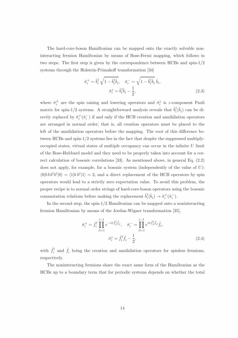
The hard-core-boson Hamiltonian can be mapped onto the exactly solvable non-

interacting fermion Hamiltonian by means of Bose-Fermi mapping, which follows in

two steps. The first step is given by the correspondence between HCBs and spin-1/2

systems through the Holstein-Primakoff transformation [34]

σ+i = b†i

√

1− b†i bi, σ−i =

√

1− b†i bi bi,

σzi = b†i bi −1

2, (2.3)

where σ±i are the spin raising and lowering operators and σzi is z-component Pauli

matrix for spin-1/2 systems. A straightforward analysis reveals that b†i (bi) can be di-

rectly replaced by σ+i (σ−i ) if and only if the HCB creation and annihilation operators

are arranged in normal order; that is, all creation operators must be placed to the

left of the annihilation operators before the mapping. The root of this difference be-

tween HCBs and spin-1/2 systems lies in the fact that despite the suppressed multiply-

occupied states, virtual states of multiple occupancy can occur in the infinite U limit

of the Bose-Hubbard model and they need to be properly taken into account for a cor-

rect calculation of bosonic correlations [33]. As mentioned above, in general Eq. (2.2)

does not apply, for example, for a bosonic system (independently of the value of U):

〈0|b b b†b†|0〉 = 〈1|b b†|1〉 = 2, and a direct replacement of the HCB operators by spin

operators would lead to a strictly zero expectation value. To avoid this problem, the

proper recipe is to normal order strings of hard-core-boson operators using the bosonic

commutation relations before making the replacement b†i (bi) → σ+i (σ−i ).

In the second step, the spin-1/2 Hamiltonian can be mapped onto a noninteracting

fermion Hamiltonian by means of the Jordan-Wigner transformation [35],

σ+i = f †i

i−1∏

β=1

e−iπf†βfβ , σ−i =

i−1∏

β=1

eiπf†βfβ fi,

σzi = f †i fi −1

2, (2.4)

with f †i and fi being the creation and annihilation operators for spinless fermions,

respectively.

The noninteracting fermions share the exact same form of the Hamiltonian as the

HCBs up to a boundary term that for periodic systems depends on whether the total

14

number of bosons N in the system is even or odd 1:

HF = −t∑

i

(

f †i fi+1 +H.c.)

+∑

i

Vi nfi , (2.5)

where nfi = f †i fi is the fermionic occupation operator of site i. This mapping shows

that all thermodynamic properties and real space density-density correlations of hard-

core bosons are identical to those of a system of noninteracting fermions. This is of

course not true for the off-diagonal correlation functions.

2.2 Slater Determinants and Correlation Functions

2.2.1 One-Particle Correlations

In order to compute the one-particle correlations, one can follow the approach described

in Refs. [36, 37]. (Note that in those studies the HCB and spin-1/2 operators were used

indistinctively but consistently with the discussion here.) One can write ρij = b†i bj =

σ+i σ−j and

σ+i σ−j = δij + (−1)δij σ−j σ

+i , (2.6)

so that to compute the one-particle density matrix ρij = 〈ρij〉 one only needs to calcu-

late

Gij = 〈σ−i σ+j 〉 = 〈ΨF |i−1∏

β=1

eiπf†βfβ fif

†j

j−1∏

γ=1

e−iπf†γ fγ |ΨF 〉

= 〈ΨiF |Ψj

F 〉, (2.7)

where

|Ψi(j)F 〉 = f †i(j)

i(j)−1∏

β(γ)=1

e−iπf†

β(γ)fβ(γ) |ΨF 〉, (2.8)

with |ΨF 〉 the many-body ground state of the noninteracting fermionic Hamiltonian

(2.5) we are mapping to. And |ΨF 〉 can be written as Slater determinants in the basis

of Fock states

|ΨF 〉 =N∏

κ=1

L∑

=1

Pκf† |0〉, (2.9)

1For periodic HCB chains, the equivalent noninteracting fermion Hamiltonian satisfies periodic

boundary conditions if the total number of HCBs is odd and antiperiodic boundary conditions if the

total number of HCBs is even [25].

15

with N the number of fermions (bosons in the original Hamiltonian) and L the number

of lattice sites, and Pκ is nothing but the overlap of the site- Fock state and the κth

single-particle eigenstate. Therefore, we are able to consider Pκ as the elements of

a matrix (P)L,N , which is given by the N lowest single-particle eigenfunctions of the

Hamiltonian (2.5)

P =

P11 P12 · · · P1N

P21 P22 · · · P2N...

......

PL1 PL2 · · · PLN

. (2.10)

Notice that in Eq. (2.8), the action of the string of operators on the ground state

just modifies P to create a new Slater-determinant-like matrix Pi(j) in the following

way:∏i−1

β=1 e−iπf†

β fβ = (−1)∑i−1

β=1 f†β fβ generates a sign change on elements Pκ for 6 i,

and the additional f †i creates an extra column to P with the only nonzero element

being Pi,N+1. As such we are able to write Eq. (2.8) in the following form

|ΨαF 〉 =

N∏

κ=1

L∑

=1

Pακf

† |0〉, (2.11)

with α = i, j, and all the elements of the updated matrix (Pα)L,N+1 are given by

Pακ =

−Pκ for < α, κ = 1, . . . , NPκ for ≥ α, κ = 1, . . . , Nδα for κ = N + 1

(2.12)

Now the quantities Gij in Eq. (2.7) can be evaluated by utilizing the matrix repre-

sentation achieved above

Gij = 〈ΨiF |Ψj

F 〉 = det[

(

Pi)†

Pj]

, (2.13)

and further more we obtain the one-particle density matrix 〈ρij〉, from which we also

compute the momentum distribution function by taking the Fourier transformation of

the density matrix, as

nk =1

L

∑

ij

eika(i−j)〈ρij〉, (2.14)

where a is the lattice constant.

16

2.2.2 Noise Correlations

We are also interested in calculating two-particle correlations of HCB systems in quasi-

momentum space [38]. Such quantities, referred to as noise correlations, are defined as

∆kk′ ≡ 〈nknk′〉 − 〈nk〉〈nk′〉 − 〈nk〉(

δk,k′+nK − δkk′)

, (2.15)

where K = 2π/a is the reciprocal lattice vector and n is an integer. The linear term,

proportional to 〈nk〉, has its roots in the commutation relations of bosonic fields and

the requirement of using normal ordered operators if one wants to map time-of-flight

observables to in-situ correlations evaluated before the expansion and restricted to the

lowest band [39]. Here, the last two terms in Eq. (2.15) can be computed using the

approach mentioned in the previous subsection, so we focus on how to compute the

first term

〈nknk′〉 =1

L2

∑

ijlm

eika(i−j)+ik′a(l−m)〈b†i bj b†l bm〉, (2.16)

for which we extend the recipe for calculating the two-point correlations [36, 37] to

obtain four-point correlations and hence the noise correlations.

From the mapping between HCBs and spins one gets the following expression for

the four-point correlation function in terms of spin operators

〈b†i bj b†l bm〉 = δjl〈b†i bm〉+ 〈b†i b

†l bj bm〉

= 2δjl〈σ+i σ−m〉+ (−1)δjl〈σ+i σ−j σ+l σ−m〉, (2.17)

where in the last step we have used Eq. (2.6).

Next we note that last term in Eq. (2.17) can be rewritten as

〈σ+i σ−j σ+l σ−m〉

= δijδlm + (−1)δij δlm〈σ−j σ+i 〉+ (−1)δlmδij〈σ−mσ+l 〉

+ (−1)δij+δlmδim〈σ−j σ+l 〉+ (−1)δij+δlm+δim〈σ−j σ−mσ+i σ+l 〉

= δijδlm + (−1)δij δlmGji + (−1)δlmδijGml

+ (−1)δij+δlmδimGjl + (−1)δij+δlm+δimGjmil, (2.18)

where Gijkl = 〈σ−i σ−j σ+k σ+l 〉. Note that all Gij can be obtained as described in the

previous subsection.

17

Using the Jordan-Wigner transformation in Eq. (2.1), the four-point Green’s func-

tion for the spin-1/2 system can be written as

Gijkl = 〈ΨF |i−1∏

α=1

eiπf†αfα fi

j−1∏

β=1

eiπf†βfβ fj f

†k

k−1∏

γ=1

e−iπf†γ fγ f †l

l−1∏

δ=1

e−iπf†δfδ |ΨF 〉, (2.19)

which using properties of Slater determinants, as described in Refs. [36, 37], can be

computed as

Gijkl = det[

(

Pij)†

Pkl]

, (2.20)

where (Pαβ)L,N+2, with α(β) = i, j, k, l, is given by

Pαβκ =

−P βκ for < α, κ = 1, . . . , N + 1

P βκ for ≥ α, κ = 1, . . . , N + 1δα for κ = N + 2

(2.21)

and (Pβ)L,N+1 is given by Eq. (2.12). This means that to determine each element of

the four-point Green’s function we need to multiply a matrix of dimension (N +2)×L

by a matrix of dimension L × (N + 2) [an operation that scales as (N + 2)2L] and

then compute the determinant of the resulting (N +2)× (N +2) matrix [an operation

that scales as (N + 2)3]. Finally, to compute the full four-point Green’s function, we

need to calculate of the order of L4 nonzero elements; that is, the total computation

time scales as L4[A(N +2)2L+B(N +2)3], with A and B being prefactors for matrix

multiplications and matrix determinants, respectively.

18

3

Noise Correlations of Hard-core

Bosons in 1D Lattices

In this chapter, noise correlations are studied for systems of hard-core bosons (HCBs)

in one-dimensional (1D) lattices. The exact numerical approach introduced in Chap.

2 allows us to study very large lattice sizes and, hence, to performs a systematic finite-

size scaling analysis of observables of interest. We focus on the scaling of the noise

correlations with system size in superfluid and insulating phases, which are generated in

the homogeneous lattice, with period-two superlattices, and with uniformly distributed

random diagonal disorder. For the superfluid phases, the leading contribution is shown

to exhibit a filling-independent scaling proportional to the system size, while the first

subleading term exhibits a filling-dependent power-law exponent.

3.1 Time-of-flight Measurements and Noise Correlations

One of the essential tools to study strongly interacting many-body systems is the detec-

tion of one-particle correlations, e.g. the momentum distribution functions 〈nk〉, whichare the diagonal parts of the Fourier transform of the one-particle density matrix,

〈nk〉 =1

L

∑

ij

eik(Ri−Rj)〈b†i bj〉. (3.1)

They can be experimentally probed by means of time-of-flight measurements, in which

the optical lattice potential is suddenly turned off at τ = 0 and the cloud of atoms

expands for a time of flight before an absorption image is taken to record the observed

19

Figure 3.1: Absorption imaging of an expanding cloud of atoms released from the optical

lattice in time-of-flight measurements. From Ref. [40].

density distribution, as shown in Fig. 3.1. Assuming the interaction is negligible during

the expansion and the time of flight τ is sufficiently long, the average density distri-

bution of the expanding cloud is proportional to the momentum distribution of the

in-trap atoms,

〈n(x; τ)〉 =(m

~τ

)3〈nk〉, (3.2)

where the momentum k is related to the density observation position x by the ballistic

condition k = mx/~τ with m the atomic mass. As we know, long-range order is

associated with peaked momentum distribution. If an optical lattice is present before

the expansion, the resulting density distribution mimics a diffraction grating due to

the properties of the bloch states, leading to interference patterns on the absorption

images with a spatial separation corresponding to the reciprocal lattice vector K of the

underlying lattice. Whereas in the absence of coherence the momentum distribution is

smooth and featureless, as seen in the Mott insulating phase [Figs . 3.2(a) and 3.2(b)].

Studies of the momentum distribution of harmonically trapped HCBs has been

performed in several recent works [36, 37, 41–43]. The zero-momentum peak of the

momentum distribution in a superfluid was found to scale with the square root of the

system size [26] while it saturates in the Mott insulating [44, 45] and disordered [46]

phases. The latter behavior is a result of the short-range correlations present in the

insulating phases.

Remarkably, it was also recently proposed that second-order correlations can be ex-

tracted by analyzing the atomic shot noise in the time-of-flight images of an expanding

20

Figure 3.2: (a) Single shot absorption image of a Mott insulator and (b) a section through

the center of the image. (c) Atomic shot noise obtained by processing many independent

images, and (d) a section showing the correlation peaks. From Ref. [40].

cloud [38]. It is nothing but the density covariance

∆(x,x′) = 〈n(x)n(x′)〉 − 〈n(x)〉〈n(x′)〉, (3.3)

where the first term, referred to as the density-density correlation, can be written in

terms of normally ordered field operators as

〈n(x)n(x′)〉 = 〈Ψ†(x)Ψ†(x′)Ψ(x)Ψ(x′)〉+ δ(x− x′)〈n(x)〉. (3.4)

Similarly, following the ballistic expansion condition and up to a constant factor and a

self-correlation term, the density covariance (3.3) can be mapped to the noise correlation

∆kk′ in the momentum space,

∆kk′ ≡ 〈nknk′〉 − 〈nk〉〈nk′〉 − 〈nk〉

(

δk,k′+nK − δkk′

)

, (3.5)

with n an integer. The large fluctuations contained in the absorption image are re-

lated to the intrinsic quantum noise by means of Hanbury-Brown-Twiss effect and they

reflect the underlying spatial order of the system that is not revealed in the average

density distribution [40]. Therefore, these second-order correlations offer information

not only in complement to the momentum distribution but beyond them, including the

fundamental statistics of the atomic particles, i.e., the bunching (antibunching) effect of

bosons (fermions). Shortly after the theoretical proposal [38], noise correlations were

21

measured in experiments with bosons in 3D optical lattices [40] and with attractive

fermions [47]. In the former experiment, despite of a featureless momentum distribu-

tion, noise correlation peaks of bunching type were observed in an Mott insulator [Figs.

3.1(c) and 3.1(d)].

Our goal in this work is to explore the scaling of the noise correlations in various

ground-state phases of 1D hard-core-boson-lattice systems. We consider the homoge-

neous case, systems with an additional period-two superlattice potential, and disordered

systems with a uniform random distribution of local potentials. There are three ground-

state phases on which we will focus our present study, which are the superfluid phase,

the Mott-insulating or charge-density-wave phase, and the Bose-glass phase associated

with disorder-induced localization. Those phases can be obtained in the various afore-

mentioned background potentials. In the superfluid phase, we show that the leading

contribution to the noise correlation peaks scales linearly with the size of the system,

independently of the density and of the absence or presence of a superlattice poten-

tial, while the first subleading term does depend on both. As expected, for the Mott

and the Bose-glass phases, which are both insulating, the scaling of the peaks shows an

asymptotic value that depends on the density and strength of the background potential

but that is independent of the system size.

3.2 Homogeneous System

The Hamiltonian to describe HCBs loaded in 1D periodic lattice with homogeneous

(zero) external potential is simply

HHCB = −t∑

i

(

b†i bi+1 +H.c.)

. (3.6)

We should stress that, for all HCB systems considered in the rest of the chapter, peri-

odic boundary conditions are always implemented; that is, for the equivalent fermionic

Hamiltonians, periodic or antiperiodic conditions are selected depending on the number

of particles in the lattice.

In Fig. 3.3, we show a typical noise correlation pattern for a strongly interacting

superfluid system. It was calculated in a periodic lattice with 200 sites at half-filling.

There are three features in that pattern that are apparent. First, a very large peak

appears at k = k′ = 0, reflecting the presence of quasicondensation in the system.

22

Figure 3.3: Noise correlations as a function of k and k′ for a homogeneous system with

100 HCBs in 200 lattice sites.

Replicas of this peak also appear at integer multiples of the reciprocal lattice vector

K. Second, a line of maxima can be found for k = k′ due to the usual bunching in

bosonic systems. Finally, dips are seen along the lines k, 0 and 0, k′, which are related

to the quantum depletion in the system. These features have been discussed in detail in

Ref. [48] in the more general context of Luttinger liquids, for which HCBs correspond

to a limiting case.

As a function of the filling factor ρ = N/L, the evolution of the noise correlations

along the line k, 0 is depicted in Fig. 3.4. The dips around the k = 0,±K peaks are

more clearly seen in that figure. As noted in Ref. [33], we find that the maximum value

of ∆00 occurs for ρ > 0.5, making evident the breakdown of the particle-hole symmetry

for this observable.

In what follows, we will focus on the scaling of the ∆00 for different densities. For

the k = 0 peak of the momentum distribution function, it is well known that the

power-law decay of the one-particle correlations results in a nk=0 ∼√L scaling [26]. In

Fig. 3.5, we show the scaling of ∆00 for three different densities in our periodic systems.

To numerically find the scaling with system size, we assume that

∆00 = aLx + bLy, (3.7)

23

Figure 3.4: Noise correlations for k′ = 0 as k and ρ are changed for a system with

L = 200.

where x and y (y < x) describe the leading and subleading terms, respectively, and

a and b are coefficients that, together with x and y, are determined by means of

a numerical fit. The results obtained for those four fitting parameters are given in

Table 3.1.

ρ = 0.25 ρ = 0.5 ρ = 0.75

a 0.17779(2) 0.21(9) 0.16(1)

x 1.00041(2) 1.01(3) 1.010(8)

b −1.049(4) 0.15(7) 0.534(6)

y −0.099(1) 0.8(1) 0.59(2)

Table 3.1: Fitting parameters for the homogeneous case.

Table 3.1 shows that the leading term is essentially linear in all cases, while the

exponent of the power law of the subleading term does depend on the filling factor and

was found to be quite close to one around half-filling. This means that in ultra-cold gas

experiments one would need to reach large systems sizes to be able to clearly observe

the linear scaling of the noise correlation peaks around half-filling, while this scaling

would be more easily observed far away from half-filling.

24

100 150 200 250 300 35010

20

30

40

50

60

70

80

90

100 =0.25 =0.5 =0.75

00

L

Figure 3.5: Scaling of the noise correlations ∆00 for three different densities, ρ =0.25,

0.5 and 0.75. The solid lines are numerical fits in the form of Eq. (3.7) and the results (see

text) show a leading-order linear behavior.

3.3 Period-two Superlattice

We now consider the case in which an additional lattice, with twice the periodicity of

the original lattice, is superimposed to the system (a superlattice). In this case, the

on-site potential in Hamiltonian (2.1) has the form

Vi = V (−1)i, (3.8)

with V representing its strength. As discussed in Ref. [44, 45], the effect of a period-

two superlattice is to open a gap of magnitude 2V in the energy spectrum, splitting

the original band into two bands. As a result, besides the usual insulating phases at

ρ = 0, 1, the half-filled system in the ground state also exhibits insulating behavior. As

opposed to the ρ = 0, 1 insulators, the ρ = 0.5 (Mott) insulator does exhibit nonzero

density fluctuations and a finite correlation length.

Figure 3.6 shows the noise correlation pattern for the ρ = 0.5 insulator with V = 1t.

Broad peaks can be clearly seen along the line k = k′, and those are characteristic of the

noise correlations in the fractional Mott phase. They contrast with the sharp peaks seen

in the noise correlations of the superfluid regime studied in the previous section. The

suppressed height of the peaks in Fig. 3.6 is a signature of the destruction of the quasi-

long-range coherence in the half-filled Mott system. At this critical filling, the power-

25

Figure 3.6: Noise correlations for the fractional Mott phase in the half-filled system in

the presence of period-two superlattice for L = 200.

law decay of the one-particle correlations present in the absence of the superlattice is

substituted by an exponential decay ρij ∼ exp(−|i − j|/ξ), for which the correlation

length ξ was found to be ξ ∼ 1/V for small values of V (V < t) and ξ ∼ 1/√V for large

values of V (V > t) [45]. As long as the lattice sizes are sufficiently large (L≫ ξ), the

absence of quasi-long-range coherence should be clearly observed in the scaling of the

noise correlations in those systems.

In the presence of the superlattice potential, additional features emerge in the noise

correlations for k = k′ ± π/a. Those can actually be used to distinguish the fractional

insulator from the integer Mott insulator as both have suppressed ∆00 peaks but only

the former has a structure in the noise correlations for k = k′ ± π/a.

In Fig. 3.7, we present a unified view of the behavior of the noise correlations for

different systems with a superlattice potential. There we plot ∆k0 as a function of ρ

and k for four different values of V . Figure 3.7 shows that as V increases from 1t to 4t,

the intensity of the central peak decreases for all fillings. However, the suppression is

more dramatic around half-filling. The additional unique signature of the presence of

a superlattice potential is the structure that can be found at ka = ±π. It is usually a

positive peak for densities below 0.5 and becomes a dip right after the density increases

beyond the fractional filling insulating phase. This peak-to-dip transition was discussed

in detail in Refs. [49, 50], where in the limit V → ∞ one can show analytically that

26

Figure 3.7: Noise correlations ∆k0 as a function of k and the filling factor for superlattice

systems with (a) V = 1t, (b) V = 2t, (c) V = 3t, and (d) V = 4t. L = 200 in all cases.

∆00 and ∆±πa0 have different signs for N = L/2 + 1.

The behavior of ∆πa0 as a function of the filling factor and for different values of V

can be better seen in Fig. 3.8. Interestingly, we find that, in addition to the peak to

0.0 0.2 0.4 0.6 0.8 1.0-2

-1

0

1

2

3

4

5

0.0 0.5 1.0

-1

0

1

2

/a,0

V=0.5t V=1t V=2t V=4t

/a,0

Figure 3.8: The sublattice peak ∆π

a,0 as a function of ρ for four different values of V in

systems with 200 sites. The inset shows the same quantity for systems with 100 sites.

27

100 150 200 250 300 350

0

20

40

60

80

100

100 200 3003.35

3.40

3.45

3.50

100 200 3000

1

2

=0.25 =0.75

00

L

=0.5

00

L

/a,0

L

=0.25

Figure 3.9: Scaling of ∆00 for ρ = 0.25 and ρ = 0.75 in systems with V = 1t and lattices

with 200 sites. The top inset shows results for the same systems in the fractional (ρ = 0.5)

Mott-insulating phase. The bottom inset shows scaling of the sublattice peak ∆π

a0 for

ρ = 0.25 in the same systems. Solid lines are numerical fits to the results, exhibiting a

leading linear scaling with L in all superfluid cases.

dip transition around ρ = 0.5, there are other dip to peak and peak to dip transitions

for higher densities. Those are only apparent for sufficiently large system sizes (beyond

the ones studied in Refs. [49, 50]). The inset in Fig. 3.8 shows that for a smaller system

size with only 100 sites ∆πa0 is always negative for ρ > 0.5.

Now that the generic features of the noise correlations in a superlattice potential

have been reviewed, we focus on the scaling of the peaks with system size. In the

fractional insulating regime, one expects that the exponential decay of correlations

should lead to a saturation of the noise correlation peaks. This is, indeed, what we

find, and an example is depicted in the top inset in Fig. 3.9 for half-filled systems with

V = t.

In the superfluid phases, on the other hand, it has been shown that one-particle

correlations decay with exactly the same power law as the homogeneous system [45].

Hence, we expect to find the same leading order scaling of ∆00 that was discussed for

homogeneous systems in the previous section. This result can be seen in the main panel

of Fig. 3.9, and it can also be seen for the ∆πa0 peak, for ρ = 0.25, in the bottom inset.

Assuming the same scaling ansatz in Eq. (3.7), but in the presence of the superlattice

only used for the superfluid phases, we obtain the values depicted in Table 3.2 for the

28

fitting parameters.

k = 0 k = π/a

ρ = 0.25 ρ = 0.75 ρ = 0.25

a 0.15928(6) 0.090(1) 0.00716(2)

x 0.99023(6) 1.045(1) 1.0133(3)

b −5.2(3) 0.5793(5) −0.03891(9)

y −0.71(1) 0.636(2) 0.417(1)

Table 3.2: Fitting parameters for the superlattice case.

As expected, we find that the leading terms of the noise correlation peaks are also

of order L for both ∆00 and ∆πa0. Similar to the homogeneous case, the leading linear

scaling of those peaks is better seen at low densities where finite-size effects have been

found to be smaller because the subleading term vanishes with increasing system size.

3.4 Disordered Lattice

The disordered case is simulated by a random on-site potential of the form

Vi = δǫi, (3.9)

where δ represents the strength of disorder and {ǫi} are a set of random numbers

between -1 and 1 selected with a uniform probability distribution. For our disorder

calculations we usually average over between 128 and 256 disorder realizations.

For 1D noninteracting fermionic systems, the presence of disorder is known to lead

to Anderson localization. This is an insulating phase in which correlations decay expo-

nentially while the system remains compressible; that is, no gap is present in the energy

spectrum. Since hard-core bosons can be mapped to noninteracting fermions, the same

is known to be true for the former, and such a phase presented in the Bose systems is

known as Bose-glass phase. We should note that despite the fact that the one-particle

correlations of hard-core bosons are in general different from those of noninteracting

fermions, they also decay exponentially. This is shown in Fig. 3.10, where we present

one-particle correlations ρx (averages of ρij = 〈b†i bj〉 over i, j for fixed x = |j − i|) as

a function of x for systems with different disorder strengths. One should note that

the exponential decay always sets in beyond a certain distance, which decreases as the

29

0 50 100 150 20010-8

10-6

10-4

10-2

100

=0 =1t =2t =3t =4t

x

x/a

Figure 3.10: The decay of off-diagonal one-particle correlations in half-filled systems with

L = 500, characterized by different disorder strength. The disorder averaging is performed

over 128 realizations for all δ 6= 0 cases. Solid lines depict exponential decay, except for

the homogeneous (δ = 0) system, where the line depicts the known power law√x. Note

the log-linear scale.

strength of the disorder increases; that is, small systems with weak disorder may behave

as superfluids.

From the previous discussion and the results in Fig. 3.10 one expects that, for

any given system size, the height of the noise correlation peaks should decrease with

increasing disorder strength and the peaks should become broader. This can be seen

in Fig. 3.11, where we show the noise correlations ∆kk′ for four different disordered

strengths in systems with 100 sites. The pattern for the δ = 1 case resembles that of

a homogeneous superfluid system (Fig. 3.3), while for larger values of δ they display

more similarities with the fractional Mott-insulating phase in the half-filled superlattice

systems, with a clear broadening of the peaks at k = k′. (Of course, no additional

feature appear for k = k′ ± π/a in the disordered case.)

A comparison between the cross-sectional view (for k′ = 0) of the noise correlations

in all three phases discussed previously, namely, the superfluid, fractional Mott, and

glassy phases, is shown in Fig. 3.12. This comparison makes evident (i) the suppression

of the ∆00 peak in the fractional Mott and glassy phases, (ii) the fact that the two

insulating phases can be distinguished by the superlattice-induced features at k = k′±π,and (iii) that the disordered Bose-glass and the superfluid phase exhibit the same

30

Figure 3.11: Disorder-averaged noise correlations as a function of k and k′ for systems

with different disorder strength δ =(a) 1t, (b) 2t, (c) 3t, and (d) 4t. N = 50 and L = 100

for all cases and the average was performed over 128 disorder realizations.

-2 -1 0 1 2

0

5

10 disordered

k0

ka/

0

1

2

3

superlattice

0204060

homogeneous

Figure 3.12: Noise correlations with fixed k′ = 0 for three half-filled systems with

L = 200. The superfluid phase, the fractional Mott phase, and the Bose-glass phase

are associated with the homogeneous, period-two superlattice (V = 2t), and disordered

(δ = 2t) cases, respectively. The average is performed over 256 disorder realizations.

31

50 100 150 2000

10

20

30

40

50

00

L

=0.5t =1t =2t

Figure 3.13: Scaling of the noise correlations ∆00 for three different values of δ in half-

filled systems.

satellite dips accompanying the ∆00 peaks, while the dips vanish rather quickly in the

fractional Mott phase.

Similar to the behavior of the fractional Mott phase, one also expects that as the

system size increases for any nonzero value of the disorder strength, the ∆00 will sat-

urate to a size-independent value that will only be a function of the filling factor and

the disorder strength. This behavior is shown in Fig. 3.13 for three different values of

the disorder strength and for systems with up to 200 sites.

Finally, we study how the ∆00 peak in the noise correlations behaves as a function

of the disorder strength for a fixed size of the lattice. Since for δ = 0 we have already

shown that such a peak diverges with system size, in the following we analyze how ∆00

decreases as the disorder strength increases.

In Fig. 3.14, we show ∆00 as a function of δ for two different system sizes. Three

different regimes can be clearly identified. (i) For small values of δ, ∆00 approximately

stays constant with the increase of δ, which can be understood to be a consequence

of a correlation length that exceeds the system size. As seen in Fig.3.14, that region

decreases as the system size increases. (ii) As δ increases even further, a power-law

decay develops in ∆00, and the region over which such a power law can be seen increases

with system size as regime (i) is suppressed. In our fits, we find the power law ∆00 ∼ δ−γ

to have an exponent γ ∼ 1.78(2), but it is still influenced by some finite-size effects. In

32

0.1t 1t 10t1

10

100

10t

1

10

0.1t 1t 10t1

10

L=100 L=200

L=100 L=200 L=300

v

Figure 3.14: Noise correlation peaks ∆00 as a function of disorder strength in two half-

filled disordered systems with L =100 and 200, respectively. The solid line shows a power-

law fit ∆00 ∼ δ−γ , with γ = 1.78(2) in the range from δ = t to 3t for L = 200. The

top inset shows ∆00 as a function of V in three half-filled period-two superlattices. The

solid line depicts a power law with an exponent γ = 0.874(5). The bottom inset shows the

asymptotic behavior for large values of δ; the dotted line marks the analytical result in the

limit of infinite disorder.

order to gain further understanding of the power-law decay of the height of this noise

peak in insulating phases, we have studied the behavior of ∆00 vs V in the fractional

Mott phase in a superlattice, for which we can study larger systems sizes. We find

that ∆00 ∼ V −γ with an exponent of 0.874(5), which is different from the one for the

disordered system. These results clearly show that the power-law decay of ∆00 as one

enters an insulating phase depends on the perturbation creating the insulator, i.e., it is

not universal. (iii) Finally, for very strong disorder, ∆00 saturates to a nonzero value.

This asymptotic behavior is found to agree with the analytical value in the δ → ∞limit, computed using

∆00 = ρ(ρ+ 1), (3.10)

which was derived in Ref. [49]. Equation (3.10) shows that ∆00 only depends on the

filling factor and also makes explicit the absence of particle-hole symmetry for this

observable in HCB systems. This third regime is robust against the disorder variance,

something that follows from the fact that the correlation length is of the order of or

smaller than the lattice spacing a.

33

4

Quantum Phase Transition in

Incommensurate Lattices

In this chapter, we study the problem of one-dimensional (1D) hard-core bosons (HCBs)

with pseudorandom disorder generated by imposing two-color lattices with periods that

are mutually incommensurate1. Even in the absence of interactions, 1D quasiperiodic

systems exhibit a localization-delocalization transition. Finite-size scalings of the mo-

mentum distribution and noise correlations are performed to study Mott insulator, Bose

glass, and superfluid quantum phases in such systems. The exponents of the correlation

functions at the superfluid to Bose glass (SF-BG) transition are found to be approxi-

mately one half of the ones that characterizes the superfluid phase. The derivatives of

the peak intensities of the correlation functions with respect to quasiperiodic disorder

are shown to diverge at the SF-BG critical point. This behavior does not occur in

the corresponding free fermion system, which also exhibits an Anderson-like transition

at the same critical point, and thus provides a unique experimental tool to locate the

phase transition in interacting bosonic systems. We also report on the absence of pri-

mary sublattice peaks in the momentum distribution of the superfluid phase for special

fillings.

1This work was done during the author’s year-long internship at NIST in Gaithersburg, MD. It was

in collaboration with Dr. Charles W. Clark (NIST/JQI), who hosted my stay in NIST, Dr. Indubala

I. Satijia (George Mason University), and Dr. Ana Maria Rey (JILA).

34

4.1 Quasiperiodic Systems and Disorder-induced Phase

Transition

Since the celebrated work of Anderson [51] and others about half a century ago, the

subject of disorder and quantum phase transitions induced by disorder continues to

attract interest [52]. In spite of being intensively studied, the interplay between inter-

actions and disorder remains an open frontier. In recent years, a new impetus toward

the understanding of disorder systems has emerged in the context of ultracold atomic

systems because of their extraordinary degree of tunability. In those systems, it is now

possible to control the degree of disorder either by imprinting speckle patterns [53, 54]

or by superimposing a secondary lattice on the main lattice to generate a quasiperi-

odic potential [55–58]. Using those techniques, Anderson localization has already been

observed in 1D [53, 55, 58]. At the same time, the possibility of exploring strongly

interacting regimes with ultra-cold atoms has been demonstrated by observation of the

superfluid to Mott insulator transition [13, 15–17], and the realization of the Tonks-

Girardeau gas, i.e., a gas of impenetrable (hard-core) bosons (HCBs), in 1D [19, 22, 59].

The combined investigation of the effect of disorder and correlations in low-dimensional

systems is therefore a window that is now open for experimental exploration [18] and

has driven many recent investigations [33, 60–62].

In this chapter we revisit the problem of 1D HCBs with pseudorandom disorder gen-

erated by imposing two-color lattices with periods that are mutually incommensurate.

Even in the absence of interactions, one-dimensional quasiperiodic systems exhibit a

localization-delocalization transition. In contrast to truly random 1D systems where

states are localized irrespective of the strength of disorder, quasiperiodic systems ex-

hibit a quantum phase transition from extended to localized at a finite strength of

the quasiperiodic disorder. In the interacting soft-core regime, several studies have

addressed the phases that result from the interplay between pseudorandom disorder

and strong correlations. Those studies have utilized different computational techniques

such as exact diagonalization [63, 64], quantum Monte Carlo simulations [65], and the

density-matrix renormalization group method [66, 67]. A recent comprehensive discus-

sion of these, and other, results can be found in Ref. [18]. In this chapter, we perform

an exact numerical study of ultracold bosons in the hard-core regime, as well as spinless

fermions, and investigate the effects of the interplay between disorder and interactions

35

in the momentum distribution and noise correlations of those systems. These two ob-

servables can be experimentally probed through time-of-flight measurements [38, 40].

4.1.1 Incommensurate Lattice

One-dimensional HCBs in incommensurate superlattices, within the one-band approx-

imation, are described by the following Hamiltonian:

HHCB = −t∑

j

(b†j bj+1 +H.c.) +∑

j

Vj nj, (4.1)

where

Vj = 2λ cos(2πσj + δ),

in which the parameter λ is proportional to the intensity of the lasers used to create the

secondary lattice, σ is the ratio between the wave vectors of the two lattices, and δ is a

generic phase factor. Here, we choose δ to be zero without lost of generality. Finally, we

note that the hopping parameter is set to one (t = 1) and periodic boundary conditions

are considered throughout this chapter.

Quasiperiodic lattices are characterized by an irrational σ, which results from the

incommensurate periodicity of the two superimposed lattices. In our studies, we choose

σ to be the reverse golden ratio, σ = (√5 − 1)/2

.= 0.61803.... This choice is moti-

vated by the fact that the golden mean is considered to be the most irrational number

[61, 68] and has simple number theoretical properties. In our numerical calculations, σ

is approximated by the ratio of two consecutive Fibonacci numbers FM−1/FM , where

the Fibonacci numbers are defined by the recursion relation Fi+1 = Fi + Fi−1, with

F1 = F0 = 1. Within the approximation followed in this manuscript, model (4.1) on a

quasiperiodic superlattice reduces to a model on a periodic superlattice whose proper-

ties are well known (σ is rational). The latter nevertheless captures the localization-

delocalization transition exhibited by the quasiperiodic system [44, 69].

4.1.2 Localization-delocalization Transition

As mentioned before, two-color superlattices characterized by an irrational σ are in-

termediate between periodic and fully random lattices, and exhibit a metal-insulator

transition in one dimension. The critical point λc = t describes the onset of local-

ization. Below criticality (λ < λc), single-particle states are extended, namely, they

36

are Bloch-like states. Above the critical point, single-particle states are exponentially

localized with localization length ξ = ln(λ)−1 [70].

In the extended phase, the energy spectrum consists of a set of bands (it becomes a

Cantor set at the localization threshold). The gaps are located at k = ±nσ(mod 1)π/a

in the first Brillouin zone, indexed by an integer n. Note that as n increases the width

of the gaps narrows. As a consequence of our selection of σ = FM−1/FM , the single-

particle spectrum consists of FM bands and FM − 1 gaps. The filling factor ρ = N/L

in a many-body system, where N is the number of particles and L the number of sites,

is then a control parameter that tunes transitions between different phases. For fillings

ρ = nσ(mod 1) and ρ = 1 − nσ(mod 1), the ground state of HCBs in the extended

regime is a Mott insulator. This insulating state is incompressible and it is also referred

to as an incommensurate insulator [33, 61, 65]. The fact that the system is insulating

at those fillings can be understood in a way that the conduction bands in the fermionic

system, to which the HCBs can be mapped, are filled [33, 61]. For all other fillings,

the ground state is a superfluid. To be able to observe the fractional Mott insulating

phases, the lattice size must be identical to (or multiple integers of) the period of

the incommensurate potential, which means that we choose L = FM while having

σ = FM−1/FM . In our study, we consider lattices with L =34, 55, 89, 144, and 233.

For λ > λc, i.e., in the localized regime, the ground state remains an incompressible

insulator for fillings ρ = nσ(mod 1) and ρ = 1 − nσ(mod 1). For all other fillings, on

the other hand, the ground state is a Bose glass. The Bose-glass phase is a compressible

insulating state where the absence of transport is the result of localization [18].

4.2 Quantum Correlations: Scaling Analysis

In this section, we perform a finite-size scaling study of the momentum distribution as

well as the noise correlations in different regimes. Typical momentum profiles and noise

correlation patterns are shown in Fig. 4.1. They were calculated on a system with 200

sites at half filling and for three different values of λ representing the superfluid phase,

the critical point, and the localized phase.

The momentum distribution reflects the quantum coherence of the system. It ex-

hibits a sharp diffraction pattern in the extended regime (superfluid phase) and a flat

profile in the Bose-glass and Mott insulating phases [see Fig. 4.1(a)]. The interference

37

0.2 0.4 0.6 0.8-0.2

-0.1

0.0

0.1

0.2 0.4 0.6 0.80.00

0.25

0.50

0.75

0 /4 /2 3 /4

-2.5

0.0

2.5

5.0

7.5

10.0

12.5

=0.5 =1 =1.5

n(k)

ka

(a)0 /4 /2 3 /4

-20

-10

0

10

20

30

40

50

(b) =0.5 =1 =1.5

k0

ka

Figure 4.1: (a) Momentum distribution n(k) and (b) noise correlations ∆k0, of HCBs,

as a function of k for three different values of λ. In all cases L = 233, N = 166, and

σ = 144/233. The insets in (a) and (b) show the set of sublattice peaks in the momentum

distribution and noise correlations, respectively.

pattern is characterized by a peak at k = 0 and additional sublattice peaks at the cor-

responding reciprocal lattice vectors. In the quasiperiodic lattice under consideration,

they are found at ka = ±nσ(mod 1)2π and ka = ±(1 − nσ)(mod 1)2π. In general,

only peaks associated with the main reciprocal lattice vectors, n = 1, are distinguish-

able. The k = 0 peak is the sharpest peak and signals the superfluid character of the

extended phase.

The noise correlation pattern contains information of the momentum-momentum

correlations and is also known as Hanbury Brown–Twiss interferometry. It exhibits

interference peaks in all phases, even in the insulating ones. In contrast to the momen-

tum distribution, the noise correlation fringes have their root in the quantum statistics

of the particles. For bosonic systems, the peaks are positive and are a manifestation of

bunching. For fermionic systems, they are negative and signal antibunching [38, 40].

The height of the noise correlation peaks and their underlying background signif-

icantly vary in the various quantum phases studied here. For example, a negative

background is found in the superfluid regime. Also, the sublattice peaks disappear in

the Mott insulting phase which occur at unit filling. The insets in Figs. 4.1(a) and

4.1(b) show the most noticeable sublattice peaks in our systems.

In Fig. 4.2 we plot the central peak of the momentum distribution function nk=0

(a) and the noise correlation peak ∆00 (b) as a function of the system size L for various

values of λ. Note that the filling factor is fixed at ρ = 0.5 so that a superfluid state is

associated with the λ < 1 cases. The distinction in the scaling behavior in the extended

38

20 100 600

1

10

20 100 1000

2

34567

30 100 200 300

5

10

15

=0.5=0.6=0.8=0.9

=1

=1.1=1.2=1.5=2

n k=0

L

(a)

=1/3 =1/2

L

20 100 6001

10

100=0.5=0.6=0.8=0.9

=1

=1.1=1.2=1.5=2

00

L

(b)

=1/3 =1/2

L

Figure 4.2: Scaling of (a) nk=0 and (b) the central peak ∆00 in half-filled systems for

various values of λ. The inset in (a) depicts the scaling of nk=0 for λ = λc and up to

larger system sizes. The black dotted lines are power-law fits to the data, from which the

exponents (see text) indicate the distinction between the extended regime, the transition

point, and the localized regime.

regime, at the transition point, and in the localized regime is apparent. One can see

that both nk=0 and ∆00 exhibit power-law scaling in the superfluid phase as well as

at criticality, while in the Bose-glass phase they remain essentially unchanged with

changing L.

In Fig. 4.2(a), the four sets of values of nk=0 vs L for λ =0.5,0.6,0.8, and 0.9 exhibit

exponents 0.503±0.001, 0.496±0.002, 0.462±0.007, and 0.42±0.01, respectively, which

are compatible with the well-known nk=0 ∼√L scaling for HCBs in the superfluid

regime, where the quasi-long-range order is present in the one-particle correlations. In

Fig. 4.2(b), the exponents for ∆00 in the extended regime are 0.903±0.003, 0.878±0.004,

0.799 ± 0.007, and 0.72 ± 0.01, also for λ =0.5, 0.6, 0.8, and 0.9, respectively. These

results are compatible with the linear behavior ∆00 ∼ L reported in Ref. [71], where

the superfluid phase of the homogeneous system and the period-2 lattice was studied.

Overall, the results in the extended regime are consistent with the fact that for λ < 1

the system is a Luttinger liquid with the Luttinger parameter K = 1 [18]. On the other

hand, for λ > 1, Fig. 4.2 shows that both nk=0 and ∆00 do not scale with system size,

which is a demonstration of the presence of exponentially decaying correlations in the

Bose-glass phase, and hence the lack of Luttinger liquid behavior.

The behavior at the critical point is the most interesting one, as the system is not

expected to be described by the Luttinger liquid theory. Still, we find a power-law

39

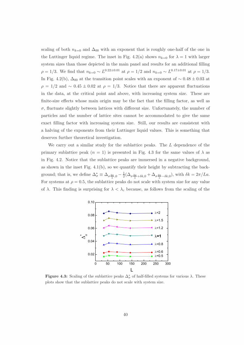
scaling of both nk=0 and ∆00 with an exponent that is roughly one-half of the one in

the Luttinger liquid regime. The inset in Fig. 4.2(a) shows nk=0 for λ = 1 with larger

system sizes than those depicted in the main panel and results for an additional filling

ρ = 1/3. We find that nk=0 ∼ L0.22±0.01 at ρ = 1/2 and nk=0 ∼ L0.17±0.01 at ρ = 1/3.

In Fig. 4.2(b), ∆00 at the transition point scales with an exponent of ∼ 0.48 ± 0.03 at

ρ = 1/2 and ∼ 0.45 ± 0.02 at ρ = 1/3. Notice that there are apparent fluctuations

in the data, at the critical point and above, with increasing system size. These are

finite-size effects whose main origin may be the fact that the filling factor, as well as

σ, fluctuate slightly between lattices with different size. Unfortunately, the number of

particles and the number of lattice sites cannot be accommodated to give the same

exact filling factor with increasing system size. Still, our results are consistent with

a halving of the exponents from their Luttinger liquid values. This is something that

deserves further theoretical investigation.

We carry out a similar study for the sublattice peaks. The L dependence of the

primary sublattice peak (n = 1) is presented in Fig. 4.3 for the same values of λ as

in Fig. 4.2. Notice that the sublattice peaks are immersed in a negative background,

as shown in the inset Fig. 4.1(b), so we quantify their height by subtracting the back-

ground; that is, we define ∆∗σ ≡ ∆σ 2π

a,0 − 1

2(∆σ 2πa+δk,0 +∆σ 2π

a−δk,0), with δk = 2π/La.

For systems at ρ = 0.5, the sublattice peaks do not scale with system size for any value

of λ. This finding is surprising for λ < λc because, as follows from the scaling of the

0 50 100 150 200 250 300

0.02

0.04

0.06

0.08

0.10

=2

=1.5

=1.2

=1

=0.8

=0.6=0.5

LFigure 4.3: Scaling of the sublattice peaks ∆∗

σ of half-filled systems for various λ. These

plots show that the sublattice peaks do not scale with system size.

40

0 50 100 150 200 250

1

2

3

4

5

6

7

8

L

=0.5 =1 =2 =4

(a)

0 50 100 150 200 250

0.00

0.02

0.04

0.06

0.08

0.10

(b) =0.5 =1 =2 =4

LFigure 4.4: (a) Central noise correlation peak ∆00 and (b) the sublattice peak ∆∗

σ as a

function of L in systems at incommensurate filling ρ = σ.

∆00 peak, quasi-long-range order is present in the system in that regime. On the other

hand, the absence of those peaks is expected in the glassy phase where correlations

decay exponentially. Further analysis reveals that, within a range of filling factors from

ρ = 1 − σ to ρ = σ, ∆∗σ does not scale with system size in the superfluid phase. This

will be discussed in detail in Sec. 4.4.

At the incommensurate fillings ρ = nσ(mod 1) and ρ = 1 − nσ(mod 1), a Mott

insulating phase rather than a superfluid one is present for all λ 6= 0. We then study

the noise correlation peaks in systems with incommensurate filling ρ = σ. In Fig. 4.4,

both ∆00 and ∆∗σ are plotted as a function of L for various values of λ. The absence of

scaling is apparent in both noise correlation peaks for all regimes. For those fillings, nk

and the noise correlations do not distinguish the localization delocalization transition

that occurs at λc.

4.3 Quantum Phase Transition

In order to gain a better understanding of the disorder-induced phase transition and

its signatures in our strongly interacting system, we study the behavior of the noise

correlations in the vicinity of the critical point. Our study involves monitoring the peak

intensities and their derivatives as the strength of the quasiperiodic order is tuned.

Figures 4.5(a) and 4.5(b) depict the results for the central peak and the primary

sublattice peak, respectively, as a function of λ in a half-filled system. With the increase

of disorder, the height of the central peak (∆00) decreases and attains an asymptotic

value ∆00 = ρ(ρ+1) as λ→ ∞ [33, 71], while the height of the sublattice peak increases

41

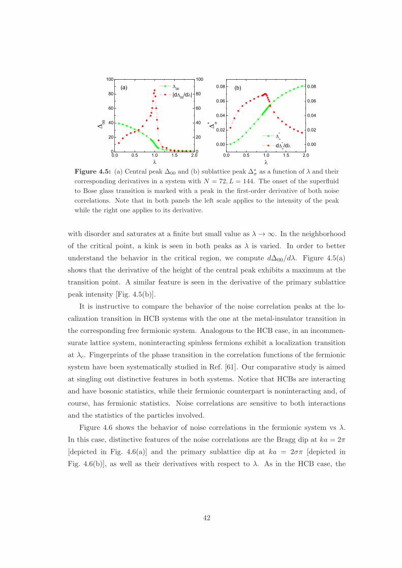
0.0 0.5 1.0 1.5 2.00

20

40

60

80

100

0

20

40

60

80

100

00

|d 00/d |(a)

0.0 0.5 1.0 1.5 2.0

0.00

0.02

0.04

0.06

0.08

0.00

0.02

0.04

0.06

0.08

*

d */d

(b)

Figure 4.5: (a) Central peak ∆00 and (b) sublattice peak ∆∗

σ as a function of λ and their

corresponding derivatives in a system with N = 72, L = 144. The onset of the superfluid

to Bose glass transition is marked with a peak in the first-order derivative of both noise

correlations. Note that in both panels the left scale applies to the intensity of the peak

while the right one applies to its derivative.

with disorder and saturates at a finite but small value as λ→ ∞. In the neighborhood

of the critical point, a kink is seen in both peaks as λ is varied. In order to better

understand the behavior in the critical region, we compute d∆00/dλ. Figure 4.5(a)

shows that the derivative of the height of the central peak exhibits a maximum at the

transition point. A similar feature is seen in the derivative of the primary sublattice

peak intensity [Fig. 4.5(b)].

It is instructive to compare the behavior of the noise correlation peaks at the lo-

calization transition in HCB systems with the one at the metal-insulator transition in

the corresponding free fermionic system. Analogous to the HCB case, in an incommen-

surate lattice system, noninteracting spinless fermions exhibit a localization transition

at λc. Fingerprints of the phase transition in the correlation functions of the fermionic

system have been systematically studied in Ref. [61]. Our comparative study is aimed

at singling out distinctive features in both systems. Notice that HCBs are interacting

and have bosonic statistics, while their fermionic counterpart is noninteracting and, of

course, has fermionic statistics. Noise correlations are sensitive to both interactions

and the statistics of the particles involved.

Figure 4.6 shows the behavior of noise correlations in the fermionic system vs λ.

In this case, distinctive features of the noise correlations are the Bragg dip at ka = 2π

[depicted in Fig. 4.6(a)] and the primary sublattice dip at ka = 2σπ [depicted in

Fig. 4.6(b)], as well as their derivatives with respect to λ. As in the HCB case, the

42

0.1

0.2

0.3

0.4

0.5

0.6

0.02

0.04

0.06

0.08

0.10

0.12

0.0 0.5 1.0 1.5 2.00.5

0.6

0.7

0.8

0.9

1.0 (a)

a

| /a,0|

0.0 0.5 1.0 1.5 2.0

0.00

0.02

0.04

0.06

0.08 (b)

| |

|d /a,0/d |

|d /d |

Figure 4.6: (a) Primary dip |∆ 2π

a,0| and its derivative, and (b) the sublattice dip |∆σ| and

its derivative, are plotted as a function of λ for noninteracting fermions. N = 72, L = 144.

In the fermionic system the critical point is also signaled by sharp peaks in the first-order

derivatives. Note that again in both panels the left scale applies to the intensity of the dip

while the right one applies to its derivative.

metal-insulator transition in the fermionic system is also signaled by peaks in the first-

order derivatives of noise correlations at the critical point.

A study of the scaling of the peaks and their derivatives with increasing system size

makes evident that there is an important difference between their behavior for HCBs

and fermions. The results of such a scaling, for the derivatives at the critical point,

are presented in Fig. 4.7. For HCB systems, we plot d∆00(λc)/dλ and d∆∗σ(λc)/dλ

as a function of L. One can clearly see that d∆00(λc)/dλ diverges with increasing

system size. This is expected as, on the left of the transition point, ∆00 increases

with system size while, on the right of the transition, ∆00 saturates to a λ-dependent

(size-independent) value as the system size is increased. As also shown in the figure,

the behavior of dnk=0(λc)/dλ is qualitatively similar; d∆∗σ(λc)/dλ, on the other hand,

does not change with system size, as follows from the lack of scaling of this sublattice

peak discussed with Fig. 4.3. For the fermions, shown in the inset in Fig. 4.7, one can

see that none of the derivatives scales with system size.

Hence, in the thermodynamic limit, the derivatives of both the HCB and fermion

noise correlations peak heights exhibit maxima at the critical point. However, it is

only in the HCB system that these maxima diverge. Hence, they provide very sharp

signatures to locate the phase transition in experiments with ultracold gases in the

bosonic case.

43

10 100 5000.01

0.1

10

1000 100 200

0.0

0.5

1.0

L

d ( c)/d

d *( c)/ddnk=0( c)/d

L

Figure 4.7: (Main panel) Derivatives of ∆00,∆∗

σ, and nk=0 as a function of the system

size at λc in HCB systems. A divergence in both d∆00(λc)/dλ and nk=0(λc)/dλ is seen

as the system size increases, while d∆∗

σ(λc)/dλ saturates to a constant value. The inset

shows |d∆ 2π

a,0/dλ| and |d∆σ/dλ| as a function of L, and also at λc, in fermionic systems.

No size dependence is seen in this case. The mean occupation per lattice site is ρ = 0.5 for

both cases.

4.4 Absence of Primary Sublattice Peaks

In this section, we analyze the absence of scaling of the primary sublattice peaks, in

the superfluid phase, for a specific window of filling factors.

As already discussed in the previous sections, there is an unexpected lack of scaling

with system size of the sublattice peak ∆∗σ when ρ = 0.5 in superfluid phase. In Fig. 4.8

we plot the sublattice peaks of the momentum distribution and the noise correlations

as a function of filling factor ρ for λ = 0.5, i.e., within the superfluid phase. We

show results for two system sizes to illustrate the scaling behavior with system size.

Similar to ∆∗σ, we define the primary sublattice peak in the momentum distribution

as n∗σ ≡ nσ 2πa− 1

2(nσ 2πa+δk + nσ 2π

a−δk), with δk = 2π/La. It is apparent in Fig. 4.8(a)

that the sublattice peaks n∗σ are absent in the window of filling factors between the

fractional Mott states at incommensurate fillings ρ = 1 − σ and ρ = σ, respectively.

Correspondingly, for ∆∗σ [Fig. 4.8(b)], a system size invariance is observed within the

same filling window. The absence of scaling in the noise correlations in that window of

fillings then follows the absence of sublattice peaks in momentum distribution.

As mentioned in Sec. 4.1.2, for λ < λc, the one-particle energy spectrum is split

44

0.0 0.2 0.4 0.6 0.8 1.0-0.1

0.0

0.1

0.2

0.3

0.4 L=89 L=144

*

(b)

0.00

0.02

0.04

0.06

0.08

0.10 L=89 L=144

n*

(a)

Figure 4.8: The primary sublattice peaks as a function of ρ in (a) momentum distributions

and (b) noise correlations, for two different system sizes, λ = 0.5. Within the range from

ρ1 = 1−σ to ρ2 = σ (marked by blue dotted lines), the vanishing of peaks and the absence

of scaling are noticed in n∗

σ and ∆∗

σ, respectively.

up by gaps at incommensurate values of k and the two largest gaps at k = ±σπ/a are

associated with the fillings ρ = 1 − σ and ρ = σ, respectively. As a result, the fillings

within the window ρ = 1−σ and ρ = σ correspond to superfluid states with a partially-

filled central band which is sandwiched by the two σ gaps. (There is actually a set of

gaps in the central band, simply ignored as they are small compared to the σ gaps.)

Interference effects in this window of fillings then seem to prevent those sublattice peaks

from emerging in n(k) and from scaling with system size in the noise correlations.

We should mention that a similar behavior can be seen in commensurate superlat-

tices, but only in the case where the period is a multiple of 4. Interestingly, for those

periods, it was discussed in Ref. [44] that the two central bands in the spectrum cross

at k = 0. Results for the momentum and noise correlation peaks for commensurate

superlattices with period-4 and period-8 are presented in Fig. 4.9. There, we plot n∗σ as

a function of ρ for σ = 1/4 and σ = 3/8, respectively. The primary sublattice peaks in

momentum distributions are absent at fillings between 0.25 and 0.75 for σ = 1/4 [Fig.

45

0.0 0.2 0.4 0.6 0.8 1.0

0.00

0.05

0.10

0.15

0.20

(a)

L=80 L=160

n*

=1/4

0.0 0.2 0.4 0.6 0.8 1.0

0.00

0.02

0.04

0.06

0.08

0.10

(b)

=3/8

L=80 L=160

n*

Figure 4.9: n∗

σ as a function of filling factor in commensurate systems with period 4-

multiples: (a) σ = 1/4 in a period-4 superlattice and (b) σ = 3/8 in a period-8 superlattice.

Two different sizes are plotted in both cases, for λ = 0.5, which makes evident that the

sublattice peaks are absent for fillings between ρ = σ and ρ = 1− σ.

4.9(a)] and between 0.375 and 0.625 for σ = 3/8 [Fig. 4.9(b)]. Again, we attribute the

missing peaks to a destructive interference of the single particle wave functions, which

may be related to the central band overlaps.

46

5

General Considerations on

Quantum Quenches

This chapter and the following two are devoted to the study of out-of-equilibrium prop-

erties of isolated integrable hard-core boson (HCB) systems. Here, we introduce the

observables and thermodynamic quantities that will be studied in the next two chapters,

and review the ensembles used to describe those observables after relaxation following a

sudden quench. We also discuss some general features of relaxation dynamics following

a quantum quench in nonintegrable and integrable models.

5.1 Relaxation in Integrable Systems

The recent renewed interest in the theoretical study of the relaxation dynamics and

the description after relaxation of isolated many-body quantum systems is largely mo-

tivated by extraordinary advances in experiments with ultracold atomic gases, which

provide tunable set ups with very high degree of isolation from the environment [72–76],

including the finding that 1D Bose gases can relax to nonthermal equilibrium states

[73]. Motivated by that, intensive theoretical efforts have been devoted to understand-

ing the description after relaxation of isolated integrable systems following a sudden

change in a Hamiltonian parameter (sudden quench). In quenches between integrable

systems, in which the initial state is an eigenstate of an integrable Hamiltonian (usu-

ally the ground state), many studies have shown that observables do not relax to the

thermal predictions [45, 77–93].

47

5.1.1 Diagonal Ensemble: State after Relaxation

5.1.1.1 Pure Initial State

We assume our system has N particles in L lattice sites. In a sudden quench, the

initial state |ΨI〉 is usually selected to be an eigenstate |φn〉 of an initial Hamiltonian

HI (HI |φn〉 = ǫn|φn〉). Then, at time τ = 0, some parameter(s) of HI is(are) changed

instantaneously HI → HF . The initial state |ΨI〉 can be written as a linear combination

of the eigenstates of the final (time-independent) Hamiltonian HF (HF |Ψα〉 = Eα|Ψα〉),

|ΨI〉 =∑

α

Cα|Ψα〉, (5.1)

where Cα = 〈Ψα|ΨI〉 are the overlaps of the initial state with the eigenstates of the

final Hamiltonian. Driven by the final Hamiltonian, the time evolving wave function

has the following form,

|Ψ(τ)〉 = e−iHF τ/~|ΨI〉 =∑

α

Cαe−iEατ/~|Ψα〉. (5.2)

Within this protocol, the time evolution of the expectation value of an observable

O, 〈O(τ)〉 = 〈Ψ(τ)|O|Ψ(τ)〉, can be written as

〈O(τ)〉 =∑

α

|Cα|2Oαα +∑

α6=β

C∗αCβe

i(Eα−Eβ)τ/~Oαβ , (5.3)

where Oαβ = 〈Ψα|O|Ψβ〉. If the observable relaxes to a time-independent value (up to

fluctuations that vanish, and revival times that diverge, in the thermodynamic limit),

that value can be computed (up to corrections that vanish in the thermodynamic limit)

by taking the infinite-time average of Eq. (5.3)

〈O(τ)〉 = limτ ′→∞

1

τ ′

∫ τ ′

0dτ 〈O(τ)〉 =

∑

α

|Cα|2Oαα ≡ 〈O〉DE, (5.4)

where we have assumed that there are no degeneracies, or that they can be neglected.

The infinite-time average can be thought of as the prediction of an ensemble, the

“diagonal ensemble” (DE) [77], where the density matrix is diagonal in the basis of

eigenstates of the final Hamiltonian, i.e.,

ρDE =∑

α

|Cα|2|Ψα〉〈Ψα|. (5.5)

48

5.1.1.2 Thermal Initial State

However, if we consider that our system is initially in equilibrium in contact with a

thermal reservoir at finite temperature T in equilibrium. The initial thermal state,

which is a mixed state, should be described by a many-body density matrix in the

basis of |φn〉,ρI =

1

ZI

∑

n

e−ǫn/T |φn〉〈φn|, (5.6)

where ZI =∑

n e−ǫn/T . The time evolution of the density matrix is given by

ρ(τ) =1

ZI

∑

n

e−ǫn/T |φn(τ)〉〈φn(τ)|, (5.7)

in which the time-evolving many-body eigenstates of the initial Hamiltonian |φn(τ)〉 canbe written in terms of the many-body eigenstates Ψα of the final Hamiltonian following

Eq. (5.2). As already mentioned, the infinite-time average of Eq. (5.7) becomes the

density matrix of the DE,

ρ(τ) = ρDE =∑

α

Wα|Ψα〉〈Ψα|, (5.8)

where we define

Wα =1

ZI

∑

n

e−ǫn/T |〈Ψα|φn〉|2. (5.9)

Here, Wα corresponds to the weight of state |Ψα〉 in the diagonal ensemble. Notice that

Wα reduces to |Cα|2 in the ground state case [Eq. (5.5)]. As we will show in the next

chapter, Wα depends strongly on the temperature of the initial state and the nature

of the initial Hamiltonian. Both in the definition of Cα and in Eq. (5.9), the overlaps

between eigenstates of the initial and the final Hamiltonian are evaluated numerically

as the determinant of the product of two matrices,

〈Ψα|φn〉 = det[

(Pα)†Pn]

, (5.10)

with matrices Pα and Pn being the Slater determinants representing the eigenstates,

as explained in Chap. 2. Note that the dimension of the Hilbert space for our model is

d =(LN

)

, and the computation time for the entire set of DE weights is proportional to

d2, i.e., it grows faster than exponentially with increasing system size.

49

The infinite-time average of observables in Eq. (5.4) is then rewritten using the

density matrix as

〈O(τ)〉 = 〈O〉DE = Tr[ρDEO]. (5.11)

The DE ensemble has been shown to correctly describe observables after relaxation,

even in the presence of degeneracies within integrability [77, 89] as long as degenerate

states are not a large fraction of the spectrum [82].

5.1.2 Canonical and Grand-canonical Ensemble

As mentioned, several theoretical studies have shown that in integrable systems, and

for observables of interest in current experiments and models, 〈O〉DE is different from

the predictions of conventional statistical mechanics ensembles [45, 77, 82, 89, 90, 94].

In what follows, we formulate two of those thermal ensembles.

If the number of particles N in the system is kept fixed and the energy is allowed

to fluctuate about a mean value determined by the initial state

EI = Tr[ρIHF ], (5.12)

the relevant ensemble to compare with is the canonical ensemble (CE). The density

matrix in this case has the form

ρCE =1

ZCE

∑

α

e−Eα/TCE |Ψα〉〈Ψα|, (5.13)

where ZCE =∑

α e−Eα/TCE and TCE is taken so that Tr[ρCEHF ] = EI . Similarly, for

a system in which not only the energy but also the number of particles are allowed to

fluctuate, the relevant ensemble is the grand-canonical ensemble (GE), for which the

density matrix has the form

ρGE =1

ZGE

∑

α

e−(Eα−µNα)/TGE |Ψα〉〈Ψα|, (5.14)

where ZGE =∑

α e−(Eα−µNα)/TGE and Nα is given by N |Ψα〉 = Nα|Ψα〉 (N is the total

number of particle operator). Note that, in Eq. (5.14), the sum runs over the entire

set of many-body eigenstates of HF with all possible particle numbers. TGE and µ

need to chosen so that Tr[ρGEHF ] = EI and Tr[ρGEN ] = N . In the GGE, because

50

of the mapping between HCBs and fermions, ZGE can be calculated in terms of the

single-particle eigenenergies of the final Hamiltonian ǫn, and TGE and µ [43]

ZGE =

L∏

n=1

[

1 + e−(ǫn−µ)/TGE

]

. (5.15)

5.1.3 Generalized Gibbs Ensemble

It has been proposed that the nonthermal equilibrium integrable systems relax to can

be statistically described by a generalized Gibbs ensemble (GGE), which takes into

account the presence of a minimal nontrivial set of conserved quantities [77]. For

integrable models mappable to noninteracting ones, one can always diagonalize the

noninteracting Hamiltonian and write it as

Hint =L∑

j

ǫj Ij, (5.16)

where ǫj are the single-particle eigenenergies and Ij = |j〉〈j| (|j〉 being the correspond-

ing eigenstates) are a full set of conserved quantities, [Hint, Ij ] = 0. There are as many

such quantities as the number of lattice sites.

The GGE is constructed by maximizing the entropy under the constraints imposed

by the conserved quantities [77, 95, 96]. This leads to a many-body density matrix that

can be written as

ρGGE =1

ZGGEe−

∑j λj Ij , (5.17)

where ZGGE = Tr[

e−∑

j λj Ij]

and, for HCBs, {Ij} are nothing but the projection

operators to the single-particle eigenstates of HF . {λj} are Lagrange multipliers, which

need to be selected to meet the initial conditions Tr[ρI Ij] = Tr[ρGGEIj]. For HCBs,

they can be computed as [77]

λj = ln

[

1− Tr[ρI Ij]

Tr[ρI Ij]

]

. (5.18)

Note that, by construction, the GGE has the same distribution of conserved quantities

as the DE.

Remarkably, the GGE has been as been shown to provide the correct description in

a variety of systems and for different classes of observables after relaxation following a

sudden quench [45, 77–93, 97, 98].

51

5.2 Entropies and Observables

Given the fact that the dynamics is unitary, the von Neumann entropy of an isolated

system in a pure state, is zero at all times. In order to characterize such isolated

systems, we make use of the diagonal entropy SDE. It is defined as the von Neumann

entropy of the diagonal ensemble [99],

SDE = −∑

α

Wα ln (Wα) , (5.19)

This entropy has been recently shown to satisfy the required properties of a thermo-

dynamic entropy, namely, it increases when a system in equilibrium is taken out of

equilibrium, it satisfies the fundamental thermodynamic relation [99], and it is additive

and equal (up to subextensive corrections) to the entropy of thermal ensembles used

to describe generic systems after relaxation [100].

We compare the DE with the entropy predicted by the CE, the GE, and the GGE.

Namely, we also compute

SCE = lnZCE +EI

TCE, (5.20)

SGE = lnZGE +EI − µN

TGE, (5.21)

SGGE = lnZGGE +∑

j

λjTr[ρI Ij]., (5.22)

where EI was defined in Eq. (5.12), and ZCE, TCE, N , and ZGGE were also defined

before.

In addition, we study the momentum distribution function of HCBs in the DE

(〈mk〉DE = Tr[ρDE mk]), the GE (〈mk〉GE = Tr[ρGE mk]), and the GGE (〈mk〉GGE =

Tr[ρGGE mk]). The momentum distribution is the diagonal part of the Fourier transform

of the one-particle density matrix operator, as expressed in Eq. (2.14). Notice that,

contrary to the notation nk used so far, we denote it differently withmk in the following

chapters to avoid conflicts with other quantities that will be computed. The momentum

distribution was previously studied in systems out of equilibrium with the same HF in

Refs. [45, 77, 89].

52

5.3 Thermalization in isolated systems

By comparing the density matrices of the diagonal ensemble [Eqs. (5.5) and (5.8)]

with ones of the canonical [Eq. (5.13)] and grand-canonical [Eq. (5.14)] ensembles one

may wonder how thermalization can occur at all in isolated quantum systems, no

matter whether they are nonintegrable or integrable. This is because the diagonal

ensemble depends on the initial state through its projection onto the eigenstates of

the final Hamiltonian while the thermal ensembles only depend on the energy and

the number of particles in the system. The solution to this puzzle is provided by

the eigenstate thermalization hypothesis (ETH) [77, 101, 102]. ETH states that the

expectation value of few-body observables (the observables accessible in experiments)

in the energy eigenstates of the system Hamiltonian are very similar to each other if

the eigenstates are close in energy, meaning that the eigenstate expectation values yield

the same results as the microcanonical averages; namely, thermalization occurs at the

level of eigenstates. Hence, the outcome of the quench dynamics becomes independent

of the details of which eigenstates of the final Hamiltonian have a finite overlap with

the initial state, provided they are all within a narrow window of energy. The latter

has been proven to be the case in quenches involving local Hamiltonians [77]. ETH

has been numerically shown to be the mechanism behind thermalization in generic

nonintegrable systems, whereas, in general, it does not hold in the integrable regime

[80] or, in finite systems, in the proximity of an integrable point [103, 104].

Two limiting cases regarding the validity of the ETH are shown in Fig. 5.1, where

gases of HCBs in a 2D lattice (nonintegrable) and a 1D chain (integrable) are stud-

ied. In Figs. 5.1(a)– 5.1(c), one can see that in the nonintegrable system, where the

infinite-time average of the observable (the momentum distribution) agrees perfectly

with the microcanonical prediction, the eigenstate expectation values Oαα as a function

of the eigenstate energy Eα feature a smooth curve with very narrow spreading while

the weights |Cα|2 fluctuate strongly over eigenstates. Moreover, the distributions of

weighted energy densities, which describe the sampling of eigenstates in the specific

ensemble, are sufficiently narrow in both the DE and the microcanonical ensemble. In

contrast, Figs. 5.1(d)– 5.1(f) make evident that the lack of thermalization is due to

the failure of the ETH in the integrable system, as one finds dramatic eigenstate-to-

eigenstate fluctuations in Oαα. In addition, despite the fact that the weighted energy

53

Figure 5.1: (a) and (d) Momentum distribution functions in the DE, the microcanonical

ensemble, and for the two eigenstates with energy closest to the energy of the initial

state. (b) and (e) Upper panels show the eigenstate expectation value as a function of

the eigenstate energy. Lower panels show the weighted energy distribution in various

ensembles. (c) and (f) Detailed views of the eigenstate expectation values (left scale) and

the weight (right scale) of a selection of eigenstates around the mean energy. (a)–(c) depict

a nonintegrable system, while (d)–(f) correspond to an integrable one. From Ref. [80]

density distributions are similar in the nonintegrable and integrable cases, Fig. 5.1(f)

reveals in detail that the eigenstate sampling is biased in the integrable case. Namely,

the eigenstates with large weight in the diagonal ensemble have expectation values of

the zero-momentum occupation that are always below the microcanonical prediction

(see Ref. [80] for details). Such a bias sampling will be further studied in the next two

chapters.

The breakdown of ETH precludes the use of conventional statistical mechanics

54

descriptions of isolated integrable systems after relaxation, while the GGE becomes

the appropriate choice in that case. Recently, an understanding of the validity of the

GGE has been gained by means of a generalization of the ETH in 1D lattice HCB

system [89]. The idea is that eigenstates of the final Hamiltonian sampled by the initial

state, which have very similar expectation values of the conserved quantities, also have

very similar expectation values of few-body observables (with the differences vanishing

in the thermodynamic limit), i.e., the ETH is recovered within that restricted set of

eigenstates [89]. However, the success of GGE has also been found to rely on a few

restrictions, such as the absence of localization in the presence of disorder [105, 106].

An understanding of the generalization of ETH to integrable systems can be gained

through the results shown in Fig. 5.2, which presents results for quenches to the delo-

calized phase in the quasi-disordered model considered in Chapter 4. Figure 5.2 depicts

density plots of the coarse-grained weights with which eigenstates contribute to the DE

[Fig. 5.2(a)] and to the generalized microcanonical ensemble (GME) [Fig. 5.2(b)], which

is the microcanonical version of the GGE, for systems with L = 45 (main panels) and

L = 35 (insets). One sees that in both ensembles, as the system size increases, weight

becomes increasingly concentrated in eigenstates within the proximity of the mean en-

ergy (though more clearly in the GME than in the DE). Moreover, the expectation

values of the zero-momentum distribution function mk=0 in these most highly weighted

eigenstates are narrowly distributed compared to the full range of expectation values

of all eigenstates within the same energy range. Furthermore, it is remarkable that the

expectation values of mk=0 in the dominant states of the two ensembles are similar to

each other, and that this agreement is seen to improve with increasing system size.

Interestingly, for quenches from eigenstates of nonintegrable systems to an inte-

grable point, it has been argued that thermalization can occur because the initial state

provides an unbiased sampling of the eigenstates in the final Hamiltonian, very much

as the thermal ensembles do [107]. This will be analyzed in the Chap. 7.

55

Figure 5.2: Density plots of the coarse-grained weights of eigenstates in (a) the DE and

(b) the GME as a function of the expectation value of mk=0 and the eigenstate energy per

site εα = Eα/L, for quenches to the delocalized regime in an integrable system. Results

are shown for systems with L = 45 (main panel) and L = 35 (insets). From Ref. [106]

56

6

Quench Dynamics of Thermal

Initial States in Integrable

Systems

In this chapter, we focus on the properties of integrable systems after a sudden quench

starting from thermal states. We show that, even if the system is initially in ther-

mal equilibrium at finite temperature, the diagonal entropy after a quench remains a

fraction of the entropy in the generalized ensembles introduced to describe integrable

systems after relaxation. The latter is also, in general, different from the entropy in

thermal equilibrium. Furthermore, we examine the difference between the distribution

of conserved quantities in the thermal and generalized ensembles after a quench and

show that they are also, in general, different from each other. This explains why these

systems fail to thermalize. A finite size scaling analysis is presented for each quantity,

which allows us making predictions for thermodynamically large lattice sizes.

6.1 Initial-State Dependence

As mentioned in the previous chapter, most works that have directly probed the

nonequilibrium dynamics of isolated integrable systems have focused on initial states

that are eigenstates (usually the ground state) of the Hamiltonian before the quench.

This opens questions as to how general the conclusions obtained in those studies are

for more generic finite-temperature systems. Thermal initial states were considered for

57

quenches in the quantum Ising model in Ref. [108]. There, it was shown that for suf-

ficiently high initial temperatures nearly thermal distributions occur for the conserved

quantities after a sudden quench. Since away from the critical point the quantum Ising

model is gapped, “sufficiently high” in this case means higher than the values of the

relevant gaps.

In this chapter, we study what happens for quenches starting from equilibrium

finite-temperature states in 1D lattice HCBs (the XY model). Within this model, a

local chemical potential (a site-dependent z magnetic field) can be used to generate

gaps in the spectrum. We focus on the resulting entropy and distribution of conserved

quantities after a sudden quench and compare them to the predictions of thermal

ensembles and the GGE relevant to the final system in equilibrium. Understanding the

outcome of the relaxation dynamics for initial states at finite temperature is particularly

important to address current ultracold gases experiments, where quenches are generally

performed starting with the gas at some effective finite temperature.

In an earlier work that was closely related, the same quantities and quenches simi-

lar to the ones considered here were studied but starting from the ground state of the

initial Hamiltonian [91]. It was shown that, if the initial state was the ground state

of a half-filled system in a period-2 superlattice (an insulating state), the distribution

of conserved quantities after the superlattice was turned off approached that in ther-

mal equilibrium upon increasing the superlattice strength. (An understanding of this

phenomenon in terms of bipartite entanglement was recently provided in Ref. [109].)

At the same time, the entropy of the GGE approached that of the thermal ensemble

(grand-canonical ensemble; GE). However, contrary to what happens in nonintegrable

systems, the difference between the GGE and the thermal ensemble predictions for

the entropy and the conserved quantities did not vanish in the thermodynamic limit

for any finite strength of the superlattice. For all other quenches considered in that

work, the predictions of the GGE and the thermal ensembles were quantitatively and

qualitatively different.

Here we show that following a sudden quench and upon increasing the temperature

of the initial state, similarly to what was found in Ref. [91] when increasing the strength

of the initial superlattice potential and consistent with the findings in Ref. [108] for

the quantum Ising model, the distribution of conserved quantities and the entropy in

the GGE approach the thermal predictions. However, this should not be confused

58

with thermalization, as, for any given initial finite temperature and finite Hamiltonian

parameters before and after the quench, the differences between the two ensembles

remain finite in the thermodynamic limit. Hence, our results show that for quenches

between integrable systems, there is no fundamental difference between starting with

an eigenstate of the Hamiltonian and starting with a state in thermal equilibrium.

Thermalization does not generally occur in either case.

6.2 Model Hamiltonian and Quench Protocol

We focus on the nonequilibrium properties of 1D lattice HCBs following a sudden

quench. This is an integrable model with Hamiltonian

HHCB = −tL−1∑

i=1

(b†i bi+1 +H.c.) +A

L∑

i=1

(−1)i ni, (6.1)

where t is the hopping parameter and A is the strength of a local alternating (super-

lattice) potential. We consider lattices with L sites and open boundary conditions. We

note that, in the following, ~ = 1, kB = 1, and the hopping energy is set to t = 1 (our

unit of energy).

This model can be exactly solved following the scheme in Chap. 2. Instead of

diagonalizing the full many-body Hamiltonian, one can then write each many-body

eigenstate as a Slater determinant which is constructed as the product of single-particle

eigenstates of the noninteracting fermionic Hamiltonian. Utilizing properties of Slater

determinants, one can compute exactly all one-particle [36, 37] and two-particle [71,

110] observables in the eigenstates, at finite temperature in the GE [43], and out of

equilibrium [111].

We consider two types of quenches, the first one is the turning off of the superlattice

potential AI 6= 0, AF = 0, and the second one is the reverse of the first one, namely,

the turning on of the superlattice potential AI = 0, AF 6= 0. In all cases, we start from

a finite-temperature mixed state.

6.3 Weights in the Ensembles

We are first interested in learning how the weights in the DE Wα are distributed

among different eigenstates, how they depend on the initial temperature and quenching

59

protocol, and how they compare to the weights of the eigenstates in the CE. Clearly, if

Wα values approach the CE weights Z−1CEe

−Eα/TCE , thermalization will take place.

In Fig. 6.1, we show the coarse-grained weights of the eigenstates of the final Hamil-

tonian in the DE [Figs. 6.1(a), 6.1(c), and 6.1(e)] and the CE [Figs. 6.1(b), 6.1(d), and

6.1(f)]. The results are obtained for quenches AI = 4 to AF = 0, and for three different

initial temperatures. One can see there that, at the lowest temperature (T = 2), the

distribution of weights in the DE [Fig. 6.1(a)] is very different from that in the CE

[Fig. 6.1(b)]. Wα exhibits a banded structure that is in stark contrast with the simple

exponential decay seen in the CE. Remarkably, as the temperature in the initial state

increases, as shown in Figs. 6.1(c) and 6.1(d), the distance between the bands seen in

the DE decreases and the slopes of the bands approach that of the CE. For even higher

-10

-8

-6

-4

log 10

(Wα)

0 5×105 106 1.5×106

T=2

(a)

-8

-7

-6

-5

-4

log 10

(Wα)

T=4

(c)

-10 -5 0 5 10Eα

-8

-7

-6

-5

-4

log 10

(Wα)

T=8

(e)

-10

-8

-6

-4

log 10

( e-E

α /T

CE/Z

CE )

T=2

(b)

-8

-7

-6

-5

-4lo

g 10(

e-Eα

/TC

E/Z

CE )

T=4

(d)

-10 -5 0 5 10Eα

-8

-7

-6

-5

-4

log 10

( e-E

α /T

CE/Z

CE )

0 2×106 4×106

T=8

(f)

Figure 6.1: Density plot of the coarse-grained weights of energy eigenstates in the DE

Wα (a, c, e) and in the CE Z−1CEe

−Eα/TCE (b, d, f). Results presented are for lattices with

L = 24, N = 12 (half filling) and for quenches from AI = 4 to AF = 0. The values of

the initial temperature are: T = 2 (a, b), T = 4 (c, d), and T = 8 (e, f). The color scale

indicates the number of states per unit area.

60

-8

-7

-6

-5

log 10

(Wα)

0 2×106 4×106

T=2

(a)

-8

-7

-6

-5

log 10

(Wα)

T=4

(c)

-40 -20 0 20 40Eα

-8

-7

-6

-5

log 10

(Wα)

T=8

(e)

-8

-7

-6

-5

log 10

( e-E

α /T

CE/Z

CE )

T=2

(b)

-8

-7

-6

-5

log 10

( e-E

α /T

CE/Z

CE )

T=4

(d)

-40 -20 0 20 40Eα

-8

-7

-6

-5

log 10

( e-E

α /T

CE/Z

CE )

0 2×106 4×106 6×106

T=8

(f)

Figure 6.2: Same as Fig. 6.1 but for quenches from AI = 0 to AF = 4.

initial temperatures, higher than the gaps in the initial state (∆ ∝ AI) [Figs. 6.1(e) and

6.1(f)], the bands in the DE merge and the weights very closely resemble the canonical

weights, i.e., the expectation value of observables after relaxation in such quenches will

be nearly thermal. It is not difficult to understand this because, in the T → ∞ limit,

the initial thermal state will have a completely flat (featureless) distribution of con-

served quantities. Such a distribution of conserved quantities coincides with the one at

infinite temperature in thermal equilibrium after the quench. Hence, the initial state

will essentially provide an unbiased sampling of the eigenstates that make the main

contribution to the CE.

Results for the reverse quench to the one in Fig. 6.1, namely, a quench from AI = 0

to AF = 4, are depicted in Fig. 6.2. Due to the energy gaps present in the many-body

spectrum of the final Hamiltonian (generated by the presence of the superlattice poten-

tial), the distribution of weights in both the DE and the CE exhibit bands separated

by gaps ∆ ∝ AF . Once again, within each band, the weights in the DE and the CE

61

0

0.1

0.2

0.3

ρ(E

)

DiagonalCanonicalGaussian

0

0.1

0.2

0.3

ρ(E

)

-10 0 10E

0

0.1

0.2

0.3

ρ(E

)

-40 -20 0 20 40E

0

0.1

0.2

0.3

ρ(E

)

AI=4 to A

F=0 A

I=0 to A

F=4

L=24, N=12 L=24, N=12

L=28, N=7 L=28, N=7

(a)

(c)

(b)

(d)

Figure 6.3: Weighted energy density ρ(E) for two quenches at finite T = 2. (a, c) A

quench from AI = 4 to AF = 0; (b, d) a quench from AI = 0 to AF = 4. (a, b) A half-filled

system (N = L/2); (c, d) a quarter-filled one (N = L/4). In each panel, we report the

results for ρ(E) in the DE and the CE. In (a) and (c), regardless of the filling, it is apparent

that the energy distributions in both ensembles have a Gaussian shape. Hence, we also

report results for a Gaussian fit ρ(E) = (√2π δE)−1e−(E−E)2/(2 δE2) to each curve.

are very different at low temperatures (T = 2 in Fig. 6.2). However, it is also apparent

in Fig. 6.2 that these weights become similar to each other as the temperature of the

initial state increases.

To better quantify the contribution of each part of the energy spectrum to the

different ensembles, we have extracted out of Figs. 6.1 and 6.2 the weighted energy

density ρ(E). This quantity is proportional to the sum of the weights in a given energy

window times the number of states in that window. In our plots, the results for ρ(E)

are properly normalized such that the integral of ρ(E) over the full spectrum is unity.

Results for that quantity, and T = 2, are presented in Fig. 6.3. It is remarkable to see

that, for quenches from AI = 4 to AF = 0 [Fig. 6.3(a) and (b)], the weighted energy

density in the DE exhibits a Gaussian shape independently of the filling of the system.

In Ref. [91], results for quenches starting from the ground state showed that only

for half-filled systems and large values of AI does a Gaussian shape develop in ρ(E) in

62

the DE. Here we find that, at finite and not too low initial temperatures, the energy

densities as well as other observables are qualitatively similar for different filling factors.

This is in strong contrast with what happens for quenches starting from the ground

state. Such a contrast is expected, as the ground states for different fillings may be

qualitatively different, e.g., insulating at half-filling and superfluid away from half-

filling, but those differences are washed out with increasing temperature. In Fig. 6.3,

note that the Gaussian like shape observed in the DE is slightly wider that in the CE.

However, the width of both Gaussians is expected to vanish in the thermodynamic

limit.

The results for quenches from AI = 0 to AF = 4 (depicted in the Figs. 6.3) also

develop a Gaussian shape in both ensembles. However, this is less evident because of

the presence of gaps in the spectrum. For these quenches, we also find that the results

for the various observables studied here are qualitatively similar for different fillings

when the temperatures are not too low. Because of this, in the remainder of the paper

we focus on the half-filled case.

6.4 Entropies

We showed in the previous section that, for initial states at finite temperature, the

energy distribution after quenches within integrable systems takes a Gaussian-like form.

This is interesting because, for quenches starting from pure states that are eigenstates of

the initial Hamiltonian, Gaussian-like energy distributions are only generically observed

in nonintegrable systems [100]. Since the weighted energy density is calculated through

a coarse graining of the weights, in the following, we calculate the entropy associated

with the DE and compare it to the entropy in the GE and the GGE. This allows us

to better quantify the number of states contributing to each ensemble and to assess

whether thermalization can take place in the system.

In Fig. 6.4, we show the entropy per site with increasing L for the DE, GE, and

GGE, and for quenches starting from different initial temperatures. There are several

important conclusions that can be reached from those results. (i) For all entropies

and quenches, S/L saturates with increasing system size, as expected since S is an

additive quantity. (ii) For all quenches at finite temperature, SDE is a fraction of

SGE and SGGE, and our finite-size scaling analysis indicates that this will be the case

63

0.3

0.4

0.5

0.6

0.7

S/L

0.5

0.6

0.7

S/L

DEGEGGE

0.3

0.4

0.5

0.6

0.7S/

L

DEGEGGE

0.5

0.6

0.7

S/L

8 12 16 20 24L

0.3

0.4

0.5

0.6

0.7

S/L

8 12 16 20 24L

0.5

0.6

0.7

S/L

AI=4 to A

F=0 A

I=0 to A

F=4

T=1T=1

T=2

T=3

T=2

T=3

(a) (b)

(c)

(e)

(d)

(f)

Figure 6.4: Entropy per site as a function of system size for various ensembles and initial

temperatures. (a, c, e) Quenches from AI = 4 to AF = 0; (b, d, f) Quenches from AI = 0

to AF = 4. The systems are at half-filling and the initial temperatures are T = 1 (a, b),

T = 2 (c, d), and T = 3 (e, f).

in the thermodynamic limit, i.e., exponentially fewer states are involved in the DE

compared to the other two. This is consistent with the findings in Refs. [89, 91, 100]

for quenches starting from pure states. (iii) Also, for all quenches, SGE and SGGE are

very close to each other. They can actually be seen to approach each other further as

the temperature in the initial state increases.

The lack of agreement between the entropy of the DE and that of the GGE does

not mean that the GGE will fail to describe observables after relaxation. As shown

in Ref. [89], the great majority of eigenstates in the DE and generalized ensembles

have very similar expectation values of few-body observables, i.e., independently of the

number of states in each ensemble, the expectation value of the observables will coincide.

What is of more interest in the remainder of the paper is how the GGE compares with

the GE. An agreement between the two means that the integrable system would actually

thermalize.

In Figs. 6.5(a) and 6.5(b), we plot a finite-size scaling of (SGE − SGGE)/L for

systems with the same initial temperature but quenched between different values of AI

and AF . In all cases, the difference is found to saturate to a finite value with increasing

system size. Consistent with the findings in Ref. [91] for quenches starting from the

64

0

0.005

0.01

0.015

(SG

E-S

GG

E)/

LAI=0 to A

F=2

AI=0 to A

F=4

AI=0 to A

F=8

8 12 16 20 24 28 32 36L

10-8

10-6

10-4

(SG

E-S

GG

E)/

L

T=1T=2T=4

10-7

10-6

10-5

10-4

(SG

E-S

GG

E)/

L

AI=2 to A

F=0

AI=4 to A

F=0

AI=8 to A

F=0

8 12 16 20 24 28 32 36L

0

0.005

0.01

0.015

(SG

E-S

GG

E)/

L

T=1T=2T=4

(a) (b)

(c) (d)

fixed temperature T=1

fixed quench AI (A

F)=2

Figure 6.5: Difference between SGGE and SGE per site as a function of L for quenches

AI 6= 0 → AF = 0 (a, c) and for quenches AI = 0 → AF 6= 0 (b, d). (a, b) Results

obtained for a fixed initial temperature T = 1 but different values of AI (a) and AF (b).

(c, d) Results obtained for fixed AI = 2 (c) and AF = 2 (d) but different values of T . All

systems are at half-filling.

ground state, we do find that as the value of AI increases, for quenches AI 6= 0 →AF = 0 [Fig. 6.5(a)], or as the value of AF increases, for quenches AI = 0 → AF 6= 0

[Fig. 6.5(b)], the difference between the two entropies decreases.

In Figs. 6.5(c) and 6.5(d), we plot a finite-size scaling of (SGE−SGGE)/L for systems

with fixed values of AI and AF but for different initial temperatures. Similar to the

results in Figs. 6.5(a) and 6.5(b), we find that the difference saturates to a finite value

with increasing system size. However, that value decreases as the temperature in the

initial state increases, and can become negligibly small.

From the results depicted in Fig. 6.5 we arrive at the conclusion that, even though

the difference between the entropy of the GGE and that of the GE becomes negligibly

small if some control parameters (the values of AI or AF , and of T ) are changed, it

never vanishes in the thermodynamic limit as long as those control parameters are kept

finite and fixed. This means that the GE and the GGE do not become equivalent

in the thermodynamic limit, and thermalization will not generally occur at a finite

temperature.

In Fig. 6.6, we show how the difference between the entropy per site in the GE and

65

1 10 100A

I , A

F

10-14

10-12

10-10

10-8

10-6

10-4

10-2

100

(SG

E-S

GG

E)/

LT=1, A

I≠0 to A

F=0

T=2, AI≠0 to A

F=0

T=1, AI=0 to A

F≠0

T=2, AI=0 to A

F≠0

power-law fits

Figure 6.6: (SGE − SGGE)/L as a function of AI for quenches AI 6= 0 → AF = 0 (open

symbols) and AF for AI = 0 → AF 6= 0 (filled symbols), with the initial temperature fixed.

For each quench, results for two temperatures are presented. The dashed lines signal the

power-law decay observed for large values of AI(AF ): A−6I for the quench AI 6= 0 → AF =

0, and A−2F for the quench AI = 0 → AF 6= 0. The systems are at half-filling with L = 32

in all cases.

the GGE changes with increasing AI or AF while the initial temperature is kept fixed.

For both quenches, AI 6= 0 → AF = 0 and AI = 0 → AF 6= 0, (SGE−SGGE)/L exhibits

a power-law decay in the regime of large AI(AF ). When the systems are quenched by

switching off the superlattice potential, the results for different T values are on top of

each other once AI becomes sufficiently large, and they decay at ∼ 1/A6I . The exponent

of this power law is the same found in quenches from the ground in Ref. [91]. This is

because the half-filled system in the presence of a superlattice exhibits a gap ∆ = 2AI

between the ground state and the first excited state, so as long as the temperature is

much lower than the gap, the initial system is essentially in its ground state. (The

ground state in the limit AI → ∞ is a trivial Fock state, namely, the product of

empty and occupied single-site states.) For the quench AI = 0 → AF 6= 0, one can

see in Fig. 6.6 that the results for different temperatures do not coincide with each

other. However, they do exhibit the same power-law decay, (SGE − SGGE)/L ∼ 1/A2F ,

independently of the temperature of the initial state. The vanishing of the difference

between the entropy of the GGE and the GE as AI(AF ) increases indicates that the

ensembles become equivalent to each other and observables will exhibit a thermal-like

behavior after relaxation.

66

1 5 10 20T

10-14

10-12

10-10

10-8

10-6

10-4

10-2

100

(SG

E-S

GG

E)/

LA

I=2 to A

F=0

AI=4 to A

F=0

AI=8 to A

F=0

AI=0 to A

F=2

AI=0 to A

F=4

AI=0 to A

F=8

power law fits

Figure 6.7: (SGE − SGGE)/L as a function of T for quenches AI 6= 0 → AF = 0 (open

symbols) and AI = 0 → AF 6= 0 (filled symbols), for fixed values of AI or AF . For

each kind of quench, results for three values of nonzero AI(AF ) are presented. Dashed

lines are power-law fits to quenches AI = 2 → AF = 0 [(SGE − SGGE)/L ∼ 1/T 6.11] and

AI = 0 → AF = 2 [(SGE − SGGE)/L ∼ 1/T 1.99], in the region T > 10. The systems are at

half filling with L = 32 in all cases.

In Fig. 6.7, we study how (SGE−SGGE)/L behaves as a function of the temperature

of the initial state for different quenches AI 6= 0 → AF = 0 and AI = 0 → AF 6= 0.

There one can see that the difference between the entropy per site in the GE and that

in the GGE decreases with increasing T . The decay is power-law-like for high values of

T , and is faster for quenches AI 6= 0 → AF = 0 than for quenches AI = 0 → AF 6= 0.

We have fitted our results for T > 10 to a power law in the quenches AI = 2 → AF = 0

obtaining (SGE −SGGE)/L ∼ 1/T 6.11 and in the quenches AI = 0 → AF = 2 obtaining

(SGE − SGGE)/L ∼ 1/T 1.99.

6.5 Conserved Quantities

In this section, we study the expectation values of the conserved quantities Ij in the

GGE and in the GE as one changes system parameters, similarly to what was done in

Sec. 6.4 for the entropy. The conserved quantities considered here are the set of L pro-

jection operators to the single-particle eigenstates of the final noninteracting fermionic

Hamiltonian to which HCBs can be mapped. By construction, the expectation val-

ues of the conserved quantities in the GGE are identical to those in the initial state,

i.e., 〈Ij〉GGE = Tr[ρI Ij]. In the GE, they can be computed straightforwardly because

67

the occupations of the single-particle energy levels follow the Fermi-Dirac distribution

〈Ij〉GE = 1/[

1 + e(ǫj−µ)/TGE]

, where ǫj are the single-particle eigenenergies.

In Fig. 6.8, we plot the expectation values of the conserved quantities in the GGE

and the GE for different combinations of AI(AF ) and T , for both types of quenches

studied in the previous sections. Figures 6.8(a) and 6.8(b) depict results for quenches

with the same initial temperature but different values of AI(AF ). When the half-

filled system is quenched from AI 6= 0 to AF = 0, 〈Ij〉GGE and 〈Ij〉GE are almost

indistinguishable from each other and they are smooth functions of n [Fig. 6.8(a)]. The

picture for quenches AI = 0 → AF 6= 0 is very different [Fig. 6.8(b)]. In this case,

the expectation values of the conserved quantities in the GE exhibits a discontinuity

at j/L = 0.5, which is the result of the gap opened by the superlattice potential. On

the other hand, 〈Ij〉GGE is a smooth function of j. However, the presence of the band

gap does have an effect on 〈Ij〉GGE, as it tends to flatten out its values in the vicinity

of the gap position (an effect that becomes more evident as AF increases). This effect

is only seen at finite temperatures, as in the ground state 〈Ij〉GGE is the same between

0.2

0.4

0.6

0.8

I j

AI=2 (GGE)

AI=4 (GGE)

AI=8 (GGE)

0 0.2 0.4 0.6 0.8 1j/L

0.2

0.4

0.6

0.8

I j

T=1 (GGE)T=2 (GGE)T=4 (GGE)

0.2

0.4

0.6

0.8

I j

AF=2 (GE)

AF=4 (GE)

AF=8 (GE)

0 0.2 0.4 0.6 0.8 1j/L

0.2

0.4

0.6

0.8

I j

T=1 (GE)T=2 (GE)T=4 (GE)

(a) (b)

(c) (d)

Figure 6.8: Expectation value of the conserved quantities Ij = 〈Ij〉 corresponding to

the jth lowest energy eigenstate in the single-particle spectrum. Results are presented for

quenches AI 6= 0 → AF = 0 (a, c), and for quenches AI = 0 → AF 6= 0 (b, d). (a, b)

Results for systems with the same initial temperature T = 1 but different values of AI

(a) and AF (b); (c, d) results for systems with the same AI = 2 (c) and AF = 2 (d) but

different initial temperatures. In all panels, open symbols depict GGE results, and solid

lines depict GE results. All systems are at half-filling with L = 36.

68

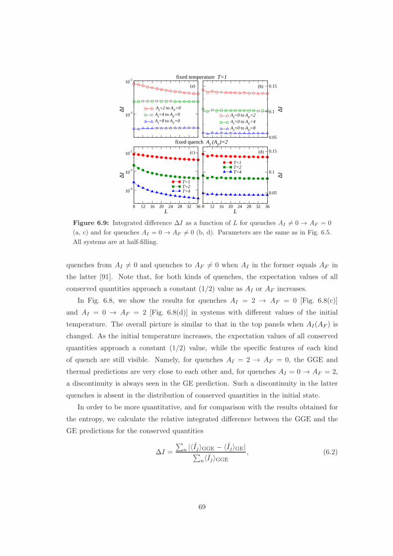
0.05

0.1

0.15

∆I

AI=0 to A

F=2

AI=0 to A

F=4

AI=0 to A

F=8

8 12 16 20 24 28 32 36L

10-4

10-3

10-2

∆I

T=1T=2T=4

10-3

10-2

∆I AI=2 to A

F=0

AI=4 to A

F=0

AI=8 to A

F=0

8 12 16 20 24 28 32 36L

0.05

0.1

0.15

∆I

T=1T=2T=4

(a) (b)

(c) (d)

fixed temperature T=1

fixed quench AI (A

F)=2

Figure 6.9: Integrated difference ∆I as a function of L for quenches AI 6= 0 → AF = 0

(a, c) and for quenches AI = 0 → AF 6= 0 (b, d). Parameters are the same as in Fig. 6.5.

All systems are at half-filling.

quenches from AI 6= 0 and quenches to AF 6= 0 when AI in the former equals AF in

the latter [91]. Note that, for both kinds of quenches, the expectation values of all

conserved quantities approach a constant (1/2) value as AI or AF increases.

In Fig. 6.8, we show the results for quenches AI = 2 → AF = 0 [Fig. 6.8(c)]

and AI = 0 → AF = 2 [Fig. 6.8(d)] in systems with different values of the initial

temperature. The overall picture is similar to that in the top panels when AI(AF ) is

changed. As the initial temperature increases, the expectation values of all conserved

quantities approach a constant (1/2) value, while the specific features of each kind

of quench are still visible. Namely, for quenches AI = 2 → AF = 0, the GGE and

thermal predictions are very close to each other and, for quenches AI = 0 → AF = 2,

a discontinuity is always seen in the GE prediction. Such a discontinuity in the latter

quenches is absent in the distribution of conserved quantities in the initial state.

In order to be more quantitative, and for comparison with the results obtained for

the entropy, we calculate the relative integrated difference between the GGE and the

GE predictions for the conserved quantities

∆I =

∑

n |〈Ij〉GGE − 〈Ij〉GE|∑

n〈Ij〉GGE

, (6.2)

69

1 10 100A

I , A

F

10-8

10-6

10-4

10-2

100

∆IT=1, A

I≠0 to A

F=0

T=2, AI≠0 to A

F=0

T=1, AI=0 to A

F≠0

T=2, AI=0 to A

F≠0

power-law fits

Figure 6.10: ∆I as a function of AI , for quenches AI 6= 0 → AF = 0 (open symbols), and

of AF , for quenches AI = 0 → AF 6= 0 (filled symbols), for two values of T . Dashed lines

depict power-law fits to the large AI (∆I ∼ 1/A3I) and AF (∆I ∼ 1/AI) results. Systems

are at half-filling with L = 32.

Scaling results for ∆I vs L are presented in Fig. 6.9. They are qualitatively similar to

those for the entropy differences in Fig. 6.5. In all quenches studied, the differences

between the GGE and the GE predictions for the entropies and the conserved quantities

are seen to saturate to a finite value with increasing system size. Also, the differences

between the GGE and the GE predictions for the conserved quantities decrease as

AI increases (for quenches AI 6= 0 → AF = 0) and as AF increases (for quenches

AI = 0 → AF 6= 0), as well as when T increases.

The dependence of ∆I on AI(AF ), for a fixed system size and for two different

temperatures, is depicted in Fig. 6.10. For both kinds of quenches, one can see that

∆I vanishes as a power law in the regime of large AI(AF ): for the quench from AI 6= 0

to AF = 0, ∆I decreases as ∆I ∼ 1/A3I , while for the opposite quench it decreases as

∆I ∼ 1/AF . One should note that, as expected from the discussion in Sec. 6.4, the

behavior seen for AI ≫ T is independent of T and identical to that in the ground state.

The exponents of the power laws are also independent of T for both quenches and are

found to be one-half those for (SGE − SGGE)/L vs AI(AF ).

∆I as a function of T is shown in Fig. 6.11, for three quenches AI 6= 0 → AF = 0

and for three quenches AI = 0 → AF 6= 0. The behavior of ∆I is once again similar to

that observed for (SGE − SGGE)/L vs T in the same quenches; ∆I vanishes as a power

law at very high temperatures. Power-law fits in the region T > 10 yield ∆I ∼ 1/T 3.04

70

1 5 10 20T

10-8

10-6

10-4

10-2

100

∆I AI=2 to A

F=0

AI=4 to A

F=0

AI=8 to A

F=0

AI=0 to A

F=2

AI=0 to A

F=4

AI=0 to A

F=8

power-law fits

Figure 6.11: ∆I as a function of T for quenches AI 6= 0 → AF = 0 (open symbols) and

quenches AI = 0 → AF 6= 0 (filled symbols). Dashed lines are power-law fits in the region

T > 10. We obtain ∆I ∼ 1/T 3.04 for quenches AI = 2 → AF = 0 and ∆I ∼ 1/T 1.00 for

quenches AI = 0 → AF = 2, respectively. All systems are at half-filling with L = 32.

for quenches AI = 2 → AF = 0 and ∆I ∼ 1/T 1.00 for quenches AI = 0 → AF = 2.

Once again, the exponents are found to be one-half those for (SGE − SGGE)/L vs T in

Sec. 6.4.

The preceding analysis clearly shows that only when the difference between the

conserved quantities in the initial state (in the GGE) and those in the thermal ensembles

becomes negligible do the entropies and the ensembles themselves become equivalent.

An understanding of this, as well as of the relation between the exponents of the power-

law decays seen for (SGE − SGGE)/L and ∆I, can be gained if one realizes that the

entropy in the GGE and the GE can be written in terms of the occupations of the

single-particle eigenstates as

S = −L∑

j=1

[(1 − Ij) ln(1− Ij) + Ij ln Ij], (6.3)

where Ij = 〈Ij〉GGE for the GGE and Ij = 〈Ij〉GE for the GE. Once the occupations

Ij in both ensembles are very close to each other, they are also very close to 1/2 (see

Fig. 6.8). One can write 〈Ij〉GE−1/2 = εGEj and 〈Ij〉GGE−1/2 = εGGE

j (with |εj | ≪ 1);

71

it is then straightforward to show that

SGE − SGGE =

L∑

j=1

{

2[

(εGGEj )2 − (εGE

j )2]

+4

3

[

(εGGEj )4 − (εGE

j )4]

+O[

(εGGEj )6 − (εGE

j )6]

}

, (6.4)

which provides an excellent description of the results for (SGE − SGGE)/L ≪ 1 in

Sec. 6.4 and decays with a power-law exponent that is twice that for ∆I.

72

7

Quench Dynamics of Chaotic

Initial States in Integrable

Systems

In this chapter, we study sudden quantum quenches in which the initial states are

selected to be either eigenstates of an integrable Hamiltonian that is nonmappable

to a noninteracting one or a nonintegrable Hamiltonian, while the Hamiltonian after

the quench is always integrable and mappable to a noninteracting one. By studying

weighted energy densities and entropies, we show that quenches starting from noninte-

grable (chaotic) eigenstates lead to an “ergodic” sampling of the eigenstates of the final

Hamiltonian, while those starting from the integrable eigenstates do not (or at least it

is not apparent for the system sizes accessible to us). This goes in parallel with the

fact that the distribution of conserved quantities in the initial states is thermal in the

nonintegrable cases and nonthermal in the integrable ones, and means that, in general,

thermalization occurs in integrable systems when the quench starts form an eigenstate

of a nonintegrable Hamiltonian (away from the edges of the spectrum), while it fails (or

requires larger system sizes than those studied here to become apparent) for quenches

starting at integrable points. We test those conclusions by studying the momentum

distribution function of HCBs after a quench.

73

7.1 Motivation

As discussed previously, the lack of thermalization of few-body observables of interest

in integrable systems has been attributed to the failure of the eigenstate thermalization

hypothesis (ETH). Hence, the outcome of the quench dynamics in such systems depends

on which eigenstates of the final Hamiltonian have a finite overlap with the initial

state. If the initial state samples the eigenstates within the microcanonical window

in an un-bias way, i.e., “ergodically,” then for that initial state the integrable system

will thermalize. This does not happen in most quenches between integrable systems

studied in the literature [45, 77–79, 82, 83, 86, 87, 89, 90, 94]. However, it has been

shown to occur for special initial states [91] with particular entanglement properties

[109], as well as for initial thermal states at infinite temperature (see Chap. 6) [112]. As

shown in Chap. 6, finite temperatures lead to a bias sampling of the final eigenstates

of the Hamiltonian after a quench.

In what follows, we discuss what happens in quenches from initial states that are

eigenstates of an integrable Hamiltonian that is nonmappable to a noninteracting one,

while the final Hamiltonian is integrable and mappable to a noninteracting one. This

is of interest as most studies in the literature have focused on quenches where both

the initial and final Hamiltonians are mappable to noninteracting ones. We also study

the case in which the initial state is an eigenstate of a nonintegrable Hamiltonian and

the final Hamiltonian is integrable. As argued in Ref. [107], initial states that are

eigenstates of nonintegrable Hamiltonians (away from the edges of the spectrum) can

lead to thermalization even though the final Hamiltonian is integrable. This can be

understood as the two-body interactions that break integrability in models of current

interest lead to quantum chaos even in the absence of randomness [113–116], similar to

what happens in systems with two-body random interactions [117–120]. As a result, the

eigenstates of nonintegrable Hamiltonians become random superpositions of eigenstates

of the integrable ones to which the quench is performed, i.e., they provide the unbiased

sampling required for thermalization after a quench to integrability. We do not find

indications that this happens in quenches between the integrable systems studied here.

74

7.2 Model Hamiltonian and Quench Protocol

We focus our study on 1D lattice HCBs in a box (a system with open boundary con-

ditions) with nearest-neighbor (NN) hopping t and interaction V , and next-nearest-

neighbor (NNN) hopping t′ and interaction V ′. The Hamiltonian reads

H=

L−1∑

i=1

−t(b†i bi+1 +H.c.) + V

(

ni −1

2

)(

ni+1 −1

2

)

+

L−2∑

i=1

−t′(b†i bi+2 +H.c.) + V ′

(

ni −1

2

)(

ni+2 −1

2

)

, (7.1)

with L the lattice size. In what follows, as in the previous chapter, the NN hopping

parameter sets the energy scale (t = 1), we take ~ = kB = 1 (where kB is the Boltzman

constant), and the number of particles N is selected to be N = L/3.

For t′ = V ′ = 0, Hamiltonian (7.1) is integrable (it can be mapped onto the spin-1/2

XXZ chain) [18]. For V 6= 0, it is nonmappable to a noninteracting model. However,

if V = 0, one can exactly solve Hamiltonian (7.1) by first mapping it onto the spin-1/2

XY chain through the Holstein-Primakoff transformation [34] and then onto noninter-

acting fermions by means of the Jordan-Wigner transformation [35], i.e., it is mappable

to a noninteracting model. Hence, the many-body eigenstates of the fermionic coun-

terpart are Slater determinants that can obtained from the single-particle Hamiltonian

without the need of diagonalizing the many-body one (see Chap. 2 for details). Prop-

erties of Slater determinants allow one to calculate off-diagonal correlations of HCBs

in polynomial time both in the many-body eigenstates of the Hamiltonian [36, 37, 71]

and in the grand-canonical ensemble [43]. The presence of nonzero NNN terms break

the integrability of the model and drive the system to a chaotic regime [113–116].

Here, we consider two types of quenches. Quench type I is within integrable models,

i.e, we keep t′ = V ′ = 0 at all times, and select the initial state to be an eigenstate

of Hamiltonian (7.1) with VI > 0, while the evolution is studied under Hamiltonian

(7.1) with VF = 0. Quench type II is from a nonintegrable model to an integrable

one: Namely, the initial state is selected to be an eigenstate of Hamiltonian (7.1) with

t′I = V ′I 6= 0 while the dynamics is studied under Hamiltonian (7.1) with t′F = V ′

F = 0.

In quench type II, we keep V = 0 at all times. Note that the final Hamiltonian in both

types of quenches is the same. One can fully diagonalize it for large systems by mapping

it onto noninteracting fermions as mentioned before. Since V 6= 0 and t′ = V ′ 6= 0 are

75

only present in the initial Hamiltonian, in what follows we drop the sub-index “I” from

VI and t′I = V ′I .

In order to compare results of quenches from eigenstates of different initial Hamil-

tonians, we select the initial states |ΨI〉 such that after the quench the systems have an

energy EI [Eq. (5.12)] which always corresponds to that of the canonical ensemble (CE)

at a fixed temperature TCE (the temperature is taken to be TCE ≈ 2 throughout this

work). The initial states, which are eigenstates of the t-V and t-t′-V ′ models, i.e., none

of which is mappable to a free model, are computed by means of the FILTLAN pack-

age that utilizes a polynomial filtered Lanczos procedure [121]. Since open boundary

conditions are imposed, the only remaining symmetry at 1/3 filling, and for V 6= 2, is

parity. Here, we restrict our analyses to the even parity sector, the dimension of which

is about 1/2 of the entire Hilbert space. The largest systems we study have L = 24,

whose total Hilbert space dimension is D =(248

)

= 735 471. The even parity subspace

for those systems has dimension Deven = 367 983. This is more than ten times larger

than the largest Hamiltonian sector diagonalized in previous full exact diagonalization

studies of similar systems [103, 104, 113–116]. In this work, the combination of utilizing

the Lanczos algorithm for computing the initial state, and full exact diagonalization

via the Bose-Fermi mapping for the final Hamiltonian, is what allows us to perform a

complete analysis for larger Hilbert spaces.

7.3 Overlaps

As mentioned before, in integrable systems, the lack of eigenstate thermalization im-

plies that the distribution of overlaps of the initial state with the eigenstates of final

Hamiltonian |Cα|2 plays a very important role in determining the expectation value of

observables after relaxation [Eq. (5.3)]. Therefore, we first study the values of |Cα|2 as

a function of Eα in quenches type I and type II and compare them to the weights of

the eigenstates of the final Hamiltonian in the CE, e−Eα/TCE/ZCE.

In Fig. 7.1, we show density plots of the coarse-grained values of |Cα|2 for different

type I quenches [Figs. 7.1(a)–7.1c)] and type II [Figs. 7.1(e)–7.1(h)]. The corresponding

results for the canonical weights (TCE ≈ 2) are presented in Figs. 7.1(d) and 7.1(h). One

can see in Fig. 7.1 that, for all values of V in quench type I and t′ = V ′ in quench type

II, the distribution of weights in the DE is qualitatively distinct from that in the CE,

76

-12

-8

-4

0

log 10

(Cα)

V=0.16

(a)0

1×104

2×104

3×104

t’=V’=0.08

(e)

-12

-8

-4

0

log 10

(Cα)

V=0.64

(b)0

1×104

2×104

3×104

t’=V’=0.32

(f)

-12

-8

-4

0

log 10

(Cα)

V=1.28

(c)0

1×104

2×104

3×104

t’=V’=1.28

(g)

-10 -5 0 5 10

Eα

-12

-8

-4

0

log 10

( e-E

α /T

CE/Z

CE ) TCE=2.006

(d)

-10 -5 0 5 10

Eα

0

0.5×106

1×106

1.5×106

TCE=1.989

(h)

Figure 7.1: Coarse-grained plot of the weights in the DE [(a)–(c) and (e)–(g)], and in the

CE [(d) and (h)], |Cα|2 and e−Eα/TCE/ZCE, respectively. (a)–(c) Results for quench type I

for different values of V . (e)–(g) Results for quench type II with different values of t′ = V ′.

(d) and (h) Weights in the CE, which correspond to effective temperatures TCE = 2.006

(EI = −4.976) and TCE = 1.989 (EI = −5.011), obtained for the quenches with V = 1.28

and t′ = V ′ = 1.28, respectively. All results are for L = 24, N = 8, and the temperatures

are TCE = 2.00± 0.01. The color scale indicates the number of states per unit area in the

plot.

which shows a simple exponential decay. In the diagonal ensemble, the weights between

eigenstates that are close in energy fluctuate wildly (note the logarithmic scale in the

y axes), and a maximum in the values of |Cα|2 [particularly clear in panels (a), (b), (e)

and (f)] can be seen around the energy of the initial state after the quench EI ≈ −5.0.

77

Hence, in contrast to the canonical ensemble, eigenstates of HF whose energies are close

to EI usually have the largest weights. This was also seen in Ref. [122].

Another feature that is apparent in Fig. 7.1 is that while the weights |Cα|2 decrease

rapidly as one moves away from EI , the number of states with those weights increases

dramatically for Eα > EI due to the increase of the density of states. For this reason,

the appropriate quantity to quantify how different regions of the spectrum contribute

to the observables in the diagonal ensemble (and in the CE) is the weighted energy

density function,

P (E) =1

∆E

∑

|E−Eα|<∆E/2

Wα, (7.2)

whereWα is |Cα|2 for the DE and e−Eα/TCE/ZCE for the CE. The summation is limited

to the states in a small energy window |E − Eα| < ∆E/2, the width of which (∆E) is

selected to be the same as for the coarse graining in Fig. 7.1. We have checked that

our results are robust for the selected values of ∆E.

The weighted energy density functions for the quenches studied in Fig. 7.1 are shown

in Fig. 7.2. There one can see that in all cases, except for the strongest quenches type

II, P (E) in the CE is much broader than that in the DE. For comparison, we have also

plotted the results for the energy shells, which are Gaussians (√2πδE)−1 exp[−(E −

EI)2/(2δE2)] with the same mean energy EI and energy width δE2 =

∑

α |Cα|2(Eα −EI)

2 as the diagonal ensemble. The energy shell has the maximal number of eigenstates

of the final Hamiltonian that is accessible to the particular initial state selected. In

quenches type I [Figs. 7.2(a)-7.2(c)], even for the largest V , P (E) in the diagonal

ensemble remains narrower than the energy shell. This is an indication of the lack

of “ergodicity” of the initial states associated with quench type I. On the contrary,

in quenches type II [Figs. 7.2(d)-7.2(f)], the width of P (E) in the diagonal ensemble

approaches that of the energy shell with increasing t′ = V ′. For the strongest quench

considered, t′ = V ′ = 1.281, P (E) in the DE and the CE become very close to each other

as well as to the energy shell [Fig. 7.2(f)]. The latter shows that initial states that are

1We are interested in understanding what happens in the thermodynamic limit for quenches that

may have arbitrarily large but finite [O(L0)] values of V or t′ = V

′. This ensures that the ratio

between the width of the weighted energy density distribution after the quench and the width of the

full energy spectrum vanishes in the thermodynamic limit [80]. Hence, here we are not concerned with

what happens for a finite system as V or t′ = V′ is increased to arbitrarily large values.

78

0

2

4

6

-8 -6 -4 -2 0P

(E)

V=0.16

(a) DECEenergy shellBWGaussian

0

1

2

3

4

-8 -6 -4 -2 0

t’=V’=0.08

(d)

0

0.2

0.4

0.6

-8 -6 -4 -2 0

t’=V’=0.32

(e)

0

1

2

3

4

-8 -6 -4 -2 0

P(E

)

V=0.64

(b)

0

0.4

0.8

1.2

1.6

-8 -6 -4 -2 0

P(E

)

E

V=1.28

(c)

0

0.05

0.1

0.15

0.2

-15 -10 -5 0 5 10

E

t’=V’=1.28

(f)

Figure 7.2: Weighted energy density functions P (E) for both the DE and the CE. (a)–(c)

Results for quenches type I. (e)–(f) Results for quenches type II. The dashed (blue) lines

depict the energy shell, where (a) EI = −4.99, δE = 0.159, (b) EI = −4.99, δE = 0.571,

(c) EI = −4.98, δE = 1.08, (d) EI = −5.00, δE = 0.253, (e) EI = −5.00, δE = 0.936,

and (f) EI = −5.01, δE = 2.66. Solid lines show the results of the fits of P (E) to the

most appropriate functional form. Thin lines are fits to a Breit-Wigner function with (a)

E = −5.01, Γ = 0.042, (b) E = −5.04, Γ = 0.101, (c) E = −5.17, Γ = 0.567, (d) E =

−4.99, Γ = 0.187, while thick lines are fits to a Gaussian with (e) E = −5.16, ∆ = 0.650,

and (f) E = −5.70, ∆ = 2.31. In all cases L = 24 and N = 8.

eigenstates of nonintegrable Hamiltonians sufficiently distant from an integrable point

fill the energy shell ergodically after a quench to integrability.

To better characterize P (E) as one goes from the weakest to the strongest quenches,

we have fitted it to two different functions: (i) a Breit-Wigner function,

P (E) =1

2π

Γ

(E − E)2 + (Γ/2)2, (7.3)

and (ii) a Gaussian,

P (E) =1√2π∆

exp

[−(E − E)2

2∆2

]

, (7.4)

where the mean energy E and half-width Γ of the Breit-Wigner function, as well as the

79

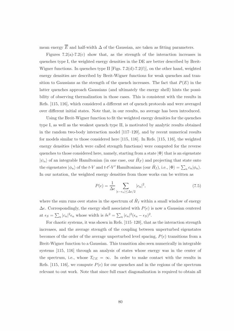
mean energy E and half-width ∆ of the Gaussian, are taken as fitting parameters.

Figures 7.2(a)-7.2(c) show that, as the strength of the interaction increases in

quenches type I, the weighted energy densities in the DE are better described by Breit-

Wigner functions. In quenches type II [Figs. 7.2(d)-7.2(f)], on the other hand, weighted

energy densities are described by Breit-Wigner functions for weak quenches and tran-

sition to Gaussians as the strength of the quench increases. The fact that P (E) in the

latter quenches approach Gaussians (and ultimately the energy shell) hints the possi-

bility of observing thermalization in those cases. This is consistent with the results in

Refs. [115, 116], which considered a different set of quench protocols and were averaged

over different initial states. Note that, in our results, no average has been introduced.

Using the Breit-Wigner function to fit the weighted energy densities for the quenches

type I, as well as the weakest quench type II, is motivated by analytic results obtained

in the random two-body interaction model [117–120], and by recent numerical results

for models similar to those considered here [115, 116]. In Refs. [115, 116], the weighted

energy densities (which were called strength functions) were computed for the reverse

quenches to those considered here, namely, starting from a state |Φ〉 that is an eigenstate

|ψα〉 of an integrable Hamiltonian (in one case, our HF ) and projecting that state onto

the eigenstates |φn〉 of the t-V and t-t′-V ′ Hamiltonians (our HI), i.e., |Φ〉 =∑

n cn|φn〉.In our notation, the weighted energy densities from those works can be written as

P (ǫ) =1

∆ǫ

∑

|ǫ−ǫn|≤∆ǫ/2

|cn|2, (7.5)

where the sum runs over states in the spectrum of HI within a small window of energy

∆ǫ. Correspondingly, the energy shell associated with P (ǫ) is now a Gaussian centered

at ǫS =∑

n |cn|2ǫn whose width is δǫ2 =∑

n |cn|2(ǫn − ǫS)2.

For chaotic systems, it was shown in Refs. [115–120], that as the interaction strength

increases, and the average strength of the coupling between unperturbed eigenstates

becomes of the order of the average unperturbed level spacing, P (ǫ) transitions from a

Breit-Wigner function to a Gaussian. This transition also seen numerically in integrable

systems [115, 116] through an analysis of states whose energy was in the center of

the spectrum, i.e., whose TCE = ∞. In order to make contact with the results in

Refs. [115, 116], we compute P (ǫ) for our quenches and in the regions of the spectrum

relevant to out work. Note that since full exact diagonalization is required to obtain all

80

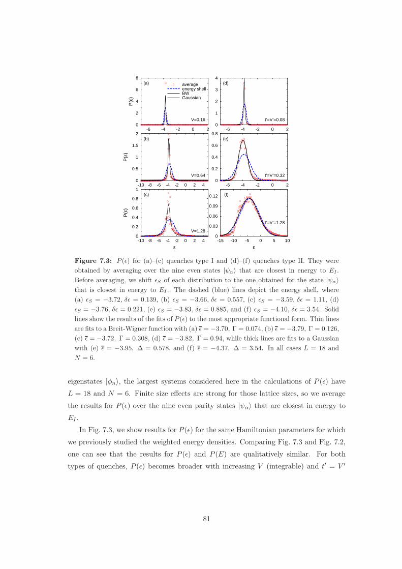
0

2

4

6

8

-6 -4 -2 0 2P

(ε)

V=0.16

(a) averageenergy shellBWGaussian

0

1

2

3

4

-6 -4 -2 0 2

t’=V’=0.08

(d)

0

0.2

0.4

0.6

0.8

-6 -4 -2 0 2

t’=V’=0.32

(e)

0

0.5

1

1.5

2

-10 -8 -6 -4 -2 0 2 4

P(ε

)

V=0.64

(b)

0

0.2

0.4

0.6

0.8

1

-10 -8 -6 -4 -2 0 2 4

P(ε

)

ε

V=1.28

(c)

0

0.03

0.06

0.09

0.12

-15 -10 -5 0 5 10

ε

t’=V’=1.28

(f)

Figure 7.3: P (ǫ) for (a)–(c) quenches type I and (d)–(f) quenches type II. They were

obtained by averaging over the nine even states |ψα〉 that are closest in energy to EI .

Before averaging, we shift ǫS of each distribution to the one obtained for the state |ψα〉that is closest in energy to EI . The dashed (blue) lines depict the energy shell, where

(a) ǫS = −3.72, δǫ = 0.139, (b) ǫS = −3.66, δǫ = 0.557, (c) ǫS = −3.59, δǫ = 1.11, (d)

ǫS = −3.76, δǫ = 0.221, (e) ǫS = −3.83, δǫ = 0.885, and (f) ǫS = −4.10, δǫ = 3.54. Solid

lines show the results of the fits of P (ǫ) to the most appropriate functional form. Thin lines

are fits to a Breit-Wigner function with (a) ǫ = −3.70, Γ = 0.074, (b) ǫ = −3.79, Γ = 0.126,

(c) ǫ = −3.72, Γ = 0.308, (d) ǫ = −3.82, Γ = 0.94, while thick lines are fits to a Gaussian

with (e) ǫ = −3.95, ∆ = 0.578, and (f) ǫ = −4.37, ∆ = 3.54. In all cases L = 18 and

N = 6.

eigenstates |φn〉, the largest systems considered here in the calculations of P (ǫ) have

L = 18 and N = 6. Finite size effects are strong for those lattice sizes, so we average

the results for P (ǫ) over the nine even parity states |ψα〉 that are closest in energy to

EI .

In Fig. 7.3, we show results for P (ǫ) for the same Hamiltonian parameters for which

we previously studied the weighted energy densities. Comparing Fig. 7.3 and Fig. 7.2,

one can see that the results for P (ǫ) and P (E) are qualitatively similar. For both

types of quenches, P (ǫ) becomes broader with increasing V (integrable) and t′ = V ′

81

(nonintegrable). However, when HI is integrable, P (ǫ) remains better described by

Breit-Wigner functions, while a transition from Breit-Wigner to Gaussian behavior, as

well as a filling of the energy shell [better seen in Fig. 7.3(f) than in Fig. 7.2(f)], is only

observed for a nonintegrable HI .

Our results for integrable systems are in contrast to those reported in Refs. [115,

116], where a transition from Breit-Wigner to Gaussian was also observed for an inter-

action quench within integrable systems. This can be attributed to the combination of

two effects. One is the fact that the states |ψα〉 selected here are far from the middle of

the spectrum, as was the case in Ref. [115, 116]. Within the entire spectrum, the mean

level spacing in the middle is the minimal one, i.e., the same perturbation may couple

more states in that region than away from it. If the average level spacing is the only

reason for the difference, then a transition should be seen in our case as one increases

the system size even further. This is a possibility that cannot be excluded within the

present study.

However, there may be another reason which would make the differences remain in

the thermodynamic limit. The result of averaging over eigenstates in the middle of the

spectrum [115, 116] leads to an ensemble at infinite temperature. In that ensemble, the

distribution of the quantities that are conserved after the quench could be featureless.

This would result in an un-bias sampling of the eigenstates of the Hamiltonian after

the quench, which may not occur for quenches starting at a finite temperature even if

they are strong quenches. We have found this to be the case in quenches in systems

with V = t′ = V ′ = 0 in which one starts from a thermal state [112]. Only the

initial state at infinite temperature was found to ergodically sample the eigenstates

after the quench, and a finite size scaling analysis showed that this does not change

with increasing system size (this was discussed in detail in the previous chapter). We

will come back to this point in Sec. 7.5, where the conserved quantities are studied for

all quenches considered here.

7.4 Entropies

The fact that the weighted energy density appears to be Gaussian after a quench to

integrability does not automatically guaranty that thermalization will occur, as it does

not mean that an un-bias sampling has been performed (unless the energy shell is filled).

82

One needs to keep in mind that a coarse-graining is involved when calculating P (E),

where ∆E [see Eq. (7.2)] is much larger than the average level spacing. For example,

in Ref. [112], we showed that quenches between integrable systems, which started from

thermal states, led to Gaussian like weighted energy distributions that are not thermal

and do not become thermal with increasing system size. The exception was the initial

infinite temperature state, which does lead to a thermal distribution after a quench

(but at infinite temperature). A qualitatively similar behavior was seen for quenches

starting from special pure states that are ground states of an integrable Hamiltonian

[91].

In order to quantify how the weights evolve in the DE as the system size increases,

10-3

10-2

10-1

100

S/L

L=15(a)

DEGGECEGE

10-1

100

L=15(e)

10-3

10-2

10-1

100

S/L

L=18(b) 10-1

100

L=18(f)

10-3

10-2

10-1

100

S/L

L=21(c) 10-1

100

L=21(g)

10-3

10-2

10-1

100

10-2 10-1 100

S/L

V

L=24(d) 10-1

100

10-2 10-1 100

t’=V’

L=24(h)

Figure 7.4: S/L for the DE, CE, GGE, and GE in systems with L = 15, 18, 21, and 24.

Results are presented for (a)–(d) quenches type I and (e)–(h) quenches type II.

83

and how they compare to the weights in the GGE, CE, and GE, we have computed

the entropies of the corresponding ensembles for all the quenches studied before. In

Fig. 7.4, we show all those entropies, per site, as a function of V for quenches type I

[Figs. 7.4(a)–7.4(d)] and of t′ = V ′ for quenches type II [Figs. 7.4(e)–7.4(h)], for four

system sizes. Since, in all cases, we consider a fixed effective temperature TCE ≈ 2 after

the quench, the values of S/L in the CE and the GE are (almost) independent of the

quench parameters.

The first feature that is apparent in Fig. 7.4 is that, in both types of quenches,

the entropy in the DE and the GGE are very small for weak quenches and increase

as system size increases. The GGE entropy follows (but is always above, as expected

from its grand-canonical nature) the DE entropy. In addition, for each quench, the dif-

ference between SDE, SGGE and SCE, SGE is seen to decrease with increasing system

size. However, only in quench type II one can see SGGE to become practically indistin-

guishable from SGE. If one agrees that the GGE describes observables after relaxation,

then the agreement between SGGE and SGE implies that the observables thermalize in

those quenches.

A better understanding of how the differences between entropies scale with in-

10-1

100

(SG

E-S

DE)/

L

(a)

L=15L=18L=21L=24 (c)

10-3

10-2

10-1

10-2 10-1 100

(SG

E-S

GG

E)/

L

V

(b)

10-2 10-1 100

t’=V’

(d)

Figure 7.5: (SGE − SDE)/L as a function of (a) V for quench type I and (c) t′ = V ′ for

quench type II. (SGE − SGGE)/L as a function of (b) V for quench type I and (d) t′ = V ′

for quench type II. Four different system sizes are presented for comparison.

84

creasing system size can be gained through Fig. 7.5. There we plot (SGE − SDE)/L

and (SGE − SGGE)/L for different system sizes. Since (SGE − SCE)/L vanishes in the

thermodynamic limit, we drop SCE from the remaining analysis. We note that the

analysis in Fig. 7.5 reflects small fluctuations in SGE (unnoticeable in Fig. 7.4) that

occur because EI is close but not identical

Figure 7.5 shows that, with increasing system size, a decrease of (SGE − SDE)/L

and a vanishing of (SGE − SGGE)/L is apparent only in quenches type II, which, once

again, indicates that thermalization will occur in those quenches. Furthermore, the

value of t′ = V ′ at which an abrupt reduction of the differences (SGE − SDE)/L and

(SGE − SGGE)/L occurs decreases as the system size increases, suggesting that in the

thermodynamic limit an infinitesimally small quench type II will lead to thermalization.

We should add that, in Fig. 7.5(d), the slight upturn (note the logarithmic scale in the

y axes) of (SGE − SGGE)/L for the strongest quenches is related to the skewing of the

weighted energy density seen in Fig. 7.2. Its effect is imperceptible in Fig. 7.5(c), as

(SGE−SDE)/L is more than an order of magnitude larger than (SGE−SGGE)/L. From

the evolution of the results with increasing size, we expect this upturn to disappear in

the thermodynamic limit. For quenches type I, the results in Figs. 7.5(a) and 7.5(b)

show that (SGE − SDE)/L and (SGE − SGGE)/L, respectively, either remain finite in

the thermodynamic limit or vanish very slowly with increasing system size. If the

latter were the case, larger system sizes are needed to conclusively see a decrease of

(SGE − SGGE)/L.

7.5 Conserved Quantities

As mentioned before, the presence of nontrivial sets of conserved quantities make inte-

grable systems different from nonintegrable ones. Hence, an understanding of whether

a particular initial state leads to thermalization can also be gained from analyzing how

the quantities that are conserved after the quench behave in the initial state. If the

distribution of conserved quantities is identical to the one in thermal equilibrium with

energy EI after the quench, then the initial state can provide an un-bias sampling of

the thermal one and lead to thermalization. Two particular examples in which that

happens, in quenches between integrable systems, were discussed in Refs. [91, 112].

85

0

0.2

0.4

0.6

0.8

1

⟨ Ij ⟩

V=0.04

(a)

GGEGE

t’=V’=0.04

(e)

0

0.2

0.4

0.6

0.8

1⟨ I

j ⟩

V=0.16

(b)

t’=V’=0.08

(f)

0

0.2

0.4

0.6

0.8

1

⟨ Ij ⟩

V=0.64

(c)

t’=V’=0.32

(g)

0

0.2

0.4

0.6

0.8

1

0 0.2 0.4 0.6 0.8 1

⟨ Ij ⟩

j/L

V=1.28

(d)

0 0.2 0.4 0.6 0.8 1

j/L

t’=V’=1.28

(h)

Figure 7.6: Distribution of conserved quantities 〈ΨI |Ij |ΨI〉 in the initial state (same as

the GGE) and in the GE. Results are presented for (a)–(d) quenches type I, and (e)–(h)

quenches type II. In all cases, L = 24 and N = 8.

However, in those examples, the distributions of conserved quantities were featureless

and corresponded to systems that were at infinite temperature after the quench.

In Fig. 7.6, we show the distribution of conserved quantities for various initial states

for quenches type I [Figs. 7.6(a)–7.6(d)] and type II [Figs. 7.6(e)–7.6(h)] in systems

with L = 24, and compare them to the distribution of conserved quantities in the GE

(which is almost identical in all quenches as EI is very close in all of them). That

figure shows that, in quenches type I, there are large differences between 〈ΨI |Ij |ΨI〉and the distribution of conserved quantities in the GE. In contrast, in quenches type II,

〈ΨI |Ij |ΨI〉 and the GE results approach each other and become very similar as t′ = V ′

increases.

86

10-1

100

10-2 10-1 100

∆I

V

(a)

L=15L=18L=21L=24

10-2 10-1 100

t’=V’

(b)

Figure 7.7: Relative integrated difference of the conserved quantities in the initial state

(in the GGE) and the GE, ∆I, as a function of (a) V for quench type I and (b) t′ = V ′

for quench type II. Results are presented for four system sizes.

In order to have a more quantitative understanding of the difference between the

conserved quantities in the initial state (in the GGE) and in the GE, as the system size

increases, we calculate the relative integrated difference ∆I defined in Eq. (6.2).

Results for ∆I in both types of quenches, and for different systems sizes, are pre-

sented in Fig. 7.7. They make evident that, as the system size increases in quenches

type II, the conserved quantities in the initial state converge to those predicted in ther-

mal equilibrium [as in Fig. 7.5(d), the upturn seen in Fig. 7.7(b) for large values of

t′ = V ′ is expected to disappear with increasing system size]. No such clear tendency

is seen for quenches type I. We note that the results for ∆I are qualitatively similar

to those obtained for (SGE − SGGE)/L in Fig. 7.5. As discussed in Chap. 6, this can

be understood as that the entropy in the GGE and in the GE can be written in terms

of the occupation of the single-particle eigenstates in each case, following the form in

Eqs. (6.3) and (6.4).

The results obtained for quenches type II imply that they will lead to thermalization

in integrable systems. This occurs even though the distribution of conserved quantities

is a nontrivial one (it is not flat, which was the case in Refs. [91, 112]). Beyond

its implication for the quantum dynamics of integrable systems, one could think of

using this information to learn about complicated many-body systems. It implies, e.g.,

that if we know the kinetic energy of a chaotic strongly correlated fermionic system in

equilibrium, we could automatically calculate its momentum distribution by computing

the momentum distribution function of a system that is in thermal equilibrium in

the noninteracting limit with the same energy as the kinetic energy of the strongly

87

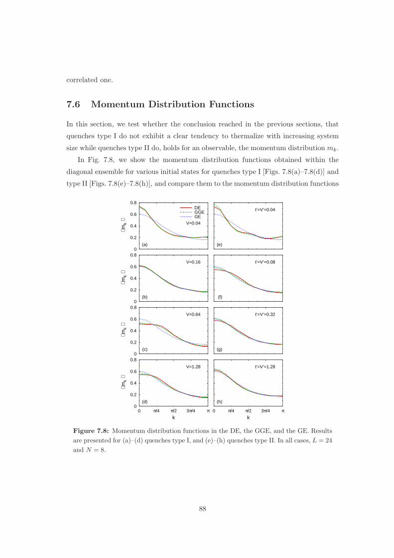
correlated one.

7.6 Momentum Distribution Functions

In this section, we test whether the conclusion reached in the previous sections, that

quenches type I do not exhibit a clear tendency to thermalize with increasing system

size while quenches type II do, holds for an observable, the momentum distribution mk.

In Fig. 7.8, we show the momentum distribution functions obtained within the

diagonal ensemble for various initial states for quenches type I [Figs. 7.8(a)–7.8(d)] and

type II [Figs. 7.8(e)–7.8(h)], and compare them to the momentum distribution functions

0

0.2

0.4

0.6

0.8

⟨ mk

⟩

V=0.04

(a)

DEGGEGE

t’=V’=0.04

(e)

0

0.2

0.4

0.6

0.8

⟨ mk

⟩

V=0.16

(b)

t’=V’=0.08

(f)

0

0.2

0.4

0.6

0.8

⟨ mk

⟩

V=0.64

(c)

t’=V’=0.32

(g)

0

0.2

0.4

0.6

0.8

0 π/4 π/2 3π/4 π

⟨ mk

⟩

k

V=1.28

(d)

0 π/4 π/2 3π/4 πk

t’=V’=1.28

(h)

Figure 7.8: Momentum distribution functions in the DE, the GGE, and the GE. Results

are presented for (a)–(d) quenches type I, and (e)–(h) quenches type II. In all cases, L = 24

and N = 8.

88

10-2

10-1

10-2 10-1 100

∆mD

E

V

(a)

10-2 10-1 100

t’=V’

(b)

L=15L=18L=21L=24

Figure 7.9: Relative integrated difference ∆mDE as a function of (a) V for quench type

I and (b) t′ = V ′ for quench type II. Results are presented for four system sizes.

predicted by the GGE and the GE1. That figure shows that while the GGE results

closely follow the ones in the DE for all quenches, the GE results are only consistently

closer to the DE ones as one increases t′ = V ′ in quenches type II [Figs. 7.8(f)–7.8(h)].

Once again, in order to be more quantitative, we compute the integrated differences

between the GE and DE results, namely

∆mDE =

∑

k |〈mk〉GE − 〈mk〉DE|∑

k〈mk〉GE. (7.6)

Results for ∆mDE are presented in Fig. 7.9(a) for quenches type I and in Fig. 7.9(b)

for quenches type II. In the former figure, no consistent trend is seen in the ∆mDE with

increasing system size. In contrast, in Fig. 7.9(b) one can see that, for the three largest

system sizes, ∆mDE decreases steadily with increasing L for t′ = V ′ between 0.1 and

1. For t′ = V ′ > 1, but finite, we expect that thermalization will also occur, with the

upturn seen in Fig. 7.9(b) for t′ = V ′ > 1 moving to larger values of t′ = V ′ as the

system size increases [107].

The results obtained for the momentum distribution functions are in agreement

with what was expected from our previous analysis, and indicates that quenches type

II lead to thermalization, while quenches type I do not lead to thermalization or require

much larger system sizes to observe an approach to the thermal predictions.

1We have also computed the momentum distribution functions within the CE. Those results, as

well as their differences with the ones obtained within the DE and the GGE, are not only qualitatively

but also quantitatively very similar to the ones discussed here for the GE. This is expected from the

finite size scaling analysis of this observable in the CE and the GE presented in Ref. [43].

89

8

Summary and Conclusions

In this thesis, we studied equilibrium and nonequilibrium properties of hard-core bosons

(HCBs) in one-dimensional optical lattices. We characterized various emerging phases

in equilibrium, as well as a delocalization to localization phase transition induced by

a quasi-periodic potential. We also studied the quench dynamics in isolated integrable

systems by systematically testing different classes of initial states.

In Chap. 2, we reviewed the main numerical approach used in this thesis to study

many-body properties of hard-core bosons. It is an exact method based on the mapping

between HCBs and noninteracting fermions. We showed that, by using the properties of

the Slater determinants, many-body correlation functions can be obtained diagonalizing

a single-particle Hamiltonian. Such a method made it possible for us to compute noise

correlations in very large systems.

In Chap. 3, by utilizing the exact approach introduced in Chap. 2, we conducted a

systematic study of the finite-size scaling of noise correlations in three different phases

that appear in homogeneous systems and in the presence of two different background

potentials. We showed that in the superfluid phase, the noise correlation peaks ∆00 ex-

hibit a leading linear behavior ∼L, independent of the filling factor and of the presence

of a superlattice potential. The subleading term was found to be strongly dependent on

the latter two. On the other hand, the fractional Mott and Bose-glass insulating phases

exhibit an asymptotic value that is independent of system size and only depends on

the filling factor and the strength of the potentials creating such phases. This behavior

is expected and manifests the absence of quasi-long-range order in these two phases.

90

In the period-two superlattice, we also found various peak-to-dip and dip-to-peak

transitions that were not observed in previous studies with smaller system sizes, some-

thing that demonstrates the importance of finite-size effects in the noise correlations

and the need for approaches that allow one to study very large system sizes. In the

disordered system (fractional Mott phase), we showed that the decrease of the ∆00

peak with increasing disorder strength (superlattice strength) exhibits a region with a

power-law decay ∆00 ∼ δ(V )−γ , with a nonuniversal value of exponent γ that depends

on the kind of perturbation creating the insulator.

In Chap. 4, we characterized the disorder-induced quantum phase transition be-

tween a superfluid and a Bose-glass phase in two-color incommensurate superlattices

by computing scaling exponents of the momentum distribution and noise correlation

peaks at k = 0. At the quantum phase transition, those observables, which are ac-

cessible in cold gases experiments, are found to scale with system size as ∼ N0.25 and

∼ N0.5, respectively. Intriguingly, the values of the exponents are one-half of their cor-

responding values in the superfluid phase, where the system is known to be described

by the Luttinger liquid theory with Luttinger parameter K = 1 [18]. We also showed

that, as expected, the scaling of those observables with system size vanishes in the

localized phase.

We also studied the behavior of momentum and noise correlation peaks, as well as

their first derivatives, as the superlattice strength is varied. We showed that both in

HCB and noninteracting spinless fermion systems the superfluid–Bose glass transition

is signaled by peaks in the first derivatives of the noise correlations. However, only in

the HCB case do those derivative peaks diverge with system size, providing a sharp

experimental signature of the phase transition.

In Chap. 5, we reviewed the framework to understand quantum quenches in isolated

systems. We introduced the statistical mechanics ensemble that is used to describe the

outcome of the quench dynamics in integrable systems, namely, the generalized Gibbs

ensemble (GGE), as well as the conventional thermal ensembles. We also discussed the

mechanism behind thermalization in generic (nonintegrable) systems as well as why

thermalization does not occur at integrability, and why the GGE works in that regime.

In Chap. 6, we studied properties of 1D lattice HCBs (XY chain) after quenches that

start from thermal initial states. In all cases considered, the quenches were generated

by sudden changes in a superlattice potential (a local space-dependent magnetic field

91

in the spin language). We showed that, in these integrable systems after a quench

starting from a finite-temperature state, the coarse-grained energy densities exhibit

a Gaussian shape. However, the distributions of the weights are still qualitatively

different between the quenched state and thermal states. This dissimilarity leads to an

extensive difference between the entropies in the isolated system after the quench (the

diagonal entropy), the GGE, and the thermal ensembles. On the other hand, as one

(or both) of the two control parameters explored here (the initial temperature T and

the strength of the superlattice AI or AF ) are tuned to infinity, all ensembles become

equivalent. The approach between the entropy of the GE and that of the GGE under

such tuning was shown to be power law in the control parameter, independent of the

quench protocol selected and of the values of the other parameters that were kept fixed.

It is important to emphasize that, when all parameters in the quenches were kept fixed

and finite and the system size was extrapolated to infinity, the differences between the

GGE and the GE results were seen to saturate at a finite value, i.e., these two ensembles

do not become equivalent.

We also showed that such differences have their origin in the disagreement between

the conserved quantities after the quench, which are determined by the initial state, and

the distribution of conserved quantities in thermal ensembles. By tuning the control

parameters mentioned above to infinity, we saw that the distribution of the conserved

quantities in the quenched state approaches that in thermal equilibrium, which ex-

plains why the generalized and thermal ensembles approach each other under those

conditions. However, we should stress that, in our particular systems of interest and

quench protocols followed, thermalization only occurs when the control parameters are

tuned to lead to completely flat distributions of conserved quantities, which is what

happens when the initial temperature is infinite or when AI(AF ) → ∞.

In Chap. 7, we studied quenches to an integrable Hamiltonian mappable to free

fermions, in which the initial state is selected to be either an eigenstate of an integrable

Hamiltonian that is nonmappable to a noninteracting one (quench type I) or an eigen-

state of a nonintegrable Hamiltonian (quench type II). By studying weighted energy

densities and entropies, we found no clear evidence that quenches type I, at least within

our Hamiltonians of interest and away from the middle of the spectrum, lead to an un-

bias sampling of the eigenstates of the final Hamiltonian. Quenches type II, on the

other hand, are found to provide such an un-bias sampling. Furthermore, an analysis

92

of different systems sizes indicates that, in the thermodynamic limit, an infinitesimal

quench type II will lead to thermalization. Here, an important requirement to keep in

mind is that the initial state must be away from the edges of the spectrum. This is

because, for systems with two-body interactions in the absence of randomness, chaotic

eigenstates can only be found away from the edges of the spectrum [113, 114].

We also showed that, in the initial state, an analysis of the distribution of the

quantities that are conserved after the quench provides an understanding of why ther-

malization occurs in one type of quenches while it fails in the other one. In quenches

type I, that distribution remains different from, or approaches very slowly with increas-

ing systems size, the one in thermal equilibrium after the quench. This implies that

an un-bias sampling of the eigenstates of the final Hamiltonian does not occur or takes

very large systems to be discerned. The opposite is true for quenches type II. Hence,

quenches type II provide a consistent way of creating initial states that have the ap-

propriate distribution of conserved quantities so that thermalization can occur after a

quench to integrability. Special initial states for which this occurred in quenches type

I were discussed in Refs. [91, 112]. However, the distribution of conserved quantities in

those cases was (trivially) flat corresponding to infinite temperature systems after the

quench.

Finally, by studying the momentum distribution functions in quenches type I and

type II, we showed that the conclusions reached on the basis of the results for the

energy distributions, entropies, and conserved quantities hold. Namely, we found no

indications that quenches type I lead to the thermalization of this observable while

quenches type II do result in thermal behavior.

93

Bibliography

[1] M. Anderson, J. Ensher, M. Matthews, C. Wieman, and E. Cornell. Observa-

tion of Bose-Einstein condensation in a dilute atomic vapor. Science, 269(5221):

198–201, 1995. 1, 2

[2] C. Raman, M. Kohl, R. Onofrio, D. S. Durfee, C. E. Kuklewicz, Z. Hadz-

ibabic, and W. Ketterle. Evidence for a critical velocity in a Bose-Einstein

condensed gas. Phys. Rev. Lett., 83: 2502–2505, Sep 1999. 2

[3] R. Onofrio, C. Raman, J. M. Vogels, J. R. Abo-Shaeer, A. P. Chikkatur, and

W. Ketterle. Observation of superfluid flow in a Bose-Einstein condensed gas.

Phys. Rev. Lett., 85: 2228–2231, Sep 2000. 2

[4] S. Burger, F. S. Cataliotti, C. Fort, F. Minardi, M. Inguscio, M. L. Chio-

falo, and M. P. Tosi. Superfluid and dissipative dynamics of a Bose-Einstein

condensate in a periodic optical potential. Phys. Rev. Lett., 86: 4447–4450, May

2001. 2

[5] F. S. Cataliotti, S. Burger, C. Fort, P. Maddaloni, F. Minardi, A. Trom-

bettoni, A. Smerzi, and M. Inguscio. Josephson junction arrays with Bose-

Einstein condensates. Science, 293(5531): 843–846, 2001. 2

[6] M. R. Matthews, B. P. Anderson, P. C. Haljan, D. S. Hall, C. E. Wieman,

and E. A. Cornell. Vortices in a Bose-Einstein condensate. Phys. Rev. Lett.,

83: 2498–2501, Sep 1999. 2

[7] K. W. Madison, F. Chevy, W. Wohlleben, and J. Dalibard. Vortex formation

in a stirred Bose-Einstein condensate. Phys. Rev. Lett., 84: 806–809, Jan 2000. 2

[8] J. R. Abo-Shaeer, C. Raman, J. M. Vogels, and W. Ketterle. Observation of

vortex lattices in Bose-Einstein condensates. Science, 292(5516): 476–479, 2001.

2

[9] P. C. Haljan, I. Coddington, P. Engels, and E. A. Cornell. Driving Bose-E-

instein-condensate vorticity with a rotating normal cloud. Phys. Rev. Lett., 87:

210403, Nov 2001. 2

94

[10] I. Bloch. Quantum coherence and entanglement with ultracold atoms in op-

tical lattices. Nature, 453(7198): 1016–1022, 2008. 3

[11] R. Grimm, M. Weidemuller, and Y. B. Ovchinnikov. Optical dipole traps for

neutral atoms. Advances in Atomic, Molecular, and Optical Physics, 42: 95–170, 2000.

2

[12] I. Bloch, J. Dalibard, and W. Zwerger. Many-body physics with ultracold

gases. Rev. Mod. Phys., 80: 885–964, Jul 2008. 5, 8

[13] M. Greiner, O. Mandel, T. Esslinger, T. Hansch, I. Bloch, et al. Quantum

phase transition from a superfluid to a Mott insulator in a gas of ultracold

atoms. Nature, 415(6867): 39–44, 2002. 7, 8, 35

[14] D. Jaksch, C. Bruder, J. Cirac, C. Gardiner, and P. Zoller. Cold bosonic

atoms in optical lattices. Phys. Rev. Lett., 81(15): 3108–3111, 1998. 7

[15] T. Stoferle, H. Moritz, C. Schori, M. Kohl, and T. Esslinger. Transition

from a strongly interacting 1d superfluid to a Mott insulator. Phys. Rev. Lett.,

92(13): 130403, Mar 2004. 7, 35

[16] I. B. Spielman, W. D. Phillips, and J. V. Porto. Mott-insulator transition in

a two-dimensional atomic Bose gas. Phys. Rev. Lett., 98(8): 080404, Feb 2007. 7

[17] I. B. Spielman, W. D. Phillips, and J. V. Porto. Condensate fraction in a

2D Bose gas measured across the Mott-insulator transition. Phys. Rev. Lett.,

100(12): 120402, Mar 2008. 7, 35

[18] M. A. Cazalilla, R. Citro, T. Giamarchi, E. Orignac, and M. Rigol. One

dimensional bosons: From condensed matter systems to ultracold gases. Rev.

Mod. Phys., 83: 1405–1466, Dec 2011. 8, 35, 37, 39, 75, 91

[19] T. Kinoshita, T. Wenger, and D. S. Weiss. Observation of a one-dimensional

Tonks-Girardeau gas. Science, 305(5687): 1125–1128, 2004. 8, 10, 35

[20] M. Greiner, I. Bloch, O. Mandel, T. Hansch, and T. Esslinger. Exploring

phase coherence in a 2D lattice of Bose-Einstein condensates. Phys. Rev. Lett.,

87(16): 160405, 2001. 8

[21] H. Moritz, T. Stoferle, M. Kohl, and T. Esslinger. Exciting collective oscil-

lations in a trapped 1D gas. Phys. Rev. Lett., 91: 250402, Dec 2003.

[22] B. Paredes, A. Widera, V. Murg, O. Mandel, S. Folling, I. Cirac, G. V.

Shlyapnikov, T. W. Hansch, and I. Bloch. Tonks-Girardeau gas of ultracold

atoms in an optical lattice. Nature, 429: 277–281, May 2004. 8, 10, 35

95

[23] I. Bloch. Ultracold quantum gases in optical lattices. Nature Physics, 1(1): 23–30,

2005. 9

[24] M. Girardeau. Relationship between systems of impenetrable bosons and

fermions in one dimension. J. Math. Phys., 1: 516–523, November 1960. 9

[25] E. Lieb, T. Schultz, and D. Mattis. Two soluble models of an antiferromag-

netic chain. Ann. Phys., 16(3): 406–466, 1961. 9, 15

[26] A. Lenard. Momentum distribution in the ground state of the one-dimensional

system of impenetrable bosons. J. Math. Phys., 5: 930, 1964. 10, 20, 23

[27] B. McCoy. Spin correlation functions of the XY model. Phys. Rev., 173(2): 531,

1968.

[28] H. Vaidya and C. Tracy. Crossover scaling function for the one-dimensional

XY model at zero temperature. Phys. Lett. A, 68(3-4): 378–380, 1978.

[29] H. Vaidya and C. Tracy. One-particle reduced density matrix of impenetrable

bosons in one dimension at zero temperature. Phys. Rev. Lett., 42(1): 3–6, 1979.

10

[30] M. Olshanii. Atomic scattering in the presence of an external confinement

and a gas of impenetrable bosons. Phys. Rev. Lett., 81: 938–941, Aug 1998. 10

[31] V. Dunjko, V. Lorent, and M. Olshanii. Bosons in cigar-shaped traps:

Thomas-Fermi regime, Tonks-Girardeau regime, and in between. Phys. Rev.

Lett., 86: 5413–5416, Jun 2001.

[32] D. S. Petrov, G. V. Shlyapnikov, and J. T. M. Walraven. Regimes of quantum

degeneracy in trapped 1D gases. Phys. Rev. Lett., 85: 3745–3749, Oct 2000. 10

[33] A. M. Rey, I. I. Satija, and C. W. Clark. Quantum coherence of hard-core

bosons: Extended, glassy, and Mott phases. Phys. Rev. A, 73(6): 063610, Jun

2006. 13, 14, 23, 35, 37, 41

[34] T. Holstein and H. Primakoff. Field dependence of the intrinsic domain

magnetization of a ferromagnet. Phys. Rev., 58(12): 1098–1113, Dec 1940. 14, 75

[35] P. Jordan and E. Wigner. About the Pauli exclusion principle. Z. Phys., 47:

631, 1928. 14, 75

[36] M. Rigol and A. Muramatsu. Universal properties of hard-core bosons con-

fined on one-dimensional lattices. Phys. Rev. A, 70(3): 031603(R), Sep 2004. 15,

17, 18, 20, 59, 75

96

[37] M. Rigol and A. Muramatsu. Ground-state properties of hard-core bosons

confined on one-dimensional optical lattices. Phys. Rev. A, 72(1): 013604, Jul

2005. 15, 17, 18, 20, 59, 75

[38] E. Altman, E. Demler, and M. D. Lukin. Probing many-body states of ultra-

cold atoms via noise correlations. Phys. Rev. A, 70(1): 013603, Jul 2004. 17, 21, 36,

38

[39] E. Toth, A. M. Rey, and P. B. Blakie. Theory of correlations between ul-

tracold bosons released from an optical lattice. Phys. Rev. A, 78: 013627, 2008.

17

[40] S. Folling, F. Gerbier, A. Widera, O. Mandel, T. Gericke, and I. Bloch.

Spatial quantum noise interferometry in expanding ultracold atom clouds.

Nature, 434(7032): 481–484, 2005. 20, 21, 22, 36, 38

[41] M. Girardeau, E. Wright, and J. Triscari. Ground-state properties of a one-

dimensional system of hard-core bosons in a harmonic trap. Phys. Rev. A, 63(3):

033601, 2001. 20

[42] G. Lapeyre, M. Girardeau, and E. Wright. Momentum distribution for a one-

dimensional trapped gas of hard-core bosons. Phys. Rev. A, 66(2): 23606–23606,

2002.

[43] M. Rigol. Finite-temperature properties of hard-core bosons confined on one-

dimensional optical lattices. Phys. Rev. A, 72(6): 063607, Dec 2005. 20, 51, 59, 75,

89

[44] V. G. Rousseau, D. P. Arovas, M. Rigol, F. Hebert, G. G. Batrouni, and

R. T. Scalettar. Exact study of the one-dimensional boson Hubbard model

with a superlattice potential. Phys. Rev. B, 73(17): 174516, May 2006. 20, 25, 36,

45

[45] M. Rigol, A. Muramatsu, and M. Olshanii. Hard-core bosons on optical su-

perlattices: Dynamics and relaxation in the superfluid and insulating regimes.

Phys. Rev. A, 74: 053616, Nov 2006. 20, 25, 26, 28, 47, 50, 51, 52, 74

[46] B. Horstmann, J. I. Cirac, and T. Roscilde. Dynamics of localization phe-

nomena for hard-core bosons in optical lattices. Phys. Rev. A, 76(4): 043625,

2007. 20

[47] M. Greiner, C. Regal, J. Stewart, and D. Jin. Probing pair-correlated

fermionic atoms through correlations in atom shot noise. Phys. Rev. Lett., 94(11):

110401, 2005. 22

97

[48] L. Mathey, A. Vishwanath, and E. Altman. Noise correlations in low-

dimensional systems of ultracold atoms. Phys. Rev. A, 79(1): 013609, Jan 2009.

23

[49] A. M. Rey, I. I. Satija, and C. W. Clark. Noise correlations of hard-core

bosons: quantum coherence and symmetry breaking. J. Phys. B, 39: S177, 2006.

26, 28, 33

[50] A. M. Rey, I. I. Satija, and C. W. Clark. Hanbury Brown-Twiss interferom-

etry for fractional and integer Mott phases. New J. Phys., 8(8): 155, 2006. 26,

28

[51] P. W. Anderson. Absence of diffusion in certain random lattices. Phys. Rev.,

109(5): 1492–1505, Mar 1958. 35

[52] F. Evers and A. D. Mirlin. Anderson transitions. Rev. Mod. Phys., 80(4): 1355–

1417, Oct 2008. 35

[53] J. Billy, V. Josse, Z. Zuo, A. Bernard, B. Hambrecht, P. Lugan, D. Clement,

L. Sanchez-Palencia, P. Bouyer, and A. Aspect. Direct observation of An-

derson localization of matter waves in a controlled disorder. Nature, 453(7197):

891–894, 2008. 35

[54] J. E. Lye, L. Fallani, M. Modugno, D. S. Wiersma, C. Fort, and M. Inguscio.

Bose-Einstein condensate in a random potential. Phys. Rev. Lett., 95(7): 070401,

2005. 35

[55] J. E. Lye, L. Fallani, C. Fort, V. Guarrera, M. Modugno, D. S. Wiersma,

and M. Inguscio. Effect of interactions on the localization of a Bose-Einstein

condensate in a quasiperiodic lattice. Phys. Rev. A, 75(6): 061603, 2007. 35

[56] L. Fallani, J. E. Lye, V. Guarrera, C. Fort, and M. Inguscio. Ultracold

atoms in a disordered crystal of light: towards a Bose glass. Phys. Rev. Lett.,

98(13): 130404, 2007.

[57] V. Guarrera, N. Fabbri, L. Fallani, C. Fort, K. M. R. van der Stam, and

M. Inguscio. Noise correlation spectroscopy of the broken order of a Mott

insulating phase. Phys. Rev. Lett., 100(25): 250403, 2008.

[58] G. Roati, C. D’Errico, L. Fallani, M. Fattori, C. Fort, M. Zaccanti,

G. Modugno, M. Modugno, and M. Inguscio. Anderson localization of a non-

interacting Bose-Einstein condensate. Nature, 453(7197): 895–898, 2008. 35

[59] T. Kinoshita, T. Wenger, and D. S. Weiss. Local pair correlations in one-

dimensional Bose gases. Phys. Rev. Lett., 95(19): 190406, Nov 2005. 35

98

[60] V. W. Scarola and S. Das Sarma. Cold-atom optical lattices as quantum

analog simulators for aperiodic one-dimensional localization without disorder.

Phys. Rev. A, 73(4): 041609, Apr 2006. 35

[61] S. Li, I. I. Satija, C. W. Clark, and A. M. Rey. Exploring complex phenomena

using ultracold atoms in bichromatic lattices. Phys. Rev. E, 82(1): 016217, Jul

2010. 36, 37, 42

[62] X. Cai, S. Chen, and Y. Wang. Superfluid-to-Bose-glass transition of hard-

core bosons in a one-dimensional incommensurate optical lattice. Phys. Rev.

A, 81(2): 023626, Feb 2010. 35

[63] R. Roth and K. Burnett. Phase diagram of bosonic atoms in two-color su-

perlattices. Phys. Rev. A, 68(2): 023604, 2003. 35

[64] P. Louis and M. Tsubota. Bosons in disordered optical potentials. J. Low Temp.

Phys., 148: 351–356, 2007. 35

[65] T. Roscilde. Bosons in one-dimensional incommensurate superlattices. Phys.

Rev. A, 77(6): 063605, 2008. 35, 37

[66] G. Roux, T. Barthel, I. P. McCulloch, C. Kollath, U. Schollwock, and

T. Giamarchi. Quasiperiodic Bose-Hubbard model and localization in one-

dimensional cold atomic gases. Phys. Rev. A, 78(2): 023628, 2008. 35

[67] X. Deng, R. Citro, A. Minguzzi, and E. Orignac. Phase diagram and momen-

tum distribution of an interacting Bose gas in a bichromatic lattice. Phys. Rev.

A, 78(1): 013625, 2008. 35

[68] J. B. Sokoloff. Unusual band structure, wave functions and electrical con-

ductance in crystals with incommensurate periodic potentials. Physics Reports,

126(4): 189–244, 1985. 36

[69] P. Buonsante, V. Penna, and A. Vezzani. Fractional-filling loophole insulator

domains for ultracold bosons in optical superlattices. Phys. Rev. A, 70: 061603,

Dec 2004. 36

[70] S. Aubry and G. Andre. Analyticity breaking and Anderson localization in

incommensurate lattices. Ann. Israel Phys. Soc., 3: 133, 1980. 37

[71] K. He and M. Rigol. Scaling of noise correlations in one-dimensional-lattice–

hard-core-boson systems. Phys. Rev. A, 83(2): 023611, Feb 2011. 39, 41, 59, 75

[72] M. Greiner, O. Mandel, T. Hansch, and I. Bloch. Collapse and revival of the

matter wave field of a Bose–Einstein condensate, 2002. Nature, 419: 51, 2002.

47

99

[73] T. Kinoshita, T. Wenger, and D. Weiss. A quantum Newton’s cradle. Nature,

440(7086): 900–903, 2006. 47

[74] S. Hofferberth, I. Lesanovsky, B. Fischer, T. Schumm, and J. Schmiedmayer.

Non-equilibrium coherence dynamics in one-dimensional Bose gases. Nature,

449(7160): 324–327, 2007.

[75] S. Will, T. Best, U. Schneider, L. Hackermuller, D.-S. Luhmann, and

I. Bloch. Time-resolved observation of coherent multi-body interactions in

quantum phase revivals. Nature, 465: 197–201, 2010.

[76] S. Trotzky, Y.-A. Chen, A. Flesch, I. P. McCulloch, U. Schollwock, J. Eis-

ert, and I. Bloch. Probing the relaxation towards equilibrium in an isolated

strongly correlated 1D Bose gas. Nature Phys., 8: 325, 2012. 47

[77] M. Rigol, V. Dunjko, V. Yurovsky, and M. Olshanii. Relaxation in a com-

pletely integrable many-body quantum system: An Ab Initio study of the

dynamics of the highly excited states of 1d lattice hard-core bosons. Phys. Rev.

Lett., 98(5): 050405, Feb 2007. 47, 48, 50, 51, 52, 53, 74

[78] M. A. Cazalilla. Effect of suddenly turning on interactions in the Luttinger

model. Phys. Rev. Lett., 97(15): 156403, Oct 2006.

[79] P. Calabrese and J. Cardy. Quantum quenches in extended systems. J. Stat.

Mech., page P06008, 2007. 74

[80] M. Rigol, V. Dunjko, and M. Olshanii. Thermalization and its mechanism for

generic isolated quantum systems. Nature, 452: 854, 2008. 53, 54, 78

[81] M. Eckstein and M. Kollar. Nonthermal steady states after an interaction

quench in the Falicov-Kimball model. Phys. Rev. Lett., 100(12): 120404, Mar 2008.

[82] M. Kollar and M. Eckstein. Relaxation of a one-dimensional Mott insulator

after an interaction quench. Phys. Rev. A, 78(1): 013626, Jul 2008. 50, 74

[83] A. Iucci and M. A. Cazalilla. Quantum quench dynamics of the Luttinger

model. Phys. Rev. A, 80(6): 063619, Dec 2009. 74

[84] D. Rossini, A. Silva, G. Mussardo, and G. E. Santoro. Effective thermal

dynamics following a quantum quench in a spin chain. Phys. Rev. Lett., 102(12):

127204, Mar 2009.

[85] D. Rossini, S. Suzuki, G. Mussardo, G. E. Santoro, and A. Silva. Long time

dynamics following a quench in an integrable quantum spin chain: Local ver-

sus nonlocal operators and effective thermal behavior. Phys. Rev. B, 82(14):

144302, Oct 2010.

100

[86] D. Fioretto and G. Mussardo. Quantum quenches in integrable field theories.

New J. Phys., 12: 055015, 2010. 74

[87] A. Iucci and M. A. Cazalilla. Quantum quench dynamics of the sine-Gordon

model in some solvable limits. New J. Phys., 12: 055019, 2010. 74

[88] J. Mossel and J.-S. Caux. Relaxation dynamics in the gapped XXZ spin-1/2

chain. New J. Phys., 12: 055028, 2010.

[89] A. C. Cassidy, C. W. Clark, and M. Rigol. Generalized thermalization in an

integrable lattice system. Phys. Rev. Lett., 106(14): 140405, Apr 2011. 50, 52, 55,

64, 74

[90] P. Calabrese, F. H. L. Essler, and M. Fagotti. Quantum quench in the

transverse-field Ising chain. Phys. Rev. Lett., 106(22): 227203, Jun 2011. 50, 74

[91] M. Rigol and M. Fitzpatrick. Initial-state dependence of the quench dynamics

in integrable quantum systems. Phys. Rev. A, 84: 033640, Sep 2011. 58, 62, 64, 66,

69, 74, 83, 85, 87, 93

[92] M. A. Cazalilla, A. Iucci, and M.-C. Chung. Thermalization and quantum

correlations in exactly solvable models. Phys. Rev. E, 85: 011133, Jan 2012.

[93] M. Kormos, A. Shashi, Y.-Z. Chou, and A. Imambekov. Interaction quenches

in the Lieb-Liniger model. arXiv:1204.3889, 2012. 47, 51

[94] P. Calabrese, F. H. L. Essler, and M. Fagotti. Quantum quenches in the

transverse field Ising chain: II. Stationary state properties. J. Stat. Mech.,

2012(07): P07022, 2012. 50, 74

[95] E. T. Jaynes. Information theory and statistical mechanics. Phys. Rev., 106(4):

620–630, May 1957. 51

[96] E. T. Jaynes. Information theory and statistical mechanics. II. Phys. Rev.,

108(2): 171–190, Oct 1957. 51

[97] M. Cramer, C. M. Dawson, J. Eisert, and T. J. Osborne. Exact relaxation

in a class of nonequilibrium quantum lattice systems. Phys. Rev. Lett., 100(3):

030602, Jan 2008. 51

[98] T. Barthel and U. Schollwock. Dephasing and the steady state in quantum

many-particle systems. Phys. Rev. Lett., 100(10): 100601, 2008. 51

[99] A. Polkovnikov. Microscopic diagonal entropy and its connection to basic

thermodynamic relations. Ann. Phys., 326(2): 486–499, 2011. 52

101

[100] L. F. Santos, A. Polkovnikov, and M. Rigol. Entropy of isolated quantum

systems after a quench. Phys. Rev. Lett., 107(4): 040601, 2011. 52, 63, 64

[101] J. Deutsch. Quantum statistical mechanics in a closed system. Phys. Rev. A,

43(4): 2046, 1991. 53

[102] M. Srednicki. Chaos and quantum thermalization. Phys. Rev. E, 50(2): 888,

1994. 53

[103] M. Rigol. Breakdown of thermalization in finite one-dimensional systems.

Phys. Rev. Lett., 103: 100403, Sep 2009. 53, 76

[104] M. Rigol. Quantum quenches and thermalization in one-dimensional fermionic

systems. Phys. Rev. A, 80: 053607, Nov 2009. 53, 76

[105] C. Gramsch and M. Rigol. Quenches in a quasidisordered integrable lattice

system: Dynamics and statistical description of observables after relaxations.

Phys. Rev. A, 86: 053615, 2012. 55

[106] K. He, L. F. Santos, T. M. Wright, and M. Rigol. Single-particle and

many-body analyses of a quasi-disordered integrable system after a quench.

arXiv:1304.2778, 2013. 55, 56

[107] M. Rigol and M. Srednicki. Alternatives to eigenstate thermalization. Phys.

Rev. Lett., 108: 110601, Mar 2012. 55, 74, 89

[108] S. Deng, G. Ortiz, and L. Viola. Dynamical critical scaling and effective

thermalization in quantum quenches: Role of the initial state. Phys. Rev. B,

83: 094304, Mar 2011. 58

[109] M.-C. Chung, A. Iucci, and M. A. Cazalilla. Thermalization in systems with

bipartite eigenmode entanglement. New Journal of Physics, 14(7): 075013, 2012.

58, 74

[110] K. He, I. I. Satija, C. W. Clark, A. M. Rey, and M. Rigol. Noise correlation

scalings: Revisiting the quantum phase transition in incommensurate lattices

with hard-core bosons. Phys. Rev. A, 85(1): 013617, 2012. 59

[111] M. Rigol and A. Muramatsu. Free expansion of impenetrable bosons on one-

dimensional optical lattices. Mod. Phys. Lett., 19: 861, 2005. 59

[112] K. He and M. Rigol. Initial-state dependence of the quench dynamics in

integrable quantum systems. II. Thermal states. Phys. Rev. A, 85: 063609, Jun

2012. 74, 82, 83, 85, 87, 93

102

[113] L. F. Santos and M. Rigol. Onset of quantum chaos in one-dimensional

bosonic and fermionic systems and its relation to thermalization. Phys. Rev. E,

81(3): 036206, 2010. 74, 75, 76, 93

[114] L. F. Santos and M. Rigol. Localization and the effects of symmetries in the

thermalization properties of one-dimensional quantum systems. Phys. Rev. E,

82: 031130, Sep 2010. 93

[115] L. F. Santos, F. Borgonovi, and F. M. Izrailev. Chaos and statistical relax-

ation in quantum systems of interacting particles. Phys. Rev. Lett., 108: 094102,

Mar 2012. 80, 82

[116] L. F. Santos, F. Borgonovi, and F. M. Izrailev. Onset of chaos and relaxation

in isolated systems of interacting spins: Energy shell approach. Phys. Rev. E,

85: 036209, Mar 2012. 74, 75, 76, 80, 82

[117] V. V. Flambaum, F. M. Izrailev, and G. Casati. Towards a statistical theory

of finite Fermi systems and compound states: Random two-body interaction

approach. Phys. Rev. E, 54: 2136–2139, Aug 1996. 74, 80

[118] V. V. Flambaum and F. M. Izrailev. Distribution of occupation numbers in

finite Fermi systems and role of interaction in chaos and thermalization. Phys.

Rev. E, 55: R13–R16, Jan 1997.

[119] V. V. Flambaum and F. M. Izrailev. Statistical theory of finite Fermi systems

based on the structure of chaotic eigenstates. Phys. Rev. E, 56: 5144–5159, Nov

1997.

[120] V. V. Flambaum and F. M. Izrailev. Excited eigenstates and strength func-

tions for isolated systems of interacting particles. Phys. Rev. E, 61: 2539–2542,

Mar 2000. 74, 80

[121] H. Fang and Y. Saad. A filtered lanczos procedure for extreme and interior

eigenvalue problems. SIAM Journal on Scientific Computing, 34(4): A2220–A2246,

2012. 76

[122] M. Rigol. Comment on “Quenches in quantum many-body systems: One-

dimensional Bose-Hubbard model reexamined”. Phys. Rev. A, 82(3): 037601,

Sep 2010. 78

103