Example 5.8

Non-logistics Network Models

5.1 | 5.2 | 5.3 | 5.4 | 5.5 | 5.6 | 5.7 | 5.9 | 5.10 | 5.10a

Background Information VanBuren Metals is a manufacturing company that

uses many large machines to work on metals.

These machines require frequent maintenance because of wear and tear, and VanBuren finds that it is sometimes advantageous, from a cost point of view, to replace machines rather than continue to maintain them.

For one particular class of machine, the company has estimated the quarterly cost of maintenance, the salvage value of reselling an old machine, and the cost of purchase a new machine.

5.1 | 5.2 | 5.3 | 5.4 | 5.5 | 5.6 | 5.7 | 5.9 | 5.10 | 5.10a

Background Information – continued We assume that the maintenance cost and the

salvage value depend on the age of the current machine, as well as the quarter in which they occur, whereas the purchase cost depends only on the quarter in which they occur, whereas the purchase cost depends only on the quarter in which it is purchased.

Essentially, maintenance costs increase with age and salvage values decrease with age, because of inflation.

5.1 | 5.2 | 5.3 | 5.4 | 5.5 | 5.6 | 5.7 | 5.9 | 5.10 | 5.10a

Background Information – continued VanBuren would like to devise a strategy for

purchasing machines over the next 5 years.

As a matter of policy, the company never sells a machine that is less than 1 year old, and it never keeps a machine that is more than 3 years old.

Also the machine in use at the beginning of the current quarter is brand new.

5.1 | 5.2 | 5.3 | 5.4 | 5.5 | 5.6 | 5.7 | 5.9 | 5.10 | 5.10a

Solution

The company’s first challenge is to estimate maintenance costs, salvage values, and purchase costs in the future months.

Although we could simply give these in a table and proceed directly to the optimization model, it is instructive to see how a company might actually estimate these monetary values from past data.

Presumably, the company owns several of these machines, and it has lots of historical data on maintenance, resales, and purchases.

5.1 | 5.2 | 5.3 | 5.4 | 5.5 | 5.6 | 5.7 | 5.9 | 5.10 | 5.10a

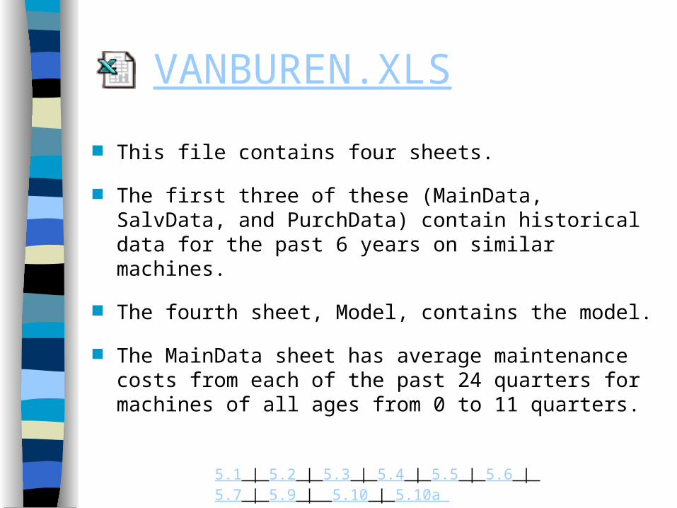
VANBUREN.XLS

This file contains four sheets.

The first three of these (MainData, SalvData, and PurchData) contain historical data for the past 6 years on similar machines.

The fourth sheet, Model, contains the model.

The MainData sheet has average maintenance costs from each of the past 24 quarters for machines of all ages from 0 to 11 quarters.

5.1 | 5.2 | 5.3 | 5.4 | 5.5 | 5.6 | 5.7 | 5.9 | 5.10 | 5.10a

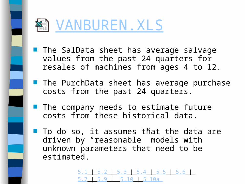
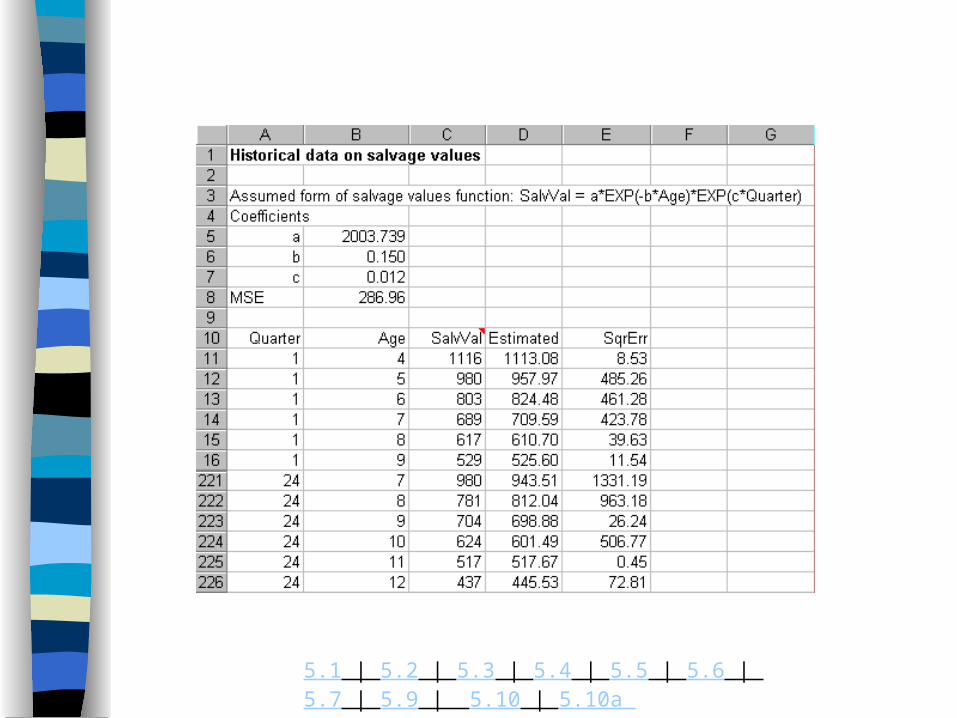
VANBUREN.XLS The SalData sheet has average salvage values from

the past 24 quarters for resales of machines from ages 4 to 12.

The PurchData sheet has average purchase costs from the past 24 quarters.

The company needs to estimate future costs from these historical data.

To do so, it assumes that the data are driven by “reasonable” models with unknown parameters that need to be estimated.

5.1 | 5.2 | 5.3 | 5.4 | 5.5 | 5.6 | 5.7 | 5.9 | 5.10 | 5.10a

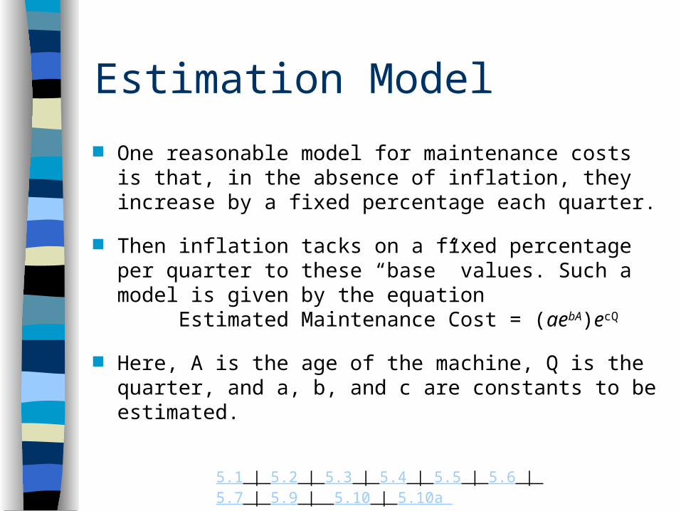
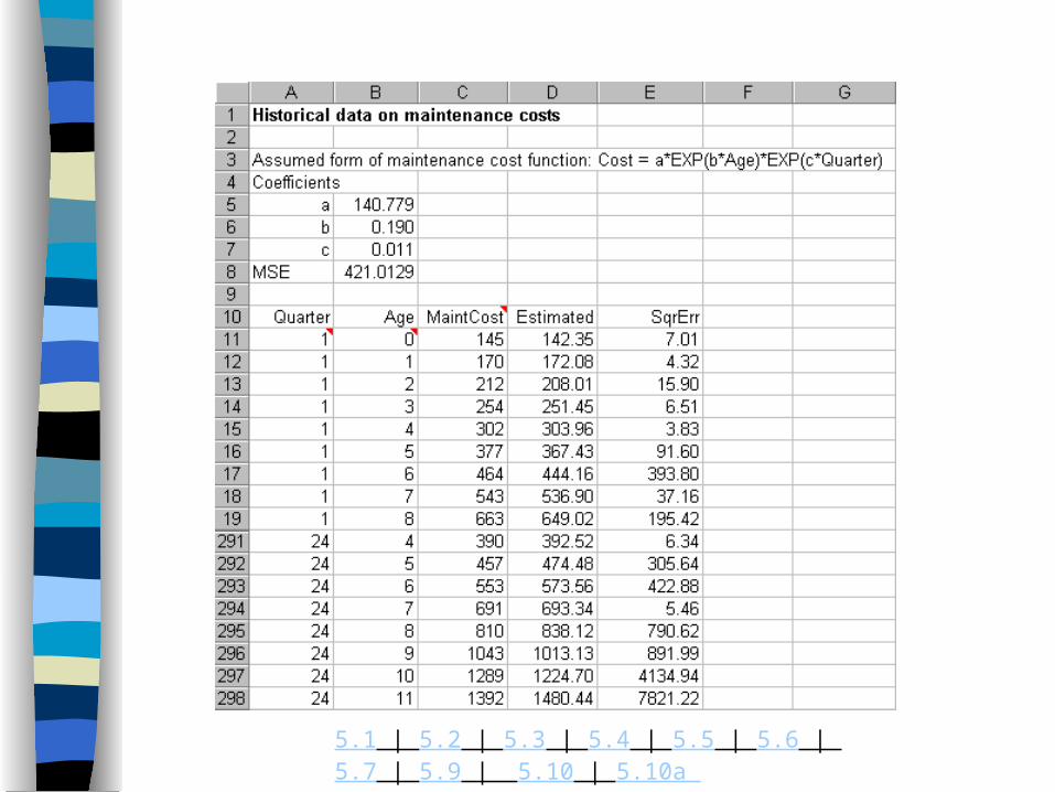
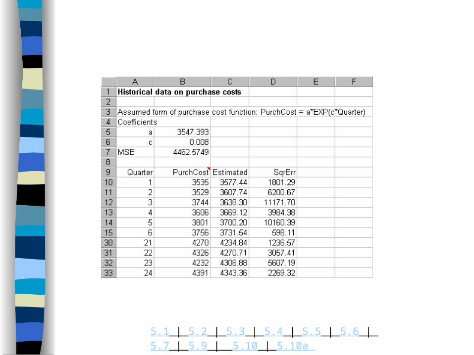
Estimation Model

One reasonable model for maintenance costs is that, in the absence of inflation, they increase by a fixed percentage each quarter.

Then inflation tacks on a fixed percentage per quarter to these “base” values. Such a model is given by the equation

Estimated Maintenance Cost = (aebA)ecQ

Here, A is the age of the machine, Q is the quarter, and a, b, and c are constants to be estimated.

5.1 | 5.2 | 5.3 | 5.4 | 5.5 | 5.6 | 5.7 | 5.9 | 5.10 | 5.10a

Estimation Model – continued We can interpret c as the percentage increase in

maintenance costs per extra quarter of age, and we can interpret c as the approximate inflation rate per quarter.

To estimate these constants, we can use Solver. The result is shown on the next slide.

The idea is to calculate estimated maintenance costs in column D, given trial values of the constants in the range B5:B7, calculate the squared differences between observed and estimated values in column E, average these squared errors in cell B8, and use Solver to minimize this “mean square error”(MSE).

5.1 | 5.2 | 5.3 | 5.4 | 5.5 | 5.6 | 5.7 | 5.9 | 5.10 | 5.10a

5.1 | 5.2 | 5.3 | 5.4 | 5.5 | 5.6 | 5.7 | 5.9 | 5.10 | 5.10a

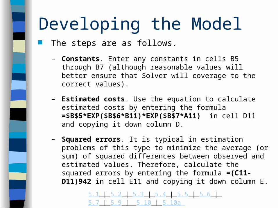
Developing the Model The steps are as follows.

– Constants. Enter any constants in cells B5 through B7 (although reasonable values will better ensure that Solver will coverage to the correct values).

– Estimated costs. Use the equation to calculate estimated costs by entering the formula =$B$5*EXP($B$6*B11)*EXP($B$7*A11) in cell D11 and copying it down column D.

– Squared errors. It is typical in estimation problems of this type to minimize the average (or sum) of squared differences between observed and estimated values. Therefore, calculate the squared errors by entering the formula =(C11-D11)942 in cell E11 and copying it down column E.

5.1 | 5.2 | 5.3 | 5.4 | 5.5 | 5.6 | 5.7 | 5.9 | 5.10 | 5.10a

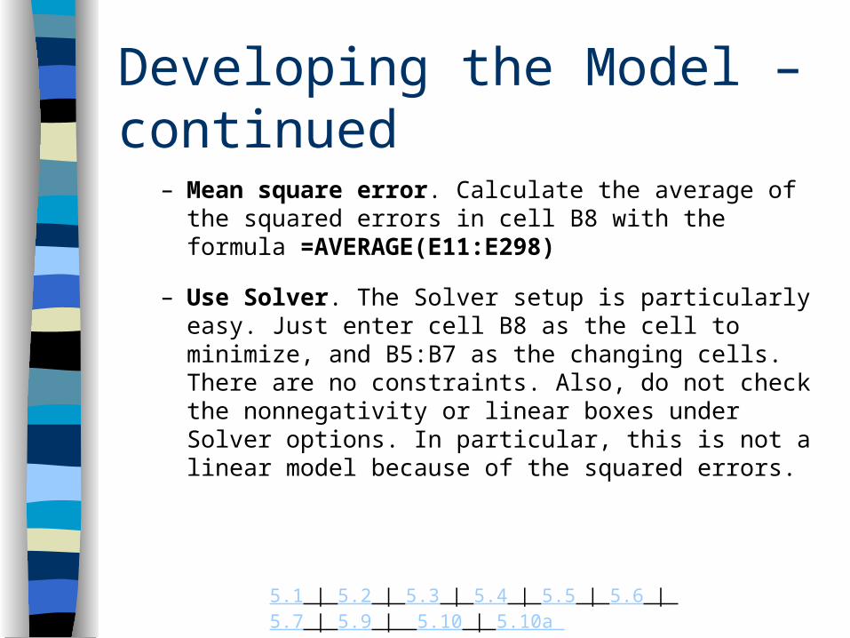
Developing the Model – continued

– Mean square error. Calculate the average of the squared errors in cell B8 with the formula =AVERAGE(E11:E298)

– Use Solver. The Solver setup is particularly easy. Just enter cell B8 as the cell to minimize, and B5:B7 as the changing cells. There are no constraints. Also, do not check the nonnegativity or linear boxes under Solver options. In particular, this is not a linear model because of the squared errors.

5.1 | 5.2 | 5.3 | 5.4 | 5.5 | 5.6 | 5.7 | 5.9 | 5.10 | 5.10a

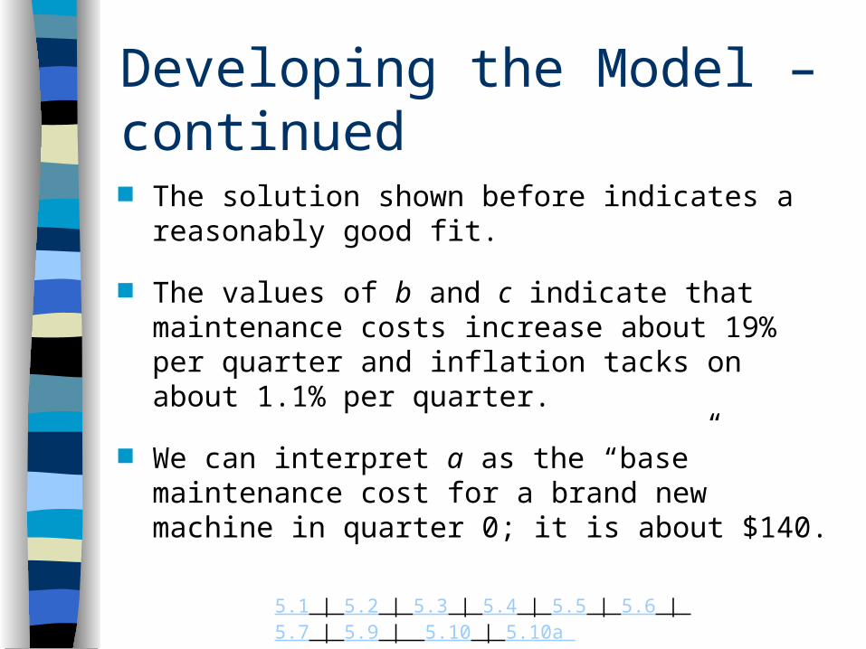
Developing the Model – continued The solution shown before indicates a reasonably

good fit.

The values of b and c indicate that maintenance costs increase about 19% per quarter and inflation tacks on about 1.1% per quarter.

We can interpret a as the “base” maintenance cost for a brand new machine in quarter 0; it is about $140.

5.1 | 5.2 | 5.3 | 5.4 | 5.5 | 5.6 | 5.7 | 5.9 | 5.10 | 5.10a

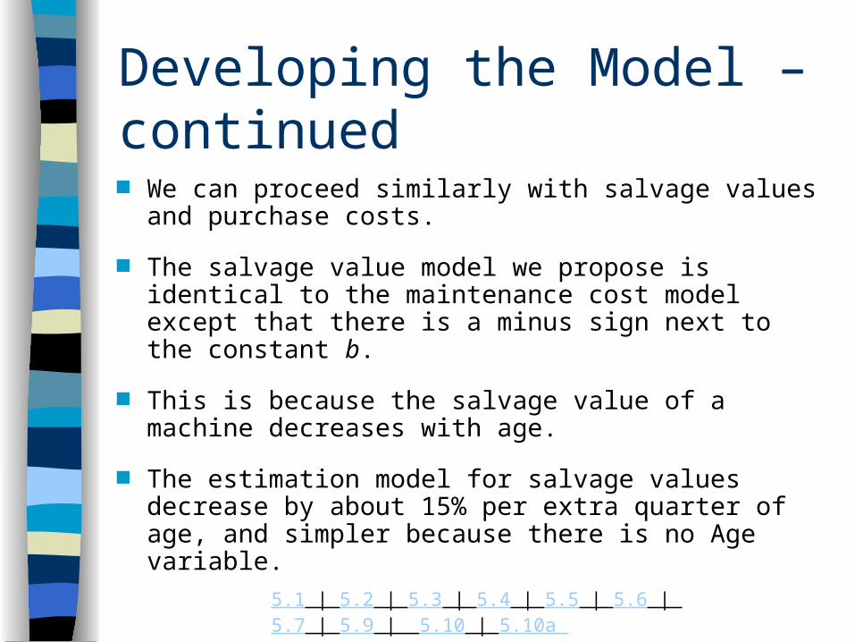
Developing the Model – continued We can proceed similarly with salvage values and

purchase costs.

The salvage value model we propose is identical to the maintenance cost model except that there is a minus sign next to the constant b.

This is because the salvage value of a machine decreases with age.

The estimation model for salvage values decrease by about 15% per extra quarter of age, and simpler because there is no Age variable.

5.1 | 5.2 | 5.3 | 5.4 | 5.5 | 5.6 | 5.7 | 5.9 | 5.10 | 5.10a

5.1 | 5.2 | 5.3 | 5.4 | 5.5 | 5.6 | 5.7 | 5.9 | 5.10 | 5.10a

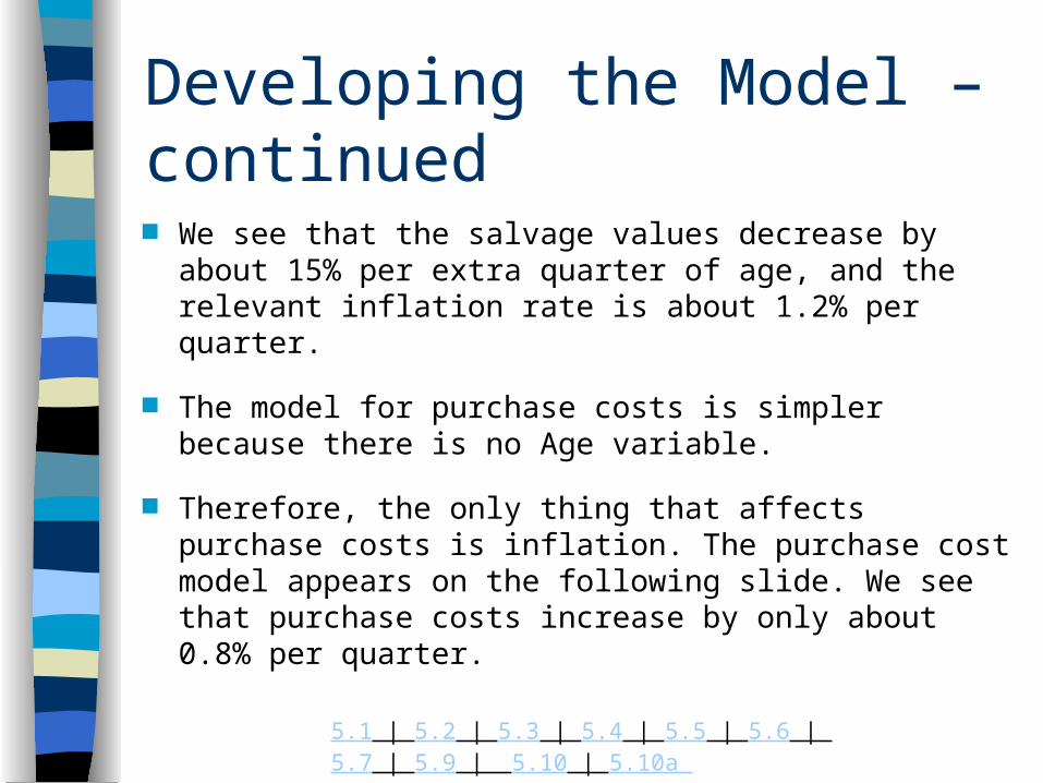
Developing the Model – continued We see that the salvage values decrease by about

15% per extra quarter of age, and the relevant inflation rate is about 1.2% per quarter.

The model for purchase costs is simpler because there is no Age variable.

Therefore, the only thing that affects purchase costs is inflation. The purchase cost model appears on the following slide. We see that purchase costs increase by only about 0.8% per quarter.

5.1 | 5.2 | 5.3 | 5.4 | 5.5 | 5.6 | 5.7 | 5.9 | 5.10 | 5.10a

5.1 | 5.2 | 5.3 | 5.4 | 5.5 | 5.6 | 5.7 | 5.9 | 5.10 | 5.10a

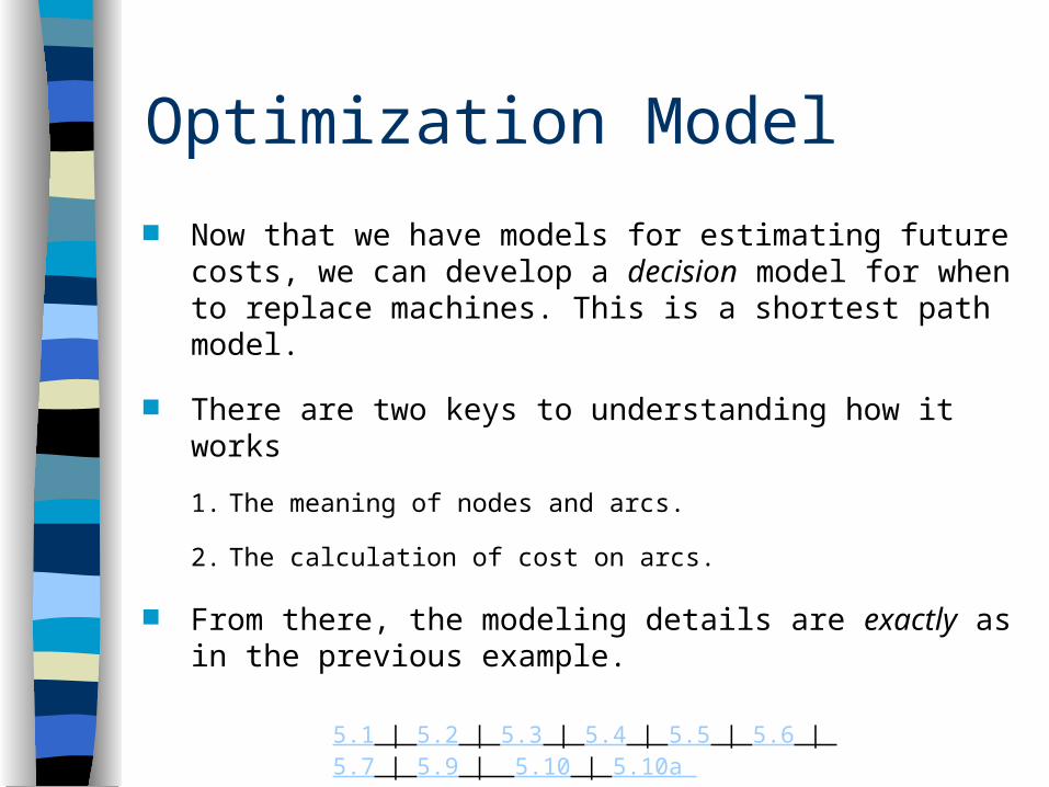
Optimization Model

Now that we have models for estimating future costs, we can develop a decision model for when to replace machines. This is a shortest path model.

There are two keys to understanding how it works

1. The meaning of nodes and arcs.

2. The calculation of cost on arcs.

From there, the modeling details are exactly as in the previous example.

5.1 | 5.2 | 5.3 | 5.4 | 5.5 | 5.6 | 5.7 | 5.9 | 5.10 | 5.10a

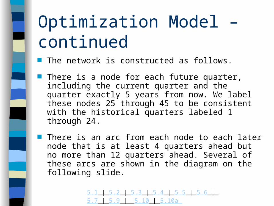
Optimization Model – continued

The network is constructed as follows.

There is a node for each future quarter, including the current quarter and the quarter exactly 5 years from now. We label these nodes 25 through 45 to be consistent with the historical quarters labeled 1 through 24.

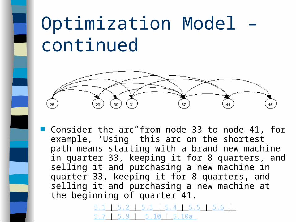
There is an arc from each node to each later node that is at least 4 quarters ahead but no more than 12 quarters ahead. Several of these arcs are shown in the diagram on the following slide.

5.1 | 5.2 | 5.3 | 5.4 | 5.5 | 5.6 | 5.7 | 5.9 | 5.10 | 5.10a

Optimization Model – continued

Consider the arc from node 33 to node 41, for example, ‘Using” this arc on the shortest path means starting with a brand new machine in quarter 33, keeping it for 8 quarters, and selling it and purchasing a new machine in quarter 33, keeping it for 8 quarters, and selling it and purchasing a new machine at the beginning of quarter 41.

5.1 | 5.2 | 5.3 | 5.4 | 5.5 | 5.6 | 5.7 | 5.9 | 5.10 | 5.10a

Optimization Model – continued

An entire strategy for the 5-year period is a string of such arcs.

For example, if the shortest path is 25-33-41-45, then VanBuren keeps the first machine for 8 quarters, purchases a third machine in quarter 41, keeps it for 4 quarters, and finally trades it in for a new machine in quarter 45.

Given the meaning the arcs, the calculation of arc costs is a matter of careful bookkeeping.

5.1 | 5.2 | 5.3 | 5.4 | 5.5 | 5.6 | 5.7 | 5.9 | 5.10 | 5.10a

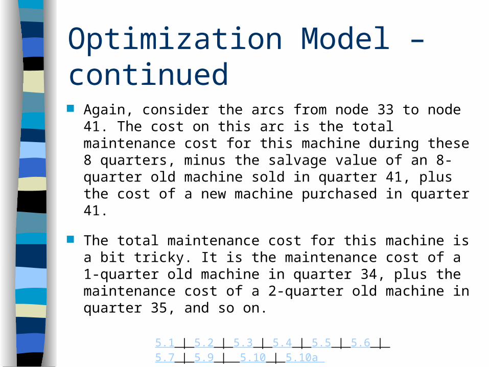
Optimization Model – continued

Again, consider the arcs from node 33 to node 41. The cost on this arc is the total maintenance cost for this machine during these 8 quarters, minus the salvage value of an 8-quarter old machine sold in quarter 41, plus the cost of a new machine purchased in quarter 41.

The total maintenance cost for this machine is a bit tricky. It is the maintenance cost of a 1-quarter old machine in quarter 34, plus the maintenance cost of a 2-quarter old machine in quarter 35, and so on.

5.1 | 5.2 | 5.3 | 5.4 | 5.5 | 5.6 | 5.7 | 5.9 | 5.10 | 5.10a

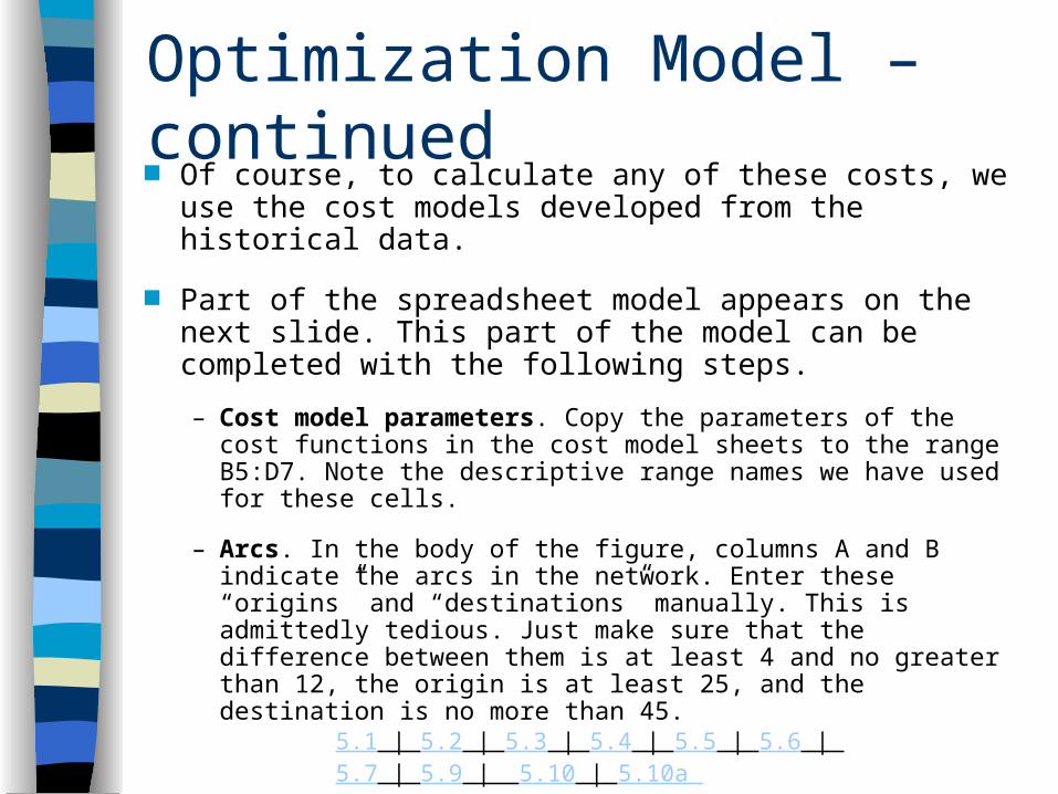
Optimization Model – continued Of course, to calculate any of these costs, we use the

cost models developed from the historical data.

Part of the spreadsheet model appears on the next slide. This part of the model can be completed with the following steps.

– Cost model parameters. Copy the parameters of the cost functions in the cost model sheets to the range B5:D7. Note the descriptive range names we have used for these cells.

– Arcs. In the body of the figure, columns A and B indicate the arcs in the network. Enter these “origins” and “destinations” manually. This is admittedly tedious. Just make sure that the difference between them is at least 4 and no greater than 12, the origin is at least 25, and the destination is no more than 45.

5.1 | 5.2 | 5.3 | 5.4 | 5.5 | 5.6 | 5.7 | 5.9 | 5.10 | 5.10a

5.1 | 5.2 | 5.3 | 5.4 | 5.5 | 5.6 | 5.7 | 5.9 | 5.10 | 5.10a

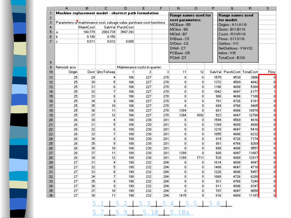
Optimization Model – continued

– Differences. Calculate the differences between the values in columns B and A in column C. These differences indicate how many quarters the machine is kept for each arc.

– Maintenance costs. Calculate the quarterly maintenance costs in columns D through O. For example, for the arc from 25 to 29 in row 11, cell D11 contains the maintenance cost in the first quarter of this period, cell E11 contains the maintenance cost in the second quarter of this period, and so on. Fortunately, you can calculate all of these maintenance costs at once by entering the formula =IF(D$10<=$C11,MCBase*EXP(MCIncr*(D$10-1))*EXP(MCInfl*($A11+D$10-1)),0) in cell D11 and copying it to the range D11:O118.

5.1 | 5.2 | 5.3 | 5.4 | 5.5 | 5.6 | 5.7 | 5.9 | 5.10 | 5.10a

Optimization Model – continued

– The IF Function is used to ensure that no maintenance costs for this machine are incurred unless it is still owned. The rest of this rather complex formula is the Excel implementation of the equation.

– Salvage values and purchase costs. In a similar way, calculate the salvage values in column P by entering the formula =SVBase*EXP(-SVDecr*$C11)*EXP(SVInfl*($B11)) in cell P11 and copying down column P. Then calculate the purchase costs in column Q by entering the formula =PCBase*EXP(PCInfl*($B11)) in cell Q11 and copying down column Q.

5.1 | 5.2 | 5.3 | 5.4 | 5.5 | 5.6 | 5.7 | 5.9 | 5.10 | 5.10a

Optimization Model – continued– Total arc costs. Calculate the total costs on the arcs as

total maintenance cost minus salvage value plus purchase cost. To do this, enter the formula =SUM(D11:O11)-P11+Q11 in cell R11, and copy it down column R.

– Flows. Enter any flows on the arcs in column S.

From this point, the model is developed exactly as in the shortest path model of Example 5.7, with node 25 as the “origin” node and node 45 as the “destination” node.

We create the flow balance constraints, calculate the total network cost, and use Solver exactly as before, so we won’t repeat the details here.

5.1 | 5.2 | 5.3 | 5.4 | 5.5 | 5.6 | 5.7 | 5.9 | 5.10 | 5.10a

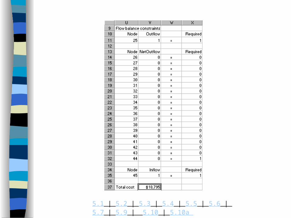
Optimization Model – continued The constraints and objective for machine

replacement model is shown on the next slide.

Also, we find the shortest path, we follow the 1’s in the Flows range.

You can check the VANBUREN.XLS file that only three arcs have flows of 1: 25-32, 32-39, and 39-45.

Therefore, VanBuren should keep the current machine for 7 quarters, resell it and buy a new machine in quarter 32, keep the second machine for 7 quarters, resell it and buy a new machine in quarter 39, keep it for 6 quarters, and finally resell it and buy a new machine in quarter 45.

The total cost of this strategy is $18,795.

5.1 | 5.2 | 5.3 | 5.4 | 5.5 | 5.6 | 5.7 | 5.9 | 5.10 | 5.10a