excel 2016 basics for windows - myusf · excel 2016 basics for windows training objective to learn...

1

The Center for Instruction and Technology Last updated: 9/28/16

Excel 2016 Basics for Windows

Excel 2016 Basics for Windows Training Objective

To learn the tools and features to get started using Excel 2016 more efficiently and effectively.

What you can expect to learn from this class:

How to approach the Excel interface

How to use the tools available in Excel

How to edit cells and move around

How to use and customize Excel’s toolbar

Excel’s many mouse-oriented tools

How to use the right-mouse button

How to create formulas

How to cut, copy and paste

Understand the difference between values and formulas in Excel

How to use Excel’s functions

How to use some of Excel’s helpful features: AutoFill, Notes, and Autoformat.

How to format an Excel worksheet

How to develop a page setup and printing

Who should take this class?

Any person who wants to learn how to use Excel 2016 to create dynamic worksheets, forms and spreadsheets.

Excel Tips and Shortcuts:

Always press Enter to close a cell Control-Z to Undo. Control-S to perform frequent Quick Saves. Control-Home to go to the top of worksheet Control-C to Copy Control-X to Cut Control-V to Paste Control-A to Select All Double-click to Edit a cell Shift-click to select a range of cells Control-click to select a non-consecutive range of cells Right-click to access a Quick Menu

2


Getting Started

Before creating a worksheet consider how the worksheet will be used and how it will look. 1. Begin by creating a sample worksheet on paper. 2. Think through your objective. 3. Consider who will use it. 4. Consider what type of input is required.

Steps for developing an Excel Worksheet 1. Create Labels (column and row headings) 2. Add numbers 3. Add formulas 4. Format the worksheet

Getting Started-The New Look of Office 2016 Before we begin looking at the functions we need to introduce the new interface of Excel 2016.

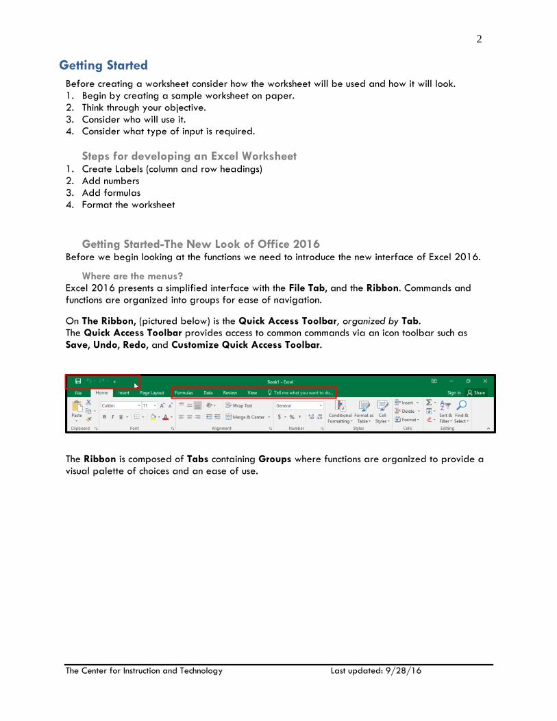
Where are the menus? Excel 2016 presents a simplified interface with the File Tab, and the Ribbon. Commands and functions are organized into groups for ease of navigation.

On The Ribbon, (pictured below) is the Quick Access Toolbar, organized by Tab. The Quick Access Toolbar provides access to common commands via an icon toolbar such as

Save, Undo, Redo, and Customize Quick Access Toolbar.

The Ribbon is composed of Tabs containing Groups where functions are organized to provide a visual palette of choices and an ease of use.

3


The 3 buttons in the bottom right corner of the document window allow you to change the way you view your document. Also in this area is the Zoom tool to allow you to enlarge the view of the document for a closer look. NOTE: you can also choose these options from the View Tab > from the Workbook Views Group on the Ribbon.

Normal View is the default.

Page Layout View can be used when you want to view the page as if it were in Print Preview mode. Use Page Layout to see where pages begin and end and to view any headers or footers on the page.

Page Break Preview is used to view where pages will break when the document is printed and also to maximize the space available for reading or commenting on the document.

Online Help Use the Microsoft Office Excel Tell Me dialog box for quick answers to Excel 2016 questions. Click twice in the upper right corner of the Ribbon and type in a question.

Saving Save versus Save As: use Save to save a previously saved document; use Save As to save a new document or to save another copy of the document under a different name or format.

1. Select Save As from the File tab. 2. When the Save As dialog box appears, type in a name for the file in the File Name text

boxes. If you need to change the format of a document for someone who isn’t using Excel 2016, select Excel 97-2003 in the Save as type drop down menu to save the document in a previous version of Excel.

3. Choose a destination for the file to be saved. 4. Click Save to save the file.

4


Save: Click once on the Disk icon (or Control-S) in the Quick Access Toolbar to perform a quick save.

The Open File Dialog Quickly open any previous documents used by selecting them from the Recent Documents pane when you click on File Tab menu. You can also choose Open from the File Tab. Tip: Change the Recent Documents setting from Excel Options in the File Tab menu. Select Advanced, and in the Display section, increase or decrease the number in Show this number of Recent Documents up to 50 documents.

5


The Excel Window The Excel window consists of a series of bars, columns and rows, and their intersection: cells.

Excel’s Bars Title Bar is the first bar in the worksheet and identifies the workbook name. The Tool Bar

consists of icons which allow you easy access to

The Formula Bar contains the active cell location to the left, and the cell contents to the right

The Sheet Tabs Bar contains worksheets within a workbook. Double-click on a tab to rename it. Tip: right-click over a sheet and choose Move or Copy Sheet from the Edit menu to copy a finished sheet. Make sure you check the Create a Copy checkbox if you want to create a copy of a worksheet.

The Status Bar displays the command functions and keyboard toggles.

Vertical and Horizontal scroll bars are located on the edges of the worksheet. Use your mouse and the arrow keys to move through the worksheet.

Split bars are used to separate windows into panes for locking titles. They are small gray rectangles located at the top of the vertical bar and to the far right of the horizontal bar.

Cells The Excel worksheet is divided out into cells, separated by horizontal and vertical gridlines. Cells are the basic unit of a worksheet, used to store text, values, formulas and functions.

File Tab Menu

Status Bar

Formula Bar Title Bar

Sheet Tabs Bar

Split Bar

Active Cell

6


Misc.

The Active Cell is the cell surrounded by bold borders.

Column headings range from A through IV; Row Headings are labeled from 1 through 65,536. Select the View tab in the Ribbon and choose from the options in the Window group to view more than one worksheet at a time.

Setting Your Default Directory To change the default directory, select Excel Options from the File Tab; then select from the Save category and change the Default File Location to the desired directory.

Moving around the Worksheet Use the arrow keys to move around the worksheet cell to cell.

Tab: moves right one cell; Shift-Tab reverses.

Control-Home: to move to cell A1

Home key: to move to the first cell in a row

Page-up/Page-down to move through portions of the worksheet.

Use the Vertical and Horizontal bars to scroll through the worksheet.

Selecting Cells To select a range of cells: click and drag over them.

Use the Shift key and the arrow keys to select a range of cells.

Shift-Click by clicking in one corner of a range and then -while holding down the Shift key- click on the opposite corner in the desired range.

To select a row or column: click once on the row or column heading, i.e. A, B, etc.

To select a non-consecutive range of cells: hold down the Control key and select cells.

To select the entire worksheet: click on the gray corner button above row #1.

Editing To undo the last change: use Control-Z or the Undo tool (the left-curved arrow) located in

the Quick Access toolbar.

To edit a cell: double-click on it.

To clear cell contents and formatting: from the Home tab, select the Clear options, from the Editing group.

To delete a cell's data or formula: use the Delete key. This will clear only data and formulas but not formatting. To clear formatting, from the Home tab, select Clear Format from the Editing group.

To insert rows and columns: click on the row or column heading, then select from the Home tab, Insert Sheet Rows or Insert Sheet Columns from the Cells group. Rows will be inserted above; columns to the left.

To delete rows and columns from the worksheet: click in the row or column heading (1.2.3…or A, B, C, etc.) and select the Home tab, and choose Delete Sheet Rows or Delete Sheet Columns from the Cells group.

Inserting a column from

the Home Tab

7


Column Width To change column width: select the column heading then select from the Home tab, Format Column Width from the Cells group. To modify the row height: same steps as column width but choose Format Row Height. *Tip: Double click on the line separating column headings to get the Best Fit. You can also select all cells by selecting the select all cells button at the top left corner of the spreadsheet and then dragging the separating column/row bar to apply spacing changes.

Copying and Moving To Move cells: cut and paste or select the cell(s) then position the mouse pointer under the cell until you see a slanted white arrow, then click and drag the cells to a new position. To Copy cells: copy and paste or use the same directions as moving but hold down the Control key after selecting the range. (You should see a "+" sign by the cell(s) selected).

Editing Alternative Using the Right Mouse Button: First select a cell or range of cells then right-click your mouse button while pointing the mouse on the selected cell(s).

Cut

Copy

Paste

Insert

Delete

Clear Contents

Choose from the formatting options available from the Format Cells option to change: Number, Alignment, Font, Border, Fill or Protection.

Templates Create a template to improve the consistency and accuracy of a worksheet. Format a worksheet and save it as a template to protect the format/formulas from future changes. 1. Create the worksheet you want to save as a template. 2. Select Save As from the File Tab. 3. Choose Excel Template from the Save As Type pull-down menu. The Save In location changes

to the Templates folder on your hard drive. 4. Name and Save the template file in the Templates folder.

5. To use the template, select New from the File Tab.

6. Select My Templates from the list. 7. Double click on a template to open it. 8. When you attempt to save the template file, you will be forced to save it under a new name.

Protecting the original template.

8


Tip: To modify the original template file, choose Open from the File Tab and open the template file in the Templates folder. Close and Save the Template file after making changes.

Quick Access Toolbars Customize the Quick Access Toolbar by accessing Excel Options from the File Tab. Choose Quick Access Toolbar and then Add or Remove Commands.

Entering Values There are five basic value types: text, numbers, dates or times, and logical values. Text: always left justified, can enter up to 255 characters in a cell. Text is anything that is not interpreted as a number, date, time, logical value or formula. Numbers: always right justified. Pound signs will appear (###) if the number is too long for the column. There are three formats: Integer, Decimal fraction, and Scientific notation. Dates: The default format for dates is d-mmm (date-month, i.e. 30-Oct). Change the format by selecting Number from the Format menu. Use "Cnt;" to enter the current date. Time: The default format for time is h:mm:mm AM (hour-minutes-seconds, i.e. 10:00:00AM). Change the format by selecting Number from the Format menu. Use "Cnt:" to enter the current time. Logical values: enter True or False.

Creating Formulas Math Operators: + Addition

- Subtraction / Division * Multiplication

A basic formula should look something like =E14+E15 Create a Relative formula using the keyboard or mouse: Keyboard: type in the = sign in a cell (or click on the = symbol in the Formula bar), followed by cell references (i.e. A1,A2,etc.) separated by math operators + - * /. Press Enter when done. Mouse: type in the = sign in a cell, then click on the cell to reference, include a math operator (addition is the default), and click on the next reference cell. Separate each additional cell by a math operator and close the formula with the enter key. To copy a formula to a range of cells: click on the lower right corner of the cell containing the formula, so that you see a black cross, then drag the cell in the direction to copy.

9


Cell References There are three types: relative, absolute, and mixed.

Relative formulas are the default. Relative references change when you copy them, based on their new position. A relative reference appears as a basic formula =C12+C13

Absolute references do not change when copied. The formula appears with, i.e., =$B$5

Mixed references are a mixture of absolute and relative.

Functions Excel’s customized functions include logical, database, or statistical, to name a few.

A function is a built-in formula provided by Excel. An example of a function is the Sum Function =Sum (D9:D15). The Argument is the data enclosed in parentheses. Use the AutoSum tool, the Sigma icon located in the Home tab toolbar, Editing group. 1. Select the cell where the total should appear.

2. Double-click on the AutoSum tool to create the function and total the column’s cells above the active cell.

If you wish to total some other range of cells in the worksheet, click once on the AutoSum tool, then click and drag across the range to sum and press Enter.

AutoFill Use the AutoFill Handle feature to create a numeric or logical series. Create the first entry in a cell, i.e. January or Monday, then position the mouse pointer in the bottom right corner of the cell -so that you see a black cross- then click and drag in any direction until the series is complete. To create your own series: Fill at least two adjacent cells with a pattern, i.e. Budget 98, Budget 99 or 1,2, etc. Use the AutoFill handle to extend the series to the right of the selected cells.

Adding Comments Add a Comment to a cell to add supplementary information about to the cell’s value.

To Add a Comment:

1. Select New Comment, located under the Review tab. 2. Type your comment in the Comment text box. 3. Click away from the Comment text box to close it. 4. A red triangle appears in the top right corner of the cell.

Position your mouse pointer on the cell to read the note. 5. Right click on the cell containing the Comment to Edit or Delete the comment.

Formatting Formatting a cell or range of cells is easy in Excel. Format cells using any of the following formatting options.

10


First select the cells you want to format, right-click on the selected cells and choose Format Cells from the contextual menu.

11


Number: format numbers, text, dates and times.

Alignment: align values in a cell.

Font: change the font.

Border: add borders.

Fill: change the shading or color of cells.

Protection: lock cells to protect them.

AutoFormat The AutoFormat feature allows you to change the color, font and display format of a worksheet instantly. You can also create a format for a worksheet before entering the data. Begin by selecting the range to format by clicking and dragging your mouse over the area. From the Home tab, Styles group, choose a Formatting Style.

Previewing and Printing Print Preview: from the File Tab, choose Print to view your worksheet before printing. Print Preview will preview your document on the right side of the dialogue box. Printing: from the File Tab, choose Print to send one copy directly to the printer. Set Print Area: select a range of cells to print, then from the File Tab, choose Print. From the Print

dialog, click the printer icon (highlighted).

Page Setup Select the Page Layout tab and choose from the Page Setup group any of the desired tools: Margin, Orientation (landscape, portrait), Size, Print Area, Breaks, Background and Print Titles. Choose Scale to Fit, Scale to reduce <100% or enlarge >100% the output. Click on the Page Setup icon located to the right of Page Setup group (highlighted). Header/Footer: headers appear on the top of every page. A Tab (sheet #) code is automatically inserted. Use the Custom Header button to enter a Header dialog for creating a TITLE for your worksheet in the center section. Click and drag over the text and click on the A icon to bold, change the font or enlarge the type. Footers appear on the bottom of each page. A [Page] number code is automatically inserted. Use the Custom Footer button to enter a Footer dialog. Create a footer in the Right Section window which identifies the name of the Excel file. Highlight the text, then click on the A icon and shrink the font size. It’s also a good idea to include the [date] code in the footer of your worksheet.

12


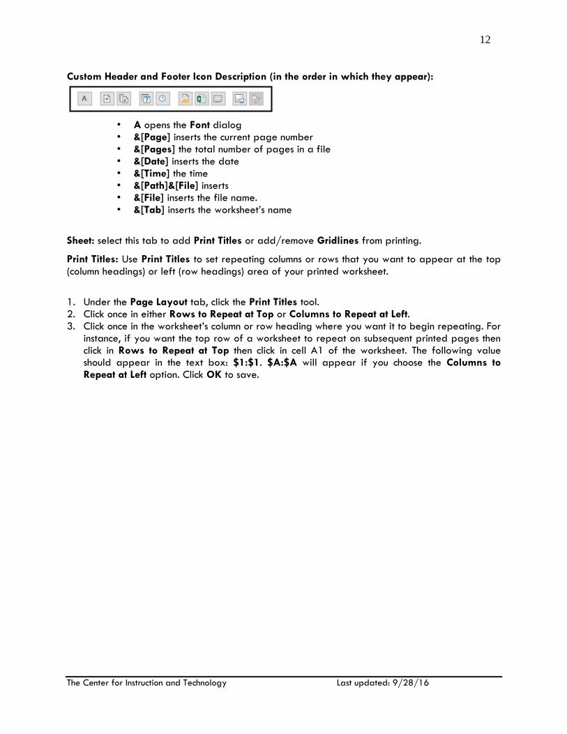
Custom Header and Footer Icon Description (in the order in which they appear):

• A opens the Font dialog • &[Page] inserts the current page number • &[Pages] the total number of pages in a file • &[Date] inserts the date • &[Time] the time • &[Path]&[File] inserts • &[File] inserts the file name. • &[Tab] inserts the worksheet’s name

Sheet: select this tab to add Print Titles or add/remove Gridlines from printing.

Print Titles: Use Print Titles to set repeating columns or rows that you want to appear at the top

(column headings) or left (row headings) area of your printed worksheet.

1. Under the Page Layout tab, click the Print Titles tool. 2. Click once in either Rows to Repeat at Top or Columns to Repeat at Left. 3. Click once in the worksheet’s column or row heading where you want it to begin repeating. For

instance, if you want the top row of a worksheet to repeat on subsequent printed pages then click in Rows to Repeat at Top then click in cell A1 of the worksheet. The following value should appear in the text box: $1:$1. $A:$A will appear if you choose the Columns to Repeat at Left option. Click OK to save.