Exchangeability, Representation Theorems, and Subjectivity

Dale J. Poirier

University of California, Irvine

January 1, 2010

Abstract

According to Bruno de Finetti’s Representation Theorem, exchangeable

beliefs over infinite sequences of observable Bernoulli quantities can be represented

as mixtures of independent coin tossing experiments. Extensions of this theorem

give rise to representations as mixtures of other familiar sampling distributions. This

paper offers a subjectivist primer based on the premise that appreciation of these

theorems enhances understanding of the subjective interpretation of probability, of

its connection to the more prevalent frequentist interpretation, and of its usefulness

as a context in which to view parameters, priors, and likelihoods.

1. Introduction

In his popular notes on the theory of choice, (Kreps, 1988, p. 145) opines that Bruno de

Finetti’s Representation Theorem is the fundamental theorem of statistical inference. de Finetti’s

theorem characterizes likelihood functions in terms of symmetries and invariance. The conceptual

framework begins with an infinite string of observable random quantities taking on values

in a sample space Z. Then it postulates symmetries and invariance for probabilistic assignments to

such strings, and finds a likelihood with the prescribed properties for finite strings of length N. This

2

theorem, and its generalizations: (i) provide tight connections between Bayesian and frequentist

reasoning, (ii) endogenize the choice of likelihood functions, (iii) prove the existence of priors, (iv)

provide an interpretation of parameters which differs from that usually considered, (v) produce

Bayes’ Theorem as a corollary, (vi) produce the Likelihood Principle (LP) and Stopping Rule

Principle (SRP) as corollaries, and (vii) provide a solution to Hume’s problem of induction. This

is a large number of results. Surprisingly, these theorems are rarely discussed in econometrics.

de Finetti developed subjective probability during the 1920s independently of (Ramsey,

1926). de Finetti was an ardent subjectivist. He is famous for the aphorism: “Probability does not

exist.” By this he meant that probability reflects an individual’s beliefs about reality, rather than a

property of reality itself. This viewpoint is also “objective” in the sense of being operationally

measurable, e.g., by means of betting behavior or scoring rules. For example, suppose your true

subjective probability of some event A is p and the scoring rule is quadratic [1(A) - ]2, where 1(A)

is the indicator function and is your announced probability of A occurring. Then minimizing the

expected score implies = p. See (Lindley, 1982) for more details.

This subjectivist interpretation is close to the everyday usage of the term “probability.” Yet

appreciation of the subjectivist interpretation of probability is not wide spread in economics.

Evidence is the widely used Knightian distinction between risk (“known” probabilities/beliefs) and

uncertainty (“unknown” probabilities/beliefs). For the subjectivist, individuals “know” their beliefs,

whether these beliefs are well calibrated (i.e., in empirical agreement) with reality or easily

articulated are different issues. Subjectivist theory takes such knowledge as a primitive assumption,

the same way rational expectations assumes agents know the “true model.” However, unlike

frequentists, subjectivists are not assuming knowledge of a property of reality, rather only

3

1 (Fuchs and Schack, 2004) draw analogies with quantum theory. Is a quantum state an actualproperty of the system it describes? The Bayesian view of quantum states is that it is not. Rather itis solely a function of the observer who contemplates the predictions or actions he might make withregard to quantum measurements.

knowledge of their own perception of reality.1 This distinction is fundamental.

How knowledge of a subjectivist’s beliefs is obtained is not addressed here, although there

is a substantial literature on elicitation: (Garthwaite, Kadane and O’Hagan, 2005) and (O’Hagan et

al., 2006). More important, de Finetti showed that agreement among Bayesian researchers

concerning some aspects of prior beliefs for observables can imply agreement over the likelihood

function. In terms of (Poirier, 1988, 1995), intersubjective agreement among a bevy of Bayesians

leads them to a common parametric window through which to view the observable world, and a

willingness to “agree to disagree” over their priors.

de Finetti’s approach is instrumentalist in nature: past observations are used to make predic-

tions about future observables. Likelihoods, parameters, and random sampling are neither true nor

false. They are merely intermediate fictions, i.e., mathematical constructs. In contrast, realists seek

the “true” data generating process (DGP).

Given the positive integer N, assume an individual’s degrees of belief for N quantities of

interest are derived from the specification of a subjective joint cumulative distribution function

(cdf) P(z1, z2, ..., zN) which is representable in terms of a joint probability density function (pdf) p(z1,

z2, ..., zN) (understood as a mass function in the discrete case), where “zn” denotes a realization of

the corresponding random quantity “Zn .” P(A) and p(A) [and later F(A) and f(A)] are used in a generic

sense, rather than specifying particular functions. For example, Hume’s problem of induction (why

should one expect the future to resemble the past?) requires the predictive pdf of some future

4

2Implicitly, de Finetti assumed the utility of money is linear. He and others suggestedrationalizations like the “stakes are small.” Separation of the concepts of “probability” and “utility”remains a controversial matter (Kadane and Winkler, 1988).

observables conditional on having observed , i.e.,

The essential building block is P(@) for a variety of arguments. The theorems discussed later put

restrictions on P(@). The need for at least some restrictions is obvious since arbitrarily long finite

strings will be discussed. But seemingly weak conditions on arbitrarily long finite strings can

deliver striking results for finite strings, and computation of (1), only involves finite strings of data.

Predictive pdf (1) provides a family of solutions to Hume’s problem. The only restriction

that P(@) must satisfy is coherence, i.e., use of P(@) avoids being made a sure loser regardless of the

outcomes in any betting situation (also known as avoiding Dutch Book).2 This implies that P(@) obeys

the axioms of probability (at least up to finite additivity). Whether (1) leads to good out-of-sample

predictions is a different question for which there is no guaranteed affirmative answer.

Beyond coherence I consider a variety of restrictions to facilitate construction of P(@). Again,

such restrictions should not be thought of as “true” or “false.” They are not meant to be properties

of reality; rather, they are restrictions on one’s beliefs about reality. Other researchers may or may

not find a particular restriction compelling. Part of the art of empirical work is to articulate

restrictions that other researchers are at least willing to entertain if not outright adopt, i.e., to obtain

inter-subjective agreement among a bevy of Bayesians. The simplest such restriction,

exchangeability, is the topic of the next section.

(1)

5

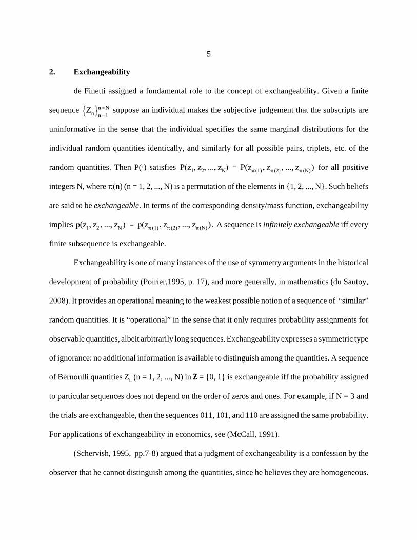
2. Exchangeability

de Finetti assigned a fundamental role to the concept of exchangeability. Given a finite

sequence suppose an individual makes the subjective judgement that the subscripts are

uninformative in the sense that the individual specifies the same marginal distributions for the

individual random quantities identically, and similarly for all possible pairs, triplets, etc. of the

random quantities. Then P(@) satisfies for all positive

integers N, where B(n) (n = 1, 2, ..., N) is a permutation of the elements in {1, 2, ..., N}. Such beliefs

are said to be exchangeable. In terms of the corresponding density/mass function, exchangeability

implies A sequence is infinitely exchangeable iff every

finite subsequence is exchangeable.

Exchangeability is one of many instances of the use of symmetry arguments in the historical

development of probability (Poirier,1995, p. 17), and more generally, in mathematics (du Sautoy,

2008). It provides an operational meaning to the weakest possible notion of a sequence of “similar”

random quantities. It is “operational” in the sense that it only requires probability assignments for

observable quantities, albeit arbitrarily long sequences. Exchangeability expresses a symmetric type

of ignorance: no additional information is available to distinguish among the quantities. A sequence

of Bernoulli quantities Zn (n = 1, 2, ..., N) in Z = {0, 1} is exchangeable iff the probability assigned

to particular sequences does not depend on the order of zeros and ones. For example, if N = 3 and

the trials are exchangeable, then the sequences 011, 101, and 110 are assigned the same probability.

For applications of exchangeability in economics, see (McCall, 1991).

(Schervish, 1995, pp.7-8) argued that a judgment of exchangeability is a confession by the

observer that he cannot distinguish among the quantities, since he believes they are homogeneous.

6

(Gelman et al., 1995, p. 124) remarked: “In practice, ignorance implies exchangeability. Generally,

the less we know about the problem, the more confident we can make claims about

exchangeability.” Arguing against an exchangeability assessment is an admission of the existence

of non-data based information on observables for the problem at hand.

Like iid sequences, the quantities in an exchangeable sequence are identically distributed.

However, unlike in iid sequences, such quantities need not be independent for exchangeable beliefs.

For example, if the quantities are a sample (without replacement) of size N from a finite population

of unknown size N* > N, then they are dependent and exchangeable. Also, the possible dependency

in the case of exchangeable beliefs is what enables the researcher to learn from experience using (1).

Whereas iid sampling is the foundation of frequentist econometrics, exchangeability is the

foundation for Bayesian econometrics. Both serve as the basis for further extensions to incorporate

heterogeneity and dependency across observations. For example, in Section 6 exchangeability will

be weakened to partial exchangeability and a time series model (a first-order Markov process) arises

for the likelihood.

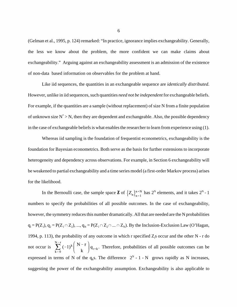
In the Bernoulli case, the sample space Z of has 2N elements, and it takes 2N - 1

numbers to specify the probabilities of all possible outcomes. In the case of exchangeability,

however, the symmetry reduces this number dramatically. All that are needed are the N probabilities

ql = P(Z l), q2 = P(Z l 1 Z2), ..., qN = P(Z l 1 Z2 1 ... 1 ZN). By the Inclusion-Exclusion Law (O’Hagan,

1994, p. 113), the probability of any outcome in which r specified Zis occur and the other N - r do

not occur is Therefore, probabilities of all possible outcomes can be

expressed in terms of N of the qks. The difference 2N - 1 - N grows rapidly as N increases,

suggesting the power of the exchangeability assumption. Exchangeability is also applicable to

7

continuous quantities as the next example shows.

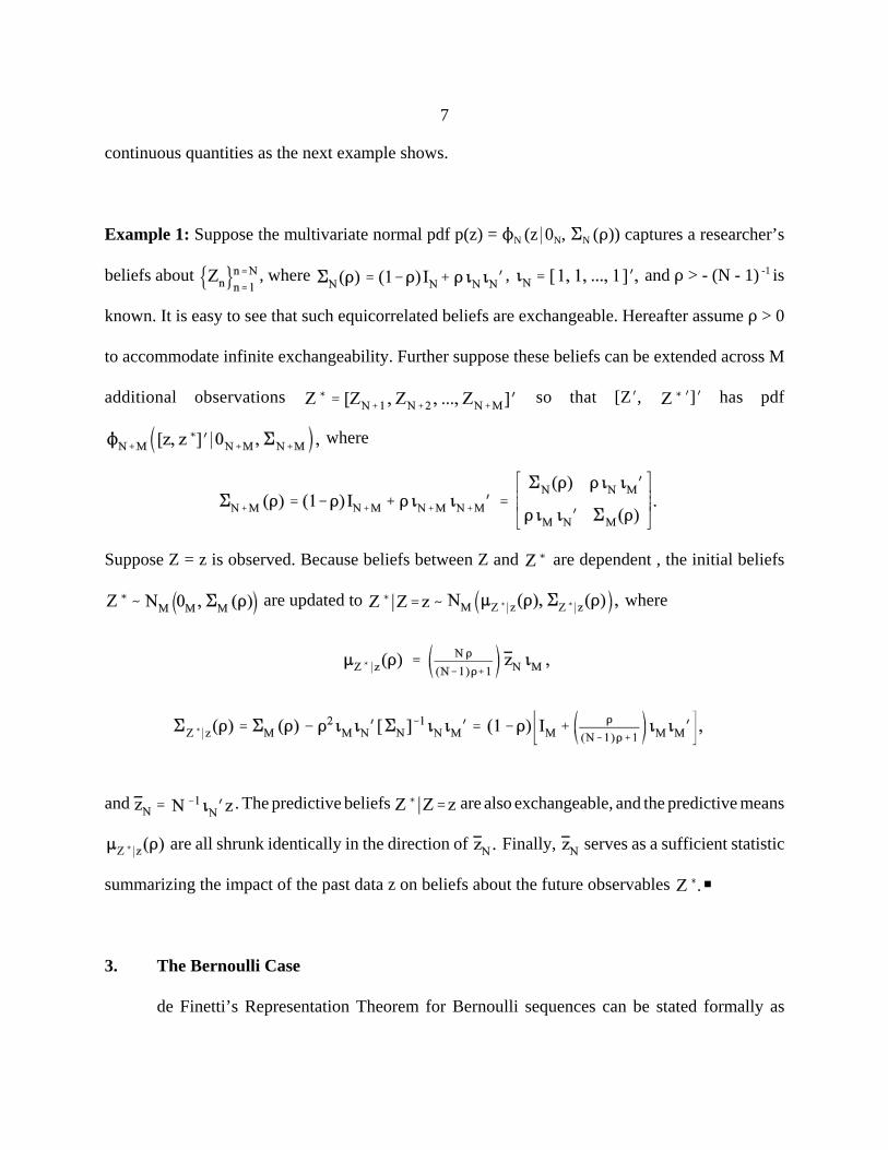
Example 1: Suppose the multivariate normal pdf p(z) = NN (z*0N, EN (D)) captures a researcher’s

beliefs about , where , and D > - (N - 1) -1 is

known. It is easy to see that such equicorrelated beliefs are exchangeable. Hereafter assume D > 0

to accommodate infinite exchangeability. Further suppose these beliefs can be extended across M

additional observations so that [ZN, N]N has pdf

where

Suppose Z = z is observed. Because beliefs between Z and are dependent , the initial beliefs

are updated to where

and . The predictive beliefs are also exchangeable, and the predictive means

are all shrunk identically in the direction of Finally, serves as a sufficient statistic

summarizing the impact of the past data z on beliefs about the future observables P

3. The Bernoulli Case

de Finetti’s Representation Theorem for Bernoulli sequences can be stated formally as

8

(2)

follows (Bernardo and Smith, 1994, pp. 172-173).

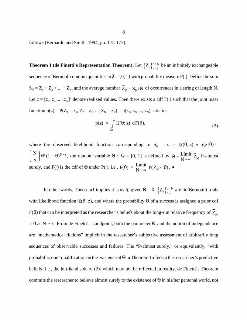
Theorem 1 (de Finetti’s Representation Theorem): Let be an infinitely exchangeable

sequence of Bernoulli random quantities in Z = {0, 1} with probability measure P(@). Define the sum

SN = Z1 + Z2 + ... + ZN, and the average number of occurrences in a string of length N.

Let z = [z1, z2, ..., zN]N denote realized values. Then there exists a cdf F(@) such that the joint mass

function p(z) = P(Z1 = z1, Z2 = z2, ..., ZN = zN) = p(z1, z2, ..., zN) satisfies

where the observed likelihood function corresponding to SN = s is

the random variable 1 0 S / [0, 1] is defined by P-almost

surely, and F(@) is the cdf of 1 under P(@), i.e.,

In other words, Theorem1 implies it is as if, given 1 = 2, are iid Bernoulli trials

with likelihood function ‹(2; z), and where the probability 1 of a success is assigned a prior cdf

F(2) that can be interpreted as the researcher’s beliefs about the long-run relative frequency of

# 2 as N 6 4. From de Finetti’s standpoint, both the parameter 1 and the notion of independence

are “mathematical fictions” implicit in the researcher’s subjective assessment of arbitrarily long

sequences of observable successes and failures. The “P-almost surely,” or equivalently, “with

probability one” qualification on the existence of 1 in Theorem 1refers to the researcher’s predictive

beliefs [i.e., the left-hand side of (2)] which may not be reflected in reality. de Finetti’s Theorem

commits the researcher to believe almost surely to the existence of 1 in his/her personal world, not

9

(3)

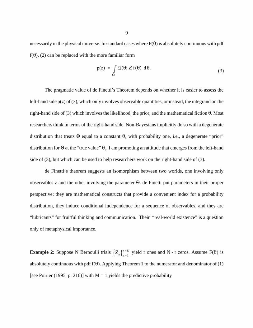
necessarily in the physical universe. In standard cases where F(2) is absolutely continuous with pdf

f(2), (2) can be replaced with the more familiar form

The pragmatic value of de Finetti’s Theorem depends on whether it is easier to assess the

left-hand side p(z) of (3), which only involves observable quantities, or instead, the integrand on the

right-hand side of (3) which involves the likelihood, the prior, and the mathematical fiction 2. Most

researchers think in terms of the right-hand side. Non-Bayesians implicitly do so with a degenerate

distribution that treats 1 equal to a constant 2o with probability one, i.e., a degenerate “prior”

distribution for 1 at the “true value” 2o. I am promoting an attitude that emerges from the left-hand

side of (3), but which can be used to help researchers work on the right-hand side of (3).

de Finetti’s theorem suggests an isomorphism between two worlds, one involving only

observables z and the other involving the parameter 1. de Finetti put parameters in their proper

perspective: they are mathematical constructs that provide a convenient index for a probability

distribution, they induce conditional independence for a sequence of observables, and they are

“lubricants” for fruitful thinking and communication. Their “real-world existence” is a question

only of metaphysical importance.

Example 2: Suppose N Bernoulli trials yield r ones and N - r zeros. Assume F(2) is

absolutely continuous with pdf f(2). Applying Theorem 1 to the numerator and denominator of (1)

[see Poirier (1995, p. 216)] with M = 1 yields the predictive probability

10

3Suppose an urn initially contains r red and b black balls and that, at each stage, a ball isselected at random, then replaced by two of the same color. Let Zn be 1 or 0 accordingly as the nth

ball selected is red or black. Then the Zn (n = 1, 2, 3, ...) are infinitely exchangeable and comprisea Polya urn process. However, not all urn processes are exchangeable. Neither can all exchangeableprocesses can be represented as urn processes. See (Hill, Lane and Sudderth, 1987).

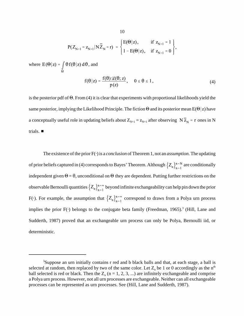
(4)

where , and

is the posterior pdf of 1. From (4) it is clear that experiments with proportional likelihoods yield the

same posterior, implying the Likelihood Principle. The fiction 1 and its posterior mean E(1*z) have

a conceptually useful role in updating beliefs about ZN+1 = zN+1 after observing ones in N

trials. #

The existence of the prior F(@) is a conclusion of Theorem 1, not an assumption. The updating

of prior beliefs captured in (4) corresponds to Bayes’ Theorem. Although are conditionally

independent given 1 = 2, unconditional on 1 they are dependent. Putting further restrictions on the

observable Bernoulli quantities beyond infinite exchangeability can help pin down the prior

F(@). For example, the assumption that correspond to draws from a Polya urn process

implies the prior F(@) belongs to the conjugate beta family (Freedman, 1965).3 (Hill, Lane and

Sudderth, 1987) proved that an exchangeable urn process can only be Polya, Bernoulli iid, or

deterministic.

11

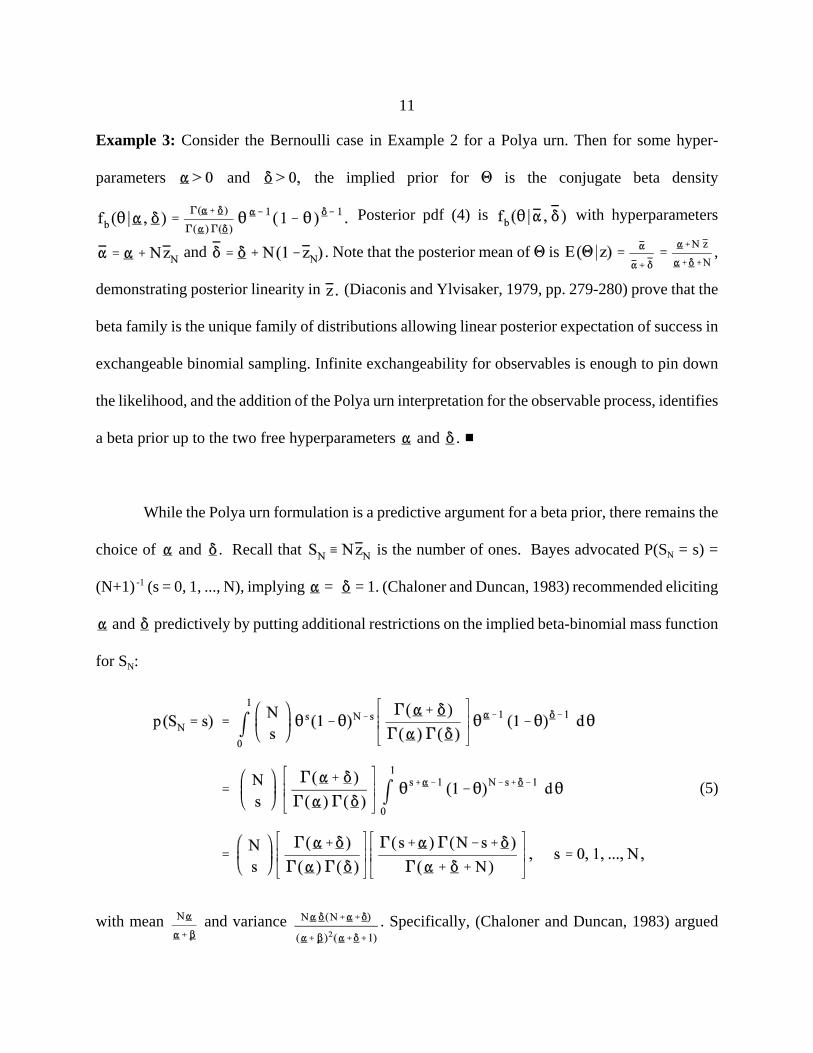
Example 3: Consider the Bernoulli case in Example 2 for a Polya urn. Then for some hyper-

parameters and the implied prior for 1 is the conjugate beta density

Posterior pdf (4) is with hyperparameters

and . Note that the posterior mean of 1 is ,

demonstrating posterior linearity in (Diaconis and Ylvisaker, 1979, pp. 279-280) prove that the

beta family is the unique family of distributions allowing linear posterior expectation of success in

exchangeable binomial sampling. Infinite exchangeability for observables is enough to pin down

the likelihood, and the addition of the Polya urn interpretation for the observable process, identifies

a beta prior up to the two free hyperparameters and . #

While the Polya urn formulation is a predictive argument for a beta prior, there remains the

choice of and . Recall that is the number of ones. Bayes advocated P(SN = s) =

(N+1) -1 (s = 0, 1, ..., N), implying = = 1. (Chaloner and Duncan, 1983) recommended eliciting

and predictively by putting additional restrictions on the implied beta-binomial mass function

for SN:

with mean and variance . Specifically, (Chaloner and Duncan, 1983) argued

(5)

12

(assuming > 1 and > 1) for elicitation in terms of the mode of (5) and the ratios

of probability at m relative to m - 1 and m + 1. In contrast, (Geisser, 1984) discussed

“noninformative” priors for 2 including two members of the beta family other than the uniform: the

limiting improper prior of Haldane ( = = 0) and the proper prior of Jeffreys ( = = ½).

For extension to the multinomial case, see (Bernardo and Smith, 1994, pp. 176-177).

(Johnson, 1924) gave a predictive argument for the multinomial case, similar to Bayes’ argument

in the binomial case.

4. Nonparametric Representation Theorem

de Finetti’s Representation Theorem has been extended to cover exchangeable beliefs

involving random variables more complicated than Bernoulli random variables. The initial

nonparametric case for Euclidean spaces was studied by (de Finetti, 1938). (Hewitt and Savage,

1955) extended the result to arbitrary compact Hausdorff spaces, and (Aldous, 1985) extended it to

random elements with values in a standard Bore1 space. (Dubins and Freedman, 1979) showed that

without any topological assumptions, the result need not hold. The following theorem covers the

general case for real-valued exchangeable random quantities [(Bernardo and Smith, 1994, pp. 178-

179) outlined its proof ].

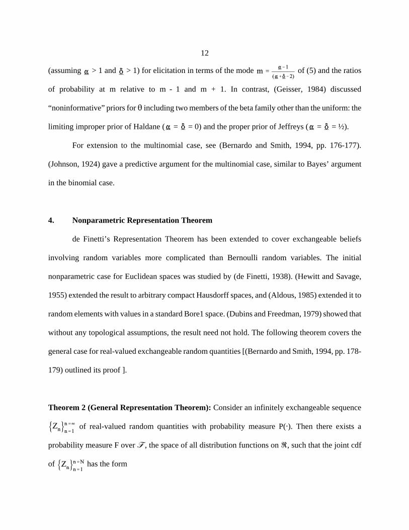
Theorem 2 (General Representation Theorem): Consider an infinitely exchangeable sequence

of real-valued random quantities with probability measure P(@). Then there exists a

probability measure F over ö, the space of all distribution functions on U, such that the joint cdf

of has the form

13

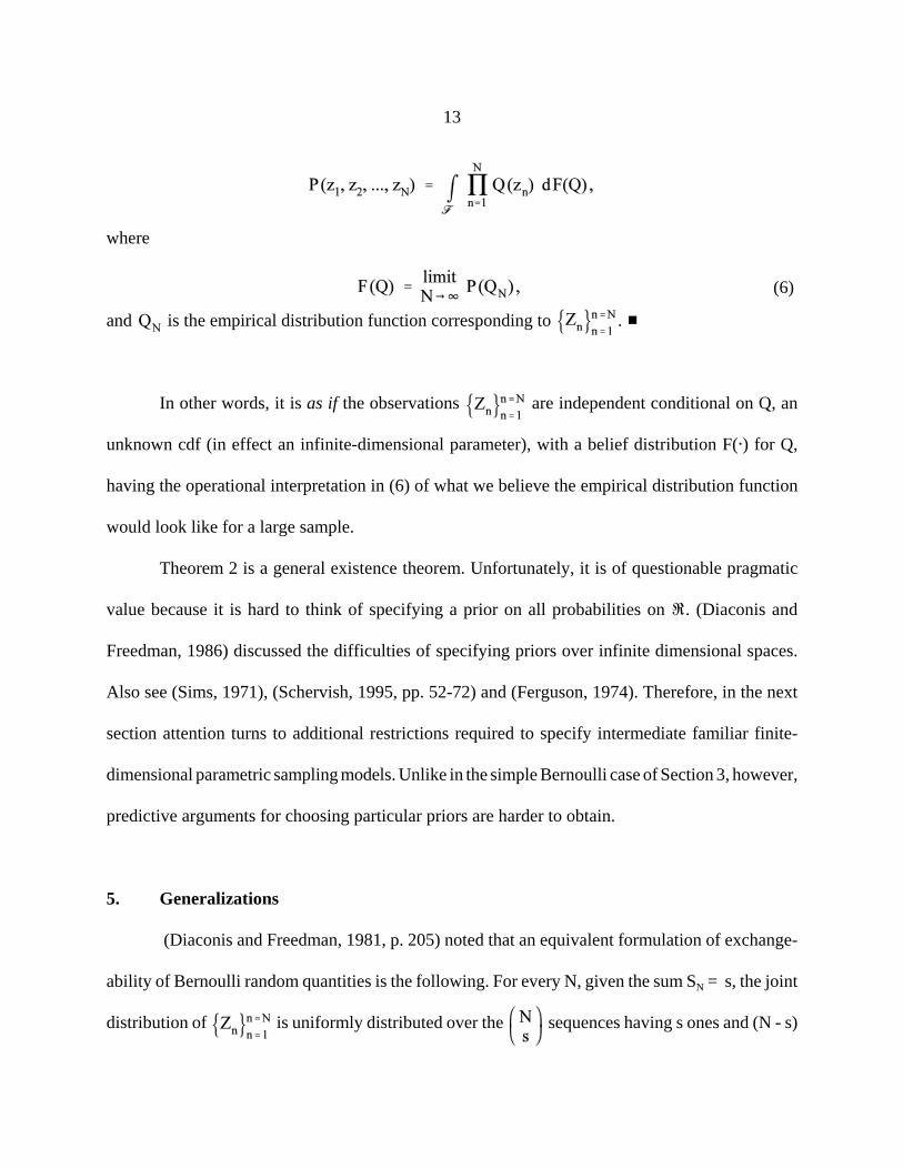
(6)

where

and is the empirical distribution function corresponding to . #

In other words, it is as if the observations are independent conditional on Q, an

unknown cdf (in effect an infinite-dimensional parameter), with a belief distribution F(@) for Q,

having the operational interpretation in (6) of what we believe the empirical distribution function

would look like for a large sample.

Theorem 2 is a general existence theorem. Unfortunately, it is of questionable pragmatic

value because it is hard to think of specifying a prior on all probabilities on U. (Diaconis and

Freedman, 1986) discussed the difficulties of specifying priors over infinite dimensional spaces.

Also see (Sims, 1971), (Schervish, 1995, pp. 52-72) and (Ferguson, 1974). Therefore, in the next

section attention turns to additional restrictions required to specify intermediate familiar finite-

dimensional parametric sampling models. Unlike in the simple Bernoulli case of Section 3, however,

predictive arguments for choosing particular priors are harder to obtain.

5. Generalizations

(Diaconis and Freedman, 1981, p. 205) noted that an equivalent formulation of exchange-

ability of Bernoulli random quantities is the following. For every N, given the sum SN = s, the joint

distribution of is uniformly distributed over the sequences having s ones and (N - s)

14

zeros. In other words, are exchangeable iff the partial sums are sufficient with an

“equiprobable” conditional distribution for Z1, Z2, ..., ZN given SN = s. This section explores

invariance and sufficiency restrictions that deliver familiar sampling distributions in cases more

complicated than Bernoulli variables. In the process these restrictions on observables will yield

parametric families and operationally useful results falling between Theorems 1 and 2.

An example of such a restriction is spherical symmetry. Beliefs regarding z are spherically

symmetric iff p(z) = p(Az) for any N×N orthogonal matrix A (i.e., A-1 = AN) satisfying A4N = 4N (i.e.,

which preserves the unit N-vector 4N). This restriction amounts to rotational invariance of the

coordinate system which fixes distances from the origin. Exchangeability is one form of spherical

symmetry since permutation is one form of orthogonal transformation.

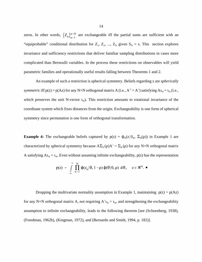
Example 4: The exchangeable beliefs captured by p(z) = NN(z*0N, EN(D)) in Example 1 are

characterized by spherical symmetry because AEN (D)AN = EN (D) for any N×N orthogonal matrix

A satisfying A4N = 4N. Even without assuming infinite exchangeability, p(z) has the representation

Dropping the multivariate normality assumption in Example 1, maintaining p(z) = p(Az)

for any N×N orthogonal matrix A, not requiring AN4N = 4N, and strengthening the exchangeability

assumption to infinite exchangeability, leads to the following theorem [see (Schoenberg, 1938),

(Freedman, 1962b), (Kingman, 1972), and (Bernardo and Smith, 1994, p. 182)].

15

(7)

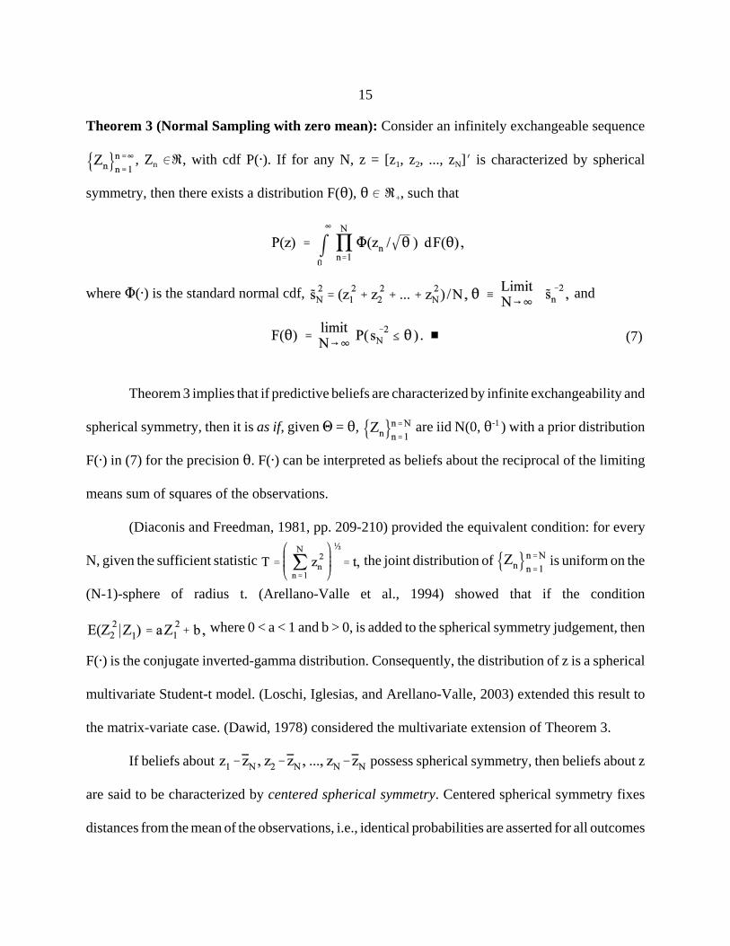
Theorem 3 (Normal Sampling with zero mean): Consider an infinitely exchangeable sequence

, Zn 0U, with cdf P(@). If for any N, z = [z1, z2, ..., zN]N is characterized by spherical

symmetry, then there exists a distribution F(2), 2 0 U+, such that

where M(@) is the standard normal cdf, and

Theorem 3 implies that if predictive beliefs are characterized by infinite exchangeability and

spherical symmetry, then it is as if, given 1 = 2, are iid N(0, 2-1 ) with a prior distribution

F(@) in (7) for the precision 2. F(@) can be interpreted as beliefs about the reciprocal of the limiting

means sum of squares of the observations.

(Diaconis and Freedman, 1981, pp. 209-210) provided the equivalent condition: for every

N, given the sufficient statistic the joint distribution of is uniform on the

(N-1)-sphere of radius t. (Arellano-Valle et al., 1994) showed that if the condition

where 0 < a < 1 and b > 0, is added to the spherical symmetry judgement, then

F(@) is the conjugate inverted-gamma distribution. Consequently, the distribution of z is a spherical

multivariate Student-t model. (Loschi, Iglesias, and Arellano-Valle, 2003) extended this result to

the matrix-variate case. (Dawid, 1978) considered the multivariate extension of Theorem 3.

If beliefs about possess spherical symmetry, then beliefs about z

are said to be characterized by centered spherical symmetry. Centered spherical symmetry fixes

distances from the mean of the observations, i.e., identical probabilities are asserted for all outcomes

16

(8)

(9)

(10)

leading to the same value of When infinite

exchangeability is augmented with centered spherical symmetry, then the familiar normal random

sampling model with unknown mean and unknown precision emerges in the following theorem of

(Smith, 1981). For a proof, see (Bernardo and Smith, 1994, pp. 183-185). Also see (Eaton, Fortini,

and Regazzini,1993, p. 4) for an important qualification.

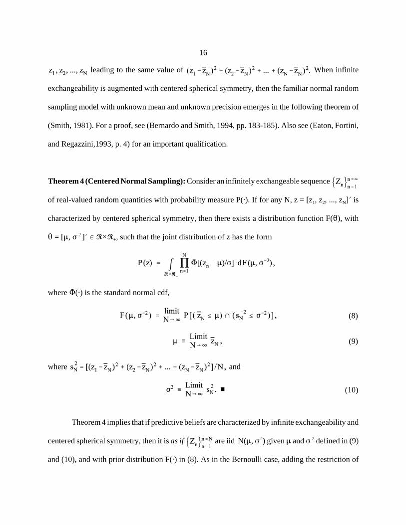
Theorem 4 (Centered Normal Sampling): Consider an infinitely exchangeable sequence

of real-valued random quantities with probability measure P(@). If for any N, z = [z1, z2, ..., zN]N is

characterized by centered spherical symmetry, then there exists a distribution function F(2), with

2 = [:, F-2 ]N 0 U×U+, such that the joint distribution of z has the form

where M(@) is the standard normal cdf,

where and

Theorem 4 implies that if predictive beliefs are characterized by infinite exchangeability and

centered spherical symmetry, then it is as if are iid N(:, F2 ) given : and F-2 defined in (9)

and (10), and with prior distribution F(@) in (8). As in the Bernoulli case, adding the restriction of

17

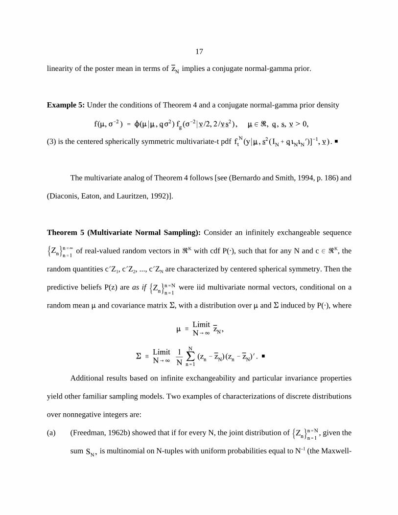
linearity of the poster mean in terms of implies a conjugate normal-gamma prior.

Example 5: Under the conditions of Theorem 4 and a conjugate normal-gamma prior density

(3) is the centered spherically symmetric multivariate-t pdf . P

The multivariate analog of Theorem 4 follows [see (Bernardo and Smith, 1994, p. 186) and

(Diaconis, Eaton, and Lauritzen, 1992)].

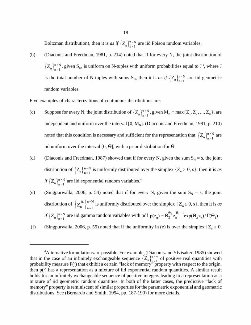
Theorem 5 (Multivariate Normal Sampling): Consider an infinitely exchangeable sequence

of real-valued random vectors in UK with cdf P(@), such that for any N and c 0 UK, the

random quantities cNZ1, cNZ2, ..., cNZN are characterized by centered spherical symmetry. Then the

predictive beliefs P(z) are as if were iid multivariate normal vectors, conditional on a

random mean : and covariance matrix E, with a distribution over : and E induced by P(@), where

Additional results based on infinite exchangeability and particular invariance properties

yield other familiar sampling models. Two examples of characterizations of discrete distributions

over nonnegative integers are:

(a) (Freedman, 1962b) showed that if for every N, the joint distribution of , given the

sum is multinomial on N-tuples with uniform probabilities equal to N–1 (the Maxwell-

18

4Alternative formulations are possible. For example, (Diaconis and Ylvisaker, 1985) showedthat in the case of an infinitely exchangeable sequence of positive real quantities withprobability measure P(@) that exhibit a certain “lack of memory” property with respect to the origin,then p(@) has a representation as a mixture of iid exponential random quantities. A similar resultholds for an infinitely exchangeable sequence of positive integers leading to a representation as amixture of iid geometric random quantities. In both of the latter cases, the predictive “lack ofmemory” property is reminiscent of similar properties for the parametric exponential and geometricdistributions. See (Bernardo and Smith, 1994, pp. 187-190) for more details.

Boltzman distribution), then it is as if are iid Poison random variables.

(b) (Diaconis and Freedman, 1981, p. 214) noted that if for every N, the joint distribution of

, given SN, is uniform on N-tuples with uniform probabilities equal to J-1, where J

is the total number of N-tuples with sums SN, then it is as if are iid geometric

random variables.

Five examples of characterizations of continuous distributions are:

(c) Suppose for every N, the joint distribution of , given MN / max{Z1, Z2 , ..., ZN}, are

independent and uniform over the interval [0, MN]. (Diaconis and Freedman, 1981, p. 210)

noted that this condition is necessary and sufficient for the representation that are

iid uniform over the interval [0, 1], with a prior distribution for 1.

(d) (Diaconis and Freedman, 1987) showed that if for every N, given the sum SN = s, the joint

distribution of is uniformly distributed over the simplex {Zn $ 0, s}, then it is as

if are iid exponential random variables.4

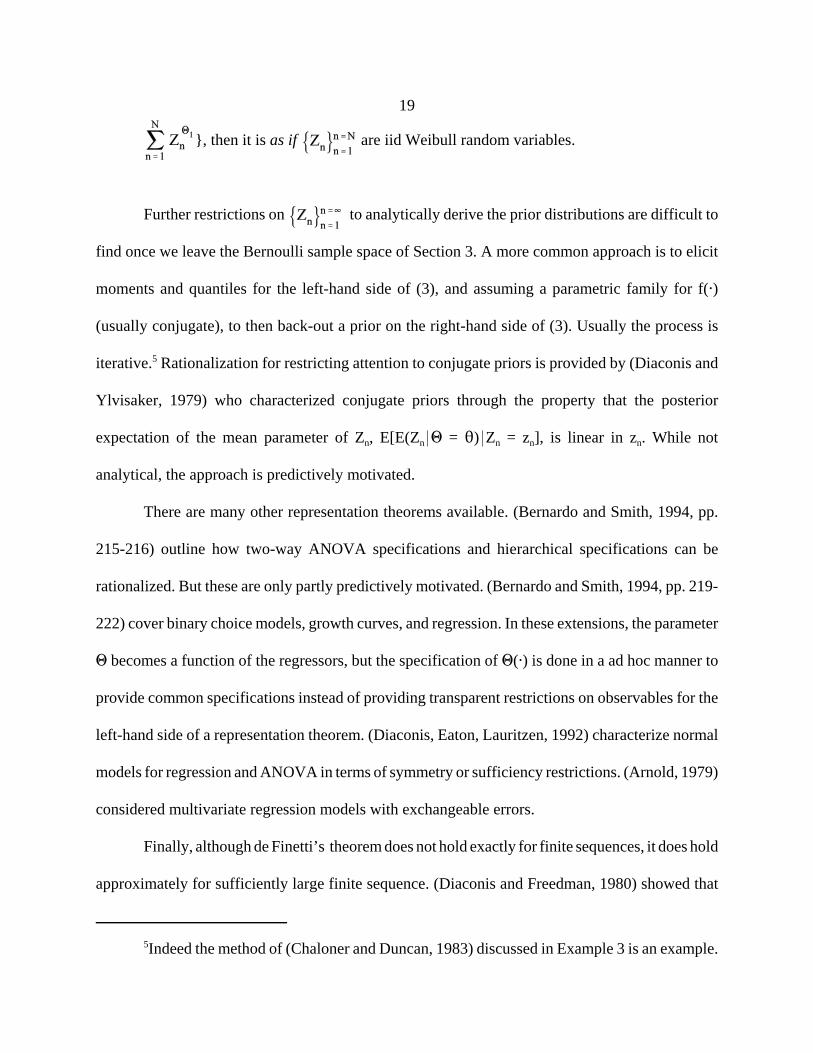
(e) (Singpurwalla, 2006, p. 54) noted that if for every N, given the sum SN = s, the joint

distribution of is uniformly distributed over the simplex { $ 0, s}, then it is as

if are iid gamma random variables with pdf

(f) (Singpurwalla, 2006, p. 55) noted that if the uniformity in (e) is over the simplex {Zn $ 0,

19

5Indeed the method of (Chaloner and Duncan, 1983) discussed in Example 3 is an example.

}, then it is as if are iid Weibull random variables.

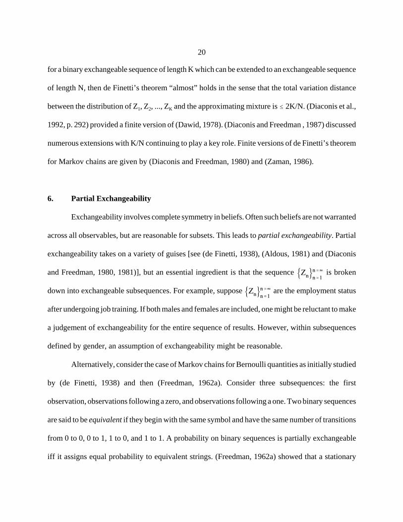
Further restrictions on to analytically derive the prior distributions are difficult to

find once we leave the Bernoulli sample space of Section 3. A more common approach is to elicit

moments and quantiles for the left-hand side of (3), and assuming a parametric family for f(@)

(usually conjugate), to then back-out a prior on the right-hand side of (3). Usually the process is

iterative.5 Rationalization for restricting attention to conjugate priors is provided by (Diaconis and

Ylvisaker, 1979) who characterized conjugate priors through the property that the posterior

expectation of the mean parameter of Zn, E[E(Zn*1 = 2)*Zn = zn], is linear in zn. While not

analytical, the approach is predictively motivated.

There are many other representation theorems available. (Bernardo and Smith, 1994, pp.

215-216) outline how two-way ANOVA specifications and hierarchical specifications can be

rationalized. But these are only partly predictively motivated. (Bernardo and Smith, 1994, pp. 219-

222) cover binary choice models, growth curves, and regression. In these extensions, the parameter

1 becomes a function of the regressors, but the specification of 1(@) is done in a ad hoc manner to

provide common specifications instead of providing transparent restrictions on observables for the

left-hand side of a representation theorem. (Diaconis, Eaton, Lauritzen, 1992) characterize normal

models for regression and ANOVA in terms of symmetry or sufficiency restrictions. (Arnold, 1979)

considered multivariate regression models with exchangeable errors.

Finally, although de Finetti’s theorem does not hold exactly for finite sequences, it does hold

approximately for sufficiently large finite sequence. (Diaconis and Freedman, 1980) showed that

20

for a binary exchangeable sequence of length K which can be extended to an exchangeable sequence

of length N, then de Finetti’s theorem “almost” holds in the sense that the total variation distance

between the distribution of Z1, Z2, ..., ZK and the approximating mixture is # 2K/N. (Diaconis et al.,

1992, p. 292) provided a finite version of (Dawid, 1978). (Diaconis and Freedman , 1987) discussed

numerous extensions with K/N continuing to play a key role. Finite versions of de Finetti’s theorem

for Markov chains are given by (Diaconis and Freedman, 1980) and (Zaman, 1986).

6. Partial Exchangeability

Exchangeability involves complete symmetry in beliefs. Often such beliefs are not warranted

across all observables, but are reasonable for subsets. This leads to partial exchangeability. Partial

exchangeability takes on a variety of guises [see (de Finetti, 1938), (Aldous, 1981) and (Diaconis

and Freedman, 1980, 1981)], but an essential ingredient is that the sequence is broken

down into exchangeable subsequences. For example, suppose are the employment status

after undergoing job training. If both males and females are included, one might be reluctant to make

a judgement of exchangeability for the entire sequence of results. However, within subsequences

defined by gender, an assumption of exchangeability might be reasonable.

Alternatively, consider the case of Markov chains for Bernoulli quantities as initially studied

by (de Finetti, 1938) and then (Freedman, 1962a). Consider three subsequences: the first

observation, observations following a zero, and observations following a one. Two binary sequences

are said to be equivalent if they begin with the same symbol and have the same number of transitions

from 0 to 0, 0 to 1, 1 to 0, and 1 to 1. A probability on binary sequences is partially exchangeable

iff it assigns equal probability to equivalent strings. (Freedman, 1962a) showed that a stationary

21

partially exchangeable process is a mixture of Markov chains. (Diaconis and Freedman, 1980a)

eliminated the stationary assumption. To get a mixture of Markov chains in this case, infinitely

many returns to the starting state are needed. Extensions to countable situations are straightforward,

but extensions to more general spaces are more complex [see (Diaconis, 1988)].

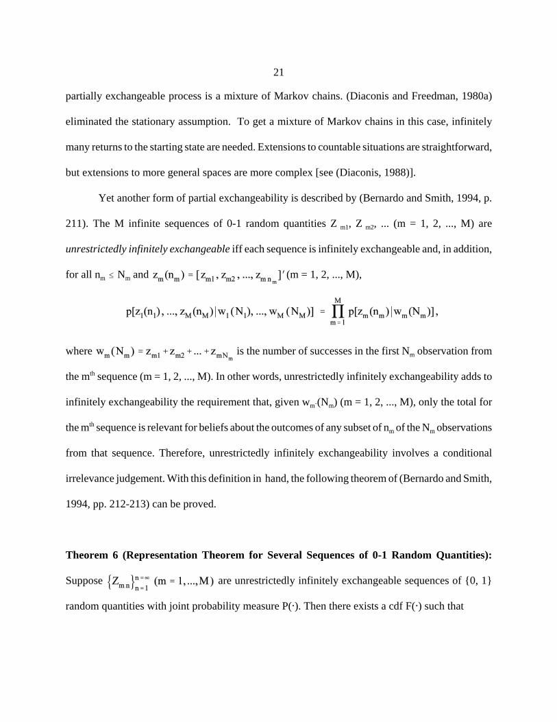
Yet another form of partial exchangeability is described by (Bernardo and Smith, 1994, p.

211). The M infinite sequences of 0-1 random quantities Z m1, Z m2, ... (m = 1, 2, ..., M) are

unrestrictedly infinitely exchangeable iff each sequence is infinitely exchangeable and, in addition,

for all nm # Nm and (m = 1, 2, ..., M),

where is the number of successes in the first Nm observation from

the mth sequence (m = 1, 2, ..., M). In other words, unrestrictedly infinitely exchangeability adds to

infinitely exchangeability the requirement that, given wm`(Nm) (m = 1, 2, ..., M), only the total for

the mth sequence is relevant for beliefs about the outcomes of any subset of nm of the Nm observations

from that sequence. Therefore, unrestrictedly infinitely exchangeability involves a conditional

irrelevance judgement. With this definition in hand, the following theorem of (Bernardo and Smith,

1994, pp. 212-213) can be proved.

Theorem 6 (Representation Theorem for Several Sequences of 0-1 Random Quantities):

Suppose are unrestrictedly infinitely exchangeable sequences of {0, 1}

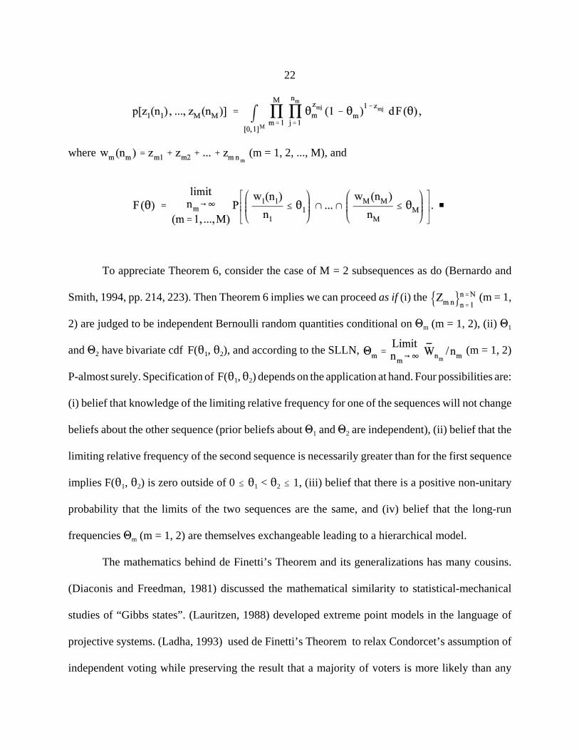
random quantities with joint probability measure P(@). Then there exists a cdf F(@) such that

22

where (m = 1, 2, ..., M), and

To appreciate Theorem 6, consider the case of M = 2 subsequences as do (Bernardo and

Smith, 1994, pp. 214, 223). Then Theorem 6 implies we can proceed as if (i) the (m = 1,

2) are judged to be independent Bernoulli random quantities conditional on 1m (m = 1, 2), (ii) 11

and 12 have bivariate cdf F(21, 22), and according to the SLLN, (m = 1, 2)

P-almost surely. Specification of F(21, 22) depends on the application at hand. Four possibilities are:

(i) belief that knowledge of the limiting relative frequency for one of the sequences will not change

beliefs about the other sequence (prior beliefs about 11 and 12 are independent), (ii) belief that the

limiting relative frequency of the second sequence is necessarily greater than for the first sequence

implies F(21, 22) is zero outside of 0 # 21 < 22 # 1, (iii) belief that there is a positive non-unitary

probability that the limits of the two sequences are the same, and (iv) belief that the long-run

frequencies 1m (m = 1, 2) are themselves exchangeable leading to a hierarchical model.

The mathematics behind de Finetti’s Theorem and its generalizations has many cousins.

(Diaconis and Freedman, 1981) discussed the mathematical similarity to statistical-mechanical

studies of “Gibbs states”. (Lauritzen, 1988) developed extreme point models in the language of

projective systems. (Ladha, 1993) used de Finetti’s Theorem to relax Condorcet’s assumption of

independent voting while preserving the result that a majority of voters is more likely than any

23

single voter to choose the better of two alternatives. The mathematics of representation theorems

is both deep and broad.

7. Conclusions

“... one could say that for him (de Finetti) Bayesianism represents the

crossroads where pragmatism and empiricism meet subjectivism. He thinks one

needs to be Bayesian in order to be subjectivist, but on the other hand subjectivism

is a choice to be made if one embraces a pragmatist and empiricist philosophy.”

(Galavotti, 2001, p. 165)

I believe the case has been made for Bayesianism in the sense of de Finetti. I have promoted

a subjective attitude emerging from the left-hand side of (3), but which can be used to help

researchers work on the more customary right-hand side. This change of emphasis from parameters

to observables puts the former in a subsidiary role. Less fascination with parameters can be healthy.

The prior f(@), which is implied (not assumed) by a representation theorem, is always proper. This

rules out the usual priors used in objective Bayesian analysis [see (Berger, 2004)]. But interestingly,

exchangeability, which is an admission of no additional information regarding otherwise similar

observable quantities, implies the use of a proper prior for the mathematical fiction 1. To pin down

this prior further requires additional assumptions about observable sequences (e.g., the Polya urn

assumption in Example 3).

If the researcher finds it more convenient to think in terms of the right-hand side of (3) (say,

because the researcher has a theoretical framework in which to interpret 1), then by all means elicit

24

a personal prior for 1 or consider the sensitivity of the posterior with respect to professional

viewpoints of interest defined parametrically. But given that most people find prior choice difficult,

a representation theorem provides an alternative way to use subjective information about

observables to facilitate prior choice for 1.

Even when a representation theorem is not available for a given parametric likelihood (say,

because it is unclear what restrictions on the left-had side of (3) would be sufficient to imply this

choice of likelihood), the spirit of this discussion has hopefully not been lost on the reader.

Representation theorems reflect a healthy attitude toward parametric likelihoods: they are not

intended to be “true” properties of reality, but rather useful windows for viewing the observable

world, communicating with other researchers, and making inferences regarding future observables.

References

Aldous, D. (1981). ‘Representations for Partially Exchangeable Arrays of Random Variables’.

Journal of Multivariate Analysis, 11: 581-598.

Aldous, D. (1985). ‘Exchangeability and Related Topics’, in: P. L. Hennequin (ed.), Ècole d’Èté de

Probabilités de Saint-Flour XIII - 1983. Berlin: Springer, 1-198.

Arellano-Valle, R. B., H. Bolfarine and P. Iglesias (1994). ‘A Predictivistic Interpretation of the

Multivariate t Distribution’. Test, 3: 221–236.

25

Arnold, S. F. (1979). ‘Linear Models with Exchangeably Distributed Errors’. Journal of the

American Statistical Association, 74: 194-199.

Berger. J. O. (2004). ‘The Case for Objective Bayesian Analysis’. Bayesian Analysis, 1: 1-17.

Bernardo, J. M. and A. F. M. Smith (1994). Bayesian Theory. New York: Wiley.

Chaloner, K. M. and G. T. Duncan. (1983). ‘Assessment of a Beta Prior Distribution: PM

Elicitation’. Statistician, 32: 174-180.

Dawid, A. P. (1978). ‘Extendibility of Spherical Matrix Distributions,’ Journal of Multivariate

Analysis, 8: 559-566.

de Finetti, B. (1938). ‘Sur la Condition d’équivalence Partielle’. Actualités Scientfiques et

Industrielles 739. Paris: Herman and Cii.

Diaconis, P. (1988). ‘Recent Progress on de Finetti’s Notions of Exchangeability’, in: J. M.

Bernardo, M. H. DeGroot, D. V. Lindley, and A. F. M. Smith (eds.), Bayesian Statistics 3. Oxford:

Oxford University Press, 111-125.

Diaconis, P. and D. Freedman (1980). ‘de Finetti’s Theorem for Markov Chains’. Annals of

Probability, 8: 115-130.

26

Diaconis, P. and D. Freedman (1981). ‘Partial Exchangeability and Sufficiency’, in J. K. Ghosh and

J. Roy (eds.), Proc. Indian Statistical Institute Golden Jubelee International Conference on Statistics:

Applications and New Directions. Calcutta: Indian Statistical Institute, 205-236.

Diaconis, P. and D. Freedman (1986). ‘On the Consistency of Bayes Estimates (with discussion)’.

Annals of Statistics, 14: 1-67.

Diaconis, P. and D. Freedman. (1987). ‘A Dozen de Finetti-style Results in Search of a Theory’.

Annals of the Institute Henri Poincare, 23: 394-423.

Diaconis, P. and D. Ylvisaker (1979). ‘Conjugate Priors for Exponential Families’. Annals of

Statistics, 7: 269-281.

Diaconis, P. and D. Ylvisaker (1985). ‘Quantifying Prior Opinion’ (with discussion), in: J. M.

Bernardo, M. H. DeGroot, D. V. Lindley and A. F. M. Smith (eds.), Bayesian Statistics 2.

Amsterdam: North-Holland, 133-156.

Diaconis, P. W., M. L. Eaton, S. L. Lauritzen (1992). ‘Finite De Finetti Theorems in Linear Models

and Multivariate Analysis’. Scandinavian Journal of Statistics, 19: 289-315

du Sautoy, M. (2008). Finding Moonshine: A Mathematician’s Journey Through Symmetry.

London: Fourth Estate.

27

Dubins, L. E. and D. A. Freedman (1979). ‘Exchangeable Processes Need Not to be Mixtures of

Independent Identically Distributed Random Variables’. Zeitschrift für Wahrscheinlichkeitstheorie

und verwandte Gebiete, 48: 115-132.

Eaton, M. L., S. Fortini, and E. Regazzini (1993). ‘Spherical Symmetry: An Elementary

Justification’. Journal of the Italian Statistical Association, 1: 1-16.

Ferguson, T. S. (1974). ‘Prior Distributions on Spaces of Probability Measures’. Annals of

Statistics, 2: 615-629.

Freedman, D. (1962a). ‘Mixtures of Markov Processes’. Annals of Mathematical Statistics, 33:

114-118.

Freedman, D. (1962b). ‘Invariants Under Mixing which Generalize de Finetti’s Theorem’. Annals

of Mathematical Statistics, 33: 916-923.

Freedman, D. (1965). ‘Bernard Friedman’s Urn’. Annals of Mathematical Statistics, 36: 956-970.

Fuchs, C. A. and R. Schack (2004). ‘Unknown Quantum States and Operations, a Bayesian View’,

in: M. G. A. Paris and J. Ìehá…ek (eds.), Quantum Estimation Theory. Berlin: Springer.

Galavotti, M. C. (2001). ‘Subjectivism, Objectivism and Objectivity in Bruno de Finetti’s

28

Bayesianism’. in: D. Cornfield and J. Williamson (eds.), Foundations of Bayesianism. Kluwer, 161-

174.

Garthwaite, P. H., J. B. Kadane, and A. O’Hagan (2005). ‘Statistical Methods for Eliciting

Probability Distributions’. Journal of the American Statistical Association, 100: 680-700.

Geisser, S. (1984). ‘On Prior Distributions for Binary Trials (with discussion)’. American

Statistician, 38: 244-251.

Gelman, A., J. B. Carlin, H. S. Stern and D. B. Rubin (1995). Bayesian Data Analysis. London:

Chapman & Hall.

Hewitt, E. and Savage, L. J. (1955). ‘Symmetric Measures on Cartesian Products’. Transactions of

the American Mathematical Society, 80: 470-501.

Hill, B., D. Lane, and W. Suddreth (1987). ‘Exchangeable Urn Processes’. Annals of Probability,

15: 1586-1592.

Johnson, W. E. (1924). Logic, Part III. The Logical Foundations of Science, Cambridge: Cambridge

University Press.

Kadane, J. B., and Winkler, R. L. (1988). ‘Separating Probability Elicitation From Utilities’. Journal

29

of the American Statistical Association, 83: 357–363.

Kingman, J. F. C. (1972). ‘On Random Sequences with Spherical Symmetry’. Biometrika, 59:

492-494.

Kreps, D. M. (1988). Notes on the Theory of Choice. Boulder: Westview Press.

Ladha, K. K. (1993). ‘Condorcet’s Jury Theorem in Light of de Finetti’s Theorem: Majority-rule

Voting with Correlated Votes’. Social Choice and Welfare, 10: 69-85.

Lauritzen, S. L. (1988). Extremal Families and Systems of Sufficient Statistics, Lecture Notes in

Statistics 49. Springer, New York.

Lindley, D. V. (1982). ‘Scoring Rules and the Inevitability of Probability’. International Statistical

Review, 50: 1-26.

Loschi, R. H., P. L. Iglesias, and R. B. Arellano-Valle (2003). ‘Predictivistic Characterizations of

Multivariate Student-t Models’. Journal of Multivariate Analysis, 85: 10–23.

McCall, J. J. (1991). ‘Exchangeability and Its Economic Applications’. Journal of Economic

Dynamics and Control, 15: 549-568.

30

O’Hagan, A. (1994). Kendall’s Advanced Theory of Statistics, Vol. 2B, Bayesian Inference.

London: Halsted Press.

O’Hagan, A., C. E. Buck, A. Daneshkhah, J. R. Eiser, P. H. Garthwaite, D. J. Jenkinson, J. E.

Oakley, and T. Rakow (2006). Uncertain Judgements: Eliciting Experts’ Probabilities. NY: Wiley.

Poirier, D. J. (1988). ‘Frequentist and Subjectivist Perspectives on the Problems of Model

Building in Economics (with discussion)’. Journal of Economic Perspectives, 2: 121-170.

Poirier, D. J. (1995). Intermediate Statistics and Econometrics: A Comparative Approach.

Cambridge: MIT Press.

Ramsey, F. P. (1926). ‘Truth and Probability’, in Ramsey, 1931, The Foundations of Mathematics

and other Logical Essays, Ch. VII, ed. R. B. Braithwaite, London: Kegan, Paul, Trench, Trubner &

Co. (New York: Harcourt, Brace and Company), 156-198.

Schervish, M. J. (1995). Theory of Statistics. NY: Springer-Verlag.

Schoenberg, I. J. (1938). ‘Metric Spaces and Positive Definite Functions’. Transactions of the

American Mathematical Society, 44: 522-536.

Sims, C. A. (1971). Distributed Lag Estimation When the Parameter Space in Explicitly Infinite-

31

Dimensional. Annals of Mathematical Statistics 42: 1622-1636.

Singpurwalla, N. (2006). Reliability and Risk: A Bayesian Perspective. Chicester: Wiley.

Smith, A. F. M. (1981). ‘On Random Sequences with Centred Spherical Symmetry’. Journal of the

Royal Statistical Society, 43, Series B: 208-209.

Zaman, A. (1986). ‘A Finite Form of de Finetti’s Theorem for Stationary Markov Exchangeability’.

Annals of Probability, 14: 1418-1427.