exotic chaotic patterns - ppke
TRANSCRIPT

spatio-temporal patterns and
active wave computing
Ph.D. Dissertation
istván petrás
Analogical and Neural Computing Systems Laboratory
Computer and Automation Institute Hungarian Academy of Sciences
2004


“... How dear are your thoughts to me, O God! How great is the number of them! If I made up their num-ber, it would be more than the grains of sand ...”
(Psalm of David)


Acknowledgement
I would like to say thank you
To my professor, prof. Tamás Roska, who helped and supported me in many ways.
To my Parents.
To prof. Marco Gilli, who provided me with fruitful discussion, ideas and help.
To prof. Leon O. Chua, who accepted me in his Nonlinear Research Laboratory in University of California at Berkeley
To prof. Joos Vandewalle, ar Electrical Engineering Department of Katholieke Universiteit Leuven where I spent a month.
To my colleagues, with whom I discussed ideas and question and worked together in dif-ferent projects:
Dávid Bálya, György Cserey, Péter Földesy, Viktor Gál, Péter Jónás, Kristóf Karacs, László Kék, László Orzó, Csaba Rekeczky, István Szatmári, Zoltán Szlávik, Gergely Tímár; Seniors: Ákos Zarándy, Péter Szolgay, Tamás Szirányi. To Katalin Keserű (assistant) and Gabriella Kék (secretary) for their kind help.
To the MTA-SZTAKI where I work and spent my Ph.D. student years (http://lab.analogic.sztaki.hu/)
To my professors and teachers in Veszprémi Egyetem (University of Veszprém, http://www.vein.hu/) Bánki Donáth Műszaki Főiskola (Bánki Donáth Politechnic, http://www.banki.hu/) Erkel Ferenc Gimnázium (Secondary school, http://www.erkel.hu/)

Gyulai 1. számú Általános Iskola (Elementary school) To my town, Gyula (http://www.gyula.hu/) where I was born and grew up.
I would like to acknowledge the financial support of the Hungarian National Research and Development Program: TeleSense NKFP 2001/02/035 European Community, “Information Society Technologies” Program: Locust IST-2001-38097


Table Of Contents
ACKNOWLEDGEMENT............................................................................................................................................ 5 1. INTRODUCTION................................................................................................................................................ 1 2. CNN PARADIGM................................................................................................................................................. 9
2.1 CNN PARADIGM .......................................................................................................................................10 2.1.1 Basic notations...........................................................................................................................................10 2.1.2 Mathematical formulation.....................................................................................................................11 2.1.3 Space invariant linear CNN................................................................................................................13 2.1.4 Autonomous CNN and PDEs...............................................................................................................14
2.2 CNN UNIVERSAL MACHINE – ANALOGIC COMPUTER...................................................15 2.2.1 Architecture.................................................................................................................................................15 2.2.2 Algorithm design .......................................................................................................................................16 2.2.3 Hardware implementations...................................................................................................................17 2.2.4 Application development environment...............................................................................................18
3. DYNAMIC PATTERNS.................................................................................................................................21 3.1 CNN MODEL...............................................................................................................................................23
3.1.1 Simulation ...................................................................................................................................................23 3.1.2 Programmable chip measurements – the experimental test bed ................................................23
3.2 THE EFFECT OF VERTICAL COUPLING........................................................................................23 3.2.1 Positive vertical coupling (r > 0).......................................................................................................25 3.2.2 Negative vertical coupling (r < 0) .....................................................................................................26
3.3 THE EFFECT OF THE CENTRAL TEMPLATE ELEMENT .....................................................27 3.3.1 Simulation ...................................................................................................................................................28 3.3.2 Programmed chip measurement ...........................................................................................................32 3.3.3 Spatio-temporal signatures ...................................................................................................................35
3.4 THE EFFECT OF THE CONSTANT INPUT AND INITIAL STATE.....................................37 3.4.1 Periodic-chaotic transition....................................................................................................................37 3.4.2 Stable-periodic transition ......................................................................................................................38
3.5 1D CHAOS .......................................................................................................................................................39 3.6 ADDITIONAL TRAVELING PATTERN EXAMPLES ...................................................................40
3.6.1 Wave shadow .............................................................................................................................................40 3.6.2 “Four pixels” examples ............................................................................................................................42
3.7 SIMULATION TIME VS. REAL-TIME MEASUREMENTS.........................................................43 4. COMPLEX DYNAMICS IN 1D CNN..................................................................................................45
4.1 EFFECT OF BOUNDARY CONDITION..............................................................................................46 4.2 NONLINEAR DYNAMICS ........................................................................................................................52
4.2.1 Study of 1D CNN with a selected template..................................................................................... 52 4.2.2 Coexistence of attractors in a 4×1 CNN.......................................................................................... 60 4.2.3 Effect of the perturbation of template parameters on the exponents ........................................ 62 4.2.4 Higher dimension - Hyperchaos.......................................................................................................... 63
5. SPECIAL WAVE OPERATOR ..................................................................................................................69 5.1 SHAPE DEFORMATION............................................................................................................................71 5.2 NUMBER OF LINEAR CELLS .................................................................................................................73
5.2.1 Horizontally or vertically aligned boundary region .................................................................... 73 5.2.2 Boundary region aligned with π/4.................................................................................................... 75
5.3 THE CNN AS A CURVE EVOLUTION COMPUTER .................................................................78 5.3.1 Examples ...................................................................................................................................................... 85 5.3.2 Connection to bipolar waves ................................................................................................................. 88
6. APPLICATION AND EXPERIMENTS .............................................................................................91 6.1 WAVE COMPUTING..................................................................................................................................91
6.1.1 Direction constrained wave.................................................................................................................. 91 6.1.2 Bipolar waves ........................................................................................................................................... 93 6.1.3 Curvature and concavity based object decomposition .................................................................. 94 6.1.4 Fork detection ............................................................................................................................................. 95 6.1.5 Hand orientation detection.................................................................................................................... 96 6.1.6 Texton segmentation ............................................................................................................................... 98
6.2 MOBILE NAVIGATION UNIT ...............................................................................................................98 6.2.1 Hardware infrastructure....................................................................................................................... 98 6.2.2 Software infrastructure........................................................................................................................101 6.2.3 Optic flow estimation.............................................................................................................................102 6.2.4 Visual collision avoidance...................................................................................................................104 6.2.5 Feature detection .....................................................................................................................................106
6.3 COMPLEX SPATIO–TEMPORAL WAVE EXPERIMENTS WITH CNN......................... 106 6.3.1 Mathematical model ..............................................................................................................................106 6.3.2 Stored programmability ........................................................................................................................107 6.3.3 Wave phenomenon..................................................................................................................................108
REFERENCES................................................................................................................................................................. 115 APPENDIX A.................................................................................................................................................................... 127 APPENDIX B.................................................................................................................................................................... 129


1. INTRODUCTION
1. Introduction
atterns and waves are so “natural” that we do not pay particular attention to them in our life normally. We do not even notice most of them. Yet, they are inherent phe-
nomena of our world. In general sense pattern can be an arrangement of matter, energy or other substance. Patterns are around and in us everywhere and they play an important role even in our understanding and perceiving. A wave is created when the state or position of a substance locally changes spatially and temporally synchronized in such a way that this local change propagates. In a broad sense the pattern is a distribution of a property of the medium. A kind of mixture of waves and patterns is also possible: a traveling pattern can form a wave, or from the other point of view a wave can have texture (see Fig. 1 and Fig. 2). In this case special local interactions form and maintain an arrangement or texture in the spreading wave. An interesting example is shown in the third thesis of this dissertation.
P
Figure 1. Novel type of traveling nonlinear wave. It propagates to a finite distance. After that distance is reached only ripples along the edge travel. Consecutive snapshots of the active medium.
Figure 2. Novel type of traveling pattern. Consecutive snapshots of the active medium.
1

1. INTRODUCTION
Figure 3. Special trigger wave. Observe the smoothing of the sharp edges along the contour.
When we are talking about waves one usually thinks of the classical waves that spread in conservative systems. An example of this well-known by everybody is the surface waves of water. In this case, the energy pumped into the system is conserved.
Nonlinear wave can also be formed in water. Russel [2] discovered the so–called “soli-tary waves” or soliton. This is a wave consisting of a single elevation, of height not neces-sarily small compared to the depth of the fluid. If properly started it can travel mostly without change in a uniform canal. Similarly, in the ocean an isolated giant wave triggered by earthquake travels thousands of kilometres without losing its shape and energy. At pre-sent solitons are typical objects in hydrodynamics, acoustics, optics, plasma physics, theory of superconductivity, etc.
Figure 4. Snapshots of different autowaves. Trigger, target and spiral waves. These results were measured on a programmable analog VLSI array computer.
Nonlinear waves spreading in excitable (non-conservative) medium differs from the “classical” waves. Waves in the classical sense (e.g. electromagnetic waves spreading in vacuum) mostly constitute physically closed system in themselves, i.e. they do not interact with other systems e.g. with a media. It is enough to integrate the state variables of the closed system into the energy balance of such waves and the energy computed taking them into account remains constant during the process. In the case of the excitable waves the conservation of energy is hold only when one considers the state of the wave and the media and the interaction between them. However it seems not to be hold if we consider the wave as a subsystem.
Nonlinear waves spread at the expense of energy stored in the media such a way that an activated point activates the neighboring points of the medium. From this comes the name autowaves [3] coined by R.V. Khorlov, as an abbreviation for autonomous waves. The name expresses well the property that the propagation is self–sustaining. The dispersion and de-cay properties of a spreading autowave are characteristically different from that of the clas-sical ones: the wave does not decay nor the waveform is distorted during the propagation.
2

1. INTRODUCTION
Autowaves cannot be reflected from the boundaries, nor can they interfere. When collid-ing, autowaves annihilate each other. Diffraction is the only property classical and autowaves have in common. Table 1. shows the comparison of classical and autowaves.
Property Classical waves Autowaves 1. conservation of energy + – 2. conservation of am-
plitude and wave form – +
3. reversibility – + 4. reflection + – 5. interference + – 6. diffraction + + 7. annihilation – +
Table 1. Comparison of classical and autowave properties [1].
Up to now, several types of active waves were described and studied. Depending on the nature of the observed phenomena different names have been used in literature, such as autowaves, traveling waves or trigger/triggered waves, target waves or concentric waves, spiral waves, scroll waves (in 3D) [31]. See Fig. 4 and 3 for a few examples. There is no well-established convention to find appropriate names for different types of waves. Some authors use the term “trigger wave” for autowaves with annihilation properties [80], other authors use it for a traveling wave that propagates in the medium in such a way that the bistable media flips from one stable state to another and stays in that state for the rest of the time. This kind of behaviour is typical e.g. for phase transition waves. In the following I use the “trigger wave” in the latter sense. A difference between the trigger waves and other autowaves is that when two trigger waves meet they simply merge.
We know several well-described phenomena of active wave propagation. Flame propa-gation in combustion systems are typical examples. Chemical reaction–diffusion systems can also produce autowaves [4]. Many autowave processes were found in biology. Perhaps the most obvious one is the nerve impulse propagation [5].
An important autowave process can be found in the cardiac muscle [29, 143]. The con-traction of the muscle follows travelling wave patterns due to the propagation of electrical impulses in the heart tissue. Sometimes the propagation fails due to some inhomogenity (dead or damaged cells) or too early reexcitation of freshly excited cells. In these cases the wave can break or anchor at an inhomogenity and evolves into spiral wave that rotates. Thus heart stops pumping at normal frequency. Instead, high frequency disordered con-traction patterns occur that eventually lead to sudden death.
Another rather surprising example of autowaves is the communication method of the cellular slime mold amoeba species [6,7]. Interestingly, the members of a colony of amoeba communicate by spiral and target waves. When no more food (bacteria) is left and they are starving some of them send out spiral and target waves and attract the neighbouring amoe-bas. Then they transform to spores until food becomes available. When this happens the spores are regenerated into amoebas again [147].
3

1. INTRODUCTION
Alan Turing proposed a model to explain mechanism of pattern formation in a reaction–diffusion system in his paper in 1952 [8]. He suggested that chemicals can react in such a way that the steady state of the reaction is a heterogeneous spatial pattern of chemical con-centration and that this can be the chemical basis of morphogenesis.
Since the fundamental work of Turing hundreds of papers and several books dealt with the possible explanations of the complexity of forms found in Nature and their correspond-ing mathematical models [7,9–13,28,151,141]. As a good starting point see [142].
These phenomena detailed above attracted remarkable attention and several researchers have become involved in different fields of sciences in recent decades. This resulted in the emergence of new multidisciplinary research areas. The phenomena have been studied under different guises in literature, such as order from disorder (Schrödinger, [16]), synergetics (Haken [17–19,141]) self-organization (Nicolis & Prigogine, [20]), dissipative structures op-erating far from thermodynamic equilibrium (Prigogine, [9,15]), edge of chaos (Langton, 1990 [21]). Another recently developed theory, the local activity (Chua [11, 22–26]) offers a uni-fied paradigm for studying these phenomena. It provides precise necessary mathematical conditions for the possible emergence of complexity in energetically active media.
As a result of efforts of many researchers in the field several methodologies and mathe-matical tools have been developed. A classical approach for modeling is to use PDEs. How-ever, recently, it became apparent that not all phenomena can be reproduced with the con-tinuous PDE models (Keener [27]).
Systems of discretely coupled cells with some kind of transfer process between the cells are often used to model the above mentioned phenomena that occur in living cells, tissues, nervous system, ecosystems, reaction–diffusion systems describing chemical processes. Such discrete modeling frameworks are the cellular automaton model (CA), coupled map lattice (CML [148, 149]), nonlinear lattice (NLL) and cellular nonlinear/neural networks (CNN). See Table 2. for comparison. The latter one is a powerful hardware feasible model, i.e. it can be effectively implemented in analog VLSI chip. Moreover, it turned out that it is a suitable unifying framework for PDEs, CA and NLL since almost all PDEs can be trans-formed into CNN form with appropriate spatial discretization and the other two can be considered as a special case of CNN [26, 30, 145, 146]. Surprisingly Gilli et. al. showed that CNN dynamics represents a broader class than PDEs [135].
Model Space Time State
PDE C C C
CNN D C C
NLL D C C
CML D D C
CA D D D
Table 2. Comparison of different model-ing tools. C = continuous, D = discrete
CNN is a locally connected ensemble of nonlinear dynamical systems called cells. It is discrete in space but continuous in time. Its connections or couplings determine the dy-
4

1. INTRODUCTION
namics of the system. CNN provides a well-defined mathematical and physical framework to study the emergence of patterns encoded by the local interactions of identical cells. Chapters 3 and 6.3 of this dissertation present examples of this.
In spatially discrete systems, such as the CNN, a traveling pattern is the assembly of synchronized oscillations of individual cells. Thus it is straightforward to deduct that the trajectory of the system in the state space is characteristic to the pattern. If the attractor that the trajectory moves around is a chaotic one, a rather complicated pattern can be formed. This suggests that coupled oscillations can serve as the generator of forms and pat-terns. Chapter 3 and 4 of this dissertation deal with this.
Besides the modeling and studying of complex phenomena, CNN makes it possible to conceive novel, inherently fast computation principles. Such parallel computation method is presented in the third thesis and chapter 5 of this dissertation.
Although in the state–of–the–art microprocessors more or less parallelization can be found, algorithms are executed sequentially since the computing principle is based on an abstract mathematical construct called Turing machine that has a fundamentally sequential operation. On the contrary, in active media things happen parallel. CNN is organized typi-cally into a regular grid-like array. Electrical circuit implementation can be the optimum choice since circuits can be well controlled compared to e.g. chemical solutions and current VLSI technology enables the easy mass production of large arrays. The elementary cells of the arrays are identical circuits that operate parallel. If we want to make use of this for computation we must think different from the usual way one got used to at digital com-puters. One should take into account that the computation goes parallel and the task should be expressed in the form of the available parameters. They are the initial state of the sys-tem, couplings and boundary conditions. The result of computation is established as the steady state or any intermediate state of the system developed by the collective behaviour of the array.
The mammalian retina consist of interconnected layers of mostly locally connected cells. CNN shows strong resemblance to this structure. It naturally offers itself as a model-ing tool [71]. Hardware implementation makes it a promising basis for further possible retinal prosthesis prototypes [131].
The receptive field is a basic structure found everywhere in the neural pathway. It can be found in the tactile system, retina and in the cortex. The receptive field is the set of neurons from where a neuron receives input [150]. This usually means the local neighbor-hood of the neuron. With the aid of the CNN several types of artificial receptive field can be built [130].
In the first thesis I present novel 2D traveling patterns exhibiting rich nonlinear dynam-ics including spatio-temporal chaos. I study the corresponding dynamical system and de-termine the parameters that control the character and the dynamics of the pattern. I show that the 2D pattern is composed of 1D rows of coupled oscillators. In the second thesis I focus on the analysis of one row. I show that even the boundary conditions can change the dynamic behaviour e.g. from periodic to chaotic.
In the third thesis I present the mathematical analysis of a local curvature controlled trigger wave. I show how it can be used for practical image processing purposes.
5

1. INTRODUCTION
In Chapter 6 I present algorithms based on CNN computing and I show how to repro-duce basic active wave phenomena in the two-layer CNN Universal Machine (CNN-UM [49]) VLSI chip [59]. Actually, using the CNN-UM as a stored programmable spatiotem-poral computer with the CNN dynamics as an elementary instruction, a new world of wave based algorithms is emerging. With these algorithms I have solved some practical problems.
6

1. INTRODUCTION
7


2. CNN PARADIGM
2. CNN paradigm
he Cellular Neural/Nonlinear Network is a two or higher dimensional set of nonlin-ear dynamical systems [99] organized into a grid. Its elements called cells or “neu-
rons” have local interconnections. The grid may have various topologies such as rectangu-lar, toroidal or even hexagonal. Up to date mainly rectangular and toroidal ones were the subjects of research. Such system can be expressed as a two or higher dimensional array of cells.
t
Since the original paper [46] several articles have dealt with different theoretical issues including stability problems and novel phenomena, with applications and hardware im-plementations. CNN has been aooeared to be suitable theoretical and hardware framework [50-59] for computing partial differential equations [75,76], reaction–diffusion systems and high speed near-sensory image processing techniques [56,64-74].
In the CNN the couplings, the initial state of the system and the boundary conditions determine the operation of the array. The couplings represent the weighting of the effects of the neighbouring cells on each other.
Cellular Neural Networks [46,47], the CNN paradigm [48] and the analogic computer, the CNN Universal Machine [49], provide a new computational approach to spatiotempo-ral computing in particular image processing.
The concept was originally invented by circuit theorists thus it promotes hardware re-alizations. Due to its local connectivity, the principle fits in with the current VLSI technol-ogy. Moreover, its local processing manner naturally makes it a near–sensory technology that enables ultra–high speed parallel computation without I/O bottleneck [128,129].
9

2. CNN PARADIGM
2.1 CNN Paradigm
Since the inception of the CNN several enhanced and modified models were proposed. In the following I briefly review the most important variants.
2.1.1 Basic notations
The CNN is defined by two mathematical constructs according to [26]:
I. A spatially discrete collection of continuous nonlinear dynamical systems
called cells, where information can be coded into each cell via three inde-pendent variables called input, threshold, and initial state.
II. A coupling law relating one or more relevant variables of each cell to all neighboring cells located within a prescribed sphere of influence Nr(ij) of radius r centered at ij (see Fig. 5).
( ) ( ) { }⎭⎬⎫
⎩⎨⎧ ≤−−=
≤≤≤≤rjliklkCN
NlMkijr ,max,
1,1, where ( )lkC , denotes the j cell in
the i row.
C(i,j)
r =1
r =2}
i
j
Figure 5. The meaning of sphere of influence Nr(ij)
of cell C(i,j) in rectangular grid. 1 < i ≤ M, 1 < j ≤ N.
It is important to note that the boundary condition is also possible information storage and therefore it is necessary to prescribe it. Indeed, as it will be shown in Chapter 4, it is an im-portant system variable and bifurcation parameter that controls the dynamics of the whole system. Boundary condition is represented in the form of virtual cells: V={C(i,j)|i=0,M+1, j=0,N+1}.
Boundary condition types: I. Fixed (Dirichlet)
C(i,0)=I1, C(i,N+1)=I2, C(0,j)=I3 ,C(M+1,j)=I4
10

2. CNN PARADIGM
II. Zero flux (Neumann) C(i,0)= C(i,1), C(i,N+1)= C(i,N), C(0,j)= C(1,j) ,C(M+1,j)= C(M,j)
III. Periodic (Toroidal) C(i,0)= C(i,N), C(i,N+1)= C(i,1), C(0,j)= C(M,j) ,C(M+1,j)= C(1,j)
2.1.2 Mathematical formulation
Throughout my theses, I use the one-layer CNN model with first order elementary cells organized into regular grid.
First order CNN or first order (core) cells means that the elementary cells of the CNN are described by first order ordinary differential equations ignoring the couplings between the cells. Second or third order cells mean second or third order differential equations describing the elementary cell.
CNN with second order cells is introduced in Chapter 6. Indeed, higher order cells can be formulated with multiple layers and vice versa. Therefore, the two-layer CNN with first order cells and single layer CNN with second order cells are practically equivalent. In the following I give an overview of one-layer, first order, hardware feasible version of CNN.
General first order CNN state equation:
ij
r
rk
r
rlljkiljkiljki
r
rk
r
rlljki
r
rk
r
rlljki
r
rk
r
rlljkiij
x
ijx
z)uxyD(i;j;k;l)xC(i;j;k;l
)uB(i;j;k;l(t))ylkjA(i(t)xRdt
(t)dxC
+++
+++−=
∑ ∑∑ ∑
∑ ∑∑ ∑
−= −=++++++
−= −=++
−= −=++
−= −=++
,,,,
,,
;;;;
;;;;;1
(2.1)
where Cx,Rx are (linear) capacitance and (linear) resistance. They determine the time constant
of the CNN: τ=RxCx. With no loss of generality they are considered to be 1. A is the operator for the connections from the outputs of the neighbors including its
own. B is the operator for the connections from the inputs of the neighbors including its
own. C is the operator for the connections from the state. D is the operator for the mixed connections. xij is the state of the cell being in the ith row and jth column. yij is the output of the cell. uij is the input of the cell. zij is the bias (also referred to as current or threshold) of the cell that adds a constant
value to the state. It can be space variant or invariant. In the latter case it is a single number.
r is the neighbourhood. It typically ranges from one to three. i,j are the cell indices
11

2. CNN PARADIGM
M,N are the vertical and horizontal dimensions respectively. 1 < i ≤ M, 1 < j ≤ N
Output equation:
|)1||1(|)(21 −−+≡= xxxfy (2.2)
f(x)
x
-1 1
Figure 6. Piece-wise linear nonlinearity used in the origi-nal Chua-Yang model.
The operators A,B,C,D are called (cloning) templates. They are written usually as matrices, their elements can be functions or constants. They represent the strength of the coupling between the neighbouring cells. Considering the case when the cells are organized into a 2D array, the output (or state) of the system is a two-dimensional image in which each cell corresponds to one pixel of the image. The input uij of the CNN is also an image. The bias zij that can be a single constant or an image that adds constant bias to each cell.
The CNN paradigm allows general synaptic coupling. We may introduce couplings depending on
a) the output and input A(i;j;k;l,yi+k,j+l(t)), B(i;j;k;l,ui+k,j+l(t)) respectively.
b) the state (template C). Intensive research was done related to this coupling type by Arena [105, 139].
c) mixed variables coupling (template D). In this case the coupling is a function of mixed variables x, y, u. Such connection can be for example when the coupling strength is: D(.)=D(xij – xkl), D(yij – ykl) or D(xij – ukl). Shi presented a nonlinear sta-tistical filtering based on this type of coupling [138]. Rekeczky also did in–depth research related to this type of coupling [67]. He developed operators and algo-rithms for local statistics based filtering [68].
For examples and additional coupling types such as delay type ones see[62] where the in-terested reader finds several operators designed for specific tasks.
In the most general case templates may vary with position (i,j) and can be nonlinear function of variables xij, xkl, yij, ykl, xij, ukl. However, due to VLSI realization issues CNNs with linear and space invariant coupling are the most widely studied ones. Namely, when A(i;j;k;l,yi+k,j+l(t))=akl ykl, B(i;j;k;l,ui+k,j+l(t))=bkl ukl.
12

2. CNN PARADIGM
The first order CNN with nonlinear function (2.2), with r = 1, with linear templates A, B and with bias z is called standard CNN. The following linear template matrices show the couplings for the standard CNN. The elements of the matrices are constant.
z⎥⎥⎥
⎦
⎤
⎢⎢⎢
⎣
⎡
=
−
−
−−−−
1,10,11,1
1,0001,0
1,10,11,1
aaa
aaa
aaa
A⎥⎥⎥
⎦
⎤
⎢⎢⎢
⎣
⎡
=
−
−
−−−−
1,10,11,1
1,0001,0
1,10,11,1
bbb
bbb
bbb
B ij (2.3)
Together with the initial state, input, boundary conditions and possible with a bias map these 19 numbers characterize completely the whole array of standard CNN.
2.1.3 Space invariant linear CNN
This type of CNN model is the most widely used both for theory and physical implemen-tations. In the following I present two variants. The first one is more often is the subject of theoretical works while the second that is the modification of the original so called Chua–Yang model is frequently used in chips.
Chua–Yang model This model was described in the original paper [46]. Akl and Bkl are matrices with constant coefficient like in eq. (2.3). The general state equation (2.1) simplifies to the following:
ij
r
rk
r
rlljkikl
r
rk
r
rlljkiklij
ij zuB(t)yA(t)xdt
(t)dx+++−= ∑ ∑∑ ∑
−= −=++
−= −=++ ,, (2.4)
The nonlinear function remains the same as eq. (2.2). The original Chua–Yang cell circuit is shown in Fig. 7 .
↑ ↑↑Eij
uij xij yij
zij Cx Rx
Ixy(i,j;k,l)=Ai+k,j+l ykl Ixu(i,j;k,l)= Bi+k,j+l ukl
Ry
Iyx=1
2Ry (|xij-1|-|xij+1|)
+ – ↑
Iyx
Ixu(i,j;k,l)Ixy(i,j;k,l)
Figure 7. Standard CNN cell core circuit [46]. Notations are according to eq. 2.1. Rx and Ry are linear resistors; zij is an independent voltage source; Ixu(i,k;k,l) and Ixy(i,k;k,l) are linear voltage-controlled current sources with the characteristics Ixy(i,j;k,l)=Ai+k,j+lykl and Ixu(i,j;k,l)=Bi+k,j+lykl; Iyx=f(x) is a piecewise-linear voltage-controlled
current source with characteristic y=1
2Ry (⏐xij-1⏐-⏐xij+1⏐); uij is an inde-
pendent voltage source.
13

2. CNN PARADIGM
Full range (FSR) model This is a modification of the original model due to the VLSI implementation issues [97]. The difference is that the state is always bounded and the same as the output. This modifi-cation does not change the qualitative behaviour in most of the parameter range. However Gilli and Corinto [136,137] has shown that even if the two models exhibit similar proper-ties, they are not topologically equivalent, i.e. there exist sets of identical parameters for which they present a qualitatively different dynamic behaviour. As a consequence, all the results based on the original Chua-Yang model, should be carefully checked, before ex-tending them to the Full-Range model. The state equation is the following:
(2.5) ij
r
rk
r
rlljkikl
r
rk
r
rlljkiklijij zuBtxAtxgtx +++−= ∑∑∑∑
−= −=++
−= −=++ ,, )())(()(&
( )
( )⎪⎩
⎪⎨
⎧
−<−−≤>+−
=∞→
111
1
111
lim)(
xifxm
xifx
xifxm
xgm
g(x)
x
-1 1
Figure 8. Full-range model’s ideal nonlinearity.
Fig. 8 shows the ideal nonlinearity. However, it can not be realized physically, instead a “less hard” real nonlinearity was implemented. See Fig. 15 on page 23.
An illustrative example for the different qualitative behaviour can be when the dynamics of the array is e.g. chaotic with a given parameter set in the Chua–Yang model and periodic with the FSR model and vice versa.
2.1.4 Autonomous CNN and PDEs
CNNs having no input represent an important subclass. Several paper related to them showed their importance. They can be the suitable medium for modeling and generating many pattern formation and active wave phenomena mentioned in the Introduction. Sev-eral types of nonlinear waves have been reproduced and analyzed on this structure de-pending on the complexity of the elementary cells [31, 59, 77-82]. In literature results were presented with first [64, 83, 85], second [59, 84] and third order CNN cells [31, 152–154]. The so-called Chua circuit was used as a third order core cell. It is a well-described simple yet dynamically rich three-dimensional dynamical system [155].
The classical physics postulates in most of the cases the local character of interaction. Waves as global effects arise from local effects of the dynamic evolution of the media. Ap-propriate mathematical description of local dynamics of the media is a partial differential equation. Most of the PDEs cannot be solved in closed form. In these cases, one uses nu-merical integration. To do this spatial discretization needs to be performed. This trans-
14

2. CNN PARADIGM
forms the PDE into a set of ODEs. This means that the original spatially continuous system is transformed into an array of small, discrete, interacting systems.
Interestingly it turned out that spatially discrete system represents a broader class than PDEs [135]. Not all phenomenon exhibited by discrete systems can be reproduced in PDEs (Keener [27]).
The CNN paradigm is a natural and flexible framework to describe locally intercon-nected, simple, dynamical systems that have lattice like structure. CNN offers a massively parallel and analog solution for the computation of discretized PDEs. Programmability of interactions and boundary conditions provides flexibility for treatment of various prob-lems.
It should be noted that the discretized analog solution provides a different precision compared to that of the digital processors. While in case of digital computing we can define e.g. 32 bit precision for each (virtual) cell in our analog processor equivalent precision can not be defined since each cell has analog dynamics. The elementary cell has virtually “infi-nite” precision though due to the fabrication process the cells have a distribution of pa-rameters. This should be considered and requires a different thinking when one designs algorithms and applications.
2.2 CNN Universal Machine – Analogic computer
To build algorithms some kind of programmability is obviously required. The earlier neu-ral network chips (e.g. Intel’s ETANN i80170NX) were not truly successful because the reprogramming took order of magnitude longer time than the computing itself due to the high number of synaptic couplings, which heavily limited the range of applications. The space invariant linear CNN requires only the same 19 numbers to be stored in each cell. Thus reprogramming takes approximately the same time as the transient of a CNN with simple, non–propagating template setting. This template constitutes the elementary analog instruction of the whole CNN array. This means that if r =1, 19 numbers are enough to describe the operation of the whole array. To compose programs based on these instruc-tions, additional devices and circuitry should be added to the cells and the array in addition to local and global logic.
2.2.1 Architecture
The CNN Universal Machine array computer [49] was designed according to these prin-ciples. Local Analog Memories (LAM) and Local Logic Memories (LLM) were added to the cells to store intermediate results, which means a great advantage in computational speed. Local Logic Unit (LLU) was added to perform preprogrammed logic (AND, NOT, OR, XOR, etc.) on the intermediate results. Thus logic operations together with the analog ones form the analogic instruction set of the array processor.
On the other hand, at the array level a Global Analogic Programming Unit (GAPU) was added to the machine. It includes Analog Program Register (APR) to store the analog pro-gram and Logic Program Register (LPR) to hold the control sequences for logic program of the individual cells. The Switch Configuration Register (SCR) stores the settings of
15

2. CNN PARADIGM
switches that control the behaviour and functionality of the cells. The Global Analogic Control Unit (GACU) stores the sequence of analogic instructions that forms an algorithm. It controls the data transfers, timing, program execution, and communication with other devices.
GAPU
APR SCR LPR
GACU
cnn universal machine
CNN CELL
LAM LLM
LAOU LCCU LLU
OPTIC
Figure 9. CNN Universal machine.
2.2.2 Algorithm design
Contrary to usual digital computing, the application of the CNN paradigm and analogic algorithms require a completely different way of thinking. Instead of sequentially executed arithmetic and logic instructions executed for individual pixels, the CNN analogic pro-grams consist of the combination of parallel logic and spatiotemporal analog operations. This analog operation defined by a template can perform complex computational tasks in a single dynamic wave or process as illustrated in Chapter 5. Such spatiotemporal processing principle is inherent in biology, for example such computing method can be found in the retina [70,131].
In the algorithmic design it is important to keep in mind the key principles of CNN proc-essing:
I. Distributed parallel processing based on mainly local interactions.
II. Local storage of necessary information and intermediate results.
16

2. CNN PARADIGM
III. Decisions are based on global properties e.g. all pixels are white. This implies the reduced information transfer since this kind of detection can be implemented eas-ily.
2.2.3 Hardware implementations
Since the inception of the CNN paradigm several successful hardware implementation has been realized due to the intensive interoperation of circuit theorists, mathematicians, com-puter scientists, circuit designers and neurobiologists [50-59]. The array dimension being 12×12 at the beginning [50] has been increased more than tenfold to 128×128 whithin ten years [55]. After the first steps a hardware accelerator board was designed to put into PC. Later binary input/output chips were fabricated. Latest versions have grayscale in-put/output and also have optical input that enables near-sensory processing. Table 3 shows the comparison of the main characteristics of CNN–UM chips; Fig. 10 m shows the photos of some CNN–UM chips; Table 4 shows some characteristics of the new CNN-UM based smart camera system produced by Analogic Computers Ltd [108].
Place of design
Berkeley & Munich
Seville Leuven Seville Berkeley Helsinki Seville Seville Seville Budapest
Date of design
1993 1994 1995 1995 1996 1997 1998 2000 2001, 2004
2004
Array size 12×12 32×32 20×20 20×22 16×16 48×48 64×64 32×32 128×128 n×40
Cell type DTCNN Full-range
Chua-Yang
Full-range
Chua-Yang
Chua-Yang
Full-range Full-range, complex cell
Full-range
Full-range
Technology 2µ 1µ 0.7µ 0.8µ 1µ 0.5µ 0.5µ 0.5µ 0.35µ 0.35µ
Time con-stant (τ)
300ns - 4.8µs 400ns 27ns 50ns 250ns two <100ns, one is vari-
able 250ns -
Input analog binary & optical
analog binary
& optical
analog binary analog analog analog & optical
digital
Output binary binary analog binary analog &
binary binary analog &
binary analog analog digital
APR external 8 external 8 external 1 32 32 32 20
LLU AND program-mable
- pro-
gramma-ble
program-mable
program-mable
program-mable
programmable program-mable
programma-ble
LLM 2 4 - 4 2 2 4 4 - 3×40×12LAM - - - - - - 4 4 8 3×40
Table 3. Comparison of the performance characteristics of different CNN Universal Chips.
Seville 20×22 1995
Seville 64×64 ACE4k 1998
Seville 128×128 ACE16k 2001
Figure 10. Selected CNN Universal Chips.
17

2. CNN PARADIGM
Product Name
Computing power
Digital Proces-sor
Digital Memory
Neural Proces-sor
Frame rate
Bi-i 1600 MIPS + ~ 1 TerraOPS using ACE16K
TMS320C6202, 250 MHz
2MB Flash, 16 MB
SDRAM
ACE16K - 128x128 sensor
processor
28 - 2000 fps, up to 10000
Table 4. Technical data of the latest CNN-UM equipped Bi-i smart cam-era system.
Other types of implementation are also possible. Such feasible example can be the opti-cal one [156,157] where the computation is done by the light using Fourier optics. Its ker-nel processor is a novel type of high performance optical correlator based on the use of bacteriorhodopsin (BR) as a dynamic holographic material. This optical CNN implemen-tation combines the optical computer’s high speed, high parallelism and large applicable template size with the flexible programmability of the CNN devices (Fig. 11).
Figure 11. Laptop-size POAC (Programmable Opto-electronic Analogic CNN Computer).
2.2.4 Application development environment In our laboratory we tested successfully almost all CNN–UM chips (see Fig. 10 for im-
ages of some chips). For this we made prototyping hardware environments [60]. The first component of the system is a host PC that displays the results and allows the user to inter-act. The next component is a DSP module that communicates both with the PC and with the CNNUM. The CNN chip is hosted by a transparent hardware–software interface that makes it possible to interchange various chips [133,134]. Earlier versions of the system re-quired a PC, but the latest version is a standalone system that can operate even on battery connected to the internet through a wireless adapter (see Figure 12 ).
The system has different levels of software interface. At the lowest level man can use C++ library calls [63] which execute specific tasks on the chip and DSP. The next abstrac-
18

2. CNN PARADIGM
tion level is the so called AMC that stands for analogic machine code. This has the same func-tionality as the C++ library calls but it is interpreted in runtime. It is possible to use a high–level language called Alpha. The CNN software library [62] contains several CNN templates and algorithm examples.
CCPS ACE–BOX
Figure 12. PC-embedded hardware hosts of development en-vironment.
Bi-i V1 Bi-i V2
Figure 13. CNN-UM smart cameras as standalone hardware hosts of de-velopment environment.
19

2. CNN PARADIGM
20

3. DYNAMIC PATTERNS
3. Dynamic patterns
First Thesis
Spatio-temporal signatures in CNN
I discovered a linear, space invariant 2D template class with few nonzero elements that can produce complex, chaotic spatio-temporal behavior depending on the template parameters and the input of the array. It generates spatially bounded or unbounded traveling patterns according to the parameters. I introduced the “Spatio-temporal Signa-ture” – a still image that is the snapshot of the output – as a descriptor for the dynamic state of the array. This image reflects the temporal history of the dynamics in space due to the propagating effect.
I gave principles for the template design. I gave a 1D template of which correspond-ing CNN exhibit complex, chaotic behavior depending on the input.
n
umerical simulations of spatial-temporal chaotic systems require enormous digital computing power, but even so this is the usual analysis tool because it offers the ad-
vantage of easy experimentation via programming. Until now, the physically implemented chaotic circuits were “hard-coded”. The analogic cellular computing paradigm [99,49,107]
21

3. DYNAMIC PATTERNS
places the spatial-temporal dynamics into array computer architecture. Using the ACE4K test-bed [98-99] it is possible to make programmable real-time experiments and uncover new complex dynamic behaviours in the Cellular Nonlinear Network.
The Cellular Nonlinear Network [46–49] was introduced in Chapter2. In this thesis I consider its standard two–dimensional one-layer, first order version except where explic-itly noted.
(a) (b) (c)
Figure 14. Typical pattern classes. (a) The input and initial state, (b) snapshot of the output when the extra coupling is greater than zero, (c) snapshot of the output when the extra coupling is less than zero (Chip measurements)
The qualitative theory of nonsymmetric feedback (A) template were first exposed in [106]. Later, several papers studied the operation of the CNN with non-symmetric or sign-antisymmetric templates [100–102]. They described some necessary conditions under which propagation effects occur or the solution is periodic. Other works investigated the pattern formation properties of the CNN [91] or studied the complex behaviour [103-105] of the CNN. However, only a few works dealt with the case when there is a constant input [64]. With constant input, we are able to change the local dynamics within the array and to localize the propagation effect into a certain region according to the extent of the input pattern. By using a constant input as a “seed”, different shapes can be generated depending on the properties of the template.
In the following I present some experimental analysis of a simple antisymmetric tem-plate class in that case when we add only one extra coupling below the central element. I introduce a basic template class and show how the behaviour of the CNN changes from stable to chaotic states at different values of the extra coupling. Fig. 14 shows two basic pat-tern classes that are generated with two different values of the key template element (the extra coupling is greater or less than zero). Throughout this thesis black color means “+1” and white color means “-1” in the images. The input is the same as the initial state in every measurement and example. Boundary conditions are set to zeroflux in the simulator and to –1 in the chip measurements, except where explicitly noted.
Section 3.1.1 describes the CNN model of the simulation and of the chip. Section 3.2 pre-sents the basic pattern classes. Section 3.3 and Section 3.4 describes the effect of the self-feedback and of the input and initial state respectively. Section 3.5 presents an example of a 1D CNN with first order cells that exhibits chaotic behaviour. Section 3.6 shows some additional examples of traveling pattern classes.
Throughout this analysis I only consider CNNs with space invariant templates i.e. the same template matrix describes the local couplings for each cell. In the model (3.1) we have a nonzero input u that adds a constant value to each cell.
22

3. DYNAMIC PATTERNS
3.1 CNN Model
The models used in this thesis were introduced in Chapter 2. Therefore I only repeat the basic equations.
3.1.1 Simulation
The mathematical model of the simulation of the CNN dynamics is the following:
(3.1) zuB(t)xA(t))g(x(t)xr
rk
r
rlljkikl
r
rk
r
rlljkiklijij +++−= ∑ ∑∑ ∑
−= −=++
−= −=++ ,,&
I use the so-called full range model [97]. In eq. (3.1) xi,j denotes the state, Akl is the feed-back template matrix, Bkl is the control template matrix, that describes the effect of the con-stant input ukl , and z is the offset or bias. The integration method throughout the simula-tion was an implicit Euler method. In all cases the boundary cells are set to zeroflux, except if explicitly noted differently.
3.1.2 Programmable chip measurements – the experimental test bed
The chip experiments were made on the ACE4k test bed. The model of the CNN is the following:
(3.2) zuB(t)xA(t))(xg(t)xr
rk
r
rlljkikl
r
rk
r
rlljkiklijij +++−= ∑∑∑∑
−= −=++
−= −=++ ,,'&
On the chip, the ideal nonlinearity (see Fig. 8) is approximated by a “less hard” nonlinear-ity (See Fig. 15).
g’(x)
x
1
-1
Figure 15. ”Less hard” nonlinearity g’(.)
3.2 The effect of vertical coupling
In the following, I show how an extra coupling added to a vertically uncoupled template changes the behavior of the system. At first, let us consider a one-dimensional “CCD-like” template of which solution is periodic (See Template 1 and Fig. 16).
Template 1: 1.0
000
01.10
000
000
6.03.06.0
000
=⎥⎥⎥
⎦
⎤
⎢⎢⎢
⎣
⎡=
⎥⎥⎥
⎦
⎤
⎢⎢⎢
⎣
⎡−= zBA
23

3. DYNAMIC PATTERNS
During the transient, cells along the right hand side border of the constant input pattern act like oscillators. The oscillators are only coupled horizontally and the rows operate in-dependently.
Figure 16. The time evolution for Template 1, snapshots of the state. Observe that the propagation decays spatially after a few pixels, but the oscillation remains. The initial state
is the same as the input. (Simulated results, size: 41×23)
The oscillation propagates to the right along the rows starting from the triggering con-
stant input (black pixels), and depending on the template values, it stops (dies) after a cer-tain distance or endures until the edge of the array.
Template 2 shows the general form of the nonsymmetric template with an added verti-cal coupling. When sq < 0 the template is called sign-antisymmetric. This is shown in Tem-plate 3 with s = – q. By introducing an extra template element r below the central one (that is denoted by p) the homogeneous propagation and oscillation disappear. We get some structured pattern. The character of the structure depends on the sign of the extra template element r. (See Fig. 14 and Table 5.)
Template 2: general form s ≠ q
zb
r
qps =⎥⎥⎥
⎦
⎤
⎢⎢⎢
⎣
⎡=
⎥⎥⎥
⎦
⎤
⎢⎢⎢
⎣
⎡= z
000
00
000
00
000
BA
Template 3: antisymmetric s = – q
zb
r
sps =⎥⎥⎥
⎦
⎤
⎢⎢⎢
⎣
⎡=
⎥⎥⎥
⎦
⎤
⎢⎢⎢
⎣
⎡−= z
000
00
000
00
000
BA
Coupling sign Traveling pattern Snapshots
positive: r > 0 solid inner part, oscillat-ing border cells
negative: r < 0 texture like traveling pattern
Table 5. Categorization of templates containing one extra cou-pling. The effect of the sign on the shape of the pattern.
24

3. DYNAMIC PATTERNS
3.2.1 Positive vertical coupling (r > 0)
If the extra coupling is positive, a pattern is formed which is solid inside, however its right border is oscillating. At the beginning, the input pattern propagates oscillating to the right until a certain extent, and then the global propagation stops and cells along the right border continue oscillating (at certain parameter setting the left border can also oscillate but does not propagate). A typical snapshot of the pattern is shown in Fig. 17, its corresponding template is Template 4. The ruffles along the right border of the pattern move up and right during the evolution – it is a periodic solution in time and space (See Fig. 20). Figure 18 shows the result of the chip measurement and its corresponding template, Template 5. The exact values of the chip templates are different from the template of the simulation, how-ever the phenomenon can be reproduced quite well. The differences between the simula-tion and the chip measurements are due to the effect of the AD/DA converters in the sup-porting circuitry. It is important to note that it is not trivial to get similar attractors in simulator and in a real, noisy physical system.
Template 4:
6.0
000
02.10
000
05.00
55.03.055.0
000
=⎥⎥⎥
⎦
⎤
⎢⎢⎢
⎣
⎡=
⎥⎥⎥
⎦
⎤
⎢⎢⎢
⎣
⎡−= zBA
Template 5:
2
000
03.10
000
05.00
9.04.09.0
000
=⎥⎥⎥
⎦
⎤
⎢⎢⎢
⎣
⎡=
⎥⎥⎥
⎦
⎤
⎢⎢⎢
⎣
⎡−= zBA
Along the right border of the shadow-like structure, local oscillators operate which are coupled horizontally to the nearest neighbor and to the cell below them (see Fig. 19). Gen-erally, there is no oscillation inside the structure, only along its border. Together these lo-cal oscillations form the main pattern, which looks like the cross-section of waves on the surface of the water (see Fig. 20).
25

3. DYNAMIC PATTERNS
Figure 17. The input & initial state and snapshot of the output pattern if the coupling is positive. (Simulated re-sult)
Figure 18. The input & initial state and snapshot of the output pattern if the coupling is positive. (Chip measurement)
oscillating cells
constant input propagation
first row
second row
Figure 19. Structure of the pattern when p is greater than zero.
Figure 20. Time evolution of the pattern when p is positive. Snapshots of the state (simu-
lated results, size: 41×23). The last snapshot shows the largest spatial extent of the gener-ated pattern. There is no global propagation after that moment, only the ruffles travel along the right border of the pattern.
3.2.2 Negative vertical coupling (r < 0)
When the vertical coupling is negative a texture-like traveling pattern is formed. This pat-tern has a unique structure. It consists of propagating horizontal line segments which spread to the right (See Fig. 23). The spatial extent of the propagation to the right direction changes as we change the parameters but the main characteristics remain the same.
Template 6:
4.0
000
03.10
000
05.00
1.14.01.1
000
=⎥⎥⎥
⎦
⎤
⎢⎢⎢
⎣
⎡=
⎥⎥⎥
⎦
⎤
⎢⎢⎢
⎣
⎡
−−= zBA
Template 7:
2
000
03.10
000
05.00
9.04.09.0
000
=⎥⎥⎥
⎦
⎤
⎢⎢⎢
⎣
⎡=
⎥⎥⎥
⎦
⎤
⎢⎢⎢
⎣
⎡
−−= zBA
Let us define the bottom row of the input pattern (black pixels) as the “first” row (See Fig. 24). The template produces a straight line (a shadow) for this row over a large range of parameter values. The cells in this row have really simple dynamics: they are stable (satu-
26

3. DYNAMIC PATTERNS
rated black pixels). The straight line serves as a constant driving for the cells in the next – “second” – row upward. The “second” row does not produce a traveling pattern. Instead, we find a few neighboring oscillating cells. The number of oscillating cells depends on the other nonzero elements of the template. The third row also gives rise to a periodic signal but with a different waveform and traveling pattern. Typical snapshots of the pattern are shown in Fig. 21 and Fig. 22 respectively for simulation and chip measurements. The cor-responding generator templates are Template 6 and Template 7.
Figure 21. The input & initial state and snapshot of the output pattern if the ver-tical coupling is negative. (Simulated re-sult)
Figure 22. The input & initial state and snapshot of the output pattern if the ver-tical coupling is negative. (Chip measure-ment)
Figure 23. Time evolution of the pattern when r is negative. Snapshots of the state (simu-
lated results, size: 41×23).
first row, constant black
line
oscillating cells
constant input propagation
second row, no propagation
Figure 24. The structure of the traveling pattern.
3.3 The effect of the central template element
If we increase the central element (self feedback) the generated pattern becomes more and more irregular and it can become chaotic. Based on the simulations and measurements, it is possible to construct a partition of the r-p space. Fig. 25 shows the different dynamic re-gions of the system parameterized by r and p of Template 8.
Template 8:
zb
r
sps⎥⎥⎥
⎦
⎤
⎢⎢⎢
⎣
⎡=
⎥⎥⎥
⎦
⎤
⎢⎢⎢
⎣
⎡−=
000
00
000
00
000
BA
27

3. DYNAMIC PATTERNS
3.3.1 Simulation
The r-p plane can be divided into stable-periodic-chaotic sub-regions (See Fig. 25).
r
p
0
stable
stable
stable
Input picture
stable
chaotic chaotic
chaotic? periodic quasiperiodic
stable
Figure 25. Partitioning of the r-p parameter space. The input & initial state are shown in the upper left corner. It is a three-pixel wide bar. The pictures in the different regions show few typical snapshots of outputs belonging to that region. The arrangement and size of the different regions gives only qualitative information.
Stable region Around the periodic and chaotic region is a stable region with various stable patterns.
When p is high the effect of the input becomes dominant and therefore the output is almost the same as the input. When p is low (negative) the character of the system is diffusive-dissipative. Between the two extreme values of p is a region where the effect of the input is less significant. Therefore the patterns are dominantly one-dimensional or there is no pat-tern at all.
Periodic region The patterns propagate periodically and have the form of solid wave-like and texture, as it
is described previously in Section 3.2.
28

3. DYNAMIC PATTERNS
Chaotic region If p is large enough, the system can become chaotic. However, I found that chaotic be-
havior may occur at smaller p, when r is less than zero. (See Fig. 25).
Positive coupling (r > 0)
This section contains results of simulations when r is greater than zero. Observe the transi-tion from the simple to the more complex dynamics. Fig. 26 shows the zoomed structure of the pattern. Figures 27 - 29 show the snapshot of the generated pattern, the time evolution of one sampled state variable, the power spectrum of that variable and the trajectory of the sampled cell and its neighbor cell. The captions contain the actual value of parameter p (p = [0.5, 0.87], r = 0.3). The generator template for the figures is Template 9.
Template 9:
1.0
000
02.10
000
03.00
1.11.1
000
=⎥⎥⎥
⎦
⎤
⎢⎢⎢
⎣
⎡=
⎥⎥⎥
⎦
⎤
⎢⎢⎢
⎣
⎡−= zp BA
constant inputpattern
propagation
first row
second row
sampled cells (x1,x2)
Figure 26. In the first row, to the right from the edge of the black part of the constant input (de-noted by blue striped boxes) the second and third cells were sampled as shown.
Output
150 200 250 300-1
0
1
time unit
x2
150 160 170 180-1
-0.5
0
0.5
1
time unit
x2
0 π/8 π/4−2
−1
0
1
2
3
4
Log p
ower
spect
rum
of x 2
-1 -0.5 0 0.5 1-1
-0.5
0
0.5
1
x1
x 2
Figure 27. Snapshot of the output, the time evolution of one cell from the first row, loga-rithm of power spectrum and the 2D trajectory of the same cell and the neighbor cell from the first row (p=0.5).
29

3. DYNAMIC PATTERNS
Output
150 200 250 300-1
0
1
time unit
x2
150 160 170 180-1
-0.5
0
0.5
1
time unit
x2
0 π/8 π/4−2
−1
0
1
2
3
4
Log p
ower
spect
rum
of x 2
-1 -0.5 0 0.5 1-1
-0.5
0
0.5
1
x1
x 2
Figure 28. Snapshot of the output, the time evolution of one cell from the first row, loga-rithm of power spectrum and the 2D trajectory of the same cell and the neighbor cell from the first row (p=0.6).
Output
150 200 250 300-1
0
1
time unit
x2
150 160 170 180-1
-0.5
0
0.5
1
time unit
x2
0 π/8 π/4−2
−1
0
1
2
3
4
Log p
ower
spect
rum
of x 2
-1 -0.5 0 0.5 1-1
-0.5
0
0.5
1
x1
x 2
Figure 29. Snapshot of the output, the time evolution of one cell from the first row, loga-rithm of power spectrum and the 2D trajectory of the same cell and the neighbor cell from the first row (p=0.87).
Negative coupling (r < 0)
When r is less than zero, a texture-like traveling pattern is formed. Fig. 30 shows the zoomed structure of the pattern. Observe the transition from the simpler to the more com-plex dynamics in Figures 31 - 33. The figure captions contain the actual value of parameter p (p=[0.2, 0.7], r = – 0.3). See the generator template, Template 10.
Template 10:
[ ] 1.02.1
03.00
1.11.1
000
==⎥⎥⎥
⎦
⎤
⎢⎢⎢
⎣
⎡
−−= zp BA
30

3. DYNAMIC PATTERNS
first row, constant black line constant input propagating pattern
second row, no propagation
sampled cells (x1,x2) third row
propagation
Figure 30. In the second row, right from the edge of the black part of the constant input (denoted by blue striped boxes) the first and second cells were sampled as shown.
Output 150 200 250 300-1
0
1
time unit
x2
150 160 170 180-1
-0.5
0
0.5
1
time unit
x2
0 π/8 π/4−2
−1
0
1
2
3
4
Log p
ower
spect
rum
of x 2
-1 -0.5 0 0.5 1-1
-0.5
0
0.5
1
x1
x 2
Figure 31. Snapshot of the output, the time evolution of one cell from the second row, logarithm of power spectrum and the 2D trajectory of the same cell and the neighbor cell from the second row (p=0.2).
Output 150 200 250 300-1
0
1
time unit
x2
150 160 170 180-1
-0.5
0
0.5
1
time unit
x2
0 π/8 π/4−2
−1
0
1
2
3
4
Log p
ower
spect
rum
of x 2
-1 -0.5 0 0.5 1-1
-0.5
0
0.5
1
x1
x 2
Figure 32. Snapshot of the output, the time evolution of one cell from the second row, logarithm of power spectrum and the 2D trajectory of the same cell and the neighbor cell from the second row (p=0.6).
31

3. DYNAMIC PATTERNS
Output
150 200 250 300-1
0
1
time unit
x2
150 160 170 180-1
-0.5
0
0.5
1
time unit
x2
0 π/8 π/4−2
−1
0
1
2
3
4
Log p
ower
spect
rum
of x 2
-1 -0.5 0 0.5 1-1
-0.5
0
0.5
1
x1
x 2
Figure 33. Snapshot of the output, the time evolution of one cell from the second row, logarithm of power spectrum and the 2D trajectory of the same cell and the neighbor cell from the second row (p=0.7).
3.3.2 Programmed chip measurement
The following subsections contain programmed chip measurements at different values of p for positive and negative values of r. While the measured waveforms do not coincide com-pletely with that of the simulation, the qualitative details of the phenomenon are the same. In the figures the trajectories are virtually scaled and the null points are virtually shifted compared to the simulation results. This is due to the AD/DA supporting circuitry of the chip.
When there is no stable equilibrium, such as in the case of periodic or chaotic steady state behaviour, it is not trivial to find the equivalent settings for the chip to get the same result as that of the simulation. Since the chip is a real, physical, noisy system with high complexity and interconnection, the model that we simulate is inevitably different from the model of the chip. In spite of this it is still possible to get appropriate results, which show the robustness of the phenomenon.
Positive coupling (r > 0)
Cells from the first row were sampled (See Fig. 26). When p is small, the power spectrum contains dominant peaks according to the periodic signal. Later, when p is higher the peaks disappear or significantly decrease. Figures 34 - 36 show the measured time series, power spectrum and the trajectory of the two sampled cells. The sampling position is shown in Fig. 26. The generator template for the figures is Template 11. The captions contain the actual value of parameter p (p = [0.51, 0.85], r = 0.24).
Template 11:
1.2
000
06.10
000
024.00
11
000
=⎥⎥⎥
⎦
⎤
⎢⎢⎢
⎣
⎡=
⎥⎥⎥
⎦
⎤
⎢⎢⎢
⎣
⎡−= zp BA
32

3. DYNAMIC PATTERNS
Output
1.5 2 2.5 3 3.5 4-1
0
1
time unit
x2
1.2 1.25 1.3 1.35 1.4 1.45-1
-0.5
0
0.5
1
time unit
x2
0 π/32 π/16
−1
0
1
2
3
4
Log p
ower
spect
rum
of x 2
-1 -0.5 0 0.5 1-1
-0.5
0
0.5
1
x1
x 2
Figure 34. Snapshot of the output, the time series of one cell from the first row, loga-rithm of power spectrum and the 2D trajectory of the same cell and the neighboring cell from the first row (p=0.51).
Output
1.5 2 2.5 3 3.5 4-1
0
1
time unit
x2
1.2 1.25 1.3 1.35 1.4 1.45-1
-0.5
0
0.5
1
time unit
x2
0 π/32 π/16
−1
0
1
2
3
4
Log p
ower
spect
rum
of x 2
-1 -0.5 0 0.5 1-1
-0.5
0
0.5
1
x1
x 2
Figure 35. Snapshot of the output, the time series of one cell from the first row, loga-rithm of power spectrum and the 2D trajectory of the same cell and the neighboring cell from the first row (p=0.61).
Output
1.5 2 2.5 3 3.5 4-1
0
1
time unit
x2
33

3. DYNAMIC PATTERNS
1.2 1.25 1.3 1.35 1.4 1.45-1
-0.5
0
0.5
1
time unit
x2
0 π/32 π/16
−1
0
1
2
3
4
Log p
ower
spect
rum
of x 2
-1 -0.5 0 0.5 1-1
-0.5
0
0.5
1
x1
x 2
Figure 36. Snapshot of the output, the time series of one cell from the first row, loga-rithm of power spectrum and the 2D trajectory of the same cell and the neighboring cell from the first row (p=0.85).
Negative coupling (r < 0)
In case of negative coupling we experiment with a similar phenomenon to that of the simu-lation. Figures 37 - 39 show the measured time series, power spectrum and the trajectory of the two sampled cells. Fig. 30 shows the sampling position. The generator template for the figures is Template 12. The captions contain the actual value of parameter p (p = [0.42, 0.68], r = -0.4).
Template 12:
[ ] 24.1
04.00
2.12.1
000
==⎥⎥⎥
⎦
⎤
⎢⎢⎢
⎣
⎡
−−= zp BA
Output
1.5 2 2.5 3 3.5 4-1
0
1
time unit
x2
1.2 1.25 1.3 1.35 1.4 1.45-1
-0.5
0
0.5
time unit
x2
0 π/16 π/8
−1
0
1
2
3
4
Log p
ower
spect
rum
of x 2
-1 -0.5 0 0.5 1-1
-0.5
0
0.5
1
x1
x 2
Figure 37. Snapshot of the output, the time series of one cell from the second row, logarithm of power spectrum and the 2D trajectory of the same cell and the neighbor-ing cell from the second row (p=0.42).
Output
1.5 2 2.5 3 3.5 4-1
0
1
time unit
x2
34

3. DYNAMIC PATTERNS
1.2 1.25 1.3 1.35 1.4 1.45-1
-0.5
0
0.5
1
time unit
x2
0 π/16 π/8
−1
0
1
2
3
4
Log p
ower
spect
rum
of x 2
-1 -0.5 0 0.5 1-1
-0.5
0
0.5
1
x1
x 2
Figure 38. Snapshot of the output, the time series of one cell from the second row, logarithm of power spectrum and the 2D trajectory of the same cell and the neighbor-ing cell from the second row (p=0.6).
Output 1.5 2 2.5 3 3.5 4-1
0
1
time unit
x2
1.2 1.25 1.3 1.35 1.4 1.45-1
-0.5
0
0.5
1
time unit
x2
0 π/16 π/8
−1
0
1
2
3
4
Log p
ower
spect
rum
of x 2
-1 -0.5 0 0.5 1-1
-0.5
0
0.5
1
x1
x 2
Figure 39. Snapshot of the output, the time series of one cell from the second row, logarithm of power spectrum and the 2D trajectory of the same cell and the neighbor-ing cell from the second row (p=0.68).
3.3.3 Spatio-temporal signatures
As it can be seen from the results, there is a correlation between the time evolution of the selected cells of the CNN and the dynamic behaviour of the whole array.
Spatio-temporal Signature: A still image that is the snapshot of the output, a descriptor for the dynamic state of the array.
This image reflects the temporal history of the dynamics in space due to the propagating effect; therefore, it can be suitable for characterizing the system without cell data meas-urements. Observe that, due to the complex dynamics of the patterns, it is difficult to find good characteristic 2D snapshots. Table 7 shows the most characteristic signatures for the state of the CNN.
35

3. DYNAMIC PATTERNS
Sim
ulat
ion
input
snapshot of the
output
15 0 20 0 2 5 0 30 0- 1
0
1
t im e un i t
x2
0 π/4 π/2−2
0
2
4
Log p
ower
spect
rum
of x 2
-1 0 1-1
-0.5
0
0.5
x1
x 2
Peri
odic
chip
mea
sure
men
t
input
snapshot of the
output
2 3 4 5 6 7 8-101
time unit
x2
0 π/16 π/8
0
2
4
Log p
ower
spect
rum
of x 2
-1 0 1-1
-0.5
0
0.5
x1x 2
Sim
ulat
ion
input
snapshot of the
output
150 200 250 300-1
0
1
tim e unit
x2
0 π/4 π/2−2
0
2
4
Log p
ower
spect
rum
of x 2
-1 0 1-1
0
1
x1
x 2
Cha
otic
chip
mea
sure
men
t
input
snapshot of the
output
2 3 4 5 6 7 8-101
time unit
x2
0 π/16 π/8
0
2
4
Log p
ower
spect
rum
of x 2
-1 0 1-1
0
1
x1
x 2
Table 6. Different dynamical behaviours with the same template but with different input and initial state. The time evolution of one cell from the second row, logarithm of power spectrum of the same cell and the 2D trajectory of the same cell and the neighbor are shown.
36

3. DYNAMIC PATTERNS
Stable Chaotic Periodic
r > 0, p < 0 r > 0, p >> 0
r > 0, p > 0
r < 0, p < 0 r < 0, p >> 0
r < 0, p > 0
Table 7. Spatio-temporal signatures for different values of r and p.
3.4 The effect of the constant input and initial state
An inherent property of the chaotic systems is the extreme sensitivity to the initial condi-tion. In this section some results relating to this aspect are presented.
3.4.1 Periodic-chaotic transition
Table 6 shows the effect of the different input patterns in the case of simulation and chip measurements. The applied templates are the same for the two different inputs, i.e. the dif-ferent behaviour of the system is due to the difference of the input pattern.
The first input is a five pixel wide black vertical bar and the other input is a three pixel wide black vertical bar. The input and the initial state are the same. Template 13 and 14 show the templates for simulation and chip measurements respectively. The gray back-ground color of the input image for the simulation is to mimic the property of the chip, namely, its gray level shifting property. Using these level-shifted images we get similar results to that of the chip.
Template 13: Template 14:
1.0
000
02.10
000
03.00
1.17.01.1
000
=⎥⎥⎥
⎦
⎤
⎢⎢⎢
⎣
⎡=
⎥⎥⎥
⎦
⎤
⎢⎢⎢
⎣
⎡
−−= zBA 1.2
000
010
000
05.00
9.05.09.0
000
=⎥⎥⎥
⎦
⎤
⎢⎢⎢
⎣
⎡=
⎥⎥⎥
⎦
⎤
⎢⎢⎢
⎣
⎡
−−= zBA
The result shows that if the input is the five pixel wide bar then the transient of the cell is periodic. But if the input is a three pixel wide bar, the transient – and the traveling pat-tern too – is chaotic. The reason for the difference is that the local oscillators along the left and right border of the bar can influence each other. This can happen only if there is no stable (constant, saturated black) vertical column of cells along the center of the bar. If the input is the three pixel wide bar there is no column of saturated (+1) stable cells in the bar. In the other case there is at least a one pixel wide column of saturated stable cells horizon-tally. Thus, the oscillators along the left and right border of the bar are uncoupled. The cells were sampled in the second row.
Fig. 40 shows the r-p diagram in that case when the input and initial state are changed to the five pixel wide vertical bar. No chaotic behaviour has been found up to now. However, it cannot be excluded that it is possible to find a certain parameter setting at which the sys-
37

3. DYNAMIC PATTERNS
tem produces chaos. A necessary condition for this seems to be that the stable saturated cells along the center of the bar become unstable.
r
p
0
stable
Input picture
periodic
stable
stable
stable
stable
Figure 40. Partitioning of the r-p parameter space when the input is a five pixels wide bar. The input picture is shown in the upper left corner. The pictures in the different regions show few typical snapshots of the output patterns belonging to that region. With this input no chaotic behaviour has been found up to now. The arrangement and size of the different regions give only qualitative information.
3.4.2 Stable-periodic transition
Fig. 41 illustrates that a single pixel perturbation can alter the general dynamic behaviour of the system. The only difference between the three inputs, which are also the initial state, is that a single pixel is changed from black to gray (and from gray to black in the other case) in the middle of the right vertical edge of the bar. In the first case there is no propaga-
38

3. DYNAMIC PATTERNS
tion and no pattern. However, the second and third input produces a periodic pattern (See Fig. 41). The boundary condition is periodic (torus-like left-right and bottom-up connec-tions, this can also be programmed on the chip). The generator template is Template 15.
Template 15:
0
000
03.10
000
05.00
15.01
000
=⎥⎥⎥
⎦
⎤
⎢⎢⎢
⎣
⎡=
⎥⎥⎥
⎦
⎤
⎢⎢⎢
⎣
⎡
−−= zBA
Input
Output
The pattern as a “natural” pattern mapped onto a cylinder
Figure 41. Effect of one pixel perturbation. The first row contains three different inputs. The first one is a vertical bar. The second one is the same except one pixel: a pixel is clipped off from the middle of the right border of the pattern. In the third one a pixel is added to the middle of the right border of the pattern. The circles denote the location of the difference. The second row contains the corresponding snapshots of the output patterns. In the first column the solution is equilibrium. The second and third column shows periodic (in space and time) solution.
(a)
-0.92 -0.2 -0.2 -0.2 -0.2 -0.2 0.7 0.7 0.7 -0.8 -0.8 -0.8 -0.8 -0.8
(b)
Cel
ls →
time → Figure 42. (a) Input and initial state for a 1D chaotic CNN that consists of 14 cells. (b) The generated 1d pattern as a function of time.
3.5 1D chaos
Based on measurements and simulations we can construct probably the simplest template (e.g. Template 16) for a 1D CNN that can exhibit chaos with an appropriate input shown in Fig 42. The minimal number of cells that is necessary to produce chaos appears to be four according to the results of Chapter 4.
39

3. DYNAMIC PATTERNS
The general structure of the templates presented in this thesis shows that a CNN cell in the array does not depend on the cells above it. In the cases above (Templates 13,14) I measured and simulated chaotic signals in the row which has a constant valued row below it. Therefore, if we integrate the effect of the constant valued row into the constant input it is possible to construct a 1D CNN (template, initial state and input) for which the system is chaotic (see Fig 42 and Fig 43). All boundary cells were set to zero.
Template 16:
2.0
000
01.10
000
000
1.139.01.1
000
=⎥⎥⎥
⎦
⎤
⎢⎢⎢
⎣
⎡=
⎥⎥⎥
⎦
⎤
⎢⎢⎢
⎣
⎡−= zBA
1 5 0 2 0 0 2 5 0 3 0 0-1
0
1
tim e u n it
x2
150 160 170 180-1
-0.5
0
0.5
1
time unit
x2
0 π/16 π/8−2
−1
0
1
2
3
4
Log p
ower
spect
rum
of x 2
-1 -0.5 0 0.5 1-1
-0.5
0
0.5
1
x1
x 2
Figure 43. The time evolution, the power spectra of one cell and the trajectory of two neighboring cells.
3.6 Additional traveling pattern examples This section shows some patterns which are generated with more complicated tem-
plates. The basic structure is the same i.e. the antisymmetry is preserved but some nonzero couplings are added. The corresponding templates matrices are shown below the figures.
3.6.1 Wave shadow
This special shadow operator produces different patterns depending on the central element p. The main structure remains the same at different values of p, but the border of the shadow looks like traveling wrinkles. The phenomenon related to the change of p is similar to that of described in Section 3.3. Template 17 and 18 are the generator templates of the patterns in Table 8 for simulation and for chip measurements respectively.
40

3. DYNAMIC PATTERNS
Simulation Sn
apsh
ots o
f th
e ou
tput
Input p 0.05 0.3 0.7
Chip measurement
Snap
shot
s of
the
outp
ut
Input p 0.15 0.41 0.94 Table 8. Snapshots of the simulation and of the chip measurements of the complex wave template. Input and initial state are the same. The gray back-ground of the input for the simulation is to mimic the level shift property of the chip.
Template 17: Template 18:
9.0
000
020
000
1.008.0
11
6.000
=⎥⎥⎥
⎦
⎤
⎢⎢⎢
⎣
⎡=
⎥⎥⎥
⎦
⎤
⎢⎢⎢
⎣
⎡
−−
−= zP BA 2.4
000
030
000
2.008.0
11
6.000
=⎥⎥⎥
⎦
⎤
⎢⎢⎢
⎣
⎡=
⎥⎥⎥
⎦
⎤
⎢⎢⎢
⎣
⎡
−−
−= zP BA
With a different template setting (Template 19) a characteristic trajectory is measured on the chip (See Fig. 44 and Fig. 45).
Snap
shot
of th
e ou
tput
-1 -0.5 0 0.5 1-1
-0.8
-0.6
-0.4
-0.2
0
0.2
0.4
0.6
0.8
1
x1
x 2
Tem
plat
e 19
3.2
000
014.0
000
008.0
5.146.01
77.002.0
=⎥⎥⎥
⎦
⎤
⎢⎢⎢
⎣
⎡=
⎥⎥⎥
⎦
⎤
⎢⎢⎢
⎣
⎡−
−= zBA
Figure 44. The measured trajectory of the attractor and a snapshot of the traveling pat-tern. (chip measurement).
41

3. DYNAMIC PATTERNS
Figure 45. The measured trajectory of the attractor. Snapshots of trajectory of two out of 4096 state variables of the CNN array (chip measurement).
3.6.2 “Four pixels” examples
The patterns in this subsection were simulated using the full-range CNN model of eq. (3.1). The next examples show different patterns, all of which were generated from the same input. The “seed” of the patterns is a four-pixel wide horizontal line section. The ini-tial state was the same as the input that is shown in Fig. 46.
Figure 46. Input and initial state for the traveling patterns.
Bird
This example shows a traveling pattern which makes an impression of distant flying birds. (See Fig. 47 and Template 20)
Template 20:
9.0
000
01.10
000
007.0
111.1
8.000
=⎥⎥⎥
⎦
⎤
⎢⎢⎢
⎣
⎡=
⎥⎥⎥
⎦
⎤
⎢⎢⎢
⎣
⎡−
−= zBA
Figure 47. Three snapshots of the propagation of the ”bird” pattern.
Eruption
This pattern “erupts” periodically during the propagation. It resembles fluid coming out of a pipe. (See Fig. 48 and Template 21)
42

3. DYNAMIC PATTERNS
Template 21:
4.1
000
01.10
000
001.1
13.11.1
100
=⎥⎥⎥
⎦
⎤
⎢⎢⎢
⎣
⎡=
⎥⎥⎥
⎦
⎤
⎢⎢⎢
⎣
⎡−−
= zBA
Figure 48. Six snapshots of the propagation of the ”eruption” pattern.
3.7 Simulation time vs. real-time measurements
A sophisticated simulation of chaotic systems takes several minutes (or even hours), espe-cially when the dimension of the system is high. Using the programmable ACE4K test bed it is possible to speed up the analysis process of the chaotic system by at least four orders of magnitude. Table 9 shows the comparison of a typical simulation and the real time chip measurement.
Simulation (500Mhz PC)
Chip measurement (with sampling)
Chip measurement (without sampling)
25 min = 1500 sec 200 ms 5 ms Table 9. Comparison of simulation and chip measurement time.
43

3. DYNAMIC PATTERNS
44

4. COMPLEX DYNAMICS IN 1D CNN
4. Complex dynamics in 1D CNN
Second Thesis
Chaotic dynamics, coexistence of attractors in 1D CNN
I uncovered novel complex dynamics in 1D CNNs with a sign-antisymmetric tem-plate class. I investigated the effect of the boundary condition, dimension of the system and the initial state. I found that boundary condition behaves as bifurcation parameter. I found coexistence of attractors depending on the initial state.
II/a. Effect of boundary conditions in 1D CNN I showed that the dynamic behavior of a 1D CNN with a sign-antisymmetric template class de-pends on the boundary conditions. I presented examples that demonstrate the rich dynamics of the CNN system such as stable, periodic, quasi-periodic and chaotic dynamics.
II/b. Effect of dimension and initial sate, coexistence of attractors I found that the steady state dynamics depends on the initial state: attractors coexist simultane-ously in the same system. I showed that hyperchaotic behavior can occur in a CNN that consist of more than five cells. I demonstrated that the parity of the size of the 1D system drastically changes the dynamics.
45

4. COMPLEX DYNAMICS IN 1D CNN
rom the point of view of dynamics the CNN can be divided into two classes: stable CNN in which each trajectory converges to a stable equilibrium point and unstable
CNNs which have at least one attractor that is not a stable equilibrium point. Up to now CNNs with this property have been the main concern of research because of the require-ment of image processing applications in which usually the steady state of the system yields the desired result. Complete stability of CNNs was proved for symmetric templates in [46] and [109]; for positive cell linking templates in [106]. It was shown in [109] that CNNs with strictly sign-symmetric and acyclic templates are completely stable. Gilli in [110] gave sufficient condition for nonsymmetric CNNs. In [100] Zou investigated 1D CNNs with an opposite sign template. He determined a subset of the parameter range where the CNN is completely stable. He conjectured that opposite sign CNNs with s<p–1<2s are completely stable. De Sandre refined the results of Zou in [111]. Thiran et. al. also studied general 1D templates and introduced the concept of local diffusion [101] and global propagation [102] and proved some theorems on the number of stable equilibria of general 1D CNNs.
f
The unstable class of CNNs received much less attention. However, recently CNNs with opposite sign templates were reported in [106] that showed oscillating behaviour. In [100] Zou analyzed an opposite sign template class [s p –s] in detail and presented an ex-ample of periodic limit cycle. Further examples of CNNs exhibiting limit cycles are shown in [102-115,158,159]. Complex dynamic behaviour has been observed with different CNN models:
• chaotic attractor in a nonautonomous two-cell system [116]
• autonomous CNN with space variant and space invariant templates of three cells [103] organized into 2D grid.
• autonomous fully connected CNN composed of three cells [160].
• delayed CNN [117]
• state controlled CNN [105]
• autonomous CNN with space invariant templates composed of arbitrary cells [104][93]
• One- and two-dimensional CNNs with constant input [118]
4.1 Effect of boundary condition
The former works with the exception of some general results concerning CNN stability concentrated mainly on the effect of the template parameters. In [119] Thiran analysed the effect of the boundary condition on the dynamics of the CNN and established three classes: always stable, always unstable, conditionally stable or unstable depending on the boundary conditions. He presented an example of a CNN with opposite sign template of
46
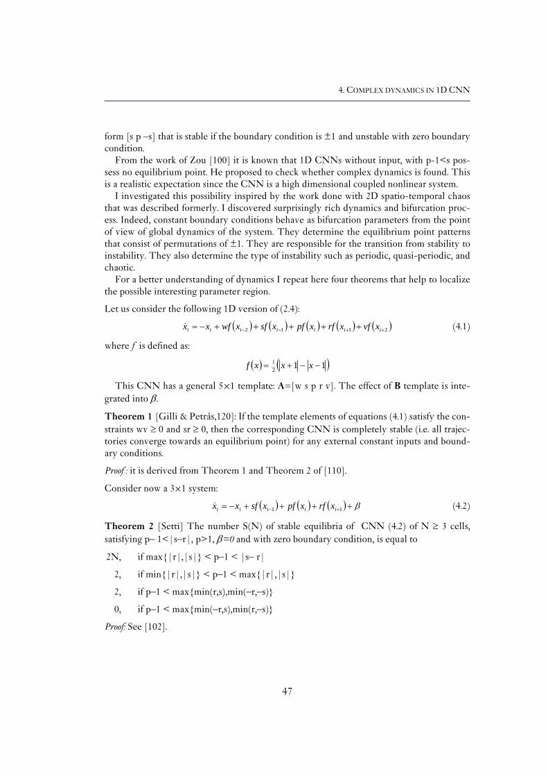
4. COMPLEX DYNAMICS IN 1D CNN
form [s p –s] that is stable if the boundary condition is ±1 and unstable with zero boundary condition.
From the work of Zou [100] it is known that 1D CNNs without input, with p-1<s pos-sess no equilibrium point. He proposed to check whether complex dynamics is found. This is a realistic expectation since the CNN is a high dimensional coupled nonlinear system.
I investigated this possibility inspired by the work done with 2D spatio-temporal chaos that was described formerly. I discovered surprisingly rich dynamics and bifurcation proc-ess. Indeed, constant boundary conditions behave as bifurcation parameters from the point of view of global dynamics of the system. They determine the equilibrium point patterns that consist of permutations of ±1. They are responsible for the transition from stability to instability. They also determine the type of instability such as periodic, quasi-periodic, and chaotic.
For a better understanding of dynamics I repeat here four theorems that help to localize the possible interesting parameter region.
Let us consider the following 1D version of (2.4):
( ) ( ) ( ) ( ) ( )2112 ++−− +++++−= iiiiiii xvfxrfxpfxsfxwfxx& (4.1)
where f is defined as:
( ) ( )1121 −−+= xxxf
This CNN has a general 5×1 template: A=[w s p r v]. The effect of B template is inte-grated into β.
Theorem 1 [Gilli & Petrás,120]: If the template elements of equations (4.1) satisfy the con-straints wv ≥ 0 and sr ≥ 0, then the corresponding CNN is completely stable (i.e. all trajec-tories converge towards an equilibrium point) for any external constant inputs and bound-ary conditions.
Proof : it is derived from Theorem 1 and Theorem 2 of [110].
Consider now a 3×1 system:
( ) ( ) ( ) β++++−= +− 11 iiiii xrfxpfxsfxx& (4.2)
Theorem 2 [Setti] The number S(N) of stable equilibria of CNN (4.2) of N ≥ 3 cells, satisfying p– 1<|s–r|, p>1, β=0 and with zero boundary condition, is equal to
2N, if max{|r|,|s|} < p–1 < |s– r|
2, if min{|r|,|s|} < p–1 < max{|r|,|s|}
2, if p–1 < max{min(r,s),min(–r,–s)}
0, if p–1 < max{min(–r,s),min(r,–s)}
Proof: See [102].
47

4. COMPLEX DYNAMICS IN 1D CNN
Theorem 3 [Zou] The CNN described in (4.2) with p>1, s>0 has no stable equilibrium point, if
β=0 and s>p–1
Proof: See [100].
Theorem 4 [Zou] The system defined by (4.2) with p>1, s>0 is completely stable if
β=0 and s<(p–1)/2
Proof: See [100].
These theorems restrict the possible parameter space of complex dynamics. Without loss of generality suppose that s > r. Summarizing the theorems yields that the following should be fulfilled so as the system does not have any stable equilibrium points:
s⋅r<0 (Theorem 1)
p–1 < |s–r|, p–1 < min{s,–r} (Theorem 2)
if s=–r, p–1 < s (Theorem 3)
I show that if the template parameters fulfill s > p–1 derived from these inequalities the boundary conditions behave as bifurcation parameters.
For the sake of simplicity I chose a one-dimensional opposite sign template class as a case study:
A=[s p –s].
For practical and theoretical reasons the dimension of the system under study is from four by one to eight by one.
Table 10 shows the possible equilibrium point patterns in a compact, regular expression form as a function of p, s and boundary conditions. They are composed of sequences of {+1,–1}. The string expression {a, b}0 represents the null string, whereas the expression {a, b}n denotes a string obtained by repeating n times the symbols a and b, e.g. {a, b}3 = a, b, a, b, a, b. The expressions were obtained using Deterministic Finite Automaton (DFA).
The possible stable equilibrium patterns of a CNN are represented in such a way that a stable pattern constitutes one node of a graph (see Fig. 49). The stability of a pattern around a cell is determined by the actual state of that cell and by its one or two neighbors. A cell has one neighbor, if it is a left– or rightmost cell and two neighbors if it is an inner cell. The nodes are organized into three columns. In the first column there are the stable patterns for the leftmost cells. On their left is a constant cell state of which is always equal to the left boundary condition. In the second (inner) column are the stable patterns for the inner cells. The third column contains the stable patterns for the rightmost cells. Their right neighbor is a constant cell with the right boundary condition.
48
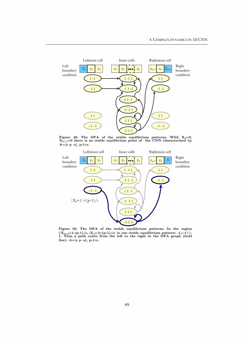
4. COMPLEX DYNAMICS IN 1D CNN
xn x2 xn-1x1 X0 Xn+1 x2
1 -1 1
-1 1 -1
1 1 -1
-1 -1 1
1 1 1
-1-1-1
1 -1
-1 1
1 1
-1 -1
1 1
–1 –1
1 1
–1 –1
Leftmost cell Inner cells Rightmost cell
x1 xn Left boundary condition
Right boundary condition
Figure 49. The DFA of the stable equilibrium patterns. With X0=0, XN+1=0 there is no stable equilibrium point of the CNN characterized by
A=[s p -s], p-1<s.
xn x2 xn-1x1 X0 0 x2
1 -1 1
-1 1 -1
1 1 -1
-1 -1 1
1 1 1
-1-1-1
1 -1
-1 1
1 1
-1 -1
–1 –1
Lefttmost cell Inner cells Rightmost cell
x1 xn Left boundary condition
Right boundary condition
|X0+1|<(p–1)/s
Figure 50. The DFA of the stable equilibrium patterns. In the region
{|XN+1|<1-(p-1)/s, |X0+1|<(p-1)/s} is one stable equilibrium pattern: -1,{-1}n,-1. Thus a path exists from the left to the right in the DFA graph (bold
line). A=[s p -s], p-1<s.
49

50
Equi
libri
um p
oint
pa
ttern
s X
N+
1 < –
(p –
1+
s)s
|X
N+
1+1|
< p
– 1
s
|X N
+1|
< –(
p –
1)+
ss
|X
N+
1 – 1
| <
p –
1s
X
N+
1 > p
– 1
+s
s
X0 <
– (p
– 1
+s)
s
–1,{
–1}n
,+1,
–1,{
+1,
–1}m
,+1
–1,{
–1}n
,+1
–1,{
–1}n
,+1,
–1,{
+1,
–1}m
,+1
–1,{
–1}n
,+1
–1,{
–1}n
,–1
–1,{
–1}n
,–1
–1,{
–1}n
,+1,
{–1,
+1}
m,–
1 –1
,{–1
}n,–
1 –1
,{–1
}n,+
1,{–
1,+
1}m
,–1
–1,{
–1}n
,–1
|X0+
1| <
p –
1s
–1
,{–1
}n,+
1,–1
,{+
1,–1
}m,+
1 +
1,–1
,{+
1,–1
}n,+
1 –1
,{–1
}n,+
1
–1,{
–1}n
,+1,
{–1,
+1}
m,–
1 +
1,–1
,+1,
{–1,
+1}
n,–
1 –1
,{–1
}n,–
1 –1
,{–1
}n,–
1 +
1,–1
,+1,
{–1,
+1}
m,–
1 –1
,+1,
{–1,
+1}
n,–
1 +
1,–1
,+1,
{–1,
+1}
n,–
1 –1
,+1,
{–1,
+1}
n,–
1
|X0|
< –
(p –
1)+
ss
–1
,+1,
–1,{
+1,
–1}n
,+1
+1,
–1,{
+1,
–1}n
,+1
–1,+
1,–1
,{+
1,–1
}n,+
1 +
1,–1
,{+
1,–1
}n,+
1 N
o equ
ilibr
ium
poi
nts
–1,–
1,+
1,{–
1,+
1}n,–
1 –1
,{–1
}n,–
1 –1
,{–1
}n,+
1,{–
1,+
1}m
,–1
–1,{
–1}m
,–1
|X0 –
1|
< p
– 1
s
+1,
{+1}
n,–
1,{+
1,–1
}m,+
1 –1
,+1,
–1,{
+1,
–1}n
,+1
+1,
{+1}
n,+
1
+1,
{+1}
n,–
1,{+
1,–1
}m,+
1 –1
,+1,
–1,{
+1,
–1}n
,+1
+1,
{+1}
n,+
1 +
1,{+
1}n,+
1
+1,
{+1}
n,–
1,+
1,{–
1,+
1}m
,–1
–1,+
1,{–
1,+
1}n,–
1 +
1,{+
1}n,–
1 +
1,{+
1}n,+
1
+1,
{+1}
n,–
1,+
1,{–
1,+
1}m
,–1
–1,+
1,{–
1,+
1}n,–
1 +
1,{+
1}n,–
1
X0 >
p –
1+
ss
+
1,{+
1}n,–
1,{+
1,–1
}m,+
1 +
1,{+
1}n,+
1 +
1,{+
1}n,–
1,{+
1,–1
}m,+
1 +
1,{+
1}n,+
1 +
1,{+
1}n,+
1 +
1,{+
1}n,–
1,+
1,{–
1,+
1}m
,–1
+1,
{+1}
n,–
1 +
1,{+
1}n,+
1
+1,
{+1}
n,–
1,+
1,{–
1,+
1}m
,–1
+1,
{+1}
n,–
1
Table
10.
The T
able
reports
a com
pact
express
ion fo
r all th
e poss
ible
st
able
equilib
riu
m poin
t patt
erns
in a C
NN
com
pose
d by N
cells
and
desc
rib
ed b
y a
1D
tem
pla
te [s,
p, -s
] (p
- 1
< s
and s
> 0
) w
ith b
oundary c
ondit
ions
X0 a
nd X
N+
1 . T
he p
att
erns
have b
een d
ete
rm
ined b
y e
x-
plo
itin
g a
rig
orous
techniq
ue, base
d o
n D
FA
(D
ete
rm
inis
tic F
init
e A
uto
mata
). T
he t
wo p
aram
ete
rs
n a
nd m
are n
onnegati
ve inte
ger n
um
bers.
The s
trin
g e
xpress
ion {
a, b
}0 r
eprese
nt
the n
ull s
trin
g, w
hereas
the e
xpress
ion {
a, b
}n d
enote
s a s
trin
g o
bta
ined b
y r
epeati
ng n
tim
es
the s
ym
-
bols
a a
nd b
, e.g
. { a
, b
}3 =
a, b, a, b, a, b.

4. COMPLEX DYNAMICS IN 1D CNN
Definition. Oriented connection exists between two nodes if the second node is the con-tinuation of the first node. This means that the two-element vector formed from the two rightmost elements of the first node and the two-element vector formed from the two left-most elements of the second (inner) node are the same (Fig. 49). Formally: Oriented connection exists between two nodes: n1→n2
n1={S1,S2,S3,}and n2={Q1,Q2,Q3,} iff. S2=Q1 and S3=Q2 , where Si ,Qi ∈ {–1,1}. (Inner Node) n1={X0,L2,L3,}and n2={S1,S2,S3,} iff. L2=S1 and L3=S2 , where Li ,Si ∈ {–1,1}. (Left Node) n1={S1,S2,S3,}and n2={R1,R2,R3,} iff. S2=R1 and S3=R2 , where Si ,Ri ∈ {–1,1}. (Right Node)
Definition. A path is a sequence of connections. A pattern is a stable equilibrium point if a path exists from a node in the first column to a
node in the last column (Fig. 50). Using this graph based rigorous technique all the stable equilibrium patterns can be
represented as directed paths. It is revealed that the parameter space can be divided into twenty-five sub-regions. Except the central unstable region {|X0|<1–(p–1)/s, |XN+1|<1–(p–1)/s} all the sub-regions exhibit at least one stable equilibrium point.
This central unstable region is the most probable parameter sub-space for finding com-plex behaviour. However, it cannot be excluded that in the regions with one or more stable equilibrium points are other attractors such as limit cycles or chaotic attractors. In fact, later I will show that this is the case.
-0.04
-0.03
-0.02
-0.01
0
0.01
0.02
0.03
0.04
X0
Xn+1
-1 -0.5 0 0.5 1
-1
-0.5
0
0.5
1
Figure 51. The parameter space of a 4x1 CNN with A=[0.9 1.1 -0.9]. Yellow to red colors mean positive Lyapunov exponents, green means two zero exponents (torus or quasi-periodic dynam-ics), blue denotes periodic behaviour with single zero exponent as the greatest one. White means stable region with all expo-nents being zero.
51

4. COMPLEX DYNAMICS IN 1D CNN
4.2 Nonlinear dynamics
4.2.1 Study of 1D CNN with a selected template
I used first order 1D CNN with linear templates (2.4). I considered the following sign anti-symmetric template without any input:
A=[ 0.9 1.1 –0.9 ]
-1.1 -1 -0.9 -0.8 -1
-0.9
-0.8
-0.7
x 2
x1
x 0 = -0.75, xn+1 = -0.95
-1 -0.5 0 0.5 1
-0.5
0
0.5
1
1.5
x 2
x1
x0= 0.376, xn+1= -0.197
-1 0 1
-1
-0.5
0
0.5
1
x 2 x
1
x0= 0.025, xn+1= 0.25
-1.5 -1 -0.5 -0.8 -0.6 -0.4 -0.2
0 0.2
x 2
x 1
x 0 = -0.4, x n+1 = -0.85
-1.2 -1 -0.8 -0.6 0.2 0.4 0.6 0.8
1
x 2
x 1
x 0 = 0.575, x n+1 = -0.75
X 0
Xn+1
-1 -0.8 -0.6 -0.4 -0.2 0 0.2 0.4 0.6 0.8 1
-1
-0.8
-0.6
-0.4
-0.2
0
0.2
0.4
0.6
0.8
1
-0.5 0 0.5 1 1.5 -1
-0.5
0
0.5
1x 2
x 1
x0= 0.1, x n+1 = 0.15
0 0.5 1
0
0.5
1
1.5
x 2
x 1
x0= 0.6, x n+1 = 0.4
-1.2 -1 -0.8 -0.6
0.4
0.6
0.8
1
x 2
x1
x 0 = 0.7, xn+1= -0.75
-1 -0.5 0-0.5
0
0.5
1
x 2
x1
x0= 0.425, xn+1= -0.4
-1 0 1
-1
-0.5
0
0.5
1
1.5
x 2
x1
x0= 0.2, xn+1= 0.025
LE: 0.022
LE: 0.037
LE: 0.039
LE: 0.062
Figure 52. Lyapunov map of a 4x1 CNN with A=[0.9 1.1 -0.9]. Some observed attrac-tors are shown. Color code. Yellow-red: chaotic attractor; green: torus (quasi-periodic); blue: limit cycle (periodic); white: equilibrium point.
52
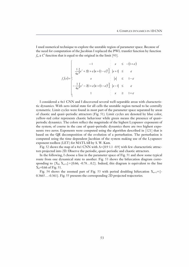
4. COMPLEX DYNAMICS IN 1D CNN
I used numerical technique to explore the unstable region of parameter space. Because of the need for computation of the Jacobian I replaced the PWL transfer function by function fε, a C1 function that is equal to the original in the limit [93].
( )
( )
( ) ( )[ ]
( ) ( )[ ]⎪⎪⎪⎪⎪
⎩
⎪⎪⎪⎪⎪
⎨
⎧
+≥
≤−−++−−
−≤
≤+−+++
+−≤−
=
ε
εεεε
ε
εεεε
ε
ε
11
111241
1
111241
11
22
22
x
xxx
xx
xxx
x
xf
I considered a 4x1 CNN and I discovered several well-separable areas with characteris-tic dynamics. With zero initial state for all cells the unstable region turned to be centrally symmetric. Limit cycles were found in most part of the parameter space separated by areas of chaotic and quasi–periodic attractors (Fig. 51). Limit cycles are denoted by blue color, yellow-red color represents chaotic behaviour while green means the presence of quasi–periodic dynamics. The colors reflect the magnitude of the highest Lyapunov exponents of the system; of course in the case of quasi–periodic dynamics there are two highest expo-nents: two zeros. Exponents were computed using the algorithm described in [121] that is based on the QR decomposition of the evolution of a perturbation. The perturbation is computed using the time dependent Jacobian of the system making use of the Lyapunov exponent toolbox (LET) for MATLAB by S. W. Kam.
Fig. 52 shows the map of a 4x1 CNN with A=[0.9 1.1 -0.9] with few characteristic attrac-tors projected into 2D. Observe the periodic, quasi-periodic and chaotic attractors.
In the following, I choose a line in the parameter space of Fig. 51 and show some typical route from one dynamical state to another. Fig. 53 shows the bifurcation diagram corre-sponding to {X0; Xn+1}={0.66; -0.78…0.2}. Indeed, this diagram is equivalent to the line X0=0.66 of Fig. 51.
Fig. 54 shows the zoomed part of Fig. 53 with period doubling bifurcation Xn+1={-0.3665…-0.361}. Fig. 55 presents the corresponding 2D projected trajectories.
53
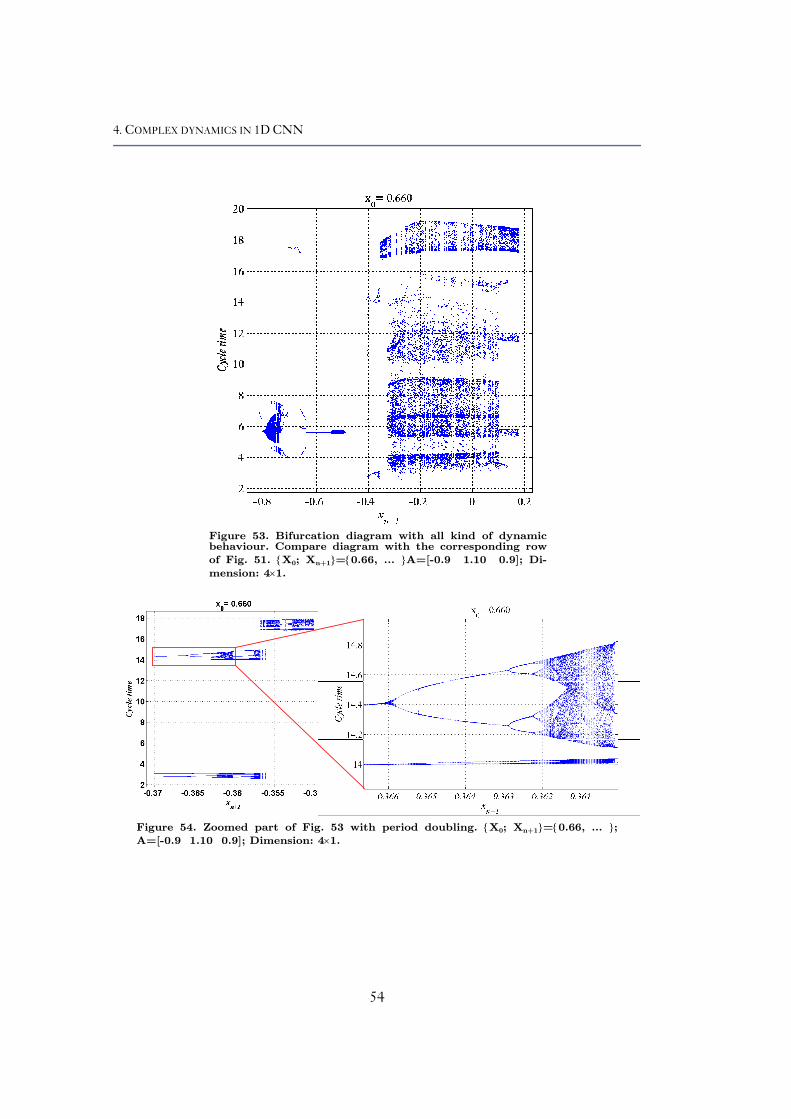
4. COMPLEX DYNAMICS IN 1D CNN
Figure 53. Bifurcation diagram with all kind of dynamic behaviour. Compare diagram with the corresponding row
of Fig. 51. {X0; Xn+1}={0.66, ... }A=[-0.9 1.10 0.9]; Di-
mension: 4×1.
Figure 54. Zoomed part of Fig. 53 with period doubling. {X0; Xn+1}={0.66, ... }; A=[-0.9 1.10 0.9]; Dimension: 4×1.
54
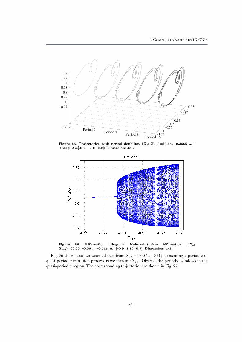
4. COMPLEX DYNAMICS IN 1D CNN
Period 1Period 2
Period 4Period 8
Period 16-1.25
-1-0.75
-0.5-0.25
00.25
0.50.75-0.25
00.25
0.50.75
11.25
1.5
Figure 55. Trajectories with period doubling. {X0; Xn+1}={0.66, -0.3665 ... -
0.361}; A=[-0.9 1.10 0.9]; Dimension: 4×1.
Figure 56. Bifurcation diagram. Naimark-Sacker bifurcation. {X0;
Xn+1}={0.66, −0.56 ... −0.51}; A=[−0.9 1.10 0.9]; Dimension: 4×1.
Fig. 56 shows another zoomed part from Xn+1={-0.56…-0.51} presenting a periodic to quasi-periodic transition process as we increase Xn+1. Observe the periodic windows in the quasi-periodic region. The corresponding trajectories are shown in Fig. 57.
55

4. COMPLEX DYNAMICS IN 1D CNN
-0.546 -0.545 -0.544 -0.543 -0.542 -0.541 -0.54 -0.539 -0.538-1.1
-1-0.9
-0.8-0.7
-0.6-0.5
-0.4-0.3
-0.2-0.1-0.2
00.20.40.60.8
11.21.4
Figure 57. Trajectories of limit cycle to torus transition. {X0; Xn+1}={0.66, -0.546...-0.538}; A=[-0.9 1.10 0.9]; Dimension: 4×1.
Xn+1
Figure 58. Bifurcation diagram. Alternating Torus-Chaos windows. {X0; Xn+1}={0.66, ...}; A=[-0.9 1.10 0.9]; Dimension: 4×1.
56

4. COMPLEX DYNAMICS IN 1D CNN
Figure 59. Bifurcation diagram. Torus-Chaos win-
dows - zoomed region. {X0; Xn+1}={0.66, ...}; A=[-0.9
1.10 0.9]; Dimension: 4×1.
Fig. 58 presents a region of the bifurcation diagram of Fig. 53 in which periodic, quasi-periodic and chaotic regions are alternating. Fig. 59 shows a zoomed part in which torus-chaos transition is shown. Some corresponding trajectories are presented in Fig. 60. Fig. 61 shows the 2D projection of Poincare map of a quasi-periodic attractor of the 4×1 CNN with A=[-0.9 1.10 0.9] at {X0; Xn+1}={0.66,-0.53}.
-0.76 -0.7595-0.759-0.7585-0.758-0.7575-0.757-1.3-1.2
-1.1-1
-0.9-0.8
-0.7-0.6
-0.50.20.30.40.50.60.70.80.9
11.1
Xn+1
Figure 60. Torus to Chaos transition. Trajectories. {X0; Xn+1}={0.66, -0.76...-
0.757}; A=[-0.9 1.10 0.9]; Dimension: 4×1.
57

4. COMPLEX DYNAMICS IN 1D CNN
Figure 61. 2D projection of the Poincare map of a torus at {X0;
Xn+1}={0.66,-0.53}; A=[-0.9 1.10 0.9]; Dimension: 4×1.
Figure 62. The ”Brain”. 2D projection of the Poincare map of
four cell CNN at {X0; Xn+1}={-0.867,-0.463}; A=[-0.9 1.10 0.9];
Dimension: 4×1.
58

4. COMPLEX DYNAMICS IN 1D CNN
Figure 63. Zoomed part of the Brain map. Observe the fractal
structure.{X0; Xn+1}={-0.867,-0.463}; A=[-0.9 1.10 0.9]; Dimen-
sion: 4×1.
Fig 62 and 63 show the 2D projection of the first return map of the 4×1 CNN with A=[-0.9 1.10 0.9] at {X0; Xn+1}={-0.867,-0.463}.
59

4. COMPLEX DYNAMICS IN 1D CNN
Sub thesis II/b.
Chaotic dynamics, coexistence of attractors in 1D CNN
I uncovered novel complex dynamics in 1D CNNs with a sign-antisymmetric tem-plate class. I investigated the effect of the boundary condition, dimension of the system and initial state. I found that boundary condition behaves as bifurcation parameter. I found coexistence of attractors depending on the initial state.
II/b. Effect of dimension and initial sate, coexistence of attractors I showed that the steady state dynamics depends on the initial state: attractors coexist simultane-ously in the same system. I showed that hyperchaotic behavior can occur in a CNN that consist of more than five cells. I demonstrated that the parity of the size of the 1D system drastically changes the dynamics.
4.2.2 Coexistence of attractors in a 4×1 CNN
Perhaps the most important result in this thesis is the simultaneous existence of different attractors. This could be exploited by further research for e.g information storage.
As I noted before the existence of stable equilibrium points does not necessarily exclude the presence of other types of attractors. Indeed, in regions
a) { ( ) spsX +−−< 10 , 111 −<++ psX N }
b) { 110 −<+ psX , ( ) spsX N +−−<+ 11 }
c) { ( ) spsX +−−< 10 , 111 −<−+ psX N }
d) { 110 −<− psX , ( ) spsX N +−−<+ 11 }
I found the coexistence of stable equilibrium points, limit cycles and chaotic attractors that are another example to that of the authors in section V. of [122].
The presence of different attractors is also valid in the unstable region {|X0|<1–(p–1)/s, |XN+1|<1–(p–1)/s}.
60
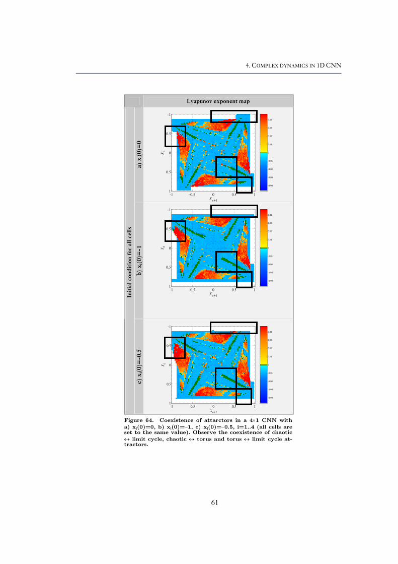
4. COMPLEX DYNAMICS IN 1D CNN
Lyapunov exponent map
a) x
i(0)=
0
-0.04
-0.03
-0.02
-0.01
0
0.01
0.02
0.03
0.04
X0
Xn+1
-1 -0.5 0 0.5 1
-1
-0.5
0
0.5
1
b) x
i(0)=
-1
-0.04
-0.03
-0.02
-0.01
0
0.01
0.02
0.03
0.04
X0
Xn+1
-1 -0.5 0 0.5 1
-1
-0.5
0
0.5
1
Init
ial c
ondi
tion
for
all c
ells
c)
xi(0
)=-0
.5
-0.04
-0.03
-0.02
-0.01
0
0.01
0.02
0.03
0.04
X0
Xn+1
-1 -0.5 0 0.5 1
-1
-0.5
0
0.5
1
Figure 64. Coexistence of attarctors in a 4×1 CNN with
a) xi(0)=0, b) xi(0)=−1, c) xi(0)=−0.5, i=1..4 (all cells are set to the same value). Observe the coexistence of chaotic
↔ limit cycle, chaotic ↔ torus and torus ↔ limit cycle at-tractors.
61
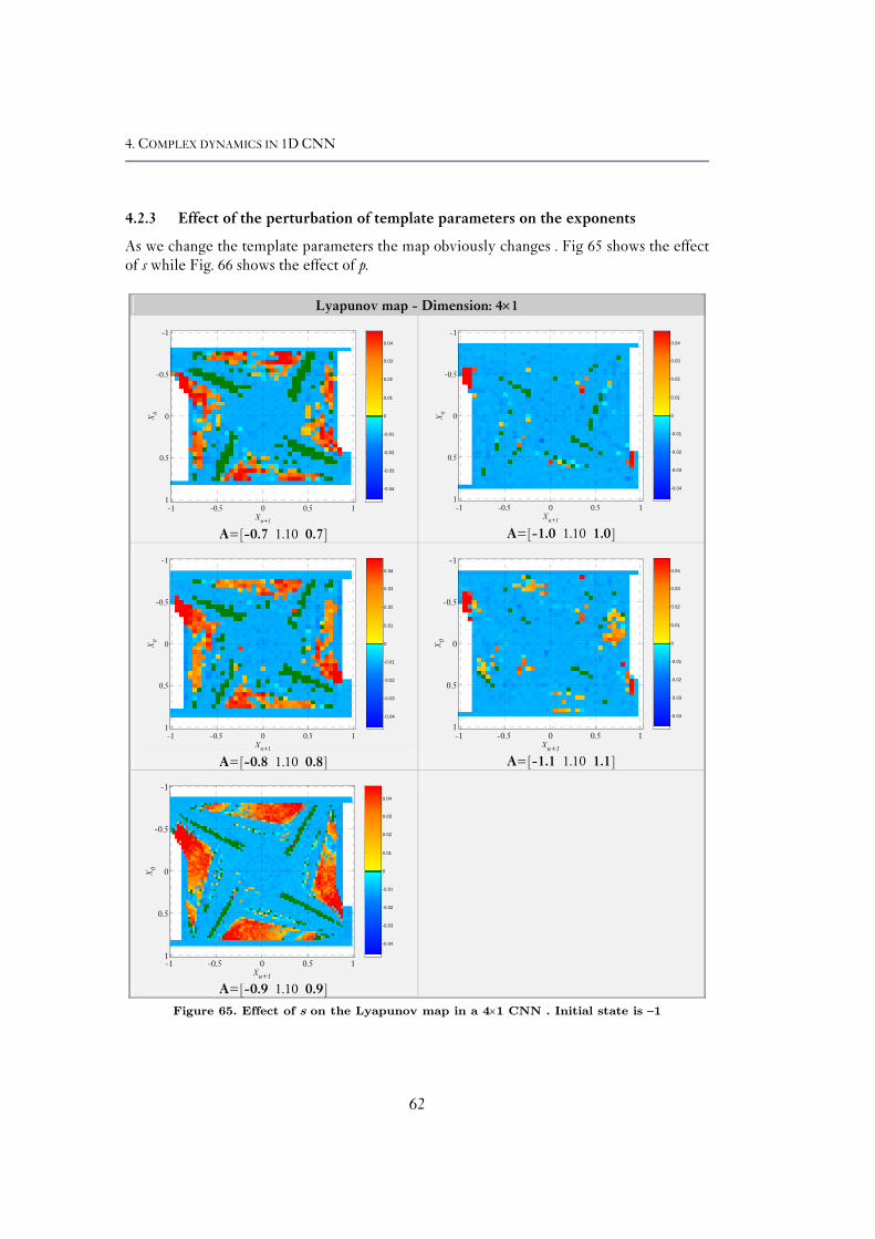
4. COMPLEX DYNAMICS IN 1D CNN
4.2.3 Effect of the perturbation of template parameters on the exponents
As we change the template parameters the map obviously changes . Fig 65 shows the effect of s while Fig. 66 shows the effect of p.
Lyapunov map - Dimension: 4×1
-0.04
-0.03
-0.02
-0.01
0
0.01
0.02
0.03
0.04
X0
X-1 -0.5 0 0.5 1
-1
-0.5
0
0.5
1
n+1
A=[-0.7 1.10 0.7]
-0.04
-0.03
-0.02
-0.01
0
0.01
0.02
0.03
0.04
X0
Xn+1
-1 -0.5 0 0.5 1
-1
-0.5
0
0.5
1
A=[-1.0 1.10 1.0]
-0.04
-0.03
-0.02
-0.01
0
0.01
0.02
0.03
0.04
X0
Xn+1
-1 -0.5 0 0.5 1
-1
-0.5
0
0.5
1
A=[-0.8 1.10 0.8]
-0.04
-0.03
-0.02
-0.01
0
0.01
0.02
0.03
0.04
X0
X-1 -0.5 0 0.5 1
-1
-0.5
0
0.5
1
n+1 A=[-1.1 1.10 1.1]
-0.04
-0.03
-0.02
-0.01
0
0.01
0.02
0.03
0.04
X0
Xn+1
-1 -0.5 0 0.5 1
-1
-0.5
0
0.5
1
A=[-0.9 1.10 0.9]
Figure 65. Effect of s on the Lyapunov map in a 4×1 CNN . Initial state is −1
62

4. COMPLEX DYNAMICS IN 1D CNN
Lyapunov map - Dimension: 4×1
-0.04
-0.03
-0.02
-0.01
0
0.01
0.02
0.03
0.04
X0
X-1 -0.5 0 0.5 1
-1
-0.5
0
0.5
1-0.04
-0.03
-0.02
-0.01
0
0.01
0.02
0.03
0.04
X0
X-1 -0.5 0 0.5 1
-1
-0.5
0
0.5
1
n+1n+1
A=[-0.9 1.05 0.9] A=[-0.9 1.20 0.9]
-0.04
-0.03
-0.02
-0.01
0
0.01
0.02
0.03
0.04
X0
X-1 -0.5 0 0.5 1
-1
-0.5
0
0.5
1
n+1
A=[-0.9 1.10 0.9] A=[-0.9 1.25 0.9]
-0.04
-0.03
-0.02
-0.01
0
0.01
0.02
0.03
0.04
X0
X-1 -0.5 0 0.5 1
-1
-0.5
0
0.5
1-0.04
-0.03
-0.02
-0.01
0
0.01
0.02
0.03
0.04
X0
Xn+1
-1 -0.5 0 0.5 1
-1
-0.5
0
0.5
1
n+1
A=[-0.9 1.15 0.9] A=[-0.9 1.30 0.9] Figure 66. Effect of p on the Lyapunov map in a 4×1 CNN .
4.2.4 Higher dimension - Hyperchaos
I showed that hyperchaotic behaviour can occur even in a 6x1 size CNN. Hyperchaos means that the system has more than one positive Lyapunov exponents.
63

4. COMPLEX DYNAMICS IN 1D CNN
Lyapunov exponents - A=[-0.9 1.10 0.9]
-0.04
-0.03
-0.02
-0.01
0
0.01
0.02
0.03
0.04
X0
Xn+1
-0.5 0 0.5
-0.8
-0.6
-0.4
-0.2
0
0.2
0.4
0.6
0.8
Dimension: 3×1
-0.04
-0.03
-0.02
-0.01
0
0.01
0.02
0.03
0.04
X0
Xn+1
-1 -0.5 0 0.5 1
-1
-0.5
0
0.5
1
Dimension: 4×1
-0.04
-0.03
-0.02
-0.01
0
0.01
0.02
0.03
0.04
X0
Xn+1
-0.5 0 0.5
-0.8
-0.6
-0.4
-0.2
0
0.2
0.4
0.6
0.8
Dimension: 5×1
-0.04
-0.03
-0.02
-0.01
0
0.01
0.02
0.03
0.04
X0
Xn+1
-0.5 0 0.5
-0.8
-0.6
-0.4
-0.2
0
0.2
0.4
0.6
0.8
Dimension: 6×1
-0.04
-0.03
-0.02
-0.01
0
0.01
0.02
0.03
0.04
X0
Xn+1
-0.5 0 0.5
-0.8
-0.6
-0.4
-0.2
0
0.2
0.4
0.6
0.8
Dimension: 7×1
-0.04
-0.03
-0.02
-0.01
0
0.01
0.02
0.03
0.04
X0
Xn+1
-0.5 0 0.5
-0.8
-0.6
-0.4
-0.2
0
0.2
0.4
0.6
0.8
Dimension: 8×1
Figure 67. Effect of the dimension of the CNN on the Lyapunov map. Dimensions of the
CNN are from 3×1 to 8×1. A=[-0.9 1.10 0.9]
This can only appear in dynamical systems having dimension N>3. In the case of CNN the presence of hyperchaos was found with N≥6. Fig. 67 shows the effect of the size of the system on the dynamics.
64

4. COMPLEX DYNAMICS IN 1D CNN
Chaos (yellow-red) Number of positive exponents
-0.04
-0.03
-0.02
-0.01
0
0.01
0.02
0.03
0.04
X0
Xn+1
-0.5 0 0.5
-0.8
-0.6
-0.4
-0.2
0
0.2
0.4
0.6
0.8 0
0.5
1
1.5
2
2.5
3
X0
Xn+1
-0.5 0 0.5
-0.8
-0.6
-0.4
-0.2
0
0.2
0.4
0.6
0.8
Dimension: 6×1
-0.04
-0.03
-0.02
-0.01
0
0.01
0.02
0.03
0.04
X0
Xn+1
-0.5 0 0.5
-0.8
-0.6
-0.4
-0.2
0
0.2
0.4
0.6
0.8
Dimension: 7×1
0
0.5
1
1.5
2
2.5
3
X0
Xn+1
-0.5 0 0.5
-0.8
-0.6
-0.4
-0.2
0
0.2
0.4
0.6
0.8
-0.04
-0.03
-0.02
-0.01
0
0.01
0.02
0.03
0.04
X0
Xn+1
-0.5 0 0.5
-0.8
-0.6
-0.4
-0.2
0
0.2
0.4
0.6
0.8
Dimension: 8×1
0
0.5
1
1.5
2
2.5
3
X0
Xn+1
-0.5 0 0.5
-0.8
-0.6
-0.4
-0.2
0
0.2
0.4
0.6
0.8
Figure 68. Hyperchaos in 6×1, 7×1 and 8×1 CNNs. In the right column the color denotes the number of positive Lyapunov exponents.
Observe that parity of the number of cells can play an important role. Maps of the sys-tems having the same parity of number of cells are similar. Fig. 68 shows the systems that
65

4. COMPLEX DYNAMICS IN 1D CNN
exhibit more than one positive Lyapunov exponents. The color-coded number of positive exponents are shown in the right column.
66

4. COMPLEX DYNAMICS IN 1D CNN
67


5. SPECIAL WAVE OPERATOR
5. Special wave operator
Third Thesis
Curvature controlled trigger wave
I showed that the CNN with a nonlinear diffusion type template class computes the approximation of the so–called “Curve Shortening Flow” of shapes. Indeed, the process can be described as local curvature controlled trigger wave propagation in the CNN array. In this framework the curve is represented as the boundary region of a solid black shape against white background. As a result of the diffusion–like evolution of the CNN array, a smooth 2D transition zone called boundary region is formed between black and white regions. The width of the region is controlled by the template parameters. The evolution of the shape of this region corresponds to the evolution of the curve. To show this, at first I analyzed the characteristics of the boundary region of the evolving shape than I studied the dynamics of this transition region.
III/a. Stability of the boundary I proved that the boundary region is stationary provided that the region is horizontal or vertical. I gave relation on the number of linear cells in a horizontal or vertical boundary region. I gave approximation on the minimal number of linear cells of arbitrary oriented straight boundaries.
69
5. SPECIAL WAVE OPERATOR
III/b. Dynamics of the boundary region I showed that the temporal derivative of the state variable of a linear cell being in the boundary region is the quasi-linear function of the local curvature of the isointensity line to which the cell belongs provided that the state variable of the cell is close to zero. This is fulfilled in the centerline of the boundary region. The boundary region changes so that its local curvature is zero. In other words the shape contours get smoothed provided that spatial constraints make this possible. I gave method to compute the convex hull of a shape in one transient. Moreover, I gave method to sepa-rate two-dimensional clusters of points.
onlinear (active) waves are natural phenomena that can be found everywhere around us in Nature and described by various fields of sciences. They can be ob-
served in e.g. chemistry [4], or biology [28,29]. Their basic property is that the wave propagates in an excitable (bistable) medium in a way that a small unit of the medium tran-sits from one stable state to another at the expense of energy stored in the medium. The transition triggers the local neighborhood thus the propagation is self-sustaining; from here comes the name: auto(nomous)-wave (R. V. Khorhlov). Such nonlinear active waves are autowaves 31 (traveling waves, trigger waves, target (or concentric) waves [4]) and spiral waves [29].
n
Due to their local dynamics nature, considering continuous descriptions in space and time, reaction-diffusion PDEs are the plausible mathematical models for these phenomena.
PDEs have proved to be useful as a general framework for image processing [32,33]. Multiscale analysis originally based on linear PDE filters [34]; later nonlinear diffusion filters were developed to avoid the artifacts [35-38]. In the active contour (or snakes) ap-proach for object detection the contour propagation is also governed by PDEs [39,40]. In the level-set approach a PDE controls the evolution of a set of isointensity contours of the image [41,42].
Till now this field remained a focused and intensive research area. Several works re-vealed the connection between the different PDE related image-processing methods [32,43-45].
The main drawback of the approach is the increased computing power requirement be-cause of the need of the numerical solution of PDEs. With parallel computing architecture this requirement can be overcome. This implies spatial discretization that gives an ap-proximation of the original PDE. However with an appropriate spatial constant the original dynamics can be reproduced. Thus the PDE dynamics is described by a set of ODEs.
For parallel computing of PDEs obviously we need programmable processors. However, they do not need to be as complex and general as a microprocessor or DSP. It is sufficient if they can ‘only’ compute ODEs. At first sight this might seem to make no sense, however considering analog implementation this approach shows itself much more attractive.
70

5. SPECIAL WAVE OPERATOR
A suitable computing model that is hardware feasible can be the Cellular Nonlinear Networks [46-49] introduced in Chapter 2. The most widely applied variant of it consists of first order nonlinear dynamical systems that are locally coupled and organized into a two-dimensional array. An intensive research has recently emerged in the CNN field. Sev-eral linear, nonlinear filtering methods and wave computing algorithms were developed [56,64-74]. The structure of the CNN naturally makes it a possible tool as spatially discre-tized PDE computer [75,76].
The CNN as an active medium has been studied extensively. Several types of nonlinear waves have been reproduced and analyzed on this structure depending on the complexity of the elementary cells [31,59,77-82].
5.1 Shape deformation
Recently several papers have dealt with the CNN as a wave-computing device [57,59,64,65,75,83,84]. It has been proved to be a suitable computing frame for wave-based image processing. Some of these algorithms used autowaves for specific tasks [74], others used trigger waves for some kind of morphological processing in which the shape is de-formed by the wave.
These trigger wave-based processes were one-way: if the spreading wave triggered a cell then it remained triggered [64]. However, using an appropriate nonlinear diffusion opera-tor this property can be violated yielding a qualitatively different behaviour [85].
Figure 69 Curve shortening flow
The phenomenon that is well-known from the image processing literature [167,168] is described by
( )
Nt
tlC rκ−=
∂∂ , (5.1)
where C is the boundary vector of coordinates (the planar curve), κ is the local curvature,
Nr
is the outward normal, l is the curve parameter, t is the scale parameter (Fig. 69). This equation is known as the geometric heat equation or curve shortening flow in differ-
ential geometry. Several work dealt with this flow (see for review e.g. [33]). It had been proved [86,87] that all closed contours collapse into a single point under this flow.
During the evolution of this flow the shape (closed contour) propagates along its out-ward normal direction and collapses under its curvature, which gives rise to obtain a hier-archy of shapes and thus a scale space for shapes can be formed [88-90]. These scale spaces
71

5. SPECIAL WAVE OPERATOR
and their enhancements gave a suitable framework for recognition, classification and re-trieval of shapes. Due to numerical and theoretical reasons Osher and Sethian proposed an approach in which the curve flow is embedded as the zero level set of a surface [42]. The surface is evolved by its mean curvature and due to the special shape of the surface the mean curvature of the surface corresponded to the curvature of the embedded curve at the zero level set and the evolution of the surface contained the evolution of the original curve. See [166] for on-line reference.
The CNN based nonlinear diffusion works similar way. The shape is given as the initial state of the array. The zero level set (or isointensity line) of the state is considered as the evolving contour of the shape during the evolution (see Fig. 70). Black (+1) color means “inside”, white means “outside” of the shape.
The boundary region of a shape is a one- or two-dimensional transition zone between opposite-signed saturated cells (1D) or between regions (2D; see Fig. 73, 75 and 79). The state variables of cells that constitute the boundary are in the linear part of transfer function (5.3) i.e. -1<xij<+1. Please do not to mistake boundary region for boundary condition of the CNN array in this thesis.
It will be shown that due to the flat shape1 of the boundary region (see Fig. 78) the mean curvature of the surface and the curvature of the embedded curve are practically the same. Therefore the boundary region evolves according to the curvature of the embedded shape.
Using the discretized version of the following nonlinear diffusion operator A( ). =D∇2f( ). +aef( ). the CNN computes the approximation of the curve shortening flow in one transient.
, (5.2) ( )∑ ∑−= −=
+++−=q
qk
q
qlljkiklijij txfAtxtx )()()( ,&
⎥⎥⎥
⎦
⎤
⎢⎢⎢
⎣
⎡−=
04/0
4/4/
04/0
D
DDaD
D
A e
where q =1, x is the state of the CNN, f = is a nonlinear transfer function [93] de-
fined by (5.3).
εε
f0
lim→
( )
( )
( ) ( )[ ]
( ) ( )[ ]⎪⎪⎪⎪⎪
⎩
⎪⎪⎪⎪⎪
⎨
⎧
+≥
≤−−++−−
−≤
≤+−+++
+−≤−
=
ε
εεεε
ε
εεεε
ε
ε
11
111241
1
111241
11
22
22
x
xxx
xx
xxx
x
xf
(5.3)
At the beginning of the evolution of the CNN the shape is implicitly embedded into a surface through the blurring of the diffusion process (Fig. 71). As a result, a linear transition
1 the linearity of the cross section of the surface along the gradient direction. This shape is a special characteristic of the CNN and maintained during the evolution.
72

5. SPECIAL WAVE OPERATOR
zone is formed between the black and white regions. Cells belonging to the zone are in the linear region of (5.3). Cells being black or white are said to be saturated. They are in the saturation region of (5.3). The width of the linear region can be influenced by parameters D and ae (Fig. 72). However the blur is spatially limited: the nonlinear character of the diffu-sion maintains the constant width and the gradient of the linear zone. This width is inde-pendent of the orientation and the shape of the zone throughout the transient. When the desired curve smoothing is reached the transient is stopped.
The CNN may be used as an effective parallel “curve shortening flow computer” and we can use the results developed for scale-spaces of shapes ([88-90]).
Out
put
time t: 0 Local curvature at t:1
t: 4 14 34
Figure 70. s=0.6,p=-1, boundary condition of the array is zeroflux
Figure 71. Linear zone of the interface between the black and white regions.
5.2 Number of linear cells
In this section I derive some relations on the boundary zone of the embedded shapes. At first I consider straight boundaries that are horizontal or vertical. In the second subsection boundaries are considered that are oriented along the π/4 direction. I derive a conjecture on the length of the linear zone along the gradient.
5.2.1 Horizontally or vertically aligned boundary region Several authors investigated one-dimensional CNNs. In [91] Thiran et al. proved that the stable pattern of a 1D CNN with p,s > 0, -1< (p-1)/2s <1 consists of a succession of alter-natively black and white pair of adjacent saturated cells, separated by boundaries of B lin-ear pixels. He gave conditions necessary for the stability of a pattern and also gave the range of stable patterns. This theorem can be easily extended into 2D CNN having hori-
73

5. SPECIAL WAVE OPERATOR
zontally or vertically oriented patterns (Fig 73). In 2D the linear cells form the boundary region between the black and white regions.
Stable pattern Stable pattern Unstable pattern Unstable pattern Stable pattern
initi
al st
ate
snap
shot
ae =2.39,
D=2.4 B1D=0
ae =2.39, D=2.4 B1D=0
ae =1.3, D=2.4 B1D=3
ae =1.06, D=2.4 B1D=8
ae=2.45, D=2.4 B1D=0
Figure 72. The effect of the self-feedback on the propagation; B1D is the number of linear cells.
B linear cells 5 10 15 20
-1
-0.5
0
0.5
1
Figure 73. Extension of 1D stable pattern into 2D. B=7
The following proposition shows the relation of the one- and two-dimensional stable pat-terns provided that in 2D the boundary regions are oriented vertically or horizontally (i.e. the gradient vector of the 2D image is parallel with or perpendicular to the x axis of the image respectively).
r s r s p s r s r
r s r s p s r s r
Figure 74. 2D vertically oriented boundary re-gions with and without linear cells. The dy-namics of all rows are the same.
74

5. SPECIAL WAVE OPERATOR
Proposition:
, (5.4) ( )∑ ∑−= −=
+++−=q
qk
q
qlljkiklijij (t)xfA(t)x(t)x ,&
⎥⎥⎥
⎦
⎤
⎢⎢⎢
⎣
⎡=
rsr
sps
rsr
A
where q=1. Let s, r > 0, p < 1, 4s + 4r + p > 1. Moreover, let the initial state of the infinite or periodic 2D CNN (5.4) consist of identical rows or columns (Fig. 74).
Then the one-dimensional equivalent CNN has the form
( ) ( ) ( )11 +− +++−= iiiii xfsxfpxfsxx )))& , [ ]sps )))=A (5.5)
pspsrs +=+= 2,2))
and the number of linear cells [91] in the boundary zone is an integer B:
( ) ( ) 1arccos
2arccos
−−
<<−− µπ
πµπ
πB where
sp)
)
21−
=µ (5.6)
Proof:
The dynamics of all rows are the same therefore the array can be written as a vector:
(5.7) ( ) ( ) ( ) ( ) ( ) ( 11
11
11
11
222 +−
+−
+−
+−
++++++−=⎪⎭
⎪⎬
⎫
iii
iii
iii
iii
xfsrxfpsxfsrxx
rxsxrx
sxpxsx
rxsxrx& )
Thus, the 2D array is transformed to 1D provided that the initial state is made up of black and (gray and) white regions separated by vertical regions. Doing so, we can use the theory from [91] for the number of linear cells equation (5.6). The same results are hold for horizontally aligned boundary regions as well.
5.2.2 Boundary region aligned with π/4
Let us consider an infinite 2D CNN controlled by template A. The governing equation is the same as in (5.4) with the following:
s > 0, p < 1, 4s+p > 1, (5.8) ⎥⎥⎥
⎦
⎤
⎢⎢⎢
⎣
⎡=
00
00
s
sps
s
A
To gain a relationship between p, s and B, I use a way of thinking similar to that of in [91] but I extend it into 2D with restrictions. Compared to the 1D case, the degree of free-dom of the parameters increases greatly. The number of possible stable patterns also in-creased a lot. Due to these only few things can be stated.
75

5. SPECIAL WAVE OPERATOR
In spite of the fact that the linear analysis is not valid for equation (5.4) it is still useful for deriving some results for the number of linear cells in 2D.
The two-dimensional discrete Fourier transform of the template matrix is:
(5.9) ( 21 coscos21][~ ωωω ++−= spA )
This describes the filtering characteristic of the CNN in the linear region.
Let 21 ωω = . This means that the boundary zone is aligned with π/4 direction (see Fig. 75). Since we only consider straight zones this assumption can be valid.
The cut-off frequency cω is given by:
( )21 coscos210 ωω ++−= sp
( )21 coscos2
10 ωω ++
−=
sp
Let s
p2
1−=µ and cωωω == 21
cωµ
cos2
=−
⎟⎠⎞
⎜⎝⎛−=
2arccos
µπωc (5.10)
Let us suppose that the stable pattern in equilibrium should have spatial frequency less than or equal to
( )222
max +=
Bπω
This assumption is based on the 1D case. While in 1D we have a ‘nthis is never true except the horizontal or vertical contour case. Tfrequencies of the stable pattern are rather uncertain if any stabthese difficulties in the following we consider only straight contouk=1..3.
In two-dimension we have two independent spatial frequencies.
21max +
=xBπ
ω ,22max +
=yBπ
ω
Condition 2max1max ωω = means that the contour zone is straight anthe spatial period and therefore the length of linear cells are the stions. Suppose that only patterns whose spatial frequency is lower 1D case. Using equation (5.10):
76
Figure 75. The bound-ary region is aligned
with π/4 direction. In an infinite CNN are equal the two spatial frequencies of the pat-tern.
ice’-shaped region in 2D herefore the 2D spatial
le patterns exist. Due to rs oriented at π/4+kπ/2,
d oriented at π/4. Thus ame along x and y direc-than maxω are stable as in

5. SPECIAL WAVE OPERATOR
cBω
πω <
+=
2max
xyB<−−+−
2
2211
cosArcµ
π (5.11)
where Bxy is the closest greater integer.
This gives a lower bound on the number of linear cells if the boundary between the black and white re-gions is oriented at π/4.
-0.2-0.100.10.20.30.40.50
5
10
15
20
25
B xy
Figure 76. The length of linear cells in 2D as a function of p. dotted:
Bxy; + sign: Brot = Bxy ⋅cos(45˚); circle: B1D
Although relation (5.11) is obtained without correct mathematical derivation it still gives a reliable approximation and corresponds to the simulations.
In Table 11, B1D is computed using (5.6); Bxy comes from (5.11); Brot= round(Bxy cos(π/4)). Indeed, experiments show that Brot= round(By cos(α)) if α <π/2 and Brot=round(Bx sin(α)) if α >0, where Bx and By are the number of linear cells along x and y direction obtained through simulation. Fig. 76 shows the length of the linear cells in 2D as a function of p.
Results suggest corresponding with experiments that the number of linear cells perpendicular to the edge (along the gradient direction) is independent of orientation.
p 0.5 0.2 0.02 -0.06 -0.1 -0.13 -0.148 -0.16 -0.168 -0.174 -0.178 -0.181
B1D 0 1 2 3 4 5 6 7 8 9 10 11
Bxy, α= π/4
1 2 4 5 6 8 9 11 12 14 15 16
Brot 0 1 2 3 4 5 6 7 8 9 10 11
Table 11. The Length of linear cells with differently aligned boundaries. B1D is the horizon-
tally (vertically) oriented one, Bxy is the boundary oriented along π/4, Brot is the 1D equiva-
lent rotated length computed from Bxy. Brot= round(Bxy cos(π/4)).
77

5. SPECIAL WAVE OPERATOR
Sub thesis III/b.
Curvature controlled trigger wave
I showed that the CNN with a nonlinear diffusion type template class computes the approximation of the so–called “Curve Shortening Flow” of shapes. Indeed, the process can be described as local curvature controlled trigger wave propagation in CNN array. In this framework the curve is represented as the boundary region of a solid black shape against white background. As a result of the diffusion–like evolution of the CNN array, a smooth 2D transition zone called boundary region is formed between black and white regions. The width of the region is controlled by the template parameters. The evolu-tion of the shape of this region corresponds to the evolution of the curve. To show this at first I analyzed the characteristics of the boundary region of the evolving shape than I studied the dynamics of this transition region.
III/b. Dynamics of the boundary region I showed that the temporal derivative of the state variable of a linear cell being in the boundary re-
gion is the quasi-linear function of the local curvature of the isointensity line to which the cell belongs provided that the state variable of the cell is close to zero. This is fulfilled in the centerline of the bound-ary region. The boundary region changes so that its local curvature is zero. In other words the shape contours get smoothed provided that spatial constraints make this possible. I gave method to compute the convex hull of a shape in one transient. Moreover, I gave method to separate two-dimensional clusters of points.
5.3 The CNN as a curve evolution computer
In the following I present validation of the relation between the local curvature of the boundary of the evolving shape and the dynamics of the CNN.
Let the CNN have the same form as (5.8):
(5.12) ( )∑ ∑−= −=
+++−=r
rk
r
rlljkiklijij txfAtxtx )()()( ,&
⎥⎥⎥
⎦
⎤
⎢⎢⎢
⎣
⎡=
00
00
s
sps
s
A
where s>0, p<1, 4s+p-1>0, f is the same as (5.3). Let s=D/4, p=ae–D
78

5. SPECIAL WAVE OPERATOR
Proposition:
The temporal derivative of the state variable of a linear cell being in the boundary region is the quasi-linear function of the local curvature of the isointensity line to which the cell belongs provided that the state variable of the cell is close to zero and that the number of linear cells is greater than 3.
( )κFxij =& , where κ is the local curvature of the isointensity line (5.13)
Validation:
Horizontal and vertical boundary regions are stationary based on Theorem 1. In these cases the curvature is zero and the state derivative is also zero since the pattern (the boundary region) is stable. Let us examine now the case when the orientation of the region contour is arbitrary.
Consider the PDE equivalent of the autonomous CNN of eq. (5.12). Let us denote , u∈ R( tyxuu ,,= ) 2×Z→R
( ) ( )ufaufDutu
e+∇+−=∂∂ 2 , where D=s, ae=p+4s is constant (5.14)
Let f = is as in (5.3) [93]: εεf
0lim
→
( )
( )
( )[ ]
( )[ ]
⎪⎪⎪⎪⎪
⎩
⎪⎪⎪⎪⎪
⎨
⎧
+≥
≤−+−−
−≤
≤+++
+−≤
=′
ε
εεε
ε
εεε
ε
ε
10
1121
11
1121
10
x
xx
x
xx
x
xf ( )
( )
⎪⎪⎪⎪⎪
⎩
⎪⎪⎪⎪⎪
⎨
⎧
+≥
≤−−
−≤
≤+
+−≤
=′′
ε
εε
ε
εε
ε
ε
10
121
10
121
10
x
x
x
x
x
xf
(5.15)
Let us expand : ( )uf2∇
( ) =⎟⎟⎠
⎞⎜⎜⎝
⎛∂∂
∂∂
∂∂
+⎟⎠⎞
⎜⎝⎛
∂∂
∂∂
∂∂
=∇yu
uf
yxu
uf
xuf2
=∂∂
∂∂
+⎟⎟⎠
⎞⎜⎜⎝
⎛∂∂
∂∂
+∂∂
∂∂
+⎟⎠⎞
⎜⎝⎛
∂∂
∂∂
= 2
22
2
2
2
22
2
2
yu
uf
yu
uf
xu
uf
xu
uf
=⎟⎟⎠
⎞⎜⎜⎝
⎛∂∂
+∂∂
∂∂
+⎟⎟
⎠
⎞
⎜⎜
⎝
⎛⎟⎟⎠
⎞⎜⎜⎝
⎛∂∂
+⎟⎠⎞
⎜⎝⎛
∂∂
∂∂
= 2
2
2
222
2
2
yu
xu
uf
yu
xu
uf
79

5. SPECIAL WAVE OPERATOR
( )( ) ( ) uufuuf 22∇′+∇′′= (5.16)
-2 -1 0 1 2
-1
-0.5
0
0.5
1
x
f ε(x),
ε =0.
1
-2 -1 0 1 2
-1
-0.5
0
0.5
1
xf ε'(x
), ε =
0.1
-2 -1 0 1 2
-5
0
5
x
f ε''(x)
, ε =
0.1
Figure 77. The fε(x) and its first and second derivatives.
Substituting (5.16) for (5.14) we get:
( ) ( )( ( )ufauufuufDutu
e+∇′+∇′′+−=∂∂ 22 )
tor:
(5.17)
Observe that now we have two terms inside of the parenthesis: the first one is the product of the square of the vector norm of the gradient and of the second derivative of the nonlin-earity. The second term is the product of the derivative of the nonlinearity and of the Laplacian of u.
Let u(x,y) be the intensity image (surface), moreover, let Γ: u(x,y)=c be an isointensity line (or level contour) of the boundary region in the spreading wave front (see Fig. 78). Let us introduce local moving orthonormal coordinate system (ξ,η) at any point P0 in the isointensity lines of the boundary region. Let θ be the angle of the gradient vec
⎟⎟⎠
⎞⎜⎜⎝
⎛∂∂
∂∂
=ξη
θ uuarctan (5.18)
The η-axis is parallel to the gradient direction at P0, and the ξ-axis is perpendicular, i.e.
eξ = (sinθ, -cosθ)T and eη = (cosθ, sinθ)T= uu
∇∇ .
80

5. SPECIAL WAVE OPERATOR
ξ
P0
zero isointensity line Γ: u(x,y)=0
direction of the movement of the wave front
η
Figure 78. A boundary region and its moving local coordinate systems.
In terms of Cartesian coordinates the local directional derivatives can be expressed [33]:
yx ∂−∂=∂ θθξ cossin , yx ∂+∂=∂ θθη sincos . (5.19)
In this local coordinate system one of the first-order directional derivatives, uξ, is zero. Each coordinate system moves together with the propagating wave front (Fig. 78). The Laplace operator can be written as
2
2
2
2
2
2
2
22
ξη ∂∂
+∂∂
=∂∂
+∂∂
=∇uu
xu
yuu . (5.20)
Let ηη ∂
∂=
uu , 2
2
ηηη ∂∂
=u
u . The second derivative along the ξ-axis can be written as
( )( ) 2
22
22 2,
⎟⎠⎞⎜
⎝⎛ +
+−==
yx
xxyxyyxyyx
uu
uuuuuuuuu ξξξξ H where H is the Hessian.
Since the curvature of a plane curve defined by an implicit function Γ: u(x,y)=0 is
( ) 2/322
22 2
yx
xxyxyyxyyx
uu
uuuuuuu
+
+−=κ . (See Appendix B and Table 12)
We get [96]
ηξξ κκ uuu =∇= (5.21)
Table 12 shows different forms of operators in different coordinate systems. See tutorial web pages [164,165,166] on the relation to anisotropic diffusion, the motion of the level sets and their curvature.
81

5. SPECIAL WAVE OPERATOR
Name Cartesian Local moving (gague)Intensity u u Gradient2 22
yx uu + 2ηu
Laplacian yyxx uu + ηηξξ uu +
Curvature of an isointensity line ( ) 2/322
22 2
yx
xxyxyyxyyx
uu
uuuuuuu
+
+−
η
ξξ
uu
Table 12. Different forms of two-dimensional differential in-variants [33]
Using notation ηη ∂
∂=
uu , 2
2
ηηη ∂∂
=u
u and substituting eq. (5.21) for (5.20) we get the follow-
ing [96]:
. (5.22) ηηηηηξξ κuuuuu +=+=∇2
This curvature κ is the same for the surface u and for the zero isointensity curve. This is because u has a flat shape around the zero level set ( 0≈ηηu ), see Fig. 78 for three-dimensional view and Fig. 73 for one-dimensional cross section of the spreading wave front.
We know that
2222ηuuuu yx =+=∇ , (5.23)
where ux, uy denotes the derivative along the x and y axis.
Substituting eq. (5.22) for (5.17) and using (5.23) we get the following one-dimensional equation:
( ) ( )( )( ( )ufauuufuufDu )tu
e++′+′′+−=∂∂
ηηηη κ2 . (5.24)
Now we see that the behaviour of the PDE depends on the local curvature κ. Inside of the linear region the influence of the curvature is dominant. Close to the edges of the linear region the importance of the curvature decreases while the square of the gradient deter-mines the state derivative.
Let us now suppose that u is in the linear region of the nonlinearity. Inside of this region ( ε−≤ 1u ) and . Using this we get ( ) 0=′′ uf ( ) 1=′ uf
( ) uauuDutu
e+++−=∂∂
ηηη κ . (5.25)
Let consider the case when u is zero, which means it is on the zero isointensity line. Thus we can write:
82

5. SPECIAL WAVE OPERATOR
ηηη κuDDutu
+=∂∂
. (5.26)
On the other hand, equation (5.26) can be also written as:
( )ηηξξ uuDtu
+=∂∂ .
Since we get 0≈ηηu
ξξDutu
=∂∂
. (5.27)
The speed of a point of the isointensity line along the gradient is
η
η∂∂∂∂
=∂∂
//
utu
t. (5.28)
Thus we get
κη
η
ηη Du
uD
t+=
∂∂ .
In this equation [ ] is a small number. As a result we see that the curve is moving
according to the local curvature since η is the component of the basis vector of our local coordinate system along the gradient.
ηηη uu /
κηD
t=
∂∂ . (5.29)
Equation (5.27) shows that smoothing occurs along the boundary. This equation is well-known in literature and it was shown that its meaning is that the level sets of u move in the normal direction with a speed proportional to their mean curvature (Alvarez [37], Evans [41], Osher [42]). Equation (5.29) also shows this. In our case, the curvature of surface u and the embedded curve are the same when u is on the zero isointensity line. Of course, the relation (5.27) is valid only in the linear region of the CNN, however this linear region always exists during the transient if p and s are chosen according to equations (5.8) and (5.11).
From PDE to CNN
To obtain the CNN representation we make the spatial discretisation of (5.25) with h=1, , ( ) [ ]2/102/1. −=η ( ) [ ]121. −=ηη :
( ) ieiiiiiii xaxxxxx
Dx
dtdx
+⎟⎠⎞
⎜⎝⎛ −++−+−= +−+− 1111 2
12
4κκ . (5.30)
Let ae = p+4s and D = 4s. Substituting this for (5.30) we get
83

5. SPECIAL WAVE OPERATOR
( ) ( ) iiiiiiii xspxxxxxsx
dtdx
421
2 1111 ++⎟⎠⎞
⎜⎝⎛ −++−+−= +−+− κκ , (5.31)
( ) 11 212
21 +− ⎟
⎠⎞
⎜⎝⎛ −+++⎟
⎠⎞
⎜⎝⎛ ++−= iiii
i xsxspxsxdt
dx κκ. (5.32)
The Effect of κ
In the following let us investigate the effect of κ.
Case 1: 0=κ
If 0=κ equation (5.32) is the same as equation (6) in [91] in the linear region:
11ˆˆˆ +
−−
+ +++−= iiiii xsxpxsx
dtdx . (5.33)
where and . Thus theorems and results developed in that case can be used, too.
spp 2ˆ += sss == −+ ˆˆ
Case 2: 0≠κ
If 0≠κ then in equation (5.33)
⎟⎠⎞
⎜⎝⎛ +=+
21ˆ κ
ss and ⎟⎠⎞
⎜⎝⎛ −=−
21ˆ κ
ss . (5.34)
In template form:
⎥⎦
⎤⎢⎣
⎡⎟⎠⎞
⎜⎝⎛ −+⎟
⎠⎞
⎜⎝⎛ +=
212
21
κκsspsA (5.35)
This template is asymmetric. Asymmetry depends on the curvature. The eigenvalues of this corresponding system of the linear region are [94]:
⎟⎠⎞
⎜⎝⎛
+++−= −+
1cosˆˆ221
Bi
ssspi
πλ . (5.36)
Substituting (5.34) we get
⎟⎠⎞
⎜⎝⎛
+−++−=
1cos
41221
2
Bi
sspi
πκλ (5.37)
In [91] Thiran proved that the exact values of the state of a CNN in equilibrium is
if B is even ( ) ( )( )( )( )2/1cos
2/21cos1*
φφ
+−+
−=B
iBx i
i , (5.38)
84

5. SPECIAL WAVE OPERATOR
if B is odd ( ) ( )( )( )( )2/1sin
2/21sin1*
φφ
+−+
−=B
iBx i
i . (5.39)
where φ is ⎟⎠⎞
⎜⎝⎛ +−
ssp
221
arccos , B is the number of linear cells provided that the template
describing the system is symmetric. If we introduced 2κε = ( 0>ε ) small perturbation
of the template then the equilibrium would change:
⎟⎟⎠
⎞⎜⎜⎝
⎛
−
+−=
212
21arccos
εφ
s
sp .
Therefore the equilibrium should change. The greater *ix κ the greater *
ix is.
0>κ → 0>ix&
0<κ → 0<ix&
It follows from the definition that small perturbation (curvature) does not necessarily change B, however it does change and consequently the location of the boundary re-gion.
*ix
Corollary
a) If the curvature is zero then the 2D problem is reduced into orientation-independent 1D problem and stability results developed in the 1D case are valid.
b) Moreover, the result strongly conjectures that if the curvature is not zero the bound-ary region will move according to the sign and value of the curvature. Experiments support the conjecture.
5.3.1 Examples
Disc deformation
In this experiment I measured the change of state derivative x of the CNN during the evo-lution. The initial state was a black disc. During the transient the disc was continuously decreasing with increasing speed until it disappeared. Meanwhile, the magnitude of the state derivative in the linear transition zone got larger and larger. At the same time the real curvature of the disc was computed according to the relation κ=1/Rt, where Rt is the actual radius of the disc. Results are shown in Fig. 79,80 and Fig. 81.
85

5. SPECIAL WAVE OPERATOR
boun
dary
regi
on
curv
atur
e
0>dtdx
positive
0=dtdx
0<dtdx
negative
Figure 79. The interpretation and the sign of the local curvature of a boundary zone.
0 500 1000 1500 2000 2500 3000-1
-0.8
-0.6
-0.4
-0.2
0
0.2
Time
dx/d
t
0 500 1000 1500 2000 2500 3000-1
-0.8
-0.6
-0.4
-0.2
0
0.2
Time
dx/d
t
Figure 80. The real curvature=1/Rt (solid) and the state derivative of the CNN (dashed). (p=-1.25, s=0.6,r=0)
initial state p=-1.25
s=0.6
time 230 1840 2760 2955 2980 Figure 81. Measurement of the curvature. The first row contains the state derivative. The gray level encodes the curvature. White means negative curvature. (p=-1.25, s=0.6,r=0,
image size: 128×128)
86

5. SPECIAL WAVE OPERATOR
stat
e de
riva
tive
outp
ut
time 0 45 90 180
Figure 82. Curvature smoothing. Upper row shows the snapshots of the state derivative.
The bottom row shows the output of the CNN. (p=-1.1, s=0.6,r=0, image size: 320×320,
original size:64×64)
Complex shape deformation
In this experiment simulation shows the evolution of a human hand that is enlarged from a smaller image without smoothing. Thus the enlarged image is very rough in spite of high resolution. Snapshots in Fig. 82 show that the contour of the hand is smoothed. However, the shape is continuously distorted meanwhile. The same evolution is shown in a more complex scene in Fig. 83.
stat
e de
riva
-tiv
e
outp
ut
time initial state 50 65 Figure 83. Curvature smoothing in complex scene. Upper row shows the snapshots of the state derivative. The bottom row shows the output of the CNN. (p=-1.1, s=0.6,r=0,
image size: 320×240)
87

5. SPECIAL WAVE OPERATOR
5.3.2 Connection to bipolar waves
In [85] the bipolar wave was introduced: two trigger waves are propagating in the same medium. The initial condition is special: it is zero except for few pixels. The zero initial state for the cell is the origin - an unstable equilibrium. This makes it possible to go to ei-ther stable equilibrium. While opposite-signed cells are separated by zero cells the two types of trigger waves are spreading with the same speed and without influencing each other. When the black and white trigger waves collide the evolution continues according to the local curvature as derived above. This co-evolution can be controlled by template pa-rameter p. If p >1 there is no other stable equilibrium only in the saturation regions of the nonlinear transfer function [46]. It means that the number of linear cells is zero and the wave front freezes after a transient. When p <0 the wave front moves if the number of lin-ear cells B is ‘large enough’ ≈ 3. Experiments show that when B is equal or greater than three the evolution is smooth.
These can be used for computation, e.g. to find the contour that is equidistant from the black and white patches (see Fig. 84).
Out
put
time t: 0 t: 9 24 90 240
Figure 84. r=0,s=0.6,p=-1, The boundary condition is zeroflux
outp
ut
mas
ked
with
in
itial
stat
e
z, time
initial state and bias
snapshot at t=10 z=0, t=1000
z=0.009 >0, t=2000
z= –0.01 <0, t=400
Figure 85. Effect of input on the curvature. (p=-1, s=0.6, r=0, b0=1, image size:
64×64)
Example
Let us consider the following equation:
88

5. SPECIAL WAVE OPERATOR
( ) ij
r
rk
r
rlljkiklijij z(t)xfA(t)x(t)x ++−= ∑ ∑
−= −=++ ,&
Now we introduced a constant term: zij. Its effect is that the contour is not stationary when its curvature is zero but when it has either a certain negative or positive curvature (see Fig. 85).
If zij is greater than zero contours with positive curvature are stationary, if it is less than zero contours with negative curvature are stationary. The bias map zij is chosen so that the cells belonging to the original shape are also stable i.e. they are in the black saturation re-gion.
89

5. SPECIAL WAVE OPERATOR
90

6. PRACTICAL WAVE COMPUTING AND EXPERIMENTS
6. Practical wave computing and experiments
6.1 Wave computing
In section 6.1.1 a binary propagating wave is introduced, which propagates along a prede-fined direction and the propagation stops when a certain kind of partial convex hull of the object is filled.
In section 6.1.2 a so called bipolar wave is described that propagates symmetrically, but black and white waves spread simultaneously. When two differently colored waves collide the propagation stops, a boundary between the black and white region is formed of which characteristics was analyzed in Chapter 5.
An algorithmic frame is described in 6.1.3. It lists the basic steps of an analogic algorithm for concavity based object decomposition. The steps are composed of template and logic operations. Through decomposition recognition is accomplished since the result of each decomposition block is an image which is empty (white) or not (contains black pixels). Based on this a binary decision tree can be built of which leaves contain the detected object classes.
In section 6.2 a mobile robotic environment is intoroduced in which the wave based computing forms an algorithmic block. Finally in section 6.3 active wave experiments are shown that were measured on a CNNUM with second order core cell. Basic active wave types are shown such as trigger, traveling, target and spiral waves.
6.1.1 Direction constrained wave
Trigger waves, which have symmetric generator template matrix, were discussed in detail in [64]. If symmetry is broken a direction selective trigger wave generator yields. The propagation starts from those black pixels around which there is a properly oriented, L-shaped concave pixel configuration (see Fig. 86).
91

PRACTICAL WAVE COMPUTING AND EXPERIMENTS
Figure 86. The result of the concavity filler tem-
plate in a 3×4 sized window. The stable pixels are denoted by black. Gray color denotes those pixels that are to be turned into black in the next step. Propagation occurs if there is a properly ori-ented, L shaped pixel configuration around a white pixel.
Expressed as pixel level rule: those white pixels which have black neighbours to north-west, south-west and south will be black. Other directions are obtained with rotation and mirroring. The result of a concavity filler template can be seen in Fig. 86 and Fig. 87.
As a result, eight different templates can be produced. The templates are characterised by the angle (α) of the direction of the propagation. Possible α values are: α= arc-tan(±0.5)+k2π, α= arctan(±2) +k2π, k=0..1.
Figure 87. The result of the concavity filler tem-
plate in a 10× 10 sized window, α=26.56° . Gray color denotes those pixels that are to be turned into black.
Figure 88. The Result of the concavity filler tem-
plate., α=26.56 °
The following template generates propagation for the α=26.56 ° (arctan -0.5) direction:
92

PRACTICAL WAVE COMPUTING AND EXPERIMENTS
(6.1) 2,
000
020
000
,
011
020
101
=⎥⎥⎥
⎦
⎤
⎢⎢⎢
⎣
⎡=
⎥⎥⎥
⎦
⎤
⎢⎢⎢
⎣
⎡= zBA
This type of wave can fill concave segments of the object depending on the orientation of the concavity. The effect of the template can be well observed in Fig. 88. The concavity template (which can be found in the CNN Software Library [62]) produces similar, but direction independent result.
6.1.2 Bipolar waves
All cells of a trigger wave CNN - except the cells changing in the wave front - are in one of the stable states: they are either black or white. However, there is a third, though unsta-ble state – the zero level or origin –, which can be applied in computation. Setting the ini-tial state of a CNN to zero except for few pixels, two different waves can be initiated in the same structure: black waves starting from black pixels and white waves triggered by white pixels. Other empty areas are set to zero. When two identically coloured waves collide, they join. But when two different ones collide, the propagation stops and a boundary region is formed between them. See Fig 89.
Figure 89. Transients of bipolar waves. When two different waves collide, annihilation occurs.
Using the theory developed in Chapter 5 and choosing the number of liner cells between the black and white regions to be zero, one possible template for this is:
(6.2) 0,
000
010
000
,
06.00
6.08.06.0
06.00
=⎥⎥⎥
⎦
⎤
⎢⎢⎢
⎣
⎡=
⎥⎥⎥
⎦
⎤
⎢⎢⎢
⎣
⎡= zBA
Since the speed of propagation of the black and the white waves are the same, the stopping will occur half way between two different initiator patches. The boundary will be a line (Fig. 90).
93

PRACTICAL WAVE COMPUTING AND EXPERIMENTS
Figure 90. Waves of two patches. The annihi-lation zone divides the distance of the initial patches into two equal parts.
If more than two different patches are present, the boundary region will consist of line segments (Fig. 91). This may be exploited in clustering of point sets.
Figure 91. Bipolar waves when three points are present. The annihilation zone consists of two line segments.
6.1.3 Curvature and concavity based object decomposition
One of the characteristic features which human recognition seems to be based on is the concavities and arcs of objects. Several objects can be well described by the positions and relations of their concavity locations.
During his experiment, Fujita [126] found that in monkeys' inferotemporal cortex are neurons which are sensitive exclusively to specific complex shapes and patterns. This rec-ognition is not a kind of template matching, but a much more robust process which can tolerate a wide range of changes of illumination and viewing angle of objects.
The CNN operation presented in section 6.1.1 is suitable for detection of differently oriented arc concavities. Since the concavity is a scale invariant property, it can be an ef-fective descriptor of objects.
Here a CNN algorithm frame for object classification is presented, where feature-based decomposition is applied first and then the resulting images are filtered by logic operations.
1. Apply the direction selective concavity filler template to the initial black and
white images. Do this for all desired directions of arcs by applying the appropri-ately transformed template.
2. Subtract the original image from all of the result images and remove small patches and single pixels.
94
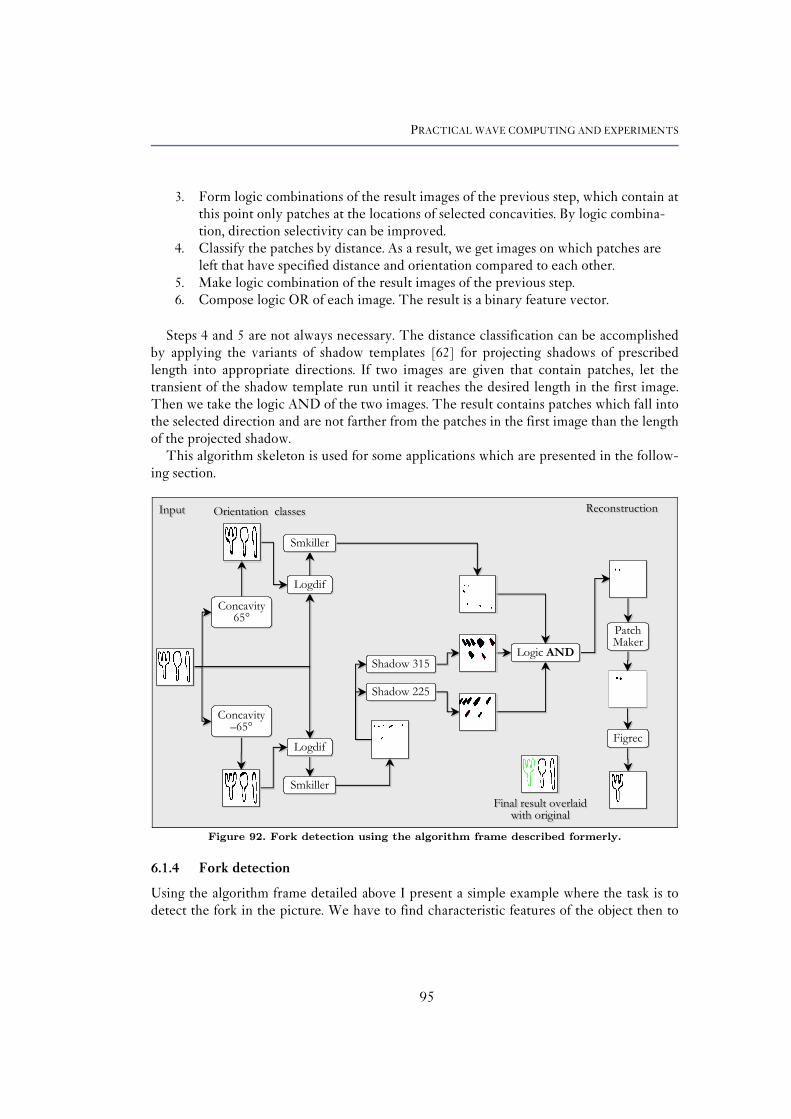
PRACTICAL WAVE COMPUTING AND EXPERIMENTS
3. Form logic combinations of the result images of the previous step, which contain at this point only patches at the locations of selected concavities. By logic combina-tion, direction selectivity can be improved.
4. Classify the patches by distance. As a result, we get images on which patches are left that have specified distance and orientation compared to each other.
5. Make logic combination of the result images of the previous step. 6. Compose logic OR of each image. The result is a binary feature vector.
Steps 4 and 5 are not always necessary. The distance classification can be accomplished
by applying the variants of shadow templates [62] for projecting shadows of prescribed length into appropriate directions. If two images are given that contain patches, let the transient of the shadow template run until it reaches the desired length in the first image. Then we take the logic AND of the two images. The result contains patches which fall into the selected direction and are not farther from the patches in the first image than the length of the projected shadow.
This algorithm skeleton is used for some applications which are presented in the follow-ing section.
InputInput Orientation classesOrientation classes ReconstructionReconstruction
LogdifLogdif
SmkillerSmkillerFinal result overlaid
with originalFinal result overlaid
with original
Concavity 65°
Concavity 65°
LogdifLogdif
SmkillerSmkiller
Shadow 315Shadow 315
Shadow 225Shadow 225
Concavity –65°
Concavity –65°
Logic ANDLogic AND
FigrecFigrec
PatchMakerPatchMaker
Figure 92. Fork detection using the algorithm frame described formerly.
6.1.4 Fork detection
Using the algorithm frame detailed above I present a simple example where the task is to detect the fork in the picture. We have to find characteristic features of the object then to
95

PRACTICAL WAVE COMPUTING AND EXPERIMENTS
extract them. Such features are concavities or endings and their relative position. Some post- and intermediate processing is needed such as small object removing.
The solution starts with applying two direction–selective concavity filters (Step 1). Thus we can fill in the tip and the bifurcations of the fork (see Fig. 92). Next taking the difference of the result and the original we get the locations of the tip and the bifurcation points (step 2).
Following templates were used:
Concavity 65: 2,
000
020
000
,
101
021
100
=⎥⎥⎥
⎦
⎤
⎢⎢⎢
⎣
⎡=
⎥⎥⎥
⎦
⎤
⎢⎢⎢
⎣
⎡= zBA
Concavity –65: 2,
000
020
000
,
100
021
101
=⎥⎥⎥
⎦
⎤
⎢⎢⎢
⎣
⎡=
⎥⎥⎥
⎦
⎤
⎢⎢⎢
⎣
⎡= zBA
Shadow 315: 5.2,
000
04.10
000
,
100
021
011
=⎥⎥⎥
⎦
⎤
⎢⎢⎢
⎣
⎡=
⎥⎥⎥
⎦
⎤
⎢⎢⎢
⎣
⎡
−= zBA
Shadow 225: 5.2,
000
04.10
000
,
001
120
110
=⎥⎥⎥
⎦
⎤
⎢⎢⎢
⎣
⎡=
⎥⎥⎥
⎦
⎤
⎢⎢⎢
⎣
⎡
−= zBA
The Figrec template reconstructs the image starting from one point. The Smkiller tem-plate removes the small, few pixels wide objects. The Figrec, Smkiller and the Patchmaker templates are available in the CNN software library [62]. The Shadow* templates result in directed shadows originating from concave locations.
6.1.5 Hand orientation detection
This algorithm shares the basic principle described in 6.1.3. Supposing a suitably preproc-essed image the algorithm starts with a thresholding. Next the difference of the original and the intermediate results are taken and artifacts are removed. Finally, the nonempty image out of the three intermediate results denotes the detected orientation class.
96

PRACTICAL WAVE COMPUTING AND EXPERIMENTS
InputInput Orientation classesOrientation classes DecisionDecision
ANDAND
ANDAND
ANDAND
UPUP LEFTLEFT DOWNDOWN INVALIDINVALID
LogdifLogdif
SmkillerSmkiller
LogdifLogdif
SmkillerSmkiller
LogdifLogdif
SmkillerSmkiller
Global OR
Global OR
Global OR
Global OR
Global OR
Global OR
=1?=1?=1?=1?
=1?=1?Every pixels
are WHITE?
Every pixels
are WHITE?
Concavity 26°
Concavity 26°
Concavity 63°
Concavity 63°
Concavity 206°
Concavity 206°
Concavity 333°
Concavity 333°
Figure 93. Hand orientation detection by the 64x64 CNNUM chip. The dotted input line of Logdif symbolises the signal source from the black and white input images. The text boxes contain the names of the applied templates and logic operations.
Concavity153°
Concavity153°
Concavity26°
Concavity26°
Concavity333°
Concavity333°
LogdifLogdif
LogdifLogdif
LogdifLogdif
PatchmakerPatchmaker
PatchmakerPatchmaker
PatchmakerPatchmaker
ANDAND
ANDAND
SubtractSubtract Bipolarwave
Bipolarwave
Figure 94. Texton segmentation. The text boxes contain the names of the applied templates and logic operations. The final image contains the regions.
97

PRACTICAL WAVE COMPUTING AND EXPERIMENTS
6.1.6 Texton segmentation
This algorithm is also built according to the steps listed in 6.1.3. However, as a final step segmentation block is added. The segementation applies bipolar waves described in 6.1.2. The result of computation is the steady state of the propagation.
6.2 Mobile navigation unit
The templates and subroutines described previously constitute a basic image processing tool-set. In the following I introduce a mobile surveillance robot (see Fig. 95) of which con-trol algorithm integrates the aforementioned tool-set.
The aim was to design and produce a mobile platform-based system that is able to iden-tify objects or events by simple features (shape, texture, motion, etc.) and to approach or navigate to them. Moreover, it is able to gather information and transmit information about them to the base station. The mobile unit communicates with the base station through a wireless channel. The base station monitors the mobile unit of which control can be taken over at any time.
The robotic system is equipped with several sensors, operates on battery and controlled by the Bi-i system introduced in chapter 3 on page 18. The robot itself is an off-the-shelf mobile platform fabricated by K-Team from Switzerland.
IR proximity sensors Bi–i
Sonar
Wireless internet 802.11b TCP/IP
Air flow sensor
Gas sensor
Figure 95. Mobile unit overview.
6.2.1 Hardware infrastructure
The hardware of the system is the result of collaboration of several partners of the project. The Bi-i system was designed and produced by the Analogic Computers Ltd [108]. The airflow and gas sensors were produced by MTA-KFKI-MFA research institute (see Fig.
98

PRACTICAL WAVE COMPUTING AND EXPERIMENTS
95). The high-level algorithm frame for controlling the mobile unit was designed at MTA-SZTAKI, in which the author took part.
PC
Sensoryplatform
Gas Flow
Bi-i
Visual 1
Visual 2
Koala
US
IR
Wireless bridge
Wireless bridge
Base station
Mobile unit
Figure 96. Block diagram of the mobile sytem.
The block diagram of the system is shown in Fig. 96. Main components are the base sta-tion that consists of a PC with a wireless bridge and the mobile unit. The mobile unit is built up of a mobile platform (Koala), the Bi-i system and the sensory platform. The Koala is a processor controlled mobile platform equipped with IR proximity sensors and sonar (US) that controls the low-level navigation of the car. The Sensory platform hosts the gas and airflow sensors.
Figure 97. Real - virtual environment
99

PRACTICAL WAVE COMPUTING AND EXPERIMENTS
Figure 98. Robot in the test world
The mobile unit is tested in a closed test-world (Fig. 97 and 98) in which different ob-jects or places should be recognized/found by the fused infrared, ultrasound, gas and visual sensory information. Future developments include the virtual representation of the model world and the car. We developed an integrated control environment that provides visual, literal and/or numerical feedback from the robot and allows the user to change parameters, strategy and operation modes of the mobile unit and to interact immediately if necessary (see Fig. 99).
Figure 99. Integrated control environment of the mobile unit.
100

PRACTICAL WAVE COMPUTING AND EXPERIMENTS
6.2.2 Software infrastructure The Bi-i system is responsible for the high-level control. It contains three dedicated
processors (CNN-UM, DSP -digital signal processor, Communication processor). The processor of the robot car is responsible for the control of the motors. It computes a low-level obstacle avoidance algorithm that is modulated by the Bi-i system. The car receives direction and speed commands from the Bi-i that computes the so-called hybrid strategy based mobile robot control algorithm. The main emphasis is put on the visual processing that is the most computationally intensive part of the control architecture (Fig. 100).
The computationally intensive parts of the image processing algorithms run on the CNN-UM. This includes the topographic preprocessing of images (feature and motion extraction and the fusion of them). The DSP controls the CNN-UM, gathers measurements both from the sensory platform and from the robot car. The car provides – if necessary – IR, sonar measurements and homeostatic sensory information. The DSP computes some part of motion analysis and performs post processing necessary for the categorization of infor-mation. The other modules that run on DSP update the world model – a global memory of the space discovered –, determine the goal to be reached (planner module) and perform the integration of the different sensory modalities so as to provide a suitable input to the navi-gation module, that selects the appropriate behaviour (movement) to reach the goal.
In the following I introduce some of the modules that make use of CNN technology.
Pattern recognition
Pattern recognition
World modelWorld model
Navigationmodule
Navigationmodule
Motion analysisMotion analysis
Motion field estimation
Motion field estimation
Visual sensorVisual sensor
SonarSonar
Inner state sensors
Inner state sensors
IR proximity sensors
IR proximity sensors
CNN-UMCNN-UM
RobotRobot
MotorMotor
Bi-I
Visual collision avoidance unitVisual collision avoidance unit
Inner collision avoidance unitInner collision avoidance unit
Planner modulePlanner moduleSensorsSensorsLocalisationLocalisation StrategyStrategy
EffectorEffector
BehaviorsBehaviors
Virtual sensorsVirtual sensors
Figure 100. Mobile unit control architecture.
101

PRACTICAL WAVE COMPUTING AND EXPERIMENTS
6.2.3 Optic flow estimation
Optic flow calculation is a rather computationally intensive step of image processing. Still, its use cannot be omitted because it is one of the key steps of spatio–temporal motion proc-essing. Algorithms found in literature [127] usually include some kind of computationally intensive method e.g. block matching techniques, iterative minimization methods or matrix inversion. However, using simple parallel near–sensory image processing techniques a very fast approximate motion field can be extracted. The result of this method can be used as a first guess for more sophisticated methods or, if the precision is enough, it can be the start-ing point for segmentation and recognition tasks.
Let us consider a moving object. The key element of the algorithm is a fading memory that serves as storage for motion history. The movements of selected features are stored in it such a way that the feature map is iteratively added to the memory. Adding is followed by a thresholding to keep the values bounded. The detected feature is represented in the map with black pixels (maximum intensity level). Meanwhile, the whole memory content is leaking i.e. the intensity of each pixel is gradually decreasing. As an object moves it as added to the memory in a little shifted position depending on its speed. Due to the fading property of the memory a motion history is produced resembling a comet that draws a tail. The head is the actual position of the object feature having maximum intensity; the tail preserves the previous positions with decreasing intensity. The direction of the gradient on this tail gives the direction of the motion and its magnitude is proportional to the inverse of the magnitude of the speed of the object. As a result, a vector field of the moving features (objects) is produced. It is supposed that the feature map is not “too dense”. This supposi-tion is necessary to have enough space for the motion history.
Motion field estimation algorithmMotion field estimation algorithm
InputInput
Feature extractionFeature
extraction
Fading memoryFading
memory++
GradientGradient
Vector fieldVector field
binarybinarybinary
grayscalegrayscalegrayscale
grayscalegrayscalegrayscale
grayscalegrayscalegrayscale
Figure 101. The block diagram of the motion field estimation algo-rithm.
102

PRACTICAL WAVE COMPUTING AND EXPERIMENTS
The faster the object the longer the tail is. The slower the object the higher the gradient is on the tail.
Using several feature maps and fading memories effective motion analyzer algorithms can be built due to the inherent parallel nature of the method proposed.
Due to this it is a completely focal–plane array feasible solution. Electronically the im-age memory can be represented with (fading) capacitors that are charged to maximum value when the corresponding pixel is black. The feature map can be e.g. the time deriva-tive of the input, of which computaion is easy by a hardware. Additional morphological operations such as dilation, or erosion is applied to smooth the feature map.
Figure 102. The original snapshots
Figure 103. The feature map. The image feature is the thresholded temporal derivative of the image flow.
Figure 104. Fading memory: head (white patches) and tail (gray parts) of the motion his-tory map.
103

PRACTICAL WAVE COMPUTING AND EXPERIMENTS
Figure 105. Gradient map. Upper film shows the gradient along x direction, the lower one shows along y direction. White color means positive gradient component, black denotes negative.
Figure 106. Final output. The vector field is overlaid onto the original image flow.
6.2.4 Visual collision avoidance
The algorithm is based on the fact that the obstacle parameters such as area of the object, size of the object, edge quantity, edge speed, etc. change faster as the observer gets more and more closer to the object provided that the observer has constant speed. If the speed of change reaches a prescribed limit we declare a threat of collision and send a signal to the navigation unit.
Figure 107 shows the block diagram of the algorithm. The input frames are grayscale images. Let us consider the last four frames of the image flow. Difference is computed be-tween Framet and Framet-1, Framet-1 and Framet-2, Framet-2 and Framet-3. Then the abso-lute value of the frames are taken. Thus we get three images that are mostly zero and con-tain only black pixels where change occurred. On the first two frames a propagating tem-plate is computed the result of which can predict the possible change of the image.
104

PRACTICAL WAVE COMPUTING AND EXPERIMENTS
Frame tFrame t Frame t-1Frame t-1 Frame t-2
Frame t-2 Frame t-3Frame t-3
I -1I -1 I -2
I -2
I I
Difference image
Difference image ThresholdingThresholding
Collision avoidance algorithm
DangerDanger
Free trackFree track
DifferenceDifference DifferenceDifference DifferenceDifference
Lateral propagation
Lateral propagation
Lateral propagation
Lateral propagation
SuperpositionSuperposition
DifferenceDifference
SummationSummation
Absolute valueAbsolute value Absolute valueAbsolute value Absolute valueAbsolute value
Figure 107. Visual TTC (time to collision) based analogic algorithm.
These two images are added topographically to filter the noise and fluctuations of the frames. The difference between predicted and the last absolute difference image gives a good measure of the speed of change of the edges. The sum of the pixels in the Difference image gives a number. Based on this number we can set a threshold above which the system declares danger in which case the car should immediately stop.
Feature extraction
Visual sensorVisual sensor
Feature extractionFeature extraction
ClassificationClassification
ConcavityConcavity CornersCornersLocal curvature
Local curvature
Tipical shapesTipical shapes
Horizontal positionHorizontal position
Figure 108. Pattern recognition module.
105

PRACTICAL WAVE COMPUTING AND EXPERIMENTS
6.2.5 Feature detection
This algorithm makes use of the methods described in section 5.3.1 and 6.1. The consecu-tive image frames are filtered and thresolded. Then an image is produced for each local feature (curvature, concavity, corners, etc.) that is extracted and bound to the shape they belong to (Fig. 108).
The horizontal position of the detected shape gives the direction information to the navigation module. This information is also integrated to the world model.
6.3 Complex spatio–temporal wave experiments with CNN
The Complex Cell CNN programmable array computer [123,124] is an extension of the CNN Universal Machine [46–49]. The cells are organized into a 32×32 square grid. Each cell has second order dynamics and local interconnections to its neighbors. This structure is especially suitable for computing a certain set of ordinal differential equations. Simple PDEs can be transformed so that they can be easily programmed on the array computer. With the programmable Complex Cell CNN Universal Machine scientists are provided with a unique opportunity to study active-wave propagation and other reaction-diffusion differential equation based phenomena in a programmable manner. Exploiting the inherent programmability of the CNN architecture, complex wave-computing analogic algorithms can be designed.
In the following I describe the mathematical model of the core of the complex cell chip. Section 6.3.3 contains the real-time chip measurements. We should emphasize that no simulation results are presented here. This chip was designed also for computing biologi-cally inspired retina modelling.
The architecture of the chip follows the design of the first order CNN-UM chip [98], but its first order cell core is replaced by a second order one [123]. With this change we are able to reproduce basic autowave phenomena. Fig. 109 shows the functional architecture of the second order, two-layer CNN.
input
layer 1
layer 2
a12 a21y2 A1x1
A2x2 x2x1
τ1
τ2
z1
b2u2
z2
b1u1
τ1 ≥ τ2output Figure 109. Functional diagram of the CACE1k chip
6.3.1 Mathematical model
The evolution law of the complex cell CNN is the following differential equation system:
106

PRACTICAL WAVE COMPUTING AND EXPERIMENTS
( )
( )
10,10,1,1
)()()()(
)()()()(
,22,121,2,2,2,2
2
,11,212,1,1,1,1
1
1
1
≤≤≤≤≤≤≤≤
++++−=
++++−=
∑
∑
∈
∈
ijij
ijijijNkl
klklijij
ijijijNkl
klklijij
xuMjMi
zubtxatxAtxgdt
tdx
zubtxatxAtxgdt
tdx
τ
τ
(6.3)
Where M and N denote the vertical and horizontal dimensions of the array respectively.
( )
( )⎪⎩
⎪⎨
⎧
−<−+≤>+−
=∞→
111
1
111
lim)(
,,
,,
,,
,
ijnijn
ijnijn
ijnijn
mijn
xifxm
xifx
xifxm
xg (6.4)
Function g(.) regulates the state so that the state stays within the +1..-1 interval. Vari-ables u1 and u2 are the independent inputs, b1 and b2 are their weight factors; z1,ij and z2,ij are space variant bias maps. Variables x1 and x2 denote the state variables of the layers. Each xij corresponds to one cell; it is one pixel of an M by N image if we consider the system’s out-put as a picture. A1, A2 are the weights of the intra-layer couplings, a1, a2 are the inter-layer weights; τ1 and τ2 are the time constants of the two layers. Equation (6.3) utilizes the so-called full-range model (FSR)[125], where the voltage of the state variable is always the same as the output.
6.3.2 Stored programmability
The CACE1k chip can be programmed using the so-called AMC (ANALOGIC MACHINE CODE) language. This is similar to the assembler language but it contains additional high-level instructions, such as: image loading, frame grabber instructions, etc. and built in image processing functions. In the Appendix is a simple AMC program which computes the snap-shots of the autowave example. The actual computation is performed in line 40. Before this line is the preparation for computation: setting up the parameters. After the computation is done, the results are read out and displayed from the local analog memories of the chip.
The elementary program of the chip is the template. It contains the weight factors of the coupling between the cells and weights for the input and the bias map.
(6.5)
16..1,1:2121
12212
1,12
0,12
1,1
21,0
20,0
21,0
21,1
20,1
21,1
21
1,11
0,11
1,1
11,0
10,0
11,0
11,1
10,1
11,1
1
==
⎥⎥⎥
⎦
⎤
⎢⎢⎢
⎣
⎡
=⎥⎥⎥
⎦
⎤
⎢⎢⎢
⎣
⎡
=
−
−
−−−−
−
−
−−−−
ττττ 21 :
AA
zzbb
aa
aaa
aaa
aaa
aaa
aaa
aaa
The operation of the array computer is completely determined by the 25 template val-ues, the initial states and boundary conditions. In (6.5) A1 and A2 matrices denote the weights of the inter-layer connections of the slower and the faster layers. The strength of the influence of the second layer on the first is controlled by a21; a12 stands for the reverse case. Symbols b1, b2, z1 and z2 are the weights of the independent inputs and the space vari-ant bias maps. The ratio of the time constants of the two CNN layers are controlled by τ1;τ2 is fixed. An analogic algorithm is made up of combinations of template executions,
107
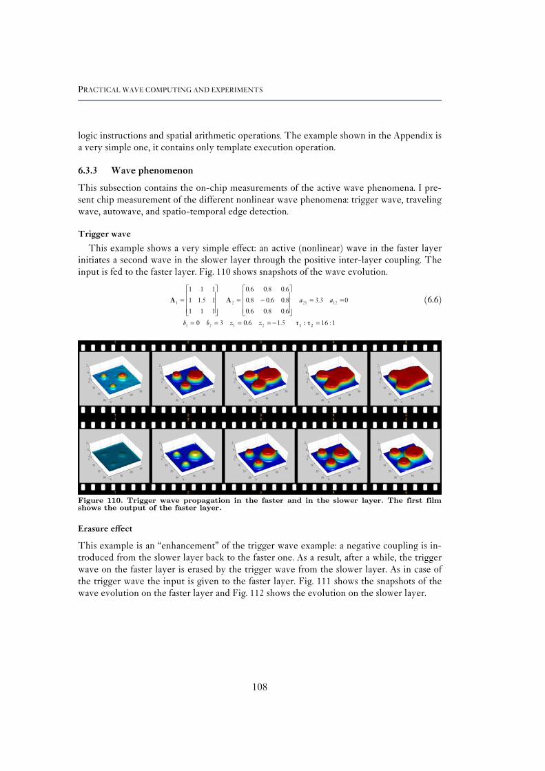
PRACTICAL WAVE COMPUTING AND EXPERIMENTS
logic instructions and spatial arithmetic operations. The example shown in the Appendix is a very simple one, it contains only template execution operation.
6.3.3 Wave phenomenon
This subsection contains the on-chip measurements of the active wave phenomena. I pre-sent chip measurement of the different nonlinear wave phenomena: trigger wave, traveling wave, autowave, and spatio-temporal edge detection.
Trigger wave
This example shows a very simple effect: an active (nonlinear) wave in the faster layer initiates a second wave in the slower layer through the positive inter-layer coupling. The input is fed to the faster layer. Fig. 110 shows snapshots of the wave evolution.
(6.6)
1:165.16.030
03.3
6.08.06.0
8.06.08.0
6.08.06.0
111
15.11
111
2121
122121
=−====
==⎥⎥⎥
⎦
⎤
⎢⎢⎢
⎣
⎡−=
⎥⎥⎥
⎦
⎤
⎢⎢⎢
⎣
⎡=
21 :
AA
ττzzbb
aa
Figure 110. Trigger wave propagation in the faster and in the slower layer. The first film shows the output of the faster layer.
Erasure effect
This example is an “enhancement” of the trigger wave example: a negative coupling is in-troduced from the slower layer back to the faster one. As a result, after a while, the trigger wave on the faster layer is erased by the trigger wave from the slower layer. As in case of the trigger wave the input is given to the faster layer. Fig. 111 shows the snapshots of the wave evolution on the faster layer and Fig. 112 shows the evolution on the slower layer.
108

PRACTICAL WAVE COMPUTING AND EXPERIMENTS
Figure 111. Retina-like wide-field erasure effect, faster layer.
(6.7)
1:167.26.030
4.53.3
6.08.06.0
8.06.08.0
6.08.06.0
111
15.11
111
2121
122121
=−====
−==⎥⎥⎥
⎦
⎤
⎢⎢⎢
⎣
⎡−=
⎥⎥⎥
⎦
⎤
⎢⎢⎢
⎣
⎡=
21 :
AA
ττzzbb
aa
Figure 112. Retina-like wide-field erasure effect, slower layer.
Traveling wave
The characteristic of this wave is that a single wave front travels across the active medium. The traveling wave is simply formed from the trigger wave template by adding a negative intra-layer coupling from the slower to the faster layer. Observe the annihilation property of this wave type in Fig. 113.
109

PRACTICAL WAVE COMPUTING AND EXPERIMENTS
Figure 113. Traveling wave generation.
(6.8)
1:167.26.050
2.45.4
6.08.06.0
8.06.08.0
6.08.06.0
111
15.11
111
2121
122121
=−====
−==⎥⎥⎥
⎦
⎤
⎢⎢⎢
⎣
⎡−=
⎥⎥⎥
⎦
⎤
⎢⎢⎢
⎣
⎡=
21 :
AA
ττzzbb
aa
Target wave
The target waves possess all of the properties of the traveling waves; the difference is that in this case multiple wave fronts are generated. See Fig. 114.
Figure 114. Target wave propagation CACE1k chip.
110

PRACTICAL WAVE COMPUTING AND EXPERIMENTS
(6.9)
1:139.35.130
4.27.5
6.08.06.0
8.09.08.0
6.08.06.0
6.08.06.0
8.06.08.0
6.08.06.0
2121
122121
=−=−===
−==⎥⎥⎥
⎦
⎤
⎢⎢⎢
⎣
⎡−=
⎥⎥⎥
⎦
⎤
⎢⎢⎢
⎣
⎡−=
21 :
AA
ττzzbb
aa
Spiral wave
This type of wave received its name from the spiral-like autowave structure. This phe-nomenon was observed e.g. in biology. Examples are described in the Introduction of this dissertation. Fig. 115 shows measurement results on the CACE1k chip. The annihilation of two wave fronts occurs in this case as well.
Figure 115. Spiral wave formation in the CACE1k chip.
(6.10)
1:86.35.49.30
36
6.08.06.0
8.09.08.0
6.08.06.0
6.08.06.0
8.03.08.0
6.08.06.0
2121
122121
=−=−===
−==⎥⎥⎥
⎦
⎤
⎢⎢⎢
⎣
⎡−=
⎥⎥⎥
⎦
⎤
⎢⎢⎢
⎣
⎡−=
21 :
AA
ττzzbb
aa
Figure 116. Edge detection with second order dynamics on the CACE1k chip. Upper row shows the output of the faster layer, lower row shows the output of the slower one.
111

PRACTICAL WAVE COMPUTING AND EXPERIMENTS
Spatio-temporal edge detection
The basic idea of edge detection in the image processing is to somehow extract or enhance the high frequency components of the image. Here this is done with two layers. The slower layer, which gets its input from the faster one, computes the diffusion. The result is sub-tracted from the faster layer. As a result, we get the edge image of the original image. The input was fed to the faster layer. See snapshots of the transient in Fig 116.
(6.11)
1:60930
7.55.4
000
000
000
5.08.05.0
8.06.38.0
5.08.05.0
2121
122121
==−===
−==⎥⎥⎥
⎦
⎤
⎢⎢⎢
⎣
⎡=
⎥⎥⎥
⎦
⎤
⎢⎢⎢
⎣
⎡−=
21 :
AA
ττzzbb
aa
112

113


REFERENCES
References
[1] V. I Krinsky, V. N. Biktashev, and I. R. Efimov, “Autowave Principles for Image Process-ing”, Physica D 49, pp. 247-253, 1991.
[2] J. S. Russel, “Report of the Committee on Waves,” Report of the 7th Meeting of the British Association for the Advancement of Science (John Murray, London, 1838), pp. 417–496.
[3] V. I. Krinsky and A. M. Zhabotinsky, “Autowave Process in Systems with Diffusion”, Ed. M. T. Grekhova, Gorki IPF Acad. Sci USSR, p. 6, 1981
[4] A. N. Zaikin, A. M. Zhabotinsky, “Concentration waves propagation in two-dimensional liquidphase self-oscillating system,” Nature 225, 535-537, 1970
[5] A.C. Scott, “The electrophysics of a nerve fiber”, Rev. mod. Phys. Vol. 47, pp 487–533, 1975
[6] P. C. Newell, “Microbial Interactions, Receptors and Recognition”, Series B, J. L. Reissig, ed., pp. 1–57, Chapman & Hall, 1977
[7] B. Goodwin, “How the leopard changed its spots”, Charles Scribner’s Sons, New York, 1994
[8] A. M. Turing, “The chemical basis of morphogenesis”, Phil. Trans. R. Soc. London, B327, 37–72 (1952).
[9] I. Prigogine, “From being to becoming”, W. H. Freeman and Company, New York, 1980
[10] Ser. Ed: L. O. Chua, Ed: V. Pérez-Villar V. Pérez-Muñuzuri, Pérez García and V. I. Krin-sky, “New Trends in Pattern Formation in Active Nonlinear Media,” World Scientific Se-ries in Nonlinear Science, Series B, Vol. 3, 1995
[11] L. O. Chua, “CNN: A Paradigm for complexity”, World Scientific Pub Co; ISBN: 981023483X, 1998.
[12] S. Wolfram, A New Kind of Science, Wolfram Media, Inc., Champaign IL, 2002.
[13] S. Wolfram, Cellular Automata and Complexity, Westview press, Member of the Perseus Books Group, 1994.
115

REFERENCES
[14] A. Pérez-Muñuzuri, V. Pérez-Muñuzuri, M. Gómez-Gesteira, L.O. Chua, V. Pérez-Villar, “Spatiotemporal structures in discretely-coupled arrays of nonlinear circuits: A review”, Int. J. Bif. Chaos, Vol. 5, No. 1, pp. 17-50, 1995.
[15] Krinsky, V. I. (ed.) “Self Organization. Autowaves and Structures Far from Equilibrium” (Springer, Berlin, Singapore), pp. 9–19. 1984
[16] E. Schrödinger, “What is Life? The Physical Aspect of the Living Cell & Mind and Matter” University Press, Cambridge, 1967
[17] H. Haken, ”Synergetics: From Pattern Formation to Pattern Analysis and Recognition”, International Journal on Bifurcation and Chaos, Vol. 4, No. 5, pp. 1069-1083, 1994.
[18] H. Haken, Synergetics: An Introduction, Springer Verlag, Berlin, 1978.
[19] H. Haken, Synergetic Computers and Cognition, Springer Verlag, Berlin, 1991.
[20] G. Nicolis, I. Prigogine, “Exploring Complexity,” W. H. Freeman, New York, 1989
[21] C. G. Langton, “Computation at the edge of chaos: Phase transitions and emergent compu-tation,” Physica D, Vol. 42, pp. 12–37, 1990
[22] L. O. Chua, “CNN: a Vision of Complexity”, International Journal of Bifurcation and Chaos, Vol. 7, No. 10, pp. 2219-2425, 1997.
[23] R. Dogaru, L. O. Chua, “Edge of Chaos and Local Activity Domain of the Gierer Meinhardt CNN”, International Journal of Bifurcation and Chaos (IJBC), Vol. 8, No. 12, pp. 2321–2340, 1998
[24] R. Dogaru, L. O Chua, “Edge of chaos and local activity domain of FitzHugh–Nagumo Equation,” Int. J. Bifurcation and Chaos, Vol. 8, No. 2, pp. 211–257, 1998
[25] R. Dogaru, L. O Chua, “Edge of chaos and local activity domain of the Brusselator CNN,” Int. J. Bifurcation and Chaos, Vol. 8, No. 6, 1107–1130. 1998
[26] L. O. Chua, “Passivity and Complexity”, IEEE Trans. on Circuits and Systems, Vol. 46, No. 1, 1999.
[27] J. P. Keener, “Propagation and its Failure in Coupled Systems of Discrete Excitable Cells”, SIAM J. Appl. Math., Vol. 47, 556-572, 1987.
[28] H. Meinhardt, The Algorithmic Beauty of Sea Shells (The Virtual Laboratory Series), Springer-Verlag New York, ISBN: 3540440100, 2003
[29] M. Allesie, F. I. M. Bonke, J.G. Schopman, , “Circus movement in rabbit atrial muscle as a mechanism of tachycardia,” Circ. Res. 33, 54-62.
[30] L. O. Chua, S Yoon, R. Dogaru, “A nonlinear dynamics perspective of Wolfram’s New Kind of Science. Part I: Threshold of Complexity”, International Journal of Bifurcation and Chaos, Vol. 12, No. 12, 2655–2766, 2002
[31] L. O. Chua, Ed., “Special Issue on Nonlinear Waves, Patterns and Spatio-Temporal Chaos in Dynamic Arrays,” IEEE Transactions on Circuits and Systems: I, vol. 42, no. 10, Oct. 1995.
[32] J. Weickert, “A review of nonlinear diffusion filtering”, (Invited Paper), Scale-Space Theory in Computer Vision, Lecture Notes in Comp. Science (Springer, Berlin), 1252:3-28, 1997.
116

REFERENCES
[33] B.M.H. Romeny (ed.), “Geometry-driven Diffusion in Computer Vision,” Kluwer Aca-demic Publishers, 1994.
[34] A.P. Witkin, “Scale-space filtering,” Proc. Eighth Int. Joint Conf. on Artificial Intelligence (IJCAI ’83), vol.2, pp.1019-1022, 1983.
[35] P. Perona and J. Malik, “Scale-Space and Edge Detection Using Anisotropic Diffusion”, IEEE Trans. on Pattern Analysis and Machine Intelligence, Vol. 12, pp.629-639, July 1990.
[36] N. Nordström, “Biased Anisotropic Diffusion – A Unified Regularization and Diffusion Approach to Edge Detection”, Image Vision Computers, Vol.8, No 4,pp.318-327,July 1990.
[37] L. Alvarez, P. L. Lions, and J. M. Morel, "Image Selective Smoothing and Edge Detection by Nonlinear Diffusion. II", SIAM Journ. on Num. Analysis, Vol. 29, No. 3, pp. 845-866, 1992.
[38] F. Catté, P.L. Lions, J. M. Morel and T. Coll, “Image Selective Smoothing and Edge Detec-tion by Nonlinear Diffusion”, SIAM Journal on Numerical Analysis, Vol.29, No.1, pp.182-193, 1992.
[39] D. Terzopoulos, A. Witkin and M. Kass, “Constraints on deformable models:Recovering 3D shape and nonrigid motion,” Artificial Intelligence, Vol. 36, Issue 1, pp. 91-123, August 1988,
[40] M. Kass, A. Witkin, and D Terzopolous, “Snakes: active contour models,” Int. Journal of Computer Vision, 1:321–331, 1988.
[41] L. C. Evans, J. Spruck, “Motion of level sets by mean curvature I,” J. Differential Geometry, 33 (1991), pp. 635-681
[42] S. Osher, and J. A. Sethian, “Fronts Propagating with Curvature Dependent Speed: Algo-rithms Based on Hamilton-Jacobi Formulation”, Journal of Computational Physics, Vol. 79, pp. 12-49, 1988.
[43] G. Sapiro, “From Active Contours to Anisotropic Diffusion: Connections between Basic PDE's in Image Processing”, Proceedings 3rd IEEE International Conference on Image Processing (ICIP'96), Lausanne, Suisse, September 1996.
[44] B. B. Kimia & K. Siddiqi, “Geometric Heat Equation and Nonlinear Diffusion of Shapes and Images”, Computer Vision and Image Understanding, 64(3), 305-322, 1996.
[45] J. Weickert, “Applications of Nonlinear Diffusion in Image Processing and Computer Vi-sion,” Acta Math. Univ. Comenianae, LXX(1):33--50, 2001.
[46] L. O. Chua and L. Yang, “Cellular Neural Networks: Theory”, IEEE Trans. on Circuits and Systems, Vol. 35, pp. 1257-1272, Oct. 1988.
[47] L. O. Chua and L. Yang, “Cellular Neural Networks: Applications”, IEEE Trans. on Circuits and Systems, Vol. 35, pp. 1273-1290, Oct. 1988.
[48] L. O. Chua, and T. Roska, “The CNN Paradigm”, IEEE Trans. on Circuits and Systems, Vol. 40, pp.147-156, March 1993.
[49] T. Roska and L. O. Chua, “The CNN Universal Machine: an Analogic Array Computer”, IEEE Trans. on Circuits and Systems, Vol. 40, pp. 163-173, March 1993.
[50] H. Harrer, J.A.Nossek, T. Roska, L.O. Chua, “A Current-mode DTCNN Universal Chip”, Proc. of IEEE Intl. Symposium on Circuits and Systems, pp135-138, 1994.
117

REFERENCES
[51] J.M. Cruz, L.O. Chua, and T. Roska, “A Fast, Complex and Efficient Test Implementation of the CNN Universal Machine”, Proc. of the third IEEE Int. Workshop on Cellular Neural Networks and their Application (CNNA-94), pp. 61-66, Rome Dec. 1994.
[52] R. Dominguez-Castro, Servando Espejo, A. Rodriguez-Vázquez, R. Carmona, P. Földesy, Á. Zarándy, P. Szolgay, T. Szirányi and T. Roska “A 0.8 µm CMOS 2-D programmable mixed-signal focal-plane array-processor with on-chip binary imaging and instructions storage” Vision Chip with Local Logic and Image Memory, IEEE J. of Solid State Circuits 1997
[53] A. Paasio, A. Kananen and V. Porra, "A 176 x 144 processor binary I/O CNN-UM chip de-sign", European Conference on Circuit Theory and Design - ECCTD'99, Design Automa-tion Day proceedings, (ECCTD'99-DAD), Stresa, Italy, 1999
[54] S. Espejo, R. Domínguez-Castro, G. Liñán, and Á. Rodriguez-Vázquez, “A 64x64 CNN universal chip with analog and digital I/O” Proc. 5 th Int. Conf. on Electroonics, Circuits and Systems (ICECS-98), Lisbon, Portugal, pp. 203-206 1998.
[55] G. Liñán, R. Domínguez-Castro, S. Espejo, A. Rodríguez-Vázquez, “ACE16k: A Program-mable Focal Plane Vision Processor with 128 x 128 Resolution”. ECCTD ’01 - European Conference on Circuit Theory and Design, pp.:345-348, August 28-31,2001, Espoo, Finland
[56] V.M. Brea, A. Passio, D.L. Vilariño and D. Cabello, “A DTCNN CMOS Implementation of a Pixel-Level Snake Algorithm,” ECCTD'01 - European Conference on Circuit Theory and Design, Vol. II, pp. 269 - 272. August, 2001, Espoo, Finland.
[57] Á. Zarándy, R. Domínguez-Castro, S. Espejo “Ultra-high frame rate focal plane image sen-sor and processor”, IEEE Sensor Journal, December 2002
[58] R. Carmona, F. Jiménez-Garrido, R. Domínguez-Castro, S. Espejo, T. Roska, Cs. Rekeczky, I. Petrás and A. Rodríguez-Vázquez, "A Bio-Inspired two-Layer Mixed-Signal Flexible Programmable Chip for Early Vision". IEEE Transactions on Neural Networks, vol. 14, issue 5, pp. 1313-1336, ISSN 1045-9227, 2003
[59] I. Petrás, C. Rekeczky, T. Roska, R. Carmona, F. Jimenez-Garrido, and A. Rodriguez-Vazquez, “Exploration of Spatial-Temporal Dynamic Phenomena in a 32×32-Cells Stored Program 2-Layer CNN Universal Machine Chip Prototype”, Journal of Circuits, Systems, and Computers (JCSC) Vol. 12, No. 6, 2003
[60] Á. Zarándy, T. Roska, P. Szolgay, S. Zöld, P. Földesy and I. Petrás, "CNN Chip Prototyp-ing and Development Systems", European Conference on Circuit Theory and Design - ECCTD'99, Stresa, Italy, 1999.
[61] T. Roska, Á. Zarándy, S. Zöld, P. Földesy and P. Szolgay, "The Computational Infrastruc-ture of Analogic CNN Computing - Part I: The CNN-UM Chip Prototyping System", IEEE Trans. on Circuits and Systems I: Vol. 46, No.2, pp. 261-268, 1999.
[62] “CNN Software Library (Templates, subroutines, and Algorithms) Version 8.1”, Edited by T. Roska, L. Kék, L. Nemes, Á. Zarándy, Computer and Automation Institute of the Hun-garian Academy of Sciences, Budapest, 1999
[63] I. Szatmári, P. Földesy, Cs. Rekeczky, Á. Zarándy “Image Processing Library for the Alad-din Visual Computer,” Proceedings of the CNNA-2002 Frankfurt, Germany.
118
REFERENCES
[64] C. Rekeczky and L. O. Chua, “Computing with Front Propagation: Active Contour and Skeleton Models in Continuous-Time CNN,“ Journal of VLSI Signal Processing Special Issue: Spatio-temporal Signal Processing with Analogic CNN Visual Microprocessors, vol. 23, 1999, pp. 373-402.
[65] I. Szatmári, A. Schultz, C. Rekeczky, T. Kozek, T. Roska and L. O. Chua, “Bubble-Debris Classification via Binary Morphology and Autowave Metric on CNN,” IEEE Trans. on Neural Networks, vol. 11, 2000, pp. 1385-1393.
[66] I. Szatmári, C. Rekeczky and T. Roska, “A nonlinear wave metric and its CNN implemen-tation for object classification,” Journal of VLSI Signal Processing Special Issue: Spatiotem-poral Signal Processing with Analogic CNN Visual Microprocessors, vol. 23, 1999, pp. 437-448.
[67] Cs. Rekeczky, T. Roska and A.Ushida, “CNN-based difference-controlled adaptative nonlinear image fiters,” Int. J. Circuit Theory and Applicat.,vol.26,pp.375-423,1998.
[68] Cs. Rekeczky, “CNN architectures for constrained diffusion based locally adaptative image processing,” Int. J. Circuit Theory and Applicat.,vol.30,pp.313-348,2002.
[69] P. Arena, L. Fortuna, M. Branciforte, “Reaction-Diffusion CNN Algorithms to Generate and Control Artificial Locomotion,” IEEE Transaction on Circuits and Systems, I: Fundam. Theory and Applic., Vol. 46 No. 2, pp.259-266, Feb. 1999
[70] D. Bálya, B. Roska, T. Roska, F. S. Werblin: “A CNN framework for modeling parallel processing in a mammalian retina”, Intl. Journal on Circuit Theory and Applications (CTA), Vol. 30, 2002
[71] T. Roska and Á. Rodríguez-Vázquez: “Spatiotemporal Signal Processing with Analogic CNN Visual Microprocessors", Journal of VLSI Signal Processing-Systems for Signal, Im-age, and Video Technology, (JVSP), Vol. 23. No.2/3. Kluwer, ISSN 0922-5773, 1999.
[72] K. R. Crounse and L. O. Chua, “Methods for Image Processing in Cellular Neural Net-works: A Tutorial”, IEEE Trans. on Circuits and Systems, Vol. 42, No. 10, pp. 583-601, October 1995.
[73] K. R. Crounse and L. O. Chua, “A Synergetics Approach to Image Processing in Cellular Neural Networks”, in Proceedings 1996 International Symposium on Circuits and Systems IS-CAS’96, Vol. 3, pp. 134-137, May 1996.
[74] P. Arena, A. Basile, L., Mattia , “CNN Wave Based Computation for Robot Navigation Planning,” Proc. of ISCAS 2004, 2004
[75] Cs. Rekeczky, T. Roska, “Calculating Local and Global PDEs by Analogic Diffusion and Wave Algorithms”, Proc. of ECCTD01, Vol. 2, pp. 17- 20, Espoo, Finland, 2001
[76] F. Corinto, M. Biey, M. Gilli, “Nonlinear PDE Based Cellular Neural Network Models”, Proc. of ECCTD03, Vol.II, pp. 440- 443, Cracow, Poland, 2003
[77] V. Perez-Muñuzuri, V. Perez-Villar, and L. O. Chua, “Autowaves for image processing on a two-dimensional CNN array of excitable nonlinear circuits: Flat and wrinkled labyrinth,” IEEE Trans. Circuits Syst. I, vol. 40, pp. 174–181, Mar. 1993.
119

REFERENCES
[78] A, Perez-Muñuzuri, V. Perez-Muñuzuri, V. Perez-Villar, and L. O. Chua, “Spiral waves on a 2-D array of nonlinear circuits,” IEEE Trans. Circuits Syst. I, vol. 40, pp. 872–877, Nov. 1993.
[79] V. Pérez-Muñuzuri, A.P. Muñuzuri, M. Gómez-Gesteira, V. Pérez-Villar, L. Pivka and L.O. Chua, “Nonlinear Waves, Patterns and Spatio-Temporal Chaos in Cellular Neural Net-works,” Philosophical Transactions of the Royal Society of London, Series A. 353, pp. 101-113, 1995
[80] L. O. Chua, M. Hasler, G. S. Moschytz and J. Neirynck, “Autonomous Cellular Neural Networks: A Unified Paradigm for Pattern Formation and Active Wave Propagation,” IEEE Trans. on Circuits and Systems I: Fundamental Theory and Applications, vol. 42, pp. 559-577, 1995.
[81] T. Roska, L. O. Chua, D. Wolf, T. Kozek, R. Tetzlaff, and F. Puffer, “Simulating Nonlinear Waves and Partial Differential Equations via CNN - Part I: Basic Techniques”, IEEE Trans. on Circuits and Systems, Vol. 42, No. 10, pp. 807-815, October 1995.
[82] T. Kozek, L. O. Chua, T. Roska, D. Wolf, R. Tetzlaff, F. Puffer, K, Lotz, “Simulating Nonlinear Waves and Partial Differential Equations via CNN - Part II: Typical Examples”, IEEE Trans. on Circuits and Systems, Vol. 42, No. 10, pp. 816-821, October 1995.
[83] Cs. Rekeczky, I. Szatmári, and P. Földesy, “Computing on Silicon with Trigger-waves: Ex-periments on CNN-UM Chips”, IEEE International Symposium on Circuits and Systems ISCAS 2001, Sydney, 2001
[84] Cs. Rekeczky, I. Petrás, I. Szatmári and P. Földesy “Active Wave Computing on Silicon: Chip Experiments”, IEEE European Conference on Circuit Theory and Design - ECCTD 2003, Krakow, pp. II-430-433, Sept., 2003
[85] I. Petrás, T. Roska, "Application of Direction Constrained and Bipolar Waves for Pattern Recognition" Int. Workshop on Cellular Neural Networks and Their Applications (CNNA2000), Proc., pp. 3-8, Catania, Italy, 2000
[86] M. Gage & R. S. Hamilton “The heat equation shrinking convex plane curves,” J. Diff. Geom., vol. 23, pp. 69-96, 1986.
[87] M. A. Grayson “The heat equation shrinks embedded plane curves to round points,” J. Diff. Geom., vol. 29, pp. 285-314, 1987.
[88] F. Mokhtarian, A. Mackworth, “A Theory of Multiscale, Curvature-Based Shape Representation for Planar Curves,” IEEE PAMI, Vol. 14, No. 8, pp. 789-805,1992
[89] J. J. Koenderink and A. J. van Doorn, “Dynamic shape. Biolological Cybernetics,” Vol. 53, pp. 383-396, 1986.
[90] B. Kimia, A. Tannenbaum, and S. Zucker, “Shape, shocks, and deformations I: The compo-nents of two-dimensional shape and the reaction-diffusion space,” International Journal of Computer Vision, Vol. 15, pp. 189-224, 1995.
[91] P. Thiran, K. R. Crounse, L. O. Chua, and M. Hasler, “Pattern formation properties of autonomous cellular neural networks”, IEEE Trans. Circuits Syst. I, vol. 42, pp. 757–774, Oct. 1995.
120

REFERENCES
[92] C. Serpico, G. Setti, P. Thiran, S. Callegari, “Comparing Dynamic Behaviour in 1-D CNNs and Reaction-Diffusion-Convection PDEs: a Review”, ECCTD01, ESPOO Finland, 2001, pp. II-29-32
[93] M. Biey, P. Checco, and M. Gilli, “Bifurcation and chaos in CNNs”, Journal of Circuits Sys-tems and Computers, vol. 12, no. 4, pp. 417-433, August 2003.
[94] F. A. Savaci and J. Vandewalle, “On the Stability Analysis of Cellular Neural Networks,” IEEE Trans. on Circuits and Systems I: Fundamental Theory and Applications, vol. 40, 1993
[95] D. Ziou, S. Tabbone, “Edge Detection Techniques - An Overview,” International Journal of Pattern Recognition and Image Analysis, Vol. 8, No. 4, pp. 537-559, 1998.
[96] B.M.H. Romeny (ed.), Geometry-driven Diffusion in Computer Vision, Kluwer Academic Publishers, pp. 49, 1994.
[97] A. Rodriguez-Vázquez, S. Espejo, R. Dominguez-Castro, J.L. Huertas, and E.Sánchez-Sinencio, “Current-Mode Techniques for the Implementation of Continuous- and Dis-crete-Time Cellular Neural Networks”, IEEE Trans. Circuits and Systems II: Analog and Digital Signal Processing, Vol.40. No.3. pp. 132-146, 1993
[98] G. Liñán, S. Espejo, R. Dominguez-Castro and A. Rodríguez-Vázquez, “ACE4k: an Analog I/O 64x64 Visual Microprocessor Chip with 7-bit Analog Accuracy”, International Journal of Circuit Theory and Applications, Vol.30, pp.89-116, 2002
[99] L. Chua and T. Roska, “Cellular neural networks and visual computing - Foundations and applications”, Cambridge University Press, ISBN: 0521652472, 2001.
[100] F. Zou and J. A. Nossek, “Stability of cellular neural networks with opposite-sign tem-plates,” IEEE Trans. Circuits Syst. I, vol. 38, pp. 675–677, 1991.
[101] P. Thiran, G. Setti, and M. Hasler, “An Approach to Information Propagation in 1-D Cellu-lar Neural Networks - Part I: Local Diffusion” IEEE Trans. on Circuits and Systems, Vol. 45, No. 8, pp. 777-789, 1998.
[102] G. Setti, P. Thiran, and M. Hasler, “An Approach to Information Propagation in 1-D Cellu-lar Neural Networks - Part II: Global Propagation” IEEE Trans. on Circuits and Systems, Vol. 45, No. 8, pp. 790-811, 1998.
[103] F. Zou and J. A. Nossek, “Bifurcation and chaos in cellular neural networks,” IEEE Trans. Circuits Syst. I, vol. 40, pp. 166–173, Mar. 1993.
[104] M. Biey, M. Gilli, P. Checco, “Complex dynamic phenomena in space-invariant cellular neural networks”, IEEE Transactions on Circuits and Systems I: Fundamental Theory and Applica-tions, Volume: 49 Issue: 3 , March 2002 pp. 340 -345.
[105] G. Manganaro, P. Arena, L. Fortuna “Cellular Neural Networks: Chaos, Complexity and VLSI Processing”, Springer Verlag, New York; ISBN: 3540652027, 1999
[106] L. O . Chua and T. Roska, “Stability of a Class of Nonreciprocal Cellular Neural Net-works”, IEEE Trans. on Circuits and Systems, Vol. 37, No. 12, pp. 1520-1527, 1990.
[107] T. Roska and A. Rodríguez-Vázquez (editor), “Towards the Visual Microprocessor: VLSI Design and the Use of Cellular Network Universal Machines”, John Wiley & Sons; ISBN: 0471956066, 2000.
121

REFERENCES
[108] The ALADDIN System, http://www.analogic-computers.com/
[109] C. W. Wu and L. O. Chua, “A More Rigorous Proof of Complete Stability of Cellular Neu-ral Networks”, IEEE Trans. on Circuits and Systems, Vol. 44, No. 4, pp. 370-371, 1997.
[110] M. Gilli, “Stability of Cellular Neural Networks and Delayed Cellular Neural Networks with Nonpositive Templates and Nonmonotonic Output Functions,” IEEE Trans. on Circuits and Systems I: Fundamental Theory and Applications, pp. 518-528, vol. 41, 1994
[111] G. De Sandre, “Stability of 1-D-CNN's with Dirichlet Boundary Conditions and Global Propagation Dynamics,” IEEE Trans. on Circuits and Systems I: Fundamental Theory and Applica-tions, vol. 47, pp. 785-792, 2000.
[112] P. P. Civalleri and M. Gilli, “Global dynamic behaviour of a three cell connected compo-nent detector CNN," International Journal of Circuit Theory and Applications, vol. 23, no. 2, pp. 117-135, March 1995.
[113] N. Takahashi and T. Nishi, “On the Global Stability of Two-Cell Cellular Neural Net-works with Opposite-Sign Connections,” Proceedings of the 15th European Conference on Circuit Theory and Design, vol.3, pp.93-96, August 2001.
[114] P. P. Civalleri and M. Gilli, “A Spectral Approach to the Study of Propagation Phenomena in CNNs”, Int. J. Circuit Theory and Applications, vol. 24, 1996, pp. 37-48.
[115] M. Gilli,”Analysis of periodic oscillations in finite-dimensional CNNs through a spatio-temporal harmonic balance technique,” Int. J. Circuit Theory and Applicat., vol. 25, pp. 279-288, July-August 1997.
[116] Zou, F. & Nossek, J. A. “A chaotic attractor with cellular neural networks” IEEE Trans. Cir-cuits Syst. I, vol. 38, 811-812, 1991.
[117] M. Gilli,”Strange attractors in delayed cellular neural networks,” IEEE, Trans. Circuits and Syst.-I, vol. 40, 1993, pp. 849-853.
[118] I. Petrás, Tamás Roska, Leon O. Chua “New Spatial-Temporal Patterns and The First Programmable On-Chip Bifurcation Test-Bed” IEEE Trans. on Circuits and Systems I, (TCAS I.), pp. 619-633, May 2003
[119] P. Thiran, ”Influence of Boundary Conditions on the Behaviour of Cellular Neural Net-works,” IEEE Trans. on Circuits and Systems I: Fundamental Theory and Applications, vol. 40, 1993
[120] I. Petrás, P. Checco, M. Gilli, and T. Roska, “On the Effect of Boundary Condition on CNN Dynamics: Stability and Instability; Bifurcation Processes and Chaotic Phenomena”, Proc. of ISCAS 2003, pp. III 590-593, 2003
[121] J.P. Eckmann and D. Ruelle, “Ergodic Theory of Chaos and Strange Attractors”, Review of Modern Physics, vol. 57, pp. 617-659, 1985.
[122] N.Takahashi and L.O.Chua, “On the Complete Stability of Nonsymmetric Cellular Neural Networks”, IEEE Trans. Circuits and Systems-I, vol.45, no.7, pp.754-758, July 1998.
[123] Cs. Rekeczky, T. Serrano-Gotarredona, T. Roska and A. Rodríguez-Vázquez, “A Stored Program 2nd Order/3-Layer Complex Cell CNN-UM”, Proc. Sixth IEEE Intern. Workshop on Cellular Neural Networks and their Applications, Catania, Italy, May 2000, pp.219-224.
122

REFERENCES
[124] R. Carmona, F. Jiménez-Garrido, R. Domínguez-Castro, S. Espejo and A. Rodríguez-Vázquez, “Bio-inpired Analog VLSI Design Realizes Programmable Complex Spatio-Temporal Dynamics on a Single Chip”. Proc. Design, Automation and Test in Europe Conference (DATE'02), pp. 362-366. Paris, France, March 2002. Published by the IEEE Computer Soci-ety, Los Alamitos, CA, ISBN 0-7695-1471-5.
[125] S. Espejo, R. Carmona, R. Domínguez-Castro and A.Rodríguez-Vázquez, “A VLSI Oriented Continuous-Time CNN Model”. Intern. J. Circuit Theory and Applications, John Wiley&Sons, 24, No.3, May-June 1996, pp.341-356.
[126] Fujita, K. Tanaka, M. Ito and K. Cheng, “Columns for visual features of objects in monkey inferotemporal cortex”, Nature 360, pp. 343-346, 1992.
[127] J.L. Barron, D.J. Fleet, S.S. Beauchemin, ”Performance Of Optical Flow Techniques”, Int J of Comp Vis, vol. 12, no. 1, pp. 43-77, 1994.
[128] Zarándy, A., Domínguez- Castro, R., Espejo, S.: "Ultra-high Frame Rate Focal Plane Image Sensor and Processor". IEEE- Sensors Journal, IEEE. Vol. 2 . Num. 6 - Dec. 2002. pp. 559-565
[129] Á. Zarándy, Cs. Rekeczky, I. Szatmári, “Vision Systems Based on the 128x128 Focal Plane Cellular Visual Microprocessor Chips”, Proc. of ISCAS 2003, pp. III 518-521, 2003
[130] V. Gál, J. Hámori, T. Roska, D. Bálya, Zs. Borostyánkői, M. Brendel, K. Lotz, L. Négyessy, L. Orzó, I. Petrás, Cs. Rekeczky, J. Takács, P. Venetiáner, Z. Vidnyánszky and Á. Zarándy “Receptive Field Atlas and Related CNN Models”, International Journal of Bifurcation and Chaos (IJBC), Vol. 14(2),pp. 551–584, February 2004
[131] D. Bálya, I. Petrás, T. Roska, R. Carmona, A. Rodríguez-Vázquez “Implementing the Multi-Layer CNN Retina Model on the Complex-Cell Stored Program 2-Layer CNN Universal Machine Chip Prototype”, Int. Journal of Bifurcation and Chaos, (IJBC), Vol. 14(2), pp. 551–584, 2004,
[132] I. Petrás, T. Roska, "New spatial-temporal patterns and the first programmable on-chip bi-furcation test-bed", Proceedings of 7th IEEE International Workshop on Cellular Neural Networks and their Applications, Frankfurt, Germany, 2002
[133] P. Szolgay, K. László, L. Kék, T. Kozek, L. Nemes, I. Petrás, Cs. Rekeczky, I. Szatmári, Á. Zarándy, S. Zöld and T. Roska, "The CADETWin Application Software Design System - A Tutorial", European Conference on Circuit Theory and Design - ECCTD'99, Design Automation Day proceedings, (ECCTD'99-DAD), Stresa, Italy, 1999
[134] P. Szolgay, Á. Zarándy, S. Zöld, T. Roska, P. Földesy, L. Kék, T. Kozek, K. László, I. Petrás, Cs. Rekeczky, I. Szatmári and D. Bálya, "The Computational Infrastructure for Cellular Visual Microprocessors", Proceedings of Seventh Int. Conf. on Microelectronics for Neural, Fuzzy, and Bio-Inspired Systems, (MicroNeuro'99), pp. 54-60, Granada, IEEE Computer Society, 0-7695-0043- 9, 1999
[135] M. Gilli, T. Roska, L. O. Chua and P. P. Civalleri, “CNN Dynamics Represents a Broader Class than PDEs”, International Journal of Bifurcation and Chaos, Vol.12, pp.2051-2068, 2002
123

REFERENCES
[136] F. Cortino, M. Gilli, “Comparision between the dynamic behaviour of Chua-Yang and Full-Range cellular neural networks”, (CAS,in press).
[137] M. Gilli, F. Corinto, M. Biey, P. P. Civalleri, “On the dynamic behaviour of cellular neural networks,” Proc. of IJCNN 2002, pp. 1936–1941, 2002
[138] B. E. Shi, "Order Statistic Filtering with Cellular Neural Networks,"Proceedings of IEEE Int. Workshop on Cellular Neural Networks and Their Applications, vol. , 1994, pp. 441-444.
[139] P. Arena, S. Baglio, L.Fortuna, G. Manganaro, “Dynamics of state controlled CNNs”, Proc of ISCAS’96, Vol. 3, pp. 56–59,1996
[140] I.Prigogine, “Nonlinear Science and the Laws of Nature,” International Journal of Bifurca-tion and Chaos, Vol. 7, No. 9, 1917-1926, 1997
[141] H. Haken, “Vision of Synergetics,” International Journal of Bifurcation and Chaos, Vol. 7, No. 9, 1927-1951, 1997
[142] H. Meinhardt, “Biological Pattern Formation as A Complex Dynamic Phenomenon,” Inter-national Journal of Bifurcation and Chaos, Vol. 7, No. 1, 1-26, 1997
[143] A. V. Holden, M. J. Poole and J. V. Tucker, “An algorithmic model of the mammalian heart: propagation, vulnerability, re-entry and fibrillation,” International Journal of Bifurcation and Chaos, Vol. 6, No. 9–10, 1623-1636, 1996.
[144] V. I. Sbitnev, A. O. Dudkin, “Checkerboard Spiral Waves in a 2d Coupled Map Lattice. Scaling Evidence”, International Journal of Bifurcation and Chaos, Vol. 9, No. 5, , pp. 919–928, 1999
[145] S. Paul, K. Hüper, J. A. Nossek and L. O. Chua, "Mapping Nonlinear Lattice Equations onto Cellular Neural Networks,"IEEE Trans. on Circuits and Systems I: Fundamental Theory and Applications, vol. 40, pp. 196-203, 1993
[146] St. Jankowski, C. Mazur, R. Wanczuk, "A CNN model of lattice gas", Proceedings of 11 European Conference on Circuit Theory and Design, (ECCTD'93), pp.699-702, Davos, 1993,
[147] P. C. Newell, “Attraction and adhesion in the slime mold Dyctyostelium,” in Fungal Differ-entiation: A Contemporary Synthesis ed. Smith, J. E., Micology Series 43 (Marcel Dekker, NY), p. 43, 1983
[148] K.Kaneko, Ed., Theory and applications of coupled map lattices, John Wiley & Sons, Chichester, 1993.
[149] K. Kaneko, I. Tsuda, Chaos and Beyond, ISBN 3540672028, Springer Verlag, New York, 2001, pp 57-106.
[150] E.R. Kandel, J.H. Schwartz, “Principles of Neural Science”, second edition, Elsevier, New York, Amsterdam, Oxford, 1985
[151] A. Sanz-Anchelergues, A. P. Munuzuri, “Experimental and Quantitative Modeling Studies of Turing Pattern Formation Under Stochastic Spatial Fluctuations”, International Journal of Bifurcation and Chaos, Vol. 11, No. 11 ,2739–2749, 2001
[152] L. Goras, L. O. Chua and D. M. W. Leenaerts, “Turing patterns in CNNs–Part I, once over lightly”, IEEE Trans. Circuits and Systems–Part I, 42, 602–611 (1995).
124

REFERENCES
[153] L. Goras and L. O. Chua, “Turing patterns in CNNs–part II: equations and behaviours” IEEE Trans. Circuits and Systems –Part I, 42, 612–626 (1995).
[154] L. Goras, L. O. Chua and L. Pivka, “Turing patterns in CNNs-part III: computer simulation results”, IEEE Trans. circuits Systems - Part I, 42, 627-637 (1995).
[155] R. N. Madan, Ed., “Chua’s Circuit: A Paradigm for Chaos,” Singapore, World Scientific, 1993
[156] Szabolcs Tőkés, László Orzó, Ahmed Ayoub and Tamás Roska, “Flexibly Programmable Opto-Electronic Analogic CNN Computer (POAC) Implementation Applying an Efficient, Unconventional Optical Correlator Architecture”, Special Issue on “CNN Technology and Visual Microprocessors", Journal of Circuits, Systems and Computers, vol. 12, no. 6, pp. 739-767, December 2003
[157] S. Tőkés, L.R. Orzó, G. Váró, A. Dér, P. Ormos and T. Roska, "Programmable Analogic Cellular Optical Computer using Bacteriorhodopsine as Analog Rewritable Image Mem-ory", NATO Book: "Bioelectronic Applications of Photochromic Pigments" (Eds.: L. Kesz-thelyi, J. Stuart and A. Der) IOS Press, Amsterdam, Netherlands, pp 54-73. 2000
[158] M. Di Marco, A. Tesi and M. Forti, “Bifurcations and oscillatory behaviour in a class of competitive Cellular Neural Networks,” Int. Journal of Bifurcation and Chaos, Vol. 10, pp. 1267-1293, 2000
[159] M. Di Marco, M. Forti and A. Tesi, “Existence and Characterization of Limit Cycles in Nearly Symmetric Neural Networks”, IEEE Transactions on Circuits and Systems-I: Fun-damental Theory and Applications, Vol.49, No.8, pp.979-992, 2002
[160] M. Di Marco, M. Forti and A. Tesi, “Complex Dynamics in Nearly Symmetric Three-Cell Cellular Neural Networks”, Int. Journal of Bifurcation and Chaos, Vol. 12, No. 6, pp. 1357-1362, 2002
[161] I. Petrás, T. Roska, “CNN as Curve Shortening Flow Computer”, Proceedings of 8th IEEE In-ternational Workshop on Cellular Neural Networks and their Applications, Budapest, Hungary, 2004
[162] J. E. Hopcroft, R. Motwani, J. D. Ullman, “Introduction to Automata Theory, Languages and Computation”, Addison Wesley, 2000.
[163] B. Roska, F.S. Werblin, “Vertical Interactions Across Ten Parallel Stacked Representations in the Mammalian Retina,” Nature, Vol. 410, pp. 583-587, 2001
[164] http://ct.radiology.uiowa.edu/~jiangm/courses/mm-cv-ip/node69.html
[165] http://ct.radiology.uiowa.edu/~jiangm/courses/mm-cv-ip/node75.html
[166] http://math.berkeley.edu/~sethian/level_set.html
[167] http://www.lems.brown.edu/vision/publications/Kimia's_Publication/Journals/ shape_shocks_deformation-IJCV.pdf
[168] http://www.cim.mcgill.ca/~shape/publications/cvpr94.pdf
125


APPENDIX A
Appendix A Typical AMC program example.
1 ;AUTOWAVE COMPUTING AMC PROGRAM FOR THE CACE1K COMPLEX CELL CHIP 2 3 ;INITIALIZE CYCLE VARIABLE 4 mov.gam_f.gam_f 10 gamf1 5 6 ;LOAD CLONING TEMPLATES 7 host.load.tem autowave.tem tem33 1 8 host.load.tem autowave.tem tem34 2 9 10 ;LOAD IMAGE 11 host.load.pic autowave.bmp lam5 12 13 Loop: 14 ;FILL UP THE NECESSARY MEMORIES 15 ar.layer.param 1 fill_bias -1 16 ar.layer.param 2 fill_bias -1 17 ar.layer.param 1 fill_state 0 18 ar.layer.param 2 fill_state 0 19 20 ;SET THE TIME CONSTANT RATIO OF THE TWO LAYERS (1..16) 21 ar.layer.param 1 layer_c 11 22 23 ;SET BOUNDARY CONDITIONS FOR THE TWO LAYERS 24 ar.layer.param 1 layer_boundary zeroflux 25 ar.layer.param 2 layer_boundary zeroflux 26 27 ;ASSIGN THE LOCAL ANALOG MEMORIES (LAM) TO THE INNER MEMORIES 28 ar.layer.image 1 img_input LAM1 29 ar.layer.image 2 img_input LAM1 30 ar.layer.image 1 img_output LAM3 31 ar.layer.image 2 img_output LAM4 32 33 ;ASSIGN TEMPLATE TO BE EXECUTED 34 mov.tem.tem tem33 TEM1 35 36 ;COPY INPUT IMAGE TO THE CHIP MEMORY 37 mov.lam.lam lam5 LAM1 38 39 ;COMPUTE THE TRANSIENT 40 ar.tem.run TEM1 gamf1 1 41 42 ;READ OUT THE RESULT FROM THE CHIP 43 mov.lam.lam LAM3 lam6 44 mov.lam.lam LAM4 lam7 45 46 ;DISPLAY IT 47 host.display lam6 1 48 host.display lam7 2 49 50 ;INCREASE CYCLE COUNTER
127

APPENDIX A
51 sc.add.gam_f 50 gamf1 gamf1 52 sc.rel.gt 3500.0 gamf1 glm1 53 jumpc glm1 Loop 54 end
128

APPENDIX B
Appendix B
Curvature of a plane curve defined by a implicit equation Γ: u(x,y)=0. See online [165,168]. We assume that (X(t),Y(t))
is a parameterization of Γ. As shown in Fig. 117. Moreover we
assume near point P, and 0,0,0 ><< yuYX && 0<xu .
P
t
nr
Figure 117. Plane curve defined by u(x,y)=0. uun
∇∇
=r
Then
0=+ YuXu yx&&
. 02 22 =++++ YuXuYuYXuXu yxyyxyxx&&&&&&&&
Therefore
2
2
2
2
222 1 Xuu
Xuu
XYXy
x
y
x &&&&&⎟⎟⎟
⎠
⎞
⎜⎜⎜
⎝
⎛
⎟⎟⎠
⎞⎜⎜⎝
⎛+=⎟
⎟⎠
⎞⎜⎜⎝
⎛+=+
and
[ ] =++++−=− Xuu
XXuYuYXuXuu
XXYYXy
xxyyxyxx
y
&&&&&&&&&&&&&&&& 22 21
[ ]XYuYXuXuu yyxyxx
y
&&&&& 22 21++−= .
Hence, the curvature is
129
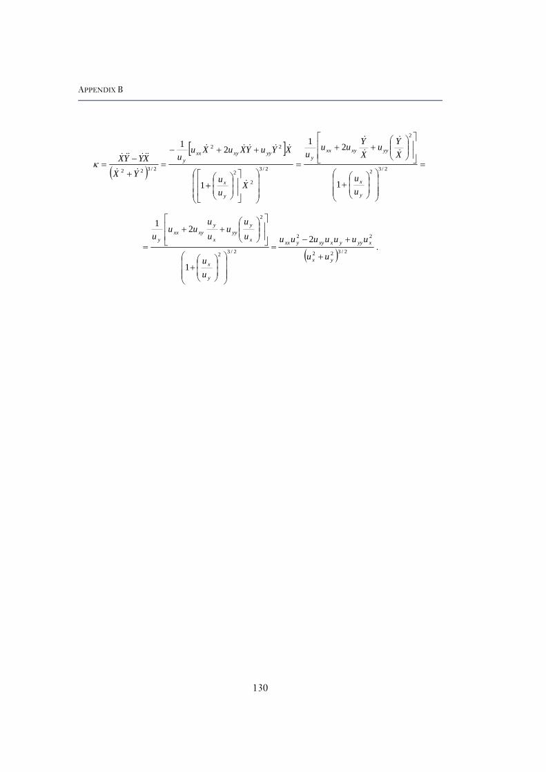
APPENDIX B
( )
[ ]=
⎟⎟⎟
⎠
⎞
⎜⎜⎜
⎝
⎛
⎟⎟⎠
⎞⎜⎜⎝
⎛+
⎥⎥⎦
⎤
⎢⎢⎣
⎡⎟⎟⎠
⎞⎜⎜⎝
⎛++
=
⎟⎟⎟
⎠
⎞
⎜⎜⎜
⎝
⎛
⎥⎥
⎦
⎤
⎢⎢
⎣
⎡
⎟⎟⎠
⎞⎜⎜⎝
⎛+
++−
=+
−= 2/32
2
2/3
2
2
22
2/322
1
21
1
21
y
x
yyxyxxy
y
x
yyxyxxy
uu
XYu
XYuu
u
Xuu
XYuYXuXuu
YX
XYYX&
&
&
&
&
&&&&&
&&
&&&&&&κ
( ) 2/322
22
2/32
2
2
1
21
yx
xyyyxxyyxx
y
x
x
yyy
x
yxyxx
y
uu
uuuuuuu
uu
uu
uuu
uuu
+
+−=
⎟⎟⎟
⎠
⎞
⎜⎜⎜
⎝
⎛
⎟⎟⎠
⎞⎜⎜⎝
⎛+
⎥⎥
⎦
⎤
⎢⎢
⎣
⎡
⎟⎟⎠
⎞⎜⎜⎝
⎛++
= .
130

131