Experiments in the Coordinated Control

of an Underwater Arm/Vehicle System

Timothy W. McLain� Stephen M. Rocky Michael J. Leez

Abstract

The addition of manipulators to small autonomous underwater vehicles (AUVs) can pose signi�cant control

challenges due to hydrodynamic interactions between the arm and the vehicle. Experiments conducted at the

Monterey Bay Aquarium Research Institute (MBARI) using the OTTER vehicle have shown that dynamical

interactions between an arm and a vehicle can be very signi�cant. For the experiments reported in this paper, a

single-link \arm" was mounted on OTTER. Tests showed that for 90-degree, two-second repetitive slews of the

arm, the vehicle would move as much as 18 degrees in roll and 14 degrees in yaw when no vehicle control was

applied.

Using a new, highly accurate model of the arm/vehicle hydrodynamic interaction forces, which was developed

as part of this research, a coordinated arm/vehicle control strategy was implemented. Under this model-based

approach, interaction forces acting on the vehicle due to arm motion were predicted and fed into the vehicle

controller. Using this method, station-keeping capability was greatly enhanced. Errors at the manipulator end

point were reduced by over a factor of six when compared to results when no control was applied to the vehicle

and by a factor of 2.5 when compared to results from a standard independent arm and vehicle feedback control

approach. Using the coordinated-control strategy, arm end-point settling times were reduced by a factor three

when compared to those obtained with arm and vehicle feedback control alone. These dramatic performance

improvements were obtained with only a �ve-percent increase in total applied thrust.

Key Words and Phrases

� underwater vehicle control

� underwater manipulator hydrodynamics

� underwater manipulator modeling

� underwater manipulator control

�Department of Mechanical Engineering, 242 CB, Brigham Young University, Provo, UT 84602, tmclain@et.byu.eduyDepartment of Aeronautics and Astronautics, 250 Durand Building, Stanford University, Stanford, CA 94305,

rock@sun-valley.stanford.eduzMonterey Bay Aquarium Research Institute, 160 Central Avenue, Paci�c Grove, CA 93950, lemi@mbari.org

� coordinated control

� vehicle and manipulator control

� underwater vehicle experiments

1 Introduction

For users of remotely operated vehicles (ROVs), manipulators have become a valuable tool for performing a wide

variety of tasks, from scienti�c sampling to maintenance and construction of underwater structures. Unlike ROVs,

which tend to be quite stable statically, many smaller underwater vehicles have reduced static stability due to the

small separation distance between their centers of mass and buoyancy. Also, for vehicles designed to travel e�ciently

through the water, the requirement for a small frontal area often limits the achievable static stability. The addition

of manipulators to the vehicle makes control of the system more di�cult because of the large hydrodynamic forces

acting on the arm as it moves through the water. Hydrodynamic forces on the arm couple into the vehicle system,

increasing the di�culty of regulating the position and attitude of the vehicle.

With the advent and implementation of higher levels of autonomy in the control of underwater robotic systems, it

is becoming possible to move faster, and hence the relevance of hydrodynamic coupling is increased further. Today's

advanced manipulator systems are typically tele-operated, using a passive \master" arm to control the underwater

\slave" robot arm. These systems, are limited in a fundamental way by the skill, coordination, and endurance of the

human operator. High-speed, precise motion is precluded by the limitations of the human/machine interface.

Human/machine interfaces incorporating increased autonomy, such as Task-Level Control [Wang et al., 1993], are

capable of providing commands which exploit the full capabilities of manipulators for quick, precise motions. As the

human operator is relieved of low-level control responsibilities, the limitations on system performance shift to the

control systems implemented in place of the human. To enable high-performance control of a manipulator end point

from a free-swimming vehicle base, low-level control systems that deal e�ectively with the complex hydrodynamics

of fast motion must be developed. The development and implementation of such a controller is the focus of this

paper.

A common work scenario for an underwater robot on a science mission is to perform a task, such as picking up

a rock, sampling a biological specimen from the water column, or moving a science instrument, while holding the

position and attitude of the vehicle �xed or \on station." Such tasks are examples of jobs where the station-keeping

control of the vehicle is very important. By using control to keep the vehicle motionless, not only is the manipulation

made easier, but the challenge of visually tracking the desired work scene is made less burdensome as well.

Station keeping is made di�cult due to the presence of disturbances in the ocean environment such as those due

to currents or tether forces. In the research presented here, the disturbance addressed is the large hydrodynamic

coupling force generated as the arm moves through the water. If precise positioning of the manipulator end point is

required, even relatively small motions at moderate speeds can have signi�cant degrading e�ects.

2

For the coordinated arm/vehicle control experiments discussed in this paper, a single-link arm was mounted on

the OTTER vehicle, which is shown in Figure 1 and discussed in Section 3. Under the coordinated-control approach,

the vehicle feedback controller was augmented with information about the hydrodynamic interaction forces between

the arm and the vehicle. This information was produced using a very accurate model (developed during this work)

of the hydrodynamic forces acting on a single-link arm. Although the single-link arm is quite simple mechanically,

hydrodynamically it is quite complex due to the unsteady, three-dimensional ows developed as the arm moves.

Although it does not possess the functionality of a full manipulator, the single link allows testing and validation

of the coordinated-control concept. It was necessary to develop a more advanced model because many of the

unique hydrodynamic attributes of robotic motion (e.g., short unsteady swinging motions, radial- ow and tip- ow

e�ects, etc.) had not been addressed by previous models. As hydrodynamic models for manipulators increase in

sophistication to handle accurately multiple links and degrees of freedom, the control approach presented here can

be extended easily to accommodate these systems.

The end-point-positioning and station-keeping performance of di�erent controllers was tested by commanding

the vehicle to maintain station while moving the arm from one position to another and then back to the original

position. This point-to-point positioning task was chosen as the evaluation experiment for this research for two

reasons. First, it is a generic task representative of other tasks of interest for an underwater system, such as sampling

or pick-and-place maneuvers. Second, successful point-to-point positioning of the manipulator end point requires

high-performance control of the entire arm/vehicle system. Such control is di�cult to achieve without compensating

for the hydrodynamic interaction forces explicitly in the control of the arm/vehicle system.

2 Background

Controlling underwater vehicles and robots to enable them to perform useful functions in the deep ocean rep-

resents a di�cult problem that has challenged researchers for many years. Lead by the initial work of Yoerger

and Slotine [Yoerger and Slotine, 1985], the application of sliding-mode control techniques to underwater vehicles

became an active area of interest [Dougherty et al., 1988][Anderson, 1992][Healey and Lienard, 1993]. The moti-

vation for using the sliding-mode approach is to enable robust control of the uncertain nonlinear vehicle system.

Other research focused on using adaptive or neural-network control methods to deal with uncertainty in the plant

model [Cristi et al., 1990][Goheen and Je�erys, 1990][Yuh, 1990][Yoerger and Slotine, 1991].

In the underwater-vehicle community, two theoretical e�orts are of direct relevance to the coordinated arm/vehicle

control approach taken in this research. In the work of Mahesh, Yuh, and Lakshmi [Mahesh et al., 1991], an adaptive

controller for coordinating vehicle and arm motion was proposed. The arm and vehicle were considered as a single

unit and an adaptive controller was developed for the whole system. This required a discrete-time approximation to

the full nonlinear arm/vehicle dynamics to be implemented in the control. The success of the approach is dependent

on the controller's ability to adapt accurately to rapidly changing hydrodynamic coe�cients. The approach has been

demonstrated using only a computer simulation of the planar motion of a vehicle. Experimental validation of the

3

e�ectiveness of their approach has not been demonstrated.

In a second, related e�ort, Koval [Koval, 1994] proposed a model-based feedforward control approach for the

stabilization of an underwater manipulation robot. In this work, the computational feasibility of a real-time hy-

drodynamic model implementation was addressed. Few implementation details were provided. No simulation or

experimental results were given.

Several recent papers have addressed the modeling of underwater robotic systems [L�evesque and Richard, 1994]

[McMillan et al., 1994][Tarn et al., 1995]. The focus of these papers is the e�cient simulation of underwater vehicles

and manipulators with many degrees of freedom. The models presented assume that drag and added-mass coe�cients

are constant. The latter two papers give an approach for calculating an estimate of the added-mass coe�cient, but do

not suggest a value for the drag coe�cient. L�evesque does not include added-mass or other acceleration terms in his

formulation, but suggests a value of 1.1 for the drag coe�cient. None of these models were validated experimentally.

Experimental results from this research have shown that for typical robotic motions, that the drag and added-mass

coe�cients of a swinging circular cylinder are not constant, but state-dependent functions of how far the cylinder

has traveled.

Unlike the references presented here, the focus of this paper is not on increasing robustness or adapting to existing

uncertainty, but rather on improving system performance by exploiting detailed knowledge of the system dynamics.

The approach taken here involves augmenting the existing vehicle feedback control with information based on a

fundamental physical understanding of the manipulator hydrodynamics, in a way that bene�ts the control of the

entire system. To achieve good results, this approach requires an accurate model of the manipulator hydrodynamics.

In this paper, the coordinated-control approach is described and experimental validation is given.

3 Experimental Apparatus

The work presented here was performed as part of a joint research program between the Stanford University Aerospace

Robotics Laboratory (ARL) and the Monterey Bay Aquarium Research Institute (MBARI). To enable experimen-

tal research in the ARL/MBARI program, a small underwater vehicle has been developed. OTTER (an Ocean

Technologies Test-bed for Engineering Research) is described brie y below, while further detail can be found in

[Wang et al., 1996].

For the arm/vehicle coordinated-control experiments presented in this paper, a single-link arm was mounted on

the OTTER vehicle. Experiments were carried out in the MBARI test tank located in Moss Landing, California.

The tank is 12 m in diameter and 4 m deep. The OTTER vehicle is about 2.1 m long, 0.95 m wide, and 0.45 m tall

and weighs about 145 kg in air. A photograph of the vehicle with the arm mounted is shown in Figure 1. The main

structural element of the vehicle is a 0.36 m diameter by 1.25 m long aluminum pressure housing which contains the

on-board computers and sensors. Two 0.12 m diameter housings of the same length contain NiCad batteries that

provide approximately 750 W-h of power. The battery modules are mounted underneath the main housing.

The pressure housings are surrounded by eight ducted thrusters which provide propulsion to the vehicle. Each

4

thruster housing contains its own commutation electronics and microcontroller that allow the motor to be current or

velocity controlled. All components are mounted to a welded stainless-steel frame which surrounds the main housing

and runs the length of the vehicle. The vehicle is covered by a streamlined �berglass shell. Additional buoyancy is

provided by �berglass-covered redwood blocks stored within the shell. Because the shell is free ooding, the e�ective

mass and inertia of the robot underwater are signi�cantly higher than in air.

The arm used for the arm/vehicle control experiments was 7.1 cm in diameter and 1.0 m long. This length was

chosen because it has roughly the same e�ective length as the prototype manipulator that has been designed for

OTTER when it is in a nominal operating con�guration. The arm was mounted from the fore-port corner of the

vehicle frame and tilted down at an angle of 60 degrees from the horizontal (see Figure 1). This con�guration was

chosen because it places the arm in the region most likely to be the workspace of a future manipulator. With the arm

mounted in this way, all of the vehicle degrees of freedom were a�ected by the forces generated as the arm moved.

In order to control the position and attitude of the vehicle, a variety of sensors were used. The horizontal (x; y)

position of the vehicle was measured using SHARPS, an acoustic long-baseline positioning system. The depth (z)

of the vehicle was sensed using a pressure transducer. Measurements of pitch and roll were provided by a dual-axis

inclinometer. Heading was measured using a ux-gate compass. Solid-state gyros were used to provide pitch, roll,

and yaw angular rates. Each of these sensors is commercially available.

The computer hardware used for this research consisted of a UNIX-based Sun workstation networked to a VME-

based real-time computer system. The real-time computer hardware consisted of a two 68040-based single-board

computers (on separate VME chassis) and a 16-channel, 12-bit analog input board housed on board the vehicle and

a 68030-based single-board computer at the control station. One 68040 board was used for vehicle control, while

the other was used for arm control. Communication to the arm motor was done at 31.25 kBaud through a serial

connection.

The real-time control software was developed in C++ for use under ControlShell [Rea, 1992], a software framework

for real-time systems, which runs on top of the VxWorks operating system [Win, 1993].

4 Approach

Dynamically Coordinated Control

The central idea of dynamically coordinated control is to take advantage of physical understanding of system dynamics

explicitly in the control of the arm/vehicle system. In the context of the control problem addressed here, this physical

understanding is embodied in an accurate model of the manipulator hydrodynamic forces. Under the coordinated-

control approach, hydrodynamic and inertial forces generated from the motion of the arm are modeled in real time

as the motion progresses. Based on the predicted interaction forces, thrust commands are sent to the thrusters

to counteract the forces generated by the arm motion. In this way, the control of the arm and the vehicle are

\coordinated." The experimental results presented in this paper demonstrate the validity of this coordinated-control

approach for the arm and the vehicle.

5

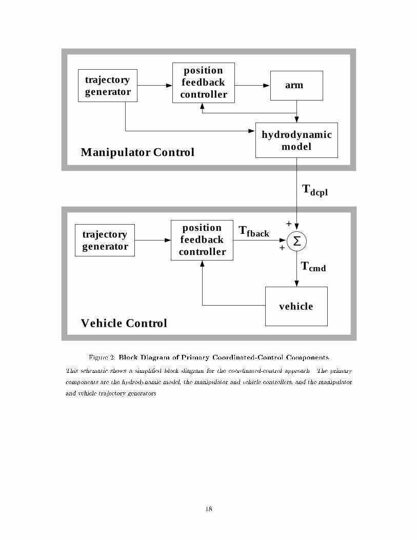
Figure 2 shows a simpli�ed schematic diagram of the coordinated-control strategy. The main control components

are the hydrodynamic model, the arm controller, the vehicle controller, the arm trajectory generator, and the vehicle

trajectory generator. For the station-keeping experiments of this paper, the vehicle trajectory generator supplied

zero-reference commands for each of the vehicle degrees of freedom. The control approach presented here was

developed with the availability of an accurate hydrodynamic model in mind. The primary bene�t of this model-

based control approach was the performance increase achieved by e�ectively eliminating one of the main disturbances

on the system. Using the modeling approach presented here to predict the hydrodynamic forces has the additional

bene�t of maintaining high reliability and low cost | no additional sensors are required.

Hydrodynamic Model

The experimental validation of the coordinated-control approach of this paper was enabled, in part, by the devel-

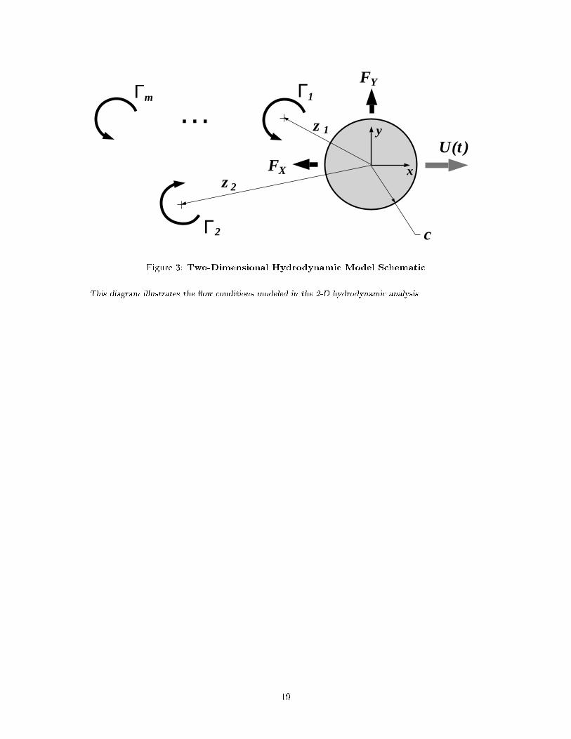
opment of a very accurate hydrodynamic model for the in-line forces1 acting on a circular cylinder rotating about

its end. The theoretical foundation of this model is a two-dimensional analysis of the ow of an incompressible,

inviscid uid over a cylinder undergoing unsteady motions. The wake and feeding layers were modeled using discrete

vortices with independent positions, velocities, and strengths. The analysis ignores the e�ects of skin drag, which are

negligible for the manipulator motions considered. Figure 3 shows a schematic representation of the 2-D cylinder.

The 2-D portion of this analysis is similar to that done by Sarpkaya [Sarpkaya, 1963, Sarpkaya and Garrison, 1963]

for a stationary cylinder immersed in a moving uid. Further details of the model can be found in [McLain, 1995].

The two-dimensional analysis resulted in the following equation for the acting hydrodynamic in-line force:

FX = Cm(s=D) � ��D2

4

dU

dt+ Cd(s=D) �

1

2�DU2: (1)

The key outcome of this analysis was that for a cylinder undergoing constant acceleration motions, it was found

that the state-dependent hydrodynamic drag and added-mass coe�cients, Cd and Cm, were functions of how far the

cylinder had traveled only.

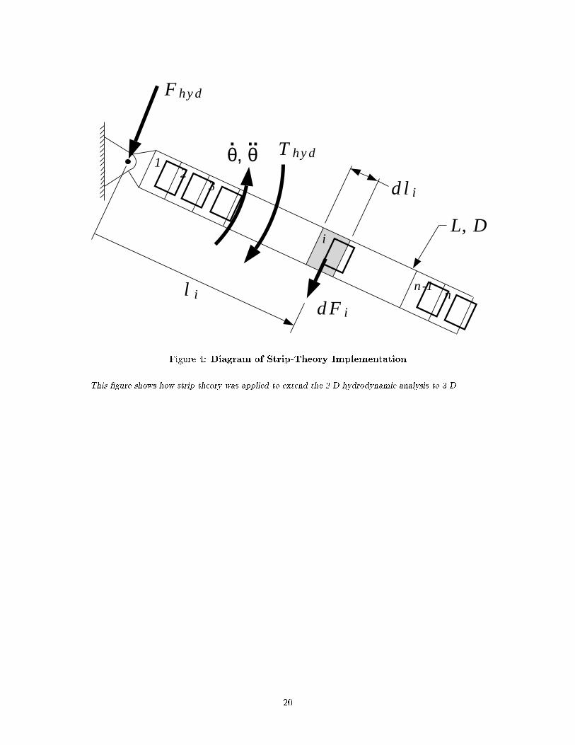
Using a standard strip-theory approach, the 2-D analysis was extended to three dimensions. This approach is

diagrammed in Figure 4. The forces acting on a thin segment of the arm were calculated using a form of Equation 1:

dFi = Cmi(si=D) � �

�D2

4lidli�� + Cdi(si=D) �

1

2�Dl2i dlij

_�j _�: (2)

The hydrodynamic in-line torque and force acting at the hub were found using the following simple relations:

dTi = lidFi (3)

Thyd =nXi=1

dTi (4)

1The net hydrodynamic force acting on the cross section of a cylinder is often viewed as the vector sum of the in-line forces and the

transverse (lift) forces. In-line forces, which act in the plane of the cylinder's motion, are due to drag and added-mass e�ects. Transverse

forces, which act normal to the plane of motion, are caused by the shedding of vortices into the wake.

6

Fhyd =

nXi=1

dFi (5)

where n was the number of segments used in the model.

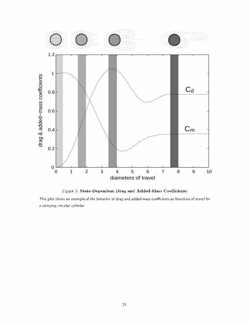
Extensive measurements of forces and torques acting on the arm were used to identify the state-dependent

behavior of Cd and Cm. Flow visualization studies were also conducted to gain insight into the behavior of the

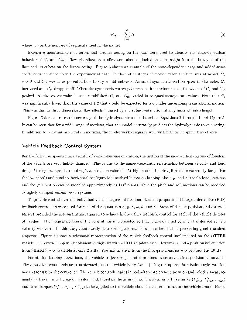
ow and its e�ects on the forces acting. Figure 5 shows an example of the state-dependent drag and added-mass

coe�cients identi�ed from the experimental data. In the initial stages of motion when the ow was attached, Cd

was 0 and Cm was 1, as potential- ow theory would indicate. As small symmetric vortices grew in the wake, Cd

increased and Cm dropped o�. When the symmetric vortex pair reached its maximum size, the values of Cd and Cm

peaked. As the vortex wake became established, Cd and Cm settled in to quasi-steady-state values. Note that Cd

was signi�cantly lower than the value of 1.2 that would be expected for a cylinder undergoing translational motion.

This was due to three-dimensional ow e�ects induced by the rotational motion of a cylinder of �nite length.

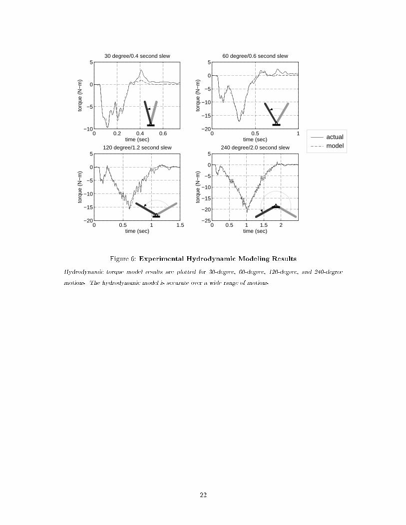
Figure 6 demonstrates the accuracy of the hydrodynamic model based on Equations 2 through 4 and Figure 5.

It can be seen that for a wide range of motions, that the model accurately predicts the hydrodynamic torque acting.

In addition to constant acceleration motions, the model worked equally well with �fth-order spline trajectories.

Vehicle Feedback Control System

For the fairly low speeds characteristic of station-keeping operation, the motion of the independent degrees of freedom

of the vehicle are very lightly damped. This is due to the signed-quadratic relationship between velocity and uid

drag. At very low speeds, the drag is almost non-existent. At high speeds the drag forces are extremely large. For

the low speeds and nominal horizontal con�guration involved in station keeping, the x; y; and z translational motions

and the yaw motion can be modeled approximately as 1=s2 plants, while the pitch and roll motions can be modeled

as lightly damped second-order systems.

To provide control over the individual vehicle degrees of freedom, classical proportional-integral-derivative (PID)

feedback controllers were used for each of the quantities x, y, z, �, �, and . State-of-the-art position and attitude

sensors provided the measurements required to achieve high-quality feedback control for each of the vehicle degrees

of freedom. The integral portion of the control was implemented so that it was only active when the desired vehicle

velocity was zero. In this way, good steady-state-error performance was achieved while preserving good transient

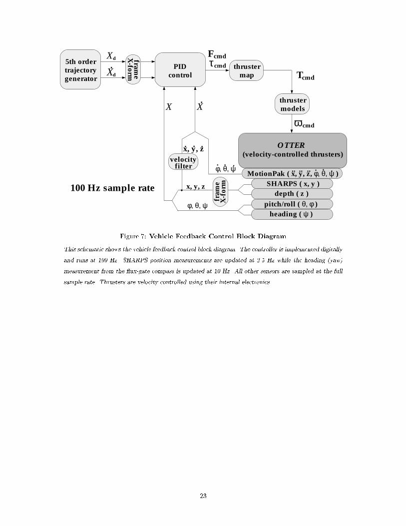
response. Figure 7 shows a schematic representation of the vehicle feedback control implemented on the OTTER

vehicle. The control loop was implemented digitally with a 100 Hz update rate. However, x and y position information

from SHARPS was available at only 2.5 Hz. Yaw information from the ux-gate compass was produced at 10 Hz.

For station-keeping operations, the vehicle trajectory generator produces constant desired-position commands.

These position commands are transformed into the vehicle-body frame (using the appropriate Euler-angle rotation

matrix) for use by the controller. The vehicle controller takes in body-frame-referenced position and velocity measure-

ments for the vehicle degrees of freedom and, based on the errors, produces a vector of three forces (F xcmd ; F

ycmd ; F

zcmd)

and three torques (�xcmd ; �ycmd ; �

zcmd) to be applied to the vehicle about its center of mass in the vehicle frame. Based

7

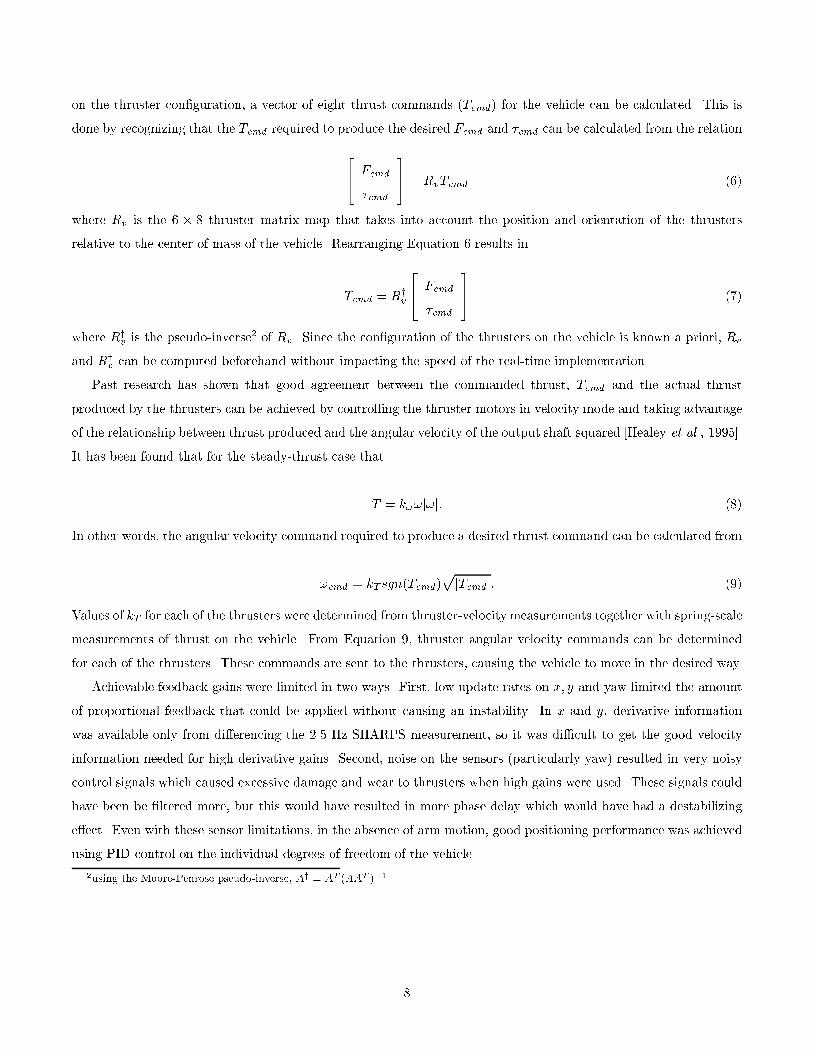
on the thruster con�guration, a vector of eight thrust commands (Tcmd) for the vehicle can be calculated. This is

done by recognizing that the Tcmd required to produce the desired Fcmd and �cmd can be calculated from the relation

24 Fcmd

�cmd

35 = RvTcmd (6)

where Rv is the 6 � 8 thruster matrix map that takes into account the position and orientation of the thrusters

relative to the center of mass of the vehicle. Rearranging Equation 6 results in

Tcmd = Ryv

24 Fcmd

�cmd

35 (7)

where Ryv is the pseudo-inverse2 of Rv. Since the con�guration of the thrusters on the vehicle is known a priori, Rv

and Ryv can be computed beforehand without impacting the speed of the real-time implementation.

Past research has shown that good agreement between the commanded thrust, Tcmd and the actual thrust

produced by the thrusters can be achieved by controlling the thruster motors in velocity mode and taking advantage

of the relationship between thrust produced and the angular velocity of the output shaft squared [Healey et al., 1995].

It has been found that for the steady-thrust case that

T = k!!j!j: (8)

In other words, the angular velocity command required to produce a desired thrust command can be calculated from

!cmd = kT sgn(Tcmd)pjTcmd j: (9)

Values of kT for each of the thrusters were determined from thruster-velocity measurements together with spring-scale

measurements of thrust on the vehicle. From Equation 9, thruster angular velocity commands can be determined

for each of the thrusters. These commands are sent to the thrusters, causing the vehicle to move in the desired way.

Achievable feedback gains were limited in two ways. First, low update rates on x; y and yaw limited the amount

of proportional feedback that could be applied without causing an instability. In x and y, derivative information

was available only from di�erencing the 2.5 Hz SHARPS measurement, so it was di�cult to get the good velocity

information needed for high derivative gains. Second, noise on the sensors (particularly yaw) resulted in very noisy

control signals which caused excessive damage and wear to thrusters when high gains were used. These signals could

have been be �ltered more, but this would have resulted in more phase delay which would have had a destabilizing

e�ect. Even with these sensor limitations, in the absence of arm motion, good positioning performance was achieved

using PID control on the individual degrees of freedom of the vehicle.

2using the Moore-Penrose pseudo-inverse, Ay = AT (AAT )�1

8

Arm Feedback Control System

For the single link, the in-line hydrodynamic forces, though nonlinear and somewhat uncertain, provided damping and

stability to the arm dynamics. Because of the well-damped dynamic characteristics of the arm, high position feedback

gains were achievable. Using straightforward implementation of classical control methods, very good position control

was attained.

Figure 8 shows a schematic block diagram of the arm controller implemented for the experiments described in

this paper. This implementation takes advantage of the 1 kHz, high-gain velocity feedback controller internal to the

motor electronics. By controlling the arm motor in \velocity control" mode, the arm actuator behaved as a velocity

source.

A �fth-order trajectory generator was used to provide smooth desired commands to the controller. Desired velocity

commands direct from the trajectory generator were sent to the motor as feedforward signals. A proportional position

feedback loop was closed around the internal velocity feedback loop to provide control of the arm joint angle �. The

sample rate was limited to 230 Hz by the achievable serial communication bandwidth between the VME cage and

the 68HC11 microcontroller in the motor housing.

Coordinated-Control Implementation

The coordinated-control approach implemented here involved augmenting existing independent arm and vehicle con-

trollers with information about their dynamic interaction to produce improved control of the system. Figure 9 shows

a schematic representation of the coordinated-control approach implemented on the OTTER system. The coordi-

nating information between the two systems came from the manipulator hydrodynamic model and the decoupling

thrust commands it generated.

Implementation Assumptions

The essential pieces of information necessary for implementation of the single-link manipulator hydrodynamic model

developed and described above are the position, velocity, and acceleration of the link relative to the water. In

implementing this approach, four key assumptions were made:

1. Vehicle motions are small and do not contribute signi�cantly to the net motion of the manipulator relative to

the water.

2. Desired arm-joint acceleration is a good approximation of the actual joint acceleration.

3. The water through which the arm is moving is still.

4. Transverse (lift) forces are insigni�cant in comparison to the in-line forces.

Under the condition that the vehicle and arm controllers are functioning as intended, the �rst two assumptions

are reasonable and valid. The bene�t of the �rst assumption is an increase in the control bandwidth due both to

9

a reduction in computational complexity and to a decrease in the amount of information passed over the limited-

bandwidth communication link between the arm and the vehicle. The bene�t of the second assumption (which is

standard for many model-based robot controllers) is that measurements of individual joint accelerations are not

required. The third assumption is valid for the tests reported here: In the large MBARI tank, uid motion is

due solely to thruster discharge which does not impinge on the arm. The validity of the fourth assumption has

been demonstrated experimentally at the ARL [McLain, 1995]. For the apparatus used and the types of motions

considered here, strong periodic vortex shedding did not become well-established, hence transverse (lift) forces are

comparatively very small.

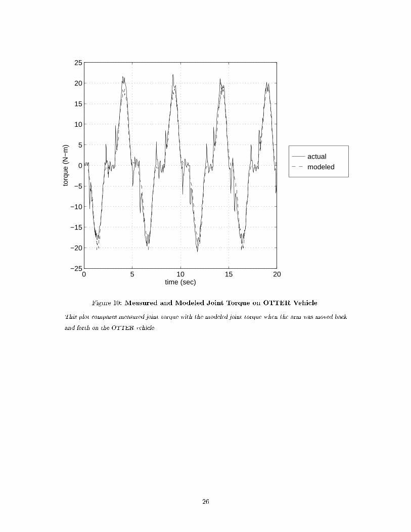
Figure 10 shows the hydrodynamic model performance under the assumptions outlined above. The agreement

between the measured arm-joint torque and the modeled arm-joint torque was quite good. Some errors existed at the

beginning and end of arm trajectories due to accelerations, caused by joint exibility, which were not incorporated

into the model when the desired acceleration signal was used. Errors during the middle of the trajectory (near the

torque peaks) were due primarily to vehicle motions which were not included in the model. In spite of the simplifying

assumptions made, it can be seen that good modeling accuracy was maintained.

Implementation Description

Feedback controllers were applied to the arm and vehicle as described above. In addition, the hydrodynamic model

and decoupling control connection were added to complete the coordinated-control implementation as shown in

Figure 9. To provide the rate information required for the model, the arm position signal was pseudo-di�erentiated

using a digital �lter. Position information came directly from the motor encoder, while the desired acceleration signal

was used to provide the required acceleration information.

The hydrodynamic model was implemented as described above. The output of the model was a vector of three

forces (F xhyd ; F

yhyd ; F

zhyd ) and three torques (�xhyd ; �

yhyd ; �

zhyd ) acting about the base of the arm joint. These were the

forces and torques required to counteract the forces generated by the motion of the arm. As with the feedback control,

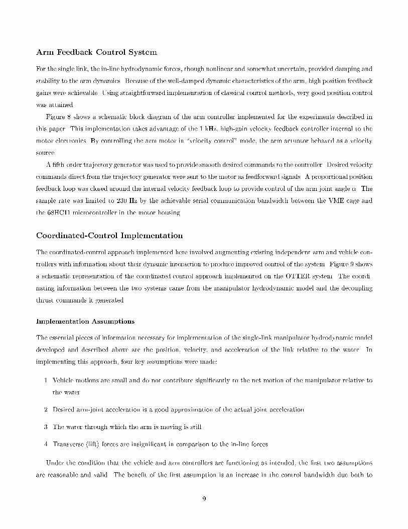
a thruster con�guration map was used to determine the required decoupling control commands to the thrusters, Tdcpl ,

to counteract the hydrodynamic coupling forces:

24 Fhyd

�hyd

35 = RaTdcpl : (10)

Tdcpl = Rya

24 Fhyd

�hyd

35 (11)

Ra was the 6� 8 thruster matrix map that took into account the position and orientation of the thrusters relative

to the base of the arm.

The vector Tdcpl of decoupling thruster commands was sent to the vehicle controller 60 times per second over an

Ethernet connection between the arm and vehicle card cages. These decoupling commands were summed directly

with the feedback commands, Tfback , to produce the the total thrust command to be sent to the thrusters, Tcmd .

10

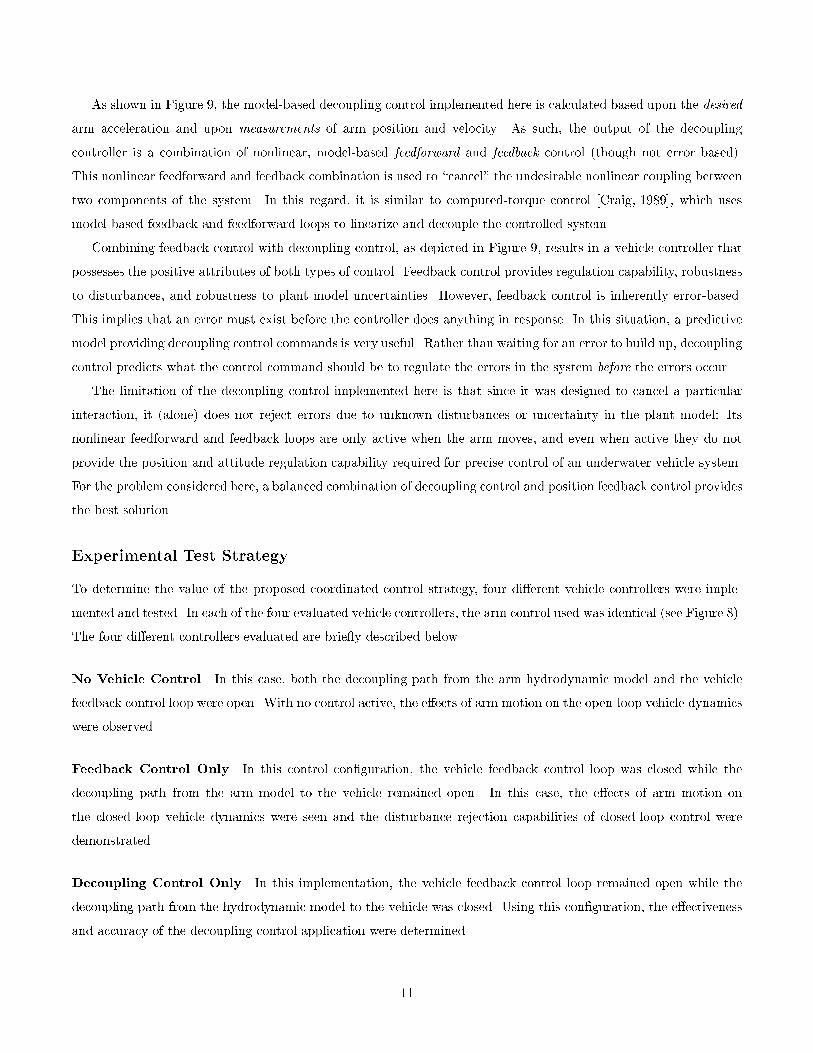
As shown in Figure 9, the model-based decoupling control implemented here is calculated based upon the desired

arm acceleration and upon measurements of arm position and velocity. As such, the output of the decoupling

controller is a combination of nonlinear, model-based feedforward and feedback control (though not error based).

This nonlinear feedforward and feedback combination is used to \cancel" the undesirable nonlinear coupling between

two components of the system. In this regard, it is similar to computed-torque control [Craig, 1989], which uses

model-based feedback and feedforward loops to linearize and decouple the controlled system.

Combining feedback control with decoupling control, as depicted in Figure 9, results in a vehicle controller that

possesses the positive attributes of both types of control. Feedback control provides regulation capability, robustness

to disturbances, and robustness to plant model uncertainties. However, feedback control is inherently error-based.

This implies that an error must exist before the controller does anything in response. In this situation, a predictive

model providing decoupling control commands is very useful. Rather than waiting for an error to build up, decoupling

control predicts what the control command should be to regulate the errors in the system before the errors occur.

The limitation of the decoupling control implemented here is that since it was designed to cancel a particular

interaction, it (alone) does not reject errors due to unknown disturbances or uncertainty in the plant model: Its

nonlinear feedforward and feedback loops are only active when the arm moves, and even when active they do not

provide the position and attitude regulation capability required for precise control of an underwater vehicle system.

For the problem considered here, a balanced combination of decoupling control and position feedback control provides

the best solution.

Experimental Test Strategy

To determine the value of the proposed coordinated-control strategy, four di�erent vehicle controllers were imple-

mented and tested. In each of the four evaluated vehicle controllers, the arm control used was identical (see Figure 8).

The four di�erent controllers evaluated are brie y described below.

No Vehicle Control In this case, both the decoupling path from the arm hydrodynamic model and the vehicle

feedback control loop were open. With no control active, the e�ects of arm motion on the open-loop vehicle dynamics

were observed.

Feedback Control Only In this control con�guration, the vehicle feedback control loop was closed while the

decoupling path from the arm model to the vehicle remained open. In this case, the e�ects of arm motion on

the closed-loop vehicle dynamics were seen and the disturbance rejection capabilities of closed-loop control were

demonstrated.

Decoupling Control Only In this implementation, the vehicle feedback control loop remained open while the

decoupling path from the hydrodynamic model to the vehicle was closed. Using this con�guration, the e�ectiveness

and accuracy of the decoupling control application were determined.

11

Feedback with Decoupling Control In this case, both the vehicle feedback control loop and the decoupling path

from the arm model were closed. In this control con�guration, the performance bene�ts of combining the decoupling

control, which provides predictive coordination between the motion of the arm and control of the vehicle, with the

vehicle feedback control, which provides robustness to disturbances and uncertainty, were tested.

The Feedback Control Only test case, along with the No Vehicle Control case, provide performance baselines

against which the Feedback with Decoupling Control approach are compared.

5 Experimental Results

This section presents results from the coordinated arm/vehicle control experiments. Data from two di�erent types

of tests are presented | multiple-swing motions and single-swing motions of the arm. In Figures 11 through 18,

data from experiments where the arm was swung back and forth between two positions multiple times are shown.

In Figures 19 through 21, data are presented where the arm was slewed a single time from one point to another.

Several di�erent types of data are presented including image sequences from video footage of the experiments,

vehicle error regulation data, arm end-point error data, and thruster usage data. Using these results comparisons

are drawn between the di�erent controller types. The results demonstrate the bene�ts of both feedback control and

decoupling control and their complementary attributes that result in the best control behavior when feedback and

decoupling control are combined.

Vehicle Station Keeping

Figures 12 through 15 show image sequences taken from video footage shot during arm/vehicle control experiments

with the OTTER vehicle. In each sequence, the images were taken at approximately one-second intervals during the

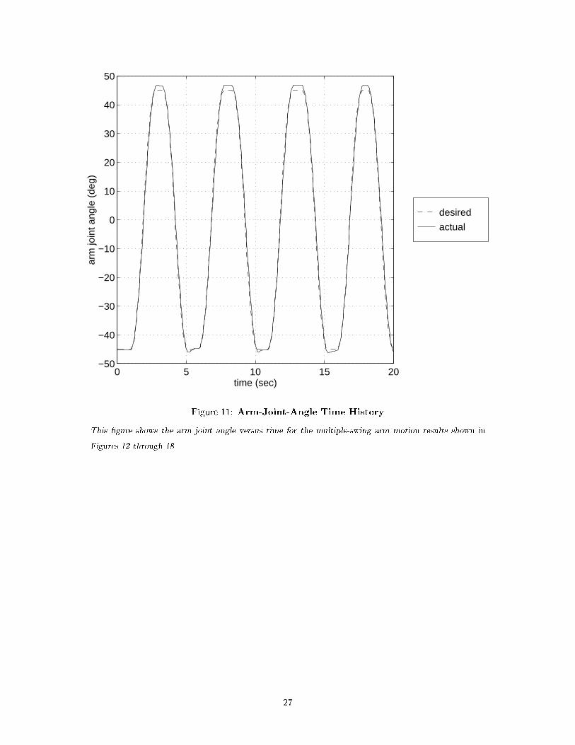
�rst three swings of the arm in a multiple-swing sequence. Figure 11 shows a typical time history of the arm joint

angle for the multiple-swing motions of the arm. The image sequences give a qualitative feel for the performance of

the di�erent controllers.

No Vehicle Control Figure 12 shows images taken for the No Vehicle Control case. It can be seen that the

open-loop roll mode of the vehicle was excited by the motion of the arm. Errors in roll were as large as 18 degrees

in both directions from the horizontal. A signi�cant error in yaw can also be observed. During this sequence, the

vehicle drifted about 15 degrees in yaw from its initial heading. These images demonstrate that the hydrodynamic

coupling forces involved in moving an arm at moderately fast speeds are very large and that they have a signi�cant

degrading e�ect on the station-keeping capability of a small, agile vehicle such as OTTER.

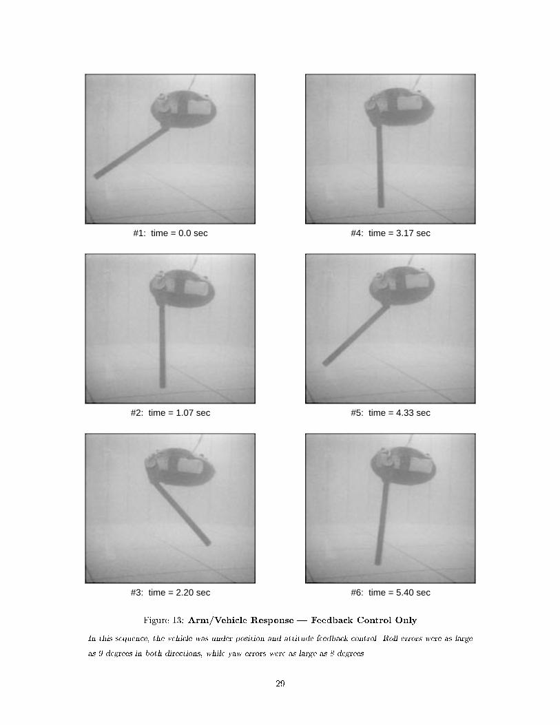
Feedback Control Only When compared with the No Vehicle Control case, the bene�ts of feedback control,

as shown in the sequences of Figure 13, are readily apparent. Errors in yaw and roll were reduced, but still very

signi�cant. The closed-loop roll mode, although much more damped than the open-loop mode, was still excited by

12

the arm motion. Roll motions were as large as nine degrees in both directions. The yaw angle of the vehicle varied

as much as eight degrees from its nominal position. While the bene�ts of closed-loop control are obvious from this

sequence of images, the disturbances introduced from the arm/vehicle coupling still resulted in substantial deviations

in the vehicle's position and attitude.

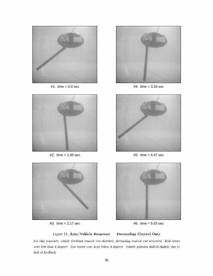
Decoupling Control Only The sequence of Figure 14 illustrates the performance of the controller in the Decou-

pling Control case. It can be seen that the in uence of the arm motion on the vehicle was greatly reduced. Errors

in roll and yaw were noticeably smaller. Since the application of the decoupling control did not perfectly cancel the

interaction forces, the open-loop roll mode was excited slightly by the combination of arm and thruster forces acting.

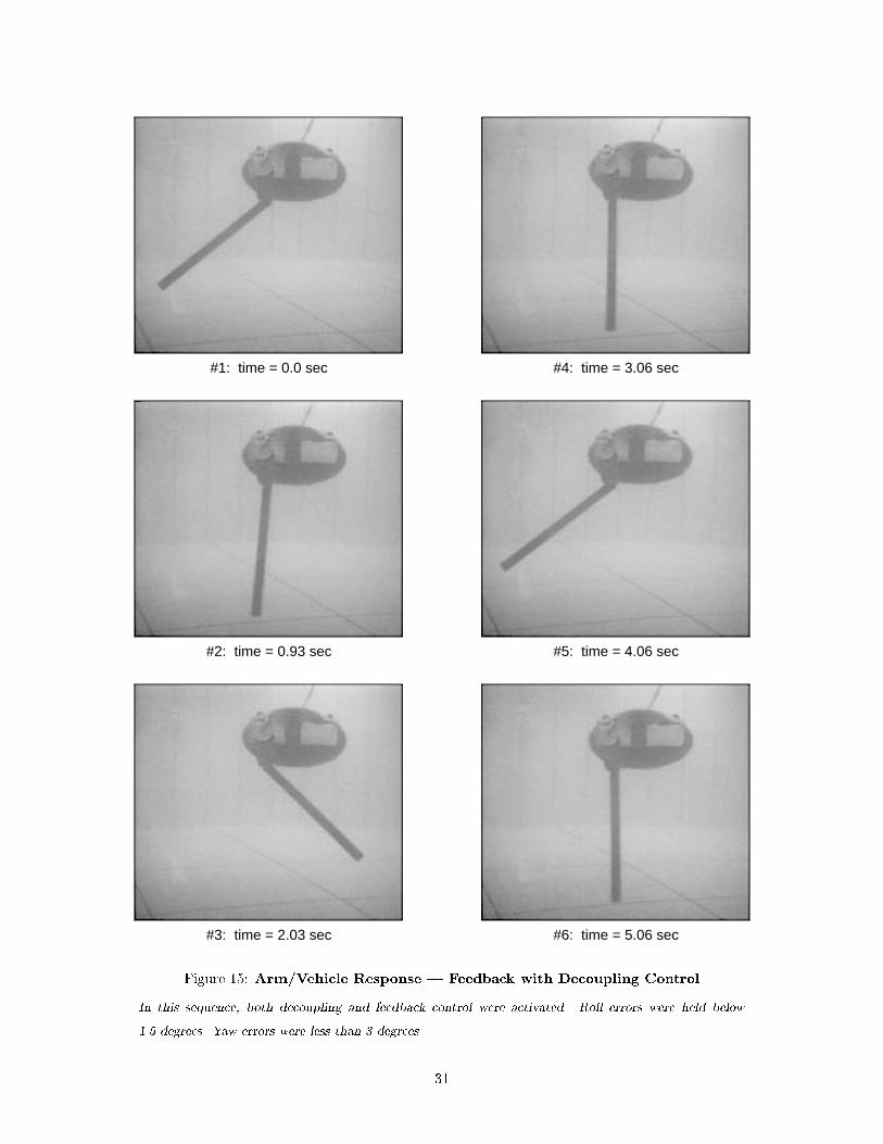
Feedback with Decoupling Control Figure 15 shows the performance results obtained using the Feedback with

Decoupling Control approach. As with the Decoupling Control Only case, the hydrodynamic interaction forces were

largely canceled by the decoupling component of the control. The advantage of adding the feedback control was that

the remaining errors from the inexact decoupling control were further reduced by the error regulation of the feedback

control. With the addition of feedback control, robustness to system uncertainty was provided and the tendency of

the vehicle to drift o� station was eliminated. These bene�ts are demonstrated clearly in a more quantitative way

in the following sections.

As a �nal comparison of the station-keeping performance of the di�erent vehicle controllers, selected vehicle roll

and yaw angle data are presented. In this particular application, errors in roll and yaw were the largest contributors

to the arm end-point error, especially in the cases of No Vehicle Control and Feedback Control Only.

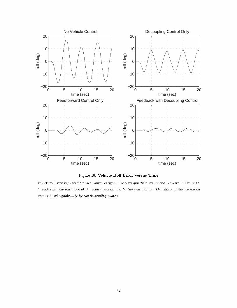
Vehicle Roll Error Figure 16 shows time histories of vehicle roll error data for each of the four controller types

considered. With no control e�ort, roll errors were very large (between �18 degrees) as the open-loop roll mode of

the vehicle was excited. The addition of feedback control improved the roll error regulating performance, but the

errors were still signi�cant (between �9 degrees). Decoupling control alone e�ectively countered much of the roll

moment generated from the arm motion. In this case, decoupling control allowed the vehicle to respond to arm

interaction forces before signi�cant attitude errors were induced. Further improvement was realized when decoupling

and feedback control were combined. Peak roll errors were limited to less than 1.5 degrees in this case.

Vehicle Yaw Error Time histories of vehicle yaw error for the di�erent controllers are shown in Figure 17.

When no feedback or decoupling control was applied, the vehicle heading angle drifted signi�cantly from its nominal

position. Unlike the roll and pitch attitude degrees of freedom, the yaw degree of freedom has no passive restoring

force inherent to its open-loop dynamics. Because of this the yaw degree of freedom was fully dependent on feedback

control to prevent drifting due to disturbances or uncertainty in the plant model. When feedback control alone was

applied, the tendency to drift was reduced, but the closed-loop dynamics of the yaw controller became apparent. As

the controller attempted to reject the yaw disturbance, it caused the vehicle to oscillate signi�cantly in response (up

to 9 degrees error). When decoupling control only was applied, the yaw disturbance due to arm motion e�ectively was

13

canceled resulting in much smaller yaw errors. With feedback and decoupling control combined, the yaw errors were

again small. Yaw errors were roughly three times smaller for the Decoupling Only and Feedback with Decoupling

cases than for the Feedback Only case.

Summary For each of the degrees of freedom of the vehicle, the best error regulation results were obtained when

both decoupling and feedback control were combined. The decoupling control e�ectively canceled most of the

dynamical coupling between the arm and the vehicle. Much of the remaining coupling e�ect was eliminated by

the feedback control. The feedback control also provided for the rejection of other disturbances (e.g., tether forces,

currents) and robustness to uncertainties in the plant.

Arm End-Point Positioning Performance

While not sensed and controlled directly in these experiments, arm end-point position error is a useful indicator of the

quality of the performance of the arm/vehicle controller. End-point position data were generated by post-processing

vehicle position and attitude and arm position measurements based on the kinematic con�guration of the system.

Data sampling on the vehicle controller and arm controller was synchronously triggered to allow correlation of arm

and vehicle data in time.

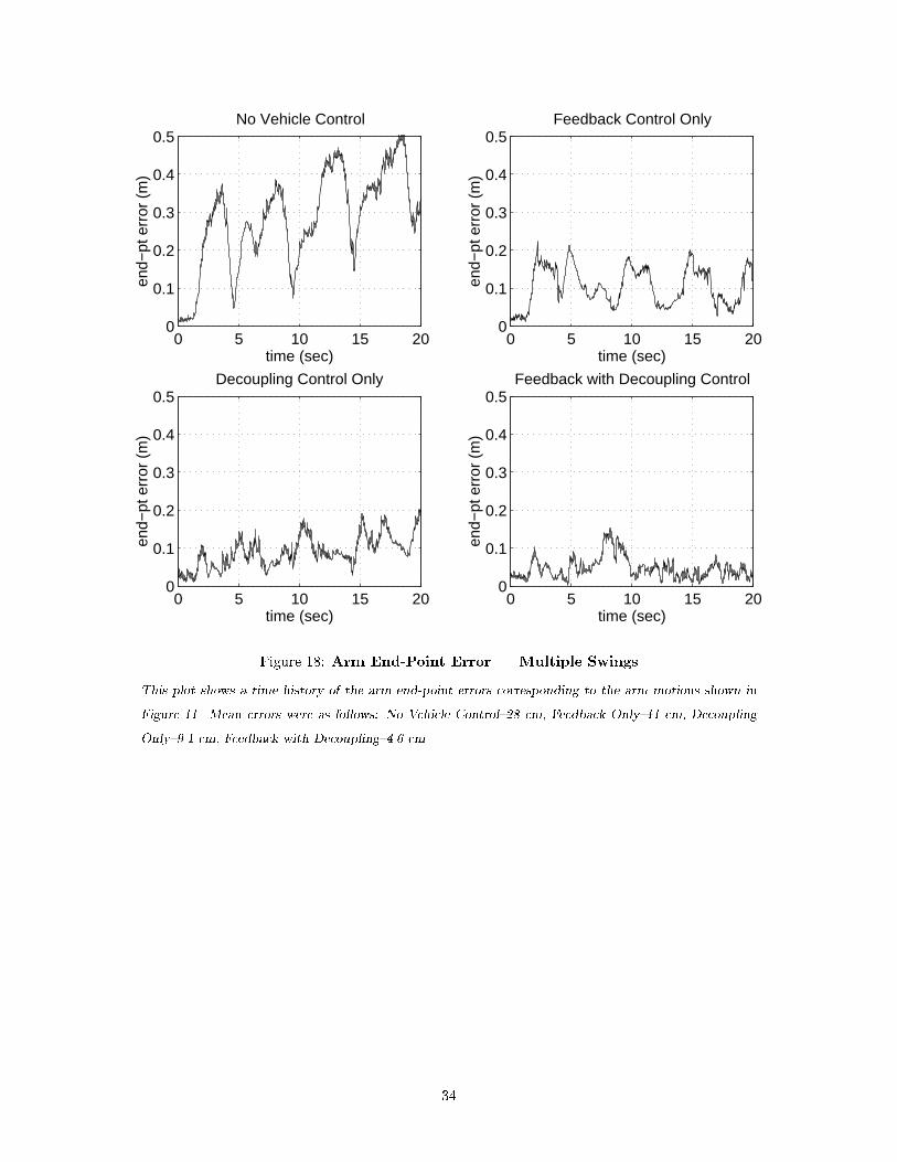
For the multiple-swing motions of the arm, Figure 18 shows time histories of the arm end-point error for the four

controllers tested. The mean end-point errors were calculated to be 28 cm for the No Vehicle Control case, 11 cm

for the Feedback Control Only case, 9.1 cm for the Decoupling Control Only case, and 4.6 cm for the Feedback with

Decoupling Control case. It can be seen that with combined decoupling and feedback control, that the end-point

errors were reduced by a factor of six when compared with the No Vehicle Control case and a factor of 2.5 when

compared to the Feedback Control Only case. In the Feedback with Decoupling Control case, where end-point errors

were smallest, a more signi�cant portion of the error can be attributed to the arm joint-angle error. During the arm

slews, joint tracking errors were typically around 2 to 3 cm.

Arm End-Point Settling-Time Performance

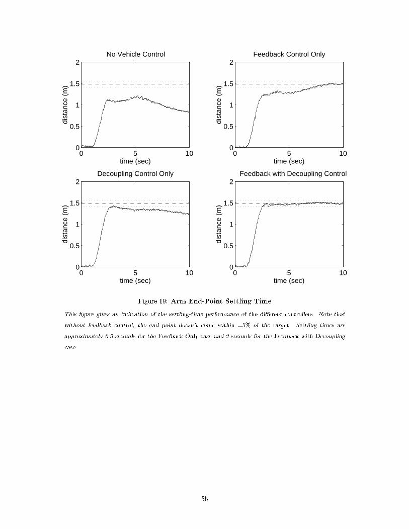
Figure 19 shows plots of the distance of the arm end point from the desired target for the four di�erent controllers.

This data was obtained by slewing the arm through 90 degrees in two seconds. For the slews considered, the distance

traveled by the end point was about 1.5 m. Here settling time is de�ned as the time required to stay within �ve

percent (of the total distance traveled) of the target | in this case �7:5 cm.

These settling-time plots demonstrate the importance of the feedback component of the vehicle control. Without

feedback, the arm end point either fails to come within �ve percent of the target (as in the No Vehicle Control case)

or it fails to remain within the �ve-percent error bound around the target point (as in the Decoupling Control Only

case).

In the Feedback Control Only case, the time required to settle to within �ve percent of the target was about 6.5

seconds. As the arm moved, signi�cant errors in roll, yaw, x, and y resulted. Coming and staying within the error

14

bound required these errors to be reduced which took a substantial amount of time.

In the Feedback with Decoupling Control case, the observed settling time was about two seconds. This represents

an improvement of over three times compared to the settling time of the Feedback Control case. Because the vehicle

stayed on station, the settling time corresponded directly to the duration of the slew.

Thruster Usage

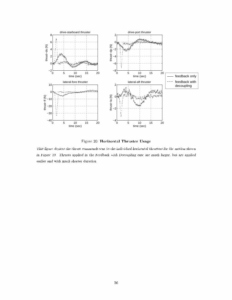
Horizontal Thrusters Figure 20 shows thruster responses for each of the horizontal thrusters on the vehicle for

the Feedback Only and Feedback with Decoupling cases. For each thruster, it can be seen that the Feedback with

Decoupling thrusts spiked up to comparatively large values during the slew, but then settled to very small values

almost immediately after the slew ended. On the other hand, for the Feedback Only case it can be seen that the

thruster commands were much smaller initially, but that the thrusters �red over much longer durations. Long after

the thrusters had essentially shut o� in the Feedback with Decoupling case, they continued to �re in the Feedback

Only case in an e�ort to regulate the errors in the system. These plots illustrate the predictive capability of the

decoupling control, which in each case leads the feedback control in responding to the arm motion.

Note that the largest thrust command by far came from the lateral-fore thruster. This makes sense physically

since the lateral-fore thruster was positioned very close to the base of the arm joint and the lateral forces generated

by the arm were very large. The responsibility for countering these forces fell largely upon the lateral-fore thruster.

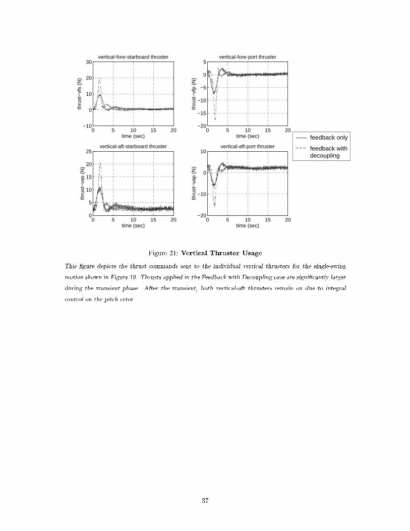
Vertical Thrusters Figure 21 shows thruster responses for each of the vertical thrusters on the vehicle for the

Feedback Only and Feedback with Decoupling cases. As with the horizontal thrusters, the vertical Feedback with

Decoupling thrust commands spiked up to large values during the arm motion to compensate for the interaction

forces generated. Unlike the horizontal thrusters, the vertical thrusters responded fairly quickly to the roll errors

introduced in the Feedback Only case. Notice that in both control cases the vertical-aft thrusters remained on well

after the completion of the arm motion. This was due to the integral control acting to zero the pitch error of the

vehicle.

Comparison of Thruster Usage Two useful indicators of thruster usage are peak thrust applied and the total

thrust3 applied over the 20-second duration shown. Peak thrusts give a good indication of worst-case instantaneous

demand on the thrusters, while total thrust usage gives a better indication the total thrust (and hence battery power)

required over the duration of the test. For the thruster data shown in Figures 20 and 21, the peak thrusts were 1.8

to 2.7 times larger in the Feedback with Decoupling case, with the exception of the lateral-fore thruster where it was

�ve times larger. While the peaks are much higher due to the decoupling component of the command coming from

the hydrodynamic model, the thrust durations were shorter for the Feedback with Decoupling case. This is re ected

in the relative values of the total thrust used in each control case: Only �ve percent more total thrust was used in

the Feedback with Decoupling case than for the Feedback Only case.

3Total thrust was calculated by summing the absolute values of the thrusts applied over the duration of the test, while subtracting

out any DC components. This is analogous to evaluating the expressionR

jTcmd j dt.

15

The key result of this comparison is that for a slight increase in total thrust used, a very substantial performance

improvement was realized (see Figure 19). This was accomplished by taking advantage of knowledge of the system

dynamics and coordinating the control in a sensible way.

6 Conclusions

In this paper, an intuitively straightforward approach developed for the coordinated control of an underwater

arm/vehicle system has been described in detail. Relevant background information has been presented along with de-

tailed discussion of the control system implementation. Experiments demonstrated that the hydrodynamic coupling

forces between an arm and a vehicle can be very signi�cant, resulting in large disturbances to the station-keeping

control of the vehicle. Experimental results showed that substantial performance improvements can be realized in

the control of an underwater arm/vehicle system by incorporating model-based information about the hydrodynamic

coupling into the control of the system. Tracking errors at the manipulator end point were typically reduced by over

a factor of six using the coordinated control approach when compared to the vehicle with no control applied and

by a factor of 2.5 when compared to the standard approach of independent arm and vehicle feedback controllers.

Using the approach presented here, settling times at the manipulator end point were also reduced by over three times

when compared to the values obtained using feedback control alone. It is important to note that these dramatic

performance improvements were achieved with only a �ve-percent increase in total control e�ort.

7 Acknowledgments

This research was supported by the Monterey Bay Aquarium Research Institute, ONR Contract N0014-92-J-1943,

and NASA Contract NCC 2-333. This research has bene�ted greatly from the contributions of the other participants

in the ARL/MBARI research program: Dick Burton, Howard Wang, Rick Marks, David Miles, Glen Sapilewski,

Kortney Leabourne, and Steve Fleischer.

16

Figure 1: OTTER Vehicle With Single-Link Arm

This photo shows the OTTER vehicle with the single-link manipulator mounted. The single-link manip-

ulator is 7.1 cm in diameter and 1.0 m long, while the vehicle is 2.1 m long, 0.95 m wide and 0.45 m

tall.

17

Tcmd

vehicle

dcplT

hydrodynamicmodel

trajectorygenerator

positionfeedbackcontroller

arm

TfbackΣ+

+trajectorygenerator

positionfeedbackcontroller

Manipulator Control

Vehicle Control

Figure 2: Block Diagram of Primary Coordinated-Control Components

This schematic shows a simpli�ed block diagram for the coordinated-control approach. The primary

components are the hydrodynamic model, the manipulator and vehicle controllers, and the manipulator

and vehicle trajectory generators.

18

U(t)z 1

z2

1Γ

2Γ

mΓ

FX

FY

c

…x

y

Figure 3: Two-Dimensional Hydrodynamic Model Schematic

This diagram illustrates the ow conditions modeled in the 2-D hydrodynamic analysis.

19

⋅

θ, θ. ..

12

3

n-1n

i

⋅

⋅⋅⋅

⋅dl i

l idF i

L, D

F hyd

T hyd

Figure 4: Diagram of Strip-Theory Implementation

This �gure shows how strip-theory was applied to extend the 2-D hydrodynamic analysis to 3-D.

20

Cd

Cm

0 1 2 3 4 5 6 7 8 9 100

0.2

0.4

0.6

0.8

1

1.2

diameters of travel

drag

& a

dded

−mas

s co

effic

ient

s

Figure 5: State-Dependent Drag and Added-Mass Coe�cients

This plot shows an example of the behavior of drag and added-mass coe�cients as functions of travel for

a swinging circular cylinder.

21

0 0.2 0.4 0.6−10

−5

0

5

time (sec)

torq

ue (

N−m

)

30 degree/0.4 second slew

0 0.5 1−20

−15

−10

−5

0

5

time (sec)

torq

ue (

N−m

)

60 degree/0.6 second slew

0 0.5 1 1.5−20

−15

−10

−5

0

5

time (sec)

torq

ue (

N−m

)

120 degree/1.2 second slew

0 0.5 1 1.5 2−25

−20

−15

−10

−5

0

5

time (sec)

torq

ue (

N−m

)

240 degree/2.0 second slew

actualmodel

Figure 6: Experimental Hydrodynamic Modeling Results

Hydrodynamic torque model results are plotted for 30-degree, 60-degree, 120-degree, and 240-degree

motions. The hydrodynamic model is accurate over a wide range of motions.

22

5th ordertrajectorygenerator

PIDcontrol

Xd

X.d

thrustermap

thrustermodels

OTTER(velocity-controlled thrusters)

MotionPak ( x, y, z, φ, θ, ψ )...... .. .

SHARPS ( x, y )depth ( z )

pitch/roll ( θ, φ )heading ( ψ )

frame

X-form

fram

eX

-for

m

φ, θ, ψ.. .

φ, θ, ψ

x, y, z

velocityfilter

x, y, z. . .

X X.

Tcmd

Fcmdcmdτ

cmdω

100 Hz sample rate

Figure 7: Vehicle Feedback Control Block Diagram

This schematic shows the vehicle feedback control block diagram. The controller is implemented digitally

and runs at 100 Hz. SHARPS position measurements are updated at 2.5 Hz while the heading (yaw)

measurement from the ux-gate compass is updated at 10 Hz. All other sensors are sampled at the full

sample rate. Thrusters are velocity controlled using their internal electronics.

23

αd

αd.

5th ordertrajectorygenerator

Σ

Σ

kp

αcmd. arm motor

(velocitycontrolled)

encod

er

+

+

-

+α

230 Hz sample rate

Figure 8: Arm Feedback Control Block Diagram

This schematic shows the arm feedback control block diagram. The controller is implemented digitally at

230 Hz. The arm motor was velocity controlled by a 1 kHz, high-gain feedback controller implemented

on the 68HC11 microcontroller that is part of the motor commutation electronics.

24

Manipulator Control

hydrodynamicmodel

Fhydhydτ

αd

αd..αd.5th order

trajectorygenerator

Σ

Σ

kp

αcmd. arm motor

(velocitycontrolled)

encod

er

+

+

-

+α

ratefilter

α. thruster

map

5th ordertrajectorygenerator

PIDcontrol

Xd

X.d

thrustermap

thrustermodels

OTTER(velocity-controlled thrusters)

MotionPak ( x, y, z, φ, θ, ψ )...... .. .

SHARPS ( x, y )depth ( z )

pitch/roll ( θ, φ )heading ( ψ )

frame

X-form

fram

eX

-for

m

φ, θ, ψ.. .

φ, θ, ψ

x, y, z

velocityfilter

x, y, z. . .

X X.

Vehicle Control

TdcplTfback

++Tcmd

Fcmdcmdτ

cmdω

Σ

230 Hz sample rate

100 Hz sample rate

60 Hz comm. rate

Figure 9: Coordinated-Control Implementation Block Diagram

This schematic shows the block diagram of the coordinated-control scheme as implemented on the OTTER

vehicle. The arm controller runs in one VME cage at 230 Hz, while the vehicle controller runs in a second

VME cage at 100 Hz. The hydrodynamic model information is sent from the arm controller to the vehicle

controller over an Ethernet connection at 60 Hz.

25

actual

modeled

0 5 10 15 20−25

−20

−15

−10

−5

0

5

10

15

20

25to

rque

(N

−m

)

time (sec)

Figure 10: Measured and Modeled Joint Torque on OTTER Vehicle.

This plot compares measured joint torque with the modeled joint torque when the arm was moved back

and forth on the OTTER vehicle.

26

desired

actual

0 5 10 15 20−50

−40

−30

−20

−10

0

10

20

30

40

50

time (sec)

arm

join

t ang

le (

deg)

Figure 11: Arm-Joint-Angle Time History

This �gure shows the arm joint angle versus time for the multiple-swing arm motion results shown in

Figures 12 through 18.

27

#1: time = 0.0 sec #4: time = 3.07 sec

#2: time = 0.93 sec #5: time = 4.03 sec

#3: time = 2.07 sec #6: time = 5.33 sec

Figure 12: Arm/Vehicle Response | No Vehicle Control

For this sequence, all control commands to the thrusters were disabled. The vehicle rolled as much as

18 degrees in both directions from its nominal horizontal position. In yaw, the vehicle rotated about

15 degrees from its initial heading angle.

28

#1: time = 0.0 sec #4: time = 3.17 sec

#2: time = 1.07 sec #5: time = 4.33 sec

#3: time = 2.20 sec #6: time = 5.40 sec

Figure 13: Arm/Vehicle Response | Feedback Control Only

In this sequence, the vehicle was under position and attitude feedback control. Roll errors were as large

as 9 degrees in both directions, while yaw errors were as large as 8 degrees.

29

#1: time = 0.0 sec #4: time = 3.33 sec

#2: time = 1.00 sec #5: time = 4.47 sec

#3: time = 2.17 sec #6: time = 5.53 sec

Figure 14: Arm/Vehicle Response | Decoupling Control Only

For this sequence, vehicle feedback control was disabled, decoupling control was activated. Roll errors

were less than 3 degrees. Yaw errors were kept below 4 degrees. Vehicle position drifted slightly due to

lack of feedback.

30

#1: time = 0.0 sec #4: time = 3.06 sec

#2: time = 0.93 sec #5: time = 4.06 sec

#3: time = 2.03 sec #6: time = 5.06 sec

Figure 15: Arm/Vehicle Response | Feedback with Decoupling Control

In this sequence, both decoupling and feedback control were activated. Roll errors were held below

1.5 degrees. Yaw errors were less than 3 degrees.

31

0 5 10 15 20−20

−10

0

10

20No Vehicle Control

roll

(deg

)

time (sec)0 5 10 15 20

−20

−10

0

10

20Decoupling Control Only

roll

(deg

)

time (sec)

0 5 10 15 20−20

−10

0

10

20Feedforward Control Only

roll

(deg

)

time (sec)0 5 10 15 20

−20

−10

0

10

20Feedback with Decoupling Control

roll

(deg

)

time (sec)

Figure 16: Vehicle Roll Error versus Time

Vehicle roll error is plotted for each controller type. The corresponding arm motion is shown in Figure 11.

In each case, the roll mode of the vehicle was excited by the arm motion. The e�ects of this excitation

were reduced signi�cantly by the decoupling control.

32

0 5 10 15 20−10

−5

0

5

10

15

20No Vehicle Control

yaw

(de

g)

time (sec)0 5 10 15 20

−10

−5

0

5

10

15

20Decoupling Control Only

yaw

(de

g)

time (sec)

0 5 10 15 20−10

−5

0

5

10

15

20Feedforward Control Only

yaw

(de

g)

time (sec)0 5 10 15 20

−10

−5

0

5

10

15

20Feedback with Decoupling Control

yaw

(de

g)

time (sec)

Figure 17: Vehicle Yaw Error versus Time

This �gure shows yaw error for each controller type tested. The corresponding arm motion is shown

in Figure 11. Yaw errors were roughly three times smaller for the Decoupling Only and Feedback with

Decoupling cases than for the Feedback Only case.

33

0 5 10 15 200

0.1

0.2

0.3

0.4

0.5

time (sec)

end−

pt e

rror

(m

)

No Vehicle Control

0 5 10 15 200

0.1

0.2

0.3

0.4

0.5

time (sec)

end−

pt e

rror

(m

)

Feedback Control Only

0 5 10 15 200

0.1

0.2

0.3

0.4

0.5

time (sec)

end−

pt e

rror

(m

)

Decoupling Control Only

0 5 10 15 200

0.1

0.2

0.3

0.4

0.5

time (sec)

end−

pt e

rror

(m

)

Feedback with Decoupling Control

Figure 18: Arm End-Point Error | Multiple Swings

This plot shows a time history of the arm end-point errors corresponding to the arm motions shown in

Figure 11. Mean errors were as follows: No Vehicle Control{28 cm, Feedback Only{11 cm, Decoupling

Only{9.1 cm, Feedback with Decoupling{4.6 cm.

34

0 5 100

0.5

1

1.5

2

time (sec)

dist

ance

(m

)

No Vehicle Control

0 5 100

0.5

1

1.5

2

time (sec)

dist

ance

(m

)

Feedback Control Only

0 5 100

0.5

1

1.5

2

time (sec)

dist

ance

(m

)

Decoupling Control Only

0 5 100

0.5

1

1.5

2

time (sec)

dist

ance

(m

)

Feedback with Decoupling Control

Figure 19: Arm End-Point Settling Time

This �gure gives an indication of the settling-time performance of the di�erent controllers. Note that

without feedback control, the end point doesn't come within �5% of the target. Settling times are

approximately 6.5 seconds for the Feedback Only case and 2 seconds for the Feedback with Decoupling

case.

35

0 5 10 15 20−2

0

2

4

6

8

time (sec)

thru

st−d

s (N

)

0 5 10 15 20−8

−6

−4

−2

0

2

time (sec)

thru

st−d

p (N

)

0 5 10 15 20−40

−30

−20

−10

0

10

time (sec)

thru

st−l

f (N

)

0 5 10 15 20−4

−2

0

2

time (sec)

thru

st−l

a (N

)

feedback only

feedback withdecoupling

drive-starboard thruster

lateral-aft thruster

drive-port thruster

lateral-fore thruster

Figure 20: Horizontal Thruster Usage

This �gure depicts the thrust commands sent to the individual horizontal thrusters for the motion shown

in Figure 19. Thrusts applied in the Feedback with Decoupling case are much larger, but are applied

earlier and with much shorter duration.

36

0 5 10 15 20−10

0

10

20

30

time (sec)

thru

st−

vfs

(N)

0 5 10 15 20−20

−15

−10

−5

0

5

time (sec)

thru

st−

vfp

(N)

0 5 10 15 200

5

10

15

20

25

time (sec)

thru

st−

vas

(N)

0 5 10 15 20−20

−10

0

10

time (sec)

thru

st−

vap

(N)

feedback only

feedback withdecoupling

vertical-fore-starboard thruster

vertical-aft-port thruster

vertical-fore-port thruster

vertical-aft-starboard thruster

Figure 21: Vertical Thruster Usage

This �gure depicts the thrust commands sent to the individual vertical thrusters for the single-swing

motion shown in Figure 19. Thrusts applied in the Feedback with Decoupling case are signi�cantly larger

during the transient phase. After the transient, both vertical-aft thrusters remain on due to integral

control on the pitch error.

37

References

[Anderson, 1992] Jamie M. Anderson. Model development and control of the autonomous benthic explorer. In

Proceedings of the Second International O�shore and Polar Engineering Conference, pages 468{472. International

Society of O�shore and Polar Engineers, June 1992.

[Craig, 1989] John J. Craig. Introduction to Robotics: Mechanics and Control. Addison-Wesley, 2nd edition, 1989.

[Cristi et al., 1990] Roberto Cristi, Fotis A. Papoulias, and Anthony J. Healey. Adaptive sliding mode control of

autonomous underwater vehicles in the dive plane. IEEE Journal of Oceanic Engineering, 15(3):152{160, 1990.

[Dougherty et al., 1988] Frank Dougherty, Tom Sherman, Gary Woolweaver, and Gib Lovell. An autonomous un-

derwater vehicle (AUV) ight control system using sliding mode control. In Oceans '88, pages 1265{1270. IEEE,

1988.

[Goheen and Je�erys, 1990] Kevin R. Goheen and E. Richard Je�erys. Multivariable self-tuning autopilots for au-

tonomous and remotely operated underwater vehicles. IEEE Journal of Oceanic Engineering, 15(3):144{151, 1990.

[Healey and Lienard, 1993] Anthony J. Healey and David Lienard. Multivariable sliding-mode control for au-

tonomous diving and steering of unmanned underwater vehicles. IEEE Journal of Oceanic Engineering, 18(3):327{

339, 1993.

[Healey et al., 1995] A. J. Healey, S. M. Rock, S. Cody, D. Miles, and J. P. Brown. Toward an improved understanding

of thruster dynamics underwater vehicles. IEEE Journal of Oceanic Engineering, 20(4):354{361, 1995. Accepted

for publication in the October 1995 issue.

[Koval, 1994] Elena V. Koval. Automatic stabilization system of underwater manipulation robot. In Oceans '94

Proceedings, pages I{807{I{812. IEEE, September 1994.

[L�evesque and Richard, 1994] Beno�t L�evesque and Marc J. Richard. Dynamic analysis of a manipulator in a uid

environment. International Journal of Robotics Research, 13(3):221{231, 1994.

[Mahesh et al., 1991] H. Mahesh, J. Yuh, and R. Lakshmi. A coordinated control of an underwater vehicle and

robotic manipulator. The Journal of Robotic Systems, 8(3):339{370, 1991.

[McLain, 1995] Timothy W. McLain. Modeling of Underwater Manipulator Hydrodynamics with Application to the

Coordinated Control of an Arm/Vehicle System. PhD thesis, Stanford University, August 1995. Also published as

SUDAAR 670.

[McMillan et al., 1994] Scott McMillan, David E. Orin, and Robert B. McGhee. E�cient dynamic simulation of an

unmanned underwater vehicle with a manipulator. In Proceedings of the International Conference on Robotics and

Automation, pages 1133{1140, 1994.

38

[Rea, 1992] Real-Time Innovations, Inc., 155A Mo�et Park Drive, Suite 111, Sunnyvale, CA 94089. ControlShell

User's Manual: A Real-time Software Framework, 4.2a edition, November 1992.

[Sarpkaya and Garrison, 1963] Turgut Sarpkaya and C. J. Garrison. Vortex formation and resistance in unsteady

ow. Journal of Applied Mechanics, pages 16{24, March 1963.

[Sarpkaya, 1963] Turgut Sarpkaya. Lift, drag, and added-mass coe�cients for a circular cylinder immersed in a

time-dependent ow. Journal of Applied Mechanics, pages 13{15, March 1963.

[Tarn et al., 1995] T.J. Tarn, G.A. Shoults, and S. Yang. Dynamical model for a free- oating underwater robotic

vehicle with an n-axis manipulator. In Proceedings of the U.S.{Portugal Workshop on Undersea Robotics and

Intelligent Control, Lisboa, March 1995.

[Wang et al., 1993] H. H. Wang, R. L. Marks, S. M. Rock, and M. J. Lee. Task-Based Control Architecture for an

Untethered, Unmanned Submersible. In Proceedings of the 8th Annual Symposium of Unmanned Untethered Sub-

mersible Technology, pages 137{147. Marine Systems Engineering Laboratory, Northeastern University, September

1993.

[Wang et al., 1996] Howard Wang, Stephen M. Rock, and Michael J. Lee. OTTER: The design and development of

an intelligent underwater robot. Journal of Autonomous Robots, 3:299{322, 1996.

[Win, 1993] Wind River Systems, Inc., 1010 Atlantic Avenue, Alameda, CA 94501-1147. VxWorks Programmer's

Guide 5.1, December 1993.

[Yoerger and Slotine, 1985] Dana R. Yoerger and Jean-Jaques E. Slotine. Robust trajectory control of underwater

vehicles. IEEE Journal of Oceanic Engineering, 10(4):462{470, 1985.

[Yoerger and Slotine, 1991] Dana R. Yoerger and Jean-Jaques E. Slotine. Adaptive sliding control of an experimental

underwater vehicle. In Proceedings of the International Conference on Robotics and Automation, pages 2746{2751.

IEEE, April 1991.

[Yuh, 1990] Junku Yuh. A neural net controller for underwater robotic vehicles. IEEE Journal of Oceanic Engineer-

ing, 15(3):161{166, 1990.

Authors

Timothy W. McLain received B.S. degree in 1986 and M.S. degree in 1987 in Mechanical Engineering from

Brigham Young University. From 1987 to 1989, he worked at the Center for Engineering Design at the University

of Utah, where he was involved in modeling and simulation of hydraulic and electromechanical actuation systems,

actuator and control system development, and force transducer design. From 1989 through 1995, Dr. McLain was a

Research Assistant in the Aerospace Robotics Laboratory at Stanford University. His Ph.D. research, which was done

39

in cooperation with the Monterey Bay Aquarium Research Institute, focused on the hydrodynamics of underwater

manipulators and the design of control systems for underwater vehicles and manipulators. Currently, Dr. McLain is

an Assistant Professor of Mechanical Engineering at Brigham Young University where his research interests center

on the control of hydraulic and pneumatic actuation systems.

StephenM. Rock received his S.B. and S.M. degrees in Mechanical Engineering from the Massachusetts Institute

of Technology in 1972, and the Ph.D. degree in Applied Mechanics from Stanford University in 1978. Dr. Rock joined

the Stanford faculty in 1988, and is now an Associate Professor in the department of Aeronautics and Astronautics.

Prior to joining the Stanford faculty, Dr. Rock led the Controls and Instrumentation Department of Systems Control

Technology, Inc. In his eleven years at SCT, he performed and led research in integrated control; fault detection,

isolation and accommodation; turbine engine modeling and control; and parameter identi�cation. Dr. Rock's current

research interests include the development and experimental validation of control approaches for robotic systems and

for vehicle applications. A major focus is both the high-level and low-level control of underwater robotic vehicles.

Michael J. Lee received his S.B. degree in Electrical Engineering form the Massachusetts Institute of Technology

in 1975 and the M.S. degree in Electrical Engineering from Stanford University in 1979. Mr. Lee joined the Hewlett

Packard Co. in 1976 and held several engineering and management positions including Department Manager of the

Control Systems Department at HP Laboratories. In 1987, Mr. Lee joined MBARI as one of its founders with the

position of Technical Director. Mr. Lee was an Adjunct Professor in Electrical Engineering at Boise State University

from 1977 through 1978, and is currently a Consulting Associate Professor at Stanford University.

40