experimental investigation of unstrained diffusion … · mesure´ a` l’aide d’un syste`me de...
TRANSCRIPT

POUR L'OBTENTION DU GRADE DE DOCTEUR ÈS SCIENCES
PAR
acceptée sur proposition du jury:
Prof. M. Deville, président du juryProf. P. Monkewitz, directeur de thèse
Prof. M. Matalon, rapporteur Dr Ph. Metzener, rapporteur
Prof. Ph. R. von Rohr, rapporteur
Experimental Investigation of Unstrained Diffusion Flames and their Instabilities
Etienne ROBERT
THÈSE NO 4249 (2008)
ÉCOLE POLYTECHNIQUE FÉDÉRALE DE LAUSANNE
PRÉSENTÉE LE 12 DÉCEMBRE 2008
À LA FACULTE SCIENCES ET TECHNIQUES DE L'INGÉNIEUR
LABORATOIRE DE MÉCANIQUE DES FLUIDES
PROGRAMME DOCTORAL EN MÉCANIQUE
Suisse2009


A Emma et Nils,
Merci!


v
Acknowledgments et remerciements
This thesis would not have been possible without a great number of people, their sup-port, their skills and their ideas. This page will certainlybe too short to express all ofmy gratitude, but I still wish to thank them properly.
First and foremost, the idea behind the burner used and developed in this thesisis the brainchild of my thesis supervisor, professor Peter Monkewitz. I would like toexpress my deep gratitude for giving me the opportunity to work on such an interestingproblem. His experimental instincts and considerable theoretical wisdom are the mainreasons I learned so much during this thesis, thank you Peter.
Peter also introduced me to professor Moshe Matalon, who wasof great help withthe theoretical side of the problem. His collaboration was extremely valuable in en-suring that our experimental realization was consistent with the theoretical approach tothe problem, and for that I am grateful.
None of the work presented here would have been possible without the financialsupport of the Swiss National Science Foundation under Grant 20020-108074.
Un grand merci aussi aux mecaniciens de l’atelier central qui ont avec tellementde talent transforme mes idees folles en realite. Merciparticulier a Bernard pour levolume considerable de travail qu’il a accompli sur ce projet, avec toujours une qualiteirreprochable. Merci a Marc pour avoir compris l’urgence de la situation quand c’etaisnecessaire. Merci a tous les autres pour les petits et les plus gros coups de pouce!
Merci aussi aux collegues qui font qu’autour d’une biere `a sat ou d’une glace surla terrasse, il est possible de deconnecter de cette thesel’espace d’un instant. Mercia ceux que j’ai cotoyes longtemps : Emeric, Richard et Radboud qui ont d’excellentecompagnie durant cette these, que ce soit pour le cote technique ou social. Je n’oubliepas les doctorants qui ont quitte le labo peu apres mon arrivee : Chris Pipe et en par-ticulier David Lo Jacono qui realisa la premiere version de l’experience utilisee danscette these. Merci aussi aux doctorants du labo d’a cote,en particuler Roland, Orestis etMarc-Antoine, sans qui les pause cafes se passeraient bientrop souvent en petit comitevu la modeste taille de notre labo.
Les visites regulieres et toujours agreables des membres de ma famille ont aussiete fort utiles pour garder le moral au fil de toute ses annees passees loin de mon petitcoin de pays. Une pensee toute particuliere pour mon papa Michel et mes deux petitsfreres Marc-Antoine et Pierre-Yves qui n’ont pas hesitea venir se graisser les mainsdans mon labo quand ils passent me voir en Suisse.
Finalement, je ne saurais passer sous silence le support indfectible que j’ai recu demon amour de toujours. Emma, merci infiniment pout tout, tu esla meilleure! Plusrecemment, les merveilleux sourires de mon fils Nils qui me tire les pantoufles quandj’ecris cette these ont ete une source de motivation incroyable.


vii
Abstract
In this thesis, thermal-diffusive instabilities are studied experimentally in diffusionflames. The novel species injector of a recently developed research burner, consistingof an array of hypodermic needles, which allows to produce quasi one-dimensional un-strained diffusion flames has been improved. It is used in a new symmetric design withfuel andoxidizer injected through needle arrays which allows to independently chooseboth the magnitude and direction of the bulk flow through the flame. A simplifiedtheoretical model for the flame position, the temperature and the species concentrationprofiles with variable bulk flow is presented which accounts for the transport propertiesof both reactants. The model results are compared to experiments with aCO2-dilutedH2-O2 flame using variable bulk flow and inert mixture composition.
The mixture composition throughout the burning chamber is monitored by massspectrometry. An elaborate calibration procedure has beenimplemented to account forthe variation of the mass spectrometer sensitivity as a function of the mixture composi-tion. The calibrated results allow theeffectivemixture strength of the diffusion flamesto be measured with a relative uncertainty of about 5 %.
In order to properly characterize the flame produced, the velocity and temperaturedistribution inside the burning chamber are measured. The resulting species concen-tration and temperature profiles are compared to the simplified theory and demonstratethat the new burner configuration produces a good approximation of the 1-D cham-bered diffusion flame, which has been used extensively for the stability analysis ofdiffusion flames. The velocity profiles are also used to quantify the residual stretchexperienced by the flame which is extremely low, below0.15 s�1. Hence, this new re-search burner opens up new possibilities for the experimental validation of theoreticalmodels developed in the idealized unstrained 1-D chamberedflame configuration.
The thermal-diffusive instabilities observed close to extinction are investigated ex-perimentally and mapped as a function of the Lewis numbers ofthe reactants. The useof a mixture of two inerts (helium and CO2) allows for the effect of a wide range ofLewis numbers to be studied. A cellular flame structure is observed in hydrogen flameswhen the Lewis numbers is relatively low with a typical cell size between7 and15 mm.The cell size is found to scale linearly with the diffusion length, in good agreement withtheoretical predictions. When the Lewis number is increased by using a higher heliumcontent in the dilution mixture, the instabilities observed are planar intensity pulsation.The use of methane allowed pulsating flames to be generated for a wide range of bulkvelocities and transport properties. The pulsating frequencies measured are in the0.7
to 11 Hz range and were found to scale linearly with a diffusion frequency defined asU22Dth multiplied by the square root of the Damkohler number. The experimental re-sults presented here are the first observations of thermal-diffusive instabilities in sucha low-strain flame. They constitute a unique dataset that canbe used to quantitativelyvalidate theoretical models on diffusion flame stability developed in the simplified one-dimensional configuration.
Keywords: Thermal-diffusive instability, unstrained, diffusion flame, experimental.


ix
Resume
L’utilisation d’un nouveau type the bruleur permet de produire des flammes de dif-fusion uni-dimensionelles et sans etirement. La nouveaute reside dans la maniereavec laquelle les especes reactives sont introduites dans le bruleur, au travers de cen-taines d’aiguilles hypodermiques. Une evolution du design est introduite dans laquellel’arrangement symetrique du systeme d’injection permetun controle independant surl’intensite et la direction de l’ecoulement moyen dans lachambre de combustion. Unmodele theorique simplifie tenant compte de l’ecoulement moyen variable est presentepour la position de flamme de meme que les profils de concentration et d’espece dansle bruleur. Les predictions de ce modele sont compares aux resultats experimentauxpour des flammes d’hydrogene et d’oxygene dilues dans du CO2.
La composition du melange de gaz present dans la chambre decombustion estmesure a l’aide d’un systeme de spectrometrie de masse.Une technique de calibrationsophistiquee a du etre mise au point pour compenser le changement de la sensibilitede l’instrument intervenant en fonction de la composition du melange mesure. Laflamme produite a aussi ete characterisee par la mesure des distributions de vitesse etde temperature dans le bruleur. Les profils de concentration et de temperature ainsiobtenus ont ete compares avec succes a la theorie simplifiee. Ceci demontre que laflamme produite est une bonne approximation de la configuration uni-dimensionellesimplifiee, qui est utilisee abondement dans le development de modeles theoriques surla stabilite des flammes de diffusion. Les profils de vitessepermettent egalement uneevaluation de l’etirement residuel subi par la flamme, qui est inferieur a0.15 s�1. Cenouveau type de bruleur de recherche ouvre de nombreuses possibilites de recherches,en particulier pour la validation experimentale de modeles theoriques sur la stabilitedes flammes de diffusion, developes en supposant une absence d’etirement dans laconfiguration uni-dimensionelle simlifiee.
Les instabilites thermo-diffusives formees a l’approche de l’extinction ont ete ob-servees et cartographiees en fonction des nombres de Lewis des especes utilisees.L’utilisation d’un melange de deux gaz inertes (helium etCO2) pour la dilution desespeces reactives a permis le balayage d’une large plage de nombres de Lewis. Unestructure de flamme cellulaire est observee pour les nombres de Lewis relativementfaibles, avec une taille de cellules comprise entre7 et 15 mm, evoluant lineairementavec la longueur characteristique de diffusion, conformement aux predictions theoriques.Quand le nombre de Lewis est augmente en utilisant une plus grande proportion d’heli-um dans le melange de dilution, les instabilites observees deviennent des oscillationsplannes de l’intensite de la reaction. L’utilisation du methane comme combustible apermis la production de flammes oscillantes sur une large plage de vitesse d’advectionet de propriete de transport du melange. Les frequencesde pulsation observees sontincluses dans l’intervalle de0.7 a11 Hz, et evoluent en fonction d’une frequence de dif-fusion definie commeU22Dth multipliee par la racine carree du nombre de Damkohler.Les resultats experimentaux d’instabilite thermo-diffusives presentes ici sont les pre-miers realises dans une telle flamme pratiquement depourvue d’etirement. Ils con-stituent une base de donnees unique permettant les premieres validations quantitativesdes modeles sur la stabilite des flammes de diffusion realises dans la configurationuni-dimensionnelle simplifiee.
Mots-cles: Instabilites thermo-diffusives, flamme de diffusion, etirement, etude exper-imentale.


Contents
1 Introduction 11.1 Chemically reacting flows . . . . . . . . . . . . . . . . . . . . . . . 11.2 Reaction-diffusion instabilities . . . . . . . . . . . . . . . . .. . . . 2
1.2.1 The study of thermal-diffusive (TD) instabilities . .. . . . . 51.2.2 The study of TD instabilities in diffusion flames . . . . .. . . 6
1.3 Objectives and scope of the thesis . . . . . . . . . . . . . . . . . . .71.4 Contributions . . . . . . . . . . . . . . . . . . . . . . . . . . . . . . 81.5 Thesis Outline . . . . . . . . . . . . . . . . . . . . . . . . . . . . . . 9
2 State of the art 112.1 Theoretical studies . . . . . . . . . . . . . . . . . . . . . . . . . . . 112.2 Experimental studies . . . . . . . . . . . . . . . . . . . . . . . . . . 142.3 Numerical methods . . . . . . . . . . . . . . . . . . . . . . . . . . . 16
3 Theoretical considerations 193.1 Simple one-dimensional model for the baseline flame . . . .. . . . . 19
3.1.1 Reaction-sheet approximation . . . . . . . . . . . . . . . . . 203.1.2 Model results . . . . . . . . . . . . . . . . . . . . . . . . . . 223.1.3 Adiabatic flame temperature . . . . . . . . . . . . . . . . . . 23
3.2 Stability considerations . . . . . . . . . . . . . . . . . . . . . . . . .243.2.1 The response curve . . . . . . . . . . . . . . . . . . . . . . . 243.2.2 Thermal-diffusive instabilities . . . . . . . . . . . . . . . .. 27
3.3 Numerical tools . . . . . . . . . . . . . . . . . . . . . . . . . . . . . 28
4 Experimental facilities and methods 314.1 The burners . . . . . . . . . . . . . . . . . . . . . . . . . . . . . . . 31
4.1.1 Mark I burner . . . . . . . . . . . . . . . . . . . . . . . . . . 324.1.2 Mark II burner . . . . . . . . . . . . . . . . . . . . . . . . . 35
4.2 Image Acquisition . . . . . . . . . . . . . . . . . . . . . . . . . . . . 394.2.1 Photography . . . . . . . . . . . . . . . . . . . . . . . . . . 394.2.2 Video . . . . . . . . . . . . . . . . . . . . . . . . . . . . . . 41
4.3 Velocity measurements . . . . . . . . . . . . . . . . . . . . . . . . . 414.3.1 Laser Doppler Anemometry (LDA) . . . . . . . . . . . . . . 424.3.2 Hot thermistor anemometry . . . . . . . . . . . . . . . . . . 42
4.4 Temperature measurements . . . . . . . . . . . . . . . . . . . . . . . 434.4.1 Temperature measurements with thermocouples . . . . . .. . 444.4.2 Probes fabrication . . . . . . . . . . . . . . . . . . . . . . . 444.4.3 Effective temperature . . . . . . . . . . . . . . . . . . . . . . 50
xi

xii CONTENTS
4.5 Gas mixtures preparation . . . . . . . . . . . . . . . . . . . . . . . . 51
5 Mixture composition measurements 555.1 The choice of experimental technique . . . . . . . . . . . . . . . .. 555.2 Mass spectrometry based PPA . . . . . . . . . . . . . . . . . . . . . 575.3 The instrument working principles . . . . . . . . . . . . . . . . . .. 57
5.3.1 Sampling . . . . . . . . . . . . . . . . . . . . . . . . . . . . 595.3.2 The ion source . . . . . . . . . . . . . . . . . . . . . . . . . 595.3.3 The mass analyzer . . . . . . . . . . . . . . . . . . . . . . . 615.3.4 The detectors . . . . . . . . . . . . . . . . . . . . . . . . . . 615.3.5 Control software . . . . . . . . . . . . . . . . . . . . . . . . 62
5.4 Mass spectrometer calibration . . . . . . . . . . . . . . . . . . . . .635.4.1 Built-in procedure . . . . . . . . . . . . . . . . . . . . . . . 635.4.2 Calibration over a wide concentration range . . . . . . . .. . 645.4.3 Results and discussion . . . . . . . . . . . . . . . . . . . . . 69
6 Burner characterization 736.1 Flame shape . . . . . . . . . . . . . . . . . . . . . . . . . . . . . . . 74
6.1.1 Flame parasitic curvature . . . . . . . . . . . . . . . . . . . . 756.1.2 Formation of convection cells . . . . . . . . . . . . . . . . . 76
6.2 Velocity measurements . . . . . . . . . . . . . . . . . . . . . . . . . 786.2.1 Injection layer . . . . . . . . . . . . . . . . . . . . . . . . . 786.2.2 Transverse velocity profiles . . . . . . . . . . . . . . . . . . 796.2.3 Residual strain . . . . . . . . . . . . . . . . . . . . . . . . . 81
6.3 Temperature measurements . . . . . . . . . . . . . . . . . . . . . . . 836.3.1 Temperature in the burning chamber . . . . . . . . . . . . . . 86
6.4 Species measurements . . . . . . . . . . . . . . . . . . . . . . . . . 866.4.1 Species transverse concentration profiles . . . . . . . . .. . 876.4.2 Species longitudinal concentration profiles . . . . . . .. . . 89
6.5 Flame position . . . . . . . . . . . . . . . . . . . . . . . . . . . . . 906.5.1 Virtual origin . . . . . . . . . . . . . . . . . . . . . . . . . . 906.5.2 Influence of bulk velocity . . . . . . . . . . . . . . . . . . . 936.5.3 Influence of Lewis number . . . . . . . . . . . . . . . . . . . 93
7 Experimental observation of TD instabilities 977.1 Stability and extinction limits . . . . . . . . . . . . . . . . . . . .. . 977.2 Mapping of the instabilities . . . . . . . . . . . . . . . . . . . . . . .1007.3 Cellular flames . . . . . . . . . . . . . . . . . . . . . . . . . . . . . 102
7.3.1 Observed instabilities . . . . . . . . . . . . . . . . . . . . . . 1027.3.2 Cell size scaling . . . . . . . . . . . . . . . . . . . . . . . . 105
7.4 Planar intensity pulsations . . . . . . . . . . . . . . . . . . . . . . .1077.4.1 Observed instabilities . . . . . . . . . . . . . . . . . . . . . . 1097.4.2 Pulsation frequency scaling . . . . . . . . . . . . . . . . . . 113
8 Conclusions and outlook 123
A Mass spectrometer system analysis 127A.1 Working pressures . . . . . . . . . . . . . . . . . . . . . . . . . . . . 127A.2 Sampling rate and ionization efficiency . . . . . . . . . . . . . .. . . 131
B Possible reactant and inert combinations 133

CONTENTS xiii
C Nomenclature 135
Bibliography 147
Curriculum Vitae 149


List of Tables
4.1 Characteristics of the thermocouples used, before coating. . . . . . . 464.2 Characteristics of the thermocouples used. . . . . . . . . . .. . . . . 48
6.1 Parameters used to generate the stable flames used for burner charac-terization. . . . . . . . . . . . . . . . . . . . . . . . . . . . . . . . . 73
7.1 Burner parameters for the flames presented in section 7.4.1. . . . . . . 1157.2 Parameters considered in pulsation frequency scaling.. . . . . . . . . 118
A.1 Conductance values (for CO2) for the vacuum system . . . . . . . . . 129A.2 Pressures and mean free paths throughout the vacuum system. . . . . 129
xv


List of Figures
1.1 Origin of the reaction-diffusion instability resulting in pattern formation. 31.2 Examples of reaction-diffusion patterns. . . . . . . . . . . .. . . . . 41.3 Premixed burner configurations. . . . . . . . . . . . . . . . . . . . .61.4 Non-premixed burner configurations. . . . . . . . . . . . . . . . .. . 8
2.1 Detailed map of the instabilities expected close to extinction. . . . . . 18
3.1 Conventional and symmetric chambered diffusion flame . .. . . . . . 203.2 Theoretical species concentration profiles. . . . . . . . . .. . . . . . 233.3 Typical S-shaped response curve. . . . . . . . . . . . . . . . . . . .. 263.4 Enlargement of the S-curve region close to the extinction limit. . . . . 263.5 Qualitative sketch of the types of instabilities expected. . . . . . . . . 283.6 Species and temperature profiles obtained using the Cantera software
package. . . . . . . . . . . . . . . . . . . . . . . . . . . . . . . . . . 29
4.1 Schematic of the Mark I version of the burner. . . . . . . . . . .. . . 324.2 Detailed representation of the injection layer. . . . . . .. . . . . . . 334.3 Typical pictures of flames from the unmodified Mark I burner. . . . . 344.4 Picture of flat flame in the Mark I burner. . . . . . . . . . . . . . . .344.5 Schematic and photograph of symmetric Mark II burner. . .. . . . . 364.6 Injection and extractor tube configuration. . . . . . . . . . .. . . . . 374.7 Mark II burning chamber and flame shape. . . . . . . . . . . . . . . .384.8 Picture of one of the Mark II extraction plenums. . . . . . . .. . . . 394.9 Viewing angles used to capture the flame location. . . . . . .. . . . . 404.10 Sample of hot thermistor anemometer calibration curve. . . . . . . . . 434.11 Thermocouple schematic for the heat transfer problem.. . . . . . . . 454.12 Picture of thermocouples probes used. . . . . . . . . . . . . . .. . . 474.13 Pictures of the uncoated and coated thermocouple junctions. . . . . . 484.14 Water vaporisation scheme used to produce calibrationmixtures. . . . 53
5.1 Outline of the different components of the mass spectrometer. . . . . 585.2 Picture of the MKS Cirrus RGA used in this thesis. . . . . . . .. . . 585.3 Mass spectrometer sensitivity in binary mixtures of H2, O2, CO2 in Ar. 655.4 Mass spectrometer sensitivity variation in the presence of H2O. . . . . 665.5 Time dependence of mass spectrometer sensitivity. . . . .. . . . . . 675.6 Mass spectrometer sensitivity in H2-O2-CO2 mixtures. . . . . . . . . 685.7 Mass spectrometer sensitivity in H2-He-Ar mixtures. . . . . . . . . . 705.8 Mass spectrometer sensitivity in O2-He-Ar mixtures. . . . . . . . . . 70
xvii

xviii LIST OF FIGURES
5.9 Evaluation of the calibrated mass spectrometer measurement error. . . 715.10 Evaluation of the mass spectrometer measurement errorwith rudimen-
tary calibration. . . . . . . . . . . . . . . . . . . . . . . . . . . . . . 72
6.1 Flame shapes in the Mark I and Mark II burners. . . . . . . . . . .. . 746.2 Profile of the flame visible light emission. . . . . . . . . . . . .. . . 756.3 Angle of the vector normal to the flame sheet. . . . . . . . . . . .. . 766.4 Effect of convective cells in the burner on flame shape. . .. . . . . . 786.5 Velocity profiles in the injection layer. . . . . . . . . . . . . .. . . . 796.6 Vector plot of the velocity in the Mark I burner. . . . . . . . .. . . . 806.7 Vertical and horizontal components of the velocity in the burner. . . . 816.8 Transverse velocity profile in the Mark II burner. . . . . . .. . . . . 826.9 Velocity profile and residual stretch in the flame sheet. .. . . . . . . 846.10 Picture of thermocouple probes inserted in the burner.. . . . . . . . . 846.11 Longitudinal temperature profiles from coated and uncoated probes. . 856.12 Magnitude of the radiation correction as a function of measured tem-
perature. . . . . . . . . . . . . . . . . . . . . . . . . . . . . . . . . . 866.13 Radiation corrected longitudinal temperature profiles. . . . . . . . . . 876.14 Comparison between experimental, numerical and theoretical longitu-
dinal temperature profiles. . . . . . . . . . . . . . . . . . . . . . . . 876.15 Flame temperature distribution across the burning chamber. . . . . . . 886.16 Effect of the walls on the oxidant distribution in the chamber. . . . . . 896.17 Longitudinal species concentration profiles. . . . . . . .. . . . . . . 916.18 Sketch illustrating the choice of the virtual origin location. . . . . . . 916.19 Effect of bulk velocity and mixture density on the virtual origin. . . . 926.20 Effect of bulk flow velocity on flame position. . . . . . . . . .. . . . 946.21 Effect of U and Lex on flame position predicted by the simplified theory. 946.22 Experimental results for flame position with variable Lewis numbers. . 95
7.1 Stability limits inferred from the supplied flow rates. .. . . . . . . . 987.2 Stability limits inferred from the mass spectrometric data. . . . . . . . 997.3 Mixture strength inferred from flow rates and mass spectrometry. . . . 1007.4 Flame position change as the flame becomes unstable. . . . .. . . . . 1017.5 Mapping of the instabilities in the Lewis number parameter space. . . 1027.6 Photographs of cellular flames. . . . . . . . . . . . . . . . . . . . . .1037.7 Cell motion in cellular flames. . . . . . . . . . . . . . . . . . . . . . 1047.8 Concentration profiles across a cellular flames. . . . . . . .. . . . . 1047.9 Cell size scaling with bulk velocity. . . . . . . . . . . . . . . . .. . 1057.10 Cell size scaling with thermal diffusivity. . . . . . . . . .. . . . . . . 1067.11 Scaling of the cell size. . . . . . . . . . . . . . . . . . . . . . . . . . 1077.12 Effect of bulk velocity and mixture density on the mixture strength. . 1087.13 Example of sampling window used for the video analysis.. . . . . . . 1097.14 Intensity pulsation in a helium diluted hydrogen flame.. . . . . . . . 1097.15 Pulsation in a methane flame with the inner quartz cylinder present. . 1107.16 Pulsation in a methane flame without the inner quartz cylinder present. 1117.17 Very flat pulsating methane flame. . . . . . . . . . . . . . . . . . . .1127.18 Variation of the flame intensity for different types of pulsations. . . . 1137.19 Simultaneous variation of the flame intensity and position. . . . . . . 1147.20 Concentration profiles across two pulsating flames. . . .. . . . . . . 1147.21 Treatments and Fourier transform of intensity signal.. . . . . . . . . 117

LIST OF FIGURES xix
7.22 Pulsation frequency scaling with the diffusion frequency. . . . . . . . 1187.23 Pulsation frequency scaling obtained from dimensional analysis. . . . 1197.24 Scaling of the pulsation frequency with the Damkohlernumber. . . . 122
8.1 Soot layer in a methane flame. . . . . . . . . . . . . . . . . . . . . . 126
A.1 Schematic representation of the mass spectrometer vacuum system . . 128
B.1 Lewis number parameter spaces covered by various gas mixtures. . . 134


Chapter 1
Introduction
The thesis presented here covers the subject of thermal-diffusive (TD) instabilities indiffusion flames. The understanding of this phenomena is of great interest in moderncombustion systems who tend to be operated with lean mixtures to control emissions,making them prone for the development of these instabilities. The experimental in-vestigations were carried out in a novel research burner that allows the creation of anearly-unstrained one-dimensional diffusion flame. In theabsence of strain and otherhydrodynamic effects, the results gathered can be comparedquantitatively with simpli-fied theoretical models, providing the experimental validation they lacked so far.
1.1 Chemically reacting flows
Combustion processes have played a central role throughouthuman history, often pro-viding the energy driving the paradigm shifts that shaped our current societies. Thediscovery and control of fire over a million years ago [1] contributed to the emergenceof our species and is used as a criterion to identify our ancestors. The ability to generateartificial fire arrived much later towards the end of the middle Paleolithic area with theNeanderthal man striking flint against pyrite [2]. The first civilizations of Mesopotamiaused combustion extensively for smelting copper, sparkingthe bronze age and count-less technological advances brought by hard metal. In the late 18th century, the use offossil fuels in the industrial revolution brought us where we are today: in a society de-pendent upon combustion for most of its energy supply but still a long way from fullyunderstanding the intricacies of the combustion process. The current recently acquiredawareness of the consequences of the widespread use of fossil fuels such as the gener-ation of various air pollutants [3] and the rise in atmospheric CO2 concentration [4, 5]infuses a renewed purpose to the field of combustion research.
Combustion refers to an exothermic reaction between a fuel and an oxidizing agentusually mediated through a series of radical chain reactions. The detailed study ofchemically reacting systems invariably brings the question of how are the reactantsbrought to the reaction site and how are the products evacuated. As a result, combustionproblems are tightly coupled with associated fluid dynamicsproblems. The governingequations of chemically reacting flows are therefore the equations of fluid motion sup-plemented by the equations governing the chemical process.The interactions of thesechemical and transport processes can lead to instability, astate characterized by the un-bounded growth of a small perturbation. In combustion systems the growth is limited
1

2 CHAPTER 1. INTRODUCTION
by the geometry of the burning chamber resulting in pattern formation in the flame,periodic load variations or extinction, compromising performance and reliability.
In most practical applications the combustion is turbulentand partially premixed,making its analysis particularly complicated. In this situation, the transport of speciesis done by advection and diffusion. However, the chemistry is usually fast comparedto transport precesses, resulting in thin reaction zones with steep concentration gradi-ents where diffusion is the locally dominant transport phenomena. In both premixedand non-premixed combustion, the competing mechanisms of diffusion and reactioncan be a source of instability. The former distributes heat and species from regions ofabundance to regions of relative scarcity, while the latterrequires heat to act as a sinkfor reactants and a source for products. These thermal-diffusive (TD) instabilities canresult in the formation of cellular patterns in the flame fromthe uneven spatial distri-bution reaction rate magnitude. The phenomenon has been observed in both premixedand non-premixed configuration. Pulsation in flame intensity and other phenomena canalso result from this thermal-diffusive instability.
In order to reduce emissions, the trend in many modern combustion applicationsis to operate the combustors in a lean mixture, making them more susceptible to thedevelopment of thermal-diffusive instabilities. These instabilities playing a key role insoot formation [6, 7] and in the dynamic extinction and re-ignition process, fundamen-tal knowledge of their behavior is desirable.
1.2 Reaction-diffusion and thermal-diffusioninstabilities
The thermal-diffusive instability is part of the larger family of reaction-diffusion (RD)instabilities. They can occur wherever the differential transport of reactants and prod-ucts to a reaction site is dominated by diffusion. Alan Turing, in his landmark paperon morphogenesis [8] postulated this mechanism to be at the origin of pattern forma-tion in the natural world, from leaf arrangement on a stem to fingerprints. Althoughthe underlying mechanisms are different in the Turing instability in morphogenesis andin the thermal-diffusive instabilities in combustion, interesting parallels can be drawnbetween the two.
Three conditions must be met for the RD or TD instabilities todevelop, as illus-trated in figure 1.1. First, in both cases a product of the reaction must be a catalyst forthat same reaction, making it auto-catalytic. In the case ofmorphogenesis, this productis an biological activator that was only postulated to existby Turing, but whose exis-tence has been demonstrated since [9, 10]. Specific activator/inhibitor pairs have beenlinked to the formation of hair [11], feathers [12] and teeth[13]. For combustion, heatas a reacting agent induces a positive feedback through its action on the reaction rate.Secondly, another product of the reaction must have the opposite effect of slowing therate of the reaction upon its release. In combustion systems, the release of combustionproducts has this effect by reducing the available concentration of reactants in the re-action area. For biological systems, Turing again postulated the existence of reactioninhibitors that were later identified. Finally, for patternformation to occur, the diffu-sion coefficient of the activator must be significantly higher that that of the inhibitor[8, 14, 15]. This favors sites where the reaction is already occurring to remain activewhile preventing propagation and merging of different active sites. The resulting re-gions of relatively high reaction rate will become the petals of the flower, the ridge of

1.2. REACTION-DIFFUSION INSTABILITIES 3
your fingerprints or the cells of the cellular flame.
��
��
��������
���������
��������
��������� ���������
,ONG RANGE
ACTION3HORT RANGE
ACTION
Figure 1.1: (a) The origin of the reaction-diffusion instability leading to pattern forma-tion, a autocatalysed reaction where a product is also an inhibitor that diffuses fasterthan the catalyst. (b) Differential diffusion of the agentsresults in pattern formationin the intensity of the reaction and hence in the distribution of the products. Here asimulation of the labyrinthine pattern in the cerebral cortex, taken from [16].
Since the innovative work of Turing, pattern formation in reactive-diffusive systemshas been studied extensively. Numerical studies have predicted a certain number ofpattern that should occur under specific conditions [17, 18]. Experimentalists observedsome of these patterns in specially designed gel-filled reactors with peculiar chemicalreactions systems displaying the characteristics necessary for the development of theTuring instability. Experimental observations include rotating spirals [19], stationarystrips or cells and self replicating cells [20]. Examples ofpatterns predicted analyticallyor numerically and observed experimentally are presented in figure 1.2.
The reaction-diffusive and thermal-diffusive systems differ because the effect ofheat on the combustion reaction rate is of much higher non-linear order that the one ofany activator on a bio-chemical reaction. In chemical systems, reaction occur when tworeactive molecules collide with a sufficient amount of energy E called the activationenergy. Arrhenius [23] was the first to recognize fact and introduced relation 1.1 thatnow beards his name to account for the temperature variationof the chemical reactionrate.
In this equation,ω is the reaction rate,A is the pre-exponential factor (also calledthe frequency factor),R is the perfect gas constant andT the temperature. The pre-exponential factor exhibits a weak temperature dependenceand the Arrhenius equationcan be modified to equation 1.2, whereT0 is a reference temperature andn a unitlesspower. The expression exp<E2RT A is the Boltzmann factor, representing the fractionof all collisions that have at least an energy ofE.
ω � A exp<�E2RT A (1.1)
ω � A� � T
T0En
exp<�E2RT A (1.2)

4 CHAPTER 1. INTRODUCTION
CA E
DB F
Figure 1.2: Examples of reaction-diffusion patterns. Rotating spiral in the concentra-tion distribution, analytical solution (a) from [21], experimental observation (b) from[19]. Lamellar pattern, numerical simulation (c) from [18]and experimental observa-tion (d) from [20]. Self-replicating spot pattern, numerical simulation (e) from [22]and experimental observation (f) from [20].
On the other hand, in bio-chemical systems pattern formation is caused by themarginal reaction rate, that is the change in reaction rate is mainly caused by thechange in the reactant concentration [8, 24] through the actions of the activator andinhibitor. This change is therefore affecting the pre-exponential factorA of equation1.1 which is a measure of the collision frequency between thereactive species. Turing[8] assumed that the reaction rate was a linear function of the reactants concentrations,following the law of mass action, an hypothesis justifiable for systems just beginningto leave a homogeneous condition. The temperature and concentration dependence ofthe pre-exponential factor of equation 1.1 is detailed in equation 1.3.
A � �A�i�B�jσAB �8kBT
πµ122 (1.3)
The symbols in brackets�A�,�B� represents the concentrations of speciesA andB while σAB is their hard-sphere collision cross-section,kB the Boltzmann constantandµ the reduced mass (mAmB2<mA � mBA) with mA,B the mass of the reactivespecies. The exponentsi andj are the orders of the reaction with respect toA andB
respectively.
Additionally, most potential activator-inhibitor combinations have similar diffusiv-ities in aqueous solutions, with nearly all simple molecules and ions having a diffusioncoefficient within a factor2 of 1.5 � 10�5 cm2�s�1. Although this condition is not abso-lute [25], it helps explains why experimental evidence of Turing instabilities was onlygathered relatively recently [14, 15] and first in chemical system rather than biologicalones.

1.2. REACTION-DIFFUSION INSTABILITIES 5
1.2.1 The study of thermal-diffusive (TD) instabilities
Thermal diffusive instabilities are known to occur in both premixed and non premixedcombustion, for reviews see [26, 27, 28, 29]. The focus of thepresent research liesin the experimental investigation of thermal-diffusive instabilities of non-premixed ordiffusion flames. In this configuration, the reactants are supplied separately to the re-action area and combustion occurs where they meet in stoichiometric proportions. Thechoice of using diffusion flames to study these instabilities is justified by the limita-tions inherent to the premixed configuration. However, considerably more attentionhas been directed towards the thermal-diffusive instabilities of premixed than non-premixed flames. In premixed combustion, the reaction is located in a flame frontthat travels with a characteristic velocity in the combustible mixture.
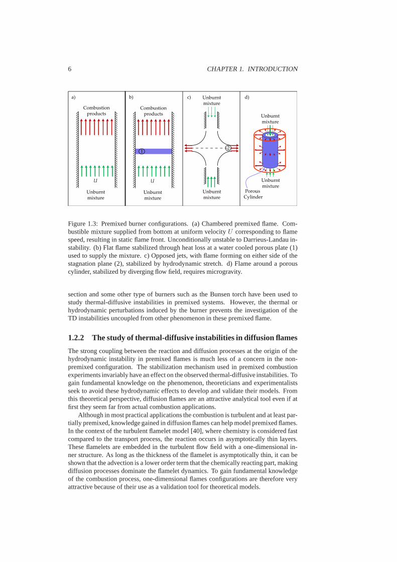
Because of the practical importance of this flame speed, the first experimentationson flat flames were aimed at determining the characteristic velocity of the propagationof a flame front in a combustible mixture. The pioneering workof Mallard and LeChatelier [30] on a simple laminar flame front traveling in a tube revealed the thermalnature of the mechanism responsible for flame propagation. For an interesting histor-ical perspective with illustration of the apparatus used, see the review of Oppenheim[31]. It was not until much later than Darrieus [32] and Landau [33] independentlydemonstrated that such planar deflagration fronts are inherently unstable. It is the muchstronger coupling between the reaction and diffusion processes [26, 28] in this config-uration that gives rise to aerodynamic instabilities resulting from thermal expansion.This Darrieus-Landau instability makes flat flame fronts simply established in a cham-bered flow of combustible mixture (figure 1.3(a)) unpractical for experiments aimedat investigating flame dynamics because of the strong coupling between this impor-tant hydrodynamic effect and the combustion process. Experimental results of a planarflame front deformed by the Darrieus-Landau instability is presented in [34]. A proce-dure allowing the creation of unstrained planar premixed flames is described by Searby[35]. It involves keeping the bulk velocity in the chamber offigure 1.3(a) at a criticalvelocity different that the laminar flame speed to avoid the Darrieus-Landau instability.More commonly, to study thermal-diffusive instabilities in premixed flames withoutthese complications, the hydrodynamic instability is usually stabilized either throughheat loss of hydrodynamic strain.
A premixed flat flames can be generated by supplying a combustible mixture througha porous injection plate because of the stabilizing effect of heat loss at the plate [36],see sketch in figure 1.3(b). However, this approach induces important perturbation ofthe flame front because of the heat loss and possible upstreamdiffusion of radicalstowards the cold injection plate, where they are neutralized through wall collisions.Another approach consists at opposing free jets of the combustible mixture, resultingin the formation of two planar flames on either sides of the stagnation plane formedby the jets impinging one another, see [37] for pictures and figure 1.3(c) for a concep-tual sketch. The radial expulsion of combustion products creates a velocity gradient,stretching and stabilizing the flame. This stretch has been shown to also have a strongeffect on thermal-diffusive instabilities [29] and extinction [37], making this config-uration of limited use to study these phenomena. Finally, ifthe combustible mixtureis injected through a porous cylinder, the flow rate can be adjusted so that the diverg-ing flow field stabilizes the flame [38], as shown in figure 1.3(d). However, buoyancyforces tend to break symmetry through the Rayleigh-Taylor instability [39] if the ex-periment is not carried out in microgravity.
One dimensional flame generated using the burner configurations mentioned in this
6 CHAPTER 1. INTRODUCTION
a) b) c) d)
U
Unburntmixture
Combustionproducts
U
Unburntmixture
Combustionproducts
1
Unburntmixture
Unburntmixture
2
Unburntmixture
Unburntmixture
Porous Cylinder
Figure 1.3: Premixed burner configurations. (a) Chambered premixed flame. Com-bustible mixture supplied from bottom at uniform velocityU corresponding to flamespeed, resulting in static flame front. Unconditionally unstable to Darrieus-Landau in-stability. (b) Flat flame stabilized through heat loss at a water cooled porous plate (1)used to supply the mixture. c) Opposed jets, with flame forming on either side of thestagnation plane (2), stabilized by hydrodynamic stretch.d) Flame around a porouscylinder, stabilized by diverging flow field, requires microgravity.
section and some other type of burners such as the Bunsen torch have been used tostudy thermal-diffusive instabilities in premixed systems. However, the thermal orhydrodynamic perturbations induced by the burner preventsthe investigation of theTD instabilities uncoupled from other phenomenon in these premixed flame.
1.2.2 The study of thermal-diffusive instabilities in diffusion flames
The strong coupling between the reaction and diffusion processes at the origin of thehydrodynamic instability in premixed flames is much less of aconcern in the non-premixed configuration. The stabilization mechanism used in premixed combustionexperiments invariably have an effect on the observed thermal-diffusive instabilities. Togain fundamental knowledge on the phenomenon, theoreticians and experimentalistsseek to avoid these hydrodynamic effects to develop and validate their models. Fromthis theoretical perspective, diffusion flames are an attractive analytical tool even if atfirst they seem far from actual combustion applications.
Although in most practical applications the combustion is turbulent and at least par-tially premixed, knowledge gained in diffusion flames can help model premixed flames.In the context of the turbulent flamelet model [40], where chemistry is considered fastcompared to the transport process, the reaction occurs in asymptotically thin layers.These flamelets are embedded in the turbulent flow field with a one-dimensional in-ner structure. As long as the thickness of the flamelet is asymptotically thin, it can beshown that the advection is a lower order term that the chemically reacting part, makingdiffusion processes dominate the flamelet dynamics. To gainfundamental knowledgeof the combustion process, one-dimensional flames configurations are therefore veryattractive because of their use as a validation tool for theoretical models.

1.3. OBJECTIVES AND SCOPE OF THE THESIS 7
Several configurations are available to generate diffusionflames for research pur-poses. As with premixed flames, the challenge resides in keeping the transport processsimple (ideally it should be strictly one-dimensional) andin avoiding thermal or hy-drodynamic perturbations, such as strain. A very simple one-dimensional diffusionflame configuration was introduced as theoretical constructfor research purposes byKirkby and Schmitz [41]. The combustion chamber is a straight duct open at oneend to a fast stream of oxidant and supplied at the other with fuel through a semi-permeable membrane. A sketch is provided in figure 1.4(a). All transport processesare one-dimensional with the oxidant counter-diffusing against the flow of products tothe planar reaction sheet. In such a simple configuration, analytical solutions can befound for the governing equations and numerous stability models have been developedusing this system [42, 43, 44, 45, 46, 47]. These models predict a planar stable flamesheet when far from extinction. Unfortunately, this burneris impossible to realize inpractice because of the perturbations induced by the fast stream required to removethe products and supply the oxidant above the chamber. Therefore, these theoreticalmodels remain without quantitative experimental validation.
The opposed jet flame presented in figure 1.4(b) has been used extensively to gen-erate flat diffusion flames. The strain induced in the flame as the products are forcedradially makes this configuration useful for the investigations on the effects of strain onthe chemistry [48, 49], extinction limits [50] and stability of diffusion flame [51]. Theunavoidable nature of this strain, its high magnitude and its stabilizing effect impliesthat this configuration is of limited use to study thermal-diffusive instabilities.
Low strain diffusion flame have been generated close to the forward stagnationpoint of porous cylinders and hemispherical caps [52], injected with fuel and placedin a slow stream of oxidant. A sketch is presented in figure 1.4c), for a review ofvarious counterflow diffusion flame configurations see [53].With great care, the strainrate can be kept as low as1.4 s�1 [52] by using a large radius porous injector. Usingthis type of burner, thermal-diffusive instabilities wereobserved close to the extinctionlimit showing qualitative agreement with numerical models[54]. The influence ofhydrodynamics is still important in this burner and prevents the formation of durableinstability patterns, making comparison with theoreticalmodels difficult.
A novel research burner configuration was recently introduced [55, 56] that allowsthe creation of flat one-dimensional nearly-unstrained diffusion flames. In this thesis,the original experiment is improved and a new symmetrical version is built. A sketchof the original configuration is presented in figure 1.4d). Indesigning this burner, greatcare was taken to reduce to a minimum all causes of flame stretch: aerodynamic strain-ing, flame curvature and flame/flow unsteadiness [57]. The resulting flame is ideallywell suited to study thermal-diffusive instabilities uncoupled from parasitic effects.The results gathered during this thesis and presented here will allow the first quantita-tive experimental validation of the theoretical models developed in the simplified one-dimensional counter-diffusing configuration of figure 1.4(a). Such comparison enablesthe identification of the critical simplifying assumptionsmade during the theoreticaldevelopments and their influence on the models precision.
1.3 Objectives and scope of the thesis
The main objective of this thesis is to further develop and characterize the novel quasi-unstrained one-dimensional counter-diffusion research burner recently introduced bythe Laboratory of Fluid Mechanics at the Swiss Federal Institute of Technology Lau-

8 CHAPTER 1. INTRODUCTION
a) b) c) d)
UFuel
Oxidizer Stream
Oxidizer
Fuel
FuelOxidizer Oxidant
Products Products
Fuel
U
Semi-permeablemembrane
Figure 1.4: Non-premixed burner configurations. (a) Idealized unstrained one-dimensional chambered flame model. (b) Opposed jet counter-diffusion configuration.(c) Low-strain hemispherical cap burner. (d) Novel quasi-unstrained counter diffusionburner, the design used and improved in this thesis.
sanne (EPFL-LMF) [55, 56]. Improvements are implement on the existing version(Mark I) and a new version is designed and constructed (Mark II). The new versionfeatures a symmetric design that allows control over bulk flow magnitude and directionacross the flame sheet. These unique experimental facilities are used to quantitativelyvalidate theoretical models of diffusion flame stability developed in the idealized one-dimensional configuration of figure 1.4a).
The comparison between experiment and theoretical models necessitates the im-plementation of specific measurement techniques. A necessary preliminary objectiveof the present work is therefore to select and implement measurement techniques suit-able to gather data useful for the validation of theoreticalmodels. Mass spectrometryis used in order to quantify the effective mixture composition supplied to the burnerand the species concentration profiles across the burning chamber.
The scope of the work presented here is the experimental investigation thermal-diffusive instabilities of unstrained diffusion flames. The unique experimental facilitiesdeveloped during this thesis offer vast possibilities for original research in the field ofcombustion. The present investigation will be limited to thermal-diffusive instabilitiesresulting in the formation of a cellular flame pattern or in planar intensity pulsations.
1.4 Contributions
Novel research burner configuration, description and characteriza-tion
Chapters 4 and 6: the recently introduced unstrained counter-diffusion burner has beenimproved and measurements have been carried out to verify that it is indeed a good ap-proximation of the idealized one-dimensional flame configuration. The working prin-ciples of the burner are described and the flame produced characterized as a function
1.5. THESIS OUTLINE 9
of the operating parameters.Work partially published in U.S. Combustion meeting, 2007 and International Sym-
posium on Combustion 2008. Accepted for publication in Proceedings of the Combus-tion Institute, vol. 32, 2009. Detailed configuration description and characterization tobe submitted to Combustion and Flame.
Mass spectrometer calibration procedure over a wide concentrationrange
Chapter 5: through the use of a semi-automated gas mixture generator and the devel-opment of a novel calibration procedure, an inexpensive mass spectrometer has beencalibrated to drastically improve its accuracy for the quantitative measurement of com-plex mixture composition over a wide concentration range.
Work to be submitted to Measurement Science and Technology.
Mapping of Lewis number parameter space and scaling of the insta-bilities
Chapter 7: the use of a two-inert dilution mixture allows themapping of extendedregions of the Lewis number parameter space for instabilities while keeping mixturestrength roughly constant. Using the same oxidant and fuel allowed the generationof the first experimental stability map of a diffusion flame inthe absence of any hy-drodynamic effects. The experimental measurements carried out in both cellular andpulsating flames describe the scaling of the instability properties as a function of thephysical parameters of the flame.
Work to be submitted to Combustion and Flame.
1.5 Thesis Outline
• Chapter 2 reviews the literature on theoretical, experimental and numerical in-vestigations of the instabilities of unstrained diffusionflames. The focus is onproviding the state of the art rather than giving technical details on the variousapproaches used.
• Chapter 3 deals with theoretical considerations relevantto the present investi-gation. The simplified one-dimensional counter-diffusionflame construct usedto develop theoretical models is presented. Since this thesis is principally ex-perimental in nature, the theoretical developments presented will be limited tothe minimum necessary to properly compare the models with the experimentalresults.
• Chapter 4 presents the experimental facilities used. The improvements imple-mented on the Mark I burner are presented. Design choices made for the MarkII version are explained and the construction process is described. The equip-ments used for mixture preparation, velocity and temperature measurement aredescribed.
• Chapter 5 covers the extensive developments that were madefor the calibrationof the mass spectrometer used. A novel calibration procedure is introduced to

10 CHAPTER 1. INTRODUCTION
account for the intrinsic non-linearities of this type of instrument over the widemixture concentration ranges encountered in this experiment.
• Chapter 6 covers the measurements that were made to characterize this newburner configuration and verify that it is indeed a good approximation of theidealized one-dimensional configuration.
• Chapter 7 presents the measurements that were made on the thermal-diffusiveinstabilities. The influence of the Lewis number is studied by diluting the reac-tants in a two-inerts mixture. A mapping of instabilities and extinction limits inthe Lewis number parameter space is shown. Finally, the cellsize and pulsationfrequency scaling in unstable flames is treated, as a function of both the Lewisnumbers and bulk velocity.
• Chapter 8 provides conclusions and future research perspectives opened by thenovel experimental facility presented here.

Chapter 2
State of the art
The subject of instability in combustion has generated an extensive and diversifiedliterature. The current presentation will be limited to thesubject of thermal-diffusiveinstabilities, with a clear emphasis on the non-premixed configurations. The interestedreaders are directed to the broader reviews of the field by Sivashinsky [26], Buckmaster[27], Clavin [28] and Matalon [29]. As the review articles presented above clearlyshow, research in the field of combustion instabilities has focused until recently onpremixed rather than diffusion flames.
This imbalance between the premixed and non-premixed configuration probably re-sides not it lack of interest but rather in the difficulty to observe thermal-diffusive insta-bilities in simple diffusion flames suitable for analyticaltreatments. Cellular structuresin premixed flames have been noticed a long time ago on Bunsen burners [58, 59] andlater recognized as part of the greater family of thermal diffusive-instabilities [60, 61].The ability to generate flat premixed flames in the controlledconditions of the lab-oratory using a uniform flow kept equal to the laminar flame speed then sparked theintensive research using this configuration mentioned in the review articles listed above.
The first experimental evidence of thermal-diffusive instabilities in a non-premixedflame came much later, with the work of Garside & Jackson [62].Since then, researchon the instabilities of diffusion flames has gained momentum. This is especially truefor in the past two decades, when the push to reduce emissionsmeant that combustionsystems tend to be operated with partially premixed lean mixtures, making them moreprone to develop this type of instability. This chapter is divided as follows, first theliterature is review for theoretical investigations will be presented, followed by theexperimental and finally a glimpse at the numerical approaches used will be shown.
2.1 Theoretical studies
Before Garside & Jackson [62] made their first documented observations of cellularinstabilities in diffusion flame, the non-premixed received some attention from theo-reticians. The term diffusion flame was introduced by Burke and Schumann [63] intheir landmark paper of 1928 in which they studied the flames formed between con-centric and co-flowing streams of fuel and oxidant. At the time, they did not report pre-vious theoretical investigation on the properties and shape of diffusion flames. Theydevised a simple theory, assuming constant velocity, equaldiffusion coefficients forthe two species and one-dimensional transport (radially).They also did not treat the
11

12 CHAPTER 2. STATE OF THE ART
chemical kinetics part of the problem and collapsed the reaction zone to an infinitelythin surface. Bypassing the internal structure of the reaction zone in the analysis greatlysimplified the problem. Using these assumption they achievegood agreement for flameshape between their theory and experimental flames formed using hydrogen, city gasor methane as the fuel and air as the oxidant.
Later, Zeldovich [64] performed a more complete investigation of the combustionof initially unmixed gases in a similar configuration. He added the assumption thatboth reactants molecular diffusivities are equal to the thermal diffusivity, resulting inboth Lewis numbers being equal to1. Using a burner configuration analogous to theone of Burke and Schumann [63], he obtained theoretical results for the species andtemperature distribution at the flame, showing that they were the same as for a preparedmixture in stoichiometric proportions. He also demonstrated that contrary to premixedflames where the reaction rate is determined by the physico-chemical properties ofthe reactants, in diffusion flames the reaction rate can be limited by the mixing ratebetween the reactants.
To study the unperturbed diffusion phenomena controlling the dynamics of thesenon-premixed flames, a one-dimensional theoretical construct was later introduced bySpalding at al. [65, 66]. It is a variation of this configuration that is created experi-mentally in the novel burner developed for this thesis. The theoretical model Spalding& Jain developed uses again the assumption of unity Lewis numbers, referred to asthe normal diffusion assumption(NDA), but considers temperature dependent trans-port properties and finite rate chemical kinetics. The maximum reaction rate wasdetermined and compared to an analogous premixed flame and the extinction limitswere found. The authors concluded that the maximum reactionrate can probablybe predicted by the Zeldovich-Spalding theory but point outthe lack of experimentalvalidation, especially regarding fuel leakage through theflame. This idealized one-dimensional flame configuration has been used extensively since then to develop in-creasingly complex theoretical models and will be described in detail in chapter 3.
The early models described previously used broad assumptions and were aimedat predicting basic flame parameters such as shape, reactionrate, temperature and ex-tinction. Subsequent models either pursued broader goals or grew in complexity, ac-counting for more variables and relaxing some assumption. Kirkby & Schmitz [41]were the first to tackle the task of studying theoretically the stability of the planardiffusion flames formed in the idealized one-dimensional configuration. They consid-ered the sensitivity of the model developed by Spalding & Jain [66] to infinitesimaldisturbances, using constant transport properties and allowed the Lewis number to bedifferent than unity. They found that the stability of the steady burning state to smallperturbations must be analyzed and demonstrated a reduction in the domain of possi-ble burning mixture caused by instabilities. More precisely, they identified temperatureoscillations in mixtures with Lewis number above unity as a possible mechanism forextinction. Kirkby & Schmitz [41] used numerical methods onthe model to obtainthese results. At the time, computing power was scarce and expensive, limiting theamount of parameters that could be investigated simultaneously. More modern numer-ical approaches to thermal-diffusive instabilities in combustion will be presented insection 2.3.
The introduction of activation energy asymptotic, notablythrough the work ofLi nan [67, 68], yielded results covering the entire range of Damkohler number, fromthe Burke-Schumann limit of infinitely fast chemistry down to extinction. The DamkohlernumberDa is the ratio of the characteristic residence time to the characteristic chem-ical time and is used extensively to characterize the intensity of the chemical reaction

2.1. THEORETICAL STUDIES 13
in a burning flame. Such analyzes yield the precise location of the reaction zone thatcan be treated as a thin reaction sheet. Plotting the maximumflame temperature as afunction of the Damkohler number yields the typical S-shaped response curve of theflame. Traveling along the curve with increasingDa, the flame condition jumps from afrozen-flow ignition regime to a near-equilibrium diffusion controlled regime where athin reaction zone sits between two regions of equilibrium flow. In between those twoextreme regimes, intermediate states with significant leakage of reactants through thereaction zone exist in which instabilities can occur. This leakage was demonstrated byLi nan to occur at lowDa in non-premixed flames, where the mixing rate can exceedthe reaction rate, implying that one or both reactants can pass through the flame frontwithout reacting completely. Response curves and their uses will be discussed furtherin section 3.2.1.
The use of large activation energy asymptotic allowed many parameters to be con-sidered simultaneously in theoretical models. One of the first such theoretical investi-gation to be applied to the idealized one-dimensional configuration is that of Matalon& Ludford [69] who obtained explicit response curves for thewhole range ofDa.Their asymptotic treatment of Kirkby and Schmitz’s problemincluded a wide rangeof parameters that were initially overlooked because of thehuge computing power re-quirements of the numerical method initially employed. Apart from the more completeresponse curves, their main results included explicit formulas for the extinction andignition points.
At the time, the theoretical models on laminar diffusion flames mentioned abovewere considered to be more or less without practical applications since in practice mostcombustion occurs in turbulent flows with fuel and oxidant atleast partially premixed.This view changed following the work of Peters [70] which views a turbulent diffusionflame as an ensemble of laminar diffusion flamelets. In this perspective, the counter-flow laminar diffusion flame used in the theoretical studies mentioned above becomesa representative configuration to investigate the behaviorthe laminar flamelets. Theseflamelets are then used to model the partially premixed turbulent combustion regimepresent in most practical applications. The flamelet model accounts for the fact thatin partially premixed turbulent flames, the local diffusiontime scales can vary con-siderably, locally loweringDa and breaking the fast chemistry assumption, leading tonon-equilibrium effects such as increased pollutants or soot formation.
Since then, numerous research groups have investigated thestability of diffusionflames using the planar flame produced in the simplified one-dimensional configura-tion as the base state. Among the most notable and active onesare those of Matalon[44, 71], Kim [42, 72] and Miklavcic [73, 74]. Each group useda slightly differenttheoretical burner configuration, set of boundary conditions, simplifying assumptionsand mathematical treatment, yielding different results. The crux of their approaches in-volves taking the Zeldovich numberΘ (the ratio of the activation energy to the thermalenergy, also called the activation-energy parameter) as a large perturbation parameterto perform activation-energy asymptotics. The detailed stability model formulation be-ing outside of the scope of this work, the interested reader is referred to the above listedpapers themselves for further details. Our work will be compared primarily to the mod-els developed by Matalon et al. [44, 71] because they includeeffect of a relatively largenumber of control parameters on the stability of an unstrained 1-D diffusion flame withfinite rate chemistry. For example, they allow for both Lewisnumbers to be differentthan one as well as unequal while the other models assume equal Lewis Numbers or a

14 CHAPTER 2. STATE OF THE ART
singleeffective1 Lewis number.Their results will be used extensively in this thesis which aims to provide the first
experimental results allowing validation of these models.Most of the works citedabove focused in identifying the regions on the S-Curves where instabilities can oc-cur and investigating the nature of these instabilities. The highlights of these papersis that as the Damkohler number is decreased, bringing the flame closer to extinction,instabilities can arise from the competing mechanisms of thermal and molecular diffu-sion. These instabilities can results in stripped quenching patterns (cellular flames) orintensity pulsations. The type of instability, if they occur at all before extinction, willdepend on the Lewis numbers of both the fuel (Lef ) and the oxidant (Leo) which aredefined as the ratio of thermal to molecular diffusivities.
All of these research groups generally predict cellular type instabilities for Lewisnumbers below 1 and intensity pulsation for Lewis numbers above 1, with slight vari-ations in critical Lewis numbers depending on other flame parameters such as mixturestrengthφ. According to the work using linear stability theory carried out by the Mat-alon group, the cell size is expected to scale with the diffusion lengthld, which isdefined asDth2U , divided by the critical wavenumber in the marginally stable state,σ� [44]. In a similar manner, the pulsation frequency is also expected to be well definedand scale withDth2U2 multiplied by the critical frequencyωI . Kukuck and Matalonpredicted that the pulsation frequency should be in the range of 1-6 Hz for typical ex-perimental flames [71]. A recent paper by Wang et al. [75] presents a detailed mappingof the pulsation instabilities, using bifurcation analysis based on the asymptotic ap-proach of Cheatham and Matalon. They predict that stable oscillations are possible ina restricted parameter range. These oscillations can either stabilize by themselves orgrow in amplitude and lead to flame extinction.
2.2 Experimental studies
Thermal-diffusive instabilities have been observed sincethe late 19th century in pre-mixed flames through the polyhedral structure they confer toBunsen flame in certainburning conditions[58, 59]. The first evidence that this type of instability can alsooccur in diffusion flames came up much later in 1951 and is attributed to Garside andJackson [62], who were originally investigating polyhedral flames structures in the pre-mixed configuration. They noticed that when the reactants are provided separately toan axi-symmetric jet burner, a polyhedral flame structure can be observed if the fuel,hydrogen in this case, is mixed with an inert gas. Since thesefirst chance observations,many experimental investigations have been aimed specifically at thermal-diffusive in-stabilities in diffusion flames.
Using a splitter plate burner, Dongworth and Melvin [76] also observed cellularpattern at the base of diffusion flames close to the lean extinction limit. They postulatedthat these instabilities were caused by fuel leaking through the base of the flame andforming a composite premixed/diffusion flame where instabilities could develop on thepremixed side. Later Ishizuka and Tsuji [77] observed striped quenching patterns indiffusion flames formed at the forward stagnation surface ofa porous cylinder. The fuelis inserted through the cylinder that is placed in a stream ofoxidant. Using hydrogen as
1Following this approach [72], the effective Lewis number isdetermined from the Lewis numbers of bothreactants weighted by the mixture strength. Information isloss in this process because the same effectiveLewis number can be produces from different combinations ofthe reactants Lewis numbers and result indifferent stability characteristics.

2.2. EXPERIMENTAL STUDIES 15
the fuel and air as the oxidant, they observed cells when the fuel was diluted in nitrogenor argon, but not when diluted in helium. They argued that thecells were caused bypreferential diffusion of H2 relative to O2. Cells occurred when the flame was locatedon the fuel side of the stagnation layer and were prevented when the flame moved tothe oxidant side.
A exhaustive review of the counterflow diffusion burner configurations availablefor research purposes was presented by Tsuji [53]. Some of these burners were illus-trated in figure 1.4. The burner types that are treated in thispaper are: the opposedjet flame, opposed matrix burner, flames located at the forward stagnation point ofa porous hemispherical cap, and flames located at the forwardstagnation point of aporous cylinder, also called the Tsuji burner. The author presents the characteristics ofeach burner but very little is said about the potential of each configurations for researchaimed at thermal-diffusive instabilities, save a mention of striped quenching pattern ob-served before extinction in the Tsuji burner with some reactant compositions. It shouldbe noted however, that all of these burner types induce a significant strain on the flame.Little has changed since then so far as burner configurationsare concerned, except afew improvements aimed at reducing the strain experienced by the flame. A notableimprovement is of course, the recent introduction of the burner configuration used inthis thesis.
With the rise in interest towards diffusion flames in the lasttwo decades, moresystematic experimental investigations on thermal-diffusive instabilities in this config-uration were realized. One of the first such study is that of Chen et al. [78], whoused a slot-jet (Wolfhard-Parker) burner with a wide variety of fuels and inerts to pro-duce cellular flames. The authors point out that the choice ofthe burner configurationwas guided by the flame strain in opposed jet flames inhibitingcellularity and axi-symmetric burners of the type used by Burke and Schumann exhibits curvature effectsthat also perturb the instabilities. Their results includemaps of where cells were en-countered as a function of the inert used, the oxidant concentration and the flow veloc-ity. They concluded that the non-premixed instabilities observed were similar in naturewith the cellular instabilities observed in premixed flames. They where observed closeto extinction when leakage and intermixing are expected to be significant across theflame front. The cellular instabilities are associated withconditions where the Lewisnumber of the more consumed reactant is sufficiently below unity, a threshold that theyestimated at aboutLe � 0.8.
In a recent paper by Han et al. [52], great efforts were taken to reduce as muchas possible the strain in a flame formed at the forward stagnation point of a poroushemispherical cap immersed in a stream of oxidant. To do so, asintered porous burnerof very large radius (5.22 m) and a very low speed oxidant stream were used. However,since the combustion products are still evacuated radially, the flame is strained. Themagnitude of the strain is evaluated on the order ofKs � 1.4s�1 in the center of theburner, but was not evaluated across the whole burner cross-section and the effect ofcurvature was not included. Using methane diluted in nitrogen, they observed holesand stripes in the flame sheet. The stripes they observed werealways aligned alongthe unstrained tangential direction and being advected radially outwards by the bulkflow of products. This indicates at least some aerodynamic effects on the instabilitiesthey generated since no static flame patterns where observed. The flame stability wasplotted as a function of the nitrogen dilution and the fuel injection speed, identifyingregions where cellular instabilities occur. However, no mention of the Lewis number ofthe reactants, their variations or their effect of the flame patterns observed were made.
Within the Laboratory of Fluid Mechanics (LMF) at the Swiss Federal Institute of

16 CHAPTER 2. STATE OF THE ART
Technology in Lausanne (EPFL) our research group has been active in experimentalinvestigations of thermal-diffusive instabilities in diffusion flames. Using methane andpropane flames, Furi et al. [79] observed thermal-diffusion induced pulsations in a axi-symmetric jet flame. These heavy fuels with oxygen diluted innitrogen allowed theLewis numbers to be above unity, enabling the onset of this type of instability closeto extinction. The occurrence of pulsation instabilities was mapped as a function ofthe jet velocity and the oxygen content of the oxidant stream. The observed pulsationfrequencies were in the order of a few Hz.
Cellular flames where also observed and investigated in the same axi-symmetric jetburner and in a two-dimensional slot burner (Wolfhard-Parker). Lo Jacono et al. [80]considered the effect of both reactants Lewis numbers and the initial mixture strengthon the cellular patterns found, in addition to the parameters considered in the paperspresented above. The regions where cellular flames formed close to extinction whereplotted in the Lewis numbers (of both reactants) parameter space and as a function ofboth reactants initial concentrations in the supplied streams. Using H2-O2 diluted inCO2, they found that when decreasing initial mixture strength,cells appeared over alarger portion of the parameter space. Depending on flow conditions, they observedbetween 1 and 6 cells on their 7.5 mm diameter burner. In the flames having between1 and 3 cells, the pattern was rotating.
In a subsequent paper using the same configuration, Lo Jaconoand Monkewitz [81]investigated the effect of numerous parameters on the cell size. These included burnergeometry, injection velocities, mixture strength and reactant transport properties. Theobserved cellular pattern was carefully mapped in the reactant concentration-jet ve-locity for both the axi-symmetric and slot burners. The scaling of the cell size wasreported as a function of the vorticity thickness of the mixing layer where the flame islocated and the Reynolds number based on the injection nozzle. A variation of the cellsize was also observed as a function of the mixture strengthφ, with the cells growingwith increasingφ.
Our group recently introduced of a novel research burner configuration [55] thatallows the creation of quasi-unstrained one-dimensional diffusion flames. This openednew research opportunities for the investigation of thermal-diffusive instabilities in dif-fusion flames in the absence on hydrodynamic effects. The first results in this newburner where published by LoJacono et al. [55, 56]. The results gathered coveredthe variation of the flame position as a function of mixture strength and a preliminarymapping of the instabilities as a function of the fuel and oxidant composition of thefeed streams. However, drawback in the first version of this new design were pointedout, namely that a residual strain remained, inducing cell motion and that the effectivemixture strength could not be determined a priori from the supplied reactants streams.Therefore, these results should be considered only qualitatively. One of the first tasksin the present thesis was modifying the experimental setup to allow quantitative mea-surements and comparison with theory.
2.3 Numerical methods
The recent advances in computer hardware that now provides colossal amounts of com-puting power at the disposal of research scientists has changed the way that numeri-cal methods can be used in the field of combustion. The numerical results of Kirkby& Schmitz [41] where of limited scope because of the limited amount of computingpower available at the time. Comparatively, the asymptoticmethods available shortly

2.3. NUMERICAL METHODS 17
after allowed for models to include more parameters and yield analytical results forimportant flame characteristics (i.e. ignition and extinction).
However, using asymptotic methods to find the dispersion relation used in the mod-eling of the instabilities, as in the last papers listed in section 2.1, still requires substan-tial numerical treatment because the dispersion relationsfound are transcendental. Thisexplains why many of the most recent work cited in section 2.1include substantial nu-merical results. Modern computer hardware allows the free-boundary problem to besolved directly using numerical methods, an approach that permits inclusion of moreparameters in the analysis that the asymptotic method, suchas density variations [82].Here will be presented a selection of recent numerical investigations on the stability ofdiffusion flame that will also benefit from the unique experimental results presented inthis thesis for validation.
Direct numerical simulation work on pulsating flames by Sohnet al. [83] haverevealed the occurrence of pulsations that can either decayof grow in amplitude andlead to flame extinction, depending on the Damkohler numberbefore the perturbation.The authors suggested that the threshold Damkohler number, below which the flamecannot recover stability, could be used as a revised extinction criterion for diffusionflamelet library in the laminar flamelet regime of turbulent combustion. However, thisanalysis assumes that both Lewis numbers are equal and only alimited range of Lewisnumbers has been investigated.
In a numerical simulation including the effect of more parameters, such as a vari-able density, Christiansen et al. [84] investigated thermal-diffusive oscillations in hy-drogen and methane flames. They concluded that while all oscillations would ulti-mately lead to extinction, in certain flames this process could be slow enough to allowexperimental observation. They also argued that oscillations in hydrogen flames wouldbe too low in amplitude (5K) and too high in frequency (60 Hz) to be observed exper-imentally.
In the numerical study of cellular instabilities, striped patterns have been observedfor Damkohler numbers slightly above extinction. Lee and Kim [85] reported thatafter the emergence of the cellular pattern, a further decrease in the damkoler numberresults in a reduction of the number of cells observed on a two-dimensional opposedjet burner. Recently, Valar et al. [86] performed numerical simulations on the cellularpattern developing in axi-symmetric jet flames and reportedgood agreement with theexperimental results of Lo Jacono et al. [80, 56]. However, no recent numerical resultshave been found that address cellular flames in the idealizedone-dimensional diffusionflame that is the focus of this work.
The results obtained by Metzener and Matalon [45] will be used extensively inthis work because their model is the most complete we have encountered and wasdeveloped for a burner configuration compatible with our experimental realization. Itaccounts for the effects of many parameters and covering regimes of both cellular andpulsating flames. Parameters considered includes both Lewis numbers, which can bedistinct and different than 1, the initial mixture strengthand the flow conditions. Theinstability map presented in figure 2.1 is reproduced from their work and shows thepredicted regions where different types of instabilities are expected close to extinction,as a function of both Lewis numbers. The flame parameters for which this map wasgenerated can be reproduced in our experimental burner and the results presented inthis thesis will be compared to this numerical model. The same reference also providesother maps and general trends for different mixture strength and flow conditions, thevalidity of which can also be tested using our experimental methodology.

18 CHAPTER 2. STATE OF THE ART
���������¢ ���������������
��� �����������������¢
����������¢ � � ���
��Figure 2.1: Detailed map of the instabilities expected close to extinction as a functionof the Lewis numbers of both reactants, with an initial mixture strength ofφ � 0.5.Reproduced from reference [45].

Chapter 3
Theoretical considerations
In this chapter will be presented the fundamentals of the theoretical developments usedin the models that this experimental study aims to validate.The details of the linear sta-bility analysis are outside of the scope of this work and the interested reader is referredto the literature review of section 2.1 for a list of papers that covers this topic. Thefirst section will present a simple model for the stable flame generated in the idealizedone-dimensional counter-diffusion burner. The simplifying assumptions made will belisted and the main steps of the development explained. The results of interest are thetheoretical species and temperature profiles as well as the relation for flame position.These will be used later to assess how well our experimental realization approaches theidealized theoretical construct.
The only aspect of stability theory that will be presented here is the response curveof the flame, which links the flame burning rate to the Damkohler number. This charac-teristic S-shaped curve is very useful to illustrate the mechanisms that lead to the onsetof instability and flame extinction. Finally, numerical modeling was also employedin this thesis to provide stable flame structure data beyond the drastic simplifying as-sumption of the theoretical modeling. The strategy used wasbased on the Cantreasoftware package and will be detailed in the last section of this chapter. This tool wasalso used to determine the mixture transport properties from the measured compositionand temperature data.
3.1 Simple one-dimensional model forthe baseline flame
We start from the simplified theoretical model for the idealized chambered diffusionflame of figure 3.1(a) (see e.g. Cheatham & Matalon [44]). In the original configura-tion, one reactant (usually the fuel) is supplied from the bottom with a uniform velocityU , while the oxidizer is introduced from the top and reaches the reaction area solelyby diffusion against the flow of products. The distribution of oxidizer and products is‘magically’ kept uniform over the cross section by the fast top stream which removescombustion products and supplies reactant. In the following, this model is adapted tothe more general symmetric configuration shown in figure 3.1(b) with arbitrary bulkflow magnitude and direction imposed.
19

20 CHAPTER 3. THEORETICAL CONSIDERATIONS
UFuel
Oxidizer Stream
x = xf
Semi-permeablemembrane
Xo,0
Xf,L
Oxidizer Stream
Xo,0
Xf,L
Fuel Stream
x = L
U
a) b)
x = 0
Figure 3.1: a) Conventional chambered diffusion flame. b) Symmetric chambered dif-fusion flame with reversible bulk flow.
3.1.1 Reaction-sheet approximation
In the symmetric configuration, the fuel and oxidant are introduced uniformly over theburner cross section atx � 0 andx � L, respectively. In the following, dimensionalvariables and unscaled mass fractionsX are designated by. It is assumed that bothreactants follow Fick’s law of mass diffusion and burn in a global one-step irreversiblereaction 3.1.
νf fuel� νx oxidizerÈ� products�Q (3.1)
Next, we make the assumption of constant mass fluxρU and transport propertiesDi, κ and Cp, independent of temperature. In addition, it is reasonableto assumethat both reactants and the combustion products have identical mean molecular weightW , thermal diffusivityDth and specific heatCp since both reactants are diluted withan inert (CO2 in this case) that constitutes the bulk of the mixture. The steady-statedimensional equations of conservation of species are:
ρU∂Xo
∂x�Doρ
∂2Xo
∂x2� �νoWoω (3.2)
ρU∂Xf
∂x�Df ρ
∂2Xf
∂x2� �νfWf ω (3.3)

3.1. SIMPLE ONE-DIMENSIONAL MODEL FOR THE BASELINE FLAME 21
ρCpU∂T
∂x� λ
∂2T
∂x2� Qω (3.4)
Hereω is the chemical reaction rate,ρ the density of the mixture andWf ,Wo themolecular weights of the fuel and oxidant, respectively. The system is made dimen-sionless using the chamber lengthL as characteristic length andDth2L as characteristicvelocity. The reference temperature isq2Cp whereq � QXf,L2νfWf represents theheat released per unit mass of fuel consumed. The mass fractions of fuel and oxidizer,finally are scaled with the conditions where they are introduced: the fuel mass fractionby Xf,0 at x � 0 and the oxidizer mass fraction byφXo,L at x � L, whereφ is thefuel-to-oxidizer equivalence ratio.
φ � Xf,L2νfWf
Xo,02νoWo
(3.5)
Invoking the large activation energy approximation, whereit is assumed that noreaction occurs outside of a thin reaction sheet located atx � xf , the dimensionlessequations are obtained as
U∂Xo
∂x� Le�1o
∂2Xo
∂x2� �ωδ<x � xf A (3.6)
U∂Xf
∂x� Le�1f
∂2Xf
∂x2� �ωδ<x � xf A (3.7)
U∂T
∂x� ∂2T
∂x2� ωδ<x � xf A (3.8)
whereωδ<x�xf A � νfWfL2ω<xA�DthρXf,0��1. Here are introduced the Lewis num-bers for the fuelLef and the oxidantLeo, which are the rations of the thermal to themolecular diffusivities.
Lef � Dth
Df(3.9)
Le0 � Dth
D0
with Dth the thermal diffusivity andDf , Do the molecular diffusivities of the fueland oxidant, respectively. The Lewis numbers of both reactants will play a criticalrole in determining which type of instability, if any, can grow in the flame. The non-dimensional boundary conditions at the location of fuel andoxidizer injection atx � 0
andx � 1, respectively are
x � 0 � Xf � 1, Xo � 0, T � T0 (3.10)
x � 1 � Xo � φ�1, Xf � 0, T � TL (3.11)
To link the solutions across the flame sheet atx � xf , equations (3.6) - (3.8) areintegrated fromx � xf � 0 to x � xf � 0 to yield the jump conditions

22 CHAPTER 3. THEORETICAL CONSIDERATIONS
��T �� � ��Xo�� � ��Xf �� � 0 (3.12)��∂T
∂x� Le�1o
∂Xo
∂x ���∂T
∂x� Le�1f
∂Xf
∂x � 0 (3.13)
where the operator����� represents the jump of the respective quantity across the reactionsheet (the difference between its value atxf � 0 andxf � 0). These jump relations(3.12) and (3.13) represent respectively continuity of allvariables and the fact that thereactants have to reach the flame sheet in stoichiometric proportions to have completecombustion, i.e. to satisfy the boundary conditionsXo<x � 0A � 0 andXf <x � 1A � 0.
3.1.2 Model results
The above model corresponds to the leading order of the activation energy expansionof Cheatham [44], with slightly different boundary conditions resulting from the finitechamber length, and represents a stable planar flame sheet. Solving equations (3.6) -(3.8) in each sub-domain0 2 x 2 xf andxf 2 x 2 1 and applying the boundaryand jump conditions (3.10) - (3.13) yields the flame positionxf given by equation(3.14) and the exponential species and concentration profiles (3.15) - (3.17), whereTf is the adiabatic flame temperature defined by the jump relation. The theoreticalprofiles obtained from this simplified theory applied to a stable lean flame (φ � 0.5)are presented in figure 3.2.
e�ULef xf � 1
eULeo<1�xf A � 1� �φ (3.14)
Xo � bhhfhhd0 for 0 2 x 2 xf
1φ
eULeox�eULeoxf
eULeo�eULeoxf
for xf 2 x 2 1(3.15)
Xf � bhhfhhd eULef x�e
ULef xf
1�eULef xf
for 0 2 x 2 xf
0 for xf 2 x 2 1(3.16)
T � bhhhfhhhd <Tf�T0AeUx�T0eUxf �Tf
eUxf �1 for 0 2 x 2 xf<Tf�TLAeUx�TLe
Uxf �Tf eU
eUxf �eU
for xf 2 x 2 1(3.17)
It is interesting to notice in equation 3.14 that the flame position in the presentfinite length burner depends on the Lewis number ofboth species, in contrast to thesemi-infinite configuration of Cheatham and Matalon [44] where xf depends only onthe Lewis number of the species which has to diffuse against the bulk flow. In ourburner, when the bulk velocity is very small, both Lewis numbers become relevant forthe determination of flame position since for both species diffusion plays an importantin transport towards the flame.
When the bulk velocity is high, equation 3.14 agrees with theexpression given byCheatham and Matalon [44] as one would expect. In the limiting case of vanishingbulk flow U � 0, the expressions (3.14) - (3.17) have to be evaluated with Hˆopital’srule to yield the limiting flame position:

3.1. SIMPLE ONE-DIMENSIONAL MODEL FOR THE BASELINE FLAME 23
0
0.5
1
1.5
2
0 0.2 0.4 0.6 0.8 1 0
500
1000
1500
2000M
ass
Fra
ctio
n [ ]
Tem
pera
ture
[K]
Dimensionless position [ ]
U
0
0.5
1
1.5
2
0 0.2 0.4 0.6 0.8 1 0
500
1000
1500
2000M
ass
Fra
ctio
n [ ]
Tem
pera
ture
[K]
Dimensionless position [ ]
U
0
0.5
1
1.5
2
0 0.2 0.4 0.6 0.8 1 0
500
1000
1500
2000M
ass
Fra
ctio
n [ ]
Tem
pera
ture
[K]
Dimensionless position [ ]
U
Figure 3.2: Theoretical species concentration profiles (fuel � � �, oxidant� � �) andtemperature (—) profiles obtained from the simplified one-dimensional model. Theresults shown are for a CO2-diluted H2-O2 lean flame (φ � 0.5) with a bulk flow of 20mm/s.
xf <U � 0A � φLeo
φLeo � Lef(3.18)
In this limit of a purely diffusive flame without bulk flow, thetemperature andspecies concentration profiles become linear and will not beshown here.
3.1.3 Adiabatic flame temperature
In premixed flames, the calculation of the adiabatic flame temperature is a relativelystraightforward process. Assuming a complete depletion ofthe fuel, one simply has todetermine the amount of heat released and find the resulting temperature increase forthe unburned species and the products. In the diffusion flameconfiguration used here,the situation is complicated by the fact that the amount of the counter-diffusing reactantthat removes heat from the reaction zone is unknown. Considering the particular case ofcomplete combustion with the oxidant counter-diffusing, simply taking into account theamount of oxidant consumed results in a large overestimation of the flame temperature.
In the theoretical treatments of the problem found in the literature, the adiabaticflame temperature is often determined using a relationship (dimensionless) of the formgiven in equation 3.19 [44]. This equation is valid for the case where the oxidant isthe counter-diffusing species. The parameters used areT��, the temperature at theadvected end of the chamber,∆T the difference between the two supply temperatures,φ the mixture strength andLeo the Lewis number of the counter-diffusing species.However, since this approach assumes constant transport properties, it results in a con-siderable underestimation of the flame temperature when compared to the experimentalresults available.
Ta � 1 � T�� � <∆T � 1A<1 � φ�1A�12Leo (3.19)
In this thesis, the adiabatic flame temperature was determined considering that theheat released by the combustion is used to raise the temperature of three species. The

24 CHAPTER 3. THEORETICAL CONSIDERATIONS
first two are the inerts contained in the advected stream and the products of combustion.These are assumed to be raised to the flame temperature. The third contribution tothe heat expenditure includes part of the supplied counter-diffusing species that neverreaches the flame but is nonetheless heated above its supplied temperature. The choiceof the temperature at which this last contribution is raisedis somewhat arbitrary andhas a huge influence on the resulting adiabatic flame temperature. The assumptionused here is simply that the whole of the oxygen present at thecounter-diffusing endof the burner is raised to a temperature halfway between the injection temperature andthe flame temperature. This choices yielded results in very good agreement with theexperimental results and the values obtained from the numerical models presented insection 3.3.
3.2 Stability considerations
Theoretical investigation of the stability of diffusion flames usually involves applyingasymptotic methods to a simplified model similar to the one presented in the previoussection. The linear stability analysis is often performed by introducing a small per-turbing parameter in the stable base state [72, 44]. In thesestudies, it is customary toassume constant density to remove hydrodynamic effects from the analysis. The result-ing dispersion relation reveals the nature and flame conditions under which instabilitiescan develop in unstrained diffusion flames. Important parameters that must be includedin the analysis include both reactants Lewis numbers, the initial mixture strengthφ, thetemperature difference between the two ends of the chamber and the Damkohler num-ber. This critical parameter can be used to characterize theburning state of a flameusing the response curve concept that will be presented in section 3.2.1.
In the present thesis, the results of the group lead by Moshe Matalon will be usedextensively because they include the effect of more controlparameters [44, 71, 45]. Ofspecial significance is the inclusion of both reactants Lewis numbers, which are allowedto be different from each other and different from unity. Other linear stability analysisoften uses a singleeffective Lewis numberwhich is derived from both reactants Lewisnumbers weighted by the mixture strength [87, 73]. This operation, while simplifyingthe mathematics of the analysis, loses the information about the physical role of eachreactant in the onset of the instabilities.
In the limit of infinitely fast chemistry, the Burke-Schumann limit, there is not leak-age of reactants across the flame sheet and there is no real solutions to the dispersionrelation with a positive growth rate, the flame is unconditionally stable. In the case ofequal diffusion coefficients, whereLef � Leo � 1, the dispersion relation again admitsno real positive growths rates and the flat flame is again unconditionally stable [44].For all other cases of unequal diffusivities and finite-ratechemistry, instabilities canarise.
3.2.1 The response curve
A response curve relates the flame maximum burning temperature or reaction rate tosome flame parameter such as the reactants initial temperature, bulk flow velocity, etc.It is used to visualize certain states of the flame, ignition,stable burning solution, in-stabilities or extinction. In this section, the response curve linking the flame reactionrate to the Damkohler number will be used to illustrate the parameters involved in theonset of instabilities close to the lean extinction limit ofdiffusion flames.

3.2. STABILITY CONSIDERATIONS 25
The Damkohler numberDa is defined as the ratio of the residence time in thereaction zone to the chemical reaction time. The formulation of the Damkohler numbercan vary depending on the context it is intended to be used in.The form presented inequation 3.20 is applicable to the one-dimensional configuration used here and is takenfrom reference [44]. It covers the range of Damkohler numbers from an infinitelyfast rate of burning, the Burke-Schumann limit at the high end, down to instabilitiesand extinction at the low end. This range is sufficient here since our interest is in theonset of instabilities from an initially stable flame and notwith phenomena involvingignition. Da � λ
ρacpU2�R0Ta
EE3
νxcpW
qR0WfPBXf,�� exp<�E2RTaA (3.20)
Response curves for diffusion flames are typically S-shapeswith the three branchesrepresenting different burning regimes. They were first studied by Fendell [88] andLi nan [67], for a more recent and broader presentation, see [46]. A typical S-shapedresponse curve is shown in figure 3.3. On the bottom branch of the curve, the flowis nearly frozen, with a very small reaction rate. As the Damkohler number increasesprogressively, so does the reaction rate untilDa reaches a critical valueDa,I corre-sponding to ignition. The reaction rate then increases in aninfinite manner and theburning state jumps on the upper branch of the curve corresponding to intense burningrates. IfDa is further increased, the system approaches the Burke-Schumann limit ofinfinitely fast and complete combustion. On the other hand, if Da is decreased the re-action rate will follow the top branch and decrease slowly until another critical valueis reached,Da,E corresponding to extinction. The system state then jumps back on thelower branch of the curve with nearly frozen flow. The centralpart of the curve cor-responds to unstable states with a reaction rate decreasingwith increasingDa that cantherefore be considered physically unrealistic [46]. The portion of the top branch ofthe S-curve immediately before extinction is where the thermal-diffusive instabilitiesare predicted and observed.
In figure 3.4 is presented a close-up of the portion of the top branch of the S-Curve immediately adjacent to the extinction point. The solid red line represents stableburning states and towards the right, asDa is increased towards the Burke-Schumannlimit, the flame temperature tends asymptotically to the adiabatic flame temperature.The dashed line represents unstable burning states with thetransition point located atDa � D�
a being a marginally stable state. It is between this criticalvalueD�a and
extinction that the thermal-diffusive instabilities can develop and therefore it is therethat the experiments should be conducted.
In our experiment, we would like to be able to move downward onthe top branchof the S-curve to reach the unstable regime located immediately before extinction. Theways available experimentally to change the Damkohler number are limited and involvealtering the characteristic flow time or the characteristicreaction time. The latter canbe used to lowerDa by reducing the flame temperature, either through increasing thereactants dilution while maintaining their proportions constant or simply by changingthe mixture strength. Changing the dilution without changing the mixture strengthφ is difficult because of the inherent complexity of our experimental configuration.In practice, it is difficult to predict the effective boundary condition on the counter-diffusive injection side resulting from a change in dilution level, as will be explained insection 4.1. Therefore, the most convenient way to decreasethe Damkohler number inour experimental realization is to reduce the mixture strength by decreasing the amount

26 CHAPTER 3. THEORETICAL CONSIDERATIONS
Fla
me
tem
per
atu
re
or
bu
rnin
g r
ate
Damköhler number
Intensly burning branch
Weakly burning branch
Da,E Da,I
Ignition Point, I
ExtinctionPoint, E
Burke-SchumannlimitThermal-diffusive
instabilities
Figure 3.3: Typical S-shaped response curve linking the flame maximum burning tem-perature to the Damkohler number of the system. The square shaded region wherethermal-diffusive instabilities are observed is enlargedin figure 3.4.
Fla
me
tem
per
atu
re
or
bu
rnin
g r
ate
Damköhler numberDa,E Da*
Marginally stablestate
ExtinctionPoint, E
Burke-Schumannlimit
Ta
T*
TE
Figure 3.4: Enlargement of the S-curve region close to the extinction limit. The solidline represents stable burning states on the upper branch ofthe S-curve of figure 3.3.On the dashed line, between the marginally stable stateD�
a and extinction, are locatedthe unstable stated where thermal-diffusive instabilities can grow.
of fuel supplied in the fuel stream.It is also possible and easy to change the residence time by changing the bulk flow.
However, the range of experimentally achievable bulk flow islimited, ranging fromvery small values to about 30 mm/s. From the expression givenin equation 3.20 we

3.2. STABILITY CONSIDERATIONS 27
see thatDa varies as the inverse of the square of the bulk velocity and with the thirdpower of the adiabatic flame temperatureTa. The inability to significantly increase thebulk velocity to reach the lowDa where the instabilities are observed means that theflames are usually brought to instabilities simply by lowering the mixture strength todecrease the heat release, increasing the chemical reaction time.
3.2.2 Thermal-diffusive instabilities
The thermal-diffusive instabilities that can develop close to extinction in diffusionflames can take many forms, the distribution of which in the parameter space has beenthe subject many of the works reviewed in section 2.1. Of interest here are the instabil-ities that can be observed in the laboratory: mainly cellular flames and planar intensitypulsations. Other instability regimes are also expected from theoretical modeling, suchas oscillatory cells at the transition between the two modes. The concept of a thermal-diffusive instability evolving on very fast timescales, comparable to the characteristicchemical time was also demonstrated by Buckmaster et al. [89].
The driving mechanism behind these thermal-diffusive instabilities is the differen-tial diffusion between species and heat, both of which beingnecessary to sustain thecombustion reaction. The ratios of these quantities, the Lewis numbers introduced ear-lier in equation 3.10, are the key parameters that will determine what type, if any, ofinstability that will develop as the Damkohler number is decreased to approach extinc-tion. Naturally, if all diffusivities are equal, the flame isunconditionally stable to TDinstabilities. However if they are not, there will be eitheran excess or deficiency inavailable enthalpy in the reaction zone.
The sketch presented in figure 3.5 show qualitatively the location of the regionsof cells and pulsations expected in the Lewis number space. The figure is adaptedfrom reference [29], with pictures obtained in this work inserted in the regions of cellsand pulsations. The solid line represents the conditions where there is no excess ordeficiency of available enthalpyhf in the reaction zone. Above this line, there is adeficiency of enthalpy while below the line there is an excessof enthalpy. The verticaldashed line represents the effective mixture strength at the flameγ, with lean conditionshaving a negativeγ on the left and the rich conditions on the right.
Generally speaking, when the Lewis numbers are below unity,the thermal diffu-sivity is smaller than the molecular diffusivity and since all the heat cannot be carriedaway, there is an excess of available enthalpy in the reaction zone. This situation favorsthe creation of a cellular flame pattern at lowDa. The opposite situation where Lewisnumbers above unity yields a deficiency of enthalpy close to the flame results in pla-nar intensity pulsations. When considering the initial mixture strength, cells are morelikely to occur in lean flames and pulsations in rich flames [45]. The high-frequency in-stability regions shown in figure 3.5 corresponds to the fast-time instability introducedby Buckmaster et al. [89] and intervenes on such small time and length scales that theyare not expected to be observable in practice.
Stationary cellular flames are found when the fastest growing mode has a finitewavenumber and pulsation when this wavenumber is zero. In between those twodomains, the two types of instabilities can co-exist, resulting in oscillatory cellularflames. Theoretical studies [44, 71] reveal that the typicalsize of the cellular patternsis expected to scale with the diffusion lengthlD � Dth2ρcpU divided by the criticalwavenumber in the marginally stable state. In a similar fashion, the pulsation frequencyshould also be well defined and scale withDth2U2 multiplied by the critical frequencyin the marginally stable state.

28 CHAPTER 3. THEORETICAL CONSIDERATIONS
��
����� ���������
����������¢ �������������������¢�����
G����
��� �������������������¢
���������¢ ������������
����������¢ �� ������
Figure 3.5: Qualitative sketch of the types of instabilities expected close to extinctionas a function of the Lewis number of both reactants. This figure was adapted from ref-erence [29]. The inserted pictures illustrated the cellular flames that will be discussedin chapter 7.3 and the planar intensity pulsations that willbe discussed in chapter 7.4.
The locations of the various regions illustrated in figure 3.5 depends strongly on theflame parameters, especially the mixture strength. In a richflame the graph is stretchedalong the vertical axis and compressed on the horizontal axis with lean configurationshaving the opposite effects. If the roles of the two reactants are inverted, with the fuelnow having to counter-diffuse to the reaction zone, a similar map could be drawn. Inthis reversed configurations, the same regions would be found but their location wouldhave to be flipped relative to a line passing throughLeo � Lef .
3.3 Numerical tools
In this thesis, numerical tools were used to perform three tasks. First, to evaluate trans-port and thermodynamic properties for the complex gas mixtures encountered in thisexperiment. Second, to gather needed flame parameters, suchas the maximum flametemperature without having to perform lengthy experimentsfor every flame configu-rations used. Finally, to calculate species and temperature profiles beyond the drasticassumptions of the theoretical model, allowing comparisonwith the experiment. TheCantera software package [90, 91] was used for all of these tasks. Cantera is an open-source (distributed under the BSD software license), extensible software suite createdand maintained by D. G. Goodwin of Caltech. For the results presented here, Canterawas used only from within the Matlab environment.
The transport properties were evaluated using the NASA thermodynamic databasefor gas phase mixtures [92, 93]. Matlab code was written to interact with Cantera,

3.3. NUMERICAL TOOLS 29
either through a command line or a GUI interface. From the supplied mixture compo-sition and temperature data measured experimentally, the program returned the relevantmixture properties. Since at least one end of our burner is open to the atmosphere andthe pressure drop in the exhaust path is very small, the pressure in the burning chamberwas always assumed to be one atmosphere.
For all results presented here, the mixture composition at both ends of the burnerwas always measured or known from the prescribed gas stream.However, measuringthe composition and temperature in the reaction zone itselfwhere they are the mostrelevant to the analysis is difficult, lengthy and induces perturbations on the flame.Moreover, the mass spectrometry instrumentation implemented here to measure thecomposition in the chamber can only account for stable species. In the reaction zonewhere radicals are abundant, this can induce errors in excess of 10% [94].
When the mixture composition at the flame or the temperature data was not orcould not be measured experimentally, these values were evaluated from a numericalmodel of the burner. Supplying the measured boundary conditions to this model andsolving using the routines built into the Cantera package yielded the desired informa-tion about the conditions prevailing at the flame front. The reaction mechanisms usedin this model for both the methane and hydrogen flames encountered in this thesis wasGRI/Mech 3.0 [95]. This mechanism includes 53 species and 325 reactions. Althoughoptimized to model methane combustion, this mechanism is also widely used for hy-drogen combustion [95].
The use of numerical tools also allows to go beyond the assumptions used to de-velop the simple one-dimensional model for the baseline flame presented in section3.1. Using the same numerical model provided results on flameposition, species andtemperature profiles that can be compared to both the simplified model and the exper-imental data. Numerical results are presented in figure 3.6 for the same stable flamethat was used to generate the theoretical profiles of figure 3.2, which are also shownfor comparison purposed.
0
0.5
1
1.5
2
0 0.2 0.4 0.6 0.8 1 0
500
1000
1500
2000
Mas
s F
ract
ion
[ ]
Tem
pera
ture
[K]
Dimensionless position [ ]
U
0
0.5
1
1.5
2
0 0.2 0.4 0.6 0.8 1 0
500
1000
1500
2000
Mas
s F
ract
ion
[ ]
Tem
pera
ture
[K]
Dimensionless position [ ]
U
0
0.5
1
1.5
2
0 0.2 0.4 0.6 0.8 1 0
500
1000
1500
2000
Mas
s F
ract
ion
[ ]
Tem
pera
ture
[K]
Dimensionless position [ ]
U
0
0.5
1
1.5
2
0 0.2 0.4 0.6 0.8 1 0
500
1000
1500
2000
Mas
s F
ract
ion
[ ]
Tem
pera
ture
[K]
Dimensionless position [ ]
U
0
0.5
1
1.5
2
0 0.2 0.4 0.6 0.8 1 0
500
1000
1500
2000
Mas
s F
ract
ion
[ ]
Tem
pera
ture
[K]
Dimensionless position [ ]
U
0
0.5
1
1.5
2
0 0.2 0.4 0.6 0.8 1 0
500
1000
1500
2000
Mas
s F
ract
ion
[ ]
Tem
pera
ture
[K]
Dimensionless position [ ]
U
Figure 3.6: Species concentration (fuel– – –, oxidant- - -) and temperature (—) profilesobtained using the Cantera software package. The theoretical profiles from figure 3.2are shown with the black lines. The results shown are for a CO2-diluted H2-O2 leanflame ( phi=0.5 ) with a bulk flow of 20 mm/s.
The main differences between the two datasets is seen in the concentration profile

30 CHAPTER 3. THEORETICAL CONSIDERATIONS
of the advected species and in the location of the flame front.These discrepancies areexpected since in the theoretical model constant transportproperties are assumed andevaluated at the flame conditions. The advected species being supplied at a temperaturesignificantly lower that the flame temperature it is normal tosee a poor accuracy of thetheoretical model in this region. There is also a slight difference between the theoreticaland numerical models regarding flame position. Again, this difference can be explainedby a drastic assumption made in the simplified theory. By assuming that the chemistryis infinitely fast, the reaction zone collapses to an infinitely thin surface, which is notthe case in reality or in the numerical model which accounts for finite-rate chemistryand results in a finite thickness flame sheet.

Chapter 4
Experimental facilities andmethods
At the core of this thesis is the gathering of experimental data on the thermal-diffusiveinstabilities of diffusion flames in the absence of strain. In this chapter will be pre-sented the experimental facilities and techniques that were used for this purpose. Inthe first section will be described the two burners featuringthe novel species injectionarrays that allow the creation of the sought after unstrained flames. A more lengthydescription will be given for the second, or Mark II, versionof the burner since it wasbuilt specifically for this thesis.
Subsequent sections will cover the experimental means thatwere implemented toprobe the flame and measure its characteristic. First will bediscussed the photographicand cinematographic techniques used to record flame shape and motion. Then the waythe velocity and temperature profiles were measured will be presented. The last sectionwill cover the mixture generation setup. An extensive suiteof mass spectrometrictechniques were also developed specifically for this thesisand because of its extent,this topic will be treated separately in the next chapter.
4.1 The burners
The main challenge when attempting to create an unstrained chambered flame is tosupply the reactants and remove the products evenly across the reaction area. A novelway to address this problem and produce a truly unstrained flame has recently intro-duced at EPFL by Prof. Peter Monkewitz and successfully implemented [55, 96]. Inthis novel burner configuration, this difficulty is overcomeby supplying the reactantthrough an array of closely spaced needles while allowing the products to escape be-tween them. The result is a flame with very little residual strain which results mainlyfrom temperature inhomogeneities in the supply and exhaustpaths. This strain can beminimized and the supply configuration poses no restrictionfor the strain to be com-pletely eliminated, contrary to burners where the productsare evacuated radially. Thisunique configuration is ideally well suited to provide experimental validation for the-oretical diffusion flame stability models and accordingly has been developed in closecollaboration with Prof. Moshe Matalon who heads a very active research group work-ing on the theoretical side of the problem.
31

32 CHAPTER 4. EXPERIMENTAL FACILITIES AND METHODS
Oxidant
Products Products
Fuel
U
2
3
1
Figure 4.1: Schematic of the Mark I version of the burner. (1)The in injection array,(2) the injection layer and (3) the secondary burners.
4.1.1 Mark I burner
The first (Mark I) version of the burner was built by David Lo Jacono under the super-vision of Peter Monkewitz, starting in 2003. The first results gathered in this uniqueburner were published in 2005 [55, 56]. No results generatedin this thesis were gath-ered using this first iteration of the burner design as it was used for the publicationslisted above. The first results presented in this thesis and published in reference [96]were achieved using an improved version of the Mark I burner where great care at beentaken to reduce the residual flame stretch.
A sketch of this modified version is presented in figure 4.1. The injection array,labeled (1) in the figure is made of 625 stainless steel hypodermic needles capillaries210 mm long (Unimed S.A., Lausanne). The needles have a 1.0 mmouter diameter, a0.1 mm wall thickness and are arranged in rows of 25 on a 1.78 mmCartesian grid. Theresult is a 46� 46 mm square cross section burner. The burning chamber is surroundedentirely by quartz walls, 3 mm thick. One pane features a 10 mmdiameter hole to allowthe insertion of an open flame for ignition. Immediately below the needles, there is alayer with localized tri-dimensional flow where the injected stream mix with the hotflow of products escaping upward from the reaction zone below. This layer is referredto as theinjection layer(labeled (2) in figure 4.1) and since the needle spacing is small,the flow is expected to be strictly one-dimensional only a short distance below the tipof the needles. This introduces the problem that the mixturecomposition below theinjection layer is not knowna priori from the supplied gas streams since it a significantproportion of the mixture injected through the needle arraycan go straight back upthe chimney with the flow of products, as illustrated in figure4.2a). To obtain thisinformation about the effective boundary conditions of theburner, mass spectrometry

4.1. THE BURNERS 33
��������
����
�¡�����
�����������¢��
� �
Figure 4.2: a) Detailed representation of the injection layer immediately below the tipof the needle array. b) View of the mass spectrometer capillary inserted to probe themixture composition below the injection layer.
was used to sample the mixture composition throughout the burning chamber. Thistopic will be discussed in chapter 5.
In the top injection plenum the needles originate from, a porous metal filter cre-ates a pressure drop high enough to ensure uniform conditions at the top of the array.The reactant advected from the bottom is inserted in the chamber after passing througha stabilization chamber and a flow straightener composed of closely packed 3.0 mmstainless steel tubes. Porous metal filters and other means to generates strong pres-sure drops were avoided to allow the flow to be seeded, enabling laser-based velocitymeasurements.
The initial measurements made in the Mark I version proved the validity of theconcept, but revealed a number of problems in the implementation. Addressing theseproblems was the first tasks carried out in this thesis. Two main issues with the flamecreated compromised the quantitative comparison with the theory are illustrated in fig-ure 4.3. In the first frame, significant curvature can be seen on the edges of the flameand the second frame illustrates the rapid cell motion observed in the pattern formedin unstable flames. Some asymmetry can also be noticed in the flame shape, with theleft side of the flame appearing dimmer. Temperature measurements in the exhaustpath revealed that one side was significantly colder than theother. This was caused byall hot components of the burner being attached to the support column from the sameside. All of these components were made of metal (brass and aluminum) resulting incolder temperatures in the chimney on the attached side. A new symmetric attachmentscheme was implemented that improved the symmetry of the flame shape.
The flame curvature was initially believed to be caused by heat loss at the windowsin the burning chamber. To alleviate this problem, a set of secondary burners, labeled(3) in figure 4.1, were fitted on the outside of the burner, at the same level as the flame.A picture of the lit burner with the side burners in action is sown in figure 4.4. The

34 CHAPTER 4. EXPERIMENTAL FACILITIES AND METHODS
� � �� � � � � � �Figure 4.3: Typical pictures of flames from the unmodified Mark I version of the burner.(a) Stable flame seen from the side with noticeable curvatureon the edges. (b) Unstableflame seen from below. The blur in the cellular pattern is caused by the residual flamestretch induced rapid motion of the cells.
Figure 4.4: Picture of the improved Mark I version of the burner with a flat flamepresent and the lit secondary burners.
removal of the lateral support did improve the symmetry of the flame, but even withthe side burners the flame curvature on the edges is still visible. This fact hinted thatthe cause of the curvature and residual strain was not in the burning chamber but ratherin the exhaust path and injection layer. In both the initial experiment of Lo Jacono andin this modified version, the influence of a residual strain onthe flame is revealed bythe rapid motion of the cellular patterns observed close to extinction. The picture offigure 4.3b) shows this motion through the streaks and fuzziness of the cells capturewith a moderately long exposure time of 1/10 s. Velocity measurements made in thelit burner by Lo Jacono [56] showed an acceleration of the flowtoward the sides of theburner. The residual strain was evaluated at the time to be onthe order of 1.5 s�1.
Several aspects of this first burner design are thought to contribute to the curvatureof the flame edges and the residual strain observed. They can globally be referred toas wall effects since they all take their origins in inhomogeneities close to the chimneyand burning chamber walls. First, since there is no row of half cylinder emerging fromthe chimney walls, the escape path between the last row of tubes and the walls offersa lower resistance to the flow of products that the space between two rows of tubes.Second, heat loss at the chimney walls, which are made of brass and not insulated,

4.1. THE BURNERS 35
implies that the flow in the colder region of the exhaust adjacent to the walls is lessviscous. These two phenomenon have the effect of increasingthe flow velocity on theperiphery of the chimney and upper part of the burning chamber. This effect is clearlyseen on the velocity measurements of Lo Jacono [56] and somewhat counter-balancesthe velocity boundary layer that develops on the burning chamber windows.
There is a third wall effect however that appears to be dominating the two otherssince it is the only one that can explain the curvature of the flamedownwardat theedges. From the temperature gradient in the chimney it follows that the supply needlesrouted through it will experience different pressure dropsdepending on their location.Needles on the edges are colder that at the center, about 20XC on average. The flow inthe needles of the central core of the injection array being hotter and more viscous, thecounter-diffusing reactant will exit the needles with a lower velocity at the center ofthe burner that on the edges. The result is that the effectivemixture strength is not thesame over the burner cross-section. In the case of the flame pictured in figures 4.3a)and 4.4 the excess of oxidant on the edges lowers the mixture strength and pushes theflame further from the injection array.
4.1.2 Mark II burner
The lessons learned from the experiments made in the Mark I version of the burnerwere extremely useful in designing the improved Mark II version. In this new version,all of the issues listed at the end of the previous section were addressed and correctedwith some level of success. One important new feature was also added by inserting bothreactants through needle arrays thus providing the possibility to allow the products toescape through both ends of the burning chamber. This gives simultaneous control overboth the bulk flow magnitude and direction. This feature was implemented to allow theinvestigation of unstrained diffusion flames with very small bulk flow and eventuallythe limit situation where there is no bulk flow across the chamber, all transport beingthrough diffusion only.
A schematic representation of the burner is provided in figure 4.5a). The injectionarrays consist of31 � 31 � 961 stainless steel hypodermic needles with an outer di-ameter of1.2 mm and a wall thickness of0.1 mm on a Cartesian grid with2.5 mmspacing. Both arrays are introduced in a quartz walled burning chamber with a squarecross-section of77.5 � 77.5 mm2. The products are allowed to escape through a sec-ond set of32 � 32 � 1024 tubes of1.2 mm I.D. located between the injection needles.These extraction tubes are bent outwards to deliver the exhaust gas into annular exhaustplenums which are heated to prevent condensation in the exhaust manifolds resultingin non-uniform product extraction. To accommodate the two sets of needles, the spac-ing of the arrays was increased from 1.78 mm in the Mark I version to 2.5 mm in theMark II version. The same diameter injection tubes (0.8 mm I.D., 1.0 mm O.D.) wereused in both version due to geometrical constrains in the region of the chimney whereboth sets of tubes overlap. However, to ensure that the jets exiting the injection tubeshad roughly the same speed in the two versions, a small section of larger diametertube (1.0 mm I.D., 1.2 mm O.D.) was attached at the end of each injection tube. Thiscompensated for the larger grid spacing and kept the injection layer in the two versiongeometrically similar.
The spacing between the two injection arrays is adjustable between10 mm and80 mm but for the results presented here was either20 mm or 40 mm. Figure 4.5b)shown a photograph of the partially assembled burner. The symmetric arrangement ofthe product extraction manifolds exhausting into two plenums on both ends (not shown

36 CHAPTER 4. EXPERIMENTAL FACILITIES AND METHODS
�¡�����
����
�
��������
��������
�
�
�
�
� ��
�
�
Figure 4.5: (a) Representation of the symmetric Mark II version of the burner; (1), Re-actant injection plenums; (2), Straight injection needle arrays emerging from plenums;(b) Photograph of the partially assembled burner (without exhaust plenums and thermalinsulation) with all needle arrays in place. (1) and (2), same as in (a); (3), Extractionneedles bent outwards between injection needles; (4), Quartz-walled burning chamber.
on the photograph) allows control over both the magnitude and direction of the bulkflow through the flame by adjusting the pressure difference between the two exhaustplenums.
The use of the secondary array of extraction tubes to remove the products helpedmanage the wall effects that caused most of the undesirable features of the Mark I ver-sion. To account for the presence of the wall, the diameter ofthe last row of extractiontubes was reduced to provide roughly the same exhaust flow rate for each supply tubeof the array. A sketch of the extraction and supply tubes configuration is provided infigure 4.6. Even if the tube diameters could only be chosen from a limited set of val-ues available from our supplier, this improvement had a significant effect on the flameproduced. The parasitic motion observed in the cellular flame produced was reduceddrastically, hinting at a significant reduction of the residual flame stretch.
To further isolate the central portion of the burner from thewalls where velocity,species and temperature gradients remains, a large diameter quartz tube was placed inthe chamber. The tube covers the entire distance from the topto the bottom injectionarrays. This creates two flames at the same position in the burning chamber, ensuringhomogeneous temperature boundary conditions for the central flame. In figure 4.7a),a side view of the burning chamber is shown, with a 45 mm O.D. (43 mm I.D.) quartz

4.1. THE BURNERS 37
�
�
�
�
� �
Figure 4.6: (a) Configuration of the injection and extraction tubes. (1) In red, thestraight injection tubes (0.8 mm I.D., widening to 1.0 mm further down). (2) In blue,the extraction tubes, bent outward between the injection tubes (1.2 mm I.D.). (3) Ingreen, the edge row of the extraction tubes (1.0 mm I.D.). (4)In yellow, the cornerextraction tube (0.8 mm I.D.). (b) The two injection/extraction arrays fully assembled,each made of close to 3’000 stainless steel tubes each.
tube inserted. The presence of the tube ensures that only thevelocity inhomogeneitiescaused by the boundary layers remain inside the cylinder where the experiments areconducted. The typical flame shape obtained in this setup is shown in figure 4.7b) withthe central portion of the burner exhibiting remarkable flatness. Tubes with differentdiameters (35, 40, 45, 50, 55 mm O.D.) were custom made with thin walls of 1.0 mm(VQT S.A., Neuchatel) for two chamber lengths (20 and 40 mm).
The other improvements implemented in the Mark II burner hada less spectacu-lar result, although their combined effect contributes to the outstanding performanceof the whole apparatus. To reduce the temperature gradient in the exhaust path, thechimney walls were made of machinable ceramics (Macor, Corning Inc., New York,USA) to reduce heat conduction. The chimney was also insulated from the outsideusing amorphous glass wool (Superwool 607HT, Thermal Ceramics LLC, Windsor,U.K.). The extraction plenums were also insulated and heated to prevent condensationin the extraction tubes. A picture of an extraction plenum with half of the outer shellremoved is shown in figure 4.8 with the insulation and heatingvisible. The insulation ismade of compressed glass wool boards (Superwool 607HT boards, Thermal ceramicsLLC, Windsor, U.K.). The heating is electrical and done using coiled nickel-chromiumwire (NIC80, Omega Engineering Inc., Stamford CT, USA) inserted in a Pyrex tubeto prevent ignition of the combustible mixture that might form in the exhaust plenum.

38 CHAPTER 4. EXPERIMENTAL FACILITIES AND METHODS
�
�
Figure 4.7: a) 45 mm O.D. quartz cylinder inserted in the burning chamber to isolatethe uniform central portion from the edges where small gradients remain. b) Flameshape in the Mark II version of the burner with the quartz cylinder inserted.
These heating element were then formed into coils using a blowtorch to increase thepower density. Four such heating elements are placed in eachextraction plenum, con-nected in series for a total heating resistance of about 400 Ohms. The assembly isconnected to an autotransformer, with the voltage varied toproduce the desired heatingpower. Using thermocouples inserted at different locations in the exhaust plenums, thetemperature is regulated manually at around200XC to avoid the formation and accumu-lation of condensation. This heating system has the advantage that it also helps to keepthe temperature of the injection array uniform. In the Mark Iversion of the burner,the formation of a hot core in the array resulted in importantlateral gradients in thecounter-diffusing species boundary condition, contributing to flame curvature.
Finally, to ensure a symmetrical repartition of the heat losses in the burning cham-ber and chimney, all of the attachment are symmetrical in this version. All componentsare held by the corners only, which also improves the opticalaccess to the burningchamber. The ignition port (present in one of the chamber windows) used in the MarkI version caused significant heat loss, especially because of the rod used to close it. Toavoid this problem, the flame is now lit with an electrical arc. A device as built whichcan produce electrical arcs up to 25 mm in length. Two small holes in the chimneyallow the introduction of electrodes in the chamber. This technique proved safer andmore reliable that the open flame ignition used in the Mark I version of the burner.

4.2. IMAGE ACQUISITION 39
Figure 4.8: Picture of one of the extraction plenums in the Mark II burner, half of theouter shell removed, with insulation and electrical heating installed.
4.2 Image Acquisition
For all data relevant to flame position and shape where gathered using the visible lightemission of the reaction zone. It is therefore an indirect measure of the chemical re-action rate but one that should be representative of the flametemperature. To measureflame position and the patterns formed by cellular instabilities, digital still photographywas used. To capture the very dim dynamics of the intensity pulsations, high-sensitivityvideo cameras were used. Laser based techniques such as laser-induced fluorescence(LIF) could have allowed the reaction rate distribution to be measured more directly.But in the hydrogen flames that constitutes the bulk of the work presented here, thelow concentration of radicals in the reaction zone mean thatlarge integration time haveto be used, providing little advantage over photography of the visible light emission.For this reason, this potentially helpful but surely time-consuming technique was notimplemented in this thesis.
In this section will be briefly reviewed the experimental means and techniques thatwere used to produce the images presented in this thesis and the experimental dataderived from them.
4.2.1 Photography
The instabilities at the heart of this work occur close to flame extinction when the burn-ing intensity is weak and the light emission very dim. To capture the flame shape it wasnecessary to use sensitive cameras, wide aperture lenses (low f/#) and long exposuretime. Two viewing angles were used and are illustrated in figure 4.9. To measure theflame position or the location of probes (thermocouples, mass spectrometer capillary)in the chamber the images were taken from the side (position 1). To record the shapeof cellular flames the burning chamber was imaged from below,with a viewing angleof about30X (position 2) from the horizontal. Typical exposure time forcellular flamesranged from122 to about1210 in the weakly luminous hydrogen flames studied and us-ing the most sensitive equipment available. This explains the extensive efforts taken toreduce the strain-induced cell motion, allowing these long-exposure pictures to reveal

40 CHAPTER 4. EXPERIMENTAL FACILITIES AND METHODS
the true flame shape without streaks behind the cells.Custom image treatment software was developed under Matlabto extract the flame
standoff distance relative to the injection tubes from the images captures from the side.A reference picture was taken in ambient light with a scale reference inserted at theflame location. From this picture, reference points are chosen for the location of theinjection array and scale factors. A semi-automated procedure then identifies the flameposition from the location of the peak of light emission. Provided that the images usedare not saturated, this method for determining flame position proved very repetitive andreliable.
Pos. 2
Pos. 1
30°
Figure 4.9: Viewing angles used to capture flame and probe locations relative to thetop injection array (position #1) and the shape of the cellular pattern formed (position#2).
Two cameras were used, the first is a Nikon D200 digital SLR with which mostof the images presented in this thesis where captured. The specifications include a 10megapixels sensor (3’872� 2’592) with a maximum ASA/ISO rating of 1600. TheLenses used were either a 105 mm f/1.8 or a 50 mm f/1.4 for very low light conditions.For both lenses, extension rings were used to maximize the spatial resolution offeredby the camera. Typical resolutions are on the order of 40 pixels/mm. The camerawas usually piloted directly from the computer using the Nikon capture software thatallow the control over all camera functions through a USB interface. This avoided thevibrations resulting from triggering the camera manually for long exposure shots.
The second camera used is a SONY Cybershot DSC-F828 digital still camera(3’264� 2’448 px, 8 megapixels) with fixed optics (28-200 mm zoom f2.0-1.8). Themaximum ASA/ISO rating of the sensor is 800. Although manualcontrol over allessential features is possible, it is through complicated menus since this model is in-tended as a straightforward point-and-shoot camera ratherthan a research tool. Thelimited light gathering capabilities and working distance(no macro photography pos-sible) resulted in this camera being used only when two simultaneous viewing angleswere necessary. For example to get the flame position (side view) and the cellularpattern (viewed from below).

4.3. VELOCITY MEASUREMENTS 41
4.2.2 Video
The other type of thermal-diffusive instabilities investigated in this thesis, planar in-tensity pulsation, proved harder to record than the cellular flames which have the ad-vantage of remaining more or less steady, allowing long exposure time. For pulsation,temporal resolution is required more than spatial resolution and that, for the dim flamesin which pulsations are observed, can be challenging. Intensified cameras are usuallythe obvious choice for this type of task, but none was available at the time with suffi-cient bandwidth.
In the field of high-speed imaging, very sensitive light sensors are sought becauseof the short exposure time available between the frames. Theuse of a high-speed cam-era at a low speed setting provides a remarkable light sensitivity. For this reason andbecause of availability, a very-high-speed digital video camera was used to capture thedynamics of the pulsating flames. The instrument used was a Photron FastCam APX(Photron Limited, Tokyo, Japan) capable of recording up to 120’000 frames per second(fps). In these experiments, the frame rate used was between50 fps (the minimum) and250 fps, with the exposure time being simply the inverse of the frame rate. The camerawas positioned at the position 1 of figure 4.9 to gather as muchlight as possible. An-other image treatment program was coded under Matlab to extract intensity variationsfrom the produced movies and compute the frequencies present in the signal of thepulsating flames.
To observe pulsations in hydrogen flames, where very little light is emitted, thePhotron video camera was not sensitive enough, even at 50 fps. However, the digitalstill cameras described in section 4.2.1 also had limited video recording capabilities.The Sony can reach 30 fps. Unfortunately, the poor light gathering capabilities andlimited sensitivity of the Sony camera made it unusable to record pulsations in hydro-gen. The Nikon camera is capable of taking up to 4 fps with fullresolution and it iswith this limited temporal resolution that these instabilities where documented.
4.3 Velocity measurements
In the idealized one-dimensional chambered flame model of figure 3.1, the velocityis simply assumed to be strictly parallel to the burner axis.Therefore, a set of veryimportant measurements to validate and characterize our experimental realization arethe velocity profiles. Only a limited number of experimentaltechniques are availableto measure the very small gas velocities (10-100 mm/s) that are encountered in thisexperiment without inducing too much perturbations on the flow, two were used in thisthesis. In the Mark I version of the burner, the velocity measurements were taken usingthe non-intrusive Laser Doppler Anemometry (LDA) technique. However, in the MarkII version, the flow cannot be seeded to enable the use of LDA since both reactantsare inserted through needles array. When seeding is attempted, the seeding particu-lates stick to the walls of the needles and an insufficient amount reaches the burningchamber. For this reason, another more invasive technique based on heat transfer froma heated element inserted in the flow was implemented to gather at least some data onthe flow field in the Mark II burner.

42 CHAPTER 4. EXPERIMENTAL FACILITIES AND METHODS
4.3.1 Laser Doppler Anemometry (LDA)
Velocity measurements techniques that are based on opticaltechniques such as LDAprovides the advantage that all measurement instruments can be located outside theflow being measured. The perturbation of the flow is thereforeminimal and limited tothe seeding particulates inserted in the fluid and used as tracers. The technique of LDAworks by intersecting two beams of collimated, monochromatic and coherent laser ata point in the flow where the velocity should be measured. Whenthey interfere, thebeams produces a set of straight fringes. It is these fringesthat the tracer particlesreflect toward a detector where velocity of the fluid can be deduced from the frequencyof the backscatter signal, provided that proper calibration is carried out.
The experimental setup used for this purpose includes a Ar-Ion laser (CoherentInnova 90) that produces the three laser lines used to measure velocity along three axisin the flow. The laser beams are aimed at the burner by a opticalhead located on athree-axis computer-controlled motorized traverse system. The backscatter signal isprocessed by a burst spectrum analyzer (Dantec BSA model S, 57N10 and 57N25). Adetailed description of the setup used is provided in reference [56].
The flow is seeded with alumina dust, nominal diameter0.3 µm (Micropolish IIA,Buehler, Lake Bluff, IL, USA). To achieve satisfactory particle suspension in the verylow flow rates used in this experiment, a new seeder had to be constructed. Thefluidized-bed seeder used is based on a design by Willmert andJarius [97]. The gasto seed is inserted from the bottom of a cylinder partly filledwith particulates througha porous metal plate to ensure even distribution. To avoid the formation of channelsin the dust, part of the gas is also inserted through a hollow stirring device inserted inthe mass of dust and rotated by an electrical motor. This design proved very effectiveand allowed hours of uninterrupted operations before the device had to be refilled withdust.
4.3.2 Hot thermistor anemometry
The Mark II version of the burner preventing the seeding of the flow, another tech-nique was implemented to gather some insight about the nature of the flow in this newburner. The technique used is a derivative of hot wire anemometry, based on the heattransfer between a heated element and the flow. As the name implies, in this techniquean extremely thin electrically heated wire, usually platinum, is inserted in the flow tomeasure. The velocity is deduced from the fact that the resistance of the wire changeswith temperature. If a certain amount of electrical energy is dissipated in the wire, itstemperature will depend on the amount of energy that can be carried away by the flow,which is a function of its velocity. With proper calibrationof the wire resistance de-pendence on temperature it is possible to get accurate results, provided that the probesare constructed to minimize the perturbations they induce in the flow field.
However, hot wires cannot measure the very small flow velocities prevailing in theburning chamber, down to10 mm/s. To do so, another resistive element with a re-sistance that depends more strongly on temperature can be used, the thermistor. Thispassive electronic component is designed specifically as a solid-state temperature sen-sor, its name being a portmanteau for thermal and resistor. Examples of such systemscan be found in the literature [98, 99] that can measure gas velocities as low as a fewcentimeter per second. Although commercial system based onthis technique exists,they are not aimed at research applications and must be modified to enable the extrac-tion of a usable signal. One such device that was tested with limited success is the

4.4. TEMPERATURE MEASUREMENTS 43
Testo 405 (Testo A.G., Germany), which is made for the ventilation industry.The actual device used was developed at EPFL for measurementof thermally-
induced air flows in models of various landscapes [100]. The system works by sup-plying a constant current to the thermistor (constant current anemometry CCA) andrecording the variation of the element resistance as a function of the flow velocity. Asample of a typical response curve of the output signal, measured in millivolts, as afunction of the flow velocity is given in figure 4.10. From thiscalibration curve it ispossible to obtain the velocity profile across the burning chamber.
0
20
40
60
80
100
0 5 10 15 20 25 30
Out
put s
igna
l [m
V]
Flow velocity [mm/s]
0
20
40
60
80
100
0 5 10 15 20 25 30
Out
put s
igna
l [m
V]
Flow velocity [mm/s]
Figure 4.10: Sample of calibration curves typically obtained from the hot thermistoranemometer.
The probes were too big to be inserted in the burning chamber through one of theextraction tubes. The burner was therefore opened and the probes leads inserted fromthe inside through one of the extraction tubes before being connected to the rest ofthe instrument. After each change in position the system wascalibrated since changeswere observed in the zero flow response following the unmountand re-mounting ofthe probes. Probably because the advanced age of the electronics used (exceeded aquarter-century), the repeatability of the measurements was limited and their accuracyis not expected to be better that 10%.
4.4 Temperature measurements
The flame temperature is an important parameter to assess thequality of the flame re-alized experimentally and compare it with the theoretical configuration where modelsare developed. The measurement of temperature in flames is a challenging task, theextremely high temperatures, high radicals concentrations and probe induced pertur-
44 CHAPTER 4. EXPERIMENTAL FACILITIES AND METHODS
bations are all complicating factors that must be overcome.Two mainstream methodsare available to obtain the temperature of a flame. The first isbased on optical tech-niques while the second, which is used in the current work, uses specially designedthermocouple probes.
Optical techniques are used extensively in combustion research to obtain both tem-perature and species concentration measurements. They rely either on linear (Laser-induced fluorescence (LIF), absorption, spontaneous Ramanscattering (SRS)) or non-linear (coherent anti-Stokes Raman spectroscopy (CARS), degenerate four wave mix-ing(DFWM)) processes. Using these methods, it is possible to determine the rotationaldistribution of some ion (frequently OH�) from which the temperature of the gas canbe determined. The errors resulting from the fits of the experimental spectra can beas low as�17 K[101] or 5% [102], depending on the technique used. However, thisapproach is complicated, expensive, time-consuming and require quality optical accessto the flame. For a complete treatment of laser diagnostics techniques in combustion,see the book of Eckbreth [103].
The use of thermocouples is considerably less material intensive but the directprobing of the flame implies complications that must accounted for. Nevertheless,the simplicity of thermocouples based temperature measurements has motivated manyresearchers to devise ways to overcome these complications. Comparisons with opticaltechniques confirm that good precision can be achieved with thermocouple flame tem-perature measurements, on the order of�50 K [104] or better. To achieve such results,proper care must be used in the fabrication of the probes and the interpretation of theoutput signal.
4.4.1 Temperature measurements with thermocouples
When a conductor is placed in a temperature gradient it will generate a potential dif-ference, this is called the thermoelectric effect or Seebeck effect. Since the magnitudeof the effect is a function of the conductor used, two different conductors connectedtogether at one end and exposed to the same temperature gradient will each produce avoltage of different magnitude and opposed sign. The resulting net potential differenceacross this thermocouple will then be a function of the temperature of the junction only.The topic of temperature measurement from thermocouples ismature and extensiveliterature is available regarding the subjects of probe design, calibration and compen-sation which will not be treated here[105, 106]. In the measurements presented here,the signal from the thermocouple probes is read and compensated by commerciallyavailable thermocouple readers. The instruments available consisted of a 16 channeldesktop unit (model SR636, Stanford Research Systems, Sunnyvale. CA, USA) anda two channel handheld reader (model HH502, Omega Engineering, Stamford, CT,USA).
4.4.2 Probes fabrication
When performing measurements in combustion systems, the temperature as deter-mined from the voltage between the two thermocouple leads isthe result of a balancebetween the different processes supplying and removing heat from the junction. Theseinclude conduction and radiation losses, catalytic heating through surface reactions onthe probe material and convective heat transfer with the gasenvironment. A graph-ical representation of the situation if presented in figure 4.11. In order to be able tocalculate the gas temperature with reasonable accuracy from the junction temperature,

4.4. TEMPERATURE MEASUREMENTS 45
probe design generally aims to eliminate conduction and catalytic effects. The heatexchange problem then reduces to equating the radiations losses of the probe to theheat transferred from the surrounding gas by convection. The techniques implementedin this thesis and presented here constitute the state of theart in thermocouple basedflame temperature measurements.
���������¢��� ������������� ��������������� ������������ ������������� ������
��������������� ������������
$�
����� ��������
Figure 4.11: Schematic of a thermocouple illustrating the contributions in the heattransfer problem.
Several thermocouple metal pairs suitable for flame temperature measurements areavailable commercially. All the thermocouples used in thisthesis were of R-type(platinum - platinum/13% rhodium) or B-type (platinum/30%rhodium- platinum/6%rhodium), because of their high temperature stability and widespread availability invarious wire diameters. Such thermocouples can measure continuous temperatures upto 1600XC and 1700XC respectively. Other metal pairs are available with characteristicssuitable for specific applications, the interested reader is referred to the literature [107].The junction between the two leads can be soldered, welded orsimply twisted, as longas good electrical contact is provided. However, the size ofthe junction determines thespatial resolution of the measurement and must be able to sustain the high temperaturesof the flame front. For these reasons, all the thermocouples used had a welded junction.
The thermocouples where acquired from Omega Engineering Inc. (Stamford, CT,USA). The R-type thermocouples are of the P13R model while the B-type are P30Rmodel and where all bought pre-welded with a spherical bead junction. The dimen-sions of the leads and junctions of the different thermocouples used are provided intable 4.1. This table also includes the K-type general use thermocouples (chromel-alumel™) used to monitor the low-temperature regions of theburner, to detect the riskof condensation. These thermocouple have a maximum measurable temperature of1250XC.
In the instances where the thermocouple junctions had to be welded, either forrepair or to create new probe geometry, electric arc weldingwas used. In this technique,an electric arc generated by discharging a capacitor bank isused to melt some leadmaterial and form the junction. The arc can also simply be produced by short-circuitinga DC power supply. The operation is delicate and must be realized under a microscopeand using micro manipulators. The use of a carbon electrode helps to produce sphericalbead junction while an axial (or butt weld) junction withoutbead can be produced byplacing the wires end-to-end with only a small gap. This welding technique can beused on wire as small as30 µm [107].

46 CHAPTER 4. EXPERIMENTAL FACILITIES AND METHODS
Probe # Type Junction type Wire diameter Junction Diameter[mm] [mm]
0 R-adjacent Bead 0.125 0.1951 B-opposed Bead 0.203 0.3862 B-opposed Bead 0.203 0.3653 B-opposed Butt welded 0.203 0.2304 B-opposed Butt welded 0.203 0.2805 R-adjacent Bead 0.125 0.192
Table 4.1: Characteristics of the thermocouples used, before coating. The opposed typeprobes are the Y-shaped design of figure 4.12(a) used to minimize conduction losses.
Conduction losses
The classical approach to minimize conduction losses starts by using lead wires assmall as possible. The platinum wires used for R and B type thermocouples are foundeasily in diameter as low as0.001�� and0.0005�� (25.4 µm and12.7 µm) but these areso fragile that a strong breath will break them[107]. The thermocouples used here hadnominal diameters of0.003, 0.005 and0.008 inch (76, 127 and203 µm), as can beseen in table 4.1.
To further minimize the heat transfer out of the junction by conduction in the leads,the wires are often arranged axially (opposed) out of the junction and aligned perpen-dicular to the temperature gradient. This is of course only possible in flat flames andensures that the wire immediately next to the junction does not experiences a temper-ature gradient and therefore does not transfer heat. Some ofthe probes used in thisthesis were constructed in a Y configuration to use this technique and an example isshown in figure 4.12a).
These probes have the disadvantage of being relatively bulky and are impossible toinsert in our burner design through the extraction tubes. Toposition them in the burningchamber, the burner had to be opened, the chamber windows removed and the sheathedprobe leads inserted unconnected in two separate extraction tubes from the inside. Oncethe leads ends reached the outside of the burner, they were connected to the measuringinstrument and moved to control the junction location in thechamber. Simpler probeswith adjacent wires where also constructed, with limited attempts made to minimizeconduction losses, such as the one presented in figure 4.12(b). These could be inserteddirectly in the1.2 mm inner diameter extraction tubes from the outside withouttheneed to open the burning chamber. To build these probes, the finest thermocouplewires (76µm diameter) were first coated with a thin layer of liquid ceramic adhesive(Cerambond 835M, Aremco, Valley Cottage, NY, USA) and then inserted in a stainlesssteel capillary (Unimed SA, Lausanne) of0.5 mm outer diameter. At the probe tip, theleads are insulated with a double bore ceramic tube of0.8 mm outer diameter (OmegaEngineering) and glued to the metal capillaries with the ceramic adhesive.
Catalytic heating
The conditions prevailing at the flame front can be hard on thethermocouple probematerial, with very high temperatures and significant free radicals concentrations. Thenoble metal pairs chosen above for the thermocouple materials ensure reasonable probe

4.4. TEMPERATURE MEASUREMENTS 47
� � ��� � �
��
��
Figure 4.12: (a) Y-shaped (opposed leads) thermocouple probe, used to minimize con-duction losses. (b) Compact probe with adjacent leads from the thermocouple junctionto allow insertion through the extraction tubes.
lifetime and performance but their catalytic properties induces another significant sourceof error. All metal surfaces exhibit catalysis activity foratoms and radicals recombi-nation reactions, liberating heat [107]. This activity is particularly strong for platinumalloys, as demonstrated by its widespread use in catalytic converters.
The magnitude of the catalytic heating effect varies significantly depending on thetype of flame. In rich premixed flames, the radical concentration is low and the tem-perature increase can be as low as 60 K [108]. For premixed stoichiometric and leanflames however, the effect is much more pronounced and can reach 350 K [108]. Indiffusion flames, the effect is relatively small and introduces errors on the order of oneor two hundreds degrees Kelvin [109, 104] between thermocouple and optical mea-surements. It is customary to coat the exposed thermocouplewires and junction with anon-catalytic material to eliminate this effect. Results from both coated and uncoatedthermocouples will be presented in section 6.3, allowing the evaluation of the ampli-tude of this effect in the present burner.
The first successful coatings developed for noble metal thermocouples is attributedto Kaskan[110]. It consist of a thin film of quartz silica deposited by immersing thethermocouple in a flame where a small amount of silicone oil isburner along with thefuel, usually methane. The oil use is typically hexamethyldisiloxane. When the strictprocedure is followed, the coating is only a few microns thick (2 to 4µm [111]) andsuccessfully shields the probe from radicals. However thiscoating has been reportedas delicate [112]. Additionally, the presence of silica in the coating can be detrimental[113] since silica is reduced by hydrogen at high temperature. The resulting free sil-icon can diffuses in the thermocouple material, causing embrittlement and calibrationchange.
Another approach has been developed by Kent [113] to deposita coating of rareearth oxides (yttrium and beryllium). The procedure is onceagain tedious but good

48 CHAPTER 4. EXPERIMENTAL FACILITIES AND METHODS
results have been reported [113, 114]. This coating also hasits lot of problems, whilesatisfactory at atmospheric pressures, the temperature drifts in low pressure flames[114]. More problematic is the fact that the compound is not stable over long periodsand that the beryllium oxide BeO is highly toxic, causing lung problems and canceramong other conditions [115].
Recent work on thermocouple based flame temperature measurements have advo-cated the use of alumina-based ceramic adhesives as coatings [112, 116]. The proce-dure is very simple and was be the only used in this thesis. These products are availablecommercially and the probes simply coated by dipping. By using alumina based adhe-sives and adjusting the viscosity with an appropriate thinner, a suitable coating can beachieved. The thickness of coating deposited on the probes is significantly greater thanwith the two previous methods, usually a few hundreds microns. With proper charac-terization this does not constitute a problem other than loss of spatial resolution. Theadhesives used for coating in this work are from Aremco Corporation (Valley Cottage,NY, USA), products number 503, 671 and 835M. All of these are delivered in singlecomponent liquids with different viscosities and rated forcontinuous use up to1650XC.Pictures and dimensions of coated thermocouples are provided in figure 4.13 and table4.2.
� �
���
�
Figure 4.13: First row: (a) uncoated thermocouples probes with opposed leads withbead junction and (b) butt-welded junction. (c) Thermocouple probe with adjacentleads. Second row is the same probes as the first row but coatedwith ceramic adhesiveto prevent catalytic effects. The background grid has 1 mm spacing.
Probe # Type Junction type Wire diameter Junction Diameter[mm] [mm]
0 R-adjacent Bead 0.793 0.5301 B-opposed Bead 0.362 0.6052 B-opposed Bead 0.375 0.5203 B-opposed Butt welded 0.394 0.5264 B-opposed Butt welded 0.322 0.4245 R-adjacent Bead 0.206 0.570
Table 4.2: Characteristics of the thermocouples used, after coating with alumina basedadhesive.

4.4. TEMPERATURE MEASUREMENTS 49
Radiation losses
The thermocouple, the burning gas mixture and the chamber walls being at differenttemperatures, they will exchange energy through electromagnetic radiation. The trans-fer will generally be away from the thermocouple and will result in a junction temper-ature lower than the temperature of the surrounding gas. This effect can be significant,inducing errors up to 500 K [116] and must be quantified for thermocouple measure-ments to be meaningful. Through comparison with optical measurements or numericalmodels the accuracy of thermocouple measurements of flame temperatures has beenestimated to be within10 � 20 K[107] when proper probe fabrication and radiationcorrection are used.
The level of sophistication in the radiation correction canvary greatly and willdetermine the precision of the thermocouple measurement. The probe surface will ex-change heat with every surface it has a line of sight with and ideally, all of these surfacesshould be taken into account. Such an approach was taken be Kim et al. with a probesurrounded by 3 surfaces. They solved the four-body problemfollowing the method-ology of the circuit equivalent analysis of Holman [117]. However in the burner usedhere, all of these surfaces are likely to have different temperatures distributions, emis-sivities and specular properties1. The problem is further complicated by the presenceof hot gas in the enclosure, with H2O and CO2 absorbing and radiating infrared radi-ation significantly [117]. This explains the red glow observed above the thermocouple(on the water rich side) when inserted in the flame zone.
To simplify the problem, two assumptions can be made alternatively at the ex-pense of some accuracy in the radiation correction. First, the probe can be assumedto only emit radiation, neglecting the radiation it receives from its surroundings. Thisassumption is valid for a small radiating body in a large enclosure and will result in anoverestimation of the radiation correction and of the measured temperature. The alter-native, which is used here, consists of assuming that the whole enclosure is large andbehaves as a gray body with a single temperature. The resulting net heat flux betweenthe radiating body (the probe) and its surrounding is given by equation 4.1, whereq isthe net heat flux,A1 the surface of the hotter body,ǫ1 its emissivity,σ � 5.669 � 10�8W 2m2 � T 4 the Stefan-Boltzmann constant andT1, T2 the temperatures of the hotterbody and its colder enclosure, respectively. For results presented in section 6.3, thetemperature used was the measured temperature of the surface with the largest shapefactor with the probe2.
qr � A1ǫ1σ =T 41 � T 4
2 B (4.1)
Convective heat transfer
When the junction is inserted in the hot gas stream, heat willbe supplied to it at arate limited by the properties of the flow. This rate must be known in order to balancethe other exchange processes listed above. The fluid mechanics of such problems iscomplicated and therefore it is customary to use empirical correlations for the heattransfer dependence on the flow conditions. The relevant dimensionless numbers inthis situation are the Reynolds number, the Nusselt number and the Prandtl number,
1The radiation reflected by the quartz windows has both a significant specular and diffusive character.Additionally, the transmission and absorption of the material cannot be neglected.
2The shape factor between two surfaces is the fraction of the energy that leaves the first and reaches thesecond[117].

50 CHAPTER 4. EXPERIMENTAL FACILITIES AND METHODS
which are given in equation 4.3. The Reynolds number is the ratio of the inertial andviscous forces, illustrating the strength of the convection. The Nusselt number relatesthe magnitudes of the convective to the conductive heat transfer and the Prandtl numberis the ratio of the viscous to the thermal diffusion rates. Inthese expressionU is thebulk velocity,D is the probe diameter,ν is the kinematic viscosity,Dth is the thermaldiffusivity, h the convective heat transfer coefficient andλ the coefficient of thermalconductivity. The net convective heat fluxqc between the flow and the probe can thenbe found using the convective heat transfer coefficient, as shown in equation 4.3, withT� the unknown temperature of the gas measured.
ReD � UD
ν(4.2)
Nu � hD
λ
Pr � ν
Dth
qc � h � A1 <T� � T1A (4.3)
Empirical correlations are numerous for the low Reynolds numbers flow preva-lent around the probe with the one developed by Kaskan [110],following work byMcAdams [118] being used frequently. The correlation used here was developed byHolman [117] and is given in equation 4.4. It is valid in the Reynolds number rangeencountered in this work (0.4 3 Re 2 4) and accounts for the influence of the Prandtlnumber.
Nu � 0.989 � <ReA0.330 � Pr123 (4.4)
4.4.3 Effective temperature
The probe fabrication technique used here minimized the conduction losses from theprobe and the catalytic effects on its surface. Accordingly, both of these phenomenawere neglected. The determination of the effective gas temperature from the measuredtemperature of the thermocouple junction then simplifies tobalancing the radiationlosses with the convective heat transfer to the probe. When equating the net heat fluxesby radiation and convection (equations 4.1 and 4.3) it is possible to solve forT�, theunknown temperature of the gas surrounding the probe.
λNu
D<T� � T1A � ǫσ =T 4
1 � T 42 B (4.5)
The parameters that need to be determined experimentally orfrom the literatureare the temperature representative of the surroundingsT2, the probe diameterD andthe emissivity of the thermocouple coatingǫ. The first two can easily be measured.The temperature representative of the surroundings has to be averaged from the valuesof the different chamber walls but plays only a small role in the equations becauseof its relatively small variation. The more important probediameter was determinedprecisely from optical microscope measurements (see tables 4.1 and 4.2).
The most critical parameter determining the accuracy of theradiation correctionprocedure is the emissivity of the thermocouple surface. This value can vary consid-erably with temperature and it obviously has a huge effect onthe radiated heat flux.

4.5. GAS MIXTURES PREPARATION 51
Both experimental results and theoretical predictions areavailable in the literature forthe emissivities of various materials with reasonable agreement between the two. Forthe uncoated thermocouples, the emissivity of pure platinum was used since for theplatinum-rhodium alloys used here the difference in emissivity is small [119]. Sincethe effect of radiation is most important at high temperature and to minimize the errorin determining the flame temperature, the emissivity used was chosen for a relativelyhigh temperature of 1500 K. For this temperature representative of the region close tothe flame front, the emissivity of platinum found in the literature was 0.29 [120, 121].
It was considerably harder to find reliable data for the emissivity of the ceramicadhesives used to coat the thermocouples. Other researcheshave assumed a value ofǫ � 0.8 [112], corresponding to the emissivity of alumina (Al2O3, the major constituentof the Cerambond adhesive used) at ambient temperatures. However, the emissivityof alumina decreases significantly even for moderate temperature increases [122], re-sulting in overestimation of the radiation correction [112]. Data for high temperatureemissivity of alumina was found in the review paper of Whitson [123] and the valueused ofǫ � 0.38 corresponds to a temperature of 1500 K. This last reference also con-tains data consistent with the value ofǫ � 0.16 � 0.20 used by Kim et al. [116] formagnesia-based ceramic coatings.
The gas transport properties are also highly temperature dependent, especially theviscosity used to compute the Reynolds number in equation 4.4. This dependence istaken into account either through an iterative procedure based on the numerical toolsdescribed in section 3.3 or by using Sutherland’s formula for the temperature depen-dence of gases. This procedure was implemented to obtain theresults presented insection 6.3 of the burner characterization chapter.
4.5 Gas mixtures preparation
Before being supplied to the burner, the fuel and oxidant aremixed with an inert gasto achieve the necessary mixture strength and Lewis numbersto observe instabilities.When a set of reactants is diluted in a given inert gas the range of Lewis numbersresulting from different dilution levels is very limited. For example, between a mixtureof 80% O2 in CO2 and a mixture of 20% O2 in CO2 the Lewis number changes onlyfrom 0.97 to 0.79. More importantly, changing the dilution level is not a convenientway to control the Lewis number since is also changes the mixture strength3. The useof different reactants or dilution gas allows other Lewis numbers to be investigated, butagain only in a narrow range. Additionally, CO2 is a convenient dilution gas, especiallyfor hydrogen flames because it contributes significantly to light emission. It is thereforedesirable to have at least some of it in the inert gas mixture used.
To enable the generation of a wider range of Lewis numbers thereactants were di-luted in a mixture of two inert gases. CO2 was always used as one of the dilution gasesto ensure that hydrogen flames emitted enough light to be easily detectable. The gasmixtures supplied to the burner were prepared using a set of 6mass flow controllers(model HFC 202Low Flow, Teledyne-Hastings, Hampton, VA, USA), 3 for each ofthe fuel and oxidant streams. The precision of these units is1% of the full scale and allof were used in the 0-10 standard liters per minute (SLMP) range. The mixture com-
3Ideally the mixture strength could be maintained while changing the dilution level. However, with thecounter-diffusing species injection technique used here it is very difficult in practice because the bound-ary condition needs to be measured for each mixture composition used. Maintaining the mixture strengthconstant would require a lengthy iterative procedure to setthe desired effective boundary condition.

52 CHAPTER 4. EXPERIMENTAL FACILITIES AND METHODS
position was controlled through a Labview application using data acquisition boards(PCI-6025E and PCI- 6713, National Instruments, Austin, TX, USA) to interface withthe equipment. The calibration of the system for each gas used was made using a flowcalibrator (DryCal DC-2, Bios International Corporation ,Butler, NJ, USA). The gasmixtures are then fed to the burner through long lines to ensure homogeneous mixing.
Precise gas mixtures were also required to calibrate the mass spectrometer for allthe species present in the various flames, enabling quantitative measurements of themixture composition inside the burner. The critical importance of the accuracy of thistask is discussed in section 4.1 and the mass spectrometry technique used is describedin chapter 5. The instrument used required extensive calibration and because of astrong mixture dependence of the response, a very large amount of reference mixtureshad to be measured. For all species except water the reference mixtures were simplygenerated using the setup described previously.
For water, it was necessary to develop a apparatus that couldvaporize a preciseamount of water and mix it with a stream of the other gases. Thefirst approach con-sisted of simply injecting liquid water in a heated gas stream. This proved ineffective aswater boiled in the supply tube resulting in a very irregularflow (slug flow). Moreover,the amount of water that could be vaporized was limited by theheat that could be storedin the gas before it reached the auto-ignition temperature of the hydrogen-oxygen mix-tures that needed to be calibrated. The resulting maximum water concentration thatcould be achieved in this way was about 5% by volume. This would have requiredmultiple vaporization stages to reach the 30% water vapor expected in the flame.
In the approach developed to reach this water content, the liquid is injected ina porous ceramic wick, made from machinable insulation (Sali-II, Zircar Ceramics,Florida, NY, USA). This wick is heated from the outside by a coiled heating elementshielded by a Pyrex tube, as shown in figure 4.14b). This ensured constant water vaporproduction and allowed the system to generate mixtures witharbitrary water content.The other gases are heated before being inserted in the watervaporization chamber.The whole mixture is supplied to the mass spectrometer through another heated line, asshown in figure 4.14a). The liquid water is supplied to the unit using a medical syringepusher (model B88801, Fisher Bioblock Scientific), which allow precise pumping inthe ml/h range.
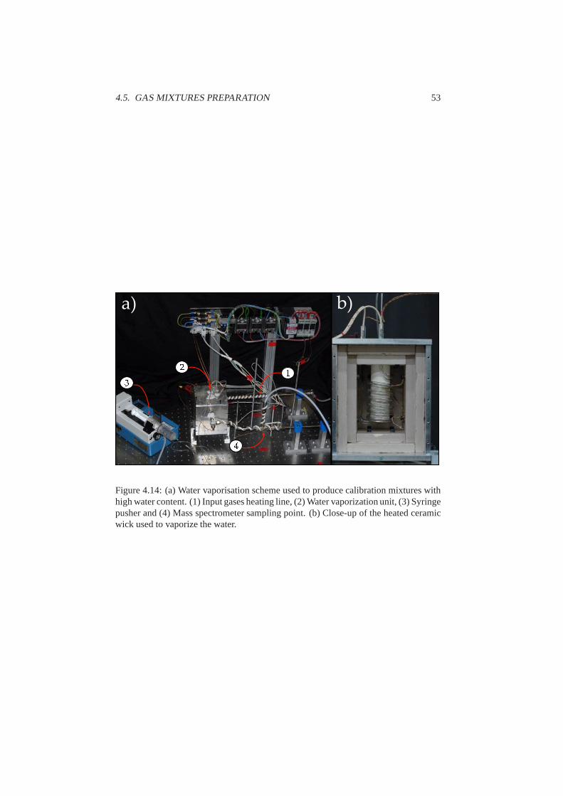
4.5. GAS MIXTURES PREPARATION 53
� �
����
Figure 4.14: (a) Water vaporisation scheme used to produce calibration mixtures withhigh water content. (1) Input gases heating line, (2) Water vaporization unit, (3) Syringepusher and (4) Mass spectrometer sampling point. (b) Close-up of the heated ceramicwick used to vaporize the water.


Chapter 5
Mixture compositionmeasurements
The reactant supply method described in section 4.1.1 implies that effective the compo-sition of the mixture injected in the burning chamber will not be knowa priori from thegas streams prescribed at the flow controllers. The determination of the initial mixturestrength requires the measurementin situ of the mixture composition at the burningchamber boundaries.
5.1 The choice of experimental technique
To measure the effective mixture composition it was first necessary to identify a suit-able experimental technique. The field of analytical chemistry provides many instru-mental means to obtain a quantitative measurement of the composition of a gas sample.The choice of a particular technique was guided by the following factors:
• Low perturbation of the flame. The sampling of the gas mixture must notsignificantly affect the gas flows to the flame, which are on theorder of5 � 10
SLPM.
• Precision. Should obviously be as good as possible, a few % error (2 � 5%)would be acceptable.
• Repetition rate. Since the whole burning chamber will have to be scanned mul-tiple times, one data point should be collected in a few minutes at the most.
• Cost
The instruments commercially available from manufacturers intended for this taskrely on various principles to extract information from the sample. Generally, the sampleis subjected to a stimulus and then a transducer captures itsresponse to be analyzed.For gas mixture composition measurements, most instruments rely on electromagneticradiation (spectroscopy), electric and magnetic fields (mass spectrometry), separation(chromatography) or a combination of these techniques to probe the sample.
Fourier transform infrared spectroscopy (FTIR) was initially considered becauseof its wide availability and simplicity. The optical natureof the instrument allows for
55
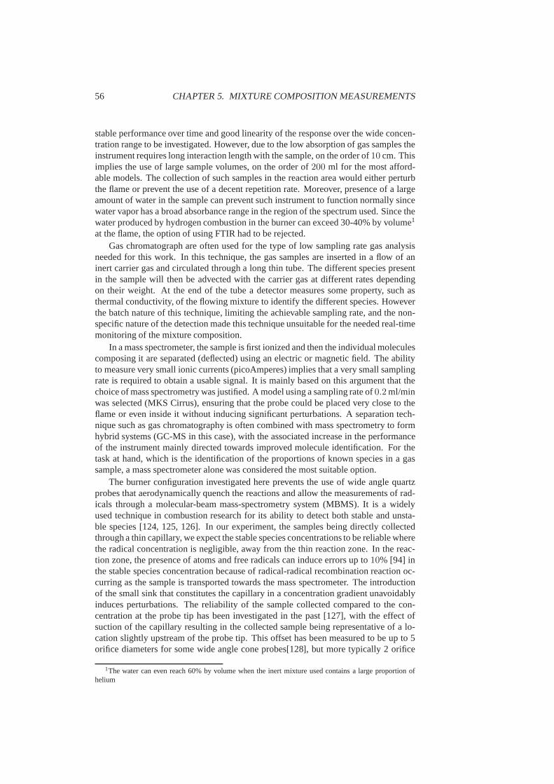
56 CHAPTER 5. MIXTURE COMPOSITION MEASUREMENTS
stable performance over time and good linearity of the response over the wide concen-tration range to be investigated. However, due to the low absorption of gas samples theinstrument requires long interaction length with the sample, on the order of10 cm. Thisimplies the use of large sample volumes, on the order of200 ml for the most afford-able models. The collection of such samples in the reaction area would either perturbthe flame or prevent the use of a decent repetition rate. Moreover, presence of a largeamount of water in the sample can prevent such instrument to function normally sincewater vapor has a broad absorbance range in the region of the spectrum used. Since thewater produced by hydrogen combustion in the burner can exceed 30-40% by volume1
at the flame, the option of using FTIR had to be rejected.Gas chromatograph are often used for the type of low samplingrate gas analysis
needed for this work. In this technique, the gas samples are inserted in a flow of aninert carrier gas and circulated through a long thin tube. The different species presentin the sample will then be advected with the carrier gas at different rates dependingon their weight. At the end of the tube a detector measures some property, such asthermal conductivity, of the flowing mixture to identify thedifferent species. Howeverthe batch nature of this technique, limiting the achievablesampling rate, and the non-specific nature of the detection made this technique unsuitable for the needed real-timemonitoring of the mixture composition.
In a mass spectrometer, the sample is first ionized and then the individual moleculescomposing it are separated (deflected) using an electric or magnetic field. The abilityto measure very small ionic currents (picoAmperes) impliesthat a very small samplingrate is required to obtain a usable signal. It is mainly basedon this argument that thechoice of mass spectrometry was justified. A model using a sampling rate of0.2 ml/minwas selected (MKS Cirrus), ensuring that the probe could be placed very close to theflame or even inside it without inducing significant perturbations. A separation tech-nique such as gas chromatography is often combined with massspectrometry to formhybrid systems (GC-MS in this case), with the associated increase in the performanceof the instrument mainly directed towards improved molecule identification. For thetask at hand, which is the identification of the proportions of known species in a gassample, a mass spectrometer alone was considered the most suitable option.
The burner configuration investigated here prevents the useof wide angle quartzprobes that aerodynamically quench the reactions and allowthe measurements of rad-icals through a molecular-beam mass-spectrometry system (MBMS). It is a widelyused technique in combustion research for its ability to detect both stable and unsta-ble species [124, 125, 126]. In our experiment, the samples being directly collectedthrough a thin capillary, we expect the stable species concentrations to be reliable wherethe radical concentration is negligible, away from the thinreaction zone. In the reac-tion zone, the presence of atoms and free radicals can induceerrors up to10% [94] inthe stable species concentration because of radical-radical recombination reaction oc-curring as the sample is transported towards the mass spectrometer. The introductionof the small sink that constitutes the capillary in a concentration gradient unavoidablyinduces perturbations. The reliability of the sample collected compared to the con-centration at the probe tip has been investigated in the past[127], with the effect ofsuction of the capillary resulting in the collected sample being representative of a lo-cation slightly upstream of the probe tip. This offset has been measured to be up to 5orifice diameters for some wide angle cone probes[128], but more typically 2 orifice
1The water can even reach 60% by volume when the inert mixture used contains a large proportion ofhelium

5.2. MASS SPECTROMETRY BASED PPA 57
diameters[129, 130]. For the straight capillary used in this experiment, we expect theperturbation to be of the same magnitude or smaller and the sampling system to deliverrepresentative samples of stable species immediately in front of the probe tip, whichhas a0.1 mm inner diameter.
5.2 Mass spectrometry based partial pressure analyzer
The instrument used for gas analysis is a compact quadrupolemass-spectrometer (QMS)based residual gas analyzer (RGA) or partial pressure analyzer (PPA). This type of in-strument is used extensively for measuring the compositionof gas samples in indus-trial settings. Their low cost, ease of use and wide application range has lead to theirwidespread adoption in applications where qualitative data is sought, i.e. to assess theintegrity of vacuum systems [131], detect the presence of contaminants in semiconduc-tor manufacturing [132, 133] or monitor chemical processesfor deviation from optimaloperating parameters [134, 135].
The response of PPAs for a particular mass-to-charge ratio (m2z) is usually as-sumed to be a linear function of the partial pressure of the species with massm in thesample, provided that there is no overlapping peaks. The validity of this assumption islimited by the precision expected from the measurements andmust be investigated toensure proper interpretation of the results. For the applications mentioned above, theconcentration of the species of interest varies only in a narrow range in an otherwiseconstant mixture. Accordingly, the assumption of linearity is usually reasonable andcan yield results accurate within a few percent [134] at bestfollowing proper calibra-tion.
On the other hand, the use of PPAs to gather quantitative composition data for ar-bitrary mixtures of a given number of species is much more limited. While trivial tointerpret for qualitative analysis, the instrument response necessitates extensive calibra-tion to yield useful quantitative results. The interpretation of the data is complicatedby the numerous factors that can compromise the instrument linearity when varyingmixture composition over a wide concentration range. In this thesis, a custom calibra-tion procedure is developed to account for the intrinsically non-linear behavior of theQMS response over a wide concentration range in a complex mixture of reactive gases,drastically improving measurement precision.
5.3 The instrument working principles
The working principles of mass spectrometry are considerably more complicated thanfor techniques based on interaction of the sample with electromagnetic radiation (spec-troscopy). A mass spectrometer is made from three basic units: a ion source, a massanalyzer and a detector. A schematic representation is presented in figure 5.1. In orderto properly calibrate the instruments and interpret its results, it is essential to prop-erly understand these basic units. The mass spectrometer used throughout the currentinvestigation presented here is manufactured by MKS Instruments Inc.(Andover, Ma,USA) . The Cirrus mass spectrometer is a bench-top unit that can only be controlledremotely by a computer through an Ethernet connection. A picture of the instrument ispresented in figure 5.2(a). The assembly is built around a Microvision plus IP ResidualGas Analyzer (RGA). A view of the opened instrument identifying various componentsis presented in figure 5.2(b).

58 CHAPTER 5. MIXTURE COMPOSITION MEASUREMENTS
Ion Source Mass Filter Detector
GasSample
DataTreatment
Molecules
Ions Ions
e current-
Figure 5.1: Outline of the different components involved inthe mass spectrometerfunction.
� �
Figure 5.2: (a) Picture of the MKS Cirrus RGA used in this thesis. (b) View of theopened instrument with: (1) the oven enclosure; (2) Bypass line; (3) the capillary inlet;(4) high vacuum chamber housing the ion source and mass filter; (5) detector andassociated electronics.
The sensitivity of the instrument is defined as the magnitudeof the output signalper unit of the quantity measured. For PPA, this quantity is therefore expressed as theionic current detected per unit of pressure of the species measured. Accordingly, theunits used will either be Amperes per Pascals or Amperes per millibars. The instrumentsensitivity is expected to be constant, producing a linear response as a function of thepartial pressure, but in practice this is not the case. This is especially significant overthe wide concentration ranges measured in this work. Various phenomena can inducesnon-linearities in each component of the instrument and in order to achieve a suitablecalibration, these need to be understood. The calibration strategy will aim at estab-lishing the instrument sensitivity separately for all species of interest and as a functionof the factors that were found to be relevant (mixture composition, operating parame-ters). Because of limited access to the system internal states (operating pressures, ioncurrents) and for simplicity, the procedure described in section 5.4 calibrates the in-strument as a whole without separating the different components. The possible origin

5.3. THE INSTRUMENT WORKING PRINCIPLES 59
of these non-linearities of the mass-spectrometer will be discussed in the individualcomponents described in the following sections.
5.3.1 Sampling
The sample is collected through a fused silica capillary, which can be heated to preventcondensation and the resulting flow perturbations. The sampling rate is a function ofthe diameter and length of the capillary used. For the results presented here, the capil-lary diameter was 100µm and its length was230 cm. The resulting flow rate removedfrom the burning chamber was small enough to never induce observable perturbationson the flame. This issue is further discussed in appendix A. The capillary exits in avacuum chamber housing the RGA that is purged by a turbomolecular pump backedby a dry diaphragm pump. The diaphragm pump also serves as a by-pass pump forthe capillary aspiration and ensures a pressure sufficiently low at the entrance of thehigh vacuum vessel. The whole vacuum chamber is housed in an oven to help watervapor removal after startup (bake setting,180XC) and pumping efficiency throughoutnormal operation (warm setting,80XC). This arrangement is visible in figure 5.2(b)and a detailed schematic representation is provided in appendix A.
The sample collected is representative of the composition immediately in front ofthe sampling point. Particular attention was taken to properly characterize the flowregimes present in the different components of the system toavoid mass separationeffects, or fractionation. A detailed analysis of the system used is presented in ap-pendix A. Readers interested in sampling issues in PPA are directed to the exhaustivereview paper of Blessing et al.[136]. The very small sampling rate (0.2 ml/min) re-sults in the conditions throughout the capillary being laminar (Re � 4.9) and subsonicMa � 1.59�10�3. From the estimated pressure distribution in the sampling system,theintermolecular forces are important and the flow can be considered viscous. Therefore,no mass separation effect is expected in the mixture. The conductance of such capillar-ies operating in the viscous regime, given by equation A.6 isthe same for every species.Accordingly, the composition in the bypass chamber is identical to the composition atthe sampling point since the flow is viscous in both the input capillary and the bypassline.
5.3.2 The ion source
In the MKS Cirrus, part of the sample is ionized in the ion source through electron im-pact ionization (EI). Electron ionization is a common technique in mass spectrometry,especially when dealing with gas samples with unknown organic molecules. Electronsare produced by heating a tungsten filament (thermionic emission) and then acceler-ated towards the sample by a static electric field. The samplemolecule or atomM isionized following relation 5.1.
M � e� �M� � 2e� (5.1)
The proportions of sample molecules that will be ionized will vary greatly depend-ing on many parameters and will be a great source of variability in the calibrationprocedure. These include the specie nature (weight, diameter, etc.), its partial pressure,the total pressure, the electron energy, the presence of reactive species in the chamber,the state of the filament (age, surface adsorption of certainspecies, etc.) and manyothers to a lesser extent. For the particular model used here, the ion source comprises

60 CHAPTER 5. MIXTURE COMPOSITION MEASUREMENTS
two tungsten filaments located close to each other. The particular filament used willhave an influence on the electrons trajectories and hence on the ionization efficiency.To ensure stable operation, ion source design has to accountfor physical phenomenathat can affect electron production.
As they are used, the filament lose material to evaporation. This loss of surfacearea means that the filament has to be operated at a higher temperature to supply thesame electron current. Although the emission current is regulated automatically andin real time to account for the variation in the filament performance, the ionizationefficiency can vary significantly over the course of a measurement. In this paper, weare mainly interested in the effect of mixture composition on EI efficiency. It hasbeen known for a long time that the presence of even a small amount of gas around athermionic cathode induces strong species-specific emission changes[137]. Over thecourse of our experiments two time scales have been noticed in the variation of theinstrument performance: upon mixture composition change,some changes occurredover the course of a few seconds or minutes, while others tookhours to set it. Recentexperimental evidence [138] demonstrate that the nature ofthe gas species presentin the vacuum chamber can also affect the work function of thethermionic emitterthrough diffusion in the filament material. The nature of theatoms adsorbed on theemitter surface is also believed to play a role. These phenomena imply that even ifthe ionization current is monitored and regulated, the energy of the electrons and thefocusing of the ions vary with the mixture composition. Thisvariation in the ionizationefficiency of the source necessitates proper calibration toallow the instrument to beoperated over a wide mixture composition range.
It has been shown that space charge effects can account for the almost instanta-neous change in instrument sensitivity when the mixture composition is changed. Thespace charge effects can change both the local potential in the ionization chamber andthe efficiency of ions focusing towards the mass filter [139, 140, 141]. This effect de-pends strongly on the geometry of the ion source and is therefore instrument specific.It is however found to some extent in all commercial mass spectrometers [142]. Spacecharge effects can also become significant when the absolutepressure in the vacuumchamber is increased while the mixture composition remainsconstant. This effect isprobably the most investigated mass spectrometer nonlinearity [143, 142, 140, 134].For the experiments presented here, the very small and constant leak rate into the vac-uum chamber ensured that the pressure remained more or less constant, see appendixA for details. The small measured pressure changes2 observed while the mixture com-position was changed are attributed to the ionizing nature of the total pressure gaugeused (Penning gauge). Accordingly, the calibration presented here do not include theeffect of high pressure on the instrument sensitivity.
The introduction of reactive gases in the vacuum chamber causes, in addition tothe short timescale phenomena mentioned above, a slow driftin the instrument re-sponse. Oxidation and evaporation of material from the filament [144, 145] shouldnormally be compensated by the electronics regulating the electron emission. On theother hand, the adsorption of molecule on the source surfaces can have reversible ef-fects on the order of 10% with timescales of hours [142, 134] following even briefexposure to reactive gases. Over the course of weeks or months of operation, ionsource and mass filter fouling can also induce significant variation in the instrumentsensitivity through the deposition of insulating films on conductors or conducting films
2The Cirrus model allows the monitoring of the vacuum chamberpressure in real time while the experi-ments are conducted.

5.3. THE INSTRUMENT WORKING PRINCIPLES 61
on insulators [143, 142, 146], modifying the source optics.These long timescales ef-fects collectively known as source fouling will be addressed by the implementation ofa calibration transfer strategy [147, 146], described in section 5.4.2.
5.3.3 The mass analyzer
To separate ions based on their mass-to-charge ratio, a quadrupole arrangement is used.The RF (radio frequency) oscillating electric field it produces deflects the ions differ-ently depending on their mass-to-charge ratio (m2z). The quadrupole is designed insuch a way that for a given frequency only ions with a singlem2z ratio will reachthe detector. The variation of this frequency across a certain range generates a signalreaching the detector that is representative of a succession of m2z ratios. The resultingscan is the mass spectrum of the species present in the sample. The mass filter usedin the Cirrus is able to filter ions having a mass from 2 to 200 amu. The transmissionefficiency of the quadrupole mass filter is known to be strongly mass dependent, up to afactor 5 [142]. This effect will be addressed by the calibration procedure implementedin section 5.4.2.
Some ambiguity may arise if two species present in the samplehave the samem2zratio, for instance carbon monoxide and molecular nitrogen(mass 28). The electronimpact ionization can also result in the fragmentation of target molecules, producingnew species that can overlap with species of interest. Cracking tables provided by themanufacturer or found in the literature can be used to determine the height of thesesecondary peaks from the main ones to resolve the ambiguity.In the results presentedhere the only instance where this was necessary was when measuring molecular oxygenand methane simultaneously. The fragmentation of O2 upon ionization produces asecondary peak of mass 16 (11% of the height of the main peak),corresponding toatomic oxygen that must be subtracted from the methane peak to get its true value.
All of the ions whosem2z ratios are discarded by the mass filter end up their courseson the quadrupole rods where they recombine with electrons.When measuring certainspecies, especially large hydrocarbons, this can result ina surface fouling phenomenonsimilar to the one described in the previous section. Because of the nature of the speciesmeasured in this experiment, this effect is not expected to be important. In any case, theresulting long term sensitivity drift will be corrected by the calibration transfer strategydescribed in section 5.4.2.
5.3.4 The detectors
The sensitivity of the ion detector itself is also subject tovariations over time. TheCirrus instrument used here is equipped with two types of detectors: A Faraday cupand a secondary electron multiplier (SEM).The Faraday cup detector is the most stabledetector type, with the observed sensitivity changes for some instruments as low as10% over months of use [134]. The more sentitive SEM detectoris considerably lessstable, especially when new, with order-of-magnitude variations observed over the firstfew weeks of use [142].
The SEM detector is significantly more sensitive that the Faraday cup, allowingdetection levels in the low parts per millions (ppm) to hundreds of parts per billion(ppb) for the type of instrument used. However, the most sensitive detectors are usu-ally the most non-linear [134]. Consequently, for all of themeasurements presentedhere, only the Faraday cup detector was used because ppm detection levels were not

62 CHAPTER 5. MIXTURE COMPOSITION MEASUREMENTS
required. This simplified the calibration by removing the detector voltage as a parame-ter and was more than enough for the parts per thousand precision expected from thesemeasurements.
5.3.5 Control software
To interface with the RGA, MKS supplies a software namedProcess Eye. This soft-ware isrecipe-based, which means that the instrument is not controlled directlyby theuser but rather through a file (the recipe) containing a set ofinstructions. The languageused is Visual Basic for applications (VBA) but the user is discouraged edit or evenlook at the code and directed to thesoftware wizardfor the creation of the recipes.This interface only allows the creation of very basic tasks for the instrument, such asmeasuring specific ranges of masses for a given time intervaland performing basicdata treatment. Thewizard then writes the code for the recipe and that’s it as far as theaverage user is concerned. When the instrument is started, the software reads the sup-plied recipe file and follows the instructions supplied therein. The wizard only allowsthe measured data to be provided graphically to the user or saved to a proprietary fileformat and is always in units of pressure. The user software does not provide meansto access, let alone control, the instrument operating parameters such as the measuredcurrents.
The implementation of the more complex tasks expected of this instrument in theresearch context in which it is used was a monumental task. For instance, the calibra-tion of the instrument described in the next section calls for the relationship betweenthe input (the partial pressure of a specific species) and theoutput (the measured cur-rent) to be established. Thewizard was completely useless for this task since it doesnot even allow the knowledge of the measured current, it is supplied to the user al-ready converted to a partial pressure, with the intermediate steps unspecified. All ofthe recipes used were therefore coded by hand and since the user is not expected to beable to write de code, documentation was very scarce.
The software reference supplied with the product contains only information on howto use thewizard which, needless to say, is a disappointment. The most usefuldocu-mentation obtained from the manufacturer is a scriptable object reference. It lists thename of the software object used to control the instrument, its inputs and its outputs.Unfortunately, it only lists the names of the object, not their authorized values nor theirdescription. A lot of trial and error was therefore involvedin getting anything to workat all. A more exhaustive reference intended for applications developers using this soft-ware was later acquired: the software development kit (SDK)reference manual for theProcess Eyesoftware. It included a more detailed reference of some the scriptable ob-jects but proved of limited use for the understanding of the instrument control, behaviorand responses.
In the end, the use of software and the instrument in general was a horrible ex-perience. The writing of recipe files was a tedious task and necessitated endless trialand errors to achieve the desired outcome. Over 15’000 linesof code where writtenthroughout this project only to achieve the calibration of the instrument, a task thateasily swallowed the equivalent of six months of full-time work. The technical sup-port staff at MKS was usually very friendly and helpful to answer specific questions,once they were identified. However, most of the time their answers to more generalquestions were that they don’t know because the instrument and software were simplynever intended for such tasks. The software is only aimed at providing a clueless userthe ability to monitor small changes from a reference state in a mixture containing only

5.4. MASS SPECTROMETER CALIBRATION 63
trace amounts of one specie of interest. Everything else is uncharted territories and hadto be characterized for this specific instrument. I will end my rant now, I just wantedto point out that I hate this machine and especially its control software.
5.4 Mass spectrometer calibration
The issue faced when wanting to use a atmospheric pressure RGA such as the MKSCirrus to perform quantitative mixture composition is one of purpose. The instrumentis intended to measure small variation in species themselves present in a small quan-tity diluted in a more or less constant gas matrix (hence the nameresidual). In theseconditions, it is reasonable to expect the instrument response to be a linear function ofthe amount of the species of interest present. To calibrate the instrument, one mixtureclose what is typically encountered in practice and containing all the species of interestshould be sufficient. In the current work, the mixtures encountered have a wide con-centration range, i.e. the composition of the gas matrix is the subject of interest. As aresult, significant non-linearities arise in different parts of the instrument (ion source,mass filter, detector) and need to be calibrated extensively. In the following sectionswill be discussed first the calibration procedures suppliedby the instrument manufac-turer and then the one implemented to account for the observed non-linearities.
5.4.1 Built-in procedure
The calibration procedure built-in the MKS mass spectrometer proved very disappoint-ing, to the point that the results initially gathered were unusable for their intended pur-pose. As it is delivered, the only available calibration procedure implemented involvesdetermining the instrument sensitivity by measuring a single reference sample. Theuser has to supply the molecular mass of one of the species present in the sample andits partial pressure. The software then simply divides the measured signal by the sup-plied partial pressure to obtain a calibration factor, in amperes per unit of pressure (themillibar or the Pascal were used here). This calibration factor is the instrument sensi-tivity for the specific species used in the calibration underthe conditions prevalent atthe time. Thissinglecalibration factor was then used by the software to calculate thepartial pressure ofeveryspecies undereveryconditions. As it is delivered, the instru-ment is therefore assumed to have a constant sensitivity as afunction of the analyzedmass and a linear response over its dynamic range.
Tillford [134] noted in his paper on the limiting factors in the use of RGA forprocess monitoring, that users and some manufacturers assume that the same relativesensitivities used in ionization gages can be used for RGAs.However, this shortcutfails to account for the mass dependence of the different constituents of the RGA sys-tem listed in sections 5.3.1 to 5.3.4. For instance, in this same paper, the mass filtertransmission dependence on the mass of the ions measured changes the RGA sensitiv-ities by a factor 5 to ten compared to the ionization gages relative sensitivities. Theshortcomings of these simplistic assumptions soon proved significant when measuringthe mixtures encountered in this experiment.
When analyzing initial measurements made using the instrument calibrated fol-lowing the built-in procedure, outrageous errors were noticed if the measured mixturedeviated from the one used for the calibration. Moreover, the sensitivities for differentspecies measured in pure samples is drastically different,with one order of magnitudebetween the sensitivity of hydrogen and that of CO2. Further investigations revealed a

64 CHAPTER 5. MIXTURE COMPOSITION MEASUREMENTS
strong variation of the instrument sensitivity as a function of the mixture content beinganalyzed. For instance, the sensitivity of the instrument to hydrogen doubles betweena mixture containing only trace amounts of the gas in an argonmatrix and an evenmixture of the two gases. When concentration profiles are taken along the burner lon-gitudinal axis, the fuel concentration varies from typically 15 � 30% to trace amountsand errors in excess of100% can result from the use of a constant calibration factor.The effect was a little less pronounced for oxygen, and as lowas about20% for CO2.Nevertheless the cumulative effect on the measurement of the mixture strength, whichis the main task that the instrument is intended for, is nothing short of catastrophic.
From that point, it was clear that this specific mass spectrometer would be uselessin this experiment without the implementation of an extensive calibration procedure.This will make the instrument more versatile, allowing to gobeyond the assumption oflinear response. Although simplistic, this assumption is nevertheless valid for the actualpurpose this instrument is designed for. That is the on-linemonitoring and analysis ofgas mixtures including trace contaminants in process gases.
5.4.2 Calibration over a wide concentration range
The objective of the calibration procedure implemented here is to capture the instru-ment response for each species of interest as a function of the operating parametersand the mixture composition in which the measurements are conducted. This is donethrough the measurement of numerous reference mixture of different compositions, re-ferred to as thetraining set. The result is multidimensional mapping of the instrumentsensitivity, with the number of dimensions equal to the number of gases in the mix-ture minus one3. One of these maps has to be generated for each species of interestand each set of operating parameters of the instrument. The parameters that should beconsidered include the ionization current, the extractionpotential, the filter voltage andthe detector gain. For the sake of simplicity, after the optimal operating conditions hadbeen found, all of the instruments settings were kept constant.
Since the extent and nature of the non-linearities in the response of QMSs is poorlydocumented and instrument specific, it was difficult to defined an optimized trainingset beforehand. Therefore, the initial treatment of the problem involved a large amountof different mixtures spread over the entire concentrationspace of interest. Efforts toreduce the training set to a minimum required by the nature ofthe instrument responsecan then be made for further calibrations. An experimental set-up had to be constructedthat could provide a wide range of reference mixtures of the species of interest, which ispresented in section 4.5. For the CO2-diluted H2-O2 flames studied, the concentrationspace of interest is 0-100% for CO2, 0-75% for O2 and 0-50% for H2, H2O.
Calibration transfer
The term calibration transfer applies to methods aiming to establishing the current be-havior of an instrument through a limited number of measurements, referred to as thetransfer set, by transferring the knowledge of the instrument behavior gained using anextensive training set[148, 147, 146]. For the procedure implemented here, correctionfactors are determined for each species of interest by comparing the measured sen-sitivities from similar mixtures in the transfer and initial training set. It is assumed
3One dimension can be removed because we assumed that all gases present in the sample are measured.This allows the total of all the measured mole fractions to beset to 1 and an arbitrary species concentrationto be considered a dependent variable.

5.4. MASS SPECTROMETER CALIBRATION 65
that these effects while affecting eachm2z ratios differently, hence the species specificcorrection factors, do not affect the interactions betweenthe species. The sensitivitymaps themselves are therefore retained from the initial training set and the correctionsimply applied as an offset. This account for the variationsin instrument sensitivitythat occurred since the initial calibration. Experimentalresults on two and three gasmixtures confirm that this assumption is reasonable becausealthough the height of re-sponse surface changes over the course of weeks, its shape remains unchanged. Thistemporal drift in the instrument response is present in all QMS instruments and be-comes significant over the course of days to weeks, dependingon the nature of themixtures measured.
In the present experiment, the transfer set was simply the species of interest eitherpure (for CO2) or at the upper bound of their calibrated range (75% for O2, 50% for H2
and H2O) diluted in CO2. This allowed the calibration of the instrument to be refresheddaily from the measurement of only four simple mixtures.
Binary mixtures
The response of the instrument was first measured when exposed to various binarymixtures of the species of interest diluted in a inert gas. Argon was chosen since it isvery stable and extensive literature for the mass spectrometric measurement is availableon this species. The variation of the instrument sensitivity, in Amperes per Pascals4 ispresented in figure 5.3 for the first three species of interest(H2, O2 and CO2). Sincesome of these measurements series were taken on different days, the calibration trans-fer strategy described above has been implemented to match the sensitivities of puresamples.
3⋅10-12
4⋅10-12
5⋅10-12
6⋅10-12
7⋅10-12
8⋅10-12
0 20 40 60 80 100
Sen
sitiv
ity [A
mp/
mba
r]
Argon vol. fraction [%]
3⋅10-12
4⋅10-12
5⋅10-12
6⋅10-12
7⋅10-12
8⋅10-12
0 20 40 60 80 100
Sen
sitiv
ity [A
mp/
mba
r]
Argon vol. fraction [%]
3⋅10-12
4⋅10-12
5⋅10-12
6⋅10-12
7⋅10-12
8⋅10-12
0 20 40 60 80 100
Sen
sitiv
ity [A
mp/
mba
r]
Argon vol. fraction [%]
(a)
1⋅10-12
2⋅10-12
3⋅10-12
4⋅10-12
5⋅10-12
6⋅10-12
0 20 40 60 80 100
Sen
sitiv
ity [A
mp/
mba
r]
Vol. fraction [%]
1⋅10-12
2⋅10-12
3⋅10-12
4⋅10-12
5⋅10-12
6⋅10-12
0 20 40 60 80 100
Sen
sitiv
ity [A
mp/
mba
r]
Vol. fraction [%]
1⋅10-12
2⋅10-12
3⋅10-12
4⋅10-12
5⋅10-12
6⋅10-12
0 20 40 60 80 100
Sen
sitiv
ity [A
mp/
mba
r]
Vol. fraction [%]
(b)
Figure 5.3: Mass spectrometer sensitivity in binary mixtures of H2 (Q), O2 (b), CO2
(2) in Ar. a) Effect of the addition of the other gases on the sensitivity of argon. b)Sensitivity of H2, O2 and CO2 as a function of their volume fraction..
It can be seen from the results presented in figure 5.3(a) thatthe presence of hy-drogen in the sample increases the sensitivity of the instrument for argon while oxygen
4In the determination of the instrument sensitivities, the atmospheric pressure is used as the referencestate. This implies that the pressure drop in the sampling capillary is included in the calibration factor. Themeasured non-linearities are therefore the sum of the contributions of each component in the system, fromthe gas molecules sampled to the electrons counted at the other end. The interested reader is referred toappendix A for an analysis of the sampling and ionization part of the system.

66 CHAPTER 5. MIXTURE COMPOSITION MEASUREMENTS
decreases it. CO2 has a small positive effect on the sensitivity, but less pronouncedthat for the two other species. To understand this phenomena, it should be noticedfrom figure 5.3(b) that the magnitude of the sensitivities differs significantly betweenthe species. For instance, the sensitivity of the instrument to hydrogen is about 5 timessmaller than for argon. Therefore, as the argon is replaced by hydrogen in the sample,the charge density in the ionization chamber and mass filter decreases. This hints to-wards space charge effects being one of the causes of the observed mixture dependenceof the instrument sensitivity. The effect of water, the fourth species of interest, is shownin figure 5.4. As water added in a CO2 sample, it can be seen that the sensitivity of boththe H2O and the CO2 decreases. The phenomenon is similar in nature and magnitudeto what was previously observed in O2 and mixtures of argon.
1.0⋅10-12
1.5⋅10-12
2.0⋅10-12
2.5⋅10-12
3.0⋅10-12
0 20 40 60 80 100
Sen
sitiv
ity [A
mp/
mba
r]
Vol. fraction [%]
1.0⋅10-12
1.5⋅10-12
2.0⋅10-12
2.5⋅10-12
3.0⋅10-12
0 20 40 60 80 100
Sen
sitiv
ity [A
mp/
mba
r]
Vol. fraction [%]
Figure 5.4: Mass spectrometer sensitivity variation in thepresence of a variable amountof H2O (b) in a CO2 (2) matrix.
The presence of O2, H2O and to some extent CO2 in a sample is known to induceoxidation and adsorption on the surface of the instrument exposed to these reactivegases. This results in changes in the properties of these surfaces intervening over thecourse of minutes to hours. When the exposure to the reactivegas is ended, these gasesdesorb from the surface which recovers some if not all of its initial properties. To studythis effect, the composition of a binary mixture of argon andoxygen was changed sev-eral times over the course of a 6 hours period, the results arepresented in figure 5.5.This experiment revealed that after initial exposure to oxygen, the system takes closeto one hour to stabilize within 10% of its final sensitivity. The addition of 10% O2 re-sulted in a 20% decrease of the instrument sensitivity to argon. Subsequent changes inthe oxygen content of the mixture seemed to be equilibrated equilibrated slightly faster.These timescales had to be considered when conducting measurement over large oxy-gen concentration ranges. The sudden drops and recovery in both species sensitivitynoticed between2 and3 hours are of unknown origin and have been observed spo-radically. The global effect of these variation suggest that they are perhaps caused bypartial and temporary blockage of the sampling system. In the event that such a varia-tion were to become permanent, the calibration transfer procedure described in section5.4.2 ensures that the instrument response is updated frequently.

5.4. MASS SPECTROMETER CALIBRATION 67
1⋅10-13
2⋅10-13
3⋅10-13
4⋅10-13
5⋅10-13
6⋅10-13
Sen
sitiv
ity [A
mp/
mba
r]
1⋅10-13
2⋅10-13
3⋅10-13
4⋅10-13
5⋅10-13
6⋅10-13
Sen
sitiv
ity [A
mp/
mba
r]
0255075
100
0 1 2 3 4 5 6% A
r
Time [hours]
Figure 5.5: Time dependence of instrument sensitivity in a binary mixture of argon (2)and oxygen (X).Mixtures of three and four gases
In the simplest experiments presented in this thesis, the number of species present in theburning chamber is four and include both reactants, a singleproduct and the inert. Toproperly characterize the mass spectrometer in this three-dimensional parameter space,a large number of reference mixtures evenly distributed in the region of interest weregenerated. For the measurements of concentration profiles in hydrogen-oxygen flamesdiluted in CO2, the ranges of interest are0-50% for H2, 0-50% for H2O, 0-75% for O2
and0-100% for CO2. For obvious reasons, an automated mixture generation setup wasdeveloped and is described in section 4.5. Mapping the sensitivity of the instrument inthree gas mixtures (without water) using49 reference composition sampled about30
minutes each took a little over a day of measurements. An example of the sensitivitydependence in such a three gas mixture is presented in figure 5.6.
The addition of the fourth species to the mixture required the development of aprecise water vaporization unit, described in section 4.5 to supply a controlled flow rateof water vapor to a heated mixture of the other three gases. The three gas proceduredescribed above was then repeated 4 times with a different amount of water vaporto cover the range of interest for this species. This four gascalibration procedurerequired an extensive amount of time to be completed. Accordingly, to reduce theinfluence of the long term drift of the instrument on the accuracy of the calibration, thenumber of mixtures measured for each water concentration was decreased to36 andthe measurement time to20 minutes. With these measures it was possible to completethe whole four-gas calibration in just under48 hours. To ensure that the instrumentlong term drift did not induce a bias in the measurements, a pure sample of one of thespecies of interest was measured at regular intervals in theprocedure to monitor theevolution of the absolute sensitivity. Unfortunately, thedevice available to supply theliquid water to the apparatus (a medical syringe pusher) required human interventionthroughout this lengthy calibration process. It was necessary to change the syringeabout every hour and manually set the flow rate, preventing the implementation of atruly automated procedure.

68 CHAPTER 5. MIXTURE COMPOSITION MEASUREMENTS
010
2030
4050
010
2030
4050
6070
1.0⋅10-14
1.5⋅10-14
2.0⋅10-14
2.5⋅10-14
3.0⋅10-14
H2
sens
itivi
ty [A
mp/
Pa]
% H2% O2
1.0⋅10-14
1.5⋅10-14
2.0⋅10-14
2.5⋅10-14
3.0⋅10-14
010
2030
4050
010
2030
4050
6070
1.0⋅10-14
1.5⋅10-14
2.0⋅10-14
2.5⋅10-14
3.0⋅10-14
H2
sens
itivi
ty [A
mp/
Pa]
% H2% O20
1020
3040
50
010
2030
4050
6070
1.0⋅10-14
1.5⋅10-14
2.0⋅10-14
2.5⋅10-14
3.0⋅10-14
H2
sens
itivi
ty [A
mp/
Pa]
% H2% O2
(a) H2
010
2030
4050
0102030405060701.2⋅10-13
1.4⋅10-13
1.6⋅10-13
1.8⋅10-13
2.0⋅10-13
O2
sens
itivi
ty [A
mp/
Pa]
% H2
% O2
1.2⋅10-13
1.4⋅10-13
1.6⋅10-13
1.8⋅10-13
2.0⋅10-13
010
2030
4050
0102030405060701.2⋅10-13
1.4⋅10-13
1.6⋅10-13
1.8⋅10-13
2.0⋅10-13
O2
sens
itivi
ty [A
mp/
Pa]
% H2
% O2
010
2030
4050
0102030405060701.2⋅10-13
1.4⋅10-13
1.6⋅10-13
1.8⋅10-13
2.0⋅10-13
O2
sens
itivi
ty [A
mp/
Pa]
% H2
% O2
(b) O2
010
2030
4050
0102030405060702.0⋅10-13
2.3⋅10-13
2.5⋅10-13
2.8⋅10-13
3.0⋅10-13
CO
2 se
nsiti
vity
[Am
p/P
a]
% H2
% O2
2.0⋅10-13
2.3⋅10-13
2.5⋅10-13
2.8⋅10-13
3.0⋅10-13
010
2030
4050
0102030405060702.0⋅10-13
2.3⋅10-13
2.5⋅10-13
2.8⋅10-13
3.0⋅10-13
CO
2 se
nsiti
vity
[Am
p/P
a]
% H2
% O2
010
2030
4050
0102030405060702.0⋅10-13
2.3⋅10-13
2.5⋅10-13
2.8⋅10-13
3.0⋅10-13
CO
2 se
nsiti
vity
[Am
p/P
a]
% H2
% O2
(c) CO2
Figure 5.6: Mass spectrometer sensitivity in H2-O2-CO2 mixtures. When the total ofthe volume fractions of the two species given on the base axesof the graph do not equal100%, the remainder is CO2.
Extension to more complex mixtures
To produce the wide ranges Lewis numbers necessary for the work presented here, asecond inert must be added to the mixture. This means that theminimum number ofspecies present in the burner climbs to five. From practical considerations it is evidentthat the calibration procedure described previously cannot be extended in its currentform from four to five species. The time required to map such a complex parameterspace implies that the state of the instrument cannot be assumed constant throughoutthe procedure. Accounting for this drift effect would add another level of complicationto a process that does not need it.
The extension of the method to more complex gas mixtures therefore requires theuse of a certain number of simplifying assumptions. The simplest solution would be toconstruct a multi-dimensional mapping of the instrument sensitivity from elementaryknowledge gained in simple mixtures. Using the results frombinary mixtures it ispossible to quantify the effect that the concentration of a given gas has on the sensitivityof other gases. This approach was tested on the three gas mixtures presented in figure5.6. However, no trick was found to account for the differenteffect of one gas onanother as a function of the concentration of a third. It is believed that the interactionsbetween the species are too important for such a simple approach to be effective.
One simplification can be found by exploiting the limit of infinitely fast combustionwhich specifies that the advected reactant should be consumed entirely at the flame. Inthe absence of leakage both reactants should therefore never be present simultaneouslyin any great amount at the same location in the burner. Each reactant can then be

5.4. MASS SPECTROMETER CALIBRATION 69
calibrated separately with the two inerts using the three gas procedure described previ-ously. The effect of the product, water in this case, can be dealt with in the same fashionas previously, resulting in a mere doubling of the length of the calibration procedurefrom the four to the five gas scenario. Further simplificationis possible by consideringthe effect of water as a multiplying factor applied on top of the three gas sensitivitymaps available for each domain of the burner. The effect of the water concentrationon the sensitivity of other gases can be derived from graphs such as the one presentedfor CO2 in figure 5.4. This requires the assumption that the relativeeffect of H2O onthe instrument sensitivity is the same for every species which was measured to be rea-sonable for the H2O range investigated here. The choice of the dataset to use for themixture analysis will then be dictated by which of the reactants is present in the largestamount. The sensitivity of the scarce reactant was estimated from the other dataset bytaking into account the general effect of the abundant reactant on other species.
The choice of the second inert to use in the five gas mixture wasfocused on find-ing an inert as light as possible, since it will result in higher Lewis number for thereactants. These high Lewis numbers are required to producemixtures where the dom-inant thermal-diffusive instability mode close to extinction is intensity pulsations. Thisrequirement made the choice of Helium natural. Unfortunately, the use of this gascomplicates the calibration procedure since its very high ionization energy results inextremely low ionization efficiency and sensitivity. For reference, the typical sensi-tivity of helium measured here is1220 that of CO2. The heavy inert used was onlychosen sufficiently different from helium to ensure that therange of Lewis numbersproduced was sufficiently wide to conduct meaningful experiments. Even if CO2 isused in most of the combustion experiments, argon was also investigated because it isof similar weight but is known to be much more simple to measure in mass spectrom-eter systems. Examples of three gas sensitivity maps for both the fuel and the oxidantsides of the burner are presented in figure 5.7 and 5.8, respectively.
The use of helium and argon as the inert mixtures illustratesthe effect of a largechange in the mean proprieties of the mixture on the instrument sensitivity. The mostimportant of these properties appear to be the mass and the first ionization energy. Thegraphs of figure 5.7(a) and 5.7(b) show a factor two change in the sensitivity of H2 andhelium as a function of mixture composition. The lowest sensitivities are associatedwith the highest concentrations of argon in the mixture. Thecalibration of the oxidantside presented in figure 5.8 yield similar results for O2 and helium. A comparisonbetween the two sides reveals that the sensitivity of argon seems to be more affectedby the presence of O2 that that of H2.
5.4.3 Results and discussion
The effectiveness of the calibration method implemented was assessed regularly bymeasuring reference mixtures of known composition. At the beginning of each day ofmeasurement, a reducedtransfer setof mixtures was analyzed to perform the calibra-tion transfer. Following this adjustment, a few other reference mixtures representativeof the experiment being conducted at the time were measured.This provides an esti-mation of the error associated with the current measurements. The results gathered fol-lowing this calibration update and verification routine over the course of2 months arepresented in figure 5.9. These results include the error evaluation for H2, O2, heliumand CO2. The measurement of reference samples containing water vapor generallyyielded an error of about 5% for H2O. The verification of measurements of the sam-ples with a water content was carried out less often that for the other species because

70 CHAPTER 5. MIXTURE COMPOSITION MEASUREMENTS
3.0⋅10-14
4.0⋅10-14
5.0⋅10-14
6.0⋅10-14
0 10 20 30 40 50
025
5075
100 2⋅10-14
3⋅10-14
4⋅10-14
5⋅10-14
6⋅10-14
H2
sens
itivi
ty [A
mp/
Pa]
% H2
% He0 10 20 30 40 50
025
5075
100 2⋅10-14
3⋅10-14
4⋅10-14
5⋅10-14
6⋅10-14
H2
sens
itivi
ty [A
mp/
Pa]
% H2
% He0 10 20 30 40 50
025
5075
100 2⋅10-14
3⋅10-14
4⋅10-14
5⋅10-14
6⋅10-14
H2
sens
itivi
ty [A
mp/
Pa]
% H2
% He
(a)
1.0⋅10-14
1.5⋅10-14
2.0⋅10-14
2.5⋅10-14
3.0⋅10-14
0 10 20 30 40 50
025
5075
100 1⋅10-14
2⋅10-14
3⋅10-14
He
sens
itivi
ty [A
mp/
Pa]
% H2
% He0 10 20 30 40 50
025
5075
100 1⋅10-14
2⋅10-14
3⋅10-14
He
sens
itivi
ty [A
mp/
Pa]
% H2
% He0 10 20 30 40 50
025
5075
100 1⋅10-14
2⋅10-14
3⋅10-14
He
sens
itivi
ty [A
mp/
Pa]
% H2
% He
(b)
5.0⋅10-135.5⋅10-136.0⋅10-136.5⋅10-137.0⋅10-137.5⋅10-13
0 10 20 30 40 50
025
5075
100 5⋅10-13
6⋅10-13
7⋅10-13
Ar
sens
itivi
ty [A
mp/
Pa]
% H2
% He0 10 20 30 40 50
025
5075
100 5⋅10-13
6⋅10-13
7⋅10-13
Ar
sens
itivi
ty [A
mp/
Pa]
% H2
% He0 10 20 30 40 50
025
5075
100 5⋅10-13
6⋅10-13
7⋅10-13
Ar
sens
itivi
ty [A
mp/
Pa]
% H2
% He
(c)
Figure 5.7: Mass spectrometer sensitivity in H2-He-Ar mixtures.
025
5075 0
2550
75100
2.0⋅10-13
3.0⋅10-13
O2
sens
itivi
ty [A
mp/
Pa]
% O2 % He
1.5⋅10-13
2.0⋅10-13
2.5⋅10-13
3.0⋅10-13
025
5075 0
2550
75100
2.0⋅10-13
3.0⋅10-13
O2
sens
itivi
ty [A
mp/
Pa]
% O2 % He
025
5075 0
2550
75100
2.0⋅10-13
3.0⋅10-13
O2
sens
itivi
ty [A
mp/
Pa]
% O2 % He
(a)
025
5075 0
2550
75100
5.0⋅10-15
1.0⋅10-14
1.5⋅10-14
2.0⋅10-14
2.5⋅10-14
3.0⋅10-14
He
sens
itivi
ty [A
mp/
Pa]
% O2 % He
5.0⋅10-151.0⋅10-141.5⋅10-142.0⋅10-142.5⋅10-143.0⋅10-14
025
5075 0
2550
75100
5.0⋅10-15
1.0⋅10-14
1.5⋅10-14
2.0⋅10-14
2.5⋅10-14
3.0⋅10-14
He
sens
itivi
ty [A
mp/
Pa]
% O2 % He
025
5075 0
2550
75100
5.0⋅10-15
1.0⋅10-14
1.5⋅10-14
2.0⋅10-14
2.5⋅10-14
3.0⋅10-14
He
sens
itivi
ty [A
mp/
Pa]
% O2 % He
(b)
3.0⋅10-13
4.0⋅10-13
5.0⋅10-13
6.0⋅10-13
7.0⋅10-13
025
5075 0
2550
75100
3⋅10-13
4⋅10-13
5⋅10-13
6⋅10-13
7⋅10-13
Ar
sens
itivi
ty [A
mp/
Pa]
% O2 % He
025
5075 0
2550
75100
3⋅10-13
4⋅10-13
5⋅10-13
6⋅10-13
7⋅10-13
Ar
sens
itivi
ty [A
mp/
Pa]
% O2 % He
025
5075 0
2550
75100
3⋅10-13
4⋅10-13
5⋅10-13
6⋅10-13
7⋅10-13
Ar
sens
itivi
ty [A
mp/
Pa]
% O2 % He
(c)
Figure 5.8: Mass spectrometer sensitivity in O2-He-Ar mixtures.

5.4. MASS SPECTROMETER CALIBRATION 71
025
5075
100
025
5075
100 0
5
10
15
20R
elat
ive
erro
r [%
]
% He
% CO2
(a) H2
025
5075
100
025
5075
100 0
5
10
15
20
Rel
ativ
e er
ror
[%]
% He
% CO2
(b) O2
025
5075
100
025
5075
100 0
5
10
15
20
Rel
ativ
e er
ror
[%]
% He
% CO2
(c) He
025
5075
100
025
5075
100 0
5
10
15
20
Rel
ativ
e er
ror
[%]
% He
% CO2
(d) CO2
Figure 5.9: Evaluation of the mass spectrometer measurement error after the imple-mentation of the five gas calibration.
of the long startup times associated with the vaporization apparatus.To determine the effectiveness and usefulness of the complex calibration procedure
implemented here, the measurements were also analyzed using a constant sensitivity.This average was determined from the available sensitivitymaps of each species andyields results that should be expected from a simplistic approach neglecting the mixturedependences of the instrument response. In the results reported in figure 5.10 usingthis rudimentary calibration the maximum errors are close or exceeding20% for everyspecies. Achieving these relatively poor results still requires the implementation of asubstantial calibration procedure to improve on the performance of the instrument asit is delivered from the manufacturer. Following the default mixture analysis approachand using a single sensitivity for all species would certainly have resulted in far worstresults.
Comparatively, the results calibrated using the extensivefive gas calibration pre-sented here have a maximum relative deviation of 10% with respect to the referencemixtures measured. Over100 such measurements were made and the typical errorsassociated with the oxidant volume fraction has been lower that 5%. This value is ofspecial significance since when the fuel is advected to the flame, only the oxidant con-centration at the counter-diffusing injection is requiredto define the mixture strengthprevalent in the burner. The uncertainty onφ as measured by mass spectrometry istherefore believed to be on the order of 5% for the results presented in this thesis.More generally, the implementation of the extensive calibration procedure described inthis section has allowed the error associated with the mass spectrometry measurementsto be divided by at least a factor three.

72 CHAPTER 5. MIXTURE COMPOSITION MEASUREMENTS
025
5075
100
025
5075
100 0
10
20
30
40
50
Rel
ativ
e er
ror
[%]
% He
% CO2
(a) H2
025
5075
100
025
5075
100 0
5
10
15
20
Rel
ativ
e er
ror
[%]
% He
% CO2
(b) O2
025
5075
100
025
5075
100 0
5
10
15
20
Rel
ativ
e er
ror
[%]
% He
% CO2
(c) He
025
5075
100
025
5075
100 0
5
10
15
20
Rel
ativ
e er
ror
[%]
% He
% CO2
(d) CO2
Figure 5.10: Evaluation of the mass spectrometer measurement error with rudimentarycalibration, overlooking the mixture dependence of the instrument sensitivity but stillconsidering its species specificity.

Chapter 6
Burner characterization
For the comparison between this experiment and the theoretical models to be of anysignificance, the burner and the flame it produces must first becharacterized. The setof measurements presented in this chapter include data on the velocity, species andtemperature distributions over the burning chamber width and length. The injectionlayer immediately next to the counter-diffusing species supply needles was investi-gated to ensure that it did not induce perturbations on the flame. The resulting flameshape was also measured along with its parasitic curvature and the parameter result-ing in hydrodynamic instabilities (Rayleigh-Benard convection cells). To assess howwell this experimental realization approaches the idealized one-dimensional theoreticalconfiguration, the flame position and the longitudinal species concentration profiles arecompared to the theoretical relationships obtained from the simplified theory.
The burner used here is very versatile, allowing control over many parametersdefining the diffusion flame generated. The bulk flow, reactant concentration at eachend of the chamber as well as the nature and concentration of the inert gas mixture usedcan all be controlled independently. For the sake of simplicity, only a small number ofstable flames configurations were used for the different measurements made to char-acterize the burners. The main operating parameters used for these flames are given iftable 6.1. For all of these, hydrogen was used as the fuel since the mass spectrometercalibration was develop specifically for H2-O2 flames. For simplicity considerations,the fuel was always the advected species in this chapter, except for specific measure-ments regarding flame position.
Config. Burner Advected mixture Inert Diffusing mixtureFuel F.R. U Oxidant F.R.
[%H2] [SLPM] [mm/s] [%O2] [SLPM]
Flame #1 I 30 2.25 17.7 CO2 100 3.0Flame #2 II 35 7.0 19.4 CO2 100 8.0Flame #3 II 35 7.5 20.8 CO2 90 7.0Flame #4 II 35 8.5 23.6 CO2 90 7.0
Table 6.1: Parameters used to generate the stable flames usedfor burner characteriza-tion.
73

74 CHAPTER 6. BURNER CHARACTERIZATION
6.1 Flame shape
The shape of the stable flames produced in the Mark I and II is presented in figure 6.1a)and b), respectively. The photographic technique described in section 4.2.1 was usedto capture these images. The red lines drawn on top of the flames represent the flamesheet location as determined by the position of the maximum visible light emission.The observed light is emitted through two distinct mechanisms. First and foremost,flames are chemiluminescent [107] with a peak of luminosity in the primary reactionzone. Chemical reactions radiating discrete lines or bandsof frequencies in the visiblepart of the spectrum are numerous for carbon containing fuels and involve species suchas C2 and CH. For the hydrogen flames studied here the emission of the species excitedin the reaction zone (OH� and H20) fall in the ultraviolet part of the spectrum. As aresult, H2-O2 flames emit very little visible light and are essentially invisible to thenaked eye. The second source of light is the blackbody radiation emitted by the heatedgas molecules and solid particles in the flow, the frequency of which increases withtemperature. The temperature range of H2-O2 flames results in the blackbody radiationemitted falling mostly in the infrared range. Moreover, absence of carbon soot impliesthat it only emanates from the gas molecules, making it very faint.
����
�� � ��� � �
Figure 6.1: Flame shape observed in the burners using typical operating conditions,with the fuel advected. (a) Mark I burner, (flame #1) bulk velocity U � 17.7 mm/s.(b) Mark II burner, bulk velocityU � 20.8 mm/s (flame #3), with the white arrowsindicating the position of the inner quartz cylinder. The red lines represent the locationof the maximum light emission, associated with flame location.
The choice of the inert used for the dilution of the reactantsused in this thesis wasguided to increase the luminosity of the reaction zone. The presence of CO2 allowedthe flames to be visible to the naked eye and conventional photographic equipmentto be sufficiently sensitive to measure them. When used in conjunction with heliumfor the dilution, at least5% to 10% of CO2 in the mixture was necessary to yield avisible flame. The use of noble gases only would have been convenient since theyare significantly less complicated to measure with the mass spectrometer than CO2.However, dilution with only He produced entirely invisibleflames and the tests madeusing argon (either alone or in conjunction with He) resulted in very dim greenishflames impossible to capture with the available equipment.
The enhanced luminosity of the reaction zone in the presenceof CO2 results inlow-level continuum radiation in the blue region of the spectrum [107]. The continuousnature of this radiation is in contrast to the line or band emission of chemiluminescence

6.1. FLAME SHAPE 75
which takes its origin in electronic transitions between quantized states in an atomor molecules. The continuous emission of CO2 observed in the H2-O2 flame usedhere is believed to take its origin in the excitation or ionization and recombinationof the molecule in the reaction zone [149]. Water vapor is also known emit in thesame way [47, 150], but apparently not sufficiently to allow observation in H2-O2
flames without CO2. The intensity of the visible light emission is therefore considereda reliable indicator of the position of the flame front [107].
An example of the measure light emission profiles across the flame sheet, extractedfrom figure 6.1b), is presented in figure 6.2. As expected, theblue component is thestrongest and was used preferentially to determine the flameposition. When this chan-nel was found saturated in certain images, the green and red components of the profileswere used alternatively. The width of the light emitting region, measured as the fullwidth at the half of the peak height, (Full Width Half Maximum, FWHM) was foundto be2.83 mm for the typical stable flame encountered in the Mark II burner and pre-sented in figure 6.1b). The measured light results from the band emission of CO2 men-tioned above which peaks in the reaction zone and extends in the equilibration regiondownstream [107], explaining the relatively thick luminous layer. Accordingly, thelight emission profile is not indicative of the reaction zonethickness but its maximumintensity can be used to identify its location.
0
0.2
0.4
0.6
0.8
1
0 2 4 6 8 10
Ligh
t int
ensi
ty [a
rb. u
nits
]
Position below injection array [mm]
0
0.2
0.4
0.6
0.8
1
0 2 4 6 8 10
Ligh
t int
ensi
ty [a
rb. u
nits
]
Position below injection array [mm]
0
0.2
0.4
0.6
0.8
1
0 2 4 6 8 10
Ligh
t int
ensi
ty [a
rb. u
nits
]
Position below injection array [mm]
Figure 6.2: Profile of the flame visible light emission for each of the three channels ofthe RGB image, extracted from the flame presented in figure 6.1b). The width of thelight emitting zone (FWHM) is2.83 mm.
6.1.1 Flame parasitic curvature
The great care taken to minimize thermal and flow inhomogeneities in the burner re-sulted in the very flat flames presented in figure 6.1. The flame sheet found from thelocation of maximum light emission and illustrated with thered lines of figure 6.1 nev-ertheless exhibit parasitic curvature. This quantity was measured because it plays a rolein the residual stretch experienced by the flame. The angle between the vector normalto the flame sheet and the vertical axis is presented in figure 6.3 for both the Mark I and
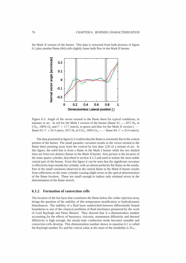
76 CHAPTER 6. BURNER CHARACTERIZATION
the Mark II version of the burner. This data is extracted fromboth pictures of figure6.1 plus another flame (#4) with slightly faster bulk flow in the Mark II burner.
-0.2
-0.1
0
0.1
0.2
0 0.2 0.4 0.6 0.8 1
Nor
mal
vec
tor
angl
e [a
rcm
inut
e]
Dimensionless Lateral position [ ]
-0.2
-0.1
0
0.1
0.2
0 0.2 0.4 0.6 0.8 1
Nor
mal
vec
tor
angl
e [a
rcm
inut
e]
Dimensionless Lateral position [ ]
-0.2
-0.1
0
0.1
0.2
0 0.2 0.4 0.6 0.8 1
Nor
mal
vec
tor
angl
e [a
rcm
inut
e]
Dimensionless Lateral position [ ]
Figure 6.3: Angle of the vector normal to the flame sheet for typical conditions, inminutes or arc. In red for the Mark I version of the burner (flame #1—, 30% H2 inCO2, 100% O2 andU � 17.7 mm/s), in green and blue for the Mark II version (- - -flame #3:U � 20.8 mm/s,30% H2 in CO2, 100% O2, – - –flame #4:U � 23.6 mm/s).
The data presented in figure 6.3 confirm that the flame is extremely flat in the centralportion of the burner. The small parasitic curvature results in the vector normal to theflame sheet pointing away from the vertical by less than1220 of a minute of arc. Inthis figure, the solid line is from a flame in the Mark I burner while the two dashedlines are from two distinct flames in the Mark II burner. Also picture is the location ofthe inner quartz cylinder, described in section 4.1.2 and used to isolate the most stablecentral part of the burner. From this figure it can be seen thatthe significant curvatureis effectively kept outside the cylinder, with an almost perfectly flat flame on the inside.Part of the small variations observed in the central flame in the Mark II burner resultsfrom reflections on the inner cylinder causing slight errorsin the optical determinationof the flame location. These are small enough to induce only minimal errors in thedetermination of the flame stretch.
6.1.2 Formation of convection cells
The location of the hot layer that constitutes the flame belowthe colder injection arraybrings the question of the stability of this temperature stratification to hydrodynamicdisturbances. The stability of a fluid layer sandwiched between differentially heatedboundaries is one of the classical problems of fluid mechanics pioneered by the workof Lord Rayleigh and Henri Benard. They showed that if a dimensionless numberaccounting for the effects of buoyancy, viscosity, momentum diffusivity and thermaldiffusivity is high enough, the steady-state conduction mode becomes unstable andconvection cells develop. This dimensionless number shownin equation 6.1 is calledthe Rayleigh numberRa and the critical value at the onset of the instability isRaC .

6.1. FLAME SHAPE 77
Ra � gBνDth
<T1 � T2A d3 � GrPr (6.1)
In this expression,g is the gravity acceleration,B the thermal expansion coefficient,ν the kinematic viscosity andDth the thermal diffusivity. The temperature difference isbetween the hot and cold boundaries, kept at temperaturesT1 andT2, respectively. Thelast parameter is the separation between the two boundariesd, which has a strong influ-ence and is included to the third power. The Rayleigh number can also be expressed bythe product of two other dimensionless numbers: the Grashofnumber and the Prandtlnumber. The Grashof number is the ratio of buoyancy and viscous forces while thePrandtl number accounts for the balance between thermal andmomentum diffusivities.Treatments of this problem in the literature abound, the interested reader is referred tothe classical book of Chandrasekhar [151] and the recent review of Bodenschatz et al.[152]. Variations on the classical configuration are also investigated with the introduc-tion of complications such as a Poiseuille flow parallel to the boundaries [153].
In the burner, the problem is further complicated by the bulkflow going through thesystem,perpendicularto the temperature gradient. Additionally, the two boundariesneed to be considered free because the flow is not restrained between the needles. Thisuncommon configuration has received little attention from theoreticians and experi-mentalists. A similar configuration exists industrially inthe porous media of fluidizedbed reactors which has received some attention [154] and theproblem has also beentreated analytically [155]. The most useful analysis foundin the literature, albeit on adifferent scale, was found in atmospheric sciences and focuses on convection inducedcloud formation. The extensive theoretical and experimental work of Krishnamurti[156, 157, 158] provides stability considerations including a large number of parame-ters.
The results of interest here is the influence of the bulk flow magnitude and directionon the stability of the layer. From the classical treatment of the problem it is knownthat the layer will be marginally stable for a criticalRac of approximately1708 if bothboundaries are rigid and657.5 if they are both free [151]. The effect of a bulk flowdirected from the hot to the cold boundary, such as in the burner used here, can have anopposite effect depending on the Prandtl number [156]. Small Prandtl numbers suchas those prevailing in the burner (on the order ofPr � 0.7), we can expect the criticalRayleigh number at which convection cells will develop todecreasewith increasingbulk velocity. This effect can be illustrated by considering the opposite case where ahigh Prandtl number results in thin thermal boundary layerson both sides of the domainconsidered. The addition of the bulk flow increases the boudary layers thickness andinduces a curvature in the conduction profile. As a result, although the temperaturegradient remains unchanged, it extends over a shorter depthand it follows an increasein the critical Rayleigh number.
When the flame position was lowered too far from the injectionarray, this resultedin the collapse of part of the flame and formation of stationary ridges in the reac-tion sheet, such as those shown in figure 6.4. Once the flame hadcollapsed, a stronghysteresis effect was observed, presumably from the heating of part of the injectionarray on either side of the burning chamber. The critical flame offsetd of 12 � 15
mm achievable while maintaining a planar flame results in a critical Rayleigh num-ber in qualitative agreement with the theoretical works mentioned above. Consideringthe uncertainties on the measured flame and injection array temperatures and the largenumber of parameters involved no further attempts were madetoward a quantitativecomparison.

78 CHAPTER 6. BURNER CHARACTERIZATION
�
�¡�����
Figure 6.4: Flame pattern observed when the flame position islow enough below theinjection array to result in the formation of convection cells in the burner.
6.2 Velocity measurements
6.2.1 Injection layer
The trick used to supply the counter-diffusing reactant to the burning chamber de-scribed in section 4.1.1 introduces localized inhomogeneities in the burning chamber.The introduction of hundreds of tiny jets in the bulk flow forms a thin region where thereactant intermixes with the flow of products. This region iscalled theinjection layerand must be measured to ensure that it does not perturb the flame. The main concern isthe determination of the thickness of this layer outside of which the transport of speciescan be considered strictly one-dimensional.
The only technique available with sufficient spatial resolution and the non-invasivecharacter required to probe the narrow jets produced by the injection needles is LaserDoppler Anemometry (LDA). The velocity was measured following the procedure de-scribed in section 4.3.1. Unfortunately, it was impossibleto seed the counter-diffusingspecies mixture with tracer particles since they tend to stick to the metal walls of thethin tubes of the injection arrays. Consequently, LDA measurements could only becarried out in the Mark I version of the burner where the bottom advected reactant isinserted through larger diameter tubes. The measurements were made without a flamepresent in the burner. When the burner is hot, the SiO2 seeding particles used becomepolarized from the pyroelectric effect and tend to stick to the burner windows abovethe flame. As a result, frequent shutdowns and cleanups are required, interrupting thelong acquisition times required to scan the region of interest.
Where the unseeded jets exiting the injection needles meet the seeded bulk flow,

6.2. VELOCITY MEASUREMENTS 79
the tracers are scarce and travel mostly vertically with thebulk flow. As a result, longintegration times where necessary to gather a usable signaland compressed air wasused in both streams to save pure gases. The transverse velocity profiles presented infigure 6.5 are taken at progressively greater depth below theinjection arrays. Onlythe vertical component of the velocity is plotted since the horizontal component ofthe LDA produced no usable signal from the small velocities along this axis and thelimited seeding issues mentioned above. The measurements of figure 6.5 show that thejets emanating from the needles have an effect on the bulk flowdown to between2.5
and3.0 mm below the injection array.
20
40
Position belowtube array
Ver
tica
l v
elo
city
[m
m/s
] -1.5 mm
15
25-2.0 mm
15
25-2.5 mm
15
25-3.0 mm
0.0 1.0 2.0 3.0 4.0
15
25
0.0 1.0 2.0 3.0 4.0
x [mm]
-3.5 mm
Figure 6.5: Velocity profiles taken at different depths below the injection array in theMark I version of the burner. The injection layer thickness is seen to be between2.5
and3.0 mm.
The value of2.5 mm is considered the upper bound for the the injection layer thick-ness since the typical bulk velocity in the burner when considering thermal expansionare higher that the value used for this experiment. Moreover, this value is the velocityinjection layer and the species concentration injection layer is likely to be smaller fromthe effect of diffusion. Below this layer, the flow can be considered one-dimensionalwith the transport of the species injected from the top beingdone only by diffusionagainst the bulk flow. All of the results presented in this thesis from this point onwardhave been gathered in this one-dimensional portion of the burner.
6.2.2 Transverse velocity profiles
The one-dimensional character of the flow throughout the burning chamber was veri-fied by taking velocity profiles across the entire burner cross section at different heights.These measurements were taken with a flame present in the burner and using LDAwhen possible. In the region of the burner where these measurements are carried

80 CHAPTER 6. BURNER CHARACTERIZATION
out, below the flame, the seeding is good and the temperature relatively low. Thismeans that more data points could be gathered before the windows became opaquefrom the accumulating seeding particles compared to the injection layer measurementspresented above. The velocity profile span almost the entirewidth of the burner butthe detailed measurements of the velocity boundary layers on the walls is prevented bylimited optical access.
Mark I burner
In the Mark I version of the burner, it was possible to use LDA as in section 6.2.1 toget two components of the velocity. The resulting velocity vectors taken across themidplane of the burner are presented in figure 6.6. The uppermost profile was taken inthe flame itself and each successive profile below it at increments of5 mm. From thisfigures it can be seen that the flow is not homogeneous at the bottom of the burner. Thisis attributed to the limited performance of the flow equalization chamber used on theadvected side of the Mark I burner. The imperative of lettingthe seeding particulatesgo through unimpeded prevented the use of a pressure drop sufficient to ensure uniformvelocity distribution.
-20
-15
-10
-5
0
0 5 10 15 20 25 30 35 40 45
Ver
tical
pos
ition
[mm
]
Lateral position [mm]
Figure 6.6: Vector plot of the velocity in the midplane of theMark I burner. Theuppermost profile is take in the flame itself.
As can be seen in the two uppermost profiles of figure 6.6, as theflow approachesthe flame it becomes significantly more homogeneous as it is accelerated followingthermal expansion. This can be more easily seen in figure 6.7,where each componentof the velocity was plotted separately. From these plots, the burning chamber belowthe flame can be separated in two regions. In the lower part of the burner the flow isconverging slightly towards the center of the burner but theopposite is observed whenapproaching the flame. From the horizontal component of the velocity it can be seenthat this phenomenon is more pronounced on the right side of the burner. Since it is onthat side that the ignition port is located, inducing higherheat losses, this converging-diverging flow can probably be attributed to thermal effectsat the windows.

6.2. VELOCITY MEASUREMENTS 81
0
10
20
30
40
50
60
70
0 5 10 15 20 25 30 35 40 45
Ver
tical
vel
ocity
[mm
/s]
Lateral position [mm]
0
10
20
30
40
50
60
70
0 5 10 15 20 25 30 35 40 45
Ver
tical
vel
ocity
[mm
/s]
Lateral position [mm]
0
10
20
30
40
50
60
70
0 5 10 15 20 25 30 35 40 45
Ver
tical
vel
ocity
[mm
/s]
Lateral position [mm]
0
10
20
30
40
50
60
70
0 5 10 15 20 25 30 35 40 45
Ver
tical
vel
ocity
[mm
/s]
Lateral position [mm]
(a)
-10
-5
0
5
10
0 5 10 15 20 25 30 35 40 45
Hor
izon
tal v
eloc
ity [m
m/s
]
Lateral position [mm]
-10
-5
0
5
10
0 5 10 15 20 25 30 35 40 45
Hor
izon
tal v
eloc
ity [m
m/s
]
Lateral position [mm]
-10
-5
0
5
10
0 5 10 15 20 25 30 35 40 45
Hor
izon
tal v
eloc
ity [m
m/s
]
Lateral position [mm]
-10
-5
0
5
10
0 5 10 15 20 25 30 35 40 45
Hor
izon
tal v
eloc
ity [m
m/s
]
Lateral position [mm]
(b)
Figure 6.7: The two components of the velocity in the Mark I burner plotted separately.The same profiles as in figure 6.6 are used, taken at different heights in the burner: atthe flame(2) and below the flame (5 mm (�), 10 mm (Q), 15 mm (�)). (a) Verticalcomponent. (b) Horizontal component.
Mark II burner
Using the thermistor-based system described in section 4.3.2 it was also possible toget some measurement of the velocity distribution in the Mark II version of the burner.However, since the probe used is not directional, only the absolute magnitude of thevelocity could be determined. This measurement could not berealized with a flamepresent in the burner, the thermistor having a maximum operating temperature of 250XC.Therefore, cold air was used to supply both streams. The profile shown in figure 6.8was taken at half the height of the burning chamber. The relatively large size of theprobe assembly used (about5 mm diameter) prevented the detailed measurements ofthe boundary layers on the chamber walls. Nevertheless, thefirst data points on eithersides of the profile still reveal the influence of the walls.
Comparing the Mark II profile of figure 6.8 to the ones taken at similar heightsin the Mark I burner presented in figure 6.7(a) reveal that thevelocity is much moreuniform in the new version of the burner. This difference is attributed partially to theabsence of a flame in these measurements but also to the improved injection plenumsused in the second version. The long plenums (80 mm) allowed the use of numerousdevices (screens, porous plates, honeycomb sections) to ensure homogeneous supplyto the injection needle array. The new plenum design and the needles themselves in-duced a pressure drop in the advected species injection pathsufficient to ensure a flatvelocity profile throughout the burning chamber. The previously mentioned drawbackof this approach is that the flow can no longer be seeded for LDA-based velocity mea-surements.
6.2.3 Residual strain
Transverse velocity profiles such as the uppermost one from figure 6.6 takeninsideastable flame typical of those encountered in this thesis allow the evaluation of the resid-ual stretch imposed on the flame. This quantity is of criticalimportance because of thestrong stabilizing effect it has on the thermal-diffusive instabilities. In the theoreticalmodels it is expected to be zero but experimentally there is no such thing and inhomo-

82 CHAPTER 6. BURNER CHARACTERIZATION
0
5
10
15
20
25
30
35
0 10 20 30 40 50 60 70
Vel
ocity
[mm
/s]
Lateral position [mm]
Figure 6.8: Transverse velocity profile in the Mark II version of the burner withouta flame present acquired using the hot thermistor technique.The Black vertical linesrepresent the position of the inner quartz tube walls. The horizontal dashed line is theaverage value expected from the supplied flow rate (28.41 mm/s).
geneity in the velocity distribution will induce a finite strain that must be quantified.The flame stretchK is a measure of rate of deformation of a surface element of theflame sheet of areaA as expressed by the following relation [159]:
K � 1
A
dA
dt(6.2)
Accordingly, a stretched flame has a positive value ofK while a compressed flameresults in a negativeK. The introduction of the concept is attributed to Karlovitzetal. [160] with the specific form of equation 6.2 depending on the geometric flameconfiguration. These authors investigated jet flames, wherethe reaction zone is locatedin a velocity gradient and found the the following form for the stretch rate:
K � 1
δ
1
U
dU
dy(6.3)
This expression for the stretch rate is known as the Karlovitz number whereU isthe velocity parallel to the flame sheet andy the coordinate normal to it. The parameterδ is a diffusion length defined asδ � λ2ρCpS
0f whereλ is the thermal conductivity,Cp
the specific heat andS0f the adiabatic flame speed. The Karlovitz number is sometimes
considered as a general definition of strain, but it is valid only in the specific configu-ration where it was developed. A general expression for flamestretch was derived byMatalon [161, 162] and is presented in equation 6.4. This formulation was selectedbecause it is dependent upon physically measurable quantities, is independent on theflame configuration and the choice of coordinate system.
K � Vf� � n � ~n � � � <~v � ~nA (6.4)
Equation 6.4 was developed for the case of premixed combustion withVf the flamesheet propagation speed projected on its normal vector~n and~v the velocity vector. In

6.3. TEMPERATURE MEASUREMENTS 83
diffusion flames, the reaction front does not propagate and the stretch equation usedmust be modified by settingVf � 0. What remains is only the second term of equation6.4, that can be expanded using the triple product rule in thefollowing way:
K � �~n � � � <~v � ~nAK � �~n �~v<� � ~nA � ~n<� � ~vA � <~n � �A~v � <~v � �A~n�K � �<~n � ~vA<� � ~nA � ~n � <1
2<�~v � <�~vAT AA � ~n
K � �<~n � ~vA<� � ~nA � ~n �E � ~n � Kc � Ks (6.5)
In this last equation,E represents the rate of strain tensor [163, 162]. The firstterm isolated in equation 6.5 represents a contribution of the flame curvature to theflame stretch that was hidden in the second term of equation 6.4. The second termof equation 6.5 is the change in flame surface area induced by the strain in the flow.The total stretch experiences by the flame is therefore the superposition of the stretchcontributions induced by the flame front curvature (Kc) and by the flow strain (Ks),even in the absence of flame propagation.
Using this formula, a velocity profile taken in the flame frontsuch as the one pre-sented in figure 6.9(a) and the flame shape extracted from figure 6.1 it is possible toquantify flame stretch. The result is presented in figure 6.9(b) with total stretch andthe separate contributions of curvature and strain plottedseparately. As expected, theresidual stretch is extremely low, below0.15 s�1 everywhere in the burner. It shouldbe noted that these results are from the Mark I burner since only in this version LDAcould be used to gather the velocity vector field. From the data presented in figure 6.3it is reasonable to expect that the maximum stretch in the Mark II version of the burnershould be of the same order of magnitude. In this version, thecentral portion of theburner were measurements are conducted is shielded from theslightly stretched flameedges by the quartz cylinder. In the corresponding region ofthe Mark I burner, thestretch is below0.05 s�1 and this value is expected in the center of the quartz cylinderin the Mark II version. However, it is necessary to remember that this inner quartzcylinder will induce a velocity boundary layer in the inner flame, which will cause itsedges to be slightly more stretched than its center. However, without LDA velocitymeasurements, the magnitude of this stretch is impossible to quantify more preciselythan the values given above.
6.3 Temperature measurements
The flame temperature was measured using thermocouples following the proceduredescribed in section 4.4. A picture presenting two probes inthe burner with a stablehydrogen flame present is shown in figure 6.10. The triangularshape of the probes waschosen to minimize the conduction losses of the thermocouple junction by placing thejunction wires parallel to the temperature gradient. Because of this design choice, thetemperature measurements could not be done with the inner quartz cylinder present inthe burner. The measurements were done in the Mark II versionof the burner with thesize of the probes necessitating the use of the longer burning chamber length setting of40 mm. The parameters used are typical for the stable flames presented in this chapterand are listed under flame #2 in table 6.1.
Great efforts were taken to mitigate the effects of catalytic heating and radiationlosses of the thermocouple junction, as described in section 4.4. The effect of the coat-
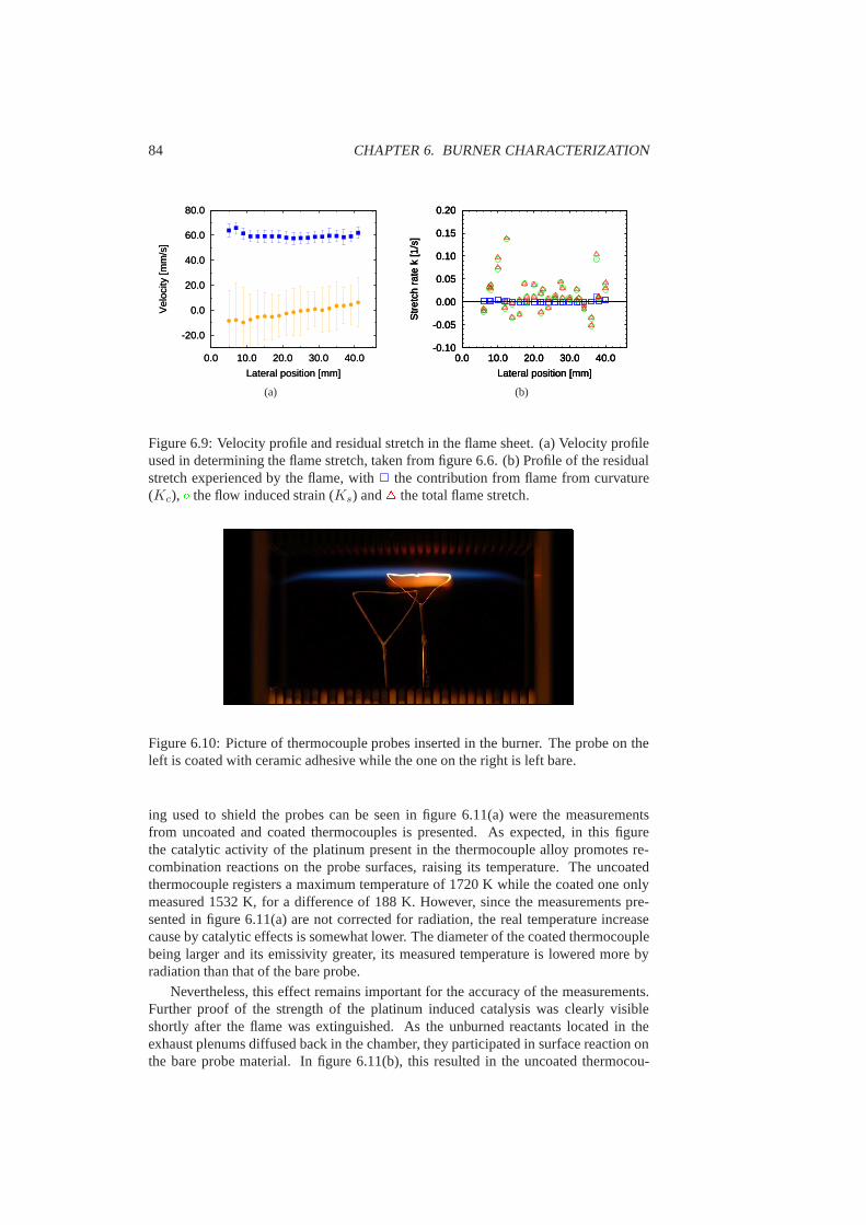
84 CHAPTER 6. BURNER CHARACTERIZATION
-20.0
0.0
20.0
40.0
60.0
80.0
0.0 10.0 20.0 30.0 40.0
Vel
ocity
[mm
/s]
Lateral position [mm]
-20.0
0.0
20.0
40.0
60.0
80.0
0.0 10.0 20.0 30.0 40.0
Vel
ocity
[mm
/s]
Lateral position [mm]
(a)
-0.10
-0.05
0.00
0.05
0.10
0.15
0.20
0.0 10.0 20.0 30.0 40.0
Str
etch
rat
e k
[1/s
]
Lateral position [mm]
-0.10
-0.05
0.00
0.05
0.10
0.15
0.20
0.0 10.0 20.0 30.0 40.0
Str
etch
rat
e k
[1/s
]
Lateral position [mm]
-0.10
-0.05
0.00
0.05
0.10
0.15
0.20
0.0 10.0 20.0 30.0 40.0
Str
etch
rat
e k
[1/s
]
Lateral position [mm]
(b)
Figure 6.9: Velocity profile and residual stretch in the flamesheet. (a) Velocity profileused in determining the flame stretch, taken from figure 6.6. (b) Profile of the residualstretch experienced by the flame, with2 the contribution from flame from curvature(Kc), X the flow induced strain (Ks) andQ the total flame stretch.
Figure 6.10: Picture of thermocouple probes inserted in theburner. The probe on theleft is coated with ceramic adhesive while the one on the right is left bare.
ing used to shield the probes can be seen in figure 6.11(a) werethe measurementsfrom uncoated and coated thermocouples is presented. As expected, in this figurethe catalytic activity of the platinum present in the thermocouple alloy promotes re-combination reactions on the probe surfaces, raising its temperature. The uncoatedthermocouple registers a maximum temperature of 1720 K while the coated one onlymeasured 1532 K, for a difference of 188 K. However, since themeasurements pre-sented in figure 6.11(a) are not corrected for radiation, thereal temperature increasecause by catalytic effects is somewhat lower. The diameter of the coated thermocouplebeing larger and its emissivity greater, its measured temperature is lowered more byradiation than that of the bare probe.
Nevertheless, this effect remains important for the accuracy of the measurements.Further proof of the strength of the platinum induced catalysis was clearly visibleshortly after the flame was extinguished. As the unburned reactants located in theexhaust plenums diffused back in the chamber, they participated in surface reaction onthe bare probe material. In figure 6.11(b), this resulted in the uncoated thermocou-

6.3. TEMPERATURE MEASUREMENTS 85
ple becoming incandescent from the surface reactions, witha measured temperature of1400XC without a flame in the burner. The phenomenon lasted from 5 to10 minutesafter the flame was extinguished and was sufficient to reignite the flame if the flow ofgases was restored.
0
250
500
750
1000
1250
1500
1750
2000
0 0.1 0.2 0.3 0.4 0.5 0.6 0.7 0.8 0.9 1
Tem
pera
ture
[K]
Dimensionless position [ ]
U
0
250
500
750
1000
1250
1500
1750
2000
0 0.1 0.2 0.3 0.4 0.5 0.6 0.7 0.8 0.9 1
Tem
pera
ture
[K]
Dimensionless position [ ]
U
(a) (b)
Figure 6.11: (a) Longitudinal temperature profiles from coated (2) and uncoated (X)probes (flame #2). (b) Catalytic effect on platinum wire resulting in incandescent wireeven in the absence of a flame.
The measurements were corrected for radiation following the procedure describedin section 4.4.3 with values of the emissivities used for theradiation correction given inthat section. The magnitude of the radiation correction as afunction of the temperature,for a coated probe, is given in figure 6.12. For the measurements of the maximumflame temperature, the radiation correction reaches about 350 K. In this figure, the twodatasets illustrates the effect of neglecting the radiation received by the probe fromthe enclosure walls. This simplification results in an overestimation of the radiationcorrection of 25 K relative to the assumption of a representative wall temperature of500 K. For the results presented from this point onward, the radiation received fromthe walls will be included in the calculation of the radiation correction.
The radiation corrected data for the uncoated and coated probes is presented infigures 6.13(a) and 6.13(b), respectively. In these figures,the solid black line representsthe temperature profile obtained from the numerical model described in section 3.3.The radiation correction resulted in the difference between the coated and uncoatedprobes to decrease from 188 K to 150 K. This difference can be entirely attributed tothe catalytic effects on the probe surface and is sufficient for the uncoated thermocouplemeasurement to clearly overestimate the flame temperature.
The radiation-corrected data from the coated thermocouplemeasurement is com-pared in figure 6.14 to both the numerical results and the prediction of the simplifiedmodel presented in section 3.1.2, with the three datasets showing remarkable agree-ment, within50 K. The maximum flame temperature reached in the theoretical profilewas determined following the procedure described in section 3.1.3. The small differ-ence in the experimental data on the cold advected side of theburner can simply beexplained by the boundary conditions used for the theoretical and numerical models.The value of 500 K used in the models is representative of a large range of flames whilethe specific experimental data plotted in this figure has an injection temperature at theadvected end of 460 K.

86 CHAPTER 6. BURNER CHARACTERIZATION
-50
0
50
100
150
200
250
300
350
400
0 200 400 600 800 1000 1200 1400 1600
Tem
pera
ture
cor
rect
ion
[K]
Dimensionless position [ ]
-50
0
50
100
150
200
250
300
350
400
0 200 400 600 800 1000 1200 1400 1600
Tem
pera
ture
cor
rect
ion
[K]
Dimensionless position [ ]
Figure 6.12: Magnitude of the radiation correction for a coated probe as a function ofmeasured temperature, by neglecting the radiation received by the probe from the walls(X) and by assuming a representative wall temperature of500 XC (2).
6.3.1 Temperature in the burning chamber
From the shape of the flame presented in figure 6.1, it seems obvious that the flameintensity and therefore its temperature is not uniform overthe burner cross section.To measure this temperature variation, a coated thermocouple probe was successivelyintroduced in the burning chamber through different extraction tubes. The resultingtransverse temperature profile is presented in figure 6.15. The effect of the walls in-duces a significant reduction of the flame temperature on the periphery of the burningchamber, in excess of 350 K. In this figure, the solid and dashed lines represent theadiabatic flame temperature and the result of the numerical model, respectively.
The use of the quartz cylinder described in section 4.1.2 allows the inner flamewhere the measurements are conducted to be much closer to isothermal. The positionof the cylinder is illustrated in the figure by the vertical lines. Within this region,the flame temperature deviates no more than 125 K from either the adiabatic flametemperature or the flame temperature obtained numerically.Heat loss only account forpart of the deviation since, as will be discussed in the next section, inhomogeneities inthe species distribution results in a reduced mixture strength on the burner edges.
6.4 Species measurements
The measurement of mixture composition in the burning chamber was done using massspectrometry, with the equipments and procedures described in chapter 5. This tech-nique was employed throughout this thesis to establish the effective boundary condi-tions at the counter-diffusing inlet of the burner. It was also used to characterize thespecies distribution in the burner and the flames generated.These results are presentedin this section.

6.4. SPECIES MEASUREMENTS 87
0
250
500
750
1000
1250
1500
1750
2000
0 0.1 0.2 0.3 0.4 0.5 0.6 0.7 0.8 0.9 1
Tem
pera
ture
[K]
Dimensionless position [ ]
U
0
250
500
750
1000
1250
1500
1750
2000
0 0.1 0.2 0.3 0.4 0.5 0.6 0.7 0.8 0.9 1
Tem
pera
ture
[K]
Dimensionless position [ ]
U
0
250
500
750
1000
1250
1500
1750
2000
0 0.1 0.2 0.3 0.4 0.5 0.6 0.7 0.8 0.9 1
Tem
pera
ture
[K]
Dimensionless position [ ]
U
(a)
0
250
500
750
1000
1250
1500
1750
2000
0 0.1 0.2 0.3 0.4 0.5 0.6 0.7 0.8 0.9 1
Tem
pera
ture
[K]
Dimensionless position [ ]
U
0
250
500
750
1000
1250
1500
1750
2000
0 0.1 0.2 0.3 0.4 0.5 0.6 0.7 0.8 0.9 1
Tem
pera
ture
[K]
Dimensionless position [ ]
U
0
250
500
750
1000
1250
1500
1750
2000
0 0.1 0.2 0.3 0.4 0.5 0.6 0.7 0.8 0.9 1
Tem
pera
ture
[K]
Dimensionless position [ ]
U
(b)
Figure 6.13: Radiation corrected longitudinal temperature profiles (X) and untreatedmeasured temperatures (2). a) Using uncoated thermocouple probes; b) Using coatedthermocouple probe. The solid black line is the profile obtained from the numericalmodel. The catalytic effects on the uncoated thermocouple surface result in an overes-timation of the flame temperature.
0
250
500
750
1000
1250
1500
1750
2000
0 0.1 0.2 0.3 0.4 0.5 0.6 0.7 0.8 0.9 1
Tem
pera
ture
[K]
Dimensionless position [ ]
U
0
250
500
750
1000
1250
1500
1750
2000
0 0.1 0.2 0.3 0.4 0.5 0.6 0.7 0.8 0.9 1
Tem
pera
ture
[K]
Dimensionless position [ ]
U
0
250
500
750
1000
1250
1500
1750
2000
0 0.1 0.2 0.3 0.4 0.5 0.6 0.7 0.8 0.9 1
Tem
pera
ture
[K]
Dimensionless position [ ]
U
Figure 6.14: Comparison between experimental (X), numerical (—) and theoretical (–– –) longitudinal temperature profiles. The experimental values are slightly shifted tothe left as a result of the small conduction losses in the probe assembly.
6.4.1 Species transverse concentration profiles
In the previous two sections it was shown that the temperature and velocity boundarylayers in the burning chamber and chimney are significant issues in the burner design

88 CHAPTER 6. BURNER CHARACTERIZATION
0
500
1000
1500
2000
0 10 20 30 40 50 60 70
Fla
me
Tem
pera
ture
[K]
Lateral Position [mm]
0
500
1000
1500
2000
0 10 20 30 40 50 60 70
Fla
me
Tem
pera
ture
[K]
Lateral Position [mm]
0
500
1000
1500
2000
0 10 20 30 40 50 60 70
Fla
me
Tem
pera
ture
[K]
Lateral Position [mm]
Figure 6.15: Flame temperature distribution across the burning chamber. The verticallines represent the position of the walls of the inner quartzcylinder. The measure-ments were made with coated thermocouples,� uncorrected temperatures,X radiationcorrected temperatures. The solid and dashed lines represent the adiabatic flame tem-perature and the result of the numerical model, respectively.
used here. From these findings is appears obvious that the injection layer would besubjected to slightly different conditions across the injection array. By introducing themass spectrometer capillary through successive extraction needles, it was possible tocharacterize the species distribution in the injection layer and the define the variationof the boundary conditions at the counter-diffusing end. The results presented in figure6.16(a) and 6.16(b), covering one half of the burner cross section, show the variationof the oxidant volume fraction and the corresponding changein mixture strength, re-spectively. Once again, the vertical lines represent the position of the inner quartzcylinder. Within this inner region of the flame, the mixturesstrength was measured tobe uniform within 10% of its average values. On the edges of the burning chamber, thephenomena listed above result in the flame having a mixture strength over 50% lower.This considerably leaner periphery flames is colder and reaches instability well beforethe central region, often becoming extinct as the instabilities are still studied within thequartz cylinder.
This variation in the mixture strengthφ measured in figure 6.16(b) is believed tobe the main cause of the rapid cell motion observed in the cellular flames developingin the Mark I version of the burner, shown in figure 4.3. Ratherthan being causedby heat loss at the chamber windows, as was initially believed, the heat loss in thechimney is expected to play a central role in the phenomenon.The walls of the chimneybeing colder, the exit velocity of the species injected through the needles is higherin the periphery rows of the array. Additionally, the upwardvelocity is slower therebecause of the boundary layer developing in the burning chamber. The result from thecombination of these effects is a higher concentration of the counter-diffusive speciesclose to the chamber walls. Thisφ variation induces flame curvature and associatedflame stretch that is responsible for the cell motion.
The introduction of the inner quartz cylinder in the burningchamber, as describedin section 4.1.2 only addresses one of these problems, sincevelocity boundary lay-ers are still present within the cylinder. However, the goodflame flatness (see section6.1) and absence of cell motion (see section 7.3) observed within the cylinder revealthat the influence of the velocity boundary layer is small. Solving the problem of thecurvature of the flame edges and residual stretch would require the homogenization

6.4. SPECIES MEASUREMENTS 89
0
0.1
0.2
0.3
0.4
0.5
0 5 10 15 20 25 30 35
O2
vol.
frac
tion
[ ]
Lateral Position [mm]
(a)
0
0.1
0.2
0.3
0.4
0.5
0.6
0.7
0 5 10 15 20 25 30 35
Mix
ture
str
engt
h [ ]
Lateral Position [mm]
(b)
Figure 6.16: Effect of the walls on the oxidant distributionin the chamber, over one halfof the burner cross section. (a) Variation of the O2 volume fraction. (b) Correspondingchange in the mixture strength. The vertical lines represent the position of the innerquartz cylinder.
of the temperature distribution in the burner chimney. Placing the whole assembly inan oven set at a temperature close to that of the exhaust wouldhelp but complicateoptical access to the burning chamber. Localized heating onthe chimney is anotheroption but would require the presence of a heat conductive fluid, perhaps circulated,in the space between the injection and extraction arrays to ensure sufficient heat trans-fer. Some experimentations were made following this concept, with the very limitedbeneficial effect not outweighing the considerable increase in system complexity. Inthe end, since improvements provided by simply using a quartz cylinder to isolate theunstretched central region of the burner proved sufficient to allow the observation ofstationary cellular flames, only this solution was implemented. This choice explainsthe significant increase in the area of the burner cross-section between the Mark I andthe Mark II, to ensure that the inner unstretched region was large enough to conductmeaningful experiments.
6.4.2 Species longitudinal concentration profiles
Species concentration profiles covering the length of the burning chamber were alsoobtained by slowly moving the tip of the mass spectrometer capillary from the outsidewith a stable flame burning in the chamber. The procedure is described in chapter 5 and

90 CHAPTER 6. BURNER CHARACTERIZATION
is only able to measure stable species, with an estimated relative accuracy of about 5%for most of the mixtures measured. Close to the flame sheet, the large concentration ofradical species can results in additional errors of up to 10%.
The profiles presented in figure 6.17(a) and 6.17(b) cover thecases where the fuelis advected and counter-diffusing, respectively. The concentration of the fuel (H2), ox-idant (O2) and product (H2O) are included. The profiles expected from the simplifiedtheoretical model presented in section 3.1 are also plottedusing solid lines. There isa surprisingly good agreement between the experiment and the simplified model, con-sidering the drastic assumptions that were made in developing it, especially regardingthe constant transport properties. These being evaluated at the flame temperature, itis without surprise that the main disagreement between the two are found in the coldregion close to the advected species inlet.
The results obtained from the numerical model are also plotted in figure 6.17(a),using dashed lines. The agreement with the experimental data on the side where the fuelis advected is not very good, which is surprising considering that the model accounts forthe variation of the transport properties with temperature. However, as seen previously,the model properly accounts for the flame position and the temperature profile. In thefuel counter-diffusing configuration, the numerical modelfailed to converge to a stableburning state. The reason for these errors is unknown, but since the numerical treatmentof the problem is not the main concern of this thesis, this topic was not investigatedfurther.
6.5 Flame position
To measure the flame location in the burner, photographs where taken from the side,following the procedure described in section 4.2.1. The images where then analyzedand the flame position determined as the point of maximum luminosity in the center ofthe chamber. This optically determined flame location was verified to be in excellentagreement with the location of the water concentration and temperature maxima. Forthe sake of simplicity, the optical method was used for all ofthe results presented here.
6.5.1 Virtual origin
The procedure used to determine the boundary condition at the counter-diffusing endof the burner is illustrated in figure 6.18. For each experimental condition, the mix-ture composition immediately next to the injection needle array supplying the counter-diffusing species was measured by mass spectrometry. Theselocal concentration pro-files (shown in the insert of figure 6.18, about5 to 10 mm long), extending from theinjection tube tips to the flame, allowed the determination of the amount of counter-diffusing reactant swept into the exhaust by the bulk flow, and hence the effective mix-ture strength in the burner. Based on this concentration profile, a point beyond theinjection layer was chosen as thevirtual origin of the counter-diffusing reactant.
The use of this short profile instead of a single point allowedsome latitude in choos-ing the reference point to generate large datasets with moreor less constant mixturestrength. For instance, when increasing the bulk velocity the injection layer thicknessdecreased even if all other parameters remains constant. Accordingly, the oxygen con-centration at a reference point3.5 mm below the array decreased. This resulted in themixture strength measured at that reference point to increase. To be able to use thesetwo data points to measure the influence of bulk velocity on flame position, a new

6.5. FLAME POSITION 91
0
0.25
0.5
0.75
1
0 0.2 0.4 0.6 0.8 1 0
0.25
0.5
0.75
1
Fue
l mas
s fr
actio
n [ ]
Oxi
dant
mas
s fr
actio
n [ ]
Dimensionless position [ ]
U
0
0.25
0.5
0.75
1
0 0.2 0.4 0.6 0.8 1 0
0.25
0.5
0.75
1
Fue
l mas
s fr
actio
n [ ]
Oxi
dant
mas
s fr
actio
n [ ]
Dimensionless position [ ]
U
0
0.25
0.5
0.75
1
0 0.2 0.4 0.6 0.8 1 0
0.25
0.5
0.75
1
Fue
l mas
s fr
actio
n [ ]
Oxi
dant
mas
s fr
actio
n [ ]
Dimensionless position [ ]
U
0
0.25
0.5
0.75
1
0 0.2 0.4 0.6 0.8 1 0
0.25
0.5
0.75
1
Fue
l mas
s fr
actio
n [ ]
Oxi
dant
mas
s fr
actio
n [ ]
Dimensionless position [ ]
U
0
0.25
0.5
0.75
1
0 0.2 0.4 0.6 0.8 1 0
0.25
0.5
0.75
1
Fue
l mas
s fr
actio
n [ ]
Oxi
dant
mas
s fr
actio
n [ ]
Dimensionless position [ ]
U
0
0.25
0.5
0.75
1
0 0.2 0.4 0.6 0.8 1 0
0.25
0.5
0.75
1
Fue
l mas
s fr
actio
n [ ]
Oxi
dant
mas
s fr
actio
n [ ]
Dimensionless position [ ]
U
0
0.25
0.5
0.75
1
0 0.2 0.4 0.6 0.8 1 0
0.25
0.5
0.75
1
Fue
l mas
s fr
actio
n [ ]
Oxi
dant
mas
s fr
actio
n [ ]
Dimensionless position [ ]
U
(a) Fuel advected
0
0.5
1
1.5
2
0 0.2 0.4 0.6 0.8 1 0
0.5
1
1.5
2
Fue
l mas
s fr
actio
n [ ]
Oxi
dant
mas
s fr
actio
n [ ]
Dimensionless position [ ]
U
0
0.5
1
1.5
2
0 0.2 0.4 0.6 0.8 1 0
0.5
1
1.5
2
Fue
l mas
s fr
actio
n [ ]
Oxi
dant
mas
s fr
actio
n [ ]
Dimensionless position [ ]
U
0
0.5
1
1.5
2
0 0.2 0.4 0.6 0.8 1 0
0.5
1
1.5
2
Fue
l mas
s fr
actio
n [ ]
Oxi
dant
mas
s fr
actio
n [ ]
Dimensionless position [ ]
U
0
0.5
1
1.5
2
0 0.2 0.4 0.6 0.8 1 0
0.5
1
1.5
2
Fue
l mas
s fr
actio
n [ ]
Oxi
dant
mas
s fr
actio
n [ ]
Dimensionless position [ ]
U
0
0.5
1
1.5
2
0 0.2 0.4 0.6 0.8 1 0
0.5
1
1.5
2
Fue
l mas
s fr
actio
n [ ]
Oxi
dant
mas
s fr
actio
n [ ]
Dimensionless position [ ]
U
(b) Fuel counter-diffusing
Figure 6.17: Longitudinal species concentration profiles,fuel (�), oxidant (�) andwater (X). The solid and dashed lines are the profiles obtained from the simplifiedtheory and numerical models, respectively.
��������
����
�¡�����
�����������¢��
� ��� �¡�� ¡���
¡��� ¡�����
¡�����
�� �� �������¢ ������� �������¢����
Figure 6.18: Sketch illustrating the technique used to set the virtual origin of the sys-tem. The short profile of counter-diffusing species concentration taken below the in-jection array (shown in the insert) allow the choice of reference points with the samemixture strength despite different injection layers.
reference point was chosen slightly downstream from the first one, where the oxidant

92 CHAPTER 6. BURNER CHARACTERIZATION
concentration was the same as in the first case. The result is that for the two data pointsthe chamber length is slightly different and this was accounted for in the normalizationprocess.
In the measurements presented here, the change in the virtual position associatedwith a change in bulk flow velocity was relatively small, on the order of1 to 2 mmat the maximum. The minimum distance between the virtual origin and the needlearray was always chosen to ensure that the reference point was outside of the injectionlayer. Following the measurements presented in section 6.2.1, this distance was set at2.5 mm. The use of a two gas mixture (helium and CO2) allowed the investigationof the effect of the Lewis number on flame position. Change in the inert compositionand therefore in the advected mixture density, caused an effect of larger magnitude onthe mixture strength than the one described previously for the bulk velocity. As can beseen in figure 6.19, when the inert gas was progressively changed from pure CO2 topure He at constant bulk velocity, the virtual origin had to be changed by about3 to 7
mm to maintain a constant mixture strength.
0.050.10
0.150.20
0.250.30
0.35 15.020.0
25.030.0
0
1
2
3
4
5
6
7
Virt
ual o
rigin
[mm
]
Density [kg/m3] Bulk velocity [mm/s]
0.050.10
0.150.20
0.250.30
0.35 15.020.0
25.030.0
0
1
2
3
4
5
6
7
Virt
ual o
rigin
[mm
]
Density [kg/m3] Bulk velocity [mm/s]
0.050.10
0.150.20
0.250.30
0.35 15.020.0
25.030.0
0
1
2
3
4
5
6
7
Virt
ual o
rigin
[mm
]
Density [kg/m3] Bulk velocity [mm/s]
0.050.10
0.150.20
0.250.30
0.35 15.020.0
25.030.0
0
1
2
3
4
5
6
7
Virt
ual o
rigin
[mm
]
Density [kg/m3] Bulk velocity [mm/s]
Figure 6.19: Effect of bulk velocity and mixture density on the virtual origin used toachieve a constant mixture strength ofφ � 0.5.
The displacement of the virtual origin proved a suitable technique to account forboth of the effect of the bulk velocity and advected mixture density on the effectivemixture strength. The mixture composition and temperatureat the reference point werethen used as boundary condition and the reduced chamber length as the new referencelength for the comparison with the simplified model of section 3.1. This procedureallowed the effective mixture strengthφ to be kept constant, despite the varying lossof counter-diffusing species into the exhaust at differentbulk flow velocities and in-ert composition. To evaluate the theoretical flame position, the experimental Lewisnumbers of the reactants were evaluated using the mixture composition and tempera-ture measured at the flame. The dimensional bulk velocity wasdetermined from thesupplied mass flow rate.

6.5. FLAME POSITION 93
6.5.2 Influence of bulk velocity
The position of the flame inside the burning chamber as a function of the bulk velocitymagnitude and direction was investigated using CO2 diluted H2-O2 flames. The re-sults are presented in figure 6.20(a) and 6.20(b) for the fueladvected and fuel counter-diffusing configurations, respectively. Because of the limits imposed by the counter-diffusing species injection scheme, it was impossible to obtain data with the same mix-ture strength for both the fuel advected and fuel counter-diffusingconfigurations. Whenthe fuel is counter-diffusing, most of it is carried away in the exhaust by the compara-tively heavier inert. Accordingly, the flames produced in this configuration are alwaysvery lean. Typical results are presented in figure 6.20(b) for φ � 0.33 andφ � 0.25.
The thermal diffusivityDth, used to determine the dimensionless bulk velocity wasevaluated at three different temperatures for comparison purposes: at both inlet tem-peratures and at the flame temperature measured or as determined either numericallyor using the method described in section 3.1.3. The result presented in figure 6.20clearly show that the flame temperature is the most appropriate to evaluateDth usedin the dimensionless bulk velocity. When this reference point is used, the results showgood agreement between the simplified theory for the flame position (equation 3.14)and the experimental results. The figures also show that the flame position is more ac-curately predicted by the simplified theory when the oxygen rather than the hydrogenis counter-diffusing.
Several factors can be invoked to explain the differences between the two data sets.The assumption of constant transport properties made in thetheoretical developmentis not equally drastic in both configurations. Equation (3.14) reveals that the flame po-sition is mainly determined by the Lewis number of the counter-diffusing species. Inthis dataset,Leo varied only slightly from the injection point to the flame sheet (from0.861 to 0.865) when the oxidant was counter diffusing. Whenthe fuel was counter-diffusing, theLef variation was more significant, between 0.25 at the injection and0.22 at the flame, on average. In addition, the thermal expansion, also neglected in thesimplified theory, decreases the transport of the counter-diffusing species to the reac-tion zone. This effect increases the effectiveφ when the oxidant is counter-diffusingand decreases it in the reverse configuration (note that a decreasingφ lowers the curvexf <UA in figures 6.20(a) and 6.20(b)).
6.5.3 Influence of Lewis number
From the simplified theory described in section 3.1, when thevelocity is high, only theLewis number of the counter-diffusing species is expected to have a significant effecton flame position. However, when the velocity is small, both Lewis number need to beconsidered because the forward diffusion of the advected species becomes significant.To test this theory, the reactants were diluted in a mixture of two inerts (helium andCO2) to generate a range of Lewis numbers for the two reactants. In these results thefuel-advected configuration was used and accordingly the Lewis number of the oxidant(Leo) is expected to have a dominating influence on the flame position. Assuming aconstant Lef , the expected flame position dependence on Leo and U is given in figure6.21(a).
The use of helium as a dilution gas with its high thermal diffusivity means that thedimensionless velocity is relatively small, so the Lewis number of the advected specieshas to be taken into account. In figure 6.21(b), the flame position predicted by thetheory is showed with and without considering the variationin the advected species

94 CHAPTER 6. BURNER CHARACTERIZATION
0
0.2
0.4
0.6
0.8
1
-20 -10 0 10 20 30 40
x f [
]
Dimensionless velocity U [ ]
0
0.2
0.4
0.6
0.8
1
-20 -10 0 10 20 30 40
x f [
]
Dimensionless velocity U [ ]
0
0.2
0.4
0.6
0.8
1
-20 -10 0 10 20 30 40
x f [
]
Dimensionless velocity U [ ]
0
0.2
0.4
0.6
0.8
1
-20 -10 0 10 20 30 40
x f [
]
Dimensionless velocity U [ ]
(a)
0
0.2
0.4
0.6
0.8
1
-20 -15 -10 -5 0 5 10
x f [
]
Dimensionless velocity U [ ]
0
0.2
0.4
0.6
0.8
1
-20 -15 -10 -5 0 5 10
x f [
]
Dimensionless velocity U [ ]
0
0.2
0.4
0.6
0.8
1
-20 -15 -10 -5 0 5 10
x f [
]
Dimensionless velocity U [ ]
0
0.2
0.4
0.6
0.8
1
-20 -15 -10 -5 0 5 10
x f [
]
Dimensionless velocity U [ ]
0
0.2
0.4
0.6
0.8
1
-20 -15 -10 -5 0 5 10
x f [
]
Dimensionless velocity U [ ]
0
0.2
0.4
0.6
0.8
1
-20 -15 -10 -5 0 5 10
x f [
]
Dimensionless velocity U [ ]
0
0.2
0.4
0.6
0.8
1
-20 -15 -10 -5 0 5 10
x f [
]
Dimensionless velocity U [ ]
0
0.2
0.4
0.6
0.8
1
-20 -15 -10 -5 0 5 10
x f [
]
Dimensionless velocity U [ ]
(b)
Figure 6.20: Effect of bulk flow velocity on flame position forthe case ofcounter-diffusing oxidant (a) and counter-diffusing fuel(b). TheDth used to non-dimensionalize the bulk velocity is evaluated at the flame (2), at the advecting inlet (X)and at the counter-diffusing inlet (Q). The lines represent the flame position predictedby the simplified theory, a) ——, forφ � 1, Lef � 0.35 andLeo � 0.85, b)Lef � 0.25,Leo � 0.80, φ � 0.25 (filled symbols and solid line) andφ � 0.33 (open symbols anddashed theoretical line).
Lewis number. For the low-velocity flames considered here (0.4 1 U 1 2), neglectingthe advected species Lewis number results in differences ofup to 12% in the predicteddimensionless flame position.
0.2 0.3 0.4 0.5 0.6 0.7 0.8 0.9
0.751.00
1.251.50
1.75-4.0
-2.00.0
2.04.0
0
0.2
0.4
0.6
0.8
1
Fla
me
posi
tion
[ ]
Oxidant Lewis number Bulk velocity [ ]
0.2 0.3 0.4 0.5 0.6 0.7 0.8 0.9
0.751.00
1.251.50
1.75-4.0
-2.00.0
2.04.0
0
0.2
0.4
0.6
0.8
1
Fla
me
posi
tion
[ ]
Oxidant Lewis number Bulk velocity [ ]
0.2 0.3 0.4 0.5 0.6 0.7 0.8 0.9
0.751.00
1.251.50
1.75-4.0
-2.00.0
2.04.0
0
0.2
0.4
0.6
0.8
1
Fla
me
posi
tion
[ ]
Oxidant Lewis number Bulk velocity [ ]
(a)
0.751.00
1.251.50
1.75-4.0
-2.00.0
2.04.0
0
0.2
0.4
0.6
0.8
1
Fla
me
posi
tion
[ ]
Oxidant Lewis number Bulk velocity [ ]
0.751.00
1.251.50
1.75-4.0
-2.00.0
2.04.0
0
0.2
0.4
0.6
0.8
1
Fla
me
posi
tion
[ ]
Oxidant Lewis number Bulk velocity [ ]
0.751.00
1.251.50
1.75-4.0
-2.00.0
2.04.0
0
0.2
0.4
0.6
0.8
1
Fla
me
posi
tion
[ ]
Oxidant Lewis number Bulk velocity [ ]
(b)
Figure 6.21: Effect of bulk velocity and counter-diffusingspecies Lewis number (Leo)on flame position predicted by the simplified theory. a) The fuel Lewis number isassumed constant and the mixture strength isφ � 0.5. b) Theoretical results, with (X)and without (2) considering the variation of Lef measured for the experimental datapoints available.
The results gathered in these conditions and presented in figure 6.22 confirm thenecessity of considering both Lewis numbers. In figure 6.22(a), the measured flame po-sition from the virtual origin is simply normalized using the reduced chamber length1.A comparison between these results and the theoretically predicted values, even con-sidering the variation of both Lewis numbers, yields considerable errors. For the data
1The reduced chamber length is the total chamber length minusthe position of the virtual origin used.

6.5. FLAME POSITION 95
presented in figure 6.22(a), the error exceeds 20% for the flames with the lowest bulkflows.
This discrepancy can be explained by considering that for the low velocities usedfor this experiment, the conditions present at the end of thebottom injection tubes arenot the same as in the prescribed gas stream. With the small chamber length2 usedhere (20 mm), the bottom injection array is located in a region with significant concen-tration gradients. This results in a forward diffusion effect in the injection tube and inthe effective chamber length being longer than expected. For the experiment presentedhere, when the inert gas is mostly helium, the fuel exits the needles only10 mm fromthe flame and easily diffuses towards it, resulting in a concentration gradient within theinjection needles. The consequence is that the effective chamber length is longer thatthe distance between the tip of the two needle arrays. This was confirmed my massspectrometry measurements carried out throughout the burning chamber andinsidetheadvected species injection tubes. Naturally, this effect will vary significantly with theburner operating condition, much like the position of the virtual origin described in sec-tion 6.5.1. From the mass spectrometric measurements, it was estimated that this effectresulted in an chamber length increase of5 mm on average for the conditions used inthis section. The results using this corrected chamber length for the normalization ofthe flame position are presented in figure 6.22(b), resultingin much better agreementwith the theoretical predictions (differences below 5%).
0.81.0
1.31.5
1.8-4.0
-2.00.0
2.04.0
0
0.2
0.4
0.6
0.8
1
Fla
me
posi
tion
[ ]
Oxidant Lewis number Bulk velocity [ ]
0.81.0
1.31.5
1.8-4.0
-2.00.0
2.04.0
0
0.2
0.4
0.6
0.8
1
Fla
me
posi
tion
[ ]
Oxidant Lewis number Bulk velocity [ ]
0.81.0
1.31.5
1.8-4.0
-2.00.0
2.04.0
0
0.2
0.4
0.6
0.8
1
Fla
me
posi
tion
[ ]
Oxidant Lewis number Bulk velocity [ ]
(a)
0.81.0
1.31.5
1.8-4.0
-2.00.0
2.04.0
0
0.2
0.4
0.6
0.8
1
Fla
me
posi
tion
[ ]
Oxidant Lewis number Bulk velocity [ ]
0.81.0
1.31.5
1.8-4.0
-2.00.0
2.04.0
0
0.2
0.4
0.6
0.8
1
Fla
me
posi
tion
[ ]
Oxidant Lewis number Bulk velocity [ ]
0.81.0
1.31.5
1.8-4.0
-2.00.0
2.04.0
0
0.2
0.4
0.6
0.8
1
Fla
me
posi
tion
[ ]
Oxidant Lewis number Bulk velocity [ ]
(b)
Figure 6.22: Experimental results for flame position with variable Lewis numbers.a) Comparison with simplified theory. b) Comparison with theory using an effectivechamber length slightly longer than the actual chamber length, to compensate for dif-fusion effects in the advected supply at low velocity. With (2) experimental measure-ments and (X) theoretical results.
2The small chamber length of20 mm used in this section, compared to the40 mm used in section 6.5.2was chosen to prevent the formation of convective cells in the burner (see section 6.1.2).


Chapter 7
Experimental observation ofthermal-diffusive instabilities
In this chapter, the experimental observation of thermal-diffusive instabilities realizedin the unstrained diffusion flames characterized in the previous chapter are presentedand analyzed. In the first section, the limits of stability and extinction of the flame arepresented as a function of the burner operating parameters.In the second section, thetype of instability occurring close to the lean extinction limit is identified in the Lewisnumber parameter space. The subsequent sections are dedicated to the two types ofthermal-diffusive instabilities observed in this experiment: cellular flames and planarintensity pulsations.
7.1 Stability and extinction limits
In section 3.2 it was shown that the limit of infinitely fast and complete combustion(the Burke-Schumann limit, corresponding toDa � �) is unconditionally stable. Theexperimental results on instabilities presented in this chapter are all gathered by start-ing from such a stable baseline flame. This flame is described by the theoretical modelof section 3.1 and has been extensively characterized in chapter 6. In order to observethermal-diffusive instabilities, it is therefore necessary to decrease the Damkohler num-berDa until a marginally stable state is achieved. WhenDa is further decreased, theunstable flame can remain burning for a certain range ofDa before reaching extinc-tion. This sequence of events follows the top branch of the S-shaped response curve offigure 3.3.
In numerical treatments of the problem such as the one by Metzener and Matalon[45], it is convenient to control the Damkohler number simply by changing the bulk ve-locity U while keeping all other parameters constant. Unfortunately this is not possibleexperimentally using the present configuration because of the strong coupling betweenU and other important parameters such as the boundary condition at the side of thechamber with the counter-diffusing reactant. As a result, only a narrow range of veloc-ities can be used while maintaining a configuration similar to the idealized model offigure 3.1. If the bulk flow is too fast, the flame will be locatedin the injection layerand if it is too low the flame sheet is far from the injection array as to be subjectedto buoyancy induced instabilities (see section 6.1.2). Although it should be possible togenerate flames with a very small bulk flow using this configuration, experimentally the
97

98 CHAPTER 7. EXPERIMENTAL OBSERVATION OF TD INSTABILITIES
task has proved extremely difficult. As the bulk flow magnitude is decreased, the flamehas a tendency to collapse entirely or partially onto one of the injection arrays. Asa result of the subsequent asymmetric heating of the supply tubes causing convectionwithin the burner, it was almost impossible to re-create a stable planar flame sheet inthe center of the burner without extinguishing and re-igniting the burner. Consequently,the conveniently usable bulk velocities available in the burner ranges only from about15 to 30 mm/s. This range is insufficient to change the Damkohler number enough tobring the flame from stability down to extinction.
For the burner design used, the only other experimentally available mean to con-trol the Damkohler number is through the flame temperature that can be varied ei-ther through the dilution (its nature or its amount) or the mixture strength. Changingthe burning temperature through dilution alone while maintaining constant mixturestrength is very complicated because, similarly to the bulkflow magnitude, the natureof the inert has a strong influence on the injection layer (seefigure 6.19). Therefore,the Damkohler number was reduced and the flame brought to instability simply by re-ducing the mixture strength through the supplied fuel volume fraction. The followingprocedure was used to map the burning regime sustained in theburner, under constantbulk velocity, as a function of the supplied mixture composition. Starting from a stableflame, the strength (fuel fraction) of the fuel stream was progressively reduced whilekeeping all other parameters constant. The flame shape and position in the burner ismonitored simultaneously using two cameras, as described in section 4.2.1. Prior tothe implementation of the mass spectrometric measurements, the results could only beplotted as a function of the reactant composition of each stream supplied to the burner.Such results for the fuel advected case are presented in figure 7.1.
0.10
0.15
0.20
0.25
0.30
0.00 0.25 0.50 0.75 1.00
H2
volu
me
frac
tion
O2 volume fraction
0.10
0.15
0.20
0.25
0.30
0.00 0.25 0.50 0.75 1.00
H2
volu
me
frac
tion
O2 volume fraction
0.10
0.15
0.20
0.25
0.30
0.00 0.25 0.50 0.75 1.00
H2
volu
me
frac
tion
O2 volume fraction
0.10
0.15
0.20
0.25
0.30
0.00 0.25 0.50 0.75 1.00
H2
volu
me
frac
tion
O2 volume fraction
0.10
0.15
0.20
0.25
0.30
0.00 0.25 0.50 0.75 1.00
H2
volu
me
frac
tion
O2 volume fraction
(a)
0.005
0.010
0.015
0.020
0.00 0.25 0.50 0.75 1.00
H2
mas
s fr
actio
n
O2 mass fraction
0.005
0.010
0.015
0.020
0.00 0.25 0.50 0.75 1.00
H2
mas
s fr
actio
n
O2 mass fraction
0.005
0.010
0.015
0.020
0.00 0.25 0.50 0.75 1.00
H2
mas
s fr
actio
n
O2 mass fraction
0.005
0.010
0.015
0.020
0.00 0.25 0.50 0.75 1.00
H2
mas
s fr
actio
n
O2 mass fraction
0.005
0.010
0.015
0.020
0.00 0.25 0.50 0.75 1.00
H2
mas
s fr
actio
n
O2 mass fraction
(b)
Figure 7.1: Stability limits inferred from the supplied flowrates, corresponding toflame #2 in table 6.1 (U � 19.4 mm/s). a) As a function of the volume fraction of thereactants. b) As a function of the mass fractions. Key: (X) Stable planar flames; (2)Onset of first holes in flame sheet; (Q) Partly cellular flames; (S) Fully cellular flames;(3) Fully cellular flame collapsed on injection array.
It was observed that the flame does not become cellular instantaneously as a wholebut is rather observed to first become partly cellular and later fully cellular as the inputmixture composition is changed. This was expected from the measurements of thespecies distribution over the burner cross section presented in figure 6.16. The 10%variation inφ observed in the central part of the burner results in part of the flamereaching instability before the rest. In figure 7.1, the operating parameters resulting in apartially and a fully cellular flame have been identified separately. These measurements

7.1. STABILITY AND EXTINCTION LIMITS 99
were made using the conditions listed under flame #2 in table 6.1 as the baseline state(varying only the fuel and oxidant content in their respective streams).
The concept of extinction is also somewhat blurred in this configuration sincethe flame does not stop burning completely until very low fuelvolume fractions arereached, on the order of 8-10%. What happens is that, as the flame approaches extinc-tion and fuel leakage through the reaction zone increases, the flame front moves in thedirection of the flow. At some point the flamejumpsinto the highly oxygenated regionof the injection layer where it can continue burning despitefurther reduction in mixturestrength. The criteria for flame extinction used in this thesis is therefore one of flameposition rather than one of flame aspect1. The flame was considered unusable for mea-surements if it was located very close or downstream of the virtual origin consideredfor the definition ofφ. While the flame might actually still burn, in the correspond-ing situation for the idealized one-dimensional burner of figure 3.1 it would have beenblown out into the top stream.
Because of the nature of injection layer already abundantlydiscussed in this thesis,the results presented in figure 7.1 are only qualitative. Theuse of mass spectrometryallows the generation of more reliable stability and extinction limits as a function of theeffective counter-diffusing boundary conditions of the burner. The results presented offigure 7.1 are plotted in this manner in figure 7.2. The comparison between the twofigures reveals the necessity of such mixture composition measurements to define thetrue operating parameters of the burner. This dataset was obtained using a fixed virtualorigin 2.75 mm below the injection array and demonstrate that the effective oxidantvolume fraction at the virtual origin is about123 of the value in the supplied gas stream.
0.10
0.15
0.20
0.25
0.00 0.10 0.20 0.30 0.40
H2
volu
me
frac
tion
O2 volume fraction
0.10
0.15
0.20
0.25
0.00 0.10 0.20 0.30 0.40
H2
volu
me
frac
tion
O2 volume fraction
0.10
0.15
0.20
0.25
0.00 0.10 0.20 0.30 0.40
H2
volu
me
frac
tion
O2 volume fraction
0.10
0.15
0.20
0.25
0.00 0.10 0.20 0.30 0.40
H2
volu
me
frac
tion
O2 volume fraction
0.10
0.15
0.20
0.25
0.00 0.10 0.20 0.30 0.40
H2
volu
me
frac
tion
O2 volume fraction
(a)
0.005
0.010
0.015
0.00 0.10 0.20 0.30 0.40
H2
mas
s fr
actio
n
O2 mass fraction
0.005
0.010
0.015
0.00 0.10 0.20 0.30 0.40
H2
mas
s fr
actio
n
O2 mass fraction
0.005
0.010
0.015
0.00 0.10 0.20 0.30 0.40
H2
mas
s fr
actio
n
O2 mass fraction
0.005
0.010
0.015
0.00 0.10 0.20 0.30 0.40
H2
mas
s fr
actio
n
O2 mass fraction
0.005
0.010
0.015
0.00 0.10 0.20 0.30 0.40
H2
mas
s fr
actio
n
O2 mass fraction
(b)
Figure 7.2: Stability limits inferred from the mass spectrometric data, as a functionof the volume (a) and mass (b) fractions of the reactants at either end of the burningchamber. The burner is operated in the fuel-advecting configuration and the symbolsare the same as in figure 7.1.
From the measurements used to generate the maps given in figures 7.1 and 7.2, thevariation of theeffectivemixture strength can also be determined as the flame becomesunstable and leakage becomes significant. Again the mass spectrometric data are es-sential to identify the true flame parameters. This is especially true for rich flames whenthe counter-diffusing stream has a low oxygen content. In this situation, the strong ef-fect of the bulk flow on the injection layer results in a five fold difference between the
1Using the same burner configuration as here, Lo Jacono[55] defined in his thesis the extinction as a statewhen the flame occupied only 0.2% of the burner cross section.From the measurements presented here, thislimit occurs long after the flame is displaced to the tip of theinjection needles

100 CHAPTER 7. EXPERIMENTAL OBSERVATION OF TD INSTABILITIES
mixture strengths as determined from the supplied mixturesand by mass spectrometry.
0.00 0.25 0.50 0.75 1.00 0.100.15
0.200.25
0.30 0
0.2
0.4
0.6
0.8
1
Mix
ture
Str
engt
h
O2 volume fraction H2 volume fraction
0.00 0.25 0.50 0.75 1.00 0.100.15
0.200.25
0.30 0
0.2
0.4
0.6
0.8
1
Mix
ture
Str
engt
h
O2 volume fraction H2 volume fraction
(a)
0.00 0.10 0.20 0.30 0.40 0.100.15
0.200.25
0.30 0
1
2
3
4
5
Mix
ture
Str
engt
h
O2 volume fraction H2 volume fraction
0.00 0.10 0.20 0.30 0.40 0.100.15
0.200.25
0.30 0
1
2
3
4
5
Mix
ture
Str
engt
h
O2 volume fraction H2 volume fraction
(b)
Figure 7.3: Mixture strength (2) inferred from flow rates (a) and mass spectrometry (b).The circles (X) represents the projection of the data points in the mixturecompositionplane.
Through the variation of the mixture strength, as the fuel content of the advectedstream is varied and the flame becomes unstable, it also changes position. The ob-served flame position corresponding to the different stableand unstable flames plottedin figure 7.2 are given in figure 7.4(a). A more detailed view ispresented in figure7.4(b) where the flame position of two flames is shown as the mixture strength is pro-gressively lowered. As expected, when the flame is stable or partly cellular (φ 1 0.6), adecrease in the advected fuel mixture volume fraction results in the flame moving up-stream. However, when the flame becomes fully cellular (φ � 0.5) the trend is reversedand the flame moves towards the oxidant end of the burner as themixture strength isfurther decreased. The phenomenon is most likely strongly influenced by the signifi-cant reactant leakage through the reaction zone implying some degree of pre-mixing inthe resulting cellular flames. When the mixture strength is reduced significantly belowthe value corresponding to full cellularity, the position of the flames moves upstream ofthe virtual origin. This corresponds to negative values in figure 7.4(b). As mentionedabove, under these conditions the flame was considered unusable because located inthe injection layer and no longer strictly one-dimensional.
7.2 Mapping of the instabilities
The theoretical investigations of the thermal-diffusive instabilities of diffusion flamespresented in chapter 2 predict that the type of instability that develops close to extinc-tion, if any, will depend on the transport properties of the reactants. The Lewis num-bers of both reactants play a defining role in the phenomena asthey relate the rates atwhich the reactants can be supplied and the heat evacuated from the reaction zone. Thecombination of possible Lewis numbers constitutes the parameter space that should beexplored to validate the theoretical predictions on the nature of the thermal-diffusiveinstabilities in diffusion flames.
Numerical treatment of the linear stability problem allowsboth Lewis number tobe controlled independently and the whole parameter space to be investigated. Theresult are maps such as the one presented in figure 2.1 where the type of instability ispredicted as a function of both Lewis number. However, experimentally the situation

7.2. MAPPING OF THE INSTABILITIES 101
0.10 0.15 0.20 0.25 0.30 0.000.10
0.200.30-2
-1
0
1
2
3
4F
lam
e P
ositi
on [m
m]
H2 volume fraction O2 volume fraction
0.10 0.15 0.20 0.25 0.30 0.000.10
0.200.30-2
-1
0
1
2
3
4F
lam
e P
ositi
on [m
m]
H2 volume fraction O2 volume fraction
(a)
-1.0
0.0
1.0
2.0
3.0
0.00 0.25 0.50 0.75 1.00
Fla
me
posi
tion
[mm
]
Phi
-1.0
0.0
1.0
2.0
3.0
0.00 0.25 0.50 0.75 1.00
Fla
me
posi
tion
[mm
]
Phi
(b)
Figure 7.4: Flame position change as the mixture strength islowered and the flamebecomes unstable. For two initially stable flames, using 100% (2) and 90% (X) oxygenin the counter-diffusing stream. Negative values mean thatthe flame is located abovethe virtual origin and in the injection layer.
is different since the two Lewis numbers are not independentand cannot be chosen ar-bitrarily. Only a limited set can be produced as a result of the reactants and inert gasesavailable for this type of study. The hydrogen-oxygen combination was selected as themain reactive system because of its simplicity and the extensive experience of our lab-oratory with this type of diffusion flames. The simplicity ofthe reaction, yielding onlywater as a product, also eases the mass spectrometric analysis of the mixture composi-tion in the burner. Since H2-O2 flames produce very little visible light emissions, theinert has to be chosen appropriately to solve this problem. Carbon dioxide (CO2) fitsthis requirement and was used extensively in this thesis as the inert gas. Additionallyit is cheap, non-toxic and relatively stable at high temperature.
Hydrogen-oxygen diffusion flames diluted in various amounts of CO2 yield onlyrelatively small variations of the Lewis number of both species. For instance, measure-ments made in the Mark I version of the burner[96] with such mixtures only allowedLef to vary between0.23 and0.27. The results collapse almost to a single point in theLewis number parameter space and are of limited use for the validation of the theoreti-cal models. In order to produce wide ranges of Lewis numbers,a mixture of two inertswith drastically different transport properties can be used for the dilution of the reac-tants. For the results presented in this thesis, the second inert selected is helium. Asthis lighter inert progressively replaces CO2 in the dilution mixture, the Lewis numbersof both reactants increases significantly. This allowed theinvestigation of part of theparameter space where planar intensity pulsation are expected.
However, as the helium replaces the CO2, the flame becomes less luminous, to thepoint of making observation from its visible light emissionimpossible at high Lewisnumbers. For this reason, a heavier fuel (methane CH4), was used to explore the pul-sation instability region of the parameter space, corresponding roughly to both Lewisnumbers being above unity. CO2 and helium were again used as the dilution mixturefor the sake of simplicity and convenience in the mass spectrometer calibration. Thecombustion of methane producing CO2 in addition to water, the use of two other in-erts would have required a six gas calibration for the mass spectrometer, complicatingthe procedure described in section 5.4.2 beyond practical feasibility. The use of stillheavier fuels and different inerts would allow the investigation of a larger part of theLewis number parameter space at the cost of some complications of the experiment.

102 CHAPTER 7. EXPERIMENTAL OBSERVATION OF TD INSTABILITIES
Examples of such combinations with an estimation of the parameter space covered aregiven in appendix B.
The measured region of the Lewis number parameter space covered by hydrogenand methane burning with oxygen in a mixture of CO2 and He is given in figure 7.5(a)with the corresponding type of instability observed close to extinction. With hydrogen,cellular flames are observed when the inert used is comprisedonly of CO2. Whenhelium almost entirely replaces CO2, oscillations were observed in the H2 flames butwere difficult to measure because of their very dim light emission. The methane flamesproduced were seen to oscillate for the whole range of helium-CO2 inert mixtures used.However, when the inert is almost exclusively CO2, corresponding to the lowest Lewisnumbers, the oscillation are of very low amplitude, even close to extinction. This hintsat a possible transition towards another instability mode close to the limit of the Lewisnumber range achievable using this reactant and inert combination.
0
0.25
0.5
0.75
1
1.25
1.5
0.5 0.75 1 1.25 1.5 1.75
Lef [
]
Leo [ ]
0
0.25
0.5
0.75
1
1.25
1.5
0.5 0.75 1 1.25 1.5 1.75
Lef [
]
Leo [ ]
0
0.25
0.5
0.75
1
1.25
1.5
0.5 0.75 1 1.25 1.5 1.75
Lef [
]
Leo [ ]
(a)
0
0.5
1
1.5
2
2.5
0.5 0.75 1 1.25 1.5 1.75
Mix
ture
str
engt
h [ ]
Leo [ ]
(b)
Figure 7.5: a) Experimental map of the instabilities in the Lewis number parameterspace. With2 cellular hydrogen flames,b pulsating hydrogen flames andQ pulsatingmethane flames.The mixture strength is roughly 0.5 for cellular flames. b) Mixturestrength variation associated with the change in inert composition for the pulsatingmethane flames.
The change in the inert composition used to achieve the wide range of Lewis num-bers presented above obviously caused changes in the injection layer and thereforeon the resulting mixture strength. The results presented infigure 7.5(b) quantify thischange for pulsating methane flames.
7.3 Cellular flames
7.3.1 Observed instabilities
An example of the observed typical transitions starting from a stable flame sheet toa fully cellular flame as the mixture strength is progressively reduced is presented infigure 7.6. This sequence was captured inside a48 mm inner diameter quartz cylinderplace inside the burner. The outer flame in the rest of the burner has followed the

7.3. CELLULAR FLAMES 103
same transition, but with strong cell motion, and became extinct before the instabilitiesdeveloped in the inner cylinder. The difference in the mixture strength between a stableand a fully cellular flame is quite high, about∆φ � 0.1. This difference is mainly dueto the change in the counter-diffusing boundary condition resulting from progressivelyreduced flame activity. This results in a reduction of the effective bulk velocity inthe injection layer and an increase in the oxygen content at the top of the chamber,explaining the decrease ofφ. ��� ��
���
��
��
��
��
��
�� F�������� F�������� F��������
F�������� F�������� F�������� F��������
Figure 7.6: Photographs of cellular flame structures, from onset to full cellularity. Forthis sequence, the inert is pure CO2 and the bulk velocity is kept constant at19.4 mm/s.In these hydrogen flames, the Lewis numbers for the fuel and oxidant are approximately0.23 and0.86, respectively.
From the distribution of the oxidant across the burner crosssection presented insection 6.4.1, the effective mixture strength is expected to be slightly higher in thecentral portion of the burner. Accordingly, the instabilities are expected to occur at theperiphery of the flame first. They should then propagate inward as the mixture strengthis reduced, however the opposite is observed. The residual flame stretch distributionin the burner can be invoked to understand this counter-intuitive finding. From theresults presented in section 6.2.3, the residual stretch isexpected to be higher on theperiphery of the inner flame because of the velocity boundarylayers. Since stretch isknown to have a strong stabilizing influence on the thermal-diffusive instabilities, thiscan explain why the instabilities occur first in the richer but less stretched flame center.
One of the main problems in the Mark I version of the burner is that the residualflame stretch and species distribution inhomogeneities arehigh enough to induce strongcell motion in the unstable flames. This prevents the accurate measurements of thecellular flames geometrical characteristics since the cells produce streaks in the longexposure photographs required to capture their dim light emission. For example, thepicture presented in figure 4.3 was taken using a1210 second exposure and is barelyusable to determine the cell size. By comparison, the imagestaken in the Mark IIversion and used in the sequences of figure 7.7 are captured using 124 second exposuretime. The absence of streaks behind the cells demonstrate that the true shape of thecells can be measured from these photographs.
The two sequences of figure 7.7 reveal the small cell motion that is still observed

104 CHAPTER 7. EXPERIMENTAL OBSERVATION OF TD INSTABILITIES
in the Mark II burner for partially and fully cellular flames.The number and size ofthe cells is constant, but there is a very slow drift in the cells positions. There are alsocells that divide and other cells that tend to absorb their neighbors. These phenomenacan be clearly observed at top of the fully cellular flames, inframes f to j. ����
�� �� ����� ����� � ������ � ������ �����
��� ���
�� �� ����� ����� � ������ � ������ �����
��� ���
Figure 7.7: Cell motion in cellular flames for one partly cellular flame (first row,φ �0.443) and a fully cellular flame (second row,φ � 0.408), corresponding to frames gand h in figure 7.6, respectively.
The concentration profiles of the reactants taken in the center of the burner, alongits longitudinal axis, are presented in figure 7.8. These profiles were taken through alean (φ � 0.5) stable planar flame sheet, very close to the onset of the firstcells. Thisfigure can be compared to the profiles given in figure 6.17(a) for a similar flame butricher (φ � 1) and hence further from the transition to instability. The main differencebetween the two sets of profiles is the reactant leakage through the reaction zone. Inthe flame close to the transition to instability, the leakageis significant while almostnone was measured for the richer flame. This confirms the belief that through leakagethe critically stable and cellular flames are at least partlypremixed in nature.
0
0.25
0.5
0.75
1
0 0.25 0.5 0.75 1 0
0.5
1
1.5
2
Fue
l mas
s fr
actio
n [ ]
Oxi
dant
mas
s fr
actio
n [ ]
Dimensionless position [ ]
U
0
0.25
0.5
0.75
1
0 0.25 0.5 0.75 1 0
0.5
1
1.5
2
Fue
l mas
s fr
actio
n [ ]
Oxi
dant
mas
s fr
actio
n [ ]
Dimensionless position [ ]
U
Figure 7.8: Reactant concentration profiles across a stableflame close to the transitionto a cellular structure, corresponding to frame b) in figure 7.6. Significant fuel (2) andoxidant (b) is seen across the still homogeneous reaction sheet.

7.3. CELLULAR FLAMES 105
7.3.2 Cell size scaling
From the theoretical modeling the size of the transverse cell spacinglT in the cellularstructure is expected to scale linearly with the diffusion lengthlD � Dth2U [44]. Thisquantity is defined as the ratio of the thermal diffusivity tothe bulk flow velocity. Theresults of the linear stability analysis show that the wavelength with the maximumgrowth rate at marginal stability will be indicative of the cell size. The more generalexpression for the cell size is given in equation 7.1.
lT � 2πlDσ� (7.1)
In this equation,σ� is the wavenumber at the onset of the instability. This pa-rameterσ� is obtained from the numerical treatment of the dispersion relation with itsdependence on flame parameters such asDa, Leo, Lef , U andφ unknown. For stoi-chiometric flames with small Lewis numbers,σ� has been shown to be roughly equalto 1 [45]. For the lean flames such as those were the cellular structure is observedin this burner (φ � 0.5) the same reference evaluatesσ� again close to unity, but in-creasing slightly withLeo. The dependence ofσ� on the other parameters is likely tobe significant in the determination of the cell size, but specific numerical calculationwould be required to enable direct comparison with the available experimental results.Accordingly, since it falls outside of the scope of this thesis, the dependence oflT onσ� will not be discussed further here.
To investigate the scaling of the cell size, the experiment was constructed to allowcontrol over the two quantities defining the diffusion length lD. The bulk velocitycan be changed directly, and the resulting effect of the cellular flame structure can beseen in figure 7.9. These experiments were realized using hydrogen as the advectedfuel and pureCO2 as the inert. The cell size is clearly seen to increase as the bulkvelocity is decreased, as expected. Under those conditions, when the bulk flow islowered below about18 mm/s the cellular pattern starts to rotate at about one revolutionper second. From a stationary partly cellular flame, a small decrease in the mixturestrength suddenly changes the flame structure to a fully cellular and rotating pattern.This change is associated with a sudden increase in the cell size and accordingly theresults gathered with large cell size at low velocities are subject to greater uncertainty.
��
��
��
��
� � ���� � � �� � � ��� � � �� � � ��� � � ��� � ��� � � �� �� � �Figure 7.9: Pictures of cell size scaling with bulk velocityin the fuel-advected config-uration, with pure CO2 used for the inert. The mixture strength isφ � 0.45 on averagefor these pictures.
The second parameter defining the diffusion length, the thermal diffusivity, wasmodified through the use of a two inert mixture as the dilutiongas. The resultingchange in the cellular pattern as the inert composition is progressively changed from

106 CHAPTER 7. EXPERIMENTAL OBSERVATION OF TD INSTABILITIES
pure CO2 to pure helium is given in figure 7.10(a). As expected, this increase in thethermal diffusivity results in an increase in the observed cell size. It should be notedhere that the large size cells are observed to have small amplitude and unsteady sizeoscillations. In figure 7.10(b), the reactants transport properties in the cellular flamespresented in figure 7.10(a) are plotted in the Lewis number parameter space. Thisreveals that the large size cells are produced very close to the transition where thedominant instability close to extinction is intensity pulsations rather than cells. It isexpected to see competing modes of instability in this region of the parameter space[45]. In the transition region it was also possible to observe under certain conditionsa rotating planar flame spiral inside the burner. This situation corresponds to a singlecell in rotation with the observed angular velocity being again on the order of onerevolution per second. Unfortunately the phenomenon was toweakly luminous to befurther investigated using the experimental techniques available. All of the flames withvarying bulk velocities realized in pure CO2 inert presented in figure 7.9 correspond toa state very close to point a) in figure 7.10(b).
��
��
��
��
F�������� F�������� F��������F��������
�� � � � �� � � � �� � � �� � � ���
(a)
00.10.20.30.40.5
0.8 0.9 1 1.1 1.2 1.3 1.4 1.5
Lef [
]
Leo [ ]
a) b) c) d)
00.10.20.30.40.5
0.8 0.9 1 1.1 1.2 1.3 1.4 1.5
Lef [
]
Leo [ ]
a) b) c) d)
00.10.20.30.40.5
0.8 0.9 1 1.1 1.2 1.3 1.4 1.5
Lef [
]
Leo [ ]
a) b) c) d)
(b)
Figure 7.10: a) Images of cell size scaling in the fuel-advected configuration. b) Loca-tion in the Lewis number parameter space corresponding to the cellular flames shownin a)(Q). The other data points represents conditions where cellular flames (2) andplanar intensity pulsations (b) have been observed in hydrogen flames.
The cell sizesλc extracted from both datasets presented previously is plotted infigure 7.11 against the diffusion length calculated using the thermal diffusivity at theflame temperature . In this figure the expected linear scalingwith thermal diffusiv-ity is observed for both datasets, particularly for the one realized at constant velocity.This is consistent with the results of Metzener and Matalon [45] which suggest thatthe Lewis number dependence ofσ� is weak. Further knowledge regarding the ve-locity dependence of the parameterσ� would be required to determine if the diffusionlength alone is sufficient to account for the cell size dependence on bulk flow velocity.

7.4. PLANAR INTENSITY PULSATIONS 107
5
10
15
20
6 8 10 12 14
Cel
l Siz
e [m
m]
Diffusion length [mm]
5
10
15
20
6 8 10 12 14
Cel
l Siz
e [m
m]
Diffusion length [mm]
Figure 7.11: Scaling of the measured cell sizeλc as a function of the diffusion length,using the thermal diffusivity at the flame. The two datasets were realized at constantvelocity, varying the inert composition (2) or using CO2 as the inert and changing thevelocity (X).Unfortunately the limited range of velocity under which stable cellular flame patternare observable in the current burner configuration does not allow the matter to be in-vestigated further. Attempts have been made to try to correlateλc2lD with parametersthat might help reduce the scatter observed in figure 7.11 such asLeo, φ or U withoutdiscernible trends emerging. It was impossible to use the Damkohler in this situationsince the fragmentation of the flame front in cellular flames prevents the gathering ofreliable mass spectrometric data.
Changes in the mixture strength resulting from the use of different velocities andinerts can be estimated in manner similar to the one documented in section 6.5.1 for thevirtual origin. Assuming a constant virtual origin position 3.0 mm below the injectionarray, the mixture strength variation resulting from the changes in velocity and inertcomposition applied in this section is presented in figure 7.12. For the range of inertsand velocities considered here, the mixture strengthbefore the onset of the instabilitiesis φ � 0.5 � 0.2.
7.4 Planar intensity pulsations
The results presented in the previous section reveal that asthe reactant Lewis numbersare increased so does the size of the cells forming close to extinction. For very bigcells, the pattern becomes less well defined and unsteady. Inthis section, flames withhigher Lewis numbers are produced where planar intensity pulsations instead of a cel-lular pattern develops close to extinction. The video acquisition technique describedin section 4.2.2 is used to capture the flame dynamics. It is operated between 50 (thelowest possible acquisition rate) and 250 frames per second(fps) to provide the band-width sufficient to properly resolve the pulsations. The analysis of the digital videosprovides a 8bit signal of the intensity of the light emissionof the chemical reaction. Itis necessary to point out here that this signal is only an indirect measure of the chemicalactivity. A signal that falls to zero simply means that the flame does not emit enough

108 CHAPTER 7. EXPERIMENTAL OBSERVATION OF TD INSTABILITIES
0.050.10
0.150.20
0.250.30
0.35 10.015.0
20.025.0
0
0.25
0.5
0.75
1
Mix
ture
str
engt
h [ ]
Density [kg/m3] Bulk velocity [mm/s]
0.050.10
0.150.20
0.250.30
0.35 10.015.0
20.025.0
0
0.25
0.5
0.75
1
Mix
ture
str
engt
h [ ]
Density [kg/m3] Bulk velocity [mm/s]
0.050.10
0.150.20
0.250.30
0.35 10.015.0
20.025.0
0
0.25
0.5
0.75
1
Mix
ture
str
engt
h [ ]
Density [kg/m3] Bulk velocity [mm/s]
0.050.10
0.150.20
0.250.30
0.35 10.015.0
20.025.0
0
0.25
0.5
0.75
1
Mix
ture
str
engt
h [ ]
Density [kg/m3] Bulk velocity [mm/s]
0.050.10
0.150.20
0.250.30
0.35 10.015.0
20.025.0
0
0.25
0.5
0.75
1
Mix
ture
str
engt
h [ ]
Density [kg/m3] Bulk velocity [mm/s]
0.050.10
0.150.20
0.250.30
0.35 10.015.0
20.025.0
0
0.25
0.5
0.75
1
Mix
ture
str
engt
h [ ]
Density [kg/m3] Bulk velocity [mm/s]
Figure 7.12: Effect of bulk velocity and mixture density on the mixture strength, con-sidering a constant virtual origin3.0 mm below the injection array. The open symbolshave the same meaning as in figure 7.11 with the filled symbols being their projectionin the density and bulk velocity plane.
light to be detected, not that it is extinct.The technique therefore only provides a limited dynamic range for the flame inten-
sity. The settings of the image acquisition had to be adjusted to ensure that the flamecould be observed over the entire pulsation cycle and avoid pixel saturation. There-fore the exposure time and the aperture were changed betweenvery dim and brighterflames. As a result, the absolute magnitude of the signal acquired and the pulsationamplitude cannot be directly compared between flames. However, the image sensorof the camera was used with a linear sensitivity setting (γ � 1) so the variation of themaximum flame light emission intensity relative to its average was considered the bestmeasure of the pulsation amplitude available. This signal was acquired by consider-ing a sampling window such as the one presented in figure 7.13.For each column ofpixels in this window, the value and position of the intensity maximum is found. Thewidth of the windows typically used includes from 10 to 20 columns, ensuring that theaverage values returned are not biased by optical artifactsand represent the true flameposition and intensity. The procedure is repeated for each frame of a video sequencecapturing several flame pulsation cycles. Typical sample lengths are between 10 and 20seconds, comprising between 500 and 5000 frames, the longest requiring of the orderof 2 minutes of processing time to extract the signals.
As was the case for the cellular flames of section 7.3, the instabilities investigatedhere occur close to extinction, meaning that the flames are very dim. The unsteadynature of the intensity pulsation also requires the use of short exposure times to capturethe phenomena. To maximize the light gathering, the images are taken from the side,using viewing position # 1 in figure 4.9. Consequently, the signal available is a spatialintegration over the width of the flame. Care has to be taken inthe interpretation ofthe signal since the temporal oscillations of the flame also resulted in some spatialinhomogeneities. For instance, the appearance of traveling waves resulted in a largeincrease in the measured flame intensity when the wave passedon the camera side of

7.4. PLANAR INTENSITY PULSATIONS 109
Figure 7.13: Example of sampling window used for the video analysis.�� � ��� �� ����
� � ��� � � � ���� � � � ��� �� � ��� ���
� � � �Figure 7.14: Intensity pulsation in a helium diluted hydrogen flame.
the burner. It is for this reason that the amplitude results presented in this section mustbe treated with caution and to have a relatively high uncertainty. The results on thepulsation frequency on the other hand were found to be unaffected by these travelingwaves and are considered very reliable.
7.4.1 Observed instabilities
The first experimentations of pulsating planar flames were made using hydrogen as thefuel and mostly helium as the inert to provide sufficiently large Lewis numbers. Tran-sition from cells to pulsations as the dominant mode of instability close to extinctionwas observed with flames created using the inner quartz cylinder in the burner. It wasnot possible to observe pulsating hydrogen flames in the absence of the inner quartzcylinder as extinction always occurred before the instability could develop. The lim-ited light sensitivity of the high speed camera was insufficient to capture these veryweakly luminous flames. The slowest acquisition rate of the device still imposes arelatively fast exposure time of 1/50 of a second. Using the Nikon D200 digital stillcamera, described in section 4.2.1, it was possible to take up to 24 frames in succes-sion at approximately4 frames per second. A sequence of a pulsating hydrogen flameacquired using this technique is presented in figure 7.14.
The observed pulsating hydrogen flames, such as the one presented in figure 7.14,are identified in the map of figure 7.5(a) and are associated with the highest achievableLewis numbers using this fuel. Using the4 sample per second signal extracted fromthese flame, the pulsation frequency was determined to be about 1.5 Hz. This is veryclose to the Nyquist frequency of such a signal and illustrates the difficulty of capturingthe dynamics of these flames. In addition to these technical problems, hydrogen flames

110 CHAPTER 7. EXPERIMENTAL OBSERVATION OF TD INSTABILITIES��� �Figure 7.15: Pulsation in a methane flame with the inner quartz cylinder present. Thetime increment between the frames is0.05 seconds and the frame width is equal to thequartz cylinder inner diameter. The vertical dashed line represent the maximum flamesize, associated with the higher intensity part of the oscillation.
are not well suited to investigate the intensity pulsationsbecause the transition betweencellular flames and intensity pulsations occurred when about 80% of the inert washelium. This provides only a very limited range of Lewis number over which thephenomenon could be studied.
Methane (CH4) is a much more appropriate fuel for the generation of pulsationinstabilities in diffusion flames. Its higher mass results in significantly larger Lewisnumbers when mixed with He-CO2, meaning that pulsations can be observed for alarge range of inert composition. Additionally, CH4 flames emit much more light thanH2 flames, allowing the use of higher acquisition rates. For these reasons, the re-sults presented in the remainder of this chapter are obtained using exclusively methaneflames. The list of the burner parameters of the various flamesused to gather the pic-tures and signals presented in the following pages is given in table 7.1, at the end of thesection.
In the sequence shown in figure 7.15 a methane flame analogous the the previoushydrogen flame is pulsating inside the quartz cylinder. The use of the cylinder allowedthe flame to be as unstretched as possible. For all such experiments, the outer flamealways went extinct very shortly after the onset of the instability. It was never possibleto observe sustainable intensity pulsations in this regionof the burner, probably becauseof the strong concentration gradients. The observed flame somewhat reduces in sizeduring the low intensity part of the cycle and expands back toward the wall whileremaining planar. In figure 7.15 this is shown by the verticaldashed lines representingthe maximum extent of the flame observed during the higher intensity part of the cycle.In this figure the flame appears to cover only about half of the inner cylinder diameter.This effect is only a result of the limited sensitivity of thecamera used and the fact thaton the edges of the flame the light emission of the flame is integrated over a shorterlength. With the naked eye, the flame was observed to extend much closer to the quartzcylinder walls. Typical variations in the flame diameter as recorded by the camera overone pulsation cycle are on the order of2 mm.
When the quartz cylinder was present in the burner, it was very difficult to achievesustainable pulsating flames under certain conditions. Themain problem is that flameswith low velocity or created using mostly CO2 as the inert (the low frequency flames)loose their flatness as soon as the pulsations begin to grow inamplitude. In flamespulsating at a higher frequency, the very uniform species distribution means that thewhole flame reaches instability at the same time. As a result,the amplitude of theinstability grows very quickly often leading to flame extinction. This complicates theuse of a large parameter range and motivated the comparison of the pulsating flamesgenerated with and without the quartz cylinder in the burner.

7.4. PLANAR INTENSITY PULSATIONS 111
� � ���� �� � ������ � ���� �� � ���� �� � ������ � ���� �
� � ��� � ���� �� � ������ � ��� �� � ��� �� � �����
��
��
��
��
��
��
��
Figure 7.16: Pulsation in a methane flame without the inner quartz cylinder present.As the flame increase intensity, it expands in the leaner burner edges and dips down asa result.
When the instabilities were allowed to develop unimpeded inthe chamber, theedges of the flames were seen to dip downward during the high intensity part of thecycle. This can be seen in the sequence presented in figure 7.16. In the high intensitypart of the cycle, the flame expands in the periphery of the burning chamber where thelower mixture strength pushes the edges of the flame down towards the fuel side.
It is without surprise that the parameters affecting the magnitude of this phenomenonare those suspected to play a role in the extent of velocity and species boundary lay-ers present near the walls. For instance, if the bulk velocity is increased relative tothe situation presented in figure 7.16, the edges of the flame remain almost stationarythroughout the cycle. This can be seen in the sequence presented in figure 7.17 wherethe velocity is19.42 mm/s, compared to13.87 mm/s for the previously mentionedflame. In general, this behavior of the flame edges was always more pronounced inflames pulsating at a lower frequency. When comparing both the pulsation amplitudeand frequency, no difference were measured between the flames created with and with-out the quartz cylinder in the burner. Consequently, since it allows the investigation ofa wider range of parameters, the results presented in this section were realized mostly

112 CHAPTER 7. EXPERIMENTAL OBSERVATION OF TD INSTABILITIES
� � ���� �� � ������ � �����
� � ��� � ���� �� � �����
���
�
��
�� �
Figure 7.17: Pulsation in a methane flame without the inner quartz cylinder present.The burner parameters are chosen to reduce the wings on the flame edges.
without the inner cylinder.Examples of the variation of the measured flame light emission are presented in
figure 7.4.1. In some of the flames observed, the onset of the instability is quicklyfollowed by a period of rapid growth of the pulsation amplitude which leads to flameextinction. This behavior was particularly observed in moderately low frequency (1-3 Hz) pulsating flames (hydrogen flames, flames with low bulk flows) and in flamesgenerated with the inner quartz cylinder present. A typicalintensity variation for theseflames from the onset to flame extinction is presented in figure7.18(a). In other flames,at the threshold of the instability, it was possible to observe pulsation spontaneously ap-pear and dampen by themselves. The reduction in the pulsation amplitude of one suchflame is presented in figure 7.18(b). Spatial inhomogeneities in the burner sometimesresulted in two regions of the flame pulsating at slightly different frequencies or at thesame frequency but out of phase. An example is presented in figure 7.18(c), with amodulation in the integrated light signal gathered resulting from the interference be-tween the two frequencies. However, for the majority of the results presented herefocusing on the frequency of the oscillations, the signal used was that of saturated andsteady-state oscillations. In several cases, the burner parameters were kept constant forclose to one hour while different measurements were taken without measurable changein the pulsation frequency.
As the intensity of the chemical reaction oscillates in the reaction sheet, so does theheat released. This has an effect on the fluid mechanics of theburner and results in avariation of the flame position coupled with the variation ofthe flame intensity. Theresults presented in figure 7.4.1 show this effect for two flame with different operatingparameters. Naturally, the magnitude of this effect depends on the relative importanceof heat release when compared to bulk velocity. In high velocity flames, which tendto pulsate at relatively high frequencies, this effect results in variations of the flameposition on the order of0.5 mm and is not visible to the naked eye. When the bulkflow and the pulsation frequency is lower however, the flame position often changes byover2 mm between the high and low intensity part of the cycle. It is also interesting tonotice that the intensity and position variations are almost in phase at high frequenciesbut drastically out of phase at low frequencies. This suggests that at high frequency the

7.4. PLANAR INTENSITY PULSATIONS 113
-25
-20
-15
-10
-5
0
5
10
15
0 1 2 3 4 5
Inte
nsity
var
iatio
n [/2
55]
Time [s]
(a)
-5
0
5
0 1 2 3 4 5 6 7 8 9 10
Inte
nsity
var
iatio
n [/2
55]
Time [s]
(b)
-10
-5
0
5
10
15
20
0 1 2 3
Inte
nsity
var
iatio
n [/2
55]
Time [s]
(c)
-15
-10
-5
0
5
10
15
20
25
30
0 1 2 3
Inte
nsity
var
iatio
n [/2
55]
Time [s]
(d)
Figure 7.18: Variation of the flame intensity for different types of pulsations. a) Pul-sation with rapid growth in amplitude, quickly leading to extinction. b) Damping ofpulsations. c) Pulsating flame with two competing frequencies. d) Stable intensitypulsations.
decrease in heat release is too brief for a new equilibrium tobe reached in the chamberbefore it increases again.
Contrary to cellular flames, in the case of the intensity pulsation instability, theflame front remains homogeneous spatially. This means that species concentrationprofiles can be taken reliably in unstable flames without concern that the particularlocation chosen is not representative of the whole flame sheet. Such reactant concen-tration profiles taken in two flame with only small to moderateamplitude pulsationsare presented in figure 7.20. For these particular flames, thedisplacement of the flamefront during the oscillation is small enough not affect significantly the spatial resolutionof the measurement. From these profiles the reactant leakagethrough the reaction sheetis important, as was the case for flames very close to the onsetof cellular instabilities.This again indicate that at least some degree of reactant pre-mixing occurs for thesepulsating flames.
7.4.2 Pulsation frequency scaling
In order to determine the pulsation frequency and amplitudeas accurately as possible,the raw intensity signal is processed to ensure a reliable transfer to the frequency do-main. All of the signal processing operations mentioned here are implemented usingthe MATLAB environment. The frequency signal is obtained through the MATLABimplementation of the fast Fourier transform (FFT) , an efficient algorithm to compute

114 CHAPTER 7. EXPERIMENTAL OBSERVATION OF TD INSTABILITIES
-0.5
0
0.5
1
1.5
0 1 2-0.5
0
0.5
1
1.5
Inte
nsity
var
iatio
n [r
elat
ive]
Fla
me
Pos
ition
var
iatio
n [m
m]
Time [s]
-0.5
0
0.5
1
1.5
0 1 2-0.5
0
0.5
1
1.5
Inte
nsity
var
iatio
n [r
elat
ive]
Fla
me
Pos
ition
var
iatio
n [m
m]
Time [s]
(a)
-0.5
-0.25
0
0.25
0.5
0 1 2 3 4 5-2
-1
0
1
2
Inte
nsity
var
iatio
n [r
elat
ive]
Fla
me
Pos
ition
var
iatio
n [m
m]
Time [s]
-0.5
-0.25
0
0.25
0.5
0 1 2 3 4 5-2
-1
0
1
2
Inte
nsity
var
iatio
n [r
elat
ive]
Fla
me
Pos
ition
var
iatio
n [m
m]
Time [s]
(b)
Figure 7.19: Simultaneous variation of the flame intensity and position. a) For highfrequency pulsations, the variation in position is small and in phase with the high am-plitude oscillation (over 100% or the average). b) For low frequency oscillations, theflame position variation is high (�1 mm) and out of phase with the intensity variation.
0
0.25
0.5
0.75
1
0 0.25 0.5 0.75 1 0
0.5
1
1.5
2
Fue
l mas
s fr
actio
n [ ]
Oxi
dant
mas
s fr
actio
n [ ]
Dimensionless position [ ]
U
0
0.25
0.5
0.75
1
0 0.25 0.5 0.75 1 0
0.5
1
1.5
2
Fue
l mas
s fr
actio
n [ ]
Oxi
dant
mas
s fr
actio
n [ ]
Dimensionless position [ ]
U
0
0.25
0.5
0.75
1
0 0.25 0.5 0.75 1 0
0.5
1
1.5
2
Fue
l mas
s fr
actio
n [ ]
Oxi
dant
mas
s fr
actio
n [ ]
Dimensionless position [ ]
U
0
0.25
0.5
0.75
1
0 0.25 0.5 0.75 1 0
0.5
1
1.5
2
Fue
l mas
s fr
actio
n [ ]
Oxi
dant
mas
s fr
actio
n [ ]
Dimensionless position [ ]
U
Figure 7.20: Concentration profiles showing the reactant leakage across two pulsatingflames. The same virtual origin was used for the two flames produced using differentinert composition, explaining their different mixture strength. The flame parameterscorresponding to the open and filled symbols are listed in table 7.1 are listed under a)and b), respectively.

7.4. PLANAR INTENSITY PULSATIONS 115
Figure U % CH4 Inert Lex Lef φ f
[mm/s] [%He] [%CO2] [ ] [ ] [ ] [hz]
7.16 13.87 11.5 40 60 1.05 0.95 0.62 2.62
7.17 19.42 11.0 75 25 1.23 1.08 0.95 5.81
7.18(a) 19.42 11.0 75 25 1.23 1.08 0.95 5.81
7.18(b) 13.87 11.0 15 85 0.96 0.88 - 1.04
7.18(c) 13.87 12.5 90 10 1.41 1.16 1.31 7.21
7.18(d) 13.87 12.5 85 15 1.33 1.13 1.18 6.97
7.19(a) 13.87 12.5 90 10 1.41 1.16 1.31 7.21
7.19(b) 13.87 12.0 20 80 0.95 0.86 0.89 0.86
7.20(a) 13.87 12.0 50 50 1.09 0.99 0.81 3.67
7.20(b) 13.87 12.0 0 100 0.91 0.82 0.57 0.73
Table 7.1: Burner parameters for the flames presented in section 7.4.1. All of the flamesare realized using CH4 as the fuel,U is the bulk flow velocity andf the measuredpulsation frequency. The symbol [-] is used when the data is not available.
the discrete Fourier transform (DFT) of the temporal signal. The procedure used startsby removing the unwanted frequencies in the signal. Of particular concern is the verylow frequency modulation2 of the average measured light intensity which can causeproblems in the frequency analysis. This is done through theuse of a finite impulseresponse (FIR) bandpass filter. The filter parameters are chosen to ensure that boththe main frequency and the first harmonic remain intact sincethe ratio of these twoquantities is of interest in weakly non-linear stability theory.
It is also necessary to address the spectral leakage occurring in the discrete Fouriertransform (DFT) caused by the finite length of the available signal. This effect stemsfrom the DFT assumption that the signal is periodic. The result is that some of thesignal energy end up in frequencies not present in the sample. The issue is addressedby multiplying the signal with a window function of the same length that falls to zeroon both ends. This forces periodicity even if the first and last values of the signal arenot equal, attenuating the secondary peaks in the frequencydomain. The Hann windowis used here, providing a relative side lobe attenuation of�32 db for the1250 sampleslong signals typically used here. An example of signal of flame intensity before andafter application of the bandpass filter and the Hann window is presented in figure7.21(a).
In order to obtain the pulsation amplitude from the frequency signal, a dummycosines signal was used. This reference was constructed using a known amplitude anda frequency close to the actual frequency of the signal. The same filters were then ap-plied to the reference dummy and the flame pulsation signal, as can be seen in figure7.21(b). The ratio of the filtered and unfiltered amplitudes of the fundamental fre-quency peak in the dummy was then used to calculate the true amplitude of the flameintensity pulsation from its filtered spectral representation. This is illustrated by thesample Fourier transforms presented in figures 7.21(c) and 7.21(d). The flame used
2This modulation is on the order0.1 Hz and is observed in many signals. It was often found to be theresults of variations in the aspect of the flames edges downwards motion during the high intensity part of thecycle, mentioned in section 7.4.1. The cause is therefore related to low frequency unsteadiness in the burningchamber boundary layers and is not expected to influence the fundamental pulsation frequency.

116 CHAPTER 7. EXPERIMENTAL OBSERVATION OF TD INSTABILITIES
for the example of figure 7.4.2 pulsates at6.48 Hz with an amplitude in the maximummeasured pixel value of2.71. Relative to the average maximum light emission mea-sured, this corresponds to a variation of10.2%. The flame used had a bulk flow of16.65 mm/s containing10.5% CH4 by volume. The inert composition was75% Hewith the remainder of CO2, yielding Lewis numbers ofLeo � 1.25 andLef � 1.09.
Results from linear stability analysis
Results from the linear stability analysis of the thermal-diffusive instabilities in the ide-alized one dimensional configuration reveal that the pulsation frequency should scalefollowing equation 7.2 [71]. Here the parameterωI is the imaginary part of the growthrate of the most unstable disturbance at the marginally stable state.
f � 2πU2
DthωI (7.2)
The termU22Dth represents adiffusion frequencywith which the observed pulsa-tion frequency should scale if it is assumed as a first approximation that the parameterωI is constant3. The experimental results gathered to clarify the scaling of the pulsationfrequency can be grouped in two categories. In the first the bulk velocity is constantand the inert composition is varied, while the opposite being true for the second. Infigure 7.22, both datasets are plotted against the diffusionfrequency evaluated with themixture transport properties measured at the flame. If the variation of the parameterωI
could be neglected, the experimentally measured frequencyshould increase linearlywith the diffusion frequency but the opposite is observed.
The results of figure 7.22 indicate that contrary to what was the case for the cellularflames (section 7.3), for pulsation instabilities the parameter dependence of the growthrate (ωI in this case) needs to be considered in the scaling of the instability. ωI can onlybe obtained numerically from the dispersion relationship and depends on the dimen-sionless parameters used in the analysis (Da, φ, Lef , Leo,θ). Hereθ is the activationenergy parameter or Zeldovich number. Unfortunately, the nature of the dependenceof ωI on these characteristic flame parameters is unknown, with the numerical resultsfound in the literature being valid only for specific situations [71, 45].
Dimensional analysis
When facing such a problem involving a large number of physical parameters, it is oftenuseful to use the principle of dimensional analysis to identify the dimensionless groupsgoverning the phenomenon. From the theoretical investigations mentioned previouslyand from physical reasoning, the pulsation frequency can beexpected to depend uponthe parameters listed in table 7.2. Generally speaking, these parameters account forthe amount of heat supplied and the ability of the system to evacuate it away from thereaction zone. Other parameters might be involved and couldbe added to refine themodel in further iterations.
Using the parameters of table 7.2, two dimensionless groupscan be formed usingthe Buckingham-Pi theorem. The first one isf � Dth2U2, which is the pulsation fre-quency divided by the diffusion frequency mentioned above.The second isCp �Tf 2U2
and expresses the amount of chemical energy released in the reaction zone. The rela-tionship between the two is plotted in figure 7.23, showing that these two parameters
3A similar approximation was quite successful for the scaling of the cell size in the cellular flames treatedin section 7.3
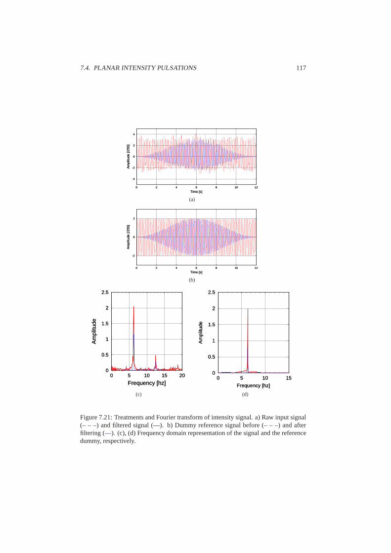
7.4. PLANAR INTENSITY PULSATIONS 117
-4
-2
0
2
4
0 2 4 6 8 10 12
Am
plitu
de [/
255]
Time [s]
-4
-2
0
2
4
0 2 4 6 8 10 12
Am
plitu
de [/
255]
Time [s]
(a)
-2
0
2
0 2 4 6 8 10 12
Am
plitu
de [/
255]
Time [s]
-2
0
2
0 2 4 6 8 10 12
Am
plitu
de [/
255]
Time [s]
(b)
0
0.5
1
1.5
2
2.5
0 5 10 15 20
Am
plitu
de
Frequency [hz]
0
0.5
1
1.5
2
2.5
0 5 10 15 20
Am
plitu
de
Frequency [hz]
(c)
0
0.5
1
1.5
2
2.5
0 5 10 15
Am
plitu
de
Frequency [hz]
0
0.5
1
1.5
2
2.5
0 5 10 15
Am
plitu
de
Frequency [hz]
(d)
Figure 7.21: Treatments and Fourier transform of intensitysignal. a) Raw input signal(– – –) and filtered signal (—). b) Dummy reference signal before (– – –) and afterfiltering (—). (c), (d) Frequency domain representation of the signal and the referencedummy, respectively.

118 CHAPTER 7. EXPERIMENTAL OBSERVATION OF TD INSTABILITIES
0
2
4
6
8
10
12
0 5 10 15 20 25 30
freq
uenc
y [1
/s]
U2/Dth [1/s]
0
2
4
6
8
10
12
0 5 10 15 20 25 30
freq
uenc
y [1
/s]
U2/Dth [1/s]
Figure 7.22: Pulsation frequency scaling with the diffusion frequency. The data doesnot scale as expected from the linear stability theory when the parameterωI is assumedconstant.
Name Symbol Units
Pulsation frequency f s�1Thermal diffusivity Dth m2 s�1Bulk velocity U m s�1Specific heat Cp J kg�1 K�1 = m2 s�2 K�1Flame Temperature Ta K
Table 7.2: List of parameters considered for the dimensional analysis of the pulsationfrequency scaling.
are not related by a simple power law, except at the larger values of the heat release pa-rameter. Other quantities involved in the phenomenon and not included in the analysiscan be responsible for the scatter observed. For instance, when only data points havingsimilar values for bothφ, Leo andLef , the linear relationship becomes clearer, as canbe seen from the third dataset plotted in figure 7.23. Accordingly, assuming constantLewis numbers and mixture strength, the influence of the bulkvelocity vanishes andthe pulsation frequency can be expressed as:
f � CpTf
Dth(7.3)
These results offer only limited insight on the phenomenon,hinting that someother relevant parameter was overlooked in the dimensionalanalysis. The groupf �Dth2U2 appears the proper dimensionless form for the frequency because its valuevaries around unity butCp � Tf 2U2 is suspicious because of its extremely large mag-nitude. As an alternative dimensionless expression of the chemical heat release, theDamkohler number given in equation 3.20 is promising as it contains the Arrheniusfactor which can possibly account for the non-power law relation of figure 7.23.

7.4. PLANAR INTENSITY PULSATIONS 119
10-2
10-1
100
101
1010 1011
f*D
th/U
2
CpTa/U2
10-2
10-1
100
101
1010 1011
f*D
th/U
2
CpTa/U2
10-2
10-1
100
101
1010 1011
f*D
th/U
2
CpTa/U2
10-2
10-1
100
101
1010 1011
f*D
th/U
2
CpTa/U2
Figure 7.23: Pulsation frequency scaling obtained from dimensional analysis, with boththe dataset gathered at constant inert composition (2) and constant velocity (b) shown.The agreement between the two datasets is best when the flame mixture strength issimilar (Q).
Scaling with Damkohler number
The experimental determination of the Damkohler number isnot trivial, as can be seenby the large number of parameters involved in its definition,reproduced in equation7.4. The main difficulty resides in finding suitable values for the activation energyE and the Arrhenius pre-exponential factorB. The activation energy is especiallytroublesome since it must be determined experimentally from measured reaction rateconstants. The data available in the literature for methaneis limited [164] and validonly for specific reaction temperature and value ofB. This pre-exponential factorBcan be estimated analytically but often differs significantly from experimental values.Fortunately, it exhibits only a limited dependence on temperature and is not a importantterm in the Dankohler number expression.Da � λ
ρacpU2�R0Ta
EE3
νxcpW
qR0WfPBXf,�� exp<�E2RTaA (7.4)
In equation 7.4, the terms expected to have a dominating influence in the change ofthe Damkohler number between the flames studied here areDth2U2, <R0Ta2EA3 andespeciallyexp<�E2R0TaA. Accordingly and because of the restrictions on the avail-able data, all of the other parameters andE are assumed constant. The Damkohlernumber used in this section is a relative one, calculated with respect to a flame arbi-trarily selected in the available dataset and assumed to have Da � 1. The measureddimensionless frequencyf �Dth2U2 as a function of this Damkohler number is shownin figure 7.24(a). In this figure, the correlation is much closer to a power law than in theprevious cases. However it appears that, as in section 7.4.2, the two datasets gatheredusing constant mixture properties and constant velocity have approximately the samepower law exponent but different pre-factors.
The first clues explaining this difference were found after systematic visual in-spection of the videos. The spread observed in the data of figure 7.24(a) was foundto be correlated to the difference in amplitude between the various pulsating flames

120 CHAPTER 7. EXPERIMENTAL OBSERVATION OF TD INSTABILITIES
measured. As a initial approach, the video were simply categorized as almost stable(weakly pulsating), pulsating and almost extinct (high amplitude pulsations). The re-sults plotted in figure 7.24(a) show a clear correlation for all three types of flames,with a slope in the log-log graph roughly equal to0.5. Most of the data available wascomprised of steady-state pulsation of medium amplitude because flames with similaraspect were desired to avoid saturation and under exposition in the videos. Using onlythis dataset of flames with similar pulsation amplitudes, the following correlation wasfound (plotted with the solid line in figure 7.24(a)):
fDth
U2� 0.909 �Da0.45 (7.5)
The dimensionless frequency therefore scales roughly withthe square root of theDamkohler number, at constant amplitude. The coefficient of determinationR2 of thiscorrelation is excellent at 0.97. For simplicity, the square root ofDa will be used as anapproximation when further refining this correlation. Unfortunately, it was impossibleto gather enough data points to verify if this relation stillhold true for very high orvery low pulsation amplitudes. The high amplitude flames aredifficult to capture sincethey often quickly lead to extinction. On the other hand, lowamplitude flames are hardto identify without complex video analysis. They are usually discarded as stable fromvisual inspection during the experiment, except during systematic experiments on theinstability onset. The few data points available with flame close to the marginal stateseem to indicate that a similar relationship can be found in those conditions.
The amplitude was measured quantitatively following the technique described atthe beginning of section 7.4.2 with the resulting data plotted in figure 7.24(b). Thetrend observed with the naked eye in the videos is visible in this figure, with the flamesclose to the marginally stable state having an amplitude lower than the average. Theflame identified as close to extinction have an amplitude significantly greater that theflames used to define the correlation of equation 7.5. The highest amplitudes mea-sured represent a variation in the measured light emission equal to over125% the av-erage value. In figure 7.24(c), the variation of the amplitude is shown as a function ofthe constant in equation 7.5, using an approximate value of0.5 for the power of theDamkohler number.
The limit-cycle oscillations observed are believed to be the result of supercriticalHopf bifurcation, like in the premixed configuration [165].This belief is confirmedby the substantial reactant leakage measured and reported in figure 7.20 and 7.8, indi-cating some degree of premixing associated with the instabilities. If it is the case, theStuart-Landau weakly non-linear stability theory [166] applies close to the bifurcationand predicts that the square of the oscillation amplitude should scale with the bifur-cation parameter. Using the correlation defined in equation7.5, yields the followingrelationship:
fDth
U2
pDa
� C0 � aǫ2 (7.6)
Whereǫ is the pulsation amplitude. This theoretical prediction isplotted as thesolid line in figure 7.24(c). The constantsC0 is the dimensionless frequency divided
byp
Da when the amplitude is zero, corresponding to the marginallystable state.This value could be estimated directly from the available experimental data at very lowamplitude. The value of the parametera was then determined through the correlationfound with the whole experimental dataset. By adjusting thevalue ofC0 slightly to
7.4. PLANAR INTENSITY PULSATIONS 121
maximize the correlation coefficient, it was possible to achieve a correlation in qualita-tive agreement with the theoretical prediction, with the amplitude raised to the power1.67. However, theR2 for the correlation remained low at about0.6. It should be em-phasized here that the confidence in the amplitude data gathered in this experiment islimited because mainly of the spatial integration imposed by the acquisition techniqueused (see section 7.4.2).
The ratio of the fundamental to the first harmonic of measuredintensity signal wasalso calculated. According to weakly non-linear stabilitytheory, the amplitude of thefirst harmonic should be proportional to the square of the amplitude of the fundamen-tal. Attempts were made to verify this relationship, but theavailable amplitude dataproved too unreliable to yield conclusive results. The spatial integration of the flamelight emission inherent to the acquisition method used thatcauses an amplitude modu-lation when two regions of the burner pulsate at slightly different frequencies or out ofphase. An example of such a modulated signal is given in figure7.18(c). Refinementsin the experiment should be implemented to investigate moredeeply the role of thepulsation amplitude in the frequency scaling. Such refinements should include tech-niques allowing spatially resolved measurements of the intensity variation with a widedynamic range. Recent development in sensitive temperature measurements based onoptical techniques offering the required bandwidth is a promising prospective solutiontowards this goal.

122 CHAPTER 7. EXPERIMENTAL OBSERVATION OF TD INSTABILITIES
10-2
10-1
100
101
10-4 10-3 10-2 10-1 100 101 102
f*D
th/U
2
Da
10-2
10-1
100
101
10-4 10-3 10-2 10-1 100 101 102
f*D
th/U
2
Da
10-2
10-1
100
101
10-4 10-3 10-2 10-1 100 101 102
f*D
th/U
2
Da
10-2
10-1
100
101
10-4 10-3 10-2 10-1 100 101 102
f*D
th/U
2
Da
10-2
10-1
100
101
10-4 10-3 10-2 10-1 100 101 102
f*D
th/U
2
Da
10-2
10-1
100
101
10-4 10-3 10-2 10-1 100 101 102
f*D
th/U
2
Da
10-2
10-1
100
101
10-4 10-3 10-2 10-1 100 101 102
f*D
th/U
2
Da
10-2
10-1
100
101
10-4 10-3 10-2 10-1 100 101 102
f*D
th/U
2
Da
(a)
10-4 10-3 10-2 10-1 100 101 102
10-210-1100101 0
0.25
0.5
0.75
1
1.25
1.5
Pul
satio
n am
plitu
de [r
elat
ive]
Daf*Dth/U210-4 10-3 10-2 10-1 100 101 102
10-210-1100101 0
0.25
0.5
0.75
1
1.25
1.5
Pul
satio
n am
plitu
de [r
elat
ive]
Daf*Dth/U210-4 10-3 10-2 10-1 100 101 102
10-210-1100101 0
0.25
0.5
0.75
1
1.25
1.5
Pul
satio
n am
plitu
de [r
elat
ive]
Daf*Dth/U210-4 10-3 10-2 10-1 100 101 102
10-210-1100101 0
0.25
0.5
0.75
1
1.25
1.5
Pul
satio
n am
plitu
de [r
elat
ive]
Daf*Dth/U210-4 10-3 10-2 10-1 100 101 102
10-210-1100101 0
0.25
0.5
0.75
1
1.25
1.5
Pul
satio
n am
plitu
de [r
elat
ive]
Daf*Dth/U210-4 10-3 10-2 10-1 100 101 102
10-210-1100101 0
0.25
0.5
0.75
1
1.25
1.5
Pul
satio
n am
plitu
de [r
elat
ive]
Daf*Dth/U2
(b)
10-2
10-1
100
10-1 100 101
Am
plitu
de [r
elat
ive]
f*Dth/(U2*Da0.5) - C0
10-2
10-1
100
10-1 100 101
Am
plitu
de [r
elat
ive]
f*Dth/(U2*Da0.5) - C0
10-2
10-1
100
10-1 100 101
Am
plitu
de [r
elat
ive]
f*Dth/(U2*Da0.5) - C0
(c)
Figure 7.24: a) Scaling of the pulsation frequency with the Damkohler number, with thedifferent flame types observed: almost stable (b, Y), medium amplitude pulsations (2,i) and almost extinct (Q, M). The open and filled symbols are from datasets gatheredat constant inert inert composition and constant velocity,respectively. b) Measuredpulsation amplitude for the data in (a). c) Scaling taking into account the pulsationamplitude, withC0 � 0.05 used.

Chapter 8
Conclusions and outlook
The burner presented in this thesis has evolved from the firstexperimental realizationof a one-dimensional chambered diffusion flame [55, 96]. Thenovel symmetric designof the reactant supply to the combustion chamber allows the investigation of the effectof bulk flow magnitude and direction on a diffusion flame in theabsence of signifi-cant strain. The improvements introduced in the present version of the burner allowa reduction of the parasitic flame curvature and residual strain observed in the initialimplementation of the design. One important innovation is the use of a quartz cylinderplaced inside the burning chamber to separate the more homogeneous central portionfrom the edges where velocity, species and temperature gradients exist. The result isthe creation of a very flat flame inside the cylinder, where allthe measurements arecarried out.
The practical difficulty with this design which is due to the unknown proportion offuel and/or oxidant lost into the exhausts has been overcomeby the systematic use ofmass spectroscopy in the combustion chamber. The key to the successful use of themass spectrometer in this situation with large concentration variations is an innovativecalibration procedure which yields continuous concentration profiles of the four or fivespecies present in the burner and permits the determinationof the effective mixturestrength of the flame. The relative error in the measurement of this important flame pa-rameter is estimated to be on the order of 5%, a precision thatcould not be approachedwithout the novel calibration developed in this study.
In addition to the mass spectrometric measurements, a detailed characterization ofthe burner and flame produced has been achieved by using advanced experimental tech-niques. The fluid flow in the burner has been measured using LDAand has alloweda precise quantification of the residual strain experiencedby the flame front, whichwas determined to be below0.15 s�1. The flame temperature was determined usingthermocouple probes, constructed to avoid conduction losses and catalytic effects. Theradiation corrected maximum measured temperature agree within 50 K with the flametemperature as determined from numerical adiabatic calculations. The measurementsregarding the homogeneity of the species and temperature distribution in the centralpart of the burner have revealed deviations below125 K in the flame temperature and10 % in the counter-diffusing species volume fraction at the boundary. The good agree-ment between the present experiments and the simple theory for the flame position, thetemperature and the species concentration profiles demonstrates that our new symmet-ric burner is a good approximation of a chambered one-dimensional diffusion flame,with one species transported against the bulk flow by diffusion only.
123

124 CHAPTER 8. CONCLUSIONS AND OUTLOOK
The central contribution of this study has been the quantitative documentation andanalysis of thermal-diffusive instabilities close to extinction. The use of a two inertmixture (helium and CO2) as dilution for the reactants has allowed a wide range ofLewis numbers to be investigated. The type of instabilitiesobserved close to extinctionhas been mapped in the Lewis number parameter space for both hydrogen and methaneflames burning with oxygen. In hydrogen flames, a cellular structure was observed forthe low Lewis numbers associated with a dilution gas comprised mostly of CO2. Thecharacteristic size of the cellular pattern was observed togrow as the Lewis numberincreased when CO2 was replaced by helium in the inert. It ranged from about7 mmfor flames diluted in pure CO2 to 15 when mostly helium was used. The cell size scaledrather close to linearly with the diffusion lengthlD, in good agreement with theoreticalpredictions.
The transition from cellular to intensity pulsations as thedominant mode of in-stability close to extinction occurred for hydrogen flames when80% of the dilutionmixture was helium. The weak light emission of these H2 pulsating flames preventedtheir detailed investigation and methane flames where used to study the phenomenonfor the first time in an essentially unstrained setting. Pulsation frequencies in the rangeof 0.6 to 11 Hz were observed in these flames using the same two inerts for dilution.A correlation was found for the scaling of the pulsation frequency as a function of theflame parameters: the pulsation frequency multiplied by thethermal diffusion time wasfound to scale approximately with the square root of the Damkohler number.
For the first time, theoreticians now have experimental datain unstrained diffusionflames available to validate their models. Direct comparison between observations andthe theoretical predictions is however not trivial beyond what has been done in thisthesis because of the limited parameter range which it is possible to explore experi-mentally. In the experiment, one also observes saturated modes while the theory ispresently limited to infinitesimal perturbations. Nevertheless, with this in mind futuretheoretical and numerical investigations can be designed specifically to allow quantita-tive comparisons.
On the definition of the mixture strength φ
The experimental results gathered in this thesis have revealed the limitations of thecurrently used definition of the mixture strengthφ. The virtual origin technique im-plemented in section 6.5 to compensate for the velocity or density induced variationof the boundary conditions while keeping a constantφ illustrates the arbitrary natureof this definition. Theφ stays constant because the concentration of the oxidant at theboundary has not changed, but the distance between the flame and the boundary haschanged. Surely from theflame point of viewthe situation must be different.
Let’s consider an example in the configuration most frequently used in this thesis,with the oxidant counter-diffusing against the bulk flow. For a given flame a certainamount of oxidant is present at the boundary, of which only a fraction will manage toreach the reaction zone. Now, to compensate for the increasein the oxidant volumefraction at the boundary following a decrease in bulk velocity a new virtual originis taken upstream of the initial boundary position. At this new location, the amountof oxidant is the same as in the previous case; What has changed is the value of theexponential in the concentration profile of equation 3.15. The definition of the mixturestrength should therefore include not only how much of the counter-diffusing reactantis supplied but also how it is supplied. As new quantity, for instance the maximum

125
slope of the mass fraction of the counter-diffusing speciesat the flame, might be auseful and physically more meaningful measure of the ratio of the supplied fuel to theavailable oxidant, weighted by the stoichiometric ratio.
Future work
The numerous improvements implemented and the detailed characterization carried outin the new version of the burner have yielded a clear picture of the configuration pre-sented in this thesis. Refinements are still possible and have been identified to bring thisexperimental realization still closer to the idealized one-dimensional construct. One ofthe main issues is the management of heat losses, particularly in the chimney sincethey are believed to be at the origin of the most detrimental wall effects observed inthe burner, that is the variation in the counter-diffusing species boundary condition.Resulting in flame front curvature and residual stretch. Oneoption to improve this sit-uation would be to use a fluid or paste with a high thermal conductivity in the chimneyto improve the heat transfer between the injection and extraction tubes. The use of elec-trical heating in this region of the burner is also a possiblesolution, but in both casestemperature inhomogeneities will probably remain, albeitwith a lower magnitude thanis currently observed. A more definitive solution to this issue would be to place if notthe whole burner, at least the chimney in an oven heated to thetemperature of the ex-haust gas. This would however require a considerable increase in the complexity of theexperiment to maintain optical and physical probing accessto the combustion chamber.
The use of more advanced experimental techniques could alsohelp to resolve re-maining issues. In particular, laser based temperature andspecies measurements couldprovide a drastic improvement in dynamic range of the measurement of planar inten-sity pulsations. This is of course provided that sufficient bandwidth could be achievedto temporally resolve the phenomenon. The technique would also allow the spatialresolution of the pulsation, avoiding the problems encountered with spatially integrat-ing techniques such as the one used in this thesis when parts of the flame pulsate outof phase with each other. The results gathered in this way would more importantlyprovide a reliable measurement of the pulsation amplitude,allowing more in-depthanalysis on the nature of the instabilities present and its scaling. Using such techniquesmight also permit to further investigate very weakly luminous phenomena that couldonly be observed with the naked eye in this study, such as pulsations or rotating spiralsin hydrogen flames.
The effect of heat loss to the injection array on the thermal diffusive instability isalso difficult to evaluate in this experiment, but is likely to have a significant effect. At-tempts to quantify this process, either experimentally or analytically, would be usefulsince heat loss is known to play a role in thermal-diffusive instabilities. For instance,Cheatham and Matalon [167] have demonstrated that intensity oscillation can be trig-gered both by high Lewis number without heat loss and by high heat loss, even forrelatively small Lewis numbers.
The symmetric burner design introduced here is in particular aimed at the first in-vestigation of a purely diffusive unstrained flame in the zero bulk flow limit. Exper-iments have been conducted to generate such a flame but have not met with success.These attempts involved starting with a stable flame and a small bulk flow, then openthe extraction plenum of the advected species to remove the bulk flow by allowing theproducts to escape symmetrically. However, as this happened, the flame always col-lapsed on one of the injection arrays, either partially or totally. Once this condition

126 CHAPTER 8. CONCLUSIONS AND OUTLOOK
developed, it was very difficult or impossible to stabilize the flame front in the middleof the burner, even after one of the exhaust plenums was againclosed. More experi-ments need to be made before the realization of such a purely diffusive flame withoutbulk flow can be ruled out. Perhaps some kind of active controlis required in the pres-sure drop between the exhaust plenums. It might also be useful to try placing differentdevices inside the burning chamber to keep the flow one dimensional and prevent theformation of convection cells believed to be at the origin ofthe partial flame front col-lapse. A honeycomb structure might be useful for this task. Alternatively, the burnercould be lit with both exhausts already open. This last option was not tried during theintense measurement sessions leading to this thesis for fear that the stronger explo-sions resulting from ignition in a quiescent chamber with a larger volume of explosivemixture would damage the equipment.
Research opportunities
The novel burner configuration presented in this thesis has only been used so far toinvestigate thermal-diffusive instabilities in the absence of strain. However, the possi-bility to generate such unstrained diffusion flames also offers new and unique opportu-nities in other fields of research. For example, to generate planar intensity pulsations,rich methane flames were produced and the formation of a highly luminous soot layeron the fuel side of the flame was noticed. A snapshot is shown infigure 8.1 where abright yellow band is visible below the flame. The conditionsunder which this chanceobservation was made could be optimized specifically to improve the one-dimensionalcharacter of the soot layer. The burner design used in this thesis could therefore be usedas a new tool to investigate the effect of strain and in particular the absence of strain onthe formation of soot in hydrocarbon flames. Research on the subject has so far beenlimited to flame configurations where strain is always present [48, 168].�� � �Figure 8.1: Chance observation of a soot layer forming on thefuel side of a richmethane flame.
Diffusion flames of methane and oxygen can also used for the production of car-bon nanotubes [169]. This discovery was made while investigating the effect of thethe strain rate on the microstructure of the soot formed in anopposed jet flame. Thetechnique is novel because it provides a means to continuously produce this promisingmaterial, in contrast to the batch processes typically usedtoday. The strain has beenobserved to have an effect of the structure of the carbon clusters formed. An unstrainedflame would therefore be a useful research tool to investigate the parameters relevantto carbon nanotubes formation in diffusion flames without aerodynamic perturbations.

Appendix A
Mass spectrometer systemanalysis
The initial trials of the instrumentin situ revealed that its complex and sometimes un-predictable response to the numerous complicating aspectsof this experiment (wideconcentration range, presence of reactive species, etc.) would require a detailed anal-ysis of the system to understand its intricacies. In this section, the pressures and flowrates through the different components of the mass spectrometer are determined. Thiswill allow in the next two section the identification of the sources of non-linearity andthe implementation of an appropriate calibration procedure.
This mass spectrometer is designed to be able to sample gas mixtures directly atatmospheric pressure. Before analysis, the pressure of thesample must the be lowereddrastically to bring it to a state where the molecules are farenough apart to stop inter-acting with each other. Such a rarefied gas is said to be in molecular flow, its motion nolonger governed by pressure differentials but only by the random kinetic velocity of theatoms and molecules it contains. This velocity of the molecules will play a critical rolein the dynamics of the sample transmission between the different parts of the system.The velocity distribution of the molecules in a gas follows the Maxwell-Boltzmann dis-tribution and quantities such as the mean speed of the moleculesva will characterizethe gas ability to move in free molecular flow.
va �r8κT
πm�r8RT
πM(A.1)
Hereκ � R2NA � 1.38e�23 is the Boltzmann constant,R � 8.3144 the perfect gasconstant,NA � 6.022e23 Avogadro’s number,T the temperature,m the mass of theparticle andM the molecular weight. From this equation, it is obvious thatthe meanspeed and hence many features of the system, is gas specific. For the numerical appli-cations presented in this section, the mean molecular speedof CO2 at 300 K, whichis 379.9 m/s, will be used since this species usually makes up most of the mixturesanalyzed.
A.1 Working pressures
To verify that the molecular flow assumption is reasonable for the different parts ofthe system, it is necessary to compare the mean free path (L) of the molecules with a
127

128 APPENDIX A. MASS SPECTROMETER SYSTEM ANALYSIS
characteristic length scale (a). The resulting ratio is called the Knudsen number (Kn)and forKn 1 1 a gas can be considered in free molecular flow. ForKn 0 0.01 the flowis considered viscous and the usual equations of fluid mechanics can be used. Betweenthose two extreme values correction factors can be applied to either the viscous ormolecular equations to properly capture the transitory nature of the flow.
Kn � L
a(A.2)
L � RTp2πd2NAP
(A.3)
In this system the temperature is regulated to avoid condensation so the mean freepath will be mostly a function of the pressure maintained in the different components ofthe instrument. A schematic representation of the samplingand analysis system of theMKS Cirrus is presented in figure A.1. In vacuum systems, the ability of a channel toallow the flow of gas is usually represented by the conductanceC [170]. This quantitycorresponds to the rate of flow (throughput)Q per unit of pressure difference betweenthe two ends of the channel. The units of the conductance ism32s so the throughputQ is not a volumetric flow rate, it is a quantity that illustrates the mass flow, a pressuremultiplied by a volume.
C � Q
P2 � P1(A.4)
The components used to create three successive pressure drops in the sample as it istransported towards the mass filter are presented with theirconductances in table A.1.The resulting pressure variation experienced by the sampleand the associated changein the mean free path are summarized in table A.2. The values of the pressures at pointB was communicated by the manufacturer and a total pressure gauge gives the pressurein the vacuum chamber D. The rest of the values had to de determined analytically.
DiaphragmPump
TurbumolecularPump
DetectorMass FilterCapillary Input Bypass Ion Source
1
2
34
5
67
A
B
CD
Figure A.1: Schematic representation of the vacuum system of the mass spectrometer.1. The capillary input, 2. Bypass line, 3. Orifice, 4. Ionization chamber, 5. Exhaustline. The conductances and pressures of the various components are presented in tablesA.1 and A.2.

A.1. WORKING PRESSURES 129
Component Label in figure A.1 Conductance[m3/s]
Capillary line 1 3.41e-9Orifice plate 3 6.71e-8Ion source 4 2.23e-4
Table A.1: Conductance values (for CO2) for the different components of the vacuumsystem
RegionLabel
fig. A.1Pressure
MeanFree Path
Kn
Nominal Measured[mbar] [mbar] [m] [ ]
Sampling A 970 970 6.02e-8 6.02e-4Bypass B 5 5 11.66e-6 0.78Ion. Chamber C 1.51e-3 1.50e-3 38.33e-3 38.33Vacuum chamber D 1e-5 4e-6 9.60 192
Table A.2: Values of pressures and mean free paths throughout the vacuum system.
As can be seen in table A.2 the flow at the sampling end of the capillary is obvi-ously viscous. The expression given in equation A.6 for the volumetric flow rate andthe conductance of the capillary can therefore be estimatedusing the Hagen-Poiseuilleequation A.6[171]. This requires the flow to be laminar as will be verified once theflow rate is known. HereV is the volumetric flow rate,r � 0.05mm is the radius of thetube,l its length andµ the dynamic viscosity. Here the termPa, the average pressure,is added to yield a mass flow rateQ consistent with the rest of our development. Thisrelation is only an approximation since thermal and compressibility effects can signifi-cantly change the result [172, 173, 174], but will be sufficient for a first approach.
V � πr4
8µl∆P (A.5)
CCapil � πr4
8µlPa (A.6)
Using this conductance, adding the conductance from the bypass line 2 in fig. A.1,and using the specifications of the bypass pump, it is possible to determine the pressurein the bypass chamber, labeled B in figure A.1. This pressure is important becauseit controls the flow rate inserted in the ionization chamber and hence its operatingpressure. Using various models to evaluate the conductanceof the bypass line in thetransition regime (Kn Æ 0.05)[175], the pressure in the bypass chamber was estimatedto be between1 and2 mbar. These values are considerably lower than the nominalvalue of5 mbar supplied my MKS. For the remainder of the calculations,the bypasschamber pressure was assumed to be5 mbar, considering it to be a safe upper boundfor this parameter. However, the implications of considering a lower value for thispressure will be briefly discussed.

130 APPENDIX A. MASS SPECTROMETER SYSTEM ANALYSIS
The sample present in the bypass chamber is supplied to the ionization chamberthrough a disk, labeled 3 in figure A.1, with an array of 4 holesof 15 µm diameter tofurther reduce the pressure. The ion source enclosure, label 4 in fig. A.1, is pumpedthrough 3 holes of 1 mm diameter exiting in the main vacuum chamber pumped bythe turbomolecular pump. The pressure in this chamber is available through a totalpressure penning gauge. To determine the pressure inside the ionization chamber, acritical parameter to determine the nature of the ionization process, it is then necessaryto calculate the conductances of the orifice disk and the ion source enclosure.
The conductance of a circular orifice, in the molecular flow regime, is given byequation A.7, whereA is the area of the orifice andva is the mean molecular speed.The total conductance of the orifice plate (COr) and ion source enclosure is then simplyfound by summing the conductances of the individual holes allowing gas exchange ineach component. The resulting numerical values for the conductances for CO2 at 300
K are given in table A.1.
COrifice � 1
4vaA (A.7)
From the values of the mean free path and Knudsen numbers presented in tableA.1, one might argue that the flow in the orifice plate holes is not molecular but actuallytransitory. The value ofKn � 0.78 (based on the orifice diameter) for CO2 is in facta conservative estimate because all the other species having a smaller diameter, theirmean free path is longer. For example in the same situation the Knudsen number forhydrogen is1.41 and1.05 for both oxygen and argon. Moreover, a slight increase intemperature also has the effect of increasing the mean free path and Knudsen number.For instance if heating is used to avoid condensation, as it often is, the temperature inthe bypass region becomes80XC and the Knudsen number for CO2 is 0.91. The valuesfor the hard sphere collision diameters of the various molecules and atoms were foundin the literature[163].
Nevertheless, if we consider the viscous nature of the flow inthe orifice, the con-ductance of this element can be determined using equation A.8[176] assuming a negli-gible plate thickness and isentropic gas expansion. In thisequationγ is the isentropicexpansion factor, which is equal to1.30 for CO2 at room temperature[171]. The result-ing viscous conductance of the 4 orifice of the plate is181.98e � 9 m3/s, so about 2.7times more than in the molecular regime.
COr,V iscous � suutπγ
8? 2
γ � 1D γ�1
γ�1vaA (A.8)
The pressure inside the ionization chamber is found by solving successively theequation of the conductance A.4 between points B and C then between points C and D,assuming a constant mass flow rate. Assuming that the flow is molecular in the orificeplate 3, the pressure in the ionization chamber is1.50e � 3 mbar. In the unlikely eventthat the viscous regime dominates in the holes of this component, the upper bound forthe pressure inside the ion source enclosure is4.07e�3 mbar. These values are obtainedassuming a5 mbar bypass chamber pressure. If the pressure is1 mbar, the flow rate tothe ionization chamber is reduced and its pressure falls to3.00e � 4 mbar
A.2. SAMPLING RATE AND IONIZATION EFFICIENCY 131
A.2 Sampling rate and ionization efficiency
The flow rate sucked from the flame can be found using the capillary conductancedetermined in the previous section and equation A.4. The resulting molar flow rateis 131.92E � 9 mol/s. This corresponds to1.77e � 4 SLPM, a negligible proportion(0 1250�000) of the approximatively10 SLPM bulk flow in the burner.
The resulting velocity is0.432 m/s at the entrance and83.83 m/s at the exit. Thisimplies a maximum Reynolds number based on the tube diameterof ReD � V d2ν �4.91, confirming that the flow is laminar since the very narrow cross-section of thetube.
The actual flow rate entering the ion source through the orifice plate (label 3 infigure A.1) is determined by considering the conductances ofthe orifice plate and theion source enclosure connected in series. The total impedanceZTot � 12CTot of thispart of the circuit can be found by adding the impedance of theorifice and ion source.
1
CT ot� 1
COr� 1
CIS(A.9)
Assuming molecular flow in the orifice, the resulting molecular flow rate is13.45e�9 mol/s, or8.10e15 molecules per seconds (the bypass ratio is then about 10), implyinga9.81 bypass ratio. Considering that the total ionic current detected by the instrumentsupplied with pure CO2 is approximately3.85e � 9 A, or 24.02e9 charges per sec-ond, this corresponds to a combined ionization and detection efficiency of2.96e � 4%.In other words, for CO2 one out of every337�000 molecules inserted in the vacuumchamber is detected. These values rely on the assumption that the pressure in the by-pass chamber is5 mbar. If instead we use the1 mbar estimation from the hardwarespecifications, we find a flow rate into the ionization chamberof 2.26e � 9 mol/s. Inthis case, the bypass ratio is58.4 and the ionization efficiency1.77e � 3% or one outof every56�600 molecules ionized and detected.
For these flow rate calculations, the conductances of the bypass line and the tur-bomolecular pump inlet (labels 2 ant 5 in figure A.1) where evaluated conservativelyusing standard formulas[170, 175] and the available geometrical information. They arefound to offer significantly less resistance to the gas flow than the capillary and theorifice plate and hence play only a minor role in the final values of the pressures andflow rates.


Appendix B
Possible reactant and inertcombinations
The choice of the reactants (hydrogen and methane) and inerts (helium and CO2) usedin the experiments presented in this thesis is the result of an thorough selection process.Two inerts are required to generate the range of transport properties sought to coveras much as possible of the Lewis number parameter space. Other gases combinationwere considered to generate the largest possible range of Lewis numbers. The useof noble gases for the inerts seemed very attractive at first because of their inherentstability and reliable detection by mass spectrometry. However, the use of two noblegas as inerts plus the two reactants and the two products (H2O and CO2) resulting fromcarbon-based fuel combustion would require a 6 gas mass spectrometer calibration.The complexity of this task forces the use of CO2 as one of the inerts for all carbon-based fuels. For hydrogen, CO2 must also be used to ensure that the flame emits enoughlight to be visible. Other species with similar properties could be used, but CO2 wasused in hydrogen flames as well to avoid complications. Nitrogen for instance, which isless stable than CO2 at high temperature, resulting in the formation of nitrogenoxidesthat should be accounted for in the calibration procedure.
To produce the high Lewis numbers necessary to observe the planar intensity pulsa-tions described in section 7.4 required the use of either heavy fuels of light inerts. Bothof these choices had drawbacks that had to be weighted in order to find the optimal gascombination. The light inert chosen was naturally helium because of its extremely lowmolecular mass, very good high temperature stability and affordable prices. The Lewisnumbers covered using these inerts and some other on three different fuels burning inhydrogen is given in figure B.1.
The use of heavier carbon-based fuels would necessitate extensive re-calibration ofthe mass spectrometry system of the implementation of another technique to measurethe effective mixture composition in the burning chamber. These heavier fuels are alsoassociated with increased source and mass filter fouling in quadrupole mass spectrom-eters. The formation of soot in the chamber would also be an issue, preventing opticalaccess to the chamber and necessitating frequent cleanup.
133

134 APPENDIX B. POSSIBLE REACTANT AND INERT COMBINATIONS
0
0.25
0.5
0.75
1
0.5 1 1.5 2 2.5
Lef [
]
Lex [ ]
0
0.25
0.5
0.75
1
0.5 1 1.5 2 2.5
Lef [
]
Lex [ ]
0
0.25
0.5
0.75
1
0.5 1 1.5 2 2.5
Lef [
]
Lex [ ]
0
0.25
0.5
0.75
1
0.5 1 1.5 2 2.5
Lef [
]
Lex [ ]
(a) Hydrogen
0
0.5
1
1.5
2
2.5
0.5 1 1.5 2 2.5
Lef [
]
Lex [ ]
0
0.5
1
1.5
2
2.5
0.5 1 1.5 2 2.5
Lef [
]
Lex [ ]
0
0.5
1
1.5
2
2.5
0.5 1 1.5 2 2.5
Lef [
]
Lex [ ]
0
0.5
1
1.5
2
2.5
0.5 1 1.5 2 2.5
Lef [
]
Lex [ ]
(b) Methane
0
0.5
1
1.5
2
2.5
0.5 1 1.5 2 2.5
Lef [
]
Lex [ ]
0
0.5
1
1.5
2
2.5
0.5 1 1.5 2 2.5
Lef [
]
Lex [ ]
0
0.5
1
1.5
2
2.5
0.5 1 1.5 2 2.5
Lef [
]
Lex [ ]
0
0.5
1
1.5
2
2.5
0.5 1 1.5 2 2.5
Lef [
]
Lex [ ]
(c) Butane
Figure B.1: Lewis number parameter spaces covered using hydrogen, methane andbutane as the fuel. The inert mixtures considered are He and CO2 (2), He and Ar (b),He and Xe (Q) and CO2 and Xe (S).

Appendix C
Nomenclature
Notation
Latin alphabetB [m3/mol*s] Specific heat at constant pressureCp [J/kg*K] Specific heat at constant pressureDa [ ] Damkohler numberDi [m2/s] Diffusivity of speciesiDth � λ2<ρCpA [m2/s] Thermal diffusivityE [J/mol] Activation energyf [1/s] Pulsation frequencyK [1/s] Total stretch rateKc [1/s] Contribution of flame curvature to stretch rateKs [1/s] Strain rateLef � κ2Df [ ] Lewis number of fuelLeo � κ2Do [ ] Lewis number of oxidantLe [ ] Unique Lewis number or Lewis number of the most con-
sumed reactantP [Pa] Pressureq [J/kg] Heat released per unit mass of fuelQ [J/mol] Total heat releasedR [J/kg*mol] Ideal gas constantTa [K] Adiabatic flame temperatureU [m/s] Bulk flow velocityW [kg/mol] Mean molecular weightWi [kg/mol] Molecular weight of specieiXf [ ] Fuel mass fractionXo [ ] Oxidizer mass fractionx [m] Coordinate along burner length
Greek alphabet
ǫ [variable] Pulsation amplitude
135

136 APPENDIX C. NOMENCLATURE
λ [W/m*K] Thermal conductivityνi [ ] Stoichiometric coefficient of speciesiφ [ ] Equivalence ratio (mixture strength)ρ [kg/m3] Densityσ� [ ] Real part critical growth rate in the marginal stateω [mol/s] Chemical reaction rateωI [ ] Imaginary part of critical growth rate in the marginal state
ShorthandCCA : Constant current anemometryEI : Electron impact ionizationEPFL : Swiss federal institute of technology, LausanneFWHM : Full width half maximumID : Inner diameterLDA : Laser Doppler anemometryLIF : Laser induced fluorescenceLMF : Laboratory of fluid mechanicsMBMS : Molecular beam mass spectrometryOD : Outer diameterPPA : Partial pressure analyzerQMS : Quadrupole mass spectrometerRD : Reaction-diffusionRGA : Residual gas analyzerSEM : Secondary electron multiplierSLPM : Standard liters per minuteSLR : Single lens reflexTD : Thermal-diffusive

Bibliography
[1] S. R. James, R. W. Dennell, A. S. Gilbert, H. T. Lewis, J. A.J. Gowlett, T. F.Lynch, W. C. McGrew, C. R. Peters, G. G. Pope, A. B. Stahl, and S. R. James.Hominid use of fire in the lower and middle pleistocene: A review of the evi-dence.Current Anthropology, 30(1):1–26, 1989.
[2] Dick Stapert and Lykke Johansen. Making fire in the stone age: flint and pyrite.Geologie en Mijnbouw, 78:147–164, 1999.
[3] N. Kunzli, R. Kaiser, S. Medina, M. Studnicka, O. Chanel, P. Filliger, M. Herry,V Puybonnieux-Texier F. Horak Jr, P. Qunel, J. Schneider, R.Seethaler, J.-C.Vergnaud, and H. Sommer. Public-health impact of outdoor and traffic-relatedair pollution: a european assessment.The Lancet, 356:795–801, 2000.
[4] J. T. Houghton, G .J. Jenkins, and J. J. Ephraums, editors. Climate change: TheIPCC scientific assessment. Cambridge University Press, 1990.
[5] J. T. Houghton, Y. Ding, D. J. Griggs, M. Noguer, P. J. van der Linden, X. Dai,K. Maskell, and C. A. Johnson, editors.Climate Change 2001: The ScientificBasis. Cambridge University Press, 2001.
[6] N. P. Tait. Soot formation in cracked flames.Combustion and Flame, 117(1-2):435–437, 1999.
[7] D. Bradley, C. G. W. Sheppart, R. Woolley, D. A. Greenhalgh, and R. D. Lock-ett. The development and structure of flame instabilities and cellularity at lowmarkstein numbers in explosions.Combustion and Flame, 122(1-2):195–209,2000.
[8] A. M. Turing. The chemical basis of morphogenesis.Phil. Trans. of the RoyalSoc. of London B, 237(641):37–72, 1952.
[9] A. Cho. Lifes patterns: No need to spell it out?Science, 303:782–783, 2004.
[10] Philip K. Maini, Ruth E. Baker, and Cheng-Ming Chuong. The turing modelcomes of molecular age.Science, 2006.
[11] Stefanie Sick, Stefan Reinker, Jens Timmer, and ThomasSchlake. Wnt and dkkdetermine hair follicle spacing through a reaction-diffusion mechanism.Science,314:1447, 2006.
[12] Han-Sung Jung, Philippa H. Francis-West, Randall B. Widelitz, Ting-XinJiang, Sheree Ting-Berreth, Cheryll Tickle, Lewis Wolpert, and Cheng-Ming
137

138 BIBLIOGRAPHY
Chuong. Local inhibitory action of bmps and their relationships with activa-tors in feather formation: Implications for periodic patterning. DevelopmentalBiology, 196:11–23, 1998.
[13] Isaac Salazar-Ciudad and Jukka Jernvall. A gene network model accounting fordevelopment and evolution of mammalian teeth.Proc. Nat. Acad. Sci. USA,99(12):8116–8120, 2002.
[14] V. Castets, E. Dulos, J. Boissonade, and P. De Kepper. Experimental evidenceof a sustained standing turing-type nonequilibrium pattern. Physical ReviewLetters, 64(24):2953–2957, 1990.
[15] I. Lengyel and I. R. Epstein. A chemical approach to designing turing patternsin reaction-diffusion systems.Proc. Nutl. Acud. Sci. USA, 89:3977–3979, 1992.
[16] Julyan H. E. Cartwright. Labyrinthine turing pattern formation in the cerebralcortex.J. theor. Biol., 217:97–103, 2002.
[17] John E. Pearson. Complex patterns in a simple system.Science, 261(5118):189–192, 1993.
[18] C. B. Muratov and V. V. Osipov. Scenarios of domain pattern formation in areaction-diffusion system.Phys. Rev. E, 54(5):4860–4879, 1996.
[19] W. Y. Tam, W. Horsthemke, Z. Noszticzius, and H. L. Swinney. Sustained spi-ral waves in a continuously fed unstirred chemical reactor.J. Chem. Phys.,88(5):3395–3396, 1988.
[20] K. J. Lee and H. L. Swinney. Lamellar structures and self-replicating spots in areaction-diffusion system.Phys. Rev. E, 1995.
[21] P. S. Hagan. Spiral waves in reaction-diffusion equations.SIAM J. App. Math.,42(4):762–786, 1982.
[22] William N. Reynolds, Silvina Ponce-Dawson, and John E.Pearson. Self-replicating spots in reaction-diffusion systems.Phys. Rev. E, 56(1):185–198,1997.
[23] S. Arrhenius. Uber die reaktionsgeschwindigkeit bei der inversion vonrohrzucker durch sauren.Z. Phys. Chem, 4:226, 1889.
[24] C. W. Wardlaw. A commentary on turing’s diffusion-reaction theory of morpho-genesis.New Phytologist, 52(1):40–47, 1953.
[25] J.E. Pearson and W. Horsthemke. Turing instabilities with near equal diffusioncoefficients.J. Chem. Phys., 90(3):1588–1599, 1989.
[26] G. I. Sivashinsky. Instabilities, pattern formation and turbulence in flames.Ann.Rev. Fluid Mech., 15:179–199, 1983.
[27] J. Buckmaster. The structure and stability of laminar diffusion flames.Ann. Rev.Fluid Mech., 25:21–53, 1993.
[28] P. Clavin. Premixed combustion and gasdynamics.Ann. Rev. Fluid Mech.,26:321–352, 1994.

BIBLIOGRAPHY 139
[29] Moshe Matalon. Intrinsic flame instabilities in premixed and nonpremixed com-bustion.Annu. Rev. Fluid Mech., 39:169–191, 2007.
[30] E. Mallard and E. Le Chatelier. Combustion des melanges gazeux explisifs.Ann.Mines, 8(3):274–378, 1883.
[31] A. K. Oppenheim and R. I. Soloukhin. Experiments in gas dynamics of explo-sions.Ann. Rev. Fluid Mech., 5:31–58, 1973.
[32] G. Darrieus. Propagation d’un front de flamme. Presented at La TechniqueModerne (Paris) and in 1945 at Congres de Mecanique Appliquee (Paris), 1938.
[33] L. D. Landau. On the theory of slow combustion.Acta Physicochim. USSR,19:77–85, 1944.
[34] C. Clanet and G. Searby. First experimental study of thedarrieus-landau insta-bility. Phys. Rev. Lett., 80(17):3867–3970, 1998.
[35] G. Searby, F. Sabathier, P. Clavin, and L. Boyer. Hydrodynamical couplingbetween the motion of a flame front and the upstream gas flow.Physical ReviewLetters, 51(16):1450–1453, 1983.
[36] J. P. Botha and D. B. Spalding. The laminar flame speed of propane/air mixtureswith heat extraction from the flame.Proc. Royal Soc. London A, 225(1160):71–96, 1954.
[37] E. Korusoy and J.H. Whitelaw. Extinction and relight inopposed flames.Ex-periments in Fluids, 33:75–89, 2002.
[38] J. A. Eng, C. K. Law, and D. L. Zhu. On burner-stabilized cylindrical premixedflames in microgravity.Proc. of the Combustion Inst., 25:1711–1718, 1994.
[39] Geoffrey Taylor. The instability of liquid surfaces when accelerated in a direc-tion perpendicular to their planes. i.Proc. Royal Soc. London A, 201(1065):192–196, 1950.
[40] N. Peters. Laminar flamelet concepts in turbulent combustion.Twenty-first sym-posium (int.) on Combustion, 21:1231–1259, 1988.
[41] L. L. Kirkby and R. A. Schmitz. An analytical study of thestability of a laminardiffusion flame.Combustion and Flame, 10(3):205–220, 1966.
[42] J. S. Kim, F. A. Williams, and P. D. Ronney. Diffusion-thermal instability ofdiffusion flames.J. Fluid Mech., 327:273–301, 1996.
[43] J. S. Kim and F. A. Williams. Extinction of diffusion flames with nonunity lewisnumbers.J. Engineering Mathematics, 31:101–118, 1997.
[44] S. Cheatham and M. Matalon. A general asymptotic theoryof diffusion flameswith application to cellular instability.J. Fluid Mech., 414:105–144, 2000.
[45] P. Metzener and M. Matalon. Diffusive-thermal instabilities of diffusion flames:onset of cells and oscillations.Combust. Theory Modelling, 10(4):701–725,2006.
[46] C. K. Law. Combustion physics. Cambridge university press, 2006.

140 BIBLIOGRAPHY
[47] I. Glassman.Combustion. Academic Press, 3 edition, 1996.
[48] J. Du and R. L. Axelbaum. The effect of flame structure on soot-particle incep-tion in diffusion flames.Combustion and Flame, 100(3):367–375, 1995.
[49] T.M. Brown, R.W. Pitz, and C.J. Sung. Oscillatory stretch effects on the structureand extinction of counterflow diffusion flames.Proc. of the Combustion Inst.,27(1):703–710, 1998.
[50] G.L. Pellett, K.M. Isaac, W.M. Humphreys, Jr., L.R. Gartrell, W.L. Roberts,C.L. Dancey, and G.B. Northam. Velocity and thermal structure, and strain-induced extinction of 14 to 100 % hydrogen-air counterflow diffusion flames.Combustion and Flame, 112(4):575–592, 1998.
[51] V.R. Katta and W.M. Roquemore. Response of hydrogen-air opposing-jet dif-fusion flame to different types of perturbations.Symposium (International) onCombustion, 28(2):2055–2062, 2000.
[52] B. Han, A. F. Ibarreta, C. J. Sung, and J. S. T’ien. Experimental low-stretchgaseous diffusion flames in buoyancy-induced flowfields.Proc. of the Combus-tion Inst., 30:527–535, 2005.
[53] H. Tsuji. Counterflow diffusion flames.Progress in Energy and CombustionScience, 8(2):93–119, 1982.
[54] J. R. Nanduri, C. J. Sung, and J. S. T’Ien. Structure and dynamic response ofradiative diffusion flames.Combust. Theory Modelling, 9(3):515–548, 2005.
[55] D. Lo Jacono, P. Papas, M. Matalon, and P. A. Monkewitz. An experimentalrealization of an unstrained, planar diffusion flame.Proc. of the CombustionInst., 30:501 – 509, 2005.
[56] D. Lo Jacono. Experimental study of cellular instabilities in non-premixedflames. PhD thesis, Swiss Federal Institute of Technology Lausanne, EPFL,2005.
[57] C. K. Law, C. J. Sung, G. Yu, and R. L. Axelbaum. On the structural sensitivityof purely strained planar premixed flames to strain rate variations.Combustionand Flame, 98:139–154, 1994.
[58] A. Smithells and H. Ingle. The structure and chemistry of flames.J. Chem. Soc.,Trans., 61:204–216, 1892.
[59] F. A. Smith and S. F. Pickering. Bunsen flames of unusual structure.Industrialand Engineering Chemistry, 20(10):1012–1013, 1928.
[60] Y. B. Zeldovich. Theory of combustion and detonation ofgases (in russian:Teoriya goreniya i detonatsii gazov).Akademiia Nauk SSSR, Moscow, 1944.
[61] G. H. Markstein. Cell structure of propane flames burning in tubes.J. Chem.Phys., 1949.
[62] B. Jackson J. E. Garside. Polyhedral diffusion flames.Nature, 168:1085, 1951.
[63] S. P. Burke and T. E. W. Schumann. Diffusion flames.Industrial and Engineer-ing Chemistry, 20(10):998, 1928.

BIBLIOGRAPHY 141
[64] Y. B. Zeldovich. On the theory of combustion of initially unmixed gases.J.Tech. Phys, Moscow, 1949. Translated as Nat. Adv. Comm. Aero., Wash., Tech.Memo. 1296 (1951).
[65] D. B. Spalding. A theory of the extinction of diffusion flames.Fuel, 1954.
[66] D. B. Spalding and V. K. Jain. A theoretical study of the effects of chemicalkinetics on a one-dimensional diffusion flame.Combustion and Flame, 6:265–273, 1962.
[67] A. Li nan. The asymptotic structure of counterflow diffusion flames for largeactivation energies.Acta Astronautica, 1:1007–1039, 1974.
[68] A. Li nan and A. Crespo. An assymptotic analysis of unsteady diffusion flamesfor large activation enegries.Combust. Sci. Technol., 14:95–117, 1976.
[69] M. Matalon, G. S. S. Ludford, and J. Buckmaster. Diffusion flames in a chamber.Acta Astronautica, 6:943–959, 1979.
[70] N. Peters. Laminar diffusion flamelet models in non-premixed turbulent com-bustion.Prog. Energy Combust. Sci., 10:319–339, 1984.
[71] S. Kukuck and M. Matalon. The onset of oscillations in diffusion flames.Com-bust. Theory Modelling, 5:217–240, 2001.
[72] J. S. Kim. Linear analysis of diffusional-thermal instability in diffusion flameswith lewis numbers close to unity.Combust. Theory Modelling, 1:13–40, 1997.
[73] R. Vance, M. Miklavcic, and I. S. Wichman. On the stability of one-dimensionaldiffusion flames established between plane, parallel, porous walls. Combust.Theory Modelling, 5:147–161, 2001.
[74] M. Miklavcic, A. B. Moore, and I. S. Wichman. Oscillations and island evolu-tion in radiating diffusion flames.Combust. Theory Modelling, 9(3):403–416,2005.
[75] H.Y. Wang, J.K. Bechtold, and C.K. Law. Nonlinear oscillations in diffusionflames.Combustion and Flame, 145(1-2):376–389, 2006.
[76] M. R. Dongworth and A. Melvin. The transition to instability in a steadyhydrogen-oxygen diffusion flame.Combust. Sci. Technol., 14:177–182, 1976.
[77] S. Ishizuka and H. Tsuji. An experimental study of effect of inert gas on ex-tinction of laminar diffusion flames.Symposium (International) on Combustion,18:695–703, 1981.
[78] R.-H. Chen, G. B. Mitchell, and P. D. Ronney. Diffusion-thermal instabilityand flame extinction in nonpremixed combustion.Symposium (International)on Combustion, 24:213–221, 1992.
[79] Marc Furi, Paul Papas, and Peter A. Monkewitz. Non-premixed jet flame pulsa-tion near extinction.Proc. of the Combustion Inst., 28:831–838, 2000.
[80] D. Lo Jacono, P. Papas, and P. A. Monkewitz. Cell formation in non-premixed,axisymmetric jet flames near extinction.Combust. Theory Modelling, 7:635–644, 2003.

142 BIBLIOGRAPHY
[81] D. Lo Jacono and P.A. Monkewitz. Scaling of cell size in cellular instabilities ofnonpremixed jet flames.Combustion and Flame, 151:321–332, 2007.
[82] P. Metzener and M. Matalon. The effect of thermal expansion on the stability ofa planar diffusion flame.
[83] C.H. Sohn, S.H. Chung, and J.S. Kim. Instability-induced extinction of diffusionflames established in the stagnant mixing layer.Combustion and Flame, 117(1-2):404–412, 1999.
[84] E. W. Christiansen, S. D. Tse, and C. K. Law. A computational study ofoscillatory extinction of spherical diffusion flames.Combustion and Flame,134(4):327–337, 2003.
[85] S. R. Lee and J. S. Kim. On the sublimit solution branchesof the stripe pat-terns formed in counterflow diffusion flames by diffusionalthermal instability.Combust. Theory Modelling, 6:263–278, 2002.
[86] A. L. Valar, C. E. Frouzakis, A. G. Tomboulides, and K. Boulouchos. Numericalsimulation of cellular instabilities in jet diffusion flames. In Third Europeancombustion meeting, 2007.
[87] J. S. Kim and S. R. Lee. Diffusionalthermal instabilityin strained diffusionflames with unequal lewis numbers.Combust. Theory Modelling, 3:123–146,1999.
[88] F. E. Fendell. Ignition and extinction in combustion ofinitially unmixed reac-tants.J. Fluid Mech., 21(2):281–303, 1965.
[89] J. Buckmaster, A. Nachman, and S. Taliaferro. The fast-time instability of dif-fusion flames.Physica, 9(3):408–424, 1983.
[90] D. G. Goodwin. Cantera: Object-oriented software for reacting flows. Availableat http://www.cantera.org.
[91] D. G. Goodwin. An open-source, extensible software suite for cvd process sim-ulation, chemical vapor deposition. volume 2003-08, page 155162. The Elec-trochemical Society.
[92] S. Gordon and B.J. McBride. Computer program for calculation of complexchemical equilibrium composition, rocket performance, incident and reflectedshocks and chapman-jouguet detonations. Technical ReportSP-273, NASA,1971.
[93] B.J. McBride, S. Gordon, and M.A. Reno. Coefficients forcalculating ther-modynamic and transport properties of individual species.Technical ReportTM-4513, NASA, 1993.
[94] Robert M. Fristrom. Flame sampling for mass spectrometry. International Jour-nal of Mass Spectrometry and Ion Physics, 16:15–32, 1975.
[95] G. P. Smith, D. M. Golden, M. Frenklach, N. W. Moriarty, B. Eiteneer, M. Gold-enberg, C. T. Bowman, R. K. Hanson, S. Song, W. C. Gardiner, V.V. Lissianski,and Z. Qin. http://www.me.berkeley.edu/grimech/.

BIBLIOGRAPHY 143
[96] E. Robert and P. A. Monkewitz. Thermo-diffusive instabilities in a low-strainplanar diffusion flame. In5th US Combustion Meeting. San Diego CA, 2007.
[97] C. Willert and M. Jarius. Planar flow field measurements in atmospheric andpressurized combustion chambers.Experiments in Fluids, 33:931–939, 2002.
[98] B.Mauconduit and M. Trinite. Nouvel anemometre basse vitesse utilisant unethermistance maintenue a temperature constante.J. Physics E, 9:1091–1096,1976.
[99] H. Fujita, T. Ohhashi, M. Asakura, M. Yamada, and K. Watanabe. A ther-mistor anemometer for low flow-rate measurements.IEEE Trans. Inst. Meas.,44(3):779–782, 1995.
[100] J.-A. Hertig, J.-C. Keller, and P. Liska. Sonde thermoanemometrique direction-nelle. Technical report, EPFL-INER, 1980.
[101] Thomas Dreier and David J. Rakestraw. Measurement of oh rotational tempera-tures in a flame using degenerate four-wave mixing.Optics Letters, 15(1):72–74,1990.
[102] R. Cattolica. Oh rotational temperature from two-line laser-excited fluorescence.Applied Optics, 20(7):1156–1166, 1981.
[103] A. C. Eckbreth.Laser Diagnostics for Combustion Temperature and Species.Gordon and Breach, 1996.
[104] C. S. McEnally,Umit O. KOYLU, Lisa D. Pfefferle, and Daniel E. Rosner. Sootvolume fraction and temperature measurements in laminar nonpremixed flamesusing thermocouples.Combustion and Flame, 109:701–720, 1997.
[105] Daniel D. Pollock.Thermocouples: Theory and Properties. CRC, 1991.
[106] Thomas W. Kerlin.Practical Thermocouple Thermometry. Instrumental Societyof America, 1999.
[107] Robert M. Fristrom.Flame Structure and Processes. Oxford University Press,1995.
[108] J. D. Bittner.A molecular beam mass spectrometer study of fuel-rich and soot-ing benzene-oxygen flames. PhD thesis, Massachusetts Institute of Technology.Dept. of Chemical Engineering, 1981.
[109] J. H. Miller, S. Elreedy, B. Ahvazi, F. Woldu, and P. Hassanzadeh. Tunablediode-laser measurement of carbon monoxide concentrationand temperature ina laminar methane-air diffusion flame.Applied Optics, 32(30):6082–6089,1993.
[110] W. E. Kaskan. The dependence of flame temperature on mass burning velocity.Symposium (International) on Combustion, 6(1):134–143, 1957.
[111] E. A. Theby J. M. Madson. Sio2 coated thermocouples.Combust. Sci. Technol.,36:205–209, 1984.
[112] K. A. Burton, H. D. Ladouceur, and J. W. Fleming. An improved noncatalzticcoating for thermocouples.Combust. Sci. Technol., 81:141/145, 1992.

144 BIBLIOGRAPHY
[113] J. H. Kent. A noncatalytic coating for platinium-rhodium thermocouples.Com-bustion and Flame, 14:278–282, 1970.
[114] R. A. Shandross, J. P. Longwell, and J. B. Howard. Noncatalytic thermocouplecoating for low-pressure flames.Combustion and Flame, 85:282–284, 1991.
[115] M. E. Kolanz. Introduction to beryllium: uses, regulatory history, and disease.Applied Occupational and Environmental Hygiene, 16(5):559–567, 2001.
[116] J. S. Kim and M. A. Cappelli. Temperature measurementsin low-pressure,diamond-forming, premixed flames.J. Applied Physics, 84(8):4595–4602,1998.
[117] J.P. Holman.Heat transfer, 9th edition. McGraw-Hill Book Co., 2002.
[118] W.H. McAdams.Heat transmission, 3rd edition. McGraw-Hill Book Co., 1954.
[119] D. Bradley and A. C. Entwistle. Determination of the emissivity, for total radi-ation, of small diameter platinum-10%, rhodium wires in thetemperature range6oo-145oXc. British j. of Applied Physics, 12:708–711, 1961.
[120] R. E. Stephens. The spectral emissivity and the relation of true temperatures andbrightness temperatures of platinum.J. Opt. Soc. America, 29:158–161, 1938.
[121] C. M. Cade. The thermal emissivity of some materials used in thermionic valvemanufacture.IEEE trans. on electron devices, 8(1):56–69, 1961.
[122] N. Iwamoto, N. Umesaki, S. Endo, and T. Morimura. Characterization ofplasma-sprayed and whisker-reinforced alumina coatings.J. Mat. Sciences,22:1113–1119, 1987.
[123] M.E. Jr. Whitson. Handbook of the infrared optical properties of al2o3, carbon,mgo, and zro2. volume i. Technical report, Aerospace Corp., El Segundo, CA(USA). Chemistry and Physics Lab., 1975.
[124] J. Peeters and G. Mahnen. Reaction mechanisms and rateconstants of elemen-tary steps in methane-oxygen flames.Symposium (International) on Combus-tion, 14(1):133–146, 1973.
[125] R. V. Serauskas, G. R. Brown, and R. Pertel. A supersonic molecular beamatmospheric pressure flame sampling system.Int. J. Mass Spectr. and Ion Phys.,17:69–87, 1975.
[126] J. Vandooren, M. C. Branch, and VanTiggelen P. J. Comparisons of the structureof stoichiometric ch4-n2o-ar and ch4-o2-ar flames by molecular beam samplingand mass spectrometric analysis.Combustion and Flame, 90:247–258, 1992.
[127] A. Bhargava and P. R. Westmoreland. Mbms analysis of a fuel-lean ethyleneflame.Combustion and Flame, 115:456–467, 1998.
[128] Joan C. Biordi, Charles P. Lazzara, and John F. Papp. Molecular beam massspectrometry applied to determining the kinetics of reactions in flames. i. empir-ical characterization of flame perturbation by molecular beam sampling probes.Combustion and Flame, 23:73–82, 1974.

BIBLIOGRAPHY 145
[129] D. Stepowski, D. Puecherty, and M. J. Cottereau. Use oflaser induced flu-orescence of oh to study the perturbation of a flame by a probe.Symposium(International) on Combustion, 18(1):1567–1573, 1981.
[130] R. J. Cattolica, S. Yoon, and E. L. Knuth. Oh concentration in an atmospheric-pressure methane-air flame from molecular-beam mass spectrometry and laser-absorption spectroscopy.Combust. Sci. Technol., 28:225, 1982.
[131] P. Ladd, A. Antipenkov, G. Janeschitz, and R. Marrs. Iter vacuum pumping andleak detection systems.Fusion Eng. and Design, 58-59:377–381, 2001.
[132] M. E. Buckley. Process control in the semiconductor manufacturing environ-ment using a high pressure quadrupole mass spectrometer.Vacuum, 44(5-7):665–668, 1993.
[133] R. K. Waits. Semiconductor and thin film applications of a quadrupole massspectrometer.J. Vac. Sci. Technol. A, 17(4):1469–1478, 1999.
[134] Charles R. Tilford. Process monitoring with residualgas analyzers : limitingfactors.Surface and Coatings Technology, 69/69:708–712, 1994.
[135] Krithi Shetty, S. Zhao, W. Cao, U. Siriwardane andN. V.Seetala, and D. Kuila.Synthesis and characterization of non-noble nanocatalysts for hydrogen produc-tion in microreactors.J. Power Sources, 163(2):630–636, 2007.
[136] James E. Blessing, Robert E. Ellefson, Bruce A. Raby, Gerardo A. Brucker,and Robert K. Waits. Recommended practice for process sampling for partialpressure analysis.J. Vac. Sci. Technol. A, 25(1):167–186, 2007.
[137] L. R. Koller. Electron emission from oxide coated filaments. Physical Review,25(5):671–676, 1925.
[138] E H Hirsch. Thermionic emission change through ambient gas diffusion.Jour-nal of Physics D: Applied Physics, 38:2353–2359, 2005.
[139] Fu Ming Mao and J. H. Leek. The quadrupole mass spectrometer in practicaloperation.Vacuum, 37(8/9):669–675, 1987.
[140] M. C. Cowen, W. Allison, and J. H. Batey. Nonlinearities in sensitivity ofquadrupole partial pressure analyzers operating at highergas pressures.J. Vac.Sci. Technol. A, 12(1):228–234, 1994.
[141] P. Turner, S. Taylor, E. Clarke, C. Harwood, K. Cooke, and H. Frampton. Cali-bration effects during natural gas analysis using a quadrupole mass spectrometer.Trends in Analytical Chemistry, 23(4):281–287, 2004.
[142] L. Lieszkovsky, A. R. Filippelli, and C. R. Tilford. Metrological characteristicsof a group of quadrupole partial pressure analyzers.J. Vac. Sci. Technol. A,8(5):3838–3854, 1990.
[143] W. E. Austin and J. H. Leck. Optimization of the operation of the smallquadrupole mass spectrometer to give minimum long-term instability. Vacuum,41(7-9):2001–2003, 1990.
146 BIBLIOGRAPHY
[144] P. O. Schissel and O. C. Trulson. Mass-spectrometric study of the oxidation oftungsten.Journal of Chemical Physics, 43(2):737–743, 1965.
[145] G. D. Earle, R. Medikonduri, N. Rajagopal, V. Narayanan, and P. A. Roddy.Tungsten-rhenium filament lifetime variability in low pressure oxygen environ-ments.IEEE Transactions on Plasma Science, 33(5):1736, 2005.
[146] M. D. Coleman, P. J. Brewer, I. M. Smith, P. M. Harris, M.G. Clift, and M. J. T.Milton. Calibration transfer strategy to compensate for instrumental drift inportable quadrupole mass spectrometers.Analytica Chimica Acta, 601:189–195, 2007.
[147] Jose Luis Perez Pavon, Miguel del Nogal Sanchez, Carmelo Garcia Pinto,M. Esther Fernandez Laespada, Bernardo Moreno Cordero, and Armando Guer-rero Pena. Strategies for qualitative and quantitative analyses with massspectrometry-based electronic noses.Trends in Analytical Chemistry,25(3):257–266, 2006.
[148] John-Erik Haugen, Oliver Tomic, and Knut Kvaal. A calibration method forhandling the temporal drift of solid state gas-sensors.Analytica Chimica Acta,407:2339, 2000.
[149] A. G. Gaydon. The emission spectra of flames.Q. Rev. Chem. Soc., 4:1–19,1950.
[150] W.G. Bessler, C. Schulz, T. Lee, J.B. Jeffries, and R.K. Hanson. Carbon dioxideuv laser-induced fluorescence in high-pressure flames.Chem. Phys. Letters,375:344–349, 2003.
[151] S. Chandrasekhar.Hydrodynamic and hydromagnetic stability. Oxford Univer-sity press, 1961.
[152] E. Bodenschatz, W. Pesch, and G. Ahlers. Recent developments in rayleigh-benard convection.Ann. Rev. Fluid Mech., 32:709–778, 2000.
[153] E. Grandjean. Investigation into localized instabilities in mixed Rayleigh-Benard-Poiseuille convection. PhD thesis, EPFL, 2008.
[154] A. A. Hill, S. Rionero, and B. Straughan. Global stability for penetrative convec-tion with throughflow in a porous material.IMA J. App. Math., 72(5):635–643,2007.
[155] N. A. Nield. Throughflow effects in the rayleigh-benard convective instabilityproblem.J. Fluid Mech., 185:353–360, 1987.
[156] R. Krishnamurti. On cellular cloud pattern. part 1 : Mathematical model.J.Atmospheric Sc., 32:1353–1363, 1975.
[157] R. Krishnamurti. On cellular cloud pattern. part 2 : Laboratory model.J. Atmo-spheric Sc., 32:1364–1372, 1975.
[158] R. Krishnamurti. On cellular cloud pattern. part 3 : Applicability of the mathe-matical and laboratory models.J. Atmospheric Sc., 32:1373–1383, 1975.
[159] F. A. Williams. Combustion Theory 2nd Edn.Benjamin Cummings, 1985.

BIBLIOGRAPHY 147
[160] B. Karlovitz, D. W. Denniston, D. H. Knapschaeffer, and F. E. Wells. Studies onturbulent flames.Symposium (International) on Combustion, 4:613–620, 1953.
[161] M. Matalon. On flame stretch.Combust. Sci. Technol., 31:169–181, 1983.
[162] M. Matalon, C. Cui, and J. K. Bechtold. Hydrodynamic theory of premixedflames: effects of stoichiometry, variable transport coefficients and arbitrary re-action orders.J. Fluid Mech., 487:179–210, 2003.
[163] J. O. Hirschfelder, C. F. Curtiss, and R. B. Bird.Molecular Theory of Gases andLiquids. John Wiley and Sons, 1966.
[164] I. K. Puri and K. Seshadri. Extinction of diffusion flames burning dilutedmethane and diluted propane in diluted air.Combustion and Flame, 65:137–150, 1986.
[165] A. D. Benedetto, F. S. Marra, and G. Russo. Spontaneousoscillations in leanpremixed combustion.Combust. Sci. Technol., 174(10):1–18, 2002.
[166] J. T. Stuart. Nonlinear stability theory.Ann. Rev. Fluid Mech., 3:347–370, 1971.
[167] S. Cheatham and M. Matalon. Heat loss and lewis number effects on the onsetof oscillations in diffusion flames.Proc. of the Combustion Inst., 26:1063–1070,1996.
[168] J. Du, R. L. Axelbaum, and C. K. Law. Soot formation in strained diffusionflames with gaseous additives.Combustion and Flame, 102:11–20, 1995.
[169] Wilson Merchan-Merchan, Alexei Saveliev, Lawrence A. Kennedy, and Alexan-der Fridman. Formation of carbon nanotubes in counter-flow,oxy-methane dif-fusion flames without catalysts.Chem. Phys. Letters, 354:20–24, 2002.
[170] Saul Dushman.Scientific Foundations of Vacuum Technique. John Wiley andSons, 1962.
[171] Frank M. White.Fluid Mechanics. WCB/McGraw Hill, 1999.
[172] G. M. Fryer. A theory of gas flow through capillary tubes. Proc. of the RoyalSoc. of London. Series A, 293(1434):329–341, 1966.
[173] R. K. Prud’Homme, T. W. Chapman, and J. R. Bowen. Laminar compressibleflow in a tube.App. Sci. Research, 43:67–74, 1986.
[174] Y Zohar, S. Y. K. Lee, W. Y. Lee, L. Jiang, and P. Tong. Subsonic gas flow in astraight and uniform microchannel.J. Fluid Mech., 472:125–151, 2002.
[175] S A Tison. Experimental data and theoretical modelingof gas flows throughmetal capillary leaks.Vacuum, 44(11-12):1171–1175, 1993.
[176] W. Jitschin, U. Weber, and H. K. Hartmann. Convenient primary gas flow meter.Vacuum, 46(8-10):821–824, 1995.


Curriculum Vitae
Etienne ROBERTAvenue de Senaleche 271009 Pully, SwitzerlandE-mail: [email protected]
Born on January 1, 1979Nationality: CanadianLanguages: French, English, Swedish (basic)
RESEARCH ASSISTANT (2004 - 2008)
Research assistant and PhD candidate at the Swiss Federal Institute of Technology,Lausanne (EPFL):2004 to 2005 in the Laboratory of Hydraulic Machinery directed by Prof. FrancoisAvellan and from 2005 in the Laboratory of Fluid Mechanics directed by Prof. PeterA. Monkewitz.
RESEARCH PROJECTSP Thesis topic: Experimental investigation of unstrained planar diffusion flamesDevelopment construction and exploitation of a novel research burner configuration.Use of mass spectrometry and development of custom calibration procedure for in situspecies measurement with large dynamic range. LDA employedfor velocity measure-ments in the gas phase.Supervisor: Prof. Peter A. MonkewitzDoctoral program in solid and fluid mechanics, project sponsored by the Swiss NationalScience Foundation (May 2005 to April 2008)P Investigation of cavitation bubble behavior inside a liquid jetDevelopment of a laser-induced cavitation setup. Investigation of bubble behaviorclose to free surfaces, inside a liquid jet. Experience withhigh-power lasers, PIVsystems, short exposition time photography and ultra-fastcinematography.A collaboration between the laboratory of hydraulic machines (EPFL) and the Euro-pean center for nuclear research (CERN). Awarded the Ryhming prize for best researchwork in fluid mechanics.
TEACHINGP TA for mechanical engineering and physics studentsREVIEWER
Journal of optics and laser technology
149

EDUCATION
2004 Completion of double diploma betweenEcole Polytechnique de Montrealand the Swiss Federal Institute of Technology Lausanne:Bachelor in mechanical engineering (Montreal)– Specialization in energyMaster of sciences in mechanical engineering (Lausanne)– Specialization in fluid mechanicsMaster’s thesis:Cavitation bubble behavior inside a liquid jet
1999 – 2003 Master’s Program in Mechanical Engineering, Swiss Federal Instituteof Technology, Lausanne, SwitzerlandSupervisors: Mohamed Farhat, LMH-EPFL and Jacques Lettry,CERN
1998 – 2002 Bachelor’s Program in Mechanical Engineering, Ecole Polytechniquede Montreal, Quebec, Canada
INTERNSHIPSP Research Internship at the Laboratory of Hydraulic Machines (2002)Study of cavitation bubble interaction with a free surface.Generation of vapor cavitiesusing a spark gap.P Internship at Alstom Power Canada (2001)Engineeging internship in a industrial environement. Troubleshooting of a novel sheetmetal coating line. Operator formation and technical documentation redaction.P Non-academic Temporary PositionsBike Messenger (2002-2003), Velocite, Lausanne, SwitzerlandTree planter in northern Canada (1999), Netchako Reforestation, Prince-Georges,British-Columbia, CanadaVarious tasks on the family orchard (1990-2002), Guided visits, detail and bulk sales,field work, cider and product development
COMPUTER SKILLS
Languages C++, VB, VBA, Matlab, HTML, LATEXSoftware MS Office, Catia, Ideas, Labview, Adobe IllustratorOperating systems Windows, Linux, Unix
L IST OF PUBLICATIONSP Papers in International JournalsE. Robert and P.A. Monkewitz (2008). Experiments in a novel quasi-1D diffusion flamewith variable bulk flow, accepted for publication in Proceedings of the CombustionInstitute, Vol. 32, 2009.
E. Robert, J. Lettry, M. Farhat, P. A. Monkewitz, and F. Avellan, (2007). Cavitationbubble behavior inside a liquid jet, Physics of Fluids 19:067106
J. Lettry, A. Fabich, S. Gilardoni, M. Benedikt, M. Farhat, and E. Robert (2003). Ther-mal shocks and magnetohydrodynamics in high power mercury jet targets, J. Phys. G29:1621.P Conference ProceedingsE. Robert and P.A. Monkewitz (2007). Thermo-diffusive instabilities in a low-strainplanar diffusion flame, Proceedings of the 5th US CombustionMeeting, San Diego,California, USA.E. Robert and P.A. Monkewitz (2008). Experiments in a novel quasi-1D diffusion flamewith variable bulk flow, in 32nd International Symposium on Combustion Montreal,Quebec, Canada.