EXPERIMENTAL METHODS APPLIED TOTHE COMPUTATION OF INTEGER SEQUENCES

BY ERIC SAMUEL ROWLAND

A dissertation submitted to the

Graduate School—New Brunswick

Rutgers, The State University of New Jersey

in partial fulfillment of the requirements

for the degree of

Doctor of Philosophy

Graduate Program in Mathematics

Written under the direction of

Doron Zeilberger

and approved by

New Brunswick, New Jersey

May, 2009

ABSTRACT OF THE DISSERTATION

Experimental methods applied to

the computation of integer sequences

by Eric Samuel Rowland

Dissertation Director: Doron Zeilberger

We apply techniques of experimental mathematics to certain problems in number theory

and combinatorics. The goal in each case is to understand certain integer sequences,

where foremost we are interested in computing a sequence faster than by its definition.

Often this means taking a sequence of integers that is defined recursively and rewriting

it without recursion as much as possible. The benefits of doing this are twofold. From

the view of computational complexity, one obtains an algorithm for computing the

system that is faster than the original; from the mathematical view, one obtains new

information about the structure of the system.

Two particular topics are studied with the experimental method. The first is the

recurrence

a(n) = a(n− 1) + gcd(n, a(n− 1)),

which is shown to generate primes in a certain sense. The second is the enumeration of

binary trees avoiding a given pattern and extensions of this problem. In each of these

problems, computing sequences quickly is intimately connected to understanding the

structure of the objects and being able to prove theorems about them.

ii

Acknowledgements

I greatly thank Doron Zeilberger for his help over the past few years. As an advisor

he has been a source of challenging problems and valuable assistance drawn from his

comprehensive knowledge of symbolics. As a mathematician he has influenced my

philosophy and methodology, and he has provided a practical model for discovering

and proving theorems by computer. And as a member of academia he has shown me

that rules aren’t to be taken too seriously.

I thank the other members of my dissertation committee — Richard Bumby, Stephen

Greenfield, and Neil Sloane — for their participation, enthusiasm, and insightful ques-

tions.

Thanks are due to an anonymous referee, whose critical comments greatly improved

the exposition of the material in Chapter 2.

Regarding the material in Chapter 3, I thank Phillipe Flajolet for helping me un-

derstand the relation of the work to existing literature, and I thank Lou Shapiro for

suggestions which clarified some points.

I am also indebted to Elizabeth Kupin for much valuable feedback. Her comments

greatly improved the exposition and readability of Chapter 3. In addition, the idea of

looking for bijections between trees avoiding s and trees avoiding t that do not extend to

bijections on the full set of binary trees is hers, and this turned out to be an important

generalization of the two-rule bijections I had been considering.

iii

Table of Contents

Abstract . . . . . . . . . . . . . . . . . . . . . . . . . . . . . . . . . . . . . . . . ii

Acknowledgements . . . . . . . . . . . . . . . . . . . . . . . . . . . . . . . . . iii

List of Tables . . . . . . . . . . . . . . . . . . . . . . . . . . . . . . . . . . . . . vi

List of Figures . . . . . . . . . . . . . . . . . . . . . . . . . . . . . . . . . . . . vii

1. Introduction . . . . . . . . . . . . . . . . . . . . . . . . . . . . . . . . . . . 1

1.1. Overview . . . . . . . . . . . . . . . . . . . . . . . . . . . . . . . . . . . 1

1.2. Experimental methodology . . . . . . . . . . . . . . . . . . . . . . . . . 2

1.3. The notion of ansatz . . . . . . . . . . . . . . . . . . . . . . . . . . . . . 3

2. A natural prime-generating recurrence . . . . . . . . . . . . . . . . . . 6

2.1. Introduction . . . . . . . . . . . . . . . . . . . . . . . . . . . . . . . . . . 6

2.2. Initial observations . . . . . . . . . . . . . . . . . . . . . . . . . . . . . . 9

2.3. Recurring structure . . . . . . . . . . . . . . . . . . . . . . . . . . . . . . 12

2.4. Transience . . . . . . . . . . . . . . . . . . . . . . . . . . . . . . . . . . . 14

2.5. Primes . . . . . . . . . . . . . . . . . . . . . . . . . . . . . . . . . . . . . 18

3. Pattern avoidance in binary trees . . . . . . . . . . . . . . . . . . . . . . 21

3.1. Introduction . . . . . . . . . . . . . . . . . . . . . . . . . . . . . . . . . . 21

3.2. Definitions . . . . . . . . . . . . . . . . . . . . . . . . . . . . . . . . . . . 25

3.2.1. The Harary–Prins–Tutte bijection . . . . . . . . . . . . . . . . . 25

3.2.2. Avoidance . . . . . . . . . . . . . . . . . . . . . . . . . . . . . . . 26

3.2.3. Generating functions . . . . . . . . . . . . . . . . . . . . . . . . . 28

3.3. Initial inventory and some special bijections . . . . . . . . . . . . . . . . 29

iv

3.3.1. 1-leaf trees . . . . . . . . . . . . . . . . . . . . . . . . . . . . . . 30

3.3.2. 2-leaf trees . . . . . . . . . . . . . . . . . . . . . . . . . . . . . . 30

3.3.3. 3-leaf trees . . . . . . . . . . . . . . . . . . . . . . . . . . . . . . 30

3.3.4. 4-leaf trees . . . . . . . . . . . . . . . . . . . . . . . . . . . . . . 31

3.4. Bijections to Dyck words . . . . . . . . . . . . . . . . . . . . . . . . . . . 34

3.5. Algorithms . . . . . . . . . . . . . . . . . . . . . . . . . . . . . . . . . . 37

3.5.1. Avoiding a single tree . . . . . . . . . . . . . . . . . . . . . . . . 37

3.5.2. Enumerating with respect to a single tree . . . . . . . . . . . . . 39

3.5.3. Enumerating with respect to multiple trees . . . . . . . . . . . . 40

3.6. Replacement bijections . . . . . . . . . . . . . . . . . . . . . . . . . . . . 41

3.6.1. An example replacement bijection . . . . . . . . . . . . . . . . . 42

3.6.2. General replacement bijections . . . . . . . . . . . . . . . . . . . 44

Appendix. Table of equivalence classes . . . . . . . . . . . . . . . . . . . . . . 50

References . . . . . . . . . . . . . . . . . . . . . . . . . . . . . . . . . . . . . . . 57

Vita . . . . . . . . . . . . . . . . . . . . . . . . . . . . . . . . . . . . . . . . . . . 60

v

List of Tables

2.1. The first few terms of the recurrence for a(1) = 7 . . . . . . . . . . . . . 10

3.1. Avoiding-equivalence bijections for pairs of trees in class 5.2 . . . . . . . 48

vi

List of Figures

2.1. Logarithmic plot of values of n for which a(n)− a(n− 1) 6= 1 . . . . . . 12

2.2. Plot of a(n)/n for a(1) = 7 . . . . . . . . . . . . . . . . . . . . . . . . . 15

3.1. The binary trees with at most 5 leaves . . . . . . . . . . . . . . . . . . . 22

3.2. The Harary–Prins–Tutte correspondence for n = 5 . . . . . . . . . . . . 25

vii

1

Chapter 1

Introduction

1.1 Overview

This thesis applies techniques of automatic data generation, analysis, form-fitting, and

proof to problems in discrete mathematics — in particular to the problem of speeding

up the computation of terms in certain integer sequences.

This chapter is devoted to a description of the experimental methodology used

throughout the thesis and to the notion of an ansatz.

In Chapter 2 I discuss the recurrence

a(n) = a(n− 1) + gcd(n, a(n− 1))

with initial condition a(1) = 7 and prove that a(n)−a(n−1) takes on only 1s and primes,

making this recurrence a rare “naturally occurring” generator of primes. Toward a

generalization of this result to an arbitrary initial condition, we also study the limiting

behavior of a(n)/n and a transience property of the evolution. This work was published

in the Journal of Integer Sequences [25].

Chapter 3 considers the enumeration of trees avoiding a contiguous pattern. We pro-

vide an algorithm for computing the generating function that counts the n-leaf binary

trees avoiding a given binary tree pattern t. Equipped with this counting mechanism,

we study the analogue of Wilf equivalence in which two tree patterns are equivalent

if the respective n-leaf trees that avoid them are equinumerous. We investigate the

equivalence classes combinatorially, finding some relationships to Dyck words avoiding

a given subword. Toward establishing bijective proofs of tree pattern equivalence, we

develop a general method of restructuring trees that conjecturally succeeds to produce

an explicit bijection. This work has been submitted for publication [26].

2

Results in mathematics are generally presented as static works, where evidence of

the dynamic discovery process has been removed. Aside from being the current cultural

norm, one reason for this is that conveying the history of a result is difficult and messy.

However, I believe that the human process that led to the discovery of a conjecture or

theorem or proof is the best way for another human to develop an understanding of

that material (short of recreating it from scratch). Therefore, possibly at the expense

of some elegance and brevity, I have attempted to indicate how the results in this thesis

were found.

The software used for this work was predominantly Mathematica. Several packages

developed by the author are available from http://math.rutgers.edu/~erowland/

programs.html. In particular, the package TreePatterns [27] accompanies Chap-

ter 3. Additionally, the algebra software Singular was used via an interface package by

Manuel Kauers and Viktor Levandovskyy [18] to compute Grobner bases for systems

of polynomial equations in Chapter 3.

Sequence numbers such as A000108 refer to entries in the Encyclopedia of Integer

Sequences [29].

1.2 Experimental methodology

Experimental mathematics is not a new way of doing mathematics. In fact, it is the

oldest way of doing mathematics, the idea being that by naively generating explicit

numeric examples of a mathematical structure one can eventually perceive the general

symbolic structure. In practice, the methodology is as follows. Generate data in the

form of a sequence of integers or a graph or an image, etc. Then manipulate the data

until it takes a recognizable form, e.g., the Thue–Morse sequence or the 4-dimensional

hypercube graph or the Sierpinski sieve. Then undo the manipulations symbolically

to arrive at an algorithm for computing the original data. Most often this algorithm

represents a compression of the data in which its structure is revealed and by which it

may be computed more quickly.

For example, if we compute a function f(n) for n = 1, 2, . . . , 8 and find that the

3

values are 1, 1, 2, 3, 5, 8, 13, 21 then (without requiring much analysis in this case) we

generally suspect that f(n) is the nth Fibonacci number.

Although this principle is quite old, what is relatively new is the use of computers

to assist in mathematics research. There are major advantages that computers provide

in both the stages of data generation and data analysis.

The advantage in generating data is the obvious one — that machines can simply

compute faster and more accurately than humans, so any algorithmic task can be done

on a much larger scale by machine. Sometimes the time or space needed to compute

more data grows quickly, making it infeasible to compute by hand. Sometimes small

values of the data do not fit into the general pattern (e.g., the first few terms of an

eventually periodic sequence), and the transience may in fact be long. In both these

cases it is clearly desirable to compute by machine.

The advantage in using modern mathematical software to study empirical data is

that the ease of setting up and executing computations with these systems allows the

mathematician to search for structure in real time. One can process the data in many

different ways fairly quickly — applying transformations of all sorts, looking for patterns

visually in the form of a plot or a graph, attempting fits to known ansatzes (as discussed

below), etc. Since the software is doing all the computation, there is little overhead

for the human, who is free to experiment with the data as much as it wishes. This

naturally increases the likelihood that significant patterns will be discovered.

1.3 The notion of ansatz

Humans are quite good at identifying some patterns. For example, it is easy for a

human (at least a human who has seen them before) to guess a general form for each

of the following sequences.

1, 4, 9, 16, . . .

2, 3, 5, 7, 11, 13, 17, 19, . . .

1, 2, 1, 3, 1, 2, 1, 4, 1, 2, 1, 3, 1, 2, 1, 5, . . .

4

However, this process of identification by human familiarity is not very robust. The

following sequences are of roughly the same complexity, in a certain mathematical sense,

as the preceding sequences, but they are not as immediately identifiable (especially out

of context of the preceding sequences).

2, 7, 14, 23, . . .

3, 7, 13, 19, 29, 37, 43, 53, . . .

1, 1, 2, 1, 2, 2, 3, 1, 2, 2, 4, 2, 3, 3, 4, 1, . . .

That is, these sequences are not of the same complexity, in the sense of some humans,

as the first sequences. Consequently, we do not want to relegate pattern recognition to

humans alone.

Lookup tables such as the Encyclopedia of Integer Sequences [29] and analogous

databases for leading digits of real numbers [2, 23] provide one type of systematic

pattern recognition. In essence they extend the basic “recognizable primitives”.

How can we potentially recognize infinitely many different objects? We might start

by applying a finite set of transformations to all of our recognizable primitives. However,

no finite list will get us there. (We may of course iterate the transformations, but then

in attempting to identify an object we never know when to stop applying the inverse

transformations.)

We must work symbolically. To get software to “find a pattern” in empirical data,

we specify precisely the general form — the ansatz — of the pattern we are looking

for. The ansatz is the symbolic structure behind a class of objects, where each object

in the class is realized for certain values of the parameters.

Let us focus on ansatzes of integer sequences, with the understanding that the

principles apply equally well to other objects. (For example, in Chapter 3 we consider

several ansatzes of bijections on binary trees.) Frequently in discrete mathematics the

answer to a question can be rendered as a sequence of integers, and because they are

so universal there is much that we know about them.

Some historically successful ansatzes of integer sequences include (in roughly increas-

ing sophistication) periodic functions, polynomials, rational functions, quasi-polynomials,

5

C-recursive sequences (solutions of linear recurrences with constant coefficients), k-

regular sequences as introduced by Allouche and Shallit [1], sequences whose generating

functions are algebraic, and holonomic sequences (solutions of linear recurrences with

polynomial coefficients). Zeilberger [33] discusses many of these in greater detail. Each

of these ansatzes is useful in sequence identification problems because of its ubiquity in

mathematics. The sequences of Chapter 3, for instance, are all algebraic.

Given an ansatz and some data, it is generally routine to find (if it exists) an object

in that ansatz that represents the data. If the empirical data can be generated by a

function with fewer degrees of freedom than the data, then most likely the sequence has

been identified. A familiar example is the interpolation of polynomials: If a polynomial

of degree 2 correctly reproduces 4 terms of a sequence, this indicates some redundancy

in those terms.

Certainly one comes across objects in mathematics that do not fit a known ansatz.

When this happens it is the role of the human to study the object until its structure

becomes clear. That is, the human is the creator/identifier of new ansatzes, and this is

the not-yet-routine mathematics being done in the context of the experimental method.

Such was the case with the integer sequences in Chapter 2 and with the bijections in

Chapter 3; these new classes were introduced to answer particular number theoretic

and combinatorial questions.

6

Chapter 2

A natural prime-generating recurrence

2.1 Introduction

Since antiquity it has been intuited that the distribution of primes among the natural

numbers is in many ways random. For this reason, functions that reliably generate

primes have been revered for their apparent traction on the set of primes.

Ribenboim [24, page 179] provides three classes into which certain prime-generating

functions fall:

(a) f(n) is the nth prime pn.

(b) f(n) is always prime, and f(n) 6= f(m) for n 6= m.

(c) The set of positive values of f is equal to the set of prime numbers.

Known functions in these classes are generally infeasible to compute in practice. For

example, both Gandhi’s formula

pn =

1− log2

−12

+∑d|Pn−1

µ(d)2d − 1

[11], where Pn = p1p2 · · · pn, and Willans’ formula

pn = 1 +2n∑i=1

n∑i

j=1

⌊(cos (j−1)!+1

j π)2⌋

1/n

[31] satisfy condition (a) but are essentially versions of the sieve of Eratosthenes [12, 13].

Gandhi’s formula depends on properties of the Mobius function µ(d), while Willans’

formula is built on Wilson’s theorem. Jones [16] provided another formula for pn using

Wilson’s theorem.

7

Functions satisfying (b) are interesting from a theoretical point of view, although all

known members of this class are not practical generators of primes. The first example

was provided by Mills [21], who proved the existence of a real number A such that bA3nc

is prime for n ≥ 1. The only known way of finding an approximation to a suitable A is

by working backward from known large primes. Several relatives of Mills’ function can

be constructed similarly [7].

The peculiar condition (c) is tailored to a class of multivariate polynomials con-

structed by Matiyasevich [20] and Jones et al. [17] with this property. These results are

implementations of primality tests in the language of polynomials and thus also cannot

be used to generate primes in practice.

It is evidently quite rare for a prime-generating function to not have been expressly

engineered for this purpose. One might wonder whether there exists a nontrivial prime-

generating function that is “naturally occurring” in the sense that it was not constructed

to generate primes but simply discovered to do so.

Euler’s polynomial n2 − n + 41 of 1772 is presumably an example; it is prime for

1 ≤ n ≤ 40. Of course, in general there is no known simple characterization of those

n for which n2 − n + 41 is prime. So, let us revise the question: Is there a naturally

occurring function that always generates primes?

The subject of this chapter is such a function. It is recursively defined and produces

a prime at each step, although the primes are not distinct as required by condition (b).

The recurrence was discovered in 2003 at the NKS Summer School1, at which I was a

participant. Primary interest at the Summer School is in systems with simple definitions

that exhibit complex behavior. In a live computer experiment led by Stephen Wolfram,

we searched for complex behavior in a class of nested recurrence equations. A group

led by Matt Frank followed up with additional experiments, somewhat simplifying the

structure of the equations and introducing different components. One of the recurrences

they considered is

a(n) = a(n− 1) + gcd(n, a(n− 1)). (2.1)

1 The NKS Summer School (http://www.wolframscience.com/summerschool) is a three-week pro-gram in which participants conduct original research informed by A New Kind of Science [32].

8

They observed that with the initial condition a(1) = 7, for example, the sequence of

differences a(n) − a(n − 1) = gcd(n, a(n − 1)) (sequence A132199) appears chaotic

[10]. When they presented this result, it was realized that, additionally, this difference

sequence seems to be composed entirely of 1s and primes:

1, 1, 1, 5, 3, 1, 1, 1, 1, 11, 3, 1, 1, 1, 1, 1, 1, 1, 1, 1, 1, 23, 3, 1, 1, 1, 1, 1, 1, 1, 1, 1, 1, 1, 1, 1, 1, 1, 1, 1,

1, 1, 1, 1, 1, 47, 3, 1, 5, 3, 1, 1, 1, 1, 1, 1, 1, 1, 1, 1, 1, 1, 1, 1, 1, 1, 1, 1, 1, 1, 1, 1, 1, 1, 1, 1, 1, 1, 1, 1, 1,

1, 1, 1, 1, 1, 1, 1, 1, 1, 1, 1, 1, 1, 1, 1, 1, 1, 1, 101, 3, 1, 1, 7, 1, 1, 1, 1, 11, 3, 1, 1, 1, 1, 1, 13, 1, 1, 1, 1,

1, 1, 1, 1, 1, 1, 1, 1, 1, 1, 1, 1, 1, 1, 1, 1, 1, 1, 1, 1, 1, 1, 1, 1, 1, 1, 1, 1, 1, 1, 1, 1, 1, 1, 1, 1, 1, 1, 1, 1, 1,

1, 1, 1, 1, 1, 1, 1, 1, 1, 1, 1, 1, 1, 1, 1, 1, 1, 1, 1, 1, 1, 1, 1, 1, 1, 1, 1, 1, 1, 1, 1, 1, 1, 1, 1, 1, 1, 1, 1, 1, 1,

1, 1, 1, 1, 1, 1, 1, 1, 1, 1, 1, 1, 1, 1, 1, 1, 1, 1, 1, 1, 1, 1, 1, 1, 1, 1, 1, 1, 1, 233, 3, 1, 1, 1, 1, 1, 1, 1, 1, 1,

1, 1, 1, 1, 1, 1, 1, 1, 1, 1, 1, 1, 1, 1, 1, 1, 1, 1, 1, 1, 1, 1, 1, 1, 1, 1, 1, 1, 1, 1, 1, 1, 1, 1, 1, 1, 1, 1, 1, 1, 1,

1, 1, 1, 1, 1, 1, 1, 1, 1, 1, 1, 1, 1, 1, 1, 1, 1, 1, 1, 1, 1, 1, 1, 1, 1, 1, 1, 1, 1, 1, 1, 1, 1, 1, 1, 1, 1, 1, 1, 1, 1,

1, 1, 1, 1, 1, 1, 1, 1, 1, 1, 1, 1, 1, 1, 1, 1, 1, 1, 1, 1, 1, 1, 1, 1, 1, 1, 1, 1, 1, 1, 1, 1, 1, 1, 1, 1, 1, 1, 1, 1, 1,

1, 1, 1, 1, 1, 1, 1, 1, 1, 1, 1, 1, 1, 1, 1, 1, 1, 1, 1, 1, 1, 1, 1, 1, 1, 1, 1, 1, 1, 1, 1, 1, 1, 1, 1, 1, 1, 1, 1, 1, 1,

1, 1, 1, 1, 1, 1, 1, 1, 1, 1, 1, 1, 1, 1, 1, 1, 1, 1, 1, 1, 1, 1, 1, 1, 1, 1, 1, 1, 1, 1, 1, 1, 1, 1, 1, 1, 1, 1, 1, 1, 1,

1, 1, 1, 1, 1, 1, 1, 1, 1, 1, 1, 1, 1, 1, 1, 1, 1, 1, 467, 3, 1, 5, 3, 1, 1, 1, 1, 1, 1, 1, 1, 1, 1, 1, 1, 1, 1, 1, 1, . . .

While the recurrence certainly has something to do with factorization (due to the

gcd), it was not clear why a(n)−a(n−1) should never be composite. The conjecture was

recorded for the initial condition a(1) = 8 in sequence A084663. Sequences A084662

and A106108 correspond to initial conditions a(1) = 4 and a(1) = 7.

The main result of the current chapter is that, for small initial conditions, a(n) −

a(n− 1) is always 1 or prime. The proof is elementary; our most useful tool is the fact

that gcd(n,m) divides the linear combination rn+ sm for all integers r and s.

At this point the reader may object that the 1s produced by a(n)−a(n−1) contradict

the previous claim that the recurrence always generates primes. However, there is some

local structure to a(n), given by the lemma in Section 2.3, and the length of a sequence

of 1s can be determined at the outset. This provides a shortcut to simply skip over this

part of the evolution directly to the next nontrivial gcd. By doing this, one produces

9

the following sequence of primes (sequence A137613).

5, 3, 11, 3, 23, 3, 47, 3, 5, 3, 101, 3, 7, 11, 3, 13, 233, 3, 467, 3, 5, 3, 941, 3, 7, 1889, 3, 3779, 3, 7559,

3, 13, 15131, 3, 53, 3, 7, 30323, 3, 60647, 3, 5, 3, 101, 3, 121403, 3, 242807, 3, 5, 3, 19, 7, 5, 3, 47, 3,

37, 5, 3, 17, 3, 199, 53, 3, 29, 3, 486041, 3, 7, 421, 23, 3, 972533, 3, 577, 7, 1945649, 3, 163, 7, 3891467,

3, 5, 3, 127, 443, 3, 31, 7783541, 3, 7, 15567089, 3, 19, 29, 3, 5323, 7, 5, 3, 31139561, 3, 41, 3, 5, 3,

62279171, 3, 7, 83, 3, 19, 29, 3, 1103, 3, 5, 3, 13, 7, 124559609, 3, 107, 3, 911, 3, 249120239, 3, 11, 3, 7,

61, 37, 179, 3, 31, 19051, 7, 3793, 23, 3, 5, 3, 6257, 3, 43, 11, 3, 13, 5, 3, 739, 37, 5, 3, 498270791, 3,

19, 11, 3, 41, 3, 5, 3, 996541661, 3, 7, 37, 5, 3, 67, 1993083437, 3, 5, 3, 83, 3, 5, 3, 73, 157, 7, 5, 3, 13,

3986167223, 3, 7, 73, 5, 3, 7, 37, 7, 11, 3, 13, 17, 3, . . .

It certainly seems to be the case that larger and larger primes appear fairly fre-

quently. Unfortunately, these primes do not come for free: If we compute terms of

the sequence without the aforementioned shortcut, then a prime p appears only after

p−32 consecutive 1s, and indeed the primality of p is being established essentially by

trial division. As we will see, the shortcut is much better, but it requires an external

primality test, and in general it requires finding the smallest prime divisor of an integer

∆. So although it is naturally occurring, the recurrence, like its artificial counterparts,

is not a magical generator of large primes.

We mention that Benoit Cloitre [4] has considered variants of Equation (2.1) and

has discovered several interesting results. A striking parallel to the main result of this

chapter is that if

b(n) = b(n− 1) + lcm(n, b(n− 1))

with b(1) = 1, then b(n)/b(n− 1)− 1 (sequence A135506) is either 1 or prime for each

n ≥ 2.

2.2 Initial observations

In order to reveal several key features, it is worth recapitulating the experimental

process that led to the discovery of the proof that a(n)− a(n− 1) is always 1 or prime.

10

n ∆(n) g(n) a(n) a(n)/n

1 7 72 5 1 8 43 5 1 9 34 5 1 10 2.55 5 5 15 36 9 3 18 37 11 1 19 2.714298 11 1 20 2.59 11 1 21 2.33333

10 11 1 22 2.211 11 11 33 312 21 3 36 313 23 1 37 2.8461514 23 1 38 2.7142915 23 1 39 2.616 23 1 40 2.517 23 1 41 2.4117618 23 1 42 2.3333319 23 1 43 2.2631620 23 1 44 2.221 23 1 45 2.1428622 23 1 46 2.0909123 23 23 69 324 45 3 72 325 47 1 73 2.9226 47 1 74 2.8461527 47 1 75 2.7777828 47 1 76 2.7142929 47 1 77 2.6551730 47 1 78 2.631 47 1 79 2.5483932 47 1 80 2.533 47 1 81 2.4545534 47 1 82 2.4117635 47 1 83 2.3714336 47 1 84 2.3333337 47 1 85 2.297338 47 1 86 2.2631639 47 1 87 2.2307740 47 1 88 2.241 47 1 89 2.1707342 47 1 90 2.1428643 47 1 91 2.1162844 47 1 92 2.0909145 47 1 93 2.0666746 47 1 94 2.0434847 47 47 141 348 93 3 144 349 95 1 145 2.9591850 95 5 150 351 99 3 153 352 101 1 154 2.9615453 101 1 155 2.92453

n ∆(n) g(n) a(n) a(n)/n

54 101 1 156 2.8888955 101 1 157 2.8545556 101 1 158 2.8214357 101 1 159 2.7894758 101 1 160 2.7586259 101 1 161 2.7288160 101 1 162 2.761 101 1 163 2.6721362 101 1 164 2.6451663 101 1 165 2.6190564 101 1 166 2.5937565 101 1 167 2.5692366 101 1 168 2.5454567 101 1 169 2.5223968 101 1 170 2.569 101 1 171 2.4782670 101 1 172 2.4571471 101 1 173 2.4366272 101 1 174 2.4166773 101 1 175 2.3972674 101 1 176 2.3783875 101 1 177 2.3676 101 1 178 2.3421177 101 1 179 2.3246878 101 1 180 2.3076979 101 1 181 2.2911480 101 1 182 2.27581 101 1 183 2.2592682 101 1 184 2.243983 101 1 185 2.2289284 101 1 186 2.2142985 101 1 187 2.286 101 1 188 2.1860587 101 1 189 2.1724188 101 1 190 2.1590989 101 1 191 2.1460790 101 1 192 2.1333391 101 1 193 2.1208892 101 1 194 2.108793 101 1 195 2.0967794 101 1 196 2.0851195 101 1 197 2.0736896 101 1 198 2.062597 101 1 199 2.0515598 101 1 200 2.0408299 101 1 201 2.0303

100 101 1 202 2.02101 101 101 303 3102 201 3 306 3103 203 1 307 2.98058104 203 1 308 2.96154105 203 7 315 3106 209 1 316 2.98113

Table 2.1: The first few terms for a(1) = 7.

11

For brevity, let g(n) = a(n)−a(n−1) = gcd(n, a(n−1)) so that a(n) = a(n−1)+g(n).

Table 2.1 lists the first few values of a(n) and g(n) as well as of the quantities ∆(n) =

a(n − 1) − n and a(n)/n, whose motivation will become clear presently. Additional

features of Table 2.1 not vital to the main result are discussed in Section 2.5.

One observes from the data that g(n) contains long runs of consecutive 1s. On such

a run, say if g(n) = 1 for n1 < n < n1 + k, we have

a(n) = a(n1) +n−n1∑i=1

g(n1 + i) = a(n1) + (n− n1), (2.2)

so the difference a(n) − n = a(n1) − n1 is invariant in this range. When the next

nontrivial gcd does occur, we see in Table 2.1 that it has some relationship to this

difference. Indeed, it appears to divide

∆(n) := a(n− 1)− n = a(n1)− 1− n1.

For example 3 | 21, 23 | 23, 3 | 45, 47 | 47, etc. This observation is easy to prove and is

a first hint of the shortcut mentioned in Section 2.1.

Restricting attention to steps where the gcd is nontrivial, one notices that a(n) = 3n

whenever g(n) 6= 1. This fact is the central ingredient in the proof of the lemma, and

it suggests that a(n)/n may be worthy of study. We pursue this in Section 2.4.

Another important observation can be discovered by plotting the values of n for

which g(n) 6= 1, as in Figure 2.1. They occur in clusters, each cluster initiated by a

large prime and followed by small primes interspersed with 1s. The ratio between the

index n beginning one cluster and the index ending the previous cluster is very nearly

2, which causes the regular vertical spacing seen when plotted logarithmically. With

further experimentation one discovers the reason for this, namely that when 2n−1 = p

is prime for g(n) 6= 1, such a “large gap” between nontrivial gcds occurs (demarcating

two clusters) and the next nontrivial gcd is g(p) = p. This suggests looking at the

quantity 2n − 1 (which is ∆(n + 1) when a(n) = 3n), and one guesses that in general

the next nontrivial gcd is the smallest prime divisor of 2n− 1.

12

20 40 60 80j

100

104

106

n j

Figure 2.1: Logarithmic plot of nj , the jth value of n for which a(n) − a(n − 1) 6= 1,for the initial condition a(1) = 7. The regularity of the vertical gaps between clustersindicates local structure in the sequence.

2.3 Recurring structure

We now establish the observations of the previous section, treating the recurrence (2.1)

as a discrete dynamical system on pairs (n, a(n)) of integers. We no longer assume

a(1) = 7; a general initial condition for the system specifies integer values for n1 and

a(n1).

Accordingly, we may broaden the result: In the previous section we observed that

a(n)/n = 3 is a significant recurring event; it turns out that a(n)/n = 2 plays the

same role for other initial conditions (for example, a(3) = 6). The following lemma

explains the relationship between one occurrence of this event and the next, allowing

the elimination of the intervening run of 1s. We need only know the smallest prime

divisor of ∆(n1 + 1).

Lemma 2.1. Let r ∈ {2, 3} and n1 ≥ 3r−1 . Let a(n1) = rn1, and for n > n1 let

a(n) = a(n− 1) + gcd(n, a(n− 1))

and g(n) = a(n) − a(n − 1). Let n2 be the smallest integer greater than n1 such that

g(n2) 6= 1. Let p be the smallest prime divisor of

∆(n1 + 1) = a(n1)− (n1 + 1) = (r − 1)n1 − 1.

13

Then

(a) n2 = n1 + p−1r−1 ,

(b) g(n2) = p, and

(c) a(n2) = rn2.

Brief remarks on the condition (r− 1)n1 ≥ 3 are in order. Foremost, this condition

guarantees that the prime p exists, since (r − 1)n1 − 1 ≥ 2. However, we can also

interpret it as a restriction on the initial condition. We stipulate a(n1) = rn1 6= n1 + 2

because otherwise n2 does not exist; note however that among positive integers this

excludes only the two initial conditions a(2) = 4 and a(1) = 3. A third initial condition,

a(1) = 2, is eliminated by the inequality; most of the conclusion holds in this case (since

n2 = g(n2) = a(n2)/n2 = 2), but because (r − 1)n1 − 1 = 0 it is not covered by the

following proof.

Proof. Let k = n2 − n1. We show that k = p−1r−1 . Clearly p−1

r−1 is an integer if r = 2; if

r = 3 then (r − 1)n1 − 1 is odd, so p−1r−1 is again an integer.

By Equation (2.2), for 1 ≤ i ≤ k we have g(n1 + i) = gcd(n1 + i, rn1 − 1 + i).

Therefore, g(n1 + i) divides both n1 + i and rn1 − 1 + i, so g(n1 + i) also divides both

their difference

(rn1 − 1 + i)− (n1 + i) = (r − 1)n1 − 1

and the linear combination

r · (n1 + i)− (rn1 − 1 + i) = (r − 1)i+ 1.

We use these facts below.

k ≥ p−1r−1 : Since g(n1 + k) divides (r − 1)n1 − 1 and by assumption g(n1 + k) 6= 1,

we have g(n1 + k) ≥ p. Since g(n1 + k) also divides (r − 1)k + 1, we have

p ≤ g(n1 + k) ≤ (r − 1)k + 1.

14

k ≤ p−1r−1 : Now that g(n1 + i) = 1 for 1 ≤ i < p−1

r−1 , we show that i = p−1r−1 produces a

nontrivial gcd. We have

g(n1 + p−1r−1 ) = gcd

(n1 + p−1

r−1 , rn1 − 1 + p−1r−1

)= gcd

(((r − 1)n1 − 1) + p

r − 1,r · ((r − 1)n1 − 1) + p

r − 1

).

By the definition of p, p | ((r−1)n1−1) and p - (r−1). Thus p divides both arguments

of the gcd, so g(n1 + p−1r−1 ) ≥ p.

Therefore k = p−1r−1 , and we have shown (a). On the other hand, g(n1 + p−1

r−1 )

divides (r − 1) · p−1r−1 + 1 = p, so in fact g(n1 + p−1

r−1 ) = p, which is (b). We now have

g(n2) = p = (r − 1)k + 1, so to obtain (c) we compute

a(n2) = a(n2 − 1) + g(n2)

= (rn1 − 1 + k) + ((r − 1)k + 1)

= r(n1 + k)

= rn2.

We immediately obtain the following result for a(1) = 7; one simply computes

g(2) = g(3) = 1, and a(3)/3 = 3 so the lemma applies inductively thereafter.

Theorem 2.2. Let a(1) = 7. For each n ≥ 2, a(n)− a(n− 1) is 1 or prime.

Similar results can be obtained for many other initial conditions, such as a(1) = 4,

a(1) = 8, etc. Indeed, most small initial conditions quickly produce a state in which

the lemma applies.

2.4 Transience

However, the statement of the theorem is false for general initial conditions. Two

examples of non-prime gcds are g(18) = 9 for a(1) = 532 and g(21) = 21 for a(1) =

801. With additional experimentation one does however come to suspect that g(n) is

eventually 1 or prime for every initial condition.

Conjecture 2.3. If n1 ≥ 1 and a(n1) ≥ 1, then there exists an N such that a(n) −

a(n− 1) is 1 or prime for each n > N .

15

0 50 100 150n

2.5

3

aHnL�n

Figure 2.2: Plot of a(n)/n for a(1) = 7. Proposition 2.5 establishes that a(n)/n > 2.

The conjecture asserts that the states for which the lemma of Section 2.3 does

not apply are transient. To prove the conjecture, it would suffice to show that if

a(n1) 6= n1 + 2 then a(N)/N is 1, 2, or 3 for some N : If a(N) = N + 2 or a(N)/N = 1,

then g(n) = 1 for n > N , and if a(N)/N is 2 or 3, then the lemma applies inductively.

Thus we should try to understand the long-term behavior of a(n)/n. We give two

propositions in this direction.

Empirical data show that when a(n)/n is large, it tends to decrease. The first

proposition states that a(n)/n can never cross over an integer from below.

Proposition 2.4. If n1 ≥ 1 and a(n1) ≥ 1, then a(n)/n ≤ da(n1)/n1e for all n ≥ n1.

Proof. Let r = da(n1)/n1e. We proceed inductively; assume that a(n− 1)/(n− 1) ≤ r.

Then

rn− a(n− 1) ≥ r ≥ 1.

Since g(n) divides the linear combination r · n− a(n− 1), we have

g(n) ≤ rn− a(n− 1);

thus

a(n) = a(n− 1) + g(n) ≤ rn.

16

From Equation (2.2) in Section 2.2 we see that g(n1 + i) = 1 for 1 ≤ i < k implies

that a(n1 + i)/(n1 + i) = (a(n1) + i)/(n1 + i), and so a(n)/n is strictly decreasing in

this range if a(n1) > n1. Moreover, if the nontrivial gcds are overall sufficiently few

and sufficiently small, then we would expect a(n)/n → 1 as n gets large; indeed the

hyperbolic segments in Figure 2.2 have the line a(n)/n = 1 as an asymptote.

However, in practice we rarely see this occurring. Rather, a(n1)/n1 > 2 seems to

almost always imply that a(n)/n > 2 for all n ≥ n1. Why is this the case?

Suppose the sequence of ratios crosses 2 for some n: a(n)/n > 2 ≥ a(n+ 1)/(n+ 1).

Then

2 ≥ a(n+ 1)n+ 1

=a(n) + gcd(n+ 1, a(n))

n+ 1≥ a(n) + 1

n+ 1,

so a(n) ≤ 2n + 1. Since a(n) > 2n, we are left with a(n) = 2n + 1; and indeed in this

case we have

a(n+ 1)n+ 1

=2n+ 1 + gcd(n+ 1, 2n+ 1)

n+ 1=

2n+ 2n+ 1

= 2.

The task at hand, then, is to determine whether a(n) = 2n+ 1 can happen in practice.

That is, if a(n1) > 2n1 + 1, is there ever an n > n1 such that a(n) = 2n+ 1? Working

backward, let a(n) = 2n+ 1. We will consider possible values for a(n− 1).

If a(n− 1) = 2n, then

2n+ 1 = a(n) = 2n+ gcd(n, 2n) = 3n,

so n = 1. The state a(1) = 3 is produced after one step by the initial condition a(0) = 2

but is a moot case if we restrict to positive initial conditions.

If a(n− 1) < 2n, then a(n− 1) = 2n− j for some j ≥ 1. Then

2n+ 1 = a(n) = 2n− j + gcd(n, 2n− j),

so j + 1 = gcd(n, 2n− j) divides 2 · n− (2n− j) = j. This is a contradiction.

Thus for n > 1 the state a(n) = 2n+ 1 only occurs as an initial condition, and we

have proved the following.

Proposition 2.5. If n1 ≥ 1 and a(n1) > 2n1 + 1, then a(n)/n > 2 for all n ≥ n1.

17

In light of these propositions, the largest obstruction to the conjecture is showing

that a(n)/n cannot remain above 3 indefinitely. Unfortunately, this is a formidable

obstruction:

The only distinguishing feature of the values r = 2 and r = 3 in the lemma is

the guarantee that p−1r−1 is an integer, where p is again the smallest prime divisor of

(r − 1)n1 − 1. If r ≥ 4 is an integer and (r − 1) | (p− 1), then the proof goes through,

and indeed it is possible to find instances of an integer r ≥ 4 persisting for some time;

in fact a repetition can occur even without the conditions of the lemma. Searching

in the range 1 ≤ n1 ≤ 104, 4 ≤ r ≤ 20, one finds the example n1 = 7727, r = 7,

a(n1) = rn1 = 54089, in which a(n)/n = 7 reoccurs eleven times (the last at n = 7885).

The evidence suggests that there are arbitrarily long such repetitions of integers

r ≥ 4. With the additional lack of evidence of global structure that might control

the number of these repetitions, it is possible that, when phrased as a parameterized

decision problem, the conjecture becomes undecidable. Perhaps this is not altogether

surprising, since the experience with discrete dynamical systems (not least of all the

Collatz 3n+1 problem) is frequently one of presumed inability to significantly shortcut

computations.

The next best thing we can do, then, is speed up computation of the transient region

so that one may quickly establish the conjecture for specific initial conditions. It is a

pleasant fact that the shortcut of the lemma can be generalized to give the location of

the next nontrivial gcd without restriction on the initial condition, although naturally

we lose some of the benefits as well.

In general one can interpret the evolution of Equation (2.1) as repeatedly computing

for various n and a(n − 1) the minimal k ≥ 1 such that gcd(n + k, a(n − 1) + k) 6= 1,

so let us explore this question in isolation. Let a(n− 1) = n+ ∆ (with ∆ ≥ 1); we seek

k. (The lemma determines k for the special cases ∆ = n− 1 and ∆ = 2n− 1.)

Clearly gcd(n+ k, n+ ∆ + k) divides ∆.

Suppose ∆ = p is prime; then we must have gcd(n + k, n + p + k) = p. This is

equivalent to k ≡ −n mod p. Since k ≥ 1 is minimal, then k = mod1(−n, p), where

modj(a, b) is the unique number x ≡ a mod b such that j ≤ x < j + b.

18

Now consider a general ∆. A prime p divides gcd(n+ i, n+ ∆ + i) if and only if it

divides both n+ i and ∆. Therefore

{ i : gcd(n+ i, n+ ∆ + i) 6= 1 } =⋃p|∆

(−n+ pZ).

Calling this set I, we have

k = min { i ∈ I : i ≥ 1 } = min {mod1(−n, p) : p | ∆ }.

Therefore (as we record in slightly more generality) k is the minimum of mod1(−n, p)

over all primes dividing ∆.

Proposition 2.6. Let n ≥ 0, ∆ ≥ 2, and j be integers. Let k ≥ j be minimal such

that gcd(n+ k, n+ ∆ + k) 6= 1. Then

k = min {modj(−n, p) : p is a prime dividing ∆ }.

2.5 Primes

We conclude with several additional observations that can be deduced from the lemma

regarding the prime p that occurs as g(n2) under various conditions.

We return to the large gaps observed in Figure 2.1. A large gap occurs when

(r − 1)n1 − 1 = p is prime, since then n2 − n1 = p−1r−1 is maximal. In this case we have

n2 = 2pr−1 , so since n2 is an integer and p > r− 1 we also see that (r− 1)n1− 1 can only

be prime if r is 2 or 3. Thus large gaps only occur for r ∈ {2, 3}.

Table 2.1 suggests two interesting facts about the beginning of each cluster of primes

after a large gap:

• p = g(n2) ≡ 5 mod 6.

• The next nontrivial gcd after p is always g(n2 + 1) = 3.

The reason is that when r = 3, eventually we have a(n) ≡ n mod 6, with exceptions

only when g(n) ≡ 5 mod 6 (in which case a(n) ≡ n + 4 mod 6). In the range n1 <

19

n < n2 we have g(n) = 1, so p = 2n1 − 1 = ∆(n) = a(n− 1)− n ≡ 5 mod 6 and

g(n2 + 1) = gcd(n2 + 1, a(n2))

= gcd(p+ 1, 3p)

= 3.

An analogous result holds for r = 2 and n1 − 1 = p prime: g(n2) = p ≡ 5 mod 6,

g(n2 + 1) = 1, and g(n2 + 2) = 3.

In fact, this analogy suggests a more general similarity between the two cases r = 2

and r = 3: An evolution for r = 2 can generally be emulated (and actually computed

twice as quickly) by r′ = 3 under the transformation

n′ = n/2,

a′(n′) = a(n)− n/2

for even n (discarding odd n). One verifies that the conditions and conclusions of the

lemma are preserved; in particular

a′(n′)n′

= 2 · a(n)n− 1.

For example, the evolution from initial condition a(4) = 8 is emulated by the evolution

from a′(1) = 7 for n = 2n′ ≥ 6.

One wonders whether g(n) takes on all primes. For r = 3, clearly the case p = 2

never occurs since 2n1−1 is odd. Furthermore, for r = 2, the case p = 2 can only occur

once for a given initial condition: A simple checking of cases shows that n2 is even, so

applying the lemma to n2 we find n2 − 1 is odd (at which point the evolution can be

emulated by r′ = 3).

We conjecture that all other primes occur. After ten thousand applications of the

shortcut starting from the initial condition a(1) = 7, the smallest odd prime that has

not yet appeared is 587.

For general initial conditions the results are similar, and one quickly notices that

evolutions from different initial conditions frequently converge to the same evolution

after some time, reducing the number that must be considered. For example, a(1) = 4

20

and a(1) = 7 converge after two steps to a(3) = 9. One can use the shortcut to feasibly

track these evolutions for large values of n and thereby estimate the density of distinct

evolutions. In the range 22 ≤ a(1) ≤ 213 one finds that there are only 203 equivalence

classes established below n = 223, and no two of these classes converge below n = 260.

It therefore appears that disjoint evolutions are quite sparse. Sequence A134162 is the

sequence of minimal initial conditions for these equivalence classes.

21

Chapter 3

Pattern avoidance in binary trees

3.1 Introduction

Determining the number of words of length n on a given alphabet that avoid a cer-

tain (contiguous) subword is a classical combinatorial problem that can be solved, for

example, by the principle of inclusion–exclusion. An approach to this question using

generating functions is provided by the Goulden–Jackson cluster method [14, 22], which

utilizes only the self-overlaps (or “autocorrelations”) of the word being considered. A

natural question is “When do two words have the same avoiding generating function?”

That is, when are the n-letter words avoiding (respectively) w1 and w2 equinumerous for

all n? The answer is simple: precisely when their self-overlaps coincide. For example,

the equivalence classes of length-4 words on the alphabet {0, 1} are as follows.

equivalence class self-overlap lengths

{0001, 0011, 0111, 1000, 1100, 1110} {4}

{0010, 0100, 0110, 1001, 1011, 1101} {1, 4}

{0101, 1010} {2, 4}

{0000, 1111} {1, 2, 3, 4}

In this chapter we consider the analogous questions for plane trees. All trees are

rooted and ordered. The depth of a vertex is the length of the minimal path to that

vertex from the root, and depth(T ) is the maximum vertex depth in the tree T .

Our focus will be on binary trees — trees in which each vertex has 0 or 2 (ordered)

children. A vertex with 0 children is a leaf, and a vertex with 2 children is an internal

vertex. A binary tree with n leaves has n − 1 internal vertices, and the number of

such trees is the Catalan number Cn−1. The first few binary trees are depicted in

22

t1 t1 t1 t2

t1 t2 t3 t4 t5

t1 t2 t3 t4 t5 t6 t7

t8 t9 t10 t11 t12 t13 t14

Figure 3.1: The binary trees with at most 5 leaves.

Figure 3.1. We use an indexing for n-leaf binary trees that arises from the natural

recursive construction of all n-leaf binary trees by pairing each k-leaf binary tree with

each (n − k)-leaf binary tree, for all 1 ≤ k ≤ n − 1. In practice it will be clear from

context which tree we mean by, for example, ‘t1’.

Conceptually, a binary tree T avoids a tree pattern t if there is no instance of

t anywhere inside T . Steyaert and Flajolet [30] were interested in such patterns in

vertex-labeled trees. They were mainly concerned with the asymptotic probability of

avoiding a pattern, whereas our focus is on enumeration. However, they establish in

Section 2.2 that the total number of occurrences of an m-leaf binary tree pattern t in

all n-leaf binary trees is

2(

2n−m− 1n−m− 1

).

In this sense, all m-leaf binary trees are indistinguishable; the results of this chapter

may be thought of as a refinement of this statement.

We remark that a different notion of tree pattern was later considered by Flajolet,

Sipala, and Steyaert [9], in which every leaf of the pattern must be matched by a leaf of

the tree. Such patterns are only matched at the bottom of a tree, so they arise naturally

in the problem of compactly representing in memory an expression containing repeated

subexpressions. The enumeration of trees avoiding such a pattern is simple, since no

23

two instances of the pattern can overlap: The number of n-leaf binary trees avoiding

t depends only on the number of leaves in t. See also Flajolet and Sedgewick [8, Note

III.40].

The reason for us studying patterns in binary trees as opposed to rooted, ordered

trees in general is that it is straightforward to determine what it should mean for a

binary tree to avoid, for example,

t7 = ,

whereas a priori it is ambiguous to say that a general tree avoids

.

Namely, for general trees, ‘matches a vertex with i children’ for i ≥ 1 could mean either

‘has exactly i children’ or ‘has at least i children’. For binary trees, these are the same

for i = 2.

However, it turns out that the notion of pattern avoidance for binary trees induces

a well-defined notion of pattern avoidance for general trees. This arises via the Harary–

Prins–Tutte bijection β (defined in Section 3.2.1) between the set of n-vertex trees and

the set of n-leaf binary trees.

A main theoretical purpose of this chapter is to provide an algorithm for computing

the generating function that counts the trees avoiding a certain binary tree pattern.

This algorithm easily generalizes to count the trees containing a prescribed number

of occurrences of a certain pattern, and additionally we consider the number of trees

containing several patterns each a prescribed number of times. All of these generating

functions are algebraic. Section 3.5 is devoted to these algorithms, which are imple-

mented in TreePatterns [27], a Mathematica package available from the author’s

website.

By contrast, another main purpose of this chapter is quite concrete, and that is to

determine equivalence classes of binary trees. We say that two tree patterns s and t

are equivalent if for all n ≥ 1 the number of n-leaf binary trees avoiding s is equal

to the number of n-leaf binary trees avoiding t. In other words, equivalent trees have

24

the same generating function with respect to avoidance. This is the analogue of Wilf

equivalence in permutation patterns. Each tree is trivially equivalent to its left–right

reflection, but there are other equivalences as well. The first few classes are presented

in Section 3.3. The appendix contains a complete list of equivalence classes of binary

trees with at most 7 leaves, from which we draw examples throughout the chapter.

Classes are named with the convention that class m.i is the ith class of m-leaf binary

trees.

We seek to understand equivalence classes of binary trees combinatorially, and this

is the third purpose of the chapter. As discussed in Section 3.4, in a few cases there is a

bijection between n-leaf binary trees avoiding a certain pattern and Dyck (n−1)-words

avoiding a certain (contiguous) subword. In general, when s and t are equivalent tree

patterns, we would like to provide a bijection between trees avoiding s and trees avoiding

t. Conjecturally, all classes of binary trees can be established bijectively by top-down

and bottom-up replacements; this is the topic of Section 3.6. Nearly all bijections in the

chapter are implemented in the package TreePatterns.

Aside from mathematical interest, a general study of pattern avoidance in trees has

applications to any collection of objects related by a tree structure, such as people in a

family tree or species in a phylogenetic tree. In particular, this chapter answers the fol-

lowing question. Given n related objects (e.g., species) for which the exact relationships

aren’t known, how likely is it that some prescribed (e.g., evolutionary) relationship ex-

ists between some subset of them? (Unfortunately, it probably will not lead to insight

regarding the practical question “What is the probability of avoiding a mother-in-law?”)

Alternatively, we can think of trees as describing the syntax of sentences in natural lan-

guage or of fragments of computer code; in this context the chapter answers questions

about the occurrence and frequency of given phrase substructures.

25

� � � �

� � � �

� � � �

� �

Figure 3.2: The Harary–Prins–Tutte correspondence β between trees with 5 verticesand binary trees with 5 leaves.

3.2 Definitions

3.2.1 The Harary–Prins–Tutte bijection

We first recall a fundamental bijection between n-leaf binary trees and general (rooted,

ordered) n-vertex trees. The bijection was given by Harary, Prins, and Tutte [15] and

simplified by de Bruijn and Morselt [3]. Following Knuth [19, Section 2.3.2], we use a

modified version in which the trees are de-planted. (An extra vertex is used by those

authors because they think of these objects as trivalent trees.) The correspondence for

n = 5 is shown in Figure 3.2. Throughout the chapter we shall call this bijection β.

That is,

β : (set of all trees)→ (set of binary trees).

To obtain the n-leaf binary tree β(T ) associated with a given n-vertex tree T :

1. Delete the root vertex.

2. For each remaining vertex, let its new left child be its original leftmost child (if

it exists), and let its new right child be its original immediate right sibling (if it

exists).

3. Add children to the existing vertices so that each has two children. (If a vertex

has only one child, the new child is added in place of the child missing in step 2.)

26

Note that the leaves of the final binary tree are precisely the vertices added in

this step.

For example,

T =(1)→ (2)→ (3)→ = β(T ).

If T is an n-vertex tree, then clearly β(T ) is a binary tree, and β(T ) has n leaves

because the n− 1 vertices present in step 2 are precisely the internal vertices of β(T ).

Constructing the inverse map β−1 is not difficult; one simply reverses the algorithm.

A quick way to visualize the inverse is by contracting every rightward edge to a single

vertex.

Of course, β is chiral in the sense that there is another, equally good bijection

ρβρ 6= β, where ρ is left–right reflection (which acts by reversing the order of the

children of each vertex); but it suffices to employ just one of these bijections.

3.2.2 Avoidance

The more formal way to think of an n-vertex tree is as a particular arrangement of

n pairs of parentheses, where each vertex is represented by the pair of parentheses

containing its children. For example, the tree

T =

is represented by (()(()())). This is the word representation of this tree in the al-

phabet {(, )}. We do not formally distinguish between the graphical representation of

a tree and the word representation, and it is the latter that is useful in manipulating

trees algorithmically. (Mathematica’s pattern matching capabilities provide a conve-

nient tool for working with trees represented as nested lists, so this is the convention

used by TreePatterns.)

Informally, our concept of containment is as follows. A binary tree T contains t if

there is a (contiguous, rooted, ordered) subtree of T that is a copy of t. For example,

consider

t = .

27

None of the trees

contains a copy of t, while each of the trees

contains precisely one copy of t, each of the trees

contains precisely two (possibly overlapping) copies of t, and the tree

contains precisely three copies of t. This is a classification of binary trees with at most

5 leaves according to the number of copies of t.

We might formalize this concept with a graph theoretic definition as follows. Let t

be a binary tree. A copy of t in T is a subgraph of T (obtained by removing vertices)

that is isomorphic to t (preserving edge directions and the order of children). Naturally,

T avoids t if the number of copies of t in T is 0.

An equivalent but much more useful definition is a language theoretic one, and to

provide this we first distinguish a tree pattern from a tree.

By ‘tree pattern’, informally we mean a tree whose leaves are “blanks” that can be

filled (matched) by any tree, not just a single vertex. More precisely, let Σ = {(, )}, and

let L be the language on Σ containing (the word representation of) every binary tree.

Consider a binary tree τ , and let t be the word on the three symbols (, ), L obtained

by replacing each leaf () in τ by L. We call t the tree pattern of τ . This tree pattern

naturally generates a language Lt on Σ, which we obtain by interpreting the word t

as a product of the three languages ( = {(}, ) = {)}, L. Informally, Lt is the set of

words that match t. We think of t and Lt interchangeably. (Note that a tree is a tree

pattern matched only by itself.)

28

For example, let

τ = = (()(()()));

then the corresponding tree pattern is t = (L(LL)), and the language Lt consists of

all trees of the form (T(UV )), where T,U, V are binary trees.

Let Σ∗ denote the set of all finite words on Σ. The language Σ∗LtΣ∗ ∩ L is the set

of all binary trees whose word has a subword in Lt. Therefore we say that a binary

tree T contains the tree pattern t if T is in the language Σ∗LtΣ∗ ∩ L. We can think of

this language as a multiset, where a given tree T occurs with multiplicity equal to the

number of ways that it matches Σ∗LtΣ∗. Then the number of copies of t in T is the

multiplicity of T in Σ∗LtΣ∗ ∩ L.

Continuing the example from above, the tree

T = = (()((()())(()())))

contains 2 copies of t since it matches Σ∗LtΣ∗ in 2 ways: (T(UV )) with T = () and

U = V = (()()), and (()(T(UV ))) with T = (()()) and U = V = ().

Our notation distinguishes tree patterns from trees: Tree patterns are represented by

lowercase variables, and trees are represented by uppercase variables. To be absolutely

precise, we would graphically distinguish between terminal leaves () of a tree and blank

leaves L of a tree pattern, but this gets in the way of speaking about them as the same

objects, which is quite convenient.

In Sections 3.5 and 3.6 we will be interested in taking the intersection p ∩ q of tree

patterns p and q (by which we mean the intersection of the corresponding languages

Lp and Lq). The intersection of two or more explicit tree patterns can be computed

recursively: p ∩ L = p, and (plpr) ∩ (qlqr) = ((pl ∩ ql)(pr ∩ qr)).

3.2.3 Generating functions

Our primary goal is to determine the number an of binary trees with n vertices that

avoid a given binary tree pattern t, and more generally to determine the number an,m

of binary trees with n vertices and precisely m copies of t. Thus we consider two

29

generating functions associated with t: the avoiding generating function

Avt(x) =∑

T avoids t

xnumber of vertices in T =∞∑n=0

anxn

and the enumerating generating function

EnL,t(x, y) =∑T

xnumber of vertices in T ynumber of copies of t in T

=∞∑n=0

∞∑m=0

an,mxnym.

The avoiding generating function is the special case Avt(x) = EnL,t(x, 0).

Theorem 3.1. EnL,t(x, y) is algebraic.

The proof is constructive, so it enables us to compute EnL,t(x), and in particular

Avt(x), for explicit tree patterns. We postpone the proof until Section 3.5.2 to address

a natural question that arises: Which trees have the same generating function? That

is, for which pairs of binary tree patterns s and t are the n-leaf trees avoiding (or

containing m copies of) these patterns equinumerous?

We say that s and t are avoiding-equivalent if Avs(x) = Avt(x). We say they are

enumerating-equivalent if the seemingly stronger condition EnL,s(x, y) = EnL,t(x, y)

holds. We can compute these equivalence classes explicitly by computing Avt(x) and

EnL,t(x, y) for, say, all m-leaf binary tree patterns t. In doing this for binary trees with

up to 7 leaves, one comes to suspect that these conditions are actually equivalent.

Conjecture 3.2. If s and t are avoiding-equivalent, then they are also enumerating-

equivalent.

In light of this experimental result, we focus attention in the remainder of the chapter

on classes of avoiding-equivalence, since conjecturally they are the same as classes of

enumerating-equivalence.

3.3 Initial inventory and some special bijections

In this section we undertake an analysis of small patterns. We determine Avt(x) for

binary tree patterns with at most 4 leaves using methods specific to each. This allows

us to establish the equivalence classes in this range.

30

3.3.1 1-leaf trees

There is only one binary tree pattern with a single leaf, namely

t = = L.

Every binary tree contains at least one vertex, so Avt(x) = 0. The number of binary

trees with 2n− 1 vertices is Cn−1, so

EnL(x) = x+ x3 + 2x5 + 5x7 + 14x9 + 42x11 + · · · =∞∑n=1

Cn−1x2n−1.

3.3.2 2-leaf trees

There is also only one binary tree pattern with precisely 2 leaves:

t = = (LL).

However, t is a fairly fundamental structure in binary trees; the only tree avoiding it is

the 1-vertex tree (). Thus Avt(x) = x, and

EnL,t(x, y) =∞∑n=1

Cn−1x2n−1yn−1 =

1−√

1− 4x2y

2xy.

3.3.3 3-leaf trees

There are C2 = 2 binary trees with 3 leaves, and they are equivalent by left–right

reflection:

and .

There is only one binary tree with n leaves avoiding

= ((LL)L),

namely the “right comb” (()(()(()(() · · · )))). Therefore for these trees

Avt(x) = x+ x3 + x5 + x7 + x9 + x11 + · · · = x

1− x2.

31

3.3.4 4-leaf trees

Among 4-leaf binary trees we find more interesting behavior. There are C3 = 5 such

trees, pictured as follows.

They comprise 2 equivalence classes.

Class 4.1

The first equivalence class consists of the trees

t1 = and t5 = .

The avoiding generating function Avt(x) for each of these trees satisfies

x3f2 + (x2 − 1)f + x = 0

because the number of n-leaf binary trees avoiding t1 is the Motzkin number Mn−1

(sequence A001006):

Avt(x) = x+ x3 + 2x5 + 4x7 + 9x9 + 21x11 + · · · =∞∑n=1

Mn−1x2n−1.

This fact is presented in a slightly different form by Donaghey and Shapiro [6] as

their final example of objects counted by the Motzkin numbers. They provide a bijective

proof which we reformulate here. Specifically, there is a natural bijection between the

set of n-leaf binary trees avoiding t1 and the set of Motzkin paths of length n − 1 —

paths from (0, 0) to (n − 1, 0) composed of steps 〈1,−1〉, 〈1, 0〉, 〈1, 1〉 that do not go

below the x-axis. We represent a Motzkin path as a word on {−1, 0, 1} encoding the

sequence of steps under 〈1,∆y〉 7→ ∆y. The bijection is as follows.

To obtain the Motzkin path associated with a binary tree T avoiding t1:

1. Let T ′ = β−1(T ). No vertex in T ′ has more than 2 children, since

β−1(t1) =

and T avoids t1.

32

2. Create a word w on {0, 1, 2} by traversing the tree T ′ depth-first (i.e., for each

subtree first visit the root vertex, then visit its children trees in order), recording

the number of children of each vertex. Delete the last 0. The word w contains

the same number of 0s and 2s, and every prefix of w contains at least as many 2s

as 0s.

3. Apply the morphism

0→ −1, 1→ 0, 2→ 1

to w.

The resulting word on {−1, 0, 1} is a Motzkin path because of the two properties of w

stated in step 2. The steps are easily reversed to provide the inverse map from Motzkin

paths to binary trees avoiding t1.

Class 4.2

The second equivalence class consists of the three trees

t2 = , t3 = , and t4 =

and provides the smallest example of nontrivial equivalence. Symmetry gives Avt2(x) =

Avt4(x). To establish Avt2(x) = Avt3(x), for each of these trees t we give a bijection

between n-leaf binary trees avoiding t and binary words of length n− 2. By composing

these two maps we obtain a bijection between trees avoiding t2 and trees avoiding t3.

First consider

t3 = .

If T avoids t3, then no vertex of T has four grandchildren; that is, at most one of a

vertex’s children has children of its own. This implies that at each generation at most

one vertex has children. Since there are two vertices at each generation after the first,

the number of such n-leaf trees is 2n−2 for n ≥ 2:

Avt3(x) = x+ x3 + 2x5 + 4x7 + 8x9 + 16x11 + · · · = x+∞∑n=2

2n−2x2n−1 =x(1− x2)1− 2x2

.

33

Form a word w ∈ {0, 1}n−2 corresponding to T by letting the ith letter be 0 or 1

depending on which vertex (left or right) on level i+ 1 has children.

Now consider

t2 = .

A “typical” binary tree avoiding t2 looks like

and is determined by the length of its spine and the length of each arm. Starting from

the root, traverse the internal vertices of a tree T avoiding t2 according to the following

rule. Always move to the right child of a vertex when the right child is an internal

vertex, and if the right child is a leaf then move to the highest unvisited internal spine

vertex. By recording 0 and 1 for left and right movements in this traversal, a word w

on {0, 1} is produced that encodes T uniquely. We have |w| = n − 2 since we obtain

one symbol from each internal vertex except the root. Since every word w corresponds

to an n-leaf binary tree avoiding t2, there are 2n−2 such trees.

More formally, let ω be a map from binary trees to binary words defined by ω((TlTr)) =

κ1(Tr)κ0(Tl), where

κi(T ) =

ε if T = ();

i ω(T ) otherwise.

Then the word corresponding to T is w = ω(T ).

For the inverse map ω−1, begin with the word (lr). Then read w left to right.

When the symbol 1 is read, replace the existing r by (()r); when 0 is read, replace

the existing r by () and the existing l by (lr). After the entire word is read, replace

the remaining l and r with (). One verifies that T has n leaves. The tree T avoids t2

because the left child of an r vertex never has children of its own.

34

3.4 Bijections to Dyck words

In Section 3.2.2 we assigned a word on the alphabet {(, )} to each tree. In this section

we use a slight variant of this word that is more widely used in the literature. This is

the Dyck word on the alphabet {0, 1}, which differs from the aforementioned word on

{(, )} in that the root vertex is omitted. For example, the Dyck word of

is 01001011. Omitting the root allows consistency with the definition of a Dyck word

as a word consisting of n 0s and n 1s such that no prefix contains more 1s than 0s. It

is mnemonically useful to think of the letters in the Dyck word as the directions (down

or up) taken along the edges in the depth-first traversal of the tree.

Because trees and Dyck words are essentially the same objects, one expects questions

about pattern avoidance in trees to have an interpretation as questions about pattern

avoidance in Dyck words. Specifically, the set of trees avoiding a certain tree pattern

corresponds to the set of Dyck words avoiding a (not necessarily contiguous) “word

pattern”. This is simply a consequence of the bijection between trees and Dyck words.

However, in some cases there is a stronger relationship: The set of trees avoiding

a certain pattern is in natural bijection to the set of Dyck words avoiding a certain

contiguous subword. This relationship is the subject of the current section, in which

we give several such bijections. For each equivalence class of trees we will be content

with one bijection to Dyck words, although in many cases there are several.

The first of these results were discovered by looking up the coefficients of various

Avt(x) in the Encyclopedia of Integer Sequences [29], where notes on sequences count-

ing the number of Dyck words avoiding a subword (specifically, sequences A005773,

A036765, and A036766) have been contributed by David Callan and Emeric Deutsch.

The subject appears to have begun with Deutsch [5, Section 6.17], who enumerated

Dyck words according to the number of occurrences of the subword 100. Sapounakis,

Tasoulas, and Tsikouras [28] have considered additional subwords. Via the bijections

described below, their results provide additional derivations of the generating functions

Avt(x).

35

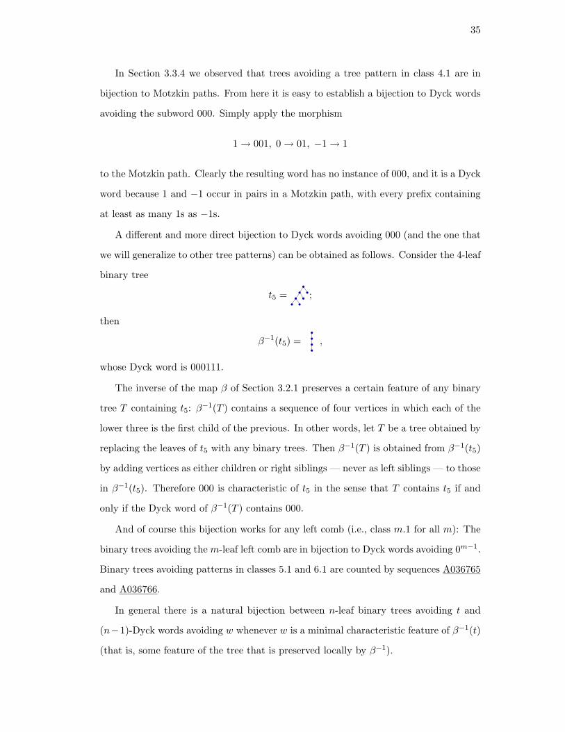
In Section 3.3.4 we observed that trees avoiding a tree pattern in class 4.1 are in

bijection to Motzkin paths. From here it is easy to establish a bijection to Dyck words

avoiding the subword 000. Simply apply the morphism

1→ 001, 0→ 01, −1→ 1

to the Motzkin path. Clearly the resulting word has no instance of 000, and it is a Dyck

word because 1 and −1 occur in pairs in a Motzkin path, with every prefix containing

at least as many 1s as −1s.

A different and more direct bijection to Dyck words avoiding 000 (and the one that

we will generalize to other tree patterns) can be obtained as follows. Consider the 4-leaf

binary tree

t5 = ;

then

β−1(t5) = ,

whose Dyck word is 000111.

The inverse of the map β of Section 3.2.1 preserves a certain feature of any binary

tree T containing t5: β−1(T ) contains a sequence of four vertices in which each of the

lower three is the first child of the previous. In other words, let T be a tree obtained by

replacing the leaves of t5 with any binary trees. Then β−1(T ) is obtained from β−1(t5)

by adding vertices as either children or right siblings — never as left siblings — to those

in β−1(t5). Therefore 000 is characteristic of t5 in the sense that T contains t5 if and

only if the Dyck word of β−1(T ) contains 000.

And of course this bijection works for any left comb (i.e., class m.1 for all m): The

binary trees avoiding the m-leaf left comb are in bijection to Dyck words avoiding 0m−1.

Binary trees avoiding patterns in classes 5.1 and 6.1 are counted by sequences A036765

and A036766.

In general there is a natural bijection between n-leaf binary trees avoiding t and

(n−1)-Dyck words avoiding w whenever w is a minimal characteristic feature of β−1(t)

(that is, some feature of the tree that is preserved locally by β−1).

36

For example, for the binary trees in class 4.2 we have

β−1

( )= , β−1

( )= , β−1

( )= .

Which of these patterns have a bijection to Dyck words? Consider the third tree,

= 001011.

While it is true that any tree containing this tree must contain 001, the converse is not

true, so this tree does not admit a bijection to Dyck words. However, the two trees

= 010011 and = 001101

contain the word 100 and its reverse complement 110 respectively, and containing one

of these subwords is a necessary and sufficient condition for the corresponding tree

to contain the respective tree pattern. Thus binary trees avoiding a tree pattern in

class 4.2 are in bijection to Dyck words avoiding 100, and they are counted by sequence

A011782.

Bijections for other patterns can be found similarly. Binary trees avoiding a tree

pattern in class 5.2 (sequence A086581) are in bijection to Dyck words avoiding 1100,

via

β−1

( )= .

Class 5.3 (sequence A005773) corresponds to 1000 via

β−1

( )= .

Class 6.3 corresponds to 11000 and class 6.6 to 10000 via

β−1

( )= and β−1

=

respectively.

It is apparent that results of this kind involve “two-pronged” trees because avoid-

ance for these trees corresponds to a local condition on Dyck words. It should not be

surprising then that not all equivalence classes of binary trees have a corresponding

Dyck word class. For example, classes 6.2, 6.4, 6.5, and 6.7 do not. The lack of a Dyck

37

word class can be proven in each case by exhibiting an n such that the number of n-leaf

binary trees avoiding t is not equal to the number of (n−1)-Dyck words avoiding w for

all w; only a finite amount of computation is required because all Cn−1 (n − 1)-Dyck

words avoid w for |w| > 2(n− 1). For example, n = 8 suffices for classes 6.2 and 6.5.

3.5 Algorithms

In this section we provide algorithms for computing algebraic equations satisfied by

Avt(x), EnL,t(x, y), and the more general EnL,p1,...,pk(xL, xp1 , . . . , xpk

) defined in Sec-

tion 3.5.3. Computing Avt(x) or EnL,t(x, y) for all m-leaf binary tree patters t allows

one to automatically determine the equivalence classes given in the appendix.

We draw upon the notation and results described in Section 3.2.2. In particular,

the intersection p ∩ p′ of two tree patterns plays a central role.

3.5.1 Avoiding a single tree

Fix a binary tree pattern t we wish to avoid. For a given tree pattern p, we will make

use of the generating function

weight(p) = weight(Lp) :=∑T∈Lp

weight(T ),

where

weight(T ) =

xnumber of vertices in T if T avoids t;

0 if T contains t.

The case t = L was covered in Section 3.3.1, so we assume t 6= L. Then t = (tltr)

for some tree patterns tl and tr. Since (TlTr) avoids t precisely when (Tl avoids t) and

(Tr avoids t) and ((Tl doesn’t match tl) or (Tr doesn’t match tr)), we have

weight((plpr)) =

x ·(weight(pl) · weight(pr)− weight(pl ∩ tl) · weight(pr ∩ tr)

). (3.1)

The coefficient x is the weight of the root vertex of (plpr) that we destroy in separating

this pattern into its two subpatterns.

38

We now construct a polynomial (with coefficients that are polynomials in x) that

is satisfied by Avt(x) = weight(L), the weight of the language of binary trees. The

algorithm is as follows.

Begin with the equation

weight(L) = weight(()) + weight((LL)).

The variable weight((LL)) is “new”; we haven’t yet written it in terms of other vari-

ables. So use Equation (3.1) to rewrite weight((LL)). For each expression weight(p ∩

p′) that is introduced, we compute the intersection p ∩ p′. This allows us to write

weight(p ∩ p′) as weight(q) for some pattern q that is simply a word on {(, ), L} (i.e.,

does not contain the ∩ operator).

For each new variable weight(q), obtain a new equation by making it the left side of

Equation (3.1), and then as before we eliminate ∩ by explicitly computing intersections.

We continue in this manner until there are no new variables produced. This must

happen because depth(p∩p′) ≤ max(depth(p), depth(p′)), so since there are only finitely

many trees that are shallower than t, there are only finitely many variables in this system

of polynomial equations.

Finally, compute a Grobner basis for the system in which all variables except

weight(()) = x and weight(L) = Avt(x) are eliminated. This gives a single poly-

nomial equation in these variables, which provides an algebraic equation satisfied by

Avt(x).

Let us work out an example. We use the graphical representation of tree patterns

with the understanding that the leaves are blanks. Consider the tree pattern

t = = (L(L((LL)L)))

from class 5.2. The first equation is

weight( ) = x+ weight( ).

We have tl = and tr = , so Equation (3.1) gives

weight( ) = x ·(weight( ) · weight( )− weight( ∩ ) · weight( ∩ )

)= x ·

(weight( )2 − weight( ) · weight( )

)

39

since L∩ p = p for any tree pattern p. The variable weight( ) = weight(tr) is new, so

we put it into Equation (3.1):

weight( ) = x ·(weight( ) · weight( )− weight( ∩ ) · weight( ∩ )

)= x ·

(weight( ) · weight( )− weight( ) · weight( )

).

There are two new variables:

weight( ) = x ·(weight( ) · weight( )− weight( ∩ ) · weight( ∩ )

)= x ·

(weight( ) · weight( )− weight( ) · weight( )

);

weight( ) = x ·(weight( ) · weight( )− weight( ∩ ) · weight( ∩ )

)= x ·

(weight( ) · weight( )− weight( ) · weight( )

).

We have no new variables, so we eliminate the four auxiliary variables

weight( ),weight( ),weight( ),weight( )

from this system of five equations to obtain

x3 weight( )2 − (x2 − 1)2 weight( )− x (x2 − 1) = 0.

3.5.2 Enumerating with respect to a single tree

To prove Theorem 3.1, we make a few modifications in order to compute EnL,t(x, y)

instead of Avt(x). Again

weight(p) :=∑T∈Lp

weight(T ),

but now weight(T ) = xnumber of vertices in T ynumber of copies of t in T for all T . We modify

Equation (3.1) to become

weight((plpr)) =

x ·(weight(pl) · weight(pr) + (y − 1) · weight(pl ∩ tl) · weight(pr ∩ tr)

)(3.2)

since in addition to accounting for the trees that avoid t we also account for those that

match t, in which case y is contributed.

The rest of the algorithm carries over unchanged, and we obtain a polynomial equa-

tion in x, y, and EnL,t(x, y) = weight(L).

40

3.5.3 Enumerating with respect to multiple trees

A more general question is the following. Given several binary tree patterns p1, . . . , pk,

what is the number an0,n1,...,nkof binary trees containing precisely n0 vertices, n1 copies

of p1, . . . , nk copies of pk? We consider the enumerating generating function

EnL,p1,...,pk(xL, xp1 , . . . , xpk

) =∑T

xα0L x

α1p1 · · ·x

αkpk

=∞∑

n0=0

∞∑n1=0

· · ·∞∑

nk=0

an0,n1,...,nkxn0L x

n1p1 · · ·x

nkpk,

where p0 = L and αi is the number of copies of pi in T . (We need not assume that

the pi are distinct.) This generating function can be used to obtain information about

how correlated a family of tree patterns is. We have the following generalization of

Theorem 3.1.

Theorem 3.3. EnL,p1,...,pk(xL, xp1 , . . . , xpk

) is algebraic.

Keeping track of multiple tree patterns p1, . . . , pk is not much more complicated

than handling a single pattern, and the algorithm for doing so has the same outline.

Let

weight(p) :=∑T∈Lp

weight(T )

with

weight(T ) = xnLxα1p1 · · ·x

αkpk,

where αi is the number of copies of pi in T . Let d = max1≤i≤k depth(pi). First

we describe what to do with each new variable weight(q) that arises. The approach

used is different than that for one tree pattern; in particular, we do not make use of

intersections. Consequently, it is less efficient.

Let l be the number of leaves in q. If T is a tree matching q, then for each leaf L

of q there are two possibilities: Either L is matched by a terminal vertex () in T , or L

is matched by a tree matching (LL). For each leaf we make this choice independently,

thus partitioning the language Lq into 2l disjoint sets represented by 2l tree patterns

that are disjoint in the sense that each tree matching q matches precisely one of these

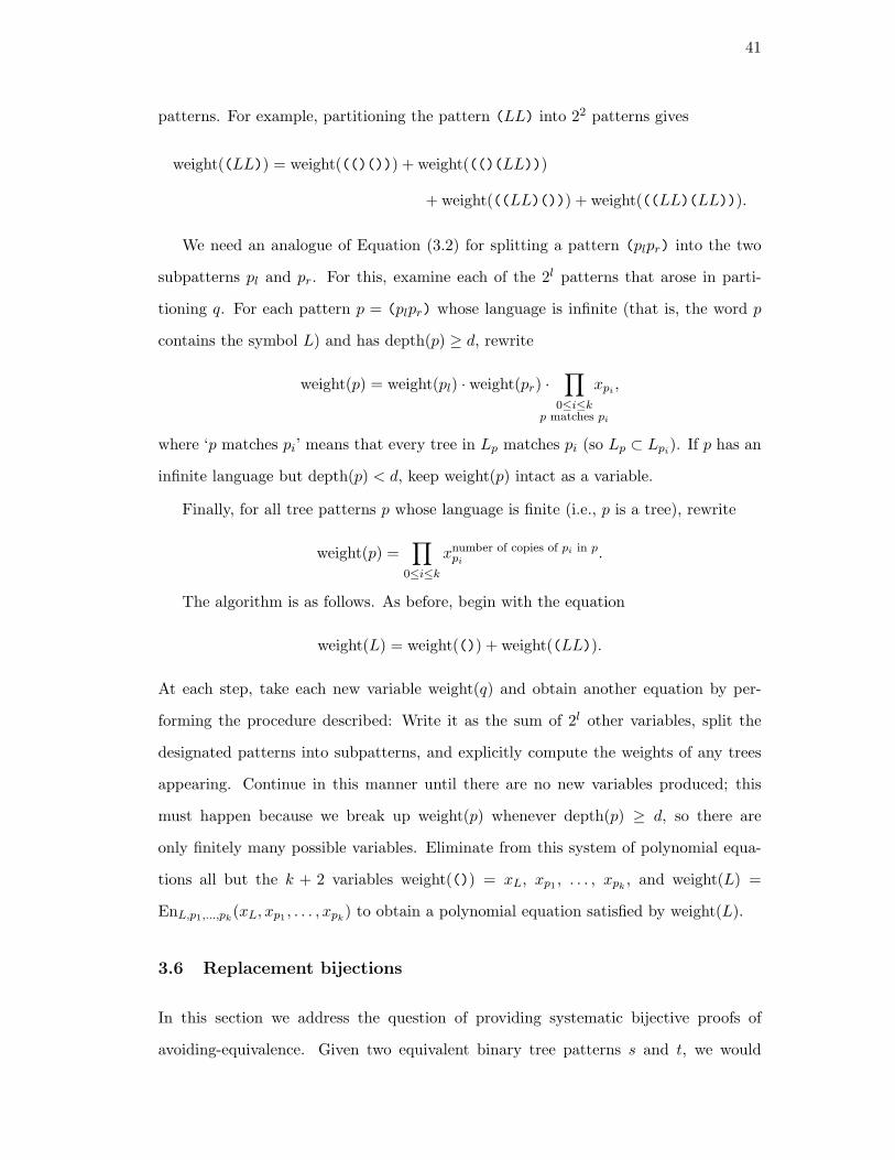
41

patterns. For example, partitioning the pattern (LL) into 22 patterns gives

weight((LL)) = weight((()())) + weight((()(LL)))

+ weight(((LL)())) + weight(((LL)(LL))).

We need an analogue of Equation (3.2) for splitting a pattern (plpr) into the two

subpatterns pl and pr. For this, examine each of the 2l patterns that arose in parti-

tioning q. For each pattern p = (plpr) whose language is infinite (that is, the word p

contains the symbol L) and has depth(p) ≥ d, rewrite

weight(p) = weight(pl) · weight(pr) ·∏

0≤i≤kp matches pi

xpi ,

where ‘p matches pi’ means that every tree in Lp matches pi (so Lp ⊂ Lpi). If p has an

infinite language but depth(p) < d, keep weight(p) intact as a variable.

Finally, for all tree patterns p whose language is finite (i.e., p is a tree), rewrite

weight(p) =∏

0≤i≤kxnumber of copies of pi in ppi

.

The algorithm is as follows. As before, begin with the equation

weight(L) = weight(()) + weight((LL)).

At each step, take each new variable weight(q) and obtain another equation by per-

forming the procedure described: Write it as the sum of 2l other variables, split the

designated patterns into subpatterns, and explicitly compute the weights of any trees

appearing. Continue in this manner until there are no new variables produced; this

must happen because we break up weight(p) whenever depth(p) ≥ d, so there are

only finitely many possible variables. Eliminate from this system of polynomial equa-

tions all but the k + 2 variables weight(()) = xL, xp1 , . . . , xpk, and weight(L) =

EnL,p1,...,pk(xL, xp1 , . . . , xpk

) to obtain a polynomial equation satisfied by weight(L).

3.6 Replacement bijections

In this section we address the question of providing systematic bijective proofs of

avoiding-equivalence. Given two equivalent binary tree patterns s and t, we would

42

like to produce an explicit bijection between binary trees avoiding s and binary trees

avoiding t. It turns out that this can often be achieved by structural replacements on

trees. We start by describing an example in full, and later generalize.

3.6.1 An example replacement bijection

Consider the trees

t2 = and t3 =

in class 4.2. The idea is that since n-leaf trees avoiding t2 are in bijection to n-leaf

trees avoiding t3, then somehow swapping all occurrences of these tree patterns should

produce a bijection. However, since the patterns may overlap, it is necessary to specify

an order in which to perform the replacements. A natural order is to start with the

root and work down the tree. More precisely, a top-down replacement is a restructuring

of a tree T in which we iteratively apply a set of transformation rules to subtrees of T ,

working downward from the root.

Take the replacement rule to be

a b c d→ c

a bd,

where the variables represent trees attached at the leaves, rearranged according to the

permutation 3124. (Most permutations are not viable; we discuss this in the next

section.) Begin at the root: If T itself matches the left side of the rule, then we

restructure T according to the rule; if not, we leave T unchanged. Then we repeat the

procedure on the root’s (new) children, then on their children, etc., so that each vertex

in the tree is taken to be the root of a subtree which is possibly transformed by the

rule. For example,

→ → →

shows the three replacements required to compute the image (on the right) of the left

tree via two intermediate trees.

43

This top-down replacement is invertible. The inverse map is a bottom-up replacement

with the inverse replacement rule,

a

b cd→

b c a d.

Rather than starting at the root and working down the tree, start at the leaves and

work up the tree.

We now show that the top-down replacement is in fact a bijection from trees avoiding

t2 to trees avoiding t3. It turns out to be the same bijection given in Section 3.3.4 via

words in {0, 1}n−2.

Assume T avoids t2; we show that the image of T under the top-down replacement

avoids t3. It is helpful to think of T as broken up into (possibly overlapping) “spheres

of influence” — subtrees which are maximal with respect to the replacement rule in

the sense that performing the top-down replacement on the subtree does not introduce

instances of the relevant tree patterns containing vertices outside of the subtree. It

suffices to consider each sphere of influence separately. A natural focal point for each

sphere of influence is the highest occurrence of t3. We verify that restructuring this t3

to t2 under the top-down replacement produces no t3 above, at, or below the root of

the new t2 in the image of T .

above: Since t3 has depth 2, t3 can occur at most one level above the root of the new t2

while overlapping it. Thus it suffices to consider all subtrees with t3 occurring at

level 1. There are two cases,

e

a b c d

anda b c d

e .

The first case does not avoid t2, so it does not occur in T . The second case may

occur in T . However, we do not want the subtree itself to match t3 (because we

assume that the t3 at level 1 is the highest t3 in this sphere of influence), so we

must have e = (). Thus this subtree is transformed by the top-down replacement

as

a b c d

→ c

a bd.

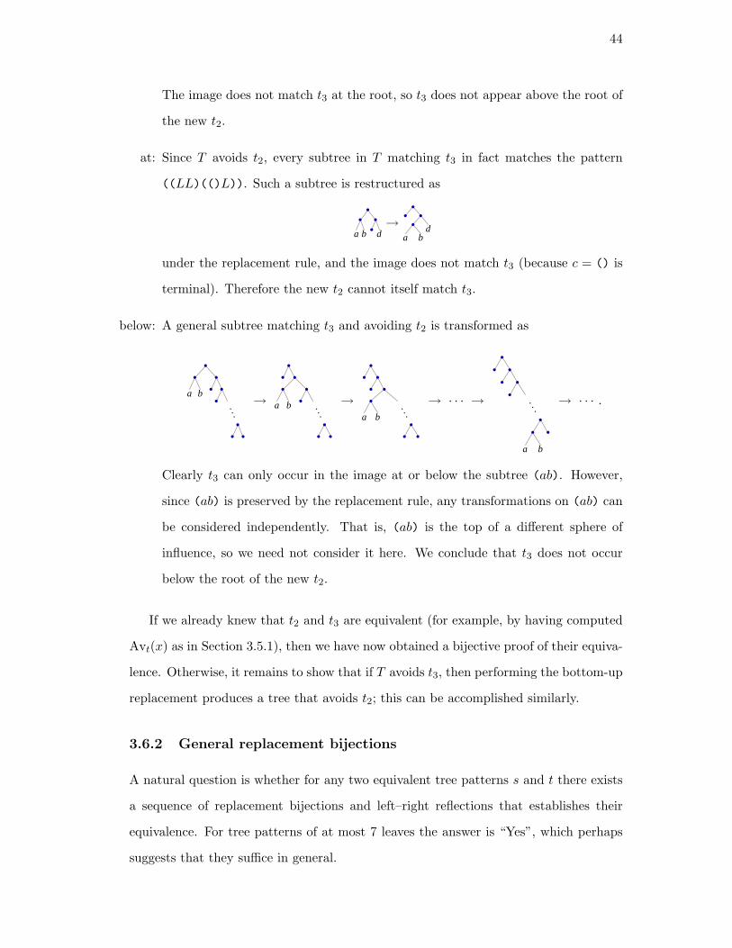
44

The image does not match t3 at the root, so t3 does not appear above the root of

the new t2.

at: Since T avoids t2, every subtree in T matching t3 in fact matches the pattern

((LL)(()L)). Such a subtree is restructured as

a b d→

a bd

under the replacement rule, and the image does not match t3 (because c = () is

terminal). Therefore the new t2 cannot itself match t3.

below: A general subtree matching t3 and avoiding t2 is transformed as

a b → a b →a b

→ · · · →

a b

→ · · · .

Clearly t3 can only occur in the image at or below the subtree (ab). However,

since (ab) is preserved by the replacement rule, any transformations on (ab) can

be considered independently. That is, (ab) is the top of a different sphere of

influence, so we need not consider it here. We conclude that t3 does not occur

below the root of the new t2.

If we already knew that t2 and t3 are equivalent (for example, by having computed

Avt(x) as in Section 3.5.1), then we have now obtained a bijective proof of their equiva-

lence. Otherwise, it remains to show that if T avoids t3, then performing the bottom-up

replacement produces a tree that avoids t2; this can be accomplished similarly.

3.6.2 General replacement bijections

A natural question is whether for any two equivalent tree patterns s and t there exists

a sequence of replacement bijections and left–right reflections that establishes their

equivalence. For tree patterns of at most 7 leaves the answer is “Yes”, which perhaps

suggests that they suffice in general.

45

Conjecture 3.4. Two binary tree patterns s and t are equivalent if and only if there is

a sequence of top-down replacements, bottom-up replacements, and left–right reflections

that produces a bijection from binary trees avoiding s to binary trees avoiding t.

In this section we discuss qualitative results regarding this conjecture.

Given two m-leaf tree patterns s and t, one can ask which permutations of the

leaves give rise to a top-down replacement that induces a bijection from trees avoiding

s to trees avoiding t. Candidate permutations can be found experimentally by simply

testing all m! permutations of leaves on a set of randomly chosen binary trees avoiding

s; one checks that the image avoids t and that composing the top-down replacement

with the inverse bottom-up replacement produces the original tree. This approach is

feasible for small m, but it is slow and does not provide any insight into why certain

trees are equivalent. A question unresolved at present is to efficiently find all such

bijections. The naive method was used to find the examples in this section.

Once a candidate bijection is found, it can be proved in a manner similar to Sec-

tion 3.6.1. Although we do not attempt here to fully generalize that argument, the

following two examples provide an indication of the issues encountered in the ‘above’

and ‘below’ cases of the general setting.

As an example of what can go wrong in the ‘above’ case, consider the replacement

rule

a

b cd→

b c a d

given by the permutation 2314 on 4-leaf binary trees s = t3 and t = t2. This rule does

not induce a top-down replacement bijection from trees avoiding t3 to trees avoiding

t2. One obstruction is the mapping

→ .

The initial tree avoids t3. However, it contains t2, and replacing this t2 with t3 completes

another t2. The final tree does not avoid t2.

In general, for the ‘above’ case it suffices to check all trees avoiding s of a certain

depth where the highest t begins at level depth(t) − 1. A bound on the depth is

46

possible since for a given set of replacement rules there is a maximum depth at which

the structure of a subtree can affect the top depth(t) + 1 levels of the image. If,

after performing the top-down replacement on these trees, no t appears above level

depth(t)− 1, then t can never appear above the root of the highest t in the subtree.

An example of what can go wrong in the ‘below’ case is provided by the rule

a

b cd→ a

db c

given by the permutation 1423 on 4-leaf binary trees s = t1 and t = t2. This rule does

not induce a top-down replacement bijection from trees avoiding t1 to trees avoiding

t2. (Indeed, these trees are not equivalent.) One obstruction is the mapping

→ → .

The initial tree avoids t1. However, it matches t2, and replacing this t2 with t1 produces

a copy of the intersection t1 ∩ t2 in the intermediate step. The t2 is then replaced by

t1, but this does not change the tree because t1 ∩ t2 is fixed by the rule. Therefore the

final tree does not avoid t2.

A general proof for the ‘below’ case must take into account all ways of producing,

below the root of the highest t in a subtree, a copy t of that is not broken by further

replacements.

We now return briefly to the replacement rule of Section 3.6.1 to mention that a

minor modification produces a bijection on the full set of binary trees. Namely, take

the two replacement rules

a b c d→ c

a bd

and a

b cd→

b c a d.

Again we perform a top-down replacement, now using both rules together. That is, if

a subtree matches the left side of either rule, we restructure it according to that rule.

Of course, it can happen that a particular subtree matches both replacement rules,

resulting in potential ambiguity; in this case which do we apply? Well, if both rules

result in the same transformation, then it does not matter, and indeed with our present

example this is the case. To show this, it suffices to take the intersection t2 ∩ t3 of the

47

two left sides and label the leaves to represent additional branches that may be present:

p1 p2

p3 p4

p5.

Now we check that applying each of the two replacement rules to this tree produces the

same labeled tree, namely

p3 p4

p1 p2

p5.

Therefore we need not concern ourselves with which rule is applied to a given subtree

that matches both. Since the replacement rules agree on their intersection, the top-

down replacement is again invertible and is therefore a bijection from the set of binary

trees to itself. By the examination of cases in the previous section, this bijection is an

extension of the bijection between binary trees avoiding t2 and binary trees avoiding t3.

Thus we may choose from two types of bijection when searching for top-down re-

placement bijections that prove avoiding-equivalence. The first type is from binary

trees avoiding s to binary trees avoiding t, using one rule for the top-down direction

and the inverse for the bottom-up direction; these bijections in general do not extend

to bijections on the full set of binary trees. The second type is a bijection on the full set

of binary trees, using both rules in each direction, that induces a bijection from binary

trees avoiding s to binary trees avoiding t.

Empirically, each two-rule bijection that proves avoiding-equivalence for s and t

induces a one-rule bijection proving this equivalence, as in the previous example. How-

ever, not all two-rule bijections, when restricted to one rule, become bijections that

prove avoiding-equivalence; the rules used to discuss the ‘above’ and ‘below’ cases in

this section are two counterexamples.

One benefit to searching for two-rule bijections is that requiring the two replacement

rules to agree on the leaf-labeled intersection s ∩ t quickly prunes the set of candidate

permutations. There is a tradeoff, however, because verifying a two-rule bijection is

more complicated than verifying a one-rule bijection.

Searching for two-rule bijections on 4-leaf binary tree patterns, one finds only the

rules given by the permutation 3124 for s = t2 and t = t3, mentioned above, and their

48

t2 t3 t4 t6 t7 t8 t9 t11 t12 t13

t2 — 14235 43125t3 — 12534 31245 51234t4 12453 — 41235t6 — 12534 45123t7 12453 — 45123t8 34512 — 31245t9 34512 23145 —t11 13452 — 31245t12 23451 12453 23145 —t13 14532 13425 —

Table 3.1: Leaf permutations whose two-rule replacements prove avoiding-equivalencefor pairs of trees in class 5.2.

left–right reflections, given by 1342 for s = t4 and t = t3. (Note the asymmetry here:

There is a top-down replacement bijection from trees avoiding t2 to trees avoiding t3

but not vice versa.)

However, this does not account for all top-down replacement bijections for these

patterns. The permutation 3142 for s = t2 and t = t3 and its left–right reflection 3142

for s = t4 and t = t3 provide one-rule bijections that do not extend to all binary trees.

Among equivalence classes of 5-leaf binary tree patterns, class 5.2 is the only class

containing nontrivial equivalences. It consists of the ten trees t2, t3, t4, t6, t7, t8, t9,

t11, t12, and t13, pictured as follows.

For each pair of trees in this class, Table 3.1 lists the leaf permutations that prove

equivalence by a two-rule top-down replacement. It happens that there is at most one

permutation for each pair in this class, although in general there may be more.

With this data, one might suspect that two-rule replacement bijections are sufficient

to establish every equivalence class of binary tree patterns. In fact they are not. The

smallest counterexample is class 7.15, which consists of the three trees

t61 = , t65 = , and t81 =

49

and their left–right reflections. Trees t81 and t61 are equivalent by the permutation

1456723, but no permutation of leaves produces a two-rule replacement bijection that

establishes the equivalence of t65 to one of the others. However, the permutations

4561237 and 4571236 provide candidate one-rule bijections for t65 and t61, and 2341675

provides a candidate bijection for t65 and t81.

We conclude with a curious example in which two tree patterns can only be proven

equivalent by a two-rule bijection that does not involve them directly. The trees

t7 = and t11 =

in class 6.5 are avoiding-equivalent by the permutation 126345, but neither

t17 =

nor its left–right reflection has an equivalence-proving permutation to t7, t11, or their

left–right reflections. Thus, this equivalence cannot be established by a bijection that

swaps 6-leaf tree patterns. However, it can be established by a bijection that swaps 4-

leaf tree patterns: The previously mentioned bijection consisting of the two replacement

rules

a b c d→ c

a bd

and a

b cd→

b c a d,

induces a top-down replacement bijection from trees avoiding t7 to trees avoiding t17.

The reason is that t7 and t17 are formed by two overlapping copies of the class 4.2 trees

and

respectively, and that t7 and t17 are mapped to each other under this bijection.

50

Appendix. Table of equivalence classes

Here we list equivalence classes of binary trees with at most 7 leaves. Left–right reflec-

tions are omitted for compactness. For each class we provide a polynomial equation

satisfied by f = EnL,t(x, y); an equation satisfied by Avt(x) is obtained in each case by

letting y = 0. These equations were computed in Mathematica and Singular using the

packages TreePatterns [27] and Singular [18]. TreePatterns contains additional

pre-computed data extended to 8-leaf binary trees. The number of equivalence classes

of m-leaf binary trees for m = 1, 2, 3, . . . is 1, 1, 1, 2, 3, 7, 15, 44, . . . .

Class 1.1 (1 tree)

xyf2 − f + xy = 0

Class 2.1 (1 tree)

xyf2 − f + x = 0

Class 3.1 (2 trees)

xyf2 +(−x2(y − 1)− 1

)f + x = 0

Class 4.1 (2 trees)

(xy − x3(y − 1)

)f2 +

(−x2(y − 1)− 1

)f + x = 0

51

Class 4.2 (3 trees)

xyf2 +(−2x2(y − 1)− 1

)f +

(x3(y − 1) + x

)= 0

Class 5.1 (2 trees)

−x4(y − 1)f3 +(xy − x3(y − 1)

)f2 +

(−x2(y − 1)− 1

)f + x = 0

Class 5.2 (10 trees)

(xy − x3(y − 1)

)f2 +

(x2 (x2 − 2

)(y − 1)− 1

)f +

(x3(y − 1) + x

)= 0

Class 5.3 (2 trees)

xyf3 +(−3x2(y − 1)− 1

)f2 +

(3x3(y − 1) + x

)f − x4(y − 1) = 0

Class 6.1 (2 trees)

−x5(y − 1)f4 − x4(y − 1)f3 +(xy − x3(y − 1)

)f2 +

(−x2(y − 1)− 1

)f + x = 0

Class 6.2 (8 trees)

−x4(y − 1)f3 + x(x2 (x2 − 1

)(y − 1) + y

)f2 +

(x2 (x2 − 2

)(y − 1)− 1

)f +

(x3(y − 1) + x

)= 0

52

Class 6.3 (14 trees)

x(x2 (x2 − 2

)(y − 1) + y

)f2 +

(2x2 (x2 − 1

)(y − 1)− 1

)f +

(x3(y − 1) + x

)= 0

Class 6.4 (8 trees)

(xy − x3(y − 1)

)f3 +

(x2 (2x2 − 3

)(y − 1)− 1

)f2

+(−x5(y − 1) + 3x3(y − 1) + x

)f − x4(y − 1) = 0

Class 6.5 (6 trees)

(xy − 2x3(y − 1)

)f2 +

(x2 (3x2 − 2

)(y − 1)− 1

)f +

(−x5(y − 1) + x3(y − 1) + x

)= 0

Class 6.6 (2 trees)

−xyf4 +(4x2(y − 1) + 1

)f3 +

(−6x3(y − 1)− x

)f2 + 4x4(y − 1)f − x5(y − 1) = 0

Class 6.7 (2 trees)

x4 (x2(y − 1)− y)

(y − 1)f3 +(−2x7(y − 1)2 + x5(y − 1)(3y − 2)− x3(y − 1) + xy

)f2

+(x2 (x6(y − 1)− 3x4(y − 1) + x2 − 2

)(y − 1)− 1

)f +

(x7(y − 1)2 + x3(y − 1) + x

)= 0

53

Class 7.1 (2 trees)

−x6(y − 1)f5 − x5(y − 1)f4 − x4(y − 1)f3 +(xy − x3(y − 1)

)f2 +

(−x2(y − 1)− 1

)f + x = 0

Class 7.2 (10 trees)

− x5(y − 1)f4 + x4 (x2 − 1)

(y − 1)f3

+ x((

x2 − 1)x2(y − 1) + y

)f2 +

(x2 (x2 − 2

)(y − 1)− 1

)f +

(x3(y − 1) + x

)= 0

Class 7.3 (20 trees)

x4 (x2 − 1)

(y − 1)f3 + x(2(x2 − 1

)x2(y − 1) + y

)f2

+(2x2 (x2 − 1

)(y − 1)− 1

)f +

(x3(y − 1) + x

)= 0

Class 7.4 (6 trees)

− x4(y − 1)f4 + x((

2x2 − 1)x2(y − 1) + y

)f3

+(−(x4 − 2x2 + 3

)x2(y − 1)− 1

)f2 +

(−x5(y − 1) + 3x3(y − 1) + x

)f − x4(y − 1) = 0

54

Class 7.5 (10 trees)

− x4(y − 1)f3 + x(2(x2 − 1

)x2(y − 1) + y

)f2

+(−(x4 − 3x2 + 2

)x2(y − 1)− 1

)f +

(−x5(y − 1) + x3(y − 1) + x

)= 0

Class 7.6 (16 trees)

x((

x2 − 2)x2(y − 1) + y

)f3 +

(−(x4 − 4x2 + 3

)x2(y − 1)− 1

)f2

+(−2x5(y − 1) + 3x3(y − 1) + x

)f − x4(y − 1) = 0

Class 7.7 (10 trees)

(x3(y − 1)− xy

)f4 +

(1− x2 (3x2 − 4

)(y − 1)

)f3

+ x(3x2 (x2 − 2

)(y − 1)− 1

)f2 − x4 (x2 − 4

)(y − 1)f − x5(y − 1) = 0

Class 7.8 (4 trees)

x4(y − 1)(2x2(y − 1)− y − 1

)f3 +

(−5x7(y − 1)2 + 3x5(y − 1)y − x3(y − 1) + xy

)f2

+(x2(y − 1)

(4x6(y − 1) + x4(2− 3y) + x2 − 2

)− 1)f

− x(x4(y − 1) + 1

) (x2 (x2 − 1

)(y − 1)− 1

)= 0

55

Class 7.9 (20 trees)

x((

2x2 − 3)x2(y − 1) + y

)f2

+(−(x4 − 4x2 + 2

)x2(y − 1)− 1

)f +

(−x5(y − 1) + x3(y − 1) + x

)= 0

Class 7.10 (10 trees)

(xy − 2x3(y − 1)

)f3 +

(x2 (5x2 − 3

)(y − 1)− 1

)f2

+(−4x5(y − 1) + 3x3(y − 1) + x

)f + x4 (x2 − 1

)(y − 1) = 0

Class 7.11 (6 trees)

(x(x2 − 1

)3y − x3 (x4 − 3x2 + 3

))f3 +

(x2 (3 (x2 − 2

)x2(y − 1) + 3y − 2

)+ 1)f2

+ x(3x2 (x2 − 1

)(y − 1)− 2

)f +

(x4(y − 1) + x2) = 0

Class 7.12 (2 trees)

xyf5 +(−5x2(y − 1)− 1

)f4 +

(10x3(y − 1) + x

)f3 − 10x4(y − 1)f2 + 5x5(y − 1)f − x6(y − 1) = 0

56

Class 7.13 (2 trees)

− x10(y − 1)3(x2(y − 1)− y

)f5 + x5(y − 1)

(4x8(y − 1)3 − x6(y − 1)2(5y − 2) + x2(y − 1)(2y − 1)− y2

)f4

− x4(y − 1)(6x10(y − 1)3 − x8(y − 1)2(10y − 7) + x4(y − 1)(7y − 5) + x2(3− 4y)y − y + 1

)f3

+ x(x2(y − 1)

(x2(y − 1)

(x2(x2(x4(y − 1)

(4x2(y − 1)− 10y + 9

)+ 9y − 8

)− 6y + 2

)− 3

)− 2

)+ y

)f2

+(−x2(y − 1)

(x2(x2(y − 1)

(x2(x2(y − 1)

((x2 − 5

)x4(y − 1) + 5

)− 4y + 3

)− 3

)− 3

)+ 2

)− 1

)f

− x(x2(y − 1)

(x12(y − 1)3 − x8(y − 1)2 + x6(y − 1)2 + x4(y − 1) + x2 − 1

)− 1

)= 0

Class 7.14 (8 trees)

(x− 1)x4(x + 1)(y − 1)((

x2 − 2)x2(y − 1) + y

)f3

+ x((x− 1)(x + 1)x2(y − 1)

(3(x2 − 1

)x2(y − 1) + 2

)+ y)f2

+((x− 1)x2(x + 1)(y − 1)

(3x4(y − 1) + 2

)− 1)f +

(x7(y − 1)2 + x3(y − 1) + x

)= 0

Class 7.15 (6 trees)

x6(y − 1)f3 + x((

x2 − 3)x2(y − 1) + y

)f2

+(2x2 (2x2 − 1

)(y − 1)− 1

)f +

(−x5(y − 1) + x3(y − 1) + x

)= 0

57

References

[1] Jean-Paul Allouche and Jeffrey Shallit, The ring of k-regular sequences, TheoreticalComputer Science 98 (1992) 163–197.

[2] Jonathan Borwein et al., Inverse Symbolic Calculator, http://glooscap.cs.dal.ca.

[3] Nicolaas de Bruijn and B. J. M. Morselt, A note on plane trees, Journal of Com-binatorial Theory 2 (1967) 27–34.

[4] Benoit Cloitre, Beyond Rowland’s gcd sequence, preprint.

[5] Emeric Deutsch, Dyck path enumeration, Discrete Mathematics 204 (1999) 167–202.

[6] Robert Donaghey and Louis Shapiro, Motzkin numbers, Journal of CombinatorialTheory, Series A 23 (1977) 291–301.

[7] Underwood Dudley, History of a formula for primes, The American MathematicalMonthly 76 (1969) 23–28.

[8] Philippe Flajolet and Robert Sedgewick, Analytic Combinatorics, Cambridge Uni-versity Press, 2009.

[9] Philippe Flajolet, Paolo Sipala, and Jean-Marc Steyaert, Analytic variations on thecommon subexpression problem, Lecture Notes in Computer Science: Automata,Languages, and Programming 443 (1990) 220–234.

[10] Matthew Frank, personal communication, July 15, 2003.

[11] J. M. Gandhi, Formulae for the nth prime, Proceedings of the Washington StateUniversity Conference on Number Theory 96–107, Washington State University,Pullman, WA, 1971.

[12] Solomon Golomb, A direct interpretation of Gandhi’s formula, The AmericanMathematical Monthly 81 (1974) 752–754.

[13] R. L. Goodstein and C. P. Wormell, Formulae for primes, The MathematicalGazette 51 (1967) 35–38.

[14] Ian Goulden and David Jackson, An inversion theorem for cluster decompositionsof sequences with distinguished subsequences, Journal of the London MathematicalSociety (second series) 20 (1979) 567–576.

[15] Frank Harary, Geert Prins, and William Tutte, The number of plane trees, Inda-gationes Mathematicae 26 (1964) 319–329.

58

[16] James Jones, Formula for the nth prime number, Canadian Mathematical Bulletin18 (1975) 433–434.

[17] James Jones, Daihachiro Sato, Hideo Wada, and Douglas Wiens, Diophantinerepresentation of the set of prime numbers, The American Mathematical Monthly83 (1976) 449–464.

[18] Manuel Kauers and Viktor Levandovskyy, Singular [a Mathematica pack-age], available from http://www.risc.uni-linz.ac.at/research/combinat/software/Singular/.

[19] Donald Knuth, The Art of Computer Programming, second edition, Volume 1:Fundamental Algorithms, Addison–Wesley, 1973.

[20] Yuri Matiyasevich, Diophantine representation of the set of prime numbers (inRussian), Doklady Akademii Nauk SSSR 196 (1971) 770–773. English translationby R. N. Goss, in Soviet Mathematics 12 (1971) 249–254.

[21] William Mills, A prime-representing function, Bulletin of the American Mathemat-ical Society 53 (1947) 604.

[22] John Noonan and Doron Zeilberger, The Goulden–Jackson cluster method: ex-tensions, applications, and implementations, Journal of Difference Equations andApplications 5 (1999) 355–377.

[23] Simon Plouffe, Plouffe’s Inverter, http://pi.lacim.uqam.ca.

[24] Paulo Ribenboim, The New Book of Prime Number Records, third edition,Springer–Verlag New York Inc., 1996.

[25] Eric Rowland, A natural prime-generating recurrence, Journal of Integer Sequences11 (2008) 08.2.8.

[26] Eric Rowland, Pattern avoidance in binary trees, preprint.

[27] Eric Rowland, TreePatterns [a Mathematica package], available from http://math.rutgers.edu/~erowland/programs.html.

[28] Aris Sapounakis, Ioannis Tasoulas, and Panos Tsikouras, Counting strings in Dyckpaths, Discrete Mathematics 307 (2007) 2909–2924.

[29] Neil Sloane, The On-Line Encyclopedia of Integer Sequences, http://www.research.att.com/~njas/sequences (sequences A001006, A005773, A011782,A036765, A036766, A084662, A084663, A086581, A106108, A132199, A134162,A135506, and A137613).

[30] Jean-Marc Steyaert and Philippe Flajolet, Patterns and pattern-matching in trees:an analysis, Information and Control 58 (1983) 19–58.

[31] C. P. Willans, On formulae for the nth prime number, The Mathematical Gazette48 (1964) 413–415.

[32] Stephen Wolfram, A New Kind of Science, Wolfram Media, Inc., Champaign, IL,2002.

59

[33] Doron Zeilberger, An enquiry concerning human (and computer!) [mathemati-cal] understanding, Randomness & Complexity, from Leibniz to Chaitin (CristianCalude, ed.), World Scientific, Singapore, 2007.

60

Vita

Eric Rowland

2009 Ph.D. in Mathematics, Rutgers University

2003 B.A. in Mathematics, University of California Santa Cruz

2000 Graduated from Clark High School, Las Vegas, NV.

2009 Graduate assistant, Department of Mathematics, Rutgers University

2005–2008 Teaching assistant, Department of Mathematics, Rutgers University

2003–2005 Henry C. Torrey graduate assistant, Department of Mathematics, RutgersUniversity