experimental piezoelectric system identification
TRANSCRIPT

Journal of Mechanical Engineering and Automation 2017, 7(6): 179-195
DOI: 10.5923/j.jmea.20170706.01
Experimental Piezoelectric System Identification
Timothy Sands*, Tom Kenny
Department of Mechanical Engineering, Stanford University, USA
Abstract In this research article, you will learn about experimental system identification of natural frequencies of
vibration of a piezoelectric film element including a detailed introduction to several factors that often confound application
of theories to the real world: 1) additional response data induced by signal measurement, 2) signal harmonics, and 3)
signals induced by the power supply. Signals are read and processed from a piezoelectric element configured as a cantilever,
which is bent by a motor and cam assembly. Due to the piezoelectric effect, the strain created by the mechanical
displacement generates charges in the piezoelectric material, which is translated to a voltage reading with a charge
amplifier circuit. The effects of reference resistance and capacitance and the time constant of the circuit were investigated
using a National Instruments myDAQ. The myDAQ oscilloscope effectively displayed time response, but spectral data was
suspect. Especially since system identification (ID) largely comprises identification of the natural frequency, it is preferred
to not modify the signal being measured (as is the case with the oscilloscope). Furthermore, improved spectral plots were
seen with increased supply voltage (not always a good thing); therefore buffers were investigated next. The buffer provided
improved spectral data, but the buffer output did whatever was necessary to the signal to make the voltages at the inputs be
equal (again, modifying the signal). Using op-amps in the buffer configuration resulted in pretty spectral plots, but
contained “ghost” resonances, while using the op-amps in a two-stage charge amplifier configuration suppressed the “ghost
resonances”. In all cases, taking measurements at the output of the charge amplifier was superior to taking measurements at
the voltage amplifier. A two-stage amplification configuration provided on-the-order-of triple voltage signal (peak minus
offset) amplification. Several of the cases investigated provided good signal amplification with very legible spectral data
plots.
Keywords Piezoelectric, System identification, Cantilever, National Instruments, myDAQ, op-amp, Buffer, Spectral
data, Signal measurement, Harmonics, Power supply frequencies
1. Introduction
1.1. Background
The purpose of this research includes using a National
Instruments [1, 9] myDAQ [2] to read and process signals
from a piezoelectric film element [3, 10]. See Figure 1. The
goal of the paper is to stand as an easy-to-follow guide to
experimental system identification with many illustrations
to help investigators duplicate the procedure and results. A
piezoelectric element is configured as a cantilever [4],
which is bent by a motor and cam assembly [5]. Due to the
piezoelectric effect, the strain created by the mechanical
displacement [6] generates charges in the piezoelectric
material, which are translated to a voltage reading with a
charge amplifier circuit [7]. This article takes the reader
through a rigorously documented procedure to duplicate
* Corresponding author:
[email protected] (Timothy Sands)
Published online at http://journal.sapub.org/jmea
© 2017 The Author(s). Published by Scientific & Academic Publishing
This work is licensed under the Creative Commons Attribution International
License (CC BY). http://creativecommons.org/licenses/by/4.0/
experiments that distinguish real data from other factors that
often confound theorist seeking to apply their knowledge
experimentally: 1) additional response data induced by
signal measurement, 2) signal harmonics, and 3) signals
induced by the power supply. We’ll start by investigating
the effect of Rref, Cref (reference resistance and
capacitance respectively) and the time constant of the
intended circuit [8].
1.2. Literature Review
Space radar structures [11] utilize smart structural control
of lightweight spacecraft using piezoelectric elements begin
with controlling the rigid body dynamics (equation (1) in
[13]) that are disturbed by rotating attitude control actuators
[12, 13, 15, 17, 20, 25, 27]. Especially to avoid
control-structural interaction, flexible appendages and
robotic manipulators are included by adding the flexible
dynamics to the rigid body dynamics. In order to account
for imprecise estimates of the dynamic properties, nonlinear
adaptive controllers are a logical next step [13, 16, 19,
21-24, 26, 28-32] that include online system identification
algorithms [30-32]. These algorithms perform ubiquitously
better when initialized by good estimates of system

180 Timothy Sands et al.: Experimental Piezoelectric System Identification
parameters, making a priori system identification very
important. Taken together, these methods provide effective
control of lightweight, flexible space structures with fine
pointing supporting wide-array radar employment [11, 14,
18] or optical imaging.
1.3. Formulation of the Problem of Interest for This
Investigation
This research focuses on the a priori estimation of
natural frequencies of the piezoelectric elements of robotic
appendages of spacecraft. The rigid body dynamics
expressed in equations (1)-(6) in reference [13]. The
rotating actuator disturbance dynamics are expressed
equations (7)-(11) of reference [13] and equations (1)-(3) in
reference [20]. The nonlinear adaptive control equations are
displayed in equations 1-6 of reference [32]. These online
system identification algorithms require good estimates of
system parameters, one of which is the natural frequency of
the piezo electric element which embodies the mass and
stiffness properties of the element per equation (1) below:
n = [K]/[M] (1)
The stiffness is a relationship between the applied force
and resultant displacement per equation 2, in this case
bending displacement of the cantilever piezo element.
[K] = [F]/{x} (2)
Thus, the most important measure is accurate
displacement. Later in the Methods section, the piezo
displacement relationship will be revealed as a second order
mathematical equation that will be used to solve for the
natural frequency given experimental deflection data.
1.4. Contribution in this Study
The contribution to this study lie in illustration of
real-world techniques to implement measures necessary to
maximize performance of online, nonlinear-adaptive control
of highly flexible spacecraft using piezoelectric elements and
sensors and potentially actuators for controlling
ultra-lightweight, highly flexible spacecraft appendages. The
uniqueness lies in the actual laboratory system identification
procedures to initialize the dynamic, nonlinear adaptive
controllers that are based on the mathematical system
models.
1.5. Organization of this Paper
Following this introduction, the paper will immediately
describe very detailed procedures to perform real-world
system identification using in expensive laboratory hardware.
Very detailed procedures are articulated to maximize
repeatability, and results are given for various logical
configurations, even when the results are poor, highlighting
relatively good and bad configurations for experimental
analysis in both time domain and frequency domain, where
particular attention is given to power supply voltage while
spectral contributions from power supply are highlighted to
prevent the reader some erroneously inferring the identified
frequency content in the experimental signal. The result will
illustrate that increased supply voltage produces superior
data plots. Next, using operational amplifiers as circuit
buffers is investigated as another option for superior plots of
spectral content with iterations for various reference
capacitance and reference resistance values. In addition to
providing experimental results for each iteration in data plots,
the results are summarized in data tables to allow numerical
comparison including two commonly available operation
amplifiers.
2. Materials, Methods, and Results
A motor and a plastic cam mounted on the motor are used
to cyclically bend a piezoelectric cantilever. See Figure 1 &
Figure 2. The piezoelectric cantilever is deflected slightly,
once per revolution generating a voltage. The piezoelectric
element has two electrode contacts and has been mounted on
one side of a DIP (dual in-line pin) IC socket.
Figure 1. myDAQ connected to piezo element
Figure 2. Hardware configuration
2.1. Estimate Motor Rotational Rate
We can estimate the rotational rate of the motor by simply
noting the time it takes the motor to accomplish one
revolution (the time between spikes in voltage measurements)
as displayed in Figure 3 where the motor is being fed 1.5V,
1A source. Set the probe to 1X (corresponding to an input
resistance of 1 MΩ). You also need to adjust the oscilloscope

Journal of Mechanical Engineering and Automation 2017, 7(6): 179-195 181
to reflect this setting: Press Ch1 Menu and change the Probe
setting to 1X. For easier reading, you can press the Run/Stop
button to freeze the waveform.
Figure 3. Estimating motor speed: time vs. deflection amplitude
Figure 4. Software configuration
The myDAQ was used as an oscilloscope [9] at the probe
was set to 1X corresponding to an input resistance of 1MΩ.
The program used to collect data is depicted in Figure 4. The
ambient response was plotted (Figure 5) prior to activation of
the motor to understand the portion of the response that was
provided by the myDAQ. When the motor is provided 1.5V
and the oscilloscope is set to 1MΩ the results are depicted in
Figure 6.
The piezo element is a second order system [10] per
Equation 3. The mechanical deflection of the piezo with
periodic impulses may be modeled by a mass-spring-damper
system or alternatively by a RC circuit. Assuming the
under-damped case, 0<ζ<1, and the time-response behaves
per Equation 4 where the natural frequency ωn may be
estimated using the impulse response by measuring the time
between subsequent peaks. See Figures 7&8 which reveals
an estimate of natural frequency.
X(s)=(ωn2)/(s2+2ζωn s+ωn
2 ) (3)
(4)
Notice the peak around ωn=898Hz (pretty close to the
second estimate) is joined by two other peaks indicating
there are other frequencies present in the voltage signal.
Speaking coarsely, consider the natural frequency is around
900…half of 900 is 450…and we see a peak of energy
around 450Hz. One-third of 900 is 600, and we see a peak
around 600Hz. Thus, the two other spikes are likely
fractional-ordered harmonics of the natural frequency. This
will be discussed further in all the subsequent sections.
Figure 5. Ambient response due to myDAQ: frequency vs. response
amplitude
Figure 6. Oscilloscope at 1MΩ, motor at 1.5V: time vs. deflection
amplitude
Figure 7. Estimating ωn by time-between peaks: time vs. deflection
amplitude
Figure 8. 2nd Estimate of ωn: time vs. deflection amplitude

182 Timothy Sands et al.: Experimental Piezoelectric System Identification
Figure 9. FFT reveals ωn & other spectral content: frequency vs. response
amplitude
2.1.1. Set Probe to 10X
Zoom the depiction around 200Hz. Do you experience
saturation above 5V? Regardless, the following plots depict
a repositioned piezo element with varying applied voltages
(1.5V, 3V, 4.5V, and 6V). The frequency response data is
pretty bad at first, but with increasing voltage the plots
improved (ref: Figure 10 - Figure 17, Figure 19). Setting the
probe to 10X changes the oscilloscope input resistance to
10MΩ. Continue to compare 1X, 10X, and using myDAQ
for >10GΩ.
As described earlier, the frequency response data is very
poor at 1.5V, and the resonances are not easily discernible.
On the other hand, at 6V it is easy to see resonances just over
40Hz, exactly at 60 Hz (clearly due to the power supply), just
over 80 Hz (likely harmonically linked with the signal at
40Hz), a resonance just over 100Hz (120Hz seems more
theoretically likely if its linked to the 60 Hz signal), and
another up near 160 (again probably harmonically linked to
the signals at 40 and 80Hz). Since the 160Hz peak is largest:
Based on Figure 19, n~160Hz.
Figure 10. 1.5V Power supply calibration plot
Figure 11. myDAQ calibration at 1.5V

Journal of Mechanical Engineering and Automation 2017, 7(6): 179-195 183
Figure 12. 1.5V Piezo Output data
Figure 13. 3V Output calibration plot
Figure 14. 3V Piezo Output data

184 Timothy Sands et al.: Experimental Piezoelectric System Identification
Figure 15. 4.5V Power supply calibration plot
Figure 16. 4.5V myDAQ calibration at 1.5V
Figure 17. 4.5V Piezo Output data

Journal of Mechanical Engineering and Automation 2017, 7(6): 179-195 185
Figure 18. 6V Power supply calibration plot
Figure 19. 1.5V Power supply calibration plot
2.2. Add LMC6484 op-amp as Buffer Circuit
In the first part of this article, we saw that we could
increase the supply voltage to clean up the frequency
response data. Another option is to include amplification in
the circuit as opposed to increasing the supply voltage. The
next part of the laboratory research utilized an LMC6484
operational amplifier (op-amp) in Figure 22 as a buffer
circuit. Op-amps are particular useful to filter signals as well
as add or subtract offsets and apply gain amplification.
Notice in Figure 20 how we construct the circuit on a
breadboard.
Figure 20 is an illustrative example of a breadboard. The
blue straight lines on the left side of the breadboard indicate
holes in the surface that are all connected. The upper and
lower lines that run left-right also indicated connected holes.
Connections are emphasized, since that’s how breadboards
are built.
Figure 20. Example of breadboard connections
First, examine the circuit diagram that we wish to
construct on the breadboard, paying particular attention to
the connections. Then, implement these connections on the
breadboard where you reserve the outer left-right running

186 Timothy Sands et al.: Experimental Piezoelectric System Identification
holes to establish voltage supply and ground (+/-) signals.
Figure 21 depicts an op-amp in a “buffer” configuration,
where the positive end of the op-amp is connected to the
positive end of the piezo element. Connections are then
mimicked from Figure 21 onto Figure 20. Figure 22 reveals
the pin-connections for the LMC6484 op-amp. In the
experiments discussed in this article, pins 12-14 were used.
Referencing Figure 21, notice the op-amp inputs are the
same, and connected to Vout. Thus, we can connect almost
anything that draws current to Vout of the buffer and it won’t
interfere with the current in the piezo element to the left, i.e.
they are isolated (thus the name “buffer”). The non-inverting
input draws no current, and so the output is driven by the
op-amp. If you connect anything that draws current to the
piezo element on the left, you’ll distort the current (called
“loading”), essentially changing the voltage by measuring it.
So, here we’ve instead used an op-amp “buffer” to connect
current-drawing devices to the right without drawing from
the high impedance source on the left.
Especially since op-amps draw no current, the output in
this negative feedback configuration does whatever is
necessary to make the voltages at the inputs be equivalent.
Thus we anticipate some interesting signals measured at the
op-amp output (aka “read” by the buffer) as compared to
measuring the output at oscilloscope (at the op-amp input).
The 5V fixed supply was connected to the op-amp, and the
variable power supply was used to power the motor at 3V.
The piezo was put into a position to insure saturation
avoidance at 5V. Afterwards, the piezo was screwed into
place very tightly in order to normalize the experiments for
the remained of the investigation.
Figure 21. “Buffer” configuration of op-amp
Figure 22. Figure 22. LMC6484 Pin diagram
Measurements were taken from the oscilloscope and also
from the buffer, and the two were compared (depicted in
Figure 23 and Figure 24). As described, the buffer output is
doing whatever is necessary to the signal to make the
voltages at the inputs be equal. It is certainly apparent in the
figures, using a buffer did not improve the appearance of the
time-response. Next, consider the frequency response.
Figure 25 and Figure 26 display the frequency response data
that accompanies the time-response data displayed earlier in
Figure 23 and Figure 24 respectively. Notice the resonant
peaks are amplified. So, cone benefit of using the op-amp as
a buffer was enhanced frequency response measurement
with nominal input voltage.
Figure 23. Time vs. response read by oscilloscope
Figure 24. Time vs. response read by buffer
Figure 25. Time vs. response read by buffer

Journal of Mechanical Engineering and Automation 2017, 7(6): 179-195 187
Figure 26. Time vs. response read by buffer
2.2.1. Add LM324 op-amp as Buffer Circuit
Next, the same procedures was performed as part a, but
this time the LMC6484 was replaced with a LM324 op-amp
displayed in Figure 27. The pin-configuration is quite
similar, and again the upper-left pins (12-14) were used.
The time-response plots were similar using either op-amp,
but the frequency response plot was superior using the
LMC6484 op-amp. The LMC6484 response was slightly
better than the LM324 response.
Figure 27. LM324 Pin diagram
Figure 28. Time vs. Buffer-read Time-Response
Figure 29. Frequency vs. Buffer-read Frequency Response
2.3. Experiments with a Charge Amplifier
Next, add a charge amplifier by adding an inverting
amplifier after the buffer (charge amplifier), where voltage
is amplified by a gain established by the ratio of resistors
per equation 5.
(5)
A gain value of R2/R1=1000 is established by
R2/R1=1MΩ⁄1kΩ. Place these resistors on the breadboard
per Figure 30 and Figure 31.
Figure 30. Circuit schematic corresponding to figure 31
Figure 31. Circuit implementation corresponding to figure 30
The two red wires in Figure 31 indicate where
measurements are taken (“at the oscilloscope” versus “at the
amplifier”). The center two left-to-right rows of holes in the

188 Timothy Sands et al.: Experimental Piezoelectric System Identification
breadboard in Figure 31 are connected to the 3V fixed power
supply (see Figure 32). The upper two op-amps active in the
depicted circuit in Figure 31 are LMC6484 op-amps, while
the lower to are LM324 op-amps. Next, in section 2.4, we’ll
investigate the LM324, so the circuit was simply built around
the lower portion of the breadboard as it was earlier in the
depicted circuit in the breadboard.
Figure 32. Lab hardware setup with charge amplifier
2.4. Investigate Reference Resistance
Next, investigate reference resistance by fixing the
reference capacitor and the gain resistors, and then iterate
the reference resistor. The experimental results are listed in
Table 1 and figures 33-38.
Table 1. Iterated reference resistor results
Cref=1 F Amplification using LMC6484
Measured
after charge
amp
Measured
after voltage
amp
Voltage
Amp Actual
Vmean Vpp Vmean Vpp Gain
Rref=1k 4.967 4.971 0.181 0.186 1000 4V
Rref=10k 4.966 4.968 0.173 0.184 1000 2V
Rref=100k 4.966 4.970 0.170 0.183 1000 4V
The measurements before voltage amplification were
essentially identical for all three reference resistors; however
the measured voltage after voltage amplification gradually
decreased with increasing reference resistance. As we saw
earlier, the addition of the op-amps degraded our
measurement of the time-response, but improved our
frequency-response measurement without increasing supply
voltage. Frequency response plots are provided in Figure 33 -
Figure 38 to investigate potential improvements with iterated
reference resistance. The three iterated cases after charge
amplification are presented in Figure 33 - Figure 35 to reveal
that the three resonant peaks have improved display
(reduction of spike-levels elsewhere). On the other hand,
measurement after voltage amplification does not provide
benefit (see Figure 36 - Figure 38). All spikes were reduced
with increasing reference resistance.
Figure 33. Rref=1 time vs. response measured after charge amp
Figure 34. Rref=10 time vs. response measured after charge amp
Figure 35. Rref=100 time vs. response measured after charge amp
Figure 36. Rref=1 time vs. response measured after voltage amp
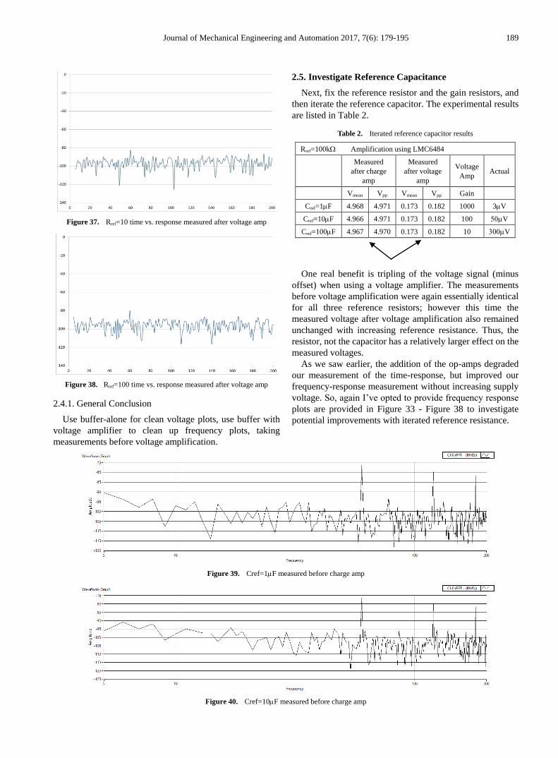
Journal of Mechanical Engineering and Automation 2017, 7(6): 179-195 189
Figure 37. Rref=10 time vs. response measured after voltage amp
Figure 38. Rref=100 time vs. response measured after voltage amp
2.4.1. General Conclusion
Use buffer-alone for clean voltage plots, use buffer with
voltage amplifier to clean up frequency plots, taking
measurements before voltage amplification.
2.5. Investigate Reference Capacitance
Next, fix the reference resistor and the gain resistors, and
then iterate the reference capacitor. The experimental results
are listed in Table 2.
Table 2. Iterated reference capacitor results
Rref=100k Amplification using LMC6484
Measured
after charge
amp
Measured
after voltage
amp
Voltage
Amp Actual
Vmean Vpp Vmean Vpp Gain
Cref=1F 4.968 4.971 0.173 0.182 1000 3V
Cref=10F 4.966 4.971 0.173 0.182 100 V
Cref=100F 4.967 4.970 0.173 0.182 10 V
One real benefit is tripling of the voltage signal (minus
offset) when using a voltage amplifier. The measurements
before voltage amplification were again essentially identical
for all three reference resistors; however this time the
measured voltage after voltage amplification also remained
unchanged with increasing reference resistance. Thus, the
resistor, not the capacitor has a relatively larger effect on the
measured voltages.
As we saw earlier, the addition of the op-amps degraded
our measurement of the time-response, but improved our
frequency-response measurement without increasing supply
voltage. So, again I’ve opted to provide frequency response
plots are provided in Figure 33 - Figure 38 to investigate
potential improvements with iterated reference resistance.
Figure 39. Cref=1F measured before charge amp
Figure 40. Cref=10F measured before charge amp

190 Timothy Sands et al.: Experimental Piezoelectric System Identification
Figure 41. Cref=100F measured before charge amp
Figure 42. Cref=1F measured before voltage amp
Figure 43. Cref=10F measured before voltage amp
Figure 44. Cref=100F measured before voltage amp
On the other hand, measurement after voltage
amplification does not provide much benefit (see Figure 39 -
Figure 44) with respect to frequency response display. All
spikes were not reduced with increasing reference
capacitance as we saw with reference resistance.
2.6. Iterate Rref (w/LM324)
Next, fix the reference capacitor and the gain resistors,
and then iterate the reference resistor, but this time
replacing the op-amp with a LM324 op-amp. The
experimental results are listed in Table 3 with iterations
displayed in Figure 45 – Figure 50.
Table 3. Iterated reference resistor results
Cref=1 F Amplification using LMC6484
Measured
after charge
amp
Measured
after voltage
amp
Voltage
Amp Actual
Vmean Vpp Vmean Vpp Gain
Rref=1k 5.067 5.070 1.368 1.473 1000 3V
Rref=10k 5.068 5.071 1.295 1.412 1000 3V
Rref=100k 5.068 5.070 1.511 1.587 1000 V
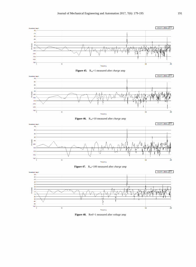
Journal of Mechanical Engineering and Automation 2017, 7(6): 179-195 191
Figure 45. Rref=1 measured after charge amp
Figure 46. Rref=10 measured after charge amp
Figure 47. Rref=100 measured after charge amp
Figure 48. Rref=1 measured after voltage amp

192 Timothy Sands et al.: Experimental Piezoelectric System Identification
Figure 49. Rref=10 measured after voltage amp
Figure 50. Rref=100 measured after voltage amp
2.7. Iterate Cref (w/LM324)
Finally, fix the reference resistor and the gain resistors,
and then iterate the reference capacitor. The experimental
results are listed in Table 4 and the results are displayed in
Figures 51 – Figure 56.
Table 4. Iterated reference resistor results
Rref=100k Amplification using LMC6484
Measured
after charge
amp
Measured
after voltage
amp
Voltage
Amp Actual
Vmean Vpp Vmean Vpp Gain
Cref=1F 5.068 5.070 1.512 1.597 1000 V
Cref=10F 5.068 5.070 1.708 1.762 100 V
Cref=100F 5.068 5.070 1.893 1.931 10 V
Figure 51. Cref=1F measured after charge amp
Figure 52. Cref=10F measured after charge amp

Journal of Mechanical Engineering and Automation 2017, 7(6): 179-195 193
Figure 53. Cref=100F measured after charge amp
Figure 54. Cref=1F measured after voltage amp
Figure 55. Cref=10F measured after voltage amp
Figure 56. Cref=100F measured after voltage amp
3. Results and Discussion
The oscilloscope does a really good job of displaying the
time response (see Figure 6), but the spectral data was more
suspect (noting several different natural frequencies
dependent upon the hardware setup). Especially since system
ID largely comprises identification of the natural frequency,
it is preferred to not modify the measured signal (as is the
case with the oscilloscope). Furthermore, improved spectral
plots result with increased supply voltage (re-examine Figure
19’s spectral plot!) which is not always a good thing.
Therefore we next investigated using buffers. The buffer
provided improved spectral data, but the buffer output did
whatever was necessary to the signal to make the voltages at

194 Timothy Sands et al.: Experimental Piezoelectric System Identification
the inputs equal (again placing us on the path of modifying
the signal). Note the difference between Figure 23 and
Figure 24. Using the op-amps in the buffer configuration
resulted in pretty spectral plots, but there were lots of “ghost”
resonances. Using the op-amps in the two-stage charge
amplifier configuration suppressed the “ghost resonances”.
In all cases, taking measurements at the output of the charge
amplifier was superior to taking measurements at the voltage
amplifier. The two-stage amplification configuration
provided on the order of triple voltage signal (peak minus
offset) amplification. Several of the iterated cases provided
good signal amplification with very legible spectral data
plots. The LMC6484 response was slightly better than the
LM324 response in the buffer configuration, but the opposite
was true in the case of the two-stage amplifier configuration.
This experimental analysis reveals practical techniques for
experimental system identification, in particular of natural
frequencies of piezoelectric elements that are useful to
control very light, highly flexible space appendages that
complicate attitude control, especially instances where
controls-structural integration occur.
4. Summary and Conclusions
Utilizing the methods in this paper, the reader can
accurately estimate system parameters of piezoelectric
elements that can be used to aid the control of highly flexible
space structure. The system estimates can be used to
initialize nonlinear, adaptive attitude control methods based
on the system mathematical models that control both the
rigid body modes and flexible modes of the spacecraft
dynamics. Well-initialized adaptive controllers are able to
achieve high pointing accuracy facilitating operational
missions such as space radar and optical payload support.
ACKNOWLEDGEMENTS
This investigation was guided by Stanford’s Tom Kenny’s
calling to provide working knowledge of modern actuator
technologies. Furthermore, all experimental results were
achieved using Professor Kenny’s laboratory equipment.
REFERENCES
[1] National Instruments, Available online: http://www.ni.com/en-us.html.
[2] National Instruments product detailes website, “myDAQ Student Data Acquisition Device” http://www.ni.com/en-us/shop/select/mydaq-student-data-acquisition-device.
[3] Takuro, I., Fundamentals of Piezoelectricity, Oxford University Press; Oxford, 1990. Also availale online at http://courses.washington.edu/mengr568/ref/piezoelectricity.pdf, accessed 18 Sep 2017.
[4] Gere, James M., Goodno, Barry J., Mechanics of Materials (Eighth ed.), CL Engineering, Canada, pp. 1083–1087. ISBN 978-1-111-57773-5.
[5] Alaneme, K.K., “Design of a Cantilever - Type Rotating Bending Fatigue Testing Machine”, Journal of Minerals & Materials Characterization & Engineering, Vol. 10, No.11, pp.1027-1039, 2011.
[6] Lubliner, J., Plasticity Theory, Dover Publications, (2008). ISBN 0-486-46290-0.
[7] Blake, K., "AN1177 Op Amp Precision Design: DC Errors" (PDF), Microchip, 2008. Available online at: http://ww1.microchip.com/downloads/en/AppNotes/01177a.pdf. Accessed 18 Sep 2017.
[8] Hamilton, S., An Analog Electronics Companion, Cambridge University Press, 2007. ISBN 0-521-68780-2.
[9] National Instruments tutorial, “Using myDAQ with the NI ELVISmx Oscilloscope Soft Front Panel”, http://www.ni.com/tutorial/11502/en/. Accessed 18 Sep 2017.
[10] Lamar University Tutorial, “Mechanical Vibrations”, by Paul Dawkings, available online at: http://tutorial.math.lamar.edu/Classes/DE/Vibrations.aspx, Accessed 18 Sep 2017.
[11] Sands, T., “Space Based Electronic Warfare”, Proceedings of the 43rd AOC International Symposium & Convention, Technical Track 3 Enhancing EW Superiority, 2006.
[12] Sands, T., Kim, J., Agrawal, B., "2H Singularity-Free Momentum Generation with Non-Redundant Single Gimbaled Control Moment Gyroscopes," Proceedings of 45th IEEE Conference on Decision & Control, 2006.
[13] Sands, T. "Fine Pointing of Military Spacecraft," PhD dissertation, Naval Postgraduate School, 2007.
[14] Sands, T., "The Electronic Battle - Requirements and Capabilities" Proceedings of the 44th AOC International Symposium and Convention, Technical Track 3, 2007.
[15] Kim, J., Sands, T., Agrawal, B., "Acquisition, Tracking, and Pointing Technology Development for Bifocal Relay Mirror Spacecraft" SPIE Proceedings Vol. 6569, 656907, 2007.
[16] Sands, T., "Physics-Based Automated Control of Spacecraft" AIAA Space 2009, AIAA #167790, 2009.
[17] Sands, T., "Control Moment Gyroscope Singularity Reduction via Decoupled Control," IEEE SEC Proceedings, 2009.
[18] Sands, T., "Satellite Electronic Attack of Enemy Air Defenses," IEEE SEC Proceedings, 2009.
[19] Sands, Timothy A., "Physics-Based Control Methods," book chapter in Advancements in Spacecraft Systems and Orbit Determination, edited by Rushi Ghadawala, Rijeka: In-Tech Publishers, pp. 29-54, 2012.
[20] Sands, Timothy A., Kim, J. J., Agrawal, B. N., "Nonredundant Single-Gimbaled Control Moment Gyroscopes," Journal of Guidance, Control, and Dynamics, 35(2) 578-587, 2012.

Journal of Mechanical Engineering and Automation 2017, 7(6): 179-195 195
[21] Sands, Timothy A., Kim, J. J., Agrawal, B. N., "Spacecraft Adaptive Control Evaluation", Infotech Aerospace Conference (AIAA 2012-2476), Garden Grove, CA, 2012.
[22] Sands, Timothy A., "Physics-Based Control Methods," book chapter in Advancements in Spacecraft Systems and Orbit Determination, edited by Rushi Ghadawala, Rijeka: In-Tech Publishers, pp. 29-54, 2012.
[23] Nakatani, S., Sands, T., "Simulation of Spacecraft Damage Tolerance and Adaptive Controls", IEEE Aerospace Proceedings, 2014.
[24] Sands, T., "Improved Magnetic Levitation via Online Disturbance Decoupling", Physics Journal, Vol. 1, No. 3, Oct. 19, 2015.
[25] Sands, T., “Experiments in Control of Rotational Mechanics”, International Journal of Automation, Control and Intelligent Systems, (2)1 9-22, Jan. 2016.
[26] Nakatani, S., Sands, T., “Autonomous Damage Recovery in Space”, International Journal of Automation, Control and Intelligent Systems, (2)2 23-36, Jul. 2016.
[27] Sands, T., "Singularity Minimization, Reduction and Penetration", Journal of Numerical Analysis and Applied Mathematics, 1(1) 6-13, 2016.
[28] Heidlauf, P.; Cooper, M. Nonlinear Lyapunov Control Improved by an Extended Least Squares Adaptive Feed Forward Controller and Enhanced Luenberger Observer. In Proceedings of the International Conference and Exhibition on Mechanical & Aerospace Engineering, Las Vegas, NV, USA, 2–4 October 2017.
[29] Sands, T., “Phase Lag Elimination at All Frequencies for Full State Estimation of Spacecraft Attitude”, Physics Journal 3(1) 12, 2017.
[30] Cooper, M.; Heidlauf, P.; Sands, T. Controlling Chaos—Forced van der Pol Equation. Mathematics 2017, 5, 70.
[31] Sands, T., “Space System Identification Algorithms”, Journal of Space Exploration, 2017 (accepted).
[32] Sands, T., “Nonlinear-Adaptive Mathematical System Identification”, Computation, 5(4) 47, 2017.