experimental study and numerical simulation of the flindt ... draft tube... · renewable source of...

1

rapmodfiidp

Tctsc“tco

Jr

1

Downl

Gabriel Dan CiocanResearch Associate

e-mail: [email protected]

Monica Sanda IliescuDoctoral Student


Laboratory for Hydraulic Machines,Ecole Polytechnique Fédérale de Lausanne

(EPFL),Avenue de Cour 33bis,

CH-1007, Lausanne, Switzerland

Thi Cong VuSenior Developement Engineer


Bernd NennemannResearch Assistant


Hydropower Technology,GE Energy,

795 George V,Lachine, Quebec, H8S-4K8, Canada

François AvellanProfessor

Laboratory for Hydraulic Machines,Ecole Polytechnique Fédérale de Lausanne

(EPFL),Avenue de Cour 33bis,

CH-1007, Lausanne, Switzerlande-mail: [email protected]

Experimental Study andNumerical Simulation of theFLINDT Draft Tube RotatingVortexThe dynamics of the rotating vortex taking place in the discharge ring of a Francisturbine for partial flow rate operating conditions and cavitation free conditions is studiedby carrying out both experimental flow survey and numerical simulations. 2D laserDoppler velocimetry, 3D particle image velocimetry, and unsteady wall pressure mea-surements are performs to investigate thoroughly the velocity and pressure fields in thedischarge ring and to give access to the vortex dynamics. Unsteady RANS simulation areperformed and compared to the experimental results. The computing flow domain in-cludes the rotating runner and the elbow draft tube. The mesh size of 500,000 nodes forthe 17 flow passages of the runner and 420,000 nodes for the draft tube is optimized toachieve reasonable CPU time for a good representation of the studied phenomena. Thecomparisons between the detailed experimental flow field and the CFD solution yield toa very good validation of the modeling of the draft tube rotating vortex and, then,validate the presented approach for industrial purpose applications.�DOI: 10.1115/1.2409332�

IntroductionHydropower is a clean form of power generation, which uses a

enewable source of energy: water. Moreover, storage capabilitynd flexible generation makes hydropower the quasi-ideal form ofower generation to meet the variable demand of the electricityarket, therefore it is not surprising that the turbines tend to be

perated over an extended range, far from the optimum flow con-itions. In particular, at part load operating conditions turbinexed-pitch runners show a strong swirl at the runner outlet. As the

ncoming swirling flow is decelerating in the diffuser cone, a hy-rodynamic instability arises under the form of a characteristicrecession flow—see Jacob �1�.

For the usual setting levels of the turbines, defined by thehoma cavitation number �, the static pressure is such that theavitation development makes visible the core of the vortex and,herefore, the precession movement through a typical helicalhape of the cavity in the draft tube cone. The cavitation vortexore of the swirling flow at the runner outlet is the so-calledrope.” The development of cavitation introduces compliance inhe turbine draft tube flow and, consequently, a natural frequencyorresponding in a first approximation to the frequency of the freescillation of the water plug in the draft tube against the compliant

Contributed by the Fluids Engineering Division of ASME for publication in theOURNAL OF FLUIDS ENGINEERING. Manuscript received June 27, 2005; final manuscript
eceived July 10, 2006. Review conducted by Joseph Katz.
46 / Vol. 129, FEBRUARY 2007 Copyright ©

oaded 06 Jul 2009 to 128.178.4.3. Redistribution subject to ASME

vapors volume of the rope. The coupling between this naturalfrequency and the precession frequency leads to the draft tubesurge; see Nishi et al. �2�, which can inhibit the operation of thewhole hydropower plant.

Characterizations of the part load operating conditions havebeen carried out extensively; see Jacob �1�, and the technology forovercoming the draft tube surge through active control has beenestablished. However, any attempt of modeling the hydrodynamicphenomena leading to the development of the rope and its inter-action with all the turbine and hydraulic system components needsfurther investigations.

Recent developments of experimental methods and numericalsimulation techniques permit the detailed analysis of this flow. Itis feasible presently to predict this operating regime, from thepoint of view of the theoretical background, the computationalresources, and the existence of accurate experimental measure-ments to rely on.

The availability of advanced optical instrumentation, such aslaser Doppler velocimetry �LDV� or particle image velocimetry�PIV� systems, gives the opportunity to perform flow surveys inturbomachinery and in particular to investigate the unsteady char-acteristics of the complex flow velocity fields in the case of, forinstance, the rotor-stator interactions, the draft tube, or the spiralcasing.

The progress of the numerical techniques in the prediction ofthe turbine characteristics for the operating ranges in the vicinity
of the beam efficiency point �BEP� insure a good accuracy—see
2007 by ASME Transactions of the ASME

license or copyright; see http://www.asme.org/terms/Terms_Use.cfm

VpRt

ifittltmHSsoatttwl

ttAtcmtjmtsu

dttttbqtiofha

avgd

J

Downl

u et al. �3�. The massively parallel computations developmentermits now the numerical simulation of the whole turbine—seeuprecht et al. �4� or to detail the flow in a specific part of the

urbine.One of the new challenges for the numerical turbine simulation

s to predict the partial or full flow rate operating regimes and therst simulations are promising. Ruprecht et al. �5� are focused on

he influence of different turbulence models on the modeling ofhe draft tube vortex, carried out in a straight cone. Based on theength of the predicted vortex structure, certain turbulence modelsend to have a damping effect and from this point of view, the

ost accurate, is found to be a two-scale model described byanjalic, reduced to a two equations set by a Very Large Eddyimulation �VLES� approach. The validation of the numericalimulation is performed on a Francis turbine draft tube with threeutlet channels. For a relatively coarse mesh—250,000 nodes—nd the computed runner outlet velocity profile as inlet conditions,he vortex frequency is well predicted—93% of the measured vor-ex frequency, but an underestimation of the wall pressure fluc-uation amplitudes is obvious. The given explanation turns to-ards the possible variation of the flow rate during operation at

ow flow rate.Scherer et al. �6� reported the turbine design improvement for

he draft tube operating at partial flow rate conditions by Compu-ational Fluid Dynamics �CFD�. An unsteady one-phase Reynold’sveraged Navier-Stokes �RANS� simulation of the draft tube vor-

ex in a Francis turbine model is used to compare two draft tubeonfigurations. By comparing the calculated performances of twoodel machines over the operating range, the second one is found

o have better draft tube efficiency at low flow rate operation,ustified by the obtained pressure pulsations improvement, the di-

inishing of the strong velocity gradients, and backflow zone inhe cone. The comparison with wall pressure experimental datahows a good agreement for the vortex frequency and a systematicnderestimation of the pressure fluctuation amplitudes.

Miyagawa et al. �7� performed an unsteady simulation of theraft tube vortex for a Francis pump turbine, consecutively forwo different runners. The purpose was to analyze the influence ofhe velocity profile at the runner outlet on the flow instability inhe draft tube. Two runner designs are tested for the same draftube geometry—using a mesh of 620,000 nodes. The same vortexehavior changes are observed in CFD and experimentally byualitative comparisons with the rope visualizations. The authorsested a one phase and a two-phase model as well, and found thatt influences mainly the fluctuation amplitude and has no influencen the vortex frequency, but no further details are given. The voidraction in the vortex core is found to be similar compared toigh-speed camera visualizations, but quantitative comparisonsre not available.

In the last two papers, the inlet boundary conditions are takens the result of the steady calculation of the runner and/or guideanes—stay vanes. It provides, thus, the uniform axial and tan-ential velocity profile, circumferentially averaged. As outlet con-

Table 1 Bibliographical result of the CF

Comparison betweenexperimental andnumerical data Ruprecht et al.a ScheCFD fr/Experimental fr

0.93res

CFD pressure pulsationamplitude/experimentalpressure pulsation amplitude

0.7–1.3

aSee Ref. �5�.bSee Ref. �6�.cSee Ref. �7�.dSee Ref. �8�.

ition, a constant pressure value is considered.

ournal of Fluids Engineering


Sick et al. �8� performed a numerical simulation of a pumpturbine with a Reynolds stress turbulence model, already validatedfor near BEP operating conditions. Unlike other studies, the run-ner and the outlet domain were included in the computationaldomain with 1.5 million of cells for minimizing the steady inletvelocity profile effect and the uniform outlet pressure boundarycondition effect. The comparison with experimental data shows anoverestimation of the vortex frequency and a quite good agree-ment for the pressure fluctuations amplitude. The analysis of theforces and bending moments on the runner shaft due to the vortexgives the same characteristics like the pressure pulsations: a goodagreement for the amplitude and an overestimation of the fre-quency.

These papers get to a fairly good agreement with the globalcharacteristics of the flow—see Table 1, but a validation impliesthe validations of the partial flow rate vortex phenomenology andalso comparisons of the detailed flow field.

In the frame of the FLINDT—flow investigations in drafttubes—project, Eureka No. 1625, the operation in low flow rateconditions of a Francis turbine is investigated, both experimen-tally and numerically.

The present paper describes:

— FLINDT phase 2 experimental LDV, PIV, and wall pres-sure measurements for the rotating vortex study in non-cavitating regime in the cone of the draft tube. In thispaper only the local measurements in the cone region willbe presented;

— CFD methodology for the unsteady simulation of the ro-tating vortex;

— comparison of the numerical solution with experimentaldata.

2 Experimental Approach for the Draft Tube RotatingVortex Measurement Scale Model of Francis Turbine

The investigated case corresponds to the scale model of theFrancis turbines of high specific speed, �=0.56 �nq=92� of a hy-dropower plant built in 1926, owned by ALCAN. The 4.1 m di-ameter runners of the machines were upgraded in the late 1980s.The original draft tube geometry is of Moody type. For the pur-pose of the FLINDT research project, an especially designed el-bow draft tube with one pier replaces the original Moody drafttube. The scale model—D1̄e=0.4 m—is installed on the third testrig of the EPFL Laboratory for Hydraulic Machines and the testsare carried out according to the IEC 60193 standards �9�.

The energy-flow coefficients and efficiency characteristics ofthe scale model are represented on the hill chart in Fig. 1. Accord-ing to the objective of the study, an operating point is selected atpartial flow rate condition. The point of interest is selected for aspecific energy coefficient of �=1.18 and a flow rate coefficient of�=0.26, which corresponds to about 70% QBEP and a Re number

6

experimental global values comparison

et al.b Miyagawa et al.c Sick et al.d This paperw

tion�Not

available1.12 1.13

.4 Notavailable

0.83 1

D/

rer1 �loolu1–1

of 6.3�10 .

FEBRUARY 2007, Vol. 129 / 147


Ls

itttc

N�esregp

1

Downl

Three different measurement methods are used: 3D PIV, 2DDV, and unsteady wall pressure. The investigated zones are pre-ented in Fig. 2.

2.1 Particle Image Velocimetry Instrumentation. The 3Dnstantaneous velocity field in the cone is investigated with a Dan-ec M.T. 3D PIV system, which consists of a double-pulsed laser,wo double-frame cameras, and a processor unit for the acquisi-ion synchronization and the vectors detection by crossorrelation.

The illuminating system is composed of two laser units witheodynium-doped Yttrium Aluminium Garnet crystals

Nd:YAG�, each delivering a short impulse of 10 ns and 60 mJnergy at 8 Hz frequency. Thus the time interval between twouccessive impulses can easily be adjusted within 1 �s–100 msange, depending on the local flow characteristics or the phenom-non, which is to be captured. The output laser beam of 532 nm isuided through an optical arm, for accessibility, to a beam ex-ander and transformed into a sheet of 4 mm width and 25 deg

Fig. 1 Scale model hill char

Fig. 2 Measurement zones in th

48 / Vol. 129, FEBRUARY 2007


divergence.Two Hi-Sense cameras with a resolution of 1280�1024 pixels

are used for 200�150 mm2 investigation area. The cameras areplaced in a stereoscopic configuration, focused on the laser-sheet,synchronized with the two pulses. They capture the position ofseeding particles of �10 �m diameter by detecting their scatteredlight. In order to avoid possible reflections in the laser wavelengthon the cameras, due to the optical interfaces or to residual bubblesin the flow, fluorescent particles of 580 nm emission wavelengthare used, along with corresponding cutoff filters on the cameras.

For the optical access, the cone is manufactured in Polymethylmethacrylate �PPMA� with a refractive index of 1.4, equippedwith a narrow window for the laser’s access and two large sym-metric windows for the cameras access, having a flat externalsurface for minimizing the optical distortions.

The corresponding two-dimensional vector maps, obtainedfrom each camera by a fast Fourier transform-based algorithm, arecombined in order to have the out-of-plane component, character-

nd part load operating point
t a
e cone of the FLINDT turbine

Transactions of the ASME


i

smetifiFa0e3

lma

ulpsbTvt�

w

J

Downl

zing the displacement in the laser-sheet width.The correlation between the local image coordinates and real

pace coordinates is realized through a third order optical transferatrix, which includes the correction of distortions due to differ-

nt refractive indices in the optical path and to the oblique posi-ion of the cameras. The calibration relation is obtained acquiringmages of a plane target with equally spaced markers, moved inve transversal positions in order to have volume information, seeig. 3. The target displacement in the measurement zone, withccuracy within the narrow limits of 0.01 mm in translation and.1 deg in rotation, insured a good calibration quality; see Iliescut al. �10�. The overall uncertainty of the PIV 3D velocity fields is% of the mean velocity value.

2.2 Laser Doppler Velocitry Instrumentation. The 2D ve-ocity profile survey is performed by the LDV measurement

ethod—see Fig. 2, on two complete diameters, at the cone inletnd outlet.

The LDV system is a Dantec M.T. two components system,sing backscattered light and transmission by optical fiber, with aaser of 5 W argon-ion source. An optical window with plane andarallel faces is used as interface. The geometrical reference po-ition of the measurements is obtained by positioning the lasereams on the windows faces with accuracy better than 0.05 mm.wo components are measured: the tangential component of theelocity Cu and the axial one Cz, see Fig. 2. The uncertainties ofhe laser measurements are estimated to 2%—see Ciocan et al.11�.

2.3 Unsteady Wall Pressure Instrumentation. The unsteadyall pressure measurements—100 simultaneous acquisitions—

Fig. 3 Calibration setup for 3D PIV measurements

Fig. 4 Phase average calculation of



permit to discriminate the rotating pressure field due to the vortexrotation and the synchronous pressure field at the samefrequency—see Arpe. �12� In order to capture the phenomena ofinterest in low flow rate turbine operating conditions, all pressuresignals are acquired simultaneously with a HP-VXI acquisitionsystem using a sampling frequency of 16�n, 80�n and 214

samples. The spectral analysis does not show differences betweenthe three sampling frequencies, thus for the analysis it was chosenthe 16�n acquisition rate. This setup allows recording 430 vortexpassages, providing an acceptable number of segments for theaveraging process and insuring an uncertainty of 3%.

The pressure field evolution, depending on the Thoma number,is obtained in the whole draft tube. Only eight pressure sensors inthe cone will be presented in this paper, corresponding to thepositions described in Fig. 2.

2.4 Data Post Processing. For periodic flows, the signal isreconstructed by synchronizing the acquisition with a referencesignal at several time shifts �—Fig. 4. The reference signal comesfrom a pressure sensor and the pressure drop corresponding to thevortex passage is used for triggering all acquisitions.

Thus the periodic signal can be decomposed according to

Ci�t� = C̄ + C̃�� + C��t� �1�

The phase-locked component C̃+ C̄ is obtained by averaging theinstantaneous values at the same � value; see Eq. �3�

C̄ = �Ci� = limN→�

1

N�i=1

N

Ci�t� �2�

C̃�� = limN�→�

1

N��i=1

N

�Ci�� − C̄� �3�

with

C̃¯

= 0�4�

�C�� = limN→�

�Ci�t� − C̄ − C̃� = 0

Fifteen phase values, equidistant in a vortex passage interval, Tr,are selected to complete the phase average. Thus the vortex syn-chronous flow is reconstituted.

The LDV acquisition is triggered with the wall pressure signalbreakdown given by the vortex passage. The LDV data signal isnot continuous, thus an additional reference signal is taken froman optical encoder mounted to the runner shaft. The resolution ofthe optical encoder is 0.04 deg of runner rotation. In this way we

the LDV and PIV velocity signal

FEBRUARY 2007, Vol. 129 / 149


htswm

q1

C̄v

s

ht

1

Downl

ave the relation between the runner spatial position and the vor-ex period. Thus each LDV acquisition is reported to the corre-ponding vortex period via the runner position—see Fig. 4. In thisay the fluctuation of the vortex period is obtained at 3% of itsean value.Subsequent to a mean convergence study, the number of ac-

uired velocity values for each phase, � value, has been between000 and 3000 instantaneous values, thus the mean velocity value

represents the statistic over 30,000 instantaneous velocityalues.

For the PIV measurements, subsequent to a mean convergencetudy, the number of acquired vector maps for each phase, � value,

as been set to 1200, thus the mean velocity value C̄ representshe statistic over 18,000 instantaneous velocity fields. The PIV

Fig. 5 LDV-PIV phas

Fig. 6 Waterfall diagram and

50 / Vol. 129, FEBRUARY 2007


acquisition is performed at constant � value reported to the vortextrigger signal—see Fig. 4. The influence of the vortex periodvariation for this kind of phase average calculation is checked andfits within the same uncertainty range like the measurementmethod 3%—see Fig. 5.

The direct comparison between the mean velocity values, seeFig. 12, or phase average velocity values, see Fig. 5, obtained byLDV and PIV measurements in the upper part of the cone, showsan excellent agreement as well.

Concerning the phase average calculations for the unsteadypressure acquisition—at constant acquisition rate—and for the nu-merical results, they are performed by averaging the instantaneousvalues for each � interval.

2.5 Description of the Study Case. The experimental inves-

verage comparison

rresponding cavitation ropes

e a

co



tvmaav

fccc

3

Rbaknbcutcrppt

spfisosaatbaniactm

J

Downl

igation is carried out for a range of Thoma cavitation numbersarying from �=1.18, cavitation free conditions, to �=0.38,aximum rope volume. For a given operating point, same head

nd flow rate, the vortex frequency, pressure pulsation amplitudend volume of vapor in the vortex core are dependent of the �alue as shown on the waterfall diagram in Fig. 6.

Since, for the moment, the numerical simulation is performedor single-phase flow condition, the study case is limited to theavitation free condition, �=1.18. The present operating pointorresponds to a flow coefficient �=0.26 and a specific energyoefficient �=1.18.

Numerical Simulation of Unsteady Flow Behavior

3.1 CFD Methodology for the Unsteady Simulation of theotating Vortex. Nowadays it became common to predict flowehavior and energy loss in hydraulic turbine components by CFDpplication, using a Navier–Stokes flow solver closed with the-epsilon turbulence model. When individual hydraulic compo-ents are optimized, then steady state stage flow analysis for com-ined hydraulic components is performed to establish the effi-iency of the entire turbine—see Vu et al. �3�. For investigation ofnsteady flow behavior in hydraulic turbine components, such ashe rotating rope phenomena in draft tubes at partial flow rateondition or the interaction of flow between wicket gates andunner blades, unsteady flow computation is required. For theresent application, ANSYS-CFX 5.6 version is used for the com-utation. Also the standard k-epsilon turbulence model is used forhe flow simulation.

3.2 Choice of Computational Flow Domain. For the un-teady flow simulation of the rotating vortex rope, there are threeossible configurations for the computational flow domain. Therst configuration considers only the draft tube geometry. Theecond configuration includes runner and draft tube, and the thirdne includes wicket gates, runner, and draft tube geometries. Theecond configuration is selected here for the unsteady simulations the best compromise between solution accuracy requirementsnd computer resources. The transient runner/draft tube simula-ion allows us to predict the true unsteady interaction of the flowetween the upstream runner and the elbow draft tube. In thispproach, the unsteady relative motion between the two compo-ents on each side of the general grid interface �GGI� connections simulated. The interface position is updated for every time step,s the relative position of the grids on each side of the interfacehanges. Figure 7 represents the computational flow domain forhe unsteady flow simulation and the multi block structured

Fig. 7 Computation

eshes generated for the runner and the draft tube. An O type



420,000 node mesh is used for the draft tube and an H mesh typewith 500,000 nodes is generated for the 17 flow passages of therunner. Due to a foreseen requirement of very large Central Pro-cessing Unit �CPU� time for the computation, we prefer to keep arelatively coarse mesh size for the application.

3.3 Computational Procedure for Unsteady FlowSimulation. Two preliminary steady state calculations were per-formed, the first one for the spiral casing and the distributor, andthe second one for the stay vane, guide vane, and runner assembly.The results of the first calculation were used as inlet conditions forthe second calculation. In turn, the inlet conditions for the un-steady calculation—including turbulent kinetic energy and dissi-pation rate profiles—were extracted form the second steady statecalculation. The average turbulence intensity at inlet to the un-steady calculation domain is about 3.5% while the average rela-tive viscosity is 110. In this way, for the unsteady computationaldomain—runner and draft tube—the flow rate, flow direction, andthe turbulence intensity obtained in the second steady preliminarycalculation are specified as the inlet boundary conditions. Theoutlet condition is the zero gradient condition in the outflow di-rection is applied for all variables.

Since we are interested in simulating a periodic-in-time quasi-steady state, it is recommended to first obtain a steady state solu-

Fig. 8 Evolution of pressure monitoring in transient

w domain and mesh

computation

flo

FEBRUARY 2007, Vol. 129 / 151


tsTbmieo

wa

1

Downl

ion using the stage flow calculation and then using this steadytate solution to start the unsteady runner/draft tube simulation.he transient solution should converge to the desired periodicehaviour after several runner revolutions. For hydraulic turbineachines, using time step of about 1 time step /deg of revolution

s satisfactory. The rms convergence criterion of the residual forach time step is specified to 10−4. Figure 8 shows the evolutionf pressure monitoring in the draft tube cone during the transient

Fig. 9 Comparison of CFD an

Fig. 10 Period adjustment and phase shift on the n

Fig. 11 Phase average

52 / Vol. 129, FEBRUARY 2007


computation. It takes about 1000 time steps to start the fluctuationfrom a steady state solution and another 3000 time steps to reachthe periodic unsteady state. Then starting from that point, we ob-tain a periodic signal at the cone region as shown in Fig. 8. Thenumerical solution is considered to be well converged after 11,500time steps or after 24 runner revolutions. The computation is car-ried out on a Beowulf Linux cluster. It takes about 25 CPU daytime in parallel computing with 4 CPUs.

xperimental frequency spectra

erical data to compare with the experimental ones

ll pressure comparison

d e

um



dstdFtvps

4m

rtadtq0g

fnaThmd

J

Downl

Unsteady flow computations generate tremendous amounts ofata if one wants to write a transient solution for every single timetep. It is preferable that monitoring points are specified at loca-ions of interest during the preprocessing stage and only interme-iary transient solutions are written at a certain interval time step.or the present application, during the last 2500 time steps, moni-

or points are specified for all locations at which pressure andelocity components �PIV� are measured for a total of about 1200oints. Also, transient solutions are written for every ten timeteps.

Comparison of the Numerical Solution With Experi-ental Data

4.1 Validation With Global Quantities. For the partial flowate operating points, the determining parameters for the interac-ion between the machine and the circuit are the vortex frequencynd the associated pressure amplitude pulsations. The waterfalliagram, as shown in Fig. 6, gives a three-dimensional represen-ation of the pressure fluctuation amplitude spectra in the fre-uency domain for each � value. This frequency varies between.3 and 0.36 of the runner revolution frequency for the � investi-ation range.

4.1.1 Vortex Frequency. For �=1.18, the vortex frequencyrom the experimental data is 0.30 of the runner revolution. Theumerical vortex frequency obtained by frequency spectrumnalysis is 0.34 of the runner revolution frequency—see Fig. 9.hus the numerical simulation vortex frequency is about 13%igher than the measured vortex frequency but it falls within theeasured variation range for the � values in these operating con-

Fig. 12 Mean velocity pro

itions.



4.1.2 Pressure Fluctuation Amplitude. For comparing thephase average pressure fluctuation resulting from the numericalcalculation with the experimental results, the phase reference ofthe numerical simulation is adjusted in order to match the phase ofthe experimental signal. Therefore, the phase reference is chosenfor an experimental sensor: all the others begin synchronized withthis one. The numerical phase—without any physicalsignificance—is adjusted on the position of the experimental sen-sor and all numerical phase averages are corrected with this phaseshift �difference� �—see Fig. 10.

To be coherent for the period representations, the experimentalperiod was chosen like reference and the numerical period isstretched to a dimensionless vortex period as follows:

� = �Numerical − �

kr =TrNumerical

TrExperimental�5�

� = �Experimental · kT

Figure 2 shows monitor points for static pressure at differentsection planes. Figure 11 shows the comparison of the numericalstatic pressure fluctuation with the experimental data for one pe-riod of the vortex. Both signals are normalized with their ownvortex frequency. The correlation between the numerical simula-tion and the experimental data is excellent. The pressure fluctua-tion amplitude is well predicted not only at the runner outlet, butits evolution in the cone is in good agreement with the experimen-

s comparison in the cone
file
tal data for all sensors angular positions, as well—see Fig. 2. The

FEBRUARY 2007, Vol. 129 / 153


1

Downl

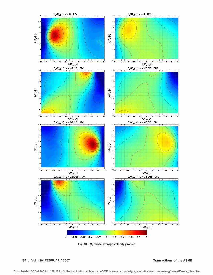
Fig. 13 C phase average velocity profiles
z
54 / Vol. 129, FEBRUARY 2007 Transactions of the ASME

oaded 06 Jul 2009 to 128.178.4.3. Redistribution subject to ASME license or copyright; see http://www.asme.org/terms/Terms_Use.cfm

J

Downl

Fig. 14 C - C phase average velocity profiles comparison in the cone
r z
ournal of Fluids Engineering FEBRUARY 2007, Vol. 129 / 155

oaded 06 Jul 2009 to 128.178.4.3. Redistribution subject to ASME license or copyright; see http://www.asme.org/terms/Terms_Use.cfm

drs

tam

tzltsPavs

vTsstTts

Lsps

uat

prpptcpl

Et

brvip

ctptvTnav

1

Downl

ifference between the experimental results and numerical oneseported to the mean pressure level is less than 2.5%, so in theame range as the measurement accuracy.

4.2 Validation with Local Flow Structure. For improvinghe turbines design it is necessary to predict the real flow structurend associated phenomenology throughout the entire analyzed do-ain.

4.2.1 Mean Velocity Profiles. The mean flow velocity showshe decelerated swirling flow that develops in a central stagnationone—see Fig. 12. The vortex encloses this zone of average ve-ocity near zero. The flow rate distribution is therefore restricted tohe circular zone between the cone walls and the vortex conicalupporting surface. The LDV measurements that complete theIV measurements in the inlet and outlet cone cross sections showhigher velocity near the cone wall, for the axial and tangential

elocity. The angle at which the stagnation region develops down-tream is higher than the angle of the turbine cone.

For assessing the flow structure prediction, the numerical meanelocity field is compared with the LDV and PIV measurements.he comparison of the flow structure in the cone of the turbinehows a generally good agreement of the velocity mean values—ee Fig. 12. A small difference is observed at the runner outlet inhe strong velocity gradients zone—between R /Rout=0.2 to 0.35.he numerical results are smoother, and for this reason the zone of

he mean near zero velocities, in the centre of the cone, is not theame.

4.2.2 Phase Average Velocity Field. For the comparison ofDV and PIV velocity measurements with the CFD results, theame procedure like for the pressure is considered: the numericaleriod is shifted onto the experimental one and the same phasehift � is applied for all numerical velocity signals.

The central stagnation zone, observed in the time averaged val-es, represents the zone closed by the vortex passage in phaseverage values. This region is a series of backflows, triggered byhe vortex passage—see Fig. 13.

The phase average vector field representation shows the vortexosition in the measurement section—see Fig. 14. The phase cor-espondence obtained by the pressure fitting is the same as for thehase velocity profiles. Qualitatively the vortex center position islaced on the same cone height. A small difference is observed inhe radial position, in the numerical simulation, it is closer to theone wall. This difference is in accordance with the mean velocityrofile. The phase average flow structure of the numerical simu-ation is very similar to the experimental measurements one.

4.2.3 Vorticity Field. The calculation of the vorticity—seeq. �6�, for each phase averaged velocity field, permits to quantify

he vortex evolution in the measurement zone.

� = �� C� �6�As represented in Fig. 15, the vortex position is well predicted

y the numerical calculations, with a difference of 5% of theadius between the predicted position and the measured one. Theorticity is smaller in numerical calculations with about 18%, butts position closer to the cone walls explains the fact that the sameressure fluctuation amplitude values are obtained at the wall.

4.2.4 Vortex Center. The vortex center position is estimatedonsidering the vortex center as the maximum vorticity point inhe cone section which corresponds to the stagnation point in thehase average flow field—see Fig. 16. The vortex position trace inhe section is similar with the rope position visualization by theapors zone in the section for the low sigma numbers—see Fig. 6.he comparison of the vortex center between experimental andumerical data is representative for the vortex phenomenologynd the difference between the center position, as well as the
orticity intensity, could by explained by the relatively coarse
56 / Vol. 129, FEBRUARY 2007


mesh compared to the vortex size—see Fig. 17. The mesh size ischosen as the best compromise between the result quality and therequired computational time.

5 Concluding RemarksThis paper has presented a CFD methodology to study the un-

steady rotating vortex in the FLINDT draft tube and associatedexperimental study of the flow phenomena.

A large experimental database is built in the frame of theFLINDT project for partial flow rate operating regime. 3D PIV,2D LDV, unsteady wall pressure, and unsteady wall friction mea-surements are available for analysis, with certified accuracy.

The transient flow simulation is for single phase using a stan-dard k-epsilon turbulence model. Although a relatively coarsemesh is used for the computational, an excellent agreement be-tween numerical results and experimental data is obtained. Theaccuracy of the prediction for the vortex global quantities, pres-sure pulsation amplitude �3% error�, and vortex frequency �13%error� is very good. For the first time the simulated vortex struc-ture of the rotating vortex is assessed and compared with experi-mental measurements. The quantitative analyses in terms of meanvelocity field, phase average velocity field, vorticity, and vortexcenter position also show a good agreement and validate the phe-nomenology of the vortex rope in numerical simulations. We can

Fig. 15 Vorticity field in the cone

Fig. 16 Vortex center evolution in the cone



uCutt

wtp

A

pd�atltaadEf

N

J

Downl

se with confidence this approach for design purpose application.ompared with a classical steady simulation, the unsteady CFDsed for partial flow rate simulation provides important informa-ion for the machine design: the wall pressure unsteady fluctua-ions level and velocity field structure.

In the future the extension of this approach to two phase flowsill permit to take into account another important parameter for

he partial flow rate phenomenology: the cavitation and its com-liance.

cknowledgmentThe authors take this opportunity to thank our FLINDT

roject—Eureka No. 1625—partners: Alstom Hydro, Electricitée France, VA Tech Escher Wyss Hydro, Voith Hydro, PSELFunds for Projects and Studies of the Swiss Electric Utilities�,nd the CTI �Commission for Technology and Innovation�, forheir financial support and the staff of the Laboratory for Hydrau-ic Machines for the technical support. We would also like tohank Jorge Arpe for the unsteady wall pressure measurementsnd Olivier Braun for the numerical results postprocessing. Theutomatic mesh generators used for runner and draft tube wereeveloped under GMATH, a collaborative project between GEnergy and Ecole Polytechnique de Montreal, coordinated by Pro-

essor Francois Guibault.

omenclatureE � specific energy �J /kg�Q � flow rate �m3/s�

QBEP � flow rate at the best efficiency operating condi-tion �m3/s�

� � cavitation numberD1̄e � runner diameter �m�

Ci � instantaneous velocity �m/s�C̃ � periodic fluctuating component �m/s�C̄ � time-averaged velocity value �m/s�

C� � random turbulent fluctuation �m/s�Cu � tangential component �m/s�Cz � axial component �m/s�Cr � radial component �m/s�C

Fig. 17 Mesh size in t

� absolute velocity �m/s�



Cref � mean flow reference velocity Cref=Q /A�m/s�� specific energy coefficient� � flow rate coefficient

Cp � pressure coefficient Cp= �p− p̄� /1 /2�cm1̄

2

� rotational velocity �rad/s��Z � cone height �m�

Z � cone’s current depth �m�R � local cone radius �m�

Rout � cone outlet radius �m�fr � vortex rotation frequency �Hz�n � runner rotation frequency �Hz�� phase delay �s�� angular position of the vortex �=2��fr �rad�

Tn � runner rotation period �s�Tr � vortex rotation period �s�

BEP � best efficiency operating pointRe � re number Re=UD /�=�ND2 /60�

References�1� Jacob, T., 1993, “Evaluation sur Modèle Réduit et Prédiction de la Stabilité de

Fonctionnement des Turbines Francis,” EPFL Thesis No. 1146, Lausanne,Switzerland.

�2� Nishi, M., Matsunaga, S., Kubota, T., and Senoo, Y., 1984, “Surging Charac-teristics of Conical and Elbow-Type Draft Tubes,” in Proceedings of the 12thIAHR Symposium, pp. 272–283.

�3� Vu, T. C., and Retieb, S., 2002, “Accuracy Assessment of Current CFD Toolsto Predict Hydraulic Turbine Efficiency Hill Chart,” Proceedings of the 21stIAHR Symposium on Hydraulic Machinery and Systems, Lausanne, Switzer-land, pp. 193–198.

�4� Ruprecht, A., Maihöfer, M., Heitele, M., and Helmrich, T., 2002, “MassivelyParallel Computation of the Flow in Hydo Turbines,” Proceedings of the 21stIAHR Symposium on Hydraulic Machinery and Systems, Lausanne, Switzer-land, pp. 199–206.

�5� Ruprecht, A., Helmrich, T., Aschenbrenner, T., and Scherer, T., 2002, “Simu-lation of Vortex Rope in a Turbine Draft Tube,” Proceedings of the 21st IAHRSymposium on Hydraulic Machinery and Systems, Lausanne, Switzerland, pp.259–266.

�6� Scherer, T., Faigle, P., and Aschenbrenner, T., 2002, “Experimental Analysisand Numerical Calculation of the Rotating Vortex Rope in a Draft Tube Op-erating at Part Load,” Proceedings of the 21st IAHR Symposium on HydraulicMachinery and Systems, Lausanne, Switzerland, pp. 267–276.

�7� Miyagawa, K., Tsuji, K., Yahara, J., and Nombra, Y., 2002, “Flow Instabilityin an Elbow Draft Tube for a Francis Pump-Turbine,” Proceedings of the 21stIAHR Symposium on Hydraulic Machinery and Systems, Lausanne, Switzer-land, pp. 277–286.

vortex center position
he
�8� Sick, M., Dorfler, P., Michler, W., Salllaberger, M., and Lohmberg, A., 2004,

FEBRUARY 2007, Vol. 129 / 157


1

Downl

“Investigation of the Draft Tube Vortex in a Pump-Turbine,” Proceedings ofthe 22nd IAHR Symposium on Hydraulic Machinery and Systems, Stockholm,Sweden.

�9� IEC 60193 Standard, 1999, “Hydraulic Turbines, Storage Pumps and Pump-Turbines-Model Acceptance Tests,” International Electrotechnical Commis-sion, Genève, Switzerland.

�10� Iliescu, M. S., Ciocan, G. D., and Avellan, F., 2002, “3D PIV and LDV Mea-surements at the Outlet of a Francis Turbine Draft Tube,” Joint U.S. ASME—European Fluids Engineering Summer Conference, Montreal, Quebec, Canada,

58 / Vol. 129, FEBRUARY 2007


Paper No. FEDSM2002-31332.�11� Ciocan, G. D., Avellan, F., and Kueny, J. L., 2000, “Optical Measurement

Techniques for Experimental Analysis of Hydraulic Turbines Rotor-Stator In-teraction,” ASME Fluid Engineering Conference, Boston, Paper No.FEDSM2000-11056.

�12� Arpe, J. A., and Avellan, F., 2002, “Pressure Wall Measurements in the WholeDraft Tube: Steady and Unsteady Analysis,” Proceedings of the 21st IAHRSymposium on Hydraulic Machinery and Systems, Lausanne, Switzerland.



experimental study and numerical simulation of the flindt ... draft tube... · renewable source of...

Documents